investigation of the biophysical basis for cell organelle ... · pdf fileinvestigation of the...
TRANSCRIPT

Investigation of thebiophysical basis for cell
organelle morphology
Diplomarbeit
zur Erlangung des wissenschaftlichen Grades
Diplom - Physiker
vorgelegt von
Jurgen Mayer
geboren am 14.03.1977in Biberach
Max-Planck-Institut fur Molekulare Zellbiologie und GenetikFachrichtung Physik
Fakultat fur Mathematik und NaturwissenschaftenTechnische Universitat Dresden
2008


1. Gutachter: Prof. Jonathon Howard
2. Gutachter: Prof. Petra Schwille
Datum des Einreichens der Arbeit: 12. Februar 2008

Abstract
It is known that fission yeast Schizosaccharomyces pombe maintains its nuclearenvelope during mitosis and it undergoes an interesting shape change during celldivision - from a spherical via an ellipsoidal and a peanut-like to a dumb-bellshape. However, the biomechanical system behind this amazing transformationis still not understood. What we know is, that the shape must change due toforces acting on the membrane surrounding the nucleus and the microtubulebased mitotic spindle is thought to play a key role. To estimate the locationsand directions of the forces, the shape of the nucleus was recorded by confocallight microscopy. But such data is often inhomogeneously labeled with gapsin the boundary, making classical segmentation impractical. In order to accu-rately determine the shape we developed a global parametric shape descriptionmethod, based on a Fourier coordinate expansion. The method implicitly as-sumes a closed and smooth surface. We will calculate the geometrical propertiesof the 2-dimensional shape and extend it to 3-dimensional properties, assumingrotational symmetry. Using a mechanical model for the lipid bilayer and the socalled Helfrich-Canham free energy we want to calculate the minimum energyshape while respecting system-specific constraints to the surface and the en-closed volume. Comparing it with the observed shape leads to the forces. Thisprovides the needed research tools to study forces based on images.
Zusammenfassung
Es ist wohlbekannt, dass die Spalthefe Schizosaccharomyces pombe wahrend derMitose ihren Zellkern aufrechterhalt, welcher dafur einen interessanten Gestalt-wandel durchlauft - von einem anfanglich spharischen uber einen ellipsoiden underdnussahnlichen bis hin zu einem hantelformigen Gebilde. Der zugrundeliegen-de biomechanische Mechanismus, der hinter dieser faszinierenden Verwandlungsteckt, ist bis heute unbekannt. Es mussen Krafte auf die Zellkernmembranwirken und man geht davon aus, dass die aus Mikrotubuli bestehende polareSpindelfaser hierbei eine entscheidende Rolle spielt. Um Ort und Richtungder wirkenden Krafte zu bestimmen, wird der Zellkern mittels konfokaler Licht-mikroskopie erfasst. Die hierbei oft ungleichmassige Markierung kann zu Luckenin der Umrandung fuhren, wodurch klassische Segmentierungstechniken nurschwer nutzbar sind. Um dennoch die Gestalt genau zu bestimmen entwickeltenwir eine parametrische Beschreibungsmethode, die auf Fourierreihenentwicklungbasiert. Diese Methode geht implizit von einer geschlossenen, glatten Oberflacheaus. Es werden sowohl die geometrischen Eigenschaften der zweidimension-alen Kontur berechnet, als auch diejenigen, die bei der Rotation dieser Konturentstehenden Dreidimensionalen. Mit Hilfe des Lipid-Doppelschichten-Modells,bei dem keine Scherfestigkeit angenommen wird, wollen wir die minimalener-getische Gestalt unter Vorgabe von Randbedingungen wie der Oberflache unddem eingeschlossenen Volumen berechnen. Die Krafte konnen dann aus demVergleich mit der tatsachlich vorkommenden Form gewonnen werden. Damitkonnen wir Krafte untersuchen, die auf Bildinformationen beruhen.


Contents
1 Introduction 11.1 General Introduction . . . . . . . . . . . . . . . . . . . . . . . . . 11.2 Biological background . . . . . . . . . . . . . . . . . . . . . . . . 2
1.2.1 The nucleus . . . . . . . . . . . . . . . . . . . . . . . . . . 31.2.2 Labeling with Cut11-GFP . . . . . . . . . . . . . . . . . . 5
1.3 Confocal fluorescence microscopy . . . . . . . . . . . . . . . . . . 81.3.1 Principles of laser scanning confocal microscopy . . . . . . 81.3.2 The Point-Spread-Function . . . . . . . . . . . . . . . . . 81.3.3 Microscope setup . . . . . . . . . . . . . . . . . . . . . . . 101.3.4 Sample preparation . . . . . . . . . . . . . . . . . . . . . 11
2 Methods 132.1 Fourier series and Fourier expansion . . . . . . . . . . . . . . . . 13
2.1.1 Introduction to Fourier series . . . . . . . . . . . . . . . . 132.1.2 Fourier series representation . . . . . . . . . . . . . . . . . 162.1.3 Fourier coordinate expansion . . . . . . . . . . . . . . . . 172.1.4 Meaning of the coefficients . . . . . . . . . . . . . . . . . 21
2.2 The 2-d-contour-explorer . . . . . . . . . . . . . . . . . . . . . . . 232.3 Shape analysis . . . . . . . . . . . . . . . . . . . . . . . . . . . . 25
2.3.1 Decreasing amplitudes and truncation of the series . . . . 252.3.2 Calculating the 2-dimensional properties . . . . . . . . . . 262.3.3 Program testing . . . . . . . . . . . . . . . . . . . . . . . 302.3.4 The Elephant . . . . . . . . . . . . . . . . . . . . . . . . . 31
2.4 Application to confocal images . . . . . . . . . . . . . . . . . . . 332.4.1 From the coefficients to the shape . . . . . . . . . . . . . 332.4.2 From the shape to the coefficients . . . . . . . . . . . . . 342.4.3 Bending energy and the L-curve . . . . . . . . . . . . . . 38
2.5 Extension to 3-d . . . . . . . . . . . . . . . . . . . . . . . . . . . 402.5.1 Calculating the 3-dimensional properties . . . . . . . . . . 422.5.2 Program testing . . . . . . . . . . . . . . . . . . . . . . . 442.5.3 Alignment . . . . . . . . . . . . . . . . . . . . . . . . . . . 45
3 Conclusions and Outlook 49
A Protocol 51
B List of abbreviations 53

List of Figures
1.1 Confocal images, S. pombe strain PG2747 . . . . . . . . . . . . . 31.2 Electron microscopic image of a S. pombe cell during prophase . 41.3 Excitation- and emission spectrum of GFP . . . . . . . . . . . . 61.4 Sequence of a Cut11-GFP labeled nucleus, cell strain: FN41 . . . 71.5 Principal beamline in a confocal microscope . . . . . . . . . . . . 9
2.1 Gibbs phenomenon . . . . . . . . . . . . . . . . . . . . . . . . . . 152.2 The sine cardinal (sinc) function . . . . . . . . . . . . . . . . . . 152.3 Lanczos σ factors . . . . . . . . . . . . . . . . . . . . . . . . . . . 152.4 Cartesian and polar representation . . . . . . . . . . . . . . . . . 172.5 Symmetric shapes . . . . . . . . . . . . . . . . . . . . . . . . . . 192.6 Constraints for symmetry . . . . . . . . . . . . . . . . . . . . . . 202.7 Best fit ellipse . . . . . . . . . . . . . . . . . . . . . . . . . . . . . 232.8 The 2-d-contour-explorer interface . . . . . . . . . . . . . . . . . 242.9 The letter E: 1st order approximation . . . . . . . . . . . . . . . 262.10 The letter E: 4th and 10th order approximation and their spectra 272.11 The letter E: 35th order approximation and its spectrum . . . . . 282.12 Three rotating phasors . . . . . . . . . . . . . . . . . . . . . . . . 292.13 The elephant: original image, frequency spectrum and the wig-
gling trunk . . . . . . . . . . . . . . . . . . . . . . . . . . . . . . 322.14 Discrete representation and uniform intensity profile of an ellipse 342.15 χ2 and corresponding amplitudes . . . . . . . . . . . . . . . . . . 372.16 The L-curve . . . . . . . . . . . . . . . . . . . . . . . . . . . . . . 392.17 Comparison of data and resulting contour for different λ values . 402.18 3-d reconstruction of the nucleus during telophase . . . . . . . . 422.19 Calculated Gaussian and mean curvature compared with the an-
alytic results . . . . . . . . . . . . . . . . . . . . . . . . . . . . . 46


List of Tables
2.1 Basic shapes and their coefficients . . . . . . . . . . . . . . . . . 182.2 Test results for the circle . . . . . . . . . . . . . . . . . . . . . . . 312.3 Test results for the ellipse . . . . . . . . . . . . . . . . . . . . . . 312.4 5 parameters encoding the elephant including its wiggling trunk . 332.5 Comparison of calculated properties and analytic results for the
sphere . . . . . . . . . . . . . . . . . . . . . . . . . . . . . . . . . 452.6 Comparison of calculated properties and analytic results for a
prolate and an oblate spheroid . . . . . . . . . . . . . . . . . . . 47


1
Introduction
1.1 General Introduction
Forces are important for life, not only on a macroscopic but also on a micro-scopic scale. They organize things (and therein reduce the entropy) by directedmovement, for example in cells. Schizosaccharomyces pombe is a frequently usedmodel organism and a well investigated biological system. Understanding its cellcycle helps in cancer research and contributes knowledge about the phenomenonof aging. In this project we focus on the nucleus and examine its morphogenesis.There are descriptions of interphase nuclear geometry [47] using simulated an-nealing, but there are no models to describe the complex morphological changesof mitotic nuclei. The shape transformations are thought to be driven by theintranuclear mitotic spindle, but the mechanical basis is still not known. Firstwe highlight the biological background in section 1.2 and explain the used terms.As we record confocal images, a short overview about confocal microscopy andthe used setup is given in section 1.3. We assume the observed system to bequasi-static during the time of imaging one particular stage. The method toanalyze the acquired images is based on Fourier series. A similar approach hasbeen used for confocal images of red blood cells [43], but using spherical har-monics. In section 2.1 the concepts and the advantages of using this techniqueare presented. The determination of a set of parameters (only few) that glob-ally encodes a given shape provides a powerful tool for shape description. Usingcontinuous basis functions, we get rid of any resolution limitations imposed bythe mesh (section 2.3). The key step of connecting the confocal image with aset of parameters, that can be used to calculate geometrical properties and thedifficulties in determining them is illustrated in section 2.4. All the programsused therefor (besides 2 image-batch-processing ones, that are adapted fromSaleh and Tolic-Nørrelykke, both working at MPI-CBG, Dresden, Germany)were developed and written by myself using MATLAB®. To deduce the forcesacting on the nucleus we have to calculate the minimum energy shape by fixingthe boundary conditions of surface area and volume (invoking Lagrange multi-pliers) and minimizing an energy functional. In this model the area differenceelasticity [20] is not considered. The energy is calculated using the mean squaredcurvature integrated over the entire surface. The prediction is that there is aphase transition between shapes that can be described by the used model and

2 Introduction
shapes of later stages, that require additional constraints like the overall lengthalong the long axis (that can be provided by the mitotic spindle).
1.2 Biological background
The fission yeast Schizosaccharomyces pombe (S. pombe) is a unicellular eukary-ote belonging to the Ascomycetes (fungi). It is a rod-shaped cell that grows byelongation at its ends. Division occurs by the formation of a septum, or cellplate, in the center of the rod [4]. S. pombe has been found to be one of the bestexperimental models for the study of cell cycle control [29] and its mechanismsof cell cycle control are remarkably similar to mammalian ones. This makesit a rewarding subject for investigation in cancer research. The eukaryotic cellcycle is divided into four major phases [50]. During the synthesis (S) phasethe DNA is replicated, followed by a gap phase (G2) to prepare and check allconditions that have to be met for proper continuation. The next step is themitotic (M) phase, consisting of mitosis and cytokinesis. Mitosis in turn is sub-divided into several stages: During the prophase, the chromosomes condense bytightly folding loops. The chromosomes become aligned at the equator, readyfor segregation during metaphase. In anaphase, the sister chromatids separateand move to the opposite poles of the spindle (in case of yeast cells). As a lastmitotic step, the decondensation of the sepearated chromosomes takes place intelophase and the physical division of the cytoplasm (cytokinesis) results in twodaughter cells. They enter another gap phase (G1), that is - apart from cellgrowth - especially important to monitor the internal and external environmentand to assure all preparations are being completed. The cycle is closed by en-tering again in S phase now. G1, S and G2 together are called interphase. Inrapidly dividing S. pombe cells, the S phase follows so shortly the nuclear divi-sion, that nearly all the newly separated daughter cells emerge as G2 cells fromthe start [22].Generally in eukaryotic cells, microtubules (MTs) [39] play an important rolein cell dynamics and cell polarity. During interphase in S. pombe, they posi-tion the nucleus at the center of the yeast cell, forming a basket of 6 - 8 MTs.They are anti-parallel spanned along the long axis of the cell, with their plusend pointing towards the cell tips and the minus end overlapping in the vicinityof the nucleus [55]. All of them are entirely cytoplasmic. MTs generally startto polymerize from microtubule-organizing centers (MTOCs). In fission yeasta specialized MTOC, called the spindle pole body (SPB) [17], is the origin ofnucleating spindle MTs, that occur within the nucleus at the beginning of mi-tosis. In late G2 phase the SPB has duplicated and the two SPBs are moved toopposite sides of the nucleus. At this time the interphase MTs in the cytoplasmdepolymerize. Concerning the spindle in S. pombe, mitosis can be described inthree steps: i) spindle formation (prophase) and subsequently spindle elonga-tion to span the nucleus in prometaphase. ii) period of constant spindle length(metaphase plus anaphase A), where alignment of the chromosomes betweenthe poles and separation of the sister chromatids occur. iii) spindle elongation(anaphase B), where the two poles pull the two genomes to either end of thecell [69], [22]. The focus of this project lies on the nucleus during anaphase B,telophase and cytokinesis. So the nucleus is regarded in more detail.

1.2 Biological background 3
Figure 1.1: Confocal images of a S. pombe strain PG2747, genotype: h90, leu1-32ura4-D18 ade6-216 [D817] during division (telophase to cytokinesis). The inner struc-ture (ellipsoid, peanut, dumbbell) is the nucleus, the surrounding structure belongs tothe yeast cell membrane. Time interval between subsequent pictures is 120 seconds,scale bar is 4 µm. Pictures are kindly provided by Tolic-Nørrelykke-group, MPI-CBG,Dresden, Germany. Note that the dumbbell-shaped nucleus is explicitly derived inFigure 2.5(d).
1.2.1 The nucleus
In common with other fungi, the nuclear envelope (NE) remains intact through-out mitosis. It consists of a bilayer of lipids [3], which are amphilic molecules[9]. More precise, it is a system of two lipid bilayers that are thought to beconnected at the nuclear pores (for details about the nuclear pore complex seenext section). There is found no lamina that provides structural support to theNE, so that we have a pure lipid bilayer (neglecting membrane proteins) andtherein no extra shear resistance. Even if there is a lamina analog in fissionyeast, it does not influence the NE geometry during interphase [47]. The me-chanical properties of fission yeast nuclei and vesicles consisting of lipid bilayersare therein very similar. Also during interphase the nuclear size doubles, corre-sponding to the doubling of the chromosomes during each cell cycle. Whereas allthe volume increase occurs completely during interphase, the surface increasespartly in interphase, partly in M phase [47]. So there must be a different area tovolume ratio during mitosis, explaining the nonspherical shapes of the nucleusto some extent. In order to increase the surface area, the NE must be connectedto an external membrane reservoir (for mitosis most likely the endoplasmatic

4 Introduction
reticulum), because lipid bilayers lacking this reservoir can only sustain a smallarea increase (≤ 5%) without disruption [61]. The SPB is considered a keyrole for proper division and an indispensable part for anchoring the intranuclearMTs [54] like the spindle to the membrane. An improper anchored spindle orabsence of one of the SPBs (via the msd1 null mutant [71], or mia1 overexpres-sion [77]) on elongating nuclear spindles leads to formation of a tether at theside of the mis-anchored or missing SPB, whereas the opposite well-anchoredor SPB-containing side remains undeformed [47]. The SPB is permanently as-sociated with the NE. During interphase it consists of a main body on theoutside of the NE, but always has a raft of material on the nucleoplasmic sidedirectly beneath and connected to the main body [17]. Entering mitosis, theSPB becomes embedded in the NE membrane. This insertion of the mitoticSPB into the NE requires cut11p (see next section). The most important in-
Figure 1.2: Electron microscopic image of a S. pombe cell during prophase. Thebig circular shape within the cell is the nuclear membrane. The dimmer parts on thenuclear membrane are the spindle pole bodies and they are connected via the bipolarspindle, which consists of microtubules. The mitotic spindle moves the spindle polebodies to opposing sites of the nucleus such that the spindle gets aligned to the longaxis of the cell. The smaller, dark filled structures are vacuoles and the small ring-likecontours mitochondria. Scale bar is 1 µm. The image is kindly provided by M. Storch,MPI-CBG, Dresden, Germany.
tranuclear MTs for our considerations are those, that are thought to push thetwo poles away from each other. They grow from one SPB towards the other(polar MTs) and interdigitate at the midzone, where kinesin-like proteins (Klp)crosslink the spindle MTs [65], [69]. The Klp moves towards the polymerizing

1.2 Biological background 5
MT plus ends (away from the nucleation site of the MT at the SPB) and asthey connect MTs of opposite direction, they push away the SPBs from eachother. The interdigitating MTs from the two SPBs interact in a way that formsa mechanically stable bundle [16] and therefore increases the flexural rigidity[30]. This bundle can clearly be seen in Figure 1.2 (in an early stage, where theSPBs still move towards opposing sides and get aligned along the long-axis ofthe cell). The SPBs also link intranuclear spindle MTs with cytoplasmic astralMTs, that start to grow tangentially to the NE into the cytoplasm at anaphase(for details see [34]). One might imagine some cytoplasmic MTs like the astralMTs anchored at opposite cell ends pulling the spindle poles apart, but it ishighly unlikely in S. pombe since a substantial astral pull was not found andthe pulling motor (dynein) is not essential for proper mitosis [69].
1.2.2 Labeling with Cut11-GFP
Fluorescence is some kind of luminescence process in which susceptible moleculesare electronically excited. By relaxation back to their ground state they emitlight. The energy level system is typically illustrated by a Jablonski diagram[57]. When a photon is being absorbed whose energy matches the distance be-tween the ground state and some non-ground state of that fluorophore, it willbe excited into a vibrational state within the excited singlet band. The rate ofexcitation per fluorophore is proportional to the excitation intensity I[W/cm2]and is calculated by αex = Iσ
hν , where σ[cm2] is the wavelength-dependent ab-sorption cross section and hν the absorbed photon energy [56].The fluorophore relaxes radiationless and very quickly (∼ 10−12s) to the lowestvibrational state within the singlet band, leading to the so-called Stokes shift[33] and therefore to the difference in the excitation and emission spectra (seeFigure 1.3). The desired fluorescence emission that can occur by falling back toits ground state has to compete with other processes like intersystem crossing(where a spin-flip occurs that leads to an energetically lower, intermediate statewith a much longer lifetime → phosphoresence) and photobleaching (where thedye molecule changes chemically to a non-fluorescent one).As photobleaching, Rayleigh and Raman scattering [44] as well as autofluores-cence depend on the intensity I, they are limiting factors for increasing αex byonly raising the intensity. The scattering and the autofluorescence further in-crease the background signal and decrease contrast therein, because they don’tsaturate as fast as the desired fluorescence signal does [57]. GFP [48] (Greenfluorescent protein) is such a fluorophore described above. The excitation andemission spectra of GFP can be seen in Figure 1.3 (see Legend for details). It isa relatively small (≈27 kDa) protein and very convenient for labeling biologicalsamples, especially if the sample is not fixed and intracellular delivery to thestructure of interest (SOI) is complicated. Unlike quantum dots that almostalways require invasive methods, GFP can be synthesized and folded in situ.Thus, the most elegant way to label the desired region inside a cell is, to expressGFP together with a protein that localizes at this specific region. Here theNE is the SOI, making the nuclear pore complex (NPC) a promising candidate.The NPC forms the exclusive conduit to exchange macromolecules between thenucleus and the cytoplasm, making it an important control point for the regula-tion of gene expression. In yeast it is a large structure with a molecular weightof ≈66 MDa. Around 200 of the NPC are distributed over the nucleus [2] and

6 Introduction
350 400 450 500 550 600 6500
0.1
0.2
0.3
0.4
0.5
0.6
0.7
0.8
0.9
1
wavelengt h [nm]
Excit at ion and Emission of G F PEmissionExcitation
Figure 1.3: The excitation- and emission spectrum of GFP. The green line displaysthe receptivity of the fluorophore according to the wavelength of the exciting light,the so called absorption bands. The red one shows the composition of the emittedlight. The black arrow indicates the wavelength of the exciting laser. The plot isbased on data provided by George McNamara on the PubSpectra website, availableunder http://home.earthlink.net/~pubspectra
they are embedded in the pore membrane domain of the NE, where the innerand outer nuclear membranes fuse [64].Cut11-GFP, which localizes constitutively to the NPC as well as to the mitoticand meiotic SPBs [70] hence stains precisely the NE for fluorescence microscopyin a non-invasive manner. Cut11p itself is thought to anchor the NPC (and addi-tionally the SPBs from prophase to early anaphase) in the NE [75] and thereforeis an integral-like protein (it sits in the membrane instead of just being attachedto it). The accumulation of cut11p around the embedded SPBs leads to cumula-tive staining and subsequently to the bright spots seen in Figure 1.4 in the firstfew stages. Not using Cut11-GFP would consequently suppress the bright spotsof labeled SPBs. A possible disadvantage of using the NPC-related Cut11-GFPfor labeling the membrane could be, that there are potentially no such NPCin the axial tube that connects the two bulbs of the dumbbell-shape in laterstages of the nuclear division. At least this could explain the bad signal of thetube compared to other methods of staining the membrane like S. Baumgartner(Tolic-Nørrelykke group, MPI-CBG, Germany) used for the images in Figure1.1. Baumgartner took the S. pombe strain PG2747, genotype: h90, leu1-32ura4-D18 ade6-216 [D817]. The plasmid D817 harbours NADPH-cytochrome(SPBC365.17) P450 reductase-GFP under its natural promotor (see [1] and [52]for details). This means NADPH-cytochrome P450 reductase-GFP (with a mo-lecular weight of 76 kDa + 27 kDa from GFP) is the membrane-labeling protein.It is integral to the membrane alike the NPC, but much smaller. It labels themembrane material less specifically, so the outer membrane is also visible.
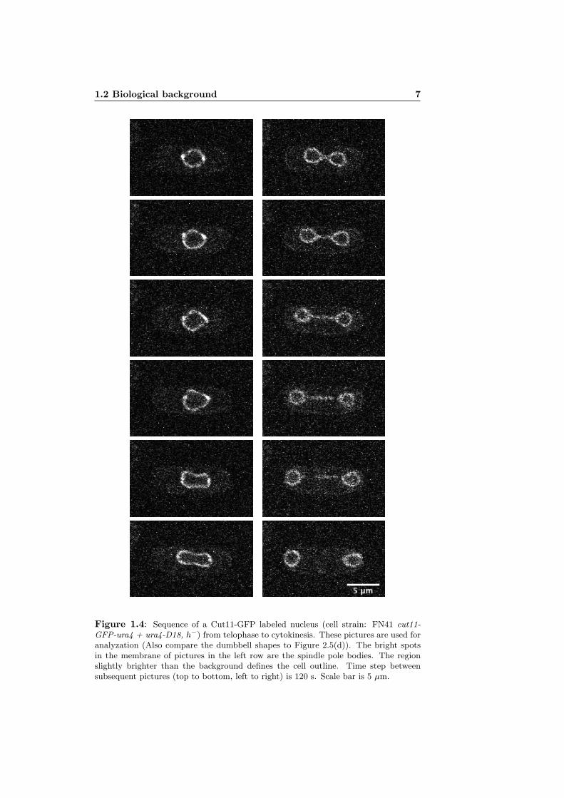
1.2 Biological background 7
Figure 1.4: Sequence of a Cut11-GFP labeled nucleus (cell strain: FN41 cut11-GFP-ura4 + ura4-D18, h−) from telophase to cytokinesis. These pictures are used foranalyzation (Also compare the dumbbell shapes to Figure 2.5(d)). The bright spotsin the membrane of pictures in the left row are the spindle pole bodies. The regionslightly brighter than the background defines the cell outline. Time step betweensubsequent pictures (top to bottom, left to right) is 120 s. Scale bar is 5 µm.
8 Introduction
1.3 Confocal fluorescence microscopy
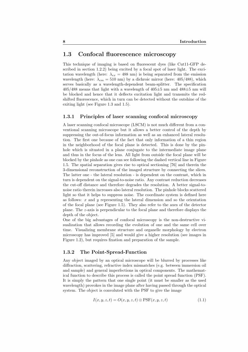
This technique of imaging is based on fluorescent dyes (like Cut11-GFP de-scribed in section 1.2.2) being excited by a focal spot of laser light. The exci-tation wavelength (here: λex = 488 nm) is being separated from the emissionwavelength (here: λem = 510 nm) by a dichroic mirror (here: 405/488), whichserves basically as a wavelength-dependent beam-splitter. The specification405/488 means that light with a wavelength of 405±5 nm and 488±5 nm willbe blocked and hence that it deflects excitation light and transmits the red-shifted fluorescence, which in turn can be detected without the outshine of theexiting light (see Figure 1.3 and 1.5).
1.3.1 Principles of laser scanning confocal microscopy
A laser scanning confocal microscope (LSCM) is not much different from a con-ventional scanning microscope but it allows a better control of the depth bysuppressing the out-of-focus information as well as an enhanced lateral resolu-tion. The first one because of the fact that only information of a thin regionin the neighborhood of the focal plane is detected. This is done by the pin-hole which is situated in a plane conjugate to the intermediate image planeand thus in the focus of the lens. All light from outside the focal plane will beblocked by the pinhole as one can see following the dashed vertical line in Figure1.5. The spatial separation gives rise to optical sectioning [76] and therein the3-dimensional reconstruction of the imaged structure by connecting the slices.The latter one - the lateral resolution - is dependent on the contrast, which inturn is dependent on the signal-to-noise ratio. Any contrast reduction decreasesthe cut-off distance and therefore degrades the resolution. A better signal-to-noise ratio therein increases also lateral resolution. The pinhole blocks scatteredlight so that it helps to suppress noise. The coordinate system is defined hereas follows: x and y representing the lateral dimension and so the orientationof the focal plane (see Figure 1.5). They also refer to the axes of the detectorplane. The z-axis is perpendicular to the focal plane and therefore displays thedepth of the object.One of the big advantages of confocal microscopy is the non-destructive vi-sualization that allows recording the evolution of one and the same cell overtime. Visualizing membrane structure and organelle morphology by electronmicroscopy has improved [5] and would give a higher resolution (see images inFigure 1.2), but requires fixation and preparation of the sample.
1.3.2 The Point-Spread-Function
Any object imaged by an optical microscope will be blurred by processes likediffraction, scattering, refractive index mismatches (e.g. between immersion oiland sample) and general imperfections in optical components. The mathemat-ical function to describe this process is called the point spread function (PSF).It is simply the pattern that one single point (it must be smaller as the usedwavelength) provokes in the image plane after having passed through the opticalsystem. The object is convoluted with the PSF to give the image
I(x, y, z, t) = O(x, y, z, t)⊗ PSF(x, y, z, t) (1.1)

1.3 Confocal fluorescence microscopy 9
beampath in a confocal microscope
detector
laser
objective
sample
beam splitter
pinhole
lenslens
focal plane
Figure 1.5: Principal beamline: The exciting laser light (green) is deflected bythe beam splitter and focused at the sample in the focal plane. The dye is excitedand emits light of longer wavelength(red) than the exciting one. The emitted light istransmitted by the beam splitter and detected after passing the pinhole. Note thatthe specimen has to be moved for scanning the sample in the focal plane. Anotherpossibility would be to invoke a deflection mirror that enables the focus to be moved.Drawing from MTZ Light Microscopy Facility, Dresden, Germany.
where I is the image and O the object. The symbol ⊗ denotes convolution of Oand PSF . If we take the Fourier transform F of equation (1.1), the ⊗ becomesan ordinary multiplication
F [I(x, y, z, t)] = F [O(x, y, z, t)] · F [PSF(x, y, z, t)] (1.2)
This is an important feature for image deconvolution. The full-width-half-maximum (FWHM) of the PSF in lateral (Wx,y) and axial direction (Wz) canbe approximated by [56]
Wx = Wy =0.47 · λη sin(α)
and Wz =0.44 · λ
η sin2(α/2)(1.3)
where λ is the wavelength of the used light (here: λem = 510 nm), η therefractive index of the medium between the specimen and the objective (here:immersion oil η = 1.518) and α = sin−1(NA/η) the semi-aperture angle of theobjective. (NA denotes the numerical aperture.) With these values specified weget
Wx = Wy ≈ 177 nm and Wz ≈ 544 nm
The lateral extension is the same in x- and y-direction as the PSF is rotationallysymmetric about the z-axis. In z-direction, the main intensity is distributedellipsoidal with the semi-major axis aligned (prolate).

10 Introduction
1.3.3 Microscope setup
Olympus Fluoview
The microscope used in this work is an Olympus FV-1000. It is an invertedlaser scanning confocal microscope. An oil immersion objective (ULSAPO 60x)with NA = 1.35 was used. The immersion oil refractive index is η = 1.518. Anargon laser with a wavelength of 488 nm was choosen to excite the fluorophore.In this setup the diameter of the pinhole is 105 µm. Together with the objectivemagnification (60x), the system magnification (3.82 - provided by Olympus engi-neers) the backprojected pinhole radius is calculated to≈229 nm. Backprojectedmeans the size of the pinhole as it appears in the specimen plane: the physicalpinhole size rphys divided by the total magnification of the detection system.This total magnification is the product of the (usually variable) objective magni-fication times a fixed internal magnification: rbackfocal = rphys
mobj ·msys where mobj
is the magnification factor of the objective and msys is the fixed magnificationof the system (see also: http://support.svi.nl/wiki/NyquistCalculator).This calculated backprojected pinhole radius matches with the optical resolution(Rayleigh criterion) of about 200 nm to get best possible results. The Rayleighcriterion shortly displays the necessary separation of two self-luminous pointsources such that their diffraction patterns show a detectable drop in intensitybetween them.The detector is a photomultiplier tube (PMT) sensitive to light of 494 - 545 nm.Binning of registered photons into a raster of pixels makes it reasonable to di-vide the optical resolution by at least a factor of about 2 to avoid the loss ofinformation. This is explained by the Nyquist sampling rate that roughly says:If you want to convert an analog signal into a digitized one, you have to use asampling rate of at least two times the highest frequency of the actual analogsignal. The chosen pixel resolution of 98 nm/pixel in both directions (x andy) satisfies the criterion. Any much finer sized raster would not improve theamount of information and a coarser one would produce undersampling, reduc-ing the recorded brightness of small features. As the image size here is 120 by192 pixels it represents 11.7 by 18.8 µm.Z-resolution (the distance between subsequent z-stacks) is 300 nm. As 14 dif-ferent z-slices are taken, the overall scanning depth is 3.9 µm, slicing the wholenucleus (the average size of a S. pombe nucleus is 7-15 µm in length and around4 µm in diameter [29]). One could blame for oversampling as the PSF in z-direction was calculated to 544 nm (using equation 1.3) and subsequently thereis always a part of information from neighboring z-stacks in the actual slice.But oversampling is not critical and only increases the amount of data - assum-ing that it is not an exaggerated oversampling, because this would imply eithermore damage to the dye by longer excitation or fewer photons/pixel - explainedby the sampling speed.Sampling speed in turn is a critical value and always a compromise betweensignal quality and bleaching. Usually, the longer the dwell time on a particularpixel, the more signal will be detected and the less it will be distorted by Pois-son noise. On the other side the longer the laser focus excites a certain region,the more bleaching will occur and the worse the signal will become over time.The used 12.5 µs/pixel is such a compromise. Time intervals between subse-quent series of z-stacks are chosen to be ∆t = 2 min. This is a good balance

1.3 Confocal fluorescence microscopy 11
between the recording of all the different shapes of the nucleus and minimiza-tion of photodamage for not losing so much signal quality over time. 590 µWis the optimal laser power calculated to balance between fluorophore excita-tion and background-increasing events (autofluorescence, Raman and Rayleighscattering) [57].
Zeiss UV
Most of the features are similar to the Olympus setup, that only the mainsettings are mentioned.
• Objective: Plan Apochromat 63x/1.4 oil DIC
• Excitation wavelength 488 nm
• Longpass filter 505
• Pinhole radius: 104 µm
• Pixel time 5-6 µs
• x, y-resolution: mostly 80 nm
• z-resolution: 300 nm
1.3.4 Sample preparation
The used S. pombe strain (FN41 cut11-GFP-ura4 + ura4-D18, h−) was cul-tured and bountiful provided by I. Raabe (Tolic-Nørrelykke group, MPI-CBG,Germany). The EMM (Edinburgh Minimal Medium; for details see Appendixon page 53) is used to nourish the culture both in the case of solid and liquidculturing.First, 4-5 ml of liquid EMM is inoculated by taking a swab of a solid culturedstrain. This so called preculture is incubated at 25 for 24 hours. Then, ≈1 mlof the preculture is used to inoculate 50 ml of a fresh EMM, that is subsequentlyincubated for another 24 hours. This culture now is used to prepare the sample.Lectin (2 mg/ml) is given on a coverslip (No. 1.5) and dried. This serves as aglue to fix the yeast cells. Silikon at the rim of the coverslip is used to attach itto the previously prepared Microwell dish (35 mm petri dish, 10 mm microwell)in a way, that the glutinous part of the coverslip is freely accessible through thehole in the bottom of the dish. The silicon seals the gap between coverslip anddish, so that the final culture can be dripped onto without leaking. After sed-imentation for about 10 minutes, the not yet settled cells are carefully washedaway. The dish is filled with fresh EMM during all the time of imaging.


2
Methods
2.1 Fourier series and Fourier expansion
An arbitrary complicated shape is not trivial to describe without using a largenumber of parameters or losing generality. Polygon or chain code approxima-tions would require a lot of segments to describe a general contour. To overcomethis problem, we use the Fourier expansion up to frequencies where the ampli-tudes are negligible. We developed a tool (that we will call 2d-contour-explorer)to create significantly different shapes by manipulating very few parameters.Obvious not completely closed contours as they may occur in confocal imagesdue to a partially bad fluorescence signal or imperfect labeling will be automat-ically represented as closed structures, making it an interesting kind of descrip-tion for life sciences. Even if there are only a few dots along the contour, themathematical description by Fourier series (FS) contains all the intermediatepoints due to the use of continuous basis functions (see next section).
2.1.1 Introduction to Fourier series
Every regular (without singularities), periodic function f(x) can be representedby a infinite sum of sines and cosines (the basis functions).
f(x) =a0
2+∞∑n=1
[an cos(n · x) + bn sin(n · x)] (2.1)
where the coefficients calculate to
an =1π
∫ π
−πf(x) cos(n·x)dx bn =
1π
∫ π
−πf(x) sin(n·x)dx and a0 =
1π
∫ π
−πf(x)dx
These are the so called Fourier coefficients. The only limitations that have tobe set on f(x)are:
1. f(x) has only a finite number of maxima and minima
2. f(x) has only a finite number of (finite) discontinuities
3. f(x) must be 2π-periodic
14 Methods
For even functions bn = 0 and the series reduces to
feven(x) =a0
2+∞∑n=1
an cos(n · x)
likewise for odd functions, where an = 0, it becomes
fodd(x) =∞∑n=1
bn sin(n · x)
The derivatives are easily calculated, as one can see e.g. for the first derivative
f ′(x) =df(x)dx
= 0 +∞∑n=1
[nbn cos(n · x)− an sin(n · x)] (2.2)
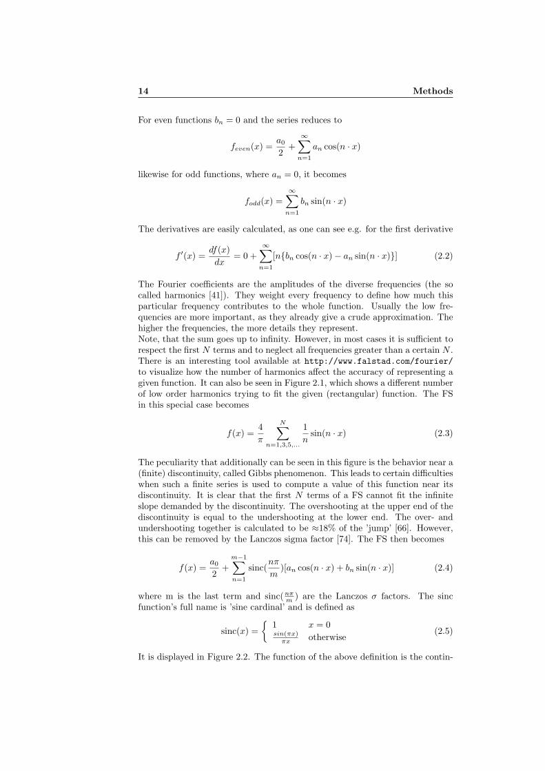
The Fourier coefficients are the amplitudes of the diverse frequencies (the socalled harmonics [41]). They weight every frequency to define how much thisparticular frequency contributes to the whole function. Usually the low fre-quencies are more important, as they already give a crude approximation. Thehigher the frequencies, the more details they represent.Note, that the sum goes up to infinity. However, in most cases it is sufficient torespect the first N terms and to neglect all frequencies greater than a certain N .There is an interesting tool available at http://www.falstad.com/fourier/to visualize how the number of harmonics affect the accuracy of representing agiven function. It can also be seen in Figure 2.1, which shows a different numberof low order harmonics trying to fit the given (rectangular) function. The FSin this special case becomes
f(x) =4π
N∑n=1,3,5,...
1n
sin(n · x) (2.3)
The peculiarity that additionally can be seen in this figure is the behavior near a(finite) discontinuity, called Gibbs phenomenon. This leads to certain difficultieswhen such a finite series is used to compute a value of this function near itsdiscontinuity. It is clear that the first N terms of a FS cannot fit the infiniteslope demanded by the discontinuity. The overshooting at the upper end of thediscontinuity is equal to the undershooting at the lower end. The over- andundershooting together is calculated to be ≈18% of the ’jump’ [66]. However,this can be removed by the Lanczos sigma factor [74]. The FS then becomes
f(x) =a0
2+m−1∑n=1
sinc(nπ
m)[an cos(n · x) + bn sin(n · x)] (2.4)
where m is the last term and sinc(nπm ) are the Lanczos σ factors. The sincfunction’s full name is ’sine cardinal’ and is defined as
sinc(x) =
1 x = 0sin(πx)πx otherwise
(2.5)
It is displayed in Figure 2.2. The function of the above definition is the contin-

2.1 Fourier series and Fourier expansion 15
0 1 2 3 4 5 6 7!1.5
!1
!0.5
0
0.5
1
1.5
x
f(x
)Gibbs phenomenon
Square waveN = 1N = 3N = 5N = 29
Figure 2.1: As explained in the text, there is a natural over- and undershooting atthe discontinuities (the Gibbs phenomenon), even if high frequencies are included inthe Fourier series (FS). All the functions are plotted from 0 to 2π. The black line isthe given rectangular function. The colored graphs show the different adaption levelby using equation (2.3) with different values for N . In red, only the first harmonicis considered and thus it shows the ordinary sine function. The more harmonics areincluded, the better the FS fits to the original function.
!6 !4 !2 0 2 4 6!0.4
!0.2
0
0.2
0.4
0.6
0.8
1
x
sinc
(x)
sinc function
Figure 2.2: The sine cardinal (sinc)function as defined in equation (2.5) dis-played from −2π to 2π. If it would bedefined like sinc(x) = sin(x)
xfor x 6= 0
(and sinc(x) = 1 for x = 0), it would turnout that sinc(x) ≡ j0(x) (spherical Besselfunction of the first kind).
0 1 2 3 4 5 6 7!1.5
!1
!0.5
0
0.5
1
1.5
x
f(x
)
Lanczos ! factor
Square waveN = 5N = 29
Figure 2.3: Removing of over- and un-dershooting by Lanczos σ factors (equa-tion (2.4) is used). Comparing the graphsin this Figure with the corresponding onesin Figure 2.1 shows the much better adap-tion to the given function. (The rectan-gular function (black) is the same in bothfigures.)
16 Methods
uous inverse Fourier transform of a rectangular pulse of width 2π and height 1.There are alternative definitions (see [74]), but in any case it is closely relatedto the spherical Bessel function of the first kind j0(x).A different but equivalent description [8] of the FS is
f(x) =a0
2+∞∑n=1
An sin(n · x+ ϕn) (2.6)
where in this case An =√a2n + b2n and tanϕn = an
bn. If we represent the series
in its extended complex form (by replacing cos(n · x) = 12 (einx + e−inx) and
sin(n · x) = 12i (e
inx − e−inx) in equation (2.1) it becomes
f(x) = c0 +∞∑n=1
(cneinx + c−ne−inx) =
∞∑n=−∞
cneinx (2.7)
where i is the complex number and cn = 12π
∫ π−π f(x)e−inxdx, n = 0,±1,±2, ....
Note that the coefficients can be written as
cn =
1
2π
∫ π−π f(x)[cos(n · x) + i sin(n · x)]dx = 1
2 (a−n + ib−n) for n < 01
2π
∫ π−π f(x)dx = 1
2a0 for n = 01
2π
∫ π−π f(x)[cos(n · x)− i sin(n · x)]dx = 1
2 (an − ibn) for n > 0
Moreover the cn are the basis for the Fourier transform, which is obtainedby denoting cn = 1
L
∫ L/2−L/2 f(x)e−i(
2πnL x)dx and converting the discrete cn to a
continuous F (k) by letting the length of the periodic function L −→ ∞, whileletting n
L −→ k.
2.1.2 Fourier series representation
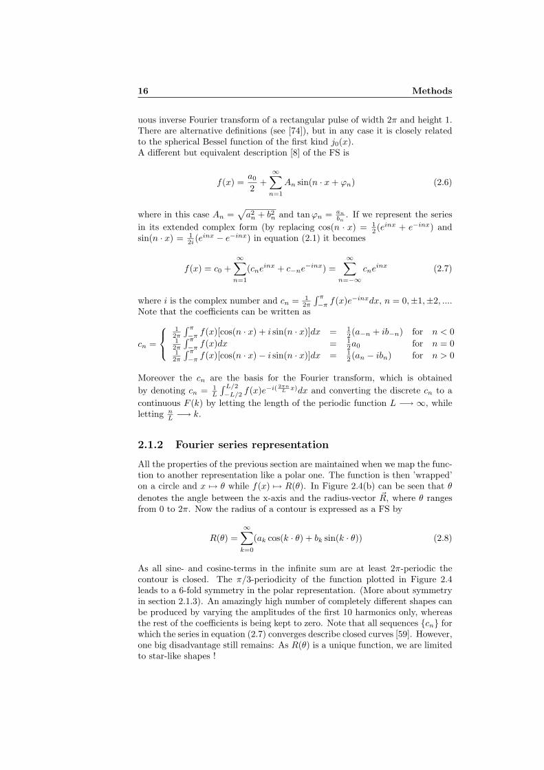
All the properties of the previous section are maintained when we map the func-tion to another representation like a polar one. The function is then ’wrapped’on a circle and x 7→ θ while f(x) 7→ R(θ). In Figure 2.4(b) can be seen that θdenotes the angle between the x-axis and the radius-vector ~R, where θ rangesfrom 0 to 2π. Now the radius of a contour is expressed as a FS by
R(θ) =∞∑k=0
(ak cos(k · θ) + bk sin(k · θ)) (2.8)
As all sine- and cosine-terms in the infinite sum are at least 2π-periodic thecontour is closed. The π/3-periodicity of the function plotted in Figure 2.4leads to a 6-fold symmetry in the polar representation. (More about symmetryin section 2.1.3). An amazingly high number of completely different shapes canbe produced by varying the amplitudes of the first 10 harmonics only, whereasthe rest of the coefficients is being kept to zero. Note that all sequences cn forwhich the series in equation (2.7) converges describe closed curves [59]. However,one big disadvantage still remains: As R(θ) is a unique function, we are limitedto star-like shapes !
2.1 Fourier series and Fourier expansion 17
0 0.52 1.04 1.57 2.09 2.61 3.14 3.66 4.19 4.71 5.23 5.76 6.280
0.2
0.4
0.6
0.8
1
1.2
x
f(x
)
f (x) = 0.2 · sin(6 · x) + 1f (x = !/6)
(a) Usual cartesian representation
0.5
1
1.5
30
210
60
240
90
270
120
300
150
330
180 0
R(!) = 0.2 · sin(6 · !) + 1
x
y
"R(! = #/6)
(b) Mapped polar representation
Figure 2.4: In both figures the same function is plotted. In figure (a) it is representedin cartesian coordinates, whereas in figure(b) it is mapped to polar coordinates. Thefunction value f becomes the length of the ~R-vector and the x-coordinate the anglebetween the x-axis and the ~R-vector. The angle is denoted counterclockwise. Thegraph in figure (b) is closed, due to the 2π-periodicity of the function. The additionalπ/3-periodicity causes the observed 6-fold symmetry. A cartesian coordinate systemis superimposed to the polar coordinate system.
2.1.3 Fourier coordinate expansion
To create non-star-like shapes we expand x and y separately in a completeFourier expansion and then represent every point of the contour with a pair(x, y). Both x and y depend on a parameter t that is to be considered differentfrom the angle θ as defined for equation (2.8). One can think of a parametric2-dimensional vector ~p, where x and y are the components
~p(t) =(x(t)y(t)
)(2.9)
The parameter t then can be seen as the arc length (see ’Concept of a Curve’[49]), or more advanced: The time when we trace out the way along the curve(yet at constant velocity). Assuming that we prevent self-intersection, everypair (x(t), y(t)) determines a unique point on the perimeter for every differentt. The two expansions that we have to consider now are
x(t) =∞∑k=0
(Axk cos(k · t) +Bxk sin(k · t)) (2.10)
y(t) =∞∑k=0
(Ayk cos(k · t) +Byk sin(k · t)) (2.11)
with the Axk, Bxk , Ayk and Byk being the coefficients. The upper indices are notto be mistaken for exponents ! In the following we will always refer to thisparametric expansion of equations (2.10) and (2.11) and their coefficients.All coefficients k ≥ 2 can be normalized by the ’radius of the 1st harmonic circle’(√
[Ax,y1 ]2 + [Bx,y1 ]2 respectively for x and y) to get relative amplitudes, but wejust keep in mind, that we use absolute values.

18 Methods
Szekely et al. [68] used the same approach for the parameterization of 2-Dcontours in their segmentation of midsagittal MR (magnetic resonance) images.They used it as a basis for Fourier snakes, whereas we will use a different method(see section 2.4). Kuhl and Giardina [45] in turn used the Fourier series expan-sion successfully in combination with chain-encoded contours. They thereforeused well defined contours where subsequent pixels are 8-connected, so that it isunstated how the procedure will deal with noise. (In 2-D, pixels are 8-connectedif their edges or corners touch and so subsequent pixels are connected along thehorizontal, vertical or diagonal direction.) A different approach worked out byGielis [28] is the ’Superformula’ which is based on a tuned ellipsoidal equation.It is also a powerful tool regarding the creation of diverse shapes by changingfew parameters, but without intersection it cannot create closed non-starlikecontours.
Simple shapes
To show the simplicity of obtaining very basic shapes like a circle or an ellipse,see some examples in Table 2.1. Already here it becomes clear that there is
Ax1 Bx1 Ay1 By1Circle 1 0 0 1Ellipse oblate 1 0 0 < 1Ellipse prolate < 1 0 0 1
Table 2.1: The most basic shapes and their coefficients. All higher harmonics (k ≥ 2)are equal to zero. This is just one example, there are other possible combinations tocreate the very same shapes. Changing the values of Ax
1 ↔ Bx1 and Ay
1 ↔ By1
for example will not change the resulting shapes (but the orientation of the tangentvector → see chapter 2.3.2). Also an arbitrary chosen k 6= 1 is valid, when all otherharmonics except the chosen one are set to zero. In this case the same shape will bedrawn k times.
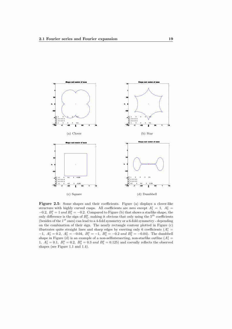
not only one set of coefficients unambiguously connected to a particular shape.In the regarded case of high symmetric shapes (circle and ellipse) exists evenan infinite number of possible sets that describe the identical shapes ! Fixingthe values of the amplitudes in Table 2.1 makes it clear. The subindex k canbe chosen arbitrarily without changing the resulting shape. Like in the casek = 1 (which is displayed in the table), where all other amplitudes k 6= 1 musthave been equal to zero, we just have to set all amplitudes to zero that are notcorresponding to the kth harmonic that has been chosen. The circle or ellipsewill then be drawn k times.A few remarkable things can be seen in the slightly less basic shapes displayedin Figure 2.5. First, cusps and spicules may arise already at low harmonics,resulting in highly curved regions. Second, almost straight lines can be producedthat are connected by sharp edges. Note that only harmonics k ≤ 5 are used.Third, there is the ’proof’ that non-starlike shapes are easily obtained. Remarksabout the symmetry will be made in the next section.
2.1 Fourier series and Fourier expansion 19
!1.5 !1 !0.5 0 0.5 1 1.5!1.5
!1
!0.5
0
0.5
1
1.5
Akx: −1 0 0 0 0
Bkx: 0 0 0 0 0
Aky: 0 0 0 0 0
Bky: 0 0 0 0 0
x
y
Shape and center of mass
shapecenter of perimeter
!1.5 !1 !0.5 0 0.5 1 1.5!1.5
!1
!0.5
0
0.5
1
1.5
Akx: −1 0 0 0 0
Bkx: 0 0 0 0 0
Aky: 0 0 0 0 0
Bky: −1 0 0 0 0
x
y
Shape and center of mass
shapecenter of perimeter
!1.5 !1 !0.5 0 0.5 1 1.5!1.5
!1
!0.5
0
0.5
1
1.5
Akx: −1 0 0.2 0 0
Bkx: 0 0 0 0 0
Aky: 0 0 0 0 0
Bky: −1 0 0 0 0
x
y
Shape and center of mass
!1.5 !1 !0.5 0 0.5 1 1.5!1.5
!1
!0.5
0
0.5
1
1.5
Akx: −1 0 0.2 0 0
Bkx: 0 0 0 0 0
Aky: 0 0 0 0 0
Bky: −1 0 −0.2 0 0
x
y
Shape and center of mass
!1.5 !1 !0.5 0 0.5 1 1.5!1.5
!1
!0.5
0
0.5
1
1.5
Akx: −1 0 0.2 0 −0.035
Bkx: 0 0 0 0 0
Aky: 0 0 0 0 0
Bky: −1 0 −0.2 0 0
x
y
Shape and center of mass
!1.5 !1 !0.5 0 0.5 1 1.5!1.5
!1
!0.5
0
0.5
1
1.5
Akx: −1 0 0.2 0 −0.035
Bkx: 0 0 0 0 0
Aky: 0 0 0 0 0
Bky: −1 0 −0.2 0 −0.035
x
y
Shape and center of mass
!1.5 !1 !0.5 0 0.5 1 1.5!1.5
!1
!0.5
0
0.5
1
1.5
Akx: 1 0 0.2 0 −0.035
Bkx: 0 0 0 0 0
Aky: 0 0 0 0 0
Bky: −1 0 −0.2 0 −0.035
x
y
Shape and center of mass
!1.5 !1 !0.5 0 0.5 1 1.5!1.5
!1
!0.5
0
0.5
1
1.5
Akx: 1 0 0.2 0 −0.035
Bkx: 0 0 0 0 0
Aky: 0 0 0 0 0
Bky: 1 0 −0.2 0 −0.035
x
y
Shape and center of mass
!1.5 !1 !0.5 0 0.5 1 1.5!1.5
!1
!0.5
0
0.5
1
1.5
Akx: 1 0 0 0 −0.035
Bkx: 0 0 0 0 0
Aky: 0 0 0 0 0
Bky: 1 0 −0.2 0 −0.035
x
y
Shape and center of mass
!1.5 !1 !0.5 0 0.5 1 1.5!1.5
!1
!0.5
0
0.5
1
1.5
Akx: 1 0 0 0 −0.035
Bkx: 0 0 0 0 0
Aky: 0 0 0 0 0
Bky: 1 0 0 0 −0.035
x
y
Shape and center of mass
!1.5 !1 !0.5 0 0.5 1 1.5!1.5
!1
!0.5
0
0.5
1
1.5
Akx: 1 0 0 0 −0.2
Bkx: 0 0 0 0 0
Aky: 0 0 0 0 0
Bky: 1 0 0 0 −0.035
x
y
Shape and center of mass
!1.5 !1 !0.5 0 0.5 1 1.5!1.5
!1
!0.5
0
0.5
1
1.5
Akx: 1 0 0 0 −0.2
Bkx: 0 0 0 0 0
Aky: 0 0 0 0 0
Bky: 1 0 0 0 0
x
y
Shape and center of mass
!1.5 !1 !0.5 0 0.5 1 1.5!1.5
!1
!0.5
0
0.5
1
1.5
Akx: 1 0 0 0 −0.2
Bkx: 0 0 0 0 0
Aky: 0 0 0 0 0
Bky: 1 0 0 0 −0.2
x
y
Shape and center of mass
(a) Clover
!1.5 !1 !0.5 0 0.5 1 1.5!1.5
!1
!0.5
0
0.5
1
1.5
Akx: −1 0 0 0 0
Bkx: 0 0 0 0 0
Aky: 0 0 0 0 0
Bky: 0 0 0 0 0
xy
Shape and center of mass
shapecenter of perimeter
!1.5 !1 !0.5 0 0.5 1 1.5!1.5
!1
!0.5
0
0.5
1
1.5
Akx: −1 0 0 0 0
Bkx: 0 0 0 0 0
Aky: 0 0 0 0 0
Bky: −1 0 0 0 0
xy
Shape and center of mass
shapecenter of perimeter
!1.5 !1 !0.5 0 0.5 1 1.5!1.5
!1
!0.5
0
0.5
1
1.5
Akx: −1 0 0.2 0 0
Bkx: 0 0 0 0 0
Aky: 0 0 0 0 0
Bky: −1 0 0 0 0
xy
Shape and center of mass
!1.5 !1 !0.5 0 0.5 1 1.5!1.5
!1
!0.5
0
0.5
1
1.5
Akx: −1 0 0.2 0 0
Bkx: 0 0 0 0 0
Aky: 0 0 0 0 0
Bky: −1 0 −0.2 0 0
xy
Shape and center of mass
!1.5 !1 !0.5 0 0.5 1 1.5!1.5
!1
!0.5
0
0.5
1
1.5
Akx: −1 0 0.2 0 −0.035
Bkx: 0 0 0 0 0
Aky: 0 0 0 0 0
Bky: −1 0 −0.2 0 0
xy
Shape and center of mass
!1.5 !1 !0.5 0 0.5 1 1.5!1.5
!1
!0.5
0
0.5
1
1.5
Akx: −1 0 0.2 0 −0.035
Bkx: 0 0 0 0 0
Aky: 0 0 0 0 0
Bky: −1 0 −0.2 0 −0.035
xy
Shape and center of mass
!1.5 !1 !0.5 0 0.5 1 1.5!1.5
!1
!0.5
0
0.5
1
1.5
Akx: 1 0 0.2 0 −0.035
Bkx: 0 0 0 0 0
Aky: 0 0 0 0 0
Bky: −1 0 −0.2 0 −0.035
xy
Shape and center of mass
!1.5 !1 !0.5 0 0.5 1 1.5!1.5
!1
!0.5
0
0.5
1
1.5
Akx: 1 0 0.2 0 −0.035
Bkx: 0 0 0 0 0
Aky: 0 0 0 0 0
Bky: 1 0 −0.2 0 −0.035
xy
Shape and center of mass
!1.5 !1 !0.5 0 0.5 1 1.5!1.5
!1
!0.5
0
0.5
1
1.5
Akx: 1 0 0 0 −0.035
Bkx: 0 0 0 0 0
Aky: 0 0 0 0 0
Bky: 1 0 −0.2 0 −0.035
xy
Shape and center of mass
!1.5 !1 !0.5 0 0.5 1 1.5!1.5
!1
!0.5
0
0.5
1
1.5
Akx: 1 0 0 0 −0.035
Bkx: 0 0 0 0 0
Aky: 0 0 0 0 0
Bky: 1 0 0 0 −0.035
xy
Shape and center of mass
!1.5 !1 !0.5 0 0.5 1 1.5!1.5
!1
!0.5
0
0.5
1
1.5
Akx: 1 0 0 0 −0.2
Bkx: 0 0 0 0 0
Aky: 0 0 0 0 0
Bky: 1 0 0 0 −0.035
xy
Shape and center of mass
!1.5 !1 !0.5 0 0.5 1 1.5!1.5
!1
!0.5
0
0.5
1
1.5
Akx: 1 0 0 0 −0.2
Bkx: 0 0 0 0 0
Aky: 0 0 0 0 0
Bky: 1 0 0 0 0
xy
Shape and center of mass
!1.5 !1 !0.5 0 0.5 1 1.5!1.5
!1
!0.5
0
0.5
1
1.5
Akx: 1 0 0 0 −0.2
Bkx: 0 0 0 0 0
Aky: 0 0 0 0 0
Bky: 1 0 0 0 −0.2
xy
Shape and center of mass
!1.5 !1 !0.5 0 0.5 1 1.5!1.5
!1
!0.5
0
0.5
1
1.5
Akx: 1 0 0 0 −0.2
Bkx: 0 0 0 0 0
Aky: 0 0 0 0 0
Bky: 1 0 0 0 0.2
xy
Shape and center of mass
(b) Star
!1.5 !1 !0.5 0 0.5 1 1.5!1.5
!1
!0.5
0
0.5
1
1.5
Akx: −1 0 0 0 0
Bkx: 0 0 0 0 0
Aky: 0 0 0 0 0
Bky: 0 0 0 0 0
x
y
Shape and center of mass
shapecenter of perimeter
!1.5 !1 !0.5 0 0.5 1 1.5!1.5
!1
!0.5
0
0.5
1
1.5
Akx: −1 0 0 0 0
Bkx: 0 0 0 0 0
Aky: 0 0 0 0 0
Bky: −1 0 0 0 0
x
y
Shape and center of mass
shapecenter of perimeter
!1.5 !1 !0.5 0 0.5 1 1.5!1.5
!1
!0.5
0
0.5
1
1.5
Akx: −1 0 0.2 0 0
Bkx: 0 0 0 0 0
Aky: 0 0 0 0 0
Bky: −1 0 0 0 0
x
y
Shape and center of mass
!1.5 !1 !0.5 0 0.5 1 1.5!1.5
!1
!0.5
0
0.5
1
1.5
Akx: −1 0 0.2 0 0
Bkx: 0 0 0 0 0
Aky: 0 0 0 0 0
Bky: −1 0 −0.2 0 0
x
y
Shape and center of mass
!1.5 !1 !0.5 0 0.5 1 1.5!1.5
!1
!0.5
0
0.5
1
1.5
Akx: −1 0 0.2 0 −0.035
Bkx: 0 0 0 0 0
Aky: 0 0 0 0 0
Bky: −1 0 −0.2 0 0
x
y
Shape and center of mass
!1.5 !1 !0.5 0 0.5 1 1.5!1.5
!1
!0.5
0
0.5
1
1.5
Akx: −1 0 0.2 0 −0.035
Bkx: 0 0 0 0 0
Aky: 0 0 0 0 0
Bky: −1 0 −0.2 0 −0.035
x
y
Shape and center of mass
(c) Square
!1.5 !1 !0.5 0 0.5 1 1.5!1.5
!1
!0.5
0
0.5
1
1.5
Akx: 0 0 0 0 0
Bkx: 0 0 0 0 0
Aky: 0 0 0 0 0
Bky: 0 0 0 0 0
x
y
Shape and center of mass
shape
!1.5 !1 !0.5 0 0.5 1 1.5!1.5
!1
!0.5
0
0.5
1
1.5
Akx: 1 0 0 0 0
Bkx: 0 0 0 0 0
Aky: 0 0 0 0 0
Bky: 0 0 0 0 0
x
y
Shape and center of mass
shapecenter of perimeter
!1.5 !1 !0.5 0 0.5 1 1.5!1.5
!1
!0.5
0
0.5
1
1.5
Akx: 1 0 0 0 0
Bkx: 0 0 0 0 0
Aky: 0 0 0 0 0
Bky: 0.2 0 0 0 0
x
y
Shape and center of mass
shapecenter of perimeter
!1.5 !1 !0.5 0 0.5 1 1.5!1.5
!1
!0.5
0
0.5
1
1.5
Akx: 1 0 0 0 0
Bkx: 0 0 0 0 0
Aky: 0 0 0 0 0
Bky: 0.2 0 0.3 0 0
x
y
Shape and center of mass
!1.5 !1 !0.5 0 0.5 1 1.5!1.5
!1
!0.5
0
0.5
1
1.5
Akx: 1 0 0 0 0.1
Bkx: 0 0 0 0 0
Aky: 0 0 0 0 0
Bky: 0.2 0 0.3 0 0
x
y
Shape and center of mass
!1.5 !1 !0.5 0 0.5 1 1.5!1.5
!1
!0.5
0
0.5
1
1.5
Akx: 1 0 0 0 0.1
Bkx: 0 0 0 0 0
Aky: 0 0 0 0 0
Bky: 0.2 0 0.3 0 0.125
x
y
Shape and center of mass
(d) Dumbbell
Figure 2.5: Some shapes and their coefficients. Figure (a) displays a clover-likestructure with highly curved cusps. All coefficients are zero except Ax
1 = 1, Ax5 =
−0.2, By1 = 1 and By
5 = −0.2. Compared to Figure (b) that shows a starlike shape, theonly difference is the sign of By
5 , making it obvious that only using the 5th coefficients(besides of the 1st ones) can lead to a 4-fold symmetry or a 6-fold symmetry - dependingon the combination of their sign. The nearly rectangle contour plotted in Figure (c)illustrates quite straight lines and sharp edges by exerting only 6 coefficients (Ax
1 =−1, Ax
3 = 0.2, Ax5 = −0.04, By
1 = −1, By3 = −0.2 and By
5 = −0.04). The dumbbellshape in Figure (d) is an example of a non-selfintersecting, non-starlike outline (Ax
1 =1, Ax
5 = 0.1, By1 = 0.2, By
3 = 0.3 and By5 = 0.125) and coevally reflects the observed
shapes (see Figure 1.1 and 1.4).
20 Methods
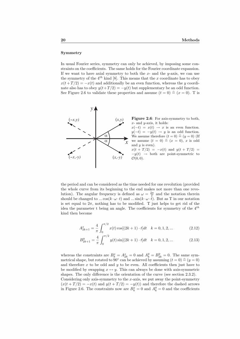
Symmetry
In usual Fourier series, symmetry can only be achieved, by imposing some con-straints on the coefficients. The same holds for the Fourier coordinate expansion.If we want to have axial symmetry to both the x- and the y-axis, we can usethe symmetry of the 4th kind [8]. This means that the x coordinate has to obeyx(t+T/2) = −x(t) and additionally be an even function, whereas the y coordi-nate also has to obey y(t+T/2) = −y(t) but supplementary be an odd function.See Figure 2.6 to validate these properties and assume (t = 0) = (x = 0). T is
αα
(−x,y) (x,y)
(−x,-y) (x,-y)
x
yFigure 2.6: For axis-symmetry to both,x- and y-axis, it holds:x(−t) = x(t) → x is an even function.y(−t) = −y(t) → y is an odd function.We assume therefore (t = 0) b= (y = 0) (Ifwe assume (t = 0) b= (x = 0), x is oddand y is even).x(t + T/2) = −x(t) and y(t + T/2) =−y(t) → both are point-symmetric toO(0, 0).
the period and can be considered as the time needed for one revolution (providedthe whole curve from its beginning to the end makes not more than one revo-lution). The angular frequency is defined as ω = 2π
T and the notation thereinshould be changed to ... cos(k ·ω · t) and ... sin(k ·ω · t). But as T in our notationis set equal to 2π, nothing has to be modified. T just helps to get rid of theidea the parameter t being an angle. The coefficients for symmetry of the 4th
kind then become
Ax2k+1 =4π
∫ π/2
0
x(t) cos[(2k + 1) · t]dt k = 0, 1, 2, ... (2.12)
By2k+1 =4π
∫ π/2
0
y(t) sin[(2k + 1) · t]dt k = 0, 1, 2, ... (2.13)
whereas the constraints are Bxk = Ax2k = 0 and Ayk = By2k = 0. The same sym-metrical shape, but rotated to 90 can be achieved by assuming (t = 0) = (y = 0)and therefore x to be odd and y to be even. All coefficients then just have tobe modified by swapping x↔ y. This can always be done with axis-symmetricshapes. The only difference is the orientation of the curve (see section 2.3.2).Considering only axis-symmetry to the x-axis, we put away the point-symmetry(x(t+ T/2) = −x(t) and y(t+ T/2) = −y(t)) and therefore the dashed arrowsin Figure 2.6. The constraints now are Bxk = 0 and Ayk = 0 and the coefficients
2.1 Fourier series and Fourier expansion 21
calculate to
Axk =2π
∫ π
0
x(t) cos(k · t)dt k = 0, 1, 2, ... (2.14)
Byk =2π
∫ π
0
y(t) sin(k · t)dt k = 0, 1, 2, ... (2.15)
Now let us fix all values of the coefficients and only change their signs. Considerthe case: |Ax1 | = 1, |Ax5 | = 0.2, |By1 | = 1 and |By5 | = 0.2, whereas all other coeffi-cients are zero. Denote the signs of the four nonzero-coefficients in a quadrupleaccording to the order specified.(+,−,+,−) ; (−,+,−,+) ; (−,+,+,−) ; (+,−,−,+) all give the clover-likeshape in Figure 2.5(a) and(+,+,+,+) ; (−,−,−,−) ; (+,+,−,−) ; (−,−,+,+) lead to the same shaperotated by 45 (half of the angle of its 4-fold symmetry).(−,+,+,+) ; (+,−,−,−) ; (+,−,+,+) ; (−,+,−,−) in contrast result in thestarlike structure of Figure 2.5(b) and as expected(+,+,+,−) ; (−,−,−,+) ; (+,+,−,+) ; (−,−,+,−) is the same star rotatedby 30.If |Ax4 | = 0.2 and |By4 | = 0.2 are chosen to be nonzero instead of |Ax5 | and |By5 |,the resulting 3-fold symmetric ’clover’ will behave similar regarding the first andsecond set of quadruples but rotate to 60 and therein half of the angle of its3-fold symmetry. The last and the second last set of quadruples now leads to a5-fold-symmetric ’star’ and consequently to a 36 rotation.Slicing the nuclear envelope that will be described here in its middle section -which therein contains the long axis - leads to a 2-fold symmetric contour (ne-glect the orbital shape) and in any case there is a certain similarity to Cassiniovals or toric sections (when the torus is cut by a plane parallel to its rotationalaxis). Hence, instead of using common Cartesian coordinates one may thinkof using Bipolar coordinates [24] to describe the shape. But this should notsimplify things, because in either way there are two variables to fix for defininga particular point. The transformation from Cartesian coordinates to Bipolarcoordinates is unique when the x-axis-symmetric case is considered and henceonly positive y-values for example.
2.1.4 Meaning of the coefficients
The interpretation of the coefficients is an interesting subject. A possible visual-ization are elliptic approximations to a contour based on the system of Ptolemy’sepicycles like in [45]. For an interactive tool about epicycles see http://physics.syr.edu/courses/java/demos/kennett/Epicycle/Epicycle.htmlFirst, we consider curves in two dimensions. This is based on [49] and un-published material of J. Howard (MPI-CBG, Dresden, Germany). Having aregular parametric representation ~p(t) like in equation (2.9), the time derivativecalculates to
~p(t)′ =d~p
dt= lim
∆t→0
~p(t+ ∆t)− ~p(t)∆t
= ~t(t)|~p ′| = v(t) · ~t(t) (2.16)
where ~t(t) is the unit tangent vector (pointing in the direction of travel) andv(t) its magnitude (which can be seen as the speed). The faster the speed, the

22 Methods
more distant are subsequent ’points’ when they are marked at a constant timeinterval while going along the curve. Thinking in terms of intensity or bright-ness: The slower the speed, the brighter the curve.Herein lies the key advantage of such a parameterization: Additionally to defin-ing a curve, it also comprises its intensity and therein includes the descriptionof shapes with non-uniform intensity like they may occur in biological, stainedsamples due to some intrinsic gradient or samples with imperfect labeling.Using a representation in terms of the arc length, we come to a natural represen-tation, where |d~p(s)ds | = 1. This means equidistant ’points’ and therein uniformlydistributed brightness of the curve. Inversely, curves of speed |v| = 1 are called’parameterized by arc length’ [31]. Note that if the arc length is defined as
s = s(t) =∫ t
t0
∣∣∣∣d~pdt∣∣∣∣ dt (2.17)
then ~p(t(s)) is also a natural representation and therefore no squeezing norstretching of the curve occurs. The reparameterization ~p(s) = ~p(t(s)) then justyields
~t(s) =d~p(s)ds∣∣∣ ~p(s)ds
∣∣∣ =d~p(s)ds
=d~p(t(s))ds
=d~p(t)dt
dt
ds=
d~p(t)dtdsdt
=d~p(t)dt∣∣∣d~p(t)dt
∣∣∣ =~p(t)′
v(t)= ~t(t) (2.18)
provided that the speed v(t) is always positive (⇒ t(s) can be inverted ⇒dtds
∣∣t(s)
= [ dsdt∣∣s(t)
]−1 ). Due to the positive v, the curves have the same ori-entation.The average of a function f is defined as
〈f〉t =1
b− a
∫ b
a
f(t)dt (2.19)
When we weight every increment of arc length by the intensity of the curvei(t) = 1
v(t) = dtds we get
1∆t
t0+∆t∫t0
f(t)dt =1
s0(t)+∆s∫s0(t)
dtdsds
s0(t)+∆s∫s0(t)
f(s)dt
dsds (2.20)
whereas, when we weight by both the brightness and the amount of arc lengthwithin the incrementing angle (and therefore by the overall curve material withinthat angle) we obtain
1∆t
t0+∆t∫t0
f(t)dt =1
Θ0(t)+∆Θ∫Θ0(t)
dtds
dsdΘdΘ
Θ0(t)+∆Θ∫Θ0(t)
f(Θ)dt
ds
ds
dΘdΘ (2.21)
Now back to the coefficients of the Fourier coordinate expansion. For the zeroorder coefficients (also called the DC components) we have
Ax0 =1
2π
∫ 2π
0
x(t)dt = 〈x〉t and Ay0 =1
2π
∫ 2π
0
y(t)dt = 〈y〉t (2.22)
2.2 The 2-d-contour-explorer 23
so that they represent the coordinates of the center of mass. For a contour ofuniform intensity, paramtererized by the arc length it is also the center of theperimeter. For higher order coefficients it yields
Axk =1
2π
∫ 2π
0
x(t) cos(k · t)dt = 〈x(t) cos(k · t)〉t (2.23)
Bxk =1
2π
∫ 2π
0
x(t) sin(k · t)dt = 〈x(t) sin(k · t)〉t (2.24)
and likewise for Ayk and Byk . These higher order coefficients correspond to theclosest fit in the least squares sense. For the best fit ellipse for example
Ω2(Ax0 , Ax1 , B
x1 , A
y0, A
y1, B
y1 ) =
12π
∫ 2π
0
[x(t)−Ax0 −Ax1 cos(k · t)−Bx1 sin(k · t)]2
+ [y(t)−Ay0 −Ay1 cos(k · t)−By1 sin(k · t)]2
dt (2.25)
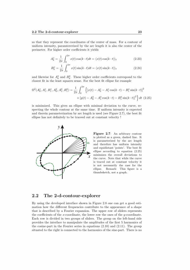
is minimized. This gives an ellipse with minimal deviation to the curve, re-specting the whole contour at the same time. If uniform intensity is expectedand therein parameterization by arc length is used (see Figure 2.7), the best fitellipse has not definitely to be traceed out at constant velocity !
x
y
ds
Figure 2.7: An arbitrary contouris plotted as a green, dashed line. Itis parameterized by the arc lengthand therefore has uniform intensityand equidistant ’points’. The best fitellipse according to equation (2.25)minimizes the overall deviations tothe curve. Note that while the curveis traced out at constant velocity itis not necessarily the case for theellipse. Remark: This figure is athumbsketch, not a graph.
2.2 The 2-d-contour-explorer
By using the developed interface shown in Figure 2.8 one can get a good esti-mation how the different frequencies contribute to the appearance of a shapethat is described by a Fourier expansion. The upper row of sliders representsthe coefficients of the x-coordinate, the lower row the ones of the y-coordinate.Each row is divided in two groups of sliders. The group on the left-hand sideprovides the interface to manipulate the amplitudes of the first 5 harmonics ofthe cosine-part in the Fourier series in equations (2.10) and (2.11). The groupsituated to the right is connected to the harmonics of the sine-part. There is no

24 Methods
Figure 2.8: The interface to create a particular shape out of manipulating (slideror input field) the first 5 Fourier-coefficients both for x and y and for the cosine andsine in each case therein. On the graph to the left is plotted the actual shape and itscenter of mass corresponding to the slider values. The right-hand sided graph displaysthe local curvature of the actual shape drawn on the left - the blue line belongs to theprogram output, the green circles reproduce the analytical solution.

2.3 Shape analysis 25
slider for the coefficient with subindex zero, because it would only dislocate thecenter of mass (as mentioned in section 2.1.4) and therefore only shift the wholeshape without changing its appearance. Additionally the local curvature thatcorresponds to the shape of the sinistral graph is plotted in the dexter window.For basic shapes like the circle and the ellipse, the local curvature is comparedto the analytic result (green circles).
2.3 Shape analysis
With our approach we can analyze shapes by tracing their boundary and redrawthem using a particular set of coefficients. As we cut off high frequencies at somedegree to avoid infinitive sums, only quite low frequencies will be used. Thisapproximates the given shape to some order but represents a smoothed struc-ture. The coefficients of the frequencies in the Fourier expansion are determinednumerically by solving the matrix equation
A · cx = x (2.26)
for the cx array, where A are the basis functions (cos(k · t), sin(k · t)), cx thecoefficients (Axk, B
xk ) and x the x-projection of the outline. The cy coefficients
are calculated likewise. The cx and cy coefficients now equally represent the(smoothed) shape. Note that the shape is not uniquely associated to the set ofcoefficients found here, but there are other possible sets of coefficients that havethe same resulting shape (as already mentioned in section 2.1.3). Generally thedetermination of the FS-coefficients is also called ’harmonic analysis’ [8].
2.3.1 Decreasing amplitudes and truncation of the series
The amplitudes of the harmonics usually tend to decrease with increasing fre-quencies [26]. At a certain frequency order that depends on the specific shape,the coefficients are small enough to be negligible. To demonstrate this, the cap-ital letter E will be analyzed. The (x, y) coordinates - one pixel correspondsto one unit - of a pixelated image of the letter are taken as original shape (seedashed lines in Figure 2.9(b), 2.11(a) and 2.11(b)). Using a different number ofharmonics to do the analysis gives a different degree of adaptation. In the caseof first order approximation the best fit ellipse is obtained (see Figure 2.9(a)).The solid lines in Figure 2.9(b) show the first harmonics modulated by the cal-culated amplitudes. Although the DC components of the series are zero as thecenter of mass is put to the origin of the represented coordinate system, theoriginal and recalculated (x, y) coordinates are displaced due to better visibil-ity - especially when taking more harmonics into account (see Figures 2.11(a)and 2.11(b)). Within the limits of only using the lowest frequency, the best fitis already visible in Figure 2.9(b). The frequency spectra of Figures 2.10(b),2.10(d) and 2.11(d) correspond to the cross-labeled red shape to their left re-spectively. Comparing the first two it is obvious, that the amplitudes are thevery same for each frequency and therein the truncation of a FS is equal tosimplifying a shape or expressed in terms of frequencies just to remove highfrequency-features of the contour. The decrease of the amplitudes with increas-ing order k is evident in Figure 2.11(d), making it reasonable that truncationdoes not matter in a pixelated image, as far as the truncation is chosen at an

26 Methods
!30 !20 !10 0 10 20 30!20
!15
!10
!5
0
5
10
15
20
25
x
y
Maximal Order k = 1
(a) 1st order approximation
0 1 2 3 4 5 6 7!20
!10
0
10
20
30
40
50
60
t
x,
y
Original and recalculated coordinates kmax = 1
recalculated x valuesoriginal x valuesrecalculated y valuesoriginal y values
(b) Comparison of the coordinates (original toapproximated) for the 1st order approximation
Figure 2.9: (a): The tilted letter E and the best fit ellipse yielded by solving thematrix equation (2.26) for the set of x- and y-coordinates starting counterclockwisein the lower left corner. Although the ellipse seems to be too small it is right, havingin mind the negative y-value of some upper part and a relative big part of the curvenear zero in x-direction. (b): The dashed lines are the x- and y-values of the letter Eplotted over the parameter t (natural representation). The solid lines display the 1st
harmonic representation. They are dislocated in y-direction for better visability.
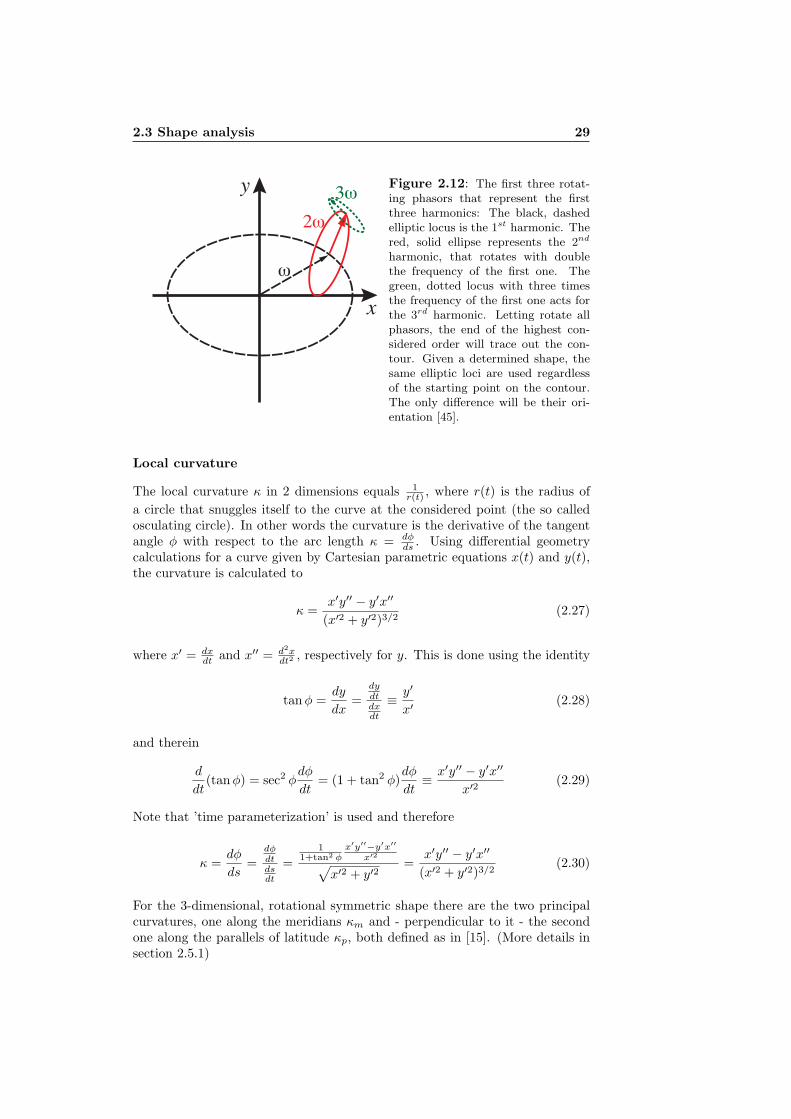
appropriate high order. Amplitudes much smaller than one should have no ef-fect to the pixelated shape. Also frequencies with a wavelength smaller thana pixel should definitely not be considered. As we implicitly assume some de-gree of smoothness for the nuclear membrane, the truncation can be done evenearlier (at lower frequencies). A way of thinking about the different harmon-ics of the truncated FS is similar to Ptolemy’s epicycles (mentioned in section2.1.4). As Kuhl and Giardina [27] already showed, the points (x, y) all haveelliptic loci. So the truncated FS can be seen as the additive accumulation ofrotating phasors, each in proper phase relationship. Each rotating phasor hasits origin on the elliptic locus of the previous one and rotates k times fasterthan the first harmonic (k being its harmonic number). The resulting shapethen is drawn by the end of the phasor of highest respected order. A differentstarting point on the contour does not change the elliptic loci but the phasorswill take a different orientation [45]. Figure 2.12 shows a sketch of the situation.How the different elliptic loci play together to produce the resulting particularshape is visualized at http://lmb.informatik.uni-freiburg.de/lectures/mustererkennung/WS0405/FourierDemo/fourdem.html and choosing a differ-ent number of harmonics clearly shows what the truncation of the FS causes.
2.3.2 Calculating the 2-dimensional properties
Calculation of the properties is an important point, because it allows to drawconclusions about more general features of a particular shape and they arethe basis for more advanced calculations. Given a set of coefficients the localcurvature, the area and the contour length are easily calculated as they dependonly on the first and second derivatives as well as on the x and y values itself.
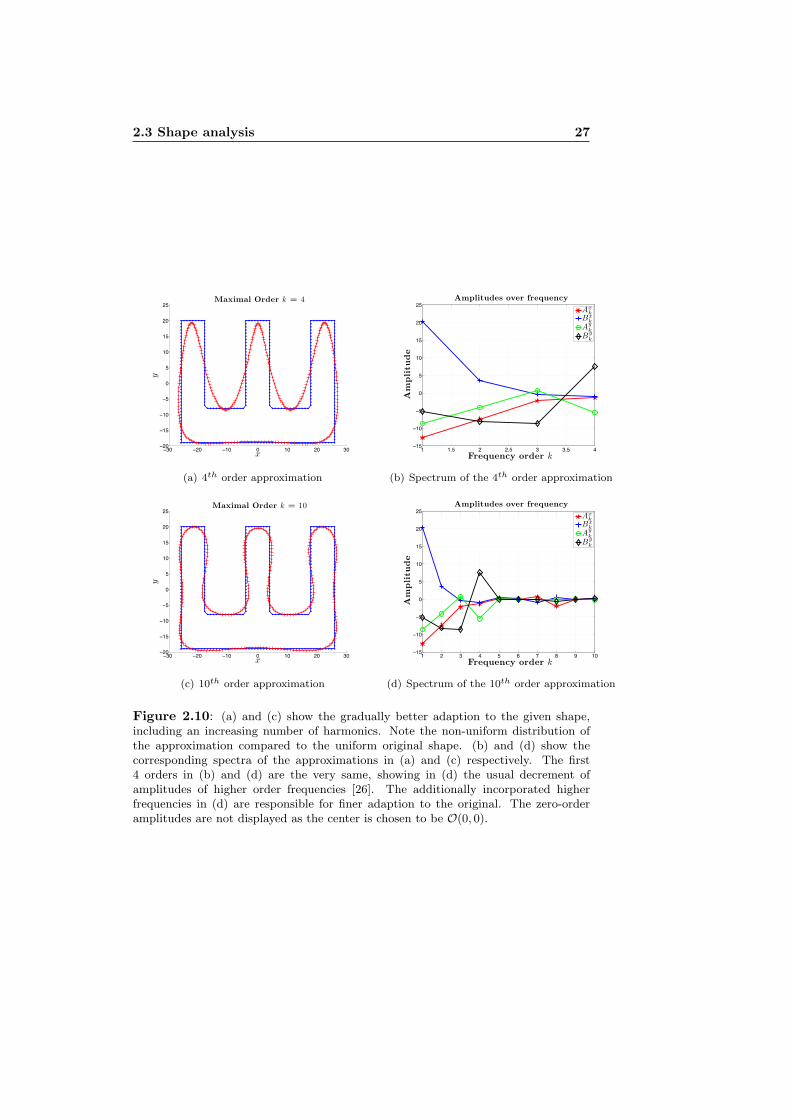
2.3 Shape analysis 27
!30 !20 !10 0 10 20 30!20
!15
!10
!5
0
5
10
15
20
25
x
y
Maximal Order k = 4
(a) 4th order approximation
1 1.5 2 2.5 3 3.5 4!15
!10
!5
0
5
10
15
20
25
Frequency order k
Am
plitu
de
Amplitudes over frequency
Axk
Bxk
Ayk
Byk
(b) Spectrum of the 4th order approximation
!30 !20 !10 0 10 20 30!20
!15
!10
!5
0
5
10
15
20
25
x
y
Maximal Order k = 10
(c) 10th order approximation
1 2 3 4 5 6 7 8 9 10!15
!10
!5
0
5
10
15
20
25
Frequency order k
Am
plitu
de
Amplitudes over frequency
Axk
Bxk
Ayk
Byk
(d) Spectrum of the 10th order approximation
Figure 2.10: (a) and (c) show the gradually better adaption to the given shape,including an increasing number of harmonics. Note the non-uniform distribution ofthe approximation compared to the uniform original shape. (b) and (d) show thecorresponding spectra of the approximations in (a) and (c) respectively. The first4 orders in (b) and (d) are the very same, showing in (d) the usual decrement ofamplitudes of higher order frequencies [26]. The additionally incorporated higherfrequencies in (d) are responsible for finer adaption to the original. The zero-orderamplitudes are not displayed as the center is chosen to be O(0, 0).

28 Methods
0 1 2 3 4 5 6 7!30
!20
!10
0
10
20
30
40
50
60
t
x,
y
Original and recalculated coordinates kmax = 4
recalculated x valuesoriginal x valuesrecalculated y valuesoriginal y values
(a) Comparison of the coordinates (original toapproximated) for the 4th order approximation
0 1 2 3 4 5 6 7!20
!10
0
10
20
30
40
50
60
t
x,
y
Original and recalculated coordinates kmax = 35
recalculated x valuesoriginal x valuesrecalculated y valuesoriginal y values
(b) Comparison of the coordinates for the 35th
order approximation
!30 !20 !10 0 10 20 30!20
!15
!10
!5
0
5
10
15
20
25
x
y
Maximal Order k = 35
(c) 35th order approximation
0 5 10 15 20 25 30 35!15
!10
!5
0
5
10
15
20
25
Frequency order k
Am
plitu
de
Amplitudes over frequency
Axk
Bxk
Ayk
Byk
(d) Spectrum of the 35th order approximation
Figure 2.11: (a) and (b) illustrate the increasing adaption of details by higherharmonics. The crude main features are already visible by 4th order approximation.Like in Figure 2.9(b), the original and approximated curves are displaced against eachother. (c): The 35th order approximation nearly shows no difference to the originalshape. (d): Obvious decreasing of the amplitudes by increasing k. Here it becomesvisible that frequencies higher than 30 can be neglected, as they only try to matchthe pixel-to-pixel digital structure of the object, wich is probably not an importantfeature of the real object.
2.3 Shape analysis 29
x
y
ω
2ω
3ωFigure 2.12: The first three rotat-ing phasors that represent the firstthree harmonics: The black, dashedelliptic locus is the 1st harmonic. Thered, solid ellipse represents the 2nd
harmonic, that rotates with doublethe frequency of the first one. Thegreen, dotted locus with three timesthe frequency of the first one acts forthe 3rd harmonic. Letting rotate allphasors, the end of the highest con-sidered order will trace out the con-tour. Given a determined shape, thesame elliptic loci are used regardlessof the starting point on the contour.The only difference will be their ori-entation [45].
Local curvature
The local curvature κ in 2 dimensions equals 1r(t) , where r(t) is the radius of
a circle that snuggles itself to the curve at the considered point (the so calledosculating circle). In other words the curvature is the derivative of the tangentangle φ with respect to the arc length κ = dφ
ds . Using differential geometrycalculations for a curve given by Cartesian parametric equations x(t) and y(t),the curvature is calculated to
κ =x′y′′ − y′x′′
(x′2 + y′2)3/2(2.27)
where x′ = dxdt and x′′ = d2x
dt2 , respectively for y. This is done using the identity
tanφ =dy
dx=
dydtdxdt
≡ y′
x′(2.28)
and therein
d
dt(tanφ) = sec2 φ
dφ
dt= (1 + tan2 φ)
dφ
dt≡ x′y′′ − y′x′′
x′2(2.29)
Note that ’time parameterization’ is used and therefore
κ =dφ
ds=
dφdtdsdt
=1
1+tan2 φx′y′′−y′x′′
x′2√x′2 + y′2
=x′y′′ − y′x′′
(x′2 + y′2)3/2(2.30)
For the 3-dimensional, rotational symmetric shape there are the two principalcurvatures, one along the meridians κm and - perpendicular to it - the secondone along the parallels of latitude κp, both defined as in [15]. (More details insection 2.5.1)
30 Methods
Area, perimeter and center of perimeter
Area: For the parametrically specified curve, the area calculates to
A =12
∫ 2π
0
(xy′ − yx′)dt (2.31)
assuming that the parameter t ranges from 0 to 2π. This equation isderived by the help of Green’s theorem or the isoperimetric inequality[19] and therefore we do have a signed area and have to travel around theregion such that it lies on the left of our way to get a positive result. In thespecial case of having only first-harmonic amplitudes, the area becomesthe simple form A = π(Ax1 · B
y1 − Bx1 · A
y1). Here it becomes obvious:
When we put Bx1 = Ay1 = 1 and Ax1 = By1 = 0, the resulting circle will bedrawn clockwise. The enclosed area is on the right side of the way andtherefore is denoted negative. Areas of curves with self-intersections mustbe computed as a sum of absolute values of the areas of their componentsand should be excluded here.
Perimeter: The arc length is defined as the length along a curve (see also2.1.4) and so the perimeter here calculates to
L =∫ 2π
0
√x′2 + y′2dt (2.32)
because it is just the sum of the differential arc length ds =√dx2 + dy2
in infinitesimal steps from the starting point along the curve back to itsorigin (= t = 0...2π). Note that this integral (like any property of a curve )is independent of the parameterization [67] (always assuming that a simpleregular curve is considered and hence excluding self-intersection).
Center of perimeter: As it is calculated as a weighted sum over the way alonga curve, its x-component is
x =
∫ 2π
0x(t)
√x′(t)2 + y′(t)2dt
L(2.33)
where L is the perimeter length calculated in equation (2.32). The ycomponent is calculated correspondingly.
2.3.3 Program testing
To be sure the programed code works properly and calculates the right prop-erties, it is crucial to test the written programs by comparing its results withthe analytic solution of well known shapes. Therefore we compare the area,the perimeter length (see Table 2.2) and the local curvature with the expectedvalues derived by the well known formulas A = πr2 for the area and L = 2πrfor the perimeter length of a circle as well as the local curvature. Let be r = 1for the unit circle, then the local curvature is constant and equals 1 for anypoint on the circle. Two different methods are used for the calculation of theperimeter, one using differential geometry (showed in equation (2.32)), the otherone summing up the polygon parts of adjacent points (Archimedes calculated
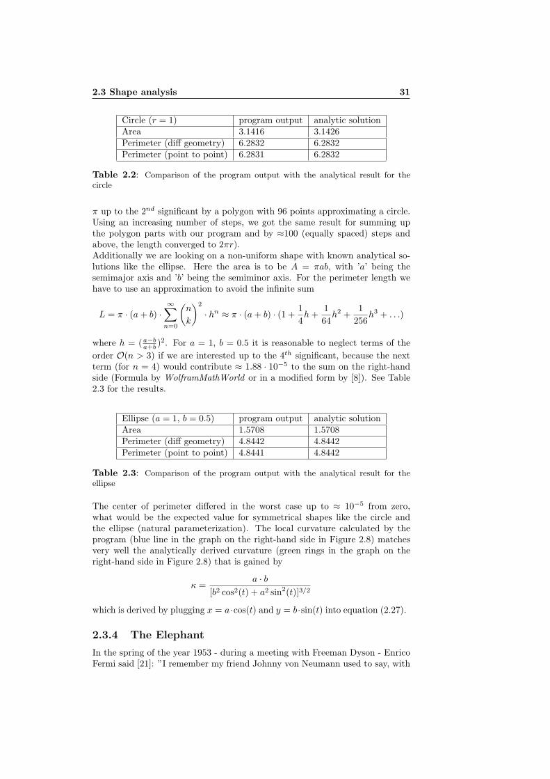
2.3 Shape analysis 31
Circle (r = 1) program output analytic solutionArea 3.1416 3.1426Perimeter (diff geometry) 6.2832 6.2832Perimeter (point to point) 6.2831 6.2832
Table 2.2: Comparison of the program output with the analytical result for thecircle
π up to the 2nd significant by a polygon with 96 points approximating a circle.Using an increasing number of steps, we got the same result for summing upthe polygon parts with our program and by ≈100 (equally spaced) steps andabove, the length converged to 2πr).Additionally we are looking on a non-uniform shape with known analytical so-lutions like the ellipse. Here the area is to be A = πab, with ’a’ being thesemimajor axis and ’b’ being the semiminor axis. For the perimeter length wehave to use an approximation to avoid the infinite sum
L = π · (a+ b) ·∞∑n=0
(n
k
)2
· hn ≈ π · (a+ b) · (1 +14h+
164h2 +
1256
h3 + . . .)
where h = (a−ba+b )2. For a = 1, b = 0.5 it is reasonable to neglect terms of the
order O(n > 3) if we are interested up to the 4th significant, because the nextterm (for n = 4) would contribute ≈ 1.88 · 10−5 to the sum on the right-handside (Formula by WolframMathWorld or in a modified form by [8]). See Table2.3 for the results.
Ellipse (a = 1, b = 0.5) program output analytic solutionArea 1.5708 1.5708Perimeter (diff geometry) 4.8442 4.8442Perimeter (point to point) 4.8441 4.8442
Table 2.3: Comparison of the program output with the analytical result for theellipse
The center of perimeter differed in the worst case up to ≈ 10−5 from zero,what would be the expected value for symmetrical shapes like the circle andthe ellipse (natural parameterization). The local curvature calculated by theprogram (blue line in the graph on the right-hand side in Figure 2.8) matchesvery well the analytically derived curvature (green rings in the graph on theright-hand side in Figure 2.8) that is gained by
κ =a · b
[b2 cos2(t) + a2 sin2(t)]3/2
which is derived by plugging x = a·cos(t) and y = b·sin(t) into equation (2.27).
2.3.4 The Elephant
In the spring of the year 1953 - during a meeting with Freeman Dyson - EnricoFermi said [21]: ”I remember my friend Johnny von Neumann used to say, with

32 Methods
four parameters I can fit an elephant, and with five I can make him wigglehis trunk.” Wei [73] used a least square Fourier sine series to do this, butrequired about 30 terms. With the method described here and the outline of ahand drawn elephant we can fulfill Fermi’s quotation ! Analyzing the picturein Figure 2.13 A) and eliminating amplitudes less than 5.9, we get the ’raw’spectrum. Slightly modifying the remaining amplitudes leads to the spectrumseen in Figure 2.13 B). By applying these coefficients to complex numbers,we have the equivalent of an elephant contour coded in a set of 4 complexparameters. The 5th parameter can be used to let the trunk wiggle (see Figure2.13 C)). More precisely, the real part of the 5th parameter is assigned to a’wiggle parameter’ that sets the x-component where the trunk is supposed tobe attached to the body. Its imaginary part is used to determine the coordinatesof the eye (both x- and y-component). The parameters are compiled in Table2.4 (for details see Legend).
C)
A)
B)
0 2 4 6 8 10−80
−60
−40
−20
0
20
40
60
Frequency order k
Ampl
itude
Axk
Bxk
Ayk
Byk
−100 −50 0 50 100−100
−50
0
50
100
x
y
Figure 2.13:A) This outline of an elephantis used as the pattern that is an-alyzed with the algorithm men-tioned in section 2.3 ’Shape anal-ysis’ to get the coefficients. Asexplained in section 2.3.1 ’De-creasing amplitudes and trunca-tion of the series’ it is reasonableto neglect coefficients that con-tribute very little compared tothe major amplitudes, which willlead to a smoothed shape like inFigure 2.13 C).B) The frequency spectrumof the shapes seen in Figure2.13 C). All high frequenciesfrom the original picture in Fig-ure 2.13 A) are suppressed aswell as all frequencies whose am-plitude is smaller than 5.9. Smallmodifications are then applied tothe remaining ones. The fre-quency order k corresponds tothe summation index in equa-tions (2.10) and (2.11).C) 3 different stages of the wig-gling trunk. 4 parameters areused to determine the shape.The 5th is used for the wigglingand the position of the eye.

2.4 Application to confocal images 33
The resulting shape is quite schematic and cartoon-like, but still recognizableas an elephant.
Parameter real part stands for imaginary part stands forp1 = −60− 30i Ay1 = −60 By1 = −30p2 = 8− 10i By2 = 8 By3 = −10p3 = 12− 14i Ax3 = 12 Ax5 = −14p4 = 50 + 18i Bx1 = 50 Bx2 = 18p5 = 40 + 20i wiggle coefficient = 40 xeye = yeye = 20
Table 2.4: The 5 parameters p1 - p5 that encode the elephant including its wigglingtrunk and what their components stand for. The notation corresponds to that used inequations (2.10) and (2.11), whereas the wiggle coefficient is the x-value of the body+ trunk-attaching-line.
2.4 Application to confocal images
In case of real data images, the contours are mostly not that well defined as isan artificially designed image or even a binary image. The crucial question is tofind the borders of an object in a way that is robust against noise and respectsits properties, such that a best adaption is achieved without falling into pixelartefacts. This is usually done by active contours ([23], [42], [58]) where thegradient and energy functionals are being used. We in our case use the χ2-method and the bending energy to calculate the position of the membrane. Sowe use intrinsic knowledge about the smoothness of the nuclear envelope fordetermining a pareto optimality [10], [13] by computing the L-curve.
2.4.1 From the coefficients to the shape
Having a given set of coefficients, we can mimic a confocal image by translatingthe coefficients to a contour and then convolve it with a PSF and adding Gaus-sian noise. The two latter things just simulate what happens in the microscope.The natural way of thinking to design a curve in a pixelated world is to takethe contour and to cover it with a tiny mesh (several times tinier than the pixelmesh). Every box of this tiny mesh that is intersected by the curve is assignedthe value 1, all the other boxes become 0. This creates a binary image. Thenbinning is applied to regain the original number of pixels. The pixels then havedifferent values according to the length of curve material within the specificpixel. This is to be convolved with the PSF.Another - more analytical - idea is just to convolve the cuve with the PSF. Nu-merically this can be imagined as follows: A symmetric 2-dimensional Gaussiancentered at one particular point of the curve. Then integration over the pixelcontaining this point and also integration over every single pixel in a reasonableneighborhood (≈ 4σ) of the center-pixel is applied and the calculated values areassigned to the corresponding pixels. When this is done for every point of thecurve, we get the desired broadened contour.If we want to create a uniformly distributed intensity, we have to be aware that

34 Methods
the strength S of the line impulse [6] of a function f(x, y) is
S =∣∣∣∣∂f∂~n
∣∣∣∣−1
=1
|grad f |(2.34)
and can be interpreted as the intensity i(t) = 1v(t) defined in section 2.1.4. So
either we have to parameterize by arc length or to multiply by v(t). In the lattercase the points of a curve primarily of uniform intensity but probably differentdistance to its neighbors become values corresponding to the length of its tan-gent vector. Now the convolution with the PSF delivers the broadened contourof uniform intensity. This method will be preferred, as it is computationally lessexpensive than using a finer meshsize (see above) and more accurate becauseno binning is needed.
!1 !0.8 !0.6 !0.4 !0.2 0 0.2 0.4 0.6 0.8 1!1
!0.8
!0.6
!0.4
!0.2
0
0.2
0.4
0.6
0.8
1
x
y
Points of the ellipse
(a) Ellipse (b) Intensity profile
Figure 2.14: (a): The ellipse represented here is not of uniform intensity, but twiceas intense at y = 0 (semimajor axis) as it is at x = 0 (semiminor axis). Every singlepoint however is of the same intensity as all the others. (b): After multiplying theintensity of every point by v(t) and convolving the result with a PSF, the displayedintensity profile is obtained. The intensity is visualized in z-direction. Now the ellipseis of uniform intensity.
As an example consider the ellipse with semimajor axis a = 1 and semiminoraxis b = 0.5 in Figure 2.14(a). The elliptical line impulse [6] and therefore theintensity is twice as great at the ends of the major axis as it is at the end ofthe minor axis (and equally: Neighboring points are twice as dense). Secondarythis reflects the fact that the radial beam coates the same area in a time interval∆t (this is proven using Heron’s formula [8] to calculate the area) and the onlydifference to Keplers third law is that the beam originates in the center insteadof originating in one focus of the ellipse. By multiplying every point (that allhave the same intensity) by v(t) before convolving with the PSF we get theuniformly distributed intensity of Figure 2.14(b). For a better visualization, theintensity is plotted in z-direction.
2.4.2 From the shape to the coefficients
Principally, the way to get the coefficients of a contour is described in section 2.3,but there we assumed a well defined contour. In images like the used confocal
2.4 Application to confocal images 35
images of the S. pombe nucleus, the boundaries are not so well defined. Toget a connection between the shape and the coefficients, the ’artificial’ imageIsynth with known coefficients that we create using the method described in theprevious section is compared with the data image Idata. This is done calculating
χ2 =N∑i=1
[Idata − Isynth(Axk, Bxk , A
yk, B
yk)]2 (2.35)
what is a pixelwise subtraction of the two images, and summing up the squareddifferences. The Idata, Isynth are matrices and the summation index i is goingover all matrix elements. χ2 therefore is a measure for the similarity of the two(grayscale) pictures and called the ’merit function’. Altering the coefficientsleads to a different image and therein a different χ2. The more similar thepictures, the smaller is χ2 and its minimization yields the best-fit-parameters.These hereby found set of coefficients then reproduce the given shape. Mini-mization of χ2 though is equivalent to the maximization of the likelihood of themodel that is optimized, because the probability of the data set is the productof the probabilities of each point [60], so that here it is
P =N∏i=1
e−[Idata−Isynth(Axk,Bxk ,A
yk,B
yk)]2 (2.36)
Maximizing this is equivalent to maximizing its logarithm or equally minimizingthe negative of its logarithm, what leads to equation (2.35).
Data image enhancement
Even though we do have several sections of the nucleus in z-direction, there isno maximum projection applied, because this accumulates also the noise and asdifferent z-stacks have different radii will result in a less accurate determinationof the position of the membrane. The middle section is selected by eye. Tomake it more easy for the algorithm to minimize χ2, the noise in the data imageis suppressed. This is done in two similar steps. First, the 3-by-3 neighborhood,then the 5-by-5 neighborhood of every pixel is examined if there are a specificnumber of pixels below a certain threshold (which is derived by analyzing thehistogram). In the positive case, the accordant pixel is set to zero. As it isvery unlikely to fulfill the conditions near the labeled membrane, there is noloss of information, but most of the noise will be erased. The best results forsmoothing the hereby acquired picture were obtained by using a Gaussian filter.The smoothing makes it easier for the minimization routine (see next section)to find the minimum. Note that the smoothing does not change the center ofthe pattern, it just smears the intensity.
Downhill-simplex- and interior-reflective Newton- method
The problem that we have to solve is to find the minimum of a multivariablefunction, so that we have an unconstrained nonlinear optimization. In MATLAB®
the best two functions to perform minx
f(x) are fminsearch and fminunc. The
first uses the simplex search method of Lagarias et al. [46] and is a direct searchmethod that does not use gradients. It just oozes downhill in the parameter

36 Methods
space until it encounters a minimum (at least a local one). The second is basedon the interior-reflective Newton method described in [11] and either needs agradient provided or locally calculates the gradient. In both methods and evengenerally in optimization problems, the main difficulty is not to fall into a localminimum, when searching for a global one. Starting the algorithm already closeto the global minimum by providing an appropriate set of initial parameters isvery helpful (see next section).No matter which method is used, simply using equation (2.35) and trying tominimize χ2 will rarely lead to success in our case. To be able to compare thetwo images we have to ’normalize’ or scale one of them. This must be done byno other method than calculating a scaling factor γ that minimizes the norm ofthe vector ~sγ = ~d (and therefore its length), so that
γ = min
√√√√ N∑
i=1
(siγ − di)2
(2.37)
where di are the pixel-intensities of Idata, si the pixel-intensities of Isynth andN the overall number of pixels in the images. In other words, γ is the solutionto the system of equations ~sγ = ~d in the least squares sense. Equation (2.35)then has to be modified to
χ2 =N∑i=1
[Idata − γ · Isynth(Axk, Bxk , A
yk, B
yk)]2 (2.38)
A good starting guess
To guarantee a successful result, the initial guess should be very close to thesought contour or at least not too far away. This is best done automatically.The method should provide the initial set of coefficients for a confocal imageof the nucleus in any particular stage during the division. Images obtained bythe procedure explained in section ’Data image enhancement’ (see above) areconsidered. Depending on the quality two different methods were used. Theeasier one is thresholding, neglecting small objects and analyzing the resultingbinary image following section 2.3. The initial contour then is very likely tothe outer edge of the shape in the image. The other one rotates the imagehorizontally (if necessary), calculates the center of the structure, divides theimage at the calculated x-centroid into two pictures (left and right) and againcalculates the center of the structure in the two pictures individually. Thetwo parts are treated likewise and so the following steps are explained onlyfor one part. The centroid becomes the origin O(0, 0) of a jet that scans theimage radial-like to get an intensity profile. A Gaussian profile is fitted to everysingle intensity profile and its center is stored as ~r(Θ). The polar notationis transformed to cartesian coordinates (x,y) and then put together with thecorresponding (x,y) of the other part. The combined (x,y) now represent aclosed contour that lies in the middle of the broad fluorescent structure seen inthe image. These x and y arrays are plugged in the matrix equation (2.26) toget the desired initial coefficients. This is computationally not expensive andthe preferred method. In case of the interior of the shape not clearly belongingto the background (and O(0, 0) therefore not close to zero intensity), the firstmethod is used.

2.4 Application to confocal images 37
Program testing
To assure that - in principle - the algorithm works, an artificially created imageis used as a Idata. Hence, we know exactly all the amplitudes of the coefficientsand can compare them to the ones delivered by the minimization process. Theinitial guess for the coefficients is chosen to be quite far away from the objectiveones. Figure 2.15 shows the iterative process of minimizing χ2 and therein theconvergence of the initial coefficients to their target (which is an ellipse, as allobjective coefficients except Bx1 and Ay1 are chosen to be zero). The first threeharmonics are used, so the minimization is done in a 12 dimensional parameterspace. To estimate how far away the initial guess can be from the objective
50 100 150 200 250 300 350 400 4500
10
20
30
40
50Initial: B1
x = 40 and A1y = 30; Objective: B1
x = 30 and A1y = 20
# of iterations
!2
0 50 100 150 200 250 300 350 400 450 5000
10
20
30
40
# of iteratonsampl
itude
s of
the
coef
ficie
nts
A0x
A1x
A2x
B0x
B1x
B2x
A0y
A1y
Figure 2.15: χ2 (top) and the corresponding amplitudes (bottom) of the used co-efficients are plotted over the iterations of the minimization procedure. An artificialimage (of an ellipse with semiaxes Bx
1 = 30 and Ay1 = 20) is used as the data image.
The initial guess for the semiaxes (Bx1 = 40 and Ay
1 = 30) converges towards the ob-jective values. The three first harmonics are used but only 8 of the used 12 coefficientsare displayed in the legend, as most of them do not depart much from zero.
set of coefficients, an exemplary real data image (nearly circle-shaped) is takenand different combinations of initial parameters are fed to the minimizationalgorithm. It turned out that for the real data it is highly crucial to have agood initial set, as the energy landscape is more jagged.

38 Methods
2.4.3 Bending energy and the L-curve
In addition to the visual information that we get out of the image, we do haveextra knowledge about the nuclear membrane. It is assumed not to be toowrinkled, instead it is supposed to be quite smooth. In general, any bending of amembrane away form its preferred state requires energy, so that the membrane’sresistance to bending stabilizes its shape [38]. Similar to the elastic energy ofthe surface in [15], the bending energy becomes
Eb = kb
∫ 2π
0
(κ− C0)2dt (2.39)
where kb is the elastic modulus, κ the local curvature calculated in equation(2.27) and C0 the spontaneous curvature [37] (the curvature in the natural,stress-free state of the contour). Therewith enters the area difference elasticity(ADE) model, that is connected to the spontaneous curvature model [20], be-cause the effective spontaneous curvature (or equivalently an effective relaxedarea difference) do not enter independently into the model [53]. The Gaussiancurvature and the global curvature are not included due to the fact that they areconstant for the integral over the closed 2-dimensional contour (Gauss-Bonnettheorem and ’turning tangent’ [19]). In accordance to [14] the spontaneous cur-vature can be considered zero, so that we can finally denote the normalizedbending energy as
Eb =1
2π
∫ 2π
0
κ2dt (2.40)
This can be used as a regularization term in our problem of χ2 minimization(originally an ill-posed problem). The energy functional that has to be mini-mized now is
G(Idata, Axk, B
xk , A
yk, B
yk) = χ2(Idata, A
xk, B
xk , A
yk, B
yk)
+ λ · Eb(Axk, Bxk , Ayk, B
yk) (2.41)
where λ is the regularization parameter, that balances between the external im-age energy (χ2) and the internal contour energy (Eb). In other words it weightsthe importance of smoothing the whole contour and the accuracy of fitting tothe data image. The bigger λ, the smoother the shape and equivalently thelower Eb. The other way round: The smaller λ (and therein less important Eb),the closer the fit to the data and the more wrinkled the contour.The same arguments as in [43] (computational affordable and incorporation ofprior knowledge) account for using the L-curve method [36] to determine λ in-stead of minimizing the cross-validation or minimizing a Bayesian informationcriterion. Therefore the functional G is minimized every time, while λ is varied.Having reached the minimum for a particular λ, the logarithm of the achieved Ebis plotted over the logarithm of the corresponding χ2 and the point is assignedthe actual λ. The resulting ’curve’ is L-shaped and is a trade-off between twoquantities that both should be controlled. The λ-values in the corner of the Lcorrespond to a transition between the two legs and the graphically determinedoptimal λ reflects the pareto optimality. Vogel [72] pointed out that the com-puted optimal λ is not the optimal parameter λopt, when the dimension of the

2.4 Application to confocal images 39
system increases significantly. This limitation to the L-curve is not met here,but in general the method tends to over-regularize and so to over-smoothing[35]. Additional attention has to be paid to the corner, when the regularizationparameter is discrete (as in our case), because then the L-curve tends to clus-ter in a neighborhood of the corner [62]. Taking the image (processed by the
!"# !"$!"!%
!"!&
'()*!&+
'()*
, -+
./0 2!34560
" # 7 !"! ! !"#8#
" # 7 !"$
" # 7 !"$8#
" # 7 !"
9
" # 7 !"98#" # 7 !":
" # 7 !":8#
" # 7 !";
Figure 2.16: A double logarithmic plot of Eb against χ2. Every star is the resultof minimizing G in equation (2.41) having a different, fixed λ value. The bottom, leftimage in Figure 1.4 is used as raw data image. The corner of the L-curve (λ = 107) isthe optimal λ that respects both, the smoothness of the fit as well as closeness to thedata. It is marked in red and displayed vertically. The ’horizontal’ branch of the ’L’stands for the overregulated system, the vertical branch for the underregularized.
method described in section ’Data image enhancement’) of the peanut-shapednucleus and variating λ in equation (2.41) from 101 to 109 before minimizing G,we get the L-curve seen in Figure 2.16. The optimal λ is chosen to be λ = 107
(marked in red and written vertically), what expresses best the corner of the ’L’.The first point belonging to different λ values reflects the fact that the bendingenergy is weighted too lightly to play any role in the minimization of the energyfunctional G and the problem is not regularized. To recognize the influenceof λ concerning the calculated shape see Figure 2.17. The resulting shape isoverlaid with the analyzed image. If λ is too small (top), the contour sticks toomuch to to the data, giving it an uneven appearance. Having a λ that is toohigh (bottom) results in a very smooth contour, but does not reflect the givendata any more. Every additional curvature (more bending energy) would betoo expensive for the energy functional. A further increase of λ would enforcea more and more circle-like contour. The chosen λ = 107 (middle) does both,smoothing the curve (and therefore respecting the additional knowledge about

40 Methods
! = 101 ! 105.5
! = 107
! = 109
Figure 2.17: Overlay of thedata image (after removing back-ground and smoothing in the rawdata image, see section ’Data im-age enhancement’) and the re-sulting contour by minimizingthe functional G in equation(2.41) for different, fixed λ val-ues. For a wide range of small λvalues there is no difference, be-cause Eb is weighted too smalland hence is not important com-pared to χ2. The problem is stillunregulated and the contour fitsbest to the data (top), but hasirregularities respective its cur-vature. λ = 109 (bottom) pro-duces an over-smoothed shape,because of over-regularization.The bending energy has becomevery important and outweighsthe closeness to the data. Onlythe best-fit parameter λ = 107
(middle) balances the two ne-cessities and we have a smoothcurve, that also reflects the data.The additional knowledge aboutthe smoothness of the membraneis incorporated without disre-garding the data.
the membrane) as well as reproducing the given data. This best λ value is thenused to calculate the properties of the nucleus.
2.5 Extension to 3-d
The yeast nucleus is a 3-dimensional structure, so we should not restrict our-selves to 2 dimensions. Considering the space curve ~p(t) in three dimensions weget
~t(t) =d~p(t)dt∣∣∣d~p(t)dt
∣∣∣ =d~p(t)dtdsdt
as already showed in equation (2.18) and the curvature calculates to [32]
κ =∣∣∣∣ d~tds∣∣∣∣ =
∣∣∣d~pdt × d2~pdt2
∣∣∣∣∣∣d~pdt ∣∣∣3 =|~p ′ × ~p ′′||~p ′|3
(2.42)

2.5 Extension to 3-d 41
where
~p(t)′′ = ~t(t)′ =d
dt~t(t) = κ
ds
dt~n(t) (2.43)
and ~n being the unit normal vector with
~n =d~tds∣∣∣ d~tds ∣∣∣ =
d~tdt∣∣∣d~tdt ∣∣∣ =
1κ
d~t
ds(2.44)
so that we have very important derivative relations (that are related to theFrenet formulas)
d~p(s)ds
= ~t(s) (2.45)
d2~p(s)ds2
= κ~n(s) (2.46)
d3~p(s)ds3
= κ~n(s) + κ[τ~b(s)− κ~t(s)
](2.47)
det(d~p(s)ds
d2~p(s)ds2
d3~p(s)ds3
)= κ2τ (2.48)
where ~b(s) is the binormal vector and τ the torsion [12]. A curve however isnot enough, as we have to deal with surfaces and volumes. A surface can bedescribed by its principal curvatures. The Gaussian curvature
K = κmκp =1
RmRp(2.49)
is the product of the two principal curvatures (that is identical to the inverseproduct of the principal radii of curvature) and is an intrinsic feature. TheGauss-Bonnet theorem [19] for a compact, boundaryless 2-dimensional surface∮
surface
KdA = 2πχ (2.50)
displays the fact that the integral of the Gaussian curvature over the surfaceis topologically invariant and means that all surfaces with the same numberof handles or holes have the same integral Gaussian curvature. This is aninteresting fact, because χ - the Euler-Poincare characteristic [40] - does notat all depend on differential geometry, but puts a constraint on the curvature(what is a local property). Imagine a closed surface without holes like the sphere(χ = 2). It can be arbitrarily deformed (for example to the dumbbell shape ofthe nucleus where also χ = 2) but the total curvature is maintained, becauseimplying an additional region of negative curvature will always be compensatedby a corresponding positive integral curvature in other regions. This fact is usedto assure the correctness of our computations. The mean curvature calculatesto
H =12
(κm + κp) =12
(1Rm
+1Rp
) =12
(Rm +Rp)K (2.51)

42 Methods
and is used in the energy calculation of a membrane. The so called Helfrich-Canham free energy [14] is defined as
FH−C =∮surface
[kb2
(2H)2 − kb2HC0
]dA (2.52)
where kb is the bending rigidity of the membrane and C0 the spontaneous curva-ture (that characterizes the asymmetry of the membrane due to different innerand outer medium or lipid composition on the two sides). The model assumesthe inner and outer NE as axisymmetric with a fixed interbilayer distance, con-nected via the NPCs. Minimizing this free energy, whereas respecting system-specific constraints and boundary conditions, we come to the equilibrium stateof the membrane. The surface area A and the enclosed volume V (that areboth calculated in the next section) can be considered constant analyzing oneparticular image of the nucleus during its division. They are denoted A0 andV0 respectively. These constraints can be implemented into equation (2.52) bythe terms σA− pV , where σ and p are the Lagrange multipliers [18]. The freeenergy therein becomes
FH−C =∮surface
[kb2
(2H)2 − kb2HC0 + σ
]dA− pV (2.53)
The Lagrange multipliers have to be chosen in a way that the correspondingconstraints (A = A0, V = V0) are fulfilled and their physical meaning willbecome the surface tension (σ) and the pressure difference between inside andoutside the nucleus (p).
2.5.1 Calculating the 3-dimensional properties
For visualization of the 3-D appearance, we processed data acquired by the ZeissUV (see section 1.3.3), using Imaris® (Bitplane AG) - software (threshold level20/200, Gaussian filter width 0,2 µm). Figure 2.18 shows the nucleus duringa stage similar to the one examined in section 2.4.3. To describe a figure in
Figure 2.18: 3-d recon-struction of the nucleus dur-ing telophase, using data ac-quired by the Zeiss UV. Despitesmoothing, the surface is stillcorrugated due to the irregularlabeling of the membrane. Us-ing the (aligned) rotating curvecalculated by the L-curve (seesection 2.4.3), we will get rid ofthese surface irregularities.
3 dimensions in terms of an expansion of basis functions we could use sphericalharmonics (that are the 3-D equivalent to the FS) as Khairy [43] in his workabout red blood cells or Brechbuhler [7] describing closed surfaces. We then
2.5 Extension to 3-d 43
could use for x, y and z the alike expansion separately
x(Θ, φ) =∞∑l=0
l∑k=−l
Cxkl Y
kl (Θ, φ) (2.54)
where Θ = 0...π and φ = 0...2π. The Cxkl are the coefficients and Y kl (Θ, φ) thespherical harmonics [25].But we take advantage of the rotational symmetry of the nucleus and assumethe x-axis to be the rotational axis. Adapting Helfrich’s notation [15] for shapesof rotational symmetry to our notation, we have: κm is along the meridians andκp along the parallels of latitude. But note that the surface normal generally liesnot in the plane containing these parallels and the radius of curvature thereforeis not the radius of these circles. In fact Rp is the distance between the twopoints where the surface normal penetrates the surface and where it intersectsthe x-axis. Helfrich’s notation is changed from z(x) to y(x) and the axis ofrevolution is flipped from vertical to horizontal, which is equivalent to flippingx ↔ y. As the angle ψ still denotes the angle between the axis of revolution(here the x-axis) and the surface normal, we get κp = sinψ
y . In our case ofhaving the parameterized curve (x(t), y(t)) defined above, this leads to
κp =|x′|
|y|√x′2 + y′2
(2.55)
Coevally this is the 2nd principal curvature. The 1st principal curvature (κm)is the curvature calculated in equation (2.27) on page 29. For accuracy weshould mention that the usual calculation in the above equation is done by −x′instead of |x′| and equation (2.27) additionally is multiplied by sgn(y). Thiswould become important dealing with overhangs. However, we can keep thenotation for convenience in calculating the Gaussian and mean curvature usingthe whole, closed contour instead of only [0, T2 ] (see section 2.5.2).
Volume of revolution
The rotational symmetry suggests to use cylindrical coordinates and we there-fore calculate the volume of a rotational symmetric corpus by
V =∫ R
0
∫ 2π
0
∫ L
−Lrdrdθdl =
∫ L
−LπR2dl
This is the intuitive way of summing up infinitesimal thin disks of radius R(l).In our case this leads to
V = π
∫ x1
x0
[y(x)]2dx (2.56)
as used in [8], where we are bound to have a unique function, so that we mustexclude overhangs in x-direction. But as one can see in the exemplary imagesof Figure 1.1 this condition is not violated. The integration goes from theminimum x-value to the maximum x-value. (If one would integrate vice versa,the absolute value would have to be taken because of the negative dx.) Using
44 Methods
the parameterization this formula becomes
V = π
∫ t1
t0
[y(t)]2x(t)′dt (2.57)
where t0 and t1 correspond to x0 = x(t0) and x1 = x(t1). Now, even overhangscan occur, because x′ is of the opposite sign in the overhang-region and hencesubtracts the volume between the overhang and the x-axis. Another possibilityto calculate the volume is using the formula provided in [15], what leads to
dV = πy3κp(1− y2κ2p)−1/2dx (2.58)
Surface of revolution
The area element of a curve rotated around the x-axis is dA = 2πyds (ds is thedifferential arc length calculated in section 2.3.2 ’Area, perimeter and center ofperimeter’). Replacing ds and using the integral over the parameter t gives
A = 2π∫ t1
t0
y(t)√x(t)′ 2 + y(t)′ 2dt (2.59)
for the entire surface area. Here there is also no constraint to avoid overhangsand t ranges from 0 to 2π (as stated calculating the perimeter in section 2.3.2),what automatically reflects the fact that we have a closed contour.Following [15] there is the alternative calculation
dA = 2πx(1− x2κ2p)−1/2dx (2.60)
2.5.2 Program testing
Like for the 2-D properties, it is equally important to test the programmed codefor the 3-D ones. First, take a circle with radius r = 2 (Ax1 = By1 = 2) andcompare the output with the result of the formulas S = 4πr2 for the surface ofa sphere and V = 4
3πr3 for its volume.
Plugging the principal curvatures from equation (2.27) and (2.55) into equation(2.49) for the Gaussian curvature and into (2.51) for the mean curvature leadsto
K =y′′x′|x′| − y′|x′|x′′
|y|(x′2 + y′2)2(2.61)
H =12|y|(y′′x′ − y′x′′) + |x′|(x′2 + y′2)
|y|(x′2 + y′2)3/2(2.62)
These formulas uses the program for its calculations and their results are there-fore compared to the analytic solutions. Table 2.5 shows the results for thesphere. The ellipsoid with semi-axes a, b and c is a good non-uniform curvedobject to test the program. As rotational symmetry is assumed, the ellipsoidbecomes a spheroid and b = c. A spheroid’s volume is V = 4/3πab2. For its sur-face the calculation differs between a prolate (a > b) and an oblate (a < b) one.

2.5 Extension to 3-d 45
Sphere (r = 2) program output analytic solutionSurface 50.2655 4π(2)2 ≈ 50.2655Volume 33.5103 4
3π(2)3 ≈ 33.5103Gaussian curvature 0.25 0.25Mean curvature 0.5 0.5
Table 2.5: Comparison of the program output with the analytical result for thesphere. Surface, volume, Gaussian and Mean curvature are compared and approve thecorrectness of the calculations.
Using the notation from WolframMathWorld, the surface of a prolate spheroidis
S = 2πb2 +2πabe
arcsin(e) (2.63)
where e =√
a2−b2a2 denotes the ellipticity and (a > b). In the case of an oblate
spheroid, the formula becomes
S = 2πb2 +2πa2
eln(
1 + e
1− e
)(2.64)
In this case the ellipticity e =√
b2−a2
b2 and naturally (a < b). The resultstherefor can be seen in Table 2.6. The Gaussian and mean curvature for a non-uniform curved object like the spheroid are obviously different from point topoint and are compared in the graphs seen in Figure 2.19. It is sufficient to usea 2-dimensional plot, because κp remains constant for every fixed parameter t(due to the rotational symmetry). The continuously plotted curves refer to thecurvatures calculated by the program, the circles and diamonds are derived byan analytic calculation using the formulas
K =4a2
[b2 + a2 + (b2 − a2) cos(2t)]2(2.65)
for the Gaussian curvature of a spheroid and
H =a[3b2 + a2 + (b2 − a2) cos(2t)]√
2 · b · [b2 + a2 + (b2 − a2) cos(2t)]3/2(2.66)
for its mean curvature. The same notation is used as before (a, b: semi-axes; t:parameter).
2.5.3 Alignment
Before we can rotate the contour however, we have to assure that the long axisis aligned with the x-axis. Therefor we can calculate the covariance matrix
V = cov(X,X) cov(X,Y )
cov(X,Y ) cov(Y, Y )
(2.67)
where cov(X,Y ) =∑Ni=1
(xi−x)(yi−y)N , and then search for the eigenvector with
the larger eigenvalue. This vector is along the long axis of the contour, which
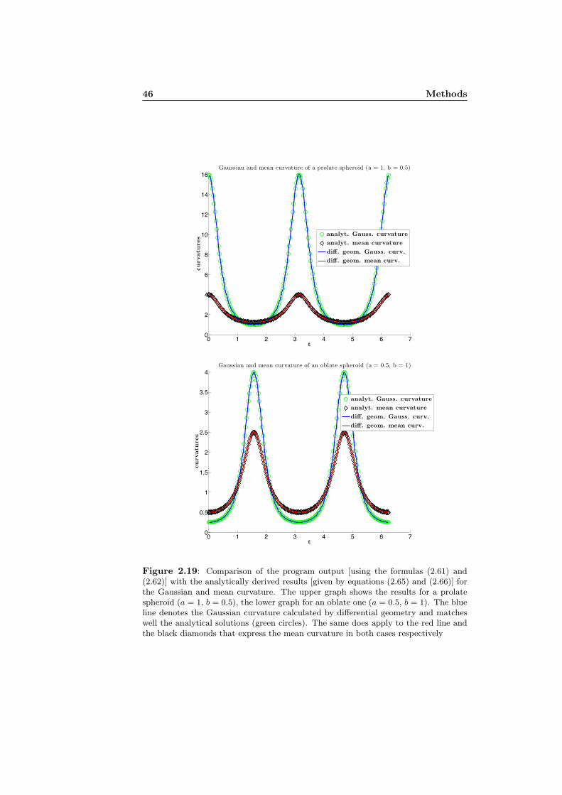
46 Methods
0 1 2 3 4 5 6 70
2
4
6
8
10
12
14
16
t
curv
ature
s
Gaussian and mean curvature of a prolate spheroid (a = 1, b = 0.5)
analyt. Gauss. curvatureanalyt. mean curvaturedi!. geom. Gauss. curv.di!. geom. mean curv.
0 1 2 3 4 5 6 70
0.5
1
1.5
2
2.5
3
3.5
4
t
curv
ature
s
Gaussian and mean curvature of an oblate spheroid (a = 0.5, b = 1)
analyt. Gauss. curvatureanalyt. mean curvaturedi!. geom. Gauss. curv.di!. geom. mean curv.
Figure 2.19: Comparison of the program output [using the formulas (2.61) and(2.62)] with the analytically derived results [given by equations (2.65) and (2.66)] forthe Gaussian and mean curvature. The upper graph shows the results for a prolatespheroid (a = 1, b = 0.5), the lower graph for an oblate one (a = 0.5, b = 1). The blueline denotes the Gaussian curvature calculated by differential geometry and matcheswell the analytical solutions (green circles). The same does apply to the red line andthe black diamonds that express the mean curvature in both cases respectively

2.5 Extension to 3-d 47
Spheroid (a = 1, b = 0.5)→ prolate program output analytic solutionSurface 5.3696 5.3696Volume 1.0472 4
3π · 1 · (0.5)2 ≈ 1.0472Spheroid (a = 0.5, b = 1)→ oblate program output analytic solutionSurface 8.6719 8.6719Volume 2.0944 4
3π · 0.5 · (1)2 ≈ 2.0944
Table 2.6: Comparison of the program output with the analytical result for a prolateand an oblate spheroid. In both cases the surface as well as the volume are comparedand the results coincide.
has to be rotated to the x-axis. Or we can follow Khairy [43] and therewithBrechbuhler [7] in finding the translational and rotational invariant form. Theobject is rotated to canonical positions in parameter space and in object space.The set of parametric equations for a general ellipse is written
~p(t) = x(t)
y(t)
= Ax1 Bx1
Ay1 By1
· sin(t)cos(t)
= Ax1 sin(t) +Bx1 cos(t)
Ay1 sin(t) +By1 cos(t)
(2.68)
where the matrix of coefficients
M = Ax1 Bx1
Ay1 By1
(2.69)
determines the length of the semi-axes and the orientation of the ellipse in thecoordinate system. The matrix H = MT ·M has to be rotated into its principalaxis system by transforming it into a diagonal matrix. More precisely it is
H = a c
c b
= [Ax1 ]2 + [Ay1]2 Ax1B
x1 +Ay1B
y1
Bx1Ax1 +By1A
y1 [Bx1 ]2 + [By1 ]2
= MT ·M (2.70)
what yields
a = [Ax1 ]2 + [Ay1]2 b = [Bx1 ]2 + [By1 ]2 c = Ax1Bx1 +Ay1B
y1 (2.71)
That is the direct connection to the general ellipse equation
ax2 + by2 + 2cxy = 0 (2.72)
where indeed the equations (2.71) hold and c = 0 then gives the canonical formwith the length of the semi-axes 1√
aand 1√
b.


3
Conclusions and Outlook
So far the described methods work and we take advantage of incorporatingadditional knowledge about the assumed closeness and smoothness of the mem-brane into our calculations. The expected behavior plotting the area and thebending energy over time would be some remarkable change coincident with anadditional force acting on the nucleus. The additional force could be integratedinto equation (2.53) by an additional Lagrange multiplier [14], respecting theadditional constraint on the length along the x-axis. The new energy functionalto minimize then would be
FH−C =∮surface
[kb2
(2H)2 − kb2HC0 + σ
]dA− pV − fL (3.1)
where f is the additional force (and simultaneously the new Lagrange multiplier)and L the overall length of the nucleus. This force is most likely exerted by themitotic spindle, as explained in section 1.2.1 and it is shown [47] that this forceonly can be assigned to a broad area of the membrane by a spindle properlyanchored at the SPB. Otherwise the membrane tries to minimize surface area atthe expense of high curvature regions, yielding to tether formation. The samereason should hold for the formation of the tube in the dumbbell-shape. Thecurious thing about the visibility of the tube connecting the two bulbs in thedumbbell-shape stage is (see Figure 1.4 on page 7) that there is often no signal,although it should be ≈ 1
4 of the intensity of the bulb region considering the baremembrane material (see also section 1.2.2). Hereby a tube diameter of ≈100 nm(enough for 6-8 MT’s) is assumed and the fact that the tube is not always in thefocus plane of the LSCM. But even without any signal, the algorithm completesthe dumbbell, showing its full supremacy compared to classical segmentationmethods. The delicate part here is to avoid self-intersection, which can easilyoccur dealing with shapes similar to Figure 2.5(d). The pareto-optimum includ-ing the bending energy delightfully avoids sharp edges and cusps by smoothingthe surface, but there is no elegant way to inhibit self-intersection. At the costof computationally expensive calculations however, we can impede it. The oc-currence of turnings at the transition from the bulb to the tube will provokeovershootings, even using a huge amount of coefficients. They can indeed besuppressed using Lanczos sigma factor, as explained in section 2.1.1.In summary we will calculate the surface area and the enclosed volume of theobserved nuclei and use them as constraints on the free energy function mini-

50 Conclusions and Outlook
mization like outlined before. After minimization we expect to get shapes verysimilar to the observed ones until a certain time during morphogenesis (for ex-ample after the peanut-like shape) where the observed shape differs from the’natural’ minimal energy shape. This is the time where new constraints mustoccur. An experiment to prove the idea of the spindle being mainly responsiblewould be to cut the spindle of a dumbbell-shaped nucleus by laser ablation andto see if the nucleus shrinks back to an earlier stage. The central assumption ofthe model is that the nucleus assumes a shape that minimizes its overall mem-brane energy subject to the appropriate constraints, first without the additionallength constraint, then including it.Regarding the nuclear envelope like an artificial vesicle may be too simple as thenuclear membrane embeds other proteins like the NPC or consist of differenttypes of lipids and therefore may be spatially inhomogeneous. But taking twodifferent molecular species, it has been shown that it simply rescales the elasticparameters of the membrane [14].Additionally to the very useful investigation of the fission yeast nucleus, there isa wide field of possible applications for our method describing shapes. It couldbe used for an automated pollen recognition like in [63] where fluorescence mi-croscopy is used to image the pollen. The description in terms of coefficientsshould be sensitive enough to distinguish between them. The registration ofplant leaves using shape analysis [51] where Kuhl and Giardina’s method [45]was successfully applied is another example, or thinking of C. elegans embryoswith a non-uniformly distributed signal, our method could also be very helpful.It is a very promising project, where further investigation is worthwhile.The presented work makes it possible to use equation (3.1) and subsequentlyis a tool to derive forces based on images ! When we will have determined theforces, we can prove or reject the idea of the mitotic spindle applying the mainforce that drives the spatial division of the forming daughter nuclei or ratherwhere other or additional mechanisms have to participate. The answer to thisquestion will be a big step forward in understanding the cell cycle and a longawaited push giving rise to further investigations. We have developed a newmethod that is particularly suitable for image processing of confocal images,that especially occur in a wide range of life sciences, but is generally applicablefor any pattern recognition in terms of determining shapes.

Appendix A
Protocol
Protocol for 1liter of EMM (Edinburgh Minimal Medium):
3 g C8H5KO4
2.2 g Na2HPO4
5 g NH4Cl20 g Glucose → final concentration: 2%20 ml 50x salt solution1 ml solution A1(minerals)1 ml solution A2a (vitamins)1 ml solution A2b(20 g agar for the plates)
wherein the solutions consist of the following:
A1: 5 g/l boric acid 80.9 mM4 g/l MnSO4 23.7 mM4 g/l ZnSO4.7H2O 13.9 mM2 g/l FeCl2.6H2O 7.40 mM0.4 g/l molybdic acid 2.47 mM1 g/l KI 6.02 mM0.4 g/l CuSO4.5H2O 1.60 mM
A2a: 1 g/l pantothenic acid 4.20 mM10 g/l nicotinic acid 81.2 mM10 g/l inositol 55.5 mM
A2b: 10 mg/l biotin 40.8 µM


Appendix B
List of abbreviations
S phase synthesis phaseG1, 2 phase gap phase 1, 2M phase mitotic phaseMT microtubuleMTOC microtubule-organizing centersSPB spindle pole bodyNE nuclear envelopeKlp kinesin-like proteinsGFP Green fluorescent proteinSOI structure of interestNPC nuclear pore complexLSCM laser scanning confocal microscopePSF point spread functionFWHM full-width-half-maximumNA numerical aperturePMT photomultiplier tubeEMM Edinburgh Minimal MediumFS Fourier seriesMR magnetic resonanceADE area difference elasticity


Bibliography
[1] Gene database. URL http://www.genedb.org/.
[2] Stephen A. Adam. The nuclear pore complex. Genome Biology,2(9):reviews00007.1–00007.6, August 2001.
[3] Bruce Alberts, Dennis Bray, Alexander Johnson, Julian Lewis, Martin Raff,Keith Roberts, and Peter Walter. Essential cell biology. Garland Publish-ing, 1998.
[4] Bruce Alberts, Alexander Johnson, Julian Lewis, Martin Raff, KeithRoberts, and Peter Walter. Molecular biology of the cell. Garland Science,2002.
[5] C. Bauer, V. Herzog, and M.F. Bauer. Improved technique for electronmicroscope visualization of yeast membrane structure. Microsc Microanal,7(6):530–534, 2001.
[6] Ronald N. Bracewell. Fourier analysis and imaging. Kluwer Academic,2003.
[7] Ch. Brechbuhler, G. Gerig, and O. Kubler. Parametrization of closed sur-faces for 3-d shape description. Computer Vision and Image Understanding,61(2):154–170, 1995.
[8] I.N. Bronstein, K.A. Semendjajew, G. Musiol, and H. Muhlig. Taschenbuchder Mathematik. Verlag Harri Deutsch, 2000.
[9] P. B. Canham. The minimum energy of bending as a possible explanationof the biconcave shape of the human red blood cell. Journal of TheoreticalBiology, 26(1):61–81, 1970.
[10] Yair Censor. Pareto optimality in multiobjective problems. Applied Math-ematics and Optimization, 4(1):41–59, 1977.
[11] Thomas F. Coleman and Yuying Li. On the convergence of interior-reflective newton methods for nonlinear minimization subject to bounds.Mathematical Programming, 67(1-3):189–224, 2005.
[12] Harold S. M. Coxeter. Unvergangliche Geometrie. Birkhauser, 1981.
[13] N. O. Da Cunha and E. Polak. Constrained minimization under vector-valued criteria in finite dimensional spaces. Journal of Mathematical Anal-ysis and Applications, 19:103–124, 1967.

56 BIBLIOGRAPHY
[14] I. Derenyi, G. Koster, M. M. van Duijn, A. Czovek, M. Dogterom, andJ. Prost. Membrane nanotubes. Controlled Nanoscale Motion, pages 141–159, 2007.
[15] H.J. Deuling and W. Helfrich. Red blood cell shapes as explained on thebasis of curvature elasticity. Biophys J, 16(8):861–8, 1976.
[16] R Ding, KL McDonald, and JR McIntosh. Three-dimensional reconstruc-tion and analysis of mitotic spindles from the yeast, Schizosaccharomycespombe. J. Cell Biol., 120(1):141–151, 1993.
[17] R Ding, RR West, DM Morphew, BR Oakley, and JR McIntosh. Thespindle pole body of Schizosaccharomyces pombe enters and leaves thenuclear envelope as the cell cycle proceeds. Mol. Biol. Cell, 8(8):1461–1479, 1997.
[18] Bernard Diu, Claudine Guthmann, Danielle Lederer, and Bernard Roulet.Physique statistique. Hermann, 1989.
[19] Manfredo P. do Carmo. Differentialgeometrie von Kurven und Flachen.Vieweg, 1992.
[20] H.-G. Dobereiner, E. Evans, M. Kraus, U. Seifert, and M. Wortis. Mappingvesicle shapes into the phase diagram: A comparison of experiment andtheory. Phys. Rev. E, 55(4):4458–4474, Apr 1997.
[21] F. Dyson. A meeting with enrico fermi. Nature, 427(22):297, January 2004.
[22] Richard Egel. The Molecular Biology of Schizosaccharomyces pombe.Springer-Verlag Berlin, 2004.
[23] H. Eviatar and R. L. Somorjai. A fast, simple active contour algorithm forbiomedical images. Pattern Recogn. Lett., 17(9):969–974, 1996.
[24] Rida T. Farouki and Hwan Pyo Moon. Bipolar and multipolar coordi-nates. In IMA Conference on the Mathematics of Surfaces, pages 348–371.Springer-Verlag, 2000.
[25] Torsten Fließbach. Elektrodynamik - Lehrbuch zur theoretischen Physik,volume 3. Spektrum Akademischer Verlag, 2005.
[26] E. J. Garboczi. Three-dimensional mathematical analysis of particle shapeusing x-ray tomography and spherical harmonics: Application to aggregatesused in concrete. Cement and Concrete Research, 32(10):1621–1638, 2002.
[27] Charles R. Giardina and Frank P. Kuhl. Accuracy of curve approximationby harmonically related vectors with elliptical loci. Computer Graphics andImage Processing, 6(3):277–285, June 1977.
[28] Johan Gielis. A generic geometric transformation that unifies a wide rangeof natural and abstract shapes. Am. J. Bot., 90(3):333–338, 2003.
[29] Yuko Giga-Hama and Hiromichi Kumagai. Foreign Gene Expression in Fis-sion Yeast Schizosaccharomyces pombe. Springer-Verlag Berlin and LandesBioscience Georgetown, 1997.

BIBLIOGRAPHY 57
[30] F Gittes, B Mickey, J Nettleton, and J Howard. Flexural rigidity of micro-tubules and actin filaments measured from thermal fluctuations in shape.J. Cell Biol., 120(4):923–934, 1993.
[31] Alfred Gray. Differentialgeometrie, Klassische Theorie in modernerDarstellung. Spektrum Akademischer Verlag, 1994.
[32] Alfred Gray, Elsa Abbena, and Simon Salamon. Modern Differential Ge-ometry of Curves and Surfaces with Mathematica. Chapman and Hall /CRC Press, 2006.
[33] Walter Greulich. Lexikon der Physik (Band 2). Spektrum AkademischerVerlag, 1999.
[34] IM Hagan. The fission yeast microtubule cytoskeleton. J Cell Sci,111(12):1603–1612, 1998.
[35] P.C. Hansen. The l-curve and its use in the numerical treatment of inverseproblems. In InviteComputational Inverse Problems in Electrocardiology.WIT Press, 2000.
[36] Per Christian Hansen. Rank-deficient and discrete ill-posed problems: nu-merical aspects of linear inversion. Society for Industrial and AppliedMathematics, Philadelphia, PA, USA, 1998.
[37] W Helfrich. Elastic properties of lipid bilayers: theory and possible exper-iments. Z Naturforsch [C], 28(11):693–703, 1973.
[38] R M Hochmuth and R E Waugh. Erythrocyte membrane elasticity andviscosity. Annual Review of Physiology, 49(1):209–219, 1987.
[39] Joe Howard and Anthony A. Hyman. Dynamics and mechanics of themicrotubule plus end. Nature, 422(6933):753–758, 2003.
[40] Stephen Hyde, Sten Andersson, Kare Larsson, Zoltan Blum, Tomas Landh,Sven Lidin, and Barry W. Ninham. The language of shape. Elsevier ScienceB.V., 1997.
[41] Alan Isaacs. A dictionary of physics. Oxford University Press, 2003.
[42] M. Kass, A. Witkin, and D. Terzopoulos. Snakes: Active contour models.International Journal of Computer Vision, 1:321–331, 1988.
[43] Khaled Khairy and Jonathon Howard. Spherical harmonics-based paramet-ric deconvolution of 3d surface images using bending energy minimization.Medical Image Analysis, In Press, Corrected Proof:–, 2007.
[44] Ulrich Kilian and Christine Weber. Lexikon der Physik (Band 4). SpektrumAkademischer Verlag, 2000.
[45] Frank P. Kuhl and Charles R. Giardina. Elliptic fourier features of a closedcontour. Computer Graphics and Image Processing, 18:236–258, 1982.
[46] Jeffrey C. Lagarias, James A. Reeds, Margaret H. Wright, and Paul E.Wright. Convergence properties of the nelder–mead simplex method in lowdimensions. SIAM Journal on Optimization, 9(1):112–147, 1998.

58 BIBLIOGRAPHY
[47] Gerald Lim H. W., Greg Huber, Yoshihiro Torii, Aiko Hirata, JonathanMiller, and Shelley Sazer. Vesicle-like biomechanics governs important as-pects of nuclear geometry in fission yeast. PLoS ONE, 2(9):e948, Sep 2007.
[48] J. Lippincott-Schwartz and G.H. Patterson. Development and use of fluo-rescent protein markers in living cells. Science, 300(5616):87–91, 2003.
[49] Martin M. Lipschutz. Theory and problems of differential geometry.McGraw-Hill, 1969.
[50] Harvey Lodish, Arnold Berk, S. Lawrence Zipursky, Paul Matsudaira,David Baltimore, and James Darnell. Molecular cell bioligy. W. H. Freemanand Company, 2000.
[51] Tracy McLellan. The roles of heterochrony and heteroblasty in the diversi-fication of leaf shapes in begonia dregei (begoniaceae). American Journalof Botany, 80(7):796–804, jul 1993.
[52] J S Miles. Structurally and functionally conserved regions of cytochromep-450 reductase as targets for dna amplification by the polymerase chain re-action. cloning and nucleotide sequence of the schizosaccharomyces pombecdna. Biochem J, 287 ( Pt 1):195–200, 1992.
[53] Ranjan Mukhopadhyay, Gerald Lim H. W., and Michael Wortis. EchinocyteShapes: Bending, Stretching, and Shear Determine Spicule Shape andSpacing. Biophys. J., 82(4):1756–1772, 2002.
[54] Anne Paoletti and Phong T. Tran. Anchoring microtubules at the spindlepoles. Nat Cell Biol, 9(6):619–621, 2007.
[55] Mercedes Pardo and Paul Nurse. The nuclear rim protein Amo1 is requiredfor proper microtubule cytoskeleton organisation in fission yeast. J Cell Sci,118(8):1705–1714, 2005.
[56] James B. Pawley. Handbook of biological confocal microscopy. Kluwer Aca-demic, 1995.
[57] James B. Pawley. Handbook of biological confocal microscopy. SpringerScience and Business Media, 2006.
[58] J. Pecreaux, C. Zimmer, and J-C. Olivo-Marin. Biophysical active contoursfor cell tracking i: Tension and bending. IEEE International Conferenceon Image Processing, 2006, pages 1949–1952, 8-11 Oct. 2006.
[59] Eric Persoon and King-Sun Fu. Shape discrimination using fourier descrip-tors. IEEE Transactions on systems, man and cybernetics, SMC-7(3):170–179, March 1977.
[60] William H. Press, Saul A.Teukolsky, William T Vetterling, and Brian P.Flannery. Numerical Recepies in C++. Cambridge University Press, 2002.
[61] W. Rawicz, K. C. Olbrich, T. McIntosh, D. Needham, and E. Evans. Effectof Chain Length and Unsaturation on Elasticity of Lipid Bilayers. Biophys.J., 79(1):328–339, 2000.

BIBLIOGRAPHY 59
[62] G. Rodriguez and D. Theis. An algorithm for estimating the optimal regu-larization parameter by the l-curve. Rendiconti di Matematica, 25(7):69–84,2005.
[63] Olaf Ronneberger, Eckhart Schultz, and Hans Burkhardt. Automatedpollen recognition using 3d volume images from fluorescence microscopy.Aerobiologia, 18:107–115(10), June 2002.
[64] M P Rout and J D Aitchison. The nuclear pore complex as a transportmachine. J Biol Chem, 276(20):16593–16596, 2001.
[65] David J. Sharp, Kent L. McDonald, Heather M. Brown, Heinrich J.Matthies, Claire Walczak, Ron D. Vale, Timothy J. Mitchison, andJonathan M. Scholey. The bipolar kinesin, klp61f, cross-links microtubuleswithin interpolar microtubule bundles of drosophila embryonic mitotic spin-dles. J. Cell Biol., 144(1):125–138, 1999.
[66] Ian Naismith Sneddon. Fourier Series. Routledge and Kegan Paul, 1961.
[67] Michael Spivak. A comprehensive introduction to differential geometry,volume 1. Number 332 in 332. Publish or Perish, 1979.
[68] Gabor Szekely, Andras Kelemen, Christian Brechbuhler, and Guido Gerig.Segmentation of 2-d and 3-d objects from mri volume data using con-strained elastic deformations of flexible fourier contour and surface models.Medical Image Analysis, 1(1):19–34, 1996.
[69] Iva M. Tolic-Nørrelykke, Leonardo Sacconi, Genevieve Thon, andFrancesco S. Pavone. Positioning and elongation of the fission yeast spindleby microtubule-based pushing. Current Biology, 14(13):1181–1186, 2004.
[70] Kazunori Tomita and Julia Promisel Cooper. The telomere bouquet con-trols the meiotic spindle. Cell, 130:113–126, July 2007.
[71] Mika Toya, Masamitsu Sato, Uta Haselmann, Kazuhide Asakawa, DamianBrunner, Claude Antony, and Takashi Toda. [gamma]-tubulin complex-mediated anchoring of spindle microtubules to spindle-pole bodies requiresmsd1 in fission yeast. Nat Cell Biol, 9(6):646–653, 2007.
[72] C. R. Vogel. Non-convergence of the L-curve regularization parameter se-lection method . Inverse Problems, 12:535–547, August 1996.
[73] J. Wei. Least square fitting of an elephant. Chemtech, 5:128–129, 1975.
[74] Eric W. Weisstein. Mathworld. URL http://mathworld.wolfram.com.
[75] R R West, E V Vaisberg, R Ding, P Nurse, and J R McIntosh. cut11(+):A gene required for cell cycle-dependent spindle pole body anchoring inthe nuclear envelope and bipolar spindle formation in schizosaccharomycespombe. Mol Biol Cell, 9(10):2839–2855, 1998.
[76] T. Wilson and C. Sheppard. Theory and practice of scanning optical mi-croscopy. London: Academic Press, —c1984, 1984.

60 BIBLIOGRAPHY
[77] Liling Zheng, Cindi Schwartz, Valentin Magidson, Alexey Khodjakov, andSnezhana Oliferenko. The spindle pole bodies facilitate nuclear envelopedivision during closed mitosis in fission yeast. PLoS Biology, 5(7), 2007.

Acknowledgements
This interesting project was a marvellous experience, I evolved so much and Iam glad to have received support from so many people. I want to thank stronglyDr. Khaled Khairy for supervising my project and many helpful discussions. Hisleaving in the middle of the project provoked a great loss. I am deeply thankfulto Prof. Jonathon Howard for giving me the opportunity to realize this project.I learned so much from his expertise and advice. I highly appreciate Dr. IvaMarija Tolic-Nørrelykke who really always wanted my best and helped me in allbiological questions. Many thanks to Prof. Petra Schwille for being available asthe second referee.I am greatly delightful to Isabel Raabe for patiently introducing me to S. pombeculturing and imaging as well as reviewing the biological sections. Especially Iam beholden to Jacques Pecreaux and Marzuk Kamal for always assisting me -especially in programming and methodical questions. Many thanks to HoratiuFantana and Henning Urban for valuable tips improving my OS and LaTex skillsand together with Susanne Bechstedt for wonderful conversations, creating avery pleasing ambience. I thank Henri Saleh for benefit in any computationalquestion and Matt Boes for technical support. As a matter of course I wantto thank the whole Howard-Lab and the Tolic-Nørrelykke-Lab for invariablyproviding support and a good atmosphere.


Declaration
I herewith declare that I have produced this paper without the prohibited assis-tance of third parties and without making use of aids other than those specified;notions taken over directly of indirectly from other sources have been identifiedas such. This paper has not previously been presented in identical or similarform to any other german or foreign examination board. The thesis work wasconducted from 21/12/2006 to 12/02/2008 under the supervision of Prof. Dr.Jonathon Howard and Dr. Khaled Khairy at the Max Planck Institute of Mo-lecular Cell Biology and Genetics in Dresden, Germany.
Hiermit versichere ich, dass ich die vorliegende Arbeit ohne unzulassige HilfeDritter und ohne Benutzung anderer als der angegebenen Hilfsmittel angefertigthabe; die aus fremden Quellen direkt oder indirekt ubernommenen Gedankensind als solche kenntlich gemacht. Die Arbeit wurde bisher weder im Inlandnoch im Ausland in gleicher oder ahnlicher Form einer anderen Prufungsbehordevorgelegt. Die vorliegende Arbeit wurde vom 21.12.2006 bis 12.02.2008 unterder Aufsicht von Prof. Dr. Jonathon Howard und Dr. Khaled Khairy am MaxPlanck Institut fur Molekulare Zellbiologie und Genetik in Dresden durchgefuhrt.
Dresden, February 2008
Jurgen Mayer