SKI Report 98:22 SE9900170

Investigation of Sensors and InstrumentComponents in Boiling Water Reactors

Results from Oskarshamn 2, Barsebdck 2 in Swedenand Kernkraftwerk Muhleberg in Switzerland

Bengt-Goran Bergdahl

May 1998

ISSN 1104-1374ISRNSKI-R-98/22-SE

7 A i ft STATENS KARNKRAFTINSPEKTIONSwedish Nuclear Power Inspectorate

SKI Report 98:22

Investigation of Sensors and InstrumentComponents in Boiling Water Reactors

Results from Oskarshamn 2, Barseback 2 in Swedenand Kernkraftwerk Muhleberg in Switzerland

Bengt-Goran Bergdahl

GSE Power Systems AB,P.O. Box 62, SE-611 22 Nykoping, Sweden

May 1998

SKI Project Number 97244

This report concerns a study which has been conducted for the Swedish Nuclear PowerInspectorate (SKI). The conclusions and viewpoints presented in the report are those of

the author and do not necessarily coincide with those of the SKI.

Norstedts Tryckeri ABStockholm 1998

Investigation of sensors and instrument componentsin Boiling Water Reactors

Results from Oskarshamn 2, BarsebSck 2 in Sweden andKernkraftwerk Miihleberg in Switzerland

by

Bengt-Goran BergdahlGSE Power Systems AB

P.O. Box 62S-611 22 NykSping, Sweden

Summary

Measurement systems in a nuclear power plant are necessary for operation and safety. It istherefore important that sensors are reliable and fulfil the demands on response time. Thestatic condition of sensors is tested by calibration during the regular outage. Anyinvestigation of the dynamic characteristics is seldom or never performed. This implies thatannoying time delays can exist without being detected.

Results from sensor investigations performed by GSE Power Systems AB are presented inthis report which is sponsored by the Swedish Nuclear Power Inspectorate. Theinvestigations are dependent on noise analysis and the methodology of interpretation isbased upon synchronous sampling of multiple sensor signals.

Results are presented from the power plants Oskarshamn 2, Barseba'ck 2 in Sweden andKKM(Kernkraftwerk Mtthleberg in Switzerland). The Swedish plants are of ABB-Atomdesign while KKM is constructed by General Electric. The presentation of theinvestigations are directed to the reactor pressure and water level sensors. Since 1994, GSEhas conducted an annual investigation of KKM's sensors. The investigation has included150 sensors.

The analysis at Oskarshamn 2 showed that 3 out of 14 reactor water level sensors werefiltered. This implies that a fast change in the reactor water level will be registered withtime delay. An inspection showed that a one second filter was installed in a transmitter bymistake instead of a 0.2 seconds filter. This explains the filtering for one of the deviatinglevel sensors. In the instrument system for the remaining two level sensors an isolationamplifier with unexpected filtering character is involved. The isolation amplifier ismanufactured by Carl Olin Elektronik AB. The unexpected time constant = 1.2 seconds.The instrument component, Carl Olin, explains also why 1 out of 7 pressure sensors inOskarshamn 2 were filtered. From the Carl Olin specification it is clear that theband width = 1 Hz. This, however, is not the case. The observed time constant for CarlOlin corresponds to the band width = 0.13 Hz.

- 1 -

Deviations at Oskarshamn 2 have lead to a report to the Swedish Nuclear PowerInspectorate with the number RO-O2-98/011 (equivalent to a Licensee Event Report,LER). The title of the report is "Deviating time constants for the reactor instrumentation".

The experiences of sensor tests at GSE Power Systems can also be used to comparedifferent transmitter types. This can be performed outside the goal to find deviations forsensor individuals. It is clear from the investigation, that pressure sensors from Schoppe &Faeser / TDE220 have characteristics which are unfavourable at high frequencies incomparison with modern sensors. This type of transmitter is in use at Oskarshamn 2 andBarseback 2.

The analysis of the level sensors from Barseback 2 shows that the Bartoncells in use for thelevel measurement includes oscillations. These oscillations do not come from the process.They are generated by the transmitter bellow in interaction with the sensing line water. Theexperiences from Oskarshamn 2 and Barseback 2 show convincingly that modern levelsensors like Fuji corresponds better between multiple signals. The investigations also provethat low frequency oscillations are generated by the Bartoncells and do not exist in theFuj i-transmitters.

A 2 Hz resonance was observed with 12 sensors at KKM, for reactor pressure and reactorwater level in 1994 and 1995. It was proved via experiments that the source of theoscillation was a Barton-Zelle TDHZ224 used for the reactor water level measurement.The transmitter membrane oscillates thereby influencing on the other sensors for pressureand level via the common sensing lines. The oscillations cease when the transmitter isreplaced with a Membran-Zelle 080 at KKM.

Outside the investigation of the transmitter characteristics, analysis is also performed forthe density compensation units. The filtering effect in such a unit can be calculated as atime constant. The method used is process identification. Measurement data from KKMestimate the time constant to 81 (ms).

The practical experiences at GSE show convincingly that there are good reasons to performsensor tests to a once per cycle repeated activity.

Copyright GSE Power Systems AB, Sweden 1998 Approved by

- 2 -

Table of contents

1 Background1.1 Errors in the sensing lines1.2 Errors in the transmitter1.3 Error in the density compensation unit1.4 The advantage with noise analysis of sensor signals

2 Investigation of the pressure and level sensors at Oskarshamn 22.1 Reactor pressure and water level measurement2.2 The measurement2.3 Comparison between reactor level signals K409 and K4102.4 Comparison between reactor level signals K407 and K4152.5 Comparison between the level signals K408 and K4132.6 Automatic control consequences of Carl Olin2.7 The pressure signals2.8 Laboratory investigation of the density compensation unit2.9 Conclusions for the investigations at Oskarshamn 2

3 Investigation of the reactor level sensors at BarsebSck 23.1 The reactor water level measurement3.2 The measurement3.3 Comparison between narrow range signals K404 and K4053.4 Comparison between wide range level signals K406 and K4123.5 Conclusions from the investigations in Barseback 2

4 Experiences from sensor diagnostics at the nuclear power plant Miihleberg,Switzerland.

4.1 Comparisons between multiple signals4.2 A measure to compare signals in time domain4.3 Evaluation of the dynamics of the density compensation4.4 A 2 Hz peak observed with several sensor signals4.5 A revised hypothesis for the 2 Hz oscillation4.6 Experiments with closing of valves4.7 Replacement of the transmitter ML934.8 Investigation of the temperature sensors in the torus4.9 Conclusions from the investigations at Kernkraftwerk

Mtihleberg

5 Acknowledgements

6 References

- 3 -

1 Background

Sensors are part of the protection system in a nuclear power plant. They are the first link inthe chain with influence to the protection system. It is therefore of importance that thesensors fulfil the demands of reliability and response time,

In practice the dynamic characteristics of sensor systems are seldom or never tested inSwedish and foreign BWR's. The static character, however, is tested with the sensorcalibration during the annular outage of the plant.

Transmitters and other instrument components will be exchanged to different models in anageing nuclear power plant. This implies that different sensor types and models will beavailable. Furthermore it is not unusual that complete systems with sensing lines areexchanged or rebuilt and new developed condensate pots are installed. This implies that thedynamic character during the test operation of the plant have changed.

Dynamic investigations of the sensor systems are possible to perform during operation ofthe plant with the aid of noise analysis. Correctly performed, such an investigationindicates if any sensor with attached sensing lines deviate from dynamic point of view.The sensing lines are often many tenth's of meters and connect the transmitter with thepressure taps on the reactor vessel. Many sensors are connected to the same sensing line.This was a common method to reduce the number of sensing lines in older reactors. Thedrawback, however, is that blockage or gas in a sensing line can make coincident influenceon many sensors.

The level measurement also includes a density compensation. This is performed in anelectronic unit. The filtering effect in the compensation unit can be investigated with theaid of process identification.

1.1 Errors in the sensing lines

• Gas in the sensing lines

Laboratory tests show that gas in the sensing line causes slow response time for the sensorsystem. Low frequency oscillations for the sensor signal can also be the consequence. (Gascan be introduced into the sensing line in connection with rapid pressure drop in thereactor, via leakage of water from the sensing line or in connection to static calibration ofthe transmitter when gas is used.)

• Blockage of the sensing line

Laboratory tests show that an increasing degree of blockage in sensing lines induces aslower response time of e.g. pressure sensors. The static pressure is, however, notinfluenced.

- 4 -

• Oscillation via the sensing line

Resonance can arise via dynamic interaction between transmitters connected to a commonsensing line. (A bad damped transmitter membrane in one sensor can cause pressurefluctuations, influencing transmitters connected to the same sensing line.)

1.2 Error in the transmitter

A transmitter normally includes an electronic filter. The filter unit can be missing ordeviate in filtering e.g. caused by ageing. {Electronic filtering gives rise to a delayedsignal, a change in filtering is always a change in the time delay.)

The transmitter can include non-linear characteristics. The membrane in a pressuretransmitter can be unfavourably damped.

1.3 Error in density compensation unit

The level measurement system includes a density compensation unit. This unit includeselectronic filtering. Is the filtering in this unit changed caused by ageing?

1.4 The advantage with noise analysis of sensor signals

Calibration of the sensors is performed annually during the regular outage of the reactorwhile noise analysis is performed during full power operation. The yearly performedcalibration yields information on the static condition of the transmitter. The calibrationdoes not yield information on e.g. sensing line dynamics. Noise analysis constitutes anecessary complement to the calibration of sensors.

The advantage with noise analysis is that the complete sensor system dynamics isinvestigated, as it is installed and in operation in the plant. For the level sensors thisimplies sensing line, transmitter and density compensation.

- 5 -

2 Investigation of the pressure and level sensors atOskarshamn 2

A comprehensive noise analysis investigation has been performed at the nuclear powerplant Oskarshamn 2. The reactor is an ABB-Atom designed BWR owned and operated byOKG Aktiebolag. The thermal power of the reactor is 1800 MW and the electric power is595 MW. The commercial operation of the plant started inl974. Oskarshamn 2 is basicallyconstructed as Barseback 1 and 2.

Sponsored by SKI (Swedish Nuclear Inspectorat) and OKG a sensor investigation has beenperformed at Oskarshamn 2 by GSE Power Systems AB. The complete result from theinvestigation is presented in Reference 1, see Chapter 5. The investigation has relied onnoise analysis and the methodology of interpretation is based upon synchronous samplingof multiple sensor signals. The measurements were performed on September 24,1997.

The investigation covers 14 reactor water level sensors and 7 reactor pressure sensors.Among these, 3 level sensors were observed with extended time constants. Two out ofthese are part of the reactor protection system. Among the analysed pressure sensors oneappears with delayed response.

2.1 Reactor pressure and water level measurement

The reactor pressure and water level measurement is split into the Divisions A,B,C and Dat Oskarshamn 2. Each division uses separate pressure taps on the reactor vessel. Up tothree condensate pots are connected to the same pressure tap to reach reliable redundancy.The arrangement of the sensing lines and the position of the condensate pots at the toppressure taps of the reactor vessel are presented in Figure 3.1. The figure gives an idea ofthe length of the sensing lines, many tenths of meters, from the pressure taps to thecontroller room outside the reactor containment. It is clear from the figure text thatconstruction is valid for Barseback 2 but the same design is also used in Oskarshamn 2.

Tables 1 and 2 show all the transmitters included in the investigation. The leveltransmitters are of the type Fuji FFF and FFC while the pressure transmitters aremanufactured by Schoppe & Faeser / TDE220.

- 6 -

Table 1 The reactor level sensors which were investigated in Oskarshamn 2. Those inbold behave with filtered response: K407, K413 and K403.

Function

Narrow

range

Wide

W ide

LevelDivision AK4C9~~

K413

^ 1 4 '

LevelDivision B

K405

K406

K4';:

Le\eiDivision C

"K413

LevelDivision DK4C2

K403

Table 2

rangeNan ow

Widerange

The reactor pressure sensors which were investigated in Oskarshamn 2. Thesensor K128 which is noted in bold behaves with filtered response.

?"3 C D

<. 3 K'2" KI28

The way the narrow range and wide range transmitters are connected to the pressure tapson the reactor for Division A and C is clear in Figure 2.1. It is easy to realise that K415 andK407 are multiple sensors from the drawing, because they are connected to the samepressure taps. The same conclusion is valid for the wide range level sensors K408 andK413. Also these transmitters are multiple. A similar relation is valid for the narrow rangelevel sensors in Division A. The narrow range sensors K409 and K410 are multiplebecause they are mounted to the same pressure taps. The wide range sensors K411 andK414 are also multiple, see Figure 2.1.

2.2 The measurement

The measurement of 14 reactor water level and 7 pressure signals was performed on June24,1997. The reactor was in full power and the measurements took place withoutdisturbing the operation. The GSE mobile measurement system was used with thepossibility to amplify the signal up to 5000 times.

By synchronous sampling of the multiple sensor signals, signals connected to the samepressure taps on the reactor, a relative comparison can be performed between the signals.

- 7 -

This is the diagnostic method to discover time delays.

2.3 Comparison between reactor level signals K409 and K410

The level signals K409 and K410 and the difference between the signals are displayed as afunction of time in Figure 2.2. These signals are multiple and there is good agreementbetween the signals. The deviation between the signals amplitude is less than 0.5 cm. Acomparison in APSD (Auto Power Spectral Density) is shown in Figure 2.3. Also thisfigure is convincing. The signals spectra agree. This multiple signal pair is a good exampleof expected agreement when the individual sensor system acts without extra time delay.

2.4 Comparison between reactor level signals K407 and K415

The multiple level signals K407 and K415 are displayed as a function of time in Figure2.4. A clear deviation is observed between the signals. The deviation in frequency domainis clear from Figure 2.5 where APSD is displayed for the signals. The level signal K407 isfiltered in comparison with K415. The agreement between these signals is expected to bejust as good as between K409 and K410, see Chapter 2.3.

The time delay observed for K407 relative K415 can be estimated with the aid of processidentification. The signal K415 is treated as input and K407 as output signal and amathematical model is fitted to the signals. Step test of the identified model generates theresult presented in Figure 2.6. The step response display a time constant =1.6 seconds.

The level signal K407 is a part of the reactor protection system. An inspection of K407show a human error. A one second filter is installed by mistake instead of a 0.2 secondfilter.

2.5 Comparison between the level signals K408 and K413

Figure 2.7 displays the multiple wide range level sensors K408 and K413 as a function oftime. It is clear that the signals deviate from dynamic point of view. The deviation is alsoconfirmed by signal spectra, see Figure 2.8. The signal K413 is filtered in comparison withthe multiple signal K408. An inspection proved that both transmitters were filtered with thesame time constant = 0.2 seconds. The source to the deviation observed is different than forthe error observed for K407.

Error identification was performed with the aid of the instrument system drawing presentedin Figure 2.9. During the original measurement the signals were connected to the processcomputer - system 522, see Figure 2.9.The measurement points K408 and K413 show aclear filtering for K413.

In the drawing for the instrumentation it is clear that the density converter is connected tothe protection system and a I / I-converter which feeds the system 522 with the level signal.

- 8 -

Inputs to the density converter are DP- and P-transmitter signals. The instrumentationdrawing in Figure 2.9 shows the block diagrams for K413 and K408. There is a differencebetween the diagrams. An extra I /1 unit is installed between the density converter and theprotection system. This unit is manufactured by Carl Olin Elektronik AB.

The transmitter signals K408DP and K413DP were recorded during the firsttroubleshooting measurement. They appear to be alike each others. The agreement is bothin time and frequency domain. Filtering must therefore be introduced between thetransmitter and system 522, see Figure 2.9. It is, however, hard to get permission tomeasure in these parts of the instrumentation system because there is a risk in causing ascram of the reactor. Therefore the deviating component between the circuits I /1 converterCarl Olin was tested in laboratory.

Step shaped changes of the input current was performed during simultaneously sampling ofthe input and output current to the converter. The result is presented in Figure 2.10. It isobvious that the converter filters the input signal. The time constant = 1.2 seconds. Fromthe written specifications for Carl Olin the band width = lHz. This, however, is not thecase, the observed time constant for Carl Olin corresponds to the band width = 0.13 Hz.

The remaining level signal with filtered character K403 includes also Carl Olin in theinstrument system. The same thing holds true for the pressure signal K128, also this signalis a I /1 converted by Carl Olin. Thereby all deviating signals noted in Table 1 and 2 areexplained.

2.6 Automatic control consequences of Carl Olin

The I /1 converter Carl Olin has dynamic characteristics which deviate from thespecification. Therefore there is a good reason to investigate the remaining instrumentationat Oskarshamn 2. Which further instruments uses Carl Olin? Is there a detrimentalinfluence from Carl Olin on other parts of the instrumentation system.

There is also a reason to investigate the cases where Carl Olin is involved in automaticcontrol systems. A real band width of 0.13 Hz instead of the specified 1 Hz give rise tolarger phase shift than expected. Upward limit of the phase shift for Carl Olin is 90degrees.

2.7 The pressure signals

Multiple reactor pressure signals have the same assumption to agree as water level signals.They can be expected to be alike as soon as their sensing lines are connected to the samepressure taps on the reactor vessel. This, however, is not the case for the pressure sensorsinvestigated at Oskarshamn 2. The agreement is good for low frequencies but clearlyreduced for higher frequencies.

- 9 -

Multiple narrow range reactor pressure signals K101 and Kl 16 are presented as a functionof time in Figure 2.11. It is apparent that the noise content for the signals is different. Alsothe APSD functions deviate from each others even though the signals are multiple, seeFigure 2.12.

The coherence function is used to compare the lack of agreement between the pressuresensors from Oskarshamn 2 with a pressure sensor pair of better quality from anotherreactor. The coherence function displays the degree of agreement between two signals. Ifthe signals are identical the coherence = 1. If the signals are completely independent thecoherence = 0. Calculation of the coherence is performed for different frequencies whichresults in the functions displayed in Figure 2.13. The figure shows a coherence function fora pressure sensor pair from another reactor in comparison with the coherence function forthe pressure sensor pair (K101, Kl 16) from Oskarshamn 2.

The coherence between the sensor pair from Oskarshamn 2 is less than 0.5 already at 2 Hz.For the other comparable sensor pair the coherence is less than 0.5 at 15 Hz.

The pressure sensors at Oskarshamn 2 are of Bourdon type manufactured by Schoppe &Faeser /TDE220. They do not have the expected signal quality. Some part of the signalfluctuation is not caused by the reactor pressure but generated in the transmitter. Theinterpretation is that the electromechanical components in the transmitter generates thedeviating noise.

2.8 Laboratory investigation of the density compensation unit

The level measurement in a BWR also includes a density compensation. This is performedin a separate electronic unit. The level signal is a function of DP(differential pressure) aswell as P(reactor pressure), see block diagram in Figure 2.9.

The density compensation includes filtering of the DP signal. This filtering effect can beestimated as a time constant. Process identification can be performed and the time constantcan be calculated, with the same methodology as the one descriebed in Chapter 2.4, bytreating the DP-signal as input and the LEVEL-signal as output.

In this chapter an investigation in laboratory is presented for a density compensation unit.The investigated unit is manufactured by Hartmann & Braun TZA2. The input signalswhich corresponds to DP and P are varied stepwise with relatively high amplitude. Theperturbations are performed with DP when P is constant afterwards DP is constant and P isvaried with steps. During the experiment DP, P and LEVEL signals are sampled, seeFigure 2.14 and 2.16.

In Figure 2.14 the DP and LEVEL signals are displayed. The relation between DP andLEVEL is clear from the first 130 seconds. Process identification models the relationbetween input and output of the unit. The result of the step test of the identified model ispresented in Figure 2.15. The time constant = 62 (ms).

- 1 0 -

In Figure 2.16 the P signal is displayed together with the LEVEL signal. From 150 secondsuntil the end of the file, display the period when P disturbances are introduced to theconverter. Identification of the collected data models the relation between P and LEVEL.Step test of the identified model is presented in Figure 2.17. The result is a time constant =61 (ms).

The method used to identify the time constant for the density converter can also be appliedto sampled signals in the instrumentation system during operation of the plant. Practicalresults from such an investigation is presented in Chapter 4. Changes in the time constantfor the density converter can be observed with the aid of this method. Such changes canarise caused by ageing of the electronic components.

2.9 Conclusions for the investigations at Oskarshamn 2

The measurement systems in a nuclear power plant are necessary for the operation andsafety. It is therefore important that the sensors are reliable and fulfil the demands onresponse time. The static conditions of the sensors are tested during the calibration in theregular outage. Any investigation of the dynamic characteristics is seldom or neverperformed. This implies that annoying time delays can exist without being detected.

The analysis at Oskarshamn 2 showed that 3 out of 14 reactor water level sensors werefiltered. This implies that a fast change in the reactor water level will be registered withtime delay. An inspection showed that a one second filter was installed in the transmitterby mistake instead of a 0.2 seconds filter. This explains the filtering for one of thedeviating level sensors.

In the instrument system for the remaining two level sensors an isolation amplifier withunexpected filtering character is involved. The isolation amplifier is manufactured by CarlOlin Elektronik AB. The unexpected time constant =1.2 seconds. The instrumentcomponent Carl Olin also explain why 1 out of 7 pressure sensors were filtered. From theCarl Olin specification it is clear that the band width = 1 Hz. This, however, is not the case.The observed time constant for Carl Olin corresponds to the band width = 0.13 Hz.

The experiences of sensor tests at GSE Power Systems can also be used to comparedifferent transmitter types. This can be performed outside the goal to find deviations forsensor individuals. It is clear from the investigation that pressure sensors from Schoppe &Faeser / TDE220 have characteristics which are unfavourable at high frequencies incomparison with modern sensors.

The practical experiences at GSE show convincingly that there are good reasons to performsensor tests to a once per cycle repeated activity.

- 1 1 -

.Condensating pots

10A

Controller room Reactor containment . Controller room

Figure 2.1 Condensate pots, sensing lines and transmitters for reactor pressure and level in sub A and C,Oskarshamn 2.

0.06

0.04

0.02

211K409 .211K410 ,(211X409 -211K410 ) .O2C97

-0.02 •

-0.04 •

-0.0610 15 20 25 30 35 40

211K409 --211K410 O2C97

Figure 2.2 The level signals K409, K410 and thedeviation between the signals as a function oftime. Oskarshamn 2, September 1997.

10'

Freq(hfe)

Figure 2.3 APSD for the level signals K409 andK410. Oskarshamn 2, September 1997.

-211K4t5 --21IK.W7 O2C87

•211K407 ..-211M16 .Q2C97

Figure 2.4 The level signals K407 and K415 as afunction of time. Oskarshamn 2.

Figure 2.5 . APSD for the level signals K407 andK415. Oskarshamn 2.

Op«looprt.p™.ponM*oni21HC41S to211K4C7; Mo-38 Rl«; O2C87

Figure 2.6 Step test of the identified model with K415as input and K407 as output. The timeconstant = 1.6 s. Oskarshamn 2.

0B25-211K40* .--J11K41S .O2C97

•OJttt

Figure 2.7 The level signals K408, K413 and thedeviation between the signals as afunction of time. Oskarshamn 2.

211K40« • '2111(413 O2CS7

10-"10-

TransmittedDP

Densitycompens.

K408Transmitter

PReactor

protection

Transmittept-DP

K413

Density -compens "iI I

TransmitterP y i—i r

! IReactorprotection

.syst.522

. syst.522

Figure 2.8 APSD for the level signals K408 and Figure 2.9K4I3. Oskarshamn 2.

The instrument components for the level signalsK408 and K413. The filtered current/currentconverter Carl Olin is marked gray. This unitexplains the deviation in the dynamics betweenK408andK413.Oskarshamn 2.

Hm«urfuilaafor211K11S FH»;O2C97

Sup retpoftta b» thi isolation amplifier.

Tima (»

Figure 2.10 Step test of the isolation amplifierCarl Olin. The time constant = 1.24 s.Oskarshamn 2.

67.761 1 1 1 1 1 1 1 1 1

0 20 40 60 SO 100 120 140 160 180 200

Tlm« wrl*> (Ml (0T211K101

0 20 40 60 80 100 120 140 180 ISO 200

Figure 2.11 Narrow range pressure signals K116 andK101 as a function of time. Oskarshamn 2.

• 211K11S --211K101 O2C87

Figure 2.12Fnqflt)

APSD for the narrow range pressuresignals Kl 16 and K101.Oskarshamn 2.

Figure 2.13 The coherencen between (-)(K101 ,K116) andthe coherencen between (--) comparablepressure sensors. Oskarshamn 2.

TliMMftaxltkftrDP FH..-O2A97

Figure 2.14 The DP-signal and correspondingLEVEL-signal during laboratory test ofthe density converter. Oskarshamn 2.

Op«n loop step rospora. from DP to LEVEL; Mo-8 FBa: O2A97

Figure 2.15 Step test of the identified model. Thetime constant = 62 ms. Oskarshamn 2.

TiffltwiMdstoforP FIIT.O2A97

IX 150 200 250 300 350

I/ISO 100 150 200 250 300 350

TlmelMcI

Figure 2.16 P-signal and corresponding LEVEL-signal from laboratory test with thedensity converter. Oskarshamn 2.

Opm loop stop rwpenM from P to LEVEL; Mo-15 F8«; O2A97

OS 1.5 2 2.5 3 3.5Tlm«[Me]

Figure 2.17 Step test of the identified model. Timeconstant = 61 ms. Oskarshamn 2.

3 Investigation of the reactor level sensors atBarseback 2

The nuclear power plant Barseback 2 is owned and operated by Sydkraft. The reactor is anABB-Atom designed BWR. Commercial operation of the plant started in 1977. Thethermal power is 1800 MW and the electric power is 600 MW. Barseback is in thesouthern part of Sweden not far from the city of MalmS. Barseback 2 is essentiallyconstructed in the same way as Oskarshamn 2.

A comprehensive investigation of sensors has been performed at Barseback 2 by GSEPower Systems AB. The reactor pressure and level sensors were analysed with the aid ofnoise analysis. The complete result of the investigation is available in the Reference 2.

Sensors are part of the reactor protection system in a nuclear power plant. They are the firstlink in the chain of systems with influence in the protection system. Therefore it isimportant that the sensors fulfil the demand in response time and reliability which isexpected. Actual investigation covers the reactor pressure and water level sensors inBarseback 2. The measurements were performed under full power operation on June 11,1997.

The pressure transmitters used in Barseback 2 as well as Oskarshamn 2 are TDE220manufactured by Schoppe & Faeser. The conclusions from the investigations agree forthese pressure sensors in both plants. This type of pressure sensor has dynamiccharacteristics which are deficient at high frequencies in comparison with other types oftransmitters, see Chapter 2.7. The interpretation is that the sensor construction withBourdon tube and differential transformer is sensitive for vibrations and thereby generatesthe deviating noise.

The reactor water level sensors used in Barseback 2 are Bartoncells except for two of them.In Oskarshamn 2 on the other hand we find Fuji-transmitters. This chapter which reportsfrom Barseback 2 will be concentrated on the reactor water level measurement.

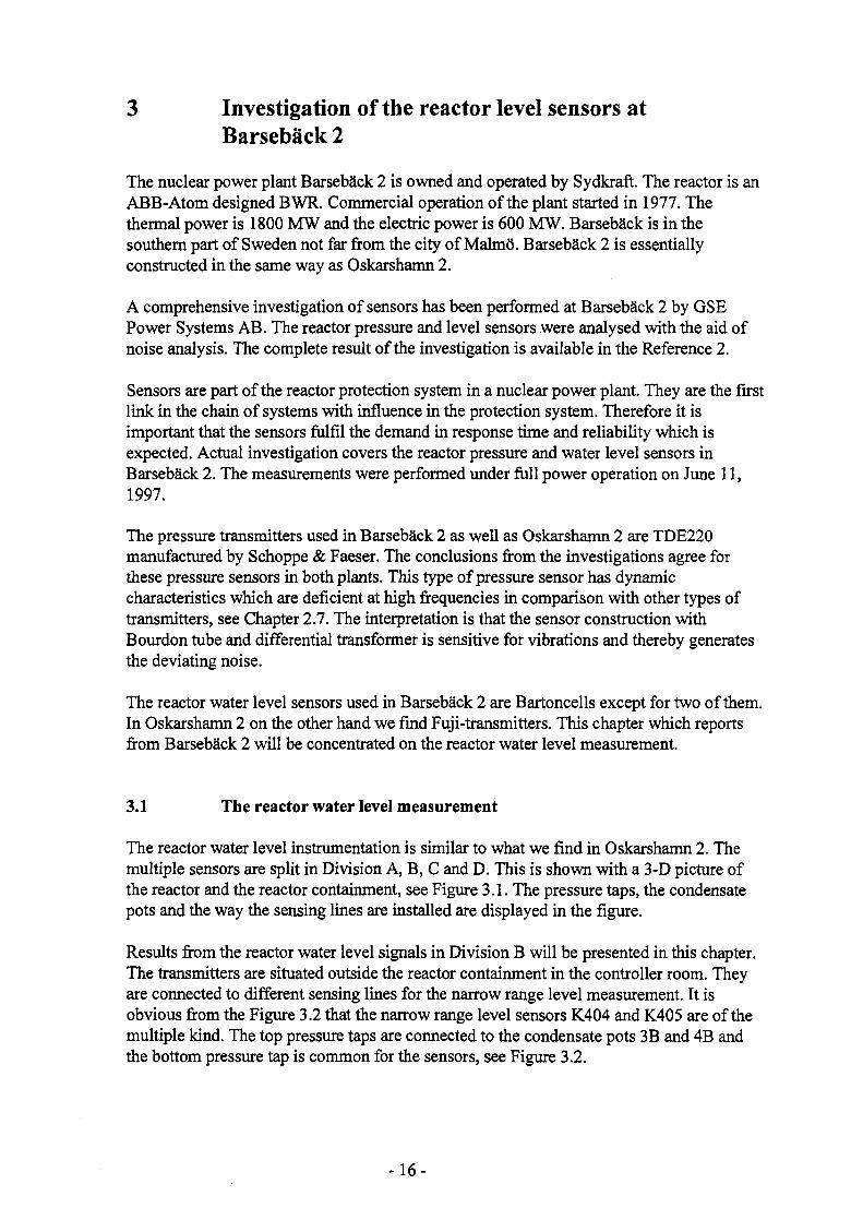
3.1 The reactor water level measurement

The reactor water level instrumentation is similar to what we find in Oskarshamn 2. Themultiple sensors are split in Division A, B, C and D. This is shown with a 3-D picture ofthe reactor and the reactor containment, see Figure 3.1. The pressure taps, the condensatepots and the way the sensing lines are installed are displayed in the figure.

Results from the reactor water level signals in Division B will be presented in this chapter.The transmitters are situated outside the reactor containment in the controller room. Theyare connected to different sensing lines for the narrow range level measurement. It isobvious from the Figure 3.2 that the narrow range level sensors K404 and K405 are of themultiple kind. The top pressure taps are connected to the condensate pots 3B and 4B andthe bottom pressure tap is common for the sensors, see Figure 3.2.

- 1 6 -

The narrow range level sensors K404 and K405 are used for different purposes. K404 isincluded in the protection system while K405 is used in the Feedwater controller.

The wide range level sensor pair K406 and K412 are also multiple sensors. This pair ofsensors have identical sensing lines all the way to the position of the transmitters, seeFigure 3.2.

3.2 The measurements

A comprehensive measurement of reactor pressure and water level signals was performedat Barseback 2 in June 11,1997. The complete result is reported in Reference 2, seeChapter 5. The examples given in this chapter will only exhibit the deviations betweenmultiple water level sensors in Division B in Barseback 2.

3.3 Comparison between narrow range signals K404 and K405

The signals K404 and K405 are displayed as a function of time in Figure 3.3. It is certainfrom this figure that K404 includes a resonance while K405 is clearly damped. The signalsare quite different from dynamic point of view even though K404 and K405 are multiplesensors. APSD for the signals are displayed in the Figure 3.4. This figure confirms a peakat 1 Hz for the K404-signal. The multiple signal K405 shows a spectrum filtered at 0.3 Hz.These transmitters are Bartoncells of the type TDHZ224 for K404 and TDMZ199 forK405.

The deviation in the dynamics between K404 and K405 is puzzling. An inspection of thetransmitters shows that the damping screw is not in the position for damping for any ofthem. This implies that the filtering must be performed outside the transmitter K405.

A possible explanation to the deviations could be so called snubbers - a mechanicalconstriction unit installed in the sensing line to the sensor K405. Such a device causesfiltering of the pressure signal. Another possible interpretation is electronic filtering by thesensor signal.

It should be stressed that the deviation in the dynamics between the narrow range levelsensors K404 and K405 in Division B also is observed with corresponding signals fromDivision A and C. This observation also supports the hypothesis that K405 andcorresponding transmitters in the other divisions (K410 and K415) are filtered knowingly.Such a filtering is, however, not performed for the mentioned sensors in theinstrumentation system in Oskarshamn 2.

- 1 7 -

3.4 Comparison between wide range level signals K406 and K412

The wide range water level transmitters K406 and K412 are multiple sensors. Thesetransmitters have common sensing lines to the position in the controller room, see Figure3.2. The recordings of the signals are presented in Figure 3.5. It is evident that both levelsignals are oscillatory. This is also clear from the APSD curves in the Figure 3.6. Anoscillation at 1 Hz is observed for both signals. There is also a peak at 3 Hz for thetransmitter K406. The level transmitters are Bartoncells of the type TDHZ224 for K.406and TDMZ199 for K412. The interpretation is that the divergence in construction causesthe deviations observed in spectra for the signals.

The construction of the transmitters are visualized in Figures 3.7 and 3.8. The bellow withspring characteristics which is typical for the Bartoncell construction induces largedisplacement in comparison with modern transmitters. The oscillations observed with bothwide and narrow range transmitters is not caused by fluctuations in the reactor water level.The resonance results from an oscillation in the mechanical part of the transmitter. Theresonance system consists of the water in the sensing line together with the springingbellow in the transmitter. This problem is typical for Bartoncells.

The level transmitter Fuji, which is in use in Oskarshamn 2 and for Division D inBarseback 2(K402 and K403), is displayed in the Figure 3.9. The construction of the Fujitransmitter is different. The displacement is less than for the Bartoncell. The 1 Hzoscillations recorded with the Bartoncell is not observed with the Fuji sensor for the levelmeasurements in Barseba"ck 2.

3.5 Conclusions from the investigations in Barseback 2

The analysis of the level sensors from Barseback 2 shows that the Bartoncells in use for thelevel measurement include oscillations. These oscillations do not come from the process.They are generated by the transmitter bellow in interaction with the sensing line water.

APSD for the narrow range level signal K404 includes a peak at 1 Hz. For the multiplenarrow range signal K405 the APSD is filtered already at 0.3 Hz. The deviation in thedynamics is puzzling. An inspection of the transmitters K404 and K405 shows that noextra damping is adjusted for any of the transmitters. This implies that the damping mustbe entered somewhere else.

It should be stressed that the deviation in the dynamics between the narrow range levelsensors K404 and K405 in Division B also is observed with corresponding signals fromDivision A(K409, K410) and Division C(K407, K415). Any low pass filtering for K405,K410 and K415 is not observed in the measurement data from these sensors in Oskarshamn2, see Chapter 2.3. Any interpretation to where the filtering in Barseback 2 is entered is notavailable for the moment.

The experiences from Oskarshamn 2 and Barseback 2 show convincingly that modern levelsensors like Fuji are in better agreement between multiple signals. The investigations also

- 1 8 -

prove that the low frequency oscillations are generated by the Bartoncells and do not existin the Fuji-transmitters.

- 1 9 -

Figure 3.1 Pressure taps, condensate pots and sensing lines for reactor level andpressure measurement. Barseback 2.

Condensating pots

Reactor containment ' Controller room

Figure 3.2 Reactor level measurement in sub B atBarseback 2.

0.19-K4O4 .--K406 .B21V97

Figure 3.3 The narrow range level signals K404 andK405 as a function of time. Barseback 2.

K404 --K40S B2IVS7 -MOB .--K41J .B21V97

Figure 3.4

Freqfffc)

APSD for the narrow range levelsignals K404 and K405.Barseback 2.

Figure 3.5 The wide range level signals K406and K412 as a function of time.Barseback: 2.

-K406 --K412 B2IVS7

Figure 3.6 APSD for the wide range levelsignals K406 och K412.Barseback 2.

©

(5210)

Figure 3.7 Bartoncell Hartmann &Braun TDHZ 224. This unitis in use as K404 och K406 inBarseback 2.

Figure 3.8 Bartoncell Hartmann &Braun TDMZ 199. This unitis in use as K405 och K412 iBarseback 2.

Lwcfe

Lowerasure tide

Figure 3.9

SignalCurrant

iraalos

The transmitter Fuji FFF och FFCwhich is in use in Oskarshamn 2and with two copies atBarseback 2.

4 Experiences from sensor diagnostics at the nuclearpower plant Muhleberg, Switzerland.

The nuclear power plant KKM is a BWR of General Electric design and the reactor type isa BWR4. The power plant is owned and operated by BKW FMB Energie AB. It is locatedat the river Aare in Muhleberg not far from Bern in Switzerland. The reactor has a ratedpower of 1097 MW and the electrical power is 355 MW. The reactor was commissioned in1972. During the years 1992 -1994 a power uprate of 10 % was carried out.

Since 1994 extensive sensor tests are carried out annually at KKM in collaboration withGSE Power Systems AB in Sweden. Reports of significance from these investigations areReferences 3-8 in Chapter 5.

150 sensors have been investigated e.g.: reactor pressure, reactor water level, steam flow,turbine pressure, containment pressure, condenser pressure, turbine building pressure, airpressure for the emergency shut down system, temperature in the torus etc.

Several of the sensors are part of the reactor protection system.

The requirement to investigate the sensors was initiated by an event in 1993 when thereactor pressure suddenly caused a reactor scram during operation.

4.1 Comparisons between multiple signals

In Figure 4.1 the principles for pressure and level measurements at KKM are explained.Condensate pots, sensing lines, and transmitters are shown in the figure. As indicated in thefigure, this construction has only sensing lines on the right and left hand side of the reactor.

Comparisons in both time and frequency domain are used to investigate the characteristicsof the sensors. In Figure 4.2, the reactor level signals are shown with the multiple sensorsML32A1 and ML33A1. These transmitters are connected to the same sensing lines , seeFigure 4.1. As can be seen in the figure the signals are very similar and the deviationsignal, which is also shown in the same figure, is almost a straight line close to zero.

APSD which is calculated for both signals ML32A1 and ML33 Al is graphically displayedin Figure 4.3. There is also a very good agreement between the spectra in the graph.

A similar comparison has been performed for pressure signals, see Figure 4.4 where thepressure signals MP34A2 and MP36A2 are presented as a function of time together withthe deviation between the signals. As can be seen in Figure 4.4 the signals are very similar.These pressure sensors are multiple and furthermore connected to the same sensing line,see Figure 4.1. Corresponding comparison in the frequency domain is shown in Figure 4.5.In this figure the APSD for the multiple signals MP34A2 and MP36A2 are presented. The

- 2 2 -

figure shows that both curves are very similar, even at high frequencies. The type oftransmitter that is used for these pressure signals at KKM is Hartmann & Braun AVC200.

This result should be compared with the lack of agreement between the pressuretransmitters of Bourdon tube TDE220 used at Oskarshamn 2 and Barseback 2.

4.2 A measure to compare signals in time domain

A method has been developed at GSE to quantify the comparison between two multiplesignals in a simple way. The method is called: "Least square fitting analysis for multiplesensors."

Suppose that one of the multiple signals is the input signal Xj and the other the outputsignal Xo. Then calculate the residual X,. based on least square fitting.

X . - K . X . + K.

where Kg = Gain

K, = Offset

The error of the output signal X, gives with the use of Kg, Kothe following expression:

Xr = X0-KgX,.-K0

If the sensor signals are identical, the gain and the offset will adopt the following values:

K g = l a n d K o = 0 .

This agreement will never happen with real signals because they are never completelyidentical. Another measure of agreement between the signals is based on the Ar(Amplitude ratio). The unit is (%) and the function is defined by:

Ar = 100 STD

where STD = Standard Deviation

Gain and Ar are evaluated for the different reactor level transmitter pairs(ML32A1, ML33A1), (ML32A2, ML33A2), (ML32B1, ML33B1) and (ML32B2,ML33B2).

All sensor pairs are connected to the same sensing lines and measures thereby the samedifferential pressure. The connections to the sensing lines and the pressure taps are shownin Figure 4.1.

The results are presented in Figure 4.6, where the gain is shown for the different sensorpairs. The results contain measurements from 1995,1996, extra measurement during

- 2 3 -

autumn 1996 (after reconstruction of the condensate pots) and 1997. The gain is very closeto one for all pairs except for (ML32B2, ML33B2) during the measurement in 1995, seeFigure 4.6. The reason for the deviation is that the level transmitter ML33B2 is notequipped with an internal electronic filter. The mistake occurred during calibration whenthe plant was in regular outage. The lack of filtering implies that the referenced signal willhave an increased noise content.

The amplitude ratios Ar for the corresponding sensor pairs are shown in Figure 4.7. Thisfigure displays a deviation with very high Ar for the sensor pair (ML32B2, ML33B2), seethe measurement 1995. The other sensor pairs have relatively low and even amplituderatios. For the same technical reason as for the deviating Gain parameter mentioned above.The sensor ML33B2 lacks an internal electronic filter.

The Gain and Ar parameters are simple measures on the agreement between multiplesensors. They can therefore be used to follow the historical behaviour of the sensors andindicate deviations as well as trends for the comparisons.

4.3 Evaluation of the dynamics of the density compensation

The reactor water level is measured with a DP transmitter. The principle for the DPmeasurement is presented in Figure 4.8. The height of the water column in the sensing lineup to the level in the condensate pot (+ pressure) is compared with the water level in thereactor (- pressure). The differential pressure is thus the level difference between thecondensate pot and the reactor water level. For that reason it is crucial for the measurementof the water level in the reactor, that the sensing lines are rilled with water and that thelevel in the condensate pot is constant.

The water level signal, which has been registered as differential pressure, is thencompensated for the density. This is done in a special electronic unit. The compensation isdone for P(reactor pressure) and the output signal LEVEL (reactor level) is in the unit(cm). The input signals to the density compensation are DP and P while the output signal isLEVEL. In Figure 4.8 the block diagram for the compensation unit is shown while Figure4.9 presents the DP- signal (ML32A1) and the corresponding LEVEL-signal (ML32A1O).

Except for the numerical compensation, filtering of the DP signal is done in the unit. Thisfiltering can be investigated with the aid of process identification. The DP-signal is judgedas input signal and the LEVEL-signal as the output signal. A mathematical modelARX(Auto Regressive eXogenous)-model is fitted to these time series. The identifiedmodel is exposed for a step disturbance and the time constant for the step result isevaluated. Figure 4.10 shows the step response and the time constant = 81 (ms)which hasbeen calculated for the level transducer ML32A2.

By repeated investigation of the plant's density compensation units concerning filtering, itis possible to detect increasing time delays due to ageing of the electronics. An increasedtime constant implies that a rapid change of the water level is registered with an increasedtime delay.

- 2 4 -

4.4 A 2 Hz peak observed with several sensor signals

During the 1994 sensor investigation, a 2 Hz peak was noted for some of the reactorpressure and water level signals. The oscillation was only observed with some of thesignals, see Figure 4.11. In the simplified block diagram for the instrumentation system atKKM, which is presented in Figure 4.1, it is noted that the 2 Hz oscillation only exists onthe left hand side of the reactor with exception for the level transmitter ML94B, which alsoshows this resonance. The 1994 investigation also showed a high coherence between thereactor pressure and -level at 2 Hz, see Figure 4.12. Considering pure physics the level andpressure signals should not show any form of coherence, due to the fact that the levelsignal measures the differential pressure.

The first hypothesis to explain the existence of a 2 Hz oscillation and the observedcoherence between pressure and level signals was a gas bubble in the common sensing line.Such an error could explain the increased coherence at 2 Hz and the resonance peak inAPSD for the sensor signals.

The inspection during the regular outage in 1994 could not confirm the hypothesis with agas bubble. There must be another reason for the observed resonance at 2 Hz.

4.5 A revised hypothesis for the 2 Hz oscillation

During the measurement in 1995 the number of sensors were increased. The sensors withthe largest oscillation-amplitudes at 2 Hz were ML93 and ML94A, see Figure 4.1. Thesignals are registered as function of time in Figure 4.13. APSD for both signals are shownin Figure 4.14. A large resonance at 2 Hz for ML93 and ML94A is observed in this figure.APSD for ML94B is also displayed in the figure. The curve includes a small peak at 2 Hz.

The revised hypothesis was due to a suspicion that the transmitter-membrane oscillated inone of the level sensors ML93 and ML94A. These transmitters are of the type Hartmann &Braun Barton-Zelle TDHZ224 for ML93 and Hartmann & Braun Membranzelle 050 forML94A, see Figure 3.7 and 4.19 for the principal construction. Via the common sensinglines, a transportation of the oscillations could occur to the other sensors.

The pressure- and level transducers on the right hand side of the reactor have their ownsensing lines which can explain the limitation of the distribution of the resonance. Thecommon sensing lines could explain that the 2 Hz oscillation was observed with as manyas 12 sensors for level and pressure.

The pressure transducers MP30A and MP92 are connected to the sensing lines that provideML93 and ML94A with the differential pressure, see Figure 4.1. The coherence betweenthe pressure signals MP30A and MP92 is shown in Figure 4.15. The coherence is highclose to 1 up to 1 Hz. The phase angle between the signals below 1 Hz is zero degrees. At 2Hz the coherence increases with a peak and corresponding phase angle is 180 degrees. Thepressure signals thus oscillates out of phase at 2 Hz. An oscillating membrane in anyone of

- 2 5 -

the transmitters ML93, ML94A could explain the out of phase phenomena at 2 Hzobserved with the pressure signals MP30A and MP92, see Figure 4.15.

4.6 Experiments with closing of valves

In connection with the 1996 sensor investigation, experiments were carried out to closeValves A and B one at a time during the measurement to study if the oscillations decay, seeFigure 4.1. During the experiment the signals ML93 and ML94A were sampled. Closing ofValve A isolates the sensor ML93 and in the same way, sensor ML94A is isolated whenValve B is closed. The result of this experiment is shown in Figures 4.16-4.17.

When Valve B is closed, sensor ML94A is isolated from the differential pressure in thereactor. In Figure 4.16 APSD for the level signal ML93 is shown during the experimentwith the closing of Valve B. Repeated spectra have been calculated and plotted in thefigure based on measured data before, during and after the closing of the valve. APSD forML93 is not influenced by the isolation of sensor ML94A. The observed 2 Hz resonancecontinues.

Figure 4.17 shows the result with the aid of APSD for ML94A during the experiment withValve A. When the valve is fully open APSD has a clear resonance at 2 Hz and a strongdamping of the frequency content for higher frequencies. After closing the valve, the 2 Hzresonance is distinguished and at the same time the spectra for frequencies higher than 2Hz increase.

The result evidently show that the sensor ML93 generates the oscillations observed by 12sensors for pressure and level which are connected to the common sensing lines. Thetransmitter bellow with springs in ML93 forms together with the mass of water in thesensing line a mechanical system with bad damping, see Figure 3.7. This results in theresonance at 2 Hz. The differential pressure frequencies above 2 Hz, existing via thesensing line, are damped by the mechanical system in the transmitter ML93 as long asValve A is open. When the valve is closed these frequencies appear again in the spectra.

4.7 Replacement of the transmitter ML93

During the outage of the reactor at KKM in the summer 1996, ML93 was replaced by atransmitter of the type Hartmann & Braun Membranzelle 080, see Figure 4.19. This solvedthe problem with the 2 Hz resonance and the damping at higher frequencies disappeared.The new transmitter has a lower displacement and different sensor dynamics and therebythe oscillations have ceased. Figure 4.18 shows APSD for ML93 before and after thechange of the transmitter. Both curves clearly show that the 2 Hz resonance is wiped outand that the damping at high frequencies are recovered after the replacement of thetransmitter.

- 2 6 -

4.8 Investigation of the temperature sensors in the torus

Below the reactor there is a water filled torus shaped suppression pool, which is used inconnection with emergency cooling. Steam can be transferred down into the torus to becondensated during an emergency. To supervise the torus, 12 temperature sensors and 4average temperatures which are calculated from the recorded temperatures, are used. Thetemperature sensors which are mounted in a thermowell in the torus are of the typeRTD(Resistance Temperature Detector).

The temperature in the torus is constant around 22 degrees. It does not contain any naturalfluctuation as the water volume is so large. Therefore one experiment with eachtemperature sensor is carried out to investigate the dynamics. The individual temperaturesensor is dismounted from its thermowell and entered into a bucket with ice and water.During the experiment, the temperature and the average temperature signals are sampled.

As soon as the temperature is stable at zero degrees the temperature sensor is dried up andremounted again into its position in the thermowell. Then the temperature naturallyincreases up to its original position. It is interesting to notice that the temperature decreasesexponentially towards zero degrees when the RTD-element is entered into the ice. The timeconstants are calculated from the sampled time series with classical methods. In Figure4.20 the experiment is shown when the temperature sensor MT205A is entered into ice andwater. At the time 200 (s), the temperature decreases from 22 degrees to zero degrees. Thetime constant is calculated to 7.4 (s). This time constant is determined by the heat transferto the RTD-element and the dynamics for the electronic conversion of the temperature. Thethermal resistance between the cooling water and the RTD-element is in this caseneglectable.

When the element is remounted into its position in the torus the temperature increaseoccurs with a time constant which is considerably larger, see Figure 4.20. In this case thetime constant has been calculated to 60 (s). The reason for the larger time constant is thatthe thermal resistance between the thermowell and the RTD-element is added to thedynamics.

The experiment with the cooling and heating of the RTD-element and determination of thetwo time constants answers the following questions:

• The cooling time constant answers the question: Is the response time relevant for theRTD-element with additional electronics? In this case 7 (s).

• The heating time constant answers the question: Does any extra thermal resistance(rubbish or oxide) exist between the RTD-element and the thermowell with influence onthe response time? In this case 60 (s).

The average temperature is a result of electronic summation. With the aid of three torustemperature signals an average temperature is formed. In Figure 4.20 the averagetemperature MT905A, which is formed by MT205A and two other temperature signals, isshown.

-27-

When the experiment with cooling and heating of MT205A occurs the averagetemperature MT905A will naturally be affected. As shown in Figure 4.20 MT905Adecreases from 22 degrees down to 14.6 degrees because the average value at cooling ofone RTD is calculated as the average of the three temperatures (0, 22,22) degrees = 14.6degrees, see Figure 4.20.

The function of the electronics for the average temperature can also be investigated withthe aid of signals from the experiment. Besides that the average temperature shall fluctuatebetween 22 degrees and 14.6 degrees it is also expected that the time constants of coolingand heating shall be the same as for the individual RTD-element. This is actually the casefor MT905A, time constant at cooling = 7.6 seconds and at heating = 58.5 seconds. Thisimplies that the electronics which forms the average temperature works correctly.

4.9 Conclusions from the investigations at Kernkraftwerk Muhleberg

Comprehensive investigations of sensors are performed annually at KKM by GSE PowerSystems AB. Approximately 150 sensors are analyzed with respect to the dynamiccharacteristics. The methods used are based on noise analysis.

The experiences from KKM show convincingly that the results from the multiple sensoranalysis can be compared when the investigations are repeated annually. Measures likeGain and Ar can be studied over the time and deviations from the comparison of historicaldata can be displayed. One example shows how the lack of an electronic filter in atransmitter influences the statistics.

Outside the investigation of the transmitter characteristics, analysis is also performed forthe density compensation units. The filtering effect in such a unit can be calculated as atime constant. The method used is process identification. Measurement data estimate thetime constant to 81 (ms).

A 2 Hz resonance was observed with 12 sensors for reactor pressure and reactor water levelin 1994 and 1995. It was proven via experiments that the source to the oscillation was aBarton-Zelle TDHZ224 used for the reactor water level measurement. The transmittermembrane oscillates thereby influencing on the other sensors for pressure and level via thecommon sensing lines. The oscillations cease when the transmitter is replaced with aMembran-Zelle 080.

Under the reactor at KKM, a torus shaped water suppression pool is placed which is part ofthe emergency cooling system. Supervision of the water temperature is performed with anumber of temperature sensors. The dynamics of these sensors are estimatedexperimentally as time constants during cooling and heating of the sensors. Deviatingsensors can be discovered with the aid of this method.

- 2 8 -

Sensing line

MP34A1 MP36A1 MP34B1 MP36B1

2Hz 2Hz 2Hz 2Hz

ML32A1 ML33A1 ML32B1

2HzML33B1 MP30A

MP922Hz 2Hz

ML93I

rML94A

fii

2Hz

•B

Nil A NUB

Reactor

N16A N16B

Condensating

MP34A2 MP36A:;

MP30B

MP34B2 MP36B2

ML32A2 ML33A2

<2HzML94B

ML32B2 ML33B2

r-t

Figure 4.1 Reactor water level and reactor pressure sensors at Kernkraftwerk Mtihleberg.

1

0 3

•0.5

.1

• 1 J i i o

ml32a1

A i l i

I20 30

.ml33«1

40

,(ml32a1 -rr

wyruiIf

so eo

D33«1 ) ,KKMA

I I

I

70 80 BO 1C

-mt32«1 -^71133.1 KKMA

Tlni»(.)

Figure 4.2 Reactor level signals ML32A1, ML33A1and the difference between the signals as afunction of time. Kernkraftwerk MUhleberg.

Figure 4.3 APSD for the reactor level signals ML32A1and ML33A1. Kernkraftwerk Mtlhleberg.

MP34A2 .MPMA2 .(MP34A2 -MP38A2 ),KKMCS7

40 SO 60 70 80 90 100

Figure 4.4 Reactor pressure signals MP34A2,MP36A2 and the deviation between thesignals as a function of time.Kernkraftwerk Mtlhleberg.

10°

to-1

MP34A2 « MP38A2 ofKKMC97

1C«

104

10"'

10*10*

Figure 4.5

F«q(Hz)10' 102

APSD for the reactor pressure signalsMP34A2 and MP36A2. KernkraftwerkMtShleberg.

Multiple sensor bealdi test «t KKM; ML32,33 GainMultiple sensor health test al KKM; ML32,33 Amplitude Ratio

Figure 4.6 Gain for the level sensor pairs(ML32A1, ML33A1), (ML32A2, ML33A2),(ML32B1, ML33B1), (ML32B2, ML33B2)estimated with data from 1995-1997.Kernkraftwerk Mtlhleberg.

Reac to r

^ " ~ ) Condensa t ingpo t

Sens ing l ine

Reactor containment

ML32A1MU3A1

ML32A2ML33A2

ML32B1ML33B1

ML32B2ML33B2

9596MA97

ISM««A97

9596

97

96A97

0

•••

20 40 60Amplitude Ratio [%|

80 10

Figure 4.7 Ar for the level sensor pairs(ML32A1, ML33A1),(ML32A2, ML33A2),(ML32B1, ML33B1), (ML32B2, ML33B2)estimated with data from 1995-1997.Kernkraftwerk Mtihleberg.

Pressuretransmitter

\ P

FH Leve l

L e v e l Dens i tyt ransmi t te r compensa t ion

Figure 4.8i i

Principal drawing for the level measurement and density compensation. KernkraftwerkMtlhleberg.

0 1 2 > 4 5 « 7 » » 1 0

Figure 4.9 DP-signal and level signal forthe sensor ML32A1.Kernkraftwerk Mtlhleberg.

Op*n top ttaprapora* from mS2>1 tomoaio; Mo-38 FH.; KKMA

0 OS 1 15 2 2.5 3 S.S 4

Figure 4.10 Step response of the identified model.Time constant = 81 ms. KernkraftwerkMtihleberg.

Cohtranc* t*twwn ml32a1 and MPS2 FU: KKMA

Figure 4.11 A resonance at 2 Hz is visiblewith the level signals(ML32A1, ML33A1) but notwith (ML32A2, ML33A2).Kernkraftwerk Mtthleberg.

Figure 4.12 The coherence-function between the levelsignal ML32A1 and the pressure signalMP92. Kernkrafrwerk Mtihleberg.

0 1 I J 4 6 » 7 » » 1 0

O 1 2 3 4 5 » 7 » B 1 0

Figure 4.13 The reactor level signalsML93 and ML94A as afunction of time.Kernkraftwerk Mlihleberg.

Figure 4.14 APSD for ML93, ML94A andML94B. KernkraftwerkMtlhleberg.

10 10'FlKhkmli.dal Hz

Figure 4.15 Coherencen between reactorpressure signals MP92 och MP30A.Kernkraftwerk Muhleberg.

10° 101 10s

F«|(H2)

Figure 4.17 APSD for ML94A when the valve Ais moved from open to closedposition. The resonance at 2 Hz isceased. ML93 is the reason to theoscillation. KernkraftwerkMiihleberg.

.2

10J

10"

10J

10*

10J

10-

APS0ML93

Bopen v

10"'

Figure 4.16

10° 10- Freq(Hz) « -

APSD's for the signal ML93 whenvalve B is moved from open toclosed position. The sensor signal isnot influenced. The resonance at 2Hzcontinous. Kernkraftverk Miihleberg.

m«3 KKMS--ML93 KKMC

Before exchange of ML33March -96

10-Iff1

Figure 4.18 APSD for ML93 before and after theexchange of transmitter.Kernkraftwerk Muhleberg.

Figure 4.19 The level transmitter ML93 wasexchanged with thisMembranzelle 080 and theoscillation stopped.Kernkraftwerk Mtthleberg.

.([ VfI I

400 600 600

Figure 4.20 Experiment with thetemperature sensors in torus.The RTD-element isdismounted and cooled in abucket of ice and water. Afterthat reinstalled again in torus.Kernkraftwerk Muhleberg.

5 Acknowledgements

Special thanks are given to Mr. Sune Jonsson at Oskarshamn 2, Mr. Jan Ove Andersson atBarseback 2 and Mr. Herbert Schwaninger at Kernkraftwerk Mtthleberg who gave thepermission to publish the report.

Thanks also to the Swedish Nuclear Power Inspectorate who sponsored the activity to writethe report.

- 3 3 -

6 References

1 Bergdahl BG, Kubota O and Sandell S. Sensor tests at Oskarshamn 2, Basedupon measurements from September 24,1997. GSE-97/17.(in Swedish)

2 Bergdahl BG and Sandell S. Investigation of transmitters at Barseback 2.Based upon measurements from June 11,1997. GSE-97/15.(in Swedish)

3 Bergdahl BG, Oguma R and Schwaninger H. Sensor tests at KernkraftwerkMuhleberg, Switzerland. 24-25 Feb. 1994. EuroSim-94/8.

4 Bergdahl BG, Liao B, Oguma R, Schwaninger H. Sensor tests atKernkraftwerk Miihleberg, Switzerland. 3 - 6 April 1995. EuroSim-95/24.

5 Bergdahl BG, Sandell S, Kubota O and Schwaninger H. Sensor tests atKernkraftwerk Mtihleberg, Switzerland. Measurement on 19 - 22 March1996. EuroSim-96/08.

6 Bergdahl BG, Liao B, Oguma R, Schwaninger H. Sensor diagnostics in aB WR based on noise analysis. An invited paper presented at the NPIC &HMIT'96 meeting May 6 - 9,1996, The Pennsylvania State University, USA.

7 Bergdahl BG, Schwaninger H. Sensor tests at Kernkraftwerk Muhleberg,Switzerland. Measurement on 11-12 Sept. 1996. GSE-96/16.

8 Bergdahl BG, Oguma R, Kubota O, Schwaninger H. Sensor tests atKernkraftwerk Miihleberg, Switzerland. Measurement on 17-20 March 1997.GSE-97/9.

9 Bergdahl BG and Oguma R. Health test of 99 sensors at Ringhals 3 and 4with the aid of noise analysis. Paper presented at the 21th IMORN,September 20-22,1989, Paul Scherrer Institute, Villigen, Switzerland.EuroSimAB 1990-10-24.

10 Hashemian HM et al. Effect of Ageing on Response Time of Nuclear Plantpressure Sensors. Analysis and Measurement Services Corporation.NUREG/CR-5383.

11 Hashemian HM et al. Long Term Performance and Ageing Characteristics ofNuclear Plant Pressure Transmitters. Analysis and Measurement ServicesCorporation. NUREG/CR-5851.

- 3 4 -

STATENS KARNKRAFTINSPEKTIONSwedish Nuclear Power Inspectorate

Postadress/Postal address Telefon/Telephone Telefax

SKIS-106 58 STOCKHOLM

Nat 08-698 84 00Int +46 8 698 84 00

Nat 08-661 90 86Int +46 8 661 90 86

Telex

11961 SWEATOMS