investigation of future flow reducer sizes in houses added
TRANSCRIPT

University of South FloridaScholar Commons
Graduate Theses and Dissertations Graduate School
10-20-2016
Investigation of Future Flow Reducer Sizes inHouses Added to an Existing Gravity Flow WaterSystem to Ensure its SustainabilityMichelle RoyUniversity of South Florida, [email protected]
Follow this and additional works at: http://scholarcommons.usf.edu/etd
Part of the Civil Engineering Commons
This Thesis is brought to you for free and open access by the Graduate School at Scholar Commons. It has been accepted for inclusion in GraduateTheses and Dissertations by an authorized administrator of Scholar Commons. For more information, please contact [email protected].
Scholar Commons CitationRoy, Michelle, "Investigation of Future Flow Reducer Sizes in Houses Added to an Existing Gravity Flow Water System to Ensure itsSustainability" (2016). Graduate Theses and Dissertations.http://scholarcommons.usf.edu/etd/6580

Investigation of Future Flow Reducer Sizes in Houses Added to an Existing Gravity Flow Water
System to Ensure its Sustainability
by
Michelle Roy
A thesis submitted in partial fulfillment of the requirements for the degree of
Master of Science in Civil Engineering Department of Civil and Environmental Engineering
College of Engineering University of South Florida
Major Professor: James R. Mihelcic, Ph.D. Mauricio Arias, Ph.D. Kenneth Trout, Ph.D.
Date of Approval: October 14, 2016
Keywords: NeatWork Design, Rural Gravity Flow Water Supply and Distribution, Aqueduct Ex-pansion, Sustainable Development Goals
Copyright © 2016, Michelle Roy

Acknowledgments
I would personally like to thank everyone involved that made the completion of this thesis
possible.
First and foremost, my principal advisor Dr. Jim Mihelcic for his leadership and dedica-
tion to the Master’s International Program at USF. Also, for his guidance and continual support
during my time as a Peace Corps Volunteer and as a researcher.
My graduate committee, Dr. Mauricio Arias and Dr. Kenneth Trout for their feedback and
help.
My beloved Peace Corps community of Santa Cruz, especially the local water commit-
tee. They partnered with me to survey the system providing the initial data required for this re-
source. Their interest and willingness to fabricate and install flow reducers in the system as well
as providing feedback on the tools I created was essential.
My family and friends for their loving support while I was away serving as a Peace Corps
Volunteer, especially my sister, Julie Mulherin, and my mom, Dee Cameron.
This material is based upon work supported by the National Science Foundation under
Grant Nos. 0966410 and 1243510. Any opinions, findings, and conclusions or recommendations
expressed in this material are those of the author and do not necessarily reflect the views of the
National Science Foundation.

i
Table of Contents
List of Tables .............................................................................................................................. iii List of Figures ............................................................................................................................. v Abstract..................................................................................................................................... vii Chapter 1: Introduction ................................................................................................................ 1
1.1 Importance of Potable Water ..................................................................................... 1 1.2 Gravity Flow Aqueducts ............................................................................................. 3 1.3 Water Access in Panama ........................................................................................... 3 1.4 Peace Corps in Panama ............................................................................................ 4 1.5 Peace Corps Master’s International Program ............................................................ 5 1.6 Flow Reducers........................................................................................................... 5 1.7 Background Information on Intended Santa Cruz Aqueduct ....................................... 8 1.8 Motivation ................................................................................................................ 10 1.9 Objectives ................................................................................................................ 11
Chapter 2: Literature Review ..................................................................................................... 13
2.1 Aqueduct Design ..................................................................................................... 13 2.1.1 Fluid Mechanics Related to Thesis Research ............................................ 13 2.1.2 Water Distribution Systems in the Developed World .................................. 18 2.1.3 Water Distribution Systems in the Developing World ................................. 20
2.2 NeatWork and its Design Principles ......................................................................... 27 2.2.1 Design Phase ............................................................................................ 27 2.2.2 Simulation Phase ...................................................................................... 31
Chapter 3: Materials and Methods ............................................................................................ 33
3.1 Making a Water Level .............................................................................................. 33 3.2 Data Collection and Organization ............................................................................ 34 3.3 Procedure for Analyzing Sample Aqueduct .............................................................. 36 3.4 Testing Rules from Analysis ..................................................................................... 41
Chapter 4: Results and Discussion ........................................................................................... 44
4.1 Analysis of Sample Aqueduct ................................................................................... 44 4.2 Analysis of Experiment Houses to Test Rules from Aqueduct Analysis..................... 58 4.3 Audience for Decision Support Tool ......................................................................... 60 4.4 Assumptions ............................................................................................................ 61 4.5 Tool to Size Flow Reducers ..................................................................................... 61 4.6 Applying the Tool to the As-Built Aqueduct ............................................................... 63
Chapter 5: Conclusions and Recommendations ........................................................................ 70
5.1 Conclusions from Objective 1 .................................................................................. 70 5.2 Conclusions from Objective 2 .................................................................................. 71 5.3 Conclusions from Objective 3 .................................................................................. 72

ii
5.4 Recommendations for Future Research .................................................................. 73 List of References ..................................................................................................................... 78 Appendix A: Peace Corps Volunteer Guide to Sustainable Flow Reducer Projects ................... 83 Appendix B: NeatWork Topography Input Tables for “As Is” and “All” Files .............................. 101 Appendix C: NeatWork Simulation Results ........................................................................................ 119 Appendix D: NeatWork Inputs Topography and Simulation Reults for Final Design ................. 131 Appendix E: Calvulations of Available Head at Each Faucet ................................................... 143 Appendix F: Determining an Appropriate Number of Future Connections................................ 151 Appendix G: Copyright Permissions ........................................................................................ 153
iii
List of Tables
Table 1: Minor Headloss Coefficients (K) for Various Aqueduct Components Obtained from Crowe et al. (2010) ..........................................................................................16
Table 2: Summary of Computer Software for the Design of Distribution Networks Used
in the Developed World ............................................................................................18 Table 3: Summary of Relevant Master’s International Reports and Theses on Design
and Construction of Gravity Flow Water Systems ....................................................21 Table 4: Recommended Maximum and Minimum Pressure at Faucets in a Gravity Flow
Distribution System ..................................................................................................24 Table 5: Recommended Maximum and Minimum Flow Rates at Faucets in a Gravity
Flow Distribution System .........................................................................................25 Table 6: Suzuki’s (2010) Ranking Criteria for a Distribution Lines..........................................26 Table 7: Distribution of Results from Suzuki (2010) Study for Distribution Lines ....................26 Table 8: Input and Output for NeatWork’s Design Phase .......................................................28 Table 9: Flows and Probabilities Used in the Calculation of the Service Quality Factor in
NeatWork.................................................................................................................30 Table 10: Comparing Headloss Values through Orifices ..........................................................31 Table 11: Design Input Criteria for Design of Sample Aqueduct ..............................................37 Table 12: Flow Reducer Sizes for Design File Based on Flow Reducers Size of the
Closest House .........................................................................................................39 Table 13: Summary of NeatWork Design Files Used to Analyze the Santa Cruz Aqueduct ......39 Table 14: Differences in Determined Pipe Sizes from NeatWork between “As Is” Design
and “All” Design .......................................................................................................45 Table 15: Total Length of Pipes Changed between “As Is” Design and “All” Design ................46 Table 16: Differences in Flow Reducer Sizes between “As Is” Design and “All” Design ...........47 Table 17: Notable Changes between Designs for Sample Aqueduct in Minimum Flow and
Percentage of Time Below 0.1 L/s ...........................................................................47 Table 18: Connections with Greater than 0.3 L/s when Flow Reducers are Not Installed ........48
iv
Table 19: Flow Reducer Sizes, Relative Altitudes, Length of Pipes between Tank and Faucet for Santa Cruz Aqueduct, Available Head, Average Pressure, and Maximum Pressure ..................................................................................................50
Table 20: Calculated Available Head, Average Pressure from NeatWork Simulation, and
Maximum Pressure from NeatWork Simulation for Each Faucet ..............................51 Table 21: Ranges of Calculated Head, Average Pressure, and Maximum Pressure for
Different Flow Reducer Sizes ...................................................................................53 Table 22: Comparison of Flow Reducer Size Based on the Closest House and from the
NeatWork Design .....................................................................................................54 Table 23: Variations Simulation Flow Results Corresponding to Different Flow Reducer
Sizes from Prediction, NeatWork Sized, and Based on Closest House ....................60 Table 24: Simulation Differences between Varying Flow Reducer Sizes for House 6 in
As-Built Aqueduct ....................................................................................................66 Table B1: Node Node Input Table to Create NeatWork “As Is” Topography File……………… 101 Table B2: Arc Length Input Table to Create NeatWork “As Is” Topography File ...................... 105 Table B3: Node Imput Table to Create NeatWork “All” Topography File ................................. 109 Table B4: Arc Length Input Table To Create NeatWork “All” Topography File ......................... 114 Table C1: NeatWork Simulation Results for "All" Design File ................................................. 119 Table C2: NeatWork Simulation Results from "As Is" Design File .......................................... 121 Table C3: NeatWork Simulation Results for “All As Is Sizes” Design File ............................... 123 Table C4: NeatWork Simulation Results for “All As Is Sizes No Discs” Design File ................ 125 Table C5: NeatWork Simulation Results for “All As Is Sizes Discs 396” Design File ............... 127 Table C6: NeatWork Simulation Results for “All As Is Sizes Discs Closest” Design File ......... 129 Table D1: Node Input Table to Create NeatWork “Final Design” Topography File .................. 131 Table D2: Arc Length Input Table to Create NeatWork “Final Design” Topography File .......... 135 Table D3: NeatWork Simulation Results for “Final Design” Design File .................................. 140 Table E1: Spreadsheet Used to Calculate Available Head at Each Faucet……………. .......... 143

v
List of Figures
Figure 1: Schematic of How and Where a Flow Reducer is Installed in a Pipe ........................ 7 Figure 2: Map Showing where Santa Cruz is Located within Panama and where Key Aqueduct Components are Located within Santa Cruz. ............................................ 9 Figure 3: Map of Confirmed Connections and Potential Connections with Faucet Numbers for Santa Cruz Aqueduct (not to scale) .....................................................10 Figure 4: Sample Hydraulic Grade Line (HGL) .......................................................................15 Figure 5: Screenshot of NeatWork's Design Parameter Input Section That Shows Required Inputs and Default Values .........................................................................28 Figure 6: Screenshot of Simulation Parameter Inputs in NeatWork .........................................32 Figure 7: A Completed Water Level ........................................................................................33 Figure 8: Pictures from when the Author Surveyed in the Field ...............................................35 Figure 9: Screenshot of NeatWork Input Tables to Create a New Topography ........................35 Figure 10: Map Including Experiment Houses to Test Developed Rules for Sizing Flow
Reducers Showing Flow Reducer Sizes and Faucet Numbers from “All” Design (not to scale) ............................................................................................................42 Figure 11: Location of Faucets as Indicated in the Red Circles where the Flow Reducer Size Changes when the Design Changes from the “As Is” Design to the “All” Design (not to scale) ................................................................................................46 Figure 12: Map of Flow Reducer Sizes and Faucet Numbers from “All As Is Sizes” Design File (not to scale) .....................................................................................................49 Figure 13: Map of Faucet Locations as Indicated in the Red Circles where Flow Reducer Size Changes from that of Closest House and Ideal Size from NeatWork Design (not to scale) ................................................................................................55 Figure 14: Profile of Aqueduct for Houses 24-29 with Flow Reducer Sizes Indicated (in inches) .....................................................................................................................56 Figure 15: Profile of Aqueduct for Houses 43-45 with Flow Reducer Sizes Indicated (in inches) .....................................................................................................................56

vi
Figure 16: Profile of Aqueduct for Houses 58-60 with Flow Reducer Sizes Indicated (in inches) .....................................................................................................................57 Figure 17: Profile of Aqueduct for Houses 10-16 with Flow Reducer Sizes Indicated (in inches) .....................................................................................................................57 Figure 18: Final Decision Support Tool Created for the Originally Designed Santa Cruz
Aqueduct Presenting Faucet Numbers and Locations where Flow Reducers Cannot Be Sized Based on the Flow Reducer Size of the Closest House (not to scale) ...................................................................................................................62 Figure 19: Map of As-Built Gravity Flow Water System in Santa Cruz with House Numbers and Flow Reducer Sizes from Final Designs (not to scale) ......................................65 Figure 20: Map with House Numbers and Flow Reducer Sizes Provided to the Santa Cruz
Water Committee (not to scale) ...............................................................................68 Figure 21: Picture of Extra Flow Reducers Provided to the Santa Cruz's Water Committee......69
vii
Abstract
Goal 6 of the United Nations Development Program’s new Sustainable Development
Goals aims to ensure availability of clean water and sustainable management practices to all by
the year 2030. Peace Corps Panama partners with communities in order to help provide sus-
tainable water solutions to communities in need. Water, Sanitation, and Hygiene (WASH) Vol-
unteers spend at least two years living in a community to identify and implement solutions to
water problems and train local water committees on how to maintain their improved systems. A
common solution for unequal distribution of flow in the distribution network of a gravity flow wa-
ter system is through the installation of flow reducers before each faucet. These can be sized
with the help of NeatWork, a free, downloadable compute software. In Panama, flow reducers
(also referred to as orifices) are manufactured to create a perforated plastic diaphragm fitting
placed in the distribution pipe or union section upstream of a faucet. They help ensure longevity
of the aqueduct by balancing the flows between houses, thus, enabling continuous water flow
for all users. An important characteristic of flow reducers is that while they can be installed in
new water systems, they can also be installed in existing systems to fix inequalities from inade-
quate original designs or extensions to the systems. However, little guidance exists for volun-
teers or communities to ensure the sustainability of these projects. Accordingly, the object of
this thesis was to investigate how adding houses to existing aqueducts would affect its servicea-
bility and how to determine a way for communities to size the flow reducers for future houses.
The existing gravity flow water system in Santa Cruz, Panamá was surveyed including
all the potential houses which were then analyzed using NeatWork. The results demonstrate
that while it is better to include all potential locations during the initial survey, if it expands at an
viii
average growth rate, additional houses may decrease serviceability, but in a negligible way that
will not affect the overall reliability of the distribution system.
Utilizing NeatWork, this research showed it is able to determine ideal sizes of flow reduc-
ers for additional houses that could be added. Patterns were identified and used to simplify flow
reducer sizing so that community members could do it themselves. While most of the time, the
ideal flow reducer size for a new house will be the same size as the flow reducer size that is in-
stalled in the closest house that is already connected to the aqueduct, sometimes this is not the
case. This typically occurs towards the end of branches and in areas where not all flow reducer
sizes are present. These areas are clearly identified to the water committee on a map of the
distribution system that was provided to various water committee members. With this map and
simple instructions, the Santa Cruz water committee can continue correctly adding flow reduc-
ers to new houses.
Through the research of this thesis, fabricating and installing flow reducers in the Santa
Cruz water distribution system, and working alongside community members many lessons were
learned about flow reducers and best practices. This knowledge has been converted into a
guide about sustainable flow reducer projects. It has been left with current volunteers and the
director of training for the WASH sector of Peace Corps Panama so that the volunteers can
adapt the developed tools in their own communities.

1
Chapter 1: Introduction
1.1 Importance of Potable Water
In 2000, the United Nations (UN) created the Millennium Development Goals (MDGs) to
meet the needs of the world’s poorest. The importance of clean water is emphasized in Goal
7.C: “Halve, by 2015, the proportion of people without sustainable access to safe drinking water”
relative to the year 1990 (United Nations, 2015). Later in 2010, the UN General Assembly
declared water a basic human right (United Nations, 2010). Despite the global efforts, in 2015,
663 million people still lacked access to an improved drinking water source with the majority
living in rural areas (United Nations, 2015, UNICEF and WHO, 2015).
More work needs to be done to continue increasing water coverage among the poor and
to ensure the sustainability of completed water projects. The United Nations Development
Program (UNDP) recognizes this and has included water as Goal 6 of the new Sustainable
Development Goals (SDGs) that were created in September 2015 to replace the MDGs.
Specifically, Goal 6 is to “ensure availability and sustainable management of water and
sanitation for all” by the year 2030 (United Nations Development Program, 2015). Other SDGs
indirectly depend on access to water.
One way to reduce the 663 million underserved people is by providing piped water on
premises, or water that is piped to a dwelling, yard, or plot (UNICEF and WHO, 2015). While
this option has been associated with the best health outcomes, only 58% of the world’s
population currently utilizes piped water (United Nations, 2015, UNICEF and WHO, 2015).
However, just because one has access to piped-water does not guarantee they have access to
reliable, potable water. For example, water quality is not taken into account when determining if
a water system is “improved” and often services are intermittent, creating more health risks

2
(Schweitzer and Mihelcic, 2012, UNICEF and WHO, 2015). In fact, at a minimum, while still
accounting for 8 hours of suspended service, a properly functioning gravity flow water system
should operate for 16 hours a day (Schweitzer and Mihelcic, 2012). The World Bank evaluated
their water and sanitation projects, which encompass larger and more complicated types of
projects such as urban water and sewage systems, that closed between 1990 and 2001 and
only 64% were reported to be satisfactory and less than half were deemed likely to be
sustainable (World Bank, 2003). Schweitzer and Mihelcic (2012) developed and tested a
framework to assess how likely a rural water system in the Dominican Republic was to be
sustainable and found that for 18% of the systems, it was unlikely the community will be able to
overcome a significant challenge to maintain adequate access to water. Accordingly, it is
necessary to continue to improve existing aqueducts and working to make sure communities
understand how to maintain and operate their aqueduct systems.
Schweitzer (2009) defined sustainability for a rural community water system as one that
provides “1) equitable access amongst all members of a population to continual service at
acceptable levels (quantity, quality, and access location) providing sufficient benefits (health,
economic, and social) and 2) requires reasonable and continual contributions and collaboration
from service beneficiaries and external participants.” Furthermore, the aqueduct should provide
water for at least 16 hours per day (Schweitzer, 2009; Schweitzer and Mihelcic, 2012). It is
important, to keep the system operating at capacity at all times because people are reluctant to
pay for intermittent service and continuous supplies are safer (Lee and Schwab, 2005). Also,
increased quantities of water are known to improve health through providing access to improved
sanitation and hygiene (Mihelcic et al., 2009) and can specifically reduce diarrhea by 20-25% as
it allows for better hygiene practices (Fry et al., 2010).

3
1.2 Gravity Flow Aqueducts
Gravity flow water distribution systems (also referred to as aqueducts) are an
appropriate way to provide developing communities piped water. Typically, they have low
operation and maintenance associated with them since no mechanical energy (e.g., via pumps)
is required (Mihelcic et al., 2009). A typical gravity flow system collects water from the source, a
spring or river, through an intake structure. It is then carried through a conduction line into a
storage tank. From the tank, water flows into the community through a distribution network
which can have multiple branches that end at faucets. These faucets provide the users with
their basic water needs. More information about the design and construction of each
component can be found in A Handbook of Gravity-Flow Water Systems (Jordan, 1984) and
Field Guide in Environmental Engineering for Development Workers (Mihelcic et al., 2009).
There is also much detail in the many research documents generated by the Master’s
International Peace Corps Program (e.g., Reents, 2003; Niskanen, 2003; Simpson, 2003; Annis,
2006; Good, 2008; Schweitzer, 2009; Suzuki, 2010; Orner, 2011: Yoakum, 2013). These
resources suggest the engineer would rely primarily on placement of different size pipe
combinations and globe valves to obtain the appropriate amount of water at each tapstand.
However, there is very little information found in this and other literature on how to properly use
flow reducers in a rural gravity flow water system.
1.3 Water Access in Panama
Panama has a large wealth distribution as shown by the relatively high GINI index of
51.9 where 0 represents perfect equality and 100 represents total inequality (World Bank,
2014). Furthermore, 27% of the population is living in poverty (CIA, 2014) and 14.2% are living
in extreme poverty (Guillén, 2012). In contrast, 98% of the country’s population has access to
an improved water source (UNICEF and WHO, 2015). Unfortunately, this percentage
decreases to 89% in rural areas (UNICEF and WHO, 2015). Furthermore, the worst coverage

4
rates in Panama are found in the indigenous rural areas where only 47.6% of people have
potable water (Guillén, 2012)
Gravity flow water systems are one type of improved water source being used in
Panama (Guillén, 2012). Panama’s mountainous geography and abundant rainfall during the
rainy season make it a likely place for gravity flow aqueduct systems. This is one reason why
almost all of Panama’s rural populations with a safe-water source (89%) have piped water on
premise (83%) (UNICEF and WHO, 2015).
These water systems are maintained by local governing bodies formally known as
Juntas Administrativas de Acueductos Rurales (JAAR) which translates to the Administrative
Boards of Rural Aqueducts. However, they are more commonly referred to as Directivas in
Spanish or Water Committees in English. They consist of seven elected people from the
community who are responsible for the administration, operation, and maintenance of the
aqueduct (MINSA, 1994). While these people are responsible for ensuring the sustainability of
the aqueduct, no technical experience is required (MINSA, 1994).
1.4 Peace Corps in Panama
The Peace Corps started working in Panama in the Environmental Health sector, now
renamed Water, Sanitation, and Hygiene (WASH) in 2002. Since its creation, more than 215
Peace Corps Volunteers have served in communities working towards the following objectives:
1) train community members to increase participation, organization, and capacity for sustainable
projects, 2) educate community members to prevent water borne disease transmission, 3) train
water committees how to operate, maintain and manage potable water and sanitation systems,
and 4) construct, improve, or rehabilitate water systems (Redmond, 2012).

5
1.5 Peace Corps Master’s International Program
Peace Corps Volunteers are now able to combine their training and service with
graduate education through Master’s International (MI) (Mihelcic et al., 2006; Hokanson et al.,
2007; Mihelcic, 2010; Manser et al., 2015). The author of this thesis was enrolled in a Master’s
International program and that particular program requires a research thesis as part of the
graduate degree requirements. Examples of water-related research theses performed by Peace
Corps Volunteers in Panama include Embodies Energy Assessment of Rainwater Harvesting
Systems in Primary School Settings on La Peninsula Valiente, Comarca Ngöbe Bugel, Republic
of Panama (Green, 2011), Post-Project Assessment and Follow-Up Support for Community
Managed Rural Water Systems in Panama (Suzuki, 2010), Effectiveness of In-Line Chlorination
of Gravity Flow Water Supply in Two Rural Communities in Panama (Orner, 2011), Improving
Implementation of a Regional In-Line Chlorinator in Rural Panama Through Development of a
Regionally Appropriate Field Guide (Yoakum, 2013), Evaluation of Hand Augered Well
Technologies’ Capacity to Improve Access to Water in Coastal Ngöbe Communities in Panama
(Hayman, 2014). Other MI students have completed research to access the sustainability of
development projects focused on water and sanitation that have been published as journal
articles (Schweitzer and Mihelcic, 2012; McConville and Mihelcic, 2007). A full list of reports
and theses created by MI students can be found online on the University of South Florida’s
Master’s International Website (University of South Florida, 2014).
1.6 Flow Reducers
As mentioned previously, Peace Corps Volunteers in Panama work on a variety of
different projects to increase water coverage in their communities. One typical improvement is
installing flow reducers (also referred to as orifices and discs) in a gravity flow water system.
Flow reducers help ensure longevity of the aqueduct by balancing the flows between houses,
thus, enabling continuous water flow for all users. In this particular context, flow reducers
6
consist of a “perforated plastic diaphragm fitting in a pipe or union section (whose diameter is
normally a nominal 1/2 inch) upstream of a faucet” (Agua Para la Vida, 2010).
Holes of different sizes are drilled into the flow reducers and the flow reducers are
installed strategically throughout the system. Houses at lower elevations and/or close to the
tank will receive a flow reducer with a smaller hole, creating a larger headloss, thus making it
more difficult for the water to arrive. Houses at higher elevations and/or far away from the tank
will receive flow reducers with a larger hole or will not need a flow reducer at all. This will create
a smaller headloss or none at all. With all the flow reducers installed the available head at each
house is expected to be similar allowing water to flow equitably to all faucets.
Peace Corps volunteers in Panama are trained on a free software program called
NeatWork to size the flow reducers. It was created by Agua Para La Vida, an NGO working on
gravity flow systems in Nicaragua. More information about Agua Para La Vida can be found
online at apvl.org (Agua Para La Vida, 2014). NeatWork was designed by engineers and
scientists who work in the United States and France and was tested on a variety of Nicaraguan
gravity flow aqueducts. It is freely offered to other NGOs and the Peace Corps to assist with the
design of gravity flow aqueducts. It can be downloaded online from the NeatWork homepage
(Agua para la Vida and ORDECSYS, 2010). The design principles of NeatWork and how to size
flow reducers with this software are explained in Section 2.2. Using NeatWork to size flow
reducers, many Peace Corps Volunteers have successfully implemented flow reducer projects
with both new and existing aqueducts.
Flow reducers need to be located close to the faucets (i.e., tapstand) to produce a
localized effect instead of placement in the pipe close to the main line in the distribution network
as this might affect multiple faucets at once (Agua Para La Vida, 2010). However, Agua Para La
Vida does not provide specific distance requirements providing an ideal distance away from the
faucet or away from the main line in the distribution network. In a new gravity flow water

7
system, the flow reducers can be placed in the male end of a pipe connection. When adding
flow reducers to an existing water system, the pipe can be cut and reconnected with a union
placing the flow reducers on the upstream side. Both ways of installing a flow reducers are
depicted in Figure 1.
Figure 1: Schematic of How and Where a Flow Reducer is Installed in a Pipe
Flow reducers can be inexpensively fabricated from PVC pipe. For example, out of
about 2-m of 2.5-inch PVC pipe found in the community, the author was able to fabricate all the
required flow reducers for the aqueduct as well as additional flow reducers to leave with the
water committee to use in future connections. The other tools and materials needed to make
the flow reducers were either borrowed from community members or purchased locally for less
than $25. More information regarding flow reducers including detailed instructions on how to
manufacture them can be found in Appendix A. The author of this thesis wrote this guide for
future Peace Corps Volunteers based on her experience and research for this thesis.
While NeatWork helps to size flow reducers, Agua Para La Vida does not provide
information on how to ensure the projects are sustainable. For example, they do not talk about
how aqueduct expansion might affect serviceability or how to size flow reducers as new houses
are added to the system. The two key books for the design of gravity flow systems in the
developing world, A Handbook of Gravity Flow Water Systems (Jordan, 1984) and Field Guide
in Environmental Engineering for Development Workers (Mihelcic et al., 2009), also do not
Female End
Flow Reducer
Continues to Faucet From Main Line
Male End
Flow Reducer
Continues to Faucet From Main Line Union

8
mention flow reducers. Without the use of flow reducers, it is harder to ensure an equal
distribution of flow on large aqueducts. Without instructions for aqueduct expansion for systems
that use flow reducers, it is difficult to guarantee the project’s sustainability.
1.7 Background Information on Intended Santa Cruz Aqueduct
The author of this thesis worked for almost two years in Santa Cruz, a rural community in
the province of Coclé, Panamá located in Figure 2. Before her arrival, there were two
community aqueducts and various independent systems. The majority of the community
wanted a connection to the community aqueduct, which was undersized. With the support of
the community, she performed a topographical survey of the system and was able to design a
new robust principal aqueduct with a larger storage tank and a distribution line that could serve
73 houses of the community. However, only 60 of these houses expressed interest in an
immediate connection. The locations of key elements for the new aqueduct are shown in Figure
2 (Google Maps, 2016).
Previously in the community, for each new connection the owner was required to pay
US$15 to the water committee and buy all their own materials. This rule was left in place even
with the expansion project to ensure fairness to those houses that recently installed their own
connections. This cost however deterred some families from committing to the new project.
One reason for this was because many houses in this community are occupied by sons or
daughters that recently moved out of their parents’ house but still live next door. They are thus
used to obtaining their water from their parents’ house. Others are used to maintaining their
own independent water systems and while the source may not be well protected or treated, the
owners are content with their current water situation. In addition, some houses are still under
construction so the owners do not see an urgent need to add a water connection. Therefore, 13
houses did not immediately plan to connect to the aqueduct, but may in the future. The layout

9
of the aqueduct and locations of the 60 confirmed household connections and the 13 potential
future connections are displayed in Figure 3. The system shown in Figure 3 is the system that
the author analyzed, designed the necessary improvements, and solicited the required money
to redo the distribution line. The numbers in the figure represent the faucet numbers for both
the confirmed and the potential houses to be added in the future.
Figure 2: Map Showing where Santa Cruz is Located within Panama and where Key Aqueduct Components are Located within Santa Cruz.

10
Figure 3: Map of Confirmed Connections and Potential Connections with Faucet Numbers for Santa Cruz Aqueduct (not to scale)
1.8 Motivation
To remain sustainable, the aqueduct should provide water for at least 16 hours per day
(Schweitzer and Mihelcic, 2012). It is important to keep the system operating at capacity at all
times, because people are reluctant to pay for intermittent service and continuous supplies are
safer (Lee and Schwab, 2005). Also, as mentioned previously, increased quantities of water
can reduce diarrhea by 20-25% as it allows for better hygiene practices (Fry et al., 2010). The
flow reducer projects are an inexpensive and appropriate technology to regulate flows between
houses of new and existing aqueducts. However, during the life of an aqueduct (estimated to be
20-25 years (Jordan, 1984), communities can grow in size and houses are added to the
aqueduct. It is thus necessary to provide the newly added houses the proper size flow reducer
in order to guarantee that the flows are maintained at each existing household in the system.
This will promote the sustainability of the aqueduct as it will help maintain a constant flow to the
houses. If the basic flow is not maintained correctly it is possible that in time the level of service
will fall below a level that protects human health.

11
Gravity flow water systems consistently fall into disrepair because communities do not
feel responsible for maintaining the system or they do not have the capacity to sustain them
(Breslin, 2003). Currently, flow reducer projects may set a community up for failure because
tools are not available for the local water committee to continue maintaining the project into the
future. While it would be easy for a Peace Corps Volunteer to remodel the aqueduct with the
additional or removal of houses in NeatWork to determine the required flow reducer sizes, this is
not a realistic task for a community water committee. This can create a problem because at the
most, communities work with Peace Corps Volunteers for 6 years, which is shorter than the 20-
25 year assumed life of an aqueduct. Accordingly, one volunteer suggested to his water
committee to size new flow reducers by using the same diameter of that used in the house
closest to it on the distribution line. This may work if houses are located close together, but in
many communities, houses are spread out over long distances so this may not be an ideal
recommendation. Therefore, an analysis of water systems needs to be performed in order to
better equip the water committees with information to determine the correct size of a flow
reducer without the use of computer software. Also, guidelines for future Peace Corps
Volunteers and other development workers should be developed to help them implement
sustainable flow reducer projects.
1.9 Objectives
The previous information shows the importance that the correct sizing of flow reducers
during aqueduct expansion could have in ensuring the health benefits of current and future
users of a gravity flow water system. However, there are currently no guidelines on how to
promote their continued use. Accordingly, the objectives of this research are to:
1) Use the NeatWork model to determine how the addition of houses to an existing gravity
flow water system will affect its serviceability.

12
2) Develop an easy to understand method to teach community members from Santa Cruz
(Panama) in order to enable community members to correctly size flow reducers for
houses added to the water system in the future.
3) Provide guidance to future Peace Corps Volunteers and development workers to ensure
they are able to design and implement sustainable flow reducer projects in their
respective communities.

13
Chapter 2: Literature Review
2.1 Aqueduct Design
The author researched aqueduct design based on foundational fluid mechanics as well
as accepted practices used for designing aqueducts in the developing world. She also
investigated available computer software to aide in the design. Particular emphasis was placed
on the understanding of the software Neatwork because this is the program most used by
Peace Corps Volunteers in Panama.
2.1.1 Fluid Mechanics Related to Thesis Research
In order to design a pipe distribution network, the designer must collect information that
includes flow rates, elevations of the storage tank; the locations of houses being served, and the
topographical profile in-between pipe segments along with the horizontal distances of each
segment of pipe. All this information is required to ensure each house or tapstand has sufficient
water pressure while also eliminating areas of low pressure.
Pipe size in a gravity flow water system can be determined using an iterative approach
based on the Darcy-Weisbach Equation (Equation 1) and the Moody diagram (Crowe et al.,
2010). The iterative approach is necessary because pipe sizes are dependent on a friction
factor that varies with diameter.
ℎ� = � ��
��
(1)
In Equation 1,
hL = headloss (m)
f = friction factor (unitless)
L = length of pipe (m)

14
D = pipe diameter (m)
v = velocity through pipe (m2/s)
The engineer can determine allowable headloss, length of pipes, and flows from a
topographical survey of the system and water needs. Because both the friction factor and the
pipe diameter are unknown during the design stage, one can assume a friction factor (f) (which
is based on the pipe material and age) and calculate a pipe diameter based on that value. Then
a designer would use that diameter (D); the Reynolds number (Re); and the relationship
between friction factor and the Reynolds number and the diameter as defined by the Moody
diagram or Equation 2, to calculate a new friction factor (Crowe et al., 2010). Using the newly
calculated friction factor, one should repeat the process until the assumed friction factor
matches the calculated friction factor.
� = �. ������ ��
�.��� �.�����.��
� (2)
In Equation 2,
ks = roughness of various pipes (1.006 x 10⁻⁷ m for PVC converted from Mihelcic et al.
2009)
In order for the assumed friction factor and the calculated friction factor to match, the
pipe diameter will most likely be an unrealistic value rather than a standard pipe size. Thus a
user would select the diameter of the next largest pipe size available and verify that
requirements are met using the Bernoulli’s Energy Equation (Equation 3) and the hydraulic
grade line (HGL) (Crowe et al., 2010). The Bernoulli Equation represents the amount of energy
a fluid has which can be expelled in three forms: pressure, velocity, and elevation. The total
amount of energy stays constant in a system as long as head losses are taken into account:
!�" + $��
+ %& = !�" + $��
+ % + Ʃℎ� (3)

15
In Equation 3,
P = pressure (N/m2)
ɣ = specific weight of fluid (N/m3)
v = velocity (m/s)
g = gravitational acceleration (m/s2)
z = elevation
ΣhL= sum of the headloss
The HGL is the energy line representing the total amount of hydraulic head at any given
point in the system. To calculate the total head at any point, one can use the right hand side of
the Bernoulli Energy Equation. Typically, the HGL is represented graphically along with the
topographical profile of the land to visually inspect that there is adequate pressure throughout
the entire system. A sample HGL for a rural gravity flow water system is shown in Figure 4.
Figure 4: Sample Hydraulic Grade Line (HGL)
-30
-25
-20
-15
-10
-5
00 100 200 300 400 500 600 700
Ele
vati
on
(m
ete
rs)
Distance (meters)
Air Release Valves
Terrain Profile
HGL 2" Pipes
HGL 1" Pipes

16
Major losses or frictional losses in the pipes are shown by the slopes of the HGL. When
flows are equal, smaller pipes have higher frictional losses and therefore have steeper slopes in
the HGL. Minor loses from placement of pipe fittings that include reductions and elbows can
also be included in a HGL and are represented by vertical drops. Minor losses can be
calculated from Equation 4 using the minor loss coefficient (K) as presented in Table 1 (Crowe
et al., 2010).
ℎ�()*�+ = , $�
(4)
In Equation 4,
hLMimor = headloss (m)
K = minor headloss coefficient (unit less)
v = velocity through component (m2/s)
Table 1: Minor Headloss Coefficients (K) for Various Aqueduct Components Obtained
from Crowe et al. (2010)
Type of Component K
Globe Valve-Wide open 10.0
Tee-straight through flow 0.4
Tee-side outlet flow 1.8 90° elbow 0.9 45° elbow 0.4 Reductions d1 is the diameter of the larger pipe and d2 is the diameter of the smaller pipe
d2/d1 0.2 0.4 0.6 0.8 0.9
0.49 0.42 0.27 0.2 0.1
These head losses are usually minor in a gravity flow water system compared to that of
the frictional loses through the pipe. For this reason, they are normally ignored in the design of
distribution networks. Mihelcic et al. (2009) states that it is especially important to consider the
frictional loses of the elbows at a tapstand where remaining pressure can be low and several
fixtures can make up the tapstand construction (Mihelcic et al., 2009).

17
Orifices (such as a flow reducer) are more commonly used to measure flows, but can
also be used to create a large drop in head. The headloss through an orifice can be calculated
using Equation 5 (Crowe et al., 2010):
Q = ./02gh (5)
In Equation 5,
Q = flow (m3/s)
C = coefficient of orifice (unitless)
A = cross sectional area of orifice (m2)
g = gravitational acceleration (m/s2)
h = headloss through orifice (m)
Solving Equation 5 for headloss results in:
ℎ = 4�
5�6� (6)
The head loss determined from Equation 6 that results from the placement of an orifice
(e.g., flow reducer) in a gravity flow water system will not be negligible and should be included
when calculating the HGL.
Globe valves can also be used to regulate flows through a gravity flow water system.
Globe valves have a spherical shape that is split by an internal baffle. It has a handle and stem
that can be rotated various times to adjust the flow that is able to pass through it as well as a
plug to completely stop flow. Even when the globe valve is fully opened, it creates a large
headloss. This headloss can be calculated using an adaptation of Equation 4 and the
coefficient for minor losses associated with globe valves presented in Table 1 resulting in
Equation 7:
ℎ� = 10 $�
(7)

18
2.1.2 Water Distribution Systems in the Developed World
A water distribution system (WDS) in the developed world consists of sources, pipes,
tanks, water towers, and hydraulic control elements including pumps, valves, and regulators
(EPAa, 2014, Ostfeld et al., 2002). These systems are designed to provide uninterrupted,
pressurized, and safe drinking water to all its consumers (EPAa, 2014). In order to provide
uninterrupted flow, modern systems depend on loops in the design to create redundancy in the
system (Mihelcic and Zimmerman, 2014).
The design of looped systems can be performed using the Hardy-Cross method which is
an iterative approach changing flows throughout the system until continuity is satisfied at all
junctions (Crowe et al., 2010). However, it is more common to use computer software. Some of
the computer software commonly used in the developing world to design looped water
distribution systems are described in Table 2.
Table 2: Summary of Computer Software for the Design of Distribution Networks Used in the Developed World
Program Description and Capabilities Cost Source
EPANET • Models water movement and quality within a pressurized network
• No limit on system size
• Incorporates pumping and storage tanks of different shapes and sizes while considering different demands at nodes that vary with time
free EPA, 2014b
InfoWater • Integrates advanced hydraulic modeling and optimization with ArcGIS™
• Design, optimization, area isolation, water quality, particle build-up, scheduling, and maintenance tools
$1,000-$14,000 depending on linkages
Innovysze, 2014

19
Table 2: (Continued)
WaterCAD V8i • Models hydraulics, operations, and water quality to help analyze, design, and optimize water distribution systems
• Water-age, tank-mixing and source-trace analysis to develop comprehensive chlorination schedules, simulate mock contamination events, model flow-paced and mass-booster stations, visualize zones of influence for every water source
Dependent on number of pipes
10 pipes- $202
500 pipes -$3,101
Bentley, 2014
SynerGEE Water
• Simulation package used to model and analyze water distribution networks
• Pipe design, area isolation, calibration, customer management, reliability analysis, and subsystem management modules.
• Extended period analysis with cost of controls and pressure-dependent demand
Depends on size and licenses desired
DNV GL, 2013
Studies are being done to evaluate the reliability of urban water distribution systems;
however, the calculations are computationally expensive and therefore undesirable for some
iterative design approaches (Atkinson, 2013). While some of the optimization tools are being
applied to gravity flow distribution systems (Reca et al., 2008) and it is recommended to use
loop networks whenever possible in the developing world (Water for the World, 2005), often,
these are not appropriate technologies. Adding loops increases the number of pipes needed.
Using pumps increases cost and maintenance and may be infeasible in numerous communities
without electricity. Therefore, comparing gravity flow distribution networks to urban distribution
networks is out of the scope of this thesis.
However, information generated from studies conducted on urban water distribution
systems can be applied to the gravity flow systems studied in this research even if mechanical

20
energy is not being used. For example, Santana (2015) and Santana et al. (2014) studied the
embodied energy use of water distribution systems in Tampa (Florida) for various development
use patterns and repair on the infrastructure. That study determined that energy savings can be
made by planning urban growth to avoid the extra energy needed to transport the water farther
distances. In gravity flow distribution networks all the energy comes from gravity, thus extra
energy will not be required, but placing new houses closer to the existing distribution system will
ensure that there is enough potential head for new houses to have adequate pressure.
In addition, over time, scale build up on pipes creating greater friction losses that require
greater energy use. Leaks in the system also require more water to be pumped through the
system to maintain the same pressure. Maintaining piping infrastructure can thus minimize the
embodied energy primarily though minimizing leaks and partially through minimizing build-up
(Santana, 2015). Minimizing leaks in a gravity flow distribution is thus important to ensure equal
distribution and an adequate water supply. NeatWork incorporates scale build up on pipes into
its calculations and uses a friction factor 4.5% greater than that of a smooth PVC pipe (Agua
Para la Vida, 2010). However, it is currently unknown how long it takes for a PVC pipe to reach
this higher friction factor.
2.1.3 Water Distribution Systems in the Developing World
Most developing world systems are trees or branched networks meaning water can only
reach each tapstand through one path (Mihelcic et al., 2009). Two books exist to provide
guidance on the design of branched systems in the developing world: A Handbook of Gravity-
Flow Water Systems (Jordan, 1984) and Field Guide in Environmental Engineering for
Development Workers (Mihelcic et al., 2009). Jordan’s (1984) handbook was written based on
construction of numerous rural systems in Nepal with public faucets. Mihelcic et al.’s (2009)
field book is based on the experience of many Peace Corps Volunteers and graduate students.

21
Also, as mentioned previously, there are also numerous research reports/theses developed
through the Master’s International Program in Civil & Environmental Engineering related to
gravity flow aqueduct design and construction (Mihelcic et al., 2006) that are summarized in
Table 3.
Table 3: Summary of Relevant Master’s International Reports and Theses on Design and Construction of Gravity Flow Water Systems
Source Relevance
Good, 2008
• Microsoft Excel spreadsheet designed to help development workers make project designs over the entire life of the project called GOODwater
• Recognizes that projects need to have low capital costs
• Allows to design for different level of services
• Incorporates sustainability factors
• By hand difficult to obtain optimized results wasting capital resources
• Criticizes NeatWork for not addressing sustainability issues and being limited in scope
• No mention of creating equal flows between faucets or use of valves
Annis, 2006
• Assess systems ranging from 1 to 12 faucets (typical between 4 to 7)
• Most water shortages from lack of maintenance rather than lack of water
• Little mention of design of systems
Niskanen, 2003
• Uses PVC rigid pipe friction loss tables and plotting the correspond HGL to determine pipe size
• No use of orifices or globe valves to regulate flows between houses
• Two houses had gate valves installed to prevent the excessive pressure from breaking the taps (in hind sight says a better solution would have been an additional break pressure tank)
• Community perception desired 2-inch tubes throughout the entire system
Reents, 2003
• Uses spreadsheet created by Peace Corps Honduras for design (only works with branched systems)
• States if possible, looped systems should be used to create equal pressure

22
Table 3: (Continued)
Simpson, 2003
• Proper tube sizing is most important factor, but can also use control valves to regulate flows between houses
• Looped systems will reduce headloss since two pipes will carry the same amount of water at lower flows
• Discourages daily sectorization as it encourages families to collect water making the peak flow higher than the flow used in the design
• Community perception is that smaller tubes bring better pressure
Both books described above use procedures for the design of gravity flow aqueducts
based on Bernoulli’s Equation, the Darcy-Weisbach Equation, and HGLs. The books show how
to determine the velocity through the pipe by the end user demand assuming all the faucets are
open. The flow at each faucet is determined and the flow through each pipe is then back
calculated so that the flow going into any junction is equal to the sum of the flows leaving this
junction (Mihelcic et al., 2009). Once the flows are determined, the designer can plot the
required HGLs and correctly size the pipes in the distribution network.
Simplified ways to design distribution systems are being created and utilized. When the
diameter and flows are known, the friction factor can easily be calculated. Faiia (1982)
calculated various frictional factors and presents them in “Rigid PVC Frictional Headloss
Factors”. Similar tables can also be found online at The Engineering Toolbox (2016). This
method allows designers to use a more visual trial and error approach to select pipe sizes by
selecting values from the table and then plotting the HGL. Spreadsheet programs are also
being created for development workers to use that automatically calculate many factors for the
user (Reents, 2003: Simpson, 2003). Some development workers are using software such as
EPANET (Simpson, 2003) and NeatWork for the design as well.
To regulate flow through the system, Jordan (1984) suggests the use of globe valves
placed near the discharge points. These valves are adjusted to permit the preferred quantity of
23
water to pass through when all the taps are opened. While Jordan recognizes that the flows will
change depending on what combination of taps is opened, he states the fluctuations are
negligible.
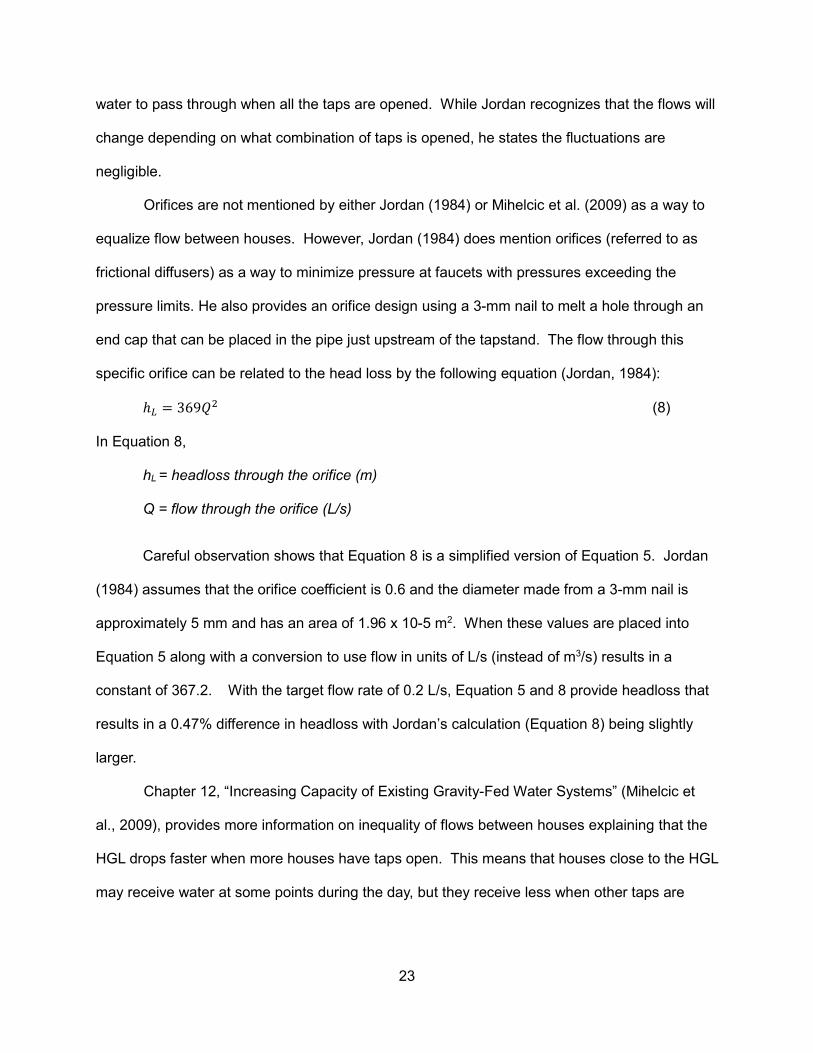
Orifices are not mentioned by either Jordan (1984) or Mihelcic et al. (2009) as a way to
equalize flow between houses. However, Jordan (1984) does mention orifices (referred to as
frictional diffusers) as a way to minimize pressure at faucets with pressures exceeding the
pressure limits. He also provides an orifice design using a 3-mm nail to melt a hole through an
end cap that can be placed in the pipe just upstream of the tapstand. The flow through this
specific orifice can be related to the head loss by the following equation (Jordan, 1984):
ℎ� = 369< (8)
In Equation 8,
hL = headloss through the orifice (m) Q = flow through the orifice (L/s)
Careful observation shows that Equation 8 is a simplified version of Equation 5. Jordan
(1984) assumes that the orifice coefficient is 0.6 and the diameter made from a 3-mm nail is
approximately 5 mm and has an area of 1.96 x 10⁻⁵ m2. When these values are placed into
Equation 5 along with a conversion to use flow in units of L/s (instead of m3/s) results in a
constant of 367.2. With the target flow rate of 0.2 L/s, Equation 5 and 8 provide headloss that
results in a 0.47% difference in headloss with Jordan’s calculation (Equation 8) being slightly
larger.
Chapter 12, “Increasing Capacity of Existing Gravity-Fed Water Systems” (Mihelcic et
al., 2009), provides more information on inequality of flows between houses explaining that the
HGL drops faster when more houses have taps open. This means that houses close to the HGL
may receive water at some points during the day, but they receive less when other taps are
24
opens and sometimes no water at all. It also suggests the use of globe valves, to limit the flows
to the houses farther from the HGL. However, that chapter does not provide detailed
information in the determination of where or how to correctly limit these flows, but states that
“case-by-case examination of each system must be made for the proper installation of valves”
(Mihelcic et al, 2009).
Both Jordan (1984) and Mihelcic et al. (2009) rely on the HGL in the design of the
distribution network of a gravity flow water system. From the HGL, one can determine pipe
sizes to ensure adequate pressures throughout the entire network as well as avoiding negative
pressure regions. The maximum pressure depends on the type of pipe. In Panama, most
systems are constructed out of PVC, which has a maximum pressure limit of 100-m of head
(Mihelcic et al., 2009). More importantly, the HGL will provide the pressure at each tapstand.
This ensures that there is a reasonable amount of pressure for the user, while preventing
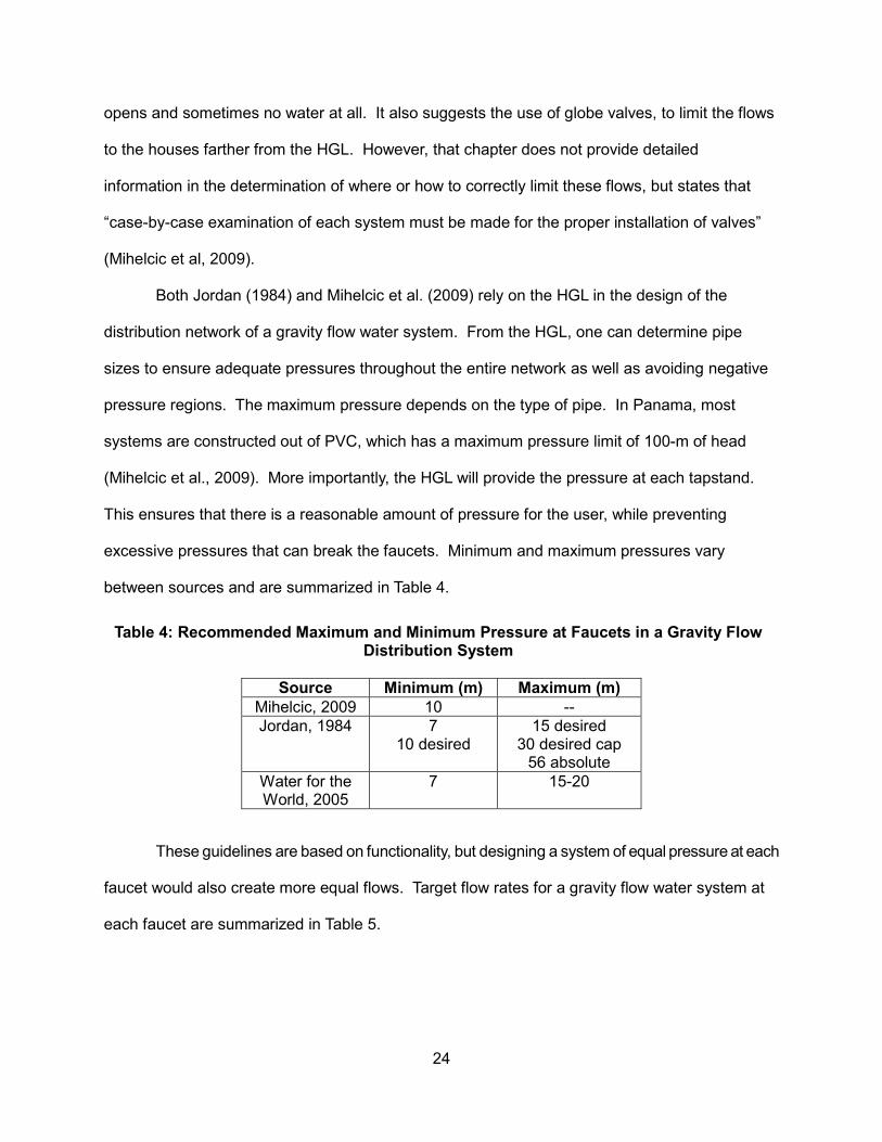
excessive pressures that can break the faucets. Minimum and maximum pressures vary
between sources and are summarized in Table 4.
Table 4: Recommended Maximum and Minimum Pressure at Faucets in a Gravity Flow Distribution System
These guidelines are based on functionality, but designing a system of equal pressure at each
faucet would also create more equal flows. Target flow rates for a gravity flow water system at
each faucet are summarized in Table 5.
Source Minimum (m) Maximum (m)
Mihelcic, 2009 10 -- Jordan, 1984 7
10 desired 15 desired
30 desired cap 56 absolute
Water for the World, 2005
7 15-20

25
Table 5: Recommended Maximum and Minimum Flow Rates at Faucets in a Gravity Flow Distribution System
Source Flow Rates (L/s)
NeatWork 0.1 Minimum 0.2 Desired
0.3 Maximum Jordan, 1984 0.2 minimum
0.225 desired Water for the World, 2005
0.03 minimum 0.23 maximum
Another important consideration of aqueduct design, is designing for the future so that
the aqueduct continues to function. As mentioned previously, normally the design life of a
gravity flow water system is assumed to be 20-25 years (Jordan, 1984). While both Jordan
(1984) and Mihelcic et al. (2009) mention this and determine required flows based on the design
population using a future population calculated using Equation 9 for populations under 2,000
people (Mihelcic et al., 2009), neither details how to adjust the design of the system for future
expansions.
=> = =? ∗ �1 + +×>&��� (9)
In Equation 9,
PN = the future population
P0 = the current population
r = rate of growth
N = number of years
Focusing on the future water requirement does not pose a problem to the users if they
are using communal taps and the additional population stays fairly centralized. However, it may
create a problem if faucets are added. Jordan (1984) suggests that the designer of the original
system can predict where future faucets may be added, design accordingly, and leave
instructions on where future faucets should be located. In Panama, where most systems
26
provide piped water directly to the individual houses it is not feasible to expect an author to
determine locations of all connections during the original design phase.
Suzuki (2010) assessed 28 water systems in Panama that Peace Corps Volunteers had
worked on. Of these, 17 were brand new systems and 11 were repaired. While he assessed
numerous characteristics, the relevant one for the research in this thesis is the distribution line.
Suzuki recognized there was inequality in flow between houses with those at a higher elevation
and farther away from the tank receiving less water, and this problem was made worse when
additional household connections were added to the system without proper design. He also
observed that the houses with leaky taps from excess pressure have little incentive to repair the
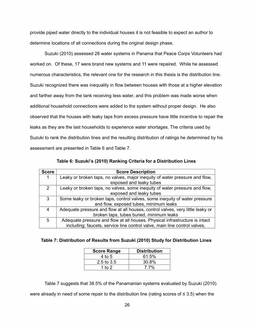
leaks as they are the last households to experience water shortages. The criteria used by
Suzuki to rank the distribution lines and the resulting distribution of ratings he determined by his
assessment are presented in Table 6 and Table 7.
Table 6: Suzuki’s (2010) Ranking Criteria for a Distribution Lines
Score Score Description
1 Leaky or broken taps, no valves, major inequity of water pressure and flow, exposed and leaky tubes
2 Leaky or broken taps, no valves, some inequity of water pressure and flow, exposed and leaky tubes
3 Some leaky or broken taps, control valves, some inequity of water pressure and flow, exposed tubes, minimum leaks
4 Adequate pressure and flow at all houses, control valves, very little leaky or broken taps, tubes buried, minimum leaks
5 Adequate pressure and flow at all houses. Physical infrastructure is intact including; faucets, service line control valve, main line control valves,
Table 7: Distribution of Results from Suzuki (2010) Study for Distribution Lines
Score Range Distribution
4 to 5 61.5% 2.5 to 3.5 30.8%
1 to 2 7.7%
Table 7 suggests that 38.5% of the Panamanian systems evaluated by Suzuki (2010)
were already in need of some repair to the distribution line (rating scores of ≤ 3.5) when the
27
average system is only 4 years old. This means it is necessary to provide a water committee
with more maintenance training and materials (Suzuki found that few communities possessed
any sort of operator’s manual) or the communities will need more outside assistance possibly in
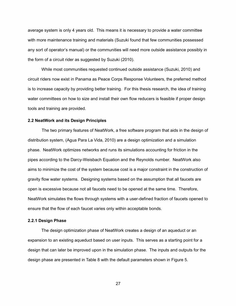
the form of a circuit rider as suggested by Suzuki (2010).
While most communities requested continued outside assistance (Suzuki, 2010) and
circuit riders now exist in Panama as Peace Corps Response Volunteers, the preferred method
is to increase capacity by providing better training. For this thesis research, the idea of training
water committees on how to size and install their own flow reducers is feasible if proper design
tools and training are provided.
2.2 NeatWork and its Design Principles
The two primary features of NeatWork, a free software program that aids in the design of
distribution system, (Agua Para La Vida, 2010) are a design optimization and a simulation
phase. NeatWork optimizes networks and runs its simulations accounting for friction in the
pipes according to the Darcy-Weisbach Equation and the Reynolds number. NeatWork also
aims to minimize the cost of the system because cost is a major constraint in the construction of
gravity flow water systems. Designing systems based on the assumption that all faucets are
open is excessive because not all faucets need to be opened at the same time. Therefore,
NeatWork simulates the flows through systems with a user-defined fraction of faucets opened to
ensure that the flow of each faucet varies only within acceptable bonds.
2.2.1 Design Phase
The design optimization phase of NeatWork creates a design of an aqueduct or an
expansion to an existing aqueduct based on user inputs. This serves as a starting point for a
design that can later be improved upon in the simulation phase. The inputs and outputs for the
design phase are presented in Table 8 with the default parameters shown in Figure 5.

28
Table 8: Input and Output for NeatWork’s Design Phase
Inputs Outputs
Node List: ID, height, X and Y coordinates1, number of faucets, and
nature (i.e., tank, node, or tap)
Ideal orifice size
Arc List: Begin ID, End ID, and Length Commercial orifice size Types of pipes that can be used Diameter of pipe2
Constraints on pipe sizes for specific arcs Orifice diameters that can be installed
Parameters Modified Load Factors
1 The X and Y coordinates can be used for advanced features. If there is no plan to use these features, entering 0 for all of them does not affect the design.
2 Sometimes a segment will be broken into two different diameters. In these cases, the lengths of each segment are provided as well.
Figure 5: Screenshot of NeatWork's Design Parameter Input Section That Shows Required Inputs and Default Values
NeatWork uses the service quality input (Figure 5) to determine the flow through each
pipe segment during design. The higher the service quality, the greater the flows through each
branch will be resulting in a more reliable, but more expensive system. The service quality is
based on conditional and cumulative probabilities of how many faucets will receive water

29
through that pipe segment. φ (L/s) represents the flow through the pipe needed for one faucet
to have sufficient water. For each additional faucet added, φ is multiplied by the number of
faucets to determine the flow through the pipe if that number of faucets were open. If the pipe
leads to one faucet, the flow through that pipe will be φ L/s. If a pipe leads to six faucets, the
flow will be between φ and 6φ depending on the number of faucets open. Because at least one
faucet needs to be opened for a flow to exist through the pipe, the conditional probabilities can
be calculated as follows (Agua Para La Vida, 2010):
P(B, A) =+H∗(&I+)JK�∗ L!
H!∗(JKH)!&I(&I+)J (10)
In Equation 10,
r = probability that a faucet is open (defined as fraction of open faucets in NeatWork
input)
N = total number of faucets
n = number of faucets open for trial
Using Equation 10, the flows and conditional and cumulative probabilities for the
different combinations of open and closed faucets can be calculated for each pipe segment.
An example of these probabilities for a pipe that leads to six faucets are presented in Table 9.
The service quality is equivalent to the cumulative probability. If the user selects a
service quality of 0.5220, the system will design the pipes based on a flow of 2φ (the flow
required to provide 2 taps with water) and that will be great enough to cover the demand flow
52.20% of the time. When the service quality falls between the cumulative probabilities for the
flows, the flow is linearly interpolated and this becomes the suggested load factor. The user has
the ability to enter modified load factors for each pipe segment.

30
Table 9: Flows and Probabilities Used in the Calculation of the Service Quality Factor in NeatWork
Open Faucets
1 2 3 4 5 6
Flow (L/s) Φ 2φ 3φ 4φ 5φ 6φ Conditional Probability
0.1958 0.3263 0.2900 0.1450 0.0387 0.0043
Cumulative Probability
0.1958 0.5220 0.8120 0.9570 0.9957 1
Another unique aspect of NeatWork is that it designs under the assumption that the
consumers need practically no water pressure at the faucets. While pressure may not be
needed, it minimizes the factor of safety that may be required due to errors in survey data.
However, NeatWork does incorporate a factor of safety in the way it calculates the roughness
factor of the pipes. Over time calcium deposits builds up in pipes in some locations of the
distribution system and sediments in a PVC pipe of a gravity flow water system can result in
higher frictional losses. NeatWork incorporates this into its calculations and uses a friction
factor 4.5% greater than that of a smooth PVC pipe (Agua Para La Vida, 2010).
Along with using pipe sizes to obtain the desired headloss at each faucet, NeatWork
also relies on flow reducers. The headloss through an orifice depends on the Reynolds number
if the hole diameter exceeds 30% of the pipe diameter. The sizes of perforations used by
NeatWork are almost always smaller than this. Therefore, the program calculates headloss
based solely on flow rate and hole diameter as follows (Agua Para La Vida, 2010):
ℎ� = −OP Q�
R� (11)
In Equation 11,
hL = headloss through the orifice (m)
Ѳ = orifice coefficient (unitless)
Q = flow through the orifice (m3/s)
d = diameter of hole in orifice (m)

31
While the orifice coefficient (Ѳ) can be changed by the designer, NeatWork uses a
default value of 0.59. Since the manual was written more tests have been conducted
suggesting that a better estimate for Ѳ is 0.62 (personal communication with Guillermo Corcos,
2015). This produces headloss values 35% smaller than Equation 5. The varying headloss for
the target flow of 0.2 L/s is presented in Table 10.
Table 10: Comparing Headloss Values through Orifices
Diameter (m)
NeatWork Formula
(m)
Equation 5 (m)
0.003 73.0 113.3
0.004 23.1 35.9
0.005 9.5 14.7
0.006 4.6 7.1
Guillermo Corcos, the technical director for Agua Para la Vida, has performed a variety
of tests systematically varying pressure loss, flows, and orifice diameter in order to test the
NeatWork formula (Equation 11) and determined that the simplified NeatWork formula was
acceptable to use for gravity flow aqueducts. Because the NeatWork formula was derived
specifically for this application while Equation 5 is applied when using orifices to measure flows,
this thesis proceeds using the NeatWork formula.
2.2.2 Simulation Phase
The simulation phase allows the designer to test the designs created by NeatWork or
existing aqueduct designs that were constructed in the past. To start a simulation, the user can
define variables in a pop-up window as shown in Figure 6. The values shown in Figure 6 are
the default values provided by NeatWork.

32
Figure 6: Screenshot of Simulation Parameter Inputs in NeatWork
The NeatWork simulation will produce various results including the velocities through
pipes, the node pressures, and a variety of information regarding the flow at faucets including:
1) faucet ID, 2) number of occurrences, 3) minimum flow 4) average flow, 5) maximum flow, 6)
variability, 7) percentage below the lower bound, 8) percentage above the upper bound, and 9)
number of failures. The user can then manipulate pipe sizes and change flow reducer sizes to
improve the functionality of the system until the user believes that the level of service will meet
the community needs.
NeatWork assumes that the storage tank will also have plenty of water. If the tank
empties at some points during the day, the taps will have water less frequently than predicted by
the NeatWork model. Measurements of dry season flows and calculations of water needs
should therefore be performed to verify that there is sufficient water. This is essential for the
sustainability of an aqueduct. For the purpose of this thesis, the author assumes there is
always a sufficient amount of water in the storage tank so that the NeatWork analyses are
accurate.

33
Chapter 3: Materials and Methods
3.1 Making a Water Level
Water levels are basic tools used to measure the change in elevations along an
aqueduct. They can be made using two ½-inch PVC pipes or straight narrow sticks cut to be
about 6-ft tall (the author’s was 80-inches in length) and ¼-inch vinyl tubing about 32-ft long as
seen in Figure 7.
Figure 7: A Completed Water Level
Using a tape measure and a permanent marker, the pipes are marked every inch or
centimeter. The author used a water level marked in inches and converted the data to
centimeters to use in NeatWork. For future water levels, it is recommended to mark everything
in centimeters to eliminate this conversion. Using zip ties or duct tape, the tubing is attached
about 5-inches from the bottom of the PVC pipes so that when the vinyl tubing is fully extended

34
the pipes are 20-ft or 6-m apart. The tubing is continually attached to the top of the PVC pipes
making sure not to cover any of the numbers. The tubing should be securely attached to the
PVC pipes without pinching the tube preventing water from passing. The vinyl tubing is then
filled with water so that the water reaches halfway up the PVC pipes. It is important to make
sure all air bubbles are removed. This can be accomplished by raising the elevation of the tube
close to the air bubble and gently tapping below the bubble.
3.2 Data Collection and Organization
During the time the author served as a Peace Corps Volunteer, she surveyed the
existing aqueduct in need of a new distribution network with the help of community members
using a water level made as described above. A team cleared the path of the pipes with
machetes so the author and her team of two helpers could survey.
Starting at the source and following the pipe, the author surveyed the entire system
including all main lines and the individual branches leading to each house. While some houses
have multiple faucets, the author only surveyed to the faucet used the most. The helpers would
extend the water level to its maximum distance and would read off the closest number to the
level of the water, which the author would record. The leading person would mark the spot of
the water level so the follower could put their tube in the same spot and the process would be
repeated. At crucial spots such as tees, changes in pipe sizes, and high and low points, the
lead person would place his pipe at the crucial spot and the distance between the two pipes
would be measured. GPS coordinates were also taken at all the crucial points. If the slope was
too steep where the change in elevation was greater than what could be measured by the water
level, readings would be recorded for two points closer together and their horizontal distance
would be measured. After the existing aqueduct was surveyed, the additional houses that
wanted to be added to the system were surveyed as well from the closest known point of the
existing aqueduct.
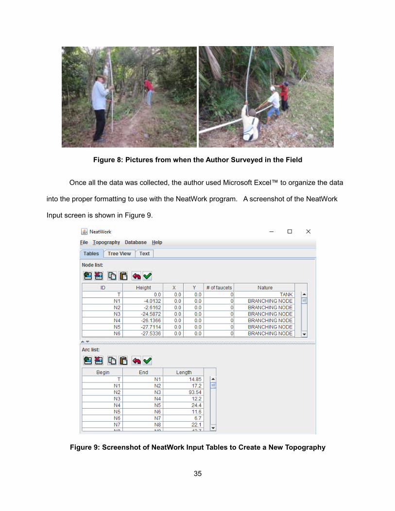
35
Figure 8: Pictures from when the Author Surveyed in the Field
Once all the data was collected, the author used Microsoft Excel™ to organize the data
into the proper formatting to use with the NeatWork program. A screenshot of the NeatWork
Input screen is shown in Figure 9.
Figure 9: Screenshot of NeatWork Input Tables to Create a New Topography

36
NeatWork performs faster with fewer data points so the author simplified the data to
include only critical points including the tank, high points, low points, tees, and faucets to use as
nodes. She calculated the relative altitude for each node, setting the tank as the benchmark at
an elevation of 0-m. She also calculated the distance between each node. NeatWork has
additional columns that allow the user to enter horizontal coordinates that may be helpful when
designing loop systems. However, NeatWork itself does not use these coordinates during the
design (Agua Para La Vida, 2010). Using the coordinate features provided no advantages since
the Santa Cruz system contains no loops. Therefore, 0 was inputted for the X and Y
coordinates. The tank and all branching nodes have 0 faucets while all houses were assumed
to have 1 faucet to simplify the aqueduct design. The following numbers were assigned for the
nature of each node: tank-0, branching node-1, and faucet-2. The author modified the Excel
document and copied and pasted the tables into Neatwork to create the various topography files
she needed to perform the analysis of the aqueduct.
3.3 Procedure for Analyzing Sample Aqueduct
The author utilizes NeatWork as the primary tool for analyzing the system. For the
purpose of this research she used its default values for running simulations. She also assumed
that a water committee is trained on how to repair leaks in the system and will repair them on a
regular basis so friction losses associated with broken pipes can be ignored during the analysis.
As explained in Section 1.7, the aqueduct used for this research has 60 confirmed
connections and 13 potential connections. All 73 connections were surveyed for this study
allowing them to be analyzed using the NeatWork software. In order to better analyze how the
addition of these 13 houses would affect performance of the aqueduct a variety of different
simulations were run in NeatWork.
The designs come from two topographies; “All” which includes all 73 houses and “As Is”
which only contains the 60 confirmed connections. The Excel tables copied into NeatWork are

37
reproduced in Appendix B. From both of the topography files, NeatWork produced designs
utilizing only the pipes and flow reducers as presented in Table 11.
Table 11: Design Input Criteria for Design of Sample Aqueduct
Pipe Size
Flow Reducer Diameter
Nominal Diameter
(in)
Standard Dimension
Ratio (SDR)
(m) (in)
0.5 13.5 0.002381 3/32
1 26.0 0.003175 1/8
1.5 26.0 0.003969 5/32
2 26.0 0.004763 3/16
3 26.0 0.005556 7/32 0.006350 1/4
These pipe sizes were selected based on local availability, necessary strength, and cost.
The pipe sizes listed in Table 11 are also available in Standard Dimension Ratio (SDR) 41, but
these are not recommended for use in gravity flow water systems because of their low pressure
ratings. In some stores in Penenomé, the city closest to Santa Cruz with hardware stores, 2.5-
inch PVC pipe could be specially purchased making it more expensive. Other stores also
carried 1.25-inch PVC, but at almost the same price as the 1.5-inch pipe. Therefore, the 1.25-
inch and 2.5-inch pipes were left out of the design. This also reduces the number of extra pipes
a water committee needs to have locally available to repair damaged pipes.
The holes for the flow reducers are created using hand drills which were only available in
Panama in inches. Therefore, the standard drill bit sizes in inches were converted to meters,
the unit used in NeatWork, so that the edited orifice database in NeatWork reflects the available
sizes.
Occasionally, the NeatWork design provided a 1-inch pipe leading directly to a tapstand
which makes it more difficult in the field to connect the tapstand and install the flow reducer.

38
Therefore, the author modified the design in Neatwork to include 6-m (the standard pipe length)
of ½-inch PVC pipe before every faucet where this occurred. The designs were then saved as
“All” and “As Is” in Neatwork. A simulation was run on both of the designs using the NeatWork
values. Both designs were compared to each other noting the pipe sections and flow reducer
diameters that changed from the addition of the 13 unconfirmed houses.
If the 13 unconfirmed houses represent houses being added to the system in the future,
it is more likely that they were not included in the original design. Therefore, another design file
was created in NeatWork using the “All Topography”; however, pipe size constraints were input
to match the pipe sizes from the “As Is” design file pipe sizes. After NeatWork provides an initial
design, the flow reducer sizes must be manually changed to match those from the “As Is”
design file for the existing houses because a limitation of NeatWork is that is does not allow the
designer to specify the size of flow reducers prior to a design. This design was saved as “All As
Is Sizes” and a simulation using the default values was run on this design. This file represents
the correct flow reducer sizes according to NeatWork.
However, without the use of NeatWork, most communities will not be able to install the
appropriate sized flow reducer. Therefore, the flow reducer sizes were modified in the “All As Is
Sizes” design to reflect different scenarios and saved as different design files: if no flow
reducers are installed- “All As Is Sizes No Discs, if the most common flow reducer size of 5/32-
inch is installed for all new houses- “All As Is Sizes Discs 396,” and if the flow reducer is sized
based on the flow reducer size of the closest house- “All As Is Discs Closest.” The flow reducer
sizes used when sized based on the closest house are provided in Table 12.
The descriptions from the preceding six design files are summarized in Table 13. The
results from the different NeatWork simulation were compared to evaluate the differences in
service quality between the designs.
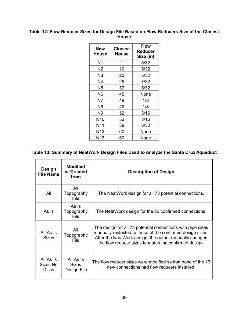
39
Table 12: Flow Reducer Sizes for Design File Based on Flow Reducers Size of the Closest House
New House
Closest House
Flow Reducer Size (in)
N1 1 5/32
N2 19 5/32
N3 20 5/32
N4 25 7/32
N5 37 5/32
N6 45 None
N7 49 1/8
N8 49 1/8
N9 52 3/16
N10 52 3/16
N11 58 5/32
N12 60 None
N13 60 None
Table 13: Summary of NeatWork Design Files Used to Analyze the Santa Cruz Aqueduct
Design File Name
Modified or Created
from Description of Design
All All
Topography File
The NeatWork design for all 73 potential connections.
As Is As Is
Topography File
The NeatWork design for the 60 confirmed connections.
All As Is Sizes
All Topography
File
The design for all 73 potential connections with pipe sizes manually restricted to those of the confirmed design sizes. After the NeatWork design, the author manually changed
the flow reducer sizes to match the confirmed design.
All As Is Sizes No
Discs
All As Is Sizes
Design File
The flow reducer sizes were modified so that none of the 13 new connections had flow reducers installed.

40
Table 13: (Continued)
All As Is Sizes
Discs 396
All As Is Sizes
Design file
The flow reducer sizes were modified so that all 13 of the new connections would have a flow reducer sized at 5/32-
inch.
All As Is Sizes Discs
Closest
All As Is Sizes De-sign File
The flow reducer sizes were modified so that the 13 new connections have a flow reducer equal to that of the closest
confirmed house on the system.
Along with the NeatWork analysis of varying designs, the author examined the system
looking for patterns and ways to simply flow reducer sizes in order to create a tool appropriate
for local water committees. This procedure was more experimental where the author based her
procedures on her findings as she went.
First, the different flow reducer sizes, relative altitudes, and total distances from the tank
for each faucet were compared. These values come from the original surveying data. Next, the
author determined different pressures at each node based on the “All As Is Sizes”. NeatWork
provided an average pressure and a maximum pressure that occurred at each node during the
simulation. Available head was calculated using traditional fluid mechanics as well. Using the
average flow between each node provided by the NeatWork simulation, the author used
Equation 2 to calculate a friction factor and Equation 1 to calculate a headloss for each segment
of pipe. A cumulative headloss leading to each node was summed and converted to available
head by subtracting the total headloss form the distance in elevation between the tank and the
node. Appendix E shows the spreadsheet used to calculate the available head. The ranges for
average pressure, maximum pressure, and available head were determined for each flow
reducer size.
Next, the author examined how the size of the flow reducer determined by NeatWork in
the “All As Is Design” compared to the flow reducer size installed in the closest house and noted

41
the locations where they differed. To better understand these locations, the author created
profiles of these from her surveying data. She then identified other areas of the aqueduct that
did not have new houses that would have similar profiles and plotted these as well. The author
summarized the trends in three different rules that could be used to size flow reducers without
the use of NeatWork.
3.4 Testing Rules from Analysis
In order to test the rules made from the analysis explained in detail in Section 4.1, the
author added experimental houses where additional houses may be built in the future. Since
the actual aqueduct that was built for the community of Santa Cruz was designed from the
Neatwork design for all the houses, the “All” design file was used as the basis for sizing the flow
reducers of the experiment houses. The author selected 9 locations that are shown in Figure
10.
Initially, the author created a new topography file called “Experiments” that included all 9
of the experiment houses. Using this file and inputting the sizes of the pipes from the “All”
design file, a new design was created entitled “Experiments All Sizes.” However, because
NeatWork does not allow the user to input flow reducer sizes before the design, it changed the
flow reducer sizes on 25 houses including most of them on the branches that had experiment
houses added to it. This is drastically different from when this same technique was performed
to create the “All As Is Sizes” design that only resulted in a change of three flow reducer sizes.
This difference is believed to be a result from the fact that in the “Experiments” topography all
the additional houses were placed at the end of the branches when in the “All” topography the
new houses were spread randomly throughout the system. With the large number of changes
in flow reducers, the sizes given to the new houses do not accurately represent the sizes that
those houses should have if it was individually added to the aqueduct.

42
Figure 10: Map Including Experiment Houses to Test Developed Rules for Sizing Flow Reducers Showing Flow Reducer Sizes and Faucet Numbers from “All” Design (not to
scale)
To fix this problem and get more accurate flow reducer sizes, nine new topography files
were created named “X1” to “X9” where each one only had the addition of one experimental
house. Design files, “X1 All Sizes” - “X9 All Sizes”, were then created using these nine
topographies and manually inputting the pipe sizes from the “All” design file. While the majority
of the flow reducer sizes stayed the same, in many of the trials, the flow reducer sizes of nearby
houses changed. The NeatWork sized flow reducer still may not necessarily represent the ideal
size for the new house because the end branches are sensitive to new houses and some flow
reducer sizes changed. While changing the flow reducers in other surrounding houses might
create a more optimal aqueduct, this would be more complicated for the water committee.
Therefore, this thesis assumes that all existing flow reducers will remain the same size and
were changed to match the initial size from the “All” design file. If the NeatWork sized flow
reducer varied from the flow reducer size predicted from the author’s conclusions, the flow

43
reducer for the new experimental house was changed and saved as a new design file, such as
“X1 All Sizes PS” where PS stands for predicted size. For further comparison, additional design
files were made to test how the system would operate if the flow reducer was installed to match
that of the closest house. The flow reducers for the new experiment houses were changed and
saved with a “CH” at the end of the file name for closest house. The author ran NeatWork
simulations on all of these design files to determine which flow reducer sizes optimized
aqueduct performance.

44
Chapter 4: Results and Discussion
4.1 Analysis of Sample Aqueduct
The results of the simulations on the various designs were analyzed. When NeatWork
created designs, the majority of the pipe sizes and flow reducers were the same. However,
there were some differences in estimated pipe size. The complete distribution system for the
“All” design file for 73 houses consists of 4,284-m of pipe. 650-m of this total pipe length
increased in diameter when the design included the entire system of 73 houses compared to
only the 60 confirmed houses. This means that 13.5% of the pipe diameter dimensioning
should be changed when the number of system users is increased from 60 to 73 (22%). This is
because as more houses are added to the system the flow through the pipes becomes larger to
meet increased demand of the community. As flows increase, headloss through the pipe also
increases, which makes it more difficult for the water to arrive at the higher elevation homes and
those homes farther from the storage tank. To prevent additional headloss, larger diameter
pipes can be added as the bigger pipes create less headloss. The specific places where the
pipe sizes are different identified from NeatWork simulations are presented in Table 14 and the
summary of the lengths of pipe sizes that would require changing under this scenario is
provided in Table 15.
While 13.5% of the pipes increased in diameter when the 13 additional houses were
added, only 3 of 60 (5%) of the confirmed houses required a change in flow reducer size. The
differences in flow reducer sizes are shown in Table 16 and their locations in the aqueduct are
presented in Figure 11.
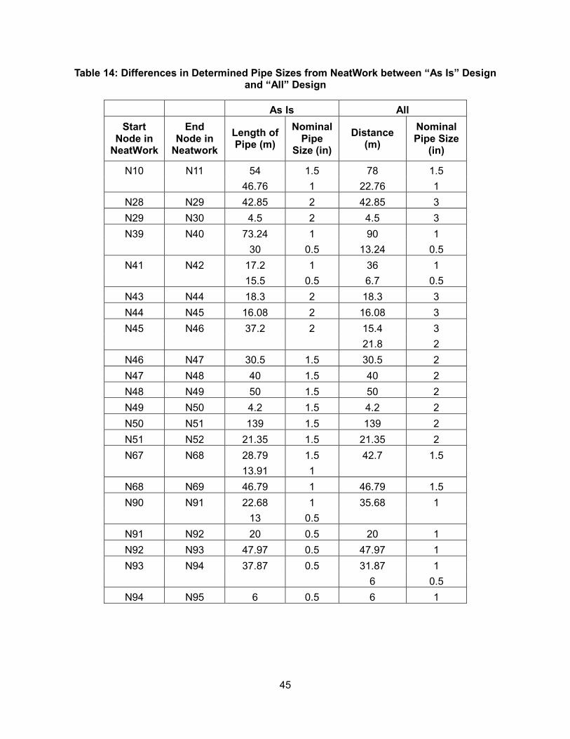
45
Table 14: Differences in Determined Pipe Sizes from NeatWork between “As Is” Design and “All” Design
As Is All
Start Node in
NeatWork
End Node in
Neatwork
Length of Pipe (m)
Nominal Pipe
Size (in)
Distance (m)
Nominal Pipe Size
(in)
N10 N11 54 1.5 78 1.5
46.76 1 22.76 1
N28 N29 42.85 2 42.85 3
N29 N30 4.5 2 4.5 3
N39 N40 73.24 1 90 1
30 0.5 13.24 0.5
N41 N42 17.2 1 36 1
15.5 0.5 6.7 0.5
N43 N44 18.3 2 18.3 3
N44 N45 16.08 2 16.08 3
N45 N46 37.2 2 15.4 3
21.8 2
N46 N47 30.5 1.5 30.5 2
N47 N48 40 1.5 40 2
N48 N49 50 1.5 50 2
N49 N50 4.2 1.5 4.2 2
N50 N51 139 1.5 139 2
N51 N52 21.35 1.5 21.35 2
N67 N68 28.79 1.5 42.7 1.5
13.91 1
N68 N69 46.79 1 46.79 1.5
N90 N91 22.68 1 35.68 1
13 0.5
N91 N92 20 0.5 20 1
N92 N93 47.97 0.5 47.97 1
N93 N94 37.87 0.5 31.87 1
6 0.5
N94 N95 6 0.5 6 1

46
Table 15: Total Length of Pipes Changed between “As Is” Design and “All” Design
Pipe Size Change (in)
Length of Pipe Requiring
Change (m)
2 to 3 97
1.5 to 2 285
1 to 1.5 114
0.5 to 1 154
Figure 11: Location of Faucets as Indicated in the Red Circles where the Flow Reducer Size Changes when the Design Changes from the “As Is” Design to the “All” Design (not
to scale)

47
Table 16: Differences in Flow Reducer Sizes between “As Is” Design and “All” Design
Flow Reducer Size (in)
House From “As Is” Design
From “All” Design
21 0.003969 0.004763
51 -- 0.006350
60 -- 0.006350
NeatWork simulations performed with the default values listed in Figure 6 were run on
the six designs summarized in Table 13. Appendix C presents the complete design results
including number of occurrences that a faucet was used in a simulation, minimum flow, average
flow, maximum flow, variability of flows, percentage of time flow is less than 0.1 L/s, and
percentage of times flow is greater than 0.3 L/s. While the flows changed in all the connections,
a notable change is defined as if in one of the simulations a new no flow (0.0 L/s minimum flow)
or that the flow is below 0.1 L/s more than 25% of the time. The notable changes in flows
between the designs are summarized in Table 17.
Table 17: Notable Changes between Designs for Sample Aqueduct in Minimum Flow and Percentage of Time Below 0.1 L/s
As Is All All As Is
Sizes
All As Is Sizes No
Discs
All As Is Sizes Discs
396
All As Is Sizes Discs
Closest
House min (L/s)
<0.1 L/s (%)
min (L/s)
<0.1 L/s (%)
min (L/s)
<0.1 L/s (%)
min (L/s)
<0.1 L/s (%)
min (L/s)
<0.1 L/s (%)
min (L/s)
<0.1 L/s (%)
13 0.000 11.9 0.072 2.6 0.042 5.7 0.000 12.1 0.041 11.1 0.032 13.6
14 0.000 9.4 0.082 2.7 0.047 10.3 0.000 16.7 0.000 8.5 0.043 9.3
26 0.064 6.3 0.056 12.2 0.016 15.0 0.000 23.7 0.025 12.2 0.000 16.2
44 0.082 2.7 0.121 0.0 0.016 7.1 0.000 9.5 0.068 12.8 0.000 23.3
45 0.000 20.5 0.000 4.8 0.000 43.8 0.000 41.2 0.000 73.5 0.000 53.3
51 0.132 0.0 0.134 0.0 0.000 29.0 0.000 82.1 0.000 97.5 0.000 30.0
56 0.000 13.6 0.054 2.5 0.000 55.3 0.000 91.3 0.000 52.4 0.000 60.0
60 0.124 0.0 0.087 10.3 0.000 57.6 0.000 88.6 0.000 55.0 0.000 60.5
N6 -- -- 0.142 0.0 0.064 2.5 0.076 2.9 0.049 33.3 0.000 2.2
N12 -- -- 0.140 0.0 0.052 31.6 0.000 51.1 0.047 74.3 0.041 14.3
N13 -- -- 0.108 0.0 0.015 61.1 0.000 84.2 0.010 53.7 0.000 63.4
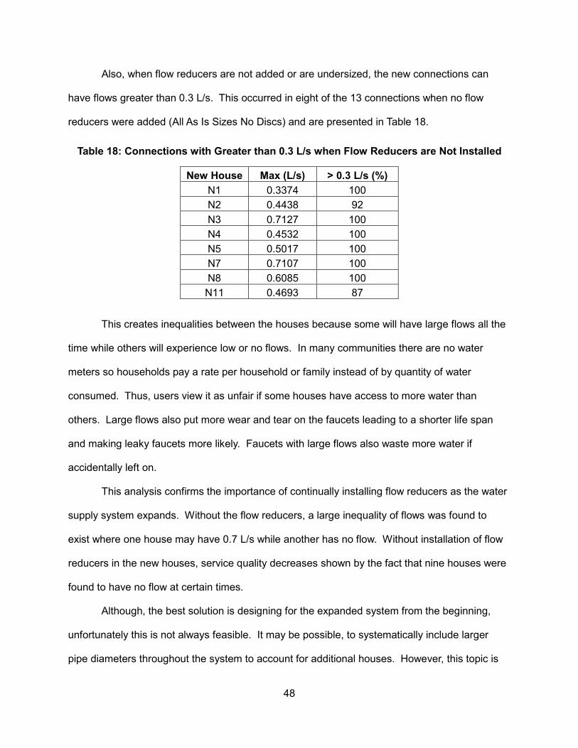
48
Also, when flow reducers are not added or are undersized, the new connections can
have flows greater than 0.3 L/s. This occurred in eight of the 13 connections when no flow
reducers were added (All As Is Sizes No Discs) and are presented in Table 18.
Table 18: Connections with Greater than 0.3 L/s when Flow Reducers are Not Installed
New House Max (L/s) > 0.3 L/s (%)
N1 0.3374 100
N2 0.4438 92
N3 0.7127 100
N4 0.4532 100
N5 0.5017 100
N7 0.7107 100
N8 0.6085 100
N11 0.4693 87
This creates inequalities between the houses because some will have large flows all the
time while others will experience low or no flows. In many communities there are no water
meters so households pay a rate per household or family instead of by quantity of water
consumed. Thus, users view it as unfair if some houses have access to more water than
others. Large flows also put more wear and tear on the faucets leading to a shorter life span
and making leaky faucets more likely. Faucets with large flows also waste more water if
accidentally left on.
This analysis confirms the importance of continually installing flow reducers as the water
supply system expands. Without the flow reducers, a large inequality of flows was found to
exist where one house may have 0.7 L/s while another has no flow. Without installation of flow
reducers in the new houses, service quality decreases shown by the fact that nine houses were
found to have no flow at certain times.
Although, the best solution is designing for the expanded system from the beginning,
unfortunately this is not always feasible. It may be possible, to systematically include larger
pipe diameters throughout the system to account for additional houses. However, this topic is
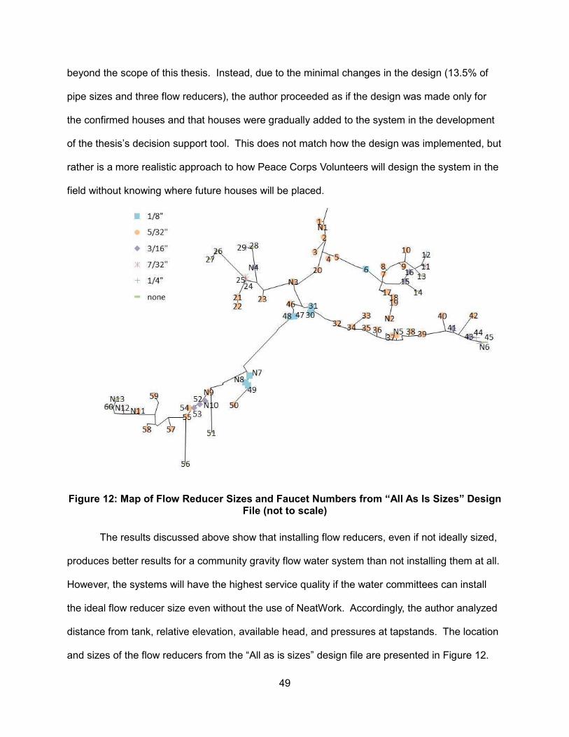
49
beyond the scope of this thesis. Instead, due to the minimal changes in the design (13.5% of
pipe sizes and three flow reducers), the author proceeded as if the design was made only for
the confirmed houses and that houses were gradually added to the system in the development
of the thesis’s decision support tool. This does not match how the design was implemented, but
rather is a more realistic approach to how Peace Corps Volunteers will design the system in the
field without knowing where future houses will be placed.
Figure 12: Map of Flow Reducer Sizes and Faucet Numbers from “All As Is Sizes” Design File (not to scale)
The results discussed above show that installing flow reducers, even if not ideally sized,
produces better results for a community gravity flow water system than not installing them at all.
However, the systems will have the highest service quality if the water committees can install
the ideal flow reducer size even without the use of NeatWork. Accordingly, the author analyzed
distance from tank, relative elevation, available head, and pressures at tapstands. The location
and sizes of the flow reducers from the “All as is sizes” design file are presented in Figure 12.

50
This information is also presented in Table 19 with the relative altitude using the tank as the
benchmark.
Table 19: Flow Reducer Sizes, Relative Altitudes, Length of Pipes between Tank and Faucet for Santa Cruz Aqueduct, Available Head, Average Pressure, and Maximum
Pressure
House
Flow Re-
ducer Size (in)
Rela-tive
Altitude (m)
Length of Pipes Between Tank and
Faucet (m)
House
Flow Re-
ducer Size (in)
Rela-tive
Altitude (m)
Length of Pipes Between Tank and
Faucet (m)
1 5/32 -27.8 145 38 5/32 -22.4 840
2 5/32 -29.3 172 39 5/32 -35.3 842
3 5/32 -32.9 319 40 5/32 -36.8 960
4 5/32 -32.4 264 41 3/16 -33.7 946
5 5/32 -36.1 272 42 5/32 -39.0 1033
6 1/8 -46.4 383 43 3/16 -31.9 1004
7 5/32 -46.1 445 44 1/4 -25.2 1016
8 5/32 -43.9 468 45 none -22.2 1091
9 5/32 -34.6 510 46 5/32 -47.4 468
10 5/32 -35.5 549 47 1/8 -48.3 501
11 7/32 -26.0 575 48 1/8 -48.4 501
12 1/4 -23.2 600 49 1/8 -49.3 763
13 none -20.9 585 50 5/32 -40.5 839
14 none -20.1 566 51 none -17.1 879
15 3/16 -31.1 514 52 3/16 -25.4 884
16 3/16 -29.5 538 53 3/16 -26.5 900
17 5/32 -44.8 472 54 5/32 -31.3 917
18 5/32 -45.9 505 55 5/32 -30.8 935
19 5/32 -46.0 502 56 none -15.5 1092
20 5/32 -27.9 249 57 5/32 -36.4 1053
21 5/32 -31.4 552 58 5/32 -42.2 1115
22 5/32 -35.5 585 59 5/32 -44.2 1137
23 5/32 -29.9 487 60 none -27.5 1233
24 3/16 -22.4 520 N1 5/32 -29.8 151
25 7/32 -23.1 557 N2 5/32 -47.7 542
26 none -17.3 629 N3 5/32 -35.9 316
27 none -19.1 664 N4 3/16 -23.8 535
28 none -18.0 612 N5 5/32 -30.2 785
29 1/4 -19.8 590 N6 1/4 -25.6 1075
30 1/8 -48.3 460 N7 1/8 -50.1 727
31 1/8 -48.6 455 N8 1/8 -49.8 757
32 5/32 -41.0 556 N9 5/32 -33.8 831
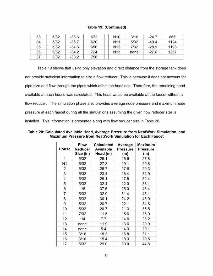
51
Table 19: (Continued)
33 5/32 -38.6 672 N10 3/16 -24.7 865
34 5/32 -36.7 620 N11 5/32 -40.4 1124
35 5/32 -34.6 656 N12 7/32 -28.9 1198
36 5/32 -34.2 724 N13 none -27.6 1257
37 5/32 -30.2 758
Table 19 shows that using only elevation and direct distance from the storage tank does
not provide sufficient information to size a flow reducer. This is because it does not account for
pipe size and flow through the pipes which affect the headloss. Therefore, the remaining head
available at each house was calculated. This head would be available at the faucet without a
flow reducer. The simulation phase also provides average node pressure and maximum node
pressure at each faucet during all the simulations assuming the given flow reducer size is
installed. This information is presented along with flow reducer size in Table 20.
Table 20: Calculated Available Head, Average Pressure from NeatWork Simulation, and Maximum Pressure from NeatWork Simulation for Each Faucet
House Flow
Reducer Size (in)
Calculated Available Head (m)
Average Pressure
(m)
Maximum Pressure
(m)
1 5/32 25.1 15.6 27.8
N1 5/32 27.3 19.1 29.8
2 5/32 26.7 17.6 29.3
3 5/32 23.4 18.4 32.9
4 5/32 28.1 17.5 32.4
5 5/32 32.4 22.0 36.1
6 1/8 37.6 25.0 46.4
7 5/32 32.9 31.4 46.1
8 5/32 30.1 24.2 43.9
9 5/32 20.7 22.1 34.6
10 5/32 20.7 21.3 35.5
11 7/32 11.5 15.6 26.0
12 1/4 7.7 14.6 23.2
13 none 11.9 13.6 20.9
14 none 5.4 14.3 20.1
15 3/16 18.3 16.8 31.1
16 3/16 15.4 18.3 29.5
17 5/32 29.0 30.0 44.8

52
Table 20: (Continued)
18 5/32 28.5 31.7 45.9
19 5/32 28.7 26.2 46.0
N2 5/32 28.6 33.9 47.7
20 5/32 25.0 15.9 27.9
N3 5/32 31.8 20.1 35.9
21 5/32 19.5 19.1 31.4
22 5/32 22.2 21.7 35.5
23 5/32 19.1 17.0 29.9
24 3/16 11.2 13.4 22.4
25 7/32 10.4 14.5 23.1
26 none 5.4 10.4 17.3
27 none 5.7 11.2 19.1
N4 3/16 12.9 14.3 23.8
28 none 5.1 11.0 18.0
29 1/4 7.7 12.9 19.8
30 1/8 40.0 30.0 48.3
31 1/8 40.9 28.7 48.6
32 5/32 31.5 23.8 41.0
33 5/32 25.1 24.7 38.6
34 5/32 26.2 23.9 36.7
35 5/32 23.2 20.8 34.6
36 5/32 21.7 20.2 34.2
37 5/32 17.4 16.6 30.2
N5 5/32 17.1 20.0 35.7
38 5/32 20.2 16.6 30.2
39 5/32 19.9 20.5 35.3
40 5/32 17.8 21.7 36.8
41 3/16 15.6 22.6 33.7
42 5/32 18.5 23.8 39.0
43 3/16 13.5 19.2 31.9
44 1/4 6.4 14.6 25.2
N6 1/4 7.2 15.4 25.6
45 none 3.9 11.5 22.2
46 5/32 29.5 26.1 47.5
47 1/8 39.6 23.7 48.3
48 1/8 39.6 31.0 48.4
N7 1/8 36.2 26.6 50.1
N8 1/8 34.5 25.4 49.8
49 1/8 33.8 28.6 49.3
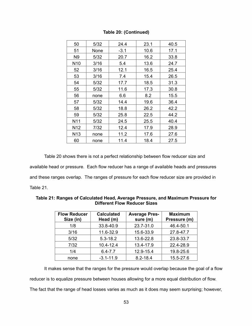
53
Table 20: (Continued)
50 5/32 24.4 23.1 40.5
51 None -3.1 10.6 17.1
N9 5/32 20.7 16.2 33.8
N10 3/16 5.4 13.6 24.7
52 3/16 12.1 16.5 25.4
53 3/16 7.4 15.4 26.5
54 5/32 17.7 18.5 31.3
55 5/32 11.6 17.3 30.8
56 none 6.6 8.2 15.5
57 5/32 14.4 19.6 36.4
58 5/32 18.8 26.2 42.2
59 5/32 25.8 22.5 44.2
N11 5/32 24.5 25.5 40.4
N12 7/32 12.4 17.9 28.9
N13 none 11.2 17.6 27.6
60 none 11.4 18.4 27.5
Table 20 shows there is not a perfect relationship between flow reducer size and
available head or pressure. Each flow reducer has a range of available heads and pressures
and these ranges overlap. The ranges of pressure for each flow reducer size are provided in
Table 21.
Table 21: Ranges of Calculated Head, Average Pressure, and Maximum Pressure for Different Flow Reducer Sizes
Flow Reducer Size (in)
Calculated Head (m)
Average Pres-sure (m)
Maximum Pressure (m)
1/8 33.8-40.9 23.7-31.0 46.4-50.1
3/16 11.6-32.9 15.6-33.9 27.8-47.7
5/32 5.3-18.2 13.6-22.8 23.8-33.7
7/32 10.4-12.4 13.4-17.9 22.4-28.9
1/4 6.4-7.7 12.9-15.4 19.8-25.6
none -3.1-11.9 8.2-18.4 15.5-27.6
It makes sense that the ranges for the pressure would overlap because the goal of a flow
reducer is to equalize pressure between houses allowing for a more equal distribution of flow.
The fact that the range of head losses varies as much as it does may seem surprising; however,
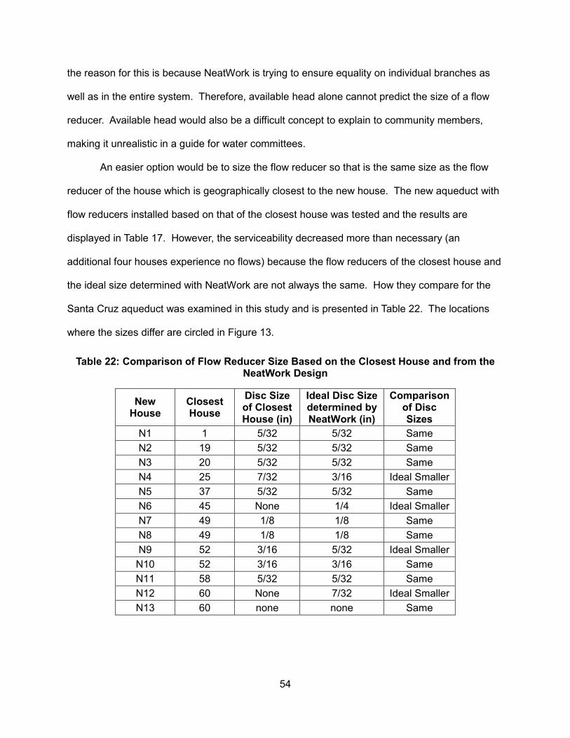
54
the reason for this is because NeatWork is trying to ensure equality on individual branches as
well as in the entire system. Therefore, available head alone cannot predict the size of a flow
reducer. Available head would also be a difficult concept to explain to community members,
making it unrealistic in a guide for water committees.
An easier option would be to size the flow reducer so that is the same size as the flow
reducer of the house which is geographically closest to the new house. The new aqueduct with
flow reducers installed based on that of the closest house was tested and the results are
displayed in Table 17. However, the serviceability decreased more than necessary (an
additional four houses experience no flows) because the flow reducers of the closest house and
the ideal size determined with NeatWork are not always the same. How they compare for the
Santa Cruz aqueduct was examined in this study and is presented in Table 22. The locations
where the sizes differ are circled in Figure 13.
Table 22: Comparison of Flow Reducer Size Based on the Closest House and from the NeatWork Design
New House
Closest House
Disc Size of Closest House (in)
Ideal Disc Size determined by NeatWork (in)
Comparison of Disc Sizes
N1 1 5/32 5/32 Same
N2 19 5/32 5/32 Same
N3 20 5/32 5/32 Same
N4 25 7/32 3/16 Ideal Smaller
N5 37 5/32 5/32 Same
N6 45 None 1/4 Ideal Smaller
N7 49 1/8 1/8 Same
N8 49 1/8 1/8 Same
N9 52 3/16 5/32 Ideal Smaller
N10 52 3/16 3/16 Same
N11 58 5/32 5/32 Same
N12 60 None 7/32 Ideal Smaller
N13 60 none none Same

55
Figure 13: Map of Faucet Locations as Indicated in the Red Circles where Flow Reducer Size Changes from that of Closest House and Ideal Size from NeatWork Design (not to
scale)
With the exception of house N9, the houses where the flow reducer of the closest house
does not match the ideal size are all located towards the end of a branch of the system. These
branches are also sloping upwards, so that the farthest house is higher on the hill as shown in
the slopes leading up to house 29, 45, and 60. This is also reflected in the slopes leading to
house 12 and 16. The house near the end of a branch requires a different flow reducer size
with just a small change in elevation and distance from the closest house. The profiles of these
sections of the aqueduct are displayed in Figures 14-17. While the profiles have different axis,
the slopes are all the same.
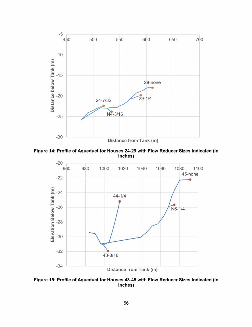
56
Figure 14: Profile of Aqueduct for Houses 24-29 with Flow Reducer Sizes Indicated (in inches)
Figure 15: Profile of Aqueduct for Houses 43-45 with Flow Reducer Sizes Indicated (in inches)
24-7/32
N4-3/16
29-1/4
28-none
-30
-25
-20
-15
-10
-5450 500 550 600 650 700
Dis
tan
ce b
elo
w T
an
k (
m)
Distance from Tank (m)
43-3/16
44-1/4
N6-1/4
45-none
-34
-32
-30
-28
-26
-24
-22
-20960 980 1000 1020 1040 1060 1080 1100
Ele
vati
on
Belo
w T
an
k (
m)
Distance from Tank (m)

57
Figure 16: Profile of Aqueduct for Houses 58-60 with Flow Reducer Sizes Indicated (in inches)
Figure 17: Profile of Aqueduct for Houses 10-16 with Flow Reducer Sizes Indicated (in inches)
58-5/32
59-5/32
N11-5/32
N12-7/32
N13-none
60-none
-50
-45
-40
-35
-30
-251025 1075 1125 1175 1225 1275
Dis
tan
ce f
rom
Tan
k (
m)
Distance from Tank (m)
10-5/32
11-7/32
12-1/4
13-none
14-none
15-3/1616-3/16
-40
-35
-30
-25
-20
-15450 500 550 600 650 700
Dis
tan
ce B
elo
w T
an
k (
m)
Distance from Tank (m)

58
The profiles for houses 10-13 and 14-16 are similar to the other profiles as they all are
end branches that slope upwards. The individual branches also do not have all the flow reducer
sizes represented. However, unlike the other end branches, these branches are geographically
close together and between the two of them include all the flow reducer sizes, which may affect
the new flow reducer sizes. Based on the preceding analysis, the following rules about sizing
flow reducers for future houses were created (and tested later in this research to determine their
validity):
1) Houses in the central area of the distribution system; i.e., a house surrounded by lots of
houses and with multiple houses after it, will have the flow reducer of equivalent size to
that of the closest house. For example, in Figure 13 the new house numbered as N7
has the same size flow reducer as its closest existing house, house 49.
2) Houses added on an end branch, i.e., the last section of a pipe where only a few houses
remain and the topography slopes upward and all flow reducer sizes are not present,
new houses should have the flow reducer size smaller than the house the comes after it.
For example, in Figure 13, the new house numbered N6 has a flow reducer (1/4”) which
is a size smaller than the house that comes after it, house 45 (no flow reducer).
3) Houses added on an end branch where consecutive flow reducer sizes are present in
the region will have the size of the flow reducer based on the size of the house at the
closest elevation. For example, in Figure 13, a house added between houses 14 and
15 at the same elevation as house 11, should have the same flow reducer size as
house 11.
4.2 Analysis of Experiment Houses to Test Rules from Aqueduct Analysis
Rule 1 (that houses placed in the middle of the system will need the same size flow
reducer that is installed in the closest house) did not need to be tested with experiment houses.
New houses N1, N2, N3, and N5 as shown in Figure 12 supported this conclusion in the initial

59
analysis. While house N9 did not support this conclusion, no notable changes in flows
occurred when the ideal flow reducer size was changed for that of the closest house. Since this
had many houses supporting this rule in the initial analysis and it is the easiest to implement, no
tests were performed to test this rule.
To support Rule 2 (that houses added on end branches need a flow reducer sized
smaller than the house that comes after it) experiment houses 1, 2, 3, 5, 6, and 7 identified in
Figure 10 were used. Experiment houses 4, 8, and 9 (Figure 10) tested Rule 3, that new houses
placed in a group of all flow reducer sizes should be sized to match the size of the house
closest in elevation.
To see which flow reducer size worked best and to verify the rules, the author ran
simulations on every design file noting where she had to manually change flow reducer sizes to
match the flow reducer size from the “All” design file. A summary of these results is presented
in Table 23.
Experiment houses 1, 2, 3, 5, 6, and 7 all performed better (Experiments X1, X5, X6, and
X7) or the same (Experiments X2 and X3) with the flow reducer size based on Rule 2 compared
to using the size of the flow reducer installed in the closest house. This supports the validity of
Rule 2.
The experiments performed to test Rule 3, X4, X8, and X9 showed mixed results. For
experiment X4 and X8 the flow reducer size obtained based on the closest house was found to
be better. In experiment X9, the size of the new flow reducer installed in the experiment house
influences the flows of the surrounding houses differently. House P13 was found to experience
flows smaller than 0.1 L/s less frequently with the flow reducer sized based on the closest
house, while P14 experienced flows less than 0.1 L/s more frequently with the same one.
These results show that Rule 3 is not valid in the Santa Cruz aqueduct and that in these areas it
is better to install the flow reducer based on the closest house.
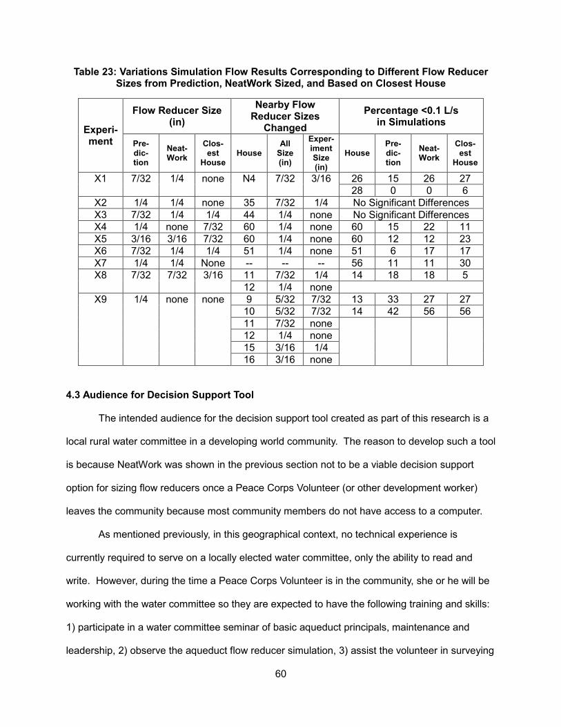
60
Table 23: Variations Simulation Flow Results Corresponding to Different Flow Reducer Sizes from Prediction, NeatWork Sized, and Based on Closest House
Experi-ment
Flow Reducer Size (in)
Nearby Flow Reducer Sizes
Changed
Percentage <0.1 L/s in Simulations
Pre-dic-tion
Neat-Work
Clos-est
House House
All Size (in)
Exper-iment Size (in)
House Pre-dic-tion
Neat-Work
Clos-est
House
X1 7/32 1/4 none N4 7/32 3/16 26 15 26 27 28 0 0 6
X2 1/4 1/4 none 35 7/32 1/4 No Significant Differences X3 7/32 1/4 1/4 44 1/4 none No Significant Differences X4 1/4 none 7/32 60 1/4 none 60 15 22 11 X5 3/16 3/16 7/32 60 1/4 none 60 12 12 23 X6 7/32 1/4 1/4 51 1/4 none 51 6 17 17 X7 1/4 1/4 None -- -- -- 56 11 11 30 X8 7/32 7/32 3/16 11 7/32 1/4 14 18 18 5
12 1/4 none X9 1/4 none none 9 5/32 7/32 13 33 27 27
10 5/32 7/32 14 42 56 56 11 7/32 none
12 1/4 none 15 3/16 1/4 16 3/16 none
4.3 Audience for Decision Support Tool
The intended audience for the decision support tool created as part of this research is a
local rural water committee in a developing world community. The reason to develop such a tool
is because NeatWork was shown in the previous section not to be a viable decision support
option for sizing flow reducers once a Peace Corps Volunteer (or other development worker)
leaves the community because most community members do not have access to a computer.
As mentioned previously, in this geographical context, no technical experience is
currently required to serve on a locally elected water committee, only the ability to read and
write. However, during the time a Peace Corps Volunteer is in the community, she or he will be
working with the water committee so they are expected to have the following training and skills:
1) participate in a water committee seminar of basic aqueduct principals, maintenance and
leadership, 2) observe the aqueduct flow reducer simulation, 3) assist the volunteer in surveying

61
the existing system, 4) know how to cut and mold PVC pipes, and 5) help fabricate and install
flow reducers into the existing system.
Therefore, in order for a decision making tool to be appropriate to be left with the water
committee members it needs to be: 1) relatively simple and easy to understand, 2) not relying
on difficult mathematics, and 3) not relying on understanding of engineering hydraulic concepts
such as available head.
4.4 Assumptions
This tool to size flow reducers was developed to assist the decision making of a local
water committee. In order for it to work effectively, the following assumptions on aqueduct
expansion have to be made:
1) Houses will be placed randomly though the system instead of creating a new branch
with multiple houses
2) Houses will be placed within the existing distribution system (i.e., not farther away from
the tank than any of the existing houses)
3) Houses will be added to the aqueduct based on normal population growth (more
information on how population growth can be used to determine what a reasonable
number of houses that will be added to the aqueduct during its lifespan is in Appendix F).
4.5 Tool to Size Flow Reducers
Based on the proceeding analysis and information, the author created a map tool to size
flow reducers as presented in Figure 18. This map visually depicts the accepted Rule 2 by
marking locations that follow that rule in different colors depending on flow reducer size. The
color coating, makes it possible for those on the water committee to use the map. Using a map
tool in Santa Cruz is culturally appropriate because the water committee is able to use it to size
flow reducers without significant training or relying on skills they do not have. While maps are
not widely used in their culture, the members of the water committee and community

62
demonstrated an ability to use maps when they drew a community map for the author when she
first arrived in Santa Cruz. They also showed understanding of the map tool developed for this
research by properly identifying flow reducer sizes for theoretical future houses during the initial
explanation of the tool. If the as-built aqueduct matched the original designed aqueduct, the
map tool in Figure 18 would have been given to the Santa Cruz water committee.
Figure 18: Final Decision Support Tool Created for the Originally Designed Santa Cruz Aqueduct Presenting Faucet Numbers and Locations where Flow Reducers Cannot Be
Sized Based on the Flow Reducer Size of the Closest House (not to scale)
The following instructions were also translated and provided to the water committee:
Locate where the new house will be on the map and determine the correct size of the flow
reducer using the following rules:
1) If the house was included in the original design and marked by an N#, install flow
reducers as depicted by the symbol.
2) If the new house is not in an oval, install the same size flow reducer of the closest
house.
63
3) If the new house is in a green oval, install a 1/4-inch flow reducer.
4) If the new house is in a yellow oval, install a 7/32-inch flow reducer.
5) If the new house is in a red oval, install a 3/16-inch flow reducer.
4.6 Applying the Tool to the As-Built Aqueduct
Due to a variety of factors, the aqueduct that was actually built does not match the
aqueduct the author initially designed or solicited funds to build. Some of these changes
included moving the storage tank to a higher elevation, changing locations where the pipe was
buried in order to cross a river at a shorter span that reduced costs associated with building a
bridge, changing locations where pipes were placed to follow established footpaths rather than
cutting through people’s land, adding six additional houses to the design from the secondary
aqueduct to help alleviate problems associated with the fact that the source for that system was
drying up, and changing the design because of community input so everyone had individual
connections to the main line rather than connecting to shared branches.
Due to changes in pipe placement during construction, the author used her engineering
judgement based upon the original aqueduct design to install pipes that would allow for a
functioning aqueduct. Midway through the project when the author believed she was aware of
all changes, she created a new NeatWork design file, “Final Design”, based on what was
actually implemented in the field. She then used NeatWork to size the flow reducers on the as-
built system verifying it still would have a high level of service. This design resulted in a
NeatWork simulation with zero houses experiencing no flows or having flows less 0.1 L/s 25%
of the time. The input tables and NeatWork summary report for the final design are in Appendix
D. Small changes were still made during construction in regards to where homeowners wanted
their individual lines to connect to the main line. The author decided these changes would not
affect the level of service associated with the aqueduct or warrant the need to change flow
reducer sizes, so she did not redo the NeatWork design to reflect these minor changes.
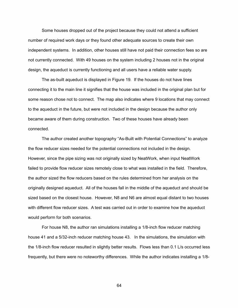
64
Some houses dropped out of the project because they could not attend a sufficient
number of required work days or they found other adequate sources to create their own
independent systems. In addition, other houses still have not paid their connection fees so are
not currently connected. With 49 houses on the system including 2 houses not in the original
design, the aqueduct is currently functioning and all users have a reliable water supply.
The as-built aqueduct is displayed in Figure 19. If the houses do not have lines
connecting it to the main line it signifies that the house was included in the original plan but for
some reason chose not to connect. The map also indicates where 9 locations that may connect
to the aqueduct in the future, but were not included in the design because the author only
became aware of them during construction. Two of these houses have already been
connected.
The author created another topography “As-Built with Potential Connections” to analyze
the flow reducer sizes needed for the potential connections not included in the design.
However, since the pipe sizing was not originally sized by NeatWork, when input NeatWork
failed to provide flow reducer sizes remotely close to what was installed in the field. Therefore,
the author sized the flow reducers based on the rules determined from her analysis on the
originally designed aqueduct. All of the houses fall in the middle of the aqueduct and should be
sized based on the closest house. However, N8 and N6 are almost equal distant to two houses
with different flow reducer sizes. A test was carried out in order to examine how the aqueduct
would perform for both scenarios.
For house N8, the author ran simulations installing a 1/8-inch flow reducer matching
house 41 and a 5/32-inch reducer matching house 43. In the simulations, the simulation with
the 1/8-inch flow reducer resulted in slightly better results. Flows less than 0.1 L/s occurred less
frequently, but there were no noteworthy differences. While the author indicates installing a 1/8-
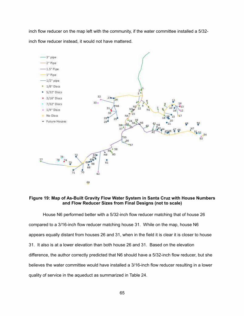
65
inch flow reducer on the map left with the community, if the water committee installed a 5/32-
inch flow reducer instead, it would not have mattered.
Figure 19: Map of As-Built Gravity Flow Water System in Santa Cruz with House Numbers and Flow Reducer Sizes from Final Designs (not to scale)
House N6 performed better with a 5/32-inch flow reducer matching that of house 26
compared to a 3/16-inch flow reducer matching house 31. While on the map, house N6
appears equally distant from houses 26 and 31, when in the field it is clear it is closer to house
31. It also is at a lower elevation than both house 26 and 31. Based on the elevation
difference, the author correctly predicted that N6 should have a 5/32-inch flow reducer, but she
believes the water committee would have installed a 3/16-inch flow reducer resulting in a lower
quality of service in the aqueduct as summarized in Table 24.

66
Table 24: Simulation Differences between Varying Flow Reducer Sizes for House 6 in As-Built Aqueduct
House min flow (L/s) % flows less
than 0.1 L/s (%)
5/32" 3/16" 5/32" 3/16"
10 0.00596 0.74 17 27
11 0 0 51 61
14 0.0639 0.0596 26 50
While an ideally sized flow reducer has better results, this shows that there are some
houses that will not follow the easily recognized guidelines and communities will install flow
reducers that may not be ideal. This may hurt some houses, but it will not destroy the quality of
service of the aqueduct. It can be avoided if the author can determine where the future houses
will be and include them on the map as is what happened in Santa Cruz. The author will reflect
the ideal flow reducer sizes for houses N8 and N6 as well as the other new houses on the map
to be provided to the water committee.
The author analyzed how the new design would affect the circled locations as presented
in Figure 18, the original tool she created. This time, she also took into account the likelihood of
houses being built in these regions based on her personal knowledge of the families. In the
following analysis, the house numbers match those from Figure 19.
Initially there was a circle close to the end branch including houses 51-54. However,
none of these houses are currently connected to the aqueduct and only house 52 expressed
interest in connecting. If a house is built between house 51 and 52, it would most likely require
a 3/16-inch flow reducer assuming all the houses are connected. However, with few houses
connected at the end of the line, the size of the flow reducer installed in that area will have even
less of an impact. A circle may not be necessary.
Looking at end branch with houses 73-77, one notices that an additional house was
added even though the residents originally wanted to stay on their independent system. House

67
77 is actually significantly lower in elevation than house 75 and 76, hence the smaller flow
reducer size. If a house were to be built between house 75 and 76, it would most likely be a
flow reducer sized at either 5/32-inch or 3/16-inch depending on elevation. Marking two
different sizes in an area so close together becomes more complicated for the local water
committee, especially when passed down to future committees who were not trained by the
author. The author does not believe it is very likely a house will be built there because it is the
land of the family that lives in house 77 and they have no children making the circles potentially
more confusing than necessary.
In the new design, no flow reducer sizes are skipped between house 73 and 76.
Therefore, unlike in the original tool, it is appropriate to size any new houses built in this area
based on the size of the flow reducer of the closest house.
The circle that was on the map between the existing house 26 and N6 is no longer
relevant because it no longer is at an end branch. Also, the circle that was before house 32
seems irrelevant because this land is being used as a cooperative farm. It is unlikely that
anyone will build a house there and it has its own system from an open stream to water its crops
and give to the animals. Therefore, it will not require its own connection either.
This leaves the circles leading to houses 62 and 69. While these circles would be
relevant, adding them increases the complexity of the tool, but would only minimally affect the
aqueducts serviceability especially since house 69 is not currently connected. After working
with the water committee on installing the flow reducers and seeing how the current aqueduct is
working, the author believes that having a few flow reducers installed of non-ideal size will be
okay. Therefore, she opted for the simplest map option and removed the circles leading to
houses 62 and 69 as well. She renumbered the map as shown in Figure 20 and left copies with
different individuals of the water committee with the following translated instructions and list of

68
the owners’ names as they correspond to each number. She also gave them a letter explaining
the importance of continually installing flow reducers.
Figure 20: Map with House Numbers and Flow Reducer Sizes Provided to the Santa Cruz Water Committee (not to scale)
The instructions to use with the map in Figure 20 are:
1) If a new house is shown on the map, install the flow reducer as indicated.
2) If a new house is not shown on the map install the same size flow reducer that the house
closest to it has.
Along with the map, the author also left many prefabricated flow reducers of all sizes in
Ziplock™ bags labeled with the flow reducer size. Inside, was also a piece of paper colored to
match the symbol on the map as seen in Figure 21.

69
Figure 21: Picture of Extra Flow Reducers Provided to the Santa Cruz's Water Committee

70
Chapter 5: Conclusions and Recommendations
Many Peace Corps Volunteers in Panama use flow reducers in gravity flow water
distribution systems they improve and build. While flow reducers help equalize the flows
between houses, they need to be installed in any future connections to ensure systems remain
reliable. The objectives of this thesis were: 1) Use the NeatWork model to determine how the
addition of houses to an existing gravity flow water system will affect its serviceability, 2)
Develop an easy to understand method to teach community members from Santa Cruz
(Panama) in order to enable community members to correctly size flow reducers for houses
added to the water system in the future, and 3) Provide guidance to future Peace Corps
Volunteers and development workers to ensure they are able to design and implement
sustainable flow reducer projects in their respective communities. These objectives were
designed to disseminate the knowledge generated in this research to two distinct stakeholders:
a water committee comprised of community members whose job is to maintain the aqueduct
with Objective 2 and development workers who will plan and lead the implementation of the
projects as well as train local water committees through Objective 3.
5.1 Conclusions from Objective 1
As expected, as more houses are added to an existing aqueduct, the service quality
declines. However, the declines in serviceability can be reduced if community members
continually install flow reducers during the expansion. The closer the installed flow reducers are
to their ideal size, the smaller the effect on serviceability will be. Objective 2 explores how to
ensure the right size flow reducers will be installed.
71
As houses are added, the ideal pipe sizes will also increase in certain parts of the
system. While it is impractical, to design a system that would require pipes to be changed after
installation, the designer can include future installations in the initial design to create a more
robust system from the beginning. Before surveying, the system designer should talk to their
community about where houses may be built in the future and include these and all houses in
construction in the original design. This will create an aqueduct design with some pipes larger
than those required at the moment, but it will allow for expansion without hurting serviceability,
helping long term sustainability.
Some future connections will be missed as it will not be possible to correctly identify
where and when houses will be built. Although the ideal design will change, the author
concludes that this is acceptable as desired changes within the pipe network are minimal and
serviceability remains good as long as flow reducers are continually installed.
5.2 Conclusions from Objective 2
Due to the complexity of water distribution systems and the limited technical knowledge
of water committee members, it was not possible to create a uniform decision support tool to
use with all distribution systems. However, based on the analysis, a map can be created for
individual aqueducts and left with the community’s water committee as presented in Section 4.4.
The map presents the correct flow reducer size determined by NeatWork for any known
potential connection as well as well as providing instructions on how to size houses that were
not included in the original design.
In the Santa Cruz aqueduct, the author observed that end branches that slope upwards
and areas without all the flow reducer sizes are more sensitive to flow reducer sizes being
different than that of the closest house. She also noted that some end branches were similar in
topography, but differed because while on different branches the region had all the flow reducer
72
sizes which might lead to sizing houses based on the flow reducer size of the house at the
closest elevation.
Based on her observations, the author developed three rules to size flow reducers which
were then tested with experimental houses. In the majority of the aqueduct system studied
here, any new house can have the same size flow reducer of the closest house. This was seen
in the original analysis when eight of the thirteen new houses had the same flow reducer size
when sized with NeatWork and by sizing based on the flow reducer size of the closet house.
Installing flow reducers based on the closest house became the basis for Rule 1. With the
results from this analysis on the experiment houses, it can be concluded that Rule 2 is valid; in
the sloping upwards end branches, flow reducer sizes closer to the tank should be smaller in
size than the house after it. Rule 3, that in some areas flow reducers should be sized based on
the flow reducer size installed in the house that is closest in terms of elevation, was rejected
based on the experiments.
In order to turn the rules into a tool that can be used by the local water committee a
map tool was created that visually depicts them. It allows water committee members to size
flow reducers themselves making it culturally appropriate.
5.3 Conclusions from Objective 3
A guide was developed for sustainable flow reducer projects that was disseminated for
future volunteers based on the research for this thesis and the author’s experience from
manufacturing and installing flow reducers in the Santa Cruz community. The guide is
reproduced as Appendix A and the main points are summarized below:
1) Include all potential future connections considering houses with independent sources,
houses under construction, and spots where houses may be built in the future.
2) Teach the entire community, not just the water committee about the importance of flow
reducers and include all community members in the fabrication of the flow reducers.
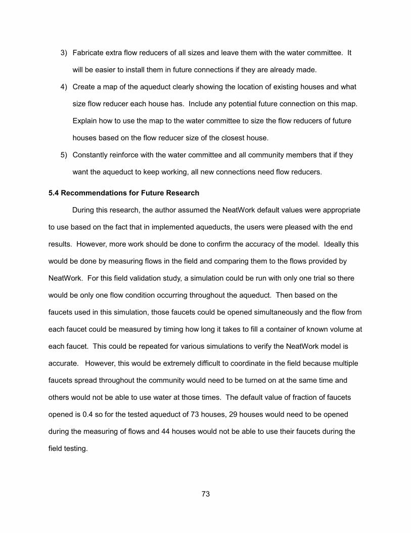
73
3) Fabricate extra flow reducers of all sizes and leave them with the water committee. It
will be easier to install them in future connections if they are already made.
4) Create a map of the aqueduct clearly showing the location of existing houses and what
size flow reducer each house has. Include any potential future connection on this map.
Explain how to use the map to the water committee to size the flow reducers of future
houses based on the flow reducer size of the closest house.
5) Constantly reinforce with the water committee and all community members that if they
want the aqueduct to keep working, all new connections need flow reducers.
5.4 Recommendations for Future Research
During this research, the author assumed the NeatWork default values were appropriate
to use based on the fact that in implemented aqueducts, the users were pleased with the end
results. However, more work should be done to confirm the accuracy of the model. Ideally this
would be done by measuring flows in the field and comparing them to the flows provided by
NeatWork. For this field validation study, a simulation could be run with only one trial so there
would be only one flow condition occurring throughout the aqueduct. Then based on the
faucets used in this simulation, those faucets could be opened simultaneously and the flow from
each faucet could be measured by timing how long it takes to fill a container of known volume at
each faucet. This could be repeated for various simulations to verify the NeatWork model is
accurate. However, this would be extremely difficult to coordinate in the field because multiple
faucets spread throughout the community would need to be turned on at the same time and
others would not be able to use water at those times. The default value of fraction of faucets
opened is 0.4 so for the tested aqueduct of 73 houses, 29 houses would need to be opened
during the measuring of flows and 44 houses would not be able to use their faucets during the
field testing.

74
Another option would be to compare the flows if only one faucet was opened. In
NeatWork an individual faucet simulation could be run and in the field flow could be measured
for individual faucets. To guarantee only one faucet would be in use during the field test without
disrupting the daily lives of the community members it is recommended that flow from the
designated faucet be measured at night when most of the community is sleeping.
Another consideration when collecting flow data in the field would be the height of the
water in the tank. The NeatWork model assumes that the level of water is at the elevation of the
tank outlet where it provides the minimal head. The outlet is typically located close to the bottom
of the storage tank. Most likely the storage tank will have more water in it providing additional
head and potentially greater flow in the distribution system. Two simulations could be run in
NeatWork changing the elevation of the tank to match the elevation of the outlet and the
overflow to calculate the minimum and maximum flow at each faucet. The measured flow
should fall in this range of values. If this range is too large to verify the accuracy of the results, it
could also be coordinated for the water levels in the tank to be monitored while flow
measurements are being collected and changing the height of the tank to match this height
before running the NeatWork simulation. Collecting flow measurements in the field would help
to validate NeatWork’s ability to provide accurate flows.
To further validate this research, a sensitivity analysis should be run to test the two most
important input values which are expected to be the service factor, which is used during the
design phase and the fraction of faucets opened, which is used during the simulation phase.
These two variables are related to the serviceability of the aqueduct.
A larger service quality factor corresponds to a more reliable aqueduct, but it will also be
more expensive. The design engineer typically wants to use a value that provides sufficient
water without wasting money. Also, as more faucets are opened, the serviceability of the
system will decrease. While it is more economical to design an aqueduct assuming all of the

75
faucets are not open at the same time, it is important that the fraction of faucets open is an
accurate representation of community behavior. If it is too low, the model will show the
aqueduct providing everyone in the community with water when in reality users may face low or
no flow situations. Along with a sensitivity analysis, surveys of users could be conducted
collecting information regarding when people use water and times when the flow is too low.
This thesis works under the assumption that houses will be added to the aqueduct, and if
they are properly sized with flow reducers, the aqueduct will continue functioning at a
reasonable level of service. However, at some point too many additional houses will cause the
aqueduct to be undersized and houses will cease to have a reliable flow. More research should
be conducted to determine what this limit is and potentially determine how Peace Corps
Volunteers can alter initial designs to compensate for the additional houses that may be added
in the future after Peace Corps has left the community. Also, work could be done to determine
how to add branches to an aqueduct rather than having new houses randomly placed
throughout the distribution network.
While the author was able to create a map tool for the Santa Cruz community, more work
needs to be done to determine if there is a generic way to create map tools for other
communities regardless of aqueduct size and layout. Depending on results and if it is deemed
necessary to use the map tool instead of sizing based on the closest house, guides should be
developed for future Peace Corps Volunteers to help them recreate the map tool as presented
for their respective communities.
Monitoring and evaluation needs to be continued to see how communities respond to the
flow reducer projects years in the future. Are they installing flow reducers as houses are
added? Are they sizing them correctly? Have flow reducers been removed from the system?
Environmental Health Volunteers have been working in Panama since 2002. While it is
unknown exactly when Peace Corps Volunteers started installing flow reducer projects, the

76
author knows they have been utilized since 2011 making some systems at least 5 years old.
For these systems, data can be collected about how the aqueduct has expanded since initial
implementation, if the aqueduct is still operating at a reliable level of service, if flow reducers
have been removed for any reason, if flow reducers have been installed in any new
connections, what sort of trainings were done relating to flow reducers, etc. In a few years
monitoring and evaluation should be performed in Santa Cruz and other communities that have
implemented flow reducer projects under the guidance of this research. It should be
investigated what the volunteer did to assist the water committee with flow reducer maintenance
and see how the water committee is doing. Do they still use the map tool when houses are
added? Was the information successfully passed down to future water committee members?
Monitoring and evaluation will be required to determine how sustainable the projects actually
are and will allow for improvements to be made to the volunteer guide and community map tool
to make future projects more successful.
A challenging aspect of this research was dealing with NeatWork. While it is a great tool
for the design of distribution systems in this setting, the software is outdated and can be
frustrating to use. The latest version of NeatWork was released in 2010 and has not been
updated while computer processors have. Therefore, there are some compatibility issues
causing NeatWork to freeze frequently. Inputting pipe constraints is also a tedious process as
the sizes need to be manually imput for each segment length. While it is still a viable option
with many advantages, it may be worthwhile to think about contacting Agua Para La Vida to
help update NeatWork to make it more user-friendly.
It might be beneficial for other researchers to look into adapting other software such as
EPANET or GOODwater for situations like explored in this research. EPANET is another
publicly available computer software created for use in the developed world on larger systems.
The author knows some Peace Corps Volunteers have used EPANET to aide in their aqueduct

77
design, but is not sure exactly what capabilities it has in regards to sizing flow reducers and
running simulations.
GOODwater was developed by a Master’s International Peace Corps Volunteer to
optimize pipe sizing utilizing the solver function in Excel. It currently does not allow for valves or
flow reducers to be utilized in the design. A future researcher would need to modify the
GOODwater software in order to apply it to similar research. If either EPANET of GOODwater
can be applied to flow reducer research, it might make further analysis faster.

78
List of References
Agua Para La Vida. “Home”. Agua Para La Vida, 2014. Web. 19. Oct. 2016. <aplv.org> Agua Para La Vida. “NeatWork: A User Guide”. Agua Para La Vida, 2010. Web. 3 Nov. 2014. <http://neatwork.ordecsys.com/dl/neatworkuserguide.pdf?q=neatwork/dl/neatworkuserguide.pdf> Agua Para La Vida and ORDECSYS. “Neatwork Water Distribution Network”. Agua Para La Vida, 2010. Web. 27. Sept. 2016. <http://neatwork.ordecsys.com/download.html> Annis, J.E. Assessing Progress of Community Managed Gravity Flow Water Supply Systems using Rapid Rural Appraisal in the Ikongo District. Thesis. Michigan Technological University, 2006. Web. 30 Nov. 2014. <http://cee.eng.usf.edu/peacecorps/5%20-%20Resources/Theses/Water/2006Annis.pdf> Atkinson, S. A Futures Approach to Water Distribution and Sewer Network (Re)Design. Thesis. University of Exeter, 2013. Web. 3 Nov. 2014. <https://ore.exeter.ac.uk/repository/handle/10871/10730> Breslin, E.D. “The Demand-Responsive approach in Mozambique: Why choice of technology matters”. UNICEF WATERfront, 2003 16: 9-12. Web. 3 Nov. 2014. <http://www.unicef.org/wash/files/wf16e.pdf> Bentley. “WaterCad V8i”. Bentley, 2014. Web. 27 Oct. 2014. <http://www.bentley.com/en-US/Products/WaterCAD/> CIA World Factbook. "Central America and Caribbean: Panama". The World Factbook. Central Intelligence Agency, 2014. Web. 1 Oct. 2014. <https://www.cia.gov/library/publications/the-world-factbook/geos/pm.html> Crowe, T.T., Elger, D.F., Williams, B.C., and Roberson, J.A. “Flowing Fluids and Pressure Variations”, “Flow in Conduits”, and “Flow Measurements”. Engineering Fluid Mechanics, 9th ed. Wiley, New York, 2010. pp. 77-114, 315-351, 435-464. DNV GL. “SynerGEE Water”. DNV GL, 2010. Web. 27 Oct. 2014. <http://www.gl-group.com/en/water/SynerGEEWater.php> Environmental Protection Agency (EPA). “Drinking Water Distribution Systems”. EPA, 2014a. Web. 13 Oct 2014. <http://water.epa.gov/lawsregs/rulesregs/sdwa/tcr/distributionsystems.cfm>

79
Environmental Protection Agency (EPA). “EPANET”. EPA, 2014b. Web. 27 Oct. 2014. <http://www.epa.gov/nrmrl/wswrd/dw/epanet.html> Faiia, S. “Practical Design Notes for Simple Rural Water Systems. Attachment 34-A”. CARE: Indonesia, 1982. Fry, L.M., Cowden, J.R., Watkins, D.W., Clasen, T. and Mihelcic, J.R. "Quantifying Health Improvements from Water Quantity Enhancement: An Engineering Perspective Applied to Rainwater Harvesting in West Africa”. Environmental Science and Technology, 2010 44(24): 9535-541. Good, S.P. Development of a Decision Support System for Sustainable Implementation of Rural Gravity Flow Water Systems. Thesis. Michigan Technological University, 2008. Web. 30 Nov. 2014. <http://cee.eng.usf.edu/peacecorps/5%20-%20Resources/Theses/Water/2008Good.pdf> Google Maps. “8°39'13.2"N, 80°22'01.4"W”. Google, INEGI, 2016. Web. 27. Sept. 2016. <https://www.google.com/maps/place/8%C2%B039'13.2%22N+80%C2%B022'01.4%22W/@9.9943245,-84.0388517,5z/data=!4m6!3m5!1s0x0:0x0!7e2!8m2!3d8.6536629!4d-80.3670502> Green, K. Embodied Energy Assessment of Rainwater Harvesting Systems in Primary School Settings on La Peninsula, Valiente, Comarca Ngöbe Bugle, Republic of Panama. Thesis. University of South Florida, 2011. Web. 30 Nov. 2014. <http://scholarcommons.usf.edu/etd/3127/> Guillén, L. “Análisis Ambiental y Social Programa de Agua Potable y Saneamiento Rural E Indígena En Panamá”. Ministerio de Salud (MINSA), 2012. Web. 1 Oct 2014. <http://www.minsa.gob.pa/sites/default/ files/ proyectos/aas_pn-g1003.pdf>. Hayman, S. Evaluation of Hand Augered Well Technologies’ Capacity to Improve Access to Water in Coastal Ngöbe Communities in Panama. Thesis. University of South Florida, 2014. Web. 30 Nov. 2014. <http://scholarcommons.usf.edu/etd/3127/> Hokanson, D.R., Mihelcic J.R, and Phillips L.D. “Educating Engineers in the Sustainable Futures Model with a Global Perpective: Education, Research & Diversity Initiatives,” International Journal of Engineering Education, 2007 23(2): 254-265. Innovyze. “Infowater: Modeling made Easy”. Innovyze, 2014. Web. 30 Oct. 2014. <http://www.innovyze.com/products/infowater/> Jordan, T. Handbook of Gravity-Flow Water Systems. Practical Action Publishing, Warwickshire, UK, 1984 Lee, E. and Schwab K. “Deficiencies in drinking water distribution systems in developing countries”. Journal of Water and Health, 2005 3(2): 109-127.

80
Manser, N., Naughton, C., Prouty, C., Orner, K., Verbyla, M., and Mihelcic, J.R. “Improving the Global Competency of Graduate Engineers Through Peace Corps Partnership and Long-Term International Service. Making Value for Society”. Proceedings of the American Society for Engineering Education (ASEE) National Conference, Washington Convention Center, Seattle, WA, June, 2015. McConville, J.R, and Mihelcic, J.R. “Adapting Life-Cycle Thinking Tools to Evaluate Project Sustainability in International Water and Sanitation Development Work”. Environmental Engineering Science, 2007 24(7): 937-948. Mihelcic, J.R. and Zimmerman, J.B. Environmental Engineering: Fundamentals, Sustainability, Design, 2nd Edition, John Wiley & Sons, 2014. Mihelcic, J.R., Myre E.A., Fry L.M., Phillips L.D., Barkdoll, B.D. Field Guide in Environmental Engineering for Development Workers: Water, Sanitation, Indoor Air. American Society of Civil Engineers. (ASCE) Press, Reston, VA, 2009 Mihelcic, J.R., Phillips L.D., Watkins, D.W. “Integrating a Global Perspective into Engineering Education & Research: Engineering International Sustainable Development”. Environmental Engineering Science, 2006 23(3): 426-438. Mihelcic, J.R. “The Right Thing to Do: Graduate Education and Research in a Global and Human Context”. What Is Global Engineering Education For? The Making of International and Global Engineering Educators (Eds: G.L. Downey and K. Beddoes), Morgan & Claypool Publishers, San Francisco, 2010, pp. 235-250. Ministerio de Salud (MINSA). “Decreto Ejecutivo Numero 40”. MINSA, 1994. Niskanen, M.A. “The Design, Construction, and Maintenance of a Gravity-Fed Water System in the Dominican Republic”. Report. Michigan Technological University, 2003. Web. 25 Nov. 2014. <http://usfmi.weebly.com/thesesreports.html> Orner, K. Effectiveness of In-Line Chlorination of Gravity Flow Water Supply in Two Rural Communities in Panama. Thesis. University of South Florida, 2011. Web. 30 Nov. 2014. <http://scholarcommons.usf.edu/etd/3271/> Ostfeld, A., Kogan, U., and Shamir, U. “Reliability Simulation of Water Distribution Systems-Single and Multiquality”. Urban Water, 2002 4(1): 53–61. Reca, J., Martínez, J., Baños R., and Gil, C. “Optimal Design of Gravity-Fed Looped Water Distribution Networks Considering the Resilience Index”. Journal of Water Resources Planning and Management, 2008 134(3): 234-238. Redmond, L. “Your Assignment: Panama, Environmental Health”. Peace Corps, 2012. Reents, N.W. “Design of Potable Water Systems in Honduras”. Report. Michigan Technological University, 2003. Web. 25 Nov. 2014. <http://cee.eng.usf.edu/peacecorps/5%20-%20Resources/Theses/Water/2003Reents.pdf>

81
Santana, M.V.E. The Effect of Urbanization on the Embodied Energy of Drinking Water in Tampa, Florida. Thesis. University of South Florida, 2015. Web. 17 Aug. 2015. <http://scholarcommons.usf.edu/etd/5772/> Santana, M.V.E., Zhang, Q., and Mihelcic, J.R. “Influence of Water Quality on the Embodied Energy of Drinking Water Treatment”. Environmental Science & Technology, 2014(48): 3084-3091. Schweitzer, R.W. Community Managed Rural Water Supply Systems in the Dominican Repub-lic: Assessment of Sustainability of Systems Built by the National Institute of Potable Water and Peace Corps, Dominican Republic. Thesis. University of South Florida, 2009. Web. 25 Nov. 2014. <http://scholarcommons.usf.edu/etd/4765/> Schweitzer, R.W. and Mihelcic J.R. “Sustainability Analysis of Community Managed Water Systems in the Developing World”. Journal of Water, Sanitation and Hygiene for Development, 2012 2(1): 20-30. Simpson, J.D. “Technical Capacity Building of Existing Gravity-Fed Rural Drinking Water Systems in Honduras”. Report. Michigan Technological University, 2003. Web. 25 Nov. 2014. <http://cee.eng.usf.edu/peacecorps/5%20-%20Resources/Theses/Water/2003Simpson.pdf> Suzuki, R. Post-Project Assessment and Follow-Up Support for Community Managed Rural Water Systems in Panama. Thesis. Michigan Technological University, 2010. Web. 30 Nov. 2014. <http://cee.eng.usf.edu/peacecorps/5%20%20Resources/Theses/Assessment/2009Suzuki.pdf> The Engineering ToolBox. “PVC Pipes – Friction Loss and Flow Velocities Schedule 40”. The Engineering ToolBox, 2016. Web. 7 Jul. 2016. <http://www.engineeringtoolbox.com/pvc-pipes-friction-loss-d_802.html> UNICEF and WHO. “25 Years Progress on Drinking Water and Sanitation 2015 Update and MDG Assessment”. UNICEF, 2015. Web. 29 Jun. 2016. <http://files.unicef.org/publications/files/Progress_on_Sanitation_and_Drinking_Water_2015_Update_.pdf> United Nations. “64/292 The human right to water and sanitation”. United Nations General As-sembly, 108th plenary meeting, July 2010. United Nations Development Program. “Sustainable Development Goals 17 Goals to Transform our World”. United Nations, 2015. Web. 27. Sept. 2016. < http://www.un.org/sustainabledevel-opment/water-and-sanitation/> United Nations. “We Can End Poverty Millennium Development Goals and Beyond 2015”. United Nations, 2015. Web. 27 Sept. 2016. < http://www.un.org/millenniumgoals/environ.shtml> University of South Florida. “University of South Florida – Master’s International Program in Civil & Environmental Engineering”. Resources: Thesis/Reports. University of South Florida, 2014. Web. 27 Sept. 2016. <http://usfmi.weebly.com/thesesreports.html>

82
Water for the World. “Designing Community Distribution Systems Technical Note No. RWS 4.D.4”. Water for the World, 2005. Web. 3 Nov. 2014. <https://www.lifewater.org/resources/rws4/rws4d4.pdf> World Bank. “Efficient, Sustainable Service for All? An OED Review of the World Bank’s Assistance to Water Supply and Sanitation. Operations Evaluation Department”. The World Bank, Report No. 26443, 2003. World Bank. “GINI Index”. World Bank, 2014. Web. 25 Oct. 2014. <http://data.worldbank.org/in-dicator/SI.POV.GINI> Yoakum, B.A. Improving Implementation of a Regional In-Line Chlorinator in Rural Panama Through Development of a Regionally Appropriate Field Guide. Thesis. University of South Florida, 2013. Web. 25 Nov. 2014. <http://scholarcommons.usf.edu/etd/4969/>

83
Appendix A: Peace Corps Volunteer Guide to Sustainable Flow Reducer Projects

84

85

86

87

88

89

90
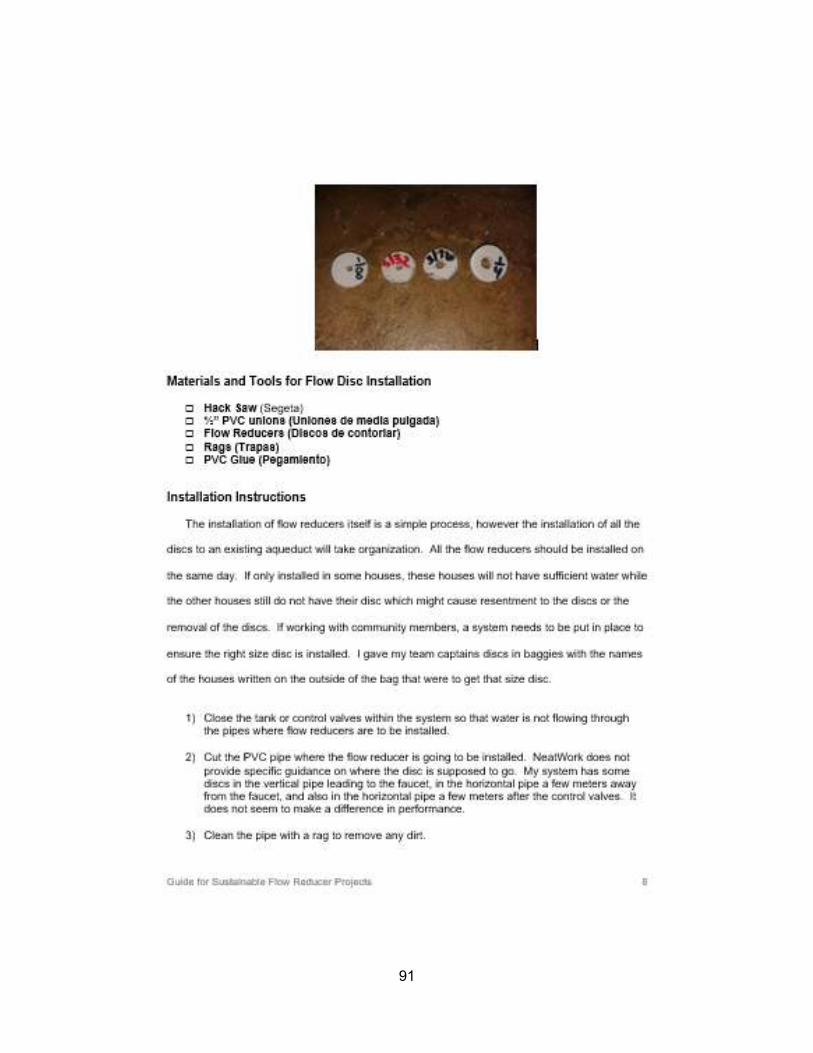
91

92

93

94

95

96
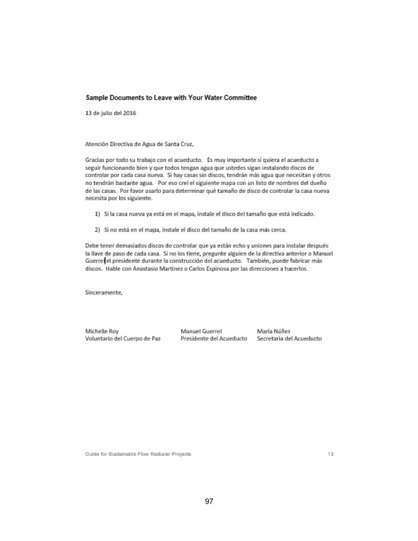
97

98

99

100

101
Appendix B: NeatWork Topography Input Tables for “As Is” and “All” Files
Table B1: Node Input Table to Create NeatWork “As Is” Topography File
T 0.00 0 0 0 0
N1 -4.01 0 0 0 1
N2 -2.62 0 0 0 1
N3 -24.59 0 0 0 1
N4 -26.14 0 0 0 1
N5 -27.71 0 0 0 1
N6 -27.53 0 0 0 1
N7 -27.38 0 0 0 1
N8 -28.35 0 0 0 1
N9 -32.49 0 0 0 1
N10 -36.12 0 0 0 1
N11 -47.12 0 0 0 1
N12 -46.23 0 0 0 1
N13 -46.13 0 0 0 1
N14 -45.67 0 0 0 1
N15 -45.34 0 0 0 1
N16 -37.11 0 0 0 1
N17 -33.78 0 0 0 1
N18 -27.25 0 0 0 1
N19 -26.09 0 0 0 1
N20 -45.72 0 0 0 1
N21 -36.68 0 0 0 1
N22 -31.90 0 0 0 1
N23 -46.15 0 0 0 1
N24 -46.71 0 0 0 1
N25 -27.89 0 0 0 1
N26 -27.89 0 0 0 1
N27 -33.58 0 0 0 1
N28 -36.88 0 0 0 1
N29 -38.35 0 0 0 1
N30 -38.86 0 0 0 1
N31 -37.13 0 0 0 1
N32 -49.48 0 0 0 1
N33 -29.26 0 0 0 1
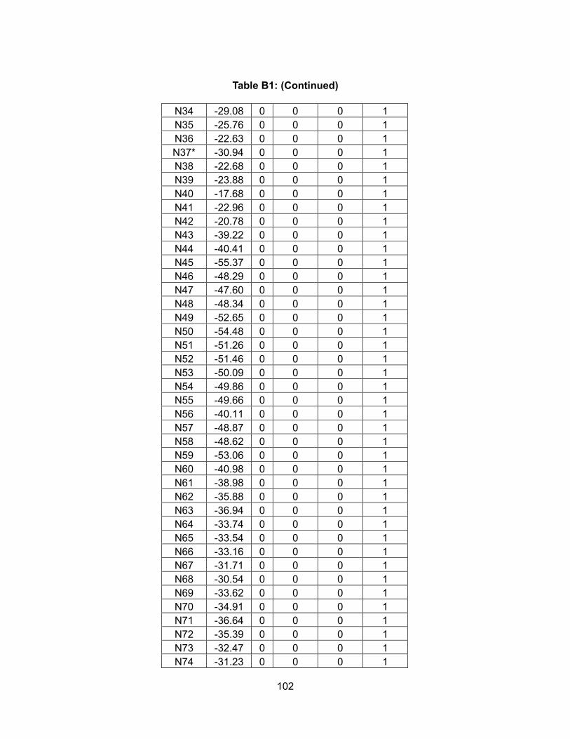
102
Table B1: (Continued)
N34 -29.08 0 0 0 1
N35 -25.76 0 0 0 1
N36 -22.63 0 0 0 1
N37* -30.94 0 0 0 1
N38 -22.68 0 0 0 1
N39 -23.88 0 0 0 1
N40 -17.68 0 0 0 1
N41 -22.96 0 0 0 1
N42 -20.78 0 0 0 1
N43 -39.22 0 0 0 1
N44 -40.41 0 0 0 1
N45 -55.37 0 0 0 1
N46 -48.29 0 0 0 1
N47 -47.60 0 0 0 1
N48 -48.34 0 0 0 1
N49 -52.65 0 0 0 1
N50 -54.48 0 0 0 1
N51 -51.26 0 0 0 1
N52 -51.46 0 0 0 1
N53 -50.09 0 0 0 1
N54 -49.86 0 0 0 1
N55 -49.66 0 0 0 1
N56 -40.11 0 0 0 1
N57 -48.87 0 0 0 1
N58 -48.62 0 0 0 1
N59 -53.06 0 0 0 1
N60 -40.98 0 0 0 1
N61 -38.98 0 0 0 1
N62 -35.88 0 0 0 1
N63 -36.94 0 0 0 1
N64 -33.74 0 0 0 1
N65 -33.54 0 0 0 1
N66 -33.16 0 0 0 1
N67 -31.71 0 0 0 1
N68 -30.54 0 0 0 1
N69 -33.62 0 0 0 1
N70 -34.91 0 0 0 1
N71 -36.64 0 0 0 1
N72 -35.39 0 0 0 1
N73 -32.47 0 0 0 1
N74 -31.23 0 0 0 1
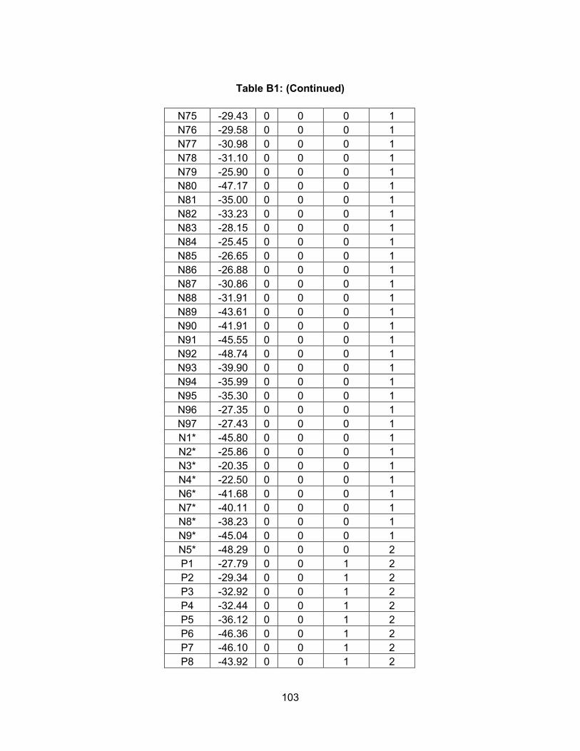
103
Table B1: (Continued)
N75 -29.43 0 0 0 1
N76 -29.58 0 0 0 1
N77 -30.98 0 0 0 1
N78 -31.10 0 0 0 1
N79 -25.90 0 0 0 1
N80 -47.17 0 0 0 1
N81 -35.00 0 0 0 1
N82 -33.23 0 0 0 1
N83 -28.15 0 0 0 1
N84 -25.45 0 0 0 1
N85 -26.65 0 0 0 1
N86 -26.88 0 0 0 1
N87 -30.86 0 0 0 1
N88 -31.91 0 0 0 1
N89 -43.61 0 0 0 1
N90 -41.91 0 0 0 1
N91 -45.55 0 0 0 1
N92 -48.74 0 0 0 1
N93 -39.90 0 0 0 1
N94 -35.99 0 0 0 1
N95 -35.30 0 0 0 1
N96 -27.35 0 0 0 1
N97 -27.43 0 0 0 1
N1* -45.80 0 0 0 1
N2* -25.86 0 0 0 1
N3* -20.35 0 0 0 1
N4* -22.50 0 0 0 1
N6* -41.68 0 0 0 1
N7* -40.11 0 0 0 1
N8* -38.23 0 0 0 1
N9* -45.04 0 0 0 1
N5* -48.29 0 0 0 2
P1 -27.79 0 0 1 2
P2 -29.34 0 0 1 2
P3 -32.92 0 0 1 2
P4 -32.44 0 0 1 2
P5 -36.12 0 0 1 2
P6 -46.36 0 0 1 2
P7 -46.10 0 0 1 2
P8 -43.92 0 0 1 2

104
Table B1: (Continued)
P9 -34.57 0 0 1 2
P10 -35.48 0 0 1 2
P11 -26.04 0 0 1 2
P12 -23.19 0 0 1 2
P13 -20.85 0 0 1 2
P14 -20.09 0 0 1 2
P15 -31.09 0 0 1 2
P16 -29.49 0 0 1 2
P17 -44.78 0 0 1 2
P18 -45.92 0 0 1 2
P19 -46.02 0 0 1 2
P20 -27.89 0 0 1 2
P21 -31.37 0 0 1 2
P22 -35.53 0 0 1 2
P23 -29.87 0 0 1 2
P24 -22.38 0 0 1 2
P25 -23.06 0 0 1 2
P26 -17.32 0 0 1 2
P27 -19.05 0 0 1 2
P28 -18.01 0 0 1 2
P29 -19.81 0 0 1 2
P30 -48.31 0 0 1 2
P31 -48.62 0 0 1 2
P32 -40.98 0 0 1 2
P33 -38.57 0 0 1 2
P34 -36.74 0 0 1 2
P35 -34.58 0 0 1 2
P36 -34.23 0 0 1 2
P37 -30.24 0 0 1 2
P38 -35.70 0 0 1 2
P39 -35.29 0 0 1 2
P40 -36.79 0 0 1 2
P41 -33.69 0 0 1 2
P42 -39.03 0 0 1 2
P43 -31.92 0 0 1 2
P44 -25.18 0 0 1 2
P45 -22.21 0 0 1 2
P46 -47.45 0 0 1 2
P47 -48.34 0 0 1 2
P48 -48.36 0 0 1 2

105
Table B1: (Continued)
P49 -49.25 0 0 1 2
P50 -40.49 0 0 1 2
P51 -17.07 0 0 1 2
P52 -25.40 0 0 1 2
P53 -26.52 0 0 1 2
P54 -31.30 0 0 1 2
P55 -30.81 0 0 1 2
P56 -15.47 0 0 1 2
P57 -36.38 0 0 1 2
P58 -42.23 0 0 1 2
P59 -44.15 0 0 1 2
P60 -27.48 0 0 1 2
Table B2: Arc Length Input Table to Create Neatwork “As Is” Topography File
T N1 14.85
N1 N2 17.20
N2 N3 93.54
N3 N4 12.20
N4 N5 24.40
N5 N6 11.60
N6 N7 6.70
N7 N8 22.10
N8 N9 42.70
N9 N10 25.77
N10 N11 100.76
N11 N12 48.80
N12 N13 12.20
N13 N14 15.00
N14 N15 6.10
N15 N16 38.92
N16 N17 21.49
N17 N18 30.50
N18 N19 18.30
N12 N20 37.48
N20 N21 30.01
N21 N22 23.38
N12 N23 32.61
N23 N24 33.85
N8 N25 12.20

106
Table B2: (Continued)
N25 N26 33.43
N26 N27 48.80
N27 N28 5.00
N28 N29 42.85
N29 N30 4.50
N30 N31 7.80
N31 N32 34.08
N32 N33 59.35
N33 N34 6.10
N34 N35 20.70
N35 N36 35.90
N36 N37* 36.25
N36 N38 1.55
N38 N39 10.07
N39 N40 103.24
N35 N41 48.80
N41 N42 42.70
N30 N43 2.30
N43 N44 18.30
N44 N45 16.08
N45 N46 37.20
N46 N47 30.50
N47 N48 40.00
N48 N49 50.00
N49 N50 4.20
N50 N51 139.00
N51 N52 21.35
N52 N53 18.30
N53 N54 18.30
N54 N55 6.10
N55 N56 79.85
N46 N57 12.20
N57 N58 18.70
N58 N59 49.10
N59 N60 52.55
N60 N61 21.35
N61 N62 29.95
N62 N63 8.53
N62 N64 35.75
N64 N65 7.10

107
Table B2: (Continued)
N65 N66 47.80
N66 N67 24.40
N67 N68 42.70
N68 N69 46.79
N69 N70 24.40
N70 N71 36.60
N71 N72 36.60
N72 N73 26.22
N73 N74 24.40
N74 N75 24.40
N75 N76 6.10
N76 N77 6.10
N77 N78 2.70
N77 N79 72.02
N52 N80 61.80
N80 N81 42.64
N81 N82 12.00
N82 N83 30.00
N83 N84 23.50
N84 N85 20.60
N85 N86 3.90
N86 N87 29.69
N87 N88 6.00
N88 N89 68.99
N89 N90 7.00
N90 N91 35.68
N91 N92 20.00
N92 N93 47.97
N93 N94 37.87
N94 N95 6.00
N95 N96 47.48
N96 N97 18.00
N11 N1* 2.14
N18 N2* 6.10
N2* N3* 27.98
N39 N4* 22.45
N57 N5* 6.10
N88 N6* 65.50
N91 N7* 10.95
N7* N8* 24.00

108
Table B2: (Continued)
N92 N9* 8.00
N3 P1 19.37
N5 P2 9.63
N6 P3 145.67
N9 P4 18.30
N10 P5 0.50
N1* P6 8.64
N13 P7 11.80
N14 P8 19.83
N16 P9 17.25
N17 P10 34.30
N19 P11 12.20
N19 P12 36.60
N3* P13 6.10
N22 P14 55.00
N22 P15 2.70
N22 P16 26.88
N23 P17 18.30
N24 P18 18.30
N24 P19 14.87
N26 P20 0.80
N37* P21 2.50
N37* P22 35.53
N34 P23 30.50
N38 P24 4.78
N4* P25 31.75
N40 P26 0.50
N40 P27 35.50
N42 P28 42.70
N42 P29 20.85
N57 P30 24.87
N58 P31 0.50
N60 P32 0.50
N62 P33 64.58
N63 P34 4.50
N64 P35 13.00
N66 P36 26.27
N67 P37 35.90
N69 P38 28.70
N70 P39 6.10
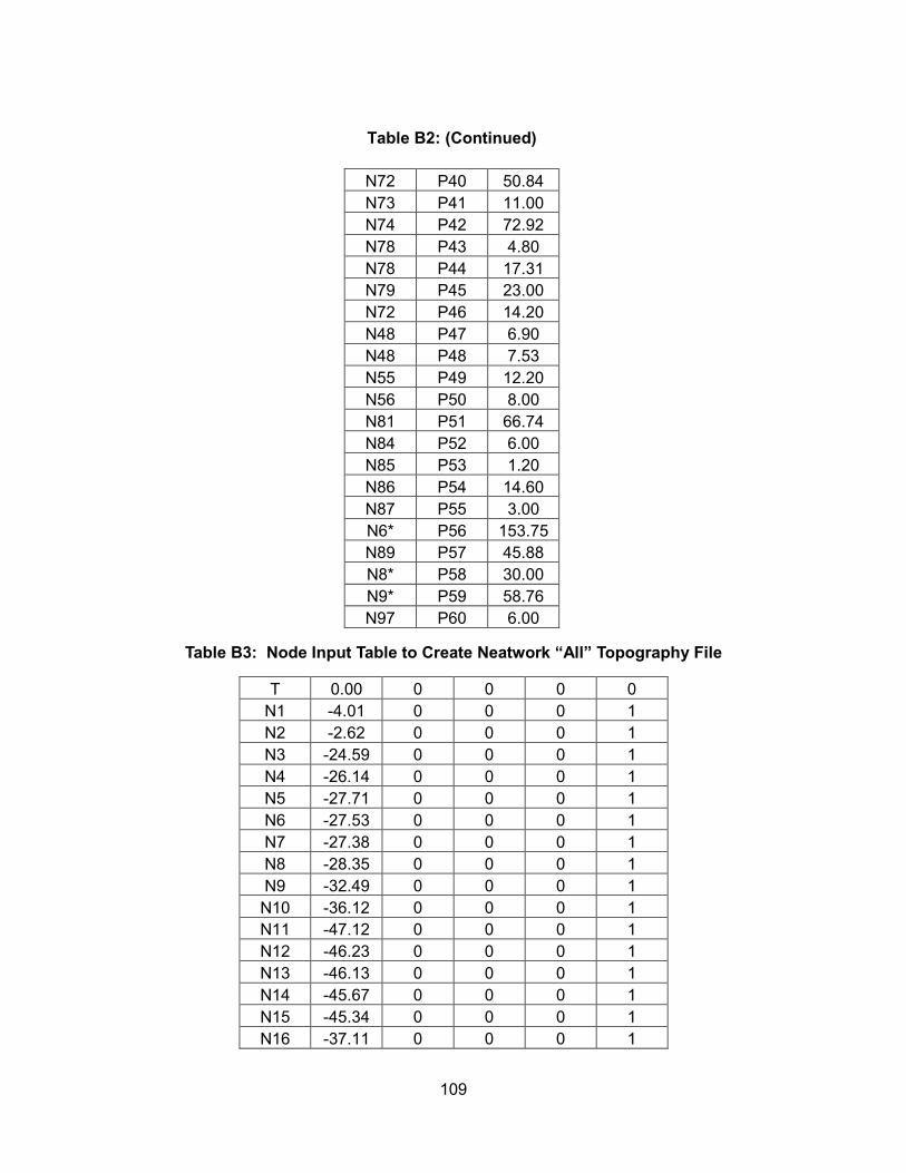
109
Table B2: (Continued)
N72 P40 50.84
N73 P41 11.00
N74 P42 72.92
N78 P43 4.80
N78 P44 17.31
N79 P45 23.00
N72 P46 14.20
N48 P47 6.90
N48 P48 7.53
N55 P49 12.20
N56 P50 8.00
N81 P51 66.74
N84 P52 6.00
N85 P53 1.20
N86 P54 14.60
N87 P55 3.00
N6* P56 153.75
N89 P57 45.88
N8* P58 30.00
N9* P59 58.76
N97 P60 6.00
Table B3: Node Input Table to Create Neatwork “All” Topography File
T 0.00 0 0 0 0
N1 -4.01 0 0 0 1
N2 -2.62 0 0 0 1
N3 -24.59 0 0 0 1
N4 -26.14 0 0 0 1
N5 -27.71 0 0 0 1
N6 -27.53 0 0 0 1
N7 -27.38 0 0 0 1
N8 -28.35 0 0 0 1
N9 -32.49 0 0 0 1
N10 -36.12 0 0 0 1
N11 -47.12 0 0 0 1
N12 -46.23 0 0 0 1
N13 -46.13 0 0 0 1
N14 -45.67 0 0 0 1
N15 -45.34 0 0 0 1
N16 -37.11 0 0 0 1

110
Table B3: (Continued)
N17 -33.78 0 0 0 1
N18 -27.25 0 0 0 1
N19 -26.09 0 0 0 1
N20 -45.72 0 0 0 1
N21 -36.68 0 0 0 1
N22 -31.90 0 0 0 1
N23 -46.15 0 0 0 1
N24 -46.71 0 0 0 1
N25 -27.89 0 0 0 1
N26 -27.89 0 0 0 1
N27 -33.58 0 0 0 1
N28 -36.88 0 0 0 1
N29 -38.35 0 0 0 1
N30 -38.86 0 0 0 1
N31 -37.13 0 0 0 1
N32 -49.48 0 0 0 1
N33 -29.26 0 0 0 1
N34 -29.08 0 0 0 1
N35 -25.76 0 0 0 1
N36 -22.63 0 0 0 1
N37* -30.94 0 0 0 1
N38 -22.68 0 0 0 1
N39 -23.88 0 0 0 1
N40 -17.68 0 0 0 1
N41 -22.96 0 0 0 1
N42 -20.78 0 0 0 1
N43 -39.22 0 0 0 1
N44 -40.41 0 0 0 1
N45 -55.37 0 0 0 1
N46 -48.29 0 0 0 1
N47 -47.60 0 0 0 1
N48 -48.34 0 0 0 1
N49 -52.65 0 0 0 1
N50 -54.48 0 0 0 1
N51 -51.26 0 0 0 1
N52 -51.46 0 0 0 1
N53 -50.09 0 0 0 1
N54 -49.86 0 0 0 1
N55 -49.66 0 0 0 1
N56 -40.11 0 0 0 1
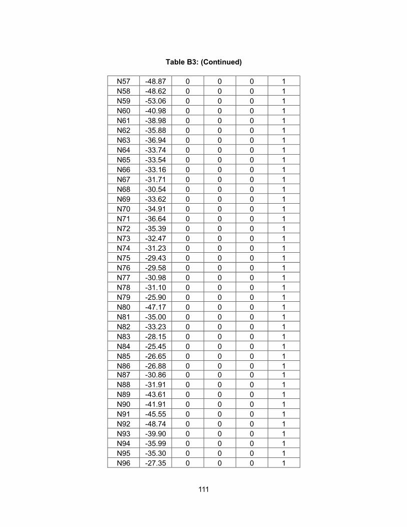
111
Table B3: (Continued)
N57 -48.87 0 0 0 1
N58 -48.62 0 0 0 1
N59 -53.06 0 0 0 1
N60 -40.98 0 0 0 1
N61 -38.98 0 0 0 1
N62 -35.88 0 0 0 1
N63 -36.94 0 0 0 1
N64 -33.74 0 0 0 1
N65 -33.54 0 0 0 1
N66 -33.16 0 0 0 1
N67 -31.71 0 0 0 1
N68 -30.54 0 0 0 1
N69 -33.62 0 0 0 1
N70 -34.91 0 0 0 1
N71 -36.64 0 0 0 1
N72 -35.39 0 0 0 1
N73 -32.47 0 0 0 1
N74 -31.23 0 0 0 1
N75 -29.43 0 0 0 1
N76 -29.58 0 0 0 1
N77 -30.98 0 0 0 1
N78 -31.10 0 0 0 1
N79 -25.90 0 0 0 1
N80 -47.17 0 0 0 1
N81 -35.00 0 0 0 1
N82 -33.23 0 0 0 1
N83 -28.15 0 0 0 1
N84 -25.45 0 0 0 1
N85 -26.65 0 0 0 1
N86 -26.88 0 0 0 1 N87 -30.86 0 0 0 1
N88 -31.91 0 0 0 1
N89 -43.61 0 0 0 1
N90 -41.91 0 0 0 1
N91 -45.55 0 0 0 1
N92 -48.74 0 0 0 1
N93 -39.90 0 0 0 1
N94 -35.99 0 0 0 1
N95 -35.30 0 0 0 1
N96 -27.35 0 0 0 1

112
Table B3: (Continued)
N97 -27.43 0 0 0 1
N1* -45.80 0 0 0 1
N2* -25.86 0 0 0 1
N3* -20.35 0 0 0 1
N4* -22.50 0 0 0 1
N6* -41.68 0 0 0 1
N7* -40.11 0 0 0 1
N8* -38.23 0 0 0 1
N9* -45.04 0 0 0 1
N5* -48.29 0 0 0 2
P1 -27.79 0 0 1 2
PN1 -29.79 0 0 1 2
P2 -29.34 0 0 1 2
P3 -32.92 0 0 1 2
P4 -32.44 0 0 1 2
P5 -36.12 0 0 1 2
P6 -46.36 0 0 1 2
P7 -46.10 0 0 1 2
P8 -43.92 0 0 1 2
P9 -34.57 0 0 1 2
P10 -35.48 0 0 1 2
P11 -26.04 0 0 1 2
P12 -23.19 0 0 1 2
P13 -20.85 0 0 1 2
P14 -20.09 0 0 1 2
P15 -31.09 0 0 1 2
P16 -29.49 0 0 1 2
P17 -44.78 0 0 1 2
P18 -45.92 0 0 1 2
P19 -46.02 0 0 1 2
PN2 -47.68 0 0 1 2
P20 -27.89 0 0 1 2
PN3 -35.94 0 0 1 2
P21 -31.37 0 0 1 2
P22 -35.53 0 0 1 2
P23 -29.87 0 0 1 2
P24 -22.38 0 0 1 2
P25 -23.06 0 0 1 2
P26 -17.32 0 0 1 2
P27 -19.05 0 0 1 2
PN4 -23.80 0 0 1 2

113
Table B3: (Continued)
P28 -18.01 0 0 1 2
P29 -19.81 0 0 1 2
P30 -48.31 0 0 1 2
P31 -48.62 0 0 1 2
P32 -40.98 0 0 1 2
P33 -38.57 0 0 1 2
P34 -36.74 0 0 1 2
P35 -34.58 0 0 1 2
P36 -34.23 0 0 1 2
P37 -30.24 0 0 1 2
PN5 -30.24 0 0 1 2
P38 -35.70 0 0 1 2
P39 -35.29 0 0 1 2
P40 -36.79 0 0 1 2
P41 -33.69 0 0 1 2
P42 -39.03 0 0 1 2
P43 -31.92 0 0 1 2
P44 -25.18 0 0 1 2
P45 -22.21 0 0 1 2
PN6 -25.64 0 0 1 2
P46 -47.45 0 0 1 2
P47 -48.34 0 0 1 2
P48 -48.36 0 0 1 2
PN7 -50.09 0 0 1 2
PN8 -49.79 0 0 1 2
P49 -49.25 0 0 1 2
P50 -40.49 0 0 1 2
P51 -17.07 0 0 1 2
PN9 -33.84 0 0 1 2
PN10 -24.69 0 0 1 2
P52 -25.40 0 0 1 2
P53 -26.52 0 0 1 2
P54 -31.30 0 0 1 2
P55 -30.81 0 0 1 2
P56 -15.47 0 0 1 2
P57 -36.38 0 0 1 2
P58 -42.23 0 0 1 2
P59 -44.15 0 0 1 2
PN11 -40.43 0 0 1 2
PN12 -28.88 0 0 1 2

114
Table B3: (Continued)
P60 -27.48 0 0 1 2
PN13 -27.56 0 0 1 2
Table B4: Arc Length Input Table to Create Neatwork “All” Topography File
T N1 14.85
N1 N2 17.20
N2 N3 93.54
N3 N4 12.20
N4 N5 24.40
N5 N6 11.60
N6 N7 6.70
N7 N8 22.10
N8 N9 42.70
N9 N10 25.77
N10 N11 100.76
N11 N12 48.80
N12 N13 12.20
N13 N14 15.00
N14 N15 6.10
N15 N16 38.92
N16 N17 21.49
N17 N18 30.50
N18 N19 18.30
N12 N20 37.48
N20 N21 30.01
N21 N22 23.38
N12 N23 32.61
N23 N24 33.85
N8 N25 12.20
N25 N26 33.43
N26 N27 48.80
N27 N28 5.00
N28 N29 42.85
N29 N30 4.50
N30 N31 7.80
N31 N32 34.08
N32 N33 59.35
N33 N34 6.10
N34 N35 20.70

115
Table B4: (Continued)
N35 N36 35.90
N36 N37* 36.25
N36 N38 1.55
N38 N39 10.07
N39 N40 103.24
N35 N41 48.80
N29 N30 4.50
N30 N31 7.80
N31 N32 34.08
N32 N33 59.35
N33 N34 6.10
N34 N35 20.70
N35 N36 35.90
N36 N37* 36.25
N36 N38 1.55
N38 N39 10.07
N39 N40 103.24
N35 N41 48.80
N41 N42 42.70
N30 N43 2.30
N43 N44 18.30
N44 N45 16.08
N45 N46 37.20
N46 N47 30.50
N47 N48 40.00
N48 N49 50.00
N49 N50 4.20
N50 N51 139.00
N51 N52 21.35
N52 N53 18.30
N53 N54 18.30
N54 N55 6.10
N55 N56 79.85
N46 N57 12.20
N57 N58 18.70
N58 N59 49.10
N59 N60 52.55
N60 N61 21.35
N61 N62 29.95
N62 N63 8.53
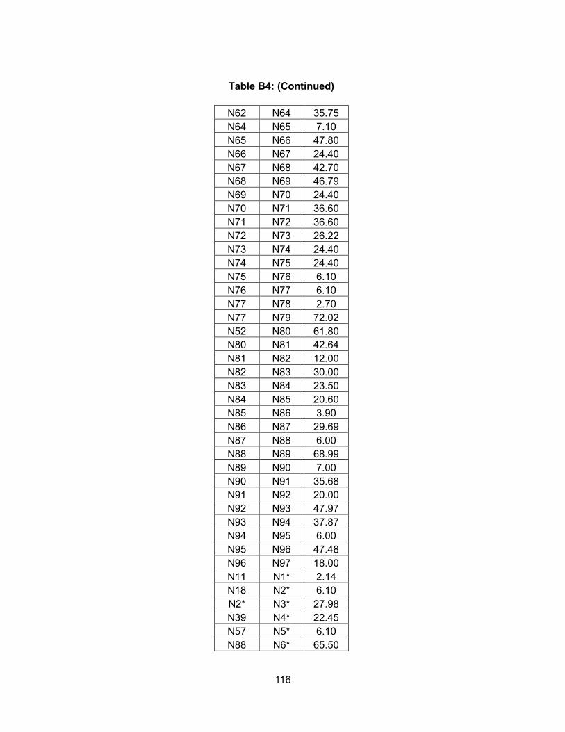
116
Table B4: (Continued)
N62 N64 35.75
N64 N65 7.10
N65 N66 47.80
N66 N67 24.40
N67 N68 42.70
N68 N69 46.79
N69 N70 24.40
N70 N71 36.60
N71 N72 36.60
N72 N73 26.22
N73 N74 24.40
N74 N75 24.40
N75 N76 6.10
N76 N77 6.10
N77 N78 2.70
N77 N79 72.02
N52 N80 61.80
N80 N81 42.64
N81 N82 12.00
N82 N83 30.00
N83 N84 23.50
N84 N85 20.60
N85 N86 3.90
N86 N87 29.69
N87 N88 6.00
N88 N89 68.99
N89 N90 7.00
N90 N91 35.68
N91 N92 20.00
N92 N93 47.97
N93 N94 37.87
N94 N95 6.00
N95 N96 47.48
N96 N97 18.00
N11 N1* 2.14
N18 N2* 6.10
N2* N3* 27.98
N39 N4* 22.45
N57 N5* 6.10
N88 N6* 65.50

117
Table B4: (Continued)
N91 N7* 10.95
N7* N8* 24.00
N92 N9* 8.00
N3 P1 19.37
N5 P2 9.63
N6 P3 145.67
N9 P4 18.30
N10 P5 0.50
N1* P6 8.64
N13 P7 11.80
N14 P8 19.83
N16 P9 17.25
N17 P10 34.30
N19 P11 12.20
N19 P12 36.60
N3* P13 6.10
N22 P14 55.00
N22 P15 2.70
N22 P16 26.88
N23 P17 18.30
N24 P18 18.30
N24 P19 14.87
N26 P20 0.80
N37* P21 2.50
N37* P22 35.53
N34 P23 30.50
N38 P24 4.78
N4* P25 31.75
N40 P26 0.50
N40 P27 35.50
N42 P28 42.70
N42 P29 20.85
N57 P30 24.87
N58 P31 0.50
N60 P32 0.50
N62 P33 64.58
N63 P34 4.50
N64 P35 13.00
N66 P36 26.27

118
Table B4: (Continued)
N67 P37 35.90
N69 P38 28.70
N70 P39 6.10
N72 P40 50.84
N73 P41 11.00
N74 P42 72.92
N78 P43 4.80
N78 P44 17.31
N79 P45 23.00
N72 P46 14.20
N48 P47 6.90
N48 P48 7.53
N55 P49 12.20
N56 P50 8.00
N81 P51 66.74
N84 P52 6.00
N85 P53 1.20
N86 P54 14.60
N87 P55 3.00
N6* P56 153.75
N89 P57 45.88
N8* P58 30.00
N9* P59 58.76
N97 P60 6.00
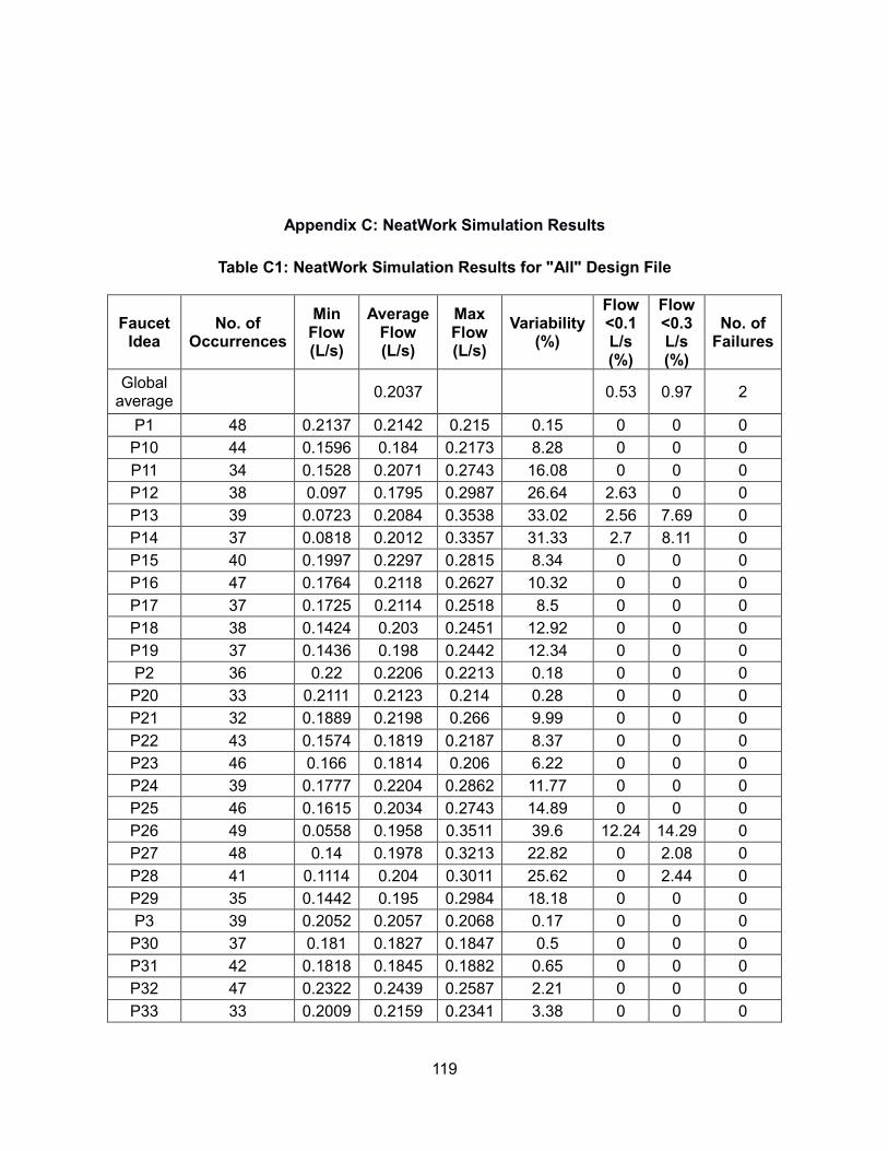
119
Appendix C: NeatWork Simulation Results
Table C1: NeatWork Simulation Results for "All" Design File
Faucet Idea
No. of Occurrences
Min Flow (L/s)
Average Flow (L/s)
Max Flow (L/s)
Variability (%)
Flow <0.1 L/s (%)
Flow <0.3 L/s (%)
No. of Failures
Global average
0.2037 0.53 0.97 2
P1 48 0.2137 0.2142 0.215 0.15 0 0 0
P10 44 0.1596 0.184 0.2173 8.28 0 0 0
P11 34 0.1528 0.2071 0.2743 16.08 0 0 0
P12 38 0.097 0.1795 0.2987 26.64 2.63 0 0
P13 39 0.0723 0.2084 0.3538 33.02 2.56 7.69 0
P14 37 0.0818 0.2012 0.3357 31.33 2.7 8.11 0
P15 40 0.1997 0.2297 0.2815 8.34 0 0 0
P16 47 0.1764 0.2118 0.2627 10.32 0 0 0
P17 37 0.1725 0.2114 0.2518 8.5 0 0 0
P18 38 0.1424 0.203 0.2451 12.92 0 0 0
P19 37 0.1436 0.198 0.2442 12.34 0 0 0
P2 36 0.22 0.2206 0.2213 0.18 0 0 0
P20 33 0.2111 0.2123 0.214 0.28 0 0 0
P21 32 0.1889 0.2198 0.266 9.99 0 0 0
P22 43 0.1574 0.1819 0.2187 8.37 0 0 0
P23 46 0.166 0.1814 0.206 6.22 0 0 0
P24 39 0.1777 0.2204 0.2862 11.77 0 0 0
P25 46 0.1615 0.2034 0.2743 14.89 0 0 0
P26 49 0.0558 0.1958 0.3511 39.6 12.24 14.29 0
P27 48 0.14 0.1978 0.3213 22.82 0 2.08 0
P28 41 0.1114 0.204 0.3011 25.62 0 2.44 0
P29 35 0.1442 0.195 0.2984 18.18 0 0 0
P3 39 0.2052 0.2057 0.2068 0.17 0 0 0
P30 37 0.181 0.1827 0.1847 0.5 0 0 0
P31 42 0.1818 0.1845 0.1882 0.65 0 0 0
P32 47 0.2322 0.2439 0.2587 2.21 0 0 0
P33 33 0.2009 0.2159 0.2341 3.38 0 0 0

120
Table C1: (Continued)
P34 47 0.2039 0.2183 0.2306 2.65 0 0 0
P35 43 0.1903 0.2068 0.2213 3.33 0 0 0
P36 41 0.1813 0.2027 0.2228 4.44 0 0 0
P37 39 0.1632 0.1802 0.2041 5.05 0 0 0
P38 44 0.1814 0.2012 0.2278 4.34 0 0 0
P39 39 0.1787 0.1984 0.2146 5.07 0 0 0
P4 47 0.2216 0.2244 0.2271 0.58 0 0 0
P40 35 0.1602 0.183 0.2158 7.17 0 0 0
P41 39 0.1965 0.2288 0.2649 8.1 0 0 0
P42 35 0.1617 0.1814 0.2271 7.96 0 0 0
P43 37 0.1748 0.2066 0.2469 8.73 0 0 0
P44 37 0.1213 0.2007 0.3015 23.93 0 2.7 0
P45 42 0.0 0.22 0.3659 39.11 4.76 21.43 2
P46 35 0.2178 0.2335 0.2631 4.67 0 0 0
P47 44 0.1816 0.1836 0.1857 0.54 0 0 0
P48 40 0.1816 0.1835 0.1859 0.56 0 0 0
P49 36 0.1498 0.1685 0.1806 5.22 0 0 0
P5 45 0.2374 0.2411 0.2458 0.81 0 0 0
P50 36 0.1734 0.2002 0.2198 6.15 0 0 0
P51 35 0.1335 0.1799 0.2194 9.45 0 0 0
P52 44 0.1886 0.2181 0.2451 5.92 0 0 0
P53 52 0.1973 0.2271 0.2557 5.1 0 0 0
P54 53 0.169 0.1878 0.2065 3.95 0 0 0
P55 40 0.167 0.1863 0.2044 4.22 0 0 0
P56 40 0.0535 0.2001 0.2694 24.43 2.5 0 0
P57 39 0.1655 0.1936 0.2202 5.73 0 0 0
P58 42 0.18 0.207 0.2318 5.35 0 0 0
P59 44 0.1854 0.2128 0.2348 5.38 0 0 0
P6 37 0.1666 0.1725 0.1805 1.99 0 0 0
P60 39 0.0865 0.2002 0.2931 29.1 10.26 0 0
P7 44 0.2203 0.2383 0.2655 4.53 0 0 0
P8 37 0.2072 0.2257 0.2564 4.8 0 0 0
P9 38 0.1584 0.1868 0.2201 8.51 0 0 0
PN1 46 0.2227 0.2232 0.2242 0.16 0 0 0
PN10 35 0.1852 0.2108 0.2353 5.63 0 0 0
PN11 32 0.1752 0.2043 0.2428 6.86 0 0 0
PN12 47 0.1403 0.221 0.284 14.69 0 0 0
PN13 31 0.1084 0.2099 0.3316 28.56 0 6.45 0
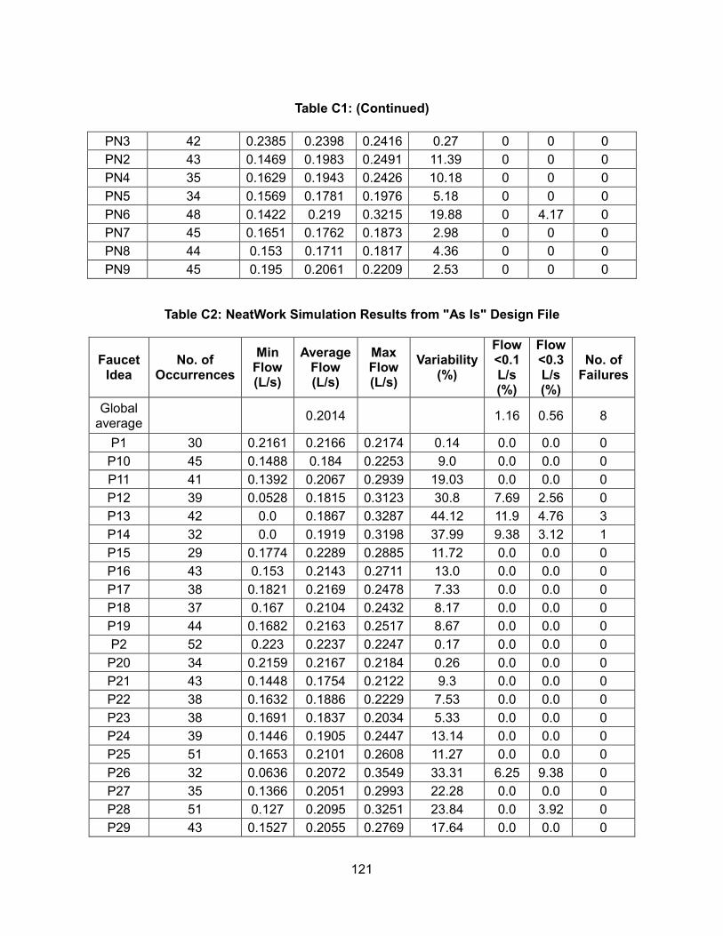
121
Table C1: (Continued)
PN3 42 0.2385 0.2398 0.2416 0.27 0 0 0
PN2 43 0.1469 0.1983 0.2491 11.39 0 0 0
PN4 35 0.1629 0.1943 0.2426 10.18 0 0 0
PN5 34 0.1569 0.1781 0.1976 5.18 0 0 0
PN6 48 0.1422 0.219 0.3215 19.88 0 4.17 0
PN7 45 0.1651 0.1762 0.1873 2.98 0 0 0
PN8 44 0.153 0.1711 0.1817 4.36 0 0 0
PN9 45 0.195 0.2061 0.2209 2.53 0 0 0
Table C2: NeatWork Simulation Results from "As Is" Design File
Faucet Idea
No. of Occurrences
Min Flow (L/s)
Average Flow (L/s)
Max Flow (L/s)
Variability (%)
Flow <0.1 L/s (%)
Flow <0.3 L/s (%)
No. of Failures
Global average
0.2014 1.16 0.56 8
P1 30 0.2161 0.2166 0.2174 0.14 0.0 0.0 0
P10 45 0.1488 0.184 0.2253 9.0 0.0 0.0 0
P11 41 0.1392 0.2067 0.2939 19.03 0.0 0.0 0
P12 39 0.0528 0.1815 0.3123 30.8 7.69 2.56 0
P13 42 0.0 0.1867 0.3287 44.12 11.9 4.76 3
P14 32 0.0 0.1919 0.3198 37.99 9.38 3.12 1
P15 29 0.1774 0.2289 0.2885 11.72 0.0 0.0 0
P16 43 0.153 0.2143 0.2711 13.0 0.0 0.0 0
P17 38 0.1821 0.2169 0.2478 7.33 0.0 0.0 0
P18 37 0.167 0.2104 0.2432 8.17 0.0 0.0 0
P19 44 0.1682 0.2163 0.2517 8.67 0.0 0.0 0
P2 52 0.223 0.2237 0.2247 0.17 0.0 0.0 0
P20 34 0.2159 0.2167 0.2184 0.26 0.0 0.0 0
P21 43 0.1448 0.1754 0.2122 9.3 0.0 0.0 0
P22 38 0.1632 0.1886 0.2229 7.53 0.0 0.0 0
P23 38 0.1691 0.1837 0.2034 5.33 0.0 0.0 0
P24 39 0.1446 0.1905 0.2447 13.14 0.0 0.0 0
P25 51 0.1653 0.2101 0.2608 11.27 0.0 0.0 0
P26 32 0.0636 0.2072 0.3549 33.31 6.25 9.38 0
P27 35 0.1366 0.2051 0.2993 22.28 0.0 0.0 0
P28 51 0.127 0.2095 0.3251 23.84 0.0 3.92 0
P29 43 0.1527 0.2055 0.2769 17.64 0.0 0.0 0

122
Table C2: (Continued)
P3 44 0.2079 0.2085 0.2096 0.17 0.0 0.0 0
P30 43 0.1781 0.1808 0.1846 0.72 0.0 0.0 0
P31 36 0.1796 0.183 0.1879 0.88 0.0 0.0 0
P32 42 0.2337 0.2426 0.2546 1.91 0.0 0.0 0
P33 37 0.2044 0.2156 0.2292 2.81 0.0 0.0 0
P34 40 0.2077 0.2193 0.2338 2.62 0.0 0.0 0
P35 41 0.1956 0.2082 0.2227 3.05 0.0 0.0 0
P36 50 0.1885 0.2021 0.2166 3.24 0.0 0.0 0
P37 42 0.167 0.1805 0.2016 4.68 0.0 0.0 0
P38 46 0.1765 0.1925 0.2176 4.85 0.0 0.0 0
P39 35 0.1745 0.191 0.2142 5.51 0.0 0.0 0
P4 40 0.2261 0.2286 0.2318 0.52 0.0 0.0 0
P40 37 0.1529 0.1814 0.2216 9.45 0.0 0.0 0
P41 47 0.1853 0.2247 0.2818 10.09 0.0 0.0 0
P42 43 0.1554 0.1791 0.2124 7.56 0.0 0.0 0
P43 44 0.1629 0.2037 0.2769 11.9 0.0 0.0 0
P44 37 0.0818 0.1777 0.2634 20.49 2.7 0.0 0
P45 44 0.0 0.1781 0.3361 51.55 20.45 9.09 3
P46 47 0.2111 0.2298 0.2558 4.5 0.0 0.0 0
P47 51 0.1771 0.1807 0.186 1.06 0.0 0.0 0
P48 41 0.1771 0.1809 0.1868 1.26 0.0 0.0 0
P49 39 0.1559 0.1686 0.1857 4.16 0.0 0.0 0
P5 41 0.2415 0.2451 0.2494 0.6 0.0 0.0 0
P50 37 0.1838 0.2024 0.2208 4.83 0.0 0.0 0
P51 41 0.1315 0.2046 0.2849 16.95 0.0 0.0 0
P52 42 0.1855 0.2118 0.249 7.73 0.0 0.0 0
P53 43 0.1978 0.225 0.2653 7.04 0.0 0.0 0
P54 39 0.1685 0.1862 0.2111 5.82 0.0 0.0 0
P55 37 0.1675 0.1843 0.2033 5.34 0.0 0.0 0
P56 44 0.0 0.187 0.3358 38.19 13.64 2.27 1
P57 42 0.1779 0.1962 0.2221 5.97 0.0 0.0 0
P58 46 0.1842 0.2069 0.237 5.88 0.0 0.0 0
P59 44 0.1832 0.2081 0.2362 6.89 0.0 0.0 0
P6 40 0.1601 0.1721 0.1845 3.18 0.0 0.0 0
P60 35 0.1244 0.1939 0.2668 18.06 0.0 0.0 0
P7 32 0.2105 0.24 0.2619 5.04 0.0 0.0 0
P8 49 0.1974 0.2286 0.2581 5.76 0.0 0.0 0
P9 40 0.1468 0.1811 0.2159 8.14 0.0 0.0 0
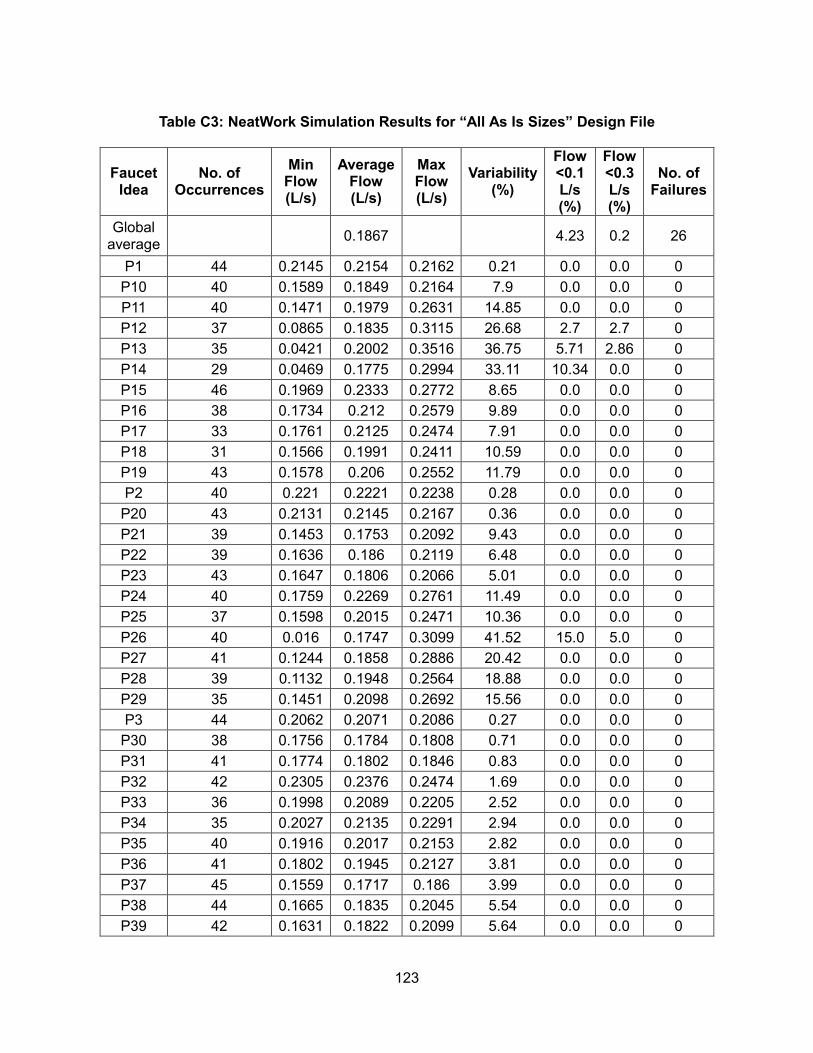
123
Table C3: NeatWork Simulation Results for “All As Is Sizes” Design File
Faucet Idea
No. of Occurrences
Min Flow (L/s)
Average Flow (L/s)
Max Flow (L/s)
Variability (%)
Flow <0.1 L/s (%)
Flow <0.3 L/s (%)
No. of Failures
Global average
0.1867 4.23 0.2 26
P1 44 0.2145 0.2154 0.2162 0.21 0.0 0.0 0
P10 40 0.1589 0.1849 0.2164 7.9 0.0 0.0 0
P11 40 0.1471 0.1979 0.2631 14.85 0.0 0.0 0
P12 37 0.0865 0.1835 0.3115 26.68 2.7 2.7 0
P13 35 0.0421 0.2002 0.3516 36.75 5.71 2.86 0
P14 29 0.0469 0.1775 0.2994 33.11 10.34 0.0 0
P15 46 0.1969 0.2333 0.2772 8.65 0.0 0.0 0
P16 38 0.1734 0.212 0.2579 9.89 0.0 0.0 0
P17 33 0.1761 0.2125 0.2474 7.91 0.0 0.0 0
P18 31 0.1566 0.1991 0.2411 10.59 0.0 0.0 0
P19 43 0.1578 0.206 0.2552 11.79 0.0 0.0 0
P2 40 0.221 0.2221 0.2238 0.28 0.0 0.0 0
P20 43 0.2131 0.2145 0.2167 0.36 0.0 0.0 0
P21 39 0.1453 0.1753 0.2092 9.43 0.0 0.0 0
P22 39 0.1636 0.186 0.2119 6.48 0.0 0.0 0
P23 43 0.1647 0.1806 0.2066 5.01 0.0 0.0 0
P24 40 0.1759 0.2269 0.2761 11.49 0.0 0.0 0
P25 37 0.1598 0.2015 0.2471 10.36 0.0 0.0 0
P26 40 0.016 0.1747 0.3099 41.52 15.0 5.0 0
P27 41 0.1244 0.1858 0.2886 20.42 0.0 0.0 0
P28 39 0.1132 0.1948 0.2564 18.88 0.0 0.0 0
P29 35 0.1451 0.2098 0.2692 15.56 0.0 0.0 0
P3 44 0.2062 0.2071 0.2086 0.27 0.0 0.0 0
P30 38 0.1756 0.1784 0.1808 0.71 0.0 0.0 0
P31 41 0.1774 0.1802 0.1846 0.83 0.0 0.0 0
P32 42 0.2305 0.2376 0.2474 1.69 0.0 0.0 0
P33 36 0.1998 0.2089 0.2205 2.52 0.0 0.0 0
P34 35 0.2027 0.2135 0.2291 2.94 0.0 0.0 0
P35 40 0.1916 0.2017 0.2153 2.82 0.0 0.0 0
P36 41 0.1802 0.1945 0.2127 3.81 0.0 0.0 0
P37 45 0.1559 0.1717 0.186 3.99 0.0 0.0 0
P38 44 0.1665 0.1835 0.2045 5.54 0.0 0.0 0
P39 42 0.1631 0.1822 0.2099 5.64 0.0 0.0 0

124
Table C3: (Continued)
P4 46 0.2236 0.2265 0.2294 0.61 0.0 0.0 0
P40 41 0.1489 0.1719 0.2082 7.66 0.0 0.0 0
P41 33 0.175 0.2046 0.2524 8.19 0.0 0.0 0
P42 39 0.1498 0.175 0.2016 7.0 0.0 0.0 0
P43 40 0.1524 0.193 0.2699 11.51 0.0 0.0 0
P44 42 0.0161 0.1674 0.2731 30.72 7.14 0.0 0
P45 48 0.0 0.1265 0.4067 82.77 43.75 4.17 10
P46 45 0.2061 0.2241 0.2458 4.9 0.0 0.0 0
P47 51 0.173 0.1767 0.1798 0.8 0.0 0.0 0
P48 36 0.173 0.1766 0.1799 0.93 0.0 0.0 0
P49 42 0.1376 0.1563 0.1682 5.5 0.0 0.0 0
P5 39 0.2396 0.2429 0.2474 0.66 0.0 0.0 0
P50 43 0.1522 0.1828 0.2074 7.9 0.0 0.0 0
P51 38 0.0 0.1299 0.2136 40.99 28.95 0.0 1
P52 35 0.1418 0.1845 0.2166 8.35 0.0 0.0 0
P53 42 0.1747 0.1968 0.2273 6.89 0.0 0.0 0
P54 41 0.1443 0.1699 0.1866 5.31 0.0 0.0 0
P55 44 0.1422 0.168 0.1884 5.66 0.0 0.0 0
P56 47 0.0 0.0744 0.1801 84.92 55.32 0.0 14
P57 46 0.1588 0.1791 0.1974 4.63 0.0 0.0 0
P58 38 0.1746 0.1902 0.2143 5.21 0.0 0.0 0
P59 49 0.172 0.1905 0.2166 6.13 0.0 0.0 0
P6 46 0.1633 0.1711 0.1843 2.43 0.0 0.0 0
P60 33 0.0 0.0961 0.1999 47.98 57.58 0.0 1
P7 32 0.218 0.2355 0.2616 4.6 0.0 0.0 0
P8 45 0.2055 0.2264 0.2547 5.3 0.0 0.0 0
P9 36 0.1589 0.1868 0.2289 9.33 0.0 0.0 0
PN1 36 0.2235 0.2244 0.2257 0.21 0.0 0.0 0
PN10 45 0.1346 0.1807 0.2202 8.9 0.0 0.0 0
PN11 37 0.1506 0.1716 0.2052 7.85 0.0 0.0 0
PN12 38 0.0521 0.1128 0.2139 24.52 31.58 0.0 0
PN13 36 0.0153 0.0976 0.1997 50.6 61.11 0.0 0
PN2 29 0.1599 0.1988 0.2314 9.59 0.0 0.0 0
PN3 44 0.2407 0.2418 0.2434 0.26 0.0 0.0 0
PN4 40 0.1631 0.1955 0.2351 8.9 0.0 0.0 0
PN5 45 0.1512 0.1685 0.1949 4.83 0.0 0.0 0
PN6 40 0.0644 0.1823 0.2917 25.64 2.5 0.0 0
PN7 47 0.1519 0.1652 0.1755 3.6 0.0 0.0 0
PN8 49 0.1408 0.1591 0.1741 5.46 0.0 0.0 0
PN9 52 0.1655 0.1877 0.208 4.4 0.0 0.0 0

125
Table C4: NeatWork Simulation Results for “All As Is Sizes No Discs” Design File
Faucet Idea
No. of Occurrences
Min Flow (L/s)
Average Flow (L/s)
Max Flow (L/s)
Variability (%)
Flow <0.1 L/s (%)
Flow <0.3 L/s (%)
No. of Failures
Global average
0.2082 7.57 11.47 120
P1 39 0.2115 0.2141 0.2158 0.48 0.0 0.0 0
P10 38 0.1419 0.1791 0.2204 9.48 0.0 0.0 0
P11 40 0.1011 0.1991 0.2873 18.19 0.0 0.0 0
P12 40 0.0 0.1626 0.2695 29.52 2.5 0.0 1
P13 33 0.0 0.1663 0.3273 43.89 12.12 3.03 1
P14 48 0.0 0.1698 0.273 40.67 16.67 0.0 1
P15 39 0.1685 0.2263 0.2852 11.34 0.0 0.0 0
P16 35 0.1436 0.1997 0.2558 11.75 0.0 0.0 0
P17 46 0.1521 0.195 0.2481 13.41 0.0 0.0 0
P18 42 0.106 0.1753 0.233 22.79 0.0 0.0 0
P19 36 0.1073 0.1767 0.2427 23.42 0.0 0.0 0
P2 38 0.2173 0.2202 0.2225 0.59 0.0 0.0 0
P20 48 0.2077 0.2117 0.2144 0.84 0.0 0.0 0
P21 40 0.1397 0.1647 0.1876 7.85 0.0 0.0 0
P22 46 0.1589 0.1801 0.208 6.52 0.0 0.0 0
P23 35 0.1593 0.1721 0.1979 5.27 0.0 0.0 0
P24 47 0.1657 0.2096 0.2696 13.07 0.0 0.0 0
P25 41 0.152 0.1867 0.2529 12.28 0.0 0.0 0
P26 38 0.0 0.1541 0.3065 52.23 23.68 2.63 2
P27 37 0.1079 0.1709 0.2622 21.65 0.0 0.0 0
P28 48 0.0259 0.1579 0.2799 36.73 20.83 0.0 0
P3 44 0.2029 0.2053 0.2075 0.54 0.0 0.0 0
P30 43 0.1705 0.1746 0.1791 1.08 0.0 0.0 0
P31 45 0.1726 0.1767 0.1817 1.17 0.0 0.0 0
P32 45 0.2196 0.2311 0.2431 2.17 0.0 0.0 0
P33 36 0.189 0.2041 0.2162 3.32 0.0 0.0 0
P34 36 0.191 0.206 0.2226 3.17 0.0 0.0 0
P35 44 0.1771 0.1945 0.211 3.53 0.0 0.0 0
P36 43 0.1686 0.1883 0.2054 4.35 0.0 0.0 0
P37 34 0.1448 0.164 0.1794 5.26 0.0 0.0 0
P38 35 0.1528 0.1782 0.2011 6.34 0.0 0.0 0
P39 46 0.1491 0.1753 0.2017 6.67 0.0 0.0 0
P4 28 0.2206 0.2241 0.2272 0.7 0.0 0.0 0

126
Table C4: (Continued)
P40 46 0.1462 0.1664 0.1995 7.58 0.0 0.0 0
P41 36 0.1697 0.2019 0.2587 10.0 0.0 0.0 0
P42 40 0.1487 0.1699 0.1988 7.08 0.0 0.0 0
P43 47 0.1503 0.1815 0.2194 9.35 0.0 0.0 0
P44 42 0.0 0.1613 0.2689 33.49 9.52 0.0 1
P45 34 0.0 0.111 0.277 73.04 41.18 0.0 7
P46 29 0.2018 0.2164 0.2417 3.92 0.0 0.0 0
P47 42 0.1651 0.1719 0.1778 1.6 0.0 0.0 0
P48 45 0.1651 0.1722 0.1775 1.79 0.0 0.0 0
P49 44 0.0844 0.1221 0.1628 17.02 13.64 0.0 0
P5 44 0.2372 0.2412 0.2445 0.72 0.0 0.0 0
P50 55 0.0243 0.1357 0.2094 36.46 12.73 0.0 0
P51 39 0.0 0.0468 0.1899 121.72 82.05 0.0 18
P52 43 0.089 0.1529 0.2065 19.3 4.65 0.0 0
P53 34 0.1084 0.1662 0.2134 15.28 0.0 0.0 0
P54 36 0.1208 0.153 0.1811 9.46 0.0 0.0 0
P55 46 0.1186 0.1513 0.19 11.03 0.0 0.0 0
P56 46 0.0 0.0213 0.1696 212.01 91.3 0.0 34
P57 39 0.1447 0.1628 0.1894 7.01 0.0 0.0 0
P58 43 0.1445 0.1736 0.2102 9.03 0.0 0.0 0
P59 38 0.136 0.1695 0.2086 11.55 0.0 0.0 0
P6 39 0.1581 0.168 0.1796 2.78 0.0 0.0 0
P60 35 0.0 0.0408 0.1499 110.97 88.57 0.0 16
P7 37 0.2061 0.2318 0.2537 4.71 0.0 0.0 0
P8 39 0.1927 0.2205 0.243 4.75 0.0 0.0 0
P9 42 0.1397 0.1795 0.2155 9.24 0.0 0.0 0
PN1 39 0.6575 0.663 0.6674 0.42 0.0 100.0 0
PN2 39 0.2689 0.3542 0.4438 12.34 0.0 92.31 0
PN10 40 0.1652 0.2883 0.4191 21.94 0.0 37.5 0
PN11 47 0.2662 0.3461 0.4693 11.23 0.0 87.23 0
PN12 47 0.0 0.0794 0.2289 104.49 51.06 0.0 24
PN13 38 0.0 0.0547 0.1868 107.89 84.21 0.0 15
PN3 33 0.6986 0.7065 0.7127 0.49 0.0 100.0 0
PN4 42 0.326 0.3723 0.4532 7.0 0.0 100.0 0
PN5 45 0.3821 0.4356 0.5017 5.54 0.0 100.0 0
PN6 34 0.0761 0.2265 0.3947 32.94 2.94 11.76 0
PN7 43 0.5264 0.6173 0.7107 9.92 0.0 100.0 0
PN8 44 0.3908 0.5002 0.6085 13.86 0.0 100.0 0
PN9 38 0.1424 0.1667 0.2009 8.94 0.0 0.0 0
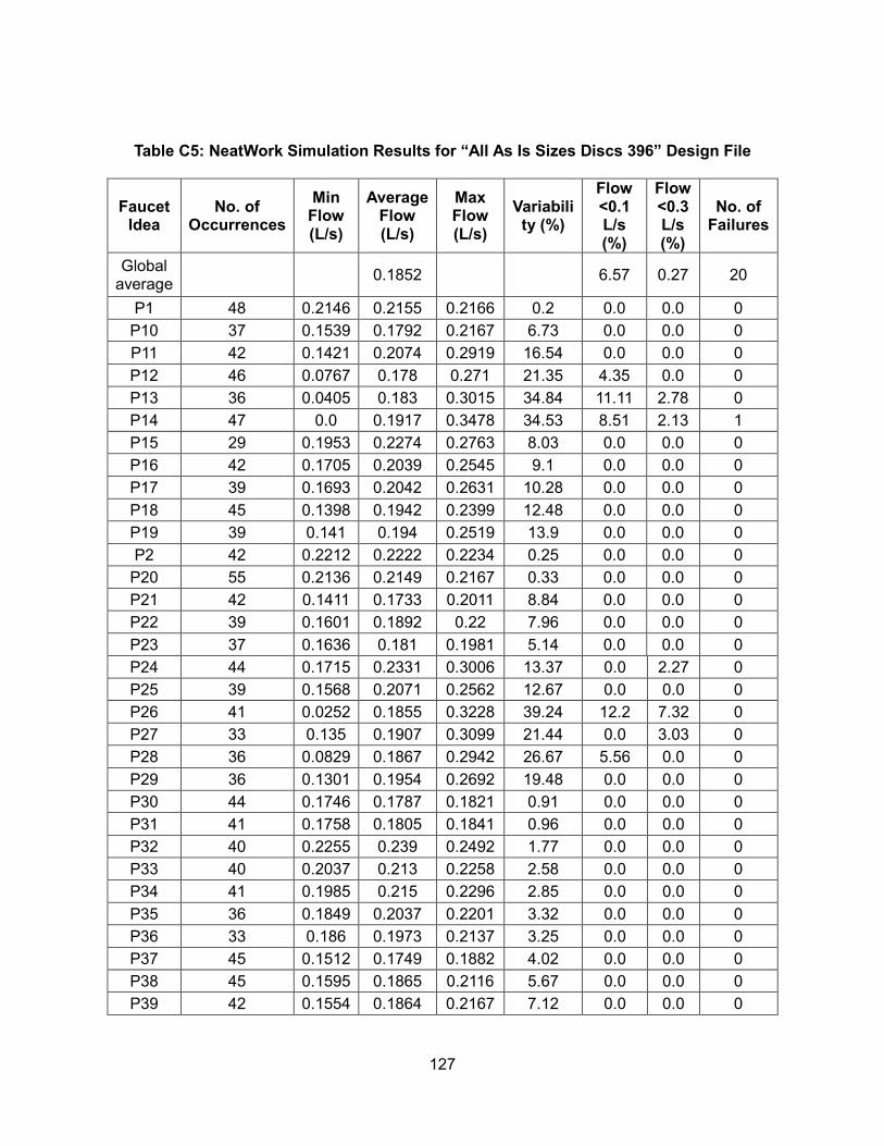
127
Table C5: NeatWork Simulation Results for “All As Is Sizes Discs 396” Design File
Faucet Idea
No. of Occurrences
Min Flow (L/s)
Average Flow (L/s)
Max Flow (L/s)
Variability (%)
Flow <0.1 L/s (%)
Flow <0.3 L/s (%)
No. of Failures
Global average
0.1852 6.57 0.27 20
P1 48 0.2146 0.2155 0.2166 0.2 0.0 0.0 0
P10 37 0.1539 0.1792 0.2167 6.73 0.0 0.0 0
P11 42 0.1421 0.2074 0.2919 16.54 0.0 0.0 0
P12 46 0.0767 0.178 0.271 21.35 4.35 0.0 0
P13 36 0.0405 0.183 0.3015 34.84 11.11 2.78 0
P14 47 0.0 0.1917 0.3478 34.53 8.51 2.13 1
P15 29 0.1953 0.2274 0.2763 8.03 0.0 0.0 0
P16 42 0.1705 0.2039 0.2545 9.1 0.0 0.0 0
P17 39 0.1693 0.2042 0.2631 10.28 0.0 0.0 0
P18 45 0.1398 0.1942 0.2399 12.48 0.0 0.0 0
P19 39 0.141 0.194 0.2519 13.9 0.0 0.0 0
P2 42 0.2212 0.2222 0.2234 0.25 0.0 0.0 0
P20 55 0.2136 0.2149 0.2167 0.33 0.0 0.0 0
P21 42 0.1411 0.1733 0.2011 8.84 0.0 0.0 0
P22 39 0.1601 0.1892 0.22 7.96 0.0 0.0 0
P23 37 0.1636 0.181 0.1981 5.14 0.0 0.0 0
P24 44 0.1715 0.2331 0.3006 13.37 0.0 2.27 0
P25 39 0.1568 0.2071 0.2562 12.67 0.0 0.0 0
P26 41 0.0252 0.1855 0.3228 39.24 12.2 7.32 0
P27 33 0.135 0.1907 0.3099 21.44 0.0 3.03 0
P28 36 0.0829 0.1867 0.2942 26.67 5.56 0.0 0
P29 36 0.1301 0.1954 0.2692 19.48 0.0 0.0 0
P30 44 0.1746 0.1787 0.1821 0.91 0.0 0.0 0
P31 41 0.1758 0.1805 0.1841 0.96 0.0 0.0 0
P32 40 0.2255 0.239 0.2492 1.77 0.0 0.0 0
P33 40 0.2037 0.213 0.2258 2.58 0.0 0.0 0
P34 41 0.1985 0.215 0.2296 2.85 0.0 0.0 0
P35 36 0.1849 0.2037 0.2201 3.32 0.0 0.0 0
P36 33 0.186 0.1973 0.2137 3.25 0.0 0.0 0
P37 45 0.1512 0.1749 0.1882 4.02 0.0 0.0 0
P38 45 0.1595 0.1865 0.2116 5.67 0.0 0.0 0
P39 42 0.1554 0.1864 0.2167 7.12 0.0 0.0 0

128
Table C5: (Continued)
P4 35 0.224 0.2264 0.2302 0.59 0.0 0.0 0
P40 39 0.145 0.1763 0.2068 10.12 0.0 0.0 0
P41 39 0.1855 0.2192 0.261 9.39 0.0 0.0 0
P42 35 0.1525 0.1732 0.2043 7.52 0.0 0.0 0
P43 38 0.1596 0.1994 0.2646 11.83 0.0 0.0 0
P44 39 0.0681 0.1786 0.3195 32.97 12.82 2.56 0
P45 34 0.0 0.0747 0.1487 54.9 73.53 0.0 4
P46 46 0.2051 0.2279 0.258 5.7 0.0 0.0 0
P47 38 0.174 0.1774 0.18 0.92 0.0 0.0 0
P48 44 0.1742 0.1774 0.1813 1.04 0.0 0.0 0
P49 41 0.1282 0.1568 0.1722 6.88 0.0 0.0 0
P5 46 0.24 0.2431 0.2485 0.72 0.0 0.0 0
P50 37 0.1351 0.1818 0.2078 9.17 0.0 0.0 0
P51 40 0.0 0.0661 0.1013 32.67 97.5 0.0 1
P52 43 0.1515 0.1879 0.2186 7.25 0.0 0.0 0
P53 45 0.164 0.2 0.2365 7.78 0.0 0.0 0
P54 50 0.1497 0.1723 0.1887 4.78 0.0 0.0 0
P55 54 0.1525 0.1707 0.1869 4.76 0.0 0.0 0
P56 42 0.0 0.0811 0.2131 86.08 52.38 0.0 13
P57 43 0.1643 0.1824 0.195 4.42 0.0 0.0 0
P58 29 0.1725 0.1898 0.215 5.46 0.0 0.0 0
P59 53 0.1705 0.1891 0.2081 4.63 0.0 0.0 0
P6 37 0.1636 0.1703 0.1796 2.14 0.0 0.0 0
P60 40 0.0 0.1066 0.2301 48.59 55.0 0.0 1
P7 40 0.2151 0.2387 0.2631 4.76 0.0 0.0 0
P8 46 0.202 0.2231 0.2478 4.62 0.0 0.0 0
P9 33 0.1522 0.1769 0.1995 6.78 0.0 0.0 0
PN1 40 0.2236 0.2245 0.2254 0.19 0.0 0.0 0
PN10 48 0.1062 0.1351 0.1522 7.91 0.0 0.0 0
PN11 33 0.1537 0.1666 0.1945 5.51 0.0 0.0 0
PN12 35 0.0474 0.085 0.1454 31.23 74.29 0.0 0
PN13 54 0.0097 0.1016 0.2306 49.24 53.7 0.0 0
PN2 39 0.1446 0.1907 0.2378 10.89 0.0 0.0 0
PN3 28 0.2409 0.2422 0.2438 0.28 0.0 0.0 0
PN4 41 0.1166 0.1465 0.1737 10.14 0.0 0.0 0
PN5 44 0.1453 0.1734 0.1935 5.55 0.0 0.0 0
PN6 36 0.0486 0.1104 0.1732 28.58 33.33 0.0 0
PN7 37 0.2192 0.249 0.2645 4.21 0.0 0.0 0
PN8 25 0.1981 0.2289 0.248 5.08 0.0 0.0 0
PN9 49 0.1697 0.1905 0.2087 4.07 0.0 0.0 0

129
Table C6: NeatWork Simulation Results for “All As Is Sizes Discs Closest” Design File
Faucet Idea
No. of Occurrences
Min Flow (L/s)
Average Flow (L/s)
Max Flow (L/s)
Variability (%)
Flow <0.1 L/s (%)
Flow <0.3 L/s (%)
No. of Failures
Global average
0.1881 4.87 3.13 45
P1 44 0.2144 0.2154 0.2164 0.2 0.0 0.0 0
P10 38 0.1596 0.1768 0.2037 6.79 0.0 0.0 0
P11 35 0.1562 0.2023 0.2747 16.8 0.0 0.0 0
P12 35 0.1027 0.1689 0.2947 26.38 0.0 0.0 0
P13 44 0.0319 0.1784 0.3573 40.86 13.64 4.55 0
P14 43 0.043 0.17 0.3029 34.38 9.3 2.33 0
P15 44 0.1914 0.227 0.2802 9.57 0.0 0.0 0
P16 44 0.1677 0.1994 0.2305 7.85 0.0 0.0 0
P17 36 0.1636 0.202 0.2333 8.8 0.0 0.0 0
P18 37 0.1352 0.1925 0.2403 15.02 0.0 0.0 0
P19 46 0.1364 0.1997 0.2516 14.85 0.0 0.0 0
P2 38 0.2207 0.2219 0.2231 0.25 0.0 0.0 0
P20 35 0.2129 0.2142 0.2154 0.29 0.0 0.0 0
P21 40 0.135 0.1646 0.1892 8.49 0.0 0.0 0
P22 40 0.1551 0.1808 0.2177 7.52 0.0 0.0 0
P23 41 0.1572 0.1757 0.1989 5.16 0.0 0.0 0
P25 50 0.1408 0.1949 0.2459 11.53 0.0 0.0 0
P26 37 0.0 0.1604 0.3463 50.03 16.22 5.41 2
P27 34 0.1203 0.1831 0.2965 22.19 0.0 0.0 0
P28 35 0.0686 0.1598 0.283 32.67 5.71 0.0 0
P29 42 0.1045 0.177 0.2384 17.88 0.0 0.0 0
P3 36 0.2055 0.2069 0.2082 0.24 0.0 0.0 0
P30 37 0.1751 0.1785 0.1818 0.88 0.0 0.0 0
P31 41 0.1765 0.1797 0.1831 0.81 0.0 0.0 0
P32 36 0.2292 0.2363 0.2431 1.64 0.0 0.0 0
P33 42 0.2002 0.2099 0.2158 1.84 0.0 0.0 0
P34 40 0.2032 0.2135 0.2236 2.43 0.0 0.0 0
P35 40 0.1905 0.2012 0.2151 2.7 0.0 0.0 0
P36 43 0.1828 0.1942 0.2071 3.23 0.0 0.0 0
P37 34 0.1595 0.1689 0.1826 3.52 0.0 0.0 0
P38 36 0.1619 0.1813 0.2056 5.28 0.0 0.0 0
P39 43 0.1548 0.1773 0.203 5.97 0.0 0.0 0
P4 37 0.2233 0.2264 0.2288 0.52 0.0 0.0 0

130
Table C6: (Continued)
P40 41 0.1362 0.1647 0.1948 7.57 0.0 0.0 0
P41 44 0.1601 0.2112 0.2637 10.84 0.0 0.0 0
P42 42 0.1423 0.1671 0.1951 7.63 0.0 0.0 0
P43 49 0.1381 0.1891 0.2557 13.1 0.0 0.0 0
P44 43 0.0 0.1446 0.2679 39.38 23.26 0.0 2
P45 45 0.0 0.1068 0.2723 86.41 53.33 0.0 12
P46 45 0.1984 0.2203 0.2483 4.9 0.0 0.0 0
P47 36 0.1722 0.1767 0.181 1.2 0.0 0.0 0
P48 43 0.1722 0.1767 0.1806 1.06 0.0 0.0 0
P49 47 0.1337 0.156 0.1748 6.4 0.0 0.0 0
P5 39 0.2391 0.2429 0.2474 0.65 0.0 0.0 0
P50 32 0.1451 0.1774 0.2068 8.99 0.0 0.0 0
P51 40 0.0 0.1191 0.2215 51.38 30.0 0.0 4
P52 40 0.137 0.1817 0.2465 11.4 0.0 0.0 0
P53 32 0.15 0.1923 0.2381 11.14 0.0 0.0 0
P54 35 0.1418 0.1643 0.1856 6.44 0.0 0.0 0
P55 35 0.1399 0.165 0.1852 6.79 0.0 0.0 0
P56 40 0.0 0.067 0.2213 109.8 60.0 0.0 17
P57 42 0.1634 0.1798 0.2054 5.71 0.0 0.0 0
P58 45 0.1714 0.1876 0.2092 4.72 0.0 0.0 0
P59 46 0.1685 0.1876 0.2248 6.29 0.0 0.0 0
P6 36 0.1621 0.1701 0.1816 2.56 0.0 0.0 0
P60 43 0.0 0.0918 0.2202 70.58 60.47 0.0 5
P7 41 0.2189 0.238 0.2691 5.24 0.0 0.0 0
P8 41 0.2072 0.2205 0.2395 3.99 0.0 0.0 0
P9 51 0.1586 0.1792 0.2128 7.21 0.0 0.0 0
PN1 36 0.2229 0.2242 0.2254 0.24 0.0 0.0 0
PN10 40 0.2861 0.3652 0.4144 8.37 0.0 95.0 0
PN11 49 0.1474 0.1647 0.1928 5.5 0.0 0.0 0
PN12 35 0.0407 0.1371 0.262 32.88 14.29 0.0 0
PN13 41 0.0 0.0815 0.1941 63.8 63.41 0.0 2
PN2 39 0.1404 0.1945 0.2404 13.96 0.0 0.0 0
PN3 37 0.2395 0.2418 0.2442 0.37 0.0 0.0 0
PN4 45 0.316 0.3935 0.4748 9.2 0.0 100.0 0
PN5 41 0.1552 0.1692 0.1836 4.72 0.0 0.0 0
PN6 46 0.0 0.2248 0.3562 29.73 2.17 10.87 1
PN7 43 0.1476 0.1646 0.1798 4.18 0.0 0.0 0
PN8 49 0.1368 0.1582 0.1763 6.0 0.0 0.0 0
PN9 44 0.1641 0.1854 0.2128 5.11 0.0 0.0 0

131
Appendix D: NeatWork Inputs Topography and Simulation Results for Final Design
Table D1: Node Input Table to Create NeatWork “Final Design” Topography File
T 0.00 0 0 0 0
N1 -24.38 0 0 0 1
N2 -28.40 0 0 0 1
N3 -48.97 0 0 0 1
N4 -50.52 0 0 0 1
N5 -52.10 0 0 0 1
N6 -51.92 0 0 0 1
N7 -51.77 0 0 0 1
N8 -52.73 0 0 0 1
N9 -56.87 0 0 0 1
N10 -60.50 0 0 0 1
N11 -71.50 0 0 0 1
N12 -70.61 0 0 0 1
N13 -70.51 0 0 0 1
N14 -70.05 0 0 0 1
N15 -69.72 0 0 0 1
N16 -61.49 0 0 0 1
N17 -58.17 0 0 0 1
N17.5 -52.00 0 0 0 1
N18 -51.64 0 0 0 1
N19 -50.47 0 0 0 1
N20 -70.61 0 0 0 1
N21 -56.29 0 0 0 1
N22 -56.29 0 0 0 1
N23 -70.54 0 0 0 1
N24 -71.09 0 0 0 1
N25 -71.09 0 0 0 1
N26 -52.27 0 0 0 1
N27 -61.26 0 0 0 1
N28 -64.00 0 0 0 1
N29.0 -60.00 0 0 0 1
N29.1 -72.09 0 0 0 1
N30 -44.58 0 0 0 1
N31 -46.75 0 0 0 1

132
Table D1: (Continued)
N32 -47.75 0 0 0 1
N33.0 -48.75 0 0 0 1
N33.1 -49.54 0 0 0 1
N34 -46.41 0 0 0 1
N35 -54.72 0 0 0 1
N36 -41.77 0 0 0 1
N37.0 -42.31 0 0 0 1
N37.5 -42.06 0 0 0 1
N38 -72.70 0 0 0 1
N39 -72.72 0 0 0 1
N40 -73.00 0 0 0 1
N41 -74.00 0 0 0 1
N42 -74.00 0 0 0 1
N43 -74.00 0 0 0 1
N44 -74.00 0 0 0 1
N45 -77.44 0 0 0 1
N46 -65.37 0 0 0 1
N47 -63.36 0 0 0 1
N48 -60.26 0 0 0 1
N49 -61.33 0 0 0 1
N50 -58.13 0 0 0 1
N51 -57.92 0 0 0 1
N52 -57.54 0 0 0 1
N53 -56.10 0 0 0 1
N54 -54.93 0 0 0 1
N55 -58.00 0 0 0 1
N56 -59.30 0 0 0 1
N57 -61.02 0 0 0 1
N58 -59.78 0 0 0 1
N59 -56.86 0 0 0 1
N60 -55.61 0 0 0 1
N61 -53.81 0 0 0 1
N62 -53.96 0 0 0 1
N63 -55.36 0 0 0 1
N64 -55.49 0 0 0 1
N65 -50.28 0 0 0 1
N66 -77.03 0 0 0 1
N67 -78.86 0 0 0 1
N68 -55.45 0 0 0 1
N69 -80.60 0 0 0 1

133
Table D1: (Continued)
N70 -78.20 0 0 0 1
N71 -75.64 0 0 0 1
N72 -75.85 0 0 0 1
N73 -74.48 0 0 0 1
N74 -74.25 0 0 0 1
N75 -74.04 0 0 0 1
N76 -64.49 0 0 0 1
N77 -71.55 0 0 0 1
N78 -59.39 0 0 0 1
N79 -57.61 0 0 0 1
N80 -52.53 0 0 0 1
N81 -49.84 0 0 0 1
N82 -51.03 0 0 0 1
N83 -51.26 0 0 0 1
N84 -55.25 0 0 0 1
N85 -56.29 0 0 0 1
N86 -68.00 0 0 0 1
N87 -66.30 0 0 0 1
N88 -69.93 0 0 0 1
N89 -73.12 0 0 0 1
N90 -64.28 0 0 0 1
N91 -60.37 0 0 0 1
N92 -59.69 0 0 0 1
N93 -51.74 0 0 0 1
N94 -51.81 0 0 0 1
P1 -52.17 0 0 1 2
P2 -54.17 0 0 1 2
P3 -53.72 0 0 1 2
P4 -57.30 0 0 1 2
P5 -56.82 0 0 1 2
P6 -60.50 0 0 1 2
P7 -70.74 0 0 1 2
P8 -70.49 0 0 1 2
P9 -68.30 0 0 1 2
P10 -58.95 0 0 1 2
P11 -59.87 0 0 1 2
P12 -45.24 0 0 1 2
P13 -50.42 0 0 1 2
P14 -47.57 0 0 1 2
P15 -55.47 0 0 1 2
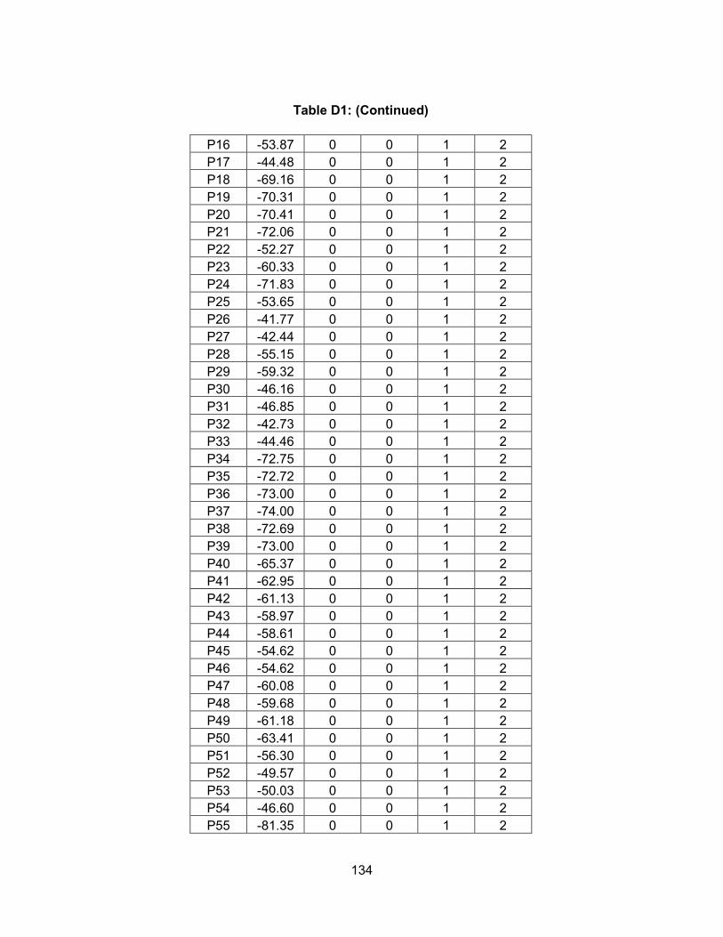
134
Table D1: (Continued)
P16 -53.87 0 0 1 2
P17 -44.48 0 0 1 2
P18 -69.16 0 0 1 2
P19 -70.31 0 0 1 2
P20 -70.41 0 0 1 2
P21 -72.06 0 0 1 2
P22 -52.27 0 0 1 2
P23 -60.33 0 0 1 2
P24 -71.83 0 0 1 2
P25 -53.65 0 0 1 2
P26 -41.77 0 0 1 2
P27 -42.44 0 0 1 2
P28 -55.15 0 0 1 2
P29 -59.32 0 0 1 2
P30 -46.16 0 0 1 2
P31 -46.85 0 0 1 2
P32 -42.73 0 0 1 2
P33 -44.46 0 0 1 2
P34 -72.75 0 0 1 2
P35 -72.72 0 0 1 2
P36 -73.00 0 0 1 2
P37 -74.00 0 0 1 2
P38 -72.69 0 0 1 2
P39 -73.00 0 0 1 2
P40 -65.37 0 0 1 2
P41 -62.95 0 0 1 2
P42 -61.13 0 0 1 2
P43 -58.97 0 0 1 2
P44 -58.61 0 0 1 2
P45 -54.62 0 0 1 2
P46 -54.62 0 0 1 2
P47 -60.08 0 0 1 2
P48 -59.68 0 0 1 2
P49 -61.18 0 0 1 2
P50 -63.41 0 0 1 2
P51 -56.30 0 0 1 2
P52 -49.57 0 0 1 2
P53 -50.03 0 0 1 2
P54 -46.60 0 0 1 2
P55 -81.35 0 0 1 2
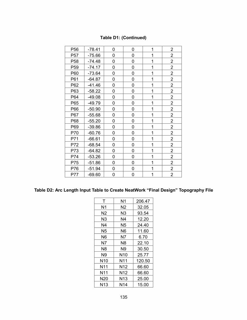
135
Table D1: (Continued)
P56 -78.41 0 0 1 2
P57 -75.66 0 0 1 2
P58 -74.48 0 0 1 2
P59 -74.17 0 0 1 2
P60 -73.64 0 0 1 2
P61 -64.87 0 0 1 2
P62 -41.46 0 0 1 2
P63 -58.22 0 0 1 2
P64 -49.08 0 0 1 2
P65 -49.79 0 0 1 2
P66 -50.90 0 0 1 2
P67 -55.68 0 0 1 2
P68 -55.20 0 0 1 2
P69 -39.86 0 0 1 2
P70 -60.76 0 0 1 2
P71 -66.61 0 0 1 2
P72 -68.54 0 0 1 2
P73 -64.82 0 0 1 2
P74 -53.26 0 0 1 2
P75 -51.86 0 0 1 2
P76 -51.94 0 0 1 2
P77 -69.60 0 0 1 2
Table D2: Arc Length Input Table to Create NeatWork “Final Design” Topography File
T N1 206.47
N1 N2 32.05
N2 N3 93.54
N3 N4 12.20
N4 N5 24.40
N5 N6 11.60
N6 N7 6.70
N7 N8 22.10
N8 N9 30.50
N9 N10 25.77
N10 N11 120.50
N11 N12 66.60
N11 N12 66.60
N20 N13 25.00
N13 N14 15.00

136
Table D2: (Continued)
N14 N15 6.10
N15 N16 38.92
N16 N17 21.49
N17 N17.5 25.50
N17.5 N18 5.00
N18 N19 18.30
N12 N20 22.50
N20 N21 23.00
N21 N22 1.00
N12 N23 32.61
N23 N24 33.85
N24 N25 0.50
N8 N26 45.63
N26 N27 131.90
N27 N28 36.00
N28 N29.0 46.10
N7 N29.1 113.15
N29.1 N30 118.97
N30 N31 57.70
N31 N32 15.00
N32 N33.0 15.00
N33.0 N33.1 18.80
N33.1 N34 35.90
N34 N35 38.75
N30 N36 21.90
N36 N37.0 20.02
N32 N37.5 103.25
N29.0 N38 34.00
N38 N39 25.00
N38 N40 0.50
N40 N41 13.30
N41 N42 17.60
N42 N43 94.20
N43 N44 6.40
N44 N45 14.10
N45 N46 52.55
N46 N47 21.35
N47 N48 29.95
N48 N49 8.53
N48 N50 35.75

137
Table D2: (Continued)
N50 N51 7.10
N51 N52 47.80
N52 N53 24.40
N53 N54 42.70
N46 N47 21.35
N47 N48 29.95
N48 N49 8.53
N48 N50 35.75
N50 N51 7.10
N51 N52 47.80
N52 N53 24.40
N53 N54 42.70
N54 N55 46.79
N55 N56 24.40
N56 N57 36.60
N57 N58 36.60
N58 N59 26.22
N59 N60 24.40
N60 N61 24.40
N61 N62 6.10
N62 N63 6.10
N63 N64 2.70
N63 N65 72.02
N42 N66 26.00
N66 N67 4.20
N67 N68 47.53
N68 N69 67.10
N69 N70 21.74
N69 N71 139.00
N71 N72 21.35
N72 N73 18.30
N73 N74 18.30
N74 N75 6.10
N75 N76 79.85
N72 N77 61.80
N77 N78 42.64
N78 N79 12.00
N79 N80 30.00
N80 N81 23.50
N81 N82 20.60

138
Table D2: (Continued)
N82 N83 3.90
N83 N84 29.69
N77 N85 230.00
N85 N86 68.99
N86 N87 7.00
N87 N88 35.68
N88 N89 20.00
N89 N90 47.97
N90 N91 37.87
N91 N92 6.00
N92 N93 47.48
N93 N94 18.00
N3 P1 19.37
N4 P2 13.07
N5 P3 9.63
N6 P4 145.67
N9 P5 18.30
N10 P6 0.50
N11 P7 25.00
N13 P8 11.80
N14 P9 19.83
N16 P10 17.25
N17 P11 34.30
N18 P12 40.18
N19 P13 12.20
N19 P14 36.60
N21 P15 2.70
N22 P16 26.88
N17.5 P17 80.00
N23 P18 18.30
N24 P19 18.30
N25 P20 14.87
N25 P21 54.90
N26 P22 20.00
N27 P23 20.00
N28 P24 35.00
N33.1 P25 9.80
N36 P26 6.00
N37.0 P27 12.00
N34 P28 6.00

139
Table D2: (Continued)
N35 P29 33.03
N33.0 P30 20.00
N32 P31 20.00
N37.5 P32 6.00
N37.5 P33 35.50
N39 P34 10.00
N39 P35 10.00
N40 P36 20.00
N41 P37 20.00
N43 P38 18.77
N44 P39 0.50
N46 P40 0.50
N49 P41 64.58
N49 P42 4.50
N50 P43 13.00
N52 P44 26.27
N53 P45 35.90
N54 P46 20.20
N55 P47 28.70
N56 P48 6.10
N58 P49 50.84
N60 P50 72.92
N64 P51 4.80
N64 P52 17.31
N65 P53 6.10
N65 P54 23.00
N68 P55 13.55
N70 P56 5.00
N70 P57 40.04
N73 P58 0.50
N74 P59 12.20
N75 P60 12.20
N76 P61 8.00
N77 P62 66.74
N78 P63 6.00
N79 P64 10.43
N80 P65 6.00
N81 P66 1.20
N82 P67 14.60
N83 P68 3.00

140
Table D2: (Continued)
N84 P69 153.75
N85 P70 45.88
N88 P71 64.95
N89 P72 66.76
N90 P73 6.00
N92 P74 36.48
N93 P75 30.00
N94 P76 6.00
N91 P77 150.00
Table D3: NeatWork Simulation Results for “Final Design” Design File
Faucet Idea
No. of Occurrences
Min Flow (L/s)
Average Flow (L/s)
Max Flow (L/s)
Variability (%)
Flow <0.1 L/s (%)
Flow <0.3 L/s (%)
No. of Failures
Global average
0.1899 1.23 0.71 0
P1 35 0.1937 0.1943 0.1954 0.21 0 0 0
P10 46 0.1647 0.2023 0.2803 12.63 0 0 0
P11 31 0.1644 0.1992 0.2705 11.01 0 0 0
P12 49 0.0792 0.1969 0.3451 28.31 4.08 4.08 0
P13 37 0.1397 0.2062 0.3113 19.05 0 2.7 0
P14 39 0.1327 0.2263 0.373 23.26 0 12.82 0
P15 37 0.1616 0.1865 0.2316 9.73 0 0 0
P16 35 0.1489 0.1841 0.2495 11.02 0 0 0
P17 36 0.0232 0.1851 0.3571 38.61 11.11 8.33 0
P18 38 0.1245 0.155 0.1846 10.07 0 0 0
P19 39 0.1545 0.2152 0.2624 12.76 0 0 0
P2 40 0.1959 0.1967 0.1983 0.24 0 0 0
P20 36 0.1554 0.22 0.2925 15.1 0 0 0
P21 45 0.1576 0.2184 0.2964 13.56 0 0 0
P22 36 0.1741 0.1769 0.1798 0.74 0 0 0
P23 41 0.1788 0.1837 0.1898 1.26 0 0 0
P24 39 0.1978 0.2027 0.2094 1.17 0 0 0
P25 43 0.1321 0.1811 0.2526 15.77 0 0 0
P26 39 0.1605 0.1895 0.236 9.83 0 0 0
P27 41 0.1596 0.1887 0.2182 8.71 0 0 0
P28 39 0.1233 0.1772 0.2424 17.92 0 0 0

141
Table D3: (Continued)
P29 38 0.1405 0.178 0.2291 12.78 0 0 0
P3 41 0.1904 0.1915 0.1933 0.29 0 0 0
P30 39 0.129 0.2034 0.314 20.22 0 2.56 0
P31 46 0.1635 0.2266 0.323 17.43 0 6.52 0
P32 38 0.0582 0.1912 0.3404 37.13 10.53 2.63 0
P33 37 0.1123 0.1918 0.3098 27.35 0 5.41 0
P34 45 0.1882 0.1958 0.2066 2.05 0 0 0
P35 44 0.1882 0.1958 0.2046 2.07 0 0 0
P36 35 0.1946 0.2009 0.2101 1.56 0 0 0
P37 33 0.1956 0.2021 0.2096 1.53 0 0 0
P38 41 0.1844 0.1945 0.2028 1.96 0 0 0
P39 39 0.1863 0.1965 0.2068 2.14 0 0 0
P4 41 0.1837 0.1849 0.1863 0.33 0 0 0
P40 39 0.165 0.1768 0.1952 3.2 0 0 0
P41 50 0.1493 0.1648 0.1837 3.7 0 0 0
P42 41 0.149 0.1635 0.1743 3.44 0 0 0
P43 43 0.1435 0.1577 0.1716 3.37 0 0 0
P44 34 0.1994 0.2202 0.2509 4.65 0 0 0
P45 40 0.1703 0.1973 0.2223 5.51 0 0 0
P46 42 0.1584 0.1956 0.2354 8.79 0 0 0
P47 47 0.1743 0.209 0.2472 7.66 0 0 0
P48 44 0.1728 0.2059 0.2442 7.67 0 0 0
P49 41 0.1661 0.2004 0.2436 9.3 0 0 0
P5 38 0.1877 0.1893 0.192 0.48 0 0 0
P50 48 0.1707 0.2003 0.2475 7.91 0 0 0
P51 40 0.1451 0.1774 0.2399 11.32 0 0 0
P52 33 0.1178 0.1826 0.2516 17.54 0 0 0
P53 31 0.1392 0.185 0.2575 19.19 0 0 0
P54 40 0.0465 0.1843 0.3197 41.94 22.5 5 0
P55 45 0.204 0.2113 0.2202 1.71 0 0 0
P56 39 0.1877 0.198 0.209 2.57 0 0 0
P57 42 0.1787 0.1891 0.2015 2.85 0 0 0
P58 41 0.1668 0.18 0.1978 4.08 0 0 0
P59 37 0.1564 0.1739 0.1911 5.96 0 0 0
P6 48 0.1892 0.1922 0.1987 1.11 0 0 0
P60 35 0.1532 0.17 0.188 5.74 0 0 0
P61 40 0.1791 0.2073 0.234 7.29 0 0 0
P62 45 0.1164 0.1852 0.2544 16.87 0 0 0

142
Table D3: (Continued)
P63 38 0.192 0.2139 0.2429 6.19 0 0 0
P64 37 0.1394 0.1706 0.2031 8.71 0 0 0
P65 36 0.1423 0.1675 0.2095 8.85 0 0 0
P66 46 0.1528 0.1795 0.215 8.57 0 0 0
P67 37 0.1734 0.1982 0.2273 6.66 0 0 0
P68 44 0.1758 0.195 0.2324 6.02 0 0 0
P69 53 0.0518 0.1341 0.2085 27.72 22.64 0 0
P7 38 0.1755 0.185 0.2002 3.54 0 0 0
P70 47 0.1706 0.1969 0.2346 7.27 0 0 0
P71 32 0.1682 0.2041 0.2559 10.26 0 0 0
P72 40 0.1738 0.2104 0.2494 8.5 0 0 0
P73 39 0.1608 0.2018 0.2621 11.67 0 0 0
P74 51 0.0804 0.1716 0.2629 21.69 3.92 0 0
P75 41 0.0563 0.1872 0.2849 25.21 7.32 0 0
P76 39 0.0647 0.2022 0.3113 26.13 5.13 5.13 0
P77 39 0.1132 0.1347 0.1636 8.38 0 0 0
P8 44 0.1512 0.1695 0.2108 7.19 0 0 0
P9 38 0.1431 0.1623 0.189 7.72 0 0 0

143
Appendix E: Calculations of Available Head at Each Faucet
Equations used in calculating available head are:
�� = �∗�� (E1)
where:
v = 1.0 x 10⁻⁶ ms/s (Crowe et al., 2010)
= .� ������� ��
�.��� �.�����.� !
" (2)
ℎ$ = %&
�"
�� (1)
'()*+ -�*.+(// = ∑ℎ$ (E2)
12*3+*4+� -�*. = −6 − ℎ$ (E3)
Table E1: Spreadsheet Used to Calculate Available Head at Each Faucet
Start End Length,
L (m)
Pipe Diameter,
d (m)
Average Veloc-
ity, v (m/s)
Reynolds Number,
Re
Friction Factor, f
Head-loss,
hL (m)
Total Head-
loss (m)
Relative Elevation,
E (m)
Calculated Available Head (m)
T N1 14.85 0.082 1.06 86920 0.018 0.19 0.19 -4.0 3.8
N1 N2 17.2 0.082 1.06 86920 0.018 0.22 0.41 -2.6 2.2

144
Table E1: (Continued)
N2 N3 93.54 0.082 1.06 86920 0.018 1.20 1.61 -24.6 23.0
N3 N4 12.2 0.082 1.04 85280 0.018 0.15 1.77 -26.1 24.4
N4 N5 24.4 0.082 1.03 84460 0.019 0.30 2.06 -27.7 25.6
N5 N6 11.6 0.082 1.01 82820 0.019 0.14 2.20 -27.5 25.3
N6 N7 6.7 0.082 0.99 81180 0.019 0.08 2.28 -27.4 25.1
N7 N8 22.1 0.082 0.99 81180 0.019 0.25 2.53 -28.3 25.8
N8 N9 42.7 0.0446 0.85 37910 0.022 0.78 3.31 -32.5 29.2
N9 N10 25.77 0.0446 0.79 35234 0.023 0.41 3.72 -36.1 32.4
N10 N10$ 54 0.0446 0.72 32112 0.023 0.74 4.46
N10$ N11 46.76 0.0304 1.56 47424 0.021 4.01 8.47 -47.1 38.6
N11 N12 48.8 0.0304 1.45 44080 0.021 3.68 12.15 -46.2 34.1
N12 N13 12.2 0.0304 0.74 22496 0.025 0.28 12.43 -46.1 33.7
N13 N14 15 0.0304 0.63 19152 0.026 0.26 12.69 -45.7 33.0
N14 N15 6.1 0.0304 0.49 14896 0.028 0.07 12.76 -45.3 32.6
N15 N16 38.92 0.0304 0.49 14896 0.028 0.44 13.19 -37.1 23.9
N16 N17 21.49 0.0304 0.4 12160 0.029 0.17 13.36 -33.8 20.4
N17 N18 30.5 0.0304 0.3 9120 0.032 0.15 13.51 -27.3 13.7
N18 N19 18.3 0.0182 0.57 10374 0.031 0.51 14.02 -26.1 12.1
N12 N20 37.433 0.0304 0.33 10032 0.031 0.21 12.36 -45.7 33.4
N20 N21 29.958 0.0304 0.33 10032 0.031 0.17 12.53 -36.7 24.2
N21 N22 23.322 0.0304 0.33 10032 0.031 0.13 12.66 -31.9 19.2
N12 N23 32.61 0.0182 1.07 19474 0.026 2.72 14.86 -46.2 31.3
N23 N24 33.85 0.0182 0.8 14560 0.028 1.70 16.56 -46.7 30.1
N8 N25 12.2 0.082 0.74 60680 0.020 0.08 2.61 -27.9 25.3
N25 N26 33.43 0.082 0.74 60680 0.020 0.23 2.84 -27.9 25.1
N26 N27 48.8 0.082 0.72 59040 0.020 0.31 3.15 -33.6 30.4
N27 N28 5 0.082 0.72 59040 0.020 0.03 3.18 -36.9 33.7
N28 N29 42.85 0.0557 1.53 85221 0.018 1.70 4.88 -38.4 33.5

145
Table E1: (Continued)
N29 N30 4.5 0.0557 1.53 85221 0.018 0.18 5.06 -38.9 33.8
N30 N31 7.8 0.0304 1.04 31616 0.023 0.33 5.39 -37.1 31.7
N31 N32 34.08 0.0304 1.04 31616 0.023 1.43 6.81 -49.5 42.7
N32 N33 59.35 0.0304 1.04 31616 0.023 2.49 9.30 -29.3 20.0
N33 N34 6.1 0.0304 1.04 31616 0.023 0.26 9.55 -29.1 19.5
N34 N35 20.7 0.0304 0.94 28576 0.024 0.73 10.28 -25.8 15.5
N35 N36 35.9 0.0304 0.62 18848 0.026 0.61 10.89 -22.6 11.7
N36 N37* 36.25 0.0182 0.54 9828 0.031 0.92 11.81 -30.9 19.1
N36 N38 1.55 0.0304 0.43 13072 0.029 0.01 10.90 -22.7 11.8
N38 N39 10.07 0.0304 0.3 9120 0.032 0.05 10.95 -23.9 12.9
N39 N39$ 73.24 0.0304 0.2 6080 0.036 0.18 11.12
N39$ N40 30 0.0182 0.56 10192 0.031 0.81 11.93 -17.7 5.7
N35 N41 48.8 0.0304 0.31 9424 0.031 0.25 10.53 -23.0 12.4
N41 N41$ 17.2 0.0304 0.21 6384 0.035 0.04 10.57
N41$ N42 15.5 0.0182 0.57 10374 0.031 0.43 11.00 -20.8 9.8
N30 N43 2.3 0.0557 1.22 67954 0.019 0.06 5.12 -39.2 34.1
N43 N44 18.3 0.0557 1.22 67954 0.019 0.48 5.60 -40.4 34.8
N44 N45 16.08 0.0557 1.22 67954 0.019 0.42 6.03 -55.4 49.3
N45 N46 37.2 0.0557 1.22 67954 0.019 0.98 7.01 -48.3 41.3
N46 N47 30.5 0.0446 0.91 40586 0.022 0.63 7.64 -47.6 40.0
N47 N48 40 0.0446 0.91 40586 0.022 0.82 8.46 -48.3 39.9
N48 N49 50 0.0446 0.82 36572 0.022 0.86 9.32 -52.7 43.3
N49 N50 4.2 0.0446 0.82 36572 0.022 0.07 9.39 -54.5 45.1
N50 N51 139 0.0446 0.82 36572 0.022 2.38 11.78 -51.3 39.5
N51 N52 21.35 0.0446 0.82 36572 0.022 0.37 12.14 -51.5 39.3
N52 N53 18.3 0.0182 1.15 20930 0.026 1.73 13.87 -50.1 36.2
N53 N54 18.3 0.0182 0.85 15470 0.028 1.02 14.89 -49.9 35.0
N54 N55 6.1 0.0182 0.55 10010 0.031 0.16 15.05 -49.7 34.6

146
Table E1: (Continued)
N55 N56 79.85 0.0182 0.3 5460 0.037 0.74 15.80 -40.1 24.3
N46 N57 12.2 0.0446 0.98 43708 0.021 0.29 7.30 -48.9 41.6
N57 N58 18.7 0.0446 0.89 39694 0.022 0.37 7.67 -48.6 40.9
N58 N59 49.1 0.0446 0.84 37464 0.022 0.88 8.55 -53.1 44.5
N59 N60 52.55 0.0446 0.84 37464 0.022 0.94 9.49 -41.0 31.5
N60 N61 21.35 0.0446 0.77 34342 0.023 0.33 9.81 -39.0 29.2
N61 N62 29.95 0.0446 0.77 34342 0.023 0.46 10.27 -35.9 25.6
N62 N63 8.53 0.0182 0.29 5278 0.037 0.07 10.35 -36.9 26.6
N62 N64 35.75 0.0446 0.68 30328 0.023 0.44 10.71 -33.7 23.0
N64 N65 7.1 0.0446 0.63 28098 0.024 0.08 10.79 -33.5 22.7
N65 N66 47.8 0.0446 0.63 28098 0.024 0.51 11.31 -33.2 21.9
N66 N67 24.4 0.0446 0.58 25868 0.024 0.23 11.53 -31.7 20.2
N67 N67$ 28.79 0.0446 0.53 23638 0.025 0.23 11.76
N67$ N68 13.91 0.0304 1.13 34352 0.023 0.67 12.44 -30.5 18.1
N68 N69 46.79 0.0304 1.03 31312 0.023 1.93 14.36 -33.6 19.3
N69 N70 24.4 0.0304 0.92 27968 0.024 0.82 15.19 -34.9 19.7
N70 N71 36.6 0.0304 0.81 24624 0.025 0.99 16.17 -36.6 20.5
N71 N72 36.6 0.0304 0.81 24624 0.025 0.99 17.16 -35.4 18.2
N72 N73 26.22 0.0304 0.57 17328 0.027 0.38 17.54 -32.5 14.9
N73 N74 24.4 0.0304 0.48 14592 0.028 0.26 17.81 -31.2 13.4
N74 N75 24.4 0.0304 0.39 11856 0.030 0.18 17.99 -29.4 11.4
N75 N76 6.1 0.0304 0.39 11856 0.030 0.05 18.04 -29.6 11.5
N76 N77 6.1 0.0304 0.39 11856 0.030 0.05 18.08 -31.0 12.9
N77 N78 2.7 0.0182 0.57 10374 0.031 0.08 18.16 -31.1 12.9
N77 N79 72.02 0.0304 0.18 5472 0.037 0.14 18.23 -25.9 7.7
N52 N80 61.8 0.0446 0.62 27652 0.024 0.65 12.79 -47.2 34.4
N80 N81 42.64 0.0446 0.62 27652 0.024 0.45 18.67 -35.0 16.3
N81 N82 12 0.0446 0.59 26314 0.024 0.12 12.91 -33.2 20.3

147
Table E1: (Continued)
N82 N83 30 0.0446 0.53 23638 0.025 0.24 18.91 -28.1 9.2
N83 N84 23.5 0.0446 0.48 21408 0.025 0.16 13.06 -25.5 12.4
N84 N85 20.6 0.0446 0.44 19624 0.026 0.12 19.03 -26.6 7.6
N85 N86 3.9 0.0446 0.38 16948 0.027 0.02 13.08 -26.9 13.8
N86 N87 29.69 0.0446 0.34 15164 0.028 0.11 19.14 -30.9 11.7
N87 N88 6 0.0446 0.29 12934 0.029 0.02 13.10 -31.9 18.8
N88 N89 68.99 0.0304 0.58 17632 0.027 1.04 20.18 -43.6 23.4
N89 N90 7 0.0304 0.47 14288 0.028 0.07 13.17 -41.9 28.7
N90 N90$ 22.68 0.0304 0.47 14288 0.028 0.24 20.41
N90$ N91 13 0.0304 1.3 39520 0.022 0.81 13.98 -45.5 31.6
N91 N92 20 0.0182 1.02 18564 0.026 1.53 21.95 -48.7 26.8
N92 N93 47.97 0.0182 0.67 12194 0.029 1.77 15.75 -39.9 24.2
N93 N94 37.87 0.0182 0.42 7644 0.033 0.62 22.57 -36.0 13.4
N94 N95 6 0.0182 0.42 7644 0.033 0.10 15.85 -35.3 19.5
N95 N96 47.48 0.0182 0.26 4732 0.038 0.35 22.92 -27.4 4.4
N96 N97 18 0.0182 0.26 4732 0.038 0.13 15.98 -27.4 11.5
N11 N1* 2.14 0.0182 0.3 5460 0.037 0.02 8.49 -45.8 37.3
N18 N2* 6.1 0.0182 0.27 4914 0.038 0.05 13.56 -25.9 12.3
N2* N3* 27.98 0.0182 0.27 4914 0.038 0.22 8.71 -20.3 11.6
N39 N4* 22.45 0.0182 0.29 5278 0.037 0.20 11.14 -22.5 11.4
N88 N6* 65.5 0.0304 0.05 1520 0.056 0.02 8.72 -41.7 33.0
N91 N7* 10.95 0.0182 0.28 5096 0.038 0.09 14.07 -40.1 26.0
N7* N8* 24 0.0182 0.28 5096 0.038 0.20 22.15 -38.2 16.1
N92 N9* 8 0.0182 0.36 6552 0.035 0.10 15.85 -45.0 29.2
N57 N5* 6.1 0.0182 0.69 12558 0.029 0.24 7.54 -48.3 40.8
N3 P1 19.37 0.0182 0.83 15106 0.028 1.04 2.65 -27.8 25.1
N4 PN1 13.07 0.0182 0.86 15652 0.027 0.74 2.51 -29.8 27.3
N5 P2 9.63 0.0182 0.85 15470 0.028 0.54 2.60 -29.3 26.7

148
Table E1: (Continued)
N6 P3 145.67 0.0182 0.8 14560 0.028 7.31 9.51 -32.9 23.4
N9 P4 18.3 0.0182 0.87 15834 0.027 1.06 4.37 -32.4 28.1
N10 P5 0.5 0.0182 0.93 16926 0.027 0.03 3.75 -36.1 32.4
N1* P6 8.64 0.0182 0.66 12012 0.029 0.31 8.80 -46.4 37.6
N13 P7 11.8 0.0182 0.91 16562 0.027 0.74 13.17 -46.1 32.9
N14 P8 19.83 0.0182 0.87 15834 0.027 1.15 13.84 -43.9 30.1
N16 P9 17.25 0.0182 0.72 13104 0.029 0.72 13.91 -34.6 20.7
N17 P10 34.3 0.0182 0.71 12922 0.029 1.40 14.76 -35.5 20.7
N19 P11 12.2 0.0182 0.76 13832 0.028 0.56 14.58 -26.0 11.5
N19 P12 36.6 0.0182 0.71 12922 0.029 1.49 15.51 -23.2 7.7
N3* P13 6.1 0.0182 0.77 14014 0.028 0.29 8.99 -20.9 11.9
N22 P14 55 0.0182 0.68 12376 0.029 2.08 14.74 -20.1 5.4
N22 P15 2.7 0.0182 0.9 16380 0.027 0.17 12.83 -31.1 18.3
N22 P16 26.88 0.0182 0.82 14924 0.028 1.41 14.07 -29.5 15.4
N23 P17 18.3 0.0182 0.82 14924 0.028 0.96 15.82 -44.8 29.0
N24 P18 18.3 0.0182 0.77 14014 0.028 0.86 17.42 -45.9 28.5
N24 P19 14.87 0.0182 0.79 14378 0.028 0.73 17.29 -46.0 28.7
N24 PN2 54.9 0.0182 0.76 13832 0.028 2.52 19.09 -47.7 28.6
N26 P20 0.8 0.0182 0.82 14924 0.028 0.04 2.88 -27.9 25.0
N28 PN3 14.1 0.0182 0.93 16926 0.027 0.92 4.10 -35.9 31.8
N37* P21 2.5 0.0182 0.67 12194 0.029 0.09 11.90 -31.4 19.5
N37* P22 35.53 0.0182 0.72 13104 0.029 1.49 13.29 -35.5 22.2
N34 P23 30.5 0.0182 0.69 12558 0.029 1.18 10.74 -29.9 19.1
N38 P24 4.78 0.0182 0.87 15834 0.027 0.28 11.18 -22.4 11.2
N4* P25 31.75 0.0182 0.77 14014 0.028 1.49 12.64 -23.1 10.4
N40 P26 0.5 0.0182 0.67 12194 0.029 0.02 11.95 -17.3 5.4
N40 P27 35.5 0.0182 0.71 12922 0.029 1.45 13.38 -19.1 5.7
N41 PN4 8.54 0.0182 0.75 13650 0.028 0.38 10.91 -23.8 12.9

149
Table E1: (Continued)
N42 P28 42.7 0.0182 0.75 13650 0.028 1.92 12.92 -18.0 5.1
N42 P29 20.85 0.0182 0.81 14742 0.028 1.07 12.07 -19.8 7.7
N57 P30 24.87 0.0182 0.69 12558 0.029 0.97 8.26 -48.3 40.0
N58 P31 0.5 0.0182 0.69 12558 0.029 0.02 7.69 -48.6 40.9
N60 P32 0.5 0.0182 0.91 16562 0.027 0.03 9.52 -41.0 31.5
N62 P33 64.58 0.0182 0.8 14560 0.028 3.24 13.52 -38.6 25.1
N63 P34 4.5 0.0182 0.82 14924 0.028 0.24 10.59 -36.7 26.2
N64 P35 13 0.0182 0.78 14196 0.028 0.62 11.34 -34.6 23.2
N66 P36 26.27 0.0182 0.75 13650 0.028 1.18 12.49 -34.2 21.7
N67 P37 35.9 0.0182 0.66 12012 0.029 1.29 12.82 -30.2 17.4
N68 PN5 20.2 0.0182 0.65 11830 0.030 0.71 13.14 -30.2 17.1
N69 P38 28.7 0.0182 0.71 12922 0.029 1.17 15.53 -35.7 20.2
N70 P39 6.1 0.0182 0.7 12740 0.029 0.24 15.43 -35.3 19.9
N72 P40 50.84 0.0182 0.66 12012 0.029 1.83 18.99 -36.8 17.8
N73 P41 11 0.0182 0.79 14378 0.028 0.54 18.08 -33.7 15.6
N74 P42 72.92 0.0182 0.67 12194 0.029 2.69 20.50 -39.0 18.5
N78 P43 4.8 0.0182 0.74 13468 0.029 0.21 18.37 -31.9 13.5
N78 P44 17.31 0.0182 0.64 11648 0.030 0.59 18.75 -25.2 6.4
N79 N79$ 17 0.0304 0.17 5168 0.037 0.03 18.26
N79$ P45 6 0.0182 0.23 4186 0.040 0.04 18.29 -22.2 3.9
N79 PN6 6.1 0.0182 0.7 12740 0.029 0.24 18.47 -25.6 7.2
N72 P46 14.2 0.0182 0.86 15652 0.027 0.81 17.97 -47.4 29.5
N48 P47 6.9 0.0182 0.68 12376 0.029 0.26 8.73 -48.3 39.6
N48 P48 7.53 0.0182 0.68 12376 0.029 0.29 8.75 -48.4 39.6
N53 PN7 0.5 0.0182 0.64 11648 0.030 0.02 13.89 -50.1 36.2
N54 PN8 12.2 0.0182 0.61 11102 0.030 0.38 15.28 -49.8 34.5
N55 P49 12.2 0.0182 0.6 10920 0.030 0.37 15.43 -49.3 33.8
N56 P50 8 0.0182 0.7 12740 0.029 0.32 16.12 -40.5 24.4

150
Table E1: (Continued)
N81 P51 66.74 0.0182 0.5 9100 0.032 1.49 20.16 -17.1 -3.1
N82 PN9 6 0.0182 0.64 11648 0.030 0.20 13.11 -33.8 20.7
N83 PN10 10.43 0.0182 0.69 12558 0.029 0.41 19.32 -24.7 5.4
N84 P52 6 0.0182 0.71 12922 0.029 0.24 13.31 -25.4 12.1
N85 P53 1.2 0.0182 0.76 13832 0.028 0.06 19.09 -26.5 7.4
N86 P54 14.6 0.0182 0.65 11830 0.030 0.51 13.59 -31.3 17.7
N87 P55 3 0.0182 0.65 11830 0.030 0.11 19.25 -30.8 11.6
N6* N6*$ 147.75 0.0304 0.1 3040 0.044 0.11 8.83
N6*$ P56 6 0.0182 0.13 2366 0.048 0.01 8.85 -15.5 6.6
N89 P57 45.88 0.0182 0.69 12558 0.029 1.78 21.96 -36.4 14.4
N8* P58 30 0.0182 0.73 13286 0.029 1.28 23.43 -42.2 18.8
N9* P59 58.76 0.0182 0.73 13286 0.029 2.52 18.37 -44.2 25.8
N93 PN11 6 0.0182 0.66 12012 0.029 0.22 15.96 -40.4 24.5
N95 PN12 36.48 0.0182 0.43 7826 0.033 0.63 16.47 -28.9 12.4
N97 P60 6 0.0182 0.37 6734 0.035 0.08 16.06 -27.5 11.4
N97 PN13 30 0.0182 0.38 6916 0.034 0.42 16.39 -27.6 11.2

151
Appendix F: Determining an Appropriate Number of Future Connections
The current standard for assuring water sources will have enough water in the future is
to calculate the water needs of a future population calculated by a growth rate equation over the
life of the aqueduct, typically 20 years. Assuming the average number of people per house
remains constant as houses are added to the system, the same growth rate equation, Equation
9, can be used to calculate the future number of connections needed as follows:
78 = 79 ∗ �1 + <×8> (F1)
In Equation F1:
CN = the future number of connections
C0 = the current number of connections
R = rate of growth
N = number of years
The confirmed Santa Cruz aqueduct has 60 connections. Using Equation F1 and the
Panamanian growth rate of 1.32% (CIA World Factbook, 2016), the projected number of
connections for the Santa Cruz aqueduct in 20 years is calculated to be 75 connections or 15
new connections.
The author ran an analysis on an aqueduct that would have 13 new connections which is
2 less than the projected number of connections based on the modeled population growth.
While adding two additional houses will continue to decrease the quality of service, it will not be
significant enough to hurt the sustainability of the aqueduct. Therefore, using 13 houses for the

152
analysis is appropriate for this analysis and represents a reasonable number of houses that
could be added to the aqueduct in the future.
The author demonstrated that the Santa Cruz aqueduct still works at a reliable level of
service when additional connections are added in conjunction with the predicted number of
future connections based on the population growth rate. The author assumes that this will hold
true for other aqueducts during their life as connections are added, but there is no evidence to
support this claim. As stated earlier, for best results the designer should include all known
potential connections in the design to minimize reductions in service quality throughout the life
of the aqueduct.

153
Appendix G: Copyright Permissions
The following shows that no formal permission is needed for the reproduction of Figure
2.