investigation and validation of stability for the
TRANSCRIPT

©
foto
pro
-
Institute of Electrical Power Systems
Investigation and Validation
of Stability for the
Photovoltaic Integration into
a Medium Voltage Grid
Based on PHIL Testing
A Master thesis by
Carina Lehmal, BSc.
Supervisor
Ziqian Zhang, Dipl.-Ing. Dr.techn.
Reviewer
Ziqian Zhang, Dipl.-Ing. Dr.techn.
Lothar Fickert, Em.Univ.-Prof. Dipl.-Ing. Dr.techn.
September 2021

Investigation and Validation of Stability for the Photovoltaic Integration into a Medium Voltage Grid Based on PHIL Testing
II
Graz University of Technology
Institute of Electric Power Systems
Inffeldgasse 18/I
8010 Graz
Austria
Head of Institute
Robert Schürhuber
Supervisor
Ziqian Zhang, Dipl.-Ing. Dr.techn.
Reviewer
Ziqian Zhang, Dipl.-Ing. Dr.techn.
Lothar Fickert, Em.Univ.-Prof. Dipl.-Ing. Dr.techn.
A Master thesis by
Carina Lehmal, BSc.
09 2021

Investigation and Validation of Stability for the Photovoltaic Integration into a Medium Voltage Grid Based on PHIL Testing
III
Statutory Declaration
I declare that I have authored this thesis independently, that I have not used other than the declared
sources / resources, and that I have explicitly marked all material, which has been quoted either literally
or by content from the used sources.
Graz, 05.09.2021 Carina Lehmal
Eidesstattliche Erklärung
Ich erkläre an Eides statt, dass ich die vorliegende Arbeit selbstständig verfasst, andere als die
angegebenen Quellen/Hilfsmittel nicht benutzt, und die den benutzten Quellen wörtlich und inhaltlich
entnommenen Stellen als solche kenntlich gemacht habe.
Graz, am 05.09.2021 Carina Lehmal

Investigation and Validation of Stability for the Photovoltaic Integration into a Medium Voltage Grid Based on PHIL Testing
IV
Acknowledgements
First of all, I would like to express my sincerest gratitude to my supervisor, Dr. Ziqian Zhang, for his
guidance starting from the beginning of the master thesis. His motivation to familiarize me with a topic
that was foreign to me at the start and to patiently explain every concept and question in detail, building
on the background I had already acquired during my bachelor and master's studies, helped me to
expand my knowledge and to set up this master's thesis in a technically correct manner. During the
realisation of the master thesis, he not only clarified the theoretical side and guided me concretely to the
correct result in the mathematical models, but also actively supported me in the PHILlab during the
execution of the experimental experiments. Due to our successful teamwork, the discussed topics of
this master thesis as well as the experiments could be carried out thoroughly.
At this place, I would like to thank my Master's examiners Professor Dr. Schürhuber and Professor Dr.
Krischan for their help in courses and their open ear whenever I had any questions. Their courses in my
studies laid the foundations on which I was able to successfully build for this master's thesis.
Also, I am very grateful to Professor Dr. Lothar Fickert, who integrated me into his project in cooperation
with the company Borealis Polyolefine GmbH and thus gave me the chance to be able to set up this
master's thesis in the first place. He further enhanced my knowledge through in-depth discussions and
passed on useful tips for considering the reasonableness of calculation, simulation and measurement
results.
Next, I would like to thank the company Borealis Polyolefine GmbH for the opportunity to carry out this
master thesis. I would especially like to mention Mr. Haslinger, who was always there for all performed
measurements on company perimeters and who took perfect care of me when I had any questions. His
commitment made it possible for me to get to know the company Borealis Polyolefine GmbH, attend
meetings and gain an insight into working life.
Furthermore, I would like to thank the whole team of IEAN, especially DI Manuel Galler and DI Philipp
Hackl, for the pleasant working environment, the meaningful technical discussions and help with all the
small or big questions during measurements in the PHILlab.
Last, but most importantly, I would like to express my deepest gratitude to my mom and my friends. My
mom’s faith in me and unconditional love and support as well as all the long evenings with my friends
that always put a smile on my face when I was not in such a positive mood.

Investigation and Validation of Stability for the Photovoltaic Integration into a Medium Voltage Grid Based on PHIL Testing
V
Abstract
The integration of renewable energies into the voltage grid is becoming more and more important in
order to meet the increasing requirements of a clean, safe and sustainable power supply. In this context,
three-phase inverters play a very important role, as they are used to convert energy between different
voltage forms and voltage levels and are thus the most important component when connecting
photovoltaic energies and wind energies to the grid. However, due to their power electronic components,
they suffer from instabilities themselves as well as from instabilities caused by dynamic interactions
between inverter and voltage grid. Therefore, it is necessary to perform a stability analysis depending
on the existing grid impedance before connecting an inverter to the grid.
In the present master thesis, the stability analysis of an 8 MW photovoltaic system into an existing grid
at 6 kV medium voltage level is carried out. A model of the overall system is designed based on
theoretical calculations and validated with on-site measurements. Building on this, an analysis of the
static as well as dynamic stability is executed during subsequent measurements of the inverters in the
test laboratory in order to be able to make a well-founded final statement. The inverter measurements
are performed using the "power-hardware-in-the-loop" test method, which gives a very good overview
of the behaviour of the whole system, while only the inverter is present as real equipment.
Kurzfassung
Die Integration von regenerativen Energien in das Spannungsnetz wird immer wichtiger, um den
steigenden Anforderungen einer sauberen, sicheren und nachhaltigen Energieversorgung gerecht zu
werden. Dabei spielen dreiphasige Wechselrichter eine sehr große Rolle, da sie verwendet werden um
Energie zwischen unterschiedlichen Spannungsformen und Spannungsebenen umzuwandeln und
damit der wichtigste Bestandteil beim Anschluss von Photovoltaik- und Windenergien ans Netz sind.
Allerdings leiden sie durch ihre leistungselektronischen Komponenten selbst an Instabilitäten als auch
an Instabilitäten durch dynamische Interaktionen zwischen Wechselrichter und Spannungsnetz.
Deswegen ist es notwendig eine Stabilitätsbetrachtung vor Installation eines Wechselrichters in
Abhängigkeit von der vorhandenen Netzimpedanz durchzuführen.
In der vorliegenden Masterarbeit wird die Stabilitätsbetrachtung einer 8-MW-Photovoltaikanlage in ein
bestehendes Netz auf 6-kV-Mittelspannungsebene durchgeführt. Dabei wird anhand von theoretischen
Berechnungen und Validierung dieser mit Messungen vor Ort ein Modell des Gesamtsystems
entworfen. Darauf aufbauend kann bei nachfolgenden Messungen der Wechselrichter im Testlabor eine
Analyse der statischen als auch dynamischen Stabilität erstellt werden, um so eine fundierte
Endaussage treffen zu können. Die Messungen der Wechselrichter werden mittels der „Power-
Hardware-in-the-Loop“-Testmethode durchgeführt, welche einen sehr guten Überblick des Verhaltens
des Gesamtsystems gibt, während nur der Wechselrichter als reales Betriebsmittel vorhanden ist.

Investigation and Validation of Stability for the Photovoltaic Integration into a Medium Voltage Grid Based on PHIL Testing
VI
List of Symbols and Abbreviations
A Cable cross-section
AA1-AA4 States of extruder motor and photovoltaic system
Cpos Capacitance of the positive sequence
Czero Capacitance of the zero sequence
cosφ Power factor
DPD Distributed Power System
f Frequency
fs Switching frequency
GNC Generalized Nyquist criterion
IEC 61000-2-4 IEC norm
lcable Length of cable
Lpos Inductance of the positive sequence
Lzero Inductance of the zero sequence
Iν Harmonic current
IA System current
iref Reference current
iS System current
IGBT Insulated-Gate Bipolar Transistor
Ki Integral part of PI controller
Kp Proportional part of PI controller
MV23 A feeder at the main busbar of the industry grid
MV24 A feeder at the main busbar of the industry grid
P Active power of transformer
PHIL-test Power-hardware-in-the-loop test
PI controller Controller with proportional and integral part
PLL Phase Locked Loop
PWM Pulse Width Modulation

Investigation and Validation of Stability for the Photovoltaic Integration into a Medium Voltage Grid Based on PHIL Testing
VII
PV Photovoltaic (DC part of PV system)
PV system Photovoltaic plus inverter
R Resistance of motor
Rpos Resistance of the positive sequence
RT Transformer resistance
Rzero Resistance of the zero sequence
SSM Small signal modelling
SkV Short-circuit power at the connection point
SA Short-circuit power at installation of user
SPV Power of photovoltaic installation
t Time, transformation ratio
THD Total harmonic distortion ratio
TOR-D2 Technical and organisational rules for operators and users of grids - Part D2
ΔU Voltage increase
UDC DC voltage, DC link voltage
uK Transformer short circuit ratio
UOS Transformer voltage at high-voltage level
UUS Transformer voltage at low-voltage level
XT Transformer reactance
YW Inverter admittance
Zg Grid impedance
ZT Transformer impedance
ZW Inverter impedance
Values with -0 Value at 50 Hz operating state
Values with -c Controller variables
Values with -s System variables
Gxx Transfer functions

Investigation and Validation of Stability for the Photovoltaic Integration into a Medium Voltage Grid Based on PHIL Testing
VIII
Table of Contents
1 Introduction ...................................................................................... 1
1.1 Motivation .............................................................................................................................1
1.2 Current status of research ....................................................................................................1
1.2.1 Steady-state validation ........................................................................................................ 1
1.2.2 Stability validation ................................................................................................................ 2
1.2.3 Transient-state validation .................................................................................................... 3
1.3 Aim and task description of this master thesis .....................................................................6
2 Steady-state validation .................................................................... 7
2.1 Design of the industry grid model .........................................................................................7
2.1.1 Calculation of equipment ..................................................................................................... 9
2.1.1.1 Modelling of the main busbar feeder ........................................................................... 9
2.1.1.2 Modelling of the Extrudermotor ................................................................................... 9
2.1.1.3 Modelling of cables .................................................................................................... 10
2.1.1.4 Modelling of transformers .......................................................................................... 10
2.1.1.5 Modelling of other loads ............................................................................................ 12
2.1.1.6 Modelling of photovoltaic and inverter ....................................................................... 12
2.2 Harmonic analysis ............................................................................................................. 13
2.2.1 General .............................................................................................................................. 13
2.2.1.1 Grid codes ................................................................................................................. 13
2.2.2 Basic information on the assessment of the photovoltaic system and the 5.3 MW extruder
.......................................................................................................................................... 14
2.2.3 Rough analysis regarding the necessity of a harmonic analysis ....................................... 14
2.2.4 Analysis of the individual emitted harmonic currents ........................................................ 15
2.2.4.1 Emission limit values for individual harmonic currents according to TOR ................. 16
2.2.4.2 Emission limit values for the total of all harmonic currents THDi according to TOR . 16
2.2.4.3 Calculation ................................................................................................................. 17
2.2.4.4 Results and conclusion .............................................................................................. 18
2.3 Feed-In or withdrawal of power ......................................................................................... 19
2.3.1 Description of the calculation ............................................................................................. 19
2.3.2 Grid parameters ................................................................................................................. 21

Investigation and Validation of Stability for the Photovoltaic Integration into a Medium Voltage Grid Based on PHIL Testing
IX
2.3.3 Calculation ......................................................................................................................... 22
2.3.4 Assessment ....................................................................................................................... 22
2.4 Conclusion of steady-state validation ................................................................................ 23
3 Transient-state validation ............................................................. 24
3.1 Impedance-based approach .............................................................................................. 24
3.1.1 Impedance-based equivalent circuit .................................................................................. 24
3.1.2 Impedance-based stability criterion ................................................................................... 25
3.1.3 Nyquist criterion ................................................................................................................. 25
3.2 Modelling of the grid-inverter system ................................................................................. 27
3.2.1 Modelling in dq-rotating coordinate system (dq system) ................................................... 28
3.2.2 Hardware modelling ........................................................................................................... 30
3.2.3 Small signal modelling of phase locked loop ..................................................................... 31
3.2.4 Current control loop transfer function ................................................................................ 37
3.2.5 Modelling of delay unit ....................................................................................................... 37
3.2.6 Decoupling transfer functions ............................................................................................ 38
3.3 Transfer function of inverter ............................................................................................... 38
3.4 Investigation of modelling results ...................................................................................... 40
3.4.1 Comparison between model with and without PLL ........................................................... 40
3.4.2 Model with PLL with different Padè orders ........................................................................ 42
3.4.3 Comparison between analytical models and photovoltaic model ...................................... 43
3.5 Validation of stability theory ............................................................................................... 44
3.6 Countermeasures for an unstable inverter behaviour ....................................................... 47
4 Field measurement and evaluation .............................................. 49
4.1 Measuring set-up ............................................................................................................... 49
4.1.1 First measurement ............................................................................................................. 50
4.1.1.1 Transformer feeder “MV23” ....................................................................................... 50
4.1.1.2 Motor feeder “MV24”.................................................................................................. 52
4.1.2 Second measurement........................................................................................................ 53
4.2 Comparison and results ..................................................................................................... 54
4.2.1 Comparison between measurement and simulation ......................................................... 54
4.2.1.1 Transformer feeder “MV23” ....................................................................................... 54

Investigation and Validation of Stability for the Photovoltaic Integration into a Medium Voltage Grid Based on PHIL Testing
X
4.2.1.2 Motor feeder “MV24”.................................................................................................. 55
4.3 Photovoltaic system simulation based on field test result ................................................. 56
4.3.1 Transformer feeder “MV23” with photovoltaic system ....................................................... 56
4.3.2 Motor feeder “MV24” with photovoltaic system ................................................................. 57
4.4 Conclusion ......................................................................................................................... 58
4.4.1 Comparison of measurement and simulation .................................................................... 58
4.4.2 Interpretation ...................................................................................................................... 58
5 Laboratory test............................................................................... 59
5.1 Frequency Sweep .............................................................................................................. 59
5.1.1 Method description ............................................................................................................ 59
5.1.1.1 Frequency sweep ...................................................................................................... 61
5.1.1.2 Measurement evaluation in dq-domain ..................................................................... 62
5.1.2 Results of frequency sweeps ............................................................................................. 63
5.1.2.1 Frequency sweeps of real world inverters ................................................................. 63
5.1.2.2 Frequency sweep of grid model ................................................................................ 64
5.1.2.3 Frequency sweep results ........................................................................................... 65
5.2 PHIL – test ......................................................................................................................... 70
5.2.1 Method description ............................................................................................................ 71
5.2.2 Laboratory setup ................................................................................................................ 72
5.2.3 PHIL – test results ............................................................................................................. 73
5.2.3.1 Integrity of PHIL-test .................................................................................................. 73
5.2.3.2 Results of PHIL-test ................................................................................................... 73
6 Summary and findings .................................................................. 75
6.1 Summary ........................................................................................................................... 75
6.2 Outlook .............................................................................................................................. 77
7 Bibliography ................................................................................... 78
8 List of figures ................................................................................. 80
9 List of tables .................................................................................. 81

Introduction
1
1 Introduction
1.1 Motivation
In order for the present power grid to continue to comply with environmental concerns and regulatory
requirements in the future, technology trends and energy storage besides further automation and
communication must be implemented while still meeting the demand of multiplying consumers [1]. With
regard to the required turnaround of a carbon-based conventional power grid towards a sustainable and
low-emission one, renewable energies and their integration, as well as associated problems, must be
taken into account. The focus in this process is on decarbonisation, decentralisation and digitalisation
[1], [2], driven by the employment of electronic power converters [2]. While this transformation promotes
modern power grids with high flexibility, sustainability and improved efficiency, it constitutes new
challenges based on the power electronics and power converters [3], [2].
Considering the wide timescale control dynamics of power converters, the utilised control algorithm of
the converters influences the stability properties of the converter, which in turn determine the stability of
the entire system. In some cases, the cross coupling between the electromechanical dynamics and
electromagnetic over voltages result in undesired oscillation like harmonics, inter-harmonics and
resonances over a wide frequency range [2]. These in turn can cause disruptions in the power supply
as well as premature aging and excessive stress of equipment and insulation even though the used
technologies have been approved and certified for grid compatibility [3]. For this reason, first the causes
must be identified and second the test and validation methodology revised [3], [4].
Literature sources describing these stability problems exist in every sector that uses energy as a
propulsion option. In [5] the problem of harmonics is addressed from wind turbines side, in [6] and [7]
for high-speed electric trains, and in [8], [9] and [10] for photovoltaics.
1.2 Current status of research
1.2.1 Steady-state validation
The steady-state discusses the first source of instability in a grid. This type of instability has existed
since the beginning of the nationwide grid expansion and the ever-increasing interconnection of smaller
sub-grids into a large interconnected grid, for example the ENTSOE grid in Europe [11].
Are AC generators operated parallel, oscillations occur in grid systems due to the power to phase-angle
curve gradient interacting with the rotary inertia of the electric generator. Slight differences in the design
of the loading and generators excite these oscillations continually. For this reason, damper windings
have been installed in generators and the problem seemed to disappear.

Introduction
2
Shortly after, the interconnection of power systems increased and the damper windings reached their
limits. Both interconnected systems noticed the high external impedance of the other system. With that,
the generator voltage becomes a function of angular swings, the voltage regulator steps in and as a
result, negative damping becomes a negative side effect [11].
Nowadays coupled with cables, overhead lines and automatic control of power grids, oscillations in
power grids have many sources specifying the natural resonance frequency completely by the network
impedance itself.
Focussing now on the newer additions to the power grid with a power electronic interface like inverters,
the switches inside the inverter operate with their own switching frequency. Now by the time a connection
between inverter and grid is conducted, these two frequencies influence each other. Here an instability
occurs as soon as the switching frequency is close to the resonance frequency of the grid. The occurring
harmonics can be found in the voltage as well as in the current. Harmonics in voltage originate from
parallel resonances and harmonics in current stem from serial resonances.
Briefly summarised, these oscillations cannot be eliminated, but their frequency and magnitude
modified. Automatic controls of regulators is a big source for negative damping and the interconnection
between power grids multiply oscillations affecting each equipment. Harmonics mostly cause additional
heating of equipment and reduce the lifespan, performance and stability of the equipment [11].
1.2.2 Stability validation
Power system stability exists when the power system has the ability first to find a stable operation point
and then to achieve it again in case of a physical disturbance. Throughout this process, the integrity of
the complete system must be retained, meaning that the no part of the power system can fail its
operation, except for the faulted elements or intentionally tripped ones to guarantee the continuity of the
rest of the power system [11].
Since the power system represented by mathematical equations consists of a high-order nonlinear
multivariable system, its dynamic performance depends of the constantly changing environment
including the responses to loads, generator outputs, changes in topology and key operating parameters.
The stability performance of a power system depends strongly on the type of disturbance. This
disturbance can be both small and large, influencing the response of the power system and in turn
affecting the grid equipment [11].
Normally, there are three types of system stability problems [12]:
Steady-state stability: It exists an equilibrium point of the system, which the system can
maintain.
Small-signal stability: The system has the ability to return to the original operating point after a
minor disturbance. This small perturbation is sufficiently small, that the system equations can
be linearized.

Introduction
3
Large-signal stability: The system has the ability to switch from the original steady operating
point to a new steady operating point after a large disturbance. Here most analysis takes place
with Lyapunov stability.
Due to this, instability of the power system can have different forms, which gives importance to the
analysis of the stability problems. Generally, the classification of power system stability is divided into
three sub-areas [11]:
Rotor angle stability
Frequency stability
Voltage stability
Rotor angle stability deals with the ability of synchronous machines to find an equilibrium between
electromagnetic torque and mechanical torque under normal operating conditions as well as after a
disturbance [11].
Frequency stability is concerned with maintaining a steady frequency, within the nominal range, after a
large disturbance. The aim here is to restore the balance between generation and load with a minimum
loss of load [11].
Voltage stability focuses on maintaining steady voltages on all busbars of the system under normal
operating conditions as well as after disturbances. If the system loses its voltage stability, there can be
a loss of load, loss of grid integrity and, consequently, a loss of synchronism of the rotor angles, which
will cause synchronous machines to fail [11].
Besides the steady-state stability, for rotor angel stability and frequency stability, it makes sense to
distinguish between a small and a large disturbance, as these have a different effect on the behaviour
of the system and on the tools for mathematical description and design of simulation [11], [12].
1.2.3 Transient-state validation
With the transformation of the traditional centralised power system to a decentralised power system with
many individual loads and generation, distributed power system (DPS) technology is becoming
increasingly important. Through DPS, converters can be configured to behave in a certain way and can
be controlled.
Since the control parameters are one of the most sensitive components for a stability analysis in this
transient case, an inappropriate model does not equal reality values and forms an incorrect study. In
general, inverters have a very high bandwidth to control them, which leads to a dynamic interaction
between the inverter and the passive components of the system over a wide frequency range. When
actuating the IGBTs, a PWM with high frequency is used and there is a dead-time in which the
semiconductors are switched off between the duty cycles to avoid short circuits. These two
circumstances add harmonics over a wide spectrum in addition to the fundamental frequency.

Introduction
4
To filter out switching harmonics as well as possible, passive filters such as high-pass or low-pass filters
made of RLC elements are used at the input of the inverter. These passive filters interact with the
passive components of the overall system when the inverter is connected and thus lead to further
harmonics [11].
However, with the addition of a complete inverter-grid model this results in complex systems with
dynamic system interactions that lead to different stability problems [13].
In order to be able to analyse such systems, several analysis approaches exist, each having their own
advantages and disadvantages.
Amongst several approaches the state-space-based approach, the transfer-function-based approach or
impedance-based approach receive most of the attention of scientific studies in regard to feasibility in
praxis.
1.) The state-space-based approach [12], [14], [15], [16], [17]:
This approach is already well known in the analysis of traditional power systems, therefore very
well researched, and deployed in commercial software. In the state-space-based approach, the
internal states and conditions of the system are precisely described by the eigenvalues and
eigenvectors through the formation of the system state matrix.
However, since traditional power systems based on synchronous machines only have their
dynamic focus at low frequencies, a detailed model of the connection between the inverter and
the ac system in so-called inverter-based micro grids would have to be implemented for systems
that are strongly driven by inverters.
From this, it can be concluded that the system state matrix has a high order and is inflexible in
operation. A major disadvantage of the state-space-based approach is that the approach
requires all controller parameters of the inverter to create a detailed model. Unfortunately, this
information is rarely available from the inverter manufacturers, which means that no stability
analysis can be conducted.
2.) The transfer-function-based/impedance-based approach [12], [18], [19], [20], [21]:
In contrast to the state-space-based approach, this approach only considers the relationship
between input and output and neglects the condition of internal states. Through the analysation
of the Bode plot or Nyquist plot of the open-loop transfer function or the pole-zero maps of the
closed-loop transfer function it gives based on the conventional theory a result of the system
stability.
In other words, this approach adopts a completely different strategy right from the start. It
focuses on the interconnections between the system components and divides the existing grid
and the inverter to be connected into two separate sub-systems.
In the case of a disturbance, the relationship between perturbation and output is of interest in
this analysis approach and due to its applicability to a wide frequency range commonly used.
Of these two subsystems, only the terminal behaviour is considered, which means that only the
impedance and admittance are taken into account. By applying the Nyquist criterion to the

Introduction
5
impedance ratio of the two subsystems, a judgement can be drawn regarding the stability
between the two systems.
This means that no control parameters and internal circuits are required, neither from the
existing grid nor from the inverter, but only by measuring the impedance or admittance, a clear
statement can be made about the stability of the whole system. Based on this, the effect of both
components can be clearly determined and suitable countermeasures can be derived.
The approach is good if ideal conditions of the external parameters can be assumed but might
mask some instabilities.
In the most recent literature, the impedance-based stability criteria is preferred because it adapts better
to changes in the system. After setting up the system, the non-linear system can be linearized around
an operating state (small-signal modelling) and the stability can be determined using the Nyquist
criterion, for example. Popular transformations are the transformation in dq-domain [22], harmonic
linearization [23], modelling by dynamic phasors [24] and reduced-order method [25].
In order to be able to make a real statement about the stability based on the chosen criterion, it depends
on the correct modelling of the inverter. Often, non-linear factors such as the control delay, the PLL and
the inverter control dead-time are not taken into account, which means that the stability conclusion can
be the opposite in reality. [13] suggests, that in high frequency range the control delay changes the
system characteristic and is therefore necessary in the modelling, when looking at the stability
characteristic in high frequencies.
In addition, it is only in the last few years that the difference between system and controller variables
has really been taken into account and considered with a PLL transformation in different coordinate
systems [26], [27], [28]. As a result, it is noticed that the non-linearity of the PLL has critical effects on
the overall system stability [13].
Beyond models and simulations, often a test in reality to check the simulation results is missing in
literature. Therefore, in this master thesis first a model is set up, based on analytical equations and then
compared to the measurements of the laboratory test of the real hardware. This allows a more profound
statement of stability to be achieved, which then corresponds to the reality in the application.

Introduction
6
1.3 Aim and task description of this master thesis
In this master thesis, the focus is on a praxis example, where an 8 MW photovoltaic system is going to
be installed parallel to an existing industry grid at a 6 kV medium voltage level. In this grid a 5.3 MW
motor connected to a frequency converter with a 24-pulse-bride rectifier forms the relevant part of the
production line and therefore must not fail its operation. Therefore, the key aspect of the master thesis
is on the effect the photovoltaic system has on the industry grid.
In this master thesis, the following questions will be answered:
1.) How does the existing grid situation look like?
2.) Is there a change of the voltage situation for the existing grid when connected to the planned photovoltaic
system?
3.) Has the planned photovoltaic system the right connection stability?
4.) Where do resonance instability and harmonics occur?
5.) What role plays the controller stability on the grid?
6.) What could be possible countermeasures in the future?
In order to be able to answer the questions of the task description, not only the steady-state but also the
transient-state is considered. First, the existing grid system is calculated in the steady-state and a model
is created for the planned photovoltaic installation. Then both are included in a simulation and voltage
situation with and without the photovoltaic system analysed. Based on the results, an evaluation
according to TOR-D2 and IEC 61000-2-4 follows, which describes the importance of the harmonics that
occur in the grid.
Subsequently, the actual grid state is measured in a field test and compared with the simulation results
of the calculated actual grid state. Based on this, the accuracy of the simulation can be determined and
a statement about the genuineness can be made. Now the transient processes in the grid are
considered. This is based on the validation process of [29] and divided into three steps.
1.) Small signal modelling of the system: Here the network and the photovoltaic installation are
calculated in the dq-domain and control parameters are integrated into the models. These
models use the impedance-based approach as a basis and can then be compared again with
the simulation in order to make a statement about the validity of the simulation.
2.) Frequency sweeps of the simulation and the inverters in the laboratory: This can illustrate the
behaviour of the grid system and the inverters over a wide frequency range and the stability of
the individual components can be observed.
3.) PHIL-test: In this test, the simulation is connected to the hardware, i.e. the inverters, via the
connection to a real-time system, and the overall system stability is examined when the inverters
and photovoltaic are connected to the grid. Throughout the laboratory tests, two inverters from
different companies are tested to show that depending on the inverter, the characteristics
change and not every inverter is the right solution for the same problem.
Subsequently, these tests can be used to make a detailed statement about the effect of connecting the
photovoltaic system to the grid. The structure of the master's thesis is accordingly aligned to this.

Steady-state validation
7
2 Steady-state validation
In chapter two, the first source of harmonics is highlighted. The processes of the industrial grid during
the connection of photovoltaics, which occur in the steady state, are discussed.
There are three sections in the chapter. In the first section, the setup of the Matlab/Simulink simulation
is described. In the second section, a grid analysis of the present status of the medium voltage grid is
carried out according to TOR-D2 and IEC 61000-2-4. The TOR-D2 and IEC 61000-2-4 standards deal
with disturbances occurring in a frequency range from 0 Hz to 9 kHz. The standards define compatibility
levels for industrial and non-public power supply systems with nominal voltages up to 35 kV and a
nominal frequency of 50 Hz or 60 Hz. The TOR-D2 is only used as a reference standard, since its values
for the currents are not relevant for the industrial grid, but are a good guide. In the last section, the
increase in voltage on the busbar is calculated due to the feed-in of the photovoltaic installation.
2.1 Design of the industry grid model
Before designing the simulation, the medium voltage grid circuit diagram is simplified into a single-line
diagram for orientation. Afterwards, a simulation model can be created in Matlab/Simulink on the basis
of it. The main components of the industrial grid are the connection transformer to the high voltage grid
with 31.5 MVA, the main busbar with feeders for different types of loads and the planned photovoltaic
system, which will be an additional feeder of the main busbar. The main feeder of the main busbar is
the variable extruder motor, which is always needed for the production of the industrial grid. In Figure 1
two parallel three-winding transformers and a frequency converter represent it. The photovoltaic system
is shown on the right side of the figure. Since it is not yet fixed in the setup whether a second transformer
is used for the photovoltaic system for the purpose of the (n-1) criterion, the second transformer is drawn
in dashed lines in the single-line diagram. During the simulation, it is possible to select between one
transformer and two transformers connected in parallel with the help of a switch.
~ Wiener Netze
~~
M~
110/6 kV
S = 31.5 MVA
uk = 12 %
Yd5
6/1.7 kV
S = 3.15 MVA
uk = 10 %
Dy11, Dd0
5.3 MW
6 kV
110 kV
M~
. . . .
~WR1.1 -
WR1.19~WR2.1 -
WR2.19
6/0.66 kV
S = 6000 kVA
uk = 6 %
Dyn11
580m100m100m100m
Figure 1: Grid single-line diagram
Public grid

Steady-state validation
8
The simulation is performed in Matlab/Simulink, which is a state-of-the-art software for various
engineering programming applications. Simulink is an add-on product to Matlab and is mainly used to
create a wide variety of models. These models can be created with graphical blocks and generate curves
directly in Simulink or send the calculated data to Matlab to generate diagrams there.
For the simulation in Simulink, the data of the individual components is taken into account and the values
for the simulation are calculated accordingly.
Based on the single-line diagram the following simulation of the grid is set up in Figure 2.
Figure 2: Simulation in Simulink
Transformer
measurement Extruder motor
measurement

Steady-state validation
9
2.1.1 Calculation of equipment
For the calculation, most components are calculated following the data sheets of the medium voltage
grid. Standard values are assumed for the cables connecting the individual parts and the photovoltaic
installation.
2.1.1.1 Modelling of the main busbar feeder
Feeder MV23 represents the supply of the entire busbar and is connected to the voltage supply of the
public grid via a Yd5 transformer. The 110 kV voltage received from the public grid is transformed to the
6 kV phase-to-phase voltage used at the plant site. In Simulink, a transformer module with a
corresponding transformation ratio is used for the voltage transformation and the component data of the
transformer calculated using the provided data sheets. See 2.1.1.4 for the calculation process.
2.1.1.2 Modelling of the Extrudermotor
The variable extruder motor with S = 2 x 3150 kVA is connected to feeder MV24 via the two transformers
20/21 connected in parallel. This feeder is very important for the industry grid’s production and must
therefore not lose its power. In Simulink, the three-winding transformer of the industry grid is described
at this input by two transformer modules connected in series. The first transformer has a Zd switching
group with a 1:1 transformation ratio, purely to realise the phase shift.
The transformer connected in series to it consists of the Dynd switching group and contains the correct
transformation ratio and the component data. The component data is determined from the provided data
sheets. See 2.1.1.4 for the calculation process.
A 12-pulse rectifier is connected to the second transformer. The rectifier is build using four separate
bridge rectifier modules with the internal wiring according to the industry grid’s construction plans. Since
the motor connected in reality corresponds to a constant load, a resistor simulated the inverter and
motor. Its value is determined from field test values (see chapter 4 for the field test results).
First, the DC link voltage of the frequency converter is determined.
𝑈𝐷𝐶,𝑛𝑜 𝑙𝑜𝑎𝑑 = 2 ∙ 1.7 𝑘𝑉 ∙ √2 ≈ 4.80 𝑘𝑉 (1)
Taking into account an internal voltage loss of approximately 6 % the DC link voltage is reduced to:
𝑈𝐷𝐶,𝑙𝑜𝑎𝑑 = 4.80 𝑘𝑉 ∙ 0.94 = 4.51 𝑘𝑉 (2)
With the DC link voltage and the measured active power of P = 0.64 MW, the resistance for the
simulation is taken as R = 31.5 Ω in order to obtain consistent results with the subsequent simulation.
𝑅 = 𝑈𝐷𝐶
2
𝑃=
(4.51 𝑘𝑉)2
0.64 𝑀𝑊= 31.5 Ω (3)

Steady-state validation
10
2.1.1.3 Modelling of cables
Pi equivalent circuit diagrams are used for cables, whereby the average construction data is obtained
from typical data sheets. Based on a copper cable the conductivity at a temperature of 20 to 25 degrees
Celsius is 56 m/Ωmm2.
From that, the ohmic resistance can be derived according to the length and the cross-section of the
cable. Here a minimum cross-section of 150 mm2 is assumed, and the values calculated per 1 km.
𝑅𝑝𝑜𝑠 =𝑙𝑐𝑎𝑏𝑙𝑒
𝛾 ∙ 𝐴 (4)
A standard value for the reactance of the positive sequence is 0.13 Ω/km and the capacity is 0.25 μF/km.
For negative sequence, the values are equal to the positive sequence values and for zero sequence 3.8
multiplies the values.
With these values, the inductivity of the cable is calculated for the positive sequence at a frequency of
50 Hz.
𝐿𝑝𝑜𝑠 =𝑋𝑝𝑜𝑠
2𝜋𝑓 (5)
Thus, a cable of the simulation per 1km results in the values of:
Table 1: Cable values
Rpos = 0.1190 Ω/km Lpos = 0.4138 mH/km Cpos = 0.2500 μF/km
Rzero = 0.4524 Ω/km Lzero = 1.6000 mH/km Czero = 0.1500 μF/km
2.1.1.4 Modelling of transformers
In the grid model, three different transformers are used. Each transformer is calculated according to the
following equations.
To calculate the data of the windings of a transformer the main equation for the impedance of a
transformer is used. For the voltage the value at high-voltage level of the transformer is used and later
via transformation ratio transferred to low-voltage level.
𝑍𝑇 = 𝑢𝑘 ∙𝑈𝑂𝑆
2
𝑆𝑇
(6)
The empirical formula 5 kW/MVA is used for the calculation of the losses and with it, each reactive power
of a transformer computed.
𝑃 = 5 𝑘𝑊
1 𝑀𝑉𝐴∙ 𝑆𝑇 (7)
Based on the reactive power, the ohmic resistance can be derived.
𝑅𝑇 = 𝑃 ∙𝑈𝑂𝑆
2
𝑆𝑇
(8)

Steady-state validation
11
With the impedance of the transformer and the ohmic resistance, the reactance can be calculated
following the relation of the resistance pointer in the complex plane.
𝑋𝑇 = √𝑍𝑇2 − 𝑅𝑇
2 (9)
Then the transformation ratio of the transformer is calculated and the values at low-voltage level are
calculated.
𝑡 =𝑈𝑂𝑆
𝑈𝑈𝑆
(10)
Values at low-voltage level:
𝑅𝑇,𝑈𝑆 =𝑅𝑇,𝑂𝑆
𝑡2 𝑋𝑇,𝑈𝑆 =
𝑋𝑇,𝑂𝑆
𝑡2 (11)
For the Simulink simulation, which applies a complete T equivalent circuit diagram, the impedance is
subdivide per the number of windings of the transformer, therefore, the RT,US and XT,US must be divided
by the number of windings of this transformer (e.g. 2-winding transformer – divided by 2; 3-winding
transformer – divided by 3).
𝑅𝑇,𝑂𝑆,𝑈𝑆,𝑠𝑖𝑚 =𝑅𝑇,𝑂𝑆
𝑛𝑢𝑚𝑏𝑒𝑟 𝑜𝑓 𝑤𝑖𝑛𝑑𝑖𝑛𝑔𝑠 𝑋𝑇,𝑂𝑆,𝑈𝑆,𝑠𝑖𝑚 =
𝑋𝑇,𝑂𝑆
𝑛𝑢𝑚𝑏𝑒𝑟 𝑜𝑓 𝑤𝑖𝑛𝑑𝑖𝑛𝑔𝑠 (12)
Finally, the values are transformed into the p.u.-system for easier integration. The p.u-system is used to
turn a physical variable into a fraction of a reference value. The p.u-system can be employed for
impedances, voltages, currents and power calculations.
𝑅𝑝𝑢,𝑇,𝑂𝑆,𝑈𝑆 = 𝑅𝑇,𝑂𝑆,𝑈𝑆,𝑠𝑖𝑚 ∙𝑆𝑇
𝑈𝑂𝑆,𝑈𝑆
𝑋𝑝𝑢,𝑇,𝑂𝑆,𝑈𝑆 = 𝑋𝑇,𝑂𝑆,𝑈𝑆,𝑠𝑖𝑚 ∙𝑆𝑇
𝑈𝑂𝑆,𝑈𝑆
(13)
Based on equations (6) to (13) all three existing transformers can be calculated.
Transformer 1: Represents the transformer between public grid and the medium voltage grid.
Table 2: Values for transformer 1
Datasheet Calculation
110 kV / 6 kV, 2 wdg. t = 18.33
ST = 31.5 MVA P = 157.5 kW
uk = 12 % RT,OS,sim = 0.96 Ω XT,OS,sim = 23.03 Ω
RT,US,sim = 0.0029 Ω XT,US,sim = 0.069 Ω
Transformer 2: Represents the transformer between 6 kV busbar and extruder motor
Table 3: Values for transformer 2
Datasheet Calculation
6 kV / 1.7 kV, 3 wdg. t = 3.53
ST = 3.15 MVA P = 15.75 kW
uk = 16 % RT,OS,sim = 0.019 Ω XT,OS,sim = 0.379 Ω
RT,US,sim = 0.0015 Ω XT,US,sim = 0.0305 Ω

Steady-state validation
12
Transformer 3: Represents the transformer between 6 kV busbar and photovoltaic installation
Table 4: Values for transformer 3
Datasheet Calculation
6 kV / 660 V, 2wdg t = 9.09
ST = 6 MVA P = 30 kW
uk = 6 % RT,OS,sim = 0.015 Ω XT,OS,sim = 0.179 Ω
RT,US,sim = 0.00018 Ω XT,US,sim = 0.0022 Ω
2.1.1.5 Modelling of other loads
In the simulation, all feeders except MV23 and MV24 of the busbar are combined into a common load
on the busbar, since no further information from them is needed. This load is initialised as a three-phase
load with an active power generation of 16 MW and a reactive power generation of 7 MW. These values
originate from the field test measurement (see chapter 4).
2.1.1.6 Modelling of photovoltaic and inverter
The photovoltaic installation is included as a separate feeder on the busbar. The transformer used is
again included with a Dyn11 transformer module. The component values are calculated according to
documentation. After the transformer, the photovoltaic installation is simulated. The photovoltaic
installation is constructed as a radial grid with two main feeders connected to several photovoltaic
panels. The photovoltaic is modelled with a generalized model, since in steady-state only the relation to
reality is of interest. Each feeder consists of a phase-locked loop control with a current control loop and
an L-C filter. For the component values of the L-C filter, the data sheets of inverter 2 are used.
Figure 3: Simulation of the photovoltaic system
In Figure 3 the simulation of the photovoltaic system is displayed. The grey block is a three-phase
voltage and current measurement. In the green block, the output filter circuit of the inverter based on
the values of inverter 2 is included. The cyan block consists of a three-phase voltage source since the
photovoltaic system produces a voltage that is feed into the grid. The white block contains the control
equipment of the inverter. In the block, the voltage and current values are first transferred into the dq-
domain, then the q-component sent into the PLL, from which the angular frequency is gained for the
following PI controller. Afterwards the coupling between d and q component is added before the voltage
and current are transferred back to the stationary abc-domain and sent to the cyan block to control the
voltage source in it.

Steady-state validation
13
2.2 Harmonic analysis
2.2.1 General
The harmonic analysis is carried out according to guideline "Technical and organisational rules for
operators and users of grids - Part D: Special technical rules / Main section D2: Guideline for the
assessment of system perturbations" short TOR-D2 [30] and the IEC 61000-2-4 [31]. TOR-D2 is used
to calculate the emission levels of harmonic currents and IEC 61000-2-4 specifies the limits for the
maximum permissible harmonic voltages. Here, the TOR-D2 is only used as a guide and its reference
values are considered as comparison values, since the currents occurring in the industrial network are
not significant as long as the voltage values do not exceed the limits of IEC 61000-2-4.
Harmonics are described by constant, periodic deviations of the nominal voltage or the nominal current
from the sinusoidal form and generate additional oscillations to the fundamental oscillation, which are
superimposed on it. These harmonics have a frequency that is an integer multiple of the main frequency.
Harmonics are caused by equipment with non-sinusoidal current consumption. In the case of the existing
medium voltage grid, this is the extruder motor with rectifier on the busbar. If high harmonics occur in
the main voltage, they can affect the main operation as well as the electrical equipment and grid users,
in the sense of shortening the service life, malfunctions and malfunctions [30].
2.2.1.1 Grid codes
The plant-internal connection point MV24 is selected as the connection point of the extruder motor, since
the electromagnetic compatibility and the interference phenomena are to be considered at this point. In
the case of the interference phenomena, both the harmonics of voltage and current are evaluated as
well as voltage deviations in the simulation of the planned photovoltaic system. For the used extruder
motor, a 24-pulse rectifier is utilised due to the two parallel-connected three-winding transformers. As a
result of this 24-pulse rectifier, the highest amplitudes of the occurring harmonics occur at the 23rd and
25th harmonics.
According to the IEC 61000-2-4, the industry grid is situated in class 3, since power converters feed a
major part of the loads, and some loads fluctuate rapidly. Accordingly, a higher interference level than
for a public grid may occur.
Voltage deviation: +10 % to -15 %
Frequency deviation: +/- 1 Hz
Voltage THD: 10 %
Harmonic levels according to Table 5
Table 5: IEC 61000-2-4 harmonic limits
Order % of Un
23 2.8
25 2.6

Steady-state validation
14
According to the TOR-D2 table, harmonics of 23rd and 25th order result for the currents in pν = 1.
Table 6: TOR-D2 harmonic current limits
v 3 5 7 11 13 17 19 >19
pν 6 (18) 15 10 5 4 2 1,5 1
2.2.2 Basic information on the assessment of the photovoltaic system and the 5.3
MW extruder
The rules given in the TOR-D2 are, according to their own definition, not mandatory for the assessment
of the parallel operation of the photovoltaic installation with the 5.3 MW extruder motor. However, they
are used as orientation in this report.
In this sense, in addition to the TOR-D2 compliance of the photovoltaic installation, the TOR-D2
compliance of the already existing connection of the 5.3-MW extruder motor is also investigated.
The harmonic analysis is carried out in two steps in the following:
Rough analysis
Detailed analysis
For this purpose, the network is set up in Matlab/Simulink in advance and the equipment data is
calculated with the corresponding data sheet values (see chapter 2.1).
2.2.3 Rough analysis regarding the necessity of a harmonic analysis
According to the technical-organisational rules, a connection assessment can be omitted if the ratio of
short-circuit power SkV at the connection point V to the connection power of the installation of a network
user SA satisfies the applicable condition:
Medium voltage:
𝑆𝑘 𝑉
𝑆𝐴
≥ 300 (14)
The low-voltage side of the 31.5 MVA transformer, i.e. the 6 kV busbar, is selected as the connection
point.
Rough analysis for the photovoltaic system
The short-circuit power SkV is calculated by the transformer to the public grid operator and results in:
𝑆𝑘 𝑉 = 𝑆𝑇𝑟𝑎𝑓𝑜
𝑢𝑘
= 31.5 𝑀𝑉𝐴
0,12 = 263 𝑀𝑉𝐴 (15)

Steady-state validation
15
The system power SA comes from the photovoltaic system itself and results in the case of feeding in
pure active power:
𝑆𝐴 = 𝑃𝐴 = 8 𝑀𝑊 (16)
This results in the ratio:
𝑆𝑘 𝑉
𝑆𝐴
= 263 𝑀𝑉𝐴
8 𝑀𝑉𝐴~ 32 (17)
The value 32 is smaller than 300 and therefore means that a further detailed analysis of the individual
harmonics must be carried out for the photovoltaic installation.
Rough analysis for the 5.3 MW extruder
The short-circuit power SkV corresponds to the value from above.
The system power SA is calculated from the connected extruder motor to the 6 kV busbar:
𝑆𝐴 = 𝑆𝑀𝑜𝑡𝑜𝑟
𝑐𝑜𝑠𝜑=
5.3 𝑀𝑊
0,9 = 5,88 𝑀𝑉𝐴 (18)
This gives the ratio to:
𝑆𝑘 𝑉
𝑆𝐴
= 269 𝑀𝑉𝐴
5,88 𝑀𝑉𝐴~ 46 (19)
The value 46 is less than 300 and therefore means that a further detailed analysis of the individual
harmonics for the industry grid must be carried out.
Since the rough analysis cannot be omitted in either case, a further connection assessment is made in
the next section.
2.2.4 Analysis of the individual emitted harmonic currents
First, according to TOR-D2 the harmonic load is classified and assigned to group 2 (equipment with
medium and high harmonic emission, including 6-pulse converters, three-phase controllers,
electronically controlled AC motors, etc.).
This harmonic load is subsequently divided into four different installation cases in combination with the
photovoltaic installation and each installation case is treated individually.
According to TOR-D2, emission limit values are calculated for the individual harmonic currents and the
total of all harmonic currents as a basis for comparison with the values of the simulation.

Steady-state validation
16
2.2.4.1 Emission limit values for individual harmonic currents according to TOR
𝐼𝑣𝐼𝐴
≤ 𝑝𝑣
1000 ∙ √
𝑆𝑘 𝑉
𝑆𝐴
(20)
Iν .......... Harmonic current, in A
IA .......... System current, in A
pν ......... Proportionality factor
ν ……… Ordinal number of harmonics
Sk V ....... (Mains) short-circuit power at the point of connection V, in VA
SA ......... Connected power of the grid customer's system, in VA
The system current is calculated based on the power of the extruder motor and follows on:
𝐼𝐴 = 𝑆𝑀𝑜𝑡𝑜𝑟
√3 ∙ 𝑈𝑆𝑆
= 5.88 𝑀𝑉𝐴
√3 ∙ 6 𝑘𝑉 = 565.8 𝐴 (21)
From this, the emission limit value for the individual harmonic currents Iν can be calculated.
𝐼𝑣 ≤ 𝐼𝐴 ∙𝑝𝑣
1000 ∙ √
𝑆𝑘 𝑉
𝑆𝐴
= 565.8 𝐴 ∙ 1
1000 ∙ √
263 𝑀𝑉𝐴
5.88 𝑀𝑉𝐴= 3.8 𝐴 (22)
2.2.4.2 Emission limit values for the total of all harmonic currents THDi according to TOR
𝑇𝐻𝐷𝑖 𝐴 ≤ 20
1000 ∙ √
𝑆𝑘 𝑉
𝑆𝐴
THDi A ... Total harmonic content of the grid customer's system
Sk V ....... (Mains) short-circuit power at the connection point V, in VA
SA ......... Connected power of the grid user's system, in VA
(23)
For the medium voltage grid, the grid data results in a THDi A of:
𝑇𝐻𝐷𝑖 𝐴 ≤ 20
1000 ∙ √
𝑆𝑘 𝑉
𝑆𝐴
= 20
1000 ∙ √
263 𝑀𝑉𝐴
5.88 𝑀𝑉𝐴= 13.4 % (24)
The medium voltage grid must comply with these two calculated emission limits at the 6 kV busbar in
order to ensure functioning grid operation.

Steady-state validation
17
2.2.4.3 Calculation
To calculate the results, the Simulink model of the entire grid is used and an FFT analysis is performed
up to a frequency of 5000 Hz.
This part of the analysis is checked depending on the possible installation cases (extruder motor
ON/OFF or photovoltaic system feed-in ON/OFF) for the different combinations:
Table 7: Investigated states
Extrudermotor off Extrudermotor on
PV off AA1 AA2
PV on AA3 AA4
The state AA2 is the existing grid condition and AA4 the planned future state.
In the simulation, the measurement of the THD of the voltage is carried out at the 6 kV busbar and the
measurement of the THD of the current is carried out at the 110/6 kV transformer.
It should be noted that when measuring the simulation on the busbar, only the extruder motor and the
planned photovoltaic system are taken into account and all other harmonic sources are fictitiously
switched off.
System status AA1 (motor = OFF, PV feed = OFF)
Analysis of
voltage:
THD in % URMS in V H23 in % H25 in %
0 5985 0 0
In this system state, both the extruder motor and the photovoltaic installation are switched off. This state
is confirmed by the 0 % THD value of the voltage1.
System status AA2 (motor = ON, PV feed = OFF): present status of plant operation
Analysis of
voltage:
THD in % URMS in V H23 in % H25 in %
2,2 5969 1,27 1,49
In AA2, only the extruder motor is used on the busbar. In this system state, the highest percentages of
harmonics in voltages and current occur at the 23rd and 25th harmonics. The current harmonics have a
value of H23 equal to 1.69 % and H25 equal to 1.76 %. If these values are added together squared, they
give almost the complete THDi value. Converted to the total effective current Ieff, the amplitude of the
23rd harmonic is 10.63 A and of the 25th harmonic 11.07 A. These values are above the values derived
of the maximal allowed current values of H23 < 3.8 A and H25 < 3.8 A respectively. However, the THDi
(total) value does not exceed the 13.5 % value previously calculated from the standard.
1 Note: Due to the simulation, a current of 44 mA flowing into the 6-kV busbar results when the circuit breakers are open, which corresponds to a
"background noise" of 1.5*10-5 of the transformer rated current and is considered a satisfactory measure of the calculation accuracy.

Steady-state validation
18
System status AA3 (motor = OFF, PV feed = ON)
Analysis of
voltage:
THD in % URMS in V H23 in % H25 in %
0,15 6018 0,01 0,01
With pure feed-in by means of a photovoltaic system, the THD values obtained for current and voltage
are very low. From this, considering AA3, it can be concluded that the 24-pulse rectifier circuit of the
extruder motor is responsible for the majority of the harmonics.
System status AA4 (motor = ON, PV feed = ON)
Analysis of
voltage:
THD in % URMS in V H23 in % H25 in %
1,58 6008 0,9 1,1
As noted earlier, the highest percentages of harmonics occur at the 23rd and 25th harmonics. In AA4,
the current harmonics have a value of H23 equal to 12.52 % and H25 equal to 13.38 %. If these values
are added together squared, they result in almost the complete THDi value.
Converted to the total effective current Ieff, the amplitude of the 23rd harmonic is 7.83 A and of the 25th
harmonic 8.36 A. These values are above the values derived above AA2, which is the more critical case.
These values exceed the limit values of H23 < 3.8 A and H25 < 3.8 A derived above. The THDi value also
exceeds the 13.5% value previously calculated using the standard.
2.2.4.4 Results and conclusion
Reference values from IEC 61000-2-4:
Table 8: IEC 61000-2-4 summary of maximum allowable voltage values
Voltage deviation in % Voltage THD in % Voltage increase of
23rd order in %
Voltage increase of
25th order in %
+10 to -15 10 2.8 2.6
Reference values from the TOR-D2:
Table 9: TOR-D2 summary of maximum allowable current values
THDi A in % Iv in A
13.4 3.8
The harmonic currents in AA2 and AA4 exceed the emission limit values of TOR-D2, but since the
medium voltage grid is an industry grid and the voltage THD is completely unproblematic, no further
problems are detected. In addition, the 50-hertz voltage deviation, calculated in 2.3, introduces no
problem.

Steady-state validation
19
Comparison of the individual system states, THD values and harmonic components:
Table 10: Steady-state harmonic voltage summary
Analysis of
voltage:
THD in % URMS in V H23 in % H23 in V H25 in % H25 in V
AA1 0 5985 0 0 0 0
AA2 2,2 5969 1,27 75,81 1,49 88,94
AA3 0,15 6018 0,01 0,60 0,01 0,60
AA4 1,58 6008 0,9 54,07 1,1 66,09
2.3 Feed-In or withdrawal of power
Typically the withdrawal or feed-in of active and reactive power changes the voltage situation in electrical
networks.
Case 1: Withdrawal of active power and/or inductive reactive power manifests itself in a voltage
drop
Case 2: Feed-In of active power and/or inductive reactive power manifests itself in a voltage
increase
The methodology behind both cases is the same, only the sign must be reversed. The following analysis
is carried out in case 1, when energy is withdrawn.
2.3.1 Description of the calculation
For the calculation of the voltage drop at the main impedance, a distinction must be made whether the
load is given as impedance or as power. When calculating with a (constant) load impedance, this can
be combined in series with the main impedance to form a total impedance, and the voltages can be
derived from the voltage divider rule.
On the other hand, at constant power, the current drain decreases as the voltage increases and thus
the impedance apparently increases because of this voltage dependence. With current withdrawal, the
situation are reversed.

Steady-state validation
20
Based on this formulation, the equivalent circuit and phasor diagram are illustrated in Figure 4 for one
single-phase.
Figure 4: (a) Single-phase equivalent circuit (b) equivalent circuit (c) phasor diagram of currents and voltages
According to the phasor diagram, the longitudinal voltage drop along the grid impedance can be
calculated with:
Δ𝑈 = 𝐼𝑅 ∙ 𝑍𝑁 (25)
In praxis, the longitudinal voltage drop can be approximated very well from the projection of the
longitudinal voltage drop with 𝐼𝑤 ∙ 𝑅 and 𝐼𝑏 ∙ 𝑗𝑋 onto the real axis. The current is projected with the phase
angle φ and the voltage drop equation rewritten.
Δ𝑈 = 𝐼𝑅 ∙ 𝑍𝑁 = 𝑅 ∙ 𝐼𝑤 ∙ 𝑐𝑜𝑠𝜑 + 𝑋 ∙ 𝐼𝑏 ∙ 𝑠𝑖𝑛𝜑 (26)
Now the expression for the currents can be replaced by the representation of the power equations.
Δ𝑈 = 𝑅 ∙ 𝐼𝑤 ∙ 𝑐𝑜𝑠𝜑 + 𝑋 ∙ 𝐼𝑏 ∙ 𝑠𝑖𝑛𝜑 = 𝑅 ⋅𝑃𝐿
𝑈+ 𝑋 ⋅
𝑄𝐿
𝑈 (27)
For a three-phase system, the relative longitudinal voltage drop (phase-phase voltage), related to the
phase-phase voltage UN in p.u, is obtained from this by simple transformations:
𝛥𝑢 =𝛥𝑈
𝑈𝑁
=𝑃 ∙ 𝑅 + 𝑄 ∙ 𝑋
𝑈𝑁2 (28)
Based on this equation the voltage drop or voltage increase at a certain point of the grid is calculated,
considering the grid parameters. The calculation is carried out for the busbar and for the photovoltaic
installation.
For the following calculation it is assumed that the following values are known:
impedance of the supply transformer (resistance and inductance of windings)
active power consumption PL
reactive power consumption QL
(a)
(b) (c)

Steady-state validation
21
2.3.2 Grid parameters
For the medium voltage grid, Figure 1 is used as a basis. The parameters for the transformers from
chapter 2 after taking the number of windings into account apply.
Transformer 1: Represents the transformer between the public grid and the medium voltage grid. For
the calculation, the values at low-voltage side are used since the busbar is at 6-kV level.
Table 11: Data of transformer 1
Datasheet Calculation
110 kV / 6 kV, 2 wdg. t = 18.33
ST = 31.5 MVA P = 157.5 kW
uk = 12 % RT,OS = 1.9 Ω XT,OS = 46.0 Ω
RT,US = 0.0057 Ω XT,US = 0.137 Ω
Cable to photovoltaic installation: For the calculation a cable cross-section of 240 mm2 aluminium is
assumed.
Based on this information the resistance and reactance are calculated with a length of 580 m.
𝑅𝑐𝑎𝑏𝑙𝑒 = 𝑙
γ ∙ A=
580 𝑚
34 𝑆𝑚𝑚𝑚2⁄ ∙ 240𝑚𝑚2
= 0,0711 Ω (29)
To determine the reactance, the standard value 0.13 Ω/km is used and multiplied by the length.
𝑋𝐾𝑎𝑏𝑒𝑙 = 𝑥′ ∙ 𝑙 = 0,13 Ω 𝑘𝑚⁄ ∙ 𝑙 = 0,13 Ω 𝑘𝑚⁄ ∙ 0.58 𝑘𝑚 = 0,0754 Ω (30)
Photovoltaic installation: The worst-case scenario for the photovoltaic system is an operation not with
complete real power (cosφ=1) but also with the feed-in of reactive power (for example cosφ=0.95) and
the closing of any coupling points in the photovoltaic installation, so that the photovoltaic installation is
carried out in radial operation, and represented with basically only one feeder. Because of only one
single output at the end of the cable, the current flows through the entire cable (worst-case).
With an active power generation of 𝑃𝑃𝑉 = 8.0 𝑀𝑊 and a cos𝜑 = 0.95 the apparent power is calculated.
𝑆𝑃𝑉 =𝑃𝑃𝑉
cos𝜑=
8 𝑀𝑊
0.95= 8,42 𝑀𝑉𝐴 (31)
Now the reactive power can be calculated based on the power relationship between apparent power,
active power and reactive power.
𝑄𝑃𝑉 = √𝑆𝑃𝑉2 − 𝑃𝑃𝑉 2 = √8,422 − 8,02 = 2,63 𝑀𝑣𝑎𝑟 (32)

Steady-state validation
22
2.3.3 Calculation
With the grid parameters, Formula (28) is now used to calculate the voltage increase.
The voltage rise at the end of the cable with the fictional single infeed is given by:
𝛥𝑢 =
𝛥𝑈
𝑈𝑁
=𝑃𝑃𝑉 ∙ 𝑅 + 𝑄𝑃𝑉 ∙ 𝑋
𝑈𝑁2 (33)
=
8,0 𝑀𝑊 ∙ (0.0057 + 0,0711)𝛺 + 2,63 𝑀𝑣𝑎𝑟 ∙ (0.137 + 0,0754 )𝛺
(6 𝑘𝑉)2
=
0.62 + 0.56
36 = 0.0326 = 3.3 %
According to Formula (33) the voltage increase at the photovoltaic installation equals 3.3 % in the worst
case (single infeed at the end) and 1.65 % in reality, since with a distributed feed the value is halved
due to the more equal infeed situation.
The calculation for the voltage increase at the 6 kV busbar is quite similar. The voltage at the industry
grid busbar with a feed-in of 8 MW only increases by 1.1 %.
The voltage rise at the beginning of the cable with the fictional single infeed is given by:
𝛥𝑢 =
𝛥𝑈
𝑈𝑁
=𝑃𝑃𝑉 ∙ 𝑅 + 𝑄𝑃𝑉 ∙ 𝑋
𝑈𝑁2 (34)
=
8,0 𝑀𝑊 ∙ (0.0057 + 0)𝛺 + 2,63 𝑀𝑣𝑎𝑟 ∙ (0.137 + 0)𝛺
(6 𝑘𝑉)2
=
0.045 + 0.36
36 = 0.0113 = 1.1 %
2.3.4 Assessment
Both voltage increases are not critical at any point in the network. Nevertheless, it is recommended to
pay attention to a corresponding minimum cable cross-section, e.g. 240 mm2 aluminium or 150 mm2
copper, as the current load is too high for one single cable harness of the photovoltaic installation.
From the equations, the contribution of the reactive power to the voltage increase is quite high. At both
point in the grid, the reactive power feed actually causes the substantial voltage increase.
Therefore, it is recommended to operate the photovoltaic system with 𝑐𝑜𝑠𝜑 = 1 in the sense of nearly
constant voltage.

Steady-state validation
23
2.4 Conclusion of steady-state validation
In steady-state, two different calculations are performed. The first calculation shows the harmonic
voltages and currents that occur when the photovoltaic system is connected to the industrial grid.
In order to be able to make a statement about stability for the calculated values, the standards IEC
61000-2-4 and TOR-D2 are used. According to the values of the calculation in comparison with the
maximum emission limits permitted in the standard, it can be stated that the voltage limits do not lead
to a problem with any of the harmonics considered and that the voltage situation in the industrial grid
therefore functions safely and reliably.
Therefore, the consideration of the current values is only an additional analysis, which is neither
obligatory for an industrial network, nor does it have to be adhered to. It is carried out purely out of
interest in the current conditions in the sense of a possible overload of equipment. Here, some
harmonics exceed the limit values.

Transient-state validation
24
3 Transient-state validation
In chapter three, the second source of harmonics is highlighted. The processes of the inverter, which
occur in the transient case, are further discussed.
On this basis, the grid model and the inverter are modelled analytically and compared with the simulation
model of the photovoltaic installation. In the first section, the stability criterion is described in more detail,
then the modelling of the individual parts is carried out and in the last section the results are compared
and an outlook on an unstable grid is given.
3.1 Impedance-based approach
As described in the stability overview (chapter 1), the use of the impedance-based approach has
numerous advantages, especially if more than one inverter should be connected, as not every inverter
has to remodelled and its loop stability repeated. However, designing an equivalent circuit of an inverter
based on the impedance-based stability criterion produces one conceptual problem. Depending on the
view direction both, the grid, but also the inverter can be the source, yielding in two opposite stability
conclusions. Hence, the original impedance-based stability criterion should be revised [18].
3.1.1 Impedance-based equivalent circuit
In the original impedance-based stability criterion, a voltage source is used as a representation of the
source, so the system is stable when unloaded. In contrast, most inverters are controlled via current-
injection mode, meaning that their behaviour does not equal a voltage source. Furthermore, current
sources in power applications are built via inductors with an active current control. So, this kind of source
would not work with an open circuit connected to its output, since the current has no external path to
flow. Therefore, the inverter has to be represented by a current source [18].
Zg
ZW VgUW,n
iref iS
iε
~
gridinverter
Figure 5: Impedance-based equivalent circuit
In this circuit, a Norton equivalent circuit parallel to the output impedance of the inverter ZW represents
the current source. It is noted that the inverter impedance is not a real hardware quantity but depends
control design of the inverter. The control methods and parameters play the biggest role here but also
the hardware part like the inverter design, namely the output filter, and the used PWM generation.

Transient-state validation
25
The grid impedance is modelled as a grid impedance Zg with an ideal voltage source connected in series
to the inverter circuit. Based on this model both subsystems are stable on their own. The inverter is
expected to be stable when the grid impedance is zero and the grid voltage is stable without the inverter,
since then the circuit is unloaded [18].
3.1.2 Impedance-based stability criterion
Considering the equivalent circuit, the inverter output current can be calculated.
𝑖𝑆(𝑠) =𝑖𝑟𝑒𝑓(𝑠) ∙ 𝑍𝑊(𝑠)
𝑍𝑊(𝑠) + 𝑍𝑔(𝑠)−
𝑉𝑔(𝑠)
𝑍𝑊(𝑠) + 𝑍𝑔(𝑠) (35)
Formula (35) can be rearranged to:
𝑖𝑆(𝑠) = [𝑖𝑟𝑒𝑓(𝑠) −𝑉𝑔(𝑠)
𝑍𝑊(𝑠)] ∙
1
1 + 𝑍𝑔(𝑠)/𝑍𝑊(𝑠) (36)
From system stability analysis it is clear, when the ratio 𝑍𝑔(𝑠)/𝑍𝑊(𝑠) satisfies the Nyquist criterion, the
inverter grid system is stable. Depending on the Nyquist plot of 𝑍𝑔(𝑠)/𝑍𝑊(𝑠) the stability margin of the
system can be checked. Deduced from the stability criterion the inverter impedance should be as high
as possible to make a wide stability margin possible. Therefore, the inverter control parameters plays a
big role in an inverter-grid system and is an important performance index for the system. At the same
time, it is a simple feature to compare different inverters with each other [18].
3.1.3 Nyquist criterion
When using the inverter impedance instead of the inverter admittance (Y = 1/Z) in Formula (36), the
formula can be further converted.
𝑖𝑆(𝑠) = [𝑖𝑟𝑒𝑓(𝑠) − 𝑉𝑔(𝑠) ∙ 𝑌𝑊(𝑠)] ∙1
1 + 𝑍𝑔(𝑠) ∙ 𝑌𝑊(𝑠) (37)
Here the term multiplied with the terms in the brackets resembles a closed-loop transfer function of a
negative feedback control system. It has a forward gain of one and a feedback gain of 𝑍𝑔(𝑠) ∙ 𝑌𝑊(𝑠) or
from formula (36) 𝑍𝑔(𝑠)/𝑍𝑊(𝑠). Regarding linear control theory, this gives a stable system if and only if
𝑍𝑔(𝑠) ∙ 𝑌𝑊(𝑠) or 𝑍𝑔(𝑠)/𝑍𝑊(𝑠) satisfies the Nyquist criterion.
The corresponding control circuit is shown in Figure 6.
YW(s)
Zg(s) · YW(s)
+iSiref
Vg
Figure 6: Control circuit
Minor loop

Transient-state validation
26
In Figure 6 the inverter current iref and the inverter admittance represent the stability of a inverter, which
is connected to an ideal grid. The impedance ratio of inverter admittance and grid impedance indicate
the stability in relation to the grid impedance, also called minor loop [12].
To examine the impedance ratio between grid and inverter system the Nyquist criterion or the
generalised Nyquist criterion is used. The difference in use depends on the modelling of the inverter
impedance. Is the inverter modelled as sequence impedances, the Nyquist criterion should be applied.
Is the inverter modelled in the dq-frame with dq-impedance, the generalised Nyquist criterion (GNC) for
multi-input-multi-output systems is the right choice. The difference between the two types is the usable
passive region in which the system is stable. Based on the GNC a stability criterion on the basis of the
frequency-domain passivity theory can be assembled [12]:
“A linear, continuous system G(s) is passive if 1) G(s) is stable without RHP poles and 2) the real part
of G(jω) is non-negative or the angle of G(jω) is within [-π/2, π/2], for the whole range of the frequency
ω.”
This means, if the both the inverter output admittance YW(s) and the grid impedance Zg(s) are passive;
the system is stable in the right half plane. In other words, the real part of the admittance should be
bigger than zero to be stable. Figure 7 illustrates this case.
Figure 7: Nyquist plot of a passive system [12]
For a strong grid with a SCR > 3 [32], at a frequency of f = 50 Hz, the product of 𝑍𝑔(𝑠) ∙ 𝑌𝑊(𝑠) is always
passive, but this behavior may change with harmonics.
On that account, the used models have to be validated to give correct results. In this master thesis, the
created simulation model is validated by a field test comparing real world values with simulated ones.
W

Transient-state validation
27
3.2 Modelling of the grid-inverter system
According to Figure 5, the two main components are the grid impedance and the inverter impedance.
In this chapter, an analytical model for them is set up and the transformation according to the impedance-
based approach is carried out.
The modelling of the grid impedance is based on a passive component, an impedance with real and
imaginary parts consisting of an ohmic resistance and inductance in series and capacitance in parallel,
see 3.2.5 for the transfer functions.
In a model, an inverter is split into the dc link, the current control loop and the transformation with PLL
consideration. The dc link directly influences the current control loop, which in turn affects the calculated
values from the transformations. An inverter consists of many non-linear factors such as inverter control
dead-time, digital control delay, and phase-locked loop. Neglecting one of those non-linear factors
influences the inverter stability substantially. The PLL is further described in 3.2.2 and the delay is
modelled in 3.2.4. The dead-time of the switches disregarded in this master thesis.
In Figure 8 the described dependency of the several parts of the grid-inverter system is shown for better
understanding. In the green box the transformation is illustrated, which will be described in the 3.2.1 and
3.2.2. In the yellow box the current control is inserted, which will be applied with the transfer functions
from 3.2.3. The blue box describes the DC loop, but in this master thesis, the dc link is viewed as a
constant source as only minor voltage variations are assumed.
DC
AC
PWM
PLL
L123
dq
L123
dq
+
ω0 · L
ω0 · L
++
+
+
+
+-
+-
+
iL123 vL123
SL123
v*invL123
Vq
δPLL
v*d v*qi*q iq id
i*d
v*DC
vDC
PWM
generation
Trans-
forma-
tions
Current
control
loop
DC
voltage
loop
R L
C
+
v*q
+
v*d
Figure 8: Inverter model [33]

Transient-state validation
28
3.2.1 Modelling in dq-rotating coordinate system (dq system)
Originally, the impedance-based approach is first used for DC/DC converters and then further developed
to fit into a DC/AC system. Therefore, the original method should be enhanced with linearization
techniques. For this process, numerous linearization techniques are possible. Harmonic linearization,
modelling by dynamic phasors, reduced order method and the transformation into the dq-frame with the
setup of the dq-impedance matrix has already been performed. The advantage of the dq-impedance
models is that the harmonic instability as well as the low-frequency oscillations can be analysed, using
the GNC. For dq-impedance modelling, the system components need to be transformed in the common
dq-frame.
To make the transformation into dq-domain from the measured symmetrical values of a stationary phase
coordinate system (abc system) of the sensors, the values are first transformed with the Clark
transformation and afterwards further transformed with the Park transformation.
In the abc domain, at least three conductors with alternating voltages or currents are used, which have
a 120-degree phase-shift between the phases.
Mathematical it can be written with:
[
𝑢𝑎(𝑡)𝑢𝑏(𝑡)
𝑢𝑐(𝑡)] = 𝑈𝑚 ∙
[
cos (𝜔𝑡 + 𝜑)
cos (𝜔𝑡 + 𝜑 −2𝜋
3)
cos (𝜔𝑡 + 𝜑 +2𝜋
3)]
(38)
Initially these values are transformed into αβ components. This means the three-phase system with a
phase shift of 120-degrees between phases becomes a two-phase coordinate system with a phase shift
of 90 degrees between the phases fixed to the stator (stationary system). The α-axis describes the real
axis and is in phase with phase a of the three-phase system. A transformation matrix is used to calculate
the αβ components.
[𝑢𝛼(𝑡)
𝑢𝛽(𝑡)] =
2
3∙
[ 1 −
1
2−
1
2
0√3
2−
√3
2 ]
∙ [
𝑢𝑎(𝑡)𝑢𝑏(𝑡)
𝑢𝑐(𝑡)] (39)
Then the values are transformed into the dq-domain. In this transformation, the stationary coordinates
form a two-phase rotating system with a 90-degree shift. Here a rotation angle between α-axis and d-
axis is fit in.
[𝑢𝑑(𝑡)𝑢𝑞(𝑡)
] = [cos (𝜃𝑃𝐿𝐿) sin (𝜃𝑃𝐿𝐿)
−sin (𝜃𝑃𝐿𝐿) cos (𝜃𝑃𝐿𝐿)] ∙ [
𝑢𝛼(𝑡)
𝑢𝛽(𝑡)] (40)

Transient-state validation
29
Summarised in one equation, the following formula is obtained for the complete transformation from abc
to dq components:
[𝑢𝑑(𝑡)
𝑢𝑞(𝑡)] = [
cos(𝜃𝑃𝐿𝐿) sin(𝜃𝑃𝐿𝐿)
− sin(𝜃𝑃𝐿𝐿) cos(𝜃𝑃𝐿𝐿)] ∙
2
3∙
[ 1 −
1
2−
1
2
0√3
2−
√3
2 ]
∙ 𝑈𝑚 ∙
[
cos(𝜔𝑡 + 𝜑)
cos (𝜔𝑡 + 𝜑 −2𝜋
3)
cos (𝜔𝑡 + 𝜑 +2𝜋
3)]
(41)
= 𝑈𝑚 ∙ [cos(𝜔𝑡 + 𝜑 − 𝜃𝑃𝐿𝐿)
sin(𝜔𝑡 + 𝜑 − 𝜃𝑃𝐿𝐿)]
(42)
Now the expression (𝜔𝑡 + 𝜑) can be summarised to the angle of the grid (𝜃𝑔) and it results for Formula
(42) in dq-domain to:
[𝑢𝑑(𝑡)
𝑢𝑞(𝑡)] = 𝑈𝑚 ∙ [
cos(𝜃𝑔 − 𝜃𝑃𝐿𝐿)
sin(𝜃𝑔 − 𝜃𝑃𝐿𝐿)]
(43)
The angle difference can be described as the error angle between grid and PLL.
𝜃𝜀 = 𝜃𝑔 − 𝜃𝑃𝐿𝐿 (44)
This means, that the each variables is dependent of the angle difference between. Transformed into
Laplace –domain this gives the following equation:
[𝑢𝑑−𝑐
𝑢𝑞−𝑐] = 𝑈𝑚 ∙ [
cos(𝜃𝜀)
sin(𝜃𝜀)]
(45)
Now the small signal modelling of this matrix is conducted.
First, the matrix is separately differentiated for d and q component and then linearized at the operating
point. At operating point means, that the difference between 𝜃𝑔 and 𝜃𝑃𝐿𝐿is very small. This means
mathematically:
𝜃𝑔 − 𝜃𝑃𝐿𝐿 ≪
cos (~0) = 1
sin(≪) = 1
(46)
With that, first Equation (45) is differentiated and then linearized.
𝑉𝑑−𝑐 − cos(𝜃𝜀) ∙ 𝑉 = 0
Δ𝑉𝑑−𝑐 + (−cos(𝜃𝜀0)) ∙ Δ𝑉 + (sin(𝜃𝜀0) ∙ 𝑉0) ∙ Δ𝜃𝜀 = 0
Δ𝑉𝑑−𝑐 − Δ𝑉 = 0
𝑉𝑞−𝑐 − sin(𝜃𝜀) ∙ 𝑉 = 0
(47)
Δ𝑉𝑞−𝑐 + (− sin(𝜃𝜀0)) ∙ Δ𝑉 + (cos(𝜃𝜀0) ∙ −𝑉0) ∙ Δ𝜃𝜀 = 0
Δ𝑉𝑞−𝑐 − 𝑉0 ∙ Δ𝜃𝜀 = 0

Transient-state validation
30
Now an ideal grid system is assumed without fault conditions. This means that the grid voltage is
constant (Δ𝑉 = 0) and thus the grid angle is zero (𝜃𝑔 = 0).
For 𝜃𝜀 therefore applies:
𝜃𝜀 = −𝜃𝑃𝐿𝐿 (48)
For Formula (47) applies:
Δ𝑉𝑑−𝑐 = 0
Δ𝑉𝑞−𝑐 = −𝑉0 ∙ Δ𝜃𝑃𝐿𝐿
(49)
From this, it can be deduced that the d component in the dq-transformation must always be zero and
the q component is influenced by the angle of the PLL.
3.2.2 Hardware modelling
As mentioned at the beginning of this chapter the longitudinal grid impedance is modelled with an ohmic
resistor and inductance in series and transversal capacitance. This model gives the following equation
in time domain.
𝐿𝑑
𝑑 𝑡𝑖𝐿(𝑡) + 𝑅 ⋅ 𝑖𝐿(𝑡) = 𝑈(𝑡) − 𝑉𝑔(𝑡)
𝐶𝑑
𝑑 𝑡𝑢(𝑡) = 𝑖𝐿(𝑡) − 𝑖𝑔(𝑡)
(50)
Transferred into Laplace-domain and split into d and q components, this gives two equations.
(𝐿 ⋅ 𝑠 + 𝑅) ⋅ Δ𝑖𝐿𝑑 − 𝜔 ∙ 𝐿 ∙ Δ𝑖𝐿𝑞 = Δ𝑈𝑑 − Δ𝑉𝑔𝑑
(𝐿 ⋅ 𝑠 + 𝑅) ⋅ Δ𝑖𝐿𝑞 + 𝜔 ∙ 𝐿 ∙ Δ𝑖𝐿𝑑 = Δ𝑈𝑞 − Δ𝑉𝑔𝑞
𝐶 ⋅ 𝑠 ⋅ Δ𝑢𝑑 − 𝜔 ∙ 𝐶 ∙ Δu𝑞 = Δ𝑖𝐿𝑑 − Δ𝑖𝑔𝑑
𝐶 ⋅ 𝑠 ⋅ Δ𝑢𝑞 + 𝜔 ∙ 𝐶 ∙ Δu𝑑 = Δ𝑖𝐿𝑞 − Δ𝑖𝑔𝑞
Δ𝑖𝐿𝑑 =1
(𝐿 ⋅ 𝑠 + 𝑅)⋅ (𝜔 ∙ 𝐿 ∙ Δ𝑖𝐿𝑞 + Δ𝑈𝑑 − Δ𝑉𝑔𝑑)
Δ𝑖𝐿𝑞 =1
(𝐿 ⋅ 𝑠 + 𝑅)⋅ (−𝜔 ∙ 𝐿 ∙ Δ𝑖𝐿𝑑 + Δ𝑈𝑞 − Δ𝑉𝑔𝑞)
Δ𝑢𝑑 =1
𝐶 ⋅ 𝑠⋅ (𝜔 ∙ 𝐶 ∙ Δu𝑞 + Δi𝐿𝑑 − Δi𝑔𝑑)
Δ𝑢𝑞 =1
𝐶 ⋅ 𝑠⋅ (−𝜔 ∙ 𝐶 ∙ Δu𝑑 + Δi𝐿𝑞 − Δi𝑔𝑞)
(51)

Transient-state validation
31
Lastly, this can be written in matrix-form for the current and the inverter voltage for easier application:
[Δ𝑖𝐿𝑑
Δ𝑖𝐿𝑞] =
[ 0
𝜔 ∙ 𝐿
(𝐿 ⋅ 𝑠 + 𝑅)
−𝜔 ∙ 𝐿
(𝐿 ⋅ 𝑠 + 𝑅)0
]
∙ [Δ𝑖𝐿𝑑
Δ𝑖𝐿𝑞] +
1
(𝐿 ⋅ 𝑠 + 𝑅)∙ [
Δ𝑈𝑑
Δ𝑈𝑞] −
1
(𝐿 ⋅ 𝑠 + 𝑅)∙ [
Δ𝑉𝑔𝑑
Δ𝑉𝑔𝑞] (52)
[Δ𝑈𝑑
Δ𝑈𝑞] = [
(𝐿 ⋅ 𝑠 + 𝑅) −𝜔 ∙ 𝐿𝜔 ∙ 𝐿 (𝐿 ⋅ 𝑠 + 𝑅)
] ∙ [Δ𝑖𝐿𝑑
Δ𝑖𝐿𝑞] + [
Δ𝑉𝑔𝑑
Δ𝑉𝑔𝑞]
(53)
The transfer function from the grid voltage to the current is achieved by setting the inverter voltage to
zero.
[00] = [
(𝐿 ⋅ 𝑠 + 𝑅) −𝜔 ∙ 𝐿𝜔 ∙ 𝐿 (𝐿 ⋅ 𝑠 + 𝑅)
] ∙ [Δ𝑖𝐿𝑑
Δ𝑖𝐿𝑞] + [
Δ𝑉𝑔𝑑
Δ𝑉𝑔𝑞] (54)
𝐺𝑉−𝐼 = [−
(𝐿 ⋅ 𝑠 + 𝑅)
𝐿2 ∙ 𝑠2 + 2 ∙ 𝐿 ∙ 𝑅 ∙ 𝑠 + 𝐿2 ∙ 𝜔2 + 𝑅2−
(𝐿 ⋅ 𝜔)
𝐿2 ∙ 𝑠2 + 2 ∙ 𝐿 ∙ 𝑅 ∙ 𝑠 + 𝐿2 ∙ 𝜔2 + 𝑅2
(𝐿 ⋅ 𝜔)
𝐿2 ∙ 𝑠2 + 2 ∙ 𝐿 ∙ 𝑅 ∙ 𝑠 + 𝐿2 ∙ 𝜔2 + 𝑅2−
(𝐿 ⋅ 𝑠 + 𝑅)
𝐿2 ∙ 𝑠2 + 2 ∙ 𝐿 ∙ 𝑅 ∙ 𝑠 + 𝐿2 ∙ 𝜔2 + 𝑅2
] (55)
The transfer function from the inverter voltage to the current is achieved by setting the grid voltage to
zero.
[Δ𝑈𝑑
Δ𝑈𝑞] = [
(𝐿 ⋅ 𝑠 + 𝑅) −𝜔 ∙ 𝐿𝜔 ∙ 𝐿 (𝐿 ⋅ 𝑠 + 𝑅)
] ∙ [Δ𝑖𝐿𝑑
Δ𝑖𝐿𝑞] + [
00]
𝐺𝑈−𝐼 = [
(𝐿 ⋅ 𝑠 + 𝑅)
𝐿2 ∙ 𝑠2 + 2 ∙ 𝐿 ∙ 𝑅 ∙ 𝑠 + 𝐿2 ∙ 𝜔2 + 𝑅2
(𝐿 ⋅ 𝜔)
𝐿2 ∙ 𝑠2 + 2 ∙ 𝐿 ∙ 𝑅 ∙ 𝑠 + 𝐿2 ∙ 𝜔2 + 𝑅2
−(𝐿 ⋅ 𝜔)
𝐿2 ∙ 𝑠2 + 2 ∙ 𝐿 ∙ 𝑅 ∙ 𝑠 + 𝐿2 ∙ 𝜔2 + 𝑅2
(𝐿 ⋅ 𝑠 + 𝑅)
𝐿2 ∙ 𝑠2 + 2 ∙ 𝐿 ∙ 𝑅 ∙ 𝑠 + 𝐿2 ∙ 𝜔2 + 𝑅2
]
(56)
3.2.3 Small signal modelling of phase locked loop
With the linearization, only a small error between grid and angle to the dq-domain is assumed. Therefore,
the synchronisation between controller variables and measured variables must be very good.
However, as soon as a controller is installed in a system and the measured variables should be
influenced by calculated ones via a feedback loop, there is a difference between system variables and
controller variables due to a time delay.
Therefore, the values of the controller and system are not synchronised affecting the phase angle and
calculations. An easy solution is the usage of a phase locked loop (PLL). As the name indicates, the
PLL locks onto the input signal and compares this signal to the internal periodic signal, while it adjusts
the internal oscillator to keep the phases matched. Consequently, the input and output frequencies are
the same and the values now synchronised [34].
The only task of the PLL is to record the phase of the incoming signal and follow it. This requires three
central components: a phase comparator, a loop filter with controller (PI controller) and integrator and
the feedback loop [34]. Accordingly, the control circuit of the PLL can be created.

Transient-state validation
32
+Δϴg +
Um PI 1s
ΔϴPLL
Figure 9: SSM of PLL
The transfer function of the PLL alone results in:
𝐺𝑃𝐿𝐿(𝑠) = (𝐾𝑝,𝑃𝐿𝐿 +𝐾𝑖,𝑃𝐿𝐿
𝑠) (57)
From Figure 9 the corresponding transfer function for the PLL can be derived:
∆𝜃𝑃𝐿𝐿 = (∆𝜃𝑔 − ∆𝜃𝑃𝐿𝐿) ∙ 𝑈𝑚 ∙ 𝐺𝑃𝐿𝐿 ∙1
𝑠 (58)
The feedback loop of the PLL is always the q-component of the grid voltage, which transforms Formula
(58) further.
∆𝜃𝑃𝐿𝐿 = −Δ𝑉𝑞−𝑐 ∙ 𝐺𝑃𝐿𝐿 ∙1
𝑠 (59)
If 𝜃𝜀 = −𝜃𝑃𝐿𝐿is considered again, it follows:
∆𝜃𝜀 = Δ𝑉𝑞−𝑐 ∙ 𝐺𝑃𝐿𝐿 ∙1
𝑠 (60)
Lastly, this can be written in matrix-form for easier application:
∆𝜃𝜀 = [0 𝐺𝑃𝐿𝐿 ∙
1
𝑠
0 𝐺𝑃𝐿𝐿 ∙1
𝑠
] ∙ [Δ𝑉𝑑−𝑐
Δ𝑉𝑞−𝑐] (61)
With this contemplation, two models can be created. One model without consideration of the PLL and
one model with implementation of the PLL.
Gu-i
Gv-i
+Δ I sΔ U s
Δ Vg s
Gd
Gcc
+
Δ I s
Δ I refΔ εI c
Gdeco-C
-
+
+
+
++
++
+
Gdeco-V
Δ U c +
Hardware
Software
Δ Udeco-c
Δ Ucc
Gu-i
Gv-i
+Δ I sΔ U s
Δ Vg s
Gd
Gcc
+
Δ I c
Δ I refΔ εI c
Gdeco-C
-
+
+
+
++
++
+
Gdeco-V
Δ U c +
Hardware
Software
Δ Udeco-c
Δ Ucc
GPLL-i
+
GPLL-V
GPLL-U Δ I s
+
++
+
+
Vg c
Δ U c
Figure 10: Control circuit of SSM model: (a) without PLL (b): with PLL
(a) (b)

Transient-state validation
33
In Figure 10, the underline means that the variable is a vector and consists of a d and q component.
The difference between the circuit without PLL and with PLL is the consideration of the angel difference
between the controller variables and the system variables. In the model with PLL, this angel difference
is regarded with the addition of separate PLL transfer functions. There are three transitions between
system and controller hence three different transfer functions according to the transition relation between
hardware and controller variables are put into the model.
The transition relation is built on the voltage and current relationship and their interjacent phase angle.
In this phasor diagram, the voltage and current are displayed in dq-components and all needed angles
of hardware and software components included.
qg
dg
dSPLL
qS
PLLqC
PLL
dCPLL
V
I
θC
θPLL θg
θε θI
Figure 11: PLL phasor diagram
In the phasor diagram, the black coloured d and q-axis display the dq-domain of the grid, the bright blue
coloured axis the dq-domain of the PLL from the system. Here already the angle difference between
grid angle and PLL is inserted with 𝜃𝑔. Then the PLL-axis of the system is transformed into the controller
part and another error angle, as described before, is inserted with 𝜃𝜀. Then the voltage and the current
phasors are inserted. Here the voltage is in phase with the d-axis of the PLL from the system. The
current phasor is arbitrarily inserted and finally the angles between the phasors included.
With PLL usage two angle relations are derived; one for the current and one for the voltage.
Voltage: 𝜃𝜀 = 𝜃𝑔 − 𝜃𝑃𝐿𝐿
Current: 𝜃𝑐 = 𝜃𝐼 − 𝜃𝑃𝐿𝐿 (62)
From those relations the separate PLL transfer functions accordingly to the relationship with the model
can be set up.

Transient-state validation
34
Transformation VgS to Vg
C:
The error angle of the voltage is represented by 𝜃𝜀. Since the PLL is a non-linear system, the
transformation from system to controller variables is performed with a sine and cosine-matrix.
[𝑉𝑑−𝑐
𝑉𝑞−𝑐] = [
cos(𝜃𝜀) sin(𝜃𝜀)
− sin(𝜃𝜀) cos(𝜃𝜀)] ∙ [
𝑉𝑑−𝑠
𝑉𝑞−𝑠] (63)
Now the small signal modelling of this matrix is conducted.
First, the matrix is separately differentiated for d and q component and then linearized at the operating
point.
𝑉𝑑−𝑐 − cos(𝜃𝜀) ∙ 𝑉𝑑−𝑠 − sin(𝜃𝜀) ∙ 𝑉𝑞−𝑠 = 0
Δ𝑉𝑑−𝑐 + (−cos(𝜃𝜀0)) ∙ Δ𝑉𝑑−𝑠 + (− sin(𝜃𝜀0)) ∙ Δ𝑉𝑞−𝑠 + (sin(𝜃𝜀0) ∙ 𝑉𝑑−𝑠0 − cos(𝜃𝜀0) ∙ 𝑉𝑞−𝑠0) ∙ Δ𝜃𝜀 = 0
Δ𝑉𝑑−𝑐 − Δ𝑉𝑑−𝑠 + 𝑉𝑞−𝑠0 ∙ Δ𝜃𝜀 = 0
𝑉𝑞−𝑐 + sin(𝜃𝜀) ∙ 𝑉𝑑−𝑠 − cos(𝜃𝜀) ∙ 𝑉𝑞−𝑠 = 0
Δ𝑉𝑞−𝑐 + (sin(𝜃𝜀0)) ∙ Δ𝑉𝑑−𝑠 + (−cos(𝜃𝜀0)) ∙ Δ𝑉𝑞−𝑠 + (cos(𝜃𝜀0) ∙ 𝑉𝑑−𝑠0 + sin(𝜃𝜀0) ∙ 𝑉𝑞−𝑠0) ∙ Δ𝜃𝜀 = 0
Δ𝑉𝑞−𝑐 − Δ𝑉𝑞−𝑠 + 𝑉𝑑−𝑠0 ∙ Δ𝜃𝜀 = 0
(64)
Finally, the transformation matrix is build.
[Δ𝑉𝑑−𝑐
Δ𝑉𝑞−𝑐] = [
𝑉𝑞−𝑠0
−𝑉𝑑−𝑠0] ∙ Δ𝜃𝜀 + [
Δ𝑉𝑑−𝑠
Δ𝑉𝑞−𝑠] (65)
Transformation IS to IC:
For this transformation, the whole process is repeated. The error angle of the voltage is represented by
𝜃𝑐. Since the PLL is a non-linear system, the transformation from system to controller variables is
performed with a sine and cosine-matrix.
[𝐼𝑑−𝑐
𝐼𝑞−𝑐] = [
cos (𝜃𝑐) sin (𝜃𝑐)−sin (𝜃𝑐) cos (𝜃𝑐)
] ∙ [𝐼𝑑−𝑠
𝐼𝑞−𝑠]
(66)
Now the small signal modelling of this matrix is conducted.
First, the matrix is separately differentiated for d and q component and then linearized at the operating
point.
𝐼𝑑−𝑐 − cos(𝜃𝑐) ∙ 𝐼𝑑−𝑠 − sin(𝜃𝑐) ∙ 𝐼𝑞−𝑠 = 0
Δ𝐼𝑑−𝑐 + (−cos(𝜃𝑐0)) ∙ Δ𝐼𝑑−𝑠 + (− sin(𝜃𝑐0)) ∙ Δ𝐼𝑞−𝑠 + (sin(𝜃𝑐0) ∙ 𝐼𝑑−𝑠0 − cos(𝜃𝑐0) ∙ 𝐼𝑞−𝑠0) ∙ Δ𝜃𝑐 = 0
Δ𝐼𝑑−𝑐 − Δ𝐼𝑑−𝑠 + 𝐼𝑞−𝑠0 ∙ Δ𝜃𝑐 = 0
𝐼𝑞−𝑐 + sin(𝜃𝑐) ∙ 𝐼𝑑−𝑠 − cos(𝜃𝑐) ∙ 𝐼𝑞−𝑠 = 0
Δ𝐼𝑞−𝑐 + (sin(𝜃𝑐0)) ∙ Δ𝐼𝑑−𝑠 + (−cos(𝜃𝑐0)) ∙ Δ𝐼𝑞−𝑠 + (cos(𝜃𝑐0) ∙ 𝐼𝑑−𝑠0 + sin(𝜃𝑐0) ∙ 𝐼𝑞−𝑠0) ∙ Δ𝜃𝑐 = 0
Δ𝐼𝑞−𝑐 − Δ𝐼𝑞−𝑠 + 𝐼𝑑−𝑠0 ∙ Δ𝜃𝑐 = 0
(67)

Transient-state validation
35
Finally, the transformation matrix is build.
[Δ𝐼𝑑−𝑐
Δ𝐼𝑞−𝑐] = [
𝐼𝑞−𝑠0
−𝐼𝑑−𝑠0] ∙ Δ𝜃𝑐 + [
Δ𝐼𝑑−𝑠
Δ𝐼𝑞−𝑠] (68)
Transformation UC to US:
For this transformation, the direction is in the other direction. Therefore, the first matrix has to be
inverted. The error angle of the voltage is represented by 𝜃𝜀. Since the PLL is a non-linear system, the
transformation from system to controller variables is performed with a sine and cosine-matrix.
[𝑈𝑑−𝑐
𝑈𝑞−𝑐] = [
cos (𝜃𝜀) sin (𝜃𝜀)−sin (𝜃𝜀) cos (𝜃𝜀)
] ∙ [𝑈𝑑−𝑠
𝑈𝑞−𝑠]
(69)
Now the matrix is inverted to display the relation from the system variables to the controller values.
[𝑈𝑑−𝑠
𝑈𝑞−𝑠] = [
cos (𝜃𝜀) −sin (𝜃𝜀)sin (𝜃𝜀) cos (𝜃𝜀)
] ∙ [𝑈𝑑−𝑐
𝑈𝑞−𝑐]
(70)
Now the small signal modelling of this matrix is conducted.
First, the matrix is separately differentiated for d and q component and then linearized at the operating
point.
𝑈𝑑−𝑠 − cos(𝜃𝜀) ∙ 𝑈𝑑−𝑐 + sin(𝜃𝜀) ∙ 𝑈𝑞−𝑐 = 0
Δ𝑈𝑑−𝑠 + (−cos(𝜃𝜀0)) ∙ Δ𝑉𝑑−𝑐 + (sin(𝜃𝜀0)) ∙ Δ𝑈𝑞−𝑐 + (sin(𝜃𝜀0) ∙ 𝑈𝑑−𝑐0 + cos(𝜃𝜀0) ∙ 𝑈𝑞−𝑐0) ∙ Δ𝜃𝜀 = 0
Δ𝑈𝑑−𝑠 − Δ𝑈𝑑−𝑐 + 𝑈𝑞−𝑐0 ∙ Δ𝜃𝜀 = 0
𝑈𝑞−𝑠 − sin(𝜃𝜀) ∙ 𝑈𝑑−𝑐 − cos(𝜃𝜀) ∙ 𝑈𝑞−𝑐 = 0
Δ𝑉𝑞−𝑠 + (−sin(𝜃𝜀0)) ∙ Δ𝑈𝑑−𝑐 + (−cos(𝜃𝜀0)) ∙ Δ𝑈𝑞−𝑐 + (−cos(𝜃𝜀0) ∙ 𝑈𝑑−𝑐0 + sin(𝜃𝜀0) ∙ 𝑈𝑞−𝑐0) ∙ Δ𝜃𝜀 = 0
Δ𝑈𝑞−𝑠 − Δ𝑈𝑞−𝑐 + 𝑈𝑑−𝑐0 ∙ Δ𝜃𝜀 = 0
(71)
Finally, the transformation matrix is build.
[Δ𝑈𝑑−𝑠
Δ𝑈𝑞−𝑠] = [
−𝑈𝑞−𝑠0
𝑈𝑑−𝑠0] ∙ Δ𝜃𝜀 + [
Δ𝑈𝑑−𝑐
Δ𝑈𝑞−𝑐] (72)
After all three transfer functions have been set up; Formula (105) can be used.
Transformation VgS to Vg
C:
[Δ𝑉𝑑−𝑐
Δ𝑉𝑞−𝑐] = [
𝑉𝑞−𝑠0
−𝑉𝑑−𝑠0] ∙ [
0 𝐺𝑃𝐿𝐿 ∙1
𝑠
0 𝐺𝑃𝐿𝐿 ∙1
𝑠
] ∙ [Δ𝑉𝑑−𝑐
Δ𝑉𝑞−𝑐] + [
Δ𝑉𝑑−𝑠
Δ𝑉𝑞−𝑠] (73)

Transient-state validation
36
[Δ𝑉𝑑−𝑠
Δ𝑉𝑞−𝑠] = [
1 −𝐺𝑃𝐿𝐿 ∙1
𝑠∙ 𝑉𝑞−𝑠0
0 1 + 𝐺𝑃𝐿𝐿 ∙1
𝑠∙ 𝑉𝑑−𝑠0
] ∙ [Δ𝑉𝑑−𝑐
Δ𝑉𝑞−𝑐]
To achieve the relationship from system to controller variables the matrix has to be inverted. The final
transfer function for the relationship between VgS to Vg
C is:
𝐺𝑃𝐿𝐿−𝑉 =
[ 1
𝑉𝑞−𝑠0 ∙ 𝐺𝑃𝐿𝐿
𝐺𝑃𝐿𝐿 ∙ 𝑉𝑑−𝑠0 + 𝑠
0𝑠
𝐺𝑃𝐿𝐿 ∙ 𝑉𝑑−𝑠0 + 𝑠]
(74)
Transformation IS to IC:
[Δ𝐼𝑑−𝑐
Δ𝐼𝑞−𝑐] = [
𝐼𝑞−𝑠0
−𝐼𝑑−𝑠0] ∙ [
0 𝐺𝑃𝐿𝐿 ∙1
𝑠
0 𝐺𝑃𝐿𝐿 ∙1
𝑠
] ∙ [Δ𝑉𝑑−𝑐
Δ𝑉𝑞−𝑐] + [
Δ𝐼𝑑−𝑠
Δ𝐼𝑞−𝑠]
[Δ𝐼𝑑−𝑐
Δ𝐼𝑞−𝑐] = [
𝐼𝑞−𝑠0 ∙ 𝐺𝑃𝐿𝐿 ∙1
𝑠∙ Δ𝑉𝑞−𝑐
−𝐼𝑑−𝑠0 ∙ 𝐺𝑃𝐿𝐿 ∙1
𝑠∙ Δ𝑉𝑞−𝑐
] + [Δ𝐼𝑑−𝑠
Δ𝐼𝑞−𝑠]
(75)
According to
Figure 10, however, the current does not start at Δ𝑉𝑞−𝑐 but at Δ𝑉𝑞−𝑠. Therefore, the relation from Formula
(73) is used but solved for Δ𝑉𝑞−𝑠.
Δ𝑉𝑞−𝑐 =Δ𝑉𝑞−𝑠 ⋅ 𝑠
𝐺𝑃𝐿𝐿 ⋅ 𝑉𝑑−𝑠0 + 𝑠 (76)
Formula (76) is inserted into formula (75) and the final matrix is obtained from which the transfer function
is derived.
[Δ𝐼𝑑−𝑐
Δ𝐼𝑞−𝑐] =
[ 0
I𝑞−𝑠0 ⋅ 𝐺𝑃𝐿𝐿
𝐺𝑃𝐿𝐿 ⋅ 𝑉𝑑−𝑠0 + 𝑠
0 −I𝑑−𝑠0 ⋅ 𝐺𝑃𝐿𝐿
𝐺𝑃𝐿𝐿 ⋅ 𝑉𝑑−𝑠0 + 𝑠]
+ [Δ𝐼𝑑−𝑠
Δ𝐼𝑞−𝑠] (77)
With the transfer function for the current:
𝐺𝑃𝐿𝐿−𝐼 =
[ 0
𝐼𝑞−𝑠0 ∙ 𝐺𝑃𝐿𝐿
𝐺𝑃𝐿𝐿 ∙ 𝑉𝑑−𝑠0 + 𝑠
0 −𝐼𝑑−𝑠0 ∙ 𝐺𝑃𝐿𝐿
𝐺𝑃𝐿𝐿 ∙ 𝑉𝑑−𝑠0 + 𝑠]
(78)
Transformation UC to US:
[Δ𝑈𝑑−𝑠
Δ𝑈𝑞−𝑠] = [
−𝑈𝑞−𝑠0
𝑈𝑑−𝑠0] ∙ [
0 𝐺𝑃𝐿𝐿 ∙1
𝑠
0 𝐺𝑃𝐿𝐿 ∙1
𝑠
] ∙ [Δ𝑉𝑑−𝑐
Δ𝑉𝑞−𝑐] + [
Δ𝑈𝑑−𝑐
Δ𝑈𝑞−𝑐] (79)
Transient-state validation
37
[Δ𝑈𝑑−𝑐
Δ𝑈𝑞−𝑐] = [
−𝑈𝑞−𝑠0 ∙ 𝐺𝑃𝐿𝐿 ∙1
𝑠∙ Δ𝑉𝑞−𝑐
𝑈𝑑−𝑠0 ∙ 𝐺𝑃𝐿𝐿 ∙1
𝑠∙ Δ𝑉𝑞−𝑐
] + [Δ𝑈𝑑−𝑐
Δ𝑈𝑞−𝑐]
According to Figure 10, however, also this voltage does not start at Δ𝑉𝑞−𝑐 but at Δ𝑉𝑞−𝑠. Therefore, the
relation from Formula (73) is used but solved for Δ𝑉𝑞−𝑠 and gives Formula (76). This is now put into
Formula (79) and the final matrix is obtained from which the transfer function is derived.
[Δ𝑈𝑑−𝑐
Δ𝑈𝑞−𝑐] = [
Δ𝑈𝑑−𝑠
Δ𝑈𝑞−𝑠] −
[ 0 −
𝑈𝑞−𝑠0 ⋅ 𝐺𝑃𝐿𝐿
𝐺𝑃𝐿𝐿 ⋅ 𝑉𝑑−𝑠0 + 𝑠
0𝑈𝑑−𝑠0 ⋅ 𝐺𝑃𝐿𝐿
𝐺𝑃𝐿𝐿 ⋅ 𝑉𝑑−𝑠0 + 𝑠 ]
⋅ [Δ𝑉𝑑−𝑠
Δ𝑉𝑞−𝑠] (80)
With the transfer function for the voltage:
𝐺𝑃𝐿𝐿−𝑈 =
[ 0 −
𝑈𝑞−𝑠0 ⋅ 𝐺𝑃𝐿𝐿
𝐺𝑃𝐿𝐿 ⋅ 𝑉𝑑−𝑠0 + 𝑠
0𝑈𝑑−𝑠0 ⋅ 𝐺𝑃𝐿𝐿
𝐺𝑃𝐿𝐿 ⋅ 𝑉𝑑−𝑠0 + 𝑠 ]
(81)
3.2.4 Current control loop transfer function
The current control loop consists of a PI controller, has a feedback loop where from the reference value
the measured d, and q current of the system variables is subtracted.
This gives the following relation and subsequently the transfer function.
[Δ𝑈𝑐𝑐−𝑑
Δ𝑈𝑐𝑐−𝑞] = [
𝑘𝑝𝑐 +𝑘𝑖𝑐
𝑠0
0 𝑘𝑝𝑐 +𝑘𝑖𝑐
𝑠
] ∙ ([Δ𝐼𝑑𝑟𝑒𝑓
Δ𝐼𝑞𝑟𝑒𝑓] − [
Δ𝐼𝑑𝑠
Δ𝐼𝑞𝑠]) (82)
𝐺𝑐𝑐 = [𝑘𝑝𝑐 +
𝑘𝑖𝑐
𝑠0
0 𝑘𝑝𝑐 +𝑘𝑖𝑐
𝑠
]
(83)
3.2.5 Modelling of delay unit
Due to the time delay required for the measured values to arrive at the controller and the next values to
be calculated, a delay should be included. A good way to implement a delay is with the Padé
approximation. Depending on the order of the used Padé approximation, the accuracy of the whole
system can increase.
In the master thesis the Padé approximation with order, one is used. The delay is inserted once in the
final schematic circuit. The position is at the transition between controller values and hardware values.
The transfer function of the Padé approximation with first order is derived from the Padé table:

Transient-state validation
38
𝐺𝑑 =
[ 2 − 𝑠 ∙ 𝑡𝑠2 + 𝑠 ∙ 𝑡𝑠
0
02 − 𝑠 ∙ 𝑡𝑠2 + 𝑠 ∙ 𝑡𝑠]
(84)
In Formula (84) 𝑡𝑠 is the sampling rate and can be changed to simulate different time delays. When
modelled with a zero-order hold block, for the consideration of pulse with modulation (PWM) 0.5 𝑡𝑠 are
introduced additionally. Then with a one-period calculation delay of the digital controller 1.5 𝑡𝑠 are a
typical value [35].
3.2.6 Decoupling transfer functions
Two transfer functions are still missing, which are decoupling the d from the q component during the
transformation.
The first one is the decoupling transfer function of the current control loop. From the voltage to current
relation, the transfer function follows.
[𝑈𝑑𝑒𝑐𝑜−𝑐−𝑑
𝑈𝑑𝑒𝑐𝑜−𝑐−𝑞] = [
0 −𝜔 ∙ 𝐿𝜔 ∙ 𝐿 0
] ∙ [𝐼𝑑𝐼𝑞
] (85)
𝐺𝑑𝑒𝑐𝑜−𝑐 = [0 −𝜔 ∙ 𝐿
𝜔 ∙ 𝐿 0] (86)
The second one is the decoupling transfer function of the grid voltage. From the voltage to current
relation, the transfer function follows.
[𝑉𝑑𝑒𝑐𝑜−𝑉−𝑑
𝑉𝑑𝑒𝑐𝑜−𝑉−𝑞] = [
1 00 1
] ∙ [𝑉𝑑
𝑉𝑞] (87)
𝐺𝑑𝑒𝑐𝑜−𝑉 = [1 00 1
] (88)
3.3 Transfer function of inverter
According to Figure 10, all the transfer functions for the model without and with PLL are set up. Based
on the control circuits the equations on hardware and software side can be described
Model without PLL:
The left picture of Figure 10 is used to get the hardware and software equation of the model.
Hardware: Δ𝐼𝑠 = 𝐺𝑈−𝐼 ∙ Δ𝑈𝑆 + 𝐺𝑉−𝐼 ∙ Δ𝑉𝑔 (89)
Software: Δ𝑈𝑠 = 𝐺𝑑 ∙ Δ𝑈𝐶
Δ𝑈𝐶 = 𝐺𝑑𝑒𝑐𝑜−𝑉 ∙ Δ𝑉𝑔 + Δ𝐼𝑆 ∙ 𝐺𝑑𝑒𝑐𝑜−𝑐 + (Δ𝐼𝑟𝑒𝑓 − Δ𝐼𝑆) ∙ 𝐺𝑐𝑐
(90)
Formula (89) is inserted into Formula (90) and the general equation based on Figure 5 finally built.

Transient-state validation
39
In a small signal model, the final equation has this shape:
Δ𝐼𝑆 = 𝐺𝑐𝑡𝑟 ∙ Δ𝐼ref + 𝑌 ∙ Δ𝑉𝑔 (91)
With Formula (89), (90) and all the transfer functions, the equation is as follow:
Δ𝐼𝑆 = −𝐺𝑐𝑐 ∙ 𝐺𝑑 ∙ 𝐺𝑈−𝐼
−𝐺𝑐𝑐 ∙ 𝐺𝑑 ∙ 𝐺𝑈−𝐼 + 𝐺𝑑 ∙ 𝐺𝑑𝑒𝑐𝑜−𝑐 ∙ 𝐺𝑈−𝐼 − 1∙ Δ𝐼𝑟𝑒𝑓
−𝐺𝑑 ∙ 𝐺𝑈−𝐼 ∙ 𝐺𝑑𝑒𝑐𝑜−𝑉 + 𝐺𝑉−𝐼
−𝐺𝑐𝑐 ∙ 𝐺𝑑 ∙ 𝐺𝑈−𝐼 + 𝐺𝑑 ∙ 𝐺𝑑𝑒𝑐𝑜−𝑐 ∙ 𝐺𝑈−𝐼 − 1∙ Δ𝑉𝑔
(92)
Accordingly, with regard to the definition of the current direction Y results in:
𝑌 =𝐺𝑑 ∙ 𝐺𝑈−𝐼 ∙ 𝐺𝑑𝑒𝑐𝑜−𝑉 + 𝐺𝑉−𝐼
−𝐺𝑐𝑐 ∙ 𝐺𝑑 ∙ 𝐺𝑈−𝐼 + 𝐺𝑑 ∙ 𝐺𝑑𝑒𝑐𝑜−𝑐 ∙ 𝐺𝑈−𝐼 − 1 (93)
The value for Δ𝐼ref remains constant in the considerations of this master's thesis, whereby this part is
omitted from the equation.
Model with PLL:
The right picture of Figure 10 is used to get the hardware and software equation of the model.
Hardware: Δ𝐼𝑠 = 𝐺𝑈−𝐼 ∙ Δ𝑈𝑆 + 𝐺𝑉−𝐼 ∙ Δ𝑉𝑔 (94)
Software: Δ𝑈𝑠 = 𝐺𝑑 ∙ (Δ𝑉𝑔 ∙ 𝐺𝑃𝐿𝐿−𝑈 + Δ𝑈𝐶)
Δ𝑈𝐶 = 𝐺𝑑𝑒𝑐𝑜−𝑉 ∙ 𝐺𝑃𝐿𝐿−𝑉 ∙ Δ𝑉𝑔 + (Δ𝐼𝑆 + 𝐺𝑃𝐿𝐿−𝐼 ∙ Δ𝑉𝑔) ∙ 𝐺𝑑𝑒𝑐𝑜−𝑐 + (Δ𝐼𝑟𝑒𝑓
− (Δ𝐼𝑆 + 𝐺𝑃𝐿𝐿−𝐼 ∙ Δ𝑉𝑔)) ∙ 𝐺𝑐𝑐
(95)
Formula (94) is inserted into Formula (95) and the general equation based on Figure 5 finally built.
In a small signal model, the final equation has this shape:
Δ𝐼𝑆 = 𝐺𝑐𝑡𝑟 ∙ Δ𝐼ref + 𝑌 ∙ Δ𝑉𝑔 (96)
With Formula (94), (95) and all the transfer functions, the equation is as follow:
Δ𝐼𝑆 = −𝐺𝑐𝑐 ∙ 𝐺𝑑 ∙ 𝐺𝑈−𝐼
−𝐺𝑐𝑐 ∙ 𝐺𝑑 ∙ 𝐺𝑈−𝐼 + 𝐺𝑑 ∙ 𝐺𝑑𝑒𝑐𝑜−𝑐 ∙ 𝐺𝑈−𝐼 − 1∙ Δ𝐼𝑟𝑒𝑓
−𝐺𝑑 ∙ 𝐺𝑈−𝐼(−𝐺𝑐𝑐 ∙ 𝐺𝑃𝐿𝐿−𝐼 + 𝐺𝑑𝑒𝑐𝑜−𝑐 ∙ 𝐺𝑃𝐿𝐿−𝐼 + 𝐺𝑑𝑒𝑐𝑜−𝑉 ∙ 𝐺𝑃𝐿𝐿−𝑉 + 𝐺𝑃𝐿𝐿−𝑈) + 𝐺𝑉−𝐼
−𝐺𝑐𝑐 ∙ 𝐺𝑑 ∙ 𝐺𝑈−𝐼 + 𝐺𝑑 ∙ 𝐺𝑑𝑒𝑐𝑜−𝑐 ∙ 𝐺𝑈−𝐼 − 1∙ Δ𝑉𝑔
(97)
Accordingly, with regard to the definition of the current direction Y results in:
𝑌 =𝐺𝑑 ∙ 𝐺𝑈−𝐼(−𝐺𝑐𝑐 ∙ 𝐺𝑃𝐿𝐿−𝐼 + 𝐺𝑑𝑒𝑐𝑜−𝑐 ∙ 𝐺𝑃𝐿𝐿−𝐼 + 𝐺𝑑𝑒𝑐𝑜−𝑉 ∙ 𝐺𝑃𝐿𝐿−𝑉 + 𝐺𝑃𝐿𝐿−𝑈) + 𝐺𝑉−𝐼
−𝐺𝑐𝑐 ∙ 𝐺𝑑 ∙ 𝐺𝑈−𝐼 + 𝐺𝑑 ∙ 𝐺𝑑𝑒𝑐𝑜−𝑐 ∙ 𝐺𝑈−𝐼 − 1 (98)
The value for Δ𝐼ref remains constant in the considerations of this master's thesis, whereby this part is
omitted from the equation. Since photovoltaic as a source does not change its voltage generation rapidly
and the target time constant is smaller than 1 second, it can be represented by a constant DC source.

Transient-state validation
40
3.4 Investigation of modelling results
Now the analytical model with modelling of the PLL and without modelling of the PLL can be compared
with each other. The simulation model of the photovoltaic system can then be checked against the
analytical models.
In order to test the behaviour of the analytical models, the parameter s is changed in the Laplace-
domain.
𝑠 = 𝑗 ∙ 2𝜋 ∙ 𝑓 (99)
With the change of the frequency over a defined frequency range, the Laplace operator s is changed
and thus the transfer functions from the previous section. This makes it very easy to test the behaviour
of the models over a wide frequency range, which is similar to the frequency sweep in the next chapter.
The frequency range from 150 to 5000 Hz is examined.
By inserting the transfer functions from point 3.2, the admittance and the real part of the impedance of
the models can be illustrated.
3.4.1 Comparison between model with and without PLL
In the next diagram, the impedance of the analytical model without PLL is shown in red as a function of
the frequency, and the analytical model with PLL is shown in blue. As can be seen, there are mainly
differences of the PLL effect on the qq-component, the dq-component and small ones on the qd-
component. From the curve, it is clear that the impedance with PLL is much lower at lower frequencies
than the transfer function without PLL. At higher frequencies, however, it adapts to the curve without
PLL.
Comparison of Frequency Sweep of the analytical model with and without PLL
Z ZwPLL woPLL
Figure 12: Analytical model comparison impedance result

Transient-state validation
41
Due to the lower impedance in the previous diagram, the real part of the admittance of the curve with
PLL, again in blue, is higher than that of the red curve without PLL. This corresponds to a higher stability
of the system according to the stability criterion. From this comparison, it can be observed that there is
a clear difference between the model with and without PLL and that it is important to pay attention to the
PLL.
Comparison of Frequency Sweep of the analytical model with and without PLL
Y YwPLL woPLL
Figure 13: Analytical model comparison real part of admittance result

Transient-state validation
42
3.4.2 Model with PLL with different Padè orders
Since, according to the literature, the control delay plays a role especially at higher frequencies, the
analytical model is also tested with higher-order Padè function. The following diagram shows the
comparison between the normal model with first-order Padè in the curve with the solid blue line and the
second, third and fourth order with the dashed lines. The functions of the second and fourth order are
almost congruent. The phenomenon described in the literature clearly occurs - the curves are equivalent
up to about 1000 Hz and differ thereafter.
Comparison of Frequency Sweep of the analytical model without PLL and different Pade orders
Z woPLL,1Pade Z Z ZwoPLL,2Pade woPLL,3Pade woPLL,4Pade
Figure 14: Analytical model with PLL impedance result different Padè orders
The amplitude level of the real part also changes accordingly. The amplitude is much higher at the higher
frequencies compared to the first Padè order.
Comparison of Frequency Sweep of the analytical model with PLL and different Pade orders
YwPLL,1Pade
Y Y YwPLL,2Pade wPLL,3Pade wPLL,4Pade
Figure 15: Analytical model with PLL real part of admittance result different Padè orders
The same behaviour is detected in the models without PLL.

Transient-state validation
43
3.4.3 Comparison between analytical models and photovoltaic model
In this diagram, the curve from the photovoltaic simulation model is now added to the curves with and
without PLL. In the best case, the simulation model should coincide with the analytical model with PLL.
This is certainly the case for the dd and qq components, but the curves for the dq and qd components
differ from each other. However, since the dd and qq components are the most important variables, the
larger deviation in the other two components is not a major problem. One reason for the greater deviation
in the coupling components could be the low values of the impedance in ohm and thus the calculation
errors made by the programme.
Comparison of Frequency Sweep of the analytical model with, without PLL and PV model
Z ZwPLL woPLL Z PV*
Figure 16: Comparison of analytical model with, without PLL and PV model impedance results
When considering the real part of the admittance, all four dq component curves agree very well and
have only a slight deviation at higher frequencies.
Comparison of Frequency Sweep of the analytical model with, without PLL and PV model
Y YwPLL woPLL Y PV*
Figure 17: Comparison of analytical model with, without PLL and PV model real part of admittance

Transient-state validation
44
3.5 Validation of stability theory
To wrap up the chapter and to validate the stability theory and criterion with a simple example, a
capacitance is connected in parallel to the photovoltaic model from the previous section. Figure 18
represents the Simulink model for this circuit. With a switch, the capacitance is connected to the grid
after 1 s and thus changes the impedance of the whole grid system (Zg(s)). With the impedance of the
output filter of the inverter in combination with the parallel capacitance and the grid impedance a LCL-
resonance circuit is formed. The voltage and current in dq-components in the inverter are measured as
well as the current supplied to the grid.
Figure 18: Grid with photovoltaic system and added capacitance
Now two different states are considered. For the first condition, a frequency point is selected at which
the real part of the admittance has a negative amplitude and for the second frequency point the real part
has a positive amplitude. According to the stability criterion, the voltage and current conditions should
become unstable at the first frequency point and remain stable at the second, even though an additional
capacitance is added.
Y YwPLL woPLL Y PV*
Figure 19: Comparison of fr

Transient-state validation
45
In the first state, the resonance frequency fr1 = 500 Hz is selected. To verify the credibility of the stability
criterion, the currents fed to the grid and the dq components of the voltage and current of the inverter
are analysed.
IA
IB
IC
Figure 20: Current to the grid before and after connection case 1
In Figure 20, the three-phase currents fed into the grid are sinusoidal before the connection at 1 s, but
they are no longer able to stabilise themselves after the capacitance is connected to the grid. As a result,
the inverter acts as a resonance source as it now generates a negative damping and the voltage and
current ratios are amplified and oscillate.
Furthermore, the amplitude of the currents is approximately doubled after 80 ms. If this happens in
reality, this overcurrent would trigger the hardware protection of the inverter.
Vd , I
dV
q , Iq
Figure 21: Vdq and Idq of inverter before and after connection case 1

Transient-state validation
46
The same behaviour can also be seen in the dq components of voltage and current. The magnitudes
no longer have a constant value, but increase their amplitude and begin to oscillate. Accordingly, the
values of the controllers in the inverter change with the oscillation and lead to further instabilities.
This unstable behaviour of the grid system supports the stability criterion for the unstable case.
For the second case, the frequency point fr2 = 1200 Hz is used. Here, the black line of Figure 19 has a
positive real part of the admittance and should, according to the stability criterion, guarantee stable
voltage and current conditions even if the parallel capacitance is connected.
IA
IB
IC
Figure 22: Current to the grid before and after connection case 2
In Figure 22, there is a small disturbance at 1 s when the switch connects the capacitance to the grid,
but then the current ratios immediately settle again.
Vd , I
dV
q , Iq
Figure 23: Vdq and Idq of inverter before and after connection case 2

Transient-state validation
47
The same behaviour can be observed in the d and q components of the current and voltage of the
inverter. At 1 s there is a small disturbance, but after less than 60 ms the conditions have returned to
normal.
This stable behaviour of the grid system supports the stability criterion for the stable case. Since both
tests fulfil the stability criterion, the integrity is validated.
3.6 Countermeasures for an unstable inverter behaviour
In the case of the tested components of this master thesis, the unstable behaviour described in section
3.5 is not detected, which means that it can be assumed that the industry grid remains stable when
connected to the inverters and that there is no overcurrent and no additional harmonic generation by
the inverter.
If the impedances of inverter and grid would not satisfy the stability criterion, where the real part of G(jω)
is negative or the angle bigger [+π/2, -π/2], the inverter would behave like a resonance source at this
frequency and generate a harmonic. In this case, countermeasures would have to be applied to be able
to use the inverter anyway.
There are two methods to adapt the inverter to a specific grid. Possibility 1 is the filtering of this specific
frequency with a harmonic filter of passive or active type. The filter is connected after the output of the
inverter and filters out the frequency at which the stability criterion is not fulfilled. Possibility 2 is to change
the control algorithm of the inverter. There are two options. In one method, the control topology is
changed by adapted the inverter impedance to the grid by a virtual impedance. The other method directly
changes the controller parameters of the inverter.
This second method will now be demonstrated. The same grid structure is used as in section 3.5, but
the parameters of the current control loop are reduced. Then the first frequency point is selected again
and it is determined whether the voltage and current ratios are now stable due to the change in the
control parameters.
IA
IB
IC
Figure 24: New controller parameters at Iabc

Transient-state validation
48
As can be seen in Figure 24, by changing the controller parameters, the unstable voltage and current
conditions are changed to a stable operation.
Vd , I
dV
q , Iq
Figure 25: New controller parameters at Vdq and Idq
In addition, the same behaviour is observed for the dq components of voltage and current.

Field measurement and evaluation
49
4 Field measurement and evaluation
In this chapter, the results of the field measurement and evaluation of the medium voltage grid are
presented and a comparison with the simulation is made. The measuring set-up and the measuring
devices are listed and the voltage situation at the most important two outgoing feeders are displayed.
4.1 Measuring set-up
The measurement of the medium voltage grid is carried out two times during the production of two
different products, which gives the opportunity to document the influence of different production goods
on the voltage situation.
During the measurement, all feeders of the 6 kV busbar are analysed with a 3-phase current
measurement by current clamps and the values recorded with the DEWETRON DEWE2-A4 meter and
TRON Series Modules over an observation period of one to two minutes. FLUKE i5s 600V CATIII AC
current clamps are used to measure the current. The output of the current clamp is set at 400mV/A with
a working range of 0.01 A - 5 A AC RMS at a frequency range of 40 Hz - 5 kHz. In addition, a 3-phase
voltage measurement is recorded at the busbar.
Following the measurement, the recorded values are imported into Matlab and evaluated there. Of
interest are the curves for active and reactive power as well as the current and voltage curves with a
special focus on the 3rd , 5th , 7th , 11th , 13th , 23rd and 25th harmonic of all feeders.
On the following pages, the most important busbar feeders and outlets are displayed. Among them are
the connection of the busbar to the transformer of the public grid operator “MV23” and the feeder to the
extruder motor “MV24”. The analysis for the other busbar feeders is carried out in the course of this
master thesis and show no noticeable problems.
~~
M
~
110/ 6 kV
S = 31. 5 MVA
uk = 12 %
Yd5
6/1. 7 kV
S = 3. 15 MVA
uk = 10 %
Dy11 , Dd 0
5. 3 MW
6 kV
M~
. . . .
100m100m100m
M~
. . . .
100m100m
Voltage
measurement
Current
measurement
Current
measurement
Current
measurement
Current
measurement
Current
measurement
. . . .. . . .
Figure 26: Measuring set-up for the field test (single-line scheme)

Field measurement and evaluation
50
In reality, each busbar feeder had its own terminals to which the voltage and current transformers
connected and to which also the measuring equipment is connected. For each measurement, a separate
measurement file is created and the measurement recorded for at least 60 seconds.
Figure 27: Measuring set-up in reality
4.1.1 First measurement
The first measurement is recorded at standard production conditions.
4.1.1.1 Transformer feeder “MV23”
Feeder “MV23” represents the connection of the busbar to the transformer of the public grid operator.
Transformer 2 with S = 31.5 MVA is connected to feeder MV23. The transformer has vector group Yd5
and transforms the 110 kV voltage received from BAU B67A to the 6 kV phase-to-phase voltage. A 3-
phase current measurement is carried out at this feeder on the secondary side of the transformer. The
current transformer installed there has a transformation ratio of 1:4000.
Diagram of voltage, current, active and reactive power:
In Figure 28, the voltage and current are first shown as RMS values on the left-hand side. It can be seen
that the values fluctuate only slightly over the measurement period of 100 s.
On the right side, the three-phase voltage and current curve is shown. The voltages displayed here
(normal state of the grid) are the peak value of the phase-to-earth voltage and are defacto the same
(approx. 10 Vprim difference). The current is represented as the peak value of the respective conductor
current. Both curves have a correct sinusoidal shape without strong distortions.
The lower left diagram shows the active and reactive power. For a better representation, the mean value
over time is calculated from both values. The two power curves also fluctuate only slightly over the
measurement period.

Field measurement and evaluation
51
Figure 28: (a) Curves of U, I, P and Q (b) zoom to four periods
Diagram of the harmonics of voltage and current:
In Figure 29, the harmonics of the voltage are shown on the left side and the harmonics of the current
on the right side. Harmonics of the 3rd, 5th , 7th and 11th, 13th , 23rd and 25th order are always considered.
For this feeder, the 17th and 19th order harmonics are also considered.
The voltage harmonics of the 5th , 11th and 13th order greater than 10 Vprim. The largest current harmonics
also occur here in comparison to the feeders MV01-MV22. The 3rd, 5th , 7th and 11th order harmonics
have very similar magnitudes.
Figure 29: (a) Harmonics of 3rd, 5th, 7th (b) Harmonics of 11th, 13th (c) Harmonics of 23rd, 25th
(a) (b)
(a)
(b)
(c)

Field measurement and evaluation
52
4.1.1.2 Motor feeder “MV24”
Feeder “MV23” represents the connection of the busbar to the extruder motor.
The variable extruder motor with S = 2 x 3150 kVA is connected to outlet MV24 via the two transformers
20/21 wired in parallel. The transformers have the vector group Dyn11,Dd0 and transform the voltage
of the 6 kV level to 1700 V. After the transformers, a 24-pulse inverter is installed that supplies the
variable extruder motor. At this feeder, a 3-phase current measurement is carried out on the secondary
side of the current transformer. The current transformer installed there has a transformation ratio of
1:600.
Diagram of voltage, current and active and reactive power:
In Figure 30, the voltage and current are first shown as RMS values on the left-hand side. It can be seen
that the values fluctuate only slightly over the measurement period of 100 s.
On the right side, the three-phase voltage and current curve is shown. The voltages displayed here
(normal state of the grid) is the peak value of the phase-to-earth voltage and are defacto the same
(approx. 10 Vprim difference). The current is represented as the peak value of the respective conductor
current. The voltage curve has a correct sinusoidal shape without strong distortions.
On the other hand, the course of the current shows clear distortions of the sinusoidal shape. These
distortions are partly caused by the 24-pulse rectifier at this feeder.
The lower left diagram shows the active and reactive power. For a better representation, the mean value
of both values is calculated over time. The two power curves also fluctuate only slightly over the
measurement period.
Figure 30: (a) Curves of U, I, P and Q (b) zoom to four periods
(a) (b)

Field measurement and evaluation
53
Diagram of the harmonics of voltage and current:
In Figure 31, the harmonics of the voltage are shown on the left-hand side and the harmonics of the
current on the right-hand side. Harmonics of the 3rd, 5th , 7th and 11th, 13th , 23rd and 25th order are always
considered. For this feeder, the 17th and 19th order harmonics are also considered.
For MV24, the 5th , 11th and 13th order voltage harmonics are greater than 10 Vprim. The largest current
harmonics occur here at the 7th and 11th order.
Figure 31: (a) Harmonics of 3rd, 5th, 7th (b) Harmonics of 11th, 13th (c) Harmonics of 23rd, 25th
4.1.2 Second measurement
For the second measurement, the production capacity is increased to the maximum of the production
line, and the same measurement repeated.
For feeder “MV24” the increase process is documented over a measurement period of 30 minutes and
three operating states are defined. Operating state 1 is at the beginning of the measurement, operating
state 2 in the middle at 15 minutes and operating state 3 at the end at 30 minutes.
The values of voltage, current, active and reactive power stayed in the same range as the values from
the first measurement, and only the proportions of the harmonics changed.
(a)
(b)
(c)

Field measurement and evaluation
54
4.2 Comparison and results
4.2.1 Comparison between measurement and simulation
4.2.1.1 Transformer feeder “MV23”
During the measurement, the nominal value of the string voltage(𝑈𝑟𝑎𝑡𝑒𝑑
√3) and the maximum effective value
of the respective conductor current (𝐼𝑝𝑒𝑎𝑘
√2) are specified. These values are therefore also considered in
the simulation. For the harmonics, the mean values are considered for the measured values in each
case.
In general, the basic oscillation values of voltage and current of the simulation correspond very closely
to the values of reality, whereby the simulation gives a very good insight into the voltage and current
relationships. For the voltage, there is an error of 1.04 %, for the current an error of 1.1 %.
The harmonic values of the simulation reflect the measured values quite well, although these are usually
somewhat lower in the simulation because the current harmonics fed in by the other loads are not taken
into account. All harmonics that are also present in reality occur in the simulation.
Table 12: Comparison of simulation and measurement MV23
Measurement Simulation
UExtruder 3.43 kV UExtruder 3.29 kV
I31.5 MVA-Trafo I31.5 MVA-Trafo
I1 1.58 kA I1 1.43 kA
average % of I1 average % of I1
I3 3.13 A 0.19 % I3 0.30 A 0.02 %
I5 8.66 A 0.55 % I5 4.77 A 0.33 %
I7 7.55 A 0.48 % I7 4.78 A 0.33 %
I11 2.87 A 0.18 % I11 2.86 A 0.19 %
I13 4.99 A 0.32 % I13 2.36 A 0.16 %
I17 0.32 A 0.02 % I17 2.47 A 0.17 %
I19 0.28 A 0.02 % I19 2.49 A 0.17 %
I23 1.14 A 0.07 % I23 1.63 A 0.11 %
I25 1.15 A 0.07 % I25 0.65 A 0.05 %
THD 13.3 A 0.84 % THD 6.31 A 0.44 %

Field measurement and evaluation
55
4.2.1.2 Motor feeder “MV24”
During the measurement, the nominal value of the string voltage(𝑈𝑟𝑎𝑡𝑒𝑑
√3) and the maximum effective value
of the respective conductor current (𝐼𝑝𝑒𝑎𝑘
√2) are specified. These values are therefore also considered in
the simulation. For the harmonics, the mean values are considered for the measured values in each
case.
In general, the fundamental oscillation values of voltage and current of the simulation correspond very
well to the values of reality, whereby the simulation gives a very good insight into the voltage and current
relationships. For the voltage, there is an error of 1.04 %, for the current an error of 1.04 %.
The harmonic values of the simulation reflect the measured values quite well, whereby these are usually
somewhat higher in the simulation. This is good for the subsequent simulation with a connected PV
system, as stability with larger harmonic components indicates increased stability with lower harmonic
components (reality).
All harmonics that are also present in reality occur in the simulation.
Table 13: Comparison of simulation and measurement MV24
Measurement Simulation
UExtruder 3.43 kV UExtruder 3.29 kV
PExtruder 0.64 MW PExtruder 0.64 MW
I1 70.34 Aeff (reading) I1 68.04 Aeff
mean value % of I1 mean value % of I1
I3 0.51 A 0.73 % I3 0.18 A 0.26 %
I5 1.63 A 2.32 % I5 5.34 A 7.9 %
I7 2.28 A 3.24 % I7 5.47 A 8.0 %
I11 1.82 A 2.59 % I11 3.18 A 4.7 %
I13 1.29 A 1.84 % I13 2.70 A 4.0 %
I17 0.77 A 1.09 % I17 2.85 A 4.2 %
I19 0.74 A 1.05 % I19 2.72 A 4.0 %
I23 2.44 A 3.47 % I23 1.85 A 2.7 %
I25 1.92 A 2.73 % I25 0.61 A 0.90 %
THD 4.89 A 6.95 % THD 7.08 A 10.4 %

Field measurement and evaluation
56
4.3 Photovoltaic system simulation based on field test result
According to the good accuracy of the simulation in relation to the measurement, the simulated
photovoltaic model can now be added to the simulation and the voltage and current situations can be
observed using FFT analysis.
The feeder of the frequency converter and the feeder to the transformer between the industrial grid and
the public grid are discussed.
4.3.1 Transformer feeder “MV23” with photovoltaic system
For the consideration, the switch for the photovoltaic system is now closed in the simulation and then
the simulation is started. The simulation is performed for a simulation period of 5 s, in order to observe
any instabilities.
Voltage: Current:
Figure 32: Voltage and current over time MV23
Over the entire simulation period, the current signal is stable and no instabilities occur. A very sinusoidal
signal occurs with a THD of 0.90 %. This means that the total THD has increased by half, compared to
the simulation without the connected photovoltaic system. The current drawn by the transformer drops
to 1.02 kA.
The voltage signal is also stable over the simulation period. The voltage has a sinusoidal signal with a
THD of 0.83 %. This means that the total THD has increased by half, compared to the simulation without
the connected photovoltaic system. The phase voltage remains constant at 3.30 kV. This proves the
stability of the voltage with the connected photovoltaic system.

Field measurement and evaluation
57
4.3.2 Motor feeder “MV24” with photovoltaic system
As with the previous simulation, a simulation period of 5 s is also considered here.
Voltage: Current:
Figure 33: Voltage and current over time MV24
Over the entire simulation period, the current signal is stable and no instabilities occur. A sinusoidal
signal occurs with a THD of 11.22 %. This means that the total THD has increased by about 1 %
compared to the simulation without the connected photovoltaic system. The current remains constant
with a value of 68.1 A. This ensures stability for the extruder motor from the point of view of the current.
The voltage signal is also stable over the simulation period. The voltage has a sinusoidal signal with a
THD of 0.80 %. This means that the total THD has increased by half, compared to the simulation without
the connected photovoltaic system. The phase voltage remains constant at 3.30 kV. This proves the
stability of the voltage despite a slightly worse THD with the connected photovoltaic system.

Field measurement and evaluation
58
4.4 Conclusion
4.4.1 Comparison of measurement and simulation
For the operating condition without the photovoltaic system, the simulation and measurement agree
very well. This behaviour can be clearly seen in the voltage and current diagrams. Accordingly, the
simulation represents a reliable starting point for further simulations. The next table shows the evaluation
results.
Table 14: Measurement and simulation with PV
Without photovoltaic system With photovoltaic system
Extruder THD
measurement simulation simulation
current 6.95 % 10.40 % current 11.22 %
voltage 0.69 % 0.48 % voltage 0.80 %
Transformer
THD
current 0.85 % 0.44 % current 0.90 %
voltage 0.69 % 0.47 % voltage 0.83 %
4.4.2 Interpretation
Extruder operation without photovoltaic system:
All harmonics that are also present in reality occur in the simulation. The harmonic values of the
simulation reflect the measured values quite well, whereby these are usually somewhat higher in the
direction of the safe side of the simulation. This increases the informative value of the simulation when
the PV system is connected.
Extruder operation with photovoltaic system:
The voltage and current conditions at the extruder change only insignificantly when the photovoltaic
system is connected.

Laboratory test
59
5 Laboratory test
In this chapter, the dynamic case of the grid model is explored further. In the first section, the frequency
sweep is described in more detail and the results are shown, explaining the stability of the individual
components and relating them to each other. Here, the frequency sweeps of the simulations of the grid
model as well as of two inverters in reality in the laboratory are performed. The inverters are from the
same series as the inverters that will be used for the planned photovoltaic system, only they have a
lower power because the impedance characteristic is not dependent on the output current and voltage.
In the second section, the PHIL-test of the complete system is carried out with both inverters and thus
the final evaluation of the overall system stability is given.
5.1 Frequency Sweep
The frequency sweep records the behaviour of the equipment over the selected frequency range. In the
case of this master's thesis, the behaviour of the grid model and the behaviour of the inverter are of
interest. These two results can then be put in relation to each other and a first statement about the
stability can be made.
By building the ratio between the inverter impedance to the grid impedance the short circuit ratio (SCR)
is displayed. With the SCR the relative strength and stability of a power system is analysed. Normally,
the higher the SCR, the more stable the grid and the better the grid security. The lower the SCR, the
worse the grid conditions and stability [29]. Everything above a SCR of 3 is a strong grid and very stable
grid [32]. Everything lower than this number indicates instabilities in the grid.
5.1.1 Method description
In order to test the behaviour of any equipment over a wide frequency range and thus check the stability
with the grid, a harmonic voltage or current must be fed in in addition to the fundamental frequency. This
happens via an added voltage or current source [29].This verification process is called “Frequency
Sweep”.
In the case of an added voltage source, this results in an output voltage of:
𝑉(𝑡) = 𝑉𝑓𝑚 cos(2𝜋𝑓𝑓𝑚 + 𝜃𝑣𝑓𝑚) + 𝑉ℎ𝑚 cos(2𝜋𝑓ℎ𝑚 + 𝜃𝑣ℎ𝑚) (100)
The first part of Formula (100) describes the fundamental frequency part and the second part the
overlaid harmonic frequency. During the test process, the harmonic frequency part changes its
frequency and the output impedance at every changed harmonic frequency can be measured [29].
With an additional voltage, also the current now consists of a fundamental part and a harmonic part of
the same nature.
𝐼(𝑡) = 𝐼𝑓𝑚 cos(2𝜋𝑓𝑓𝑚 + 𝜃𝑖𝑓𝑚) + 𝐼ℎ𝑚 cos(2𝜋𝑓ℎ𝑚 + 𝜃𝑖ℎ𝑚) (101)

Laboratory test
60
Applying this theory to the model of an inverter the output voltage has the following relationship:
𝑽(𝑠) = 𝒁(𝑠) ∙ [𝑰(𝑠) − 𝑰𝑟𝑒𝑓(𝑠)] (102)
In the equation, every component is a 2x2 matrix. The current from the inverter 𝑰𝑟𝑒𝑓 is included in the
equation. This current only contains the fundamental part due to the control strategy, and must be filtered
out using a band stop filter, so only the harmonic part remains in the formula for the output voltage:
𝑽(𝑠) = 𝒁(𝑠) ∙ 𝑰(𝑠) (103)
By transforming, the equation for the impedance is obtained.
𝒁(𝑠) =𝑼(𝑠)
𝑰(𝑠) (104)
For a photovoltaic source, a current source adding the harmonics to the current must be fit into the
model. In that case, only the harmonic current is produced, disregarding the fundamental part [29].
Now for small signal modelling, those equations have to be transformed into the dq-domain and the
same process executed.
Taking Formula (103) and using it for a stationary abc three-phase system following equations for
voltage and current can be obtained.
[
𝑉𝑎ℎ(𝑡)𝑉𝑏ℎ(𝑡)
𝑉𝑏ℎ(𝑡)] =
[
𝑉ℎ𝑚 cos(2𝜋𝑓ℎ𝑚 + 𝜃𝑣ℎ𝑚)
𝑉ℎ𝑚 cos (2𝜋𝑓ℎ𝑚 + 𝜃𝑣ℎ𝑚 −2𝜋
3)
𝑉ℎ𝑚 cos (2𝜋𝑓ℎ𝑚 + 𝜃𝑣ℎ𝑚 +2𝜋
3)]
[
𝐼𝑎ℎ(𝑡)𝐼𝑏ℎ(𝑡)
𝐼𝑏ℎ(𝑡)] =
[
𝐼ℎ𝑚 cos(2𝜋𝑓ℎ𝑚 + 𝜃𝑖ℎ𝑚)
𝐼ℎ𝑚 cos (2𝜋𝑓ℎ𝑚 + 𝜃𝑖ℎ𝑚 −2𝜋
3)
𝐼ℎ𝑚 cos (2𝜋𝑓ℎ𝑚 + 𝜃𝑖ℎ𝑚 +2𝜋
3)]
(105)
Now the transformation to dq-domain is carried out and the voltage and current equation changes to:
[𝑉𝑑ℎ(𝑡)𝑉𝑞ℎ(𝑡)
] = [𝑉𝑚 ∙ cos(𝜃𝑣ℎ)
𝑉𝑚 ∙ sin(𝜃𝑣ℎ)] [
𝐼𝑑ℎ(𝑡)𝐼𝑞ℎ(𝑡)
] = [𝐼𝑚 ∙ cos(𝜃𝑖ℎ)
𝐼𝑚 ∙ sin(𝜃𝑖ℎ)] (106)
When calculating these expressions, both current and voltage only consist of real numbers and do not
have an imaginary part. Since both relations have an angular frequency of 2𝜋𝑓ℎ𝑚, both current and
voltage are converted into a DC value and the result only describes the linear part of the load impedance.
Therefore, the total output impedance cannot be determined with this calculation alone [29].
To reflect the non-linear part as well, and get imaginary parts in the end result the angular velocity of
the added harmonic cannot be the same as the angular velocity of the dq transformation.
For this reason, another frequency part is added to the angular velocity [29].
[
𝑉𝑎ℎ(𝑡)𝑉𝑏ℎ(𝑡)
𝑉𝑏ℎ(𝑡)] =
[
𝑉ℎ𝑚 cos(2𝜋(𝑓ℎ𝑚 + 𝑓𝑝)𝑡 + 𝜃𝑣ℎ𝑚)
𝑉ℎ𝑚 cos (2𝜋(𝑓ℎ𝑚 + 𝑓𝑝)𝑡 + 𝜃𝑣ℎ𝑚 −2𝜋
3)
𝑉ℎ𝑚 cos (2𝜋(𝑓ℎ𝑚 + 𝑓𝑝)𝑡 + 𝜃𝑣ℎ𝑚 +2𝜋
3)]
(107)
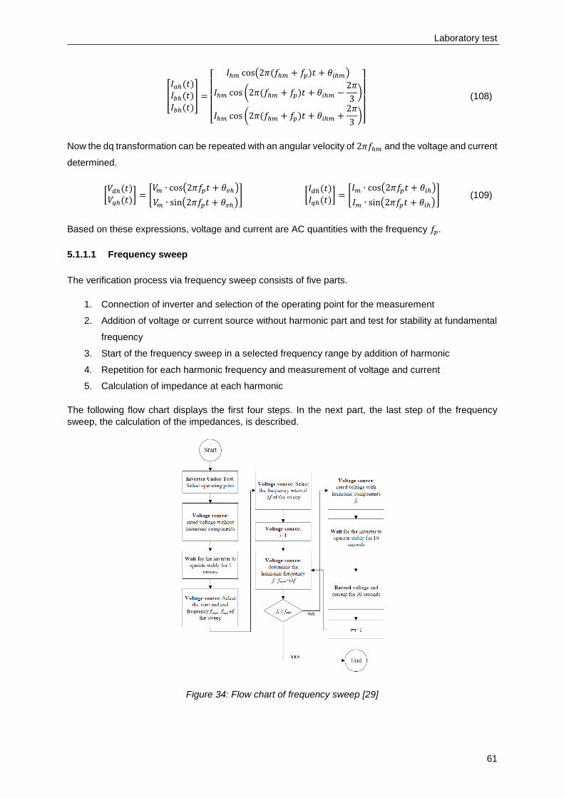
Laboratory test
61
[
𝐼𝑎ℎ(𝑡)𝐼𝑏ℎ(𝑡)
𝐼𝑏ℎ(𝑡)] =
[
𝐼ℎ𝑚 cos(2𝜋(𝑓ℎ𝑚 + 𝑓𝑝)𝑡 + 𝜃𝑖ℎ𝑚)
𝐼ℎ𝑚 cos (2𝜋(𝑓ℎ𝑚 + 𝑓𝑝)𝑡 + 𝜃𝑖ℎ𝑚 −2𝜋
3)
𝐼ℎ𝑚 cos (2𝜋(𝑓ℎ𝑚 + 𝑓𝑝)𝑡 + 𝜃𝑖ℎ𝑚 +2𝜋
3)]
(108)
Now the dq transformation can be repeated with an angular velocity of 2𝜋𝑓ℎ𝑚 and the voltage and current
determined.
[𝑉𝑑ℎ(𝑡)𝑉𝑞ℎ(𝑡)
] = [𝑉𝑚 ∙ cos(2𝜋𝑓𝑝𝑡 + 𝜃𝑣ℎ)
𝑉𝑚 ∙ sin(2𝜋𝑓𝑝𝑡 + 𝜃𝑣ℎ)] [
𝐼𝑑ℎ(𝑡)𝐼𝑞ℎ(𝑡)
] = [𝐼𝑚 ∙ cos(2𝜋𝑓𝑝𝑡 + 𝜃𝑖ℎ)
𝐼𝑚 ∙ sin(2𝜋𝑓𝑝𝑡 + 𝜃𝑖ℎ)] (109)
Based on these expressions, voltage and current are AC quantities with the frequency 𝑓𝑝.
5.1.1.1 Frequency sweep
The verification process via frequency sweep consists of five parts.
1. Connection of inverter and selection of the operating point for the measurement
2. Addition of voltage or current source without harmonic part and test for stability at fundamental
frequency
3. Start of the frequency sweep in a selected frequency range by addition of harmonic
4. Repetition for each harmonic frequency and measurement of voltage and current
5. Calculation of impedance at each harmonic
The following flow chart displays the first four steps. In the next part, the last step of the frequency
sweep, the calculation of the impedances, is described.
Figure 34: Flow chart of frequency sweep [29]

Laboratory test
62
5.1.1.2 Measurement evaluation in dq-domain
The measurement takes place in a stationary three-phase system; therefore, the relationship between
voltage and current is as follows:
[
𝑉𝑎(𝑡)𝑉𝑏(𝑡)
𝑉𝑐(𝑡)] = [
𝑍𝑎 0 00 𝑍𝑏 00 0 𝑐𝑎
] [
𝐼𝑎(𝑡)𝐼𝑏(𝑡)
𝐼𝑐(𝑡)] (110)
According to Formula (110), the impedance in stationary abc components of each phase is independent
of the other phases. After a transformation into Laplace-domain, this stays the same, however with a
transformation according to the small signal analysis into dq-domain; the impedance obtains a coupling
relationship [29].
[𝑉𝑑(𝑠)𝑉𝑞(𝑠)
] = [𝑍𝑑𝑑(𝑠) 𝑍𝑑𝑞(𝑠)
𝑍𝑞𝑑(𝑠) 𝑍𝑞𝑞(𝑠)] [
𝐼𝑑(𝑠)𝐼𝑞(𝑠)
] (111)
Now instead of calculating one impedance at each harmonic, four impedances should be computed. To
achieve this, two sets of linearly uncorrelated harmonic injections are necessary.
According to Formula (107) and (108), the angular velocity during the transformation has to be different
to the injected frequency. Correspondingly, 2𝜋(𝑓ℎ𝑚 ± 𝑓𝑝) would be a suitable way to determine the four
impedances [29].
[𝑉𝑑ℎ1(𝑠)𝑉𝑞ℎ1(𝑠)
] = [𝑍𝑑𝑑(𝑠) 𝑍𝑑𝑞(𝑠)
𝑍𝑞𝑑(𝑠) 𝑍𝑞𝑞(𝑠)] [
𝐼𝑑ℎ1(𝑠)𝐼𝑞ℎ1(𝑠)
] [𝑉𝑑ℎ2(𝑠)𝑉𝑞ℎ2(𝑠)
] = [𝑍𝑑𝑑(𝑠) 𝑍𝑑𝑞(𝑠)
𝑍𝑞𝑑(𝑠) 𝑍𝑞𝑞(𝑠)] [
𝐼𝑑ℎ2(𝑠)𝐼𝑞ℎ2(𝑠)
] (112)
With these two measurements, the four impedances in dq-domain can be measured.
[𝑍𝑑𝑑(𝑠) 𝑍𝑑𝑞(𝑠)
𝑍𝑞𝑑(𝑠) 𝑍𝑞𝑞(𝑠)] = [
𝑉𝑑ℎ1(𝑠) 𝑉𝑑ℎ2(𝑠)𝑉𝑞ℎ1(𝑠) 𝑉𝑞ℎ2(𝑠)
] [𝐼𝑑ℎ1(𝑠) 𝐼𝑑ℎ2(𝑠)𝐼𝑞ℎ1(𝑠) 𝐼𝑞ℎ2(𝑠)
]−1
(113)
Now again the influence of the inverter current 𝐼𝑟𝑒𝑓 has to be filtered out with a Band stop filter and finally
the accurate impedances in dq-domain can be calculated [29].
Figure 35: Schematic of the calculation process [29]
After calculating the four impedances for each harmonic, a plot of the impedance as a function of the
used harmonics is a useful summary of the frequency sweep. From this, the stability criterion can be
deployed and via the negative part of the admittance of each dq component unstable frequency ranges
illustrated.

Laboratory test
63
5.1.2 Results of frequency sweeps
Using the calculation scheme presented in the previous chapter, a frequency sweep of the real world
inverters as well as of the simulation models of Simulink is conducted. Afterwards, the values can be
compared in a diagram and a first statement about the basic stability can be given. A frequency range
from 150 to 5000 Hz is investigated.
5.1.2.1 Frequency sweeps of real world inverters
During the frequency sweep of the inverters, they are switched on in the PHIL laboratory and the
corresponding measurement data is obtained.
Table 15: Technical Data Inverter 1 and Inverter 2
Inverter 1: Inverter 2:
Input:
Start Voltage 200V Start Voltage 620 V
MPPT Operating
Voltage Range 200 V – 1000 V
MPPT Operating
Voltage Range 591 V – 1300 V
Output:
Nominal AC Active
Power 100 kW Rated Output 92 kVA
Max. THD < 3 % Max. THD < 3 %
Rated Current 144.4 V @ 400 V Rated Current 3 x 132.3 A
Measurement setup:
To operate an inverter, a DC and an AC voltage are required. The DC voltage comes from the source,
in this case the photovoltaic system, and the AC voltage is the link to the grid.
Since there is no real photovoltaic panel to generate the DC voltage, this is replaced in the lab with a
power amplifier (PA). This PA generates the necessary DC voltage for the inverter. The DC voltage of
both inverters is set to UDC = 700 V. The AC voltage is supplied via a second PA. This PA generates a
three-phase voltage with an amplitude of Urms, p-p = 400 V which equals Urms, p-n = 325 V. Both inverters
are set to an operating point of 8 MW.
Then a harmonic current is additionally fed in and a three-phase current and voltage measurement is
carried out. The transformer on DC side of Figure 36 decouples the ground connection, since in reality
the photovoltaic installation also does not have the same ground potential. The magnitudes of the
injecting voltage are matched to the PAs of the laboratory. This makes no difference to the impedance
characteristics, as these are not dependent on the output current and voltage.

Laboratory test
64
50 A gG
~
~
Test InverterInverter Rectifier
Laboratory
PE
(PA1)(PA2)DC+
DC-
N
L1
L2
L3
PE
Public grid
Test grid
Test grid 50 A gG
N
L1
L2
L3
PE
U5
U8
V8
U1
U4
V4
W4W8
V5
W5
V1
W1
~
N
L1
L2
L3
PE
RTSRTS Recorder
Voltage
measure
ment
Current
measure
ment
Figure 36: Laboratory setup frequency sweep
5.1.2.2 Frequency sweep of grid model
To make the frequency sweep of the grid model and measure the grid impedance, a current source is
placed at the location of the inverters. The current source feeds in the additional current and calculates
the values of the grid impedance for each harmonic current via a dq-transformation.
Figure 37: Simulation setup for frequency sweep

Laboratory test
65
The current source consists of two blocks in Simulink. Block 1 contains the measuring device in which
the transformation is carried out according to the verification process, and Block 2 consists of the
reconstruction of a three-phase current source with parallel internal resistors. Block 1 is shown in the
picture below for better understanding. The amplitude is determined on the basis of the maximum values
of the current from the field test according to the following formula. Five percent of the base current
amplitude is assumed and a ratio of 2:1 between the d and q components is adopted.
|𝐼5%| = √𝐼𝑑2 + 𝐼𝑞
2 (114)
Figure 38: Measurement block
5.1.2.3 Frequency sweep results
The results of the frequency sweep are divided into two parts. First, the inverters alone are considered
and their behaviour is discussed. Then the grid impedance is added in a common diagram and the result
is explained.

Laboratory test
66
Frequency sweep of real world inverters:
For the results of the frequency sweep of the real world inverters, the impedances in the dq-domain of
the inverters are considered first and then the real parts of the admittance of the inverter. At the points
where the real part of the admittance is negative, there is negative damping and instability in the event
of resonance in the network.
Z2Z 1
Comparison of Zdd, Zdq, Zqd and Zqq of both inverters
Figure 39: Comparison of inverter impedance of inverter 1 and 2
In Figure 39 the inverter impedance of the two tested inverters is displayed. As can be seen, the
behaviour of both inverters is very similar over the selected frequency range, with inverter 2 generally
having a lower impedance.
Y2Y 1
Comparison of Real part of Ydd, Ydq, Yqd and Yqq of both inverters
Figure 40: Comparison of inverter admittance of inverter 1 and 2

Laboratory test
67
The focus is on the dd and qq components as they are more expressive than the coupling components.
Due to the lower impedance of inverter 2, its real part of the admittance is generally higher than that of
inverter 1 and there are larger ranges in which the real part is greater than zero. If the GNC is used,
inverter 2 has a more stable internal behaviour. This could be due to a slower control of the inverter.
However, this slower behaviour results in poor control in the event of sudden errors such as a fault ride
through.
Frequency sweep of simulated grid impedance:
In the frequency sweep of the grid model, a passive behaviour of the impedance is generally assumed
and therefore only the impedance is shown.
Z grid,2TZ grid,1T
Comparison of Zdd, Zdq, Zqd and Zqq of the grid impedances with 1 and 2 transformers
Figure 41: Comparison of grid impedance of 1 and 2 transformers
In Figure 41, the grid impedance is plotted for an operation with one transformer in the photovoltaic
installation and compared to the grid impedance when using two transformers connected in parallel. As
can be seen, the green line representing the grid impedance with two transformers is slightly smaller at
all points. This behaviour makes sense, as the resistance value is reduced when impedances are
connected in parallel.

Laboratory test
68
The figure below shows the comparison between the inverter impedances and the grid impedance when
operated with only one transformer of the photovoltaic system.
The pink line represents the grid impedance and it can be seen that the grid impedance is always lower
than the inverter impedances. This behaviour follows the stability criterion very well, which means that
the entire system is stable when the inverter is connected. The difference in amplitude at the point with
the smallest distance is about 15 dB, which corresponds to a resistance value of 5.62 Ω and provides a
large enough distance between the curves.
Comparison of Zdd, Zdq, Zqd and Zqq of both inverters and grid impedance
Z2Z 1 Zgrid,1T
Figure 42: Comparison of inverters to grid impedance of operation with 1 transformer

Laboratory test
69
Even with 2 parallel transformers and thus lower impedance, the inverter impedance of both inverters
remains greater than the grid impedance in all components of the dq-domain. Again the stability criterion
is followed very well, which means that the entire system is also stable when this inverter is connected.
The difference in amplitude at the point with the smallest distance is about 10 dB, which corresponds to
a resistance value of 3.16 Ω and provides a large enough distance between the curves.
Comparison of Zdd, Zdq, Zqd and Zqq of both inverters and grid impedance
Z2Z 1 Zgrid,2T
Figure 43: Comparison of inverters to grid impedance of operation with two transformers

Laboratory test
70
5.2 PHIL – test
In inverter-coupled power supply systems, the dynamic characteristics strongly depend on the
implemented control strategy. This fact has already been described in the previous pages by modelling
the small-signal equivalent circuit of the inverter power system. In order to carry out a realistic
examination of the entire system, a verification of the simulation can be carried out with so-called
hardware-in-the-loop test methods.
By using Power/Controller-Hardware-In-The-Loop (PHIL or CHIL) systems, complex system behaviour
during faults can be detected during planning. The grid connection behaviour of converter-coupled
systems is mapped in simulations and these simulation models then verified by realistic results using
power hardware-in-the-loop methods.
PHIL tests are used to carry out a realistic examination of the overall system. In a PHIL test, the network
and the generating system are evaluated in a real-time simulation (RTS). In this context, Real time
simulations means that all the needed parameters to control the system must be completely calculated
within a time step. Therefore, only the inverter has to be an actual hardware device while the rest of the
grid model can be simulated.
The results are then transferred to the tested inverter via a power amplifier (PA). The power amplifier
calculates for every time step the needed values and transmits the values back to the inverter. As a
result, the inverter behaves in this configuration in the same way as in a real environment. With a PHIL-
test, the system behaviour during large disturbances, like a three-phase fault can be examined, without
any stress for real world equipment [33].
Figure 44: Topology of a PHIL test [33]

Laboratory test
71
The setup of this master's thesis with a photovoltaic on the generation side and the inverter to be tested
changes the schematics. Since photovoltaic as a source does not change its voltage generation rapidly
and the target time constant is smaller than 1 second, it can be represented by a constant DC source,
which corresponds to a rectifier. A PA, generating a DC voltage, represents this rectifier.
Figure 45: Schematic of the PHIL test of this master thesis
The verification process of the stability analysis in this master thesis is based on [29] with power-
hardware-in-the-loop (PHIL) testing. In the document, a quick verification process for local and global
stability is explained. For a small signal stability analysis, the local stability is of interest.
5.2.1 Method description
For the PHIL test, four different programmes are used for control. First, the two PAs are switched on via
ACScontrol and the corresponding values for DC and AC voltage generation are set. The values are
adjusted to the same amplitudes as for the frequency sweep. UDC = 700 V and Urms, p-p = 400 V which
equals Urms, p-n = 325 V. Then the grid model with photovoltaic system can be imported via
Matlab/Simulink and the required current and voltage values connected to the inputs and outputs of the
RTS system dSpace by importing the Simulink programme into Configuration Desk. After the inputs and
outputs are linked, the file is compiled and an overview of the voltages and currents is created in Control
Desk for monitoring during the test. Via Control Desk, the variables of the Simulink file can be modified
during operation and thus the whole system can be controlled.
During the PHIL-test, the current from the inverter is increased with the multiplication by Igain to simulate
a much higher current than in reality possible. The inverter in the laboratory is set to 8 % of the rated
power, equalling P = 8 kW, to achieve the worst-case scenario for the test. During the test, Igain is
increased from 1 to 50 and the voltage and current recorded. Figure 46 shows this relation between
hardware and software.
Figure 46: Laboratory setup scheme in combination with RTS connection

Laboratory test
72
5.2.2 Laboratory setup
Based on the schematics above and [29], the laboratory set up of a PHIL laboratory needs two AC/DC
voltage power amplifiers, a set of real-time simulators and an integrated measurement and control
system. In the setup of the master thesis, PA1 simulates the voltage of the photovoltaic installation and
supplies the inverter to be tested with its DC source. PA2 supplies the three-phase voltage from the grid
and represents the connection to the grid. The inverter in the grey box is the real world inverter to be
tested. The transformer on DC side decouples the ground connection, since in reality the photovoltaic
installation also does not have the same ground potential.
50 A gG
~
~
Test InverterInverter Rectifier
Laboratory
PE
(PA1)(PA2)DC+
DC-
N
L1
L2
L3
PE
Public grid
Test grid
Test grid 50 A gG
N
L1
L2
L3
PE
U5
U8
V8
U1
U4
V4
W4W8
V5
W5
V1
W1
~
N
L1
L2
L3
PE
RTSRTS RecorderRecorder
Figure 47: Laboratory setup PHIL-test
The next picture shows the PHIL laboratory during the test with the test set-up. The computers control
the RTS system and all the necessary calculation programmes. The inverter represents the equipment
under test (EUT) and the power amplifiers are located behind the green box.
Figure 48: Picture of PHIL test in laboratory

Laboratory test
73
5.2.3 PHIL – test results
5.2.3.1 Integrity of PHIL-test
In a correct PHIL-test, the voltage increases as the current increases. To prove the correctness of the
PHIL-test, the RMS value over the entire test period is considered. If Igain is increased, U must also
increase accordingly.
Figure 49 describes this behaviour very well. As Igain increases, the voltage also increases, and as Igain
decreases, the voltage also decreases.
5.2.3.2 Results of PHIL-test
In the next two images, the stability of the entire system in the PHIL-test is considered.
Figure 50 represents the entire system with only one transformer for the photovoltaic system. Although,
as previously described, the voltage must increase with increasing Igain, it must not become unstable
and its value must only change in a small range.
On the left side of Figure 50 it is clearly visible that the current is increased and decreased again, but
the voltage remains approximately constant over the entire time. Since the system does not oscillate, it
can be deduced that the system remains stable with the inverter connected in the worst-case state and
the photovoltaic system switched on, even with a much higher photovoltaic feed-in.
The right side shows the voltage and current at the maximum value of Igain during a few periods. The
voltage has a fairly accurate sinusoidal shape while the current contains many harmonics. The current
contains these harmonics because the inverter is not operated at its rated power but only at 8 % of it. If
the power of the inverter is increased, the curves of the current also become more sinusoidal. This is
because an inverter always produces 3rd, 5th, and 7th order harmonics, but these are in comparison to
the fundamental voltage and current at rated power according to the THD specified in the data sheet.
Now only 8 % of the rated power is used and the harmonics are amplified with Igain.
Figure 49: Correctness of PHIL-test

Laboratory test
74
Figure 50: PHIL-test with grid model with 1 transformer
Figure 51 represents the entire system with 2 transformers connected in parallel.
On the left side of Figure 51 it is clearly visible that the current is increased and decreased again, but
the voltage remains approximately constant over the entire time. Since the system does not oscillate, it
can be deduced that the system remains stable with the inverter connected in the worst-case state and
the photovoltaic system switched on, even with a much higher photovoltaic feed-in. Here, a longer time
interval is maintained between the increases of Igain than in the previous picture.
The same behaviour as with Figure 50 can be observed in the two images on the right.
Figure 51: PHIL-test with grid model with 2 transformers

Summary and findings
75
6 Summary and findings
6.1 Summary
In this master's thesis, the behaviour of a photovoltaic system is investigated when it is connected via
an inverter to an industrial grid at 6 kV voltage level.
First, a grid simulation is designed in Simulink on the basis of the construction plans and then validated
with a field test. During the field test of the industrial grid, a voltage and current measurement is carried
out on each feeder and on the main busbar. After the verification with the results of the field test, it has
been established that the simulation agrees very well with the values of reality. Thus, all subsequent
considerations with the simulation lead to realistic results when adding a photovoltaic model.
Two types of instabilities are investigated for the industry grid. The first type of instability originates from
the steady state and describes the instabilities that are generated due to the existing grid in one
operating situation. Here only the voltage stability is examined in order to determine whether an
undesirable voltage increase in the industrial grid would already occur with the planned power
generation by the photovoltaic installation.
In the process, the limits of the maximum permitted voltage increase are determined by TOR-D2 and
IEC 61000-2-4 and the formulas for voltage and current are defined based on the standards. It turns out
that the feed-in of 8 MW of the photovoltaic installation only increases the voltage by 1.35 % at the main
busbar of the industrial grid, which is far from the maximum permissible 10 %. Thus, it can be concluded
from the steady state analysis that the power increase in the industrial grid caused by the photovoltaic
installation alone will not lead to any problems, but that the correct cable cross-sections should be
ensured for the connecting lines to the planned photovoltaic system.
The second source of instability is described by the transient case. Here, instabilities are investigated
that arise due to the control algorithm as well as the dimensions of the inverter itself. In the course of
the analysis, the impedance-based approach and the generalized Nyquist criterion provide an
appropriate method for checking the stability of the individual components as well as the connection of
all components.
The grid system is divided into two subsystems, one consisting of all components up to the connection
point of the inverter and the second consisting of all components from the connection point of the inverter
to the photovoltaic installation. Based on the separation of the systems, the impedance of these two
subsystems can be calculated and their frequency response over a fixed frequency range observed by
applying the frequency sweeping algorithm. Two inverters from different manufacturers that are suitable
for building the photovoltaic system are reviewed in a laboratory test. A difference in the impedance of
the inverters can be observed, which indicates that the controller and the components of the inverters
are regulated differently.

Summary and findings
76
The simulation of the industrial grid is also subjected to a frequency sweep in the same frequency range.
For this, a current source is placed at the connection point of the inverter, which produces a harmonic
that is superimposed on the fundamental current. With the frequency behaviour of the inverters and the
grid obtained, a comparison of the curves can now be carried out and the impedance examined
according to the stability criterion.
First, the impedances are considered individually and the real part of the admittance of the individual
components is analysed. According to the stability criterion, a component/system is stable at a certain
frequency if the real part of the admittance at this frequency is greater than zero. Since both inverters
have negative real parts, the inverters have an instability at these frequency ranges according to this
method. If now a resonance would occur from the grid impedance exactly at this frequency, the inverter
would act like a resonance source and amplify this resonance by a negative damping. This would lead
to a higher current load in the grid, which could overload the equipment.
Therefore, it must be determined whether the ratio between inverter impedance and grid impedance
fulfils the stability criterion. This comparison corresponds to the ratio between inverter impedance and
grid impedance over the entire frequency range, which is also called short circuit ratio. The short circuit
ratio provides information about the stability of a grid. The higher this ratio, the more stable and secure
the grid, and the less likely it is that harmonics will occur in the grid or that grid operation will be disrupted.
By comparing the inverter impedance to the grid impedance, it can be determined; that the grid
impedance is consistently lower than the inverter impedance by at least a factor of 10, resulting in a
sufficient reserve between the two curves. Accordingly, the grid should not have any problems when
connected to the inverter.
In the power-hardware-in-the-loop test, all three components, namely photovoltaic cell, inverter and grid,
are tested together to obtain the overall system behaviour. Here, the simulation of the grid and the
photovoltaic system is connected to the real world inverter via a real-time system, whereby the inverter
behaves as if the grid and the photovoltaic panels are real hardware. Thus, the inverter also reacts as
if it is in real grid operation. In the power-hardware-in-the-loop test, the inverter is operated in worst-
case, which means that it is not operated at rated power but only at a small percentage of its rated
power. Thus, it can be assumed that if the worst-case functionality is working correctly, it will also ensure
the best-case functionality is provided. In addition, the current of the inverter is increased by the factor
Igain to a value that would not be possible in reality to test the behaviour of the inverter. During the tests,
both inverters showed no difficulties of stability when connected to the simulated industrial grid as well
as to the simulated photovoltaic installation, thus proving the overall system stability.
The industrial grid in connection with the photovoltaic panels and the inverter has thus successfully
completed three stability tests, the steady-state test according to IEC 61000-2-4, the frequency sweeps
based on the stability theory and the power-hardware-in-the-loop test. The voltage increase due to the
one connected photovoltaic system does not increase needlessly, the system divided into subsystems
has a stable behaviour up to 5000 Hz and the total system with connection of grid, inverter and
photovoltaic is stable.

Summary and findings
77
6.2 Outlook
Due to time constraints, only the models for an ideally symmetrical three-phase grid are carried out in
the master's thesis. Therefore, the differences in the models for an asymmetrical grid would be of
interest.
In addition, the resulting splitting into a positive sequence and a negative sequence and thus the
following influences the d and q components.
Also, a comparison between the impedance curves of the frequency sweep between inverter model and
real inverter would be interesting to be able to map the model of the inverter correctly via backwards
engineering.
These points can be discussed in a following doctoral thesis.

Bibliography
78
7 Bibliography
[1] E. T. D. N. a. R. M. J. R. Aguero, “Modernizing the Grid: Challenges and Opportunities for a Sustainable Future,” IEEE Power and Energy Magazine, pp. vol. 15, no. 3, pp. 74-83, May-June 2017.
[2] X. W. a. F. Blaabjerg, “Harmonic Stability in Power Electronic-Based Power Systems: Concept, Modeling, and Analysis,” IEEE Transactions on Smart Grid, pp. vol. 10, no. 3, pp, My 2019.
[3] R. S. L. F. X. L. Q. C. a. Y. Z. Z. Zhang, “Hardware-in-the-loop Based Grid Compatibility Test for Power Electronics Interface,” 2019 20th International Scientific Conference on Electric Power Engineering (EPE), pp. pp. 1-6, 2019.
[4] IEC TS 63102:2021.
[5] R.-C. L. C.-Y. C. S.-Y. C. J.-H. Teng, “Harmonic current predictors for wind turbines,” Energies, pp. 1314-1328, 2013.
[6] H. T. F. B. X. W. Z. H. a. S. G. H. Hu, “Train–Network Interactions and Stability Evaluation in High-Speed Railways–Part I: Phenomena and Modeling,” IEEE Transactions on Power Electronics, vol. 33, no. 6, pp. 4627-4642, 2018.
[7] C. R. P. W. S. H. N. Z. X. H. M. Chen, “Harmonic modelling and prediction of high speed electric train based on non-parametric confidence interval estimation method,” Int J Electr Power Energy Syst, vol. 87, pp. 176-186, 2017.
[8] E. S. E. Vasanasong, “The prediction of net harmonic currents produced by large numbers of residential PV inverters: Sydney Olympic village case study,” Ninth international conference on harmonics and quality of power, vol. 1, pp. 116-121, 2000.
[9] F. M. V. R. H.A.Pereira, “Harmonic current prediction by impedance modeling of grid-tied inverters: A 1.4 MW PV plant case study,” International Journal of Electrical Power & Energy Systems, vol. 93, pp. 30-38, 2017.
[10] J. J. A. A. a. T. S. T. Messo, “Time and frequency-domain evidence on power quality issues caused by grid-connected three-phase photovoltaic inverters,” 2014 16th European Conference on Power Electronics and Applications, pp. 1-9, 2014.
[11] P. Kundur, Power System Stability and Control, New York, 1994.
[12] W. Cao, Impedance-Based Stability Analysis and Controller Design of, Tennessee, 2017.
[13] M. M. K. Z. X. Qianjin Zhang, “Stability problems of PV inverter in weak grid: a review,” IET Power Electronics, vol. 13, no. 11, pp. 2165-2174, 2020.
[14] W. X. a. B. F. Wang Y., “Harmonic instability assessment using state-space modeling and participation analysis in inverter-fed power systems,” IEEE Trans. Power Electron., pp. 806-816, 2017.
[15] V. G. a. C. M. Guzman R., “Variable structure control for three-phase LCL-filtered inverters using a reduced converter model,” IEEE Trans. Ind. Electron., pp. 5-15, 2018.
[16] G. A. I. R. C. T. R. B. a. B. C. P. E. I. Batzelis, “A State-Space Dynamic Model for Photovoltaic Systems With Full Ancillary Services Support,” IEEE Transactions on Sustainable Energy, vol. 10, no. 3, pp. 1399-1409, 2019.
[17] E. V. M. C. G. S. 1. S. 1. A. G. F. D. S. G. L. P. M. P. F. B. Giovanni Nobile, “Performance Assessment of Large Photovoltaic (PV) Plants Using an Integrated State-Space Average Modeling Approach,” Energies, vol. 13, 2020.
[18] J. Sun, “Impedance-Based Stability Criterion for Grid-Connected Inverters,” IEEE TRANSACTIONS ON POWER ELECTRONICS, vol. 26, no. 11, 2011.
[19] C. G. H. R. A. R. L. F. Ziqian Zhang, “Resonance Instability of Photovoltaic E-Bike Charging Stations: Control Parameters Analysis, Modeling and Experiment,” Applied Sciences, 2019.
[20] A. A. R. L. a. T. M. M. Berg, “Small-Signal Analysis of Photovoltaic Inverter With Impedance-Compensated Phase-Locked Loop in Weak Grid,” IEEE Transactions on Energy Conversion, vol. 35, no. 1, pp. 347-355, 2020.

Bibliography
79
[21] Q. Z. W. M. a. S. G. X. Zhang, “Impedance-based local stability criterion for standalone photovoltaic-battery hybrid system,” 2015 IEEE 6th International Symposium on Power Electronics for Distributed Generation Systems (PEDG), pp. 1-6, 2015.
[22] B. D. a. L. F. Mao H., “Novel reduced-order small-signal model of a three-phase PWM rectifier and its application in control design and system analysis,” IEEE Trans. Power Electron., pp. 511-521, 1998.
[23] a. B. Z. Sun J., “Input impedance modeling of single-phase PFC by the method of harmonic linearization,” IEEE Appl. Power Electron. Conf., Austin, TX, USA, 2008, pp. 1188-1194, 2008.
[24] S. A. a. V. G. Mattavelli P., “SSR analysis with dynamic phasor model of thyristor controlled series capacitor,” IEEE Trans. Power Systems, vol. 14, pp. 200-208, 1999.
[25] a. S. J. Cespedesand M., “Renewable energy system instability involving grid-parallel inverters,” IEEE Appl. Power Electron. Conf., Washington, DC, USA, 2009, pp. 1971-1977, 2009.
[26] W. X. a. B. F. Bakhshizadeh M., “Couplings in phase domain impedance modeling of grid-connected converters,” IEEE Trans. Power Electron., vol. 31, pp. 6792-6796, 2016.
[27] a. S. J. Cespedes M., “Impedance modeling and analysis of grid-connected voltage-source converters,” IEEE Trans. Power Electron., vol. 29, pp. 1254-1261, 2014.
[28] B. J. a. G. J. Baimel D., “Dynamic modeling of networks, microgrids, and renewable sources in the dq0 reference frame: A survey,” IEEE Access, vol. 2017, no. 5, pp. 21323-21335, 2017.
[29] Z. Zhang, Test Guideline and Test Process of Power Hardware-in-the-Loop Test, Graz: TU Graz – Institut für Elektrische Anlagen und Netze, 2020.
[30] E-Control, Technische und organisatorische Regeln für Betreiber und Benutzer von Netzen - Teil D2.
[31] IEC 61000-2-4.
[32] P. C. K. M. G. A. M. S. S. IEEE, “Experiences with Wind Power Plants with Low SCR,” IEEE PES General Meeting, 2015.
[33] Z. Zhang, Power Electronics for Power Engineering, Technical University of Graz, 2020.
[34] S. C. Gupta, “Phase-Locked Loops,” Proceedings of the IEEE, vol. 63, no. 2, 1975.
[35] F. Blaabjerg, Control of Power Electronic Converters and Systems, 2021.
[36] F. H.A.Pereiraa, “Harmonic current prediction by impedance modeling of grid-tied inverters: A 1.4 MW PV plant case study”.

List of figures
80
8 List of figures
Figure 1: Grid single-line diagram ........................................................................................................... 7
Figure 2: Simulation in Simulink .............................................................................................................. 8
Figure 3: Simulation of the photovoltaic system .................................................................................... 12
Figure 4: (a) Single-phase equivalent circuit (b) equivalent circuit (c) phasor diagram of currents and
voltages ................................................................................................................................................. 20
Figure 5: Impedance-based equivalent circuit ....................................................................................... 24
Figure 6: Control circuit ......................................................................................................................... 25
Figure 7: Nyquist plot of a passive system [12] ..................................................................................... 26
Figure 8: Inverter model [33] ................................................................................................................. 27
Figure 9: SSM of PLL ............................................................................................................................ 32
Figure 10: Control circuit of SSM model: (a) without PLL (b): with PLL ................................................ 32
Figure 11: PLL phasor diagram ............................................................................................................. 33
Figure 12: Analytical model comparison impedance result ................................................................... 40
Figure 13: Analytical model comparison real part of admittance result................................................. 41
Figure 14: Analytical model with PLL impedance result different Padè orders ..................................... 42
Figure 15: Analytical model with PLL real part of admittance result different Padè orders................... 42
Figure 16: Comparison of analytical model with, without PLL and PV model impedance results ........ 43
Figure 17: Comparison of analytical model with, without PLL and PV model real part of admittance .. 43
Figure 18: Grid with photovoltaic system and added capacitance ........................................................ 44
Figure 19: Comparison of fr ................................................................................................................... 44
Figure 20: Current to the grid before and after connection case 1 ........................................................ 45
Figure 21: Vdq and Idq of inverter before and after connection case 1 ................................................... 45
Figure 22: Current to the grid before and after connection case 2 ........................................................ 46
Figure 23: Vdq and Idq of inverter before and after connection case 2 ................................................... 46
Figure 24: New controller parameters at Iabc ......................................................................................... 47
Figure 25: New controller parameters at Vdq and Idq ............................................................................. 48
Figure 26: Measuring set-up for the field test (single-line scheme) ...................................................... 49
Figure 27: Measuring set-up in reality ................................................................................................... 50
Figure 28: (a) Curves of U, I, P and Q (b) zoom to four periods ........................................................... 51
Figure 29: (a) Harmonics of 3rd, 5th, 7th (b) Harmonics of 11th, 13th (c) Harmonics of 23rd, 25th ............ 51
Figure 30: (a) Curves of U, I, P and Q (b) zoom to four periods ........................................................... 52
Figure 31: (a) Harmonics of 3rd, 5th, 7th (b) Harmonics of 11th, 13th (c) Harmonics of 23rd, 25th ............ 53
Figure 32: Voltage and current over time MV23.................................................................................... 56
Figure 33: Voltage and current over time MV24.................................................................................... 57
Figure 34: Flow chart of frequency sweep [29] ..................................................................................... 61
Figure 35: Schematic of the calculation process [29] ............................................................................ 62
Figure 36: Laboratory setup frequency sweep ...................................................................................... 64
Figure 37: Simulation setup for frequency sweep ................................................................................. 64

List of tables
81
Figure 38: Measurement block .............................................................................................................. 65
Figure 39: Comparison of inverter impedance of inverter 1 and 2 ........................................................ 66
Figure 40: Comparison of inverter admittance of inverter 1 and 2 ........................................................ 66
Figure 41: Comparison of grid impedance of 1 and 2 transformers ...................................................... 67
Figure 42: Comparison of inverters to grid impedance of operation with 1 transformer ....................... 68
Figure 43: Comparison of inverters to grid impedance of operation with two transformers .................. 69
Figure 44: Topology of a PHIL test [33] ................................................................................................. 70
Figure 45: Schematic of the PHIL test of this master thesis ................................................................. 71
Figure 46: Laboratory setup scheme in combination with RTS connection .......................................... 71
Figure 47: Laboratory setup PHIL-test .................................................................................................. 72
Figure 48: Picture of PHIL test in laboratory ......................................................................................... 72
Figure 49: Correctness of PHIL-test ...................................................................................................... 73
Figure 50: PHIL-test with grid model with 1 transformer ....................................................................... 74
Figure 51: PHIL-test with grid model with 2 transformers ..................................................................... 74
9 List of tables
Table 1: Cable values ............................................................................................................................ 10
Table 2: Values for transformer 1 .......................................................................................................... 11
Table 3: Values for transformer 2 .......................................................................................................... 11
Table 4: Values for transformer 3 .......................................................................................................... 12
Table 5: IEC 61000-2-4 harmonic limits ................................................................................................ 13
Table 6: TOR-D2 harmonic current limits .............................................................................................. 14
Table 7: Investigated states ................................................................................................................... 17
Table 8: IEC 61000-2-4 summary of maximum allowable voltage values ............................................ 18
Table 9: TOR-D2 summary of maximum allowable current values ....................................................... 18
Table 10: Steady-state harmonic voltage summary .............................................................................. 19
Table 11: Data of transformer 1............................................................................................................. 21
Table 12: Comparison of simulation and measurement MV23 ............................................................. 54
Table 13: Comparison of simulation and measurement MV24 ............................................................. 55
Table 14: Measurement and simulation with PV ................................................................................... 58
Table 15: Technical Data Inverter 1 and Inverter 2 ............................................................................... 63