Investigating the Stability of Viscoelastic Stagnation

Flows in T-shaped Microchannels

J. Soulagesa,∗, M. S. N. Oliveirab, P. C. Sousab, M. A. Alvesb, and

G. H. McKinleya,∗

aHatsopoulos Microfluids Laboratory, Department of Mechanical Engineering,

Massachusetts Institute of Technology, Cambridge, MA 02139, USA

bFaculdade de Engenharia da Universidade do Porto, Departamento de Engenharia

Quımica, Centro de Estudos de Fenomenos de Transporte, Rua Dr. Roberto Frias,

4200-465 Porto, Portugal

Preprint submitted to Elsevier Science 5 June 2009

Abstract

We investigate the stability of steady planar stagnation flows of a dilute polyethylene

oxide (PEO) solution using T-shaped microchannels. The precise flow rate control and

well-defined geometries achievable with microfluidic fabrication technologies enable us to

make detailed observations of the onset of elastically-driven flow asymmetries in steady

flows with strong planar elongational characteristics. We consider two different stagnation

flow geometries; corresponding to T-shaped microchannels with, and without, a recircu-

lating cavity region. In the former case, the stagnation point is located on a free stream-

line, whereas in the absence of a recirculating cavity the stagnation point at the separating

streamline is pinned at the confining wall of the microchannel. The kinematic differences

in these two configurations affect the resulting polymeric stress fields and control the criti-

cal conditions and spatiotemporal dynamics of the resulting viscoelastic flow instability. In

the free stagnation point flow, a strand of highly-oriented polymeric material is formed

in the region of strong planar extensional flow. This leads toa symmetry-breaking bi-

furcation at moderate Weissenberg numbers followed by the onset of three-dimensional

flow at high Weissenberg numbers, which can be visualized using streak-imaging and

microparticle image velocimetry. When the stagnation point is pinned at the wall this

symmetry-breaking transition is suppressed and the flow transitions directly to a three-

dimensional time-dependent flow at an intermediate flow rate. The spatial characteristics

of these purely elastic flow transitions are compared quantitatively to the predictions of

two-dimensional viscoelastic numerical simulations using a single-mode simplified Phan-

Thien-Tanner (SPTT) model.

Key words: Microfluidics; Polyethylene oxide (PEO); Particle image velocimetry; Flow

instability; Symmetry-breaking bifurcation; Simplified Phan-Thien-Tanner model.

∗ Corresponding author. E-mail addresses: soulages@mit.edu (Johannes Soulages),

2

1 Introduction

The continuous miniaturization of flow geometries achievable through microflu-

idic fabrication techniques has multiple processing advantages including decreased

manufacturing costs, fast response times, minimal fluid volumes, precise control

over multiphase morphology and increased separation efficiency [1, 2]. In particu-

lar, microfluidic technology is very relevant to industriesassociated with genomics,

construction of biosensors and lab-on-a-chip diagnosticsin addition to ink-jet print-

ing [3–5]. Microfluidic technology has also shown its remarkable potential in the

field of biochemical analysis and constitutes a valuable tool for separation or mix-

ing, automation and integration of complex chemical and biological assays [6, 7].

In these applications, many of the fluids of interest are non-Newtonian in character

and understanding their flow behavior at the microscale is important to the design

and optimization of the resulting microfluidic devices.

The wide range of deformation rates that can be attained (through precise control of

the imposed fluid flow rate and the small characteristic length-scales of the geom-

etry) coupled with the ability to directly image the resulting flow field also make

microfluidic devices good platforms for constructing rheometers and flow cham-

bers that enable a systematic investigation of non-Newtonian effects. An overview

of several canonical flow types and the challenges associated with quantitative mi-

crofluidic rheometry can be found in [8]. In the present work,we focus on two

different T-shaped microchannels that are specially constructed to enable an in-

vestigation of viscoelastic effects on the stability of planar elongation flows. The

channels are fabricated in such a way that the character of the stagnation flow near

the separating streamline is modified by the presence, or absence, of a rectangu-

gareth@mit.edu (Gareth H. McKinley).

3

lar cavity. The recirculating flow in this cavity is separated from the free stream

by a bounding streamline and this changes the local character of the flow near the

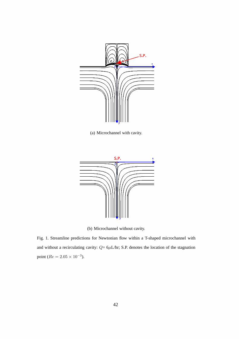
stagnation point. To illustrate this graphically, we show in Figures 1(a) and 1(b)

computational predictions of the expected streamlines forsteady viscous flow of a

Newtonian fluid within a T-shaped microchannel with and without a recirculating

cavity atRe = 2.05×10−3. In the absence of the cavity, the stagnation point is lo-

cated along the symmetry line at the intersection point of the channel sidewall and

the separating streamline. As a consequence of the no-slip boundary condition and

continuity, the local velocity vector and all velocity gradients are zero at the stag-

nation point. By contrast, the presence of the cavity and theunconstrained dividing

streamline leads to a non-zero velocity gradient at the origin in Fig. 1(a) and the

stagnation point is free to move. If we denote the location ofthe pinned stagnation

point as the origin of the laboratory frame (as shown in Fig. 1(b)) then the pres-

ence of a free or “unpinned” stagnation point leads to a smallvertical displacement

towards negativey-values inside the cavity.

Both of these flow geometries feature curved streamlines andgenerate a (nonho-

mogeneous) planar extensional flow near the stagnation point. These conditions can

promote purely elastic flow instabilities [9, 10]. The T-channel geometry has also

been suggested as a suitable geometry for constructing a microfluidic rheometer if

the total pressure drop associated with steady symmetric flow of a non-Newtonian

fluid is measured [11]. The presence, or absence, of the recirculating cavity thus

allows us to focus on the global kinematic consequences thatresult from fluid vis-

coelasticity and from local changes in the stagnation flow region. Furthermore, the

identical upstream flow conditions in each geometry resultsin a well-defined pre-

shearing history which can be important if a viscoelastic fluid is studied in place of a

simple viscous liquid. Similar elongational flows with “pinned” and “free” stagna-

4

tion points arise in the wakes of objects such as cylinders/spheres and behind rising

bubbles [12, 13]. In the case of a rising bubble, fluid elasticity leads to the formation

of a cusp and a symmetry-breaking instability that can be observed experimentally

[14] and studied computationally [15]. The unsteady Lagrangian nature of the flow

near the rising bubble however complicates the systematic experimental study of

the wake near a free stagnation point.

Creeping flows in, and past, cavities have been studied extensively at the macroscale.

Pan and Acrivos [16] explored the evolution in the vortex strengths as the cavity

depth was changed and Taneda [17] performed an extensive photographic study of

the effects of the cavity breadth to height ratio on the formation of vortices inside

a cavity using viscous Newtonian liquids such as silicone oil and glycerine. The

work of Perera et al. [18] is an example of early numerical work on the effect of

elasticity for steady 2D flow in macroscale L-shaped and T-shaped channels. They

showed that elasticity only leads to slight deviations in the streamline patterns at

low Reynold numbers compared to the Newtonian case. The study of Nishimura

and coworkers [19] represents an early combined experimental and numerical study

of 2D viscoelastic flow in T-shaped channels using streakline imaging. They studied

the effects of elasticity by comparing the flow patterns for aviscoelastic polyacry-

lamide aqueous solution and a Newtonian dextrose syrup seeded with aluminum

powder. They experimentally observed a lip vortex at the re-entrant channel cor-

ners in the flows of the polyacrylamide solution. Numerical simulations with the

upper-convected Maxwell model atWi ≤ 0.2 were able to capture qualitatively

the viscoelastic distortion in the streamlines, but not theformation of a lip vortex.

Binding et al. [20] also investigated viscoelastic creeping flow in a T-junction and

past a cavity. They showed that compared to the Newtonian symmetric behavior,

the flow of a highly elastic Boger fluid past a cavity clearly became asymmetric be-

5

yond a critical flow rate. Using the same flow geometry, they created a stagnation

flow by having flow in the two opposing arms of the T-junction. They observed the

formation of lip vortices in the case of the flow of a shear-thinnig polymer solu-

tion while such vortices were absent for the Boger fluid. In the present study, we

aim to characterize the onset of elastic instabilities in similar geometries but at the

microscale.

Utilizing microfluidic channels to explore such flows offersthe possibility of ex-

ploring new regimes of parameter space, that are not readilyaccessible in macroscale

experiments [21]. The relevant dimensionless groups used to characterize a vis-

coelastic stagnation flow are the Reynolds number (Re), the Weissenberg number

(Wi) and an elasticity number (El = Wi/Re). An appropriate Reynolds number

can be calculated according toRe = (ρV Dh)/(η0), whereDh represents the hy-

draulic diameter of the flow channel andρ andη0 represent the fluid density and

zero-shear rate viscosity, respectively. Viscoelastic effects in the geometry can be

characterized using a Weissenberg numberWi = λγ whereγ = V /ℓ is an appro-

priate estimate of the characteristic deformation rate based on the average velocity

at the channel inlet,V , and the relevant lengthscaleℓ controlling the kinematics of

the stagnation region. The elasticity numberEl = Wi/Re = λη0/(ρℓDh), defined

as the ratio of the Weissenberg to Reynolds number, is a measure of the relative im-

portance of elastic to inertial effects, and depends only onthe experimental geome-

try and the material properties of the fluid being studied. With the small geometric

length scales characteristic of microfluidic geometries itis possible to probe strong

elastic effects in the absence of inertial effects; for example in the micro-fabricated

planar contractions of Rodd et al. [21, 22], elasticity numbers as high asEl = 89

could be achieved.

Because inertial effects are small, microfluidic devices also provide good platforms

6

to study “purely elastic instabilities” that can arise fromthe combination of curved

streamlines and large tensile viscoelastic stresses [23, 24]. The time-dependent

three-dimensional flow that sometimes ensues following onset of a purely elastic

flow instability can greatly enhance the mixing efficiency ofa microfluidic device

at small Reynolds number [25]. There have been few studies todate that have sys-

tematically investigated the dynamics associated with these elastic nonlinearities

on the microscale [21, 26–30]. With microfluidic computing in mind, Groisman et

al. were the first to exploit elastic instabilities in designing a nonlinear fluid resistor,

a bistable flip-flop memory element [28] and a flow rectifier [29]. Reviews of ef-

forts made to develop nonlinear fluidic logic elements usingNewtonian fluids such

as water or air can be found in [31, 32].

The T-channel design considered in the present work is obviously closely con-

nected to the “cross-slot” configuration which has been usedextensively in rhe-

ological studies of steady planar elongation flow [8, 33, 34]. In either geometry,

the combination of streamline curvature and large extensional deformations near

the stagnation point may be anticipated to result in large viscoelastic effects within

the flow. The loss of symmetry in a microfluidic cross-slot flowat high flow rates

is evident in the micellar experiments of Pathak and Hudson [34]. Arratia et al.

have documented the existence of a purely elastic instabilities for the case of the

cross-slot flow of a polyacrylamide dilute solution [30]. They observed two distinct

flow regimes at very small Reynolds numbers (Re ≤ 10−2): a symmetry-breaking

bistable bifurcation forWi ≃ 4.5 followed by broadband temporal fluctuations at

Wi & 12.5. Very recently these observations of viscoelastic symmetry-breaking

have been validated numerically by Poole et al. [35]. By using the upper-convected

Maxwell model they demonstrated the purely elastic nature of the flow transition

and reported that inertia had a stabilizing effect, delaying the onset of the steady

7

asymmetric flow to higherWi.

In the present work we seek to compare, quantitatively, experimental observations

and numerical computations of this viscoelastic symmetry-breaking transition. By

selecting T-channels with, and without, recirculating cavities we can explore the

importance of the local planar elongational flow near a “free” and “pinned” stagna-

tion point, respectively. The experiments are performed with a well-characterized

dilute aqueous solution of monodisperse PEO and the 2D calculations are per-

formed using a prototypical nonlinear constitutive model with parameters selected

to fit the viscometric properties of the test fluid. In Section2, we describe the fab-

rication of the test geometries, the imaging techniques andthe characterization of

the test fluid rheology. In Section 3, we briefly describe the numerical method and

then investigate the magnitude of the “birefringent strand” that is generated in the

two different planar elongation flows. In Section 4, we compare streak-imaging

measurements and numerical calculations of the streamlines for each microfluidic

geometry as the flow rate (and corresponding Weissenberg number) is incremented.

In the presence of a recirculating cavity, a symmetry-breaking transition is observed

experimentally and predicted computationally at a critical Weissenberg number. By

contrast, in the absence of a cavity, the flow near the dividing streamline remains

stable and symmetric to substantially higher flow rates before losing stability to

three-dimensional and time-dependent perturbations.

2 Experimental

In order to perform quantitative comparisons between experimental measurements

and numerical computations, it is essential to carefully determine all geometri-

cal and rheological parameters as well as clearly define appropriate dimensionless

8

measures of elasticity and inertia.

2.1 Microfluidic Stagnation Flows and Dimensionless Groups

The appropriate Reynolds number for this pressure-driven channel flow is calcu-

lated according toRe = (ρQDh)/(hdη0), whereDh represents the hydraulic di-

ameter,Dh = 2dh/(d + h), h andd are respectively the channel width and depth

as shown in Fig. 2. The material propertiesρ andη0 represent the solution density

and zero-shear rate viscosity, respectively, and are givenin Table 1. We character-

ize the elastic effects in the stagnation flow using a Weissenberg number defined

asWi = λCaBERγ = λCaBERV /(h/2) = (2QλCaBER)/(dh2), whereλCaBER is the

relaxation time determined from CaBER measurements (c.f. Section 2.3),γ is the

shear rate based on the average velocity at the channel inlets, V = Q/(dh) and a

representative length scale for the local stagnation flow suggestsℓ = h/2. The elas-

ticity numberEl, defined as the ratio of the Weissenberg to Reynolds number, is a

measure of the relative importance of elastic to inertial effects:El = Wi/Re. El

depends only on the experimental geometry and the material properties of the inves-

tigated fluid. In our work, the elasticity numberEl= 8.61×102 is very large so that

the elastic stresses dominate compared to inertial effects. Thus, our flow geometries

allow us to probe elastically-driven flow transitions and instabilities that arise due

to the presence of bending streamlines and large tensile viscoelastic stresses in the

absence of inertia [23, 24].

9

2.2 Microchannel Geometry and Fabrication

The relevant variables and dimensions of the micro-fabricated channels used in this

study are given in Fig. 2 for the case of the microchannel witha recirculating cavity.

The working fluid is injected at the inlets (A) and (B) and exits the channel through

the outlet (C). The fluid is directed to the entrances of the central T-junction circled

in the figure by means of two entry channels of lengthL1=7 mm. It then enters

each side of the T-shaped region and travels a distanceL2=1 mm before reaching

the stagnation point (S.P.) region.

The channel widthh and depthd are both equal to 50µm. For the entire range of

Reynolds numbers investigated in this work, this distanceL2 is more than 30 times

larger than the entrance lengthLe needed to reach fully developed Newtonian flow,

which is given byLe = Dh[0.6/(1 + 0.035Re) + 0.056Re] = 30µm, where the

hydraulic diameterDh coincides with the channel widthh for our particular geom-

etry [36]. The square cavity has a length equal toh and the corners of the outflow

channel are rounded with a radiusR = 25µm in order to guarantee a smooth tran-

sition between the inflow and outflow regions. The T-shaped microchannels were

fabricated from polydimethylsiloxane (PDMS) using soft-lithography techniques

and SU-8 photoresist molds [37–40]. Light micrographs of the microchannels with

and without a cavity are shown in Figs. 3(a) and 3(b), respectively. As discussed in

Section 1, the two channel designs differ in the location of the stagnation point: in

the presence of the cavity it sits on a “free” streamline whereas it is pinned on the

wall of the channel without the recirculating cavity.

A detailed description of the microchannel fabrication procedure is given elsewhere

[41]. The use of a contrast enhancement material (CEM388SS,Shin-Etsu MicroSi)

allows us to achieve well-defined geometries as shown in Fig.4(a) with almost

10

perfectly-vertical channel sidewalls (the tapering angleis uniformly less than 5 as

illustrated in Fig. 4(b)).

2.3 Test Fluid Rheological Characterization

The test fluid used in the present experiments is a dilute polymer solution of a

high molecular weight polyethylene oxide (0.075 wt.%) witha relatively narrow

molecular weight distribution (PEO,Mw = 2 × 106 g/mol, polydispersity index

Mw/Mn = 1.13 [22], Aldrich) in a glycerol/water mixture (60/40 wt.%). The rhe-

ological properties of the PEO solution were characterizedin both steady shear

and transient uniaxial extension. The polymeric solution and solvent zero-shear

rate viscosities were obtained from viscometric experiments in a double gap Cou-

ette geometry using a controlled stress rheometer (AR-G2, TA Instruments). The

steady shear data were measured at 23C for shear rates in the range1 ≤ γ ≤

10, 000 s−1 and are presented in Fig. 5. The PEO solution has a zero-shearrate vis-

cosityη0 = 19.5 mPa s and is weakly shear thinning for shear ratesγ ≥ 15 s−1. This

gives a coarse estimate of a characteristic relaxation timeλ ≃ 1/15 s−1 = 67ms

which is in good agreement with the relaxation time determined from CaBER mea-

surements in Fig. 6. The zero-shear rate viscosity of the solvent isηS = 9.8 mPa s

resulting in a total polymeric contribution to the zero-shear rate viscosity ofηP =

9.7 mPa s. The predictions of the SPTT model are shown by the red dashed and

solid lines, respectively, forε = 0 (Oldroyd-B model) andε = 7.0 × 10−6.

Also represented in Fig. 5 are the lower and upper limits of the shear data based on

the rheometer torque transducer specifications and the onset of Taylor instabilities

as described in [21]. According to a linear stability analysis [42], the critical Taylor

number at the onset of inertial instabilities for a Newtonian fluid in the Couette

11

geometry is given byTacrit ≃ 2Re2 φ = 3400, whereRe denotes the Reynolds

number andφ = d/Rin is the ratio of the gap widthd and the radius of the inner

cylinderRin. The Reynolds number for circular Couette flow is defined asRe =

ρΩinRind/η(γ), whereΩin represents the angular velocity of the inner cylinder,ρ is

the density andη(γ) is the (shear-rate-dependent) viscosity of the PEO solution. For

Rin = 22 mm (outer radius of the rotor),d = 0.38 mm,ρ = 1196kg/m3, the criterion

for the onset of Taylor instabilities can be rewritten asη(γ) = 5.5 × 10−7 γ, where

η is in Pa s andγ in s−1. This equation is represented by the dashed line labeled (ii)

in Fig. 5.

The characteristic relaxation time of the solution was determined from capillary

breakup extensional rheometry (CaBER) measurements as illustrated in Fig. 6.

A thorough description of this technique can be found in [43–45]. Following the

nomenclature of [45], the CaBER geometrical configuration used in the present

study was such that the initial height wash0 = 2.11 mm (Λ0=h0/(2R0)= 0.35)

and the final aspect ratio wasΛf = 1.57, corresponding to an imposed step strain

of ǫ = ln(Λf/Λ0) = 1.50. In Fig. 6, the blue (thick) solid line represents the fit

to the measured evolution of the filament diameter using a single exponential de-

cay and based on the Oldroyd-B model [44]. The resulting relaxation time equals

λCaBER = 66 ± 4 ms.

Also shown in Fig. 6 are the results of the 1D calculations with the SPTT model.

This model (see Section 3.1 for details) contains a single nonlinear constitutive

parameter (ε) which controls the magnitude of strain-hardening in the extensional

viscosity of the fluid (ηE ≃ 2ηP /ε for smallε [46]). As the polymer chains in the

thinning thread approach full extension, the filament radius no longer thins expo-

nentially; but instead decreases linearly in time [47]. This deviation from exponen-

tial behavior allows us to determine a bound on the range of values ofε character-

12

izing the 0.075 wt.% PEO solution. From the data and simulations shown in Fig. 6,

it is clear that the PEO molecules are highly extensible with0 ≤ ε ≤ 7.0 × 10−6.

Any further increase inε restricts the region of exponential decay and reduces the

predicted time to breakup to unphysically small values.

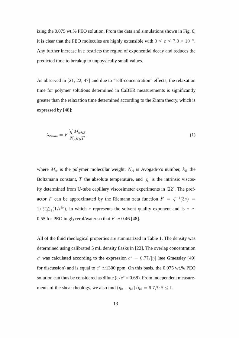
As observed in [21, 22, 47] and due to “self-concentration” effects, the relaxation

time for polymer solutions determined in CaBER measurements is significantly

greater than the relaxation time determined according to the Zimm theory, which is

expressed by [48]:

λZimm = F[η]MwηS

NAkBT, (1)

whereMw is the polymer molecular weight,NA is Avogadro’s number,kB the

Boltzmann constant,T the absolute temperature, and[η] is the intrinsic viscos-

ity determined from U-tube capillary viscosimeter experiments in [22]. The pref-

actor F can be approximated by the Riemann zeta functionF = ζ−1(3ν) =

1/∑

∞

i=1(1/i3ν), in which ν represents the solvent quality exponent and isν ≃

0.55 for PEO in glycerol/water so thatF ≃ 0.46 [48].

All of the fluid rheological properties are summarized in Table 1. The density was

determined using calibrated 5 mL density flasks in [22]. The overlap concentration

c⋆ was calculated according to the expressionc⋆ = 0.77/[η] (see Graessley [49]

for discussion) and is equal toc⋆ ≃1300 ppm. On this basis, the 0.075 wt.% PEO

solution can thus be considered as dilute (c/c⋆ = 0.68). From independent measure-

ments of the shear rheology, we also find(η0 − ηS)/ηS = 9.7/9.8 ≤ 1.

13

2.4 Flow Visualization

The microparticle image velocimetry experimental setup consists of a CCD camera

(mvBlueFOX-120a, Matrix Vision GmbH), an inverted microscope (Nikon, Eclipse

TE 2000-S) equipped with a G-2A filter cube (exciter, 535-550nm; dichroic, 565

nm; long-pass emitter, 590 nm) and an external continuous light source (mercury

lamp, illumination wavelength: 532 nm). The solution is fedto the channel inlets

using Tygon tubing by means of two twin syringe pumps (New EraPump Sys-

tems, Inc.) and two Hamilton gastight syringes (500µL, diameter: 3.26 mm). The

PEO solution is seeded with 1.1µm diameter fluorescent tracer particles (Nile Red,

Molecular Probes, Invitrogen; Ex/Em: 520/580 nm;cP = 0.02 wt.%), which are il-

luminated by the light source and imaged through the microscope objective (20×,

0.5 N.A.) onto the CCD array of the camera at a frame rate of 3.81 fps and exposure

time of about 250 ms.

Sodium dodecyl sulfate (SDS) from Sigma-Aldrich was added to the PEO solution

at a concentration ofcSDS = 0.1 wt.% in order to inhibit the fluorescent tracers from

sticking onto the polydimethylsiloxane microchannel walls. The addition of SDS

was shown to have a negligible influence on the value of the relaxation timeλCaBER

measured from CaBER experiments as well as on the values of both η0 andηS.

All of the streakline images presented in this work were recorded at the mid-plane

of the microchannel. The physical location of the mid-planewas determined ex-

perimentally by successively focusing the image of a fluorescent tracer adhered to

the top and bottom surfaces of the channel. The depth over which the tracers con-

tribute to the recorded streamlines is actually given by themeasurement depthδzm

14

[21, 22, 50] given by

δzm =3nλ0

(NA)2+ 2.16

dP

tan(θ)+ dP. (2)

In Eq. (2),λ0 represents the wavelength of the emitted light (λ0=580 nm),n is

the medium refractive index (watern=1.33),NA is the numerical aperture of the

objective lens,dP is the tracer diameter andθ is defined asθ = sin−1(NA/n).

Equation (2) is only valid fordP > e/M, wheree andM respectively denote the

minimum resolvable feature size (or the CCD camera pixel size: 7.4µm) and the

objective magnification. In our work,e/M= 0.37µm, which is very small com-

pared to the diameter of the tracer particles (1.1µm). The depth of measurement

can thus be determined from Eq. (2) and isδzm=14.5µm, which corresponds to

approximately 29 % of the total channel depth.

3 Numerical Method and Computational Meshes

3.1 Governing Equations and Numerical Method

In addition to the experimental measurements, we perform 2D-calculations to sim-

ulate the isothermal flow of the viscoelastic fluid through T-shaped microchannels

with and without the recirculating cavity. We use a fully-implicit finite-volume

method with a time-marching pressure-correction algorithm [51, 52] to solve the

equations of conservation of mass and momentum:

∇ · u= 0, (3)

ρ

[

∂u

∂t+ u · ∇u

]

=−∇p + ηS∇ ·[

∇u + (∇u)T]

+ ∇ · τ , (4)

15

together with an appropriate constitutive equation for thepolymeric component of

the extra-stress,τ . The numerical code used here has been applied extensively in

2D calculations [53, 54] and with axisymmetric geometries [55]. Additionally, it

has also been used for full three-dimensional (3D) simulations including those of

planar channels in which the depth of the channels is kept constant as is typical of

microfluidic fabrication [50, 56].

Regarding the boundary conditions, we imposed fully-developed velocity and stress

profiles at the inlets, Neumann boundary conditions at the outlet, and no-slip con-

ditions at the walls. Details of the implementation of boundary conditions can be

found in Oliveira et al. [51]. For the discretization of the equations, we use central

differences for the diffusive terms and the CUBISTA high-resolution scheme [57]

for the convective terms.

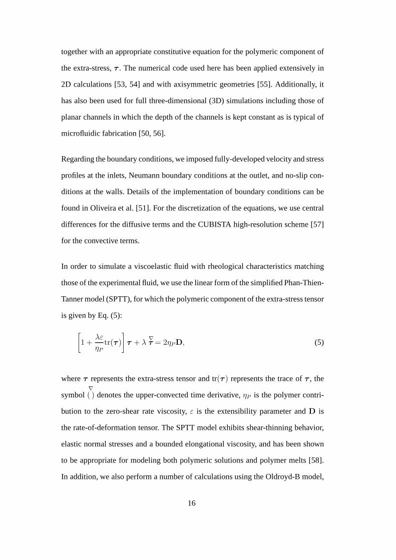
In order to simulate a viscoelastic fluid with rheological characteristics matching

those of the experimental fluid, we use the linear form of the simplified Phan-Thien-

Tanner model (SPTT), for which the polymeric component of the extra-stress tensor

is given by Eq. (5):

[

1 +λε

ηP

tr(τ )

]

τ + λ∇

τ = 2ηPD, (5)

whereτ represents the extra-stress tensor and tr(τ ) represents the trace ofτ , the

symbol∇

( ) denotes the upper-convected time derivative,ηP is the polymer contri-

bution to the zero-shear rate viscosity,ε is the extensibility parameter andD is

the rate-of-deformation tensor. The SPTT model exhibits shear-thinning behavior,

elastic normal stresses and a bounded elongational viscosity, and has been shown

to be appropriate for modeling both polymeric solutions andpolymer melts [58].

In addition, we also perform a number of calculations using the Oldroyd-B model,

16

which is a limiting case of the SPTT model that can be recovered whenε = 0.

To enhance numerical stability, we employ the log-conformation tensor approach

[59], as decribed in detail in Afonso et al. [60].

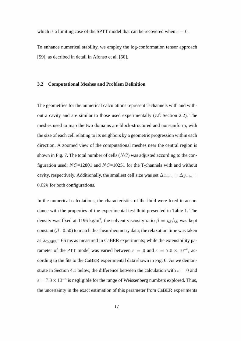
3.2 Computational Meshes and Problem Definition

The geometries for the numerical calculations represent T-channels with and with-

out a cavity and are similar to those used experimentally (c.f. Section 2.2). The

meshes used to map the two domains are block-structured and non-uniform, with

the size of each cell relating to its neighbors by a geometricprogression within each

direction. A zoomed view of the computational meshes near the central region is

shown in Fig. 7. The total number of cells (NC) was adjusted according to the con-

figuration used:NC=12801 andNC=10251 for the T-channels with and without

cavity, respectively. Additionally, the smallest cell size was set∆xmin = ∆ymin =

0.02h for both configurations.

In the numerical calculations, the characteristics of the fluid were fixed in accor-

dance with the properties of the experimental test fluid presented in Table 1. The

density was fixed at 1196 kg/m3, the solvent viscosity ratioβ = ηS/η0 was kept

constant (β= 0.50) to match the shear rheometry data; the relaxation time was taken

asλCaBER= 66 ms as measured in CaBER experiments; while the extensibility pa-

rameter of the PTT model was varied betweenε = 0 andε = 7.0 × 10−6, ac-

cording to the fits to the CaBER experimental data shown in Fig. 6. As we demon-

strate in Section 4.1 below, the difference between the calculation withε = 0 and

ε = 7.0× 10−6 is negligible for the range of Weissenberg numbers explored. Thus,

the uncertainty in the exact estimation of this parameter from CaBER experiments

17

is not critical in the present computations.

4 Results and Discussion

We first examine the influence of the extensibility parameterε on the streamlines

predicted by the SPTT model and subsequently analyze the stress field obtained

from 2D numerical simulations. We then compare the flow patterns obtained in

the T-shaped microchannels with and without a recirculating cavity for both the

viscoelastic PEO solution and its glycerol/water solvent Newtonian counterpart.

Finally, we characterize the nature of the symmetry-breaking bifurcation observed

after a critical Weissenberg number in the T-shaped microchannel containing a re-

circulating cavity.

4.1 Extensibility Parameterε

The effect of the extensibility parameterε in Eq. (5) on the predictions of the

SPTT model was investigated for two different volumetric flow rates as shown

in Figs. 8(a) and 8(b). Forε = 0, the Oldroyd-B model is recovered and the re-

sulting streamlines appear as the black dashed lines in Figs. 8(a) and 8(b). Also

plotted as red solid lines in the figures are the streamlines corresponding to the

valueε = 7.0 × 10−6 that best captures the time evolution of the mid-point diam-

eter of the PEO solution thread in CaBER experiments as illustrated in Fig. 6. As

shown in both figures, the extensibility parameterε has little effect on the SPTT

model predictions and the streamline patterns corresponding to the two different

choices ofε superpose for both geometries.

18

From the CaBER experiments presented in Fig. 6, we could determine the range of

the extensibility parameters for which a good agreement between the experimen-

tal measurements of capillary thinning and the predictionsof a single mode con-

stitutive model could be obtained. As the model predictionsare not significantly

affected by the choice ofε in that particular range, we use the maximum value

of ε = 7.0 × 10−6 for all numerical simulations presented in this work. Indeed,

this value is shown to cover the entire range of experimentaldata from CaBER

measurements in Fig. 6.

4.2 Stress Field

The contour plots of the normalized first normal stress difference for the T-shaped

microchannel with and without a recirculating cavity are shown in Fig. 9(a) and

Fig. 9(b), respectively. Although not shown in the figures, the exit channel length

used in the simulations is 550µm in order to guarantee that the stress field is fully

developed in the outlet arm. The normal stress difference isscaled with the char-

acteristic viscous stressη0V /(h/2) and is plotted at a fixed Weissenberg number

Wi=0.73.

At this Weissenberg number, the numerical solution is symmetric for both geome-

tries, which is in agreement with the symmetry of the streamline images captured

under these flow conditions (see Sections 4.3.1 and 4.4.1). Alocal inhomogeneous

planar extensional flow develops where the two streams meet (x = 0), which re-

sults in a localized birefringent strand of highly-stretched material [61]. This strand

of oriented material leads to the large normal stress difference observed along the

channel centerline. The presence of a recirculating flow in the cavity strongly af-

fects the local kinematics near the stagnation point and leads to a significantly lower

19

tensile stress difference along the centerline compared tothe pinned stagnation

point flow as shown in Fig. 10. When the stagnation point is pinned at the no-

slip wall, the dimensionless normal stress difference ish(τyy − τxx)/(2η0V ) ≥ 70

whereas it remains under 20 for the case with a recirculatingcavity. As shown in

the figure, the extensibility parameterε has little effect on the numerical predictions

of the first normal stress difference for this Weissenberg number. This is because of

the limited residence time and moderate total Hencky strains experienced by most

material elements; the polymer molecules thus do not approach the finite extensi-

bility limit. In the pinned stagnation point flow, the large stress gradients observed

along the channel centerline are very similar to those encountered in the down-

stream wake of the flow past a confined cylinder in a channel [62–64]. As will be

discussed in the following section, these stresses controlthe onset of the viscoelas-

tic flow transitions observed experimentally in the two different geometries.

4.3 Pinned Stagnation Point Flow

4.3.1 Viscoelastic and Newtonian Flow Comparison

In Fig. 11, we show a comparison of the streamline images obtained at different

volumetric flow rates (or equivalently, different Weissenberg numbers in case of

the viscoelastic PEO solution) for the aqueous solution of PEO/glycerol/water and

for the corresponding Newtonian solvent. The flow patterns for the Newtonian fluid

and the viscoelastic fluid response at a constant elasticitynumberEl = Wi/Re =

861 are shown in Figs. 11(f)-(j) and 11(a)-(e), respectively. The aim of this com-

parison is to demonstrate the effect of elasticity on the stagnation flow where the

stagnation point is pinned onto the microchannel confining wall.

20

As can be seen in Figs. 11(a)-(e), we observe a transition from a symmetric Newtonian-

like behavior to an unsteady 3D flow for the viscoelastic PEO solution after a crit-

ical Weissenberg numberWicrit ≃ 3.2. This unstable 3D flow is characterized by

overlapping streaklines within the measurement depthδzm = 14.5µm as shown

in Figs. 11(c)-(e). At higher flow rates (Fig. 11(e)), the floweventually becomes

chaotic and is suitable for mixing purposes [65].

The Newtonian flow counterpart remains symmetric and stablefor the entire range

of volumetric flow rates tested in this work (Re ≤ 6.5 × 10−2). The stability of the

symmetric flow is further visually confirmed by the presence of a non-moving fluo-

rescent tracer particle at the location of the stagnation point in Figs. 11(f)-(j), which

is not flushed by the inflow over the course of the experiment, contrary to the other

tracer potentially stuck to the wall on the left hand-side ofthe stagnation point that

is only visible in Figs. 11 (f)-(h). In the outflow channel, some fluorescent particles

stuck onto the surface of the PDMS channel are clearly visible. Even if they do not

perturb the symmetry of the flow profile at the channel mid-plane, they further mo-

tivate the use of SDS which helps to limit their accumulationat the channel edges

and in the recirculating cavity during the streakline imaging experiments.

Comparing the streamline patterns corresponding to the PEOsolution and the vis-

cous Newtonian counterpart at low Reynolds numbers, it can be concluded that the

transition from a stable 2D flow to an unsteady 3D flow is elastically-driven and

is due to large stress gradients that develop downstream of the stagnation point as

shown in Fig. 9(b). As discussed by Becherer et al. [66], the local planar extensional

flow in this region is similar to the wake behind a cylinder confined in a channel

for which a number of studies (e.g. [62–64]) report the onsetof unsteady flow at

Wi ≃ 1. In the present experiments, we find that when the Weissenberg number

exceedsWicrit ≃ 3.2, the flow becomes clearly time-dependent. Movies of this

21

unstable flow regime were also recorded using the mvBlueFOX-120a CCD camera

(640×480 pixels) at a frame rate of 3.81 fps with an exposure time of250 ms and

are available as supporting information at:http://web.mit.edu/soulages/www/MIT/

Elastic Instabilities.html.

4.3.2 Comparison with Results of Numerical Simulation

A comparison between the SPTT model numerical predictions and the experimental

streakline images is shown at different Weissenberg numbers in Fig. 12. The central

difficulty that arises in quantitative comparisons of experimental measurements and

single-mode numerical simulations of dilute polymer solutions is the modal distri-

bution of the elastic contribution to the total viscoelastic stress. In a multimode

computation with anN bead-spring chain model, each modei = 1, 2, . . .N (each

with progressively shorter relaxation timeλ1 > λ2 > λ3 > . . . > λN ) makes a con-

tributionGi = nkBT to the total elastic modulus, and a contributionηi = nkBTλi

to the total viscosity. Any suitable measure of the mean relaxation time, for example

λ = Σi(ηiλi)/Σ(ηi), is thuslessthan the longest relaxation timeλ1. The breadth of

this distribution in the relaxation times is captured in “universal measures” such as

the ratioUηλ = Σi(λi)/λ1 for the Rouse and Zimm models [67]. For a bead-spring

chain in a theta solvent, the Zimm model with dominant hydrodynamic interactions

givesUηλ ≃ 2.39 [67, 68]. By contrast, for any single mode dumbbell model the

universal ratio isUηλ = 1 by definition, and all of the fluid elasticity is collapsed

into the single viscoelastic relaxation mode.

This difference between single and multimode models is important if one seeks

to compare the predictions of a single mode model with experimental data on a

quantitative basis. If the relaxation timeλ1 is measured independently, then a com-

22

putation with a single mode model over-estimates the total effects of viscoelasticity

in a complex flow at moderateWi (because in reality some of the shorter relaxation

modes are “relaxed out” and should not contribute to the elastic stress). The longest

relaxation timeλ1 in a dilute solution can be measured in CaBER experiments [69]

whereas shear flow measurements of the steady shear viscosity and the first nor-

mal stress coefficientΨ1 (if measurable) can be used to evaluate a mean relaxation

time λ = Ψ1/(2ηP ) [70, 71]. For highly-viscous Boger fluids, it is possible to mea-

sure independently bothΨ1 andλ1 in a CaBER experiment and thus evaluate the

breadth of the relaxation time spectrum directly; however,for low viscosity aqueous

polymer solutions, the first normal stress difference is immeasurably small. When

comparing experimental observations with computations, the choice must then be

made as to whether to perform the calculation at the same value of Weissenberg

number based onλ1 or the mean relaxation timeλ. For a simple Zimm-like bead-

spring model with dominant hydrodynamic interactions, we haveλi ≃ λ1/i3/2 and

Σi(λi) ≃ λ1Σi(1/i3/2)) = λ1ζ(3ν), whereζ is the Riemann zeta function andν is

the solvent quality (ν = 0.5 for a theta solvent). The universal ratio for this model is

Uηλ ≃ ζ(3ν) (≃ 2.16, considering a solvent quality exponent ofν ≃ 0.55 for PEO

in glycerol/water). The mean relaxation time determined from viscometric proper-

ties would then beλ = Σi(ηiλi)/Σ(ηi) ≃ λ1ζ(6ν)/ζ(3ν) = λ1/1.88. Quantitative

agreement withsingle mode computationsshould thus only be anticipated to within

a factor ofζ(3ν)/ζ(6ν) ≈ 2. In the following computations we use the valueλ1

because it is directly and independently measured through capillary thinning ex-

periments (i.e.λ1 ≡ λCaBER); however we show that closer agreement between the

critical conditions appears to be obtained if we compare experimental observations

with a computation performed atWinum = λ1ζ(6ν)γ/ζ(3ν) ≃ λCaBERγ/2.

The results in Fig. 12 are presented for both flow regimes: thesymmetric Newtonian-

23

like behavior (Fig. 12 (a)) and the 3D time-dependent flow (Fig. 12 (c)). The SPTT

model qualitatively captures the main differences betweenthese two flows. The ex-

perimental streaklines and computed streamlines in Fig. 12(a) and (b) are symmet-

ric, smooth and monotonically curved near the stagnation point. After incrementing

the flow rate (or the Weissenberg number), the streamlines flatten in the stagnation

region and the experimental flow becomes time-dependent and3D beyond a critical

Weissenberg numberWicrit ≃ 3.2 as shown in Fig. 12 (c). The single mode nu-

merical computations predict a loss of flow stability beyonda critical Weissenberg

number ofWinum ≃ 1.5 and the streamlines shown in Fig. 12 (d) are represen-

tative streamlines corresponding to an unsteady flow at one instance in time. This

agreement is good, recognizing the difference and the limitations of a single mode

simulation. In Fig. 12 (c), the 3D character of the flow at highWeissenberg num-

ber is revealed by the crossing of fluid streaklines over the depth of measurement

(δzm = 14.5µm, representing about one third of the total channel depth).Although

it is possible to compute microfluidic flows that capture suchthree-dimensional

features for Newtonian fluids [56], it is not yet viable to compute accurately three-

dimensional time-dependent viscoelastic flows in reasonable CPU times.

In order to quantitatively assess the performance of the SPTT model, we super-

pose the numerically computed streamlines and experimental streaklines for sym-

metric flow conditions as shown in Fig. 13, once again using the conversionλ =

λCaBERζ(6ν)/ζ(3ν) so thatWinum = Wiexp/2. The agreement between the model

and the experimental data is quite satisfactory. It clearlyindicates the ability of the

model to accurately describe the global spatial characteristics of the viscoelastic

flow in the T-shaped microchannel in the absence of a recirculating cavity.

Under identical experimental conditions (i.e. the same volumetric flow rates and

sameRe andWi numbers), we show the same comparison for the microchannel

24

with a recirculating cavity in Fig. 14. The presence of the cavity leads to major dif-

ferences in the kinematics and a loss in symmetry in the flow beyond a critical flow

rate. The stagnation point is not pinned on the microchannelwalls anymore but is

free to move. As a result, the dividing streamline (x = 0) is also unconstrained.

The development of large tensile stresses in the region of planar extension illus-

trated in Fig. 9(a) together with curved streamlines leads to a symmetry-breaking

bifurcation as shown in Fig. 14. Both experiments and calculations at lowerWi

are symmetric (as detailed below). The flow transition is numerically observed for

Wi = 2Winum ≃ 2.5, which is in good agreement with the value measured experi-

mentally (Wi ≃ 2.4). The single mode SPTT model gives a very good quantitative

description of the spatial characteristics of the steady fluid streamlines. In particu-

lar, the extent of the recirculating flow in the cavity is wellcaptured by the model.

Also, the local radius of curvature of the streamlines in theneighborhood of the

cavity is accurately predicted by the numerical simulations.

In the following section, we analyze in more detail the different elastically-driven

flow transitions observed in the T-shaped microchannel witha recirculating cavity

and compare them with the predictions of the single-mode SPTT model.

4.4 Free Stagnation Point Flow

4.4.1 Viscoelastic and Newtonian Flow Comparison

A comparison of the streak-images obtained at different volumetric flow rates (i.e.

differentWi numbers) for the viscoelastic dilute PEO solution and for the viscous

glycerol/water solvent is shown in Fig. 15. The elasticity number for the viscoelas-

tic solution isEl = Wi/Re = 861. In Figs. 15(a)-(e), the Reynolds number is less

25

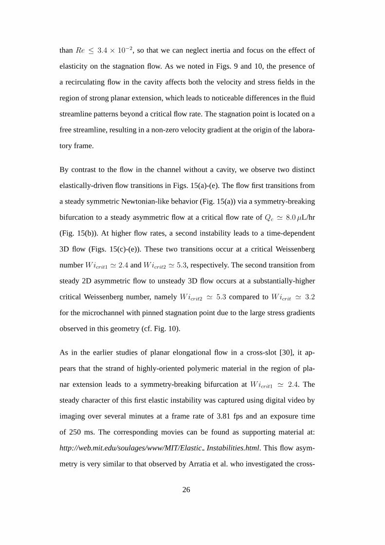
thanRe ≤ 3.4 × 10−2, so that we can neglect inertia and focus on the effect of

elasticity on the stagnation flow. As we noted in Figs. 9 and 10, the presence of

a recirculating flow in the cavity affects both the velocity and stress fields in the

region of strong planar extension, which leads to noticeable differences in the fluid

streamline patterns beyond a critical flow rate. The stagnation point is located on a

free streamline, resulting in a non-zero velocity gradientat the origin of the labora-

tory frame.

By contrast to the flow in the channel without a cavity, we observe two distinct

elastically-driven flow transitions in Figs. 15(a)-(e). The flow first transitions from

a steady symmetric Newtonian-like behavior (Fig. 15(a)) via a symmetry-breaking

bifurcation to a steady asymmetric flow at a critical flow rateof Qc ≃ 8.0 µL/hr

(Fig. 15(b)). At higher flow rates, a second instability leads to a time-dependent

3D flow (Figs. 15(c)-(e)). These two transitions occur at a critical Weissenberg

numberWicrit1 ≃ 2.4 andWicrit2 ≃ 5.3, respectively. The second transition from

steady 2D asymmetric flow to unsteady 3D flow occurs at a substantially-higher

critical Weissenberg number, namelyWicrit2 ≃ 5.3 compared toWicrit ≃ 3.2

for the microchannel with pinned stagnation point due to thelarge stress gradients

observed in this geometry (cf. Fig. 10).

As in the earlier studies of planar elongational flow in a cross-slot [30], it ap-

pears that the strand of highly-oriented polymeric material in the region of pla-

nar extension leads to a symmetry-breaking bifurcation atWicrit1 ≃ 2.4. The

steady character of this first elastic instability was captured using digital video by

imaging over several minutes at a frame rate of 3.81 fps and anexposure time

of 250 ms. The corresponding movies can be found as supporting material at:

http://web.mit.edu/soulages/www/MIT/ElasticInstabilities.html. This flow asym-

metry is very similar to that observed by Arratia et al. who investigated the cross-

26

slot flow of a polyacrylamide viscoelastic solution [30]. Intheir study, the free stag-

nation point coupled to large tensile stresses led to a steady symmetry-breaking

flow asymmetry forWi ≃ 4.5 andRe ≤ 10−2. The asymmetric flow shown in

Fig. 15(b) is also bistable [28, 30] and the mirror image of the recirculating flow

patterns can also be shown experimentally. Small random perturbations in the flow

rate when approaching the critical Weissenberg numberWicrit1 control the final

direction of the flow in the cavity.

At higher flow rates corresponding toWicrit2 ≃ 5.3, the flow transitions from a

steady asymmetric bifurcation to a 3D time-dependent flow asshown in Figs. 15(c)-

(e). The 3D nature of the flow instability is again revealed bythe crossing of the

streaklines. As observed in the geometry without a cavity, the flow eventually be-

comes chaotic at high Weissenberg number, which is desirable for mixing purposes

[65].

The corresponding Newtonian case shown in Figs. 15(f)-(j) is symmetric and stable

for all the volumetric flow rates tested in this study (Re ≤ 6.5×10−2). For the high-

est flow rateQ = 100 µL/hr, a slight asymmetry is visible in the streamline pattern

as shown in Fig. 15(j). This is due to small imbalances in the volumetric flow rates

at the two channel inlets. Because of the large pressure gradients existing at high

flow rates, some leakage between the Tygon tubing and the PDMSchannel can oc-

casionally be seen, which is responsible for the very small observed asymmetry at

high flow rates. Numerical simulations confirm the negligible effect of inertia, and

the predicted streamlines are symmetric and qualitativelysimilar to those predicted

at lower flow rates.

In the next section, predictions of the single-mode SPTT model will be compared

to experimental streak-images before and after the onset ofthe first (steady) flow

27

transition observed in the free stagnation point flow (Wicrit1 ≃ 2.4).

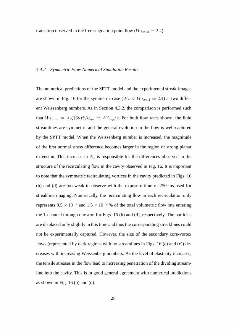
4.4.2 Symmetric Flow Numerical Simulation Results

The numerical predictions of the SPTT model and the experimental streak-images

are shown in Fig. 16 for the symmetric case (Wi < Wicrit1 ≃ 2.4) at two differ-

ent Weissenberg numbers. As in Section 4.3.2, the comparison is performed such

that Winum = λ1ζ(6ν)γ/Uηλ ≃ Wiexp/2. For both flow rates shown, the fluid

streamlines are symmetric and the general evolution in the flow is well-captured

by the SPTT model. When the Weissenberg number is increased,the magnitude

of the first normal stress difference becomes larger in the region of strong planar

extension. This increase inN1 is responsible for the differences observed in the

structure of the recirculating flow in the cavity observed inFig. 16. It is important

to note that the symmetric recirculating vortices in the cavity predicted in Figs. 16

(b) and (d) are too weak to observe with the exposure time of 250 ms used for

streakline imaging. Numerically, the recirculating flow ineach recirculation only

represents 9.5× 10−2 and 1.5× 10−2 % of the total volumetric flow rate entering

the T-channel through one arm for Figs. 16 (b) and (d), respectively. The particles

are displaced only slightly in this time and thus the corresponding streaklines could

not be experimentally captured. However, the size of the secondary core-vortex

flows (represented by dark regions with no streamlines in Figs. 16 (a) and (c)) de-

creases with increasing Weissenberg numbers. As the level of elasticity increases,

the tensile stresses in the flow lead to increasing penetration of the dividing stream-

line into the cavity. This is in good general agreement with numerical predictions

as shown in Fig. 16 (b) and (d).

28

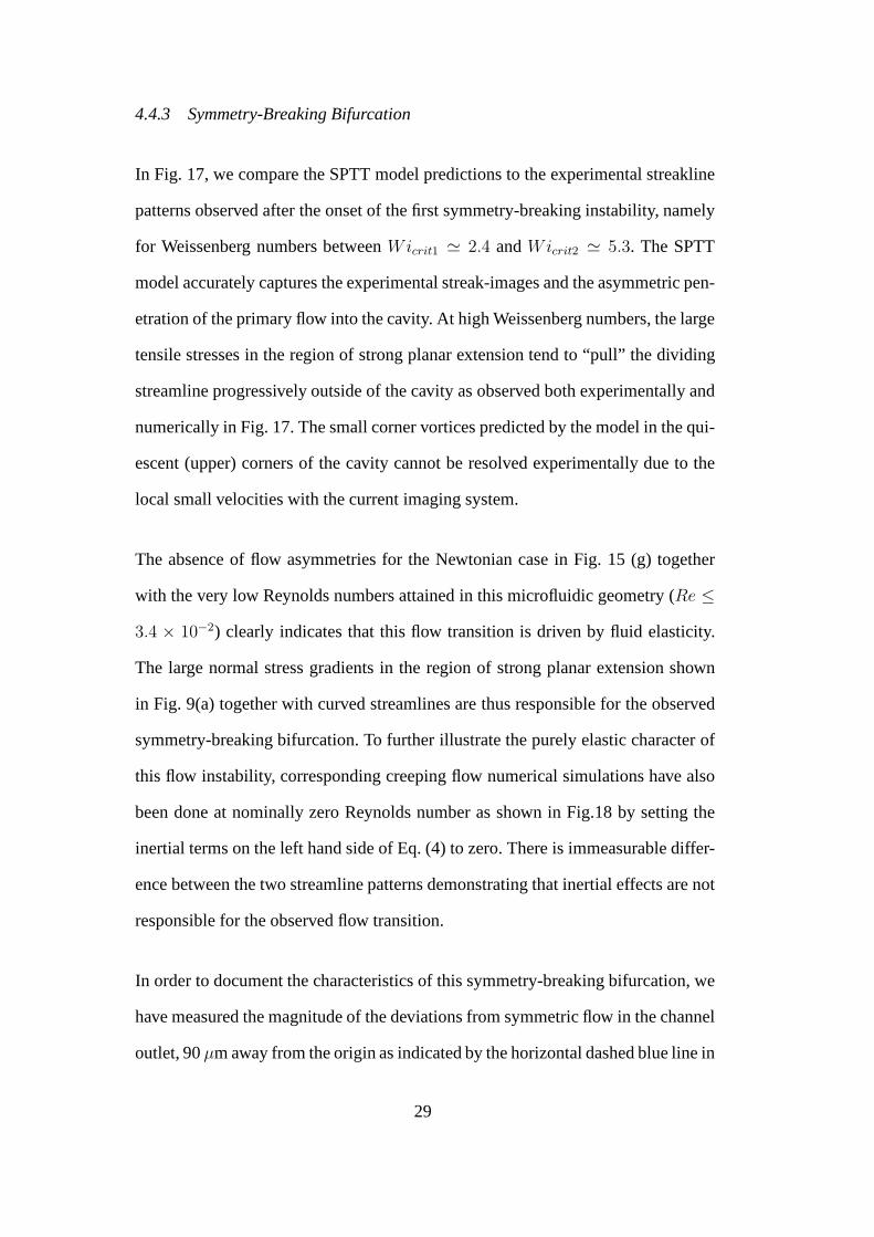
4.4.3 Symmetry-Breaking Bifurcation

In Fig. 17, we compare the SPTT model predictions to the experimental streakline

patterns observed after the onset of the first symmetry-breaking instability, namely

for Weissenberg numbers betweenWicrit1 ≃ 2.4 andWicrit2 ≃ 5.3. The SPTT

model accurately captures the experimental streak-imagesand the asymmetric pen-

etration of the primary flow into the cavity. At high Weissenberg numbers, the large

tensile stresses in the region of strong planar extension tend to “pull” the dividing

streamline progressively outside of the cavity as observedboth experimentally and

numerically in Fig. 17. The small corner vortices predictedby the model in the qui-

escent (upper) corners of the cavity cannot be resolved experimentally due to the

local small velocities with the current imaging system.

The absence of flow asymmetries for the Newtonian case in Fig.15 (g) together

with the very low Reynolds numbers attained in this microfluidic geometry (Re ≤

3.4 × 10−2) clearly indicates that this flow transition is driven by fluid elasticity.

The large normal stress gradients in the region of strong planar extension shown

in Fig. 9(a) together with curved streamlines are thus responsible for the observed

symmetry-breaking bifurcation. To further illustrate thepurely elastic character of

this flow instability, corresponding creeping flow numerical simulations have also

been done at nominally zero Reynolds number as shown in Fig.18 by setting the

inertial terms on the left hand side of Eq. (4) to zero. There is immeasurable differ-

ence between the two streamline patterns demonstrating that inertial effects are not

responsible for the observed flow transition.

In order to document the characteristics of this symmetry-breaking bifurcation, we

have measured the magnitude of the deviations from symmetric flow in the channel

outlet, 90µm away from the origin as indicated by the horizontal dashed blue line in

29

Fig. 19(a). For illustrative purposes, the dividing streamline has also been colored

in black in the figure. Because of mass conservation, for eachincoming stream

entering the microchannel at a volumetric flow rateQ, the volumetric flow rate at

the channel outlet is

Q = V1h1d = V2h2d, (6)

whered represents the (constant) microchannel depth,Vi is the average velocity

for streami (i=1 or 2) andhi is the distance between the dividing streamline and

the microchannel sidewalls measured along thex-axis as shown in Fig. 19(a) (h =

h1 +h2, whereh is the total width of the outflow channel). The squared normalized

velocity deviations from symmetric flow(

∆VV

)2

can thus be written as

(

∆V

V

)2

=

(

V2 − V1

V1

)2

=

(

h1

h2

− 1

)2

. (7)

According to Eq. (7),(

∆VV

)2

= 0 for a symmetric flow and(

∆VV

)2

→ 1 for a

fully asymmetric flow. Figure 19(b) shows the squared normalized velocity de-

viations from symmetric flow as a function of the Weissenbergnumber together

with numerical predictions at a distance of 50, 75 and 90µm away from the origin

of the laboratory frame. The comparison is performed again such thatWinum =

λ1ζ(6ν)γ/ζ(3ν) ≃ Wiexp/2. The results are shown forWi ≤ Wicrit2 and the

maximum Weissenberg number for which convergent numericalresults could be

obtained isWimax = 4.4.

For Wi < Wicrit1, the flow remains symmetric and(

∆VV

)2

≈ 0 (within exper-

imental fluctuations). After the onset of the symmetry-breaking bifurcation, the

magnitude of the asymmetry(

∆VV

)2

varies approximately linearly withWi, a typi-

cal behavior of supercritical bifurcations [72]. The 2D computations underestimate

30

the magnitude of the deviations when the location of the transverse line is taken as

y = 90 µm or y = 75 µm. Much better agreement is found at a distance of 50µm

from the origin of the laboratory frame.

This discrepancy in the strength of the flow asymmetry at a given value ofWi −

Wicrit1 > 0 may be a consequence of the finite depth of the T-channel geometry

(d = 50 µm) which gives rise to three-dimensionality in the local experimental flow

that cannot be captured by the 2D simulations.

The observations and calculations strongly suggest that the observed bifurcation

is a supercritical steady viscoelastic flow transition withstrong similarities to the

cross-slot observations of Arratia et al. [30] that were duplicated numerically by

Poole and coworkers [35].

5 Conclusion and Outlook

In this study, we have investigated the structure and stability of steady planar stag-

nation flows of a dilute viscoelastic PEO solution using two different T-shaped mi-

crochannels, with and without, a recirculating cavity region, respectively. We have

shown that the kinematic differences near the stagnation point in these two geome-

tries control the magnitude of the large tensile normal stress differences in the vicin-

ity of the stagnation point as well as the critical conditions and spatiotemporal dy-

namics of the resulting elastically-driven flow asymmetries. For the free stagnation

point flow, a strand of highly-oriented polymeric material is formed in the region of

strong planar extensional flow, which results in an additional symmetry-breaking

transition at intermediate Weissenberg numbers. For each stagnation flow, we also

observed a flow transition from a steady to a three-dimensional time-dependent

31

flow at a critical Weissenberg number. The critical conditions are substantially-

lower for the pinned stagnation point flow.

The spatial characteristics of these purely elastic flow instabilities were compared

with two-dimensional numerical predictions using a single-mode simplified Phan-

Thien-Tanner (SPTT) model. The calculations were shown to quantitatively capture

the evolution in the streamline patterns with increasing Weissenberg number as well

as predict the onset of a steady 2D asymmetric flow beyond a critical flow rate.

Idealized creeping flow calculations with no fluid inertia demonstrate the purely

elastic nature of the different flow transitions.

Future work will involve a detailed analysis of the local velocity field in the vicinity

of the stagnation point using microparticle image velocimetry to further document

the nature of the bifurcation. We also hope to make use of other viscoelastic flu-

ids such as wormlike micellar solutions to investigate the role of the magnitude of

strain-hardening in the extensional viscosity on the localstresses near the stagna-

tion point and the corresponding flow stability.

6 Acknowledgments

This work made use of facilities in the MIT MicroelectronicsTechnology Labora-

tory and was supported by the Swiss National Science Foundation (Grant PBEZ2-

115179). The authors acknowledge the funding support provided by Fundacao

para a Ciencia e a Tecnologia under projects PTDC/EQU-FTT/71800/2006 and

PTDC/EQU-FTT/70727/2006.

32

References

[1] H. A. Stone and S. Kim. Microfluidics: basic issues, applications, and chal-

lenges.AIChE Journal, 47(6):1250–1254, 2001.

[2] G. M. Whitesides. The origins and the future of microfluidics. Nature,

442(7101):368–373, 2006.

[3] P. Gravesen, J. Branebjerg, and O. S. Jensen. Microfluidics - A review.Jour-

nal of micromechanics and microengineering, 3:168–182, 1993.

[4] T. Pfohl, F. Mugele, R. Seemann, and S. Herminghaus. Trends in microflu-

idics with complex fluids.ChemPhysChem, 4(12):1291–1298, 2003.

[5] T. M. Squires and S. R. Quake. Microfluidics: fluid physicsat the nanoliter

scale.Reviews of Modern Physics, 77(3):977–1026, 2005.

[6] D. J. Beebe, G. A. Mensing, and G. M. Walker. Physics and applications of

microfluidics in biology.Annual Review of Biomedical Engineering, 4:261–

286, 2002.

[7] C. Hansen and S. R. Quake. Microfluidics in structural biology: smaller,

faster... better.Current Opinion in Structural Biology, 13(5):538–544, 2003.

[8] C. J. Pipe and G. H. McKinley. Microfluidic rheometry.Mech. Research

Comm., 36:110–120, 2009.

[9] P. Pakdel and G. H. McKinley. Elastic instability and curved streamlines.

Physical Review Letters, 77(12):2459–2462, 1996.

[10] A. Oztekin, B. Alakus, and G. H. McKinley. Stability of planar stagnation

flow of a highly viscoelastic fluid.Journal of Non-Newtonian Fluid Mechan-

ics, 72(1):1–29, 1997.

[11] W. B. Zimmerman, J. M. Rees, and T. J. Craven. Rheometry of non-

Newtonian electrokinetic flow in a microchannel T-junction. Microfluid

Nanofluid, 2:481–492, 2006.

33

[12] K. Walters and R. I. Tanner.The Motion of a Sphere Through an Elastic

Liquid. Transport Processes in Bubbles, Drops and Particles, p. 73-86, R. P.

Chhabra and D. De Kee (ed.), Hemisphere Publ. Corp., New York, 1992.

[13] G. H. McKinley. Steady and Transient Motion of Spherical Particles in Vis-

coelastic Liquids. Transport Processes in Bubbles, Drops and Particles, Chap-

ter 14, p. 338-375, R. P. Chhabra and D. De Kee (ed.), Taylor and Francis,

New York, 2002.

[14] C. Bisgaard. Velocity fields around spheres and bubblesinvestigated by

Laser-Doppler Anemometry.Journal of Non-Newtonian Fluid Mechanics,

12(3):283–302, 1983.

[15] R. You, A. Borhan, and H. Haj-Hariri. A finite volume formulation for sim-

ulating drop motion in a viscoelastic two-phase system.Journal of Non-

Newtonian Fluid Mechanics, 153(2-3):109–129, 2008.

[16] F. Pan and A. Acrivos. Steady flows in rectangular cavities.Journal of Fluid

Mechanics, 28:643, 1967.

[17] S. Taneda. Visualization of separating Stokes flows.Journal of the Physical

Society of Japan, 46(6):1935–1942, 1979.

[18] M. G. N. Perera and K. Walters. Long-range memory effects in flows involv-

ing abrupt changes in geometry; Part I: Flows associated with L-shaped and

T-shaped geometries.Journal of Non-Newtonian Fluid Mechanics, 2(1):49–

81, 1977.

[19] T. Nishimura, K. Nakamura, and A. Horikawa. Two-dimensional viscoelastic

flow of polymer solution at channel junction and branch; Part1: T-shaped

junction flow. Journal of the Textile Machinery Society of Japan, 31(1):1–6,

1985.

[20] D. M. Binding, K. Walters, J. Dheur, and M. J. Crochet. Interfacial effects in

the flow of viscous and elastoviscous liquids.Philosophical Transactions of

34

the Royal Society of London Series A-Mathematical Physicaland Engineering

Sciences, 323(1573):449, 1987.

[21] L. E. Rodd, T. P. Scott, D. V. Boger, J. J. Cooper-White, and G. H. McKin-

ley. The inertio-elastic planar entry flow of low-viscosityelastic fluids in

micro-fabricated geometries.Journal of Non-Newtonian Fluid Mechanics,

129(1):1–22, 2005.

[22] L. E. Rodd, J. J. Cooper-White, D. V. Boger, and G. H. McKinley. Role of

the elasticity number in the entry flow of dilute polymer solutions in micro-

fabricated contraction geometries.Journal of Non-Newtonian Fluid Mechan-

ics, 143(2-3):170–191, 2007.

[23] E. S. G. Shaqfeh, S. J. Muller, and R. G. Larson. The effects of gap width

and dilute-solution properties on the viscoelastic TaylorCouette instability.

Journal of Fluid Mechanics, 235:285–317, 1992.

[24] G. H. McKinley, P. Pakdel, and A. Oztekin. Rheological and geometric scal-

ing of purely elastic flow instabilities.Journal of Non-Newtonian Fluid Me-

chanics, 67:19–47, 1996.

[25] A. Groisman and V. Steinberg. Efficient mixing at low Reynolds numbers

using polymer additives.Nature, 410(6831):905–908, 2001.

[26] S. Gulati, D. Liepmann, and S. J. Muller. Elastic secondary flows of

semidilute DNA solutions in abrupt 90 microbends. Physical Review E,

78(3):036314, 2008.

[27] S. Gulati, S. J. Muller, and D. Liepmann. Direct measurements of viscoelas-

tic flows of DNA in a 2:1 abrupt planar micro-contraction.Journal of Non-

Newtonian Fluid Mechanics, 155(1-2):51–66, 2008.

[28] A. Groisman, M. Enzelberger, and S. R. Quake. Microfluidic memory and

control devices.Science, 300(5621):955–958, 2003.

[29] A. Groisman and S. R. Quake. A microfluidic rectifier: anisotropic flow re-

35

sistance at low reynolds numbers.Physical Review Letters, 92(9):094501–1–

094501–4, 2004.

[30] P. E. Arratia, C. C. Thomas, J. Diorio, and J. P. Gollub. Elastic instabil-

ities of polymer solutions in cross-channel flow.Physical Review Letters,

96(14):144502, 2006.

[31] E. F. Humphrey and D. H. Tarumoto.Fluidics. Fluid Amplifier Associates,

Boston, 1965.

[32] K. Foster and G. A. Parker.Fluidics: components and circuits. Wiley Inter-

science, London, 1970.

[33] J. A. Odell and S. P. Carrington.Polymer Solutions in Strong Stagnation Point

Extensional Flows. Flexible Polymer Chains in Elongational Flow: Theory

and Experiment, Springer-Verlag, Berlin, 1999.

[34] J. A. Pathak and S. D. Hudson. Rheo-optics of equilibrium polymer solutions:

Wormlike micelles in elongational flow in a microfluidic cross-slot. Macro-

molecules, 39(25):8782–8792, 2006.

[35] R. J. Poole, M. A. Alves, and P. J. Oliveira. Purely elastic flow asymmetries.

Physical Review Letters, 99(16):164503, 2007.

[36] N.-T. Nguyen and S. T Wereley.Fundamentals and Applications of Microflu-

idics. Artech House, 2002.

[37] D. C. Duffy, J. C. McDonald, O. J. A. Schueller, and G. M. Whitesides. Rapid

prototyping of microfluidic systems in poly(dimethylsiloxane). Analytical

Chemistry, 70(23):4974–4984, 1998.

[38] Y. N. Xia and G. M. Whitesides. Soft lithography.Annual Review of Materials

Science, 28:153–184, 1998.

[39] J. C. McDonald, D. C. Duffy, J. R. Anderson, D. T. Chiu, H.K. Wu, O. J. A.

Schueller, and G. M. Whitesides. Fabrication of microfluidic systems in

poly(dimethylsiloxane).Electrophoresis, 21(1):27–40, 2000.

36

[40] J. M. K. Ng, I. Gitlin, A. D. Stroock, and G. M. Whitesides. Components

for integrated poly(dimethylsiloxane) microfluidic systems. Electrophoresis,

23(20):3461–3473, 2002.

[41] T. P. Scott. Contraction/Expansion Flow of Dilute Elastic Solutions in Mi-

crochannels. M. S. Thesis, MIT, 2004.

[42] R. G. Larson. Instabilities in viscoelastic flows.Rheologica Acta, 31(3):213–

263, 1992.

[43] G. H. McKinley and A. Tripathi. How to extract the Newtonian viscosity

from capillary breakup measurements in a filament rheometer. Journal of

Rheology, 44(3):653–670, 2000.

[44] S. L. Anna and G. H. McKinley. Elasto-capillary thinning and breakup of

model elastic liquids.Journal of Rheology, 45(1):115–138, 2001.

[45] L. E. Rodd, T. P. Scott, J. J. Cooper-White, and G. H. McKinley. Capil-

lary break-up rheometry of low-viscosity elastic fluids.Applied Rheology,

15(1):12–27, 2005.

[46] N. Phan-Thien and R. I. Tanner. New constitutive equation derived from

network theory.Journal of Non-Newtonian Fluid Mechanics, 2(4):353–365,

1977.

[47] C. Clasen, J. P. Plog, W. M. Kulicke, M. Owens, C. Macosko, L. E. Scriven,

M. Verani, and G. H. McKinley. How dilute are dilute solutions in extensional

flows?Journal of Rheology, 50(6):849–881, 2006.

[48] V. Tirtaatmadja, G. H. McKinley, and J. J. Cooper-White. Drop formation

and breakup of low viscosity elastic fluids: Effects of molecular weight and

concentration.Physics of Fluids, 18(4):043101, 2006.

[49] W. W. Graessley. Polymer chain dimensions and the dependence of viscoelas-

tic properties on concentration, molecular weight and solvent power.Polymer,

21(3):258–262, 1980.

37

[50] M. S. N. Oliveira, M. A. Alves, F. T. Pinho, and G. H. McKinley. Viscous

flow through microfabricated hyperbolic contractions.Experiments in Fluids,

43(2-3):437–451, 2007.

[51] P. J. Oliveira, F. T. Pinho, and G. A. Pinto. Numerical simulation of non-

linear elastic flows with a general collocated finite-volumemethod.Journal

of Non-Newtonian Fluid Mechanics, 79(1):1–43, 1998.

[52] P. J. Oliveira and F. T. Pinho. Numerical procedure for the computation of

fluid flow with arbitrary stress-strain relationships.Numerical Heat Transfer

Part B-Fundamentals, 35(3):295–315, 1999.

[53] M. A. Alves, P. J. Oliveira, and F. T. Pinho. Benchmark solutions for the

flow of Oldroyd-B and PTT fluids in planar contractions.Journal of Non-

Newtonian Fluid Mechanics, 110(1):45–75, 2003.

[54] P. J. Oliveira and F. T. Pinho. Plane contraction flows ofupper convected

Maxwell and Phan-Thien–Tanner fluids as predicted by a finite-volume

method.Journal of Non-Newtonian Fluid Mechanics, 88(1-2):63–88, 1999.

[55] M. S. N. Oliveira, P. J. Oliveira, F. T. Pinho, and M. A. Alves. Effect of

contraction ratio upon viscoelastic flow in contractions: The axisymmetric

case.Journal of Non-Newtonian Fluid Mechanics, 147(1-2):92–108, 2007.

[56] M. S. N. Oliveira, L. E. Rodd, G. H. McKinley, and M. A. Alves. Simulations

of extensional flow in microrheometric devices.Microfluidics Nanofluidics,

5:809–826, 2008.

[57] M. A. Alves, P. J. Oliveira, and F. T. Pinho. A convergentand universally

bounded interpolation scheme for the treatment of advection. International

Journal for Numerical Methods in Fluids, 41(1):47–75, 2003.

[58] R. G. Larson.Constitutive Equations for Polymer Melts and Solutions. But-

terworth Publishers, 1988.

[59] R. Fattal and R. Kupferman. Constitutive laws for the matrix-logarithm of

38

the conformation tensor.Journal of Non-Newtonian Fluid Mechanics, 123(2-

3):281–285, 2004.

[60] A. M. Afonso, P. J. Oliveira, F. T. Pinho, and M. A. Alves.The log confor-

mation tensor approach in the finite volume method framework. Journal of

Non-Newtonian Fluid Mechanics, 157(1-2):55–65, 2009.

[61] O. G. Harlen. High-Deborah-number flow of a dilute polymer solution past a

sphere falling along the axis of a cylindrical tube.Journal of Non-Newtonian

Fluid Mechanics, 37(2-3), 1990.

[62] M. A. Alves, F. T. Pinho, and P. J. Oliveira. The flow of viscoelastic fluids past

a cylinder: finite-volume high-resolution methods.Journal of Non-Newtonian

Fluid Mechanics, 97(2-3):207–232, 2001.

[63] M. A. Hulsen, R. Fattal, and R. Kupferman. Flow of viscoelastic fluids past

a cylinder at high Weissenberg number: Stabilized simulations using matrix

logarithms.Journal of Non-Newtonian Fluid Mechanics, 127(1):27–39, 2005.

[64] G. H. McKinley, R. C. Armstrong, and R. A. Brown. The wakeinstability

in viscoelastic flow past confined circular-cylinders.Philosophical Trans-

actions of the Royal Society of London Series A-Mathematical Physical and

Engineering Sciences, 344(1671):265–304, 1993.

[65] J. M. Ottino and S. Wiggins. Applied physics - Designingoptimal micromix-

ers.Science, 305(5683):485–486, 2004.

[66] P. Becherer, W. Saarloos, and A. N. Morozov. Stress singularities and the for-

mation of birefringent strands in stagnation flows of dilutepolymer solutions.

Journal of Non-Newtonian Fluid Mechanics, 157(1-2):126–132, 2009.

[67] H. C.Ottinger.Stochastic Processes in Polymeric Fluids: Tools and Examples

for Developing Simulation Algorithms. Springer-Verlag, Berlin, 1996.

[68] M. Kroger, A. Alba-Perez, M. Laso, and H. C.Ottinger. Variance reduced

brownian simulation of a bead-spring chain under steady shear flow con-

39

sidering hydrodynamic interaction effects.Journal of Chemical Physics,

113(11):4767–4773, 2000.

[69] V. M. Entov and E. J. Hinch. Effect of a spectrum of relaxation times on the

capillary thinning of a filament of elastic liquid.Journal of Non-Newtonian

Fluid Mechanics, 72(1):31–53, 1997.

[70] J. P. Rothstein and G. H. McKinley. Non-isothermal modification of purely

elastic flow instabilities in torsional flows of polymeric fluids. Physics of

Fluids, 13(2):382–396, 2001.

[71] I. Ghosh, G. H. McKinley, Robert A. Brown, and R. C. Armstrong. Deficien-

cies of FENE dumbbell models in describing the rapid stretching of dilute

polymer solutions.Journal of Rheology, 45(3):721–758, 2001.

[72] G. Iooss and D. Joseph.Elementary Stability and Bifurcation Theory.

Springer-Verlag, Berlin, 1980.

40

Table 1

Working fluid rheological properties at 23C.

Zero-shear rate viscosity η0 [mPa s] 19.5

Solvent viscosity ηS [mPa s] 9.8

Polymer viscosity ηP [mPa s] 9.7

Zimm relaxation time λZimm [ms] 2.3

CaBER relaxation time λCaBER [ms] 66

Intrinsic viscosity [η] [mL/g] 582

Density ρ [kg/m3] 1196

Polymer concentration c [g/mL] 8.97×10−4

Concentration ratio c/c⋆ 0.68

41

(a) Microchannel with cavity.

(b) Microchannel without cavity.

Fig. 1. Streamline predictions for Newtonian flow within a T-shaped microchannel with

and without a recirculating cavity:Q= 6µL/hr; S.P. denotes the location of the stagnation

point (Re = 2.05 × 10−3).

42

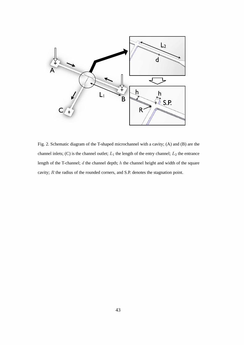
Fig. 2. Schematic diagram of the T-shaped microchannel witha cavity; (A) and (B) are the

channel inlets; (C) is the channel outlet;L1 the length of the entry channel;L2 the entrance

length of the T-channel;d the channel depth;h the channel height and width of the square

cavity; R the radius of the rounded corners, and S.P. denotes the stagnation point.

43

(a) Microchannel with cavity. (b) Microchannel without cavity.

Fig. 3. Optical micrographs of the microchannel (a) with and(b) without cavity (20×, 0.5

N.A.). The in- and outflow directions are indicated by the white arrows. The anticipated

location of the stagnation point (S.P.) sitting on a free streamline (a) or pinned onto the

confining wall (b) is indicated in the channel.

(a) (b)

Fig. 4. Microchannel SEM image (a) and optical micrograph ofthe channel cross-section

(b) showing the well-defined geometries achievable with soft lithography.

44

100 101 102 103 10410-3

10-2

10-1

(ii)

(i)

1 PEO solution Solvent (glycerol/water) solution Oldroyd-B Model ( = 0) SPTT Model ( = 7x10-6)19.5 mPas

[Pas

]

Shear rate [s-1]

9.8 mPas

CaBER

Fig. 5. Steady shear data measured at 23C in a double gap Couette geometry using a con-

trolled stress rheometer (AR-G2, TA Instruments). In the case of the PEO solution, the open

symbols represent repeated experiments. The SPTT model predictions are shown by the red

dashed and solid lines forε = 0 (Oldroyd-B model) andε = 7.0 × 10−6, respectively. (i):

minimum measurable shear viscosity based on 20 times the minimum torque resolvable by

the rheometer (2 × 10−6Nm); (ii): maximum measurable shear viscosity before the onset

of Taylor instabilities;λCaBER: relaxation time determined from CaBER measurements as

shown in Fig. 6.

45

0.0 0.2 0.4 0.6 0.8 1.010-4

10-3

10-2

10-1

100

3 = 1x10-6

= 4x10-6

= 7x10-6

Experiment 1 Experiment 2 Oldroyd-B SPTT

R/R

0 [-]

t [s]

Minimum resolvable radius

-1

Increasing

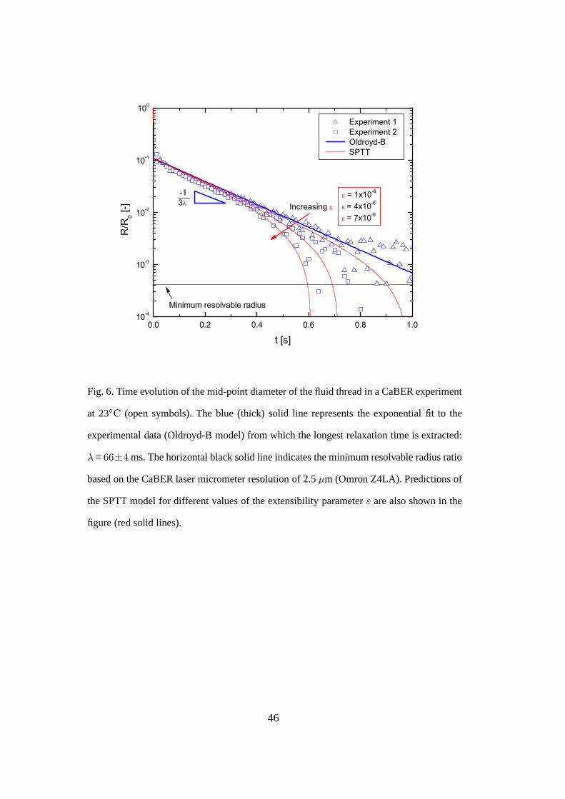
Fig. 6. Time evolution of the mid-point diameter of the fluid thread in a CaBER experiment

at 23C (open symbols). The blue (thick) solid line represents the exponential fit to the

experimental data (Oldroyd-B model) from which the longestrelaxation time is extracted:

λ = 66±4 ms. The horizontal black solid line indicates the minimum resolvable radius ratio

based on the CaBER laser micrometer resolution of 2.5µm (Omron Z4LA). Predictions of

the SPTT model for different values of the extensibility parameterε are also shown in the

figure (red solid lines).

46

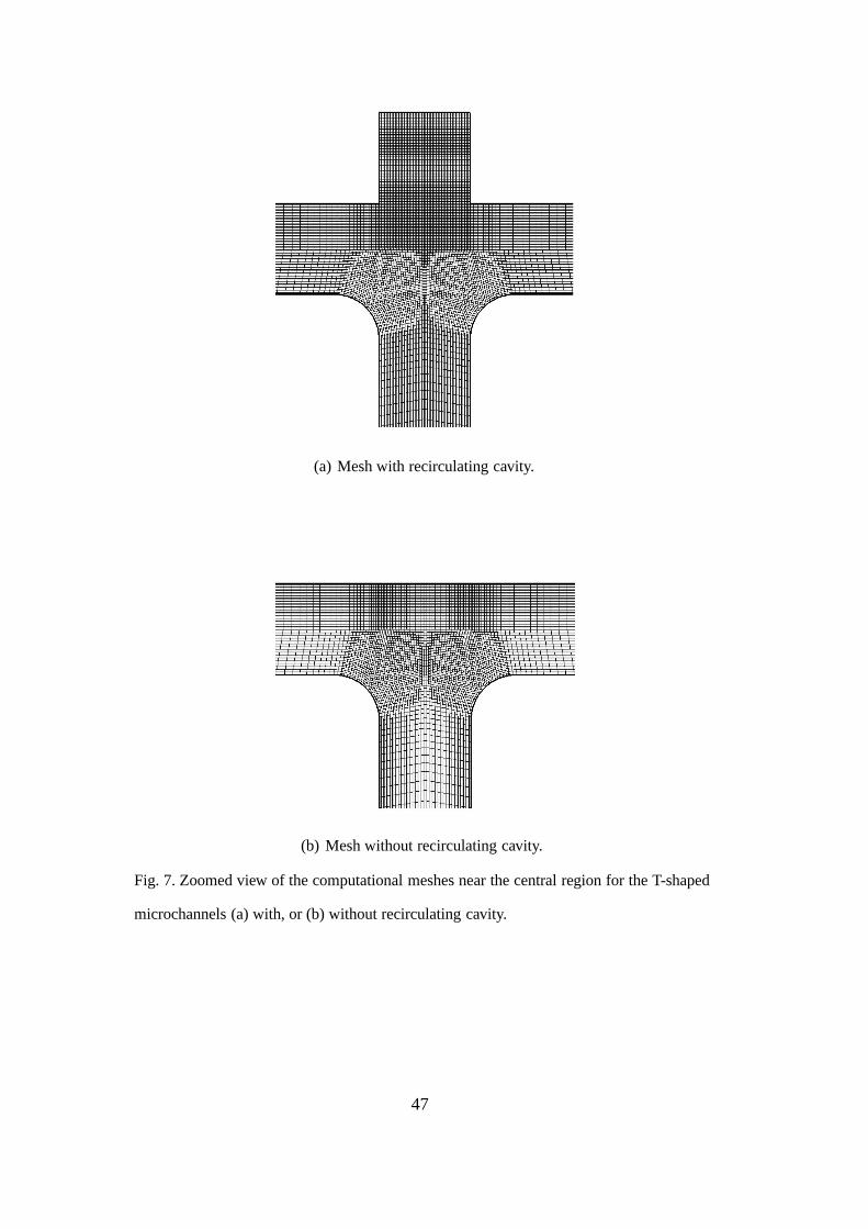
(a) Mesh with recirculating cavity.

(b) Mesh without recirculating cavity.

Fig. 7. Zoomed view of the computational meshes near the central region for the T-shaped

microchannels (a) with, or (b) without recirculating cavity.

47

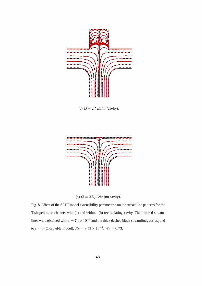
(a) Q = 2.5µL/hr (cavity).

(b) Q = 2.5µL/hr (no cavity).

Fig. 8. Effect of the SPTT model extensibility parameterε on the streamline patterns for the

T-shaped microchannel with (a) and without (b) recirculating cavity. The thin red stream-

lines were obtained withε = 7.0×10−6 and the thick dashed black streamlines correspond

to ε = 0 (Oldroyd-B model);Re = 8.53 × 10−4, Wi = 0.73.

48

(a) Q = 2.5µL/hr (cavity).

(b) Q = 2.5µL/hr (no cavity).

Fig. 9. Contour plots of the normalized first normal stress difference (h(τyy−τxx)/(2η0V ))

for the T-shaped microchannel without (a), and with (b), recirculating cavity (SPTT model;

β = 0.50, ε = 7.0 × 10−6, Re = 8.53 × 10−4, Wi = 0.73).

49

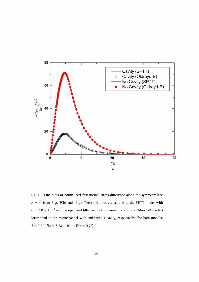
Fig. 10. Line plots of normalized first normal stress difference along the symmetry line

x = 0 from Figs. 9(b) and 9(a). The solid lines correspond to the SPTT model with

ε = 7.0 × 10−6 and the open and filled symbols obtained forε = 0 (Oldroyd-B model)

correspond to the microchannel with and without cavity, respectively (for both models:

β = 0.50, Re = 8.53 × 10−4, Wi = 0.73).

50

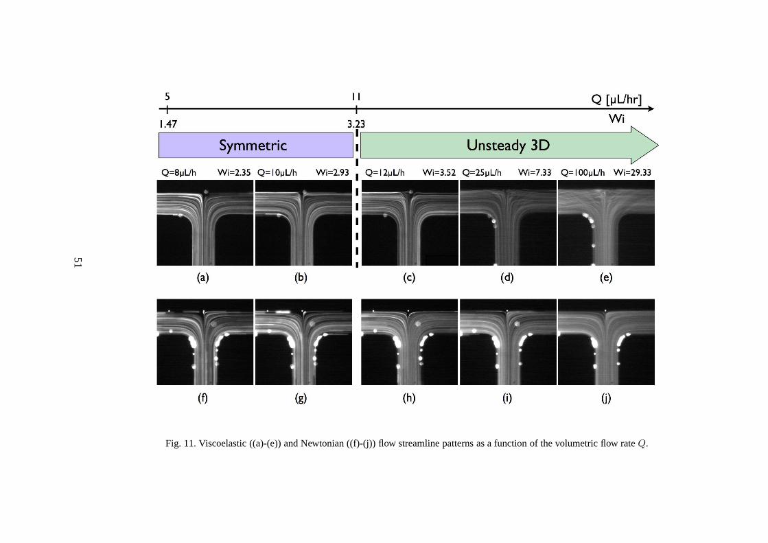
Fig. 11. Viscoelastic ((a)-(e)) and Newtonian ((f)-(j)) flow streamline patterns as a function of the volumetric flow rateQ.

51

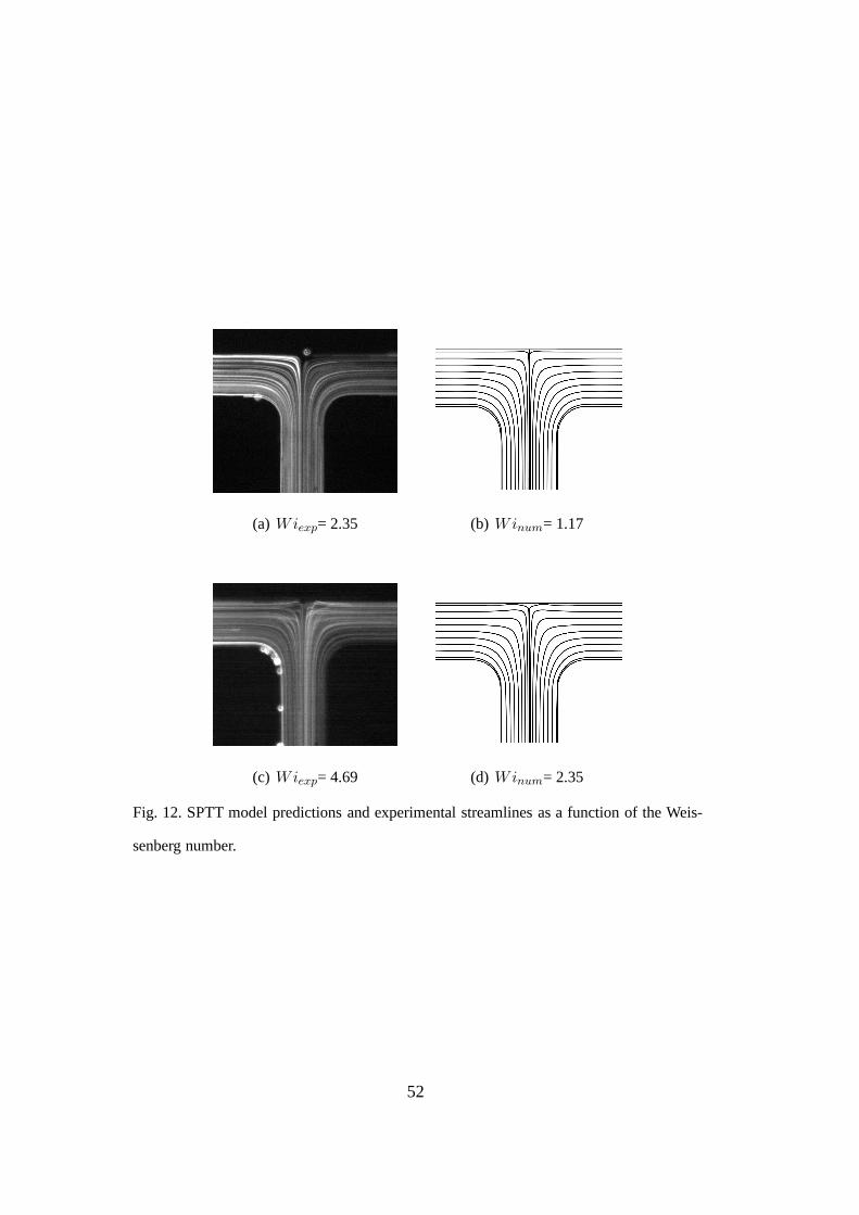
(a) Wiexp= 2.35 (b) Winum= 1.17

(c) Wiexp= 4.69 (d) Winum= 2.35

Fig. 12. SPTT model predictions and experimental streamlines as a function of the Weis-

senberg number.

52

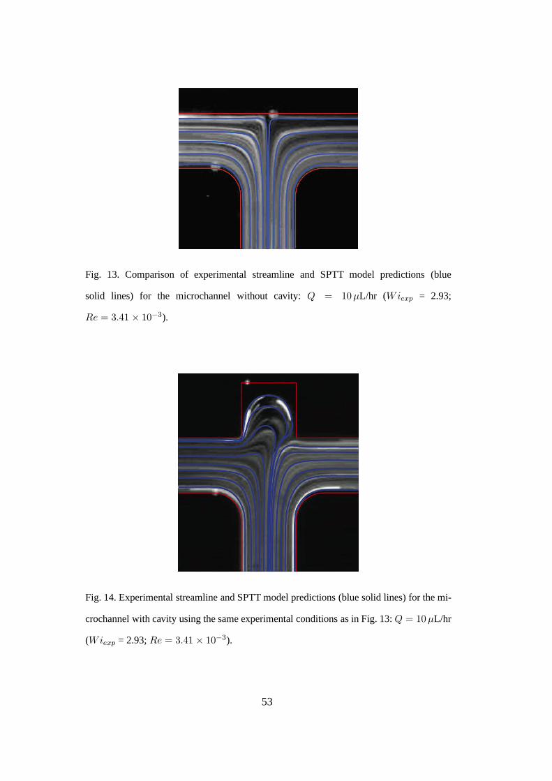
Fig. 13. Comparison of experimental streamline and SPTT model predictions (blue

solid lines) for the microchannel without cavity:Q = 10µL/hr (Wiexp = 2.93;

Re = 3.41 × 10−3).

Fig. 14. Experimental streamline and SPTT model predictions (blue solid lines) for the mi-

crochannel with cavity using the same experimental conditions as in Fig. 13:Q = 10µL/hr

(Wiexp = 2.93;Re = 3.41 × 10−3).

53

Fig. 15. Viscoelastic ((a)-(e)) and Newtonian ((f)-(j)) flow streamline patterns as a function of the volumetric flow rateQ.

54

(a) Wiexp= 1.17 (b) Winum= 0.59

(c) Wiexp= 2.05 (d) Winum= 1.17

Fig. 16. SPTT model predictions ((b) and (d)) for the viscoelastic evolution in the steady

streamlines and experimental streaklines ((a) and (c)) forsymmetric flow as the flow rate is

increased.

55

(a) Wiexp= 2.64 (b) Winum= 1.32

(c) Wiexp= 3.52 (d) Winum= 1.76

Fig. 17. SPTT model predictions ((b) and (d)) for the viscoelastic evolution in the steady

streamlines and experimental streaklines ((a) and (c)) forsteady asymmetric flow as the

flow rate is increased.

56

Fig. 18. Effect of inertia on the streamline patterns for theT-shaped microchannel with re-

circulating cavity (ε = 7.0×10−6). The solid red and dashed black streamlines correspond

to finite inertia (Re = 2.05×10−3) and creeping (Re = 0) flow, respectively (Wi = 1.76).

57

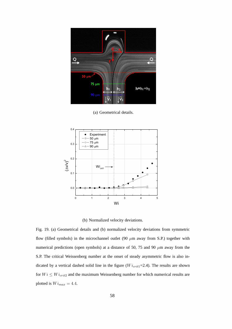
(a) Geometrical details.

0 1 2 3 4 5

0.0

0.1

0.2

0.3

0.4

Experiment 50 m 75 m 90 m

(v/

v)2

Wi

Wicrit1

(b) Normalized velocity deviations.

Fig. 19. (a) Geometrical details and (b) normalized velocity deviations from symmetric

flow (filled symbols) in the microchannel outlet (90µm away from S.P.) together with

numerical predictions (open symbols) at a distance of 50, 75and 90µm away from the

S.P. The critical Weissenberg number at the onset of steady asymmetric flow is also in-

dicated by a vertical dashed solid line in the figure (Wicrit1=2.4). The results are shown

for Wi ≤ Wicrit2 and the maximum Weissenberg number for which numerical results are

plotted isWimax = 4.4.

58