investigating the domain of geometric inductive reasoning
TRANSCRIPT

Brigham Young University Brigham Young University
BYU ScholarsArchive BYU ScholarsArchive
Theses and Dissertations
2008-04-26
Investigating the Domain of Geometric Inductive Reasoning Investigating the Domain of Geometric Inductive Reasoning
Problems: A Structural Equation Modeling Analysis Problems: A Structural Equation Modeling Analysis
Kairong Wang Brigham Young University - Provo
Follow this and additional works at: https://scholarsarchive.byu.edu/etd
Part of the Educational Psychology Commons
BYU ScholarsArchive Citation BYU ScholarsArchive Citation Wang, Kairong, "Investigating the Domain of Geometric Inductive Reasoning Problems: A Structural Equation Modeling Analysis" (2008). Theses and Dissertations. 1420. https://scholarsarchive.byu.edu/etd/1420
This Dissertation is brought to you for free and open access by BYU ScholarsArchive. It has been accepted for inclusion in Theses and Dissertations by an authorized administrator of BYU ScholarsArchive. For more information, please contact [email protected], [email protected].

INVESTIGATING THE DOMAIN OF GEOMETRIC INDUCTIVE REASONING
PROBLEMS: A STRUCTURAL EQUATION MODELING ANALYSIS
by
Kairong Wang
A dissertation submitted to the faculty of
Brigham Young University
in partial fulfillment of the requirements for the degree of
Doctor of Philosophy
Department of Instructional Psychology and Technology
Brigham Young University
April 2008

Copyright © 2008 Kairong Wang
All Rights Reserved

BRIGHAM YOUNG UNIVERSITY
GRADUATE COMMITTEE APPROVAL
of a dissertation submitted by
Kairong Wang
This dissertation has been read by each member of the following graduate committee and by majority vote has been found to be satisfactory.
Date Richard R Sudweeks, Chair
Date C. Victor Bunderson
Date Andrew S. Gibbons
Date Paul F. Merrill
Date Joseph A. Olsen

BRIGHAM YOUNG UNIVERSITY
As chair of the candidate’s graduate committee, I have read the dissertation of Kairong Wang in its final form and have found that (1) its format, citations, and bibliographical style are consistent and acceptable and fulfill university and department style requirements; (2) its illustrative materials including figures, tables, and charts are in place; and (3) the final manuscript is satisfactory to the graduate committee and is ready for submission to the university library. Date Richard R Sudweeeks Chair, Graduate Committee Accepted for the Department Andrew S. Gibbons Department Chair Accepted for the School K. Richard Young Dean, David O. McKay School of
Education

ABSTRACT
INVESTIGATING THE DOMAIN OF GEOMETRIC INDUCTIVE REASONING
PROBLEMS: A STRUCTURAL EQUATION MODELING ANALYSIS
Kairong Wang
Department of Instructional Psychology and Technology
Doctor of Philosophy
Matrix inductive reasoning has been a popular research topic due to its claimed
relationship with the general factor of intelligence. In this research, four subabilities were
identified: working memory, rule induction, rule application, and figure detection. This
quantitative study examined the relationship between these four subabilites and students’
general ability to solve Matrix Reasoning problems. Using tests developed for this
research to measure the identified subabilities, the data were collected from 334 Chinese
students aged from 12 to 15. Structural equation modeling method was used to analyze
the collected data and to evaluate the hypothesized models.
Results from the analysis showed that a valid model existed to represent the
construct of matrix inductive reasoning. Except for figural detection ability, the other
three subabilities had significant direct effects on matrix inductive reasoning ability.
Readers should interpret from this result with caution due to the unsatisfactory reliability
of the Figure Detection scores.

To improve the validity of the interpretation, a new model without the latent
variable of figure detection was reexamined. In this analysis, significant relationships still
existed from the three subablities to matrix inductive reasoning ability. The strongest
relationship existed from working memory ability to matrix reasoning ability, with a
standardized coefficient of .52. Effects from rule induction and rule application ability to
matrix reasoning dropped to .36 and .34 respectively. These results suggested the
important role of working memory on solving inductive reasoning problems. In addition,
a significant and substantial indirect path was found that lead from working memory
rule induction rule application matrix reasoning. The indirect path indicated that a
process existed when students solved Matrix Reasoning tasks.

ACKNOWLEDGEMENTS
Studying at BYU has been a blessing in my life. I have always been touched by
the love and support surrounding me. There are many who I would like to acknowledge
for helping and encouraging me to complete my studies.
Dr. Richard Sudweeks, my committee chair, has always been supportive of this
research. I appreciate his thoughtful suggestions and editing. I gratefully acknowledge
the many conversations with him and his advice on finishing the dissertation.
I will take this chance to express my special thanks to Dr. Victor Bunderson, from
whom I have been studying since my enrollment in this department. His enthusiasms for
research and wise thoughts have always been inspiring. His kind and spiritual words are
always encouraging.
I would like to sincerely thank Dr. Joseph Olsen from the College of Family,
Home and Social Sciences. His specialized assistance on the structural equation modeling
technique made the completion of this research possible.
I am really grateful to Dr. Paul Merrill and Dr. Andy Gibbons. Dr. Merrill has
provided tremendous help developing the online test to collect data. I learned all my
technical knowledge from him. Dr. Gibbons provided valuable advice about writing the
dissertation, which will be precious for my future career.

Many thanks will also go to Dr. Jiliang Shen from Beijing Normal University.
The data collection would not have been possible without his help. I am so glad I have a
mentor like him.
Last, but not the least, I would like to thank family members. They provided
unbounded support and love to me. They always stood by my side. I could not have gone
this far without their encouragement. I owe a debt of gratitude to my three wonderful
little girls: Anabell, Rebecca and Christina. They are the source of all my joy.

ix
TABLE OF CONTENTS
ABSTRACT...............................................................................................................… …..v ACKNOWLEDGEMENTS.......................................................................................…….vii LIST OF TABLES.....................................................................................................… ….ix LIST OF FIGURES ..................................................................................................… ….xi Chapter 1: Introduction ......................................................................................................... 1
Need for Research on Matrix Inductive Reasoning.......................................................... 1 Background....................................................................................................................... 3 Rationale for This Study ................................................................................................... 5 Purpose and Research Questions ...................................................................................... 7
Chapter 2: Review of the Literature...................................................................................... 8 Issues Pertaining to a Domain Theory .............................................................................. 8 General Introduction to Matrix Inductive Reasoning ....................................................... 9 Item Difficulty Resources of Matrix Inductive Reasoning Problems............................. 11 Constructs of Matrix Inductive Reasoning ..................................................................... 17 Problem Solving Process Analysis of Matrix Inductive Reasoning ............................... 19 Working Memory and Inductive Reasoning................................................................... 22
Chapter 3: Method .............................................................................................................. 26 Instrument Development................................................................................................. 26
Matrix Reasoning Test................................................................................................ 26 Item format.............................................................................................................. 26 Item content specifications ..................................................................................... 26
Rule Induction Test..................................................................................................... 27 Rule Application Test ................................................................................................. 30 Working Memory Test................................................................................................ 30
Binary Number Working Memory Test.................................................................. 30 Shape Working Memory Test................................................................................. 32
Figure Detection Test.................................................................................................. 32 Sampling ......................................................................................................................... 33 Data Collection ............................................................................................................... 33
Pilot Study Data Collection ........................................................................................ 35 Formal Data Collection............................................................................................... 35
Data Analysis ............................................................................................................... 36 Scoring and Data Cleaning ......................................................................................... 36 Software Selection ...................................................................................................... 36 Reliability and Validity............................................................................................... 38 Measurement of Construct for each Test .................................................................... 38
Research Questions and Methods ................................................................................... 40 Research Question 1 ................................................................................................... 40
Data preparation for the model analysis ................................................................. 44 Procedure to test the models ................................................................................... 44

x
Research Question 2 ................................................................................................... 45 Research Question 3 ................................................................................................... 45
Chapter 4: Results ............................................................................................................... 47 Test Score Reliability...................................................................................................... 47 CFA Analysis for Each Test ........................................................................................... 48
Matrix Reasoning........................................................................................................ 48 Rule Application Test ................................................................................................. 51 Rule Induction Test..................................................................................................... 53 Figure Detection Test.................................................................................................. 54 Working Memory Test................................................................................................ 56
Results for Each Research Question ............................................................................... 57 Research Question 1 ................................................................................................... 57
Overall measurement model examination. ............................................................. 59 Modeling comparison ............................................................................................. 59
Research Question 2 ................................................................................................... 61 Research Question 3 ................................................................................................... 69
Chapter 5: Conclusion and Discussion ............................................................................... 74 Issues Regarding the Figure Detection Test ................................................................... 74 Discussion of Research Questions .................................................................................. 77
The Relationship between Matrix Reasoning and the Other Three Subabilities. ....... 78 The Path from Working Memory to Matrix Reasoning.............................................. 78
Study Contributions ........................................................................................................ 79 Implications for Training ................................................................................................ 80 Limitations of the Research ............................................................................................ 81 Future Research .............................................................................................................. 82
References........................................................................................................................... 84 Appendix A: Informed Consent Form for Focus Group Participants................................. 91 Appendix B: Statistics for Each Item in the Tests .............................................................. 97

xi
LIST OF TABLES
Table Page 1. Rules for the Solutions of Solving Matrix Inductive Reasoning Problems .............. 12 2. Rule Types and Number of Rules Used in Matrix Reasoning Test .......................... 28 3. Rule Types and Numbers Used for Each Item in Rule Application Test ................. 32 4. Item Changes in the New Test .................................................................................. 36 5. Student Participation Numbers and Rates by Grade Enrollment and Gender .......... 37 6. Descriptive Statistics for Each Test .......................................................................... 47 7. Standardized Factor Coefficients on Matrix Reasoning Items for Each Identified
Factor across Alternative Factor Models .................................................................. 49 8. Estimates of Intercorrelations among Three Factors on Matrix Reasoning Tests ................................................................................................................................... 49 9. Goodness-of-Fit Indices for Null and Alternative Factor Models of Matrix Reasoning.................................................................................................................. 50 10. Standardized Factor Coefficients on Rule Application Items for Each Identified Factor across Alternative Factor Models .................................................................. 52 11. Goodness-of-Fit Indices for Null and Alternative Factor Models of Rule Application Test........................................................................................................ 53 12. Goodness-of-Fit Indices for Null and Alternative Factor Models of Rule Induction
Test............................................................................................................................ 54 13. Standardized Factor Coefficients of Rule Application Items ................................... 55 14. Goodness-of-Fit Indices for Null and Alternative Factor Models of Figure Detection Test ........................................................................................................... 55 15. Standardized Factor Coefficients of Figure Detection Items.................................... 56 16. Goodness-of-Fit Indices for Null and Alternative Factor Models of Working Memory Test............................................................................................................. 57 17. Standardized Factor Coefficients on Working Memory Test for Each Identified Factor across Alternative Factor Models .................................................................. 58 18. Hypothesized Model Comparison............................................................................. 61 19. Modification Suggestions from MPLUS for Component Model ............................. 62 20. Modification Suggestions from MPLUS for Process Model.................................... 63 21. Modification Suggestions from MPLUS for the Rule Application as Mediator Model ........................................................................................................................ 64 22. Goodness-of-Fit Indices for the Resepecified Models.............................................. 65 23. Correlation Matrix for the Latent Variables in the Model........................................ 68 24. Goodness-of-Fit for Measurement Model with Figure Detection Omitted .............. 69 25. Result of Standardized Direct and Indirect Effects of the Respecified Model ......... 71

xii
LIST OF FIGURES
Figure Page 1. Example of a Matrix Inductive Reasoning task.............................................................. 4 2. Example for a Rule Induction Test item. ...................................................................... 29 3. Example of a Rule Application Test item..................................................................... 31 4. Example of a Figure Detection Test item. .................................................................... 34 5. Hypothesized model 1: component model.................................................................... 41 6. Hypothesized model 2: rule application as mediator model. ........................................ 42 7. Hypothesized model 3: problem solving process model. ............................................. 43 8. CFA measurement model of Matrix Reasoning problem solving. ............................... 60 9. The standardized estimation of the respecified model that empirically fits the actual
data.............................................................................................................................. 66 10. The standardized estimation for the respecified model with the figure detection
variable omitted. ......................................................................................................... 70

1
Chapter 1: Introduction
Need for Research on Matrix Inductive Reasoning
Human intelligence studies show that human abilities are strongly correlated. Of
these abilities, a dominant factor which Spearman (1904) labels as g for general
intelligence exist; the g factor influences the performance of all cognitive tasks. Lohman
(2001) suggests that “. . . to understand essential aspects of what g might be and measure
it clearly, we can start by understanding and measuring inductive reasoning abilities” (p.
220). After reviewing literature concerning cognitive tasks, Sternberg (1986) also
concludes that “reasoning ability appears to be central to intelligence” (pp. 309-310). The
fundamental position of reasoning ability has also been confirmed by a set of tests that
were developed to examine inductive reasoning ability; these tests are known as Raven’s
Progressive Matrices Tests. In a summary scaling of several ability tests and learning
tasks, Raven’s test ranked directly in the center (Marshalek, Lohman & Snow, 1983).
Inductive reasoning, therefore, could be the starting point for intelligence research.
Studies on inductive reasoning help researchers gain a deeper understanding of human
intelligence, which in turn may be used to find practical ways to improve human learning
performance.
Matrix inductive reasoning is a form of analogical reasoning that involves
inducing the rule or rules which govern the arrangement of geometric figures organized
in rows and columns according to some predictable pattern. One cell of the matrix is
deliberately left blank. The task of the examinee is to make an inference about which
figure should be placed in the blank cell to best complete the observed pattern. .Matrix
2
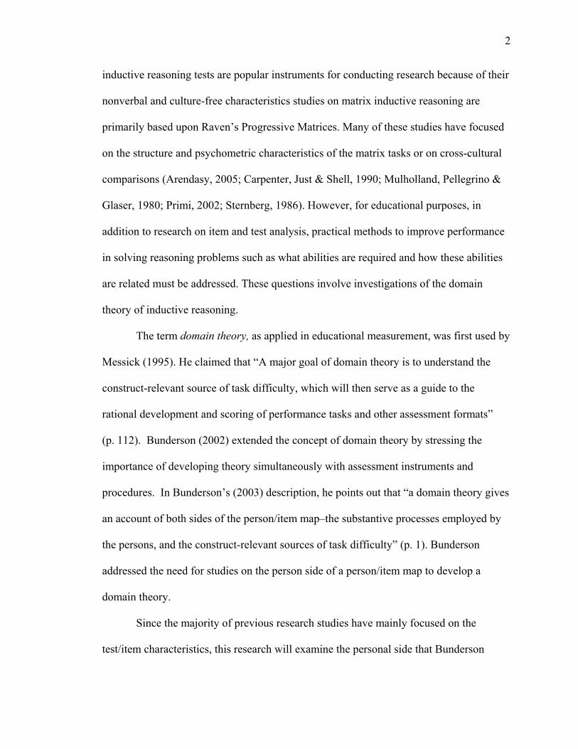
inductive reasoning tests are popular instruments for conducting research because of their
nonverbal and culture-free characteristics studies on matrix inductive reasoning are
primarily based upon Raven’s Progressive Matrices. Many of these studies have focused
on the structure and psychometric characteristics of the matrix tasks or on cross-cultural
comparisons (Arendasy, 2005; Carpenter, Just & Shell, 1990; Mulholland, Pellegrino &
Glaser, 1980; Primi, 2002; Sternberg, 1986). However, for educational purposes, in
addition to research on item and test analysis, practical methods to improve performance
in solving reasoning problems such as what abilities are required and how these abilities
are related must be addressed. These questions involve investigations of the domain
theory of inductive reasoning.
The term domain theory, as applied in educational measurement, was first used by
Messick (1995). He claimed that “A major goal of domain theory is to understand the
construct-relevant source of task difficulty, which will then serve as a guide to the
rational development and scoring of performance tasks and other assessment formats”
(p. 112). Bunderson (2002) extended the concept of domain theory by stressing the
importance of developing theory simultaneously with assessment instruments and
procedures. In Bunderson’s (2003) description, he points out that “a domain theory gives
an account of both sides of the person/item map–the substantive processes employed by
the persons, and the construct-relevant sources of task difficulty” (p. 1). Bunderson
addressed the need for studies on the person side of a person/item map to develop a
domain theory.
Since the majority of previous research studies have mainly focused on the
test/item characteristics, this research will examine the personal side that Bunderson

3
addressed in domain theory. This study will further investigate the nature of the abilities
required to solve Matrix Reasoning problems and the relationships among these abilities.
Background
In general, inductive reasoning is a process of drawing conclusions based on
observations and a hypothesis. It may involve applying existing knowledge to predict a
new instance in real life. Among the various tests which measure inductive reasoning
ability, Raven’s Progressive Matrices are consensually accepted as the quintessential test
of inductive reasoning (Alderton & Larson, 1990).
The format of items in Raven’s test is a geometric reasoning problem. Matrix
tasks are visual analogy puzzles; each matrix task usually consists of several figures
arranged in rows and columns with the last part missing. Corresponding figures or figural
parts are organized according to a certain rule. The dimensions of each matrix can be 2
by 2, 2 by 3, 2 by 4, 3 by 3, or larger. In these entries, geometric shapes, lines, and
background textures vary in form, number, orientation, and color. More than one rule
may be used in the figures. Students must identify the existing relationship in the
complete rows or columns, and then use that relationship to infer the missing entry in a
new row. Using a variety of shapes, figure combinations, or rules, items with different
difficulties can be created. Figure 1 is an example of Matrix Inductive Reasoning task.
The Raven’s test was developed to measure two complementary components of
general intelligence. Raven’s two components include (a) the ability to think clearly and
make sense of complex data, which is known as eductive ability, and (b) the ability to
store and reproduce information, known as reproductive ability. Researchers have
identified that Raven’s tests are the most g-loaded of existing intelligence tests. Since

4
Figure 1. Example of a Matrix Inductive Reasoning task

5
Spearman has defined general intelligence as a unidimensional construct, and Raven’s
tests have been used to measure g, many have made the assumption that Raven’s tests are
unidimensional, meaning that they measure only one kind of ability. However, if there is
only one kind of ability, what is this ability? How may one achieve it? Carpenter, Just,
and Shell’ (1990) research provided an alternative answer. In their research, Carpenter et
al. found the following process is required to solve Raven’s test problems: visual
encoding, finding the rule, and goal management (managing problem-solving goals in the
working memory). Based on an accumulation of data, the aforementioned Matrix
Reasoning problems, and literature reviews, colleagues at the Edumetrics Institute
identified four abilities that are needed to solve Matrix Inductive Reasoning problems.
These include the ability to (a) decompose the figure into parts, (b) find the rules, (c)
apply the rules, and (d) remember previous steps. The question of how these specific
component abilities work in combination with each other to produce matrix inductive
reasoning is the focal issue of this research.
Rationale for This Study
Although Raven’s test has received more attention than other matrix reasoning
tests (Arendasy, 2005; Carpenter et al., 1990; Embretson, 1995; Green et al., 2001;
Hornke & Habon, 1986; Mulholland et al., 1980), scholars have still not obtained
consistent results on important issues of its component constructs.
Most scholars have used factor analysis to explore the underlying structure of
Raven’s test. There is widespread disagreement over its constructs; some scholars
conclude that it is a unidimensional test, and that the only ability it measures is the
intelligence factor of g. Other scholars, on the other hand, claim that two or three factors
6
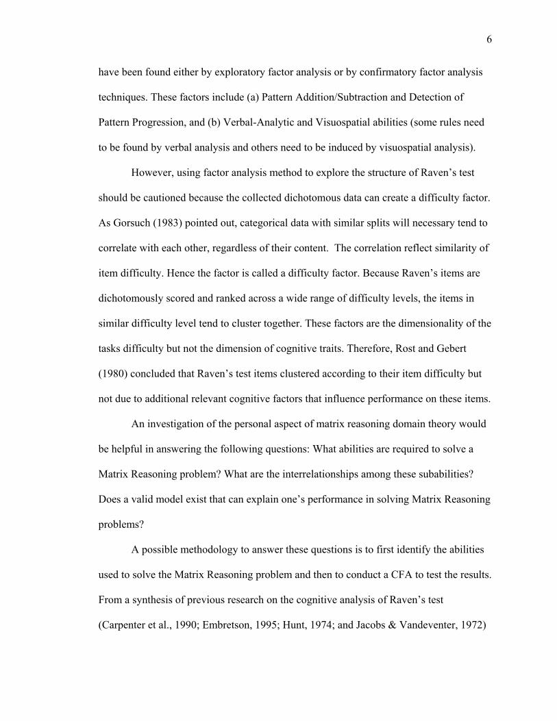
have been found either by exploratory factor analysis or by confirmatory factor analysis
techniques. These factors include (a) Pattern Addition/Subtraction and Detection of
Pattern Progression, and (b) Verbal-Analytic and Visuospatial abilities (some rules need
to be found by verbal analysis and others need to be induced by visuospatial analysis).
However, using factor analysis method to explore the structure of Raven’s test
should be cautioned because the collected dichotomous data can create a difficulty factor.
As Gorsuch (1983) pointed out, categorical data with similar splits will necessary tend to
correlate with each other, regardless of their content. The correlation reflect similarity of
item difficulty. Hence the factor is called a difficulty factor. Because Raven’s items are
dichotomously scored and ranked across a wide range of difficulty levels, the items in
similar difficulty level tend to cluster together. These factors are the dimensionality of the
tasks difficulty but not the dimension of cognitive traits. Therefore, Rost and Gebert
(1980) concluded that Raven’s test items clustered according to their item difficulty but
not due to additional relevant cognitive factors that influence performance on these items.
An investigation of the personal aspect of matrix reasoning domain theory would
be helpful in answering the following questions: What abilities are required to solve a
Matrix Reasoning problem? What are the interrelationships among these subabilities?
Does a valid model exist that can explain one’s performance in solving Matrix Reasoning
problems?
A possible methodology to answer these questions is to first identify the abilities
used to solve the Matrix Reasoning problem and then to conduct a CFA to test the results.
From a synthesis of previous research on the cognitive analysis of Raven’s test
(Carpenter et al., 1990; Embretson, 1995; Hunt, 1974; and Jacobs & Vandeventer, 1972)

7
and practical experience by a research team at the EduMetrics Institute, four ability
factors which affect individual differences in Matrix Reasoning problems have been
identified (a) figural decomposition ability, (b) rule induction ability, (c) deduction ability,
and (d) working memory capacity. A series of hypotheses on the relationship of these
will be proposed and empirically tested. The structural equation modeling (SEM) method
will be used to test these hypothesized models.
Purpose and Research Questions
Based on this review, the main purpose of this project was to further investigate
the process used to solve Matrix Reasoning problems. This research addressed the
following questions:
1. Which of several alternative models is the best representation of the domain of
Matrix Reasoning problem solving?
2. What modifications can be made to improve the model?
3. What are the significant direct and indirect effects of latent variables?
The predicted results of these questions indicate the existence of a valid model of
matrix inductive reasoning ability. This model can help designers design better ways to
assess progress and improvement in this sort of thinking, which can in turn help students
to diagnosis problems they experienced when given a matrix problem.
The significance of this research lies in the investigation of the domain theory of
matrix inductive reasoning from a cognitive process view, which will clarify which
abilities are needed to solve these matrix tasks. It will further assist in developing
instruments to improve performance in solving Matrix Inductive Reasoning problems.

8
Chapter 2: Review of the Literature
This study is an effort to understand the domain theory of matrix inductive
reasoning from an empirical study. Literature review on previous studies will address
how the domain of matrix inductive reasoning has been studied and what the connections
are between past studies and the questions raised in this research.
Issues Pertaining to a Domain Theory
To understand the concept of domain theory, we must first define the concept
domain. According to McShane (1991), a domain denotes “a collection of tasks that share
a common representation system and a common set of procedures for operating on these
representations to perform tasks” (p. 256). Thus, tasks which share common
representation systems and common problem solving processes may be considered a
domain. For example, number series completion is a domain of inductive reasoning, as
are verbal analogies and geometric analogies. In this work, when we speak of the domain
of matrix inductive reasoning we are referring to a broad collection of reasoning tasks,
that spans a variety of stimulus formats and difficulty levels that all involve drawing
inferences about the characteristics of a missing geometric figure in the context of a
particular pattern that the examinee is expected to observe.
The concept of domain theory was first used by Messick (1995) to define
construct validity:
A major goal of domain theory is to understand the construct-relevant
sources of task difficulty, which then serves as guide to the rational
development and scoring of performance tasks and other assessment

9
formats. At whatever stage of its development, the domain theory is a
primary basis for specifying the boundaries and structure of the construct
to be assessed. (p. 745)
Bunderson (2003) has broadened the concept of domain theory in the realm of
human learning and instruction:
Domain Theory (or learning theory of progressive attainments) is a
descriptive theory of the contents, substantive processes, dimensional
structure, and boundaries of a domain of human learning or growth that
give an account of construct-relevant sources of task difficulty, and
conjointly, an account of the substantive processes operative in persons at
different levels of learning or growth along the scale(s) that span the
domain. (p. 1)
This definition expands Messick’s notion of domain theory as the boundaries and
structure of a construct set by adding multiple dimensions and thinking processes. It also
requires the assessment instrument to be associated with learning by stage (progressive
attainments). At this point, a domain theory has connected tasks, processes, and learning
locations along one or more measurement the same scales. Literature on aspects of the
matrix inductive reasoning domain theory will be reviewed in the following sections.
General Introduction to Matrix Inductive Reasoning
Matrix inductive reasoning is a task type used to measure inductive reasoning
ability. It is designed by following the central idea of inductive reasoning: reaching a
general conclusion or overall rule based on limited observations. Raven’s series
progressive matrices are the most prominent examples of this type of test and are the

10
most widely used non-verbal intelligence tests. Due to the high loading of its items on the
general g factor, the Raven’s test is considered to be one of the most g-loaded tests in
existence.
Matrix Inductive Reasoning items are composed of figures. Subjects are asked to
determine the patterns shown in these figures and infer the missing figure by applying the
pattern to a new situation. Items are organized as 2 by 2, 3 by 3, 2 by 3, or 2 by 4
matrices. Generally the last entry of the matrix is generally empty, requiring the subject
to deduce the answer. The components of figures in each entry include geometric shapes,
shade, lines, and backgrounds. For the colored Raven’s test, color is another component
of the figures. These components vary in amount, form, color, position, and orientation in
entries along the same row or column. Figure 1 is an example of a 3 by 3 inductive
reasoning matrix.
In this example, there are 9 cells in the matrix with the last cell is empty. The
subject is required to select an answer from the options provided. The subject must
determine the relationship of components in the rows (or columns). For this example, we
can see that there are different shapes—triangle, circle, and hexagon—distributed in the
first two rows and the first two columns. The last entry is missing. From this observation,
we can hypothesize that rule governed in each line or column is a distribution of three
different shapes. Based on this hypothesized rule, the last entry should be one among the
three shapes which is different from the other two shapes in the last row and the last
column. Thus, the only option for the last entry is the circle. Therefore, option 1 is the
correct answer.

11
As we go through the process of solving a matrix problem, we notice that one of
the most important steps is finding the relationships or rules that govern the item.
Researchers have done substantial work in exploring possible rules to develop these
matrix questions (Arendasy, 2005; Carpenter et al., 1997; Hornke & Habon, 1986; Jacobs
& Vandeventer, 1972; Primi, 2002; Ward & Fitapatrick, 1973). A list of selected rules
which has been used in the past by researchers is listed in Table 1.
Item Difficulty Resources of Matrix Inductive Reasoning Problems
In order to design and develop different sources and levels of difficulty, the first
task is to discover complexity factors underlying tasks. Studies on what characteristic of
the items determines the item difficulty have been widely conducted. Matrix Inductive
Reasoning item difficulty has been studied from the views of the problem solving process,
the design experiment, and psychometric model analysis.
As Lohman (2002) points out that “Understanding what makes a task difficult is
not the same as understanding how participants solve items on the task, but it is a useful
place to start” (p. 225). The following researchers analyzed task difficulty by starting
from an analysis of the inductive reasoning problem solving process.
According to an analysis by Carpenter et al. (1990) of the process of problem
solving, the processes that distinguish individuals are primarily the ability of goal
management and the ability of rule inducing. Goal management is the management of a
large set of information in working memory. Rule inducing ability refers to discovering the
rules that correspond to the figures and it is influenced by the rule type. Carpenter et al.
also found that the error rate on a given problem was related to the types of rules and the
number of rules involved. A simple conclusion based on the work of Carpenter et al. is that

12
Table 1. Rules for the Solutions of Solving Matrix Inductive Reasoning Problems Rule Taxonomy Example
Constant in a row
The same value occurs throughout a row, but changes down a column.
Distribution of three values
Three values from a categorical attribute (such as figure type) are distributed through a row
Quantitative pairwise progression
A quantitative increment or decrement occurs between adjacent entries in an attribute such as size, position, or number
Figure addition or subtraction
A figure from one column is added to (juxtaposed or superimposed ) or subtracted from another figure to produce the third
Distribution of two plus one
Two same values and one different from a categorical attribute are distributed through a row (or column)
Distribution of two values
Two values from a categorical attribute are distributed through a row (or column); the third value is null.
Shading Change may be complete or partial
Size Proportionate change, as in photographic enlargement
Movement in a plane
Figure moves as if slid along surface
Flip-over Figure moves as if lifted up and replaced face down
(table continues)

13
Table 1 (continued)
Rule Taxonomy Example
Reversal
Two elements exchange some feature, such as size, shading , or position
Unique addition Unique elements are treated
differently from common elements, e.g., they are added while common elements cancel each other out
figure decomposition ability, rule induction ability, and the hierarchy of goals
management ability account for individual differences in performance in solving
geometric problems in the Raven’s test.
Mulholland, Pellegrino, and Glaser (1980) constructed 460 true-false analogies
with varying numbers of elements and transformations. The number of elements per item
varied between one and three; the number of transformations was between zero and three.
They found that the solution time is a direct function of the number of elements and the
number of transformations. This indicates that individuals decompose the patterns of an
analogy item sequentially by isolating the constituent elements one by one, as well as by
performing the transformations in a serial manner. It also shows that not the number of
elements, but only the number of transformations influences the percentage of errors.
Mulholland (1980) concluded that with an increasing number of elements and
transformations, it becomes more difficult to keep all of the performed steps in working
memory, whereby the number of required transformations contributes more to item
difficulty than the number of basic elements involved. An individual difference in the

14
ability to solve matrix analogy problems is then related to differences in working memory
capacity.
Green and Kluever (2001) conducted a components analysis of item difficulty in
Raven’s Matrices. She first identified 15 item components that might contribute to item
difficulty. They were (a) vertical or horizontal orientation versus other orientation (coded
as zero-1), (b) symmetrical versus asymmetrical (coded as zero-1), (c) progression versus
non-progression (coded as zero-1), (d) the number of dimensions in the pattern (coded as
zero-3), (e) straight lines versus curved lines (coded as zero-1), (f) the number of lines or
solids (coded as zero-1), (g) the density of design (coded as zero-1), and (h) color versus
black and white (coded as zero-1). Based on these characteristics, 60 items were
developed. Regression analysis was carried out with item difficulties as the dependent
variable and all of the 15 item characteristics were entered into a regression equation as
both forced entry and stepwise entry. We can see that most of the 15 characteristics are
figural characteristics. Another item difficulty was predicted based on the four
characteristics that were identified as significant predictors of item difficulty. The
multiple R2 was .69. However, there are some limitations to this research. For example,
this component analysis does not describe any elementary mental processes that may be
necessary for problem solutions; only very obvious and observable features have been
included in the analysis. However, the analysis of figural characteristics has provided
some information which can be used in test design and in item difficulty judgment. The
regression model used to predict new item difficulties has activated our concern that
using a regression model based on existing data to predict new item difficulties can only
provide fairly straightforward predictions.

15
Primi (2002) in his study synthesized four main factors from the literature (a) an
increase in the number of figures, (b) the perceptual complexity of stimuli, (c) the
complexity of the rules, and (d) an increase in the number of rules relating these figures.
The main purpose of Primi’s study was to identify the relative importance of the factors
listed above. By manipulating these four sources of complexity, the author created two
matrix tests to study the relative importance of these factors and their significant effect on
item complexity. Using ANOVA and regression analysis methods, the author identified
perceptual organization and the amount of information as the two variables which
contributed significantly to an increase in item complexity. Furthermore, perceptual
organization is the most important element, explaining 53.4% of the variance in item
complexity.
If the number of figures and the number of rules relating these figures are grouped
as one factor, we can see that there are three factors affecting the Matrix Inductive
Reasoning item difficulties. Named by Primi (2002), these three factors are (a) Amount
of Information Number of Elements and Rules, (b) the Nature of Relationships-type of
rules, and (c) Perceptual Organization.
Amount of information includes the number of attributes and the number of rules
involved in each figure; this is related to working memory capacity. When solving a
matrix problem, one needs to keep in mind how many elements there are in the figure and
what their relationships are. The more elements and rules the figure has, the larger
working memory capacity will be needed.
Rule type is another source which affects item difficulties. Easier rules such as
constants in a row (column) and a distribution of 3 can be easily identified with

16
perceptual identification. However, for the more difficult rules such as quantitative pair-
wise progression and figure addition, subjects need mental or conceptual operation in
addition to visual perceptual identification. Among these rules, the first six in Table 1
have received more attention than the others. However, the rule of distribution of two
values and the rule of figure addition/subtraction are in fact the same. As we can see in
the examples of these two rules, they both have two same values and a third non-value.
Therefore, in this research, we consider the distribution of two values and the figure
addition/subtraction rules as one: the distribution of two plus zero. Studies on the
difficulty of the rule found that the order of the five rules from easiest to hardest is
constant in a row (column), quantitative pair-wise progression, figure addition,
distribution of 3, and distribution of 2 plus 1 (Carpenter et al., 1990). These rules are
used in the Raven’s progressive matrices. In this research, we have also used these five
well-studied rules to design and develop Matrix Reasoning Tests.
Perceptual organization refers to how the figure is organized. The spatial order of
elements can include proximity, similarity, continuity, and with common region (Mack,
Tang, Tuman, & Rock, 1992), which add to the effect of the figure overlay distortion and
fusion (Embretson, 1998). If one object is on the top of another, the drawing feature is
called overlay; if two objects are put side by side with a common region in the same array
location, the drawing feature is called fusion; if an ordinary shape is perceptually altered,
bended, twisted, or stretched, etc., the drawing feature is called distortion. These features
will distort the clues and make the items more difficult.
By balancing the three sources of difficulty, Matrix Reasoning Tests with range of
difficulty distribution may be easily designed and developed.
17
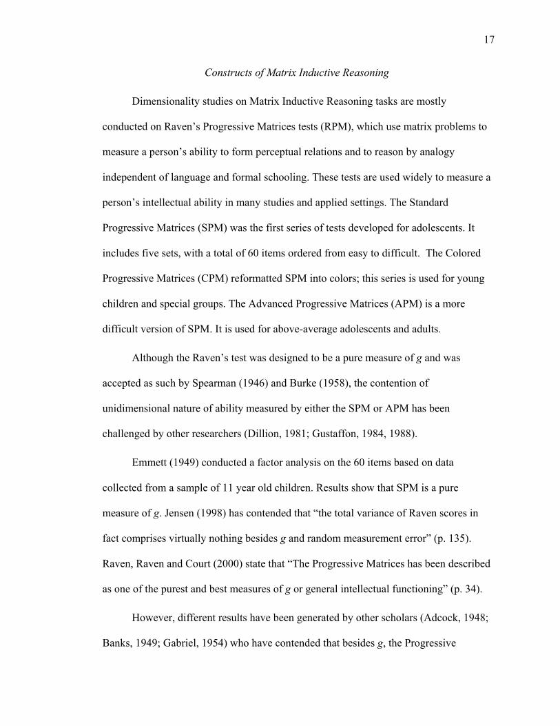
Constructs of Matrix Inductive Reasoning
Dimensionality studies on Matrix Inductive Reasoning tasks are mostly
conducted on Raven’s Progressive Matrices tests (RPM), which use matrix problems to
measure a person’s ability to form perceptual relations and to reason by analogy
independent of language and formal schooling. These tests are used widely to measure a
person’s intellectual ability in many studies and applied settings. The Standard
Progressive Matrices (SPM) was the first series of tests developed for adolescents. It
includes five sets, with a total of 60 items ordered from easy to difficult. The Colored
Progressive Matrices (CPM) reformatted SPM into colors; this series is used for young
children and special groups. The Advanced Progressive Matrices (APM) is a more
difficult version of SPM. It is used for above-average adolescents and adults.
Although the Raven’s test was designed to be a pure measure of g and was
accepted as such by Spearman (1946) and Burke (1958), the contention of
unidimensional nature of ability measured by either the SPM or APM has been
challenged by other researchers (Dillion, 1981; Gustaffon, 1984, 1988).
Emmett (1949) conducted a factor analysis on the 60 items based on data
collected from a sample of 11 year old children. Results show that SPM is a pure
measure of g. Jensen (1998) has contended that “the total variance of Raven scores in
fact comprises virtually nothing besides g and random measurement error” (p. 135).
Raven, Raven and Court (2000) state that “The Progressive Matrices has been described
as one of the purest and best measures of g or general intellectual functioning” (p. 34).
However, different results have been generated by other scholars (Adcock, 1948;
Banks, 1949; Gabriel, 1954) who have contended that besides g, the Progressive

18
Matrices also measure a small factor of Visualization or Space. Gustaffson (1984, 1988)
concludes that SPM contains a reasoning factor and a figural related cognition factor.
Hertzog and Carter (1988) insist that SPM contains two factors: Verbal Intelligence and
Spatial Visualization. Van der Ven and Ellis (2000) hold that SPM contains two
significant factors which they identify as Gestalt Continuation and Analogical
Reasoning. Lynn, Allik, and Irwing (2004) find that the three-factor solution for SPM
can get the best fit of the data by using both exploratory factor analysis and
confirmatory analysis method. The three factors are Gestalt Continuation, Verbal-
Analytic reasoning, and Visuospatial Ability.
The same conflicting conclusions have been shown in the studies of APM.
Alderton and Larson (1990) and Arthur and Woehr (1993) have claimed that a single-
factor solution seems to be the best representation of the APM’s structure, which means
that APM is solely a measure of g. However, Dillon, Pohlmann, and Lohman (1981)
have identified two factors in their study of APM; they named the two factors Pattern
Addition/Subtraction and Detection of Pattern Progression. When Lim (1994) studied
gender differences in performing APM, he concluded that APM is a pure measure of
reasoning ability for boys, but that it also measures spatial ability for girls. Deshon,
Chan, and Weissbein (1995) found two factors that they identified as Verbal-Analytic
and Visuospatial abilities. Colom and Garcia-Lopez (2002) also conclude that the APM
test measures both reasoning and spatial abilities.
The above studies on factors of the Raven’s test have used factor analysis
statistical techniques. The factors from the results of factor analysis are items clustered in
groups according to their item difficulty. Difficulty factors are produced by the
19
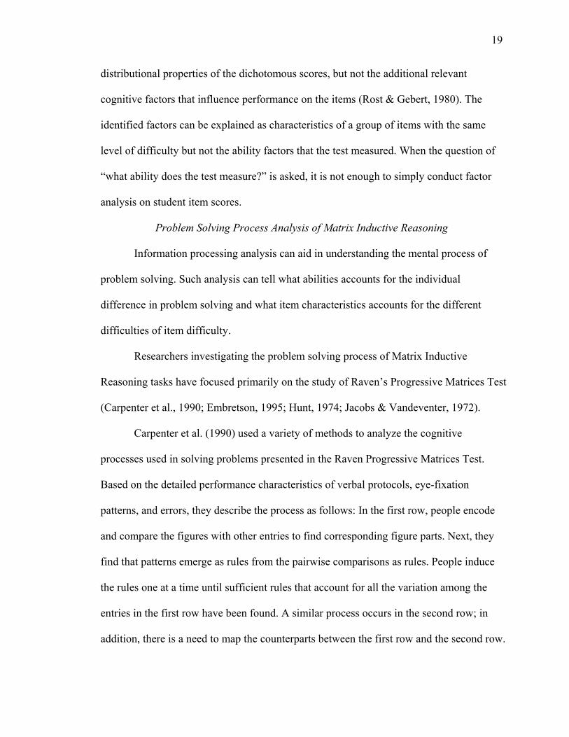
distributional properties of the dichotomous scores, but not the additional relevant
cognitive factors that influence performance on the items (Rost & Gebert, 1980). The
identified factors can be explained as characteristics of a group of items with the same
level of difficulty but not the ability factors that the test measured. When the question of
“what ability does the test measure?” is asked, it is not enough to simply conduct factor
analysis on student item scores.
Problem Solving Process Analysis of Matrix Inductive Reasoning
Information processing analysis can aid in understanding the mental process of
problem solving. Such analysis can tell what abilities accounts for the individual
difference in problem solving and what item characteristics accounts for the different
difficulties of item difficulty.
Researchers investigating the problem solving process of Matrix Inductive
Reasoning tasks have focused primarily on the study of Raven’s Progressive Matrices Test
(Carpenter et al., 1990; Embretson, 1995; Hunt, 1974; Jacobs & Vandeventer, 1972).
Carpenter et al. (1990) used a variety of methods to analyze the cognitive
processes used in solving problems presented in the Raven Progressive Matrices Test.
Based on the detailed performance characteristics of verbal protocols, eye-fixation
patterns, and errors, they describe the process as follows: In the first row, people encode
and compare the figures with other entries to find corresponding figure parts. Next, they
find that patterns emerge as rules from the pairwise comparisons as rules. People induce
the rules one at a time until sufficient rules that account for all the variation among the
entries in the first row have been found. A similar process occurs in the second row; in
addition, there is a need to map the counterparts between the first row and the second row.

20
These rules are stored in the memory in a generalized form. The discovered rules are then
applied to the third row to generate the missing entry.
Beginning with a task analysis of Raven’s Progressive Matrices Test, Carpenter et
al. (1990) found that five different types of rules govern the variation of the entries. These
rules are always interchangeable in the same task. For a single rule, the difficulty order of
the five types is (a) constant in a row where the same value occurs throughout a row but
changes down a column, (b) quantitative pairwise progression where a quantitative
increment or decrement occurs between adjacent entries in an attribute such as size,
position, or number, (c) figure addition or subtraction where a figure from one column is
added to (juxtaposed or superimposed) or subtracted from another figure to produce the
third, (d) distribution of three values where three values from a categorical attribute are
distributed through a row, and (e) distribution of two values where two values from a
categorical attribute are distributed through a row; the third value is null.
If a problem involves multiple rules, subjects use a correspondence finding method
to discover which elements in three entries in a row are governed by the same rule. Since
cues for finding rules are ambiguous in some of the Raven’s problems which are
constructed by conjoining figures governed by several rules, the correspondence finding
process is thus a source of difficulty.
Carpenter et al. (1990) furthermore claimed that Raven’s item difficulty also varies
with the number of rules. However, a large number of rules do not have a large effect on
the process of inducing rules. Instead, the number of rules affects the goal-management
processes that are required to construct, execute, and maintain a mental plan of action
during the solution of the multiple rule problems. Carpenter et al. used two experiments to

21
test this hypothesis. The purpose of Experiment 1 was to reveal the process and the content
of thought when subjects were solving each Raven problem. Think aloud and eye fixations
methods were applied to some subjects. Other subjects were asked to work silently and
then describe the rules that stimulated their response. The results from both groups showed
the incremental nature of the processing: the subjects solved a problem by decomposing it
into successively smaller sub-problems and then proceeded to solve each sub-problem one
at a time.
Based on this result, the authors put forward the other hypothesis that a major
source of individual differences “is the ability to generate sub-goals in working memory, to
monitor progress toward attaining them, and to set new sub-goals as others are attained” (p.
413). The whole process of generating sub-goals, monitoring progress, and setting up new
goals is called goal management. In Experiment 2, subjects were first administered the
Raven Progressive Matrices Test; they were then trained with the goal-recursion strategy to
solve the Tower of Hanoi puzzle task, a cognitive task involving extensive goal
management. Significant correlation between the two tasks leads to the conclusion that a
major source of individual difference in the Raven test derives from the generation and
maintenance of goals in working memory.
To specify the process required to solve the Raven problems, two simulation
programs were developed: FAIRAVEN performed at the level of the median college
student in the sample, and BETTERAVEN performed at the level of the best subjects in
the sample. These two models verified the results of Experiments 1 and 2. The authors
conclude that “what one intelligence test measures, according to the current theory, is the
common ability to decompose problems into manageable segments and iterate through

22
them, the differential ability to manage the hierarchy of goals and sub-goals generated by
this decomposition, and the differential ability to form higher level abstractions” (p. 429).
Another investigation on the information process of matrix problem solving was
conducted by Embretson (1995). Her study examined student performance on 150 matrix
items generated based on a cognitive theory of abstract inductive reasoning. The goal of
Embretson’s study was to estimate the relative contributions of individual differences in
general control processing and in working memory capacity to individual differences in
performance on these matrix items. Embretson (1995) attempted to distinguish the relative
importance of executive functions (Belmont & Butterfield, 1990) and the role of working
memory (Carpenter et al., 1990) by using a multi-component latent-trait model. Two latent
variables which were responsible for individual differences in the task were posited:
working memory capacity and control processing results showed that control process latent
variable accounting for more variance than the working memory latent variable.
While control processes played an important role for high levels of performance on
difficult reasoning tasks, Embretson’s (1995) also found that working memory or attention
resources also play important roles.
In conclusion, goal management process and working memory are important
aspects of the process of solving Matrix Reasoning problems.
Working Memory and Inductive Reasoning
The important role of working memory in solving inductive reasoning tasks has
been strongly claimed by many researchers (Carpenter et al., 1990; Marshalek et al.
1983). Buehner, Krumm, and Pick (2005) even proposed that reasoning is equal to

23
working memory. In this section, we will review studies on the relationship between
working memory and inductive reasoning.
Although it was first referred to as short-term memory, scholars now emphasize
the manipulative function of working memory. Researchers have proposed many
different models to explain the structure and function of working memory. Of them,
Baddeley’s (1992) model was taken as the most important influential one. Baddeley’s
(1992) model included three elements: (a) the visuospatial sketch pad which is a
visuospatial storage system, (b) the phonological loop which stores verbal based
information, and (c) the central executive system which is an attention-controlling system
and coordinator for the two storage components and their interactions. Working memory
is an important indicator of reasoning ability.
Kyllonen and Christal (1990) designed some working memory tasks specifically
used to measure Baddely’s concept of working memory. They found structural
coefficients of .80 through .88 in four large studies between working memory and
reasoning ability. Although Keyllonen’s et al. (1990) work was criticized that some of the
tasks for working memory test and reasoning test are the same thus increased the
correlation, the overall high correlation coefficients showed the strong relationship
between working memory and reasoning ability. Kyllonen and Christal (1990) argue that
all reliable variation in reasoning can be explained by limitations on working memory
capacity.
Conflicting results existed in other research. These researches emphasized the
important function of executive attention. Researchers argued that the shared variance
among measures of working memory span and complex cognition reflects primarily dues

24
to the contribution of executive function, rather than specific storage capacity (Engle &
Kane, 2004). As Kane, Hambrick, et al. (2004) pointed out,
correlations between WM [Working Memory] span and complex cognition are
jointly determined by general executive-attention and domain-specific storage but
primarily by executive attention. Thus, a WMC [Working Memory Capacity]
measure should be quite general in predicting cognitive function. That is, the
memory span test could be embedded in a secondary processing task that is
unrelated to any particular skill or ability and still predict success in a higher level
task. Evidence supporting this view comes from three sources: (a) manipulating
the processing demands of verbal WM [Working Memory] pan tasks and noting
their relations to comprehension, (b) examining the between verbal WM span and
measures of general fluid intelligence, and (c) examining the link between verbal
WM span and low-level attention capabilities. (p. 190)
Relationship between Raven’s Advanced Progressive Matrices in conjunction
with working memory was also examined by some researches. Jurden (1995) reported the
correlation of WM performance to the Raven reading span and computation span of .20
and .43 respectively. Babcock (1994) found a higher relationship of .55 between working
memory and Raven performance. Although these studies differed in the degree of
relationship reported, they both agree that working memory is positively correlated with
performance on the Raven’s test.
As a result, the author concluded that working memory should be tested by using
multiple facets. When solving Matrix Reasoning problems, people need to store the
identified rules governing the corresponding figure parts in their working memory. This

25
memory is related to the observed patterns and shapes. The goal management process is
also needed to control what information should be stored in the working memory and
what information should be released from memory. Considering that Matrix Reasoning
tasks are composed of figures, we chose two types of working memory tests that are
similar in regard to the memory functions discussed above. The two tests include the
Binary Number Working Memory Test (BNWMT) and the Shape Memory Test (SMT).
In the BNWMT, each item is a number containing a series of ones and zeroes such as
110110110 or 01100110. The task of the examinee is to identify and remember the
pattern of the digits. In the SMT, the memory tasks are a number of shapes that
examinees are expected to remember.
Above is a review of research related to the domain of matrix inductive reasoning.
These studies have provided the fundamental theories and raised questions for the further
research.

26
Chapter 3: Method
Chapter 3 discusses the methods used to conduct this research. It introduces how
the instrument was developed to measure the matrix reasoning abilities and the
subabilities. The process of obtaining samples and collecting data are also elaborated.
Procedures for analysis the data is then laid out. The chapter also includes the methods
used to address each research question.
Instrument Development
Five tests were developed to measure the subablities identified from the previous
discussion. Each of them is described in detail below.
Matrix Reasoning Test
A 16-item Matrix Reasoning Test was constructed to measure the matrix
inductive reasoning ability. It was patterned after Raven’s series of tests. The format and
content of this new test is described in the following sections.
Item format. Each matrix item consisted of nine entries arranged in three rows and
three columns. The last entry on the lower right contained a question mark; all other
squares were figures. There were six answer options for each matrix item. Subjects were
asked to choose one correct answer from the six options to complete the blank entry. An
example of such a matrix item is shown in Figure 1.
Item content specifications. The matrix items were constructed by varying the
four aspects which affected the difficulty of the items (a) the number of elements, (b)
number of rules, (c) rule types, and (d) figural complexity. The five rules used in the tests
included (a) constant in a row (column), (b) distribution of two values plus zero, (c)

27
distribution of two values plus one, (d) quantitative progression, and (e) distribution of
three. The constant in a row rule was that the same attribute occurs throughout a row (or a
column); the rule of distribution of two values plus zero was that two identical values are
distributed through a row while the third value is none; the rule of distribution of two
values plus one was that three values from a category attribute distributed through a row
with two of the three values are identical while the third one was different from the other
two; the quantitative progression rule was that a quantitative increment or decrement of a
value occurs between the two adjacent entries. To further understand these rules in the
items, refer to Table 2 for content specification. In this table, rules were listed in the first
row while items were listed in the first column. The number 1 in the cross cells means
that the rule in this column has been used once in the item. If more than one number 1
appears in the cell, it shows that the rule in this column has been used more than once.
Rule Induction Test
The purpose of the Rule Induction Test was to determine how well the examinees
discover or recognize a particular rule. Without the interaction of other factors such as
complex figural or multiple elements, could the subjects figure out what the rule was?
At the top of the page, two rows of simple figures were given to the subjects.
Figures in these two rows were governed by the same rule. Four options were listed after
the instruction. One or more of the options shared the same rule as the previous two. The
subjects were asked to choose the one or more options which shared the same rule as the
previous two rows. Refer to Figure 2 for an example of the Rule Induction task. In this
test, each items used a different single rule.

28
Table 2.
Rule Types and Number of Rules Used in Matrix Reasoning Test
Rule Type* Constant 2+0 2+1 Quantitative D3
Rules in Each
Item
1 1 1
2 1 1
3 1 1
4 2 2
5 1 1 2
6 1 1 2
7 1 2 3
8 1 2 3
9 2 2
11 1 1 2
12 2 2
13 1 1 1 3
14 1 2 2 4
13 3 3
16 3 3
*constant: constant in a row (or column); 2+0: distribution of two plus zero (figure
addition); 2+1: distribution of two plus 1. Quantitative: quantitative progression.D3:
distribution of three.

29
Figure 2. Example for a Rule Induction Test item.

30
Rule Application Test
The Rule Application Test was used to examine subjects’ ability to apply a rule to
a new situation. In this test, the researcher first decomposed the figures. A clear rule
description for a particular part of the figure was then was provided. Two figures were
given; the subjects were asked to find out what the third one should be by applying the
rules provided. Figure 3 is an example of a Rule Application item.
Table 3 presents the rule types and the number of rules used in each item of the
Rule Application Test.
Working Memory Test
This test focused on working memory capacity. It included two parts: the
BNWMT and the SWMT.
Binary Number Working Memory Test. This test asked subjects to remember
several binary numbers ranging from 3 to 12 digits. The ratio of number length/display
time was 1:1. For example, for a 3-digit number, the display time is 3 seconds; for a 4-
digit number, the display time is 4 seconds, and so on. The binary number was shown in
the first page, then automatically went to the answer page after the display time expired.
In the answer page, the subjects needed to type in the number they saw on the previous
page. There were 10 items. One example of an 8-digit binary number was 10010101.
Shape Working Memory Test. SWMT asked subjects to remember the shapes they
saw on a previous page. These shapes were regular geometric shapes. The number of
different shapes in each item ranged from three to nine. The shapes were displayed for a
fixed time interval; then an answer page was displayed. The subjects were asked to

31
rule1: For the outside part: two shapes are the same,
the third one is none.
rule2: For the inside part: two shapes are the same,
the third one is none.
Figure 3. Example of a Rule Application Test item.

32
Table 3.
Rule Types and Numbers Used for Each Item in Rule Application Test
Rule Type* Constant 2+0 2+1 Quantitative
D3 1 1
2 1 1
3 Bad item 1
4 2
5 1 1
6 1
7 3
8 3
9 1 1
10 1 1
11 1 1 1
* constant: constant in a row (or column); 2+0: distribution of two plus zero (figure
addition); 2+1: distribution of two plus 1. Quantitative: quantitative progression.D3:
distribution of three.
choose figures they saw from a list of 20 shape options. The ratio between the numbers of
shapes and the display time was 1:1.5. The following is an example of a three SWMT
item:
Figure Detection Test
The Figure Detection Test was used to measure figural decomposition ability.
For complex figures in the Matrix Reasoning tasks, subjects were asked to decompose

33
them to independent parts and find the correspondence rule among the figures. The
Figure Detection Test used the format of Hidden Figure tasks. In this test, subjects were
asked to find a given shape which was embedded in a complex one. Figure 4 shows an
example of a Figure Detection item that was used in this research.
Sampling
Structural equation modeling is sensitive to sample size and requires relatively
large sample sizes. The sample should consist of a minimum of 100 subjects and should
be at least five times larger that the number of variables being analyzed (Bantler & Chou,
1987). Because the number of test items developed in this research was 52, at least 260
subjects should be included according to the minimal sample size rule.
Students from grade 6 through grade 8 participated in this study. These students
were from Beijing and Shanghai. Items in this research were developed from Colored
Progressive Matrices and the Advanced Progressive Matrices, being more difficult than
the Colored Progressive Matrices, yet easier than the Advanced Progressive Matrices.
According to Raven’s test, Colored Progressed Matrices are used with younger children
And special groups and the Advanced Progressive Matrices are used with above teachers,
and students. The four principals, ten teachers, and each student in the selected classes
who agreed to participate in the research were asked to sign an agreement form.
Data Collection
To collect the data, a database was developed by using the PHP and MySql
computer languages. The five tests were then connected to the database. The database
was stored in the computer lab servers in the two participating schools in Beijing and

34
A B C D
Figure 4. Example of a Figure Detection Test item.

35
Shanghai. The five tests were administered to whole group of students over the internet
on each campus to one classroom at a time. Trained graduate students were in the
computer lab on each campus to assist the students in completing the tests. No time limit
was imposed. Students completed the test during the last class period of the school day
and were able to respond to each test at their own pace. All the collected data were stored
on the computer lab servers of participating schools.
Pilot Study Data Collection
A pilot study was conducted with a small group of students before the tests were
administered to the full sample of students. The purpose of this pilot study was to
examine item characteristics. Further actions including modifying, deleting, and adding
items to the test were adopted based on pilot study analysis results. One hundred and
eleven students from grade 7 participated in the pilot study. Of the 111 students, 53
(47.7%) were female, 54 (48.6%) were male. Four students (4.3%) did not report their
gender. Seventy eight (70.3%) of the 114 students were age 12, 27 (24.3%) were age 13,
and 6 (5.4%) students did not report their age.
Items were deleted and added based on the item difficulties from the pilot study.
Table 4 illustrates the item changes for each individual test.
Formal Data Collection
The revised tests were administrated to a sample of 352 students in China from
grades 6 to 8. Students who participated in the pilot study were not included in the data
collection. The same data collection procedure that was used in the pilot study was
adopted for use in the general sample data collection. Table 5 shows student
participation numbers and rates by grade and gender.

36
Table 4.
Item Changes in the New Test
Tests Number of
Items Deleted Number of
Items Added Number of Items in the New Test
Binary Number Working Memory Test 4 2 5
Shape Working Memory Test 1 0 4
Figure Detection Test 4 0 4
Rule Induction Test 0 0 6
Rule Application Test 0 0 12
Matrix Reasoning Test 2 0 14
Upon receipt, the data was inputted into Microsoft Excel. Under the supervision
of a graduate student, the inputted data was carefully checked for errors to ensure
accuracy. After the data was considered clean, analyses were conducted.
Data Analysis
Scoring and Data Cleaning
Through the use of Microsoft Excel logical functions, the initial answers of
students were scored with either a 1 (correct) or a 0 (incorrect) and saved in a different
data file. In the data collection process, instances of missing data were encountered. If
any of the items in one or more of the five tests were not completed, the case was directly
eliminated from the analysis. Of the 352 participants, 18 cases were eliminated. The
analysis of this study is based upon the remaining 334 complete effective cases.

37
Table 5. Student Participation Numbers and Rates by Grade Enrollment and Gender Data input
Gender Grade
Number of participants Males Females Unkown
6 117 (35.03%) 49 (14.67%) 65 (19.46%) 3 (.90%)
7 116 (34.73%) 52 (15.57%) 58 (17.37%) 6 (1.80%)
8 100 (29.94%) 39 (11.68%) 59 (17.66%) 2 (.60%)
Null 1 (.30%) 0 (0.00%) 0 (0.00%) 1 (.30%)
Total 334 140 (41.92%) 182 (54.49%) 12 (3.59 %)
Software Selection
Many software packages were available for the modeling analysis. The most
commonly used are AMOS (Arbuckle, 2003; Arbuckle & Wothke, 1999; SPSS, Inc.,
2005), LISREL (Jöreskog & Sörbom, 1996; Jöreskog, Sörbom, Du Toit, & Du Toit,
2001), and MPLUS (Muthen & Muthen, 2001). Of these software packages, MPLUS is
the most well known for its capacity to deal with complicated models, handling both
continuous and categorical data. Using proper estimation methods such as analyzing
tetrachoric correlations and using a robust unweighted or weighted least-squares
estimator, MPLUS can conduct both EFA and CFA with dichotomous data. Since the
data used in this research is dichotomous, MPLUS was used in this research.

38
Reliability and Validity
Cronbach’s alpha coefficient was computed to estimate the internal consistency
reliability of the scores obtained from each test. Evidence of convergent validity was
obtained by examining the factor coefficients (Anderson & Gerbing, 1988). Convergent
validity is demonstrated if the items which are associated have significant high
coefficients (greater than twice its standard error) on the same factor and if the factor
loading is relatively high (greater than .06). Evidence of discriminant validity was
confirmed by showing that the confidence intervals (± two standard errors) around the
estimated correlation coefficients for a given pair of factors contained the value of 1.0.
Measurement of Construct for each Test
To explore the constructs of the developed tests, CFA models based on related
literature and theories were tested. Three models were specified for each test (a) a
unidimensional model in which all of the items using different type and number of rules
and figures were represented by a single factor; (b) a first-order oblique model that
included separate factors for items in different difficulty levels; and (c) a second-order
factor model used to account for covariation among factors. For each test, the
unidimensional model was first tested. Only if this unidimensional model did not fit the
data acceptably would the other two models be tested. Otherwise, this unidimensional
model would be applied to the following structural equation modeling analysis.
The CFA analysis was conducted using MPLUS. As mentioned in the preliminary
research by Muthén, DuToit, and Spisic (1997), an optimal estimation method for
categorical outcomes was weighted least-squares with mean and variance adjustment

39
(WLSMV). Since the data in this research was dichotomous, the WLSMV estimation
method was the best choice.
To evaluate the fit of each model, a combination of criteria consisting of chi-
square tests and several descriptive fit indices were adopted. The chi-square test is a basic
statistical procedure to test for model fit. A nonsignificant chi-square value indicates
good model fit. The chi-square test is sensitive to sample size, being particularly hard to
obtain with a large sample size. Besides the chi-square test, MPLUS also provided the fit
indices of the comparative fit index (CFI), the Tucker-Lewis index (TLI), the
Standardized Root-Mean-Square Residual (SRMR), the Weighted Root Mean Square
Residual (WRMR), and the Root Mean Square Error of Approximation (RMSEA). Of
these indices, SRMR is not recommended for dichotomous data (Yu, 2002). Therefore,
CFI, TLI, RMSEA, and WRMR were chosen for the construct analysis for each
individual test. For the model test which using continuous data, SRMR is adopted instead
of WRMR. CFI measured the improvement of the fit by comparing the hypothesized
model with a null model in which the measured variables were assumed to be unrelated
(Bentler & Bonett, 1980). Hu and Bentler (1999) recommended a CFI cutoff value of
around .95. RMSEA shows the average difference between observed and expected
covariance; a RMSEA value below .05 indicates a good model fit (Browne & Cudeck,
1993).WRMR was proposed by Muthén and Muthén (1998-2001) as being suitable with
non-normal outcomes. A model is accepted when the WRMR value is equal to or less
than 1.0 for the model (Yu, 2002). Cut off values equal or less than .08 was recommend
by Yu (2002) in her research. In summary, joint criteria for a good fit of indices
according to this study are CFI ≥ .95, RMSEA ≤ .05, and WRMR ≤ 1.00 or SRMR ≤ .08.

40
Research Questions and Methods
Research questions and the corresponding methodologies are addressed in this
section.
Research Question 1: Which of the Alternative Models is the Most Valid Representation
of the Domain of Matrix Reasoning Problem Solving?
In line with the three theoretical hypotheses regarding the domain of Matrix
Reasoning problem solving referred to earlier, three alternative models (Figures 5 to 7)
were defined. The common part of the three models was that the four predictor variables,
working memory, figural decomposition, rule induction, and rule application, had direct
effects on matrix reasoning.
The first model (Figure 5) is a component model. In this model, in addition to its
direct effect on matrix reasoning, working memory also directly affects figure detection,
rule induction, and rule application. Each of these three variables also predicts matrix
reasoning.
All other variables in the second model (Figure 6) directly affect the matrix
reasoning variable. Also, working memory, rule induction, and figure detection indirectly
affect matrix reasoning through the mediator variable rule application. There are no
relationships specified among the latent variables figure detection, working memory, and
rule induction.
The third model (Figure 7) tests the problem solving process theory. Working
memory directly affects all other variables. Simultaneously, a step-by-step process is
required from figure detection to rule induction, rule induction to rule application, and
finally from rule application to matrix reasoning.

41
Figure 5. Hypothesized model 1: component model.
Working Memory
Matrix Reasoning
Figure Detection
Rule Induction
Rule Application

42
Figure 6. Hypothesized model 2: rule application as mediator model.
Working Memory
Matrix Reasoning
Figure Detection Rule
Induction
Rule Application

43
Figure 7. Hypothesized model 3: problem solving process model.
Working Memory
Figure Detection
Rule Induction
Rule Application
Matrix Reasoning

44
The three models were combined into a full model in which all latent variables
were intercorrelated with each other. The model which fits the actual data with the
greatest degree of accuracy would be preferred.
Data preparation for the model analysis. Structural equation modeling (SEM)
was used to evaluate the three hypothesized models. SEM is a family of statistical
techniques that includes path analysis and factor analysis. It can be used to test the
plausibility of hypothesized patterns of causal effects involving latent variables. There are
two ways to prepare the data for SEM analysis. One way is to export the chosen
constructs with the original items to the model. The second way is to create scales by
adding up item scores under the same factor. For tests with unidimensional construct, a
parcel was used to create two or more observed variables. Because the second method is
parsimonious and has fewer errors, the second method was adopted.
Procedure to test the models. To test the structural equation models, a two-step
modeling method introduced by Anderson and Gerbing (1988) was adopted.
The first step is to respecify the structural equation models to a CFA measurement
model. Testing the validity of the measurement model before evaluating the structural
model allows the research to distinguish rejections of the proposed model because of
problems stemming from measurement inadequacies from problems related to the actual
proposed theory (Mueller, 1996). Since all SEM models share the same latent variables,
only one CFA model will be addressed. This measurement model expresses all possible
associations among the latent variables. It considers each observed indicator as a linear
combination of a latent unobserved factor plus random measurement error. Testing the
validity of the measurement model before evaluating the structural model allows the

45
research to identify problems stemming from measurement inadequacies (Mueller, 1996).
Since the variables in this model are continuous variables (scales), the Maximum
Likelihood (ML) estimation method was used for the model testing.
Given an acceptable CFA model, the second step is to test and compare the
proposed SEM models. The three SEM models were tested under the same available data
as used in the first step. Results from the MPLUS software for the three models were then
compared to the newly identified CFA model. As the method applied in the measurement
model analysis, Chi-square values and joint criteria for a good fit of indices of CFI & TLI
≥ .95, RMSEA ≤ .05, and WRMR ≤ 1.0 were obtained to evaluate whether the
hypothesized structural model is a valid representation of the domain constructs.
Research Question 2: What modifications can be made to improve the preferred SEM
model?
The model preferred in question 1 was theoretically specified. The MPLUS
program also provides a MODINDICES index which suggests empirical modifications to
improve the best model fit based on the actual data. The MODINDICES indices were
examined to see whether some reasonable suggestions could be made to the model in
question 1. If any modifications could be adopted, new modified models should be
retested.
Research Question 3: What Are the Significant Direct and Indirect Effects of the Latent
Variables?
Direct and indirect effects can be specified using the MPLUS program. All path
coefficients from the final model in question 2 were examined. These coefficients were
reported from MPLUS results. The outputs from MPLUS included the Estimates (the

46
model-estimated values for each parameter), the standard errors of the parameter
estimates, the values of the parameter estimates divided by the standard error, and two
types of standardized parameter estimates. MPLUS outputs did not provide p-values for
each estimated parameter. The ratio of the estimate divided by the standard error was
used to indicate the significance of the parameters. The ratio statistical test is an
approximately normally distributed quantity (z-score) in large samples. Values that
exceed +1.96 or fall below -1.96 are significant below p = .05 for a two-tailed test.
Conclusions were drawn based on these ratio values.
The relative strength of associations across latent variables can be reflected from
standardized parameter estimates. Of the two types of standardized parameter estimates,
the first type of coefficients are standardized using latent variable variance while the
second type of coefficients use the latent variables as well as the observed variable
variances. In this question, the two types of coefficients were the same because the
parameter estimates involved only latent variables.

47
Chapter 4: Results
Chapter 4 presents the findings of the study based on the data analysis. In this
chapter, the descriptive statistics for each test used in this study are reported followed by
detailed analysis on each of the research questions.
Test Score Reliability
Item internal consistency reliability estimates were calculated using SPSS. The
Cronbach’s alpha for each of the five tests is reported in Table 6. The Figure Detection
test had the lowest alpha value of .53. The alpha coefficient of .62 for the shape Working
Memory test was moderately low too. One reason for the low reliability estimates for
these two tests is that each of them included only four items. The lower reliability
estimates for these two tests indicate that interpretations about examinees based on scores
from these tests should be made with caution. In general, the Cronbach’s alpha in other
tests indicated acceptable internal consistency reliability because all the coefficients were
above the recommend level of .70 (Nunnally & Bernstein, 1994).
Table 6.
Descriptive Statistics for Each Test
Test Number of Items Mean
Standard Deviation
Coefficient Alpha
Matrix Reasoning 14 .64 .07 .85 Rule Application 12 .51 .17 .88 Rule Induction 6 .81 .07 .89 Figure Detection 4 .50 .11 .53 Binary Working Memory 5 .76 .07 .70 Shape Working Memory 4 .41 .03 .62

48
Confirmatory Factor Analyses
Since multiple indicators were used to measure the constructs investigated in this
research, analyses were required to demonstrate that the items within each test all
measured the same trait. That is, each set of alternate indicators has only one underlying
trait or construct in common (Hattie, 1985). This test of unidimensionality was
accomplished by conducting a separate confirmatory factor analysis for each test
Construct Analysis for Matrix Reasoning
From literature reviews on the dimensionality of the Raven’s tests that used
matrix reasoning tasks, three different measurement models were proposed: (a) a
unidimensional model in which all of the items were represented by a single factor, (b) a
first-order three factors oblique model, and (c) a second-order factor model in which a
higher order factor accounted for the covariation among the three first order factors.
The standardized pattern coefficients in the three substantive alternative models
are reported in Table 7. The standardized factor loadings for the three models were
significant at the .001 level. The significant loadings of the related variables on the same
factor indicate a common construct and hence support the convergent validity of scores
on the test.
Table 8 reports the correlation coefficients for each pair of factors based on the
results of the three-factor oblique model. The estimated correlations between the factors
ranged from .71 to .79. For all correlation coefficients, the confidence interval did not
include the value of 1.0. This finding suggests acceptable discriminant validity for scores
obtained from the Matrix Reasoning test.

49
Table 7.
Standardized Factor Coefficients on Matrix Reasoning Items for Each Identified Factor
across Alternative Factor Models
Items UnidimensionalThree-factor
Oblique Second order Hierarchical
Factor 1 2 .51** .58** .58** 3 .74** .84** .84** 4 .53** .61** .61** 5 .71** .80** .80**
Factor 2 7 .46** .49** .49** 8 .55** .59** .59** 9 .72** .77** .77** 11 .68** .72** .72** 12 .50** .53** .53**
Factor 3 6 .59** .64** .64** 13 .36** .40** .40** 14 .26** .30** .30** 15 .70** .78** .78** 16 .47** .52** .52**
**p < .001
Table 8.
Estimates of Intercorrelations among Three Factors on Matrix Reasoning Tests
Factors 1 2 3 1 1 2 .72 (.05) 1 3 .71 (.05) .79(.06) 1
Note. Figures in parentheses are standard errors. Example: 95% confidence interval of
estimate correlation between factor 1and factor 2 is calculated as .72 ± 1.96 x (.05).

50
Chi-square tests and goodness of fit measures (CFI, RMSEA, and WRMR) for the
three models as obtained from MPLUS 3.0 (Muthén & Muthén, 2003) are reported in
Table 9. As can be seen in Table 9 the chi-square value of 64.34 with 51 degrees of
freedom for the three factor oblique model and the second-order hierarchical model was
not statistically significant (.13) at the .01 level. The chi-square test showed a significant
result for the unidimensional model with a p-value less than .01. This suggests that while
the three factor oblique model and the second-order hierarchical model fit the data
acceptably, the unidimensional model does not. Corroborating evidence can be provided
by using the goodness-of-fit index. Although the goodness-of-fit indices for all three of
the models meet standard requirements (CFI > .95 and RMSEA < .05); however, when
compared to the unidimensional model, the three factor oblique model and the second-
order hierarchical model had higher CFI but lower RMSEA. We can conclude that the
three-factor oblique model and the second-order hierarchical model each have better
model fit.
Table 9.
Goodness-of-Fit Indices for Null and Alternative Factor Models of Matrix Reasoning
Factor Model df χ2 p-value CFI RMSEA WRMR
Baseline model 47 561.90 .00
Unidimensional model 52 79.50 .009 .947 .040 .098
Three-factor oblique model 51 64.34 .133 .978 .026 .086
Second-order hierarchical model 51 64.34 .133 .978 .026 .086

51
The second-order hierarchical model appears to be equivalent to the oblique
model due to identical chi-square test results and fit indices. This is most likely due to the
fact that the two models involve the same number of parameters. However, the second-
order model, which explains the high correlations among the lower-order factors, is more
theoretically desirable as far as this research is concerned. The model also provides a
good reason that there is a general higher order factor which is measured by all of the
observed variables. This higher order factor may be the g factor that has been studied
thoroughly by previous researchers.
Further exploration of the data shows that the items associated with each of the
three factors are clustered in groups ordered by the item difficulties. Factor 1 consists of
the easy items; Factor 2 is related to items of intermediate difficulty; and Factor 3
includes the most difficult items. Apparently, when these three factors are added to an
oblique model, it is not able to provide a good interpretation of what the Matrix
Reasoning items have measured. Therefore, the second-order model will be used in the
SEM analysis in the rest of this study.
Construct Analysis for Rule Application Test
Rule Application items are different than Matrix Reasoning items in that the rule
used in each figure item is stated in the item stem. The same three measurement
models—the unidimensional model, the first-order two-factor oblique model, and the
second-order factor model—were also tested for the Rule Application Test. Since there
are only two first-order factors for the second order factor, this second order factor model
was underidentified. The standardized factor coefficients of the two identified models are
provided in Table 10. Since there are two or more items are associated with significant

52
coefficients on the same factor, it reflects that these items are under a common construct
(Anderson & Gerbing, 1988). The significant coefficients hence are evidence of
convergent validity of scores on this test.
The intercorrelation estimate of the two factors based on the results of the two-
factor oblique model is .80 with standard error of .04. The confidence interval for
correlation value of .80 is from .72 to .88, which did not contain the value of 1.0.
Table 10.
Standardized Factor Coefficients on Rule Application Items for Each Identified Factor
across Alternative Factor Models
Items Unidimensional Two-factor Oblique
Factor 1 1 .37** .38** 2 .76** .77** 3 .48** .48** 4 .76** .76** 5 .44** .45** 6 .80** .80** 7 .78** .79** 8 .92** .93**
Factor 2
9
.53** .59** 10 .87** .40** 11 .26** .30** 12 .45** .52** **p < .001
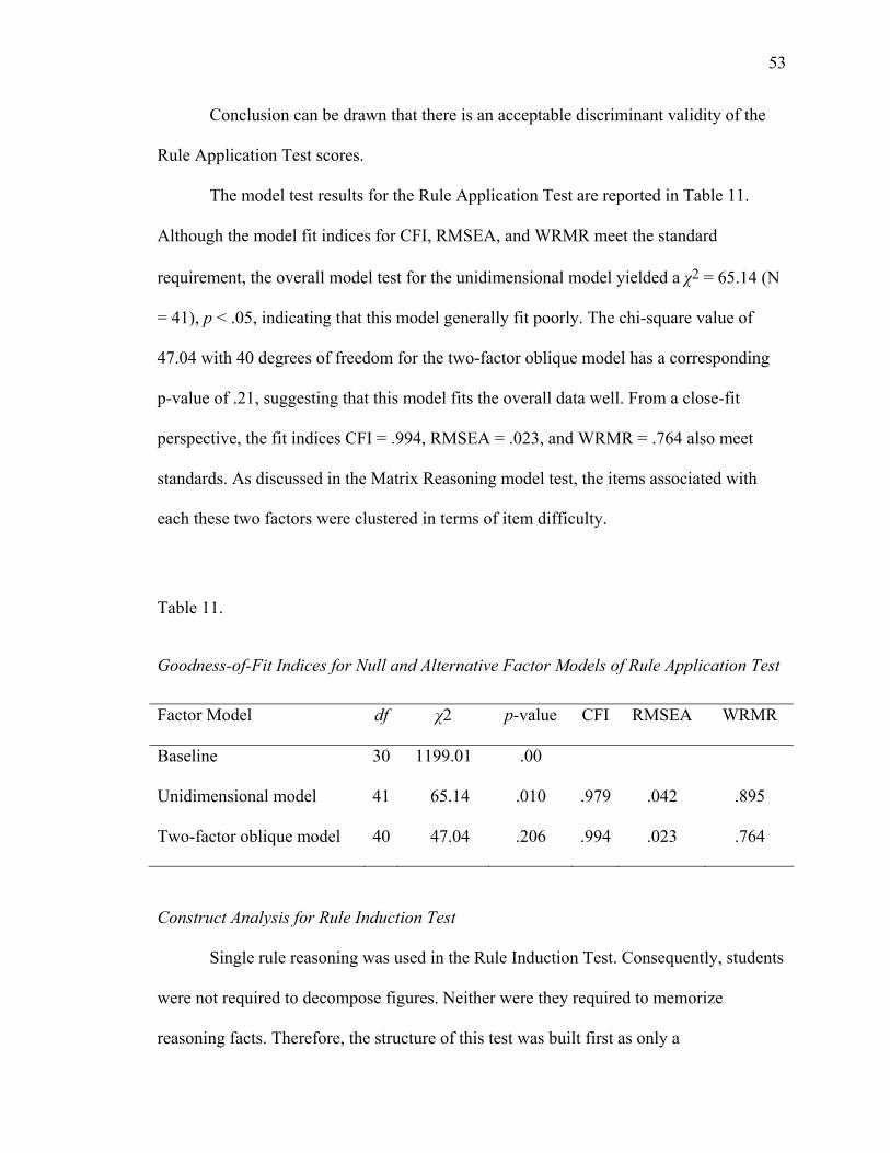
53
Conclusion can be drawn that there is an acceptable discriminant validity of the
Rule Application Test scores.
The model test results for the Rule Application Test are reported in Table 11.
Although the model fit indices for CFI, RMSEA, and WRMR meet the standard
requirement, the overall model test for the unidimensional model yielded a χ2 = 65.14 (N
= 41), p < .05, indicating that this model generally fit poorly. The chi-square value of
47.04 with 40 degrees of freedom for the two-factor oblique model has a corresponding
p-value of .21, suggesting that this model fits the overall data well. From a close-fit
perspective, the fit indices CFI = .994, RMSEA = .023, and WRMR = .764 also meet
standards. As discussed in the Matrix Reasoning model test, the items associated with
each these two factors were clustered in terms of item difficulty.
Table 11.
Goodness-of-Fit Indices for Null and Alternative Factor Models of Rule Application Test
Factor Model df χ2 p-value CFI RMSEA WRMR
Baseline 30 1199.01 .00
Unidimensional model 41 65.14 .010 .979 .042 .895
Two-factor oblique model 40 47.04 .206 .994 .023 .764
Construct Analysis for Rule Induction Test
Single rule reasoning was used in the Rule Induction Test. Consequently, students
were not required to decompose figures. Neither were they required to memorize
reasoning facts. Therefore, the structure of this test was built first as only a

54
unidimensional model. As shown in Table 12, the chi-square value of 10.93 which was
evaluated with four degrees of freedom yielded a corresponding p-value of .28. This p-
value is too high to reject the null of a good fit. Corroborating evidence is provided by
CFI and RMSEA fit statistics. The fit indices for the three statistics are .995, .025
and .062, respectively which all meet the standard requirement. Generally speaking, the
unidimensional model fits the data in an acceptable manner. Therefore, no further model
was estimated for construct analysis of the Rule Induction Test.
Table 12.
Goodness-of-Fit Indices for Null and Alternative Factor Models of Rule Induction Test
Factor Model df χ2 p-value CFI RMSEA WRMR
Baseline model 15 397.13 .000
Unidimensional model 9 10.93 .280 .995 .025 —
Standardized factor coefficients of the item loadings on the factor are presented in
Table 13. All of the coefficients are significant at .01 levels, showing good convergent
validity in the test scores.
Construct Analysis for Figure Detection Test
A Figure Detection Test was used to assess students’ visual spatial ability. In this
test, students were asked to segregate simple pictures embedded in a complex visual
configuration. Since no argument was found in the literature about the dimensionality of
Figure Detection Test, we hypothesized that this test is a unidimensional visual spatial

55
ability test. The model test results for the unidimensional analysis are reported in Table
14.
As can be seen from Table 14, the chi-square obtained for the unidimensional
model yielded a value of 1.14 with two degrees of freedom. The p-value for this test
is .56, indicating an adequate fit of the data. The CFI value is 1.00, which is above the
standard of .95; the values for RMSEA are not available. On the whole, the fit indices
suggest very good model fit.
Table 13.
Standardized Coefficients of Rule Application Items under the Same Factor
Items Coefficients
1 .83**
2 .87**
3 .83**
4 .78**
5 .79**
6 .65**
**p < .001
Table 14.
Goodness-of-Fit Indices for Null and Alternative Factor Models of Figure Detection Test
Factor Model df χ2 p-value CFI RMSEA WRMR
Baseline model 6 28.91 .000
Unidimensional model 2 1.14 .563 1.000 — —

56
Standardized factor coefficients of each item were significant at .01 levels (see
Table 15). However, the standardized item loadings on this factor were relatively low,
indicating that the convergent validity of the test scores was not good.
Table 15.
Standardized Coefficients of Figure Detection Items under the Same Factor
Items Coefficients
1 .36**
2 .43**
3 .55**
4 .57**
**p < .001
Construct Analysis for Working Memory Test
Two formats of Short Term Working Memory items were used in the test; namely,
Binary Number Working Memory items and Shape Working Memory items. Two
measurement models were tested for this test; namely, a unidimensional model with the
two formats of items represented by a single factor and a first-order oblique model with
two separate factors. Since a second-order CFA with two first-order factors and one
second-order factor is always under-identified due to the absence of a constraint on the
higher-order loadings, the second-order factor model was not tested here. Table 16 shows
the fit statistics for the models.

57
Table 16.
Goodness-of-Fit Indices for Null and Alternative Factor Models of Working Memory Test
Factor Model df χ2 p-value CFI RMSEA WRMR
Baseline 24 359.813 .000
Unidimensional model 22 51.868 .000 .911 .064 1.144
Two-factor oblique model 21 20.667 .480 1.000 — .726
The results of the unidimensional model do not show a good fit. The chi-square
value of the unidimensional model is 51.86 with 22 degrees of freedom. The low p-value
< .0001 shows that the data did not fit the model well. The two-factor oblique model had
an overall good fit with chi-square value of 20.667 (df = 21) and p = .480. This model
was also found to have excellent goodness-of-fit indices: CFI = 1.000 and WRMR=.726.
Table 17 illustrates the standardized factor coefficients of the Working Memory
test. Convergent validity is shown by the significant loadings of items on the underlying
factors.
The intercorrelation between the factors of Binary and Shape is .59 with standard
error of .04. The confidence interval for this correlation ranges from .51 to .67, which
suggests acceptable discriminant validity for the Working Memory test scores.
Results for Each Research Question
Research Question 1: Which of the Alternative Models is the Most Valid Representation
of the Domain of Matrix Reasoning Problem Solving?
Construct analysis results for each test were applied to prepare for the data used to
conduct the SEM analysis. For tests with multiple factors (e.g., the Matrix Reasoning

58
Table 17.
Standardized Factor Coefficients on Working Memory Test for Each Identified Factor
across Alternative Factor Models
Items Unidimensional Two-factor Oblique Binary
1 .45** .53**
2 .38** .44**
3 .46** .57**
4 .57** .66**
5 .56** .68**
Shape
1 .58** .61**
2 .67** .71**
3 .77** .83**
4 .61** .66**
**p < .001
Test, the Rule Application Test, and the Working Memory Test), scales were created by
adding up items scores that measure a common underlying factor. To increase the
stability of the parameter estimates, a parceling method was applied for tests with only
one dimension (e.g., the Rule Induction Test and Figure Detection Test). Holt (2004)
recommended that binary items can be parceled by combining items with opposite item
difficulties. Since the data in this research are dichotomous, Holt’s suggestion was

59
adopted. For example, In Figure Detection Test, item 1 (mean = .40) and item 4 (mean
= .66) were combined and item 2 (mean = .47) and item 3 (mean = .49) were combined.
There were two parcels for each unidimensional test.
Overall measurement model examination. The first step of the SEM analysis was
to test the measurement model. This measurement model includes five latent variables as
in Figure 8, with 11 variances for measurement errors, 11 factor loadings, and 10 factor
correlations. Because there were at least two indicators for each factor, this model was
treated as identified.
There is adequate evidence that the measurement model is a good fit. Therefore,
the causal model may be tested through SEM modeling. Using the WLSMV estimation
method, the measurement model was tested against the data.
As shown in Table 18, the chi-square test for the overall measurement model fit
produced a value of 41.168 with 34 degree of freedom. The corresponding p-value of the
chi-square test was .186. Goodness-of-fit indices for the measurement model yielded a
CFI of .991, RMSEA of .025, and SRMR of .032. These indices meet the joint criteria of
fitness evaluation, and indicated a reasonable model fit.
Mode comparisons. A key feature of SEM is the ability to explore causal
relationships among latent variables. The hypothesized causal relationships of the latent
variables are demonstrated in Figures 5 to 7. All of the three models were tested using the
ML estimation method. Results of the model testing are shown in Table 18. None of the
three hypothesized models had a reasonable fit with the actual data. Rule application as a
mediator model yielded a chi-square value of 79.382 with 37 degrees of freedom,

60
Figure 8. CFA measurement model of Matrix Reasoning problem solving.
Working Memory
Matrix Reasoning
Figure Detection
Rule Induction
Rule Application
MR1 MR2 MR3
RI1
RI2
RA1
RA2
HF1 HF2 BINARY SHAPE
e1 e2 e3
e11
e10
e4
e5
e9 e8 e7 e6
0.8040.809
0.4370.253
0.155
0.652
0.2990.825
0.433 0.430
0.528 0.691 0.560
0.892
.545
0.6863 0.6930.571 0.245
0.720
0.876
0.721 0.523 0.686
0.204
0.702
0.6400.5060.3190.800
0.233
0.482
1.000
1.000
1.000
1.000
1.000
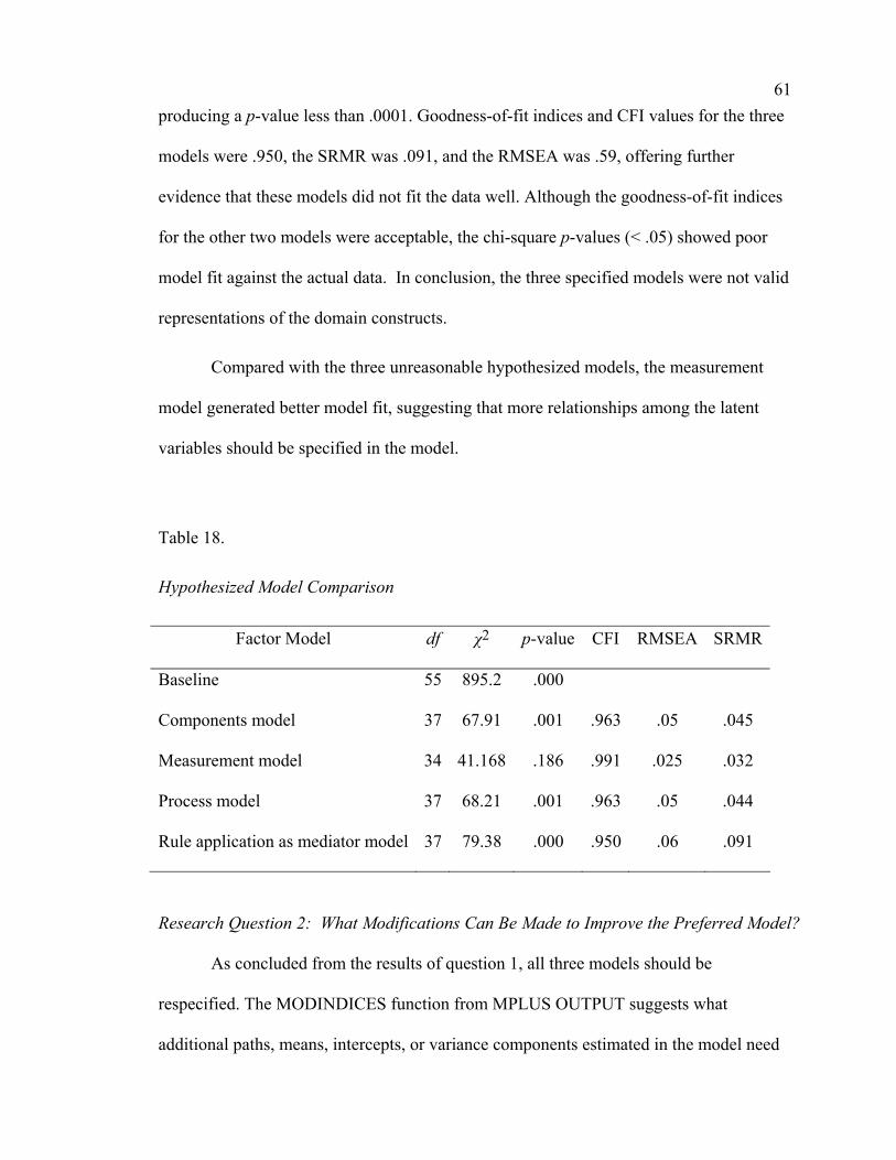
61producing a p-value less than .0001. Goodness-of-fit indices and CFI values for the three
models were .950, the SRMR was .091, and the RMSEA was .59, offering further
evidence that these models did not fit the data well. Although the goodness-of-fit indices
for the other two models were acceptable, the chi-square p-values (< .05) showed poor
model fit against the actual data. In conclusion, the three specified models were not valid
representations of the domain constructs.
Compared with the three unreasonable hypothesized models, the measurement
model generated better model fit, suggesting that more relationships among the latent
variables should be specified in the model.
Table 18.
Hypothesized Model Comparison
Factor Model df χ2 p-value CFI RMSEA SRMR
Baseline 55 895.2 .000
Components model 37 67.91 .001 .963 .05 .045
Measurement model 34 41.168 .186 .991 .025 .032
Process model 37 68.21 .001 .963 .05 .044
Rule application as mediator model 37 79.38 .000 .950 .06 .091
Research Question 2: What Modifications Can Be Made to Improve the Preferred Model?
As concluded from the results of question 1, all three models should be
respecified. The MODINDICES function from MPLUS OUTPUT suggests what
additional paths, means, intercepts, or variance components estimated in the model need

62to be freed in order to improve the model fit. The three models were respecified based on
these suggestions.
Modification suggestions for the latent variables in the components model are
listed in Table 19. The ON STATEMENT suggests that a path should be added from rule
application to matrix reasoning. Since matrix reasoning is an endogenous variable, this
suggestion does not satisfy the theory. Regardless, no further actions were taken to
respecify the component model.
Table 19.
Modification Suggestions from MPLUS for Component Model
Statements M.I. E.P.C. S Std E.P.C. StdYX E.P.C
ON Statement
RAPPLY ON MATRIX 11.13 -5.56 -1.22 -1.22
MODINDICE function suggestions for the process model are listed in Table 20.
Among these suggestions, only the path from figure detection to rule application was
theoretically acceptable. The respecified model was estimated with the same data. It
yielded a chi-square value of 50.718 with a degree of freedom of 36. The corresponding
p- value was .053, which was too high (>.05) to reject the null hypothesis that the model
was a perfect model. Respectively, the goodness-of-fit indices are: CFI = .982, SRMR
= .034 and RMSEA = .035, with a 90% confidence interval from 0 to .056. These index
values are all favorable, indicating that the respecified model is acceptable.

63Table 20.
Modification Suggestions from MPLUS for Process Model
Statements M.I. E.P.C. S Std E.P.C. Std YX E.P.C
ON Statements
RID ON RAPPLY 17.22 -.50 -1.64 -1.64
RID ON MATRIX 27.16 -4.57 -3.32 -3.32
FD ON RAPPLY 17.22 .16 .61 .61
FD ON MATRIX 15.41 1.31 1.13 1.13
RAPPLY ON HID 17.22 1.23 .32 .32
WITH Statements
RAPPLY WITH RID 17.23 -1.05 -.83 -.83
RAPPLY WITH HID 17.22 .33 .31 .31
For the rule application as mediator model, modification suggestions are shown in
Table 21. Besides the paths of Rule induction on working memory and rule induction on
figure detection, adding all other paths in the table would cause the model to have
feedback loops. Since the original model was hypothesized as recursive, all paths which
will lead to reciprocal direct effects would be omitted. Thus, only two paths, from
working memory to rule induction and from figure detection to rule induction, were
added back to the model. Estimation for the respecified model showed adequate model fit:
Chi-square was 43.726 with 35 degrees of freedom, p = .148, CFI = .990, SRMR = .036
and RMSEA = .027, with a 90% confidence interval of 0 to .050.

64Table 21.
Modification Suggestions from MPLUS for the Rule Application as Mediator Model
Statements M.I. E.P.C. S Std E.P.C. StdYX E.P.C
ON Statements
MEMORY ON RID 24.17 .42 .41 .41
MEMORY ON RAPPLY 26.62 .21 .67 .67
MEMORY ON MATRIX 26.21 .86 .59 .59
RID ON MEMORY 24.17 .39 .41 .41
RID ON FD 11.13 .24 .24 .24
RID ON RAPPLY 29.72 .32 1.07 1.07
RID ON MATRIX 30.55 .98 .70 .70
FD ON RID 11.13 .24 .24 .24
FD ON RAPPLY 13.58 .13 .44 .44
FD ON MATRIX 13.68 .43 .31 .31
WITH Statements
RID WITH MEMORY 24.17 .15 .40 .40
FD WITH RID 11.12 .08 .24 .24
Values of selected fit indices for the two acceptable respecified models both met
the goodness-of-fit criteria. To choose the better model, the Akaike information criterion
(AIC) was used. AIC was developed by Hirotsugu Akaike (1974). It can be used to
compare nonhierarchical models from the same data set. AIC indicates model fit and
model parsimony. One of the ways to calculate AIC is AIC = χ 2 +2q, where q is the
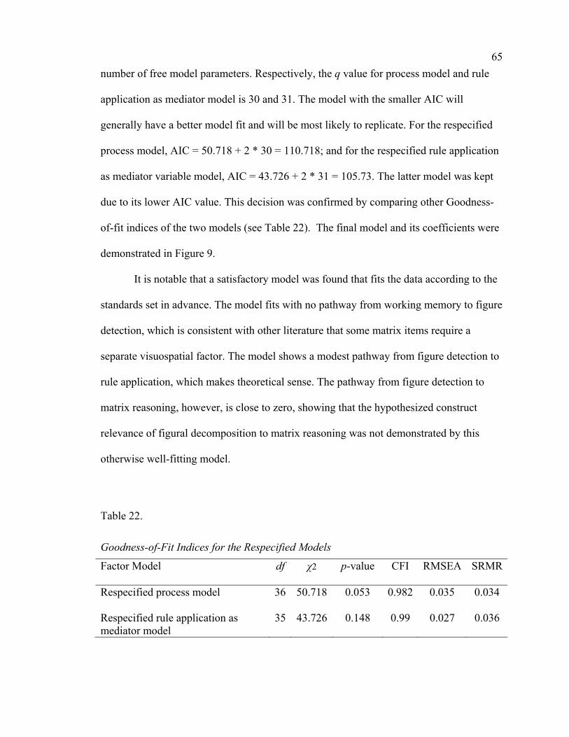
65number of free model parameters. Respectively, the q value for process model and rule
application as mediator model is 30 and 31. The model with the smaller AIC will
generally have a better model fit and will be most likely to replicate. For the respecified
process model, AIC = 50.718 + 2 * 30 = 110.718; and for the respecified rule application
as mediator variable model, AIC = 43.726 + 2 * 31 = 105.73. The latter model was kept
due to its lower AIC value. This decision was confirmed by comparing other Goodness-
of-fit indices of the two models (see Table 22). The final model and its coefficients were
demonstrated in Figure 9.
It is notable that a satisfactory model was found that fits the data according to the
standards set in advance. The model fits with no pathway from working memory to figure
detection, which is consistent with other literature that some matrix items require a
separate visuospatial factor. The model shows a modest pathway from figure detection to
rule application, which makes theoretical sense. The pathway from figure detection to
matrix reasoning, however, is close to zero, showing that the hypothesized construct
relevance of figural decomposition to matrix reasoning was not demonstrated by this
otherwise well-fitting model.
Table 22.
Goodness-of-Fit Indices for the Respecified Models
Factor Model df χ2 p-value CFI RMSEA SRMR
Respecified process model 36 50.718 0.053 0.982 0.035 0.034
Respecified rule application as mediator model
35 43.726 0.148 0.99 0.027 0.036

66
Figure 9. The standardized estimation of the respecified model that empirically fits the
actual data.
Working Memory
Matrix Reasoning
Figure Detection Rule
Induction
Rule Application
.52*
.49*
.02 .36*
.35*
.31*
0.42
.20*
0.23*

67Analysis of the data and reflection on what it means led to some grave concerns
regarding the Figure Detection Test, and thus about the latent variable it is supposed to
measure. These concerns deal with score reliability and convergent validity and should be
discussed in more detail.
The first concern focused on reliability and validity issues. As reported at the
beginning of the results analysis, the Cronbach’s alpha coefficient for the Figure
Detection Test score was .53, which is lower than the acceptable value of .70. The lower
coefficient indicates the inconsistency among the individual items in this scale. Although
the CFA analysis showed a valid unidimensional construct, the relatively low alpha
demonstrated a high degree of random error in item scores. Evidence of convergent
validity was also unsatisfactory for this test because item loadings on the same factor
were relatively low, showing that the items were not theoretically intercorrelated in an
acceptable manner. The low reliability and unsatisfactory convergent validity results of
the Figure Detection Test make its further application in the study unwise.
The second concern about Figure Detection Test relates to its low correlation with
other latent variables. The correlation matrix is reported in Table 23. As shown in the
table, when compared with other correlation coefficients, figure detection has the lowest
correlation of any variable. This suggests the construct irrelevance between figure
detection and other latent variables in the same model.
The third reason for concern about the Figure Detection Test is construct
relevance to the constructs in play within this entire test battery. The Figure Detection
Test was selected for this research to test students’ figure decomposition ability. A

68Table 23.
Correlation Matrix for the Latent Variables in the Model
Working Rule Figure Rule Matrix Memory Induction Detection Application Reasoning
Working Memory 1.00
Rule Induction .43 1.00
Figure Detection .16 .25 1.00
Rule Application .44 .65 .43 1.00
Matrix Reasoning .83 .80 0.30 .81 1.00
well known existing test, Hidden Figure Test, was selected. In this test, the students were
asked to find a picture in a very complicated background that matched one of the listed
pictures in the answer options. A further investigation on each item in this test showed
that student mean score for every item was relatively low, indicating that the items were
difficult for the sample of students who participated in the research. An additional source
of grave concern about the construct match between hidden figures and matrix reasoning
is that not all of the Matrix Reasoning items require students to possess even a moderate
level of figure decomposition ability. More than half of the items had low visual
complexity. Therefore, the overly difficult Figure Detection items were not strongly
relevant to overly easy Matrix Reasoning problems.
Based on the analysis above, a model without the figure detection variable in the
analysis should be examined. The following analyses were redone by dropping the figure
detection variable from the model.

69In the respecified measurement model without the variable of figure detection,
there were only four Latent variables: (a) matrix reasoning, (b) rule application, (c) rule
induction, and (d) working memory. The same estimation method was used as the
measurement model in research question 1. The model testing results are shown in Table
24.
Table 24.
Goodness-of-Fit for Measurement Model with Figure Detection Omitted
Factor Model df χ2 p-value CFI RMSEA SRMR
Baseline 36 799.51 .000
Measurement model 21 27.65 .150 .992 .031 .031
Structural equation model 21 27.65 .150 .992 .031 .031
Measurement model and SEM for this analysis yield the same results. The results
show satisfactory model fit. The chi-square test for the overall measurement model fit
produced a value of 27.65 with 21 degrees of freedom. The corresponding p-value for the
chi-square test was .150. Goodness-of-fit indices yielded a CFI of .992, RMSEA of .031,
and SRMR of .031. Even though the model fit with figure detection was not bad, this one
fits even better. Estimations are given in Figure 10.
Research Question 3: What Are the Significant Direct and Indirect Effects of the Latent
Variables?
Direct and indirect path effects from Figure 10 are reported as follows.

70
Figure 10. The standardized estimation for the respecified model with the figure
detection variable omitted.
Working Memory
Matrix Reasoning
Rule Induction
Rule Application
.52*
.57*
.34*
.36*
0.43*
0.18*

71Direct effects. The direct and indirect effects of the acceptable model respecified
in question 2 are delineated in Table 25. The unstandardized path coefficients, standard
error, ratio of estimation to standard error, and the standardized coefficients are reported
column by column. The unstandardized estimate represents the amount of change in the
outcome variable as a function of a single unit change in the variable causing it. The
estimate divided by the standard error, which indicates a significant effect when it is
larger than 1.96, tests the significance of the parameter estimation. As shown table 25,
besides the paths from figure detection ability to matrix reasoning and from working
memory ability to rule application ability, all other paths in the model have significant
direct effects (ratio values are larger than 1.96).
To examine the relative strengths of association across these latent variables that
are measured using different scales, the standardized coefficients were compared.
Standardized coefficients represent the amount of change in an outcome variable per
standard deviation unit of a predictor variable. For example, the standardized path
coefficient from working memory to matrix reasoning is .52. This means that if working
memory ability increases by one standard deviation from its mean, matrix reasoning
ability would be expected to increase by .52 of its own standard deviations from its own
mean while holding all other relevant connections in the region constant.
Clearly, the relationship of the three latent variables to matrix reasoning in
descending order of magnitude of the standardized coefficients are working memory
ability (.52), rule induction ability (.34), and rule application ability (.36). This finding
demonstrates that the working memory ability is more effective at explaining the shared
variance of matrix reasoning than other latent variables.

72
Table 25.
Results of Standardized Direct and Indirect Effects of the Respecified Model
Effects Estimates S.E. Est./S.E. Std Direct Effects of the Latent Variables
working memory matrix reasoning .38 .09 4.12 .52
rule induction matrix reasoning .27 .08 3.50 .36
rule application matrix reasoning .08 .02 3.14 .34
working memory rule application .62 .30 2.07 .18
rule induction rule application 1.96 .27 7.38 .57
working memory rule induction .42 .10 4.08 .43 Indirect Effects from working memory to matrix reasoning
working memory rule induction matrix reasoning
.11 .04 3.14 .15
working memory rule application matrix reasoning
.05 .02 2.02 .06
working memory rule induction rule application matrix reasoning
.06 .03 2.46 .08
Indirect Effects from rule induction to matrix reasoning
rule induction rule application matrix reasoning
.15 .05 2.82 .20

73Significant effects also exist in the paths from rule induction ability to rule application
ability, from working memory ability to rule application ability, and from working
memory ability to rule induction ability.
Indirect effects. Indirect effects were investigated from the two exogenous
variables working memory and rule induction to the predicted variable of matrix
reasoning. Results from Table 25 show significant indirect effects of working memory
through mediating variables. These three significant paths listed below.
1. working memory rule induction matrix reasoning
2. working memory rule induction rule application matrix reasoning
3. working memory rule induction rule application matrix reasoning
The significant indirect effects partially indicate the flow path of Matrix
Reasoning problem solving. Also, there is a significant indirect path from rule induction
to matrix reasoning through rule application.

74Chapter 5: Conclusion and Discussion
The purpose of this research was to gain a deeper insight into the domain of
matrix reasoning. An attempt was made to develop a valid model to understand the
construct of matrix reasoning. In this SEM model, subabilities involved in solving Matrix
Reasoning tasks were postulated and the relationships among the subabilities were
sufficiently hypothesized. The results explain how typical students in this sample solve
Matrix Reasoning problems. This model provides an explanation supported by empirical
data. The results have implications for designing Matrix Reasoning Tests and instruction.
Before discussing the results, the issue of how the results of SEM are to be
understood must be addressed. As mentioned in the methodology section of this work,
the SEM technique is used to examine hypothesized causal relationships among variables
with a linear equation system and to test whether or not the actual data is consistent with
the model. However, the SEM technique can not prove the causal model. When the
hypothesized model is accepted, the model fit data only support the argument that the
model is a valid representation of the relationships among variables. However, there may
be several alternative models that could fit the data equally well. When the hypothesized
model is rejected, the model is demonstrated as definitely not fitting the data.
Issues Regarding the Figure Detection Test
The Figure Detection Test studied in this research was designed to measure a
hypothesized construct, figural decomposition ability, which refers to find corresponding
figures embedded in complex figures. After reviewing the literature, I found that the
hidden figure task can function as the instrument to measure figure decomposition ability
75because hidden figure task involve figure-ground segregation. This task requires observers
to identify the given simple figures hidden in a complex visual configuration. Hidden figure
tasks also require visual decomposition ability.
However, according to the results of the analysis, figure detection had no
significant direct effect on matrix reasoning, nor did it show any significant indirect
effects through mediator variables. This seems to demonstrate that the figure
decomposition ability does not play a crucial role in matrix reasoning. This result rejected
the hypothesis that figure decomposition ability has a significant effect on matrix
reasoning. This result is consisted with Tsakanikos and Reed’s research (2003). In their
study, Tsakanikos and Reed found that although there was a correlation between the
number of correct responses on Raven’s Progressive Matrices and Hidden Figures Test,
they maintained a substantial amount (> 95%) of non-shared variance. Even so, any
interpretation of this result should consider the following issues.
First, this finding is suspect because the score reliability and validity of the Figure
Detection Test were less than satisfactory. As previously discussed, Cronbach’s alpha
coefficient for the Figure Detection Test was .53, revealing a less than acceptable level of
consistency of the items in this test. In addition, the standardized factor loadings for each
item were too low to demonstrate satisfactory discriminant validity. Also, more than half
of the 14 Matrix Reasoning items did not require figural decomposition ability. The two
reasons listed above are both due to the insufficiently construct-sensitive test design.
Consequently, all results related to the figure detection variable should be interpreted
with caution.

76Second, the results prompted the researcher to reflect on whether or not the
Hidden Figure task was a good format to measure figure decomposition ability. While the
Hidden Figure task requires subjects to visually encode and parse the figures so that one
can find the correct figure in a complicated figural background, it cannot test the process
of finding correspondence elements which requires subjects to ascertain which figure
elements in the three entries in a row are related. Therefore, a conservative conclusion
may be drawn from the results; namely, that whatever construct was measured by the
Figure Detection Test has no direct or indirect effects on whatever constructs are
measured by the Matrix Reasoning Test. This result does not constitute proof that visual
encoding and parsing, appropriately measured, are not important parts of Matrix
Reasoning problems. Also, we must keep in mind that this conclusion is reached based on
the finding that the reliability and validity of Figure Detection Test scores. There is also
evidence that even with its unsatisfactory psychometric properties, figure detection did
relate to rule application ability.
Which tasks in what test format would be effective for assessing the figural
detection construct and its relationship to correspondence finding? This is a question for
future research, informed perhaps by the off-target construct-relevance of part of this
study. Theoretically, correctly testing figure decomposition ability can help future
researchers to answer the remaining questions in this research.
Finding or developing better measures of figural decomposition ability may have
practical benefits worth pursuing. Some learners who can not successfully finish the
Matrix Reasoning tasks may need deeper diagnosis involving figural decomposition
ability and accurate correspondence finding.

77Discussion
As discussed above, figure detection is not a satisfactory variable in this research.
More than half the Matrix Reasoning problems did not require the figure decomposition
ability. Therefore, it was reasonable and appropriate to drop the figure detection variable
from the analysis of the final model.
The three questions addressed in Chapter 4 can be condensed into two to facilitate
discussion. First, is there a valid model representation to demonstrate the relationships
between identified abilities that are applied to solve Matrix Reasoning problems?
Secondly, if there is a valid model representation, what are the significant direct and
indirect relationships between the variables in this model?
In regards to the first question, SEM analysis shows that there is a valid model
which can demonstrate the relationships between latent variables. However, this valid
model is not one of the three hypothesized models. Rather, it is a combination of the three
models. In the first hypothesized model, working memory was the basic variable. In
addition to its direct effect on matrix reasoning, it also had indirect effects through rule
application and rule induction. However, there was no relationship specified between rule
induction and rule application. The second model was the rule application as the mediator
variable model. In this model, all of the variables had a direct effect on matrix reasoning.
Also, rule induction and working memory had indirect effects on matrix reasoning
through rule application. The third model specified the path of working memory rule
induction rule application matrix reasoning. It also set paths from working memory to
rule induction and rule application. Results show that none of the three models were a
sufficient fit to the data. Paths should be set among all the predicted variables.

78The second question will be answered by examining the relationships among the
variables.
The Relationship between Matrix Reasoning and the Other Three Subabilities
In this study, paths from working memory, rule induction, and rule application to
matrix reasoning ability were defined in the model. All three paths showed significant
effects. The relative strength of the relationships can be evaluated by examining the
standardized coefficients. The strongest relationship existed between working memory
and matrix reasoning ability, with a standardized coefficient of .52. The relationships
between matrix reasoning ability and rule induction ability and between matrix reasoning
ability and rule application ability dropped to .36 and .34 respectively. These results
provide evidence that working memory is the most important factor which affects
subjects’ performance in solving Matrix Reasoning problems. This result is consistent
with Lohman’s (2001) study of the relationship between working memory and reasoning
in which he discussed that “although many different processes may be executed in the
solution of a task, individual differences in them may primarily reflect individual
differences in working memory resources” (p. 223). The relationship between working
memory and matrix reasoning will be further examined.
The Path from Working Memory to Matrix Reasoning
As mentioned above, a significant and substantial causal path was found from
working memory to matrix reasoning. The matrix reasoning ability increased .52 of its
own standard deviations from its own mean. Working memory ability increased by one
standard deviation from its mean while holding all other relevant regional connections
constant. Moreover, indirect effects were also established from working memory to
79matrix reasoning. Two variables emerged as significant mediators between working
Memory and matrix reasoning. Subjects who have more working memory ability are
likely to perform better on Rule Induction Test; this in turn increases the likelihood they
will perform better on the Rule Application Test, which leads to an increase in their
scores on the Matrix Reasoning Test. This is an important process. The ability at the
lower order of the path will not only affect performance on solving Matrix reasoning
problems, it will also affect other subablities in the higher order of the path. Although
the majority of the effect is explained by the direct effect, the indirect effects lead to the
interpretation that working memory ability is a component that improves performance on
both rule induction and rule application, and thus on matrix reasoning.
Study Contributions
This study yields a deeper insight into the domain of matrix reasoning. Previous
research has focused more on the item (task) side than on the thinking person side in
attempts to understand the domain of matrix reasoning. Starting from the process of how
a thinking person solves a matrix reasoning problem, this research identified four
subablities which were hypothesized to significantly contribute to matrix problem solving.
By applying the technique of structural equation modeling, variable relationships which
were hypothesized in the models were tested and respecified. The final respecified model
with Figure Detection Test omitted was demonstrated to be a valid representation of the
domain; this model was able to fit well with actual data. This research provided evidence
that working memory ability is the most important resource that can be used to explain
individual differences in Matrix Reasoning problem solving. The rule induction ability
and rule application ability are also significantly and directly connected to matrix

80reasoning. Furthermore, significant indirect effects from working memory to matrix
reasoning through variables of rule induction and rule application indicted that there was
a valid problem solving process path that existed, although the indirect effect was much
smaller than the direct effects. These results provide a different and personal view to the
understanding of the domain of matrix reasoning. By and large, matrix reasoning cannot
be explained by any process independently; it is a combination of working memory, rule
induction, and rule application, and perhaps of other processes not demonstrated in this
study.
This research did not definitively rule out figural decomposition as an important
part of the process. When matrix problems are used with a strong requirement for figural
decomposition ability, it is still possible that more figurally demanding matrix problems
and a valid and reliable figural decomposition test would show an important relationship.
Implications for Training
Inductive reasoning is considered to be the central part of fluid intelligence. Kauer
(2002) stated, “Inductive reasoning enables one to detect regularities, rules, or
generalizations and, conversely, to detect irregularities. This is one way in which we
structure our world” (p. 1). Obviously, improving inductive reasoning ability will allow
for better learning and living in the real world. Studies have shown that fluid ability can
be enhanced with training (e.g., Deeny & Heidrich, 1990; Welko & Johannes, 1997). A
large-scale study by Csapo (1997) has confirmed that inductive reasoning correlates
substantially with school achievement. Training significantly improves performance. For
students, training on inductive reasoning will not only foster their competencies in
intelligence, but also will help them improve their academic learning.

81 Previous training methods for Matrix Reasoning problems included demonstrating
the problem solving process to subjects and then asking them to repeat the process by
using the same strategy (Deeny & Heidrich, 1990). This study provides a potential
method for individualized training. Students may be evaluated by the three tests
developed in this research to diagnose the problems they may encounter as they try to
improve their fluid intelligence. (If the Figure Decomposition ability is counted, then
there are four tests; however, this fourth test requires more development and research.)
Training should ideally be provided based on individual need. After training on
subablities, a problem solving process then will be demonstrated. The learning process is
a circle; diagnosis, training, and evaluation should be combined.
Limitations of the Research
Perhaps the most serious limitation of this research is that the measurement error
from the Figure Detection Test put a brake on our theoretical interpretation and empirical
inference. This is especially true for those Matrix Reasoning questions which have
complex figure combinations. It is confirmed that figure complexity was an important
resource to explain item difficulty differences. Figure decomposition ability therefore
should play an important role in solving Matrix Reasoning problems. Unfortunately, our
Figure Detection Test was not able to provide strong evidence to either reject or accept
this hypothesis.
An issue worthy of consideration is that the Figure Detection Test does not solely
test the Figure Decomposition ability. We were not able to find an appropriate task
format to test the ability of both parsing complex figures and finding corresponding
elements. Also, as shown from the research, typical hidden figure tasks proved to be an

82unsatisfactory task format to test the ability of parsing figures. These limitations
prevented the further understanding of how the figure decomposition construct should
affect matrix reasoning problem solving.
Another limitation of this study is related to external validity. Although the two
schools that participated in this research were randomly selected, they cannot represent
the entire population of either city or rural area. The homogeneity of the sample also
brought further potential limitations to generalizability. Our samples were groups of
students of ages 13 to 15 solely of Chinese nationality. Similar findings and results may
not be guaranteed from a sample more diverse with regard to age or ethnic identity.
Future Research
A continued discussion of the limitations of this research, future research, and
data collection efforts will require refinements in current theories; a number of practical
and theoretical questions will be addressed.
Theoretically, future research should further explore whether a valid test is
available to measure figure decomposition ability. Results from the present research
showed that the Hidden Figures Test can not measure figure decomposition appropriately.
In addition to figural recognition, figure decomposition ability also requires the ability to
find correspondence elements from these figures. A valid Rule Decomposition Ability
Test should measure these two components. Furthermore, if such a valid test exists, how
would the new model including this test differ from the one estimated in this research?
The sample in this research consisted of students from China between the ages of
12 to 15 inclusively. How would the model change to if responses from a larger and more

83diverse sample were investigated? Would a different model fit better for other age levels
or cultural groups? These questions need to be investigated in future studies.
Future research on practical considerations could include the following.
1. How well do the tests developed in this research function when used for
diagnostic and training purposes?
2. Would training in matrix reasoning that focused on using the subability tests
developed in this study be more or less effective than using the training method
consisting of demonstrating the problem solving procedure, as done in previous
research?

84References
Adcock, C. (1948). A re-analysis of Slater’s spatial judgment research. Occupational
Psychology, 22, 213–216.
Alderton, D.L. & Larson, G.E. (1990). Dimensionality of Raven's Advanced Progressive
Matrices items. Educational and Psychological Measurement, 50, 887-900.
Anderson, J.C., & Gerbing, D.W. (1988). Structural equation modeling in practice: A
review and recommended two-step approach. Psychological Bulletin, 103, 411–
423.
Arendasy, M. (2005). Automatic Generation of Rasch-Calibrated Items: Figural Matrices
Test GEOM and Endless-Loops Test E-super(c). International Journal of Testing,
5(3), 197-224.
Arthur, W., & Woehr, D. J. (1993). A confirmatory factor analytic study examining the
dimensionality of the Raven’s Advanced Progressive Matrices. Educational and
Psychological Measurement, 53, 471–497.
Babcock, R. L. (1994). Analysis of adult age differences on the Raven’s Advanced
Progressive Matrices test. Psychology and Aging, 9, 303–314.
Banks, C. (1949). Factor analysis of assessments for army recruits. British Journal of
Psychology. Statistical Section, 2, 76–89.
Belmont, J.M., Butterfield, E.C. (1971). Learning strategies as determinants of memory
deficiencies. Cognitive Psychology, 2, 411-420.
Buehner, M., Krumm, S., & Pick, M. (2005). Reasoning=working memory≠attention.
Intelligence, 33, 251–272.
85Bunderson, C. V. (2000, April). Design experiments, design science, and the philosophy
of measured realism: Philosophical foundations of design experiments.
Symposium session at the annual meeting of the American Educational Research
Association, New Orleans, LA.
Bunderson, C. V. (2002, April). How to build a domain theory: On the validity
centered design of construct-linked scales of learning and growth. Paper
presented at the International Objective Measurement Workshop, New Orleans.
Bunderson, C. V. (2003). How to build a domain theory: On the validity centered design
of construct-linked scales of learning and growth. In M. Wilson (Ed). Objective
Measurement: Theory into Practice, Ablex Publishing Co.
Bunderson, C. V., & Newby, V. (2003). The role of design experiments and invariant
measurement scales in the development of domain theories. In Wilson, M. Ed.
Objective Measurement: Theory into Practice, Ablex Publishing Co.
Baddeley A. (1992). Working Memory. Science, 255, 556-559.
Burke, H. R. (1958). Raven’s progressive matrices: A review and critical evaluation.
Journal of Genetic Psychology, 93, 199–228.
Carpenter, P. A., Just, M. A., & Schell, P. (1990). What one intelligence test measures: A
theoretical account of the processing in the Raven Progressive Matrices test.
Psychological Review, 97, 404-431.
Carroll, J.B. & Maxwell, S.E. (1979). Individual differences in cognitive abilities. Annual
Review of Psychology, 30, 603-640.
Colom, R., & Garcia-Lopez, O. (2002). Sex differences in fluid intelligence among high
school graduates. Personality and Individual Differences, 32, 445–451.

86DeShon, R. P., Chan, D., & Weissbein, D. A. (1995). Verbal overshadowing effects on
Raven’s Advanced Progressive Matrices:Evidence for multidimensional
performance determinants. Intelligence, 21, 135–155.
Dillon, R. F., Pohlmann, J. T., & Lohman, D. F. (1981). A factor analysis of Raven’s
advanced progressive matrices freed of difficulty factors. Educational and
Psychological Measurement, 41, 1295–1302.
Engle, R. W., & Kane, M. J. (2004). Executive attention, working memory capacity, and
a two-factor theory of cognitive control. In B. Ross (Ed.), The psychology of
learning and motivation (pp. 145–199). New York: Academic Press.
Embretson, S. E. (1998). A cognitive design system approach to generating valid tests:
Application to abstract reasoning. Psychological Methods, 3, 380-396.
Embretson, S. E. (2002). Generating abstract reasoning items with cognitive theory. In S.
H. Irvine & P. C. Kyllonen (Eds.), Item generation for test development (pp. 219-
250). Mahwah, NJ: Lawrence Erlbaum Associates, Inc.
Embretson, S.E. (1995). A measurement model for linking individual learning to
processes and knowledge: Application to mathematical reasoning. Journal of
Educational Measurement, 32, 277-294.
Emmett, W. G. (1949). Evidence of a space factor at 11+ and earlier. British Journal of
Statistical Psychology, 2, 3–16.
Gabriel, K. R. (1954). The simplex structure of the progressive matrices test. British
Journal of Statistical Psychology, 2, 3–16.
Gustaffon, J.E. 1984. A unifying model for the structure of intellectual abilities.
Intelligence, 8, 179-203.

87Gustaffson, J. (1988). Hierarchical models of individual differences in cognitive abilities.
In R. J. Sternberg (Ed.), Advances in the Psychology of Human Intelligence, vol. 4
(pp. 35–72). New Jersey: Laurence Erlbaum Associate.
Gorsuch R. L. (1983). Factor Analysis. Hillsdale, NJ: Lawrence Erlbaum. Orig. ed. 1974.
Cited with respect to difficulty factors in use of dichotomous and categorical data.
Green, K. E., & Kluever, R. C. (2001). Components of item difficulty of Raven’s
matrices. Journal of. General Psychology, 119, 189-199.
Hattie, J. (1985). Methodology review: Assessing unidimensionality of tests and items.
Applied Psychological Measurement, 9, 139-164
Hertzog, C., & Carter, L. (1988). Sex differences in the structure of intelligence: A
confirmatory factor analysis. Intelligence, 6, 287–304.
Holt, J.K. (2004, October). Item Parceling in Structural Equation Models for Optimum
Solutions. Paper presented at the 2004 Annual Meeting of the Mid-Western
Educational Research Association, Columbus, OH.
Hornke, L. F.& Habon, M.W.(1986). Rule-based item bank construction and evaluation
within the linear logistic framework. Applied Psychological Measurement, 10,
[Special issue: Test item banking]. 369-380.
Hunt, E. (1974). Quote the Raven? Nevermore. In Gregg L.W.: Knowledge and cognition.
Oxford, England: Lawrence Erlbaum.
Jacobs, P.I.& Vandeventer, M. (1972). Evaluating the teaching of intelligence.
Educational and Psychological Measurement, 32, 235-248.
Jensen, A. R. (1998). The g Factor. Westport, CT7 Praeger.

88Jurden, F. H. (1995). Individual differences in working memory and complex cognition.
Journal of Educational Psychology, 87, 93–102.
Kane, M.J., Hambrick, D.Z., Tuholski, S.W., Wilhelm, O., Payne, T.W., Engle, R.W.
(2004). The Generality of Working Memory Capacity: A Latent-Variable
Approachcto Verbal and Visuospatial Memory Span and Reasoning. Journal of
Experimental Psychology: General. 133, 189–217.
Klauer, K. J., Willmes, K., & Phye, G. D. (2002). Inducing inductive reasoning: Does it
transfer to fluid intelligence? Contemporary Educational Psychology, 27, 1-25.
Kyllonen, P. C., & Christal, R. E. (1990). Reasoning ability is (little more than) working
memory capacity. Intelligence, 14, 389-433.
Kyllonen, P. C. (1996). Is working memory capacity Spearman's g? In I. Dennis, & P.
Tapsfield (Eds.), Human abilities: their nature and measurement. Mawhah, NJ:
Lawrence Erlbaum Associates.
Lim, T. K. (1994). Gender-related differences in intelligence: Application of
confirmatory factor analysis. Intelligence, 19, 179–192.
Lohman, D.F. (2001). Fluid intelligence, inductive reasoning, and working memory:
Where the theory of multiple intelligences falls short. In N. Colangelo & S.G.
Assouline (Eds.), Talent development IV: Proceedings from the 1998 Henry B.
and Jocelyn Wallace National Research Symposium on Talent Development (pp.
219-227). Scottsdale, AZ: Great Potential Press.
Lynn, R., Allik. J., Irwing, P.(2004). Sex differences on three factors identified in
Raven's Standard Progressive Matrices. Intelligence, 32, 411-424.

89Mack, A., Tang, B., Tuma, R., Kalm, S., & Rock, I. (1992). Perceptual organization and
attention. Cognitive Psychology, 24, 475-501.
Marshalek, B., Lohman, D. F., & Snow, R. E. (1983). The complexity continuum in the
radex and hierarchical models of intelligence. Intelligence,7, 107-127.
McDonald, R.P. (1981). The dimensionality of tests and items. British Journal of
Mathematical and Statistical Psychology, 34, 100-117.
McKenna, F.P. (1984). Measures of field independence: Cognitive style or cognitive
ability? Journal of Personality and Social Psychology, 47, 593-603.
McShane, J. (1991). Cognitive development: An information processing approach.
Cambridge, MA, US: Basil Blackwell, Inc.
Messick, &Samuel. (1995). Validity of psychological assessment: Validation of
inferences from persons' responses and performances as scientific inquiry into
score meaning. American Psychologist, 50, 741-749.
Mulholland, T. M., Pellegrino, J. W, & Glaser, R. (1980). Components of geometric
analogy solution. Cognitive Psychology, 12, 252-284.
Muthen, L. & Muthen, B. (2003). MPLUS 3.0 User’s Guide. Los Angeles, CA: Muthen
& Muthen.
Nunnally, J.C., and Bernstein, I.H. (1994). Psychometric theory (3rd ed.) New York;
McGraw-Hill,
Oberauer, K., Suß, H. M., Schulze, R., Wilhelm, O., & Wittmann, W. W. (2000).
Working memory capacity—facets of a cognitive ability construct. Personality
and Individual Differences, 29, 1017–1045.

90Primi, R.(2002). Complexity of geometric inductive reasoning tasks: Contribution to the
understanding of fluid intelligence. Intelligence, 30, 41-70.
Raven, J., Raven, J. C., & Court, J. H. (2000). Standard progressive matrices. Oxford
Psychology Press.
Rost, D.H., & Gebert, A. (1980). On the problem of factor-interpretation in Raven's
Colored Progressive Matrices: Psychological facts or statistical artefacts? Journal
of Individual Differences, 1, 255-273.
Spearman, C. (1904). 'General intelligence,' objectively determined and measured.
American Journal of Psychology, 15, 201-293.
Spearman, C. E. (1946). Theory of the general factor. British Journal of Psychology, 36,
117–131.
Sternberg, R. J. (1986). Toward a unified theory of human reasoning. Intelligence, 10,
281-314.
Tsakanikos, E., & Reed, P. (2003). Visuo-spatial processing and dimensions of
schizotypy: figure-ground segregation as a function of psychotic-like features.
Personality and Individual Differences, 35, 703-712.
Van der Ven, A.H.G.S., & Ellis, J. L. (2000). A Rasch analysis of Raven’s standard
progressive matrices. Personality and Individual Differences, 29, 45–64.
Verguts, T., De Boeck, P., & Maris, E. (1999). Generation speed in Raven’s Progressive
Matrices Test. Intelligence, 27, 329–345.
Yu, C.Y. (2002). Evaluating cutoff criteria of model fit indices for latent variable models
with binary and continuous outcomes. Unpublished doctoral dissertation,
University of California at Los Angeles.

91
Appendix A
Informed Consent Form for Focus Group Participants

92Participants
Informed Consent Form (For principals and teachers)
Introduction This research is being conducted by Kairong Wang under the help of Dr. Richard Sudweeks. Kairong Wang is a graduate doctoral student in Department of Instructional Psychology and Technology of Brigham Young University. The purpose of this research is to investigate how people solve the Matrix Inductive Reasoning problems. Your students are invited to participate in this study. Procedure The students in your school from grade 6 to grade 8 will invited to complete a test online. The test is used to assess general intelligence. It includes five parts. Individually, they are Working Memory test, Rule Induction test, Rule Application test, Hidden Figure test, and Matrix Inductive Reasoning test. The test consists of 46 items and will take approximately 45 minutes. Risk/Benefits There are minimal risks for participation in this study. However, the students may feel frustrated when they are not able to complete some of the items. The benefits to the subjects will be that they have a chance to have a brain exercise. It is hoped that through the students response researcher will be able to learn more about the structure of matrix reasoning ability. It will also bring ideas about how to help the students to improve their reasoning ability. Confidentiality The test is online. Students’ response will be saved in the database directly. Other than those who directly involved with the research, nobody else will be able to access the data. The students’ identities such as name, date of birth, school achievement are not required. The results will only be reported as group data with no identifying information. Compensation Compensation to the students will be the report of results from this research. Further help will be provided under the class teachers’ request. Participation Participation in this research is voluntary. You and the students have the right to withdraw at anytime or refuse to participate for any reason without penalty and without affecting their school standing.. Questions about the Research If you have any questions regarding this study, please contact Kairong Wang at 1-858-566-6475, [email protected] or Professor Richard Sudweeks, (801) 422-7078, [email protected] .

93Questions about your Rights as Research Participants
1. If you have any questions regarding the rights as a participant in this research project, please contact the ORCA office in Brigham Young University. Christopher Dromey, PhD, IRB Chair; 422-6461; 133 LRB; [email protected] .
I have read, understood, and received a copy of the abvove consent and desire of my own free will to participate in this study. Signature: __________________________ Date: __________________________ School: __________________________

94Participants
Informed Consent Form (For students or parents)
Introduction This research is being conducted by Kairong Wang under the help of Dr. Richard Sudweeks. Kairong Wang is a graduate doctoral student in Department of Instructional Psychology and Technology of Brigham Young University. The purpose of this research is to investigate how people solve the Matrix Inductive Reasoning problems. Your students are invited to participate in this study. Procedure You will be invited to complete a test online. The test is used to assess general intelligence. It includes five parts. Individually, they are Working Memory test, Rule Induction test, Rule Application test, Hidden Fgure test, and Matrix Inductive Reasoning test. The test consists of 46 items and will take approximately 45 minutes. Risk/Benefits There are minimal risks for participation in this study. However, the students may feel frustrated when they are not able to complete some of the items. The benefits to the subjects will be that they have a chance to have a brain exercise. It is hoped that through the students response researcher will be able to learn more about the structure of matrix reasoning ability. It will also bring ideas about how to help the students to improve their reasoning ability. Confidentiality The test is online. Your response will be saved in the database directly. Other than those who directly involved with the research, nobody else will be able to access the data. Your identities such as name, date of birth, school achievement are not required. The results will only be reported as group data with no identifying information. Compensation Compensation will be the report of results from this research. Further help will be provided your request. Participation Participation in this research is voluntary. You have the right to withdraw at anytime or refuse to participate for any reason without penalty and without affecting their school standing.. Questions about the Research If you have any questions regarding this study, please contact Kairong Wang at 1-858-566-6475, [email protected] or Professor Richard Sudweeks, (801) 422-7078, [email protected] .

95Questions about your Rights as Research Participants If you have any questions regarding the rights as a participant in this research project, please contact the ORCA office in Brigham Young University. Christopher Dromey, PhD, IRB Chair; 422-6461; 133 LRB; [email protected] . I have read, understood, and received a copy of the abvove consent and desire of my own free will to participate in this study. Signature: __________________________ Date: __________________________

96
Letter of Statement from Principal This is a letter to state that as a principal of Wangjing Middle School in Beijing, I have the legal guardianship of the students on participating in educational research while they are in the school. I have read, understood, signed and received a copy of the consent form of the study from the researcher. The research of “Exploring the Domain of Geometric Inductive Reasoning Problems: A Structural Equation Modeling Analysis” by Kairong Wang is approved to be administrated in our school. 兹证明作为望京中学的校长, 我对我校学生参加在校教育科研有合法的监护权. 我校已经审查并通过王凯荣在我校进行“Exploring the Domain of Geometric Inductive Reasoning Problems: A Structural Equation Modeling Analysis”的研究申请. 签名: __________________________ 时间 __________________________ 学校 __________________________

97Appendix B
Statistics for Each Item in the Tests
Tests
Items Mean Sd
Item-total Correlation Coffiecient
Alpha if Item Deleted
Matrix Reasoning Test
1 .84 .36
.45 0.84
2 .92 .28 .62 0.83 3 .84 .37 .47 0.84 4 .90 .31 .63 0.83 5 .41 .49 .56 0.83 6 .82 .39 .42 0.84 7 .72 .45 .47 .84 8 .70 .46 .62 .83 9 .74 .44 .62 .83 10 .74 .44 .46 .84 11 .42 .49 .35 .85 12 .24 .42 .23 .85 13 .23 .42 .66 .83 14 .49 .50 .44 .84 Rule 1 .60 .49 .36 .88 Application 2 .72 .45 .70 .86 Test 3 .43 .50 .48 .87 4 .42 .49 .45 .87 5 .67 .47 .69 .86 6 .44 .50 .41 .88 7 .69 .47 .74 .86 8 .69 .47 .69 .86 9 .57 .50 .85 .85 10 .33 .47 .83 .85 11 .33 .47 .24 .88 12 .23 .42 .42 .87 Rule Induction 1 .78 .41 .75 .86 Test 2 .89 .31 .78 .86 3 .85 .35 .75 .86 4 .72 .45 .70 .87 5 .77 .42 .73 .86 6 .86 .35 .55 .89 Figure Detection
1 .40 .49
.30 .25
Test 2 .47 .50 .44 .29 3 .49 .50 .49 .37 4 .66 .47 .40 .37
(Table continues)

98
Table 7 (continued)
Tests
Items Mean Sd
Item-total Correlation Coffiecient
Alpha if Item Deleted
Binary Working
1 .84 .37
43 .67
Memory Test 2 .75 .43 35 .70 3 .73 .44 51 .63 4 .82 .38 49 .65 5 .67 .47 51 .62 Shape Working 1 .66 .47 .34 .63 Memory Test 2 .40 .49 .40 .53 3 .30 .46 .49 .49 4 .27 .44 .40 .55