investigating low voltage ride through capability on wind...
TRANSCRIPT

1
School of Engineering and Energy
ENG460 Engineering Thesis
Investigating Low Voltage Ride Through capability on Wind Farm by using Static
Synchronous Compensator (STATCOM) Application
A report submitted to the School of Engineering and Energy, Murdoch University in partial
fulfilment of the requirements for the degree of Bachelor of Engineering
Submitted: December 2012
Author: Zack Forest
Academic Supervisor: Dr. Greg Crebbin

i
Abstract
As an alternative to traditional fossil fuel extracted energy, wind energy has been acknowledged
as one of the most important sources of renewable energies in the world. This clean and
natural source of energy could be a key to solving the worldwide energy crisis with low
environmental impact.
The increased penetration of wind power into the power grids mean the impact of the wind
turbines on the grid can no longer be ignored. Grid codes these days include the requirement
that the wind turbines have to stay connected when the voltage drops. This is known as the
Low Voltage Ride Through (LVRT) requirement. Tripping wind turbines during any fault event
can have a major effect on the stability of the power system.
A voltage regulation device is needed for stability improvement and power quality improvement
of the overall system. The voltage stability issue can be achieved by using Flexible AC
Transmission System (FACTS) devices with the reactive power compensation required by the
power grid. FACTS devices are widely used for enhancing power system performance,
reducing overall power losses, increasing grid reliability and voltage stability.
This thesis investigates the use of Static Synchronous Compensator (STATCOM) on wind farms
for the purpose of stabilizing the grid voltage after a disturbance. The study focuses on a
fundamental grid operation requirement to maintain a voltage at the point of common coupling
by regulating the voltage.
The simulations were carried out by using DIgSILENT PowerFactory software and attaching
STATCOM model in the wind farm model. The results indicate that the STATCOM can provide
an enhanced performance to the power grid. This is mainly achieved by generating or
absorbing the reactive power to provide grid stability during the fault period. Result comparison
was made with the previous results which were carried out by another student in 2010.

ii
Acknowledgments
I would like to thanks my academic supervisor Dr. Gregory Crebbin for all the help, insight,
positivity and advice over the course of this thesis. I thank Dr Martina Calais for all the
knowledge and support throughout my degree towards completion of this thesis. Thank you to
Dr Jonathan Whale for all the knowledge conveyed through the coursework.
Also I would like thank to all my friends from Murdoch University, School of Engineering and
Energy department for their support and help. I would like to thank all those who have directly
and indirectly supported and helped me towards the completion of my thesis.
Special thanks to my wonderful friend, Nebojsa Vuksun for his support, encouragement and
friendship. Our endless conversations will remain unforgettable.
Finally I would like to thank my family for believing in me and supporting me in every ways.
Their love and concern are my inspiration for completion of this thesis.

iii
Contents
Abstract ......................................................................................................................................................... i
Acknowledgments ....................................................................................................................................... ii
Chapter 1 Introduction ............................................................................................................................... 1
1.1 Introduction ................................................................................................................................. 1
1.2 Objective of the Thesis .................................................................................................................. 1
1.3 Thesis Structure .......................................................................................................................... 2
Chapter 2 Background................................................................................................................................ 3
2.1 Global Wind Energy .................................................................................................................... 3
2.2 Wind Energy in Australia ............................................................................................................ 3
2.3 South West Interconnected System (SWIS) ........................................................................... 4
2.4 Western power technical rules .................................................................................................. 5
2.5 Grid code requirement .................................................................................................................... 6
2.5.1 Wind Turbine Condition ..................................................................................................... 6
2.5.2 Active Power Stipulation During Fault Period ................................................................. 7
2.5.3 Voltage Support Requirement During Disturbance ........................................................ 7
2.5.4 Reactive Power and Voltage Control ................................................................................ 7
2.6 Low Voltage Ride Through Capability (LVRT) ....................................................................... 8
2.7 The need for Reactive Power Compensation Devices .................................................................. 9
Chapter 3 Characteristics of Wind Turbine ........................................................................................... 11
3.1 Wind turbine .............................................................................................................................. 11
3.2 Blade aerodynamics .................................................................................................................. 13
3.3 Power control ............................................................................................................................. 14
3.3.1 Stall control (also known as passive control) ............................................................... 15
3.3.2 Pitch control (Active control) ........................................................................................... 15
3.3.3 Active stall power control................................................................................................. 15
3.4 Speed control ............................................................................................................................. 15
3.4.1 Type A: Fixed speed ......................................................................................................... 15
3.4.2 Type B: Limited variable speed....................................................................................... 16
3.4.3 Type C: Variable speed (Partially scale frequency converter).................................... 16
3.4.4 Type D: Variable speed (full scale frequency converter) ............................................ 16

iv
Chapter 4 Doubly Fed Induction Generator (DFIG) ....................................................................... 17
4.1 Steady State Operation ........................................................................................................ 17
4.2 Power Converters .................................................................................................................. 18
4.2.1 Rotor Side Converter (RSC) ............................................................................................. 19
4.2.2 Grid Side Converter (GSC) ............................................................................................... 19
4.3 Converter Losses ................................................................................................................... 19
4.4 Converter Protection System ............................................................................................... 19
Chapter 5 Impact of Wind turbine on Distribution Network............................................................... 20
5.1 Power Compensation for System Stability ............................................................................ 21
Chapter 6.0 Flexible AC Transmission System ............................................................................... 24
6.1 Introduction ............................................................................................................................... 24
6.2.1 Series compensation ......................................................................................................... 25
6.2.2 Shunt compensation ......................................................................................................... 27
6.2.2.1 Shunt capacitive compensation .................................................................................. 27
6.2.2.2 Shunt inductive compensation .................................................................................... 27
6.2.3 Shunt Compensator Operation ...................................................................................... 28
6.3 Static Synchronous Compensator (STATCOM) ................................................................. 29
6.4. STATCOM Operation ............................................................................................................. 30
Chapter 7 Distribution Network Structure and Simulation in Power Factory ................................... 32
7.1 Distribution Network Structure ............................................................................................... 32
7.2 Power Factory ............................................................................................................................ 33
7.2.1 Distribution Network Structure ....................................................................................... 33
7.2.2 PowerFactory STATCOM Model....................................................................................... 37
7.2.3 Modelling DFIG in PowerFactory..................................................................................... 38
7.3 Transient Analysis in DIgSILENT PowerFactory ............................................................... 39
Chapter 8 Results ...................................................................................................................................... 41
8.1 Testing PowerFactory Simulation ........................................................................................... 41
8.2 Constructed model (A1 Wind Farm)....................................................................................... 42
8.3 Voltage control strategy ......................................................................................................... 42
8.4 STATCOM model on 22kV Busbar ...................................................................................... 44
8.5 STATCOM model on Generator Busbar ................................................................................. 45
Chapter 9 Conclusion and Future work ................................................................................................. 46
9.1 Conclusion ................................................................................................................................. 46
9.2 Future Scope of Work .............................................................................................................. 47
APPENDIX................................................................................................................................................... 48

v
Reference ................................................................................................................................................... 63
List of tables
Table 1: Main power system influences of wind energy integration [21] ........................................ 20
Table 2 : Categories of power flow controller ...................................................................................... 25
Table 3 : Synchronous generator parameter ........................................................................................ 34
Table 4 : Line model parameters ........................................................................................................... 35
Table 5 : Induction motor parameters .................................................................................................. 35
Table 6 : Transformer model parameters ............................................................................................. 36
Table 7 : DC source parameters ............................................................................................................. 37
Table 8 : PWM parameters ...................................................................................................................... 37
Table 9 : Transformer parameters ......................................................................................................... 37
List of figures:
Figure 1 : Global wind power capacity [30] ............................................................................................ 3
Figure 2 : South West Interconnected System Structure ..................................................................... 5
Figure 3 Under voltage ride through capability curve [11] .................................................................. 6
Figure 4 Reactive Power Requirement [12] ............................................................................................ 8
Figure 5 : Low Voltage Ride Through Curve [29] .................................................................................. 9
Figure 6 General Scheme of a Wind Turbine and Energy Conversion [16] ..................................... 11
Figure 7: Wind turbine components [28] .............................................................................................. 12
Figure 8 : Ideal wind turbine power curve[20] .................................................................................... 13
Figure 9 : Wind turbine blade [30] ........................................................................................................ 14
Figure 10 : Equivalent Circuit of Induction Generator [38] ................................................................ 17
Figure 11 Doubly Fed Induction Generator [13] .................................................................................. 18
Figure 12 : Two AC power transmission system [22] ......................................................................... 21
Figure 13 : Phaser diagram [22] ............................................................................................................ 21
Figure 14 :(a) Power angel curve (b) Voltage magnitude diagram[22] .......................................... 23
Figure 15 : Overview of major FACTS device [23] .............................................................................. 24
Figure 16 : (a) Power system with series compensation (b) Phaser diagram (c) Real & series
capacitor reactive power Vs angel characteristics [22] ....................................................................... 27
Figure 17 : (a) Power system with reactive compensator (b) Phasor diagram (c) Power angel
curve characteristic[22] ........................................................................................................................... 29
Figure 18: Simple STATCOM model [27] .............................................................................................. 29
Figure 19 (a) : Capacitive-reactive flow ................................................................................................ 30
Figure 20 : Constructed model [Vpu & MVAr Vs Time] ...................................................................... 42
Figure 21 : Voltage control model [Vpu & MVAr Vs Time] ................................................................. 43
Figure 22: STATCOM model at 22kV Busbar [Vpu & MVAr Vs Time] ............................................... 44
Figure 23: STATCOM model next to Generator Busbar [Vpu & MVAr Vs Time] ............................. 45

1
Chapter 1 Introduction
1.1 Introduction
Australia is one of the richest countries in terms of renewable energy resource compared to
other countries, and wind energy is a leading energy source. Renewable energy in Western
Australia has met 5% of the peak load demand and 60% comes from wind energy [33].
Most of the wind farms are located in isolated areas where the power grid is weak or far from
the power station. The uncontrollable nature of the wind causes voltage fluctuation in induction
wind generators. Hence a voltage regulation device is required to provide a better and stable
power system. Many conventional devices such as transformer tap changer, capacitor banks
and mechanical switched cap have been introduced to solve these quality and stability issues of
the network. However these devices are not yet able to solve voltage and power fluctuations
and can even cause stress on wind turbine components.
A Flexible AC Transmission System (FACTS) is an AC transmission system incorporated with
power electronic device that can regulate voltages in a fast and effective way. The Static
Synchronous Compensator (STATCOM) is part of the FACTS family and its properties will be
studied in this thesis.
1.2 Objective of the Thesis
The wind turbine generator and wind farm that are used in this thesis were modelled by a
previous student, Brendan Fidock, 2010 as part of his research. The previous study was carried
out by using voltage control methods to investigate the network support capability and stability
of the network.
A study of the basic principles of FACTS and STATCOM will be carried out as well as reactive
power compensation of STATCOM. The STATCOM model was constructed by using Power
Factory Version14 and was connected to the A1 Wind Farm (AWF). Transient analyses are
conducted using worst case scenarios.
A STATCOM was installed in two different locations for two separate investigations. They are
known to provide an effective voltage supply to the bus they are connected to. Hence they are
installed as close as possible to the busbar which would requires the support after a fault
occurs. A STATCOM is connected to the point of interconnection (a 22kV Bus bar for this study)
and was able to supply the required reactive power to the system when there were
disturbances.

2
1.3 Thesis Structure
Chapter 2 presents a literature review on the wind energy, the South West Interconnected
System(SWIS), Western Power Technical Rules, grid code requirements, low voltage
ride through capability, doubly fed induction generator, Flexible AC Transmission System
and Static Synchronous Compensators.
Chapter 3 describes how wind energy can be harnessed. It also explains wind turbine operation
including their power control and speed control strategies.
Chapter 4 explains the doubly fed induction generator theories, operation of the type of power
converter it uses and its protection system.
Chapter 5 presents the impact of wind turbine on the distribution network and power
compensation for system stability in detail.
Chapter 6 describes around the Flexible AC Transmission System (FACTS) and their controller
types, and discusses in depth regarding the Static Synchronous Compensator
(STATCOM) and its principles of operation.
Chapter 7 explains how the distribution network structure was set up and method of simulation
using PowerFactory by DIgSILENT, step by step including all the elements that were
used.
Chapter 8 summarises the results of the simulations and compares these with the results of
constructed models and the voltage control method that were done by previous study
Vs the STATCOM model
Chapter 9 concludes the analysis and recommends potential future scope of work that can be
performed to extend the thesis.

3
Chapter 2 Background
2.1 Global Wind Energy
Many countries across the globe are facing a greater challenge of finding a reliable, clean, and
efficient renewable energy source and wind energy has become one of the most attractive
sources, since it is free and relatively easy to harness. Many believe that large scale
implementation of wind energy will greatly reduce global warming.
At the end of 2011, the number of operating wind turbine worldwide had reached a total of
200,000 with a total capacity of 238,351 MW which means a 40.5 GW increase over the
previous year, as shown in Figure 1. In 2010, the world wind energy association stated that
wind power has reached 2.5% of the total worldwide electricity usage. Although the wind
industry was affected by the financial crisis in 2009-2010, wind power market penetration is
expected to reach 3.35% by 2013 and 8% by 2018.
Figure 1 : Global wind power capacity [30]
2.2 Wind Energy in Australia
Wind energy is the fastest growing energy source and Australia has some of the best wind
resources compared to other countries. These resources are primarily located in southern,
southern-eastern coastal, western and southern-western regions. Wind energy was first utilised
for electricity generation in 1994 and has expanded rapidly ever since. Australia is targeting to
reach 20% of total energy by renewable energy by 2020 and up to 80% of the renewable
energy source produced in the South West Interconnected System (SWIS) derives from wind
energy[5].Growth in wind energy in Australia has been over 40% per year since 2004 [6].

4
Key influences in utilising wind energy resources in Australia are the government policies, such
as carbon emission reduction and renewable energy target (RET).
Harnessing wind energy is a proven technology and has been in place for many years. An
increase in the manufacture of wind turbines and competition between the manufacturers, have
led to a cost reductions of wind turbines [7].
However, some limiting factors have also been recognised in the development of wind energy
such as lack of electricity transmission infrastructure to access remote wind resources, the
intermittency and unpredictability of wind energy [8].
2.3 South West Interconnected System (SWIS)
The South West Interconnected System (SWIS) is one of the three main systems that makes up
the Western Australian’s electricity market. It is the primary grid in Western Australia, extending
from Albany in the south all the way up to Kalgoorlie in the east and Kalbarri in the north. The
peak demand is around 3800 MW during the summer period, with a total installed capacity of
just over 4500MW. SWIS is generating 17,500 GWh of electrical energy and has network
coverage of up to 90,000 km of power lines. The State government and VERVE energy own
approximately about 65% of the installed generation capacity and remaining 35% is owned by
the private sector. The majority of the electricity supply comes from natural gas or coal power
generation plants. The largest renewable facilities are 90MW wind farms owned by Alinta near
Geralton, 80MW Emu Downs wind farm and 22MW wind farm owned by Verve energy in Albany
[9,10].

5
Private Electricity Generation Stations - Over 10MW
Western Power Interconnected Electricity Generation Stations
Figure 2 : South West Interconnected System Structure
2.4 Western power technical rules
There are certain technical rules for power generating units that are governed by Western
Power and these are summarised below.
In order to provide a reliable service and stable network by Western Power, SWIS must be able
to endure any kind of disturbance. Except in times of an emergency, the minimum steady state
voltage of the system must not go lower than 90% of the nominal voltage and maximum
steady state voltage of the system must not exceed 110% of the nominal voltage. Transformer
tap changing can be used to maintain steady state voltages however this must follow the step-
change voltage limit underlined in Western Power Technical Rules such as routine switching up
to maximum of 4% and infrequent switching up to +6% and below to -10%. This is to control
the acceptable level of voltage when deviations occur. Extended periods of over voltage events
can lead to a network damage that affects the consumers. Figure 3 shows the level of voltage
and function of time.

6
Figure 3 Under voltage ride through capability curve [11]
The generating unit must stay connected if the condition of the power system at the connection
point is to stay within the acceptable envelope for continuous uninterrupted operation. It is
stated that the generator must stay connected for up to 0.45 seconds in order to let the fault
clear during that period. The voltage has to reach 0 pu at minimum between the time period of
0.45 seconds and 0.8 pu at10.45 seconds of the fault event as shown in Figure 3. Then the
voltage has to reach back up to ±10% of nominal voltage after 10.45 seconds [11].
2.5 Grid code requirement
In earlier days, grid codes were applied to generators to prevent degrading of the system
performance and to be remained disconnected in the event of any disturbance in order to
protect network distribution and wind turbines. However, due to integration of large scale wind
turbines and wind energy becoming a major contributor to electricity generation, an advanced
standard of performance is deemed essential. The main requirements of the grid codes are low
voltage ride through capability for improvement in transient stability of the power system and
reactive capability to support voltage control of the power system. As a result of the codes,
every wind turbine generator is required to have voltage ride through capability.
Four main requirements of grid codes related to wind farm performance in the event of voltage
disturbance are detailed in the following sections [12].
2.5.1 Wind Turbine Condition
Requirement of this grid code condition under that the wind turbine must stay connected is
associated with a Voltage Vs Time profile that varies with different regions or countries. The
profile describes the amount of voltage drop that a wind turbine must be able to withstand over

7
some time interval. The voltage should recover to its normal operating state within this time
frame.
2.5.2 Active Power Stipulation During Fault Period
Grid codes vary between different regions or countries. In the UK and Ireland, grid codes
requirement is that “active power should be provided in proportion to the retained voltage”.
And Danish grid codes state that “if possible, active power should be maintained and reduction
in active power is allowed (within plant design specifications)”. The Spanish grid code however
has much more detailed requirements regarding active and reactive power during disturbances
[12].
2.5.3 Voltage Support Requirement During Disturbance
Not only should the supply stay connected during the time of a fault and recovery periods, but
also voltage support requirements are required by injecting reactive current.
2.5.4 Reactive Power and Voltage Control
Earlier modelled generators were known as fix induction generators which absorbs reactive
power from the network system. Reactive power is compensated by installing shunt capacitors,
but compensation is sometimes limited due to a concern over self-excitation in a situation
where the generator is isolated from the network. Reactive power requirements for several
countries are listed in Figure 4 below.

8
Figure 4 Reactive Power Requirement [12]
2.6 Low Voltage Ride Through Capability (LVRT)
Modern wind farms are usually built on a large scale and play a major role in utility grid. Wind
farms had no major effects on the utility grid in earlier days due to the low penetration of wind
power. Generators were allowed to be disconnected during faults and the loss of power
generation from a small wind farm was not considered as a threat to the overall system.
However the size of wind farms has been increasing, as well as their total electricity production.
Impacts on the power system could be severe if entire wind farms are disconnected because of
faults. Therefore a number of grid codes in different regions or countries include low voltage
ride through (LVRT) capability. LVRT is also known as fault ride through capability, which
means the new generation of wind turbine must be able to withstand the fault during any kind
of disturbance in order to avoid being disconnected from the grid. The LVRT demands the wind
generator to keep the system voltage and frequency stable by injecting reactive and active
power back to the grid. The required fault behaviour of the wind turbine can be summarized as
requirements based on the low voltage ride through curve shown in Figure 4.

9
Figure 5 : Low Voltage Ride Through Curve [29]
The LVRT curve can be divided into 4 areas as below:
Area 1 where the fault has to be clear at tmin and voltage dip must not reach lower
than Vmin and it is where the wind generator must stay connected.
Area-2 where the voltage recovery occurs from Vmin upt to Vrem1 in a range of tmin to
t1 .
Area-3 is the period of where the voltage recovery continue before it reaches Area-4
Area-4 is where the nominal operating voltage occurs.
To summarize the LVRT curve, the system must be disconnected if the voltage enters beyond
the grey area. But the boundary limits will be different depending on the regions or countries.
During a fault event, the wind generator must provide reactive power to the grid as required in
order to keep the power system stable. In simulating this LVRT, the system will run normally for
0.5 seconds before the fault event which will last for 1.15 seconds before the fault will gets
clear[29].
2.7 The need for Reactive Power Compensation Devices
The active power supplied to the grid radically decreases during a fault while the input
mechanical power from the turbine is constant. Hence the generator will accelerate during short
circuit to store the excess energy. The resulted turbine speed has to be lower than the
maximum acceptable speed in order to avoid disconnection. After the fault has cleared the
generator draws large amounts of reactive power to increase the machine slip during the fault
event which can delay the recovery of terminal voltage. If the voltage cannot recover in time
then the machine will accelerate further more until it gets disconnected. This could affect the
stability of the network and should be address carefully. Flexible AC transmission system
(FACTS) devices are known to be effective in providing a more stable network system. Among

10
FACTS devices, Static VAR compensator (SVC) and Static Synchronous Compensator
(STATCOM) utilize the latest power electronic technology to control power and voltage flow.
These devices have very important role to play in aiding stability of interconnected power
systems. STATCOMs are used in long distance transmission and in power substations where
voltage stability is of primary concern. The purpose of this device is to control power flow, to
provide reliability and stability of the distribution network and to improve power quality.

11
Chapter 3 Characteristics of Wind Turbine
3.1 Wind turbine
As shown in Figure 6, a wind turbine is a rotating machine that can converts kinetic energy
from the wind into mechanical energy. This mechanical energy can later be converted into
electricity to supply to the grid as shown in Figure 5. This conversion is mainly done between
the rotor and the generator of the wind turbine.
Figure 6 General Scheme of a Wind Turbine and Energy Conversion [16]
The rotor area of the wind turbine consists of blades and hub. The inflowing wind spins the
blades of the turbine and the hub rotates due to the aerodynamic force. The shaft, itself which
is connected to the rotor and gearbox causes this rotation to convert mechanical energy to
electrical energy.
The major components of a wind turbine are shown in Figure 7.

12
Figure 7: Wind turbine components [28]
Power extracted from wind can be calculated as follow:[39]
Pextracted = ½ ρ ACPmax u31
Where:
ρ = density of the air (kg/m3)
A = rotor swept area (m2 = πR2)
U1 = incoming wind speed (m/s)
CPmax = maximum power coefficient
Extracted power is then converted to electrical power which can be calculated as follow:
P = VI
Where:
P = electrical power in watts
V = voltage in volts
I = current in amps
This power can be drawn at different wind speeds as shown in the ideal power curve of Figure
7. The power curve is divided into partial load zone, where the CPmax (power coefficient) is

13
tracked by controlling the rotational frequency of the generator at a fix blade pitch angle to
maintain CPmax value is constant.
Figure 8 : Ideal wind turbine power curve[20]
The cut-in and cut-out speeds are the range in which a turbine can only operate safely. This is
a range to ensure that the available energy is above the minimum point. Rated power is set by
the manufacturer by taking into account the cost and energy. There are three distinct regions in
the Figure 8 and Region (I) consist of low wind speed. The power at low speeds is below the
rated wind turbine power where the turbine needs to run at maximum efficiency to extract all
the available power. Region (II) is region where it is all about keeping the noise and rotor
torque low. On the other hand, region (III) consists of rated turbine power and high speed
wind, the turbine controls the limit of generating power in this particular region [20].
3.2 Blade aerodynamics
There are different types of aerodynamic control strategies that have been applied in the recent
times. But it is important to look into the blade aerodynamic system to understand it’s control
principles.
There are basically two forces L, known as the lift force is orthogonal to the wind speed acting
on the blade and W, which are the force characteristics on an air foil as shown in Figure 8. The
drag force D, has the same direction as lift force. All of these forces mentioned as above are
quadratic function of the wind speed and they are influenced by the angle of attack (α) and the
shape of the airfoil.[30]

14
Figure 9 : Wind turbine blade [30]
Where :
W : wind speed applying on blade
L : Lift force
D : Drag force
WS : fore wind speed
α : angle of attack
3.3 Power control
Harnessing wind energy by using wind turbines is no longer done by a simple approach due to
the demand in energy and the increased in size of the wind farms in modern day. Due to their
fluctuating power levels, the wind turbine requires an electronic control device to keep the
output power in an acceptable range.
Aerodynamic method known as stall control, pitch control and active stall control are the blade
control methods which apply the basic strategies [18.19].
All the wind turbines are designed with power control strategy and there are different ways to
control the aerodynamic force on the rotor in order to prevent excessive power output, optimise

15
the output and to limit the high mechanical loads. There are three types of control, stall, pitch
and active stall control.
3.3.1 Stall control (also known as passive control)
Stall control is the simplest, most robust and cheapest control system. It uses a simple form of
blades which are connected to the hub at a fixed angle. The rotor is designed such that when
the wind speed exceeds a certain level it causes the rotor to stall. In these stall controlled wind
turbines the blade are slightly twisted to make sure the blades slow down steadily rather than
abruptly when the wind speed reaches to its significant stall rate[19].
3.3.2 Pitch control (Active control)
An electronic controller of this pitch controlled wind turbine senses the output power so that the
blade can turn or pitch as required. When the level of power exceeds its limit, an electronic
signal is generated which turns the blades or pitches the blade out of the wind. When the
power level is low, it will pitch back in order to catch the wind at the best possible angle of
attack of the blade air foil [18].
3.3.3 Active stall power control
This is a combination of stall and pitches control and is used in large wind turbines that are
greater than 1MW rated capacity. At the lower wind speed, the blades are pitched just as in
pitch controlled wind turbines to achieve maximum efficiency. However when the wind turbine
reaches its designated power level, the blades pitched slightly in the opposite direction of pitch
controlled wind turbine. These active stall power controlled wind turbines attain a smooth
limitation of power, without the large inherent power fluctuation of pitch controlled wind
turbines. The advantage of this control concept is its ability to compensate for variation in the
air density. It also facilitates emergency stop and assist start-up of the wind turbines.
3.4 Speed control
Wind turbines can be operated either in fixed speed or variable speed mode.
3.4.1 Type A: Fixed speed
This configuration represents the fixed speed controlled wind turbine. An asynchronous squirrel
cage induction generator (SCIG) is connected to the grid via soft starter & capacitor bank. The
capacitor bank is applied in order to compensate the reactive power which is drawn by the
SCIG. It is the cheapest method and provides the most robust system due to its simple
configuration and a lack of converter.
Some drawbacks of this concept are:

16
Does not support speed control
Requires a stiff grid
Its mechanical construction must be able to support high mechanical stresses caused by
wind gusts[18,19]
3.4.2 Type B: Limited variable speed
Type B is a limited variable speed controlled wind turbine which, uses a wound rotor induction
generator (WRIG). The generator is connected to a transformer in a series with a capacitor
bank to compensate the reactive power and to a soft starter to smooth grid connection. The
unique concept of this system is that it has a rotor resistance that can be controlled by
converter mounted on the rotor shaft. This helps eliminate the requirement of expensive slip
rings. Because of this control system, the slip and output power can be controlled [18, 19].
3.4.3 Type C: Variable speed (Partially scale frequency converter)
This is known as the DFIG concept and applies to variable speed controlled wind turbines with
wound rotor induction generator and frequency converter (partially) on the rotor side of the
circuit. The stator is directly connected to the grid side while a partial-scale power converter
controls the frequency of the rotor. Converters of this concept is to compensate reactive power,
to smoother the grid connection. This converter can have a speed range up to 30-40% of
synchronous generator than the Opti slip concept.[18]
3.4.4 Type D: Variable speed (full scale frequency converter)
This concept is a full variable speed controlled wind turbine with wound rotor synchronous
generator (WRSG), or permanent magnet synchronous generator (PMSG) or Squirrel cage
induction generator (SCIG) connected to the grid via a full scale frequency converter. The
frequency converter performs reactive power compensation and helps smooth the grid
connection. Some of the full variable speed wind turbine system does not need a gear box;
instead they use a use a direct driven multiple generator with a large diameter [19].

17
Chapter 4 Doubly Fed Induction Generator (DFIG)
Doubly-fed induction generators (DFIG) are commonly used to generate electricity in a large
wind turbine due to their many advantages over other types of generators. The continuous
trend towards high penetration of wind power in recent years has demanded that new practices
bet set to provide LVRT capability. The main advantage of using DFIG for wind turbines is their
ability to maintain frequency and amplitude of the output voltage at constant rates regardless
of the wind speed. Hence DFIG can be directly connected to an AC power network. DFIG can
also generate electrical power at lower wind speeds [34, 36].
The downside of DFIG is their requirement of complex power conversion compared to
asynchronous machine and the fact that slips rings of a DFIG require regular maintenance.
Even though synchronous generators have the same advantages as DFIG, the AC-DC/DC-AC
converters in a DFIG are much smaller compared to other synchronous generators in terms of
output power, this is because the DFIG converter can only convert 30% of the nominal
generator output power whereas synchronous generator can convey 100% of the nominal
output power[18.19].
4.1 Steady State Operation
The DFIG is an induction machine with wound rotor where both rotor and stator are connected
to voltage sources. The three phase windings of the rotor are energised with three phase
currents. This rotor will create a magnetic field to interact with the stator magnetic field in order
to develop torque. The magnitude of the torque is solely dependent on both the strength and
angular displacement of the rotor and stator fields. The equivalent circuit of the induction
machine is shown in Figure 9.
Figure 10 : Equivalent Circuit of Induction Generator [38]
On the stator side, there are two components Rs and Ls, which are the resistance of the stator
and the leakage inductance of the phase winding. The leakage inductance models all the flux

18
which is generated by the current from the stator winding that does not cross the air gap of the
machines whilst the magnetising branch Lm models the generation of useful flux in the machine
which pass through the air gap between stator and rotor.
Similar to the stator side, the rotor side also has two components, Lr and Rr, which are rotor
leakage reactance and rotor resistance respectively. The rotor side has an additional Rr(1-s)/s
rotor resistance to generate mechanical power. The rotor and stator side are connected via a
transformer in where the ratio is dependent on the ratio of stator and rotor (1:k) turns and slip
(s). Slip can be calculated as:
Where Ns= synchronous speed
Nr= mechanical speed of rotor
Ns = 60 Fe/p .rpm
P = number of poles pair
Fe = Frequency
Figure 11 Doubly Fed Induction Generator [13]
4.2 Power Converters
The converters are placed in a back to back configuration connecting the rotor circuit and to the
grid as shown in Figure 11. The converters are made up of voltage source inverters equipped
with IGBT which allows a bi-directional power flow. And the R-L filter is connected to the grid
side converter in order to minimize switching harmonics.

19
4.2.1 Rotor Side Converter (RSC)
The rotor side converter (RSC) applies voltage to the rotor winding of the DFIG. The main
purpose of this converter is to control the current from the rotor side so that rotor flux position
is aligned with respect to the stator flux. Once an alignment is achieved, the preferred torque is
developed at the shaft of the machine.
The power rating of the RSC is determined by the reactive power control capability and
maximum slip power. RSC acts as a current controlled voltage source converter. [14]
4.2.2 Grid Side Converter (GSC)
The power rating of the grid side converter (GSC) is determined by the maximum slip as it
usually operates at unity power factor in order to minimize the losses in the converter. The
main objective of the GSC is to control the DC link voltage but the converter can also be used to
support grid reactive power during disturbances and enhance the power quality of the grid.[19]
4.3 Converter Losses
The losses of the rotor side converter and grid side converter can be divided into switching and
conducting losses. The switching losses are caused by the turn on-off losses in transistors which
the conducting losses are caused by the current of the transistors and diodes.
When a crowbar detects excessive voltage or current, short circuiting of the rotor winding
occurs. It is important for the active crowbar to remove the short as quickly as possible in order
to maintain continuous operation. Because of this, the rotor side converter can operate right
after the grid disturbance. In this way it is possible to generate reactive current to inject into
the grid to help recover from the fault [35].
4.4 Converter Protection System
The converter of the system is a set of resistor connected in parallel with the rotor winding to
prevent incidental disturbances. The crowbar protection circuit is set to bypass the rotor side
converter. The active crowbar protection system is connected to the crowbar when it is required
and disabled to resume the doubly fed induction control. A DC chopper can also be connected
in parallel with the DC-link capacitor to control the set limit of the overcharge at times where
the grid has low voltage to protect the IGBTs from overvoltage. It can also be used in fully
rated converter topologies as a protection system for the DC link capacitor [14].

20
Chapter 5 Impact of Wind turbine on Distribution Network
The impact on the distribution network by wind turbines will be discussed in this chapter. The
problems can be broken down into small scale and large scale integration.
Table 1: Main power system influences of wind energy integration [21]
Integration scale Problem Causes
Larg
e s
cale
Sm
all
Sca
le
Steady state voltage rise Wind speed variation
Over current Peaks of wind speed
Protection error action Dynamic operation of wind
turbines
Flicker emission during switching
operation
Switching/Startup operation
generators
Voltage drop In rush current due to switching
operation of generators
Harmonics Power electronic converter
Power system oscillations Inability of the power system
controller to cope with the power
variation from the wind farm and
load
Voltage stability Reactive power limitation and
excessive reactive power demand
from the power system
Large scale wind turbine integration includes all the problems of small scale integration but with
the addition of voltage stability and power quality, which are very important issue that need to
be addressed. The voltage stability issue is related to the restriction of transferring power from
the generator to the grid but broad use of capacitor banks in order to compensate reactive
power can also result in major problems when islanding occurs. [21]
Any kind of disturbance in a large scale wind farms can cause voltage transient instability
because of the reduced capacity in transferring reactive power and the huge draw on the
induction generator right after the fault has been removed.

21
5.1 Power Compensation for System Stability
Figure 11 presents two generators connected by a transmission line as a simplified power flow
diagram. The following analysis assumes Assuming there is no loss in a transmission line.
Figure 12 : Two AC power transmission system [22]
Figure 13 : Phaser diagram [22]
X = reactance of the transmission line
E1∠δ1, E2∠δ2 = Voltage phases for buses 1 & 2 respectively
δ = δ1 – δ2 = Power angle
Current magnitude in the transmission line can be calculated by:
∠δ ∠δ
Active component of the current flow at bus 1 can be calculated by:
Reactive component of the current flow at bus 1 can be calculated by:

22
δ
Thus, reactive and active power at Bus 1 are given by:
δ
δ
∠δ ∠δ
Active component of the current flow at bus 2 can be calculated by:
Reactive component of the current flow at bus 2 can be calculated by:
δ
Thus, reactive and active power at Bus 2 is given by:
δ
δ
From Equation 4.1 - 4.5, it can be seen that reactive power can be controlled by regulating
voltage, power angels and the impedance of the transmission line.

23
Figure 14 :(a) Power angel curve (b) Voltage magnitude diagram[22]
From the power angle curve in Figure 14 (a), it can be seen that active power is at its
maximum value when a power angel δ is 90˚. Voltage magnitude regulation is related to the
compensation of the reactive power flow. The change in voltage magnitude of Bus 1 E1 does
not alter the voltage magnitude of EL like current phase angle is varied. There are two power
compensation models in transmission line [22], which are series compensation and shunt
compensation.

24
Chapter 6.0 Flexible AC Transmission System
6.1 Introduction
The Flexible AC Transmission devices have developed along with the growing capabilities of
power electronic components. Flexible AC Transmission Systems are well known for their higher
controllability in power distribution system by means of applying power electronic devices.
FACTS can be define as “Alternating current transmission system incorporating power
electronic-based and other static controllers to enhance controllability and increase power
transfer capability” .[25] A numbers of new devices are already in the industry. The basic
application of FACTS devices are:
Reactive power compensation
Stability improvement
Power quality improvement
Power flow control
Voltage control
Increase of transmission capability
Power conditioning
Flicker mitigation
Interconnection of renewable and distributed generation and storage
Figure 15 : Overview of major FACTS device [23]

25
Figure 15 describes a number of devices which can be divided into conventional and FACT
devices. The left side shows the conventional devices that build upon fixed or mechanically
switchable components like resistance, inductance or capacity with the addition of a
transformer. Not just FACTS devices but also conventional devices use power electronic
converters or valve to switch with a pattern within a cycle of alternating current. These
additional devices have been in industry for many years. Conventional devices have low losses
due to their low frequency switching.
There are dynamic and static devices on the in FACTS side. The dynamic label applies to all the
fast and controllable devices facilitated by power electronic devices. Static implies that no
moving parts are involved such as the mechanical switches that are used in dynamic controllers
[22, 25].
There are a number of FACTS controllers and most of them can perform both steady and
transient operation. Three categories of power flow controllers can be seen in the following
Table 3.
Table 2 : Categories of power flow controller
Conventional Thyristor Controlled Solid-state
Switched shunt capacitor and
inductor
Static Var Compensator(SVC) Static Synchronous
Compensator (STATCOM)
Switched series capacitors Thyristor Controlled Series
Capacitor (TCSC)
Solid-state Synchronous
Compensator(SSSC)
Tap-changing transformer
Phase Shifter
Thyristor Controller Phase
Shifter Transformer
Solid-State Phase Shifter,
Unified Power Flow
Controller(UPFC)
There are two types of compensation-series compensation & shunt compensation.
6.2.1 Series compensation
There are two main methods used to increase the power output in a transmission lines and one
is to increase the voltage of the transmission line. But it will be expensive to increase the size of
the generator and require additional work. Another method is to control the impedance of the
transmission line, which can be done by adding a capacitor in a series with the power line. This
is also known as series compensation.

26
A two machine power system with series compensation in the transmission line is illustrated in
Figure 16. It is assumed that the transmission line(X) are losses and Vs = Vr = V in Figure 16 .b
The total voltage across the series line inductance can be calculated by Vx =2Vx/2
A series of capacitor compensation controller is connected in the middle of the transmission
line. And phase diagram is shown in figure 16.b.
The total transmission impedance Xtotal with the series capacitive compensation can be express
by:
Xtotal = X – Xc =(1-k)X (6.1); where k is the degree of series compensation
Active power transmitted by the transmission line is given by:
The line current is given by:
The reactive power supplied by the series capacitor can be calculated as by this:
The correlations between power (P), series capacitor reactive power (Qc) and power angle (δ)
are shown in Figure 16.c. It can be seen that the active power increases rapidly as the degree
of series compensation (k). The increase in degree of series compensation (k) also results in
increasing the reactive power supply by series compensator [22].
The drawback of these series compensators is that they require protective devices for the
capacitors and they must be able to bypass the high current when a short circuit occurs. Also
adding a series capacitor to the system establishes a resonant circuit that can oscillate at the
frequency below the synchronous frequency caused by the disturbance.

27
Figure 16 : (a) Power system with series compensation (b) Phaser diagram (c) Real & series capacitor
reactive power Vs angel characteristics [22]
6.2.2 Shunt compensation
FACTS device are connected in parallel with the power system. A shunt controller can be a
variable source, variable impedance or a combination of both. Their principle of the operation is
to inject current in to the power system. There are two types of shunt compensation, shunt
capacitive and shunt inductive [24, 22].
6.2.2.1 Shunt capacitive compensation
The purpose of the shunt capacitive compensation is to maintain the stability of the system by
injecting reactive power along the line. The load current lags when an inductive load is
connected to the transmission line, where the shunt capacitor draws current that leads the
source voltage.
6.2.2.2 Shunt inductive compensation
This method is use to charge the transmission line or where there is high voltage at the
receiving end of the power system. When a low current flows through the transmission line due
to low load or no load, the shunt capacitor will cause voltage amplification. To compensate this,
a shunt inductor can be connected across the line.

28
6.2.3 Shunt Compensator Operation
A two machine power system with shunt compensation in a transmission line is illustrated in
Figure 17 (a). It is assumed that the transmission line(X) are lossless and Vs = Vr =Vm= V in
Figure 17 (b). A shunt compensator is connected in the middle of the transmission line (X)[22].
Active powers inject at each terminal are equal and can be calculated by the equation.
The reactive power generated by shunt compensator is given by:
(
)
The relationship between real power P, reactive power Q and angle δ can be seen in figure 17
(c). It can be concluded that the shunt compensation at the midpoint of the transmission can
increase the power noticeably.

29
Figure 17 : (a) Power system with reactive compensator (b) Phasor diagram (c) Power angel curve
characteristic[22]
6.3 Static Synchronous Compensator (STATCOM)
A STATCOM is a shunt type static synchronous compensator that can inject or absorb reactive
power. It is based on a Voltage Source Converter (VSC) power electronic device. It consists of a
DC voltage source (capacitor), a VSC and a transformer as shown in Figure 18. The capacitor
provides a DC voltage to the VSC where it will be converted into a controllable three phase
voltage with the frequency of the AC power system. [22, 24]
Figure 18: Simple STATCOM model [27]

30
6.4. STATCOM Operation
The operation of the STATCOM illustration can be seen in Figure 19 (a, b).The basic purpose of
the STATCOM is to exchange reactive power within the grid. This can be done by varying the
amplitude of the three phase STATCOM voltages.
When a STATCOM voltage is higher than the grid voltage, the converter generates capacitive-
reactive power to the grid. If the STATCOM voltage is drop lower than grid voltage, the
converter absorbs the inductive-reactive power from the grid. STATCOMs can supply reactive
power directly by controlling the inverter firing angle to improve the system stability [37].
Figure 19 (a) : Capacitive-reactive flow
Figure 18 (b) : Inductive-reactive flow
δ
Where:
V1 = Line to line voltage of Source V1
V2 = Line to line voltage V2
X = Reactance of interconnection transformer and filters

31
= Angel of V1 with respect to V2
The amount of reactive power is given by: [24]

32
Chapter 7 Distribution Network Structure and Simulation in Power
Factory
7.1 Distribution Network Structure
A1 Distribution network
The A1 distribution network structure is directly taken from (Brendan Fidock 2010). No changes
in the distribution network model or parameters were made in this section, so that it is easy to
do comparisons. The model includes external grid, substation, loads, transformers and feeder
lines from the wind farm. The external grid is supplied by three 132/22kV transformers from the
substation. Two of the transformers are running parallel in normal operation mode with another
one as a backup.
Wind farm Feeders
There are two wind farm feeders which connect directly to the substation from the wind farm.
They are 12km long and consist of 240mm2,termitex, and underground copper cables (22kV).
The wind farm is connected to the 22kV busbar of the zone substation through these wind farm
feeders.
Substation loads
These domestic loads are fed by the substation and they are expected to rise due to the
increased of residencies. Maximum load occurs in winter due to the cold climate, which draws
more power, the average peak power is around 40MW and the lowest load was 13MW. But this
analysis will used 40MW for the maximum and 10MW for the minimum as Brendan Fidock,
[2010] assumed.
A1 wind farm
The A1 wind farm included twelve ENERCRON wind turbines but all are lumped into one in the
simulation. The simulation model was directly taken from Brendon Fidock, [2010] study.
External grid model
The external grid represents the transmission network feeding into the A1 zone substation. And
the PowerFactory model can be seen in Appendix.
The model has the ability to specify the fault current that the transmission line can provide
when the fault current occurs. Due to the specification by the Western Power the fault level is

33
326MW when both transmission lines are operating at the grid side. If one of the lines is out of
service then the fault level will be reduce down to 12MVA.
7.2 Power Factory
All the simulations in this thesis were carried out using DIgSILENT PowerFactory version 14.0.
The main reason behind using the PowerFactory is its ability to analyse a large distribution
network, including the following analysis:[1]
balanced and unbalanced system power flow
static and dynamic voltage stability
reliability of the distribution/transmission and generation
7.2.1 Distribution Network Structure
Synchronous Generators
The ( ) button from the drawing toolbox represent a synchronous generator. After
placing the generator to the busbar that are connected then an object is created in a database.
The model can be defined by filling in the information that is given in generator specification
sheet. These are parameters of the generator that require to be filled in:
Rated power
Rated voltage
Sub-transient time constants (Td’,Tq “)
Transient constant (Td’)
Transient reactance (xd”)
Sub transient reactance in per unit value
Sub-transient reactance in per unit vales
Acceleration time constant
Stator resistance
Leakage reactance
The generator can be a predefined model from the PowerFactory library or the user defined
one.

34
Synchronous generator
Table 3 : Synchronous generator parameter
Nominal apparent power 22.73 MVA
Nominal Voltage 415V
Power Factor 0.95 per unit
Load flow
Active power 15MW
Reactive power -4.93MVar
Synchronous reactance’s Xd=2.61pu, Xq=1.57pu
Inertia The acceleration time constant of 4 seconds
PWM
There are two types of PWM in PowerFactory. They are PWM-1 Dc connection and PWM-2 DC
connection. But only PWM-1 DC connection will be used for this simulation. And it can be draw
by selecting button ( ) from the main toolbox and drag them to connect to the terminal.
The user can fill in following information after double clicking on the PWM icon.
( )
Rectifier model
Rated AC voltage 415
Rated DC voltage 560V
Diode/Thyristor converter Diode
Built in transformer Default turn ratio
Inverter model
Rated AC voltage 415V
Rated DC voltage 560V

35
Rated power 37.8 MVA
Modulation Sinusoidal PWM
Control mode
Steady state P-Q control
Transient Vac-phi
Line model
Table 4 : Line model parameters
Rated current 479A
Positive/Negative/Zero sequence resistance 0.161 ohms/km
Positive/Negative/Zero sequence reactance 0.067 ohms/km
Length of the line in kilometres 12 kms
Load
The load in PowerFactory can be selected using this icon ( ) button from the drawing
toolbox and drag them to the terminal to connect. Loads can be edited/add in active and
reactive consumption box respectively.
Induction model (MOTOR)
Table 5 : Induction motor parameters
Rated voltage 22 kV
Input mode Electrical Parameters
Power rating 4000kW (mechanical power)
Nominal frequency 50Hz
Number of Pole pair 1 pole pairs
Connection Delta
Transformer
PowerFactory has many types of transformer such as two winding transformer, two winding
neutral transformer, three winding transformer, boosting transformer and auto transformer.
The transformer can be a predefined type from the library or a user defines type. A user can
obtain a data from the manufacture’s data sheet then can easily choose from the library. But

36
it’s necessary to connect high voltage and low voltage busbars correctly otherwise error
message will appear. The HV/LV sides can be flipped by clicking on “Flip connection” button
which will then reverse the connection between high voltage and low voltage busbar/terminal.
A user defined type of transformer can be used if all the required data can be filled in such as
rated power, rated voltage, short circuit voltage and X/R ratio.
2-winding ( ) 2-winding-N ( )2-winding ( ) Booster Transformer (
) 3-winding ( ) ,Auto Transformer ( )
Transformer model
Table 6 : Transformer model parameters
Rated power 20-24 MVA
Nominal Frequency 50Hz
Rated voltage HV-LV (Depend on where the transformer
was used
There are two type of configuration in PowerFactory model that was used for the network.
Delta –Wye neutral model was use for the connection side of the A1 wind farm to A1
distribution network. And zone substation transformer configuration is Delta-Delta.
Terminals
There are two types of node in PowerFactory such as Busbar and Terminal. The terminal model
act as the busbar and their ability is being able to isolate the network easily. Because of this
function, simulation can be switched on/off as required while carrying out the power flow
analysis. PowerFactory offer many predefined busbar systems. For example, single busbar
systems, single busbar system with tie breaker, double busbar system, and double busbar
system with tie breaker and so on. All of these busbar systems include breakers and dis-
connectors as well. Terminal ( ) was used for this simulation. First draw a terminal on
single line diagram. A pop up dialogue box will appear after double clicking on the terminal. All
the required data can then be filled in the provided box. Please see the procedures in Appendix
.

37
7.2.2 PowerFactory STATCOM Model
DC Source
PowerFactory support five type of shunt impedance such as Shunt C ( ), Shunt RL (
), Shunt RLC ( ), Shunt RLCRp ( ) and shunt RLCCRp ( ). For modelling
the STATCOM shunt C was used. The necessary information for creating Shunt C model is
shown in following table 7.
Table 7 : DC source parameters
Rated Reactive Power 5 MVAr
Rated Voltage 200V
PWM
Table 8 : PWM parameters
Rated Power 5MVA
Rated AC voltage 0.415
Rated DC voltage 0.3
Voltage set point value (p.u) 1.01
Current (p.u) Minimum -1.1,Maximum 1.1
Current(MVAr) Minimum -27.5,Maximum 27.5
Controlled bus Point of Interconnection Busbar (22kV)
Transformer
Table 9 : Transformer parameters
Rated power 25MVA
High voltage/Low Voltage 22-0.415V
The remaining parameters are used the same as the WTG TX (wind turbine transformer)
parameters used in Brendan Fidock’s model.

38
7.2.3 Modelling DFIG in PowerFactory
PowerFactory was used to model and simulate a DFIG model and test the stability analysis of
the large power system. At first the wind turbine model and power system will be simulated for
normal operation without any disturbance. Then a fault will be introduced to see how the DFIG
reacts to the fault and whether the generator meets the grid code requirements.
PWM
The converter used in the wind turbine use a self-commutated PWM circuit; IGBTS are used
because of their capability for higher switching frequencies. The model in DIgSILENT can be
seen in the Appendix.
Inductor
The inductor is use in the DFIG model to smooth the output current of the converter. The
inductor can also be integrated in to the 3-winding transformer. The model in DIgSILENT can
be seen in the Appendix.
Capacitor bank
The capacitor bank is an electrical component that can be used in fixed speed or limited
variable speed wind turbines. The purpose of this device is to supply reactive power to either
the induction generator or to the grid. The system is the combination of shunt capacitors which
can be on/off depending on the reactive power strain. The user can choose their desired device
in DIgSILENT between the different types of shunt elements such as C,R-L or R-L-C. The model
in DIgSILENT can be seen in the Appendix.
3-winding Transformer
DIgSILENT provides two-winding, three-winding transformer models. A three-winding
transformer is used in this DFIG model. The model includes tap changers with voltage, active
power or reactive power control. The model in DIgSILENT can be seen in Appendix.
A DFIG model was originally planned for this investigation. Unfortunately, there was a problem
with the simulation and the program continually crashed before plotting the result. Due to
limited time frame, this study had to stop and the investigation move to the next topic with a
similar project plan.

39
7.3 Transient Analysis in DIgSILENT PowerFactory
The first thing to perform before running a transient simulation is to set up the initial
conditions. To perform the system initialization, the button ( ) has to be selected and a pop
up window appears with several settings already defined. The user can choose the desired
simulation method from the following
RMS value
Instantaneous Values
Network-Representation
Balance, Positive Sequence
Unbalanced, 3-Phase (ABC)
Simulation can then be carried out by selecting ( ) and can also be stopped if required by
selecting ( )
Creating simulation plots
The selection of the signal can be performed by creating a result object for the element which
is required for the selected study, such as Busbar, Generator, Load or Transmission line. For
example if the user wants the instance variable of the Generator for analysis, this can be
achieved through a new result object by selecting the generator and then selecting “ Define
Variable” then set “Sim”. This will create a new result object which is stored in “Study Case\All
Calculations”. The user can edit the result object by clicking this ( ) or selecting “Data
Manager –Study Case – All Calculation” and choose “Edit” for the ideal element. The new
window can be seen in Appendix.
The variables are grouped in to different variable sets such as Bus Results, Signal and
Calculation Parameter. The selected variables are stored in the result object and can be plotted
when a user needed.
The graphs can then be inserted in “Virtual Instrument Panel” where they are stored and can
be displayed when required.

40
The number of graphs on a page can be determined by selecting the button ( ) from the
main tool box. After this selection, variables need to be assigned for plotting which can be done
by double clicking on them. A new window will pop up and the user can double click on the
‘Element” and the entire defined result object can be seen in the list. The user needs to select
the desired object to plot next. Selecting the variable can be done by double clicking on the
‘Variable” column, which will display all the variables of the result object. There are parameters
such as line style, colour and line width which can be adjusted in other column.
Several variables can be added to the same graph by double clicking on the curve number and
by selecting “Append Rows” as shown in the Appendix.
The following editing tools for the graphs can be found in the main graphical toolbox.
They can be used for scaling plot for X-Y axis automatically.
Specific area of the plot can also be adjusted by using button ( ) ( )
Graphs can be edited by using ( )
Extra sub plot can also be added into the existing one by using ( ).

41
Chapter 8 Results
8.1 Testing PowerFactory Simulation
A transient analysis is used to investigate a worst case scenario to test the stability of the
voltage on the A1 wind farm. The A1 wind farm power output is set to 15MW and the peak
load is set to a maximum of 40MW. Both the busbar and the AWF are demanding reactive
active power at this situation. It is assumed that the wind speed and load are constant.
To carry out this analysis, a fault is simulated at 22kV busbar. It is the best location to test
voltage stability of the network and their support capability [32]. According to Western Power
Technical rules, section 2 the circuit breaker clearance time for 33kV or less can take up to only
1.16 seconds .In PowerFactory, the short circuit is set to occur after 0.5 seconds and the fault
will be cleared after 1.66 seconds (i.e the fault will last only 1.16 seconds). The total simulation
time is set to 10 seconds.
The voltage is expected to reach an acceptable range after the disturbance even though
Western Power Technical Rules does not state anything. But the acceptable voltage range is
±10% of the nominal voltage and expected to achieve this within the total simulation time (10
seconds). If the voltage at the 22kV busbar or point of generator connection does not reach to
the acceptable range, then the generator will be disconnected, which is not desirable. The
simulation is first carried out with the constructed model, which was set up by Brendan Fidock
[2010]. A second simulation uses a voltage control model which was also carried out by
Brendan Fidock, and the last simulation is STATCOM model implemented on Point of
Interconnection Bus bar on the A1 Wind Farm. This bus bar was chosen because it is the
connection point before the voltage is stepped up by a transformer at the zone substation.

42
8.2 Constructed model (A1 Wind Farm)
The system was operating at voltage 1.0 per unit before the fault occurs at first. After 0.5
seconds, the simulation set a short circuit on the 22kV bus bar and voltage drop down to 0.25
per unit. The fault is cleared after 1.16 seconds and voltage increase back to 0.8 per unit. The
voltage was in steady state until 6 seconds before the controller of the wind farm changed the
absorbing reactive power into generating mode to bring the voltage back up to 0.9 per unit
which can be seen in Figure 20.
Figure 20 : Constructed model [Vpu, MVAr Vs Time]
8.3 Voltage control strategy
The voltage control strategy was done by changing the constant PQ control of the set point
[15MW and -4.93MVar (0.95 leading)] from the PWM to constant voltage control by setting AC
voltage control set point to 1.0 per unit. By doing this, after the fault has been cleared the
power converter will set its control to reactive power generation mode [32]. The simulation
result is shown in Figure 21.

43
Figure 21 : Voltage control model [Vpu, MVAr Vs Time]
The system was operating at voltage 1.0 per unit before the fault occurs at first. After 0.5
seconds, the simulation set a short circuit on the 22kV bus bar and voltage drops down to 0.1
per unit. The fault is cleared after 1.16 seconds and the voltage increases back to 0.8 per unit.
It is clear that the voltage is still outside the acceptable range which is 0.9 per unit. After 5
seconds, the controller revert the wind farms from absorbing the reactive power into generating
mode, so that AV voltage will reach 1.0 per unit. This is expected to happen quicker with the
actual ENERCON controllers [32] compared to Power Factory simulation.

44
8.4 STATCOM model on 22kV Busbar
Figure 22: STATCOM model at 22kV Busbar [Vpu, MVAr Vs Time]
The STATCOM model is connected on the 22kV busbar (Point of Interconnection) and
simulation was done by following the exact procedure that was used in the first two
simulations. The Figure 22 shows that the voltage drops to only 0.557 per unit after the fault is
cleared. After 2.5 seconds the voltage is in steady state even though it is not in the acceptable
range. But after 4 second the voltage increase back to 0.9 per unit in less than 6 seconds. As
previously explained in the STATCOM operation section, the total reactive power demand by the
system was provided by the STATCOM even during the fault events.

45
8.5 STATCOM model on Generator Busbar
Figure 23: STATCOM model next to Generator Busbar [Vpu, MVAr Vs Time]
The STATCOM model is connected to the generator bus bar to investigate the differences and
its response to the fault when connected to a different location. The same procedure for the
simulation was carried out again for this. Figure 23 show that when the fault occurs, the
voltage only drops down to 0.96 per unit only, which is operating within the ±10 % of the
nominal voltage. After 2.5 seconds into the simulation, the voltage was operating at 1.0 per
unit. It can be concluded that reactive power drawn by the generator when the fault occurs was
sufficiently provided by the STATCOM when connected to the same bus bar as the generator.

46
Chapter 9 Conclusion and Future work
9.1 Conclusion
The thesis investigates the influence of reactive power compensation by STATCOM in the event
of voltage drops in a wind farm. LVRT capability for the wind turbine is a challenge for every
manufacturer that needs to be solved and therefore “add-on” equipment is required to comply
with the national grid codes. The ideal solution is to use an application in order to give
stabilization to the transmission network to avoid any damages on the system. Different types
of reactive power compensations are mentioned and thoroughly explained.
And The STATCOM, which is a type of FACTS family of devices has been introduced into an A1
wind farm model at two different locations. The main purpose of the investigation is to
understand how the STATCOM reacts to a disturbance on the network by comparing the
STATCOM attached to the 22KV bus bar, which is closest to the grid side, with one attached to
the generator bus. The results indicate that it has effects on the controllability of the STATCOM
by doing so. The STATCOM which was installed closer to the generator bus provides much
faster response and enhanced stability performance compared to the one which was installed
closer to the load. After the fault had been cleared, the generator draws reactive power and the
STATCOM installed on the same bus can provide it much faster than the one from the 22kV bus
bar. To conclude, it is important to carry out an analysis to determine the optimum location of a
device before installing the device.
Simulation results have demonstrated that STATCOM can significantly improve the recovery of
the wind turbines from faults because of their faster restoration of the voltage and hence
improved stability compared to voltage control methods. Hence, it is a useful application for
wind farm owners to implement in wind farms for the purpose of meeting the LVRT obligation.

47
9.2 Future Scope of Work
Future research could investigate the effect of using a higher rating STATCOM and the effects
of different types of faults.
STATCOM was chosen among the FACTS devices because of their superior performance during
low voltage situations compare to other FACTS devices. But applying different type of FACTS
devices such as SVC would be another option to consider because of their similar ratings to
STATCOM but are cheaper.
The main purpose of this thesis was to investigate the effect on low voltage ride through
capability by using s STATCOM. But original plan was to use a DFIG because of their several
advantages over other types of generator and more importantly their LVRT capability which
they can provide. Simulation model was set up but because of the results could not be imported
for plotting. This project could be continued by adapting different method, such as modifying
the DFIG model or using a predefined model from the PowerFactory library.

48
APPENDIX
A1 Wind farm with STATCOM

49
STATCOM Close up

50
STATCOM
DC source

51
STATCOM
PWM
Transformer

52
DFIG model
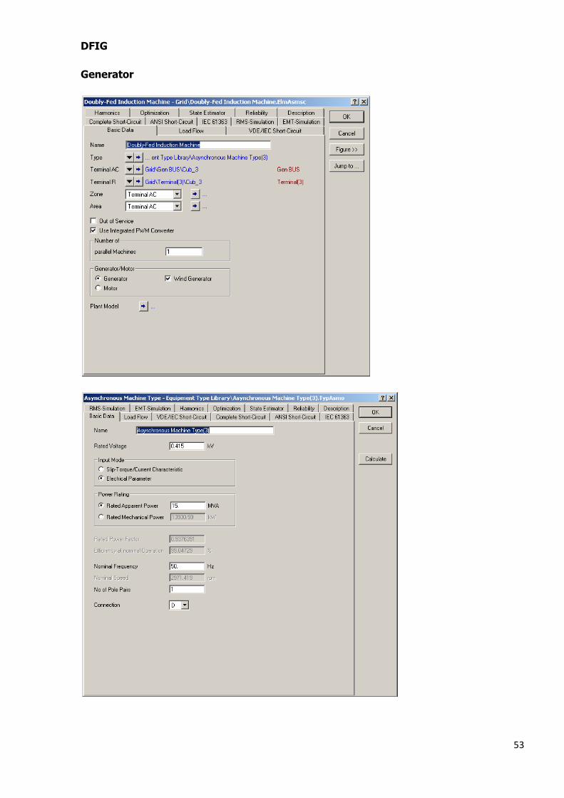
53
DFIG
Generator

54
DFIG
Shunt Filter

55
DFIG
PWM
PWM continue

56
DFIG
Inductor

57
DFIG
3-winding transformer

58
Running Simulation

59

60

61

62
DFIG error message

63
Reference
[1] DIgSILENT GmbH, “DIgSILENT PowerFactory V14.0-User Manual,” DIgSILENT GmbH,
2008 Wind Energy
[2] Renewable Energy Scenarios for Western Australia, WWW.sen.asn.au
[3] Australian Energy Resource Assessment-Chapter-9-Wind Energy
[4] Australia’s renewable energy future, January 2010,Australian Academy of Science 2009
[5] www.ramblingsdc.net/Australia/WindWA.html
[6] http://cleanenergyaustralareport.com.au/technologies/wind-2 ,
[7] http://adl.brs.gov.au/data/warehouse/pe_aera_d9aae_002/aeraCh_08.pdf
[8] www.science.org.au/reports/documents/Ausewnewableenergyfuture.pdf
[9]
http://www.accc.gov.au/content/item.phtml?itemId=916636&nodeId=9ad10c1039e92f6
09847eb3d6201a8c4&fn=Chapter%207%20Beyond%20the%20national%20electricity%20mark
et.pdf
[10] www.energyaction.com.au/nem-swis-comparison.html
[11] Zoran Bozic et al, “Technical rules”, Perth, Wesern Power, 2007
[12] Wind Integration:International Experience, WP2: Review of Grid
Codes,www.aemo.com.au
[13] de Oliveira, J.T.; de Medeiros, M.F.; Oliveira, C.B.M.; , "Development of Modules for
Transient Stability Studies of Power Systems with Wind Turbines in Different Simulation
Platforms," Transmission & Distribution Conference and Exposition: Latin America, 2006.
TDC '06. IEEE/PES , vol., no., pp.1-6, 15-18 Aug. 2006
[14] http://cdn.intechweb.org/pdfs/12519.pdf
[15] Zhao, S.; Qureshi, W.A.; Nair, N.C.; , "Influence of DFIG models on fault current
calculation and protection coordination," Power and Energy Society General Meeting,
2011 IEEE , vol., no., pp.1-8, 24-29 July 2011
[16] wind turbine modelling, www.springer.com/978-1-84800-315-6

64
[17] Review of Contemporary Wind Turbine Concepts and their Market Penetration, Anaca
D.Hansen, Florin lov+, Frede Blaabjerg and Lars H. Hansen
[18] Calais, M.(2011).ENG421 Unit notes. Perth,WA, Australia: Murdoch University
[19] Ackermann, T.(2005). Wind Power in Power System. John Wiley & Sons
[20] http://www.ni.com/white-paper/8189/en [Accessed: 25/10/2012]
[21] http://www.cee.dtu.dk/upload/centre/cet/projekter/03-par-thesis.pdf
[22] Hingorani, N. And Gyugyi, L., “Concepts and technology of flexible AC transmission
systems”, Understanding FACTS, p.210,p.136
[24] Vijay K. Sood “HVDC and FACTS Controllers”, Application of Static Converters in Power
Systems
[23] Xiao-Ping Zhang, Christian Rehtanz, Bikash PalFlexible AC Transmission Systems: Modelling and Contro
[25] K.R.Padiyar, “FACTS controllers in power transmission and distribution”
[26] Improvement of Transmission line power transfer capability,case study-A.Abu Siada and
Chatura Karunar,Electrical and cimputer engineering department,curtin university,WA
western power,perth, Western Australia
[27] Aziz, T.; Hossain, M.J.; Saha, T.K.; Mithulananthan, N.; , "Stability evaluation of
distributed generator integrated system with index based placement of STATCOM,"
Innovative Smart Grid Technologies Asia (ISGT), 2011 IEEE PES , vol., no., pp.1-8, 13-
16 Nov. 2011
[28] http://www.britannica.com/EBchecked/media/125134/Components-of-a-wind-turbine
[29] http://www.icrepq.com/icrepq%2711/635-leao.pdf
[30] http://en.wikipedia.org/wiki/File:GlobalWindPowerCumulativeCapacity.png
[31] Tomas Pertru, “modelling of wind turbine for power system studies
[32] Brendan Fidock, “ The A1 Wind Farm: An investigation into the voltage control, network
support capability and stability of the A1 distribution network,15/5/2010]
[33] Michael Wiktora, “ An investigation in the voltage response and fault handling
capabilities of an Induction Generator Wind Turbine on the A1 Distribution Network,June
2011

65
[34] Gao Xiang; Wang Gang; Wu Zhengrong; Li Haifeng; , "Fault current contributions of
doubly fed induction generator wind turbines under different control strategies,"
Advanced Power System Automation and Protection (APAP), 2011 International
Conference on , vol.2, no., pp.1209-1214, 16-20 Oct. 2011
[35] Zhao, S.; Nair, Nirmal-Kumar C.; , "Behavior of doubly-fed induction generator unit
during system disturbance," Power Engineering Conference, 2008. AUPEC '08.
Australasian Universities , vol., no., pp.1-6, 14-17 Dec. 2008
[36] Kayikci, M.; Milanovic, J.V.; , "Reactive Power Control Strategies for DFIG-Based Plants,"
Energy Conversion, IEEE Transactions on , vol.22, no.2, pp.389-396, June 2007
[37] Francisco Diaz Gonzalez, Marcela Martinez-Rojas, Andreas Sumper, Oriol Gomis-
Bellmunt, Lluis Trilla, “Strategies for Reactive Power Control in Wind Farms with
STATCOM
[38] http://cdn.intechweb.org/pdfs/12519.pdf[Accessed:12/11/2012]
[39] http://www.rpc.com.au/pdf/wind4.pdf[Accessed: 9/10/2012]