inverse scattering and calderón's...

Theorem Lemma

Inverse scattering and Calderon’s problem

Alberto Ruiz,(UAM)

An o. f. c.. Luminy April 2015

April 13, 2015

Alberto Ruiz,(UAM) An o. f. c.. Luminy April 2015 Inverse scattering and Calderon’s problem

Introduction. The Scattering Problem

Scattering is a part of the theory of perturbations. It trays toobtain information for a quantum hamiltonian H which is seen as aperturbation of an other H0 which usually is called the ”freehamiltonian”.We consider here the simplest case of the Schrodinger equation inRn for an electrical potential V (x), given by H = ∆ + V (x) andthe free one H0 = ∆.We will study to basic problems that were the background of thepowerful recent development of the field of Inverse Problems: TheGelfand-Fadeev Scattering problem and the Calderon electricalimpedance tomography problem.


Introduction. The Scattering Problem

The point is to describe the perturbation, given by the potential Vfrom external measurement to the object or by far field profiles ofsome special solutions that can be perturbations of solutions of thefree system.This measurements can be described by two operators :1. The Dirichlet to Neumann operator on the boundary or2. The scattering operator which can be obtained by comparisonof the evolution of the two operators asymptotically in time ( theexistence of such operators is one of the problem in Spectral theoryof operators).In this presentation we will study the stationary point of view andlater on we will comment the evolution approach.


Introduction. The Schrodinger equation

In the case of Schrodinger or potential scattering we assume thatV (x) = q(x) ∈ Lp for some p. The scattering solution of wavenumber k is the solution of the problem

(∆ + k2)u = V (x)u

u = ui + us

us satisfies the outgoing Sommerfeld radiation condition (S.R.C)

(1)The SRC is given by the asymptotic

d

drus − ikus = o(r−

n−12 ), (2)

when |x | = r →∞.ui is an entire solution of the free hamiltonian, the homogeneousHelmholtz equation; this is the case of Herglotz wave functionswhich are superpositions of plane waves

ui (x) = u0(k , θ, x) = e ikθ·x , (3)


The scattering solution u = u(k , θ, x) is a solution of theHelmholtz equation in the exterior of the support of V and so isthe scattered solution us . Since it satisfies the S.R.C., it has thefollowing asymptotics as |x | → ∞:

us(x) = cnk(n−3)/2 e ik|x |

|x |(n−1)/2u∞(k, θ,

x

|x |) + o(|x |−(n−1)/2) (4)

The function u∞(k, θ, ω), is known as the scattering amplitude orfar field pattern, it represents the measurements in the inversescattering problem: The influence of the perturbation in the freesolution ui . It is the response of the perturbation to the planewave with energy k2 and wave front direction θ.The problem in inverse scattering deals with the recovery of theunknown potential V from the set of scattering data u∞(k , θ, ω)for sets of energies k2, incident directions θ ∈ Sn−1 andmeasurements directions ω ∈ Sn−1.


Program of the course

The problem will be approached by the following steps:

1 The direct problem. The unique continuation principle

2 Calderon Problem.

3 Estimates for the free resolvent and consequences.

4 Inverse scattering. Other problems


The direct problem

The way of constructing the scattering solutions is by mean of theso called Lippmann-Schwinger integral equation. We are going tostate this equation, to sketch the proof of existence of the solutionand to get an expression for the far field pattern which will beuseful for our purposes.Let us remark the equation satisfied by us ,

(∆ + k2)us = Vui + Vus (5)

The resolvent of the free problem gives the solution of(∆ + k2)u = f

u outgoing S.R.C(6)


The free resolvent

The solution is given by convolution with the outgoingfundamental solution,

Φk(|x |) =

∫Rn

e ikx ·ξ

−|ξ|2 + k2 + i0dξ.

This kernel has an explicit expression in term of Bessel-Hankelfunctions:

Φ(x) = cnk(n−2)/2

H(1)(n−2)/2(k|x |)|x |(n−2)/2

, where cn =1

2i(2π)(n−2)/2. (7)

In the case of n = 3 this can be written as

Φ(x) =e ik|x |

4π|x |. (8)

We call this the Resolvent operator R+ = R+(k2):


The direct problem

If we apply the resolvent to (5), since us is outgoing, we obtain

us = R+(Vu).

This is the Lippmann-Schwinger integral equation

us(x) =

∫Rn

Φk(x , y)V (y)(ui (y) + us(y))dy (9)

Denote < x >= (1 + |x |2)1/2.

Theorem

Let V ∈ Lr , real, compactly supported with r > n/2, and k > 0.Then there exists a unique solution us of the Lippmann-Schwingerintegral equation such that: us ∈W s,p′(< x >−β dx), wheres < 2− n/r and 1/p − 1/p′ = 1/r , and β is some exponentdepending on r such that β < 1/2 if r <∞.


The direct problem. Existence and estimates

Proof: Take Tk the operator defined as Tk(ψ) = R+(Vψ). Writethe Lippmann-Schwinger equation as

us = Tk(ui + us) = R+(Vui ) + Tk(us)

We use Fredholm theorem.To prove that Tk is compact in W = W s,p′(< x >−β dx) we usethe following estimate, which will be studied in the next session.

Theorem

Let 0 ≤ 1/p − 1/p′ = 1/r ≤ 2/n if n > 2 or 0 ≤ 1/p − 1/p′ < 1for n = 2. Let k > 0 and 0 ≤ s ≤ 2− n/r . Then there exists a βdepending on r and β < 1/2 if r <∞, such that

‖R+(k2)f ‖W s,p′ (<x>−βdx) ≤ C (k)‖f ‖Lp(<x>βdx) (10)


The compactness of Tk follows from this theorem, Holderinequality and Rellich compactness theorem.Now to obtain the existence we need to prove that the onlysolution in W s,p′(< x >−β dx) of the integral equation u = Tk(u)is u = 0. To prove this, notice that u is a solution of the equation(∆ + k2)u = Vu and since V is compactly supported we can useRellich uniqueness theorem

Theorem

Let D = Rn \ Ω be an exterior domain C2, assume that u is aC2(D) ∪ C(D) outgoing solution of (∆ + k2)u = 0 such that

=∫∂Ω

u∂u

∂ν≥ 0, (11)

where ν is the normal to D pointing out of D, then u vanishes in D


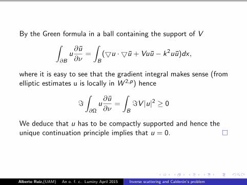
By the Green formula in a ball containing the support of V∫∂B

u∂u

∂ν=

∫B

(5u · 5u + Vuu − k2uu)dx ,

where it is easy to see that the gradient integral makes sense (fromelliptic estimates u is locally in W 2,p) hence

=∫∂Ω

u∂u

∂ν=

∫B=V |u|2 ≥ 0

We deduce that u has to be compactly supported and hence theunique continuation principle implies that u = 0.


The far field pattern

Let start with the scattering interpretation of the Fourier transform.

Proposition

Let v be an outgoing solution of the inhomogeneous Helmholtzequation with a source f ,

∆v + k2v = f ,

where f ∈ L2n/(n+2) is compactly supported. Then v can bewritten when |x | → ∞ as

v(x) = Ck(n−3)/2 e ik|x |

|x |(n−1)/2v∞(k , x/|x |) + o(|x |−(n−1)/2)

and the far field pattern is given by

v∞(k , x/|x |) = f (kx/|x |) (12)


Proof:

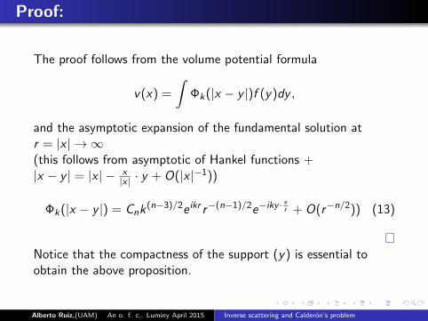
The proof follows from the volume potential formula

v(x) =

∫Φk(|x − y |)f (y)dy ,

and the asymptotic expansion of the fundamental solution atr = |x | → ∞(this follows from asymptotic of Hankel functions +|x − y | = |x | − x

|x | · y + O(|x |−1))

Φk(|x − y |) = Cnk(n−3)/2e ikr r−(n−1)/2e−iky ·

xr + O(r−n/2)) (13)

Notice that the compactness of the support (y) is essential toobtain the above proposition.


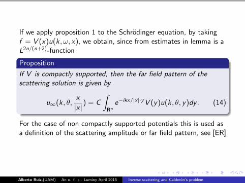
If we apply proposition 1 to the Schrodinger equation, by takingf = V (x)u(k, ω, x), we obtain, since from estimates in lemma is aL2n/(n+2)-function

Proposition

If V is compactly supported, then the far field pattern of thescattering solution is given by

u∞(k , θ,x

|x |) = C

∫Rn

e−ikx/|x |·yV (y)u(k , θ, y)dy . (14)

For the case of non compactly supported potentials this is used asa definition of the scattering amplitude or far field pattern, see [ER]


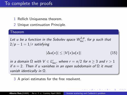
To complete the proofs

1 Rellich Uniqueness theorem.

2 Unique continuation Principle.

Theorem

Let u be a function in the Sobolev space W 2,ploc , for p such that

2/p − 1 = 1/r satisfying

|∆u(x)| ≤ |V (x)u(x)| (15)

in a domain Ω with V ∈ Lrloc , where r = n/2 for n ≥ 3 and r > 1if n = 2. Then if u vanishes in an open subdomain of Ω it mustvanish identically in Ω.

3 A priori estimates for the free resolvent.


The unique continuation principle

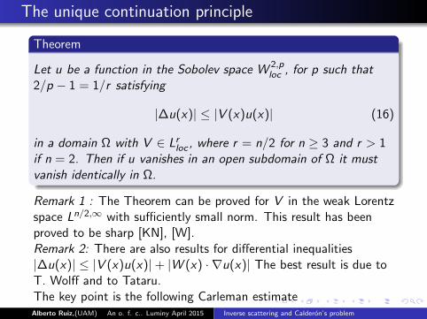
Theorem

Let u be a function in the Sobolev space W 2,ploc , for p such that

2/p − 1 = 1/r satisfying

|∆u(x)| ≤ |V (x)u(x)| (16)

in a domain Ω with V ∈ Lrloc , where r = n/2 for n ≥ 3 and r > 1if n = 2. Then if u vanishes in an open subdomain of Ω it mustvanish identically in Ω.

Remark 1 : The Theorem can be proved for V in the weak Lorentzspace Ln/2,∞ with sufficiently small norm. This result has beenproved to be sharp [KN], [W].Remark 2: There are also results for differential inequalities|∆u(x)| ≤ |V (x)u(x)|+ |W (x) · ∇u(x)| The best result is due toT. Wolff and to Tataru.The key point is the following Carleman estimateAlberto Ruiz,(UAM) An o. f. c.. Luminy April 2015 Inverse scattering and Calderon’s problem

The Carleman estimate

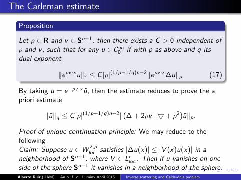
Proposition

Let ρ ∈ R and v ∈ Sn−1, then there exists a C > 0 independent ofρ and v , such that for any u ∈ C∞0 if with p as above and q itsdual exponent

‖eρv ·xu‖q ≤ C |ρ|(1/p−1/q)n−2‖eρv ·x∆u‖p (17)

By taking u = e−ρv ·x u, then the estimate reduces to prove the apriori estimate

‖u‖q ≤ C |ρ|(1/p−1/q)n−2‖(∆ + 2ρv · 5+ ρ2)u‖p.

Proof of unique continuation principle: We may reduce to thefollowingClaim: Suppose u ∈W 2,p

loc satisfies |∆u(x)| ≤ |V (x)u(x)| in aneighborhood of Sn−1, where V ∈ Lrloc . Then if u vanishes on oneside of the sphere Sn−1 it vanishes in a neighborhood of the sphere.Alberto Ruiz,(UAM) An o. f. c.. Luminy April 2015 Inverse scattering and Calderon’s problem

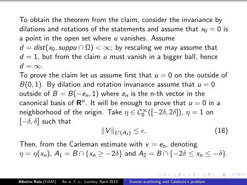
To obtain the theorem from the claim, consider the invariance bydilations and rotations of the statements and assume that x0 = 0 isa point in the open set where u vanishes. Assumed = dist(x0, suppu ∩ Ω) <∞; by rescaling we may assume thatd = 1, but from the claim u must vanish in a bigger ball, henced =∞.To prove the claim let us assume first that u = 0 on the outside ofB(0, 1). By dilation and rotation invariance assume that u = 0outside of B = B(−en, 1) where en is the n-th vector in thecanonical basis of Rn. It will be enough to prove that u = 0 in aneighborhood of the origin. Take η ∈ C∞0 ([−2δ, 2δ]), η = 1 on[−δ, δ] such that

‖V ‖Lr (A1) ≤ ε. (18)

Then, from the Carleman estimate with v = en, denotingη = η(xn), A1 = B ∩xn ≥ −2δ and A2 = B ∩−2δ ≤ xn ≤ −δ.


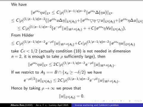
We have

‖eρxnηu‖Lq ≤ C |ρ|(1/p−1/q)n−2‖eρxn∆(ηu)‖Lp

≤ C |ρ|(1/p−1/q)n−2(‖eρxnu∆η‖Lp(A2)+‖eρxn5η·5u‖Lp(A2)+‖eρxnη∆u‖Lp(A1))

≤ C |ρ|(1/p−1/q)n−2(e−ρδ‖u‖W 1,p(A1) + +C‖eρxnηVu‖Lp(A1)),

From Holder

≤ C |ρ|(1/p−1/q)n−2e−ρδ‖u‖W 1,p(A1)+Cε|ρ|(1/p−1/q)n−2‖eρxnηu‖Lq(A1)

take Cε < 1/2 (actually condition (18) is not needed in dimensionn = 2, it is enough to take ρ sufficiently large), then

‖eρxnηu‖Lq ≤ 2C |ρ|(1/p−1/q)n−2e−ρδ‖u‖W 1,p(A1).

If we restrict to A3 == B ∩ xn ≥ −δ/2 we have

e−ρδ/2‖u‖Lq(A3) ≤ 2C |ρ|(1/p−1/q)n−2e−ρδ‖u‖W 1,p(A1).

Hence by taking ρ→∞ we prove that

‖u‖Lq(A3) = 0.


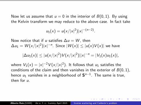
Now let us assume that u = 0 in the interior of B(0, 1). By usingthe Kelvin transform we may reduce to the above case. In fact take

u1(x) = u(x/|x |2)|x |−(n−2).

Now notice that if u satisfies ∆u = W , then∆u1 = W (x/|x |2)|x |−n. Since |W (x)| ≤ |u(x)V (x)| we have

|∆u1(x)| ≤ |u(x/|x |2)V (x/|x |2)||x |−n = |V1(x)u1(x)|,

where V1(x) = |x |−2V (x/|x |2). It follows that u1 satisfies theconditions of the claim and then vanishes in the exterior of B(0, 1),hence u1 vanishes in a neighborhood of Sn−1. The same is true,then for u.


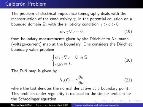
Calderon Problem

The problem of electrical impedance tomography deals with thereconstruction of the conductivity γ, in the potential equation on abounded domain Ω, with the ellipticity condition γ > c > 0,

div γ∇u = 0, (19)

from boundary measurements given by yhe Dirichlet to Neumann(voltage-current) map at the boundary. One considers the Dirichletboundary value problem

div γ∇u = 0 in Ω

u|∂Ω = f .(20)

The D-N map is given by

Λγ(f ) = γ∂u

∂ν(21)

where the last denotes the normal derivative at a boundary point.This problem under regularity is reduced to the similar problem forthe Schrodinger equation.In this presentation we assume that 0 is not a Dirichlet eigenvaluein order to prove the existence of a unique weak solution of theDirichlet boundary value problem.


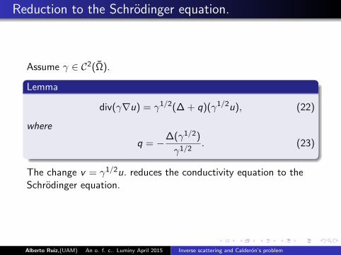
Reduction to the Schrodinger equation.

Assume γ ∈ C2(Ω).

Lemma

div(γ∇u) = γ1/2(∆ + q)(γ1/2u), (22)

where

q = −∆(γ1/2)

γ1/2. (23)

The change v = γ1/2u. reduces the conductivity equation to theSchrodinger equation.


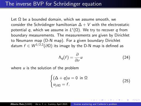
The inverse BVP for Schrodinger equation

Let Ω be a bounded domain, which we assume smooth, weconsider the Schrodinger hamiltonian ∆ + V with the electrostaticpotential q, which we assume in Lr (Ω). We try to recover q fromboundary measurements. The measurements are given by Dirichletto Neumann map (D-N map). For a given boundary Dirichletdatum f ∈W 1/2,2(∂Ω) its image by the D-N map is defined as

Λq(f ) =∂

∂νu (24)

where u is the solution of the problem(∆ + q)u = 0 in Ω

u|∂Ω = f .(25)


Since 0 could be an eigenvalue of the Dirichlet operator, theuniqueness of the above problem can not in general be proved andhence the D-N not need to be a map. In order to avoid thisconstrain, we are going to substitute the D-N map by the so called”Cauchy data set” of q which is defined by

Cq = (u|∂Ω,∂

∂νu) : u ∈W 1,2(Ω), (∆ + q)u = 0 (26)

Remark that in the case that the D-N map exists, Cq is a graph. Ingeneral we may claim

Proposition

Let q ∈ Lr , with r ≥ n/2, then

Cq ⊂W 1/2,2(∂Ω)×W−1/2,2(∂Ω) (27)


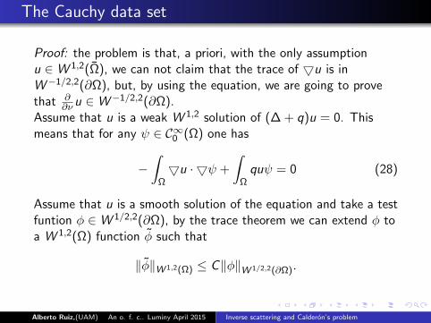
The Cauchy data set

Proof: the problem is that, a priori, with the only assumptionu ∈W 1,2(Ω), we can not claim that the trace of 5u is inW−1/2,2(∂Ω), but, by using the equation, we are going to provethat ∂

∂ν u ∈W−1/2,2(∂Ω).Assume that u is a weak W 1,2 solution of (∆ + q)u = 0. Thismeans that for any ψ ∈ C∞0 (Ω) one has

−∫

Ω5u · 5ψ +

∫Ωquψ = 0 (28)

Assume that u is a smooth solution of the equation and take a testfuntion φ ∈W 1/2,2(∂Ω), by the trace theorem we can extend φ toa W 1,2(Ω) function φ such that

‖φ‖W 1,2(Ω) ≤ C‖φ‖W 1/2,2(∂Ω).


By the Green formula∫∂Ω

∂

∂νuφdσ =

∫Ω

(5u · 5φ) +

∫Ω

∆uφ

=

∫Ω

(5u · 5φ)−∫

Ω(quφ)

(29)

Hence by Holder inequality

|∫∂Ω

∂

∂νuφdσ| ≤ ‖ 5 u‖2‖ 5 φ‖2 + ‖q‖r‖u‖p′‖φ‖p′ ,

where 1/r + 1/p′ + 1/p′ = 1 and 1/p − 1/p′ = 1/r .Since we have 1/r = 1− 2/p′ ≤ 2/n, then 1/2− 1/p′ ≤ 1/n andwe can use the Sobolev embedding, ‖φ‖p′ ≤ C‖φ‖W 1,2(Ω), whichtogether with the trace estimate give us:

|∫∂Ω

∂

∂νuφdσ| ≤ C‖ u‖W 1,2‖φ‖W 1/2,2(∂Ω).

This proves that the normal derivative can be defined, from (29)by density, as an element of W−1/2,2(∂Ω), with the onlyassumption u ∈W 1,2(Ω).Alberto Ruiz,(UAM) An o. f. c.. Luminy April 2015 Inverse scattering and Calderon’s problem

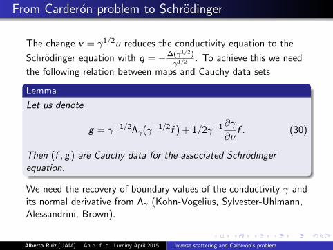
From Carderon problem to Schrodinger

The change v = γ1/2u reduces the conductivity equation to the

Schrodinger equation with q = −∆(γ1/2)

γ1/2 . To achieve this we need

the following relation between maps and Cauchy data sets

Lemma

Let us denote

g = γ−1/2Λγ(γ−1/2f ) + 1/2γ−1∂γ

∂νf . (30)

Then (f , g) are Cauchy data for the associated Schrodingerequation.

We need the recovery of boundary values of the conductivity γ andits normal derivative from Λγ (Kohn-Vogelius, Sylvester-Uhlmann,Alessandrini, Brown).


Uniqueness of the inverse problem

Now we can state the main result of this section, the uniquenes ofthe inverse boundary value problem. This is a Lr -version ofSylvester and Uhlmann’s pioneering result due to Jerison andKenig and Chanillo.

Theorem

Let q1 and q2 be functions in Lr (Ω), r > n/2, n ≥ 3. AssumeCq1 = Cq2 then q1 = q2.

The proof is based on the existence of Calderon approximatedsolutions :


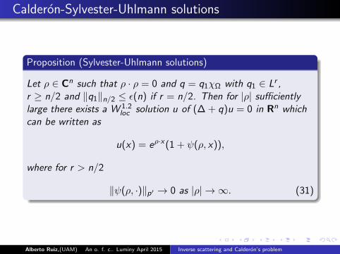
Calderon-Sylvester-Uhlmann solutions

Proposition (Sylvester-Uhlmann solutions)

Let ρ ∈ Cn such that ρ · ρ = 0 and q = q1χΩ with q1 ∈ Lr ,r ≥ n/2 and ‖q1‖n/2 ≤ ε(n) if r = n/2. Then for |ρ| sufficientlylarge there exists a W 1.2

loc solution u of (∆ + q)u = 0 in Rn whichcan be written as

u(x) = eρ·x(1 + ψ(ρ, x)),

where for r > n/2

‖ψ(ρ, ·)‖p′ → 0 as |ρ| → ∞. (31)


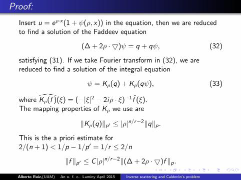
Proof:

Insert u = eρ·x(1 + ψ(ρ, x)) in the equation, then we are reducedto find a solution of the Faddeev equation

(∆ + 2ρ · 5)ψ = q + qψ, (32)

satisfying (31). If we take Fourier transform in (32), we arereduced to find a solution of the integral equation

ψ = Kρ(q) + Kρ(qψ), (33)

where Kρ(f )(ξ) = (−|ξ|2 − 2iρ · ξ)−1f (ξ).The mapping properties of Kρ we use are

‖Kρ(q)‖p′ ≤ |ρ|n/r−2‖q‖p.

This is the a priori estimate for2/(n + 1) < 1/p − 1/p′ = 1/r ≤ 2/n

‖f ‖p′ ≤ C |ρ|n/r−2‖(∆ + 2ρ · 5)f ‖p.


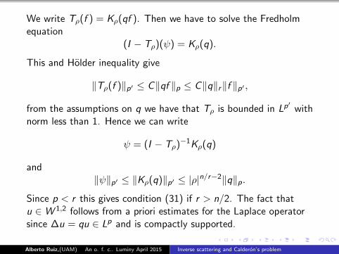
We write Tρ(f ) = Kρ(qf ). Then we have to solve the Fredholmequation

(I − Tρ)(ψ) = Kρ(q).

This and Holder inequality give

‖Tρ(f )‖p′ ≤ C‖qf ‖p ≤ C‖q‖r‖f ‖p′ ,

from the assumptions on q we have that Tρ is bounded in Lp′

withnorm less than 1. Hence we can write

ψ = (I − Tρ)−1Kρ(q)

and‖ψ‖p′ ≤ ‖Kρ(q)‖p′ ≤ |ρ|n/r−2‖q‖p.

Since p < r this gives condition (31) if r > n/2. The fact thatu ∈W 1,2 follows from a priori estimates for the Laplace operatorsince ∆u = qu ∈ Lp and is compactly supported.


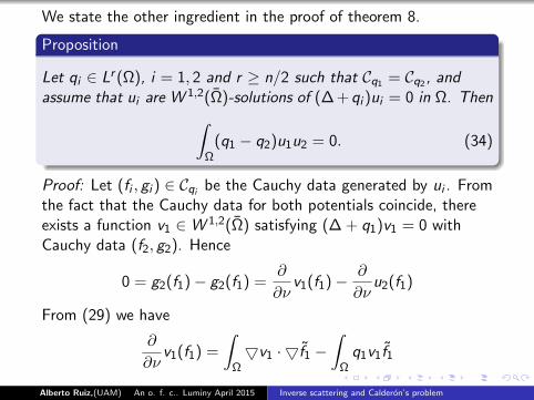
We state the other ingredient in the proof of theorem 8.

Proposition

Let qi ∈ Lr (Ω), i = 1, 2 and r ≥ n/2 such that Cq1 = Cq2 , andassume that ui are W 1,2(Ω)-solutions of (∆ +qi )ui = 0 in Ω. Then∫

Ω(q1 − q2)u1u2 = 0. (34)

Proof: Let (fi , gi ) ∈ Cqi be the Cauchy data generated by ui . Fromthe fact that the Cauchy data for both potentials coincide, thereexists a function v1 ∈W 1,2(Ω) satisfying (∆ + q1)v1 = 0 withCauchy data (f2, g2). Hence

0 = g2(f1)− g2(f1) =∂

∂νv1(f1)− ∂

∂νu2(f1)

From (29) we have

∂

∂νv1(f1) =

∫Ω5v1 · 5f1 −

∫Ωq1v1f1


We may choose the extension f1 = u1, hence

∂

∂νv1(f1) =

∫Ω5v1 · 5u1 −

∫Ωq1v1u1

=∂

∂νu1(f2)

since v1 is an extension of f2. Then we have

0 =∂

∂νu1(f2)− ∂

∂νu2(f1)

=

∫Ω5u1 · 5u2 −

∫Ωq1u1u2 −

∫Ω5u2 · 5u1 +

∫Ωq2u2u1

This proves the proposition.


Proof of uniqueness theorem :

Fix ξ ∈ Rn and take the two complex vectors ρ1 = l + i(ξ + m)and ρ2 = −l + i(ξ −m), where l , m and ξ are vectors in Rn

orthogonal to each other and |l | = |ξ + m|. From proposition 5 wecan take for i = 1, 2 a solution of (∆ + qi )ui = 0 of the formui = eρi ·x(1 + ψi (ρ, x)). Then from proposition 25 we have

0 =

∫Ω

(q1−q2)u1u2 =

∫Ω

(q1−q2)eρ1·x(1+ψ1(ρ, x))eρ2·x(1+ψ2(ρ, x))dx

=

∫Ω

(q1 − q2)e2iξ·xdx +

∫Ω

(q1 − q2)e2iξ·xψ1(ρ1, x)(1 + ψ2(ρ2, x))

+

∫Ω

(q1 − q2)e2iξ·xψ2(ρ2, x)(1 + ψ1(ρ1, x)).

But

|∫

Ωqie

2iξ·xψ2(ρ2, x)(1 + ψ1(ρ1, x))| ≤ ‖qi‖r‖ψ2‖p′‖1 + ψ2‖Lp′ (Ω)

tends to zero as |ρ| = c |l | tends to ∞, hence we obtainq1 − q2 = 0.Alberto Ruiz,(UAM) An o. f. c.. Luminy April 2015 Inverse scattering and Calderon’s problem

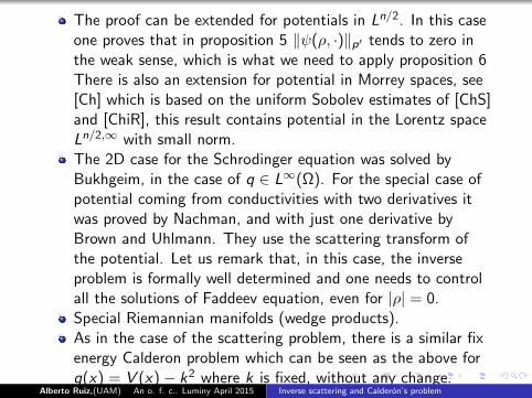
The proof can be extended for potentials in Ln/2. In this caseone proves that in proposition 5 ‖ψ(ρ, ·)‖p′ tends to zero inthe weak sense, which is what we need to apply proposition 6There is also an extension for potential in Morrey spaces, see[Ch] which is based on the uniform Sobolev estimates of [ChS]and [ChiR], this result contains potential in the Lorentz spaceLn/2,∞ with small norm.The 2D case for the Schrodinger equation was solved byBukhgeim, in the case of q ∈ L∞(Ω). For the special case ofpotential coming from conductivities with two derivatives itwas proved by Nachman, and with just one derivative byBrown and Uhlmann. They use the scattering transform ofthe potential. Let us remark that, in this case, the inverseproblem is formally well determined and one needs to controlall the solutions of Faddeev equation, even for |ρ| = 0.Special Riemannian manifolds (wedge products).As in the case of the scattering problem, there is a similar fixenergy Calderon problem which can be seen as the above forq(x) = V (x)− k2 where k is fixed, without any change.


Back to Calderon problem

Regularity: It requires (n ≥ 3) to reduce to Schrodingerequation: Sylverter-Uhlmann, Brown (γ ∈W 3/2)Haberman-Tataru (C1, small Lipschitz norm) Haberman(W 1,n, n = 3, 4), Caro-Roger (Lipschitz n > 4). Newestimates.

2d: Calderon conjecture was solved by Astala and Paivarinta,by using Beltrami equation.

Other Schrodinger equations. Magnetic potentials. Otherintegral transform.

Partial data problems and local data problem.


Summary

Estimates needed:

Resolvent R+(k2)(f ) = (∆ + k2 + i0)−1(f ),

‖R+(k2)f ‖W s,p′ (<x>−βdx) ≤ C (k)‖f ‖Lp(<x>βdx).

Carleman (ρ ∈ R)

‖f ‖q ≤ C |ρ|(1/p−1/q)n−2‖(∆ + 2ρv · 5+ ρ2)f ‖p.

Fadeev (ρ ∈ Cn)

‖f ‖p′ ≤ C |ρ|n/r−2‖(∆ + 2ρ · 5)f ‖p.


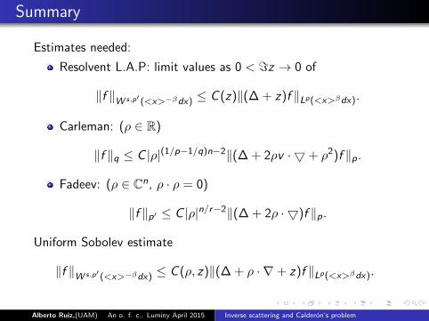
Summary

Estimates needed:

Resolvent L.A.P: limit values as 0 < =z → 0 of

‖f ‖W s,p′ (<x>−βdx) ≤ C (z)‖(∆ + z)f ‖Lp(<x>βdx).

Carleman: (ρ ∈ R)

‖f ‖q ≤ C |ρ|(1/p−1/q)n−2‖(∆ + 2ρv · 5+ ρ2)f ‖p.

Fadeev: (ρ ∈ Cn, ρ · ρ = 0)

‖f ‖p′ ≤ C |ρ|n/r−2‖(∆ + 2ρ · 5)f ‖p.

Uniform Sobolev estimate

‖f ‖W s,p′ (<x>−βdx) ≤ C (ρ, z)‖(∆ + ρ · ∇+ z)f ‖Lp(<x>βdx).


inverse scattering and calderón's...

Documents