)+(1)+(1

)+K(1=G(s)

21

3

ss

s

Inverse Response

Dynamic Response Characteristics of More Complicated Systems

03 If ….fast response

00)=(t slope

3 : zero of transfer functionUse nonlinear regression for fitting data(graphical method not available)

Ch

apte

r 6

response e....invers 03 (see Fig. 6.3)

Ch

apte

r 6

Ch

apte

r 6

For inverse response 1 2 2 1

1 2

0 (6 21)K K

K K

Ch

apte

r 6

2 21

( )( 1)( 2 1)

KG s

s s s s

4 poles (denominator is 4th order polynomial)

More General Transfer Function ModelsC

hap

ter

6

• Poles and Zeros:

• The dynamic behavior of a transfer function model can be characterized by the numerical value of its poles and zeros.

• General Representation of a TF:

There are two equivalent representations:

0

0

(4-40)

mi

iin

ii

i

b s

G s

a s

Ch

apte

r 6 where {zi} are the “zeros” and {pi} are the “poles”.

1 2

1 2

(6-7)m m

n n

b s z s z s zG s

a s p s p s p

• We will assume that there are no “pole-zero” cancellations. That is, that no pole has the same numerical value as a zero.

• Review: in order to have a physically realizable system.n m

Ch

apte

r 6

Time DelaysTime delays occur due to:

1. Fluid flow in a pipe

2. Transport of solid material (e.g., conveyor belt)

3. Chemical analysis

- Sampling line delay

- Time required to do the analysis (e.g., on-line gas chromatograph)

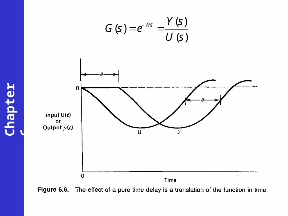
Mathematical description:

A time delay, , between an input u and an output y results in the following expression:

θ

0 for θ

(6-27)θ for θ

ty t

u t t

Ch

apte

r 6

( )( )

( )s Y s

G s eU s

Ch

apte

r 6

H1/Qi has numerator dynamics (see 6-72)

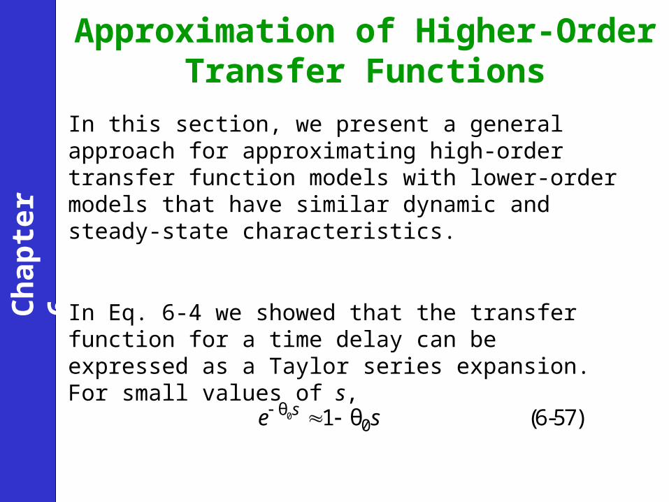
Approximation of Higher-Order Transfer Functions

0θ01 θ (6-57)se s

In this section, we present a general approach for approximating high-order transfer function models with lower-order models that have similar dynamic and steady-state characteristics.

In Eq. 6-4 we showed that the transfer function for a time delay can be expressed as a Taylor series expansion. For small values of s,

Ch

apte

r 6

• An alternative first-order approximation consists of the transfer function,

0

0

θθ

0

1 1(6-58)

1 θs

se

se

where the time constant has a value of

• These expressions can be used to approximate the pole or zero term in a transfer function.

0θ .

Ch

apte

r 6

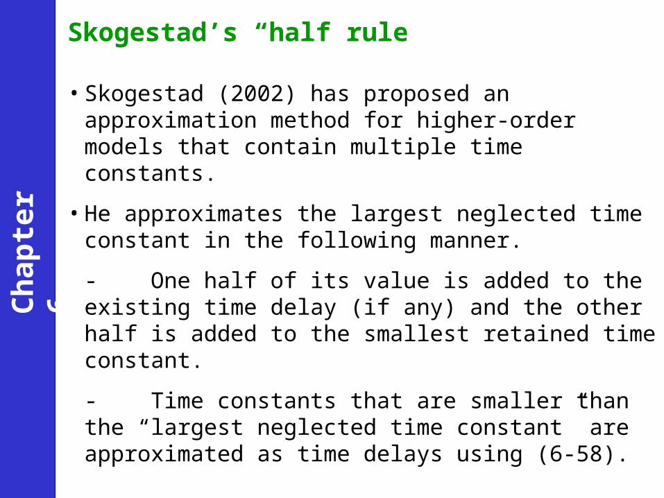
Skogestad’s “half rule”

• Skogestad (2002) has proposed an approximation method for higher-order models that contain multiple time constants.

• He approximates the largest neglected time constant in the following manner.

- One half of its value is added to the existing time delay (if any) and the other half is added to the smallest retained time constant.

- Time constants that are smaller than the “largest neglected time constant” are approximated as time delays using (6-58).

Ch

apte

r 6

Example 6.4

Consider a transfer function:

0.1 1(6-59)

5 1 3 1 0.5 1

K sG s

s s s

Derive an approximate first-order-plus-time-delay model,

θ

(6-60)τ 1

sKeG s

s

using two methods:

(a) The Taylor series expansions of Eqs. 6-57 and 6-58.

(b) Skogestad’s half rule

Ch

apte

r 6

Compare the normalized responses of G(s) and the approximate models for a unit step input.

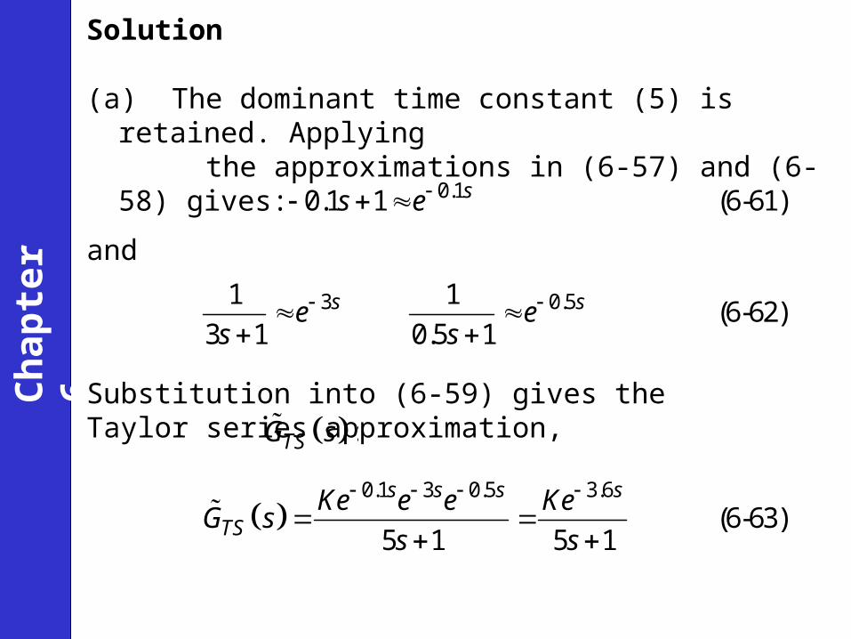
Solution

(a) The dominant time constant (5) is retained. Applying the approximations in (6-57) and (6-58) gives:

0.10.1 1 (6-61)ss e

and

3 0.51 1(6-62)

3 1 0.5 1s se e

s s

Substitution into (6-59) gives the Taylor series approximation, :TSG s

0.1 3 0.5 3.6

(6-63)5 1 5 1

s s s s

TSKe e e Ke

G ss s

Ch

apte

r 6

(b) To use Skogestad’s method, we note that the largest neglected time constant in (6-59) has a value of three.

θ 1.5 0.1 0.5 2.1

Ch

apte

r 6

• According to his “half rule”, half of this value is added to the next largest time constant to generate a new time constant

• The other half provides a new time delay of 0.5(3) = 1.5. • The approximation of the RHP zero in (6-61) provides an

additional time delay of 0.1. • Approximating the smallest time constant of 0.5 in (6-59) by

(6-58) produces an additional time delay of 0.5. • Thus the total time delay in (6-60) is,

τ 5 0.5(3) 6.5.

and G(s) can be approximated as:

2.1

(6-64)6.5 1

s

SkKe

G ss

The normalized step responses for G(s) and the two approximate models are shown in Fig. 6.10. Skogestad’s method provides better agreement with the actual response.

Ch

apte

r 6

Figure 6.10 Comparison of the actual and approximate models for Example 6.4.

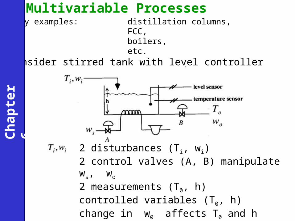
Multivariable Processesmany examples: distillation columns,

FCC,boilers,etc.

Consider stirred tank with level controller

2 disturbances (Ti, wi)2 control valves (A, B) manipulate ws, wo

2 measurements (T0, h)controlled variables (T0, h)change in w0 affects T0 and hchange in ws only affects T0

Ch

apte

r 6

)s(W

)s(W

GG

GG

)s(H

)s(T

0

s

2221

12110

)s(W

)s(HG

)s(W

)s(HG

)s(W

)s(TG

)s(W

)s(TG

022

s21

0

012

s

011

1

)1)(1(

1

2

2222

21

1212

1

1111

s

KG

ss

KG

s

KG

Three non-zero transfer functions

Transfer Function Matrix

From material and energy balances,

Ch

apte

r 6

Ch

apte

r 6

Ch

apte

r 6

Normal method, but interactions may presenttuning problems.

In multivariable control, interactions are treated,but controller design is more complicated.

Ch

apte

r 6

Previous chapter Next chapter

Ch

apte

r 6