inverse laplace transform of rational functions using ...zelenko/odelaplacepf.pdf · inverse...
TRANSCRIPT

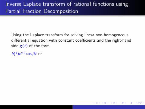
Inverse Laplace transform of rational functions usingPartial Fraction Decomposition
Using the Laplace transform for solving linear non-homogeneousdifferential equation with constant coefficients and the right-handside g(t) of the form
h(t)eαt cosβt or h(t)eαt sinβt,
where h(t) is a polynomial, one needs on certain step to find the
inverse Laplace transform of rational functionsP(s)
Q(s),
where P(s) and Q(s) are polynomials with degP(s) < degQ(s).
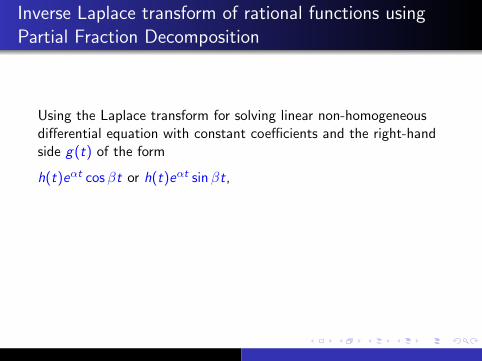
Inverse Laplace transform of rational functions usingPartial Fraction Decomposition
Using the Laplace transform for solving linear non-homogeneousdifferential equation with constant coefficients and the right-handside g(t) of the form
h(t)eαt cosβt or
h(t)eαt sinβt,
where h(t) is a polynomial, one needs on certain step to find the
inverse Laplace transform of rational functionsP(s)
Q(s),
where P(s) and Q(s) are polynomials with degP(s) < degQ(s).
Inverse Laplace transform of rational functions usingPartial Fraction Decomposition
Using the Laplace transform for solving linear non-homogeneousdifferential equation with constant coefficients and the right-handside g(t) of the form
h(t)eαt cosβt or h(t)eαt sinβt,
where h(t) is a polynomial, one needs on certain step to find the
inverse Laplace transform of rational functionsP(s)
Q(s),
where P(s) and Q(s) are polynomials with degP(s) < degQ(s).

Inverse Laplace transform of rational functions usingPartial Fraction Decomposition
The latter can be done by means of the partial fractiondecomposition that you studied in Calculus 2:
One factors the denominator Q(s) as much as possible, i.e. intolinear (may be repeated) and quadratic (may be repeated) factors:
each linear factor corresponds to a real root of Q(s) andeach quadratic factor corresponds to a pair of complex conjugateroots of Q(s).

Inverse Laplace transform of rational functions usingPartial Fraction Decomposition
The latter can be done by means of the partial fractiondecomposition that you studied in Calculus 2:
One factors the denominator Q(s) as much as possible, i.e. intolinear (may be repeated) and quadratic (may be repeated) factors:
each linear factor corresponds to a real root of Q(s) and
each quadratic factor corresponds to a pair of complex conjugateroots of Q(s).

Inverse Laplace transform of rational functions usingPartial Fraction Decomposition
The latter can be done by means of the partial fractiondecomposition that you studied in Calculus 2:
One factors the denominator Q(s) as much as possible, i.e. intolinear (may be repeated) and quadratic (may be repeated) factors:
each linear factor corresponds to a real root of Q(s) andeach quadratic factor corresponds to a pair of complex conjugateroots of Q(s).

Inverse Laplace transform of rational functions usingPartial Fraction Decomposition
The latter can be done by means of the partial fractiondecomposition that you studied in Calculus 2:
One factors the denominator Q(s) as much as possible, i.e. intolinear (may be repeated) and quadratic (may be repeated) factors:
each linear factor corresponds to a real root of Q(s) andeach quadratic factor corresponds to a pair of complex conjugateroots of Q(s).

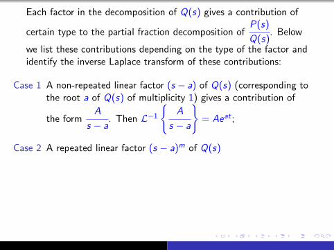
Each factor in the decomposition of Q(s) gives a contribution of
certain type to the partial fraction decomposition ofP(s)
Q(s). Below
we list these contributions depending on the type of the factor andidentify the inverse Laplace transform of these contributions:
Case 1 A non-repeated linear factor (s − a) of Q(s) (corresponding tothe root a of Q(s) of multiplicity 1) gives a contribution of
the formA
s − a. Then L−1
{A
s − a
}= Aeat ;
Case 2 A repeated linear factor (s − a)m of Q(s) (corresponding tothe root a of Q(s) of multiplicity m) gives a contribution
which is a sum of terms of the formAi
(s − a)i, 1 ≤ i ≤ m.
Then L−1
{Ai
(s − a)i
}=
Ai
(i − 1)!t i−1eat ;

Each factor in the decomposition of Q(s) gives a contribution of
certain type to the partial fraction decomposition ofP(s)
Q(s). Below
we list these contributions depending on the type of the factor andidentify the inverse Laplace transform of these contributions:
Case 1 A non-repeated linear factor (s − a) of Q(s)
(corresponding tothe root a of Q(s) of multiplicity 1) gives a contribution of
the formA
s − a. Then L−1
{A
s − a
}= Aeat ;
Case 2 A repeated linear factor (s − a)m of Q(s) (corresponding tothe root a of Q(s) of multiplicity m) gives a contribution
which is a sum of terms of the formAi
(s − a)i, 1 ≤ i ≤ m.
Then L−1
{Ai
(s − a)i
}=
Ai
(i − 1)!t i−1eat ;

Each factor in the decomposition of Q(s) gives a contribution of
certain type to the partial fraction decomposition ofP(s)
Q(s). Below
we list these contributions depending on the type of the factor andidentify the inverse Laplace transform of these contributions:
Case 1 A non-repeated linear factor (s − a) of Q(s) (corresponding tothe root a of Q(s) of multiplicity 1)
gives a contribution of
the formA
s − a. Then L−1
{A
s − a
}= Aeat ;
Case 2 A repeated linear factor (s − a)m of Q(s) (corresponding tothe root a of Q(s) of multiplicity m) gives a contribution
which is a sum of terms of the formAi
(s − a)i, 1 ≤ i ≤ m.
Then L−1
{Ai
(s − a)i
}=
Ai
(i − 1)!t i−1eat ;

Each factor in the decomposition of Q(s) gives a contribution of
certain type to the partial fraction decomposition ofP(s)
Q(s). Below
we list these contributions depending on the type of the factor andidentify the inverse Laplace transform of these contributions:
Case 1 A non-repeated linear factor (s − a) of Q(s) (corresponding tothe root a of Q(s) of multiplicity 1) gives a contribution of
the formA
s − a.
Then L−1
{A
s − a
}= Aeat ;
Case 2 A repeated linear factor (s − a)m of Q(s) (corresponding tothe root a of Q(s) of multiplicity m) gives a contribution
which is a sum of terms of the formAi
(s − a)i, 1 ≤ i ≤ m.
Then L−1
{Ai
(s − a)i
}=
Ai
(i − 1)!t i−1eat ;

Each factor in the decomposition of Q(s) gives a contribution of
certain type to the partial fraction decomposition ofP(s)
Q(s). Below
we list these contributions depending on the type of the factor andidentify the inverse Laplace transform of these contributions:
Case 1 A non-repeated linear factor (s − a) of Q(s) (corresponding tothe root a of Q(s) of multiplicity 1) gives a contribution of
the formA
s − a. Then L−1
{A
s − a
}= Aeat ;
Case 2 A repeated linear factor (s − a)m of Q(s) (corresponding tothe root a of Q(s) of multiplicity m) gives a contribution
which is a sum of terms of the formAi
(s − a)i, 1 ≤ i ≤ m.
Then L−1
{Ai
(s − a)i
}=
Ai
(i − 1)!t i−1eat ;
Each factor in the decomposition of Q(s) gives a contribution of
certain type to the partial fraction decomposition ofP(s)
Q(s). Below
we list these contributions depending on the type of the factor andidentify the inverse Laplace transform of these contributions:
Case 1 A non-repeated linear factor (s − a) of Q(s) (corresponding tothe root a of Q(s) of multiplicity 1) gives a contribution of
the formA
s − a. Then L−1
{A
s − a
}= Aeat ;
Case 2 A repeated linear factor (s − a)m of Q(s)
(corresponding tothe root a of Q(s) of multiplicity m) gives a contribution
which is a sum of terms of the formAi
(s − a)i, 1 ≤ i ≤ m.
Then L−1
{Ai
(s − a)i
}=
Ai
(i − 1)!t i−1eat ;

Each factor in the decomposition of Q(s) gives a contribution of
certain type to the partial fraction decomposition ofP(s)
Q(s). Below
we list these contributions depending on the type of the factor andidentify the inverse Laplace transform of these contributions:
Case 1 A non-repeated linear factor (s − a) of Q(s) (corresponding tothe root a of Q(s) of multiplicity 1) gives a contribution of
the formA
s − a. Then L−1
{A
s − a
}= Aeat ;
Case 2 A repeated linear factor (s − a)m of Q(s) (corresponding tothe root a of Q(s) of multiplicity m)
gives a contribution
which is a sum of terms of the formAi
(s − a)i, 1 ≤ i ≤ m.
Then L−1
{Ai
(s − a)i
}=
Ai
(i − 1)!t i−1eat ;

Each factor in the decomposition of Q(s) gives a contribution of
certain type to the partial fraction decomposition ofP(s)
Q(s). Below
we list these contributions depending on the type of the factor andidentify the inverse Laplace transform of these contributions:
Case 1 A non-repeated linear factor (s − a) of Q(s) (corresponding tothe root a of Q(s) of multiplicity 1) gives a contribution of
the formA
s − a. Then L−1
{A
s − a
}= Aeat ;
Case 2 A repeated linear factor (s − a)m of Q(s) (corresponding tothe root a of Q(s) of multiplicity m) gives a contribution
which is a sum of terms of the form
Ai
(s − a)i, 1 ≤ i ≤ m.
Then L−1
{Ai
(s − a)i
}=
Ai
(i − 1)!t i−1eat ;

Each factor in the decomposition of Q(s) gives a contribution of
certain type to the partial fraction decomposition ofP(s)
Q(s). Below
we list these contributions depending on the type of the factor andidentify the inverse Laplace transform of these contributions:
Case 1 A non-repeated linear factor (s − a) of Q(s) (corresponding tothe root a of Q(s) of multiplicity 1) gives a contribution of
the formA
s − a. Then L−1
{A
s − a
}= Aeat ;
Case 2 A repeated linear factor (s − a)m of Q(s) (corresponding tothe root a of Q(s) of multiplicity m) gives a contribution
which is a sum of terms of the formAi
(s − a)i, 1 ≤ i ≤ m.
Then L−1
{Ai
(s − a)i
}=
Ai
(i − 1)!t i−1eat ;

Each factor in the decomposition of Q(s) gives a contribution of
certain type to the partial fraction decomposition ofP(s)
Q(s). Below
we list these contributions depending on the type of the factor andidentify the inverse Laplace transform of these contributions:
Case 1 A non-repeated linear factor (s − a) of Q(s) (corresponding tothe root a of Q(s) of multiplicity 1) gives a contribution of
the formA
s − a. Then L−1
{A
s − a
}= Aeat ;
Case 2 A repeated linear factor (s − a)m of Q(s) (corresponding tothe root a of Q(s) of multiplicity m) gives a contribution
which is a sum of terms of the formAi
(s − a)i, 1 ≤ i ≤ m.
Then L−1
{Ai
(s − a)i
}=
Ai
(i − 1)!t i−1eat ;

Case 3 A non-repeated quadratic factor (s − α)2 + β2 of Q(s)
(corresponding to the pair of complex conjugate roots α± iβof multiplicity 1) gives a contribution of the form
Cs + D
(s − α)2 + β2.
It is more convenient here to represent it in the following way:Cs + D
(s − α)2 + β2=
A(s − α) + Bβ
(s − α)2 + β2. Then
L−1
{A(s − α) + Bβ
(s − α)2 + β2
}= Aeαt cosβt + Beαt sinβt;

Case 3 A non-repeated quadratic factor (s − α)2 + β2 of Q(s)(corresponding to the pair of complex conjugate roots α± iβof multiplicity 1)
gives a contribution of the formCs + D
(s − α)2 + β2.
It is more convenient here to represent it in the following way:Cs + D
(s − α)2 + β2=
A(s − α) + Bβ
(s − α)2 + β2. Then
L−1
{A(s − α) + Bβ
(s − α)2 + β2
}= Aeαt cosβt + Beαt sinβt;

Case 3 A non-repeated quadratic factor (s − α)2 + β2 of Q(s)(corresponding to the pair of complex conjugate roots α± iβof multiplicity 1) gives a contribution of the form
Cs + D
(s − α)2 + β2.
It is more convenient here to represent it in the following way:
Cs + D
(s − α)2 + β2=
A(s − α) + Bβ
(s − α)2 + β2. Then
L−1
{A(s − α) + Bβ
(s − α)2 + β2
}= Aeαt cosβt + Beαt sinβt;

Case 3 A non-repeated quadratic factor (s − α)2 + β2 of Q(s)(corresponding to the pair of complex conjugate roots α± iβof multiplicity 1) gives a contribution of the form
Cs + D
(s − α)2 + β2.
It is more convenient here to represent it in the following way:Cs + D
(s − α)2 + β2=
A(s − α) + Bβ
(s − α)2 + β2.
Then
L−1
{A(s − α) + Bβ
(s − α)2 + β2
}= Aeαt cosβt + Beαt sinβt;

Case 3 A non-repeated quadratic factor (s − α)2 + β2 of Q(s)(corresponding to the pair of complex conjugate roots α± iβof multiplicity 1) gives a contribution of the form
Cs + D
(s − α)2 + β2.
It is more convenient here to represent it in the following way:Cs + D
(s − α)2 + β2=
A(s − α) + Bβ
(s − α)2 + β2. Then
L−1
{A(s − α) + Bβ
(s − α)2 + β2
}= Aeαt cosβt + Beαt sinβt;

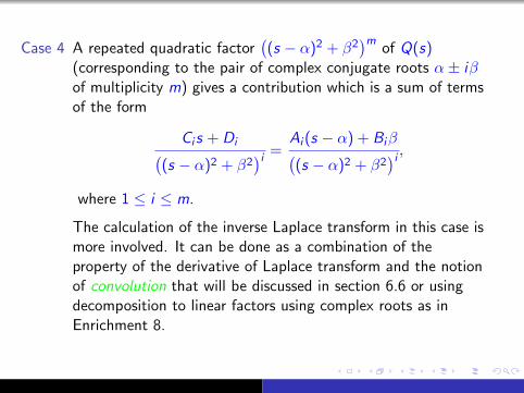
Case 4 A repeated quadratic factor((s − α)2 + β2
)mof Q(s)
(corresponding to the pair of complex conjugate roots α± iβof multiplicity m) gives a contribution which is a sum of termsof the form
Ci s + Di((s − α)2 + β2
)i =Ai (s − α) + Biβ((s − α)2 + β2
)i ,where 1 ≤ i ≤ m.
The calculation of the inverse Laplace transform in this case ismore involved. It can be done as a combination of theproperty of the derivative of Laplace transform and the notionof convolution that will be discussed in section 6.6 or usingdecomposition to linear factors using complex roots as inEnrichment 8.