Inverse Kinematics

• Find the required joint angles to place the robot at a given location

• Places the frame {T} at a point relative to the frame {S}

• Often Can be split into two parts– First find the {W}using transformations relative to {B}

– Then find the inverses to find the joint angles

• In other words GivenFind

• The problem of solving these equation in non-linear– Puma can reach a position with up to 8 different joint solution.

– In general a 6DOF manipulator made of rotary actuator could have 16 solutions.

– The more zero link lengths and the more equal to 0 +-90 the simpler the solution

nθθθθ

T

,,,, 321

0N

Kinematics Preliminaries

• Relation Ship between adjacent links can be described by a transformation matrix as Shown.

• A six DOF manipulator could be described by 7 matrices

• Vectors In R Describe Orientation

• P describes Position

• 16 Values– 4 Trivial

– 3 for position

– 9 for orientation only 3 unique

TTTTT NNN12

312

01

0

1000

100

011

011

2

2

2

orgZ

orgY

orgX

P

PCS

PSC

T R

Loop Closure Equation

• In general all unknowns are on Right – Knowns on Left

– Unknowns multiply each other and are complex.

• can be rewriten in many way– Piepers

– etc

• Some forms will be simpler.– Find Inverse of Wrist

– Wrist Point Robot

TTTTT NTT12

312

01

0

TTTTTTT NT

TTT

TW

123

12

01

0

1 TT WT

TW

Several Methods can be used

• Suppressed Tangent Method

• Suppressed Joint Variables

• Long Form

Number of Solutions

• a1=a2=a5=0 <4

• a3=a5=0 <8

• a3=0 <16

• no ai=0 <16

• If any 3 neighboring joints intersect then there will be a solution.Spherical JointXYZEtc.

Definition

• Linear: For each x there is uniquely one y.Additive and Multiplicative, F(2x)=F(x)+F(x).

• Solvable: Has a unique solution

• Closed Form: Can be computed Algebraically and provides all solutions

• Numerical: Iterative Process

• Algebraic: Uses Algebraic Identities to substitute and to solve

• Geometric: Utilizes Geometric Relationships Law of Sines, etc

• Sub-Space: Smaller RegionCircle in a planeSphere in XYZ space

Main Methods

• Numerical– Iterative

• Closed Form– Algebraic

– Geometric

• All 6DOF manipulators in a single serial chain are solvable numerically

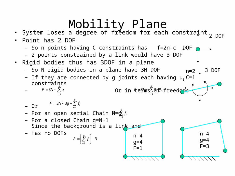
Mobility Plane• System loses a degree of freedom for each constraint • Point has 2 DOF

– So n points having C constraints has f=2n-c DOF– 2 points constrained by a link would have 3 DOF

• Rigid bodies thus has 3DOF in a plane– So N rigid bodies in a plane have 3N DOF– If they are connected by g joints each having ui constraints– Or in terms of freedoms

– Or– For an open serial Chain N=g– For a closed Chain g=N+1

Since the background is a link and– Has no DOFs

2 DOF

n=4g=4F=1

3 DOFn=2C=1

g

iiuNF

1

3

g

iifNF

1

33

g

iifgNF

1

33

g

iifF

1

n=4g=4F=3

31

g

iifF

Mobility Space

• Point had 3DOF

• Rigid Body is 3 Points Connected by Constraints– F=3n-C F=9-3=6

– Rigid Body has 6 DOF

• So for a system of bodies

• Counting Ground as a Body and writing in terms of freedoms

• For Open Loop chain

• Or for Closed Loop have one more joint than links

g

iifgNF

1

' 16

g

iiuNF

1

6

61

g

iifF

g

iifF

1

Inverse Kinematics Heuristic

1. Equate the General position transformation matrix to the manipulator transformation matrix. In some cases this can be a simplified matrix

2. Look at both matrices for:1. Elements witch contain only one joint variable

2. Paris of elements which can be used to produce an equation in only one joint variable. (look for divisions that will result in atan2 functions.

3. Elements or combinations of elements that can be simplified with trig identities

3. Having selected an element, equate it to the corresponding element in the position matrix. Solve for desired variable

Inverse Kinematics Heuristic Cont.

4. Repeat 3 until all elements are identifies.

5. If solutions suffer from inaccuracies or redundant results look for alternatives

6. If all joints cannot be found pre-multiply both sides by the inverse of the first links transformation matrix that is not solved. Repeat starting at step 1.

7. Continue repeating steps 2-6 until all solutions are found.

8. If no solution can be found for all the variables. The position matrix may not be in the manipulators workspace.

Definitions

• Redundancy: When a robot can reach a position with more than one position of its linkage this is considered a redundancy.

• Certain mathmatical formulas in the solution will point to this– Square root or Cosine function

– Examples

• Degeneracy: If an infinite number of solution achieve the position the manipulator has a degeneracy. This is also a position where control over one or more degrees of freedom are lost. RR equal lengths.

Introduction to Control

Open Loop

Closed LoopPID

Feed Forward (Dynamic Model)

Vocabulary

• Plant: The machine, process or device being controlled.

• Processes: Any operation to be controlled.

• Set-Point: A desired value for the position, velocity or other control variable.

• Error: Difference between the current value and set-point of a variable.

• Feedback Control: Maintains a relationship between an output and a set-point by comparing these and using the difference as a means of control.

Open Loop• Relies on plant to perform in a known way.

– I.E. Move twice as far if you turn it on twice as long.

• No feed back term: The output has on effect on the controlling action.

• Don’t measure to see if you got their.• If system is stable it will always be stable.• If you can use you should.• Examples

– Washing Machine– Blender– Throwing a ball– Driving to a hardtop.

Closed Loop Control

• Output has a direct effect on the input.• Uses Feedback to reduce error.• Can reject disturbances.• Can be used to reject disturbances, or changes in the plant.• Can get by with cheaper components.• Stability can be an issue• Examples

– Oven– Second Ball thrown– Threading a needle– Motor control–

Closed Loop Control

• Bang-Bang: Applies full command until an event occurs.– A Light Switch.

– Garage Door Opener

– Thermostat

• Proportional: Applies a command proportional to an error or combinations of variables.– A Dimmer Switch

– Motor Controller

– Elevators

CommandActual Position Desired Position

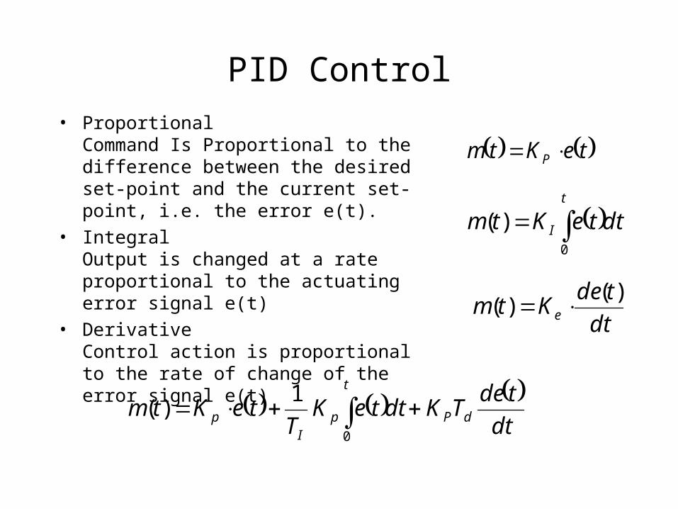
PID Control

• ProportionalCommand Is Proportional to the difference between the desired set-point and the current set-point, i.e. the error e(t).

• IntegralOutput is changed at a rate proportional to the actuating error signal e(t)

• DerivativeControl action is proportional to the rate of change of the error signal e(t)

teKtm P

dtteKtmt

I0

)(

dt

tdeKtm e

)()(

dt

tdeTKdtteK

TteKtm dP

t

pI

p 0

1)(

PID Control• Proportional

– Is an amplifier with an adjustable gain

• Integral– Removes Steady state error.

– Can destabilize a system

• Derivative– Has an anticipatory action

– Amplifies noise in the signal

– May cause saturation in the actuator.

– Why can it not be used alone.

e m-+

Feed Forward• Predict what command should be used in advance• Requires model of the system

– Can Cause instability if model is not good– Calculate in Real-Time– Lookup Table (Gain Scheduling)

• Reduces following error• Allows lower system Gain

– Better Tracking– Better Stability

CommandActual Position Desired Position

Feedback

Feed forward

Plante m

-+

Model

++Command Output

Torque Loop

• Simplest Control of Motor– Torque Amplifier

– Control Force out of motor• Independent of Speed

• Independent of Position

E Current-+

Am

pmotor

Command

Load

Control of Robots

Level of Control

• Cartesian– Linear

– Model Based

• Joint

• Servo

Types of Control

• Open Loop– No feedback

• Steppers

– No disturbance rejection

• Closed Loop– Linear

– Non-linear• Adaptive

• Cartesian de-coupling

Vocabulary

• Linear: Based on linear differential equations.

• Open Loop:

• Closed Loop:

•

Open Loop Joint and Robot Control

Trajectory Generator

Control System

tθ d

tθ d

tθ d

τ

• Needs Perfect model

• No disturbance rejection

• Hope it follows Path

• Stepper motors would be an example

Closed Loop Joint Control Open Loop Robot

Trajectory Generator

Control System

tθ d

tθ d

tθ d

θ

θ

τ

• Trajectory is a function of only the desired trajectories

• Common in some industries

• If we have good model and no disturbances we get good following

Closed Loop Cartesian Control

Coordinate Conversionand

Control System

θ

θ

τ

Kinematics

dX -

+

X

• Closes loop along the path.

X

Variant of Closed Loop Cartesian Control

Control System

θ

θ

θ

τ

Kinematics

1JdX -

+

X

• Closes loop along the path.

• Errors must be small for Jacobian to work

Comparison Between Joint and Cartesian Control

• Computationally complex

• Rejects Disturbances at joints and along path

• Can follow Straight Lines and Complex trajectories

• Inverse and Direct Kinematics need to be performed.

• Errors in model may limit gains

• Simple

• Rejects Disturbances only at Joint

• Follows Joint Profile, will have not necessarily limit path error.

•

Cartesian Joint