inverse analysis to determine hygrothermal properties...

Figure 7 appea

Journal of CO

Inverse Analysis to DetermineHygrothermal Properties in Fiber

Reinforced Composites

PAVANKIRAN VADDADI,* TOSHIO NAKAMURA AND RAMAN P. SINGH

Department of Mechanical Engineering, State University of

New York at Stony Brook, NY 11794, USA

(Received August 26, 2005)(Accepted December 9, 2005)

ABSTRACT: Fiber-reinforced composite laminates are often used in severeenvironments such as high temperature and humidity conditions. Therefore, it isof practical interest to establish a simple but robust method to determine materialproperties that define the hygrothermal behavior of composites under variousconditions. In this article a novel inverse analysis approach is presented to identifythe diffusivity, maximum moisture content, and coefficient of thermal expansion(CTE) and coefficient of moisture expansion (CME) of carbon fiber-reinforcedepoxy matrix composites subjected to various conditions of environmental exposure.This procedure involves three distinct steps. First, the transient expansions andweight gains are experimentally measured under different temperatures and humidityconditions. Next, reference solutions are established from detailed computationalmodels, which incorporate the heterogeneous nature of composite’s microstructure.Finally, the Kalman filter technique is utilized to extract best estimates of thematerial parameters of interest. The use of inverse analysis is necessitated by the factthat backward relations from the measured parameters to the unknown propertiesare not directly apparent. The results show diffusivity to be a strong functionof temperature while the maximum moisture content to be a strong functionof relative humidity. For the case of material expansion, moisture inducedstrains as well as thermal strains exhibit slight dependence on temperature.In addition to estimating the material parameters of interest, detailed studies areconducted to investigate the source of scatterings observed in the expansionmeasurements during heating and moisture absorption, and possible 3D effects inmeasurements.

KEY WORDS: moisture diffusivity, moisture content, moisture expansion, thermalexpansion, Kalman filter, fiber optic sensors.

*Author to whom correspondence should be addressed. E-mail: [email protected]
rs in color online: http://jcm.sagepub.com
MPOSITE MATERIALS, Vol. 41, No. 3/2007 309

0021-9983/07/03 0309–26 $10.00/0� 2007 SAGE

DOI: 10.1177/0021998306063372
Publications

INTRODUCTION

CARBON FIBER-REINFORCED EPOXY matrix composites are used extensively inaerospace and other structural applications because of their high strength, high

stiffness, and low density. However, harsh environmental conditions can cause deleteriouseffects on the mechanical properties and residual strength of these materials. Under hightemperature and humidity, the composites undergo various thermophysical changes.Exposure to humidity causes moisture absorption and dilatational expansion in thepolymer matrix. A large mismatch in the hygrothermal strains between the matrix andthe fibers can generate large internal stresses which may affect gross performance of thecomposite [1]. Other studies [2–4] have also indicated that moisture absorption leadsto changes in chemical characteristics of the epoxy matrix by plasticization and hydrolysis.Such effects are enhanced by concurrent exposure to ultraviolet (UV) radiation [5].Hygrothermal exposure can lower both the elastic modulus and the glass transitiontemperature of polymer matrix [4,6–8]. Degradation can also lead to moisture wickingalong the fiber–matrix interfaces, which reduces structural integrity. The major mechanicaleffects of environmental degradation are the deterioration of matrix-dominated propertiessuch as compressive strength (lower critical loads for buckling and kink band formation),weakened interlaminar bonding in cross-plies, and lowered fatigue resistance andresidual impact tolerance [2,6,7,9,10].

Several investigations have focused on the synergistic effects of moisture andtemperature on the mechanical properties and durability of composites. Asp [11] studiedthe effects of these conditions on interlaminar delamination. The durability of graphite-epoxy composites under combined hygrothermal conditions was also investigated [12]and the accumulation and progression of fatigue damage was found to depend on theenvironment. Choi et al. [8] reported on the effects of fiber volume fraction, void fraction,and ply orientations on the moisture absorption rate of carbon-epoxy fiber composites.They noted that the moisture absorption behavior is affected by the temperature history,and that the diffusivity increases with matrix volume fraction and void fraction.These studies illustrate the importance of hygrothermal behavior in determining thedurability and residual strength of composites subjected to environmental exposure. Themoisture diffusion process can be characterized by the diffusivity and the maximummoisture content while the deformation due to moisture absorption or temperatureis characterized by coefficient of moisture (CME) and coefficient of thermal expansion(CTE), respectively.

The objective of the current work is to evaluate a novel inverse analysis approachto determine the hygrothermal parameters of fiber-reinforced composites. Theseparameters are normally functions of the environmental exposure conditions(i.e., temperature and relative humidity). Loos and Springer [13] found that the maximummoisture content is a strong function of the relative humidity of the exposure environmentwhile the diffusivity is a strong function of the temperature. In general, the maximummoisture content is determined by exposing the material to a given relative humidity fora sufficiently long time until the limiting saturation is attained and the specimen doesnot absorb moisture any further. Obviously, this process is time consuming and oftencumbersome. In the proposed procedure, the test duration can be shortened significantlyby extrapolating the maximum moisture content from the record of transient moistureabsorption measurements.

310 P. VADDADI ET AL.

In general, effective or averaged properties are used to characterize the overall behaviorof composites. Such properties may be obtained either with a rule-of-mixtures approachor by numerical analyses. While the use of effective properties is appropriate for steady-state conditions, their applicability for transient conditions is, at best, questionable.More specifically, under transient conditions, the effective properties do not describe thetime and spatial variations of the parameters of interest accurately (e.g., local moisturecontent).

Previously, we have estimated the diffusivity and the maximum moisture content usingexperimental measurements of relative weight gain for composite specimens exposedto hygrothermal conditions [14]. In the present investigation, to estimate additionalparameters (i.e., the CTE and CME), weight as well as expansion were measured.Furthermore, an appropriate inverse analysis algorithm was established to accommodatethe multiple measurements as well as the increased number of unknowns. In the tests,expansions due to moisture absorption and temperature variation were recorded usingfiber-optic strain sensors. These sensors offer numerous advantages over conventionalresistive foil strain gages through increased resolution and accuracy, insensitivity toelectromagnetic interference and the capability of use at high temperature and moistureconditions. In recent years, fiber-optic sensors have been increasingly used for strainmeasurements in composites due to their small size and ability to be embedded or bondedinside the material [15–17]. In the present experiments, the primary advantage of fiber-optic strain sensors, over more conventional stain gages, is not only their insensitivity tothe electromagnetic noise inside the environmental chamber but also their long-termdurability in harsh environments.

Since the response times of moisture transport and thermal expansion are very different,two separate tests were conducted to quantify the parameters. First, in order to measurethe moisture absorption behavior, specimens were placed in an environmental chamberfor up to 1200 h (50 days) under various humidity and temperature conditions. To measurethe CTE, specimens were kept in the chamber for much shorter durations (i.e., minutes).Since the thermal equilibrium is reached several orders of magnitude faster than themoisture saturation, the transient thermal parameters (e.g., thermal conductivity) ofcomposites were not determined here. On the other hand, the transient characteristicsof moisture flow are very important, and thus the diffusivity, CME, and the maximummoisture content were estimated under various temperatures and humidity conditions,as they were considered to be functions of temperature and humidity. Theintegrated experimental and inverse analysis approach employed in this investigation isdescribed next.

EXPERIMENTAL PROCEDURE

Composite Specimen

Specimens were machined from commercially fabricated laminates of IM7/997 carbon-fiber reinforced epoxy donated by Cytec Engineered Materials, Inc. (Anaheim,California). This composite is under development for application to aerospace andexpected to provide higher damage tolerance than currently qualified materials such asIM7/5271-1 [18]. These laminates consist of PAN based, 5 mm diameter IM7 carbon

Inverse Analysis to Determine Hygrothermal Properties 311

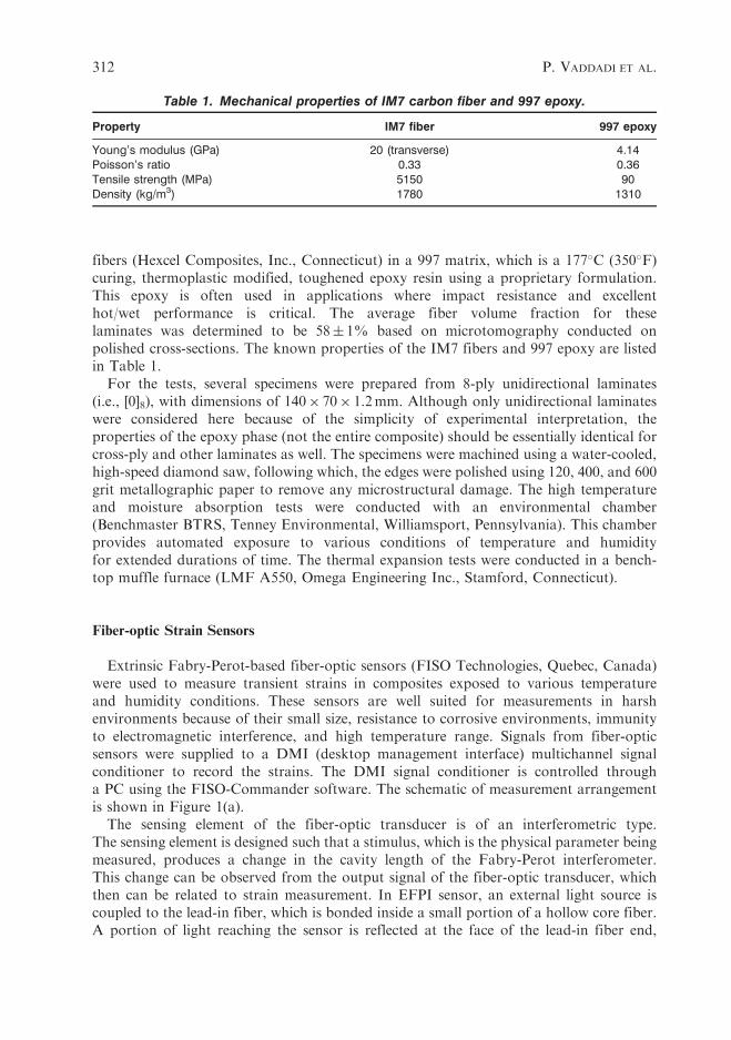
fibers (Hexcel Composites, Inc., Connecticut) in a 997 matrix, which is a 177�C (350�F)curing, thermoplastic modified, toughened epoxy resin using a proprietary formulation.This epoxy is often used in applications where impact resistance and excellenthot/wet performance is critical. The average fiber volume fraction for theselaminates was determined to be 58� 1% based on microtomography conducted onpolished cross-sections. The known properties of the IM7 fibers and 997 epoxy are listedin Table 1.

For the tests, several specimens were prepared from 8-ply unidirectional laminates(i.e., [0]8), with dimensions of 140� 70� 1.2mm. Although only unidirectional laminateswere considered here because of the simplicity of experimental interpretation, theproperties of the epoxy phase (not the entire composite) should be essentially identical forcross-ply and other laminates as well. The specimens were machined using a water-cooled,high-speed diamond saw, following which, the edges were polished using 120, 400, and 600grit metallographic paper to remove any microstructural damage. The high temperatureand moisture absorption tests were conducted with an environmental chamber(Benchmaster BTRS, Tenney Environmental, Williamsport, Pennsylvania). This chamberprovides automated exposure to various conditions of temperature and humidityfor extended durations of time. The thermal expansion tests were conducted in a bench-top muffle furnace (LMF A550, Omega Engineering Inc., Stamford, Connecticut).

Fiber-optic Strain Sensors

Extrinsic Fabry-Perot-based fiber-optic sensors (FISO Technologies, Quebec, Canada)were used to measure transient strains in composites exposed to various temperatureand humidity conditions. These sensors are well suited for measurements in harshenvironments because of their small size, resistance to corrosive environments, immunityto electromagnetic interference, and high temperature range. Signals from fiber-opticsensors were supplied to a DMI (desktop management interface) multichannel signalconditioner to record the strains. The DMI signal conditioner is controlled througha PC using the FISO-Commander software. The schematic of measurement arrangementis shown in Figure 1(a).

The sensing element of the fiber-optic transducer is of an interferometric type.The sensing element is designed such that a stimulus, which is the physical parameter beingmeasured, produces a change in the cavity length of the Fabry-Perot interferometer.This change can be observed from the output signal of the fiber-optic transducer, whichthen can be related to strain measurement. In EFPI sensor, an external light source iscoupled to the lead-in fiber, which is bonded inside a small portion of a hollow core fiber.A portion of light reaching the sensor is reflected at the face of the lead-in fiber end,

Table 1. Mechanical properties of IM7 carbon fiber and 997 epoxy.

Property IM7 fiber 997 epoxy

Young’s modulus (GPa) 20 (transverse) 4.14Poisson’s ratio 0.33 0.36Tensile strength (MPa) 5150 90Density (kg/m3) 1780 1310


while the rest travels through the air gap and is partially reflected at the fiber end. Thelight reflected back from the two surfaces is transmitted back to the lead-in fiber anddeformation can be measured from the change in gap length. The free end of the sensoris connected to the DMI conditioner, as shown in a schematic of the sensor operationin Figure 1(b). The conditioner samples the transducer signal at a fixed rate of 20Hz, andthe readings are averaged for a given period of time and stored as measured records.For each specimen, two sensors (one on each surface) were bonded transversely withrespect to the carbon fiber direction as illustrated in Figure 1(a). Here, only the transverseor normal strain perpendicular to the fiber direction was measured because of its greaterexpansion. An accessory hole in the environmental chamber allowed for strainmeasurements to be conducted during the environmental exposure. Although the currenttest placed the sensors on the free surfaces, fiber-optic sensors can be also embeddedwithin the composites during their fabrication process. Then the proposed inverse analysis

Hollow core tube

Single mode fiber Multi mode fiber

(a)

(b)

DMI conditioner

PC

Case D

Environmentalchamber

Figure 1. (a) Schematic of data acquisition system to measure strain of specimen in environmental chamber.(b) Illustration of the fiber optic sensor.


can readily accommodate such internal strain measurements to estimate the unknownproperties.

Bonding of the fiber-optic sensors required special care due to their small size and highsensitivity. First, the specimen surface was cleaned with acetone followed by dry and wetabrasion with sand paper. The fiber-optic gage was then held onto the specimen withan electric tape in the desired orientation and a 5-min epoxy was used 3mm from thegage-sensitive region to ensure proper alignment with specimen. Subsequently, theadhesive was applied, taped, and allowed to cure. To adhere the fiber-optic sensor tothe surface, it was shielded with a thin epoxy layer (�100 mm thick). These steps followthe procedure recommended by FISO technologies. Although, the thickness of the extralayer is small, it may still act as a barrier to moisture absorption and consequently alterexpansion characteristics of composites. In order to quantify its effect, a detailedcomputational analysis was carried out and described in the Appendix. The analysisessentially confirms such an effect to be minimal and that it does not influence theestimations of unknown parameters.

Weight Measurements

Another measurement parameter was the weight gain of composites due to moistureabsorption under various environmental conditions. For each exposure condition, theweight gain was monitored for two nominally identical specimens placed in theenvironmental chamber. These specimens were additional to those used for monitoringstrains with fiber-optic sensors. The separate specimens were necessary due to difficultyin measuring the weights of specimens with fiber-optic sensor attached. During the tests,two specimens were taken out of the chamber every 24 h. The surfaces were dried carefullyand the weights were measured using an analytical balance with a resolution of 0.1mg,which corresponds to �5� 10�4% of the specimen weight. After they were weighed,the specimens were immediately placed back in the chamber. The entire process required�5min. It should also be noted that all specimens were preconditioned at 50�C for2 weeks until no change in weight was observed. This process ensures that the specimensare uniformly dry prior to environmental exposure.

Moisture Absorption Tests

In order to determine the individual effects of relative humidity (RH) and temperature(T ), four separate environmental conditions were considered:

Case A : T ¼ 85�C and RH ¼ 85%,

Case B : T ¼ 40�C and RH ¼ 85%,

Case C : T ¼ 85�C and RH ¼ 50%, and

Case D : T ¼ 40�C and RH ¼ 50%:

These conditions encompass a range of hygrothermal environments of interest. Inthe analysis, it was assumed that moisture absorption occurs only in the epoxy matrixand not in the carbon fibers. For each environmental condition, the chamber was allowed


to stabilize and the strain sensors were initialized to eliminate any effects of expansiondue to the temperature.

The normalized weight gain and transverse strain (perpendicular to fibers) measure-ments for the four environmental conditions are shown in Figure 2. The normalizedweight change is obtained by dividing the increase in weight by the initial dry weight ofspecimen. For the lower temperature tests (Cases B and D), the specimens were kept inthe chamber for 1200 h (50 days) while for the high temperature tests, (Cases A and C),the specimens were kept in the chamber for about 600 h (25 days). For each condition,

(a)

(b)

Time (h)

0 200 400 600 800 1000 1200

Nor

mal

ized

wei

ght g

ain

(%

)

0.0

0.1

0.2

0.3

0.4

0.5

0.6

Environmental conditions

T = 85°C, RH = 85%T = 40°C, RH = 85%T = 85°C, RH = 50%T = 40°C RH = 50%

Case A

Case B

Case C Case D

Time (h)

0 200 400 600 800 1000 1200

Str

ain

(×10

−3)

0.0

0.2

0.4

0.6

0.8

1.0

1.2

1.4


T = 85°C, RH = 85%T = 40°C, RH = 85%T = 85°C, RH = 50%T = 40°C, RH = 50%

Case A

Case B

Case C Case D

Figure 2. Experimental measurements of: (a) weight gains due to moisture absorption and (b) transversestrains due to moisture expansion, shown as functions of time under different environmental conditions.


the plots show average values obtained from two separate specimens. Typical differencesin the normalized weight changes of two specimens were �1%. Similarly, the fiber-opticstrain measurements on the top and bottom surfaces of any given specimen differedby less than 1%.

For Case A (T¼ 85�C and RH¼ 85%), a rapid increase in both weight gain and strainwas observed during the initial periods of exposure, followed by slower changes. This wasexpected as the kinetics of diffusion is driven by the absorbed moisture gradient, which ishigh during the initial phases and reduces as the specimen saturates. When the temperaturewas lowered to T¼ 40�C while keeping the RH fixed at 85% (Case B), a longer time wasneeded to achieve the saturation. Nevertheless, for both Cases A and B, the specimensappeared to approach similar limiting values (full saturation), respectively. In contrast,when the RH was lowered to 50% while maintaining the temperature at T¼ 85�C (Case C),the composite required similar time to reach the saturation but at a lower level ascompared to Case A. When both T and RH were lowered to T¼ 40�C and RH¼ 50%,respectively (Case D), again a longer time was needed to saturate for both weight gainand strain.

In Figure 2, one can also observe that the measurement curves are not smooth.For weight change, these variations may be explained by the manual wiping of specimensprior to the weighing that can introduce small error. On the other hand, smoothervariations were expected for the strain measurements since the specimens were untouchedand kept in the chamber throughout the tests. The cause of discontinuous strain changeis closely analyzed in conjunction with the thermal cycle tests presented in the ‘ThermalExpansion’ section.

Thermal Expansion Tests

The thermal expansion of composite specimens was measured over a 20–120�Ctemperature range. Composite specimens were exposed to various temperatures and thesurface strains were monitored using fiber-optic sensors. Two gages were bonded on thetwo surfaces of the composite specimen in order to ensure the measurement accuracy.To check for consistency, metal strain gages were also bonded onto the specimen.In addition, a separate aluminum plate with strain gages was placed in the sameenvironmental chamber to further monitor the testing environments.

Initially, the specimens were placed in the chamber at 20�C and the temperature wasincrementally raised up to 120�C in about 20min. At each temperature, the system wasallowed to stabilize for about a minute. The temperature was measured by an independentthermocouple in the chamber. In order to ensure the accuracy of the strain measurements,at the end of the test, the temperature was again lowered to room temperature andsubsequently raised directly to intermediate values, allowed to stablize and the strainswere compared with the earlier measurements.

The measured thermal strains of composites are shown as a function of temperaturein Figure 3. Note that the thermal strain of aluminum plate essentially increased linearlywith the temperature, assuring the accuracy of the testing condition. As observed in thefigure, the strain changes of composite were highly uneven during the first heating (note:these are from virgin specimens). At first, the cause was thought to be the inhomogeneousnature of composite microstructure. However as the thermal tests were repeated, a lesserscattering was observed in the measurements. In fact, at the ninth heating cycle, the strain


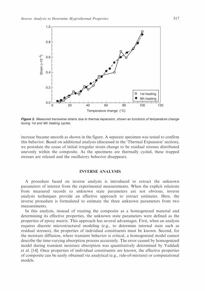
increase became smooth as shown in the figure. A separate specimen was tested to confirmthis behavior. Based on additional analysis (discussed in the ‘Thermal Expansion’ section),we postulate the cause of initial irregular strain change to be residual stresses distributedunevenly within the composite. As the specimens are thermally cycled, these trappedstresses are relaxed and the oscillatory behavior disappears.

INVERSE ANALYSIS

A procedure based on inverse analysis is introduced to extract the unknownparameters of interest from the experimental measurements. When the explicit relationsfrom measured records to unknown state parameters are not obvious, inverseanalysis techniques provide an effective approach to extract estimates. Here, theinverse procedure is formulated to estimate the three unknown parameters from twomeasurements.

In this analysis, instead of treating the composite as a homogenized material anddetermining its effective properties, the unknown state parameters were defined as theproperties of epoxy matrix. This approach has several advantages. First, when an analysisrequires discrete microstructural modeling (e.g., to determine internal state such asresidual stresses), the properties of individual constituents must be known. Second, forthe moisture diffusion, where transient behavior is critical, a homogenized model cannotdescribe the time-varying absorption process accurately. The error caused by homogenizedmodel during transient moisture absorption was quantitatively determined by Vaddadiet al. [14]. Once properties of individual constituents are known, the effective propertiesof composite can be easily obtained via analytical (e.g., rule-of-mixture) or computationalmodels.

Str

ain

(×10

−3)

Temperature change (°C)

0 20 40 60 80 100 1200.0

0.2

0.4

0.6

0.8

1.0

1st heating 9th heating

Figure 3. Measured transverse strains due to thermal expansion, shown as functions of temperature changeduring 1st and 9th heating cycles.


It should be also noted that one may opt to seek these parameters from bulk epoxy.However, in many instances, same particular epoxy is not available in bulk form, andalso the curing process during composite fabrication may not produce identicalproperties. In addition, the present procedure also allows for the testing of agedcomposites to determine their modified moisture transport characteristics. Anotheradvantage of directly determining epoxy properties of already fabricated composite isthat it considers other effects such as small voids/cracks introduced during processing,and possible decohesion at fiber–matrix interfaces. These process-induced effects areimplicitly included in the estimated properties of epoxy, and thus are more suitablein modeling of matrix–fiber composites.

In the current study, the unknown parameters are the maximum moisture content,C*, the diffusivity, D, the coefficient of moisture expansion (CME), �, and the CTE, � ofthe epoxy matrix. The last parameter is determined independently from the thermal test.Since the carbon fibers absorb very little moisture, their diffusivity, maximum moisturecontent, and coefficient of moisture expansion were assumed to be zero. The CTE ofcarbon fibers was treated as known since its value is well documented. For the inverseanalysis technique we employ the Kalman filter, which has been widely used in many areasof engineering, such as sensor calibration, tracking applications, trajectory determination,and image and signal processing [19–22]. It has been also used for the estimation of variousunknown material parameters [23–25]. The main advantage of the Kalman filter algorithmover other adaptive algorithms is that it is highly effective in nonlinear systems and hasa fast convergence to optimal solutions. In addition, due to its mathematical structure,it has the ability to filter out measurement noise and error. These properties makethe technique ideally suited for the present investigation since the moisture absorptionprocess is nonlinear with time, and the measurements can contain some errors. Prior toimplementing this technique, it must be carefully tailored and adopted to the presentanalysis, as described next.

Kalman Filter Procedure

In the Kalman filter formulation, the three unknown parameters are denoted in a vectorform as Xt¼ (C�

t , Dt, �t)T, where C�

t , Dt, and �t are the current estimates of the maximummoisture content, diffusivity, and coefficient of moisture expansion of epoxy, respectively.Here t may represent the actual time as well as a pseudotime such as a step/incrementnumber that ranges 0� t� tmax. The successive estimates are indirectly made from themeasured weight gain, wmeas

t , and moisture induced strain, "meast , which may contain error/

noise as wmeast ¼wtþwerr

t , and "meast ¼ "tþ "errt , respectively. At t¼ 0, the initial estimates

C�o, Do, and �o are assigned and the subsequent estimates are made according to the

following algorithm.

Xt ¼ Xt�1 þ Kt Mmeast �Mt Xt�1ð Þ

� �: ð1Þ

Here, Kt is the ‘Kalman gain matrix’ and Mmeast is a vector containing measured record

of weight gain wmeast and the strain "meas

t (i.e., Mmeast ¼ wmeas

t , "meast )T) at t. Also Mt(Xt�1)

is a vector containing measured parameters computed with estimated unknown stateparameters at the previous step. Note that these computations require solutions of


measured parameters for a given set of state parameters. Such solutions are sometimesreferred as the ‘forward’ solutions. In the above equation, the Kalman gain matrixmultiplies the difference between the measured and computed values of the weight gainand strain to make corrections to the unknown state parameters. The Kalman gain matrixis computed as

Kt ¼ PtM0Tt R

�1t where Pt ¼ Pt�1 � Pt�1M

0Tt M0

tPt�1M0Tt þ Rt

� ��1M0

tPt�1: ð2Þ

With three state and two measured parameters, the dimensions of Kalman gain matrixare 3� 2. Also M0

t is a 2� 3 matrix that contains the gradients of Mt with respect to thestate parameters C*, D, and � as

M0Tt ¼

@Mt

@X¼

@wt

@C�

@wt

@D

@wt

@�@"t@C�

@"t@D

@"t@�

0BB@

1CCA: ð3Þ

In addition, Pt is the ‘measurement covariance matrix’ related to the range of unknownstate parameters at increment t, and, Rt is the ‘error covariance matrix’, related to the sizeof measurement error. Once the initial values are imposed, Pt is updated every step, whileRt is prescribed at each step. However, in many cases, fixed values can be assigned to thecomponents of Rt as long as measurement error bounds do not vary substantially duringthe duration of measurements. Since the convergence rate is sensitive to the values ofPt and Rt, proper assignments for these two matrices are essential. After several trials,the initial measurement covariance matrix and the constant error covariance matrix wereassigned in this analysis as

Po ¼

�C�ð Þ2 0 0

0 �D�ð Þ2 0

0 0 ��ð Þ2

24

35 and Rt ¼

10Rw 00 10R"

� �: ð4Þ

Here �C*, �D, and �� denote the expected ranges of the unknown parameters,respectively. While Po is diagonal, the procedure results in a filled Pt matrix duringsubsequent increments. In the current analysis, the diagonal components of Rt are chosenbased on the estimated measurement error for the weight and the strain measurements.Here 10Rw and 10Rs denote 10 times the normalized estimated maximum errors of theweight and strain measurements. Based on the experimental measurements, as shownin Figure 2, dimensionless Rw and Rs were estimated as 2� 10�3 and 8� 10�3, respectively.In general, larger values lead to slower but stable convergence to the solutions of unknownstate parameters. The Kalman filter procedure, which is summarized in Figure 4, wasimplemented in a computational code.

As noted earlier, the Kalman filter requires the solutions of weight gain wt, strain "t, andtheir gradients w0

t and "0t for given values of C*, D, and � at a given time (i.e., forwardsolutions). For some problems, these solutions may be obtained from closed-formanalytical solutions or simple numerical calculations. However, in many cases involvingcomplex boundary and geometrical conditions, the solutions can be obtained only throughseparate analyses. For moisture diffusion problems, they can be approximated using the


Fickian equation in a homogenized model without resorting to detailed computations.Such a procedure, however, was found to be inaccurate for transient moisture transportin composites, as previously discussed. Thus, detailed finite element simulations werecarried out for the moisture absorption process to generate accurate functions for wt, "t,w0t, and "0t, as discussed in ‘Finite Element Simulations’.

Reference Data and Domain of Unknowns

The Kalman filter algorithm requires time-varying solutions of weight gain and strainas functions of the unknown state parameters. As no simple solutions are available,which explicitly account for the heterogeneous constitution of composites, finite element

Set t = 0Assign initial estimates

Xo = (Co*, bo, Do)T

(state vector containingunknown parameters)

Set t = t + 1

Set Xest= Xt

Check t = tmax

Yes

No

Read in measured Mtmeas at increment t

Where, Mtmeas = (wt, εt )

Update Xt = (Ct*, bt, Dt)T as

Xt = Xt−1 + Kt [Mtmeas – Mt(Xt−1)]

Compute Kalman Gain Matrix

Kt = Pt M't TRt

−1

where matrix of covariance (of estimated Xt) is

Pt = Pt-1 – Pt−1M'tT

(M't Pt−1M'tT +Rt)

−1 M't Pt−1

and gradient of weight gain wrt to C*, D, and b is

∂X

∂M(Xt−1)M't =

Figure 4. Flowchart for Kalman filter to estimate maximum moisture content, diffusivity, and coefficient ofmoisture expansion from time history measurements of strain and weight gain.


simulations were carried out to establish the reference data or forward solutions.The reference data comprise of time-dependent variations of strain, weight gain, andtheir gradients for various values of C*, D, and �.

Prior to determining the reference solutions, it is necessary to set bounds or a domainfor the unknown parameters. The required domain can be approximated either fromavailable information regarding the unknown state parameters or from comparison ofthe experimental measurements and results of a few trial simulations. Here, bothapproaches were used to select the domain for the maximum moisture content C*,diffusivity D, and coefficient of moisture expansion �. A schematic of three dimensional(3D) domain is shown in Figure 5, where the values were set as 0.57%�C*� 2.27%,10� 10�14m2/s� D� 75� 10�14m2/s, and 0.25� 10�3/%�� 2.5� 10�3/%, respec-tively. The unit of C* is weight percent of water (H2O), and the unit of � is per weightpercent of H2O. Since computations with many different sets of state parameters wouldbe prohibitive, we utilized cubic Lagrangian interpolation functions. Here sixty-four(¼ 4� 4� 4) base points were chosen and the finite element simulations were performedfor specified sets of C*, D, and �. At each set of state parameters, solutions of weightand strain were stored for every 24-h time increment. When wt and "t at anyintermediate values of C*, D, and � were required, they and their gradients wereinterpolated with the cubic Lagrangian functions. This approach was found to bevery accurate as long as the measured parameters were sufficiently smooth functions ofthe state parameters.

Finite Element Simulations

In the finite element analysis, we capture the heterogeneous microstructure usingrandomly distributed fibers to model the fiber-reinforced composite. The motivation to

D (×10−14m2/s)

C* (%)

b (×10−3/%)

0.25

75

10

2.50

2.270.57

Domain of unknownparameters

Figure 5. Domain of unknown state parameters shown in 3D space defined by maximum moisture contentC*, diffusivity D, and moisture expansion coefficient �. Best estimates are explored within the domain.


adopt such a model was threefold. First, a homogenized model does not simulate accuratetransient behavior of moisture diffusion as described previously. Detailed comparisonstudy with 1D Fickian model is shown in [14]. Second, unit cell models, popular in manycomposite analyses, cannot be used here since the moisture transport occurs acrossthe entire thickness. Third, again due to the transient nature of the problem, modelswith regularly spaced fibers (e.g., hexagonal packing) do not offer sufficiently accuratesolutions. Thus, the random nature of fiber distributions is essential in capturingcharacteristics of transient moisture transport in the fiber-reinforced composites(as discussed in detail in [14]). These conditions led us adopt the random fiber modelthat has good resemblance to the microstructure of actual specimens.

The specimen has eight plies totaling a thickness of 1.2mm. Figure 6(a) shows thegeometric model of the composite specimen and the considered section. Due to thesymmetry across the center-plane, only one-half thickness of the composite is modeled.The effects of edges can be effectively ignored since the total area of the front/backsurfaces is much greater than the edge area (by a factor of 37). This reduces the problemto be two-dimensional (2D). In the analysis, both the moisture absorption as well as theexpansion due to the moisture was considered. The fibers were placed randomly withinthe domain with a computational code. Special algorithms were required to positionfibers beyond a volume fraction of 50% since the space available to place extra fibersdiminishes greatly. The program rearranges the initially placed fibers to optimize theavailable space and then restarts to place fibers in the modified configuration. This processis repeated until the desired volume fraction is achieved. The model width is set to 64 mm,which has about 10 fibers distributed across. The final model contains about 1200 fibers,totaling the given fiber volume fraction of 58%.

Once the random fiber geometric model was created, a mesh generator code was utilizedto construct the finite element mesh shown in Figure 6(b) and (c). The element sizes werekept sufficiently small for accurate simulation of transient moisture transport anddeformation analysis. The entire mesh contains more than 130,000 nodes and 240,000triangular generalized plane strain elements. Although detailed convergence analysis wasnot possible due to mesh complexity, two additional meshes with different random fiberdistributions were constructed to check for the consistency. The solutions from the threemodels showed essentially identical results.

The transient moisture induced deformation was studied in a coupled temperature–displacement analysis of the finite element analysis [26]. The analogy between Fick’s lawfor mass diffusion and Fourier’s law for heat transfer was employed to model transientmoisture diffusion [27]. The values of conductivity, specific heat, and density, for a heattransfer analysis, were adjusted appropriately to provide solutions for transient moisturediffusion. For the boundary conditions, symmetry conditions in moisture, displacement,and temperature were imposed along the sides of the model except along the exposedsurface. For the symmetry conditions, the three sides were kept straight and the fourcorners were set to remain perpendicular to represent an infinitely wide laminate For thefinite element model, moisture flows only across the top surface exposed to the humidity.Thus, it was possible to specify the maximum moisture content for given environmentalconditions as the boundary condition on this surface. At time t¼ 0, the entire specimenhad zero moisture content. For t>0, a fixed level of moisture condition is imposed alongthe top for each condition. The computational analysis of moisture diffusion was carriedout over the respective duration of experimental tests (either 600 or 1200 h). As the mois-ture is transported and absorbed through the specimen, the total weight increases and the


epoxy phase undergoes dilatational expansion. The total weight gained by the specimenwas obtained by numerically integrating moisture content of all elements every 24 h.

Moisture absorption and temperature change result in stresses associated withhygrothermal expansion in the composites. The linear constitutive relationship for theepoxy can be shown as

�ij ¼ �"kk�ij þ 2�"ij � ð3�þ 2�Þ ��Cþ ��Tð Þ�ij, ð5Þ

(c)

(b)

(a)

Surfaces directly exposedto environmentSymmetry plane

t = 1.2mm

Half-thicknessmodel

Figure 6. Schematics of random fiber model used in the finite element transient analysis: (a) physical model;(b) outlines of 1200 fibers in the half-thickness model; and (c) enlarged view of mesh with fibers.


where � and � are the Lame constants. Although not shown, our computational resultsestimated that the internal stresses to reach as high as 50MPa in tension at certainlocations where multiple fibers are clustered. These high stresses can initiate matrixcracking and debonding of the matrix and fibers.

ESTIMATION OF HYGROTHERMAL PROPERTIES

Transient Moisture Absorption

The best estimates of moisture-related material parameters were extracted using theKalman filter with available measurements and reference data. The Kalman filter is basedon an incremental approach and updates the estimates with the measured weight andstrain that were provided at every time increment. At the first increment, initial estimatesof unknown parameters must be assigned. In general, the final converged estimates arenot identical for different initial estimates. In our unique procedure to identify the bestestimates, the Kalman filter was carried out with many different initial estimates of C*, D,and � with their values spread evenly (at 40� 40� 40 points) in their domain of unknowns(Figure 5). For each set of initial estimates, the Kalman filter computed the final estimates.In order to illustrate different locations of final estimates, contour plots were constructed.These intensity of convergence plots can then be used to identify most likely values ofbest estimates. A location with high contour value signifies that more initial estimatesconverged near the particular values of C*, D, and �. Thus best estimates can be takenat the highest intensity of convergence.

The results of Kalman filter for different environmental conditions are shown inFigure 7. Here, the contour values are normalized so that the highest intensity takesthe value of 100. Although three unknowns were estimated simultaneously, their intensityof convergence is shown in two separate 2D plots for clarity. Here, in each plot,convergence intensity of two out of the three parameters is shown. Although another plotwith the remaining combination is available, it is not shown to save space. Figure 7(a)shows the results of Case A with T¼ 85�C and RH¼ 85%. For this case, the best estimatesof the unknown state parameters were identified as C*¼ 1.45%, D¼ 54.3� 10�14m2/s,and �¼ 1.89� 10�3/%, respectively. Note the highest intensity was determined from allthree parameters and it may not necessarily coincide with that of the two parameter plotsshown in the figures. Similar convergence results were obtained for the other three casesas shown in Figure 7(b), (c), and (d), respectively. The summary of best estimates forvarious environmental conditions is presented in Table 2. These results clearly exhibit theirdependence on the relative humidity and/or temperature. The most significant influenceis observed in the temperature dependence of diffusivity.

As noted earlier, the strength of inverse analysis approach lies in its ability to estimateunknowns with limited data. In order to illustrate this point, separate analyses wereperformed with shorter time durations of experimental measurements. For example,for Case A (T¼ 85�C and RH¼ 85%), only first 360 h of weight and strain measurementswere used instead of measurements over 600 h. The results of best estimates obtained withreduced experimental records are shown in Table 3. Although differences in the estimatescan be observed in each case, they are generally within 5% of the estimates made with thefull measurements shown in Table 2. For Cases B and D, the reduction in time periodis 480 h (20 days), which represents significant savings in the long-term tests. These results


demonstrate that the present method is effective in estimates unknowns with dataonly from transient stage. This feature is particularly attractive for lower temperaturetests when complete saturation can take much longer times.

In most inverse problems, there is no independent way to prove the best estimatesare indeed close to the correct solutions. However, there are two ways to assess thelikeliness of accuracy. One is from the sizes of converged regions shown in the intensity ofconvergence plots. A small region implies that the inverse method is robust since manyinitial estimates converged near the same location (i.e., similar estimates). The convergedregions shown in Figure 7 are reasonably contained, which suggests reasonable accuracyof best estimates. An additional confirmation can be made from a simulation study. Usingthe best estimates identified in the inverse analysis as the inputs, the moisture diffusionprocess can be resimulated in the finite element analysis. Then the simulated relative

Case A: T = 85°C, RH = 85%

High

Low

High

Low

Diffusivity D (×10−14 m2/s)

30 45 60 75

CM

E b

(×10

−3 /

%)

0.25

1.00

1.75

2.50

Maximum moisture content C* (%)

0.57 1.14 1.71


30 45 60 75

CM

E b

(×1

0−3 /

%)

0.25

1.00

1.75

2.50


0.57 1.14 1.71

Case B: T = 40°C, RH = 85%

High

Low

High

Low

(a)

(b)

Intensity ofconvergence Best estimates

C* = 1.45%b = 1.89×10−3 /%

Intensity ofconvergence

Best estimates

D = 54.3×10−14 m2/sb = 1.89×10−3 /%

Best estimatesC* = 1.41%b = 1.63×10−3 /%

Best estimates

b = 1.63×10−3 /%D = 13.2×10−14 m2/s



Figure 7. Results of Kalman filter for different environmental conditions.



30 45 60 75

CM

E b

(×1

0−3 /

%)

0.25

1.00

1.75

2.50


0.57 1.14 1.71

High

Low

High

Low

Case C: T = 85°C, RH = 50%

Diffusivity D (×10−14m2/s)

30 45 60 75

CM

E b

(×1

0−3 /

%)

0.25

1.00

1.75

2.50


0.57 1.14 1.71

High

Low

High

Low

Case D: T = 40°C, RH = 50%

(c)

(d)

C* = 1.08%β = 1.61×10−3 /%

C* = 1.12%β = 1.85×10−3 /%

Best estimates



Best estimates

D = 52.4×10-14 m2/sβ = 1.85×10−3 /%

D = 12.4×10−14 m2/sβ = 1.61×10−3 /%



Best estimatesBest estimates

Figure 7. Continued.

Table 2. Estimated hygrothermal parameters of epoxy based on inverse analysisfor the different environmental conditions.

Exposure conditionsDiffusivity Max. moist.

Case T (�C) RH (%) Time (h) (�10�14m2/s) content (%) CME (�10�3/%)

A 85 85 600 54.3 1.45 1.89B 40 85 1200 13.2 1.41 1.63C 85 50 600 52.4 1.12 1.85D 40 50 1200 12.4 1.08 1.61


weight gains and strain changes are compared with the actual measurements as shown inFigure 8. The agreements between the measured and simulated values are remarkable.Except near the initial phase, the simulated results are well within the bounds of measuredoscillations throughout the measured time period. Although the good agreement does notprove the uniqueness, it further supports the accuracy of parameters obtained in thepresent inverse analysis.

Thermal Expansion

As previously described, the CTE were estimated from separate tests since thermalequilibrium is achieved much faster than moisture saturation. As in the case of moistureexpansion, the normal strain perpendicular to the fiber direction was measured in thermalexpansion tests. Since strain measurements were made at discrete temperatures, the CTEof composites was determined from the difference in strains at two different temperatures,whose average is reported as the corresponding temperature. As shown in Figure 3, thestrains did not exhibit a smooth variation with increasing temperature. Consequently,the computed effective CTE of composite is highly oscillatory during the course of thefirst heating cycle as shown in Figure 9. As the specimen was reheated, changes in CTEbehavior became smoother.

This behavior is investigated here. First, to quantify the scattering at each heating cycle,an index that represents average deviation from linear fit is introduced as

s ¼1

N

XNi¼1

�measi � �fit

i

�fiti

��: ð6Þ

Here �measi is the ith temperature increment of measured CTE, N is the total measurements,

and �fiti is the CTE of linearly fitted curve (generated from all data) at the ith increment.

Note that the standard deviation was not used here since CTE is clearly dependenton temperature. The linear fit and corresponding scattering index for each specimenat selected heating cycles is also shown in Figure 9. As the specimens were repeatedlysubjected to thermal cycling, the scattering index was reduced drastically. It was alsoobserved that the linear fit equations were nearly identical for all the heating cycles.

Since repeated heating caused the scattering to subside, it was postulated that stressrelaxation occurs during the thermal cycles. Initially, the composites contain locally highresidual stresses generated during the manufacturing process. Due to the heterogeneous

Table 3. Estimated hygrothermal parameters of the epoxy based on inverse analysis usingshorter periods of experimental measurements (60% of total measured time).

Exposure conditionsDiffusivity Max. moist.

Case T (�C) RH (%) Time (h) (�10�14m2/s) content (%) CME (�10�3/%)

A 85 85 360 55.8 1.49 1.92B 40 85 720 14.1 1.44 1.69C 85 50 360 53.5 1.18 1.89D 40 50 720 13.1 1.13 1.64


nature of microstructure, thermal mismatch is likely to cause stress concentrations near thefiber–epoxy interfaces. When the specimens are heated, these stresses can cause differentdeformation state through some local microstructural changes such as interface sliding.Although the precise nature of the mechanism governing the reduction in scatter in thethermally induced strains cannot be identified within the scope of the present study, alikely phenomenon is the redistribution of residual stress and deformation fields duringcyclic heating. Note that the specimens were heated up to 120�C, which is well below theglass transition temperature of epoxy. Nevertheless, this temperature may sufficiently

(a)

(b)

0 200 400 600 800 1000 12000.0

0.1

0.2

0.3

0.4

0.5

0.6


T = 85°C, RH = 85% T = 40°C, RH = 85%T = 85°C, RH = 50%T = 40°C, RH = 50%

Case A

Case B

Case C Case D

FE simulations Measured data

Time (h)

Nor

mal

ized

wei

ght g

ain

(%

)

0 200 400 600 800 1000 12000.0

0.2

0.4

0.6

0.8

1.0

1.2

1.4


T = 85°C, RH = 85%T = 40°C, RH = 85%T = 85°C, RH = 50%T = 40°C, RH = 50%

Case A

Case B

Case C Case D

FE simulations

Measured data

Str

ain

(×10

−3)

Time (h)

Figure 8. Comparisons between measured (symbols) and computed (dash lines): (a) weight gain and(b) transverse strain. The latter solutions are obtained from finite element simulations with the best estimatesobtained in the inverse analysis.


soften epoxy to promote the redistributions. After repeated cycles, stresses are more evenlydistributed and smoother strain changes prevail.

The uneven behavior of strain observed during moisture absorption, as shown inFigure 2(b), can also be attributed to similar mechanisms. Since these phenomenaare local, it is probably difficult to detect them from overall deformation measurements(i.e., via displacement).

Once CTE of composites was determined, the CTE of epoxy was computed based onthe linear relationship obtained from the finite element calculations. Here two simulations

Temperature change (°C)

0

10

20

30

40

10

20

30

0 20 40 60 80 1000

10

20

30

0

1st heating

5th heating

Scattering index = 6.7%


9th heating


0 20 40 60 80 100

1st heating

5th heating



9th heating


Specimen 1 Specimen 2

α com

posi

te (

×10−6

/°C

)

Figure 9. Variations of CTE with temperature change shown at selected thermal cycles for two differentspecimens. The dashed line in all plots corresponds to the best linear fit obtained from the 9th heating results.


were performed with different CTE of epoxy, and the effective property of composite wasfound as �composite¼ 0.60�epoxyþ 0.40�carbon. This relation is very close to that obtainedusing a rule-of-mixtures approach. Using this relation and the linear fit of resultsduring 9th heating, the temperature dependent CTE of epoxy was determined as�epoxy¼ (0.05� 10�6/�C)�Tþ ��

epoxy, where ��epoxy ¼ 23.5� 10�6�C is the room tempera-

ture CTE. During heating from T¼ 20 to 120�C, the CTE increases by about 20%.

Summary of Hygrothermal Properties

In order to illustrate the humidity and temperature dependences of the hygrothermalproperties, the estimated parameters of epoxy under different conditions are summarizedin Figure 10. Here, the parameters are plotted as functions of temperature for two differenthumidity conditions except for CTE. It can be observed that diffusivity is a strong functionof temperature and a very weak function of relative humidity. In contrast, the maximummoisture content is a strong function of relative humidity and a weak function of thetemperature. The CME appears to have a slight dependence on the temperature,but essentially no dependence on humidity. Finally, the CTE exhibited a noticeableincrease with temperature. Similar plots can be generated for the effective propertiesof composites. Essentially they would show similar trends as those for epoxy butwith different magnitudes. To obtain corresponding values for the entire composites,the following relations can be used: C�

composite ¼ 0.35C�epoxy, Dcomposite¼ 0.224Depoxy,

�composite¼ 0.35�epoxy, and �composite¼ 0.60�epoxyþ 0.40�carbon.

Temperature (°C)Temperature (°C)

10

20

30

40

50

60

D (

×10−1

4 m

2 /s)

RH = 85%

RH = 50%

C*

(%)

20 40 60 80 1000.0

0.5

1.0

1.5 RH = 85%

RH = 50%

0

Moisture diffusivity

Maximum moisture content

0.0

0.5

1.0

1.5

2.0

2.5

b (x

10−3

/%)

20 40 60 80 1000

10

20

30

40

Carbon fiber

Epoxy

RH = 85%

RH = 50%

Moisture expansion

Thermal expansion

a (×

10−6

/°C

)

Figure 10. Temperature and humidity dependence of hygrothermal parameters of epoxy. Note � (CTE) isassumed to be independent of humidity and that of carbon fiber is also shown for reference.


DISCUSSION

In the current analysis, the hygrothermal properties of carbon-fiber reinforced epoxycomposites were determined using a novel experiment and inverse analysis-basedapproach. The specimens were subjected to different environmental conditions, and fourcritical parameters, namely, diffusivity, maximum moisture content, coefficient of thermalexpansion and coefficient of moisture expansion, were estimated. Moisture absorptionexperiments were performed in a controlled environmental chamber where weight gainsand strains were measured. The fiber-optic sensors used to measured strains are well suitedfor long-term moisture and temperature tests. In this investigation instead of determiningthe effective properties of composites, those of the matrix epoxy phase were determinedsince this approach offers certain advantages. Note that a similar procedure can be stillused to determine the overall composite properties if desired.

Using the parameters obtained under four different temperature and moistureconditions, the parameters under any other conditions may be estimated throughinterpolation. Furthermore accumulated expansions and moisture content under variedhistory of environmental conditions can be estimated from time integrations of knownparameters.

The anisotropic nature of moisture transport was not considered (albeit its effect isexpected to be substantially less than that of the modulus ratio) and only moistureflow perpendicular to fibers was included in the present study. The moisture flow alongthe fiber is not usually important since regardless of orientation, fibers are normal tothe free-surface in most long-fiber-reinforced composite laminates.

The inverse analysis technique was utilized to obtain best estimates of the unknownhygrothermal material parameters. This analysis is effective when relations betweenmeasurements and unknown parameters are not obvious. With this approach, it is possibleto simultaneously obtain several unknown parameters from a single test. In othertechniques, that involve the step-by-step determination of unknown parameters, any initialerror can propagate to the estimation of subsequent parameters. On the other hand,the inverse analysis searches the best estimates of all parameters at the same time andavoids progression of errors. Secondly, in the process of establishing forward solutions,the heterogeneous microstructure of the composite is taken into account. This was foundto be essential for transient moisture transport problems. Here a random fiber finiteelement model, containing over 1000 fibers, was constructed to generate the referencedata/ forward solutions.

The inverse analysis procedure was used to produce intensity of convergence plots,from which the best estimates of the hygrothermal parameters were extracted. The sizes ofthe converged region as well as excellent correlation between the simulated and themeasured results support the accuracy of the present estimates. This approach allowsthe determination of several parameters from a single test. Additionally, this techniquecan considerably shorten the required exposure period. This feature is especially valuablefor experiments that study the environmental influence at lower temperature tests,which generally require very long exposure durations to achieve saturation.

In the present approach, the total number of unknown state parameters was three inthe moisture absorption tests, which had made the procedure significantly more complexthan the two unknown cases. The maximum number of unknown state parametersthat can be estimated effectively in similar problems is probably limited to four. Asthe number of unknown parameters increase, not only does the analysis require more


complex reference/forward solutions, but also the convergence behavior tends todeteriorate. This occurs because several combinations of parameters may yield similarresults (i.e., measured parameters). One way to accommodate a greater number ofunknowns is to estimate the parameters sequentially. The separations of the unknownparameters then must be carried out in accordance with their influence on the measuredparameters. However, as noted earlier, such a procedure may have problems of initialerror propagation.

ACKNOWLEDGMENTS

This material is based upon work supported by, or in part by, the National ScienceFoundation under grant number CMS 0219250, US Army Research Laboratory, and theUS Army Research Office under contract/grant number DAAD19-02-1-0333. We are alsothankful to the authors J. Morris and S. Fattohi of Cytec Engineered Materials, Inc.,Anaheim, CA for donating IM7/997 composite laminates.

APPENDIX

Fiber optic sensors use a thin layer of epoxy as an adhesive for surface bonding. Thisepoxy layer may then act as a barrier to moisture absorption and consequently alter theexpansion measurements. Here, such effect is quantified through a detailed computationalanalysis with two separate models. Note the weight gain was measured with separatespecimens but that would not have made any difference since the area covered by theepoxy layer is less than 0.1% of the total surface area of the laminate.

In the first model, a 100 mm thick layer of epoxy was added to the existing 2D modelwith many discretely modeled fibers shown in Figure 6(b). In this case, the moisturecontent is provided as the boundary condition at the top of the new epoxy layer while thestrain is measured at the middle of the epoxy layer. Since the symmetric conditions wereassumed, the layer is modeled to extend entire free surfaces in front and back. Thecomputation was carried out for Case A (T¼ 85�C and RH¼ 85%), and the transversestrain at the middle of extra layer was recorded (i.e., physical mid-point location of fiber-optic sensor). This strain was normalized with the computed strain reported in Figure 8(b)and noted as 2D model in Figure A1. The results show initial discrepancy but fort> 180 h, the two results were essentially identical.

In order to evaluate the effects of geometry, a full 3D model representing the entirespecimen was also constructed. Here the moisture transport occurs through all directionsand faces. The 3D model (70� 35� 1.2mm) was constructed with about 180,000 nodesand 800,000 tetrahedral elements. Due to the size of the mesh, it was not possible todiscretely model fibers and a homogenized model with effective properties was used. Twocomputations were performed, with and without the epoxy layer (7.5� 10� 0.1mm). Thestrain computed from the model with the epoxy layer was normalized with that from theone without the layer and is shown in Figure A1. As in the case of 2D, one can observesome initial discrepancy that disappears as time progresses. Since the actual area coveredby the epoxy is more accurately modeled here, the effect of the layer was less than that ofthe 2D model. Both models attest the effects of extra epoxy layer used to cover fiber-opticsensor to be minimal. These results, however, suggest that sufficient data beyond t¼ 180 h


must be provided in the inverse analysis. The estimates from shorter time period shown inTable 3 used the first 360 h of data.

0 100 200 300 400 500 6000.6

0.7

0.8

0.9

1.0

1.1

2D model

3D model

3D model

Time (h)

Nor

mal

ized

str

ain

2D model

Figure A1. Strains obtained with extra epoxy layer are normalized with corresponding strains without the layerfor the 2D and 3D models. Note that schematics in the figure are not drawn in correct scale.


REFERENCES

1. Lee, M.C. and Peppas, N.A. (1993). Models of Moisture Transport and Moisture InducedStresses in Epoxy Composites, Journal of Composite Material, 27(12): 1146–1171.

2. Weitsman, Y.J. (1991). Fatigue of Composite Materials, Elsevier, New York.

3. Jones, F.R. (1999). Reinforced Plastics Durability, Woodhead Publishing Company, Cambridge.

4. Zheng, Q. and Morgan, R.J. (1993). Synergistic Thermal-moisture Damage Mechanismsof Epoxies and their Carbon-fiber Composites, Journal of Composite Materials 27(15):1465–1478.

5. Bhavesh, G.K., Singh, R.P. and Nakamura, T. (2002). Degradation of Carbon Fiber ReinforcedEpoxy Composites by Ultraviolet Radiation and Condensation, Journal of Composite Materials,36(24): 2713–2733.

6. Adams, R.D. and Singh, M.M. (1996). The Dynamic Properties of Fiber-reinforced PolymersExposed to Hot, Wet Conditions, Composites Science and Technology, 56(8): 977–997.

7. Zhao, S.X. and Gaedke, M. (1996). Moisture Effects on Mode II delamination behavior ofCarbon/Epoxy Composites, Advanced Composites Materials, 5(4): 291–307.

8. Choi, H.S., Ahn, K.J., Nam, J.D. and Chun, H.J. (2001). Hygroscopic Aspects of Epoxy/Carbon Fiber Composite Laminates in Aircraft Environments, Composites Part A–AppliedScience and Manufacturing, 32(5): 709–720.

9. Soutis, C. and Turkmen, D. (1997). Moisture and Temperature Effects of the CompressiveFailure of CFRP Unidirectional Laminates, Journal of Composite Materials, 31(8): 832–849.

10. Sala, G. (2000). Composite Degradation Due to Fluid Absorption, Composites Part B-Engineering, 31(5): 357–373.

11. Asp, L.E. (1998). The Effects of Moisture and Temperature on the Interlaminar DelaminationToughness of a Carbon/Epoxy Composite, Composite Science and Technology, 58(6): 967–977.


12. Patel, S.R. and Case, S.W. (2000). Durability of a Graphite/Epoxy Woven Composite UnderCombined Hygrothermal Conditions, International Journal of Fatigue, 22(9): 809–820.

13. Loos, A.C. and Springer, G.S. (1979). Moisture Absorption of Graphite-epoxy CompositesImmersed in Liquids and in Humid Air, Journal of Composite Materials, 13(1): 131–147.

14. Vaddadi, P., Nakamura, T. and Singh, R.P. (2003). Inverse Analysis for Transient MoistureDiffusion Through Fiber Reinforced Composites, Acta Materialia, 51(1): 177–193.

15. Fitzgerald, S.B., Kalamkarov, A.L. and MacDonald, D.O. (1999). The Use of Fabry Perot FiberOptic Sensors to Monitor Residual Strains During Pultrusion of FRP Composites, CompositesPart B, 30(2): 167–175.

16. Lawrence, C.M., Nelson, D.V., Bennett, T.E. and Spingarn, J.R. (1997). Determination ofProcess-induced Residual Stresses in Composite Materials Using Embedded Fiber Optic SensorsSPIE, Proceedings on Smart Structures and Materials, 3042: 154–165.

17. Zhao, Y. and Farhad, A. (2002). Embedded Fiber Optic Sensor for Characterization of InterfaceStrains in FRP Composites, Sensors and Actuators A, 100(2–3): 247–251.

18. Morris, J. (2001). Private Communication, Cytec-Fiberite, Inc., California.

19. Kalman, R.E. (1960). A New Approach to Linear Filtering and Prediction Problems, ASMEJournal of Basic Engineering, 82D: 35–45.

20. Grewal, M.S. and Andrews, A.P. (1993). Kalman Filtering: Theory and Practice, Prentice-Hall,Inc., New Jersey.

21. Yibing, W. and Papageorgiou, M. (2005). Real-time Freeway Traffic State EstimationBased on Extended Kalman Filter: A General Approach, Transportation Research Part B:Methodological, 39(2): 141–167.

22. Michael, P. and Phillip, A.L. (2003). Kalman Filter Recipes for Real-time Image Processing,Real-Time Imaging, 9(6): 433–439.

23. Hoshiya, M. and Saito, E. (1984). Structural Identification by Extended Kalman Filter, Journalof Engineering Mechanics, 110(12): 1757–1770.

24. Aoki, S., Amaya, K., Sahashi, M. and Nakamura, T. (1997). Identification of Gurson’s MaterialConstants by Using Kalman Filter, Computational Mechanics, 19(6): 501–506.

25. Nakamura, T., Sampath, S. and Wang, T. (2000). Determination of Properties of GradedMaterials by Inverse Analysis and Instrumented Indentation, Acta Materialia, 48(17):4293–4306.

26. ABAQUS v6.5, 2004, HKS inc., Pawtucket, RI.

27. Lundgren, J.E. and Gudmundson, P. (1999). Moisture Absorption in Glass Fiber/Epoxy Laminates with Transverse Matrix Cracks, Composite Science and Technology, 59(13):1983–1991.

inverse analysis to determine hygrothermal properties...

Documents