An observer-based fault-tolerant controller for flexible buildings based on linear matrix inequality approach

ChaoJun Chen1, ZuoHua Li1, JunTeng1* and Ying Wang2 1 School of Civil and Environment Engineering, Shenzhen Graduate School, Harbin Institute of Technology, Shenzhen 518055, China.

2 Department of Civil and Environmental Engineering, University of Surrey, Guildford, GU2 7XH, UK.* Corresponding author. E-mail: tengj@hit.edu.cn.

Abstract: Since failures in sensors will degrade the performance of Active Mass Damper (AMD) control systems, a dynamic filter design method, a state observer design method, and a robust control strategy are developed and presented in this paper to overcome this deficiency. The filter design method will be transformed into a H2/H∞ control problem that can be solved by Linear Matrix Inequality (LMI) approach. Thus, it can be used to perform fault detection and isolation (FDI) for the control systems. And, the state observer design method uses the acceleration responses as the feedback signal. The detected and isolated fault signals in accelerometers are used to estimate the whole states that are used to calculate the control force though a robust control strategy based on regional pole-assignment algorithm. Then, the active fault-tolerant control (FTC) will be accomplished. To verify its effectiveness, the proposed methodology is applied to a numerical example of a ten-storey frame and an experiment of a single span four-storey steel frame. Both numerical and experimental results demonstrate that the performances of FTC controller and the control system will be improved by the designed dynamic FDI filter and that it can effectively detect and isolate fault signal.Key words: AMD control system; flexible buildings; fault detection and isolation; state observer; fault-tolerant control.

1 IntroductionActive Mass Damper (AMD) is used to control the dynamic response of highly flexible buildings

horizontally 1-5. Recently, many studies focus on robust controllers design for nonlinear dynamical systems and mainly include fault-tolerant control (FTC) technology 6-9. The design methods of the FTC system include analytical redundancy method and hardware redundancy method, etc. The hardware redundancy method aims to provide backup hardware for components that are prone to failure and to improve the fault-tolerant performance of the system. However, this method will increase hardware costs and the weight of the system, and it is restricted by the space. Therefore, the analytical redundancy method, which can improve the redundancy of the system through the design of the controller, is more appropriate for flexible buildings. The FTC system using analytical redundancy method can be divided into passive and active fault-tolerant system. The passive fault-tolerant system, which cannot accomplish on-line fault identification, can be regarded as traditional robust control. In comparison, the active FTC system in engineering practices needs to utilize the dynamic fault detection and isolation (FDI) technology to contain fault signals. Currently, several innovative FDI technologies had been developed 10 and widely used in the field of control 11-14. Generally, the AMD system of a high-rise building includes sensors, actuators and controller. In practice, structural vibration responses measured by several types of sensors is sent to the controller as the feedback signal, which is usually a state vector composition of displacement and velocity in the horizontal direction 15, 16. Instead, using a state observer can overcome

1

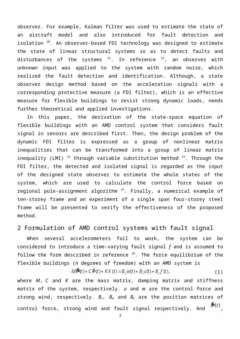
the deficiency when the whole states are too hard to be measured directly in a high-rise building. Since acceleration is easier to be measured than displacement and velocity, it can be used to construct the state observer that was more robust 17. Based on the state observer and a suitable control strategy, the control system can restrain the structural response timely 18, 19. Noticeably, due to such adverse circumstances as mechanical damage, environmental damage, and lack of maintenance, the attached accelerometers sometimes may malfunction or even fail. An observer-based system is considered to introduce a fault signal that will seriously reduce the control performance. Therefore, the reliability and robustness of this system should be studied. FDI technologies are often used to estimate the state of the control system through an observer. For example, Kalman filter was used to estimate the state of an aircraft model and also introduced for fault detection and isolation 20. An observer-based FDI technology was designed to estimate the state of linear structural systems so as to detect faults and disturbances of the systems 21. In reference 22, an observer with unknown input was applied to the system with random noise, which realized the fault detection and identification. Although, a state observer design method based on the acceleration signals with a corresponding protective measure (a FDI filter), which is an effective measure for flexible buildings to resist strong dynamic loads, needs further theoretical and applied investigations.

In this paper, the derivation of the state-space equation of flexible buildings with an AMD control system that considers fault signal in sensors are described first. Then, the design problem of the dynamic FDI filter is expressed as a group of nonlinear matrix inequalities that can be transformed into a group of linear matrix inequality (LMI) 23 through variable substitution method 24. Through the FDI filter, the detected and isolated signal is regarded as the input of the designed state observer to estimate the whole states of the system, which are used to calculate the control force based on regional pole-assignment algorithm 25. Finally, a numerical example of ten-storey frame and an experiment of a single span four-storey steel frame will be presented to verify the effectiveness of the proposed method.

2 Formulation of AMD control systems with fault signalWhen several accelerometers fail to work, the system can be considered to introduce a time-varying

fault signal f and is assumed to follow the form described in reference 26. The force equilibrium of the flexible buildings (n degrees of freedom) with an AMD system is

(1)

where M, C and K are the mass matrix, damping matrix and stiffness matrix of the system, respectively. u and w are the control force and strong wind, respectively. Bs, Bw and Be are the position matrices of control

force, strong wind and fault signal respectively. And , and are the acceleration, velocity and displacement vector of the system, respectively.

The degrees of freedom of a whole control system (a building and its AMD system) become (n+1).

The state vectors of the system includes displacement and velocity. Therefore, its

dimension is 2 (n+1). Its derivative, which includes velocity and acceleration, is . Eq. (1) can be expressed into the state equation as

2

(2)

where A, B1 and B2 are the state matrix, the excitation matrix and the control matrix, respectively. E is the influence matrices of the fault signal on system state equation.

The observation equation can output displacement, velocity, and acceleration of the system. The displacement, velocity are used to verify the control effectiveness, and the acceleration to observe the whole system state.

(3)

where Y is the output vector, and C, D1 and D2 are the state output matrix, the direct transmission matrices of control force and external excitation, respectively. F is the influence matrices of the fault signal on system observation equation.

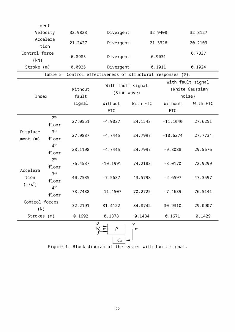
The system shown as Eq. (3) can be illustrated by Figure 1. P is the mathematical model of Eq. (3), and Co is the controller. When the fault signal exists in some certain sensors, an input signal f will be added into the system and will negatively impact the performance of the control system.

3 Dynamic FTC controller design

3.1 Dynamic FDI filter

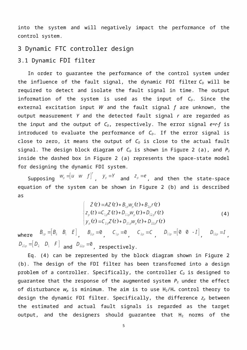
In order to guarantee the performance of the control system under the influence of the fault signal, the dynamic FDI filter CD will be required to detect and isolate the fault signal in time. The output information of the system is used as the input of CD. Since the external excitation input W and the fault signal f are unknown, the output measurement Y and the detected fault signal r are regarded as the input and the output of CD, respectively. The error signal e=r-f is introduced to evaluate the performance of CD. If the error signal is close to zero, it means the output of CD is close to the actual fault signal. The design block diagram of CD is shown in Figure 2 (a), and P2 inside the dashed box in Figure 2 (a) represents the space-state model for designing the dynamic FDI system.

Supposing , and , and then the state-space equation of the system can be shown in Figure 2 (b) and is described as

3

(4)

where , , , , , ,

and , respectively.Eq. (4) can be represented by the block diagram shown in Figure 2 (b). The design of the FDI filter

has been transformed into a design problem of a controller. Specifically, the controller CD is designed to guarantee that the response of the augmented system P2 under the effect of disturbance wp is minimum. The aim is to use H2/H∞ control theory to design the dynamic FDI filter. Specifically, the difference zp

between the estimated and actual fault signals is regarded as the target output, and the designers should guarantee that H2 norms of the transfer function between the interference input wp and the target output zp

is minimum. The input of CD is yp=Y, the output is the detected fault signal r, and the state-space equation of CD is

(5)

where Zf is the state vectors of CD.

To eliminate r and yp in Eq. (5), supposing , and then Eqs. (4) and (5) can be combined into a new closed-loop system as

(6)

where

(7)

The control system shown as Eq. (4) has a H∞ FDI filter 27, if and only if there exists a symmetric positive-definite matrix P such that the following inequality holds.

(8)

where ACL, BCL, CCL and DCL are determined by Eq. (7) and is a given positive constant. However, because inequality (8) is a nonlinear matrix inequality of the variables P, Af, Bf, Cf and Df, it is difficult to obtain the feasible matrix variables from the inequality directly. Therefore, the variable substitution method 24 needs to be used to transform the nonlinear matrix inequality (8) into a linear matrix inequality, and then the LMI toolbox can be used to solve the problem.

P and its inverse matrix P-1 are written as the block matrixes

(9)

4

where and . Supposing , then

(10)

Supposing

(11)

Supposing . Then

(12)

Supposing

(13)

Both sides of the matrix inequality (8) are pre and post multiplying and , respectively. Then the matrix inequality (8) is

(14)

The sub elements “*” of the upper matrix inequality can be obtained according to the symmetry of

the matrix. The matrix inequality (14) is pre and post multiplying , then

(15)

Supposing

(16)

Then, the inequality (15) is

(17)

The matrix P is a positive-definite matrix, if and only if the following inequality is established.

(18)

Then

5

(19)

where R, X, M, N, L and Df are the feasible solutions of the matrix inequalities (17) and (19).

Similarly, is a given positive constant. If and only if there exists symmetric positive-definite matrices P and Q such that the following inequalities hold.

(20)

(21)

(22)

The control system shown as Eq. (4) has a H2 FDI filter 24. The inequality (20) can be satisfied by the

inequality (8). The matrix inequality (21) is pre and post multiplying , then

(23)

The matrix inequality (23) is pre and post multiplying and , respectively. According to Eq. (12), the matrix inequality (23) is equivalent to

(24)

The matrix inequality (24) is pre and post multiplying , then

(25)

Using the variable substitution method 24, variables are defined as Eqs. (13) and (16), and then the matrix inequality (25) is equivalent to

(26)

where R, X, H, N and Df are the feasible solutions of the matrix inequalities (26) and (22).

Therefore, and are given positive constants for the control system shown as Eq. (6) that has a

dynamic FDI filter, if and only if the optimization problem is established.

(27)

s.t. 1) Inequality (17); 2) Inequality (19); 3) Inequality (26); 4) Inequality (22);

where R, X, M, Q, N, L and Df are the feasible solutions of the matrix inequalities (27). According to Eqs. (13) and (16), we get

6

(28)

The transfer function of the dynamic FDI filter is

(29)

According to Eq. (10), Eq. (29) is equivalent to

(30)

Then

(31)

and Df are the coefficient matrices of the dynamic FDI filter CD shown as Eq. (5) for the control system shown as Eq. (4).

3.2 Dynamic FTC controller with a state observer and a FDI filter

The nonlinear matrix inequalities are transformed into the form of the linear matrix inequalities based on the variable substitution method, and the solver “feasp” of LMI toolbox in MATLAB is used for solving the sub-optimal problem. The variables replaced by the method are restored, and then four coefficient matrices (Af, Bf, Cf and Df) of the dynamic FDI filter CD are solved. The fault signal in sensors from measuring signal Y is detected and isolated by the FDI filter CD. Based on these, a dynamic FTC controller can be built to control the structural responses. The control forces of the state feedback control system after fault isolation can be calculated by region pole-assignment algorithm.

The control forces of the FTC controller are described as

(32)

where G is a closed-loop feedback gain matrix based on regional pole-assignment algorithm 25. By substituting Eq. (32) into Eq. (2), we get

(33)

The state vector of each floor can be estimated effectively by using the state observer. Supposing

, , and , and a brief form of Eq. (33) is

(34)

The second equation of Eq. (34) can be written in the form of a partitioned matrix.

(35)

where Y1 is a vector of displacement and velocity of the structure and its AMD. Y2 is a vector of 7

acceleration, which is processed by the FDI filter, and , is the acceleration response with fault signal.

According to Eq. (35), the external excitation vector can be written as

(36)

By substituting Eq. (36) into Eqs. (34) and (35), we get

(37)

Supposing , , and , and Eq. (37) can be

written as

(38)

The state observer is described as

(39)

By substituting the second equation of Eq. (39) into the first equation, Y2 and Z can be used to

estimate the system state vectors .

(40)

where Go is the feedback gain of the observer. , which is an estimated vector of the system state of the structure and its AMD, is used to calculate the control force.

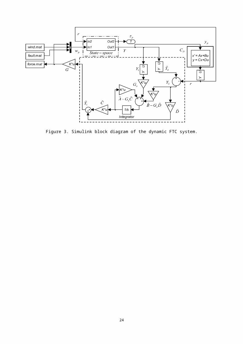
Based on the derivation above, the process of the FTC control system can be illustrated in Figure 3. The state-space equation (4) is shown by the point-line box, the state observer based on acceleration responses is depicted by the dashed box, and the symbol inside the black solid box represents the dynamic FDI filter CD.

3.3 Numerical verification

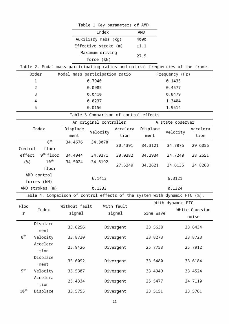
In this paper, a ten-storey frame has been constructed for numerical analysis. The height and total mass of this structure are 33 m and 892.9 tons, respectively. The lumped mass method is used to build the mass matrix for the structure. A unit force is applied to each particle floor of the structure, and then the displacement at each floor is obtained and combined into the flexibility matrix. The stiffness matrix can be easily obtained, as the inverse of the flexibility matrix. The AMD control device is assumed to be installed on the eighth floor and is only used to control the horizontal vibration along the minor axis. Key parameters of AMD are listed in Table 1. Structural frequencies and modal mass participating ratios 28 of the ten-storey frame, which are calculated using the model constructed in Matlab, are listed in Table 2.

Based on Davenport spectrum, a ten-year return period fluctuating wind speed is generated for

numerical analysis. Mixed autoregressive-moving average (MARMA) model 29 is proposed to simulate

8

the stochastic process. The fluctuating wind load on each floor can be calculated by Eq. (41).

(41)

where Pi is the fluctuating wind load at ith floor, and is the air density. is the average wind speed

at ith floor. is the fluctuating wind speed that is associated with height and time. and S are the shape factor of a building and the area of windward side, respectively.

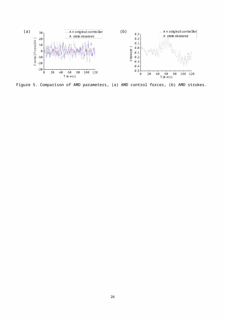
Under the above ten-year return period wind load, an original controller and a state observer both based on regional pole-assignment algorithm are designed for the ten-storey frame. The structural responses of the eighth floor under uncontrolled and controlled are shown in Figure 4, and AMD parameters of different systems are shown in Figure 5. Table 3 presents the maximum responses, control effects and values of AMD parameters. In this paper, the control effect is quantified as the ratio between dynamic responses of the structure with and without control, and AMD parameters include control force and stroke.

Figures 4, 5 and Table 3 show that the original controller and the state observer both based on pole-assignment algorithm can obviously reduce the wind vibration response. Specifically, the maximum variations of the displacement, velocity and acceleration control effects between two different systems are only 0.24%, 0.21% and 2.70%, and the AMD parameters of the state observer increases by 0.1708N and -0.0009m. Therefore, the acceleration response obtained from the optimal placement scheme of sensors can be rationally used as a feedback signal for the state observer that also can guarantee that the system has the same superior control effect and stable AMD parameters as the original controller.

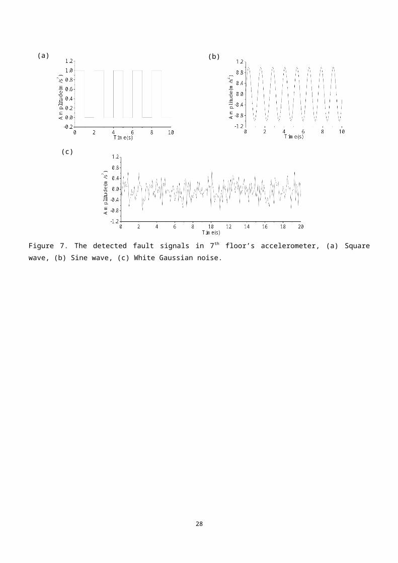
A dynamic FTC controller with a state observer and a FDI filter is then designed for the ten-storey frame. The accelerometer in the seventh floor is assumed to fail to work, and three forms of artificially added fault signals are assumed, i.e. square wave (the amplitude of 1m/s2, the period of 2s and the width of 1s), sine wave (the amplitude of 1m/s2, the period of 2s) and white Gaussian noise (the power is 0.1dBW, the load impedance is 0.1 ), as shown in Figure 6. The dimension of the fault signal f(t) of the ten-storey frame is 11 1. The signals shown in Figure 6 are added in seventh floor’s accelerometer. Time history analysis can be achieved by simulink toolbox in Matlab, and the duration of the whole process is 600s.

Under these scenarios, the effectiveness of the dynamic FDI filter will be verified by comparing the detected fault signal with the artificially added one. The detected fault signals in seventh floor’s accelerometer are shown in Figure 7, and the errors of added and detected fault signals in seventh floor’s accelerometer are shown in Figure 8. Based on the results, under both conditions, the detected trend and amplitude of signals from the fault accelerometer are equal to the assumption. Moreover, Figure 8 shows that the amplitudes of the errors are almost zero. Therefore, the FDI filter CD designed in this paper can used to detect the location and the amplitude of the fault signal correctly.

The performance of the designed FTC controller is then verified by comparing with the system without fault signal (No fault signal). Under a ten-year return period wind load, the structural responses and the AMD parameters of different control systems with and without fault signal are shown in Figures 9 and 10. Fault signals with dynamic FTC stands for control systems with different time-varying fault signals (square wave, white Gaussian noise) and a dynamic FTC controller. In the figures, dashed lines

9

represent the response of the structure without control under the wind load, and the solid lines show the response of the structure with control. The corresponding control effects (defined as the ratio between controlled and uncontrolled responses) and AMD parameters are listed in Table 4.

From Figures 9, 10 and Table 4, (1) When the sensor has no fault signal, the controller based on regional pole-assignment algorithm can effectively reduce the structural response. When the sensor fails, the control system that does not take the isolation measure is to diverge. Therefore, the fault signal in sensor cannot be ignored. The design of the dynamic FDI filter can isolate the fault signal, which is very important for the control system. (2) When the sensor has a sine wave fault signal, the dynamic FTC controller can effectively restrain the structural response, and its control effects are nearly equivalent to the system without a fault signal. Specifically, the maximum variations of the displacement, velocity and acceleration control effects between two different systems are only 0.06%, 0.05% and 0.17%. Therefore, the developed dynamic FTC controller can effectively detect and isolate the fault signal. Also, the dynamic FTC controller can maintain the stability of AMD parameters, which are consistent with the system without fault signal. Specifically, AMD parameters of the FTC controller increase only by 0.0046N and 0.0086m. The same result can be obtained when the fault signal is white Gaussian noise.

4 Experimental verificationFigure 11 shows an experimental system 16 of a four-storey steel frame with an AMD control device

installed on the fourth floor. The acceleration signals of the second and fourth floors were used as the feedback signal for a controller to calculate the real-time control forces. A servo motor can acquire the forces from an EtherCAT bus system and was used to add these forces to control the structure. The structural response signals of the second, third, fourth floors were used to verify the control effectiveness.

To verify the efficiency of the developed method, the FTC controller is applied to the experimental system. The original signal is monitored by the second, fourth floor acceleration response of the controlled structure. Then the observer is used to get estimated states to calculate the control forces. The loading frequency of the system is 1Hz, that is, the peak value of the corresponding excitation force is 45.89N, and the wave form of this force is sinusoidal. Under the above excitation load, the estimated and measured values of the structural responses are showed in Figure 12. The duration of each scenario is 300s, and Figure 12 only gives data in 30s.

From Figure 12, (1) The design method of the state observer based on the accelerations of partial floors is proposed in this paper, which can estimate the whole state vectors of the system accurately. (2) In the estimation results, the estimated displacement of the fourth floor is 0.0385 m, and in the actual results, the measured displacement is 0.0385 m, the displacement observation error is 0.4 10-3m. The estimated velocity is 0.1479 m/s, the measured velocity is 0.1429 m/s, the velocity observation error is 0.5 10-2m/s. Both above two observation errors are really minor. (3) There are two main reasons causing the observation errors of the displacement and velocity, a) When the floor is moved to the place that has maximum horizontal displacement, the model has a slight and rapid vibration due to the coupling effect of vertical and horizontal sinusoidal loads. b) There is a noise signal around the experimental system. It will affect if sensors can accurately measure the feedback signal or not.

When the accelerometer at the second floor fails to work, three forms of artificially added fault signals are assumed as shown in Figure 6. The detected fault accelerometer signal at second floor is

10

shown in Figure 13. The detected fault accelerometer signals (square and sine wave) at the second floor changes with time, and the amplitudes (1.055989 m/s2 and 1.055783 m/s2) of the detected fault signals is close to the artificially added fault signal (1 m/s2). For white Gaussian noise, the detected one is pretty close to the origin one. Therefore, the FDI filter designed in this paper can used to detect the location and the amplitude of the fault signal correctly.

Choosing two types of fault signals (sine wave and white Gaussian noise) as an example, the structural responses of different control systems with and without FTC are shown in Figure 14, and the corresponding control effects and AMD parameters are listed in Table 5.

Based on the results, (1) AMD control system will increase the structural response and play a negative role when the sensor fails, if designers do not take any isolation measures. Specifically, the displacement and acceleration control effects of the system with fault signal are all negative numbers. Therefore, it is important to design a FTC controller with a state observer and a FDI filter to detect and isolate the fault signal. (2) For sine wave fault signal, control effects and AMD parameters of the FTC system are close to the system without fault signal. Specifically, the maximum variations of the displacement, velocity and acceleration control effects between two different systems are 3.32% and 3.47%, and the AMD parameters of the FTC controller increase by 2.66N and -0.0208m. For white Gaussian noise, the maximum variations of the different control effects between two different systems are 1.44% and 6.60%, and the AMD parameters decrease by 3.13N and 0.0263m. Therefore, the FTC controller can detect and isolate the fault signal effectively, and it can also restrain the structural responses and maintain the AMD parameters in the appropriate range. (3) The structural response does not completely obey the sine law due to the interaction between the AMD system and the structure, and the coupling of the horizontal and the vertical structural vibrations. (4) AMD device is placed in the fourth floor of the structure. Further, the acceleration control needs high frequency control force that will mitigate the structural high-order modes. Therefore, the control effect of third floor, which has an opposite high-order phase with the fourth floor, will be significantly less than the control effect of second, fourth floors.

5 ConclusionsIn this paper, a state observer is designed for the considered problem which is that state vectors of

the control system are difficult to directly measure. Moreover, fault signal has a negative influence on the designed state observer. To address this issue, a dynamic FDI filter design method is presented to achieve the detection and isolation of the fault signal. Finally, a dynamic FTC controller design method that combines a state observer and a FDI filter can be finished. A numerical example and an experiment are presented to verify the effectiveness of the proposed method. Based on the results, the following conclusions can be drawn.

(1) A well-designed dynamic FDI filter can be used to detect the location and the amplitude of the fault signal correctly.

(2) The state observer based on the accelerations of each floors can accurately observe the whole states of the system, and it has superior control effect and stable AMD parameters.

(3) When the sensor fails to work, the system will be regarded as introducing a new input signal that will bring negative interference to the system. AMD control system without consideration of this issue

11

will increase the structural response when the fault signal in sensor presents. (4) The FTC controller is combined with a state observer and a dynamic FDI filter. It can tolerate the

fault signal in accelerometers, effectively control the structural response and maintain the stability of AMD parameters. Its control effects and AMD parameters are close to the system without fault signal. Therefore, it can enhance the robustness of the control system.

Even with fault signals, the control performances are still stable, as demonstrated by above results. Therefore, the dynamic FTC controller described in the paper can be regarded as robust control. The dynamic FDI filter designed in this paper can be applied widely, but it may have difficulties to achieve the process of fault-tolerance control in engineering practices through hardware devices. Thus, future efforts in this direction can be focused on a static FDI filter shown as a gain matrix to achieve the conversion between the measuring output with fault signal and the real output.

Acknowledgments: The research described in this paper was financially supported by the Major International (Sino-US) Joint Research Project of the National Natural Science Foundation of China (Grant No. 51261120374), the National Natural Science Foundation of China (Grant No. 51378007), Shenzhen Technology Innovation Program-Technology Development Projects (Grant No. CXZZ20140904154839135), and special funds of independent innovation industry development of Shenzhen Nanshan District (Grant No. KC2015ZDYF0009A).

6 References1. Cao, H., Reinhorn, A. M., and Soong, T. T., Design of an active mass damper for a tall TV tower in

Nanjing, China. Eng Struct, 1998, 20, 134-143. 2. Yamamoto, M., Aizawa, S., Higashino, M., and Toyama, K., Practical applications of active mass

dampers with hydraulic actuator. Earthq Eng Struct D, 2001, 30, 1697-1717. 3. Ricciardelli, F., Pizzimenti, A. D., and Mattei, M., Passive and active mass damper control of the

response of tall buildings to wind gustiness. Eng Struct, 2003, 25, 1199-1209. 4. Ikeda, Y., Sasaki, K., Sakamoto, M., and Kobori, T., Active mass driver system as the first application

of active structural control. Earthq Eng Struct D, 2001, 30, 1575-1595. 5. Basu, B., Bursi, O. S., Casciati, F., Casciati, S., Del Grosso, A. E., Domaneschi, M., Faravelli, L.,

Holnicki-Szulc, J., Irschik, H., and Krommer, M., et al., A European Association for the Control of Structures joint perspective. Recent studies in civil structural control across Europe. Struct Control Hlth, 2014, 21, 1414-1436.

6. Chen, J., and Patton, R. J., Robust model-based fault diagnosis for dynamics systems. Boston: Kluwer Academic Publishers, 1999.

7. Zhang, Y. M., and Jiang, J., Integrated active fault-tolerant control using IMM approach. IEEE T Aero Elec Sys, 2001, 37, 1221-1235.

8. Polycarpou, M. M., Fault acommodation of a class of multivariable nonlinear dynamical systems. IEEE Transaction on Automatic Control, 2001, 5, 736-742.

9. Marx, B., Koenig, D., and Georges, D., Robust fault-tolerant control for descriptor systems. IEEE T Automat Contr, 2004, 49, 1869-1875.

10. Mehra, R. K., and Peschon, J., Innovations approach to fault detection and diagnosis in dynamic systems. Automatica, 1971, 7, 637.

12

11. Shao, S., Watson, A. J., Clare, J. C., and Wheeler, P. W., Robustness Analysis and Experimental Validation of a Fault Detection and Isolation Method for the Modular Multilevel Converter. IEEE T Power Electr, 2016, 31, 3794-3805.

12. Rios, H., Davila, J., Fridman, L., and Edwards, C., Fault detection and isolation for nonlinear systems via high-order-sliding-mode multiple-observer. Int J Robust Nonlin, 2015, 25, 2871-2893.

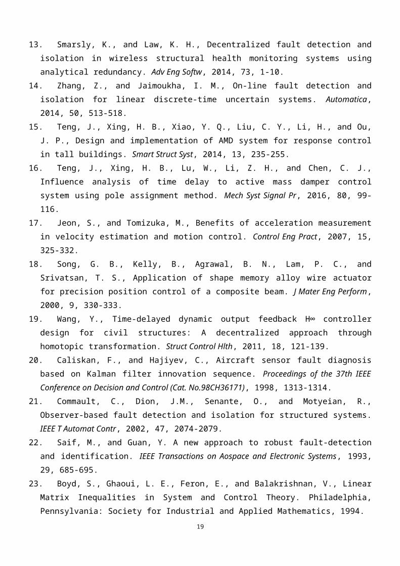
13. Smarsly, K., and Law, K. H., Decentralized fault detection and isolation in wireless structural health monitoring systems using analytical redundancy. Adv Eng Softw, 2014, 73, 1-10.

14. Zhang, Z., and Jaimoukha, I. M., On-line fault detection and isolation for linear discrete-time uncertain systems. Automatica, 2014, 50, 513-518.

15. Teng, J., Xing, H. B., Xiao, Y. Q., Liu, C. Y., Li, H., and Ou, J. P., Design and implementation of AMD system for response control in tall buildings. Smart Struct Syst, 2014, 13, 235-255.

16. Teng, J., Xing, H. B., Lu, W., Li, Z. H., and Chen, C. J., Influence analysis of time delay to active mass damper control system using pole assignment method. Mech Syst Signal Pr, 2016, 80, 99-116.

17. Jeon, S., and Tomizuka, M., Benefits of acceleration measurement in velocity estimation and motion control. Control Eng Pract, 2007, 15, 325-332.

18. Song, G. B., Kelly, B., Agrawal, B. N., Lam, P. C., and Srivatsan, T. S., Application of shape memory alloy wire actuator for precision position control of a composite beam. J Mater Eng Perform, 2000, 9, 330-333.

19. Wang, Y., Time-delayed dynamic output feedback H∞ controller design for civil structures: A decentralized approach through homotopic transformation. Struct Control Hlth, 2011, 18, 121-139.

20. Caliskan, F., and Hajiyev, C., Aircraft sensor fault diagnosis based on Kalman filter innovation sequence. Proceedings of the 37th IEEE Conference on Decision and Control (Cat. No.98CH36171), 1998, 1313-1314.

21. Commault, C., Dion, J.M., Senante, O., and Motyeian, R., Observer-based fault detection and isolation for structured systems. IEEE T Automat Contr, 2002, 47, 2074-2079.

22. Saif, M., and Guan, Y. A new approach to robust fault-detection and identification. IEEE Transactions on Aospace and Electronic Systems, 1993, 29, 685-695.

23. Boyd, S., Ghaoui, L. E., Feron, E., and Balakrishnan, V., Linear Matrix Inequalities in System and Control Theory. Philadelphia, Pennsylvania: Society for Industrial and Applied Mathematics, 1994.

24. Yu, L., Robust Control-Linear Matrix Inequalities Approach. Beijing: Tsinghua University Press, 2002.

25. Haddad, W. M., and Bernstein, D. S., Controller-design with regional pole constraints. IEEE T Automat Contr, 1992, 37, 54-69.

26. Gao, Z., and Ding, S. X., State and disturbance estimator for time-delay systems with application to fault estimation and signal compensation. IEEE T Signal Proces, 2007, 55, 5541-5551.

27. Gahinet, P., and Apkarian, P., A linear matrix inequality approach to h∞ control. Int J Robust Nonlin, 1994, 4, 421-448.

28. Clough, R.W., and Penzien, J., Dynamics of Structures. U.S.: McGraw-Hill Inc, 1975.29. Hannan, E.J., The identification of vector mixed autoregressive-moving average system. Biometrika,

1969, 56, 223-225.

13

14

Table 1 Key parameters of AMD.Index AMD

Auxiliary mass (kg) 4000Effective stroke (m) ±1.1

Maximum driving force (kN) 27.5

Table 2. Modal mass participating ratios and natural frequencies of the frame.Order Modal mass participation ratio Frequency (Hz)

1 0.7940 0.14352 0.0985 0.45773 0.0410 0.84794 0.0237 1.34045 0.0156 1.9514

Table.3 Comparison of control effects

IndexAn original controller A state observer

Displacement

Velocity AccelerationDisplacemen

tVelocity Acceleration

Control effect (%)

8th floor 34.4676 34.8078 30.4391 34.3121 34.7876 29.60569th floor 34.4944 34.9371 30.0382 34.2934 34.7240 28.2551

10th floor 34.5024 34.8192 27.5249 34.2621 34.6135 24.8263AMD control forces

(kN)6.1413 6.3121

AMD strokes (m) 0.1333 0.1324Table 4. Comparison of control effects of the system with dynamic FTC (%).

Floor Index Without fault signal With fault signalWith dynamic FTC

Sine waveWhite Gaussian

noise

8th

Displacement

33.6256 Divergent 33.5638 33.6434

Velocity 33.8730 Divergent 33.8273 33.8723Acceleration 25.9426 Divergent 25.7753 25.7912

9th

Displacement

33.6092 Divergent 33.5480 33.6184

Velocity 33.5387 Divergent 33.4949 33.4524Acceleration 25.4334 Divergent 25.5477 24.7110

10th

Displacement

33.5755 Divergent 33.5151 33.5761

Velocity 32.9823 Divergent 32.9408 32.8127Acceleration 21.2427 Divergent 21.3326 20.2103

Control force (kN) 6.8985 Divergent 6.9031 6.7337Stroke (m) 0.0925 Divergent 0.1011 0.1024

Table 5. Control effectiveness of structural responses (%).

IndexWithout fault

signal

With fault signal (Sine wave)

With fault signal (White Gaussian noise)

Without FTC With FTC Without FTC With FTCDisplacemen 2nd floor 27.0551 -4.9037 24.1543 -11.1040 27.6251

15

t (m)3rd floor 27.9837 -4.7445 24.7997 -10.6274 27.77344th floor 28.1198 -4.7445 24.7997 -9.8088 29.5676

Acceleration (m/s2)

2nd floor 76.4537 -10.1991 74.2183 -8.0170 72.92993rd floor 40.7535 -7.5637 43.5798 -2.6597 47.35974th floor 73.7438 -11.4507 70.2725 -7.4639 76.5141

Control forces (N) 32.2191 31.4122 34.8742 30.9310 29.0907Strokes (m) 0.1692 0.1878 0.1484 0.1671 0.1429

Pwf

u

Co

Y

Figure 1. Block diagram of the system with fault signal.

16

(a)

Pwf

u

CD

Y

r

e

P2

yp

(b)

P2wp

r

CD

zp

yp

Figure 2. Block diagram of the dynamic FDI system, (a) Block diagram 1, (b) Block diagram 2.

17

Figure 3. Simulink block diagram of the dynamic FTC system.

18

(a) (b)

(c) (d)

Figure 4. Comparison of structural responses to 8th floor under uncontrolled and controlled by an original controller, (a) Displacements, (c) Accelerations. And controlled by a state observer, (b) Displacements, (d) Accelerations.

19

(a) (b)

Figure 5. Comparison of AMD parameters, (a) AMD control forces, (b) AMD strokes.

20

(a) (b)

(c)

Figure 6. The artificially added fault signals in 7th floor’s accelerometer, (a) Square wave, (b) Sine wave, (c) White Gaussian noise.

21

(a) (b)

(c)

Figure 7. The detected fault signals in 7th floor’s accelerometer, (a) Square wave, (b) Sine wave, (c) White Gaussian noise.

22

(a) (b)

(c)

Figure 8. The errors zp between two types of fault signals in 7th floor’s accelerometer, (a) Square wave, (b) Sine wave, (c) White Gaussian noise.

23

(a) (b)

(c) (d)

(e) (f)

Figure 9. Comparison of structural responses to 8 th floor, (a), (b) Under uncontrolled and controlled without fault signal, (c), (d) Considering sine wave fault signal and controlled with dynamic FTC, (e), (f) Considering white Gaussian noise and controlled with dynamic FTC.

24

(a) (b)

Figure 10. Comparison of AMD parameters, (a) AMD control forces. (b) AMD strokes.

25

(a) (b)

A reducer

A servo motor

Accelerometer 3

Accelerometer 4

Accelerometer 2

Laser displacementsensor 2

Laser displacementsensor 3

Laser displacementsensor 1

An inverter

A dSPACE system

Computer

Controller

EK1100

EL3008 EL4034

AX5000

EtherCATbus system

m1

m2

m3

m4

Accelerometer 1

ma ka ca

k4 c4

k3 c3

k2 c2

k1 c1

Figure 11. Pictures of the steel frame structure, (a) Practicality, (b) Exhibition.

26

(a) (b)

Figure 12. Comparison between measured and estimated system state in 4th floor: (a) Displacements. (b) Velocities.

27

(a) (b)

(c)

Figure 13. The detected fault signal in 2th floor’s accelerometer of the experimental system, (a) Square wave, (b) Sine wave, (c) White Gaussian noise.

28

(a) (b)

(c) (d)

(e) (f)

Figure 14. Comparison of structural responses to 4th floor of the experimental system, (a), (b) Under uncontrolled and controlled without fault signal, (c), (d) Considering sine wave fault signal and controlled with dynamic FTC, (e), (f) Considering white Gaussian noise and controlled with dynamic FTC.

29