introduction - university of oxfordpeople.maths.ox.ac.uk/beentjes/essays/computational... · range...

COMPUTATIONAL ELECTROCHEMISTRY

CASPER H. L. BEENTJES

Mathematical Institute, University of Oxford, Oxford, UK

Abstract. We derive a mathematical model for the dynamics of redox reactions at an electrode-

liquid interface when an external potential is applied to the electrode. The model couples

chemical transport with electron kinetics and the set-up of the model allows for a generalrange of external potentials. We further investigate the resulting dynamics of five types of

external potential. Numerical simulations are performed using a finite difference and a Cheby-shev collocation approach yielding perfect agreement with theory whenever available.

1. Introduction

Electrons form a key ingredient in many chemical reactions, particularly in the case of redoxreactions. This particular type of reaction encompasses a wide range of phenomena. Examplesare the corrosion of metals and many important biological reactions, such as the oxidation ofglucose, which is used to provide energy to cells.

Electrochemistry concerns the study of such chemical reactions in a typical set-up where thereis a redox reaction between a solid electrode and a solute, often dissolved in liquid. Electrontransfer can take place when electrons in a chemical have sufficient energy to move from theirorbits into lower energy orbits around different molecules. The potential of a chemical determinesthe energy of its electrons and therefore dictates the electron transfer. This makes the set-up ofelectrochemistry so beneficial, as it allows one to directly control the potential of the electrode byuse of an external power supply. Information about the electron transfer can in turn be accuratelyacquired by measurement of the current that flows due to the transfer. This way of exploring thedynamics is called amperometry. The specific case where one measures a changing current as aresult of an externally applied potential is also known as voltammetry. Many different techniquesof voltammetry have been proposed, which all differ in the way they apply the potential on theelectrode. For example, a steady potential or a time-dependent potential. Traditional methodssuch as spectroscopy often fail to capture the electron dynamics because of the size and velocityof the electrons involved. Voltammetry, on the other hand, can yield direct insight into thekinetics of the electron transfer by measurement of the current, which makes it an indispensabletool in analytical chemistry.

This paper studies the mathematical modelling of electrochemical problems. We examinemodels for five widespread voltammetry types, chronoamperometry, linear sweep voltammetry,cyclic voltammetry, alternating current voltammetry and square wave voltammetry. Firstlywe introduce the basics of mathematical modelling of the electrode processes in combinationwith transport of the chemicals by means of differential equations. Subsequently we analyse the

E-mail address: [email protected]: Hilary term 2015.

2010 Mathematics Subject Classification. 78A57, 65M70.This text is based on a technical report for the Scientific Computing Case Study during Hilary 2015 for the

Oxford Mathematics MSc. in Mathematical Modelling & Scientific Computing.

1

mailto:[email protected]

2 C. H. L. BEENTJES

resulting mathematical models and in some special cases analytical solutions can be found. Thereis, however, a wider class of voltammetry problems for which exact solutions are as yet unknownand to investigate these, we utilise numerical simulations to find approximate solutions.

2. Mathematical model

We will focus on the problem of a planar electrode as depicted in Figure 1. The assumption ismade that the size of the electrode is such that we can neglect the effect of the edges and thereforeconsider a one-dimensional problem with only the vertical space-coordinate x. We consider twochemical species A and B which can form and react at the surface of the electrode. The modelaims to describe the concentrations of the chemicals, cA(x, t) and cB(x, t) respectively.

x

working electrode

solvent + solutes A,B

e− e− e−

B A

V

Figure 1. Schematic diagram of a planar electrode problem. The workingelectrode is in contact with a liquid containing some solvent in which the solutesA,B are dissolved. At the electrode surface a reaction of B into A takes place.Note that the contra reaction also occurs if the reaction is reversible, but it isnot depicted here. A counter electrode needs to be present to close the electricalcircuit.

In experiments the observed results, such as the current, will often reflect only local effectsat the electrode. Therefore we assume that the counter electrode is far away from the workingelectrode, making its influence on the working electrode negligible.

The main processes responsible for change in concentration are the transport of chemicalsthrough the solvent and the reaction of the chemicals at the electrode, which need to be incor-porated in the model.

2.1. Transport of chemicals. The chemicals A and B can be transported through the liquidby three basic processes, namely diffusion, convection and migration. Here, migration is theeffect that charged species will be either repelled or attracted by the electrode surface as weapply a potential. Consequently, the change of concentration would be described by a Nernst-Planck equation, which describes mass conservation for a charged chemical species in a solventand incorporates all three transport types.

For reasons of simplicity we will, however, consider a more elementary problem where weneglect effects of migration and convection. This can be achieved experimentally as well. Toneglect the convection effects we can consider an unstirred solution over a short time so thatthere is no natural convection due to temperature or external convection of the chemicals. Themigration is often excluded from experiments by adding an auxiliary electrolyte to the liquid,which does not react or influence reactions at the electrode surface. This results in an effectivescreening of the potential gradient induced by the electrode and therefore makes the migrationof A and B negligible.

COMPUTATIONAL ELECTROCHEMISTRY 3

The Nernst-Planck equation now reduces to Fick’s second law describing the transport of masspurely due to diffusion

(1)

∂cA∂t

= DA∂2cA∂x2

,

∂cB∂t

= DB∂2cB∂x2

,

where DA,B is a diffusion coefficient and it can possibly be different for both species.This gives PDEs for cA and cB , which need to be supplemented by suitable initial condi-

tions and four boundary conditions to close the system. We assume that initially we have ahomogeneous solution of purely A with bulk concentration cbulk, i.e.

(2)

{cA(x, 0) = cbulk,

cB(x, 0) = 0.

Now assume that the vertical direction is sufficiently large, i.e. the volume of the chemical cellis large. Furthermore recall that in order to neglect convection we had to consider the problemon a small enough timescale. We then view the chemical cell as a semi-infinite domain, where atlarge distances from the electrode the concentrations are undisturbed by the electrode and thusremain at the bulk values. This gives the far-field boundary conditions

(3)

{cA(x, t) → cbulk

cB(x, t) → 0as x→∞, t > 0.

Two more boundary conditions are needed and they are prescribed at the electrode-liquid inter-face. The first one follows from the conservation of mass at the surface. If we use Fick’s firstlaw, giving the flux of a diffusing chemical, we find that

(4) DA∂cA∂x

+DB∂cB∂x

= 0 at x = 0, t > 0.

The last boundary condition will depend on the applied potential at the electrode resulting inredox reactions.

2.2. Electron transfer and current. We will consider a reductant-oxidant couple A,B react-ing in a redox reaction at the electrode surface

(5) Akoxkred

B + ne−,

where kred and kox are the reaction rates of both reactions. The total current I at the electrodedue to the redox reaction (5) is directly related to the flux of the chemicals at the surface byFaraday’s law of electrolysis

(6) I = nFADA∂cA∂x

∣∣∣∣x=0

,

where A is the surface area of the working electrode and F is the Faraday constant.Note that the current involves the flux of molecules A at the electrode-liquid interface. The

chemicals will react following (5) and often this reaction can be modelled as a first-order reaction.In that case the rate-law equation at the surface gives a reaction flux of A. If we combine thiswith Fick’s first law for the diffusion flux and demand that there is no net-flux of A through theelectrode we find the remaining boundary condition

(7) DA∂cA∂x

= koxcA − kredcB , at x = 0.

4 C. H. L. BEENTJES

There are however two remaining unknowns in equation (7), the reaction rates. A widely usedempirical model for the reaction rates is the Arrhenius equation

(8) k = K exp

(−∆G‡

RT

),

where R is the universal gas constant, T the temperature and ∆G‡ is the activation Gibbs freeenergy. As the potential of the electrode, denoted by E, controls the energy of the electronson the working electrode it is expected that this will influence the Gibbs free energy ∆G‡(E).Decreasing the potential of the electrode will move the electrons on the electrode to a higher

energy level. This stimulates the uptake of electrons by the oxidant A, thus lowering ∆G‡red and

increasing ∆G‡ox. An opposite effect is expected if we ramp up the potential. Empirical modelshave indeed been proposed for ∆G‡ and arguably the most simple relation, a linear relation, isgiven by the Butler-Volmer model [2, 5]

∆G‡red = ∆G‡0 + αnF (E − E0f ),(9a)

∆G‡ox = ∆G‡0 − (1− α)nF (E − E0f ),(9b)

where α ∈ [0, 1] is the charge transfer coefficient and E0f is the formal potential. At the formal

potential the rates of both equations are equal. The charge transfer coefficient reflects thesymmetry in the effect of the potential on the energy barrier. Often a value of α = 1/2 is taken,reflecting a symmetric effect of E on the barrier.

The boundary condition (7) together with the Butler-Volmer kinetics becomes now at x = 0

DA∂cA∂x

= K0

(cA exp

{(1− α)

nF (E − E0f )

RT

}− cB exp

{−α

nF (E − E0f )

RT

}),(10)

where K0 is the reaction rate constant at the formal potential. This reaction rate is a measurefor the reversibility of the reaction at the reaction surface. For high K0 the redox reactions willbe fast and the chemicals will establish an equilibrium at the electrode surface, the reaction issaid to be reversible. For low K0, on the other hand, the electron transfer rate is slow and thechemicals cannot sustain an equilibrium, these reactions are known as quasi-reversible reactions.

This completes the model for the chemical dynamics; two governing PDEs (1) with initialconditions (2) and boundary conditions (3,4,10).

2.3. Non-dimensionalisation. To keep analysis tractable we non-dimensionalise the model byusing the following dimensionless quantities

a =cAcbulk

, b =cBcbulk

, d =DB

DA, x =

x

L, t =

DAt

L2(11a)

I =L

nFADAcbulkI, θ =

nF

RT(E − E0

f ), k0 =L

DAK0.(11b)


This results in the following non-dimensional system of equations with initial and boundaryconditions which will be considered in this paper

(12a)

(12b)

(12c)

(12d)

(12e)

(12f)

(12g)

at = axx for x > 0, t > 0,

bt = dbxx for x > 0, t > 0,

a(x, 0) = 1, b(x, 0) = 0,

a(x, t)→ 1, b(x, t)→ 0 as x→∞, t > 0,

ax(0, t) + dbx(0, t) = 0 for t > 0,

ax(0, t) = k0

[a(0, t)e(1−α)θ − b(0, t)e−αθ

]for t > 0,

I(t) = ax(0, t).

3. Numerical methods

As mentioned earlier, analytical progress on the formulated system cannot always be expected,which is mainly due to the boundary conditions. Therefore we often use numerical methods toexplore the model dynamics. In this paper we use the method of lines [8]. We convert the PDEsto a system of ODEs by first discretising the PDEs in the spatial direction. This replaces thecontinuous a(x, t) by a vector a(t) = [a1(t), . . . , am(t)] defined on a discrete grid with m points{xj}mj=1, such that a(xj , t) ≈ aj(t). A similar transformation is applied to b(x, t). By discretisingin the spatial direction we must replace the continuous (linear) diffusion operators in (12a, 12b)with linear operators, i.e. matrices, on a(t) and b(t). We will denote this as a generic matrix D2,the second order differentiation matrix. The result is an ODE system, with the approximationof (12a)

(13)da(t)

dt= D2a(t).

The equation for b(t) is the same except for the factor d. The boundary conditions and initialconditions are applied pointwise. This ODE-system is then solved along lines of constant position,hence the method of lines, using a suitable ODE integration scheme.

3.1. Spatial discretisation. Two different approaches are followed for the spatial discretisation,reflecting a different choice of grid points {xj}mj=1. Note that the continuum spatial domain is[0,∞), but numerically this is not feasible as we need to work with a finite number of spatialpoints. Therefore we will truncate the domain for some sufficiently large x = x∗. We assumethat the electrode process does not influence the solution at x > x∗ and set a(x∗, t) = 1 andb(x∗, t) = 0, the bulk values.

3.1.1. Finite differences. An widespread approach is the method of finite differences, which makesuse of an equispaced grid with grid-spacing ∆x. To approximate the second space-derivative weemploy a Taylor approximation of a(xj , t) to find the central difference approximation

(14) axx(xj , t) ≈aj+1(t)− 2aj(t) + aj−1(t)

(∆x)2.

The error in this approximation is O((∆x)2). From this we find the diffusion matrix

(15) D2 =1

(∆x)2

−2 1

1 −2. . .

. . .. . . 11 −2

.

6 C. H. L. BEENTJES

Note that we still need to take care of the boundary conditions and that we are interested in thecurrent. The far-field boundary conditions are Dirichlet boundary conditions in the truncateddomain and can be pointwise imposed at the last gridpoint. The situation at the electrode is,however, more cumbersome as the boundary conditions are of Neumann and Robin type. Acentral difference approximation is not possible, as we are at the boundary of the grid. Wechoose to employ a forward difference formula of second-order, so that the error order matchesthat of the diffusion operator. This yields

(16) ax(0, t) ≈ −3a1(t) + 4a2(t)− a3(t)

2∆x,

and similar formulation for bx(0, t). One of the main advantages of this method, as we shallsee in time-stepping of the ODE, is that the differentiation matrix has a sparsity pattern. Thepattern will be modified at the first and last row due to the boundary conditions, but the matrixremains sparse. A possible downside is the convergence of the method, which is predicted tobe of geometric order in space, second order to be more precise. The number of gridpointsN = O((∆x)−1) and convergence is thus O(N−2). Resultantly N needs to increase by a fairamount to gain more accuracy.

3.1.2. Chebyshev collocation. If the function we are approximating is smooth we can constructa method which has better convergence properties, a spectral method [10]. The convergence isof the order O(N−m) for any m > 0. This spectral convergence is significantly better than theconvergence for finite difference which has a fixed m > 0. Therefore this method can use farfewer points to obtain higher accuracy.

The main idea is that we expand our solution on a set of carefully chosen basis functions. Aswe have non-periodic boundary conditions we can use Chebyshev polynomials as basis functionsfor the spectral method. The spatial grid is a corresponding non-uniform Chebyshev grid. Thegain in convergence comes from the fact that we use global approximation of the function insteadof the local approximation as before. This global approximation of the function over the grid atevery point has the side-effect that the differentiation matrix will be a full matrix D2. To find thecurrent and first-derivatives at the electrode surface we use a global Chebyshev approximationof the derivative, just as we approximated the second derivative globally. We trade sparsity fora much lower number of grid-points compared to finite differences.

A positive side-effect of the use of Chebyshev collocation is the grid density near the electrodesurface. As the Chebyshev grid is non-uniform, with a higher density towards the boundary of thedomains, we have more resolution close to the electrode. We expect that most of the dynamicswill happen at the electrode. Therefore a more dense grid near the part of the domain werewe expect to see changes is likely to outperform a uniform grid. One could, of course, also findother ways to refine the grid close to the boundary. For example by using a previously discussedfinite difference approach in combination with an expanding mesh, c.f. Gavaghan & Bond [6].These methods, however, do not obtain spectral convergence as they are still based upon finitedifferences.

3.2. Time-stepping. A first note must be made on the coupling between a and b through theboundary conditions at the electrode (12e,12f). Consequently we need to solve for a and b simul-taneously. In order to approximate a solution to the ODE system governing the concentrationswe discretise the solution in time. We look for approximations ai at {ti}ni=0, with t0 = 0 andtn = Tmax such that a(xj , ti) ≈ aij . We assume the temporal points are equispaced with spacing∆t and thus tj = j∆t. Different methods can be used to discretise the time-derivative resultingin an (algebraic) system of the form

(17) ai+1 = F(ai).


Care must be taken as to what kind of integration scheme is used as the diffusion matrix D2 isill-conditioned for both spatial discretisations. In fact κ(D2) = O(Nm), with m = 2 for finitedifferences and m = 4 for the spectral method. In order for the time integration to be stablewe therefore use an implicit method in order to prevent severe constraints on the stepsize ∆tdue to the ill-conditioning of D2. In this paper we use the first order implicit Euler method toapproximate the time derivative at ti+1 by

(18)da(ti+1)

dt≈ ai+1 − ai

∆t,

with first order error O((∆t)−1).If we define C = [a,b]T , we can formulate our numerical discretisation of our model as

(19)

(I −∆t

(1 00 d

)⊗D2

)Ci+1 = Ci

for all points at the interior of the domain. We have to impose the boundary conditions atthe same time. This is achieved by imposing (19) on the interior domain points and using theremaining degrees of freedom at the boundary points in the algebraic system of equations toexplicitly impose the boundary conditions. In practice this is done by replacing the equationsgoverning the diffusion at the endpoints by explicit discretisations of the boundary conditions.This yields a closed 2m-system of equations, which by solving for Ci+1 lets us march through time.The theoretical convergence rates are observed to hold in practical simulations (see appendixA.1).

4. Voltammetry

We consider different types of voltammetry, all reflecting a specific way to specify the potentialas a function of time, i.e. θ(t) in the dimensionless model.

4.1. Chronoamperometry. We consider a reversible reaction at the electron surface, i.e. k0 �1, such that (12e) becomes

(20)a(0, t)

b(0, t)= e−θ,

which is the Nernst-equation in non-dimensional form, describing a perfectly reversible redoxreaction in absence of diffusion flux. We now assume that initially θ is such that no electrontransfer takes place and then ramp up the voltage instantaneously at t = 0, θ(t) = ΘH(t), whereH is the Heaviside step function and Θ the step-height of the potential.

4.1.1. Analytical solution. This problem now admits an exact solution which can be found bylooking for a similarity solution in the variable η = x/

√t. If we solve on x ∈ [0,∞) we find that

a(x, t) =

√deθ√

deθ + 1· erf

(x/2√t)

+1√

deθ + 1,(21a)

b(x, t) =eθ√

deθ + 1

(1− erf

(x/2√t))

.(21b)

Upon a differentiation with respect to x this yields the current

(22) I(t) =

√deθ√

deθ + 1· 1√

πt.

It is more insightful to consider the case of Θ� 1 so that we derive the more classical chronoam-perometry problem where at the electrode surface a(0, t) = 0, i.e. the potential is such that all

8 C. H. L. BEENTJES

A gets converted to B. Doing so we arrive at the Cotrell-equations for the chronoamperometryproblem

a(x, t) = erf(x/2√t),(23a)

b(x, t) =1√d

(1− erf(x/2

√dt)),(23b)

I(t) =1√πt.(23c)

Note that there is an inconsistency between the initial data provided by (12c) and the boundarycondition given by the Nernst-equation (20). Furthermore the current starts at zero at t = 0 andhas a discontinuity as we instantaneously increase the potential.

4.1.2. Numerical solution. Numerically we need to consider a finite domain and thus x∗ < ∞.In view of tractability we only treat the case of complete conversion of A so that we can use theCotrell-equations as a reference. We have three Dirichlet boundary conditions and one Neumannboundary condition which are implemented as mentioned in (3.2).

We can now observe that the error in a that is made by truncating the domain for the exactsolution is expected to be of order 1− erf(x∗/2

√t) (based on the difference at x∗), with a similar

expression available for b. We therefore choose x∗ such that the error by truncating the domainis smaller than the error made by the numerical scheme, as in that case the truncation is notnumerically noticeable.

0 0.5 1 1.5 2 2.5 3 3.5 4 4.5 50

1

2

3

4

5

6

7

8

9

t

I(t

)

NumericalExact

0 0.05 0.1 0.15 0.20

2

4

6

8

(a) Chronoamperometry current as a function oftime. Numerical solution is plotted after every50 timesteps.

0 5 10 15 20 25 300

0.2

0.4

0.6

0.8

1

x

Con

cent

rati

ona,b

Exact a(x, t)Numerical a(x, t)Exact b(x, t)Numerical b(x, t)

(b) Concentration profiles of a and b at t = 5with d = 4.

Figure 2. Plot of the current and the concentrations for a chronoamperometryproblem with d = 4. For the spatial discretisation a Chebyshev collocation withN = 20 is used and the timestep is ∆t = 10−4. The inset for the current showsa close-up of the results for small t.

Results of a numerical simulation with Chebyshev collocation are shown in Figure 2. Weobserve a very good agreement in concentration between the exact solution and the numerics.The numerical current appears to coincide with the Cotrell-equations as well. Note, however,that in Figure 2a the inset shows fair deviations from the exact solution for small t. This isdue to the inconsistency between the initial data and the boundary data and the singularity inI(t). This results in a boundary layer-like solution close to the electrode for small t. In orderto increasingly distinguish this effect we need to have an increasing number of points close to


the boundary. The effects of this initial inconsistency seem to disappear as t increases, which iscomforting, as in experiments one is often interested in the longer term behaviour of the current.

4.2. Linear sweep voltammetry. We return to a general k0 and consider now a linear increasein potential, called a linear sweep voltammetry (LSV). We choose a starting potential θ0 suchthat we have very few electron transfers occurring. Therefore we need kox � 1 at t = 0 as westart out with purely A and thus θ0 < 0. This yields

(24) θ(t) = θ0 + t.

Some authors prefer to introduce a scan rate ν for the potential, i.e. θ(t) = θ0 + νt, c.f. [3].This is, however, in some sense redundant. We can use a remaining degree of freedom in thenon-dimensionalisation of space as the problem doesn’t prescribe L in any natural way. If wetherefore introduce the new length scale l =

√νL and use this to non-dimensionalise, the factor

ν will drop out of the equations and we recover (24). Note that this yields the same dependenceof the current on the scan rate, I ∝

√ν, as used in the Randles-Sevcık equation [3]. This relation

is used experimentally to determine the reaction and diffusion constants by variation of the scanrate.

4.2.1. Semi-analytics for the current. Analytical expressions for the solution cannot be easilyderived in closed form for the general LSV problem. Nonetheless, if we again consider a reversiblereaction, k0 � 1, some progress can be made. In this case we observed that (12e) reduces tothe Nernst-equation (20). We can then derive an implicit relation for the current I(t) using aLaplace transform in time (see appendix A.3)

(25) F (t) =

√dπ√

d+ e−θ(t)=

∫ t

0

I(τ)√t− τ

dτ.

Note that this expression does not depend on the specific form of θ(t) and is thus valid forgeneral voltammetry types. One can note that the integrand diverges at τ = t, the edge of theintegration domain. This, however, does not necessarily mean that the integral diverges, for

example∫ 1

0log(x) dx = −1.

4.2.2. Numerical solution. The numerical solution of the concentrations is in essence the same asfor the chronoamperometry problem, only replacing a Dirichlet boundary condition by a Robinboundary condition.

A difference with chronoamperometry, however, is that we cannot provide an analytical so-lution for the concentrations to the problem due to a time-dependent potential. On the otherhand we still have an explicit expression for the current in case of k0 � 1, which we can useto compare with the numerical results. To effectively use this implicit integral equation for thecurrent, we approximate the integral numerically to find I(t). As noted before the integranddiverges at t = τ and this proves to be numerically difficult. Therefore we first reformulate theintegral equation by either partial integration or by an extra integration (see appendix A.3.1)

F (t) = 2

∫ t

0

I ′(τ)√t− τ dτ,(26a)

G(t) =

∫ t

0

F (s) ds = 2

∫ t

0

I(τ)√t− τ dτ.(26b)

The crux of the approximation of the current lies in the following observation

(27) F (n∆t) = 2

∫ n∆t

0

I ′(τ)√n∆t− τ dτ = 2

n−1∑i=0

∫ (i+1)∆t

i∆t

I ′(τ)√n∆t− τ dτ.

10 C. H. L. BEENTJES

A similar observation can be made for G(t) in (26b). By using the notation Ii = I(ti) we thenapproximate the integrals over (ti, ti+1), which for a certain class of approximations (see appendixA.3.1 for more details) yields a general form

(28)

∫ ti+1

ti

I ′(τ)√n∆t− τ dτ ≈ pi (Ii+1 − Ii)

√∆t,

where the constants pi depend on the particular form of approximation used. This can be usedto find an approximation to I(tn)

(29) In ≈1

pn−1

(F (n∆t)

2√

∆t+ p0I0 −

n−1∑i=1

(pi−1 − pi)Ii

).

The measured currents in voltammetry are often displayed in a voltammogram, a plot of thecurrent versus the applied potential. Since the potential in this case is simply a shifted versionof time this is equivalent to an I-t plot.

−10 −5 0 5 10 15 200

0.1

0.2

0.3

0.4

0.5

θ

I

k0 � 1k0 = 35k0 = 1k0 = 0.1

(a) LSV voltammogram for various k0.

−10 −5 0 5 10 15 200

0.1

0.2

0.3

0.4

0.5

θ

I

k0 � 1α = 0.3α = 0.5α = 0.7

(b) LSV voltammogram for various α.

Figure 3. Voltammogram for LSV with d = 4. The plots show the variation ofthe current as we vary the parameters in the Butler-Volmer model, the reactionrate k0 in Figure 3a and symmetry parameter α in Figure 3b. The asymptoticformula for reversible reactions (25) is depicted in both plots as k0 � 1. Forthe spatial discretisation a Chebyshev collocation with N = 20 is used and thetimestep is ∆t = 10−4.

It is clear from (25) that I does not depend on α for reversible reactions. For non-reversiblereactions the effect of α on the current is depicted in Figure 3b. The symmetry factor is a measureof the effect that the external potential has on the Gibbs activation energy. The observations arein agreement with this interpretation as a higher α results in a current that starts increasing forsmaller θ, the activation barrier is more effectively lowered.

LSV can be used to look at the reversibility of the equation, as can be seen in Figure 3a. Theasymptotic formula (25) derived on the assumption of k0 � 1 agrees with the numerical solutionfor already a moderate value of k0 = 35, with agreement even getting better if we increase k0.The height and position of the peak of the current shift if we decrease the reaction rate.

4.3. Cyclic voltammetry. A voltammetry type very similar to LSV is the cyclic voltammetry(CV). This uses forward and backward linear sweeps to create a triangle wave in time. The


potential for one forward and backward sweep is given by

(30) θ(t) =

{θ0 + t, for 0 ≤ t < τswitch,

θ0 + 2τswitch − t, for τswitch ≤ t < 2τswitch.

This method is popular for its ability to investigate the reaction kinetics as well as the reactionmechanisms. If, for example, we have more than one reaction, or more sophisticated reactionsthan (5) at the electrode surface, then CV allows one to look at the mechanism of these reactionsin separate sweeps [3].

4.3.1. Numerical solution. The numerical simulation does not differ from the LSV case as mightbe expected from the specific form of the potential. We can again use the asymptotic integralformula for the current (25) in the case of a reversible reaction.

The effect of the reversibility of the reaction on a CV is shown in Figure 4. Quasi-reversiblereactions cannot attain an equilibrium within the forward sweep, resulting in a qualitativelydifferent voltammogram. The full value of CV, however, is in its use for distinguishing morecomplex reaction kinetics involving multiple reactions. This is outside the scope of this paperand we refer the interested reader to [3].

−10 −8 −6 −4 −2 0 2 4 6 8 10−0.5

−0.4

−0.3

−0.2

−0.1

0

0.1

0.2

0.3

0.4

0.5

backward sweep

forward sweep

θ

I

k0 � 1k0 = 100k0 = 1k0 = 0.01

Figure 4. Voltammogram for CV with d = 1. The plots show the variationof the current as we vary the reversibility of the reaction measured by k0. Theasymptotic formula for reversible reactions (25) is depicted in both plots ask0 � 1. For the spatial discretisation a Chebyshev collocation with N = 20 isused and the timestep is ∆t = 10−4.

4.4. Alternating current voltammetry. Although the previous described methods have provedto be effective methods in general, there exist situations were they lack accuracy [1]. For examplein the case of a low concentration of auxiliary electrolyte the effects of a capacitive electric doublelayer at the electrode start to interfere with the current due to the electrode reactions, the latterknown as the Faradaic current. An improved technique to acquire higher quantitative accuracy


is the use of alternating current voltammetry (ACV). This technique imposes a sinusoidal per-turbation to the potential. ACV induces phase shifts in the current depending on the origin ofthe current (i.e. capacitive or Faradaic) which can be used to filter for the desired information.

Here we will only consider the linear ACV, where the potential satisfies

(31) θ(t) = θ0 + t+ ∆θ sin(ωt),

where ∆θ controls the ac amplitude and ω the ac frequency. The result and numerical analysiscarry over in a trivial way to cyclic ACV, which will not be discussed here for that reason.

4.4.1. Results alternating current component. The main difference between the direct currentand alternating current variants of LSV is the ac component of the resulting current. We canfilter this component out of the full current by either a Fourier transform of the signal or viasubtraction of the background signal (with ∆θ = 0), which is the method used in this paper.

0 2 4 6 8 10 12 14 16 18 200

0.1

0.2

0.3

0.4

0.5

t

I

k0 � 1k0 = 35

0 5 10 15 20

−5

0

5

·10−2

(a) ACV voltammogram for ∆θ = 0.1 and ω = 2π.Inset shows the AC component.

0 2 4 6 8 10 12 14 16 18 200

0.1

0.2

0.3

0.4

0.5

t

I

k0 � 1k0 = 0.5

(b) ACV voltammogram for ∆θ = 0.1 and ω = 5π.

Figure 5. Voltammogram for ACV with d = 3 for different frequencies ω.The asymptotic formula for reversible reactions (25) is depicted in both plots ask0 � 1. For the spatial discretisation a Chebyshev collocation with N = 20 isused and the timestep is ∆t = 10−4.

The agreement between the current derived from (25) and the numerics for moderate values ofk0 is, again, striking, see Figure 5a. If we, instead, consider a quasi-reversible reaction, then thereis an observable difference, see Figure 5b. The ac component of the current becomes smaller inthis case and we have the same shift in voltammogram as was observed for LSV, which could beanticipated from the specific form of the potential.

In analysing the ac component of the signal it has been observed both analytically [4] andnumerically [6] that for reversible reactions the peak of the alternating current component scaleslinearly with

√ω and ∆θ. These observations are confirmed by numerical simulations, see Figure

6 and 7. These depict the results of simulations with N = 50 and ∆t = 10−4. As noted by [6],one needs to choose ∆t small enough so that we have enough timepoints to fully capture eachcycle of the alternating current.

4.5. Square wave voltammetry. Another technique which tries to minimise the capacitivecurrents is the square wave voltammetry (SWV). In spirit it is very similar to ACV, but insteadof adding a sinusoidal perturbation we superimpose a square wave to the signal. Just as for ACVwe consider linear SWV, where the base dc signal is a linear sweep potential

(32) θ(t) = θ0 + t+ ∆θ(−1)bωtc.


0 0.1 0.2 0.3 0.4 0.5 0.6 0.7 0.8 0.9 10

0.5

1

1.5

2

2.5

∆θ

I max

ω = 0.5πω = πω = 2πω = 4πω = 8πω = 16πω = 32π

Figure 6. The peak ac current Imax as a function of the amplitude of the accomponent of the potential ∆θ for various ω. The reaction rate constant k0 = 35.For a reasonable range of ∆θ there exists a good linear fit as is shown by thedotted lines, closely resembling the results by Gavaghan & Bond [6].

4.5.1. Numerical solution. The potential for SWV contains jumps, which cannot be accuratelydescribed in a discretised manner. This will cause some issues, similar to the ones observed forchronoamperometry.

4.5.2. Fourier analysis - harmonics. Gavaghan et al. [7] inverstigated SWV for reversible reac-tions using Fourier analysis of the current. They observed that the signal is composed of the oddharmonics of the SWV frequency ω. This can be understood by looking at the actual potentialin Fourier space. The square wave function can be expanded into its Fourier sine series to yield

(33) θ(t) = θ0 + t+4∆θ

π

∞∑k=1,3,...

sin(kπωt)

k.

The square wave is only composed of odd harmonics of ω. Note, however, that this merelysuggests that we would observe the odd harmonics. It is in the case of ACV that the potentialpurely consists of a dc and an ω term, and that the signal is comprised of all harmonics.

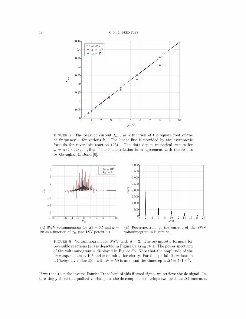
This is clearly visible in Figure 8, where only the odd harmonics of ω = 2π are present inthe power spectrum of the current. One can also see that the current exhibits spikes, due to thediscontinuity in the potential as was anticipated. This discontinuities make very accurate resultsjust around the potential switch difficult.

The Fourier transform contains more interesting information. As the zero frequency compo-nent is not interfering with the harmonics, we can single out the dc contribution. This is crudelydone by applying a block filter, which zeroes all but the near surrounding of the zero frequency.


0 1 2 3 4 5 6 7 8 9 100

0.05

0.1

0.15

0.2

0.25

0.3

0.35

0.4

0.45

√ω/π

I max

k0 � 1

k0 = 106

k0 = 35

Figure 7. The peak ac current Imax as a function of the square root of theac frequency ω for various k0. The linear line is provided by the asymptoticformula for reversible reaction (25). The dots depict numerical results forω = π/2, π, 2π, . . . , 64π. The linear relation is in agreement with the resultsby Gavaghan & Bond [6].

−10 −8 −6 −4 −2 0 2 4 6 8 10

−6

−4

−2

0

2

4

6

θdc

I dc

k0 = 106

k0 � 1

(a) SWV voltammogram for ∆θ = 0.5 and ω =2π as a function of θdc (the LSV potential).

0 2 4 6 8 10 12 14 16 18 200

500

1,000

1,500

2,000

2,500

3,000

3,500

4,000

ω/π

Pow

er

(b) Powerspectrum of the current of the SWVvoltammogram in Figure 8a.

Figure 8. Voltammogram for SWV with d = 2. The asymptotic formula forreversible reactions (25) is depicted in Figure 8a as k0 � 1. The power spectrumof the voltammogram is displayed in Figure 8b. Note that the amplitude of thedc component is ∼ 104 and is ommited for clarity. For the spatial discretisationa Chebyshev collocation with N = 50 is used and the timestep is ∆t = 5 ·10−5.

If we then take the inverse Fourier Transform of this filtered signal we retrieve the dc signal. In-terestingly there is a qualitative change as the dc component develops two peaks as ∆θ increases.


An explanation is offered by Oldham, Gavaghan & Bond [9]. The potential is a combination oftwo linear sweeps which are turned on alternatively. The two peaks originate from these twosweeps. They separate as ∆θ increases, one towards the positive θ direction and one towards thenegative.

−20 −15 −10 −5 0 5 10 15 200.05

0.1

0.15

0.2

0.25

0.3

θdc

I dc

∆ θ = 1∆ θ = 3∆ θ = 8

Figure 9. The dc current component for SWV as a function of θdc (the LSVpotential). Model parameters are d = 1, ω = 4π and k0 = 106. The results yieldgood agreement with Gavaghan et al. [7].

5. Conclusion

We derived a mathematical model for the dynamics of a single redox reaction, given by (5),at an electrode immersed in a liquid. Upon specification of the externally applied potential wecould derive a closed set of equations. Five specific external potentials were considered in moredetail, representing the following electrochemical techniques; chronoamperometry, linear sweepvoltammetry, cyclic voltammetry, alternating current voltammetry and square wave voltammetry.A combination of analytical expressions in the case of reversible reactions and numerics in thecase of (quasi)-reversible reactions provides a versatile way to explore common electrochemicalproblems.

The analysis set out in this paper could be easily extended in a few ways. Firstly we could lookinto the effect of more involved reaction mechanisms, as already mentioned when discussing cyclicvoltammetry. Different electrode geometries, such as a disc or a heterogeneous surface, could beanother generalisation of the results in this paper, which only discusses planar electrodes. Thismight require numerical simulations in two or three dimensions. The effect of chemical transportby means other than diffusion, such as convection, could also be considered.


Acknowledgements

We would like to thank Dr. K. Gillow for useful discussions and guidance in the project. Thiswork was carried out jointly with E. Kruger, V. Pereira and J. Williams.

Appendix A. Appendix

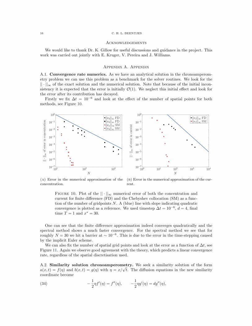
A.1. Convergence rate numerics. As we have an analytical solution in the chronoamperom-etry problem we can use this problem as a benchmark for the solver routines. We look for the|| · ||∞ of the exact solution and the numerical solution. Note that because of the initial incon-sistency it is expected that the error is initially O(1). We neglect this initial effect and look forthe error after its contribution has decayed.

Firstly we fix ∆t = 10−6 and look at the effect of the number of spatial points for bothmethods, see Figure 10.

101 102 10310−7

10−6

10−5

10−4

10−3

10−2

10−1

100

N

||·|| ∞

ofer

ror

inco

nce

ntra

tion

||eb||∞ FD||eb||∞ FD||ea||∞ SM||eb||∞ SM

(a) Error in the numerical approximation of theconcentration.

100 101 102 103 10410−7

10−6

10−5

10−4

10−3

10−2

10−1

100

N

||·|| ∞

ofer

ror

incu

rren

t

||eI ||∞ FD||eI ||∞ SM

(b) Error in the numerical approximation of the cur-rent.

Figure 10. Plot of the || · ||∞ numerical error of both the concentration andcurrent for finite difference (FD) and the Chebyshev collocation (SM) as a func-tion of the number of gridpoints N . A (blue) line with slope indicating quadraticconvergence is plotted as a reference. We used timestep ∆t = 10−6, d = 4, finaltime T = 1 and x∗ = 30.

One can see that the finite difference approximation indeed converges quadratically and thespectral method shows a much faster convergence. For the spectral method we see that forroughly N = 30 we hit a barrier at ∼ 10−6. This is due to the error in the time-stepping causedby the implicit Euler scheme.

We can also fix the number of spatial grid points and look at the error as a function of ∆t, seeFigure 11. Again we observe good agreement with the theory, which predicts a linear convergencerate, regardless of the spatial discretisation used.

A.2. Similarity solution chronoamperometry. We seek a similarity solution of the forma(x, t) = f(η) and b(x, t) = g(η) with η = x/

√t. The diffusion equations in the new similarity

coordinate become

(34) − 1

2ηf ′(η) = f ′′(η), −1

2ηg′(η) = dg′′(η),


10−5 10−4 10−3 10−2 10−110−5

10−4

10−3

10−2

10−1

∆t

||·|| ∞

ofer

ror

inco

nce

ntra

tion

||ea||∞ FD||eb||∞ FD||ea||∞ SM||eb||∞ SM

(a) Error in the numerical approximation of theconcentration.

10−5 10−4 10−3 10−2 10−110−5

10−4

10−3

10−2

10−1

∆t

||·|| ∞

ofer

ror

inco

nce

ntra

tion

||eI ||∞ FD||ea||∞ SM

(b) Error in the numerical approximation of thecurrent.

Figure 11. Plot of the || · ||∞ numerical error of both the concentration andcurrent for finite difference (FD) and the Chebyshev collocation (SM) as a func-tion of the timestep ∆t. A (blue) line with slope indicating linear convergenceis plotted as a reference. We used timestep NFD = 2000, NSM = 30, d = 4, finaltime T = 1 and x∗ = 30.

with ′ = ddη . These ODEs for f and g can be explicitly integrated to give

(35) f(η) = c1erf(η/2) + c2, g(η) = c3erf(η/2√d) + c4.

The integration constants ci are determined by the boundary conditions (12d-12e,20)

(36) 1 = c1 + c2, 0 = c3 + c4, c2 = c4e−θ, c1 = −

√dc3.

Note that in order to have a valid similarity solution we need that θ = constant to make theboundary conditions consistent with the similarity variable. Solving for the integration constantsone finds (21a,21b).

A.3. Current for reversible reactions. We consider the problem (12a-12g), where insteadof (12e) we work with the Nernst-equation (20) at the electrode-liquid interface because of thereversibility of the reaction (k0 � 1).

Now we take the Laplace transform of a and b with respect to t

(37) A(x, s) = L[a(x, t); t], B(x, s) = L[b(x, t); t].

We use the boundary conditions and the properties of the Laplace transform to find

(38) L[at(x, t); t] = sA(x, s)− 1, L[bt(x, t); t] = sB(x, s).

The diffusion equations for a and b consequently transform to

∂2A

∂x2= sA(x, s)− 1,(39a)

d∂2B

∂x2= sB(x, s),(39b)


which is supplemented by Laplace transforms of the boundary conditions

A→ 1

s, B → 0, as x→∞,(40a)

∂A

∂x+ d

∂B

∂x= 0, at x = 0,(40b)

A(0, s) = L[e−θ(t)b(0, t)

].(40c)

These equations can be solved and this yields

(41) A(x, s) =

(A(0, s)− 1

s

)e−√sx +

1

s, B(x, s) = B(0, s)e−

√sx/√d.

Note that (40b,41) together with (40c) gives

(42) −√s

(L[e−θ(t)b(0, t)

]− 1

s

)=∂A

∂x

∣∣∣∣x=0

= −d ∂B∂x

∣∣∣∣x=0

=√sdL [b(0, t)] .

This can be solved for b(0, t) (and thus a(0, t) as well) by taking the inverse Laplace transformon both side and using linearity

(43) b(0, t) =eθ(t)√

deθ(t) + 1, a(0, t) =

1√deθ(t) + 1

,

generalising for non-constant θ the chronoamperometry boundary conditions.Finally, since I(t) = ax(0, t) we find upon taking its Laplace transform

(44) L[I(t)] =∂A

∂x

∣∣∣∣x=0

=√sdL [b(0, t)] .

This then yields that

(45)

√π√sL[I(t)] =

√dπL [b(0, t)] ,

which we can transform back to original coordinates by taking the inverse Laplace transform.Note then that L(1/

√t) =

√π/√s. Upon using b(0, t) and using the convolution theorem for the

Laplace transform this gives

(46)

√dπeθ(t)√deθ(t) + 1

= I(t) ∗ L−1

[√π√s

]= I(t) ∗ 1√

t.

This finally yields the desired implicit relation for the current

(47) F (t) =

√dπ√

d+ e−θ(t)=

∫ t

0

I(τ)√t− τ

dτ.

A.3.1. Numerical approximation integral. Two ways are proposed to circumvent the divergenceof the integrand. Firstly we can use an integration by parts to find

F (t) =

∫ t

0

I(τ)√t− τ

dτ = −2I(τ)√t− τ

∣∣t0

+ 2

∫ t

0

I ′(τ)√t− τ dτ,

= −2I(0)√t+ 2

∫ t

0


= 2

∫ t

0

I ′(τ)√t− τ dτ.(48)


This removed the singularity of the integrand at the cost of replacing I(t) by its time-derivative.Another method accomplishes a similar result, but without replacing I(t) by a derivative. Thisis achieved by integrating the implicit current integral

G(t) =

∫ t

0

F (s) ds =

∫ t

0

∫ s

0

I(τ)√s− τ

dτ ds,

=

∫ t

0

∫ t

τ

I(τ)√s− τ

dsdτ,

= 2

∫ t

0

I(τ)√t− τ dτ.(49)

As mentioned in the paper the numerical approximation relies on approximation of integralsof the form

(50)

∫ ti+1

ti


∫ ti+1

ti

I(τ)√t− τ dτ.

Here we will only describe four closely related quadrature methods.The first method, applicable to both integrals, is the midpoint-approximation. This method

approximates the integral by the area of a rectangle whose height is determined by the integrandvalue at the midpoint of the integration domain∫ ti+1

ti

I ′(τ)√n∆t− τ dτ ≈ ∆tI ′(ti+ 1

2)√

∆t

√n− i− 1

2≈ (Ii+1 − Ii)

√n− i− 1

2

√∆t,(51a) ∫ ti+1

ti

I(τ)√n∆t− τ dτ ≈ ∆tI(ti+ 1

2)√

∆t

√n− i− 1

2(51b)

where we have used I ′(ti+ 12) ≈ (Ii+1 − Ii)/∆t, the central approximation of the first derivative.

The other methods use a partial midpoint method, namely assuming that I ′(τ) = I ′(ti+ 12)

over the integration, to give

(52)

∫ ti+1

ti

I ′(τ)√n∆t− τ dτ ≈ I ′(ti+ 1

2)

∫ ti+1

ti

√n∆t− τ dτ.

The last integral can be either calculated exactly to yield∫ ti+1

ti

I ′(τ)√n∆t− τ dτ ≈ 2

3(Ii+1 − Ii)

√∆t(

(n− i) 32 − (n− i− 1)

32

),(53)

or approximated by use of the trapezium rule∫ ti+1

ti

I ′(τ)√n∆t− τ dτ ≈ 1

2(Ii+1 − Ii)

√∆t(

(n− i− 1)12 + (n− i) 1

2

).(54)

We note that all approximations are indeed of the form (28) for different constants pi. Thisyields the approximations

F (n∆t) ≈ 2√

∆t

n−1∑i=0

pi (Ii+1 − Ii) = 2√

∆t

(pn−1In +

n−1∑i=1

(pi−1 − pi)Ii − p0I0

),(55a)

G(n∆t) ≈ 2∆t√

∆t

n−1∑i=0

(√n− i− 1

2

)I(ti+ 1

2).(55b)


This can be rewritten to find In as a function of the current at the previous times

In ≈1

pn−1

(F (n∆t)

2√

∆t+ p0I0 −

n−1∑i=1

(pi−1 − pi)Ii

),(56a)

In− 12≈√

2

(G(n∆t)

2∆t√

∆t+

n−2∑i=0

(√n− i− 1

2

)Ii+ 1

2

).(56b)

A final note can be made on the cost of the approximation. It appears that the methodsthat work with F (t) instead of G(t) are more advantageous, as they do not require an extraintegration. In the case of LSV however the integral G(t) can be calculated explicitly

(57) G(t) =

∫ t

0

F (s) ds =

∫ t

0

√dπ√

d+ e−θ0−sds =

√π log

(e−θ0 + et

√d

e−θ0 +√d

),

which puts the method on equal scale with the other methods.The methods could be slow if implemented naively, where at every iteration we need to compute

an increasing number of coefficients and sum those. A significant speed-up can be achieved ifthese coefficients are initially vectorised so that we only have to compute them once. We thencan code the summation over all previous Ii as a vector-vector product so that the cost of everynew time step is just roughly a vector-vector product.

REFERENCES 21

References

1. Bard, A. J. & Faulkner, L. R. Electrochemical Methods: Fundamentals and Applications(Wiley, 2000).

2. Butler, J. A. V. Studies in heterogeneous equilibria. Part II. The kinetic interpretation ofthe nernst theory of electromotive force. Transactions of the Faraday Society 19, 729 (1924).

3. Compton, R. G., Laborda, E. & Ward, K. Understanding Voltammetry (Imperial CollegePress, 2014).

4. Engblom, S. O., Myland, J. C. & Oldham, K. B. Must ac voltammetry employ small signals?Journal of Electroanalytical Chemistry 480, 120–132 (2000).

5. Erdey-Gruz, T. & Volmer, M. Zur theorie der wasserstoffuberspannung. Z. Phys. Chem. A150, 203 (1930).

6. Gavaghan, D. & Bond, A. A complete numerical simulation of the techniques of alternatingcurrent linear sweep and cyclic voltammetry: analysis of a reversible process by conventionaland fast Fourier transform methods. Journal of Electroanalytical Chemistry 480, 133–149(2000).

7. Gavaghan, D., Elton, D., Oldham, K. & Bond, A. Analysis of ramped square-wave voltam-metry in the frequency domain. Journal of Electroanalytical Chemistry 512, 1–15 (2001).

8. Hundsdorfer, W. & Verwer, J. G. Numerical Solution of Time-Dependent Advection-Diffusion-Reaction Equations (Springer Science & Business Media, 2003).

9. Oldham, K. B., Gavaghan, D. J. & Bond, A. M. A Full Analytic Treatment of ReversibleLinear-Scan Voltammetry with Square-Wave Modulation. The Journal of Physical Chem-istry B 106, 152–157 (2002).

10. Trefethen, L. N. Spectral Methods in MATLAB (Society for Industrial and Applied Math-ematics, 2000).

introduction - university of oxfordpeople.maths.ox.ac.uk/beentjes/essays/computational... · range...

Documents