IntroductionThis manual contains complete documentation for Ultra Fractal 6 in printer-friendly format. All information in this manual isalso accessible from the Help menu in Ultra Fractal. On Windows, you can also get context-sensitive help in every dialogand tool window in Ultra Fractal. Click the ? button in the title bar, and then click on a control to learn more about it.

The compiler reference is not included in this manual because it would make it unnecessary large. To access the compilerreference, click Contents on the Help menu in Ultra Fractal. In the Writing Formulas chapter, there is an additionalReference chapter that lists all built-in functions, operators, keywords, and so on. Alternatively, click on a symbol in theformula editor and then click Help on the Help menu.

Table of Contents

. . . . . . . . . . . . . . . . . . . . . . . . . . . . . . . . . . . . . . . . . . . . . . . . . . . . . . . . . . . . . . . . . . . . . . . . . . . . . . . . . . . . . . . 10

. . . . . . . . . . . . . . . . . . . . . . . . . . . . . . . . . . . . . . . . . . . . . . . . . . . . . . . . . . . . . . . . . . . . . . . . . . . . . . . . . . . . . . . 12

. . . . . . . . . . . . . . . . . . . . . . . . . . . . . . . . . . . . . . . . . . . . . . . . . . . . . . . . . . . . . . . . . . . . . . . . . . . . . . . . . . . . . . . 13

. . . . . . . . . . . . . . . . . . . . . . . . . . . . . . . . . . . . . . . . . . . . . . . . . . . . . . . . . . . . . . . . . . . . . . . . . . . . . . . . . . . . . . . 14

. . . . . . . . . . . . . . . . . . . . . . . . . . . . . . . . . . . . . . . . . . . . . . . . . . . . . . . . . . . . . . . . . . . . . . . . . . . . . . . . . . . . . . . 15

. . . . . . . . . . . . . . . . . . . . . . . . . . . . . . . . . . . . . . . . . . . . . . . . . . . . . . . . . . . . . . . . . . . . . . . . . . . . . . . . . . . . . . . 16

. . . . . . . . . . . . . . . . . . . . . . . . . . . . . . . . . . . . . . . . . . . . . . . . . . . . . . . . . . . . . . . . . . . . . . . . . . . . . . . . . . . . . . . 17

. . . . . . . . . . . . . . . . . . . . . . . . . . . . . . . . . . . . . . . . . . . . . . . . . . . . . . . . . . . . . . . . . . . . . . . . . . . . . . . . . . . . . . . 18

. . . . . . . . . . . . . . . . . . . . . . . . . . . . . . . . . . . . . . . . . . . . . . . . . . . . . . . . . . . . . . . . . . . . . . . . . . . . . . . . . . . . . . . 19

. . . . . . . . . . . . . . . . . . . . . . . . . . . . . . . . . . . . . . . . . . . . . . . . . . . . . . . . . . . . . . . . . . . . . . . . . . . . . . . . . . . . . . . 20

. . . . . . . . . . . . . . . . . . . . . . . . . . . . . . . . . . . . . . . . . . . . . . . . . . . . . . . . . . . . . . . . . . . . . . . . . . . . . . . . . . . . . . . 21

. . . . . . . . . . . . . . . . . . . . . . . . . . . . . . . . . . . . . . . . . . . . . . . . . . . . . . . . . . . . . . . . . . . . . . . . . . . . . . . . . . . . . . . 22

. . . . . . . . . . . . . . . . . . . . . . . . . . . . . . . . . . . . . . . . . . . . . . . . . . . . . . . . . . . . . . . . . . . . . . . . . . . . . . . . . . . . . . . 23

. . . . . . . . . . . . . . . . . . . . . . . . . . . . . . . . . . . . . . . . . . . . . . . . . . . . . . . . . . . . . . . . . . . . . . . . . . . . . . . . . . . . . . . 24

. . . . . . . . . . . . . . . . . . . . . . . . . . . . . . . . . . . . . . . . . . . . . . . . . . . . . . . . . . . . . . . . . . . . . . . . . . . . . . . . . . . . . . . 25

. . . . . . . . . . . . . . . . . . . . . . . . . . . . . . . . . . . . . . . . . . . . . . . . . . . . . . . . . . . . . . . . . . . . . . . . . . . . . . . . . . . . . . . 26

. . . . . . . . . . . . . . . . . . . . . . . . . . . . . . . . . . . . . . . . . . . . . . . . . . . . . . . . . . . . . . . . . . . . . . . . . . . . . . . . . . . . . . . 27

. . . . . . . . . . . . . . . . . . . . . . . . . . . . . . . . . . . . . . . . . . . . . . . . . . . . . . . . . . . . . . . . . . . . . . . . . . . . . . . . . . . . . . . 28

. . . . . . . . . . . . . . . . . . . . . . . . . . . . . . . . . . . . . . . . . . . . . . . . . . . . . . . . . . . . . . . . . . . . . . . . . . . . . . . . . . . . . . . 29

. . . . . . . . . . . . . . . . . . . . . . . . . . . . . . . . . . . . . . . . . . . . . . . . . . . . . . . . . . . . . . . . . . . . . . . . . . . . . . . . . . . . . . . 30

. . . . . . . . . . . . . . . . . . . . . . . . . . . . . . . . . . . . . . . . . . . . . . . . . . . . . . . . . . . . . . . . . . . . . . . . . . . . . . . . . . . . . . . 31

. . . . . . . . . . . . . . . . . . . . . . . . . . . . . . . . . . . . . . . . . . . . . . . . . . . . . . . . . . . . . . . . . . . . . . . . . . . . . . . . . . . . . . . 32

. . . . . . . . . . . . . . . . . . . . . . . . . . . . . . . . . . . . . . . . . . . . . . . . . . . . . . . . . . . . . . . . . . . . . . . . . . . . . . . . . . . . . . . 33

. . . . . . . . . . . . . . . . . . . . . . . . . . . . . . . . . . . . . . . . . . . . . . . . . . . . . . . . . . . . . . . . . . . . . . . . . . . . . . . . . . . . . . . 34

. . . . . . . . . . . . . . . . . . . . . . . . . . . . . . . . . . . . . . . . . . . . . . . . . . . . . . . . . . . . . . . . . . . . . . . . . . . . . . . . . . . . . . . 35

. . . . . . . . . . . . . . . . . . . . . . . . . . . . . . . . . . . . . . . . . . . . . . . . . . . . . . . . . . . . . . . . . . . . . . . . . . . . . . . . . . . . . . . 36

. . . . . . . . . . . . . . . . . . . . . . . . . . . . . . . . . . . . . . . . . . . . . . . . . . . . . . . . . . . . . . . . . . . . . . . . . . . . . . . . . . . . . . . 37

. . . . . . . . . . . . . . . . . . . . . . . . . . . . . . . . . . . . . . . . . . . . . . . . . . . . . . . . . . . . . . . . . . . . . . . . . . . . . . . . . . . . . . . 38

. . . . . . . . . . . . . . . . . . . . . . . . . . . . . . . . . . . . . . . . . . . . . . . . . . . . . . . . . . . . . . . . . . . . . . . . . . . . . . . . . . . . . . . 39

. . . . . . . . . . . . . . . . . . . . . . . . . . . . . . . . . . . . . . . . . . . . . . . . . . . . . . . . . . . . . . . . . . . . . . . . . . . . . . . . . . . . . . . 40

. . . . . . . . . . . . . . . . . . . . . . . . . . . . . . . . . . . . . . . . . . . . . . . . . . . . . . . . . . . . . . . . . . . . . . . . . . . . . . . . . . . . . . . 41

. . . . . . . . . . . . . . . . . . . . . . . . . . . . . . . . . . . . . . . . . . . . . . . . . . . . . . . . . . . . . . . . . . . . . . . . . . . . . . . . . . . . . . . 42

. . . . . . . . . . . . . . . . . . . . . . . . . . . . . . . . . . . . . . . . . . . . . . . . . . . . . . . . . . . . . . . . . . . . . . . . . . . . . . . . . . . . . . . 43

Table of Contents

What's new?What's new in Ultra Fractal 6?

Compiler changes

Getting helpGetting help

Context-sensitive help

Help for formula authors

TutorialsTutorials

Quick Start TutorialCreating a fractal image

Changing formula parameters

Applying a coloring algorithm

Saving your fractal

Opening your saved fractal

Learning basic skillsLearning basic skills

Learning to use Switch Mode

Using the Explore tool

Synchronizing the Julia Seed

Zooming into the image

Synchronizing the location

Adding outside coloring

Working with the gradient

Synchronizing colors and Saving the image

Working with layersWorking with layers

Coloring the new layer

Editing the gradient

Learning about layer opacity

Learning about merge modes

Adding a third layer

Transparency in the gradient

Adding control points

Learning about transformationsLearning about transformations

Using the Kaleidoscope transformation

Using 3D Mapping

Twist transformation

Mapping a sphere

. . . . . . . . . . . . . . . . . . . . . . . . . . . . . . . . . . . . . . . . . . . . . . . . . . . . . . . . . . . . . . . . . . . . . . . . . . . . . . . . . . . . . . . 44

. . . . . . . . . . . . . . . . . . . . . . . . . . . . . . . . . . . . . . . . . . . . . . . . . . . . . . . . . . . . . . . . . . . . . . . . . . . . . . . . . . . . . . . 45

. . . . . . . . . . . . . . . . . . . . . . . . . . . . . . . . . . . . . . . . . . . . . . . . . . . . . . . . . . . . . . . . . . . . . . . . . . . . . . . . . . . . . . . 46

. . . . . . . . . . . . . . . . . . . . . . . . . . . . . . . . . . . . . . . . . . . . . . . . . . . . . . . . . . . . . . . . . . . . . . . . . . . . . . . . . . . . . . . 47

. . . . . . . . . . . . . . . . . . . . . . . . . . . . . . . . . . . . . . . . . . . . . . . . . . . . . . . . . . . . . . . . . . . . . . . . . . . . . . . . . . . . . . . 48

. . . . . . . . . . . . . . . . . . . . . . . . . . . . . . . . . . . . . . . . . . . . . . . . . . . . . . . . . . . . . . . . . . . . . . . . . . . . . . . . . . . . . . . 49

. . . . . . . . . . . . . . . . . . . . . . . . . . . . . . . . . . . . . . . . . . . . . . . . . . . . . . . . . . . . . . . . . . . . . . . . . . . . . . . . . . . . . . . 50

. . . . . . . . . . . . . . . . . . . . . . . . . . . . . . . . . . . . . . . . . . . . . . . . . . . . . . . . . . . . . . . . . . . . . . . . . . . . . . . . . . . . . . . 51

. . . . . . . . . . . . . . . . . . . . . . . . . . . . . . . . . . . . . . . . . . . . . . . . . . . . . . . . . . . . . . . . . . . . . . . . . . . . . . . . . . . . . . . 53

. . . . . . . . . . . . . . . . . . . . . . . . . . . . . . . . . . . . . . . . . . . . . . . . . . . . . . . . . . . . . . . . . . . . . . . . . . . . . . . . . . . . . . . 54

. . . . . . . . . . . . . . . . . . . . . . . . . . . . . . . . . . . . . . . . . . . . . . . . . . . . . . . . . . . . . . . . . . . . . . . . . . . . . . . . . . . . . . . 55

. . . . . . . . . . . . . . . . . . . . . . . . . . . . . . . . . . . . . . . . . . . . . . . . . . . . . . . . . . . . . . . . . . . . . . . . . . . . . . . . . . . . . . . 57

. . . . . . . . . . . . . . . . . . . . . . . . . . . . . . . . . . . . . . . . . . . . . . . . . . . . . . . . . . . . . . . . . . . . . . . . . . . . . . . . . . . . . . . 59

. . . . . . . . . . . . . . . . . . . . . . . . . . . . . . . . . . . . . . . . . . . . . . . . . . . . . . . . . . . . . . . . . . . . . . . . . . . . . . . . . . . . . . . 60

. . . . . . . . . . . . . . . . . . . . . . . . . . . . . . . . . . . . . . . . . . . . . . . . . . . . . . . . . . . . . . . . . . . . . . . . . . . . . . . . . . . . . . . 61

. . . . . . . . . . . . . . . . . . . . . . . . . . . . . . . . . . . . . . . . . . . . . . . . . . . . . . . . . . . . . . . . . . . . . . . . . . . . . . . . . . . . . . . 62

. . . . . . . . . . . . . . . . . . . . . . . . . . . . . . . . . . . . . . . . . . . . . . . . . . . . . . . . . . . . . . . . . . . . . . . . . . . . . . . . . . . . . . . 63

. . . . . . . . . . . . . . . . . . . . . . . . . . . . . . . . . . . . . . . . . . . . . . . . . . . . . . . . . . . . . . . . . . . . . . . . . . . . . . . . . . . . . . . 64

. . . . . . . . . . . . . . . . . . . . . . . . . . . . . . . . . . . . . . . . . . . . . . . . . . . . . . . . . . . . . . . . . . . . . . . . . . . . . . . . . . . . . . . 65

. . . . . . . . . . . . . . . . . . . . . . . . . . . . . . . . . . . . . . . . . . . . . . . . . . . . . . . . . . . . . . . . . . . . . . . . . . . . . . . . . . . . . . . 66

. . . . . . . . . . . . . . . . . . . . . . . . . . . . . . . . . . . . . . . . . . . . . . . . . . . . . . . . . . . . . . . . . . . . . . . . . . . . . . . . . . . . . . . 67

. . . . . . . . . . . . . . . . . . . . . . . . . . . . . . . . . . . . . . . . . . . . . . . . . . . . . . . . . . . . . . . . . . . . . . . . . . . . . . . . . . . . . . . 68

. . . . . . . . . . . . . . . . . . . . . . . . . . . . . . . . . . . . . . . . . . . . . . . . . . . . . . . . . . . . . . . . . . . . . . . . . . . . . . . . . . . . . . . 69

. . . . . . . . . . . . . . . . . . . . . . . . . . . . . . . . . . . . . . . . . . . . . . . . . . . . . . . . . . . . . . . . . . . . . . . . . . . . . . . . . . . . . . . 70

. . . . . . . . . . . . . . . . . . . . . . . . . . . . . . . . . . . . . . . . . . . . . . . . . . . . . . . . . . . . . . . . . . . . . . . . . . . . . . . . . . . . . . . 71

. . . . . . . . . . . . . . . . . . . . . . . . . . . . . . . . . . . . . . . . . . . . . . . . . . . . . . . . . . . . . . . . . . . . . . . . . . . . . . . . . . . . . . . 72

. . . . . . . . . . . . . . . . . . . . . . . . . . . . . . . . . . . . . . . . . . . . . . . . . . . . . . . . . . . . . . . . . . . . . . . . . . . . . . . . . . . . . . . 73

. . . . . . . . . . . . . . . . . . . . . . . . . . . . . . . . . . . . . . . . . . . . . . . . . . . . . . . . . . . . . . . . . . . . . . . . . . . . . . . . . . . . . . . 74

. . . . . . . . . . . . . . . . . . . . . . . . . . . . . . . . . . . . . . . . . . . . . . . . . . . . . . . . . . . . . . . . . . . . . . . . . . . . . . . . . . . . . . . 75

. . . . . . . . . . . . . . . . . . . . . . . . . . . . . . . . . . . . . . . . . . . . . . . . . . . . . . . . . . . . . . . . . . . . . . . . . . . . . . . . . . . . . . . 76

. . . . . . . . . . . . . . . . . . . . . . . . . . . . . . . . . . . . . . . . . . . . . . . . . . . . . . . . . . . . . . . . . . . . . . . . . . . . . . . . . . . . . . . 77

. . . . . . . . . . . . . . . . . . . . . . . . . . . . . . . . . . . . . . . . . . . . . . . . . . . . . . . . . . . . . . . . . . . . . . . . . . . . . . . . . . . . . . . 78

. . . . . . . . . . . . . . . . . . . . . . . . . . . . . . . . . . . . . . . . . . . . . . . . . . . . . . . . . . . . . . . . . . . . . . . . . . . . . . . . . . . . . . . 79

. . . . . . . . . . . . . . . . . . . . . . . . . . . . . . . . . . . . . . . . . . . . . . . . . . . . . . . . . . . . . . . . . . . . . . . . . . . . . . . . . . . . . . . 80

. . . . . . . . . . . . . . . . . . . . . . . . . . . . . . . . . . . . . . . . . . . . . . . . . . . . . . . . . . . . . . . . . . . . . . . . . . . . . . . . . . . . . . . 81

. . . . . . . . . . . . . . . . . . . . . . . . . . . . . . . . . . . . . . . . . . . . . . . . . . . . . . . . . . . . . . . . . . . . . . . . . . . . . . . . . . . . . . . 82

. . . . . . . . . . . . . . . . . . . . . . . . . . . . . . . . . . . . . . . . . . . . . . . . . . . . . . . . . . . . . . . . . . . . . . . . . . . . . . . . . . . . . . . 83

. . . . . . . . . . . . . . . . . . . . . . . . . . . . . . . . . . . . . . . . . . . . . . . . . . . . . . . . . . . . . . . . . . . . . . . . . . . . . . . . . . . . . . . 84

. . . . . . . . . . . . . . . . . . . . . . . . . . . . . . . . . . . . . . . . . . . . . . . . . . . . . . . . . . . . . . . . . . . . . . . . . . . . . . . . . . . . . . . 85

. . . . . . . . . . . . . . . . . . . . . . . . . . . . . . . . . . . . . . . . . . . . . . . . . . . . . . . . . . . . . . . . . . . . . . . . . . . . . . . . . . . . . . . 86

Adding a frame

Zooming with multiple layers

Using the Clipping transformation

Exporting the image

MaskingIntroduction to masking

Layer 2 - Waves Trap

Layer 3 - Box Trap

Fine-tuning the gradient

Layer 4 - Gaussian Integer

Adding a mask layer

Editing the mask

Rendering the image

Some final thoughts

Working with animationsWorking with animations

Making a zoom movie

Playing the movie

Experimenting with Animate mode

Extending the animation

Using the Timeline tool window

Adding gradient animation

Adding a new layer

Rendering the animation

About fractalsWhat are fractals?

Self-similarity

Julia sets

The Mandelbrot set

Fractals today

Where to start

WorkspaceWorkspace overview

Working with tool windows

Tool windows overview

Layer Properties tool window

Fractal Properties tool window

Fractal Mode tool window

Statistics tool window

Color cycling tool window

Network tool window

Render to Disk tool window

Compiler Messages tool window

Options dialog

. . . . . . . . . . . . . . . . . . . . . . . . . . . . . . . . . . . . . . . . . . . . . . . . . . . . . . . . . . . . . . . . . . . . . . . . . . . . . . . . . . . . . . . 87

. . . . . . . . . . . . . . . . . . . . . . . . . . . . . . . . . . . . . . . . . . . . . . . . . . . . . . . . . . . . . . . . . . . . . . . . . . . . . . . . . . . . . . . 88

. . . . . . . . . . . . . . . . . . . . . . . . . . . . . . . . . . . . . . . . . . . . . . . . . . . . . . . . . . . . . . . . . . . . . . . . . . . . . . . . . . . . . . . 89

. . . . . . . . . . . . . . . . . . . . . . . . . . . . . . . . . . . . . . . . . . . . . . . . . . . . . . . . . . . . . . . . . . . . . . . . . . . . . . . . . . . . . . . 90

. . . . . . . . . . . . . . . . . . . . . . . . . . . . . . . . . . . . . . . . . . . . . . . . . . . . . . . . . . . . . . . . . . . . . . . . . . . . . . . . . . . . . . . 91

. . . . . . . . . . . . . . . . . . . . . . . . . . . . . . . . . . . . . . . . . . . . . . . . . . . . . . . . . . . . . . . . . . . . . . . . . . . . . . . . . . . . . . . 92

. . . . . . . . . . . . . . . . . . . . . . . . . . . . . . . . . . . . . . . . . . . . . . . . . . . . . . . . . . . . . . . . . . . . . . . . . . . . . . . . . . . . . . . 93

. . . . . . . . . . . . . . . . . . . . . . . . . . . . . . . . . . . . . . . . . . . . . . . . . . . . . . . . . . . . . . . . . . . . . . . . . . . . . . . . . . . . . . . 94

. . . . . . . . . . . . . . . . . . . . . . . . . . . . . . . . . . . . . . . . . . . . . . . . . . . . . . . . . . . . . . . . . . . . . . . . . . . . . . . . . . . . . . . 95

. . . . . . . . . . . . . . . . . . . . . . . . . . . . . . . . . . . . . . . . . . . . . . . . . . . . . . . . . . . . . . . . . . . . . . . . . . . . . . . . . . . . . . . 96

. . . . . . . . . . . . . . . . . . . . . . . . . . . . . . . . . . . . . . . . . . . . . . . . . . . . . . . . . . . . . . . . . . . . . . . . . . . . . . . . . . . . . . . 97

. . . . . . . . . . . . . . . . . . . . . . . . . . . . . . . . . . . . . . . . . . . . . . . . . . . . . . . . . . . . . . . . . . . . . . . . . . . . . . . . . . . . . . . 98

. . . . . . . . . . . . . . . . . . . . . . . . . . . . . . . . . . . . . . . . . . . . . . . . . . . . . . . . . . . . . . . . . . . . . . . . . . . . . . . . . . . . . . . 99

. . . . . . . . . . . . . . . . . . . . . . . . . . . . . . . . . . . . . . . . . . . . . . . . . . . . . . . . . . . . . . . . . . . . . . . . . . . . . . . . . . . . . . . 100

. . . . . . . . . . . . . . . . . . . . . . . . . . . . . . . . . . . . . . . . . . . . . . . . . . . . . . . . . . . . . . . . . . . . . . . . . . . . . . . . . . . . . . . 101

. . . . . . . . . . . . . . . . . . . . . . . . . . . . . . . . . . . . . . . . . . . . . . . . . . . . . . . . . . . . . . . . . . . . . . . . . . . . . . . . . . . . . . . 102

. . . . . . . . . . . . . . . . . . . . . . . . . . . . . . . . . . . . . . . . . . . . . . . . . . . . . . . . . . . . . . . . . . . . . . . . . . . . . . . . . . . . . . . 103

. . . . . . . . . . . . . . . . . . . . . . . . . . . . . . . . . . . . . . . . . . . . . . . . . . . . . . . . . . . . . . . . . . . . . . . . . . . . . . . . . . . . . . . 104

. . . . . . . . . . . . . . . . . . . . . . . . . . . . . . . . . . . . . . . . . . . . . . . . . . . . . . . . . . . . . . . . . . . . . . . . . . . . . . . . . . . . . . . 105

. . . . . . . . . . . . . . . . . . . . . . . . . . . . . . . . . . . . . . . . . . . . . . . . . . . . . . . . . . . . . . . . . . . . . . . . . . . . . . . . . . . . . . . 106

. . . . . . . . . . . . . . . . . . . . . . . . . . . . . . . . . . . . . . . . . . . . . . . . . . . . . . . . . . . . . . . . . . . . . . . . . . . . . . . . . . . . . . . 107

. . . . . . . . . . . . . . . . . . . . . . . . . . . . . . . . . . . . . . . . . . . . . . . . . . . . . . . . . . . . . . . . . . . . . . . . . . . . . . . . . . . . . . . 108

. . . . . . . . . . . . . . . . . . . . . . . . . . . . . . . . . . . . . . . . . . . . . . . . . . . . . . . . . . . . . . . . . . . . . . . . . . . . . . . . . . . . . . . 109

. . . . . . . . . . . . . . . . . . . . . . . . . . . . . . . . . . . . . . . . . . . . . . . . . . . . . . . . . . . . . . . . . . . . . . . . . . . . . . . . . . . . . . . 110

. . . . . . . . . . . . . . . . . . . . . . . . . . . . . . . . . . . . . . . . . . . . . . . . . . . . . . . . . . . . . . . . . . . . . . . . . . . . . . . . . . . . . . . 111

. . . . . . . . . . . . . . . . . . . . . . . . . . . . . . . . . . . . . . . . . . . . . . . . . . . . . . . . . . . . . . . . . . . . . . . . . . . . . . . . . . . . . . . 112

. . . . . . . . . . . . . . . . . . . . . . . . . . . . . . . . . . . . . . . . . . . . . . . . . . . . . . . . . . . . . . . . . . . . . . . . . . . . . . . . . . . . . . . 113

. . . . . . . . . . . . . . . . . . . . . . . . . . . . . . . . . . . . . . . . . . . . . . . . . . . . . . . . . . . . . . . . . . . . . . . . . . . . . . . . . . . . . . . 114

. . . . . . . . . . . . . . . . . . . . . . . . . . . . . . . . . . . . . . . . . . . . . . . . . . . . . . . . . . . . . . . . . . . . . . . . . . . . . . . . . . . . . . . 115

. . . . . . . . . . . . . . . . . . . . . . . . . . . . . . . . . . . . . . . . . . . . . . . . . . . . . . . . . . . . . . . . . . . . . . . . . . . . . . . . . . . . . . . 116

. . . . . . . . . . . . . . . . . . . . . . . . . . . . . . . . . . . . . . . . . . . . . . . . . . . . . . . . . . . . . . . . . . . . . . . . . . . . . . . . . . . . . . . 117

. . . . . . . . . . . . . . . . . . . . . . . . . . . . . . . . . . . . . . . . . . . . . . . . . . . . . . . . . . . . . . . . . . . . . . . . . . . . . . . . . . . . . . . 118

. . . . . . . . . . . . . . . . . . . . . . . . . . . . . . . . . . . . . . . . . . . . . . . . . . . . . . . . . . . . . . . . . . . . . . . . . . . . . . . . . . . . . . . 119

. . . . . . . . . . . . . . . . . . . . . . . . . . . . . . . . . . . . . . . . . . . . . . . . . . . . . . . . . . . . . . . . . . . . . . . . . . . . . . . . . . . . . . . 120

. . . . . . . . . . . . . . . . . . . . . . . . . . . . . . . . . . . . . . . . . . . . . . . . . . . . . . . . . . . . . . . . . . . . . . . . . . . . . . . . . . . . . . . 121

. . . . . . . . . . . . . . . . . . . . . . . . . . . . . . . . . . . . . . . . . . . . . . . . . . . . . . . . . . . . . . . . . . . . . . . . . . . . . . . . . . . . . . . 122

. . . . . . . . . . . . . . . . . . . . . . . . . . . . . . . . . . . . . . . . . . . . . . . . . . . . . . . . . . . . . . . . . . . . . . . . . . . . . . . . . . . . . . . 123

. . . . . . . . . . . . . . . . . . . . . . . . . . . . . . . . . . . . . . . . . . . . . . . . . . . . . . . . . . . . . . . . . . . . . . . . . . . . . . . . . . . . . . . 124

. . . . . . . . . . . . . . . . . . . . . . . . . . . . . . . . . . . . . . . . . . . . . . . . . . . . . . . . . . . . . . . . . . . . . . . . . . . . . . . . . . . . . . . 125

. . . . . . . . . . . . . . . . . . . . . . . . . . . . . . . . . . . . . . . . . . . . . . . . . . . . . . . . . . . . . . . . . . . . . . . . . . . . . . . . . . . . . . . 126

. . . . . . . . . . . . . . . . . . . . . . . . . . . . . . . . . . . . . . . . . . . . . . . . . . . . . . . . . . . . . . . . . . . . . . . . . . . . . . . . . . . . . . . 127

Fractal windowsFractal windows

Normal mode

Select mode

Switch mode

Opening and saving fractals

Parameter files

Copying and pasting fractals

Fractal history list

Anti-aliasing (fractal window)

Full screen mode

Default fractal

Copyright and tweaking

Calculation details

GradientsGradients

How gradients work

Editing gradients

Transparent gradients

Adjusting gradients

Opening and saving gradients

Fractal formulasFractal formulas

Working with fractal formulas

Maximum iterations

Formula parameters

Explore

Eyedropper

Presets

Arbitrary precision

Perturbation calculations

Public formulas

Standard fractal formulas

Embossed (Julia, Mandelbrot, Newton)

Julia

Julia (Built-in)

Lambda (Julia, Mandelbrot)

Magnet 1 and 2 (Julia, Mandelbrot)

Mandelbrot

Mandelbrot (Built-in)

Newton

Nova (Julia, Mandelbrot)

Phoenix (Julia, Mandelbrot)

Pixel

. . . . . . . . . . . . . . . . . . . . . . . . . . . . . . . . . . . . . . . . . . . . . . . . . . . . . . . . . . . . . . . . . . . . . . . . . . . . . . . . . . . . . . . 128

. . . . . . . . . . . . . . . . . . . . . . . . . . . . . . . . . . . . . . . . . . . . . . . . . . . . . . . . . . . . . . . . . . . . . . . . . . . . . . . . . . . . . . . 129

. . . . . . . . . . . . . . . . . . . . . . . . . . . . . . . . . . . . . . . . . . . . . . . . . . . . . . . . . . . . . . . . . . . . . . . . . . . . . . . . . . . . . . . 130

. . . . . . . . . . . . . . . . . . . . . . . . . . . . . . . . . . . . . . . . . . . . . . . . . . . . . . . . . . . . . . . . . . . . . . . . . . . . . . . . . . . . . . . 131

. . . . . . . . . . . . . . . . . . . . . . . . . . . . . . . . . . . . . . . . . . . . . . . . . . . . . . . . . . . . . . . . . . . . . . . . . . . . . . . . . . . . . . . 132

. . . . . . . . . . . . . . . . . . . . . . . . . . . . . . . . . . . . . . . . . . . . . . . . . . . . . . . . . . . . . . . . . . . . . . . . . . . . . . . . . . . . . . . 133

. . . . . . . . . . . . . . . . . . . . . . . . . . . . . . . . . . . . . . . . . . . . . . . . . . . . . . . . . . . . . . . . . . . . . . . . . . . . . . . . . . . . . . . 134

. . . . . . . . . . . . . . . . . . . . . . . . . . . . . . . . . . . . . . . . . . . . . . . . . . . . . . . . . . . . . . . . . . . . . . . . . . . . . . . . . . . . . . . 135

. . . . . . . . . . . . . . . . . . . . . . . . . . . . . . . . . . . . . . . . . . . . . . . . . . . . . . . . . . . . . . . . . . . . . . . . . . . . . . . . . . . . . . . 136

. . . . . . . . . . . . . . . . . . . . . . . . . . . . . . . . . . . . . . . . . . . . . . . . . . . . . . . . . . . . . . . . . . . . . . . . . . . . . . . . . . . . . . . 137

. . . . . . . . . . . . . . . . . . . . . . . . . . . . . . . . . . . . . . . . . . . . . . . . . . . . . . . . . . . . . . . . . . . . . . . . . . . . . . . . . . . . . . . 138

. . . . . . . . . . . . . . . . . . . . . . . . . . . . . . . . . . . . . . . . . . . . . . . . . . . . . . . . . . . . . . . . . . . . . . . . . . . . . . . . . . . . . . . 139

. . . . . . . . . . . . . . . . . . . . . . . . . . . . . . . . . . . . . . . . . . . . . . . . . . . . . . . . . . . . . . . . . . . . . . . . . . . . . . . . . . . . . . . 140

. . . . . . . . . . . . . . . . . . . . . . . . . . . . . . . . . . . . . . . . . . . . . . . . . . . . . . . . . . . . . . . . . . . . . . . . . . . . . . . . . . . . . . . 141

. . . . . . . . . . . . . . . . . . . . . . . . . . . . . . . . . . . . . . . . . . . . . . . . . . . . . . . . . . . . . . . . . . . . . . . . . . . . . . . . . . . . . . . 142

. . . . . . . . . . . . . . . . . . . . . . . . . . . . . . . . . . . . . . . . . . . . . . . . . . . . . . . . . . . . . . . . . . . . . . . . . . . . . . . . . . . . . . . 143

. . . . . . . . . . . . . . . . . . . . . . . . . . . . . . . . . . . . . . . . . . . . . . . . . . . . . . . . . . . . . . . . . . . . . . . . . . . . . . . . . . . . . . . 144

. . . . . . . . . . . . . . . . . . . . . . . . . . . . . . . . . . . . . . . . . . . . . . . . . . . . . . . . . . . . . . . . . . . . . . . . . . . . . . . . . . . . . . . 145

. . . . . . . . . . . . . . . . . . . . . . . . . . . . . . . . . . . . . . . . . . . . . . . . . . . . . . . . . . . . . . . . . . . . . . . . . . . . . . . . . . . . . . . 146

. . . . . . . . . . . . . . . . . . . . . . . . . . . . . . . . . . . . . . . . . . . . . . . . . . . . . . . . . . . . . . . . . . . . . . . . . . . . . . . . . . . . . . . 147

. . . . . . . . . . . . . . . . . . . . . . . . . . . . . . . . . . . . . . . . . . . . . . . . . . . . . . . . . . . . . . . . . . . . . . . . . . . . . . . . . . . . . . . 148

. . . . . . . . . . . . . . . . . . . . . . . . . . . . . . . . . . . . . . . . . . . . . . . . . . . . . . . . . . . . . . . . . . . . . . . . . . . . . . . . . . . . . . . 149

. . . . . . . . . . . . . . . . . . . . . . . . . . . . . . . . . . . . . . . . . . . . . . . . . . . . . . . . . . . . . . . . . . . . . . . . . . . . . . . . . . . . . . . 150

. . . . . . . . . . . . . . . . . . . . . . . . . . . . . . . . . . . . . . . . . . . . . . . . . . . . . . . . . . . . . . . . . . . . . . . . . . . . . . . . . . . . . . . 151

. . . . . . . . . . . . . . . . . . . . . . . . . . . . . . . . . . . . . . . . . . . . . . . . . . . . . . . . . . . . . . . . . . . . . . . . . . . . . . . . . . . . . . . 153

. . . . . . . . . . . . . . . . . . . . . . . . . . . . . . . . . . . . . . . . . . . . . . . . . . . . . . . . . . . . . . . . . . . . . . . . . . . . . . . . . . . . . . . 154

. . . . . . . . . . . . . . . . . . . . . . . . . . . . . . . . . . . . . . . . . . . . . . . . . . . . . . . . . . . . . . . . . . . . . . . . . . . . . . . . . . . . . . . 155

. . . . . . . . . . . . . . . . . . . . . . . . . . . . . . . . . . . . . . . . . . . . . . . . . . . . . . . . . . . . . . . . . . . . . . . . . . . . . . . . . . . . . . . 156

. . . . . . . . . . . . . . . . . . . . . . . . . . . . . . . . . . . . . . . . . . . . . . . . . . . . . . . . . . . . . . . . . . . . . . . . . . . . . . . . . . . . . . . 157

. . . . . . . . . . . . . . . . . . . . . . . . . . . . . . . . . . . . . . . . . . . . . . . . . . . . . . . . . . . . . . . . . . . . . . . . . . . . . . . . . . . . . . . 158

. . . . . . . . . . . . . . . . . . . . . . . . . . . . . . . . . . . . . . . . . . . . . . . . . . . . . . . . . . . . . . . . . . . . . . . . . . . . . . . . . . . . . . . 159

. . . . . . . . . . . . . . . . . . . . . . . . . . . . . . . . . . . . . . . . . . . . . . . . . . . . . . . . . . . . . . . . . . . . . . . . . . . . . . . . . . . . . . . 160

. . . . . . . . . . . . . . . . . . . . . . . . . . . . . . . . . . . . . . . . . . . . . . . . . . . . . . . . . . . . . . . . . . . . . . . . . . . . . . . . . . . . . . . 161

. . . . . . . . . . . . . . . . . . . . . . . . . . . . . . . . . . . . . . . . . . . . . . . . . . . . . . . . . . . . . . . . . . . . . . . . . . . . . . . . . . . . . . . 162

. . . . . . . . . . . . . . . . . . . . . . . . . . . . . . . . . . . . . . . . . . . . . . . . . . . . . . . . . . . . . . . . . . . . . . . . . . . . . . . . . . . . . . . 163

. . . . . . . . . . . . . . . . . . . . . . . . . . . . . . . . . . . . . . . . . . . . . . . . . . . . . . . . . . . . . . . . . . . . . . . . . . . . . . . . . . . . . . . 164

. . . . . . . . . . . . . . . . . . . . . . . . . . . . . . . . . . . . . . . . . . . . . . . . . . . . . . . . . . . . . . . . . . . . . . . . . . . . . . . . . . . . . . . 165

. . . . . . . . . . . . . . . . . . . . . . . . . . . . . . . . . . . . . . . . . . . . . . . . . . . . . . . . . . . . . . . . . . . . . . . . . . . . . . . . . . . . . . . 166

. . . . . . . . . . . . . . . . . . . . . . . . . . . . . . . . . . . . . . . . . . . . . . . . . . . . . . . . . . . . . . . . . . . . . . . . . . . . . . . . . . . . . . . 167

. . . . . . . . . . . . . . . . . . . . . . . . . . . . . . . . . . . . . . . . . . . . . . . . . . . . . . . . . . . . . . . . . . . . . . . . . . . . . . . . . . . . . . . 168

. . . . . . . . . . . . . . . . . . . . . . . . . . . . . . . . . . . . . . . . . . . . . . . . . . . . . . . . . . . . . . . . . . . . . . . . . . . . . . . . . . . . . . . 169

. . . . . . . . . . . . . . . . . . . . . . . . . . . . . . . . . . . . . . . . . . . . . . . . . . . . . . . . . . . . . . . . . . . . . . . . . . . . . . . . . . . . . . . 170

. . . . . . . . . . . . . . . . . . . . . . . . . . . . . . . . . . . . . . . . . . . . . . . . . . . . . . . . . . . . . . . . . . . . . . . . . . . . . . . . . . . . . . . 171

Plug-In Formula

Slope (Julia, Mandelbrot, Newton)

Coloring algorithmsColoring algorithms

Inside and outside

Working with coloring algorithms

Using images

Combining fractals with images

Coloring settings

Solid color

Direct coloring algorithms

Standard coloring algorithms

Basic

Binary Decomposition

Decomposition

Direct Orbit Traps

Distance Estimator

Emboss

Exponential Smoothing

Gaussian Integer

Gradient

Image

Lighting

None

Orbit Traps

Plug-In Coloring (Gradient, Direct)

Smooth (Mandelbrot)

Triangle Inequality Average

TransformationsTransformations

Working with transformations

Multiple transformations

Solid color

Standard transformations

3D Mapping

Aspect Ratio

Clipping

Glass Hemisphere

Inverse

Kaleidoscope

Lake

Mirror

Plug-In Clipping

Plug-In Transformation

Ripples

. . . . . . . . . . . . . . . . . . . . . . . . . . . . . . . . . . . . . . . . . . . . . . . . . . . . . . . . . . . . . . . . . . . . . . . . . . . . . . . . . . . . . . . 172

. . . . . . . . . . . . . . . . . . . . . . . . . . . . . . . . . . . . . . . . . . . . . . . . . . . . . . . . . . . . . . . . . . . . . . . . . . . . . . . . . . . . . . . 173

. . . . . . . . . . . . . . . . . . . . . . . . . . . . . . . . . . . . . . . . . . . . . . . . . . . . . . . . . . . . . . . . . . . . . . . . . . . . . . . . . . . . . . . 174

. . . . . . . . . . . . . . . . . . . . . . . . . . . . . . . . . . . . . . . . . . . . . . . . . . . . . . . . . . . . . . . . . . . . . . . . . . . . . . . . . . . . . . . 175

. . . . . . . . . . . . . . . . . . . . . . . . . . . . . . . . . . . . . . . . . . . . . . . . . . . . . . . . . . . . . . . . . . . . . . . . . . . . . . . . . . . . . . . 176

. . . . . . . . . . . . . . . . . . . . . . . . . . . . . . . . . . . . . . . . . . . . . . . . . . . . . . . . . . . . . . . . . . . . . . . . . . . . . . . . . . . . . . . 177

. . . . . . . . . . . . . . . . . . . . . . . . . . . . . . . . . . . . . . . . . . . . . . . . . . . . . . . . . . . . . . . . . . . . . . . . . . . . . . . . . . . . . . . 178

. . . . . . . . . . . . . . . . . . . . . . . . . . . . . . . . . . . . . . . . . . . . . . . . . . . . . . . . . . . . . . . . . . . . . . . . . . . . . . . . . . . . . . . 179

. . . . . . . . . . . . . . . . . . . . . . . . . . . . . . . . . . . . . . . . . . . . . . . . . . . . . . . . . . . . . . . . . . . . . . . . . . . . . . . . . . . . . . . 180

. . . . . . . . . . . . . . . . . . . . . . . . . . . . . . . . . . . . . . . . . . . . . . . . . . . . . . . . . . . . . . . . . . . . . . . . . . . . . . . . . . . . . . . 181

. . . . . . . . . . . . . . . . . . . . . . . . . . . . . . . . . . . . . . . . . . . . . . . . . . . . . . . . . . . . . . . . . . . . . . . . . . . . . . . . . . . . . . . 182

. . . . . . . . . . . . . . . . . . . . . . . . . . . . . . . . . . . . . . . . . . . . . . . . . . . . . . . . . . . . . . . . . . . . . . . . . . . . . . . . . . . . . . . 183

. . . . . . . . . . . . . . . . . . . . . . . . . . . . . . . . . . . . . . . . . . . . . . . . . . . . . . . . . . . . . . . . . . . . . . . . . . . . . . . . . . . . . . . 184

. . . . . . . . . . . . . . . . . . . . . . . . . . . . . . . . . . . . . . . . . . . . . . . . . . . . . . . . . . . . . . . . . . . . . . . . . . . . . . . . . . . . . . . 185

. . . . . . . . . . . . . . . . . . . . . . . . . . . . . . . . . . . . . . . . . . . . . . . . . . . . . . . . . . . . . . . . . . . . . . . . . . . . . . . . . . . . . . . 186

. . . . . . . . . . . . . . . . . . . . . . . . . . . . . . . . . . . . . . . . . . . . . . . . . . . . . . . . . . . . . . . . . . . . . . . . . . . . . . . . . . . . . . . 187

. . . . . . . . . . . . . . . . . . . . . . . . . . . . . . . . . . . . . . . . . . . . . . . . . . . . . . . . . . . . . . . . . . . . . . . . . . . . . . . . . . . . . . . 188

. . . . . . . . . . . . . . . . . . . . . . . . . . . . . . . . . . . . . . . . . . . . . . . . . . . . . . . . . . . . . . . . . . . . . . . . . . . . . . . . . . . . . . . 189

. . . . . . . . . . . . . . . . . . . . . . . . . . . . . . . . . . . . . . . . . . . . . . . . . . . . . . . . . . . . . . . . . . . . . . . . . . . . . . . . . . . . . . . 190

. . . . . . . . . . . . . . . . . . . . . . . . . . . . . . . . . . . . . . . . . . . . . . . . . . . . . . . . . . . . . . . . . . . . . . . . . . . . . . . . . . . . . . . 191

. . . . . . . . . . . . . . . . . . . . . . . . . . . . . . . . . . . . . . . . . . . . . . . . . . . . . . . . . . . . . . . . . . . . . . . . . . . . . . . . . . . . . . . 192

. . . . . . . . . . . . . . . . . . . . . . . . . . . . . . . . . . . . . . . . . . . . . . . . . . . . . . . . . . . . . . . . . . . . . . . . . . . . . . . . . . . . . . . 193

. . . . . . . . . . . . . . . . . . . . . . . . . . . . . . . . . . . . . . . . . . . . . . . . . . . . . . . . . . . . . . . . . . . . . . . . . . . . . . . . . . . . . . . 194

. . . . . . . . . . . . . . . . . . . . . . . . . . . . . . . . . . . . . . . . . . . . . . . . . . . . . . . . . . . . . . . . . . . . . . . . . . . . . . . . . . . . . . . 195

. . . . . . . . . . . . . . . . . . . . . . . . . . . . . . . . . . . . . . . . . . . . . . . . . . . . . . . . . . . . . . . . . . . . . . . . . . . . . . . . . . . . . . . 196

. . . . . . . . . . . . . . . . . . . . . . . . . . . . . . . . . . . . . . . . . . . . . . . . . . . . . . . . . . . . . . . . . . . . . . . . . . . . . . . . . . . . . . . 197

. . . . . . . . . . . . . . . . . . . . . . . . . . . . . . . . . . . . . . . . . . . . . . . . . . . . . . . . . . . . . . . . . . . . . . . . . . . . . . . . . . . . . . . 198

. . . . . . . . . . . . . . . . . . . . . . . . . . . . . . . . . . . . . . . . . . . . . . . . . . . . . . . . . . . . . . . . . . . . . . . . . . . . . . . . . . . . . . . 200

. . . . . . . . . . . . . . . . . . . . . . . . . . . . . . . . . . . . . . . . . . . . . . . . . . . . . . . . . . . . . . . . . . . . . . . . . . . . . . . . . . . . . . . 201

. . . . . . . . . . . . . . . . . . . . . . . . . . . . . . . . . . . . . . . . . . . . . . . . . . . . . . . . . . . . . . . . . . . . . . . . . . . . . . . . . . . . . . . 202

. . . . . . . . . . . . . . . . . . . . . . . . . . . . . . . . . . . . . . . . . . . . . . . . . . . . . . . . . . . . . . . . . . . . . . . . . . . . . . . . . . . . . . . 203

. . . . . . . . . . . . . . . . . . . . . . . . . . . . . . . . . . . . . . . . . . . . . . . . . . . . . . . . . . . . . . . . . . . . . . . . . . . . . . . . . . . . . . . 204

. . . . . . . . . . . . . . . . . . . . . . . . . . . . . . . . . . . . . . . . . . . . . . . . . . . . . . . . . . . . . . . . . . . . . . . . . . . . . . . . . . . . . . . 205

. . . . . . . . . . . . . . . . . . . . . . . . . . . . . . . . . . . . . . . . . . . . . . . . . . . . . . . . . . . . . . . . . . . . . . . . . . . . . . . . . . . . . . . 206

. . . . . . . . . . . . . . . . . . . . . . . . . . . . . . . . . . . . . . . . . . . . . . . . . . . . . . . . . . . . . . . . . . . . . . . . . . . . . . . . . . . . . . . 207

. . . . . . . . . . . . . . . . . . . . . . . . . . . . . . . . . . . . . . . . . . . . . . . . . . . . . . . . . . . . . . . . . . . . . . . . . . . . . . . . . . . . . . . 208

. . . . . . . . . . . . . . . . . . . . . . . . . . . . . . . . . . . . . . . . . . . . . . . . . . . . . . . . . . . . . . . . . . . . . . . . . . . . . . . . . . . . . . . 209

. . . . . . . . . . . . . . . . . . . . . . . . . . . . . . . . . . . . . . . . . . . . . . . . . . . . . . . . . . . . . . . . . . . . . . . . . . . . . . . . . . . . . . . 210

Twist

Plug-insPlug-ins

Example 1 - Formula plug-ins

Example 2 - Orbit trap plug-ins

Working with plug-ins

Standard plug-ins

LayersLayers

How layers are merged

Working with layers

Merge modes

Transparent layers

Masks

Working with masks

Layer groups

AnimationAnimation

Creating animations

Animation keys

Animate mode

Animation bar

Playing animations

Animating locations

Animating parameters

Animating gradients

Animating layers

Time settings

Editing animations

Timeline

Interpolation

Exponential interpolation

BrowsersBrowsers

Modal browsers

File types

Library mode

View style

Opening files and entries

Organizing your work

Finding files and entries

Formula ratings

Formula editors

. . . . . . . . . . . . . . . . . . . . . . . . . . . . . . . . . . . . . . . . . . . . . . . . . . . . . . . . . . . . . . . . . . . . . . . . . . . . . . . . . . . . . . . 211

. . . . . . . . . . . . . . . . . . . . . . . . . . . . . . . . . . . . . . . . . . . . . . . . . . . . . . . . . . . . . . . . . . . . . . . . . . . . . . . . . . . . . . . 212

. . . . . . . . . . . . . . . . . . . . . . . . . . . . . . . . . . . . . . . . . . . . . . . . . . . . . . . . . . . . . . . . . . . . . . . . . . . . . . . . . . . . . . . 213

. . . . . . . . . . . . . . . . . . . . . . . . . . . . . . . . . . . . . . . . . . . . . . . . . . . . . . . . . . . . . . . . . . . . . . . . . . . . . . . . . . . . . . . 214

. . . . . . . . . . . . . . . . . . . . . . . . . . . . . . . . . . . . . . . . . . . . . . . . . . . . . . . . . . . . . . . . . . . . . . . . . . . . . . . . . . . . . . . 215

. . . . . . . . . . . . . . . . . . . . . . . . . . . . . . . . . . . . . . . . . . . . . . . . . . . . . . . . . . . . . . . . . . . . . . . . . . . . . . . . . . . . . . . 216

. . . . . . . . . . . . . . . . . . . . . . . . . . . . . . . . . . . . . . . . . . . . . . . . . . . . . . . . . . . . . . . . . . . . . . . . . . . . . . . . . . . . . . . 217

. . . . . . . . . . . . . . . . . . . . . . . . . . . . . . . . . . . . . . . . . . . . . . . . . . . . . . . . . . . . . . . . . . . . . . . . . . . . . . . . . . . . . . . 218

. . . . . . . . . . . . . . . . . . . . . . . . . . . . . . . . . . . . . . . . . . . . . . . . . . . . . . . . . . . . . . . . . . . . . . . . . . . . . . . . . . . . . . . 219

. . . . . . . . . . . . . . . . . . . . . . . . . . . . . . . . . . . . . . . . . . . . . . . . . . . . . . . . . . . . . . . . . . . . . . . . . . . . . . . . . . . . . . . 220

. . . . . . . . . . . . . . . . . . . . . . . . . . . . . . . . . . . . . . . . . . . . . . . . . . . . . . . . . . . . . . . . . . . . . . . . . . . . . . . . . . . . . . . 221

. . . . . . . . . . . . . . . . . . . . . . . . . . . . . . . . . . . . . . . . . . . . . . . . . . . . . . . . . . . . . . . . . . . . . . . . . . . . . . . . . . . . . . . 222

. . . . . . . . . . . . . . . . . . . . . . . . . . . . . . . . . . . . . . . . . . . . . . . . . . . . . . . . . . . . . . . . . . . . . . . . . . . . . . . . . . . . . . . 223

. . . . . . . . . . . . . . . . . . . . . . . . . . . . . . . . . . . . . . . . . . . . . . . . . . . . . . . . . . . . . . . . . . . . . . . . . . . . . . . . . . . . . . . 224

. . . . . . . . . . . . . . . . . . . . . . . . . . . . . . . . . . . . . . . . . . . . . . . . . . . . . . . . . . . . . . . . . . . . . . . . . . . . . . . . . . . . . . . 225

. . . . . . . . . . . . . . . . . . . . . . . . . . . . . . . . . . . . . . . . . . . . . . . . . . . . . . . . . . . . . . . . . . . . . . . . . . . . . . . . . . . . . . . 226

. . . . . . . . . . . . . . . . . . . . . . . . . . . . . . . . . . . . . . . . . . . . . . . . . . . . . . . . . . . . . . . . . . . . . . . . . . . . . . . . . . . . . . . 227

. . . . . . . . . . . . . . . . . . . . . . . . . . . . . . . . . . . . . . . . . . . . . . . . . . . . . . . . . . . . . . . . . . . . . . . . . . . . . . . . . . . . . . . 228

. . . . . . . . . . . . . . . . . . . . . . . . . . . . . . . . . . . . . . . . . . . . . . . . . . . . . . . . . . . . . . . . . . . . . . . . . . . . . . . . . . . . . . . 229

. . . . . . . . . . . . . . . . . . . . . . . . . . . . . . . . . . . . . . . . . . . . . . . . . . . . . . . . . . . . . . . . . . . . . . . . . . . . . . . . . . . . . . . 230

. . . . . . . . . . . . . . . . . . . . . . . . . . . . . . . . . . . . . . . . . . . . . . . . . . . . . . . . . . . . . . . . . . . . . . . . . . . . . . . . . . . . . . . 231

. . . . . . . . . . . . . . . . . . . . . . . . . . . . . . . . . . . . . . . . . . . . . . . . . . . . . . . . . . . . . . . . . . . . . . . . . . . . . . . . . . . . . . . 232

. . . . . . . . . . . . . . . . . . . . . . . . . . . . . . . . . . . . . . . . . . . . . . . . . . . . . . . . . . . . . . . . . . . . . . . . . . . . . . . . . . . . . . . 233

. . . . . . . . . . . . . . . . . . . . . . . . . . . . . . . . . . . . . . . . . . . . . . . . . . . . . . . . . . . . . . . . . . . . . . . . . . . . . . . . . . . . . . . 234

. . . . . . . . . . . . . . . . . . . . . . . . . . . . . . . . . . . . . . . . . . . . . . . . . . . . . . . . . . . . . . . . . . . . . . . . . . . . . . . . . . . . . . . 235

. . . . . . . . . . . . . . . . . . . . . . . . . . . . . . . . . . . . . . . . . . . . . . . . . . . . . . . . . . . . . . . . . . . . . . . . . . . . . . . . . . . . . . . 236

. . . . . . . . . . . . . . . . . . . . . . . . . . . . . . . . . . . . . . . . . . . . . . . . . . . . . . . . . . . . . . . . . . . . . . . . . . . . . . . . . . . . . . . 237

. . . . . . . . . . . . . . . . . . . . . . . . . . . . . . . . . . . . . . . . . . . . . . . . . . . . . . . . . . . . . . . . . . . . . . . . . . . . . . . . . . . . . . . 238

. . . . . . . . . . . . . . . . . . . . . . . . . . . . . . . . . . . . . . . . . . . . . . . . . . . . . . . . . . . . . . . . . . . . . . . . . . . . . . . . . . . . . . . 239

. . . . . . . . . . . . . . . . . . . . . . . . . . . . . . . . . . . . . . . . . . . . . . . . . . . . . . . . . . . . . . . . . . . . . . . . . . . . . . . . . . . . . . . 240

. . . . . . . . . . . . . . . . . . . . . . . . . . . . . . . . . . . . . . . . . . . . . . . . . . . . . . . . . . . . . . . . . . . . . . . . . . . . . . . . . . . . . . . 241

. . . . . . . . . . . . . . . . . . . . . . . . . . . . . . . . . . . . . . . . . . . . . . . . . . . . . . . . . . . . . . . . . . . . . . . . . . . . . . . . . . . . . . . 242

. . . . . . . . . . . . . . . . . . . . . . . . . . . . . . . . . . . . . . . . . . . . . . . . . . . . . . . . . . . . . . . . . . . . . . . . . . . . . . . . . . . . . . . 243

. . . . . . . . . . . . . . . . . . . . . . . . . . . . . . . . . . . . . . . . . . . . . . . . . . . . . . . . . . . . . . . . . . . . . . . . . . . . . . . . . . . . . . . 244

. . . . . . . . . . . . . . . . . . . . . . . . . . . . . . . . . . . . . . . . . . . . . . . . . . . . . . . . . . . . . . . . . . . . . . . . . . . . . . . . . . . . . . . 245

. . . . . . . . . . . . . . . . . . . . . . . . . . . . . . . . . . . . . . . . . . . . . . . . . . . . . . . . . . . . . . . . . . . . . . . . . . . . . . . . . . . . . . . 246

. . . . . . . . . . . . . . . . . . . . . . . . . . . . . . . . . . . . . . . . . . . . . . . . . . . . . . . . . . . . . . . . . . . . . . . . . . . . . . . . . . . . . . . 247

. . . . . . . . . . . . . . . . . . . . . . . . . . . . . . . . . . . . . . . . . . . . . . . . . . . . . . . . . . . . . . . . . . . . . . . . . . . . . . . . . . . . . . . 248

Formula editors

Editing formulas

Finding text and formulas

Indenting and commenting

Templates

Exporting and renderingExporting and rendering

Rendering images

Rendering animations

Rendering parameter files

Render jobs

Anti-aliasing (render to disk)

File formats

Resolution

Printing

Network calculationsNetwork calculations

Network servers

Connections

Tips

Security

Writing formulasWriting formulas

Creating a new formula

Language basicsFormula files and entries

Sections

Expressions

Types

Constants

Variables

Parameters

Arrays

Dynamic arrays

Type compatibility

Conditionals

Loops

Functions and classesFunctions

Function arguments

Classes

Objects

Member visibility

. . . . . . . . . . . . . . . . . . . . . . . . . . . . . . . . . . . . . . . . . . . . . . . . . . . . . . . . . . . . . . . . . . . . . . . . . . . . . . . . . . . . . . . 249

. . . . . . . . . . . . . . . . . . . . . . . . . . . . . . . . . . . . . . . . . . . . . . . . . . . . . . . . . . . . . . . . . . . . . . . . . . . . . . . . . . . . . . . 250

. . . . . . . . . . . . . . . . . . . . . . . . . . . . . . . . . . . . . . . . . . . . . . . . . . . . . . . . . . . . . . . . . . . . . . . . . . . . . . . . . . . . . . . 251

. . . . . . . . . . . . . . . . . . . . . . . . . . . . . . . . . . . . . . . . . . . . . . . . . . . . . . . . . . . . . . . . . . . . . . . . . . . . . . . . . . . . . . . 252

. . . . . . . . . . . . . . . . . . . . . . . . . . . . . . . . . . . . . . . . . . . . . . . . . . . . . . . . . . . . . . . . . . . . . . . . . . . . . . . . . . . . . . . 253

. . . . . . . . . . . . . . . . . . . . . . . . . . . . . . . . . . . . . . . . . . . . . . . . . . . . . . . . . . . . . . . . . . . . . . . . . . . . . . . . . . . . . . . 254

. . . . . . . . . . . . . . . . . . . . . . . . . . . . . . . . . . . . . . . . . . . . . . . . . . . . . . . . . . . . . . . . . . . . . . . . . . . . . . . . . . . . . . . 255

. . . . . . . . . . . . . . . . . . . . . . . . . . . . . . . . . . . . . . . . . . . . . . . . . . . . . . . . . . . . . . . . . . . . . . . . . . . . . . . . . . . . . . . 256

. . . . . . . . . . . . . . . . . . . . . . . . . . . . . . . . . . . . . . . . . . . . . . . . . . . . . . . . . . . . . . . . . . . . . . . . . . . . . . . . . . . . . . . 257

. . . . . . . . . . . . . . . . . . . . . . . . . . . . . . . . . . . . . . . . . . . . . . . . . . . . . . . . . . . . . . . . . . . . . . . . . . . . . . . . . . . . . . . 258

. . . . . . . . . . . . . . . . . . . . . . . . . . . . . . . . . . . . . . . . . . . . . . . . . . . . . . . . . . . . . . . . . . . . . . . . . . . . . . . . . . . . . . . 259

. . . . . . . . . . . . . . . . . . . . . . . . . . . . . . . . . . . . . . . . . . . . . . . . . . . . . . . . . . . . . . . . . . . . . . . . . . . . . . . . . . . . . . . 260

. . . . . . . . . . . . . . . . . . . . . . . . . . . . . . . . . . . . . . . . . . . . . . . . . . . . . . . . . . . . . . . . . . . . . . . . . . . . . . . . . . . . . . . 261

. . . . . . . . . . . . . . . . . . . . . . . . . . . . . . . . . . . . . . . . . . . . . . . . . . . . . . . . . . . . . . . . . . . . . . . . . . . . . . . . . . . . . . . 262

. . . . . . . . . . . . . . . . . . . . . . . . . . . . . . . . . . . . . . . . . . . . . . . . . . . . . . . . . . . . . . . . . . . . . . . . . . . . . . . . . . . . . . . 263

. . . . . . . . . . . . . . . . . . . . . . . . . . . . . . . . . . . . . . . . . . . . . . . . . . . . . . . . . . . . . . . . . . . . . . . . . . . . . . . . . . . . . . . 265

. . . . . . . . . . . . . . . . . . . . . . . . . . . . . . . . . . . . . . . . . . . . . . . . . . . . . . . . . . . . . . . . . . . . . . . . . . . . . . . . . . . . . . . 266

. . . . . . . . . . . . . . . . . . . . . . . . . . . . . . . . . . . . . . . . . . . . . . . . . . . . . . . . . . . . . . . . . . . . . . . . . . . . . . . . . . . . . . . 267

. . . . . . . . . . . . . . . . . . . . . . . . . . . . . . . . . . . . . . . . . . . . . . . . . . . . . . . . . . . . . . . . . . . . . . . . . . . . . . . . . . . . . . . 268

. . . . . . . . . . . . . . . . . . . . . . . . . . . . . . . . . . . . . . . . . . . . . . . . . . . . . . . . . . . . . . . . . . . . . . . . . . . . . . . . . . . . . . . 269

. . . . . . . . . . . . . . . . . . . . . . . . . . . . . . . . . . . . . . . . . . . . . . . . . . . . . . . . . . . . . . . . . . . . . . . . . . . . . . . . . . . . . . . 270

. . . . . . . . . . . . . . . . . . . . . . . . . . . . . . . . . . . . . . . . . . . . . . . . . . . . . . . . . . . . . . . . . . . . . . . . . . . . . . . . . . . . . . . 271

. . . . . . . . . . . . . . . . . . . . . . . . . . . . . . . . . . . . . . . . . . . . . . . . . . . . . . . . . . . . . . . . . . . . . . . . . . . . . . . . . . . . . . . 272

. . . . . . . . . . . . . . . . . . . . . . . . . . . . . . . . . . . . . . . . . . . . . . . . . . . . . . . . . . . . . . . . . . . . . . . . . . . . . . . . . . . . . . . 274

. . . . . . . . . . . . . . . . . . . . . . . . . . . . . . . . . . . . . . . . . . . . . . . . . . . . . . . . . . . . . . . . . . . . . . . . . . . . . . . . . . . . . . . 275

. . . . . . . . . . . . . . . . . . . . . . . . . . . . . . . . . . . . . . . . . . . . . . . . . . . . . . . . . . . . . . . . . . . . . . . . . . . . . . . . . . . . . . . 276

. . . . . . . . . . . . . . . . . . . . . . . . . . . . . . . . . . . . . . . . . . . . . . . . . . . . . . . . . . . . . . . . . . . . . . . . . . . . . . . . . . . . . . . 277

. . . . . . . . . . . . . . . . . . . . . . . . . . . . . . . . . . . . . . . . . . . . . . . . . . . . . . . . . . . . . . . . . . . . . . . . . . . . . . . . . . . . . . . 278

. . . . . . . . . . . . . . . . . . . . . . . . . . . . . . . . . . . . . . . . . . . . . . . . . . . . . . . . . . . . . . . . . . . . . . . . . . . . . . . . . . . . . . . 279

. . . . . . . . . . . . . . . . . . . . . . . . . . . . . . . . . . . . . . . . . . . . . . . . . . . . . . . . . . . . . . . . . . . . . . . . . . . . . . . . . . . . . . . 280

. . . . . . . . . . . . . . . . . . . . . . . . . . . . . . . . . . . . . . . . . . . . . . . . . . . . . . . . . . . . . . . . . . . . . . . . . . . . . . . . . . . . . . . 281

. . . . . . . . . . . . . . . . . . . . . . . . . . . . . . . . . . . . . . . . . . . . . . . . . . . . . . . . . . . . . . . . . . . . . . . . . . . . . . . . . . . . . . . 282

. . . . . . . . . . . . . . . . . . . . . . . . . . . . . . . . . . . . . . . . . . . . . . . . . . . . . . . . . . . . . . . . . . . . . . . . . . . . . . . . . . . . . . . 283

. . . . . . . . . . . . . . . . . . . . . . . . . . . . . . . . . . . . . . . . . . . . . . . . . . . . . . . . . . . . . . . . . . . . . . . . . . . . . . . . . . . . . . . 284

. . . . . . . . . . . . . . . . . . . . . . . . . . . . . . . . . . . . . . . . . . . . . . . . . . . . . . . . . . . . . . . . . . . . . . . . . . . . . . . . . . . . . . . 285

. . . . . . . . . . . . . . . . . . . . . . . . . . . . . . . . . . . . . . . . . . . . . . . . . . . . . . . . . . . . . . . . . . . . . . . . . . . . . . . . . . . . . . . 286

. . . . . . . . . . . . . . . . . . . . . . . . . . . . . . . . . . . . . . . . . . . . . . . . . . . . . . . . . . . . . . . . . . . . . . . . . . . . . . . . . . . . . . . 287

. . . . . . . . . . . . . . . . . . . . . . . . . . . . . . . . . . . . . . . . . . . . . . . . . . . . . . . . . . . . . . . . . . . . . . . . . . . . . . . . . . . . . . . 288

. . . . . . . . . . . . . . . . . . . . . . . . . . . . . . . . . . . . . . . . . . . . . . . . . . . . . . . . . . . . . . . . . . . . . . . . . . . . . . . . . . . . . . . 289

. . . . . . . . . . . . . . . . . . . . . . . . . . . . . . . . . . . . . . . . . . . . . . . . . . . . . . . . . . . . . . . . . . . . . . . . . . . . . . . . . . . . . . . 290

Inheritance

Fields

Methods

Overriding

Constructors

Static methods

Casting

Plug-in parameters

Writing plug-ins

Parameter forwards

Importing classes

The common.ulb file

Memory management

FormulasWriting transformations

Writing fractal formulas

Writing coloring algorithms

Writing direct coloring algorithms

Global sections

Image parameters

Random values

Symmetry

Switch feature

Perturbation equations

Providing help and hints

TipsDebugging

Optimizations

Compatibility

Execution sequence

Invalid operations

Publishing your formulas

Keyboard shortcutsGeneral

Fractal windows

Select mode

Animations

Gradient editors

Layer Properties tool window

Fractal Properties tool window

Formula editors

Browsers

Purchasing Ultra FractalPurchasing Ultra Fractal

. . . . . . . . . . . . . . . . . . . . . . . . . . . . . . . . . . . . . . . . . . . . . . . . . . . . . . . . . . . . . . . . . . . . . . . . . . . . . . . . . . . . . . . 291

. . . . . . . . . . . . . . . . . . . . . . . . . . . . . . . . . . . . . . . . . . . . . . . . . . . . . . . . . . . . . . . . . . . . . . . . . . . . . . . . . . . . . . . 292

. . . . . . . . . . . . . . . . . . . . . . . . . . . . . . . . . . . . . . . . . . . . . . . . . . . . . . . . . . . . . . . . . . . . . . . . . . . . . . . . . . . . . . . 293

. . . . . . . . . . . . . . . . . . . . . . . . . . . . . . . . . . . . . . . . . . . . . . . . . . . . . . . . . . . . . . . . . . . . . . . . . . . . . . . . . . . . . . . 294

Entering your license key

License information

SupportSupport

Acknowledgements

What's new in Ultra Fractal 6?These are the new features in Ultra Fractal 6:

New user interface (Windows)On Windows, the interface has been modernized like the Mac version. There is no main window anymore that hostsall other windows. Instead, each fractal window, browser and formula editor is self-contained and floats on thedesktop. Tool windows that work with the current fractal (Layer Properties, Fractal Properties, Fractal Mode,Gradient, Statistics and Color Cycling) can be docked to a fractal window, or they can be used as floating toolwindows. The new View menu contains commands to toggle the tool bar, status bar and animation bar, and open thePreferences dialog (previously called Options). Update Public Formulas is now located on the File menu and theOptions menu has been removed. See also Workspace.

Gradient editor is a tool window (Windows)The gradient editor is now a tool window as well: it can be docked to the fractal window or work as a floating toolwindow. It's no longer possible to edit gradients in a stand-alone gradient editor. To open or save gradients, click theMore button in the gradient editor (downward pointing arrow), or right-click and choose Open or Save.

Fractal can resize with fractal window (Windows)By default, the fractal resizes with the fractal window. This can be configured with the 'Resize with window' option inthe Image tab of the Fractal Properties tool window. If the fractal is smaller than the window, the color of the surrounding area can be setwith the 'Background color' setting in the Fractal tab of the Preferences dialog. If Resize with window is enabled, thefractal will also resize to fill the entire screen in Full screen mode.

Perturbation calculations The new perturbation calculation algorithm radically speeds up deep zooming. Images that would take hours or evendays to complete are now ready in minutes. Ultra Fractal now supports this for various standard fractal types andyou can also add perturbation support to your own fractal formulas, if the formula is suitable. See perturbationcalculations.

64-bitUltra Fractal is now a 64-bit application on both Mac and Windows. The main benefit is that Ultra Fractal can now usemore than 2 GB of memory, which makes it possible to render larger flame fractals (and similar fractal types thatrequire the entire fractal image to be in memory). Note that you could already render regular fractals (like theMandelbrot set) at almost any size, and that hasn't changed. If you're still using a 32-bit Windows version, a 32-bitversion of Ultra Fractal is also available. See www.ultrafractal.com/download.

Fully supports Retina on Mac and High DPI on WindowsUltra Fractal has been updated to fully take advantage of modern high-resolution displays like Retina displays onMac, and High DPI displays (like 4K and 5K monitors) on Windows. This lets you enjoy your fractals at almost print-like resolution on the screen.

OpenGL graphics accelerationThe fractal window now uses OpenGL graphics acceleration to speed up layer compositing. You will notice thatzooming and working with layers is now much more fluid, especially for fractals that use many layers. SometimesOpenGL acceleration will not work well depending on the quality of the hardware drivers provided by the graphicsmanufacturer. If you encounter any problems, you can turn off OpenGL acceleration in the Fractal tab of thePreferences dialog.

Anti-aliasing in the fractal windowYou can now enable anti-aliasing in the fractal window for a much more high-quality fractal image. See Anti-aliasing(fractal window).

Render to disk improvementsThe Render to Disk engine has been made more efficient and will typically render fractals significantly faster thanbefore, especially in combination with network calculations. Invisible layers are now ignored while rendering. Anti-aliasing looks a lot better because it now uses linear color blending, which preserves the brightness of images(previously "busy" anti-aliased areas could become less bright and a bit grayish). When rendering animations,individual frames are now saved as soon as they are ready while the render progresses, allowing you to examinethem right away (previously all frames would be saved at the end of the render). And the Render to Disk toolwindow now shows the progress of the current frame.

Formula parameter list improvementsThe list of formula parameters in the various tabs of the Layer Properties tool window now shows you at a glancewhich parameters have been changed from their default values by highlighting them in bold. In addition, there is anew Set to Default option in the right-click menu for formula parameters that lets you easily reset individualparameters to their default values.

Quick access to recently used formulas and plug-insYou can now quickly choose a recently used formula or plug-in. Just hold down the Browse button in the Formula,Inside or Outside tabs of the Layer Properties tool window and open the Recent submenu in the presets menu thatappears. This also works for the Add button in the Mapping tab, and the Browse buttons for plug-in parameters.

Copy and Paste in the Timeline tool windowThe right-click menu in the Timeline tool window contains new Copy and Paste commands that let you easily copyand paste individual keys or entire animated ranges.

Various improvements and bug fixes

The fractal history list now stores up to 250 past states (compared to 50 before). And last but not least, you can nowzoom in the fractal window by simply pressing the I or O keys.

Next: Compiler changes

See AlsoTutorialsWriting formulas

Compiler changesHere are the changes in the formula language in Ultra Fractal 6:

Perturbation equationsFractal formulas can now contain perturbinit and perturbloop sections to provide equations for perturbationcalculations (faster deep zooming). There are new #dz and #dpixel predefined symbols, and a new perturb setting.See Perturbation equations.

MiscellaneousThe compiler now always defines the symbol VER60. See Compiler directives.

See AlsoWhat's new in Ultra Fractal 6? Writing formulas

Getting helpAlthough Ultra Fractal has been carefully designed to be as easy to use as possible, you will probably need to refer to thishelp file from time to time, especially while you are learning to use the program.

Click Help on the Help menu to open the help file.Windows Press F1 to get context-sensitive help.Mac Press Cmd+Shift+? to get context-sensitive help.

The Help menu also provides links to other major chapters in the help file that you might want to explore. The help file isdivided into three major sections:

TutorialsIf you are new to Ultra Fractal, or to its animation features, you should take some time to do the included tutorials.This is the easiest and most enjoyable way to get to know Ultra Fractal.

Reference chaptersAfter you have finished the tutorials, or any time you want to know something, the reference chapters provide in-depth information on any of Ultra Fractal's features, such as the workspace, fractal windows, gradients, formulas,and layers. You can access any of these from the table of contents in the help window.

Writing formulasIn case you are interested in writing your own fractal formulas, the Writing formulas chapter contains a short tutorialand a complete reference for the formula language used by Ultra Fractal. See Help for formula authors for moreinformation.

Next: Context-sensitive help

See AlsoTutorialsWorkspaceSupport

Context-sensitive helpTo quickly get more information on a control or a window that you are working with, use the context-sensitive help in UltraFractal.

Make sure the Fractal Mode tool window is open and just hover the mouse cursor over the control that you want toknow more about.

The Fractal Mode tool window will now show help on the control.

Often the context-sensitive help contains a link to the main help file that you can follow by pressing F1 (Windows) orCmd+Shift+? (Mac).

On Windows, an alternative way to get context-sensitive help is to click the button in the title bar of a tool window or adialog box, and then click the control you want to get help on. This displays the same information in a pop-up window.

You can also get help on most formula parameters in the same way.

Next: Help for formula authors

See AlsoTool windowsWorkspaceSupport

Help for formula authorsIf you are interested in writing your own formulas, you will find all information you need in the Writing formula chapter ofthe help file. This part of the help file is divided into four sections:

LanguageThe Language section starts with a short tutorial and then discusses the various elements of the formula languageand how to use them effectively.

FormulasThe Formulas section documents how to create fractal formulas, coloring algorithms, and transformations, and showshow to add help and how to use various other features.

ReferenceThe Reference section provides complete documentation for all built-in functions, operators, predefined symbols,compiler directives, settings, errors, and warnings.

TipsFinally, the Tips section contains hints and guidelines that will help you to write and publish formulas efficiently.

While you are working on a formula, you can easily access the documentation in the Reference section.

Place the text cursor on the function, operator, predefined symbol, or setting that you want to know more about andpress F1 (Windows) or Cmd+Shift+? (Mac), or click Help on the Help menu.

This will open the help page for the symbol at the cursor position.

See AlsoWriting formulasSupport

TutorialsTo help you to get up to speed quickly with Ultra Fractal, this chapter contains a completeset of tutorials. Starting with the basics, you will soon learn how to create your own fractals,change the colors, add layers, use masks, and create animations.

The tutorials are organized in such a way that beginners can follow the steps in the maintext without stopping to learn more advanced features. Small boxes on the right containTips, Hints and Learn More links for more experienced users.

The following tutorials are available:

Quick Start TutorialIn this first tutorial, you will learn how to create a new fractal from scratch. You will experiment with formulaparameters, add a coloring algorithm, and learn how to save and re-open fractals.

Learning basic skillsThis tutorial explains the basics of working with fractals: using Switch mode, zooming, and working with gradients toadjust colors.

Working with layersNow that you know the basics, learn how to add new layers, work with opacity and merge modes, and createtransparent gradients.

Learning about transformationsTo make things even more interesting, this tutorial shows you how to add transformations to your fractals to createall kinds of different effects.

MaskingThe Masking tutorial extends the skills that you have learned so far and shows how to use the masking feature.Along the way, you will create a wonderful image to use as your desktop wallpaper.

Working with animationsThis final tutorial explains how to use the animation features in Ultra Fractal. You will create a zoom movie, animateparameters, including gradient control points, learn how to use the Timeline tool window, and finally render youranimation as an AVI or Quicktime movie.

All tutorials were written by Janet Parke (see Some final thoughts), except Working with animations.

See AlsoNew featuresWhat are fractals?Workspace

Creating a fractal imageWhen you first open Ultra Fractal, the default Mandelbrot set is shown. However, we are going to make a new fractal fromscratch so we'll ignore this window for now and close it later on. (Closing it now will quit Ultra Fractal on Windows.)

The first step in creating a new fractal is to select a Fractal Formula which determinesthe structure of the fractal with which we will be working.

To open a new fractal window, click New on the File menu and select Fractal.

This opens the "Select Fractal Formula" browser. The left pane shows three folders(Compatibility, My Formulas, and Public) and a file named "Standard.ufm".

When you click on Standard.ufm, its contents — a list of the formulas it contains,appears in the right pane of the browser window. Each formula appears as a thumbnailthat shows a preview of the image that the formula will produce.

Fractal formulas

There are three additional waysto access most features andtools: Toolbar buttons, Right-click (mouse) menus, andKeyboard shortcuts.

Click on the Newton formula and then on the Open button. (Note: Make sure it'sthe Newton not the "Embossed Newton" formula!)

This opens a new fractal window, loaded with the Newton formula, which looks like thepreview in the browser window above.

The Newton formula

Note the Tool Windows on the right side of the fractal window. These tool windows arewhere you will enter and edit the information which creates the fractal image on yourscreen. The tool windows are the information center of the program and it is advisableto keep them open at all times.

Tool windows

Now that we have a new fractal window for our Newton fractal, we can go back to thedefault Mandelbrot fractal window and close it.

Click on the first Mandelbrot fractal window to activate it. Then click Close on itsFile menu to close the fractal window.

The Newton fractal window should remain as the only fractal window now.

Next: Changing formula parameters

Changing formula parametersLook at the Tool Windows on the right side of the fractal window and click on theFormula tab of the topmost (Layer Properties) tool window.

Under the formula name at the top (in this case, Newton) you will see settings(Drawing Method, Periodicity Checking, Additional Precision, and Maximum Iterations)which appear for every fractal formula. The parameters specific to this particularformula are listed below the dividing line (in this case: Exponent (Re), Exponent (Im),Root (Re), Root (Im) and Bailout value).

While Guessing, the defaultdrawing method, is the fastestmethod of rendering fractals, itoften introduces artifacts intothe image. You may wish tochoose either the Multi-Pass orOne-Pass Linear options foraccurate rendering.

The Exponent parameter determines the number of "arms" of the Newton fractalstructure. The default value is "3" so the fractal has three arms. Try entering differentvalues in the Exponent (Re) parameter.

When you have finished experimenting, enter 4 in the Exponent (Re) parameter.Your fractal will look like this:

Try entering negative numbersand other values (e.g. .5, 1.2,and .0385) in the variousparameters and see how theytwist and fracture the structure.

At this stage, you may want to change the size of the fractal window. To do this, clickon the Image tab of the second (Fractal Properties) tool window.

Make sure the "Resize with fractal window" option is not checked and then enternew values in the width and height fields.

You can customize the defaultfractal window size opening thePreferences dialog and selectingthe Defaults tab.

Next: Applying a coloring algorithm

Applying a coloring algorithmThe next step in creating a fractal is to apply a Coloring Algorithm to the fractalstructure. Here's where the real fun begins!

Click on the Outside tab of the Layer Properties tool window. Coloring Algorithms

The default coloring algorithm is called "None" and it simply assigns a color to each pixel. Let's load an algorithm which willgive us some more creative control over the image.

Click the Browse button on the Outside tab which brings up the "Select Outside Coloring Algorithm" browser.

Click on the Standard.ucl file in the left pane and then on the Orbit Trapsalgorithm in the right pane.

Click Open to apply this algorithm to your fractal.

The Orbit Traps ColoringAlgorithm

Just as on the Formula tab, there are several settings on the Outside coloring tab(Color Density, Transfer Function, Solid Color, Gradient Offset, and Repeat Gradient)which appear regardless of the algorithm chosen. The parameters below the dividingline are specific to the Orbit Traps algorithm.

Click on the arrow at the right of the Transfer Function setting and select Logfrom the drop-down list.

Click on the arrow at the right of the Trap Shape parameter and select egg fromthe drop-down list.

Your fractal will now look like this:

To learn more about a particularparameter, make sure theFractal Mode tool window isvisible and hover over theparameter input box with themouse cursor.

There are so many optionsavailable with the Orbit Trapcoloring algorithm. It would bewell worth your time to workthrough them, observing whateffect each change, and eachcombination of parameters, hason your image.

You may notice, now that we have selected this combination of parameters, the black lines that bisect each of the arms ofthe fractal. This is due to the precision of Ultra Fractal's calculations. We can circumvent this effect by making a smalladjustment on the Location tab.

Click on the Location tab of the Layer Properties tool window, and enter .01 in the Rotation Angle setting.

This rotates the fractal imperceptibly and eliminates the black lines.

Next: Saving your fractal

Saving your fractalThis is not a very exciting fractal yet, but before we go further, let's save our work. There are various ways to save afractal, and we will cover them one by one in these tutorials.

This time, we will save the image within Ultra Fractal in a text-only form called aParameter File. This file takes up very little space on your hard drive and can be easilyshared with other users via email and mailing lists.

Choose Save Parameters on the File menu.

Sharing parameter files withother users

With the "Save Parameter Set" browser open, you can create a parameter file which will hold all the images we create inthese tutorials. At the bottom of the browser, in the File Name field, append the entry with tutorials.upr so that the pathreads:

(Windows) Documents\Ultra Fractal 6\Parameters\tutorials.upr

(Mac) Documents/Ultra Fractal 6/Parameters/tutorials.upr

(This assumes that you have installed Ultra Fractal using the default document folders.)

Next, in the Title field, enter Newton 1 (the title can be any length and may contain spaces) and then click theSave button.

We will use this image again later in the tutorials so you can close the fractal window or even Ultra Fractal itself at thistime.

Next: Opening your saved fractal

Opening your saved fractalYou can re-open the saved fractal at any time with the parameter browser.

Choose Browse on the File menu to open the browser. Browsers

Check to make sure that Parameter Files is selected on the toolbar.

Now select tutorials.upr in the left pane of the browser window and Newton 1 in the right pane. Double-clicking onthe item in the right pane will open the fractal.

Note: If you are brand new to fractals or Ultra Fractal, you might want to become more comfortable with these beginningsteps before moving along to the next tutorial. Feel free to experiment with other fractal formulas and coloring algorithmsin different combinations as you practice.

Next tutorial: Learning basic skills

Learning basic skillsIn this tutorial, we are going to learn some basic skills for working with fractals — using Switch Mode, zooming, andworking with gradients.

Let's create a new image using a different fractal formula.

Click New on the File menu, and then click Fractal.

Select the Phoenix (Mandelbrot) formula from the list in the right pane of the"Select Fractal Formula" browser window.

Double-click on the name, or click Open.

If you cannot find the formula, make sure that the file Standard.ufm is selected in theleft pane first.

The Phoenix formulas

You should now see this image on your screen:

Next: Learning to use Switch Mode

Learning to use Switch ModeAlthough we could work with this image as is, let's learn about using the Switch feature to open a corresponding Juliaversion of this Phoenix (Mandelbrot) fractal.

Using the Switch feature is often a good way to find interesting fractal structure.

Click Switch Mode on the Fractal menu. Switch Mode

Place your mouse cursor anywhere in the active fractal window and look at the Fractal Mode tool window on theright-hand side of your screen.

Each point in the Phoenix (Mandelbrot) set corresponds to a separate Julia-type fractal. As you move your mouse aroundthe fractal window, notice that a preview of that corresponding Phoenix (Julia) image is displayed in the Fractal Modepreview window.

When you find an image in the preview window that appeals to you, click once and a new fractal window containingthat image will open.

This window (named Fractal2) is the one with which we will be working, so you can close the original window(Fractal1) without saving it.

Click on the Formula tab of the Layer Properties tool window and notice that this fractal uses the Phoenix (Julia)calculation formula.

Just below the horizontal line in this same tool window are the Julia Seed parameters that you brought to this fractal whenyou switched from the Phoenix (Mandelbrot) to the Phoenix (Julia) formula.

Next: Using the Explore tool

Using the Explore toolWe can experiment with changing the Julia Seed values and other parameters to alter the image.

In the past, parameter values were often chosen at random because it was difficult to anticipate what changes the valueswould effect. To solve this problem, Ultra Fractal has the Explore tool that makes choosing parameter values much easierand more fun. When you click in any parameter field that takes a numerical entry, two icons appear directly below thefield.

Click the Explore button to start exploring. This opens the Explore window with a rectangular coordinate grid.

Explore

You can also access both theEyedropper and Explore tools byright-clicking in any numericalparameter field.

As you move the mouse cursor over the grid, the Fractal Mode tool window shows whatthe fractal will look like if the value under the cursor is selected.

You can zoom in and out to decrease or increase the range of potential values with theZoom In and Zoom Out buttons, or by typing a new range value. Simply drag therulers to pan the window.

Click to select a new value. Experiment with the Explore tool for a while until you arecomfortable with it.

And remember that at any time, you can undo your changes by clicking Undo or Redoon the Edit menu.

You can also zoom and pan inthe Explore window by Shift-dragging and Ctrl-dragging, likein the fractal window.

Next: Synchronizing the Julia Seed

Synchronizing the Julia SeedBecause it is highly unlikely that you have chosen the exact Julia Seed values that we will be using in this tutorial, we willneed to synchronize those values before we can proceed.

The Julia Seed parameters for this tutorial image are long, complicated numbers, but you will not need to type them in byhand.

Select the text below, then press Ctrl+C (Windows) or Cmd+C (Mac) to copy it to the Clipboard.

-0.2589852008/-0.1395348837

Switch to Ultra Fractal and right-click in either of the Julia Seed parameter fields on the Formula tab of the LayerProperties tool window. In the menu that appears, click Paste Complex Value.

Your image should now look like this:

Next: Zooming into the image

Zooming into the imageThe most interesting fractal structure of this Phoenix (Julia) fractal exists in the red-orange-yellow areas so let's zoom inand explore the structure there.

Click Select Mode on the Fractal menu and notice that a rectangular box appears in your fractal window.

Press Enter.

The fractal now re-draws on screen filling your image with the previously selected area.

Another way to invoke the selection box is to place your mouse cursor on an interestingpart of your image. Click and hold the left button and drag the cursor until you haveselected the area in which you wish to zoom. Select mode

Notice that by placing your mouse cursor over different parts of the selection box, you can also move, resize and rotatethe box. The status bar at the bottom of the fractal window displays helpful hints while you move the mouse cursoraround.

Try these options until you have framed an interesting section and then press Enter tozoom into this new area. To zoom out, press Ctrl+Enter instead.

You may want to spend some time zooming in and out to explore your fractal before wemove on to the next part of the tutorial. Don't worry about where you travel, for we willsynchronize locations in the next section.

Instead of pressing Enter orCtrl+Enter, you can also right-click in the fractal window andclick Zoom In or Zoom Out onthe menu that appears.

Next: Synchronizing the location

Synchronizing the locationNow that you have explored a bit, let's synchronize your fractal's location with that of the tutorial image so we can proceedtogether.

Click on the Location tab of the Layer Properties tool window. This time you are going to copy and paste all thenecessary parameters in one operation.

Select the text below, then press Ctrl+C (Windows) or Cmd+C (Mac) to copy it to the Clipboard.

BackgroundLocation { location: center=-0.3979/0.28282 magn=1102.9412 }

Now switch to Ultra Fractal and click the Paste Location button on the Location tab of the Layer Properties toolwindow.

Your image should look like this:

Next: Adding outside coloring

Adding outside coloringNext, let's apply a coloring algorithm to this image.

Click on the Outside tab of the Layer Properties tool window and then click the Browse button.

Select the Smooth (Mandelbrot) entry in the right pane of the "Select Outside Coloring Algorithm" browser andthen click Open.

If you cannot find it, make sure Standard.ucl is selected in the left pane first.

The Smooth (Mandelbrot)coloring algorithm

This is not very pretty but we can make some improvements by changing two of the coloring settings.

Change the Transfer Function to Sqrt, which makes the image less busy...

Coloring settings

... and change the Color Density to 5 to add in a few more colors.

Next: Working with the gradient

Working with the gradientSo far, the only adjustments we have made to the colors in our fractal have beenthrough changes we have made to the coloring algorithm and its parameters. Since thecoloring algorithm references colors found in the palette of the gradient, let's open andexplore the Gradient Editor.

How gradients work

Select Gradient from the Fractal menu to bring up the gradient editor for our fractal.

You will notice that the colors in the gradient correspond to the colors in your image.Both the gradient editor and your fractal contain blue, white, yellow, red, and blackareas.

Gradients

By clicking and dragging the horizontal slider on the Gradient editor to the right and left, you can rotate the gradient, andthus the colors in your image.

You can also move individual control points in the top 3 panels. Click on the top- andleft-most control point and drag it to the right.

Editing gradients

Notice that you can drag it horizontally past other control points and that doing so affects the shading between colors. Anychanges made in the gradient editor are immediately reflected in your fractal onscreen.

If you drag a control point to a position immediately adjacent to another control point, this creates a sharp line betweenthose two colors in the image rather than the smoother gradation that occurs when the control points are farther apart.

You can also drag each control point vertically within its panel of color to change the color of that point. Try moving thevarious control points up and down to see this.

Note: Unless you have experience with similar gradient editors in other graphics programs, you will want to spend timeworking with the gradient editor to learn how to manipulate the control points to make the colors you want.

While you can add, delete, move, and adjust the control points yourself — and you willeventually want to become very comfortable with these skills — an easy way to changecolors is to use the Randomize feature.

Adjusting colors and Randomgradients

To generate a random gradient, right-click in the gradient editor and click RandomizeBright (or Randomize Misty) in the pop-up menu that appears. You can repeatedlypress their respective keyboard shortcuts (Ctrl-2 and Ctrl-3 on Windows; Cmd-2 andCmd-3 on Mac) until you find a set of colors you would like to use.

You can create some reallyinteresting gradients with theRandomize Custom editor.

Next: Synchronizing colors and Saving the image

Synchronizing colors and Saving the imageNow that you have become more familiar with gradients, let's synchronize the gradient of your image with the tutorialfractal.

Select the text below, then press Ctrl+C (Windows) or Cmd+C (Mac) to copy it to the Clipboard.

Gradient-Fractal2,Background { gradient: title="Gradient - Fractal2, Background" smooth=yes rotation=155 index=84 color=13799050 index=247 color=16448758 index=332 color=9665827 }

Now switch to Ultra Fractal. Right-click inside the gradient editor and click Paste in the pop-up menu that appears.

Your image and gradient editor should look like this:

Before we go on, let's save the parameters for this image.

Click Save Parameters on the File menu.

Click on tutorials.upr in the left pane of the Save Parameter Set browser and then enter Phoenix Julia 1 in theTitle field at the bottom.

Click Save.

Saving the parameters only saves the "recipe" for the image in text form. Ultra Fractalcan also save the image in graphic form so that it can be re-opened and edited at alater time. Let's also save this image in this way as a .ufr file.

Click Save on the File menu.

By default, Ultra Fractal puts all .ufr files in its "Fractals" folder. Since we have alreadynamed the image, its title appears in the File Name field and we can accept thesedefaults by clicking on the Save button.

The .ufr format saves therendered image so re-opening itdoes not require recalculation asparameter files do. This is veryhandy and time-saving formany-layered or slow-to-renderimages.

See also File types.

Next tutorial: Working with layers

Working with layers

Note: You need Ultra Fractal Creative Edition or Extended Edition to use layers.

This tutorial assumes that you have worked through the Quick Start and Basic Skills tutorials and have saved the "PhoenixJulia 1" image from the Basic Skills tutorial.

Now that we have learned some basic skills, it is time to explore one of Ultra Fractal'skey features — layering.

Let's open the image we created in the last tutorial. This time we will use the .ufr file,which will open the fully-rendered image on screen.

Layers

Click Open on the File menu. Locate the .ufr file — remember that we saved it in the "Fractals" folder — click on thefile name (Phoenix Julia 1.ufr) and click Open.

Now look at the Fractal Properties tool window. Click on the Layers tab and notice that there is a tiny copy of the imagein a layer named Background.

To add a new layer, simply click the Add Layer button on the Layers tab.

Now you will see two layers — your original, still labeled "Background", and a new,identical layer labeled "Layer 1".

Next: Coloring the new layer

If you click and hold down theAdd Layer button, a menu withpredefined layers appears. Clicka predefined layer to add it, orclick Edit Presets to customizethe menu.

Coloring the new layerLet's apply a different coloring algorithm to this new layer.

Click on the Outside tab of the Layer Properties tool window and then click the Browse button.

Select the Triangle Inequality Average coloring from the browser's right paneand click Open.

You can immediately see the new coloring applied to the fractal. These colors are OK,but let's take this opportunity to learn more about gradients.

The Triangle Inequality Averagecoloring algorithm

First, open the gradient editor by selecting Gradient from the Fractal menu.

We could adjust the control points on this gradient, or generate a random gradient as we learned in the Basic Skillstutorial, but we can also load a pre-saved gradient.

To load a pre-saved gradient, right-click in the gradient editor and click Open in the pop-up menu that appears.

The "Select Gradient" browser shows the pre-saved gradient files that come with UltraFractal and any gradients you have saved or imported.

Click on the Standard.ugr gradient file in the left pane of the browser windowand Grayscale in the right pane. Click Open.

Opening and saving gradients

The pre-saved Grayscale gradient has now been loaded into the gradient editor and the active layer of your fractal.

Next: Editing the gradient

Editing the gradientBefore we edit the gradient, go to the Outside tab of the Layer Properties toolwindow.

Change the Color Density setting to 1 and the Transfer Function setting toLinear.

Editing gradients

Now, looking again at the gradient editor, you will notice that there are only two sets of control points. Those in the left-most set are all at the bottom of their respective color panels — creating black, while those in the middle of the gradienteditor are at the top of their panels — creating white.

Let's move the control points around until we increase the contrast between the white and black areas. As you dragthe control points, be sure to keep them pulled all the way down (for black) or all the way up (for white) in theircolor panels to prevent introducing color into the gradient.

After you have experimented with moving the control points, let's synchronize their positions.

A nice contrast can be found with the set of white control points at Position setting 130 and the black control pointsat Position setting 185. You may either drag the points to these locations, or click on the respective points and typetheir positions into the Position setting.

Your image and gradient should now look like this:

Next: Learning about layer opacity

Learning about layer opacityIf you will look again at the Layers tab of the Fractal Properties tool window, you willsee both your layers and their tiny thumbnails listed.

Working with layers

But when you look at your image, you only see the top, grayscale layer. This is because the top layer is 100% visible in"Normal" merge mode, which means that you will not see any layers underneath it.

To check that the other layer is still really there, click the Visible icon on the Layer 1 layer.

This toggles this layer's visibility off and on. When the visibility is off, you will see the layer(s) underneath. When it is on,you will see the active layer.

Having multiple layers in our image is useless, though, unless we can see more than one at a time. There are many waysto do this, so let's work through them one at a time.

At the top of the Layers tab there are two controls. The one on the left is the Merge Mode setting (which currently says"Normal") and to its right is a horizontal slider (currently all the way to the right at 100%).

Make sure the top layer of your fractal (Layer 1) is visible again. With the top layer highlighted in the layer list, clickand drag the Opacity slider slowly to the left and watch what happens to your fractal.

As the top layer becomes more transparent, the bottom (Background) layer begins to show through. When the Opacityslider is all the way to the left, at 0%, the top layer is no longer visible at all.

Next: Learning about merge modes

Learning about merge modesAnother way to view more than one layer at a time is to change the way the layersinteract with the Merge mode setting. This setting determines how each pixelcombines with the pixel(s) directly underneath it in other layers. How layers are merged

Make sure the opacity of the top layer is set at 100% and then click on Normalin the Merge mode drop-down box. Select the next option — Multiply.

Notice that the colors from the Background layer are now visible (although they appeardarker) along with the textures of Layer 1.

Merge modes

Use the down arrow key on your keyboard to cycle through the list of merge modes. Remember that you can alsochange the opacity setting with any of the merge modes.

You can also reverse the order of the layers by clicking on the title of one and dragging it up or down in the list. Afterreversing their order, try changing the merge modes of the Background (top) layer.

When you are finished exploring all the options, make sure the Background layer is on the bottom. Layer 1 should beon top with the Hard Light merge mode selected. Also make sure that both layers are set at 100% opacity.

Before we go on to the next step, save this image — either by saving the parameter file, or the fractal (as a .ufr).Keep the image name (Phoenix Julia 1) the same.

Next: Adding a third layer

Adding a third layerLet's explore another way to work with layers.

Click on the Layer 1 layer and then on the Add Layer button.

Note that a new layer appears at the top of the list and that it is identical to Layer 1 in every respect except for its name,which is Layer 2.

These layer names start to get confusing, so let's give them more descriptive names.

Right-click on the Background layer and choose Rename from the right-clickmenu. Type Coloring as its new name and press Enter.

Rename the middle (Layer 1) layer Texture.

Rename the top layer Web.

The Texture and Web layers still look the same, they just have different names.

With the Web layer highlighted, go to the Outside tab of the Layer Propertiestool window and click on the Browse button.

Select the Orbit Traps coloring algorithm from the right pane and click Open.

One method of naming layers isto use the coloring algorithmapplied to that layer, except thatcan get confusing if you use thesame algorithm on more thanone layer. Another idea is togive them functional names thatrelate to what effects theycontribute to the overall image.

Note: There is no right or wrongway to name layers and indeedyou may never want to renamethem at all. You will eventuallydevelop a system that ismeaningful to you.

This creates a soft, gentle effect that you might be interested in pursuing at another time, so let's make a duplicate of thewhole fractal and save it for later.

Select Duplicate from the File menu.

Notice that the name of the duplicate is Copy of Phoenix Julia 1. Save the duplicate image either as a parameter or fractalfile. You can choose to keep this name, or give it another, as you wish.

Next: Transparency in the gradient

Transparency in the gradientLet's go back to the Orbit Trap coloring on the top (Web) layer and change some settings.

Enter 5 in the Color Density setting, and select rectangle as the Trap Shape parameter.

We need to work with the gradient for this layer to better see the trap shapes, so open the gradient editor by selectingGradient from the Fractal menu.

Click and drag the set of white control points to the left to position 85. Click and drag the set of black controlpoints to position 86.

This creates a sharp line between the white and black areas of your fractal.

Now let's open up a new part of the gradient editor — the Opacity bar — by clicking on the little down arrow next tothe word Opacity, just above the rotation slider. This opens a fourth horizontal band of color that looks right nowvery much like the other three.

Just as the opacity setting on the Layers tab controls the transparency of the entirelayer, the opacity bar in the gradient editor allows us to assign different transparenciesto the individual colors in our gradient. Transparent gradients

By default, the opacity bar is empty. Let's link it to the color bars so they both contain the same control points.

Right-click in the gradient editor and click Link Color and Opacity in the pop-up menu that appears.

Click on the set of white control points — they are the ones at the tops of their respective color bands.

Click and hold that same highlighted control point in the Opacity channel and drag it all the way to the bottom,keeping its position at 85.

Note: This can be a tricky maneuver with all the control points so close together. You can also enter the new opacity value(0) manually. Remember you can always Undo an unwanted change.

Your fractal and gradient should now look like this:

Note that the areas that were previously white are now completely transparent, allowing the Coloring and Texture layers toshow through.

Next: Adding control points

Adding control pointsLet's add a couple of more control points to our gradient to refine our web-likestructure.

Right-click anywhere in the gradient editor and select Insert from the right-click menu.

With the insert mouse pointer, click to the right of the set of black control pointsin any one of the horizontal color bands.

Change the Red, Green, and Blue settings each to 0.

Change the Position setting to 115 and the Opacity setting to 255.

This creates a black control point with 100% opacity.

Add another control point with these settings:

Red, Green, and Blue set to 255

Position set to 116

Opacity set to 0

While you are working with thegradient, try to show and hidethe various layers once in awhile to see what is going on.

If you hide the Texture andColoring layers to make only theWeb layer visible, you can easilysee and edit the transparentareas that the gradient creates.

This creates a 4th set of control points — this time white, with 100% transparency.

Save this image (either as a parameter or fractal file) as Phoenix Julia 2.

Try playing with the controlpoints of the Web layer gradientand watch what happens in yourimage. Change theirtransparencies, move themaround, give one or more ofthem color. And periodically,while you are playing around,try different merge modes andopacity settings on the Layerstab of the Fractal Propertiestool window.

You can also experiment withchanging the order of layers inthe list to see how this affectsthe overall image.

Next tutorial: Learning about transformations

Learning about transformations

Note: You need Ultra Fractal Creative Edition or Extended Edition to use transformations.

This tutorial assumes that you have completed the Quick Start, Basic Skills, and Layers tutorials. This includes: opening anew fractal, selecting fractal formulas and coloring algorithms, opening and working with the gradient editor, adding layersand changing merge modes.

In this tutorial we are going to use the Newton 1 image we created in the Quick Start tutorial.

Locate and open its parameter set. (Hint: You will want to Browse the tutorials.upr file.)

We are going to make a square image this time, so click on the Image tab of the Fractal Properties tool window.

Uncheck the Maintain width/height ratio box and change the Width setting to match the Height setting.

In Ultra Fractal, transformations are formulas that apply special effects to the fractal.They are selected and applied to a layer on the Mapping tab of the Layer Propertiestool window. Transformations

To add a transformation, switch to the Mapping tab and click the Add button.

Select the Lake transformation in the Standard.uxf file of the "SelectTransformation" browser. This applies a rippled water effect to this layer of yourfractal.

The Lake transformation

You will notice that the first two parameters for this transformation are Water level (Re): and Water level (Im):. Thismeans that the coordinates that provide the location of the water level are a complex number. The default setting is 0, 0and on our fractal, this places the water level at the middle of the fractal.

To change this, right-click in one of the Water level parameter fields and select Eyedropper from the menu thatappears.

Now move your mouse cursor over the fractal image. You will notice that the cursor has become an eyedropper withcrosshairs at the tip. The Fractal Mode tool window shows what the fractal would look like with the value currently underthe mouse cursor.

Choose a new placement for the water level with the crosshairs and click the left mouse button.

The fractal immediately redraws, placing the water level at these new coordinates. Try different locations.

When you are finished playing with this nifty tool, Check the Use screen center option on the Mapping tab.

This will override any Water level settings and return the level to the center of your fractal so that your image looks likethis:

Next: Using the Kaleidoscope transformation

Using the Kaleidoscope transformationBefore we add another layer, let's rename this layer in the Layers tab of the Fractal Properties tool window.

Rename the current layer Lake.

Add another layer and rename it Sky.

Go ahead and leave the Normal merge mode and 100% opacity settings as they are. This means we will not be seeingthe bottom layer for a bit.

On the Mapping tab of the Layer Properties tool window, delete the Lake transform by clicking the Deletebutton.

The layer again looks like our Newton 1 image from the Quick Start tutorial.

Add a new transformation — the Kaleidoscope transformation in Standard.uxf.

We are going to keep the default settings for this layer, but this transformation has a lot of interesting effects you maywant to pursue at a later time.

The KaleidoscopeTransformation

Next: Using 3D Mapping

Using 3D MappingIt is possible to add more than one transformation to the same fractal layer, so let's dojust that.

Add the 3D Mapping transformation on top of Kaleidoscope.

The idea of the 3D Mapping transformation is to map the fractal layer onto a three-dimensional surface. Let's first use the default, Plane shape.

Multiple transformations

The 3D Mapping transformation

As you can see, our kaleidoscopic flower shape has been mapped onto the lower half of the fractal and the top half of theimage is now black. This gives the effect of a floor extending toward the horizon.

We can make this mapping shift to the top half of the image, to become more of a sky-effect, by changing one of thetransformation parameters. It is not immediately clear which of the parameters effects this change, so now is a good timeto learn another way to get Help.

Make sure the Fractal Mode tool window is visible, and move the mouse cursorover the different parameters for the 3D Mapping transformation.

The tool window will display a help text for the parameter currently under the mousecursor.

In this case, a little investigation tells us that the parameter we need to change inorder to make our fractal appear in the "sky" is the Y Translation parameter. It iscurrently set to -0.5.

If we change that to 0.5, the fractal moves into the upper half of the image.

You can also click on the ?button in the title bar (in theupper right corner) of the LayerProperties tool window andplace your cursor over anyparameter field ortransformation setting. Whenyou left-click, a helpful hint forthat particular parameter orsetting will pop up on thescreen.

Conscientious formula writerswill provide helpful hints fortheir formulas' parameters.

Now... what is this big black area doing in our image? Some transformations, like Lakeand Kaleidoscope warp the fractal but still fill the entire image.

Solid color in transformations

Others, like the 3D Mapping transform, map the fractal onto an object or create a mask that does not fill the entire image.The leftover area that is not fractal is filled with a solid color, which is designated on the Mapping tab.

To see this, click on the black area next to the Solid Color setting. This opens a Select Color dialog.

To change the solid color from the default Black to another color, adjust the sliders. You will see the changes immediatelyon your image. But what we really want to do in this image is to make the black area transparent.

Drag the Opacity slider all the way to the left.

Now we can see both the Lake effect from the bottom layer and the Kaleidoscopic flower in the sky plane of our top layer.

Click OK to close the "Select Color" dialog.

Next: Twist transformation

Twist transformation

Add a third layer and rename it Sphere.

Delete the Kaleidoscope and 3D Mapping transformations from the Mapping tab.

Add a new transformation — Twist.

This is a fun transform, because you can use the eyedropper to select the center of thetwist. Remember to right-click in one of the Twist Center parameters to select andactivate the Eyedropper, or click the eyedropper button that pops up when you click onthe parameter.

The Twist transformation

The Strength and Decay Factor parameters affect the tightness and shape of the spiral. Try making them smaller andlarger. Try using a negative number in the Strength parameter. Remember that you can use the Explore tool as well.

When you are done playing with these parameters, select the text below, then press Ctrl+C (Windows) or Cmd+C (Mac)to copy it to the Clipboard.

-0.65/-0.18125

Paste it into the Twist Center parameter by selecting Paste Complex Value on the right-click menu.

Enter 4 in the Strength setting and 10 as the Decay Factor.

Next: Mapping a sphere

Mapping a sphereLet's add another mapping transformation to this layer.

Load 3D Mapping again and this time select the Sphere shape.

First, let's change the solid color opacity to 0.

Next, to center the sphere in the image, change the Y Translation setting to 0.

You can resize the list oftransformations by clicking onthe dividing line above theparameters and draggingdownwards.

The help hint for the Z Translation setting says that increasing the value will move the sphere farther away (thus makingit smaller).

Let's change that setting to 2.5.

Now the sphere is positioned just below the Kaleidoscopic flower.

Transformations are applied in aparticular order, starting withthe bottom one on the list andworking upward. So it matters,sometimes, in which order theyare placed in the list.

For fun, reverse the order of theTwist and 3D Mapping (Sphere)transforms by dragging oneabove or below the other.

As you can see, the sphere isnow mapped before Twist isapplied resulting in an unusualeffect.

Next: Adding a frame

Adding a frameIn this last part of this tutorial, we are going to add a simple frame to our image. One way to do this is to create a solidcolor layer (which will become the frame) and then clip out a transparent area in the middle of the image through whichthe other layers below may be seen.

Add a new, fourth layer, name it Frame, and remove the transformations on the Mapping tab.

Click on the Formula tab of the Layer Properties tool window and replace the current (Newton) formula with theMandelbrot formula in Standard.ufm.

Before we go on, notice the black area on the inside of the Mandelbrot figure. Up untilnow, in the images with which we have worked, we have only dealt with "Outside"points and "Outside coloring." In this layer, we are going to work with the Insidepoints.

Inside and Outside areas

The coloring of inside points is controlled on the Inside tab of the Layer Propertiestool window. Switch to the Inside tab and notice the Transfer Function setting. Whenthe Transfer Function is set to None, the coloring algorithm is ignored and the SolidColor setting takes effect.

Solid Color

To see how this works, let's change the solid color to something other than black.

Click on the Solid Color swatch on the Inside tab. Click and drag the Luminance slider to 255, and note that theinside of the Mandelbrot figure becomes solid white.

Next: Zooming with multiple layers

Zooming with multiple layersWe will use the solid white area in the center of the Frame layer as the basis of ourframe so we are going to zoom into it without changing the location of any of the layersbelow.

To do this, click on the Layers tab of the Fractal Properties tool window.

Locate the Editable icon on the top (Frame) layer. While holding down the Shiftkey, click on this icon.

This disables the editability of all the other layers.

By holding down Shift whileclicking on the Visible, Editable,or Transparent icons, you toggleall other layers instead. This alsoworks with the Enable icon onthe list of transformations on theMapping tab.

Having the Editable icon enabled for just this layer means that any location changes we make will only affect this layer.The layers for which the Editable icon is grayed out will remain unchanged.

Now choose Select Mode from the Fractal menu to activate the selection box. Click and drag on one of the sides tomake the selection box small enough to fit entirely into the solid white area, something like this:

Select Zoom In from the Fractal menu.

Your top layer should now be solid white. You can verify this by looking at your Layers list.

And, by Shift-clicking the Visible icon on each layer in the list, you can see that none of the other layers haschanged location.

Note: If something went awry, you can always use the Undo option on the Edit menu to recover.

Next: Using the Clipping transform

Using the Clipping transformationThe last transformation we will explore in this tutorial is Clipping. This handy transformhas many uses, but we will use it in this image to clip out the inside of our frame.

Add the Clipping transformation to the Frame layer. The Clipping transformation

First, we will center the frame on the screen.

Switch to the Location tab, right-click on one of the Center settings and select Copy Complex Value.

Then switch to the Mapping tab and right-click on either of the Clipping Center parameters and select PasteComplex Value from the right-click menu.

This ensures that the clipping center is set to the center of the screen.

On the Mapping tab, find the Region parameter and change it to inside — because we will be clipping out theinside area.

The image will become black — the designated solid color for this transformation.

To select our frame width, right-click in one of the Right Edge parameter fields and select Eyedropper from themenu. Place the eyedropper (your mouse cursor) near the right edge of the image and left-click.

You can repeat this until your frame is the desired width. You should now have a white frame with a black square inside.

Click on the Solid Color swatch on the Mapping tab and change the Opacity to 0.

You should now be able to see the underneath layers surrounded by a white frame. As one last finishing touch, let'schange the color of the frame to coordinate with the fractal by using the eyedropper tool.

Switch to the Inside tab and right-click on the white-colored Solid Color swatch. Select Eyedropper.

As you move the eyedropper over the image, the color underneath the center of the crosshairs is shown in the Solid Colorswatch.

When you have found a color you like, left-click.

This changes the white frame to a color that coordinates with your image. With the exception that your frame may be adifferent color and/or width, your image should now look like this:

Next: Exporting the image

Exporting the imageLet's save this image in both parameter and fractal file form. Save it with the name Newton World.

We can also export images to graphic file formats that can be used outside of UltraFractal. This is useful when you want to print an image or post it on the web.

To export the image, click Export Image on the File menu.

By default, the image will be saved in Ultra Fractals' Export folder with the name wehave given it (Newton World).

Ultra Fractal supports several file formats so let's select JPEG from the Save astype: drop down list.

Exporting

File Formats

When you click Save, Ultra Fractal will ask you to select the export quality for the JPEG image. Move the slider to95%. This will allow for some compression (which makes the file smaller) without too much loss of quality. Click OK.

Now you may open the image up in another graphics program, email it to a friend, or post it on a web page.

Note: All exported and rendered images made with an evaluation copy of Ultra Fractal will be marked with EvaluationCopy text. Please purchase your copy of the software!

Next tutorial: Masking

Introduction to Masking

Note: You need Ultra Fractal Creative Edition or Extended Edition to use masks.

One of the most exciting features of Ultra Fractal is the ability to create layers that serve as masks for other layers. Theselayers contain areas of both transparency and opacity that allow only designated areas of the linked layer to be visible.This ability opens up a whole range of artistic possibilities that have never before been available in fractal software.

Before we get to the actual masking concept, though, let's create a new image using some of the skills we have learnedthus far.

Create a New Fractal using the Julia formula.

Select the text below, then press Ctrl+C (Windows) or Cmd+C (Mac) to copy it to the Clipboard.

-0.815/0.235

Right-click on the Julia Seed parameter on the Formula tab and click Paste Complex Value.

Apply the Triangle Inequality Average coloring algorithm on the Outside tab.

Note that the Julia calculation formula and the Triangle Inequality Average coloringalgorithm each have a Bailout parameter. This tells Ultra Fractal how many times toiterate the formula before designating a point "inside" or "outside." Inside and outside points

In this case, the bailout setting for the Julia formula is 4 and the bailout for the Triangle Inequality Average coloring is1e20 — a much higher number (100 sextillion) that, for our purposes, approximates infinity.

This coloring algorithm is intended to work best when the formula and coloring have matching bailout values, so let'schange the Bailout value on the Formula tab to 1e20 to match the higher value on the Outside tab.

Next, open the Gradient Editor and rotate the rotation slider to the left until the Rotation setting is -137.

Our first layer should look like this:

In this image, we are going to name our layers by the coloring algorithm used, so Rename this layer to TIA.

Next: Layer 2 - Waves Trap

Layer 2 - Waves Trap

Add a new layer and Rename it Waves Trap.

Replace the current Outside coloring with Orbit Traps and make the following setting and parameter changes:

Change the Transfer Function to Log

Uncheck the Repeat Gradient box

Change the Trap Shape to waves

Now, open the gradient editor to edit the gradient for this layer to meet the following conditions:

Three control points — You can delete unneeded control points with the right-click menu

Position the first (left-most) control point at 0 and color it White

Position the second control point at 35 and color it Black

Position the third control point at 399, also colored Black

Your image and gradient editor should look like this:

Change the Merge mode on the Layers tab of the Fractal Properties toolwindow to Screen.

The TIA layer now shows through the white filaments of the wave trap.Merge modes

Next: Layer 3 - Box Trap

Layer 3 - Box TrapLet's do some fun things with gradient transparency.

Add a new layer and Rename it Box Trap.

Change the Trap Shape parameter on the Outside tab to Box.Transparent gradients

Switch back to the Layers tab and Shift-click the Visibility icon on the Box Trap layer to toggle the other twolayers off. This will help us to better see what we are doing with this layer.

Since the Waves trap tendrils are white, let's make the Box trap shape a different color.

In the gradient editor, edit the set of white control points so that the Red, Green, and Blue settings are 145, 147,and 253, respectively.

Click Link Color and Opacity in the right-click menu in the Gradient editor. This allows us to move and edit thecolor and opacity curves simultaneously. Also, make sure that the opacity part of the gradient editor is visible —click the small opacity button to expand it if necessary.

Insert a new point in the gradient editor. Set the Opacity of this control point to 0. Also set the Red, Green, andBlue settings to 0 to create Black.

Now Insert another control point to the right of that one. Change its Opacity to 255 and make it black, also. Clickand drag this point until it is positioned just to the right of the transparent point.

Although the exact location of the transparent areas may differ slightly, your image and gradient editor will look similar tothis:

The gray and white checkerboard on both the gradient and the fractal layer indicates areas of transparency.

To see how this works, change the Merge Mode of the Box Trap layer to Normal and then Shift-Click its Visibleicon to toggle the other layers on and off.

Notice that the underneath layers are only visible in the checkerboarded area of the top layer.

Next: Fine-tuning the gradient

Fine-tuning the gradientWe now have five control points in our gradient. The two on the left (bluish-purple andblack) control the box trap structure in the center of our image. The next two, onetransparent and one opaque, create a sharp scalloped line outside of the box trapstructure. And the fifth (black/opaque) control point is positioned at the far right of thegradient editor.

You can resize the gradienteditor to make it easier to editcontrol points that are closelyspaced together.

Insert a new control point somewhere between the second and third points. Color it black, with 0 opacity.

Click and drag this new point slowly to the left and watch how the spaces inside the box trap structure becometransparent. Place this point just to the right of the second (black) control point.

Hold down the Ctrl key and click on the second (black/opaque) and third(black/transparent) control points. This selects both control points, allowing themto be moved together.

Keyboard shortcuts for gradienteditors

Since we want to maintain their color and opacity values as they are moved, hold the Shift key down and drag thetwo points left and right. Notice that moving the two points to the right makes the shapes fatter, and to the left,thinner.

Find a location for these two points that appeals to you, then click elsewhere on the gradient to deselect them.

Now, let's work more with the next two control points — those that control the outer, scalloped edge. We are going to adda little sculpted edge to the scalloped frame.

To the right of the fourth (black/transparent) and fifth (black/opaque) points,Insert a new control point. Make it white and set its Opacity to 255. Move itclose to the fourth and fifth points.

Editing gradients

Insert one more point to the right of the white one. Make this one black and fully opaque, also. Move it close to thewhite point.

Experiment with the spacing of these two newest points -- dragging them a little to the right and left to see how theyaffect the width of the scalloped edging. Find an arrangement that appeals to you.

Now select and move the grouping of our four scalloped edge control points, maintaining their spacing and coloring.Ctrl-click each to select and add them to the group. Hold the Shift key as you drag them right or left to position theedging. Find a position that appeals to you.

Shift-click this layer's Visible icon to toggle all the layers on.

Your image should look something like this:

Save your image as a parameter and/or a fractal file. Name it Masked Julia.

Next: Layer 4 - Gaussian Integer

Layer 4 - Gaussian IntegerWe are almost ready to learn about masking, but first we need to add one more layer.

In the Layers tab of the Fractal Properties tool window, Add a new layer and Rename it Gaussian Integer.

Replace the current Outside coloring with Gaussian Integer.

No changes to the parameters are needed but we do need to work with the gradient abit. Many of the control points we added in the last layer are not needed here. We wantto keep the first two control points on the left side of the gradient. They are,respectively, bluish-purple/opaque and black/opaque.

The Gaussian Integer coloringalgorithm

We will not need the third (black/transparent) point, so click on it, right-click in the gradient editor, and selectDelete from the menu.

We also want to keep the black/opaque point at the very right of the gradient editor.But we can delete the group of four points that control the scalloped frame.

Ctrl-click to select each of them, right-click in the gradient editor and selectDelete from the menu.

Most right-click commands arealso available in the Gradientpull-down menu and on thetoolbar.

Now, to make the little dots in the image a little bigger, click and drag the second (black) control point to the right,somewhere around the Position of 40.

Next: Adding a mask layer

Adding a mask layerWe now have little bluish-purple dots covering the entire image. We could make the black areas transparent or change themerge mode to allow us to see the underneath layers, but wouldn't it be great if we could have the dots appear only in thesolid black areas outside the scalloped frame?

Editing the transparency of the gradient will not accomplish this, nor will changing themerge mode or layer transparency. What we need to do is create a Mask for this layerthat has the same shape as the scalloped edge in the Box Trap layer. Masks

Go to the Layers tab of the Fractal Properties tool window.

Click on the Box Trap layer and then click the Add layer button.

This adds the new layer between the Box Trap and Gaussian Integer layer.

Rename this layer Mask.

But it is not a mask layer yet until we associate it with the Gaussian Integer layer.

To turn the layer into a mask, click the Use as Mask button.

Look at your image and notice how the dots no longer appear inside the scalloped frame (except on the box trap structureinside, which we will fix in a minute).

Also notice on the layer list that the Gaussian Integer and Mask layers now share a Visible icon. If you shift-click thisicon to toggle the other layers off, you will clearly see which areas are visible and which are made transparent by the masklayer.

Next: Editing the mask

Editing the maskNow let's edit the mask itself. To make this easier, we need to make the mask layervisible on its own temporarily.

Click on the Mask layer and then on the Show Mask Only button.Working with masks

Masks are always shown in black and white — never any colors. White represents the areas that are transparent and blackrepresents the opaque, masked areas.

Looking at our Mask layer and its gradient, can you see what we need to do in order to clear out the center of thescalloped frame? (Make sure the opacity part of the gradient is visible before you continue.)

Since the first two control points on the left are white, and they correspond with the inner structure on the Box Trap layer,they are the ones we need to edit.

Drag the first two points downward, making them black, so that the mask looks like this:

Click the Show Mask Only button again (so it is no longer down) and make surethat the bottom three layers are now visible.

You should see the rippling of the TIA layer, the white tendrils of the Wave Trap layer,the bluish-purple structure of the Box Trap layer, and the dots of the Gaussian Integerlayer — masked to only appear outside of the scalloped edge.

When working with masks, youwill often toggle the ShowMask Only button on and off toalternatively work on the maskand judge its effect on the finalimage.

What is missing, though, is the little white edging we created around the scalloped frame.

With all the layers still visible, click again on the Mask layer. There are still some control points on its gradient that arepreventing us from seeing the white edging.

Locate the two gradient control points indicated in the screenshot below:

Click on the first (left) of these two points and delete it.

Click on the second point and drag it downward (making it black) and to the right, just next to the white controlpoint.

You should now see the white edging from the Box Trap layer along the scalloped frame.

Next: Rendering the image

Rendering the imageNow that our image is complete, save it again, in either the parameter or fractal file format you chose earlier.

There is one other method of saving images that you will want to use on occasion. Ifyou want to make a larger render than is practical onscreen or render the best-qualityimage, you will want to use Ultra Fractal's Render to Disk feature. Rendering images

For fun, let's make a render of this image that you can use as your desktop wallpaper.

To start the disk render, select Render to Disk from the Fractal menu.

In the Destination File field, Ultra Fractal will suggest a file name for the rendered image. Write it down so you will knowwhere the image is going to be saved.

Make sure that Bitmap image (*.bmp) is the selected File Type.

In the Size field, enter the Width and Height of your computer desktop (for instance, 1920 and 1080).

(Windows) If you do not know your desktop resolution, minimize Ultra Fractal and right-click on your Windows desktop.Click Display settings, then Advanced display settings, and look for the Resolution setting.

(Mac) If you do not know your desktop resolution, click About this Mac on the Apple menu. The resolution of your monitoris shown in the Displays tab.

In most cases, the Anti-aliasing setting of Normal is sufficient.

The difference between an exported and an anti-aliased render of this image isdemonstrated in the two examples below:

Anti-aliasing

Exported

Rendered to disk with anti-aliasing

Notice how much smoother and cleaner the second image is. Fine filaments, like the white wave tendrils, are much nicerwhen the image is anti-aliased.

Note: Remember that all exported and rendered images made with an evaluation copy of Ultra Fractal will be marked withEvaluation Copy text. Please purchase your copy of the software!

To make sure the fine dots and filaments are rendered correctly, enable the Force Linear drawing method option.This forces Ultra Fractal to use the One-pass Linear drawing method on all layers which produces more accurateresults than the default Guessing drawing method.

You can accept all the other default settings in the Render to Disk tool window so click OK to start the render.

As the render starts, you will notice that the Render to Disk tool window on the rightside of your screen opens. This window monitors and shows the progress of the render.

Managing render jobs

When the render is complete, right-click on the Windows desktop and select Properties. On the Desktop tab, clickthe Browse button and locate the rendered image. (Usually, it will have been saved as My Documents\MaskedJulia.bmp). Click OK.

Next: Some final thoughts

Some final thoughtsThese tutorials are intended to introduce many of the features of Ultra Fractal. They, by no means, cover all of theprogram's capabilities. The creative possibilities, particularly in the use of masking layers, are endless.

You are encouraged to work through the tutorials more than once, to become familiar with the program's user interfaceand the various concepts and skills introduced in them. As you become more comfortable, try experimenting with differentparameter values and settings; move layers around and alter their gradients; use different merge modes and opacities. Ifyou will take the time, at first, to explore what is possible using just these tutorial images, you will have a much betteridea of how to achieve the effects you desire when you strike out on your own.

And lastly, many people are loathe to read Help files, often because the software is poorly documented and the Help is notvery helpful. Ultra Fractal is quite different in this regard and you will find its extensive Help files to be easy to read andfull of information.

All tutorials except Working with animations were written by Janet Parke. Living in Tennessee, USA, Janet is a widelyrespected fractal artist and also a ballet teacher. She has been working with Ultra Fractal since the first beta releases in1998. For some examples of her work, visit her online galleries at www.parkenet.org/jp/galleries.html. You will also find alot of Ultra Fractal resources and information on her web site.

Working with animations

Note: You need Ultra Fractal Extended Edition to create animations.

If you are not already familiar with Ultra Fractal, you should work through the Quick Start, Basic Skills, and Working withlayers tutorials first.

One of the major features in Ultra Fractal is the ability to turn any fractal into an animation and make a movie out of it. Inthis tutorial, we will start with a simple fractal and gradually turn it into a more and more complex animation using thevarious new animation features. Finally, we will render it as a movie.

First, close any open fractal windows to begin with an empty workspace.

Click New on the File menu, and then click Fractal. In the Select Fractal Formula browser, select Phoenix (Julia)in Standard.ufm and click Open.

This opens a new fractal window with the Phoenix (Julia) fractal. Let's change the Julia Seed parameter of this fractalformula to make it a little more interesting.

Select the text below, then press Ctrl+C (Windows) or Cmd+C (Mac) to copy it to the Clipboard.

-0.41/-0.53

Right-click on the Julia Seed parameter on the Formula tab and click Paste Complex Value. This should fill theinput boxes with -0.41 and -0.53, respectively.

Go to the Outside tab, and click the Browse button to choose another coloring algorithm. Select Orbit Traps inStandard.ucl and click Open.

Change the Trap Shape parameter to pinch, and set Trap Mode to inverted sum squared (at the end of the list).

The fractal should now look like this:

Next: Making a zoom movie

Making a zoom movieLet's animate this fractal to make a simple zoom movie. Make sure the animation bar atthe bottom of the fractal window is visible (click View > Show Animation Bar if it isnot).

In Ultra Fractal, you create an animation by making changes while Animate mode ison.

Animation barAnimate mode

Click the Animate button on the animation bar to turn Animate mode on. The fractal window will now show redmarks at the corners and the text (Animating) in the title bar.

Look at the animation bar and note the time slider, going from frame 1 to 100. Every fractal starts with 100 frames bydefault. The time slider sets the current frame, which is still frame 1 at this point.

Move the time slider to frame 100, because we are going to animate a zoom from frame 1 up to frame 100.

Click and drag inside the fractal window to enter Select mode. Move and resize the selection box to frame aninteresting portion of the fractal. Add some rotation for a better zoom effect.

The exact location does not matter much for this tutorial, but if you want to recreate the final movie, position the selectionbox like this:

Right-click in the fractal window and click Zoom In to perform the zoom.

We are done recording the first part of our animation, so click the Animate button again to turn Animate mode off. Youshould make it a habit to turn Animate mode off as soon as possible to avoid making unwanted changes.

Next: Playing the movie

Playing the movieCongratulations! You have just created a zoom movie. Let's have a look at it.

Move the time slider slowly back to frame 1.

Note that the fractal window immediately recalculates as soon as you move the slider to show how the zoom isinterpolated from frame 1 to frame 100. Dragging the time slider back and forth is a convenient way of previewing theanimation quickly or precisely.

To view a real-time preview of the animation, click the Play button on theanimation bar. The animation will keep looping until you click somewhere or hita key.

The level of detail of the preview depends on the speed of your computer — as long asyou are using the Guessing drawing method. To make the preview faster, you canreduce the size of the fractal window on the Image tab of the Fractal Properties toolwindow.

Any fractal in Ultra Fractal is potentially an animation. As you have seen, you can turnany still fractal into an animation by enabling Animate mode and changing the fractalin some way.

Look at the time slider. Two blue dots have appeared, one at frame 1, and one atframe 100. If you set the slider to exactly frame 1 or 100, the corresponding dot turnsinto a yellow marker to show that it is at the current frame.

Most commands on theanimation bar are also availableon the Animation menu, withkeyboard shortcuts.

The preview is always playedwith a fixed frame rate. Tochange the preview frame rate,open the Preferences dialog andclick the Fractal tab. TheAnimation preview speed settingis in the Advanced calculationoptions area.

See also Calculation details.

When you make changes to a fractal while Animate mode is on, Ultra Fractal recordsanimation keys at the current frame, and at frame 1 if there are no animation keysyet. The blue dots show at which frames the animation keys are located. When youclick on a dot, the time slider jumps to the frame at which the key was recorded.

Animation keys

Next: Experimenting with Animate mode

Experimenting with Animate modeThe Animate mode toggle controls how Ultra Fractal responds to changes that you maketo a fractal. The basic rule is that if Animate mode is on, your changes are only appliedto the current frame. Otherwise, your changes are applied to the entire animation.

Let's do some experiments with the rotation of the fractal to get a feel for how thisworks in practice.

Animate mode

Move the time slider to frame 1 and verify that the Rotation Angle setting in the Location tab is set to 0. Alsonote the yellow marker before the input box. This shows that this parameter is animated and that there is a key atthe current frame.

Move the time slider to frame 100. The Rotation Angle value will now probably change, depending on how yourotated the selection box when zooming in earlier.

Set Animate Mode to on, and change the Rotation Angle value to 60.

Set Animate Mode to off, and move the time slider to frame 1 again.

Note that at frame 1, the Rotation Angle setting is still 0. That is because Animate mode was on when you changed it atframe 100. When Animate mode is on, changes only apply to the current frame. Let's try changing the rotation withAnimate mode off to see how that works.

Make sure Animate mode is still off and the time slider is at frame 1. Change the Rotation Angle setting to 90,which will rotate the fractal clockwise.

If you now move the time slider (slowly) to frame 100, you will see that the entire animation has been rotated.That is because Animate mode was off when you changed the rotation. At frame 100, you will find that the RotationAngle setting is now 150 instead of 60. It has been increased by 90 as well.

You can use this technique with any parameter if you need to adjust the entire animation. For example, you can move theanimation, globally change the color density, and so on.

Let's now restore the animation to its previous state, this time by changing the keys at different frames individually.

Make sure the time slider is still at frame 100 and enable Animate mode. Hold down the Alt key and click and draginside the fractal window to rotate the zoomed-in fractal at frame 100 back to its original state.

With Animate mode still enabled, move the time slider to frame 1. Enter 0 in the Rotation Angle input box. SetAnimate mode to off again.

Note that it does not matter what tools you use to make changes — the selection box, Alt-dragging, or manually enteringvalues. They all work together with the current state of the Animate mode toggle.

Also, note that you can easily change the value that was recorded for an animation key simply by going back to the framewhere the key is located and adjusting the parameter while Animate mode is enabled.

Next: Extending the animation

Extending the animationNow that we have created a simple zoom movie and have learned about the Animate mode toggle, it is time to make thisanimation more interesting.

Make sure that Animate mode is off. Go to the Outside tab and set the Threshold parameter to 0.05.

The fractal looks much 'thinner' now. Let's animate the fractal from a really thin look to its previous look, so it appears togrow, and then zoom in. First, we have to make the animation a bit longer to insert a new part at the beginning.

Click the Time Settings button on the animation bar to open the Time Settingsdialog. This dialog enables you to change the length and the frame rate of theanimation. Time settings

Enter 200 in the Frames input box. In the Existing keys area, select the Keep at last frame option. Click OK.

You have now doubled the length of the animation, with the existing zoom movie at the end of the animation. In theanimation bar, the keys that were previously located at frame 1 and 100 have now moved to frame 101 and 200,respectively. We can now insert our 'growing' animation at the beginning.

Make sure the time slider is at frame 1 and set Animate mode to on.

Set the Threshold parameter to 0.01 so the fractal almost disappears.

Move the time slider to frame 120.

Set the Threshold parameter to 0.25. Set Animate mode to off again.

Animating parameters

Note that while Animate mode is on, red animation indicators appear before every parameter that can be animated. Thereare also other possible indicators here:

A blue dot means that the parameter is animated. It has one or more animation keys, so it changes somewhereduring the animation.

A yellow marker means that the parameter is animated and has an animation key at the current frame. Theparameter changes to the displayed value at the current frame.

Use the Play button or drag the time slider back and forth to preview the animation at this point.

Next: Using the Timeline tool window

Using the Timeline tool windowAnimating the Threshold parameter is a nice addition, but the animation now falls apart into two separate parts. It wouldbe better to start the zoom earlier, but how do we do this?

The most powerful way to edit your animations is the Timeline tool window. It shows allparameters that can be animated, together with an overview of the range of framesover which they are animated.

Click the Timeline button on the animation bar to open the Timeline toolwindow.

Click the Reset View button in the toolbar to make sure the complete animationfits in the window.

The Timeline tool window

On the left side, the Timeline tool window shows a tree view of all parameters in the fractal, grouped by layer andcategory. On the right, the animated range of each category and parameter is shown.

In this case, the animated range for both the entire fractal and the Background layer ranges from frame 1 to 200. Thelocation is animated from frame 101 to frame 200, and the outside coloring algorithm is animated from frame 1 to 120.Click on a category in the tree or on a range bar to see the exact begin and end frames.

Expand the Location and Outside categories to see the individual parameters that form the animated range of eachcategory. Note how you can select an animation key to edit it individually.

Move the mouse cursor over the left-hand end of the range bar of the Location category until it changes into aresize cursor. Drag the left end to frame 30. (You can also enter 30 into the Begin Frame input box at the bottomwhile the Location category is selected.)

Close the Timeline tool window and preview the animation to see the effect of this change. Note how the fractal alreadybegins zooming at frame 30. This is good, but maybe it would be even better if the zoom would start slower. We canaccomplish this by inserting additional animation keys somewhere between frame 30 and frame 200.

Move the time slider to frame 100 and set Animate mode to on.

Zoom out the fractal, and position it such that it is only slightly zoomed in and rotated relative to the initial location.(Tip: Use Shift-dragging, Ctrl/Cmd-dragging, and Alt-dragging to achieve this. See Normal mode.) Move the timeslider back and forth while you are working to judge the smoothness of the animation, but make sure you are onlymaking changes while the slider is at frame 100.

When you are finished, set Animate mode to off again.

If you have not saved the fractal already, click Save Parameters on the File menu and save the fractal asAnimated Phoenix in tutorials.upr.

Next: Adding gradient animation

Adding gradient animationLike any parameter in Ultra Fractal, you can also animate the gradient. Let's add some gradient animation to let the fractalfade in from a dark grayscale gradient to its current bright colors. First, we create the desired new gradient.

Click Gradient on the Fractal menu to open the gradient editor.

The gradient editor works together with the Animate mode toggle like all other tools inUltra Fractal.

Animating gradients

Set Animate mode to on, and move the time slider to frame 20.

Click the More button in the gradient editor and then click Adjust Colors.

On the HSL tab, set Saturation to -100, which removes all color from the gradient. Set Luminance to -40 to makethe gradient darker. Click OK.

Drag the time slider back and forth to preview the result and observe that we have achieved just the opposite what wewanted. Let's fix that.

Move the time slider to frame 1. Make sure the gradient editor is active and Animate mode is still on.

Click the More button, then click Copy to copy the gradient to the Clipboard, as it is at the current frame. It isimportant that Animate mode is on while you copy the gradient, otherwise you would have copied all animationkeys as well. We just want the gradient as it is at frame 1.

Move the time slider to frame 140, and click Paste on the More menu. Again, Animate mode must be on, becausewe want the paste operation to affect the current frame only. Otherwise, the gradient for the entire animationwould have been replaced by the pasted gradient.

Turn off Animate mode and drag the time slider back and forth again to view the effect. This is almost what we want,except that the dark gradient should be at the start of the animation. We can fix that with the Timeline tool window.

Click Timeline on the animation bar to open the Timeline tool window. Scroll down and expand the Gradientcategory, its Color category, and all its four control points.

Click on the leftmost animation key of the Color parameter of Control Point 1 to select it. Hold down the Ctrl key(Windows) or Cmd key (Mac) and click on the leftmost keys of Control Point 2 to 4 as well to add them to theselection. The timeline should look like the left picture below.

Click the Delete Selection button to delete these four animation keys. The timeline should now look like the rightpicture above.

Finally, click on the range bar for the Gradient category to select it, and then drag its left edge to frame 1. TheGradient bar should now range from frame 1 to frame 140.

Drag the time slider back and forth to view the effect in the fractal window. This is what we wanted, but it turns out thatframe 140 is too late — almost the entire animation is now quite dark and gray. Let's fix this as well.

In the Timeline tool window, drag the right edge of the range bar for the Gradient category to frame 60.

Again, examine the effect with the time slider and experiment until you are satisfied.

Next: Adding a new layer

Adding a new layerAs a final step, we are going to extend the animation once again, this time at the end, to add a final fade to a new layer.First, we will create a new layer.

Click the Add button on the Layers tab of the Fractal Properties tool window toduplicate the Background layer.

The new layer is a complete duplicate of the background layer, with all its animationkeys. Because the new layer is going to be hidden most of the time, a static layer isgood enough and it saves valuable calculation time. Therefore, it would be better toremove the animation keys.

Animating layers

Make sure the time slider is at frame 200 and open the Timeline tool window.

Click on the range bar for the Layer 1 category, and click the Delete Selection button to delete all animationkeys for Layer 1. You can close the Timeline tool window now.

Layer 1 is no longer animated now. Because the time slider was at frame 200, all previously animated parameters havebeen set to the value they had at that frame.

Click the Browse button on the Outside tab of the Layer Properties tool window to choose a new coloringalgorithm. Select Triangle Inequality Average in Standard.ucl and click Open.

On the Layers tab of the Fractal Properties tool window, select Hard Light as the merge mode for Layer 1.

Now, the idea is to extend the animation to 250 frames, and let this new layer fade in, beginning at frame 200.

Click the Time Settings button on the animation bar to open the Time Settings dialog. Set Frames to 250, andselect Keep at first frame. Click OK.

First, set the opacity slider for Layer 1 to 0%, as this is the initial value.

If we would enable Animate mode and change the opacity at frame 250, the opacity would be animated from frame 1 toframe 250. We could then rescale that to the range 200-250 using the Timeline tool window, but there is an easier way.

Ensure the time slider is at frame 200. Right-click on the opacity slider andclick Insert Key on the menu that pops up. This inserts a new key for theopacity parameter at frame 200, with the current value (0%).

Editing animations

Move the time slider to frame 250 and set Animate mode to on. Change the opacity slider to 100%. SetAnimate mode to off again.

Examine the results by dragging the time slider. Note that the opacity animates from 0% at frame 200 to 100% at frame250, just as we intended.

Next: Rendering the animation

Rendering the animationNow that the animation is finished, you can preview it with the Play button. However, you will probably want to view it asan AVI or Quicktime movie with much higher quality. For that, you have to render the animation first.

Click Render to Disk on the Fractal menu to open the Render to Disk dialog.

The Render to Disk dialog looks a bit different than you might be used to, because itcontains options specific to animations that are normally hidden.

Rendering animations

From the File Format drop-down list, choose AVI movie (Windows) or Quicktime movie (Mac) . The ExportOptions dialog will pop up so you can set additional options for movies.

The list of compressors depends on what is installed on your computer. Some are better suited to fractal moviesthan others — it is best to experiment. For now, choose Cinepak Codec by Radius (Windows) or H.264 (Mac) ,set Quality to 90% and on Windows, Key frame to once in every 15 frames. Click OK.

If you prefer a different destination file than what Ultra Fractal automatically suggests, enter it into the DestinationFile input box, or click its Browse button.

In the Animation area, set Frame Range to Entire Animation. You can use this option to render only a selectedrange of frames, or just the current frame.

Set Motion Blur to Normal. This applies a motion blur effect to animated zooms, which makes them smoother andmore natural-looking.

The other options are the same as when rendering still images. You can set them as you prefer, but make sure to enableanti-aliasing for the best results. If you check the Open when finished option, Ultra Fractal will automatically open theresulting movie file in the default player, for example Windows Media Player or Quicktime Player.

Click OK to start rendering. The Render to Disk tool window opens to display the rendering progress. Sinceanimations are much more complex to calculate than still fractals, the render can easily take an hour or more,depending on the width and height that you selected for the final movie.

Congratulations! You have made it to the end of this tutorial. We have used most of the animation features of Ultra Fractalto make this animation, and you probably have many ideas for your own animations now.

For more information, please refer to the Animation chapter of the help file. Enjoy!

What are fractals?Ultra Fractal creates images of fractals. Fractal images are created by repeatedly calculatinga fractal formula. Although these formulas are purely mathematical, the resulting picturesare often very beautiful and complex.

Ultra Fractal goes a long way toward hiding the mathematical stuff. Instead, you focus onthe fractals themselves, the way they are combined, and how they are colored. This enablesyou to turn your fractals into true works of art.

This chapter will explain the basics of fractals, and why they are so interesting.

Next: Self-similarity

See AlsoTutorialsWorkspaceFractal windows

Self-similarityThere are various definitions of what a fractal is. One of the easiest is that a fractal is usually self-similar. That means thatit repeats itself. For an example, look at the following fractal.

This is a Van Koch fractal. It is based on a very simple shape.

To create the fractal, the flat lines are replaced by the entire shape itself.

This process is repeated again and again to create an infinitely complicated fractal. Still, every part of the fractal containsthe original shape. We say that the fractal is self-similar. Most fractals in Ultra Fractal are calculated differently, but theprinciple of self-similarity still applies.

This is also the reason that it is so popular to zoom into fractals: there are always more details to be discovered, no matterhow far you zoom.

Next: Julia sets

See AlsoWhat are fractals?

Julia setsOne of the most basic fractal types is the family of Julia sets, discovered by the French mathematician Gaston Julia duringthe first World War. Julia sets are created by a simple formula with one complex parameter called c or seed. Thisparameter can be varied to create many variations. Here are a few examples.

Julia sets are also self-similar, as illustrated by the following zooms into the last image above. The first zoomed imageshows the top of the original. Further zooms are illustrated by the small red rectangles in the images.

The same spiral-like shape is repeated over and over again.

It can be difficult to find good values of the c parameter. Fortunately, the Mandelbrot set, which is discussed next, canhelp you with that.

Next: The Mandelbrot set

See AlsoWhat are fractals?Julia

The Mandelbrot setThe Mandelbrot set, discovered in 1980 by Benoit Mandelbrot, is probably the most famous fractal. Like Julia sets, it isgenerated by a very simple formula, but it is incredibly complex.

The Mandelbrot set is loosely self-similar: parts of the original fractal appear again when zooming in, but often deformedand with different ornaments. This is what makes it so rewarding to zoom into this fractal: you never know what you willsee next.

This is illustrated by the following short zoom, starting at the very left of the Mandelbrot set shown above. As you zoom in,you see copies of the original Mandelbrot set, but with different surroundings.

Another interesting aspect of the Mandelbrot set is that it is actually a map of all Julia sets. Each point corresponds to aJulia set. Points inside the Mandelbrot set (here shown as black) are connected Julia sets; points outside the Mandelbrotset tend to give more disorganized Julia sets.

With the switch feature in Ultra Fractal, you can easily pick a point of a Mandelbrot fractal to see the corresponding Juliaset. This is the best way to discover interesting Julia sets.

Next: Fractals today

See AlsoWhat are fractals?MandelbrotJulia sets

Fractals todayWhile Ultra Fractal is well suited to exploring the classic fractal types discussed so far, it cando much more than that. There are many more fractal types to choose from, and you caneven write your own fractal formulas (or use formulas written by other people). Most fractaltypes are variations on the Mandelbrot and Julia sets.

Each fractal type can be combined with various coloring algorithms, each capable of coloringthe fractal in a different way. Transformations can be added to distort the shape of thefractal. Colors are easy to change and tweak with the gradient editor. On top of that, youcan use multiple layers to combine different fractals or different coloring methods to formthe final image.

Because of these changes, fractals have grown from a mathematical curiosity to a respected form of art. There are fractalexhibitions in museums and galleries all over the world. There is a large number of online galleries on the web, where youcan purchase prints and posters from various fractal artists.

Next: Where to start

See AlsoWhat are fractals?Fractal windows

Where to startNow that you know a bit more about fractals, you are probably wondering how to produce these with Ultra Fractal. Bydefault, Ultra Fractal opens with a standard Mandelbrot fractal, so the easiest way is to take this fractal and start zooming.

Click and drag inside the fractal window to open the selection box. Drag and resize it, and then double-click inside theselection box to zoom in.

Ultra Fractal has many more possibilities, but it is a good idea to start with simple zooming to get a feeling for whatfractals are and how Ultra Fractal works. Also, be sure to work through the tutorials to learn more.

See alsoTutorialsWorkspace

Workspace overviewThe most important element in Ultra Fractal is the fractal window, which display the fractals that you work on. Additionally,you use the browser to organize your fractal-related files, and the formula editor if you want to write your own formulas.

Secondary windows, called tool windows, edit the properties of fractals and provide access to other functionality.

Ultra Fractal contains the following elements:

Fractal windows contain the fractals that you work on. Other types of document windows are formula editors andbrowsers.

The buttons on the toolbar provide access to frequently-used commands. The toolbar can be hidden and restored byclicking Show/Hide Toolbar on the View menu.

The dock bar in the fractal window is a place to store tool windows, to keep them from using too much screenspace. Tool windows can be dragged into and out of the dock bar at any time. Tool windows in the dock bar arecalled docked tool windows. They can also be collapsed so you only see the title bar. You can only dock toolwindows that are related to the current fractal (for example, you cannot dock the Render tool window.)

Floating tool windows are tool windows that float freely over the screen, instead of being in the dock bar. This isuseful if you use a tool window a lot, or if you want to place tool windows on a secondary monitor. The Gradient toolwindow often works better when floating than when docked.

The animation bar contains animation controls. To hide and restore the animation bar, click Show/Hide AnimationBar on the View menu. (Ultra Fractal Extended Edition only.)

The status bar provides additional information about a window, such as the elapsed calculation time for a fractal. Tohide and restore the status bar, click Show/Hide Status Bar on the View menu.

On Windows, when you close the last fractal window, formula editor, or browser, Ultra Fractal quits automatically. This alsostops any running render jobs. If you want to keep Ultra Fractal running, just keep a document window open. On a Mac,Ultra Fractal keeps running when you close the last document window. You only see the menu bar and any floating toolwindows in this case.

Next: Working with tool windows

See AlsoTutorialsFractal windowsGradients

Working with tool windowsMost of the functionality in Ultra Fractal is accessed through the various tool windows. All tool windows are resizeable.They can be docked to a fractal window to save screen space, or they can float on the screen for easy access.

With docked tool windows:

Use the title bar to drag a tool window out of the dock bar to change it into a floating tool window.

Drag the resize bar up and down to change the height of a tool window.

Click the hide tool window button to temporarily hide a tool window, to make more space for the other windows.The tool window collapses to show only the title bar.

Click the restore tool window button to restore a hidden tool window.

Drag the vertical bar to the left of the docked tool windows to resize the dock bar horizontally. To temporarily hideall docked tool windows, drag the bar to the rightmost edge of the fractal window.

With floating tool windows:

Use the title bar to drag the tool window around. Drop it on the dock bar to change it into a docked tool window.

Click the close button to hide the tool window. To show it again, click Tool Windows on the Window menu, and thenclick the name of the tool window.

(Windows) Right-click on the title bar and click Decrease Opacity to make the tool window transparent, so you cansee the windows beneath it.

In general:

Click Tool Windows on the Window menu for a menu that lists all tool windows. Click the name of a tool window toshow and hide it.

Next: Tool windows overview

See AlsoWorkspace overviewGeneral keyboard shortcuts

Tool windows overviewThere are two categories of tool windows in Ultra Fractal. Most tool windows work with the active fractal document, butthere are also stand-alone tool windows that work indepently. Stand-alone tool windows cannot be docked to a fractalwindow.

Tool windows that work with the active fractal document:

The Layer Properties tool window edits the active layer of the fractal. This is where you do most of the work, forexample changing fractal types or experimenting with parameters.

The Fractal Properties tool window edits the properties that apply to the entire fractal, such as the image size andthe layers that it contains.

The Fractal Mode tool window controls what happens and provides feedback when you click and drag inside thefractal window.

The Gradient tool window edits the colors for a fractal.

The Timeline tool window shows all parameters in the active fractal window, grouped by category, and enables youto edit their animation properties. (Ultra Fractal Extended Edition only.)

The Statistics tool window shows additional information about the fractal and the calculation process.

The Color Cycling tool window animates the colors in the fractal.

Stand-alone tool windows:

The Network tool window manages the computers that are connected to Ultra Fractal for distributed fractalcalculations. (Ultra Fractal Extended Edition only.)

The Render to Disk tool window manages background calculations of disk render jobs.

The Compiler Messages tool window collects warnings and errors generated by the formula compiler when you selector reload a formula.

Next: Preferences dialog

See AlsoWorking with tool windowsWorkspace overview

Layer Properties tool windowThe Layer Properties tool window edits the selected layers in the active fractal window. Layers are selected in the Layerstab of the Fractal Properties tool window. The title bar shows which layers are currently being edited.

To open the Layer Properties tool window if it is hidden, click Tool Windows on the Window menu, and then click LayerProperties.

The Layer Properties tool window contains five tabs:

The Location tab specifies the coordinates of the layer. The coordinates define which portion of the fractal is visible.The coordinates are shown in two different forms: as the center coordinate with magnification, and as thecoordinates of the corners of the layer. Although it is possible to enter coordinates directly here, you will usually usethe zooming, panning and rotating capabilities of the fractal window instead. The Copy and Paste buttons are usefulfor copying locations from one layer or fractal to another. The Reset button resets the location to the default for thecurrently selected fractal formula.

The Mapping tab contains a list of geometric transformations that are applied to the layer. These are used totransform the shape of a fractal. (Ultra Fractal Creative Edition and Extended Edition only.)

The Formula tab specifies the fractal formula (fractal type) that is used by the layer. The fractal formula defines theshape of the fractal.

The Inside and Outside tabs specify how the data from the fractal calculations is interpreted to obtain the finalcoloring of the layer. By selecting different coloring algorithms here and adjusting the parameters, many differentimages can be created with the same fractal formula. See also Inside and outside.

To understand how the controls on the tabs work together, it helps to remember that in a way, the calculation "flows"through the tabs from left to right, starting with the location, and ending with the coloring algorithms.

For more information on a specific control, see Context-sensitive help.

See AlsoKeyboard shortcuts for the Layer Properties tool windowTool windows

Fractal Properties tool windowThe Fractal Properties tool window edits global properties of the active fractal window, such as the size of the image, thelist of layers, history, and comments.

To open the Fractal Properties tool window if it is hidden, click Tool Windows on the Window menu, and then click FractalProperties.

The Fractal Properties tool window contains four tabs:

The Layers tab manages the layers in the fractal. Here, you can control how the layers are merged together toproduce the final image. The properties of individual layers are edited by the Layer Properties tool window. (UltraFractal Creative Edition and Extended Edition only.)

The Image tab specifies the dimensions of the fractal window. It is important to remember that the fractal windowis really only a preview. Use the Render to Disk feature to create final images at any size, independent of the size ofthe fractal window. See also Resolution.

The History tab shows the previous states of the fractal. It allows you to go back any number of steps in time,without recalculations. See Fractal history list.

The Comments tab provides a space for you to type comments on the fractal, such as copyright information. It alsocontains the credits list that automatically tracks the artists that have worked on the fractal, so everyone receivesproper credit.

For more information on a specific control, see Context-sensitive help.

See AlsoWhat are fractals?Keyboard shortcuts for the Fractal Properties tool windowTool windows

Fractal Mode tool windowThe Fractal Mode tool window controls how mouse operations are interpreted by the active fractal window, shows context-sensitive help, and it provides live previews for the Explore and Eyedropper features.

To open the Fractal Mode tool window if it is hidden, click Tool Windows on the Window menu, and then click Fractal Mode.The Fractal Mode tool window will open automatically when it is needed to show previews.

Use the buttons on the left to select the active mouse mode for fractal windows:

In Normal mode, click and drag while holding down the Shift, Ctrl, or Alt keys to zoom, pan, rotate, skew, andstretch the fractal. Clicking and dragging without holding down a shift key enters Select mode by default. Double-click to zoom in twice. All mouse bindings are customizable in the Mouse tab of the Options dialog. The Fractal Modetool window shows the current bindings.

In Select mode, a selection box is used to zoom. The area inside the box is expanded to fill the entire fractalwindow when you zoom in. The Fractal Mode tool window shows a preview of the new fractal, and contains additionaloptions.

Switch mode is used to switch from Mandelbrot-like fractals to their Julia counterparts. This is possible because theMandelbrot set is actually a map of Julia sets. Move the mouse cursor over the fractal and the Fractal Mode toolwindow will show a preview of the Julia set that corresponds to the point under the cursor. Click to open a newfractal with this Julia set.

If the Fractal Mode tool window is open and Normal mode is selected, it also shows context-sensitive help for the controlthat is currently under the mouse cursor. This also works for formula parameters. See Getting help.

See AlsoNormal modeSelect modeSwitch modeTool windows

Statistics tool windowThe Statistics tool window shows additional information on the active fractal window. To open the Statistics tool window ifit is hidden, click Tool Windows on the Window menu, and then click Statistics.

The General tab shows the calculation progress of the fractal at the top. At the bottom, several statistics on the activelayer are shown, such as the precision of the calculations used, the percentage of pixels that were actually calculated (notguessed), and the iteration limits of the pixels calculated so far.

The Iterations tab shows a histogram with detailed information on how the iterations values are distributed. You can usethis information to estimate a good value for the Maximum Iterations setting in the Formula tab of the Layer Propertiestool.

For more information on a specific control, see Context-sensitive help.

See AlsoArbitrary precisionMaximum iterationsTool windows

Color Cycling tool windowThe Color Cycling tool window rotates the colors of the layers in the active fractal. To open the Color Cycling tool window ifit is hidden, click Tool Windows on the Window menu, and then click Color Cycling.

Click on one of the buttons to start cycling the colors. Move the slider to change the cycling speed.

What color cycling does is repeatedly moving the Rotation slider of the gradients of the editable layers in the fractal. Thisrotates the gradients in the layers, reproducing the "palette animation" effect that is well-known from older 256-colorfractal programs.

Color cycling is also possible without the Color Cycling tool window. Right-click inside the fractal window to open a pop-upmenu, click the Gradient submenu and then click Cycle Colors Forward or Cycle Colors Backward. To stop cycling, press akey or click in the fractal window. These commands are available in Full-screen mode as well.

For more information on a specific control, see Context-sensitive help.

See AlsoGradientsTool windows

Network tool window

Note: You need Ultra Fractal Extended Edition for network calculations.

The Network tool window manages connections to other computers on the network. Ultra Fractal can then use thesecomputers to distribute fractal calculations, so they are performed much faster.

To open the Network tool window if it is hidden, click Tool Windows on the Window menu, and then click Network.

With the list of connections in the tool window, you can add, rename, edit, and delete connections. Connections can alsobe enabled and disabled. By clicking on a connection, you can see its status, how long it has been connected, and howmany pixels per second are calculated by the connected computer on average.

It is important to understand that the network tool window shows and edits the connections, but it does not "own" them.So, even when you hide or close the tool window, the connected computers will still continue to be used.

For more information on a specific control, click the help button in the title bar of the tool window, and then click thecontrol, or move the mouse over the control while the Fractal Mode tool window is open.

See AlsoNetwork calculationsConnections Tool windows

Render to Disk tool windowThe Render to Disk tool window manages render jobs. Fractals and animations can be rendered to disk to create high-resolution images and fractal movies with better quality than is possible in the fractal window. Each render commandcreates a render job that is subsequently performed in the background. The Render to Disk tool window shows the list ofrender jobs that are still to be finished.

To open the Render to Disk tool window if it is hidden, click Tool Windows on the Window menu, and then click Render toDisk.

Render jobs are calculated from the top of the list to the bottom, with new jobs added at the bottom. You can add, delete,pause, and resume render jobs. Multiple jobs can be calculated simultaneously.

It is important to understand that the Render to Disk tool window shows and edits the render jobs, but it does not "own"them. So, even when you hide or close the tool window, the jobs will still continue to be calculated normally.

For more information on a specific control, see Context-sensitive help.

See AlsoExporting and renderingRender jobsTool windows

Compiler Messages tool windowThe Compiler Messages tool window collects warning and errors generated by the compiler when you select or reload aformula. These messages are intended for formula authors. If you encounter errors in a formula that you did not writeyourself, it is best to contact the author of the formula.

To open the Compiler Messages tool window if it is hidden, click Tool Windows on the Window menu, and then clickCompiler Messages.

The tool window attaches itself to the most recently compiled formula. It also shows any run-time messages generated bythe attached formula when it is used for fractal calculations. Run-time messages can be used for debugging purposes.

To make sure the Compiler Messages tool window is attached to a particular formula, click the Reload button for theformula in one of the tabs of the Layer Properties tool window.

Double-click a message to open the line of code that corresponds to the message in the formula editor, so you can inspectthe code and correct the error. Click the Help on Error button to get help about the selected message.

For more information on a specific control, see Context-sensitive help.

See AlsoWriting formulasDebuggingTool windows

Preferences dialogThe Preferences dialog provides a single place to customize Ultra Fractal according to your personal preferences.

Click Preferences on the View menu (Windows) or Ultra Fractal menu (Mac) to open the Preferences dialog.

The options are grouped by several tabs:

The Mouse tab enables you to customize the mouse actions for the fractal window to zoom, pan, rotate, and so on.It also contains options for double-clicking and zooming, and for the Switch feature.

The Fractal tab contains options for fractal windows. See also Calculation details and Playing animations.

The Defaults tab specifies the default settings for fractal windows. See also Default fractal.

The Gradient tab sets an optional default gradient.

The Editor tab contains options for formula editors.

The Syntax tab enables you to customize the syntax highlighting colors for various language elements in theformula editor.

The Browser tab contains options for browsers, such as template parameter sets for previews and thumbnail cachesettings.

The Environment tab contains general workspace options.

The Folders tab enables you to change the location of the various document folders used by Ultra Fractal.

To get help on individual settings, see Context-sensitive help.

See AlsoWorkspace overview

Fractal windowsFractal windows contain the fractals that you work on in Ultra Fractal. While you edit the fractal using the FractalProperties and Layer Properties tool windows, the fractal window is continually updated to show the result of your changes.

The mouse mode buttons show and select the active mouse mode. The mouse mode determines what happenswhen you click and drag inside the fractal window. There are three mouse modes:

Normal mode

Select mode

Switch mode

The Gradient button opens the gradient editor associated with the fractal window to edit the colors of the fractal.

The Render to Disk button starts rendering the fractal or animation to disk, creating a high-resolution image or afractal movie with better quality than possible in the fractal window. See Rendering images.

The Save Parameters button saves the fractal to a parameter set. See Parameter files.

The Browse button displays the browser to organize and open your fractal-related files.

The dock bar on the right contains docked tool windows. See Workspace.

When you resize the fractal window, by default the fractal resizes together with the window. You can change theresize behavior with the Maintain width/height ratio and Resize with fractal window checkboxes in the Image tab ofthe Fractal Properties tool window. If the fractal doesn't fill the window, the color of the area around the fractal canbe customized with the Background color setting in the Fractal tab of the Preferences dialog.

Next: Normal mode

See AlsoKeyboard shortcuts for fractal windowsAnimation Exporting and renderingWorkspace

Normal modeThe mouse mode determines what happens when you click and drag inside the fractal window. By default, a fractal windowis in Normal mode.

To put the fractal window in Normal mode, click Normal Mode on the Fractal menu, or make sure the Normal modebutton in the toolbar is down.

In Normal mode, you can zoom, pan, rotate, stretch, and skew the fractal simply by clicking and dragging inside thefractal window. Before you click, hold down one of the Ctrl, Shift, or Alt keys to indicate what you want to do.

To: Do this:Zoom Hold down Shift, click and dragPan (Windows) Hold down Ctrl, click and drag

(Mac) Hold down Cmd, click and dragRotate Hold down Alt, click and dragStretch (Windows) Hold down Shift and Ctrl, click and drag

(Mac) Hold down Shift and Cmd, click and dragSkew (Windows) Hold down Ctrl and Alt, click and drag

(Mac) Hold down Cmd and Alt, click and dragEnter Select mode Click and drag

While still holding down the left mouse button, move the mouse around to make adjustments. The fractal windowcontinually shows a preview of the result. In the status bar, additional information is shown, such as the current rotationangle.

The status bar also shows extra keys that you can hold down for fine adjustments or to constrain rotation to 45°increments, for example. To use them, first release the key that you have been holding down (still holding down the leftmouse button) and then press and hold down the appropriate key.

When you are finished, release the mouse button and the fractal will recalculate to apply your changes. To cancel theoperation while you are still holding down the left mouse button, briefly click the right mouse button. If you have alreadyreleased the mouse button, click Undo on the Edit menu to undo the operation.

Tips

The table above displays the default set of actions. Use the Mouse tab in the Preferences dialog to customize them.The Fractal Mode tool window always shows the current key bindings.

You can also double-click in the fractal window or press the I (zoom in) or O (zoom out) keys to zoom. The Zoomingsection in the Mouse tab in the Preferences dialog lets you customize the zooming behavior.

If the fractal contains multiple layers, only the editable layers are affected.

To move the fractal very precisely with the keyboard, hold down Ctrl (Windows) or Cmd (Mac) and use the arrowkeys to pan in steps of one pixel. Hold down Shift as well to increase the step to ten pixels. See also Keyboardshortcuts.

On a Mac with a trackpad, you can use the magnify, rotate and scroll gestures in the fractal window to zoom, rotateand pan.

Next: Select mode

See AlsoAnimating locationsFractal windows

Select modeThe mouse mode determines what happens when you click and drag inside the fractal window. In Select mode, a selectionbox is used for zooming, panning, rotating, stretching, and skewing.

To enter Select mode from Normal mode, simply click and drag inside the fractal window. Alternatively, click Select Modeon the Fractal menu, or make sure the Select mode button in the toolbar is down.

In the fractal window, a selection box appears.

The area inside the selection box will be magnified to fill the fractal window when you zoom in. You can manipulate theselection box by dragging the handles and edges.

To: Do this:Move the selection box Click inside the box and dragResize the selection box Drag the edges or the handles at the cornersRotate the selection box Drag the top handleStretch the selection box Hold down Ctrl (Windows) or Cmd (Mac) and drag the edges or the handles at the cornersSkew the selection box Hold down Ctrl (Windows) or Cmd (Mac) and drag the top handleCancel Click outside the selection box

When you are finished, double-click inside the selection box to zoom in. To zoom out, hold down Ctrl while double-clicking.Alternatively, right-click inside the fractal window to open a menu with the following commands:

Zoom In Magnifies the area inside the selection box to fill the fractal windowZoom Out Shrinks the area of the fractal window to fill the selection boxCrop Resizes the fractal window to fill the selection boxReset Restores the default position of the selection boxResize Fractal Resizes the fractal window to match the aspect ratio of the selection boxStretch Fractal Stretches the fractal window to fit the selection box

While you are working with the selection box, the Fractal Mode tool window shows a preview of the resulting fractal. Thebuttons in the tool window select what you want to do: zoom in, zoom out, or crop. They duplicate the menu commandslisted above, except that they are not applied until you click the Apply button in the tool window.

Notes

While the selection box is visible, the status bar provides additional information, such as the current magnificationand rotation angle.

If the fractal contains multiple layers, only the editable layers are affected.

Next: Switch mode

See AlsoTutorial: Learning basic skillsAnimating locationsKeyboard shortcuts in Select modeFractal windows

Switch modeThe mouse mode determines what happens when you click inside the fractal window. In Switch mode, a mouse clickswitches between related fractal types.

To enter Switch mode, click Switch Mode on the Fractal menu, or make sure the Switch Mode button on the toolbar isdown.

Switching is typically used with Mandelbrot and Julia-like fractals. The Mandelbrot set is actually a map of Julia sets. Eachpoint in the Mandelbrot set corresponds to a unique Julia set. The shape of this Julia set reminds of the immediatesurroundings of the corresponding point in the Mandelbrot set.

If you enter Switch mode while looking at a Mandelbrot set and move the mouse cursor over the fractal window, theFractal Mode tool window shows a preview of the corresponding Julia set. Click to open a new fractal window with this Juliaset, so you can further explore it.

Notes

The Explore and Eyedropper features are similar to the switch feature, but they work with all parameters and aremuch more flexible.

Sometimes the preview remains static while you are moving the mouse cursor. In this case, the fractal is not a mapof the fractal to switch to, for example when you are working with a Julia set. Just click anywhere to switch to thecorresponding Mandelbrot set.

If the fractal has multiple layers, Ultra Fractal uses the active layer for switching.

The Mouse tab in the Options dialog contains several options for Switch mode, such as the option to open the Juliaset in the same fractal window, to copy the coloring of the original fractal, and so on.

The fractal formula contains switch settings that control how Switch mode works. Refer to the compilerdocumentation if you want to add switching support to your own formulas.

Next: Opening and saving fractals

See AlsoTutorial: Learning basic skillsExploreEyedropperFractal windows

Opening and saving fractalsFractals are saved to fractal files (*.ufr). A fractal file contains one fractal, complete with the calculated pixels and all theinformation required to restore it. Because the calculated pixels are saved as well, fractal files can become quite large.However, the fractal does not have to be recalculated when opening the file.

To save a fractal to a fractal file, click Save on the File menu. If the fractal has not been saved before, a file dialogwill pop up, where you can type a name for the fractal.

To open a previously saved fractal file, click Open on the File menu. In the file dialog, set the File type input box toFractal files and select the fractal you want to open. The fractal will be opened in a new fractal window.

At the bottom of the File menu, there is a list of recently opened files. Simply click the name of a file to open it.

Fractal files are a good choice if you want to save fractals for your own reference, for example to a hard disk or CD.However, if you want to share your fractals with other Ultra Fractal users, it is better to use parameter files or copying andpasting.

Notes

Fractal files are saved in a proprietary format. If you want to import your fractals in graphics software such as AdobePhotoshop, you need to export or render the fractal first.

You can change the number of recently opened files displayed at the bottom of the File menu in the Environment tabof the Preferences dialog.

Next: Parameter files

See AlsoTutorial: Learning basic skillsBrowsersFractal windows

Parameter filesFractals can be saved as parameter sets as well as in fractal files. Parameter sets are much smaller than fractal filesbecause they do not contain the calculated pixels. That means that the fractal has to be recalculated when a parameter setis opened. Parameter sets are ideal for sharing fractals with other users on the Internet.

Parameter sets are stored in parameter files. A parameter file (*.upr) can contain any number of parameter sets. Thismakes it easy to store and organize collections of parameter sets. Parameter files are stored as plain text and can beopened in text editors such as Notepad or the built-in formula editor.

To save a parameter set, click Save Parameters on the File menu. The Save Parameters browser will open. Youcan save the parameter set in an existing parameter file or in a new file. Type the name of the file and the title ofthe parameter set and click Save.

To open a previously saved parameter set, click Browse on the File menu. This opens a modeless browser. Selectthe parameter file that contains the parameter set that you want to open, and then double-click the parameter setinside the file.

You use browsers to organize and manage your parameter sets and parameter files, as well as other files that containmultiple entries, such as formula files. See Browsers.

Notes

By checking the Save Formulas checkbox when saving a parameter set, the formulas used by the fractal areembedded in the parameter file. When opening the parameter set, they will be installed if they are not alreadypresent in the formulas folder. Check this option when you are going to send the parameter file to another user (butnot on the forum).

Parameter sets larger than 2 KB are saved in a compressed format. To save them without compression, open thePreferences dialog and uncheck the Compress parameter sets larger than 2 KB option in the Fractal tab. This isnecessary if you want to edit the parameter files manually.

Ultra Fractal can also import most Fractint parameter sets in PAR files (*.par). They can be opened just like otherparameter files.

Next: Copying and pasting fractals

See AlsoQuick Start TutorialFractal windows

Copying and pasting fractalsFractals can easily be shared between fractal windows and even between Ultra Fractal users by copying them to theWindows Clipboard.

To copy a fractal to the Clipboard, click Copy on the Edit menu. The Clipboard now contains a parameter setdescribing the fractal in plain text format. You can paste it into another fractal window, but you can also share itwith other Ultra Fractal users just by pasting it into an email message (for example in Outlook).

To paste a fractal on the Clipboard into an open fractal window, click Paste on the Edit menu.

To open a fractal that you have received via email, select the entire parameter set in the email message:

and then copy it to the Clipboard (in most email software, such as Outlook, press Ctrl+C). Now open a new fractal windowin Ultra Fractal (click New > Fractal on the File menu), and click Paste on the Edit menu to paste the parameter set intothe fractal window.

Notes

Click Copy Formulas on the Edit menu to copy a fractal to the Clipboard, including the formulas that it uses. Thisenables other users to open it regardless of the formulas that they have installed on their computer. (Do not use thisoption on the forum, though.)

Click Copy Image on the Edit menu to copy the image of the fractal to the Clipboard so you can paste it into adocument or a graphics editor like Paint. However, you can create larger, higher-quality images by rendering them.

Next: Fractal history list

See AlsoParameter filesFractal windowsEditing animations

Fractal history listEvery fractal has a history list. The history list stores previous states of the fractal, so you can easily undo and redo yourchanges. Because the calculated pixels are saved as well, the fractal does not have to be recalculated when undoingchanges. This gives you the freedom to explore in the knowledge that you can always effortlessly go back to a previousstate, without having to wait.

To go back to the previous state of the fractal, click Undo on the Edit menu.

To cancel the last Undo operation, click Redo on the Edit menu.

The History tab in the Fractal Properties tool shows a list of previous states of the fractal, complete with previews anddescriptions. To go back to a previous state, simply click it.

Next: Anti-aliasing (fractal window)

See AlsoFractal windows

Anti-aliasing (fractal window)To enjoy a better-quality fractal image in the fractal window, you can turn on anti-aliasing in the Image tab of the FractalProperties tool window. Anti-aliasing improves the quality of the image by sharpening and smoothening it, removingjagged edges and enhancing the perceived detail.

Anti-aliasing off Anti-aliasing on

To turn on anti-aliasing, enable the Anti-aliasing option on the Image tab of the Fractal Properties tool window.

Keep in mind that using anti-aliasing will increase memory consumption as well as the time needed to calculate an image.For fractals with many layers, you might want to turn off anti-aliasing to reduce the CPU and memory load. Anti-aliasingworks best in combination with the Guessing drawing method.

Although you can export an image that uses anti-aliasing, it's still recommended to use the Render to disk feature for thebest possible image and anti-aliasing quality. The algorithm used by the fractal window just resizes the fractal internally totwice the width and height, then downsamples when showing it on screen. The algorithm used when rendering is muchmore advanced, performing a 3x3 interpolation in Normal mode, so it averages 9 subpixels to get a higher quality result. Italso uses a threshold to avoid subsampling pixels when this is unlikely to improve the final image. See Anti-aliasing(render to disk).

Notes

In the Defaults tab of the Preferences dialog, you can set whether anti-aliasing is enabled by default when loading aparameter set.

Anti-aliasing in the fractal window only works when OpenGL acceleration is enabled in the Fractal tab of thePreferences dialog.

Next: Full screen mode

See AlsoFractal windowsAnti-aliasing (render to disk)

Full screen modeA fractal window can be maximized to full screen mode so you can see and explore the fractal without being distracted byother windows.

To enter full screen mode, click Full Screen on the Fractal menu. The fractal will now appear full screen. To go back to thenormal fractal window, right-click to open a pop-up menu and click Full Screen again.

If the Resize with fractal window option is enabled in the Image tab of the Fractal Properties tool window, the fractal willresize to fill the entire screen. Otherwise it will be centered on the screen with a black border.

In full screen mode, a limited number of operations are available through the pop-up menu. You can fully use Normalmode, Select mode and Switch mode to explore the fractal, although without the help of the Fractal Mode tool window. Themenu also offers undo and redo commands.

The Gradient submenu provides some additional commands to alter the colors of the fractal. Although this submenu is alsoavailable in the normal fractal window, it is especially useful in full screen mode, where you cannot access the gradienteditor.

Most fractal window keyboard shortcuts, such as the commands on the Animation menu, also function in full screen mode.

Randomize Randomizes the colors of the gradient. There are four different options.Adjust Colors Opens a dialog to adjust the colors of the gradient. See Adjusting gradients.Cycle Colors Cycles the colors of the gradient forward or backward. See Color Cycling.

Next: Default fractal

See AlsoKeyboard shortcuts for fractal windowsFractal windows

Default fractalWhen you start Ultra Fractal, a new fractal window is opened automatically with the default fractal. You can use this fractalas a base to create your own fractals.

However, you may wish to modify some of the default settings. For example, you might want to have a different gradient,a different fractal formula, a larger number of frames, and so on.

To change the default fractal, simply modify it as you wish. Then, save it as a parameter set with a new name. Forexample, you can save it as 'My Default Fractal' in the file 'My Fractals.upr'.

Click Preferences on the View menu (Windows) or Ultra Fractal menu (Mac) to open the Preferences dialog. Onthe Defaults tab, select the parameter set you just saved as the Default parameter set.

From now on, this parameter set will be opened when you start Ultra Fractal.

Notes

On the Defaults tab of the Preferences dialog, you can also set the default size of the fractal window, and specifythat this should override any parameter sets that you open. It is also possible to set up default copyright andcomments notices.

On the Environment tab, you can also select a different action on startup than loading the default parameter set.

It is not recommended to save anything to the Examples.upr file that is installed with Ultra Fractal. Use the MyFractals.upr file or other files instead.

Next: Copyright and tweaking

See AlsoParameter filesFractal windows

Copyright and tweakingIf you want to create your own fractals to perhaps display them on a web site or to sell prints, it is important to respectcopyright issues and make sure you own your fractals completely. Fortunately, this is quite straightforward.

The best way to be sure that you are creating an original new fractal is by starting from scratch. You can either start fromthe default fractal that is opened when starting Ultra Fractal, or by clicking New on the File menu, and then Fractal. Youcan freely use all formulas, transformations, and coloring algorithms that come with Ultra Fractal or that are in the publicformula database.

If you start a fractal by modifying someone else's fractal, creating something original is less easy. The general consensusis that if you make enough modifications so that your fractal does not look like the original fractal anymore, the copyrightfrom the original fractal no longer applies. This could include selecting different fractal formulas or coloring algorithm,zooming in or out, modifying parameters, and so on. The distinction between making enough modifications and barelychanging the original fractal is subjective, of course. Therefore, you should always contact the creator of the original fractalto ask for permission before considering your derived fractal to be yours only.

As mentioned above, formulas are free to use. However, modifying formulas is another issue. Generally, you can modifyformulas for your own use, but you may not distribute them. If you want to distribute a modified formula, you must askthe original formula author for permission first.

Next: Calculation details

See AlsoFractal windowsPublic formulasWriting formulas

Calculation details

Tip: This slightly technical topic explains how multi-threading in Ultra Fractal works and how its settings can beadjusted. However, you don't need to know this in order to work with Ultra Fractal.

Ultra Fractal is fully multi-threaded [1] and can take advantage of multi-processor computers to speed up fractalcalculations. This is done by splitting the fractal into multiple parts so the processors can work on each part in parallel. Youcan even distribute calculations to other computers with the network calculations feature.

This works well with most Mandelbrot-type fractals, where each pixel of the fractal can be calculated independently.However, with fractal types such as IFS and Flame Fractals [2], the entire image is calculated in one step and it cannot besubdivided. Therefore, multiple processors and network calculations will not speed up these fractal types. In Ultra Fractal3, rendering these fractal types was not recommended, but that limitation does not apply anymore. (Formula authors: seethe render setting.)

If you have a processor with Hyper-Threading, Ultra Fractal will recognize this and split up its calculations accordingly. Inmost cases, this will result in a significant speed improvement. Otherwise, you can force Ultra Fractal to use just oneprocessor.

Open the Preferences dialog and go to the Fractal tab. In the Advanced calculation options area, the Minimum number ofthreads option sets the minimum number of threads that Ultra Fractal will use for a single fractal window. If this is set to1, calculations will not be subdivided. Typically, this should be set to the number of processing cores in your computer.

Ultra Fractal will typically use one thread per layer. If the number of layers is low, extra threads will be added (subdividingone or more layers) to reach the minimum number of threads setting, which ensures that all processors are used.However, if there are many layers, this would create a large number of threads, which would saturate the system.

The Maximum number of threads option limits the number of threads for a fractal window, making sure that complexfractals will not start an unlimited number of threads. By default, this is set to four times the number of processing coresin your computer; but with a maximum of 8 (or the number of processing cores, whichever is larger) to avoid using toomany CPU resources. If you would like more layers to be calculated simultaneously, you can increase this setting.

[1] A thread is an independent part of a program that can run on a processor core. Each thread can run on a separatecore. By splitting calculations into multiple threads, Ultra Fractal ensures that all processor cores in your computer areused efficiently.

[2] To use IFS and Flame Fractals, you first need to download the set of public formulas from the online formuladatabase. Select Pixel in mt.ufm as the fractal formula and either Iterated Function Systems in mt.ucl, or FlameFractals in enr.ucl as the outside coloring algorithm.

See AlsoFractal windowsPlaying animations

GradientsGradients contain coloring information for fractals. Each layer in a fractal has its own gradient. When the gradient isedited, the fractal window immediately redraws itself to show the new colors.

To open the gradient editor tool window, click Gradient on the Fractal menu or click on the Gradient tool button.

The gradient editor provides various views on the gradient. Each view can be collapsed and expanded by clicking thebutton on the left of it. There are five views:

Red/Green/Blue Edits the gradient in the RGB color modelHue/Saturation/Luminance Edits the gradient in the HSL color modelOpacity Edits the transparency of the gradientControls Allows you to fine-tune the selected control point by entering values manually

The rotation slider is placed outside the collapsible views, so it is always visible. It rotates the gradient to change theway the colors are mapped onto the fractal.

Just above the rotation slider is the animation bar, which is normally empty. It shows the animation keys for animatedcontrol points in the gradient. See Animating gradients. (Ultra Fractal Extended Edition only.)

Next: How gradients work

See AlsoTutorial: Learning basic skillsTransparent gradientsFractal windows

How gradients workWhen Ultra Fractal calculates a fractal, it does not immediately calculate a color for each pixel. Instead, it calculates anintermediate index value. The index value is a single floating-point number that is returned by the selected coloringalgorithm.

The gradient translates index values to colors. Since only the index values are stored, the colors can be changed withouthaving to recalculate the fractal. To put it another way, the coloring algorithm defines the distribution of the colors, thegradient defines the colors themselves.

Here is an example. This is the same fractal with three different gradients, shown below each fractal.

The fractal contains only colors from the gradient. In addition, you can also recognize the color transitions from thegradient in the fractal. This is because most coloring algorithms, such as the one used here, create smooth ranges of indexvalues. Note how the gradient wraps around at the endpoints to create smoothly colored images.

Note that with direct coloring algorithms, the coloring algorithm directly calculates the color of a pixel, and the gradient isused differently. A direct coloring algorithm can use colors from the gradient, but it is not limited to the gradient alone.

Next: Editing gradients

See AlsoGradients

Editing gradientsThe colors in the gradient are edited by dragging the control points. You can use either the Red/Green/Blue view or theHue/Saturation/Luminance view. They both edit the same control points, but with different color models. You can resizethe gradient editor for more accurate positioning of the control points.

Click a control point to select it. Hold down Shift or Ctrl (Windows) / Cmd (Mac) and click to select multiple controlpoints. Click on the curve background to deselect all control points. To draw a rectangle around control points to selectthem, click on the curve background and drag.

Drag a control point to change its color and position. To change only the position or only the color, hold down Shift whiledragging. In the Controls view, you can manually enter the color and position of the control point for fine-tuning.

Click Insert on the Edit menu, and then click somewhere in the gradient editor to insert a new control point there.You can also hold down Ctrl (Windows) or Cmd (Mac) and click on the curve background where you want to inserta new control point.

Click Delete on the Edit menu to delete the selected control point. You can also hold down Ctrl (Windows) or Cmd(Mac) and click on the selected control point, if no other control points are also selected.

The More button opens a menu with all gradient commands:

Click Select Color to open a dialog box to change the color of the selected control point. This is an alternative todragging the control point itself.

Click Randomize Color to set the color of the selected control point to a random value.

Click Eyedropper to pick the color of the selected control point from any open gradient editor or fractal window.Click Eyedropper again to cancel.

Click Smooth Curves to toggle between linear interpolation and smooth interpolation for the curves. This affectshow the gradient is colored between control points.

Use the Copy and Paste commands on the More menu to copy the gradient to the Clipboard and paste the gradienton the Clipboard into the editor, replacing the current gradient. This enables you to copy gradients to other layersand other fractal windows.

Click Undo on the main Edit menu to undo the changes you have made.

Next: Transparent gradients

See AlsoTutorial: Learning basic skillsTutorial: Working with layersKeyboard shortcuts for gradient editorsGradientsAnimating gradients

Transparent gradientsThe gradient defines not only the colors of a layer, but also the transparency. An opacity value is associated with everycolor to make it more or less transparent. By default, all opacity values are set to 255, which makes them completelyopaque.

Use the Opacity view to edit the opacity of the gradient. The opacity curve can be edited independently from the colorcurves (they do not necessarily share the same control points). To edit the curve, click on the Opacity view to activate it,and drag the control points, just like when you edit the color curves. Drag a control point up to make it opaque, drag itdown to make it transparent.

The pattern of blocks shows the transparency of the gradient. This pattern is also visible in the fractal window unless thereis a layer below the current layer that is completely opaque, in which case the underlying layer is shown.

Many gradient commands work only on the active curve or curves. For example, when the opacity curve is active, theSmooth Curves command (click Smooth Curves on the Gradient menu) will adjust the curvature of the opacity curveinstead of the color curves. Only the active curve shows control points.

You can link the color curves and the opacity curve so they share the same control points. To link them, click LinkColor and Opacity on the More menu. This will adjust the opacity curve to give it the same control points as thecolor curves. You can now edit the opacity and color curves simultaneously.

Next: Adjusting gradients

See AlsoTutorial: Working with layersTutorial: MaskingLayersMasksGradients

Adjusting gradientsTo edit the gradient, you usually manipulate individual control points. However, there are also several commands thatadjust the entire gradient. These commands will work on the active curves (color or opacity), or both when they are linkedtogether (see Transparent gradients).

Click Adjust Colors on the More menu to open the Adjust dialog. This dialog allows you to change the colorbalance, hue, saturation, brightness, and contrast of the entire gradient. For example, by moving the Saturationslider in the HSL tab completely to the left, you can create a grayscale version of the gradient.

Click Randomize on the More menu to randomize the gradient. This fills the gradient with a random number ofcontrol points, all with random colors.

Click Randomize Bright or Randomize Misty for a different selection of colors.

Click Randomize Custom to open a dialog with a variety of options for randomizing the gradient. Here, you canrandomize for example only the positions of the control points, or choose from specific ranges of values for thecolors.

Click Reverse on the More menu to reverse (mirror) the positions of the control points, so the leftmost point will appearon the right, and the rightmost point on the left.

Click Invert on the More menu to invert the colors or opacity values of the control points. This is often useful with theopacity curve, to invert what is transparent and what is opaque.

Next: Opening and saving gradients

See AlsoAnimating gradientsEditing gradientsGradients

Opening and saving gradientsGradients are saved in gradient files (*.ugr). A gradient file is a plain text file that can contain any number of gradients, soyou can store and organize sets of gradients.

To save a gradient, click Save on the More menu. The Save Gradient browser will open. You can save the gradientin an existing gradient file or in a new file. Type the name of the file and the title of the gradient and click Save.

To open a previously saved gradient, click Open on the More menu. This opens a gradient browser. Select thegradient file that contains the gradient that you want to open, and then double-click the gradient inside the file. Thegradient will open in the gradient editor, replacing the current gradient in the fractal.

Notes

When saving a gradient, you can choose to save only the color or opacity parts of the gradient with the Save Colorand Save Opacity checkboxes.

Another way to open gradients is to click Browse on the File menu. A modeless browser will open. Make sure the filetype is set to Gradient Files, and then locate the gradient you want to open. Drag it from the browser to a gradienttool window to open it.

Palette files in Fractint's MAP format (*.map) can be opened just like other gradient files.

See AlsoBrowsersParameter filesGradients

Fractal formulasThe fractal formula creates the basic shape and form of a fractal. Ultra Fractal comes with a number of standard formulasthat you can use. You can also download additional formulas from the Internet and even write your own formulas.

Fractal formulas are managed in the Formula tab of the Layer Properties tool window.

At the top, the title of the fractal formula is shown. Hold the mouse cursor over the title to see the entry identifierand the file name of the formula.

The Browse button opens a modal browser to select another fractal formula.

The Reload button reloads the fractal formula from disk and recalculates the layer.

The Edit button opens the fractal formula in the formula editor.

The Help button opens the help file for the formula, if one exists.

The More button shows a menu with additional commands.

The calculation settings specify how the fractal should be calculated. See Working with fractal formulas.

The iteration settings specify how many iterations should be used. See Maximum iterations.

The formula parameters are additional parameters specific to the selected fractal formula. See Formulaparameters.

Next: Working with fractal formulas

See AlsoQuick Start TutorialColoring algorithmsTransformations What are fractals?

Working with fractal formulasYou work with fractal formulas in the Formula tab of the Layer Properties tool window. This tab also contains globalcalculation settings for the layer, since these are closely related to the selected fractal formula.

Fractal formulas are stored in fractal formula files (*.ufm). Each file can contain multiple formulas.

To select a fractal formula, click the Browse button. This opens a modal browser that shows the formula files andformulas on your computer. Double-click on a formula to select it.

Hold down the Browse button to open a menu that contains fractal formula presets, together with a Recent menuthat provides quick access to recently used formulas.

Some formulas contain additional help. Click the Help button to open it.

Click the More button to access commands to copy and paste the settings and parameters on the Formula tab,and to reset all parameters to the default values.

The Formula tab is divided into two panes. The top pane contains global calculation settings.

Drawing Method Selects how the pixels are calculated.

Guessing starts with a low-resolution preview, and then gradually increases theresolution while trying to guess pixels instead of calculating them. This is the fastestoption, but also the least accurate. When you are working with animations, use thisdrawing method for fast animation previews.

Multi-pass Linear also starts with a low-resolution preview, but it calculates all pixelsinstead of guessing them.

One-pass Linear calculates all pixels from top to bottom.

For maximum accuracy, use one of the linear drawing methods.

Periodicity Checking Specifies the amount of periodicity checking used. Periodicity checking can greatly enhancethe speed at which inside areas are calculated. Rough is the fastest option, but also the leastaccurate. Off turns off periodicity checking completely for the highest accuracy.Some fractal formulas do not work well with periodicity checking, in which case you shouldturn it off. If odd lines or dots appear on the top of the fractal, this may be the case.

If perturbation calculations are used, the Periodicity Checking setting is replaced by aPerturbation setting for control over the precision. See Perturbation calculations.

Additional Precision Specifies how many extra digits of precision should be used for calculations. See ArbitraryPrecision.

The top pane also contains the iteration settings. The bottom pane contains the formula parameters. These parameters arespecific to the selected fractal formula.

Next: Maximum iterations

See AlsoFractal formulasStandard fractal formulas

Maximum iterationsTo calculate a pixel in a fractal, Ultra Fractal iterates the selected fractal formula. It executes it multiple times, each timeusing the result from the previous calculation as input.

The formula is iterated until the maximum iteration count is reached, or until the bail-out condition (specified by the fractalformula) is met. If the bail-out condition is met, the pixel is colored as an outside pixel. Otherwise, it is colored as aninside pixel.

Sometimes, many iterations are necessary to reach the point where the bail-out condition is satisfied. If the maximumiteration count is too small, the pixel will be incorrectly colored as an inside pixel because the bail-out point is not reached.On the other hand, if the iteration count is too large, many iterations will be performed for the pixels that are inside, andthe fractal will be calculated slowly.

The Maximum Iterations setting on the Formula tab of the Layer Properties tool window specifies the maximum iterationcount. To help you find a good value, the Statistics tool window shows a histogram of the iteration values on its Iterationstab.

This example illustrates the influence of the maximum iterations setting:

Maximum iterations: 20 Maximum iterations: 200 Maximum iterations: 2000

We see the same image three times, with three different values for the maximum number of iterations. Below each image,the iterations histogram from the Statistics tool window is shown.

The first image clearly suffers from a low value for the maximum iterations setting. By increasing it, we obtain the secondimage, which looks much better. Further increasing the value does not change the image much, so we conclude that 200 isa good value in this case.

Notes

The histogram can aid you in deciding whether or not you have to change the maximum iterations value. If most ofthe iterations end up on the left side (as with the middle image), you are probably safe. If they are all at the far leftside, the value is probably too high (which makes the fractal slower to calculate). If there are many iterations on theright side, the value is too low. Move the mouse pointer over the tool window to see the corresponding iterationvalues.

Experiment with the maximum iterations setting to learn how to use it. Sometimes, a (too) low value can also beartistically pleasing.

By checking the Adjust Automatically checkbox on the Formula tab, Ultra Fractal automatically adjusts themaximum iterations value when zooming in or out. This can be helpful, but it is not fool-proof: you may need toadjust the value manually every once in a while.

Next: Formula parameters

See AlsoFractal formulasWorking with fractal formulasInside and outside

Formula parametersThe bottom pane on various tabs of the Layer Properties tool window shows all formula parameters that are specific to theselected transformation, fractal formula, or coloring algorithm. It's easy to see which parameters have been changed fromtheir default values because they are highlighted in bold.

There are eight types of parameters:

Complex parameters consist of a real and an imaginary value. They appear as two input boxes labeled with "(Re)"and "(Im)" after the name of the parameter. Right-click one of the input boxes to open a menu with additionaloptions.

Floating-point parameters specify a single floating-point value (such as -0.2 or 3.14).

Integer parameters specify an integer value (such as -2 or 3).

Enumerated parameters appear as a drop-down box. They are typically used to select one of various behaviors, orto choose between a number of options.

Color parameters specify a color and are typically used only by direct coloring algorithms. They appear as a colorswatch. Click it to adjust the color. Right-click it to open a menu with additional options.

Boolean parameters appear as a checkbox. They are used to turn options on or off.

Plug-in parameters provide a way to extend a formula with additional features. See Plug-ins.

Image parameters, typically used in coloring algorithms, enable importing external images. See Using images.

Many formulas require a bit of experimentation with the parameters to learn how to use them. For new users, it is best tostick to the standard formulas and learn how to use these first.

Some formulas (such as the standard formulas) contain additional help. To access it, click the Help button.

To copy the formula settings (including parameter values) between layers, click the More button, and then clickCopy or Paste.

To reset all parameters to their default values, click the More button, and then click Reset Parameters. To resetan individual parameter to its default value, right-click it and click Set to Default. If a parameter is not at itsdefault value, it is highlighted in bold: this shows you at a glance which parameters have been tweaked.

In some formulas, such as Orbit Traps, parameters are divided into groups by headings.

You can collapse and expand the heading and the parameters below it by clicking on the arrow button. Right-click theheading for a menu with commands to collapse and expand all headings.

Notes

You can horizontally resize the area reserved for parameter labels, for example to make more space available forlong labels. Simply position the mouse cursor just left of a parameter input box so it turns into a horizontal resizecursor, and drag this edge to where you want it to be. Double-click here to reset the label area to the default size.

Many formulas contain help for individual parameters. Make sure the Fractal Mode tool window is visible and hoverthe mouse cursor over a parameter to see its help text, if one exists.

The Explore feature makes it easy to try new parameter values.

If multiple layers or transformations are selected that do not use the same formula, the list of parameters remainsempty.

You can easily copy complex values from one parameter to another. Right-click a complex parameter and click CopyComplex Value or Paste Complex Value. You can also copy coordinates between the Location tab and a complexparameter in this way. To copy a color parameter, right-click it and click Copy or Paste.

Next: Explore

See AlsoAnimating parametersFractal formulasWorking with fractal formulas

ExploreYou can try new parameter values by typing one after the other, but it is much better to use the Explore feature. TheExplore feature makes experimenting with parameters easier and more fun.

If you click on a parameter to give it the keyboard focus, a small window will pop up below the input box with two buttons.These invoke the Explore and Eyedropper features.

Click the Explore button to start exploring the parameter.

The Explore window will pop up. It contains a coordinate grid, rulers, and zooming controls.

Move the mouse cursor over the coordinate grid to try different parameter values. Look at the Fractal Mode toolwindow to see a live preview of the active fractal layer with the current parameter value.

Enter a new value in the range input box, or use the Zoom In and Zoom Out buttons to decrease or increase thecoordinate range.

The rulers show the current coordinates. Drag them around to pan the coordinate grid.

Click inside the coordinate grid to select a new value. The Explore window will close and the new parameter value will beapplied.

The Explore feature works with complex, floating-point, and integer parameters. The picture above shows the Explorewindow in complex mode. When exploring floating-point and integer parameters, the vertical ruler is not included.

Notes

You can also pan or zoom by dragging the coordinate grid while holding the Ctrl (Windows) / Cmd (Mac) or Shiftkey, just like in the fractal window.

A small circle in the Explore window shows the original value of the parameter that is being explored.

To cancel without selecting a new parameter value, either close the Explore window, or click on the explore icon thathas appeared in the input box for the parameter that is being explored.

Another way to start exploring a parameter is by right-clicking it and selecting Explore from the menu that pops up.

Next: Eyedropper

See AlsoFormula parametersFractal formulasWorking with fractal formulas

EyedropperAnother tool to choose new parameter values is the Eyedropper feature. It is similar to the Explore feature, but it selectsparameter values from the coordinates in the fractal window, instead of using a separate coordinate grid. This is useful ifthe fractal coordinates have a relationship with the parameter that you are working with.

For example, to choose new values for the Julia Seed parameter of a Julia set, open a separate fractal window with theMandelbrot set, and use the Eyedropper feature to pick values from the Mandelbrot fractal, as an alternative for Switchmode.

If you click on a parameter to give it the keyboard focus, a small window will pop up below the input box with two buttons.These invoke the Explore and Eyedropper features.

Click the Eyedropper button to start eyedropper mode.

As you move the mouse cursor over a fractal window, you see the fractal coordinates for the point under the mouse cursorin the input box for the parameter that is in eyedropper mode. You can select coordinates from any fractal window, notjust the active window.

Look at the Fractal Mode tool window for a live preview of the active fractal layer with the current parameter value. Simplyclick inside the fractal window to select the new parameter value.

The Eyedropper feature works with complex, floating-point, integer, and color parameters. With floating-point and integerparameters, only the real part of the fractal coordinates is used.

To use the eyedropper with color parameters, right-click the color parameter and click Eyedropper. You can select colorsfrom any fractal window or gradient editor.

Notes

To cancel without selecting a new parameter value, click on the eyedropper icon that has appeared in the input boxfor the parameter that is in eyedropper mode.

Another way to start the eyedropper is by right-clicking a parameter and selecting Eyedropper from the menu thatpops up.

Next: Presets

See AlsoExplore Formula parametersFractal formulasWorking with fractal formulas

PresetsAs you work with formulas in Ultra Fractal, you will often use the same combinations of formulas and parameters toachieve certain effects. You can save the combination of a formula and parameters as a preset for quick access in thefuture.

To open a saved formula preset, click and hold down the Browse button until a menu with presets appears. Simplyclick a preset to load it.

Note that the menu also contains a Recent item with quick access to recently used formulas.

To save and organize presets, click Edit Presets on the presets menu. This opens the Edit Presets dialog.

Click Add Current to save the current settings as a new preset.

Click Delete to delete the selected preset.

Click Rename to rename the selected preset. You can also click a preset in the list twice, or press F2.

Use the Move Up and Move Down buttons to reorder presets, or just drag them around in the list.

Click OK to apply your changes.

Besides fractal formulas, there are also presets for coloring algorithms, transformations, and layers. To access thetransformation presets, click and hold down the Add button in the Mapping tab. To access the layer presets, click and holddown the Add button in the Layers tab of the Fractal Properties tool window.

Presets are saved in files with the .ups file extension in the Ultra Fractal system folder, which is displayed on theFolder tab of the Options dialog. You might want to include these files when you make a backup of your fractaldocuments.

Next: Arbitrary precision

See AlsoFractal formulasWorking with fractal formulasParameter files

Arbitrary precisionUltra Fractal can perform fractal calculations with almost any desired precision. This enables you to zoom as deep as youwant, without hitting a precision limit. This is called arbitrary precision or deep zooming.

Three types of precision are available:

Double is the fastest and the least precise method. It supports magnifications up to about 1010 (1E10, or 10billion). It has a precision of 15-16 decimals.

Extended is slightly more precise and a little slower, supporting magnifications up to about 1016. It has a precisionof 19-20 decimals.

Arbitrary is much slower (but see Perturbation calculations), but it supports magnifications up to 104000. Itsprecision can be scaled from 20 to 10,000 decimals.

Ultra Fractal automatically selects the best precision type, depending on the current magnification and the selected fractalformula, transformations, and coloring algorithms. It calculates the number of decimals required and selects the fastestprecision type that can support it.

You can verify the number of decimals required and the selected precision type in the General tab of the Statistics toolwindow.

Sometimes, you may want to adjust the number of decimals to force Ultra Fractal to use a different precision type, or tochange the number of decimals used with the Arbitrary precision type. The Additional Precision input box on theFormula tab of the Layer Properties tool window allows you to do this.

The value in the Additional Precision input box is added to the default number of decimals required. Positive values willincrease the precision; negative values will decrease it. Keep an eye on the Statistics tool window to see the effect.

Notes

It is not recommended to try and use the additional precision to achieve artistic effects, since they would rely onartefacts in the current implementation, and might be broken by future versions.

Some older formulas rely on the Extended precision that was always used by Ultra Fractal 2. In this case, you canadjust the additional precision (looking at the Statistics tool window) until the Extended precision type is used.

To force Ultra Fractal to always or never use Arbitrary precision, select the desired option in the Use arbitraryprecision area on the Fractal tab of the Preferences dialog.

Next: Perturbation calculations

See AlsoFractal formulas

Perturbation calculationsUltra Fractal supports arbitrary precision arithmetic to zoom as deep as you want, without hitting a precision limit. Thedrawback is that the further you go, the slower the calculations become. As soon as you go past the regular precisionlevel, images typically take hours or even days instead of minutes to complete.

For some fractal types (for example Mandelbrot), it is possible to dramatically speed up deep zooming by a new calculationalgorithm based on perturbation theory. This algorithm was discovered by K.I. Martin and first implemented inSuperFractalThing. Ultra Fractal now features this perturbation algorithm with further advancements to make it more user-friendly.

You don't have to do anything to enable perturbation calculations: if the formula supports it, deep zooming justbecomes orders of magnitude faster as if by magic.

How does this work?

Behind the scenes, the perturbation algorithm starts by calculating one pixel at the center of the image with fullprecision, storing all intermediate values for the main "Z" variable of the fractal formula. This is called the referenceorbit. All other pixels are now calculated as a small deviation from the reference orbit ("perturbing" the reference orbit).The beauty of the algorithm is that this step can be done using regular double floating-point precision, which is fast.

Nothing is perfect though: sometimes the regular double precision will not be enough to follow the orbit of a neighboringpixel closely enough. In this case a new reference orbit at this point is needed, because the original reference orbitdiffers too much. Most programs implementing the perturbation algorithm require you to manually examine the imageand discover that it's unlikely to be correct (it will usually contain large blank areas or "blobs" where the precision wastoo low). The problem with this is that you can never be fully certain that the image is correct.

The algorithm in Ultra Fractal has been extended to detect these precision problems and generate new reference orbitsautomatically. No manual intervention is needed and it's not even possible to manually add reference points. All that'sleft is worry-free deep zooming. However, you can adjust the precision tolerance for the algorithm: see the note below.

For more information regarding the underlying mathematics, see the SuperFractalThing web site.

Notes

You can check whether the perturbation algorithm is used in the Statistics tool window: the Precision reading willshow a value like "Arbitrary (Perturbation: 99.7%)". This indicates that the perturbation algorithm is active and itwas able to skip 99.7% of all regular arbitrary precision calculations (see How does this work? above).

If perturbation calculations are used, the Periodicity Checking setting in the Formula tab of the Layer Properties toolwindow is replaced by a Perturbation setting that sets the precision tolerance for the perturbation algorithm.Normally this should be left at the default Precise setting. For some images, this will result in a very slow calculationbecause too many different reference points are added. In this case, the efficiency percentage displayed in theStatistics tool window will show a low number like 60% instead of around 99%. You can then try the Fast or VeryFast options to see if this still generates a good result but with much greater speed.

Many formulas can be updated to support perturbation calculations. If you are a formula author, see Perturbationequations in the Writing Formulas chapter to find out how to implement perturbation support in your own formulas.

The SuperFractalThing paper also discusses a techique called series approximation to further speed up calculations.Ultra Fractal uses this in the Mandelbrot (Built-in) formula, but it is currently not available in other formulas. Seriesapproximation is hard to generalize to other fractal types and while it does improve efficiency, the benefits are notnearly as high as the huge speed-up provided by perturbation theory.

Next: Public formulas

See AlsoFractal formulas

Public formulasUltra Fractal comes with a set of standard fractal formulas, transformations, coloring algorithms and plug-ins. They areeasy to use and well documented. However, when you get more experienced, you will want to work with more differentformulas.

Most of the custom formulas and plug-ins written for Ultra Fractal are available through a public formula database on theInternet (formulas.ultrafractal.com). Here, you can download a complete set of formulas, browse the collection, and addyour own formulas. Ultra Fractal comes with a small selection of these public formulas that are used by the Deep ZoomingExamples.upr parameter file, but it's highly recommended to install all public formulas.

You can download formulas and plug-ins from the database from within Ultra Fractal. This will automatically download newand updated files and install them appropriately.

To start updating your collection of public formulas, click Update Public Formulas on the File menu. You can selectwhat to download: the weekly or monthly update, or the full collection. Ultra Fractal will automatically select themost appropriate option depending on how long ago you last updated the formulas.

The downloaded files will be installed in the Public subfolder inside the main formulas folder.

Notes

You are free to organize the public formulas in subfolders in the Public formulas folder, for example to put files thatyou rarely use in a separate folder. The files will still be updated correctly.

The formula database also contains text files with documentation and parameter files with examples. These arecopied to the Public formulas folder as well.

If you have a dial-up connection, make sure you are connected to the Internet before updating your formulas.Otherwise, Ultra Fractal might not be able to connect to the formula database.

When opening a parameter set that uses formulas that cannot be found, you can directly download the file from theformula database.

How are the public formulas installed?

The formulas will be installed according to the following rules:

If a formula file already exists in the Public formulas folder or in a subfolder, it will be overwritten. If the existingfile is newer than the downloaded file, you will be prompted for confirmation.

If a formula file does not exist yet, it will be created in the Public formulas folder.

If a formula file already exists outside the Public formulas folder, it will not be updated or overwritten. These filesare listed as skipped. If you are a formula author, you can thus avoid overwriting your own files when updatingthe formulas by placing them in the Formulas\My Formulas folder instead of in Formulas\Public.

When all files are downloaded and installed, a short summary of the changes is shown. Details can be found in theUpdate.log file created in the Public formulas folder.

By default, the location of the Public formulas folder is Documents\Ultra Fractal 6\Formulas\Public. It is always locatedunder the main Formulas folder. You can change its location in the Folder tab of the Preferences dialog.

Next: Standard formulas

See AlsoFormula ratings TransformationsFractal formulasColoring algorithms

Standard fractal formulasUltra Fractal comes with a set of standard fractal formulas. They are located in the file Standard.ufm in the Formulasfolder. It contains the following formulas:

Embossed (Julia, Mandelbrot, Newton)

Julia

Julia (Built-in)

Lambda (Julia, Mandelbrot)

Magnet 1 and 2 (Julia, Mandelbrot)

Mandelbrot

Mandelbrot (Built-in)

Newton

Nova (Julia, Mandelbrot)

Phoenix (Julia, Mandelbrot)

Pixel

Plug-In Formula

Slope (Julia, Mandelbrot, Newton)

All standard fractal formulas are also implemented as fractal formula plug-ins in Standard.ulb. This makes it possible touse them with Plug-In Formula or in other formulas that accept fractal formula plug-ins. See Plug-ins and Example 1 -Formula plug-ins for more information.

See AlsoStandard transformationsStandard coloring algorithmsFractal formulasPublic formulas

Embossed (Julia, Mandelbrot, Newton)The Embossed fractal formulas are modifications of the classic Mandelbrot, Julia, and Newtonfractals that create 3D bevel effects with contour lines. They are available as fractal formulas inStandard.ufm and as a fractal formula plug-in in Standard.ulb.

In plug-in form, Embossed uses a plug-in parameter to select which fractal formula to use, so it isnot just limited to Mandelbrot, Julia or Newton fractal types. See Example 1 - Formula plug-ins formore information.

Embossed should be combined with the Emboss coloring algorithm. This coloring algorithmcorrectly translates the results from the Embossed fractal formulas to colors in the gradient.

For best results, use a black-to-white gradient such as Emboss in Standard.ugr. This will create a grayscale image withshaded contour lines. You can then combine this with other layers to add colors while retaining the 3D effect. For themerge mode of the layer with the Embossed formula, try Soft Light or Hard Light.

The following parameters are provided:

Fractal Formula Selects the fractal formula to use for the embossing effect. (Plug-in version of Embossed only.)Emboss Type Specifies what kind of information from the fractal calculations is used to create the embossing effect.

This changes the shape and place of the contour lines.

Light Angle This is the angle of the apparent light source, in degrees. The default value 0 corresponds to lightfrom above. Positive values rotate the light source in clockwise direction.

Contour Size Specifies the relative size of the contour lines. When zooming in, the size in pixels of the contour linesappears to stay the same.

For the non-plug-in version of the Embossed fractal formulas, the other parameters are described in the topics for theregular (non-Embossed) formulas.

Note: When rendering embossed fractals, use non-adaptive anti-aliasing to ensure that the contour lines are anti-aliasedcorrectly, and make sure the Force Linear drawing method option is checked.

See AlsoSlope (Julia, Mandelbrot, Newton)Standard formulas

JuliaJulia sets are closely related to the well-known Mandelbrot set. In fact, the Mandelbrot set is a mapof Julia sets. For each point in the Mandelbrot set, there exists a unique Julia set.

Use the Switch feature to select a Julia set by moving the mouse cursor over a Mandelbrot fractal.The most interesting Julia sets are found at points close to the edge, where the colors changequickly.

Julia sets are strictly self-similar and less complex than the Mandelbrot set. Still, they can bestrikingly beautiful, and they are certainly very interesting to explore.

Julia is available as a fractal formula in Standard.ufm and as a fractal formula plug-in in Standard.ulb.

The following parameters are provided:

Julia seed This parameter specifies the point in the Mandelbrot set that corresponds to the current Julia set. Itdefines the shape and behavior of the Julia set. Use the Switch feature to select good values.

Power Specifies the exponent. The default value is (2, 0), resulting in the classic equation.

z = z2 + c

Try (3, 0) and (4, 0) and so on to increase the symmetry order. Non-integer values for the real part ofthe exponent or non-zero values for the imaginary part will distort the fractal.

Bailout value Specifies the magnitude of z that will cause the formula to stop iterating. To obtain "true" Julia sets,this should be set to 4 or larger. Larger values tend to smooth the outside areas.

Some coloring algorithms require specific bail-out values for good results.

Note: The Julia formula is also available as a more efficient built-in formula with fewer options. See Julia (Built-in).

See AlsoLambda (Julia, Mandelbrot)Julia setsStandard formulas

Julia (Built-in)This is a built-in and faster version of the Julia formula. Julia sets are closely related to the well-known Mandelbrot set. In fact, the Mandelbrot set is a map of Julia sets. For each point in theMandelbrot set, there exists a unique Julia set.

Use the Switch feature to select a Julia set by moving the mouse cursor over a Mandelbrot fractal.The most interesting Julia sets are found at points close to the edge, where the colors changequickly.

Julia sets are strictly self-similar and less complex than the Mandelbrot set. Still, they can bestrikingly beautiful, and they are certainly very interesting to explore.

The formula provides the following parameters:

Julia seed This parameter specifies the point in the Mandelbrot set that corresponds to the current Julia set. Itdefines the shape and behavior of the Julia set. Use the Switch feature to select good values.

Bailout value Specifies the magnitude of z that will cause the formula to stop iterating. To obtain "true" Julia sets,this should be set to 4 or larger. Larger values tend to smooth the outside areas.

Some coloring algorithms require specific bail-out values for good results.

Note: The Julia formula is also available as a normal formula that is less efficient, but offers more options. See Julia.

See AlsoJulia setsStandard formulas

Lambda (Julia, Mandelbrot)The Lambda formula is an alternative version of the equation for Julia fractals. While it is capable ofcreating the same Julia sets, the corresponding Mandelbrot version looks different.

Both Mandelbrot and Julia versions of the Lambda fractal are available as fractal formulas inStandard.ufm and as fractal formula plug-ins in Standard.ulb.

Because the Mandelbrot version is a map of Julia sets, this allows you to find Julia sets with theSwitch feature in a different way than with the usual Mandelbrot set. It is easier to find good spiralsand other interesting Julia sets.

The formulas provide the following parameters:

Start Value(Mandelbrotonly)

For the standard Lambda Mandelbrot set, this should be set to (0.5, 0). Other values create distortedshapes that can be interesting, but they are usually not as well-formed as the standard set.

For well-formed sets, the real value should be set to 1 divided by the real value of the exponent. Forexample, use (0.25, 0) if Exponent is set to (4, 0).

Julia Seed(Julia only)

This parameter specifies the point in the Mandelbrot version that corresponds to the current Julia set. Itdefines the shape and behavior of the Julia set. Use the Switch feature to select good values.

Exponent Specifies the exponent. The default value is (2, 0), resulting in the classic equation.

c * z * (1 - z)

Try (3, 0) and (4, 0) and so on to increase the complexity of the fractal. Non-integer values for the realpart of the exponent will interpolate between these well-formed sets. If the imaginary part is not zero,the fractal will be further distorted.

Bailout Specifies the magnitude of z that will cause the formula to stop iterating. To obtain well-formedfractals, this should be set to 4 or larger. Larger values tend to smooth the outside areas.

Some coloring algorithms require specific bail-out values for good results.

See AlsoJulia setsStandard formulas

Magnet 1 and 2 (Julia, Mandelbrot)The magnetic fractal types are created by a formula that models the way magnets behave underhigh temperatures. This leads to fractal pictures that are similar to the classic Mandelbrot and Juliasets, but with more complex patterns and numerous Mandelbrot set miniatures.

There are two common magnetic fractal types. Type 2 is more complex than type 1. Both types areavailable as Mandelbrot and Julia versions, so you can use the Mandelbrot version as a map toswitch to the corresponding Julia fractals.

Both Mandelbrot and Julia versions of the Magnet fractals are available as fractal formulas inStandard.ufm and as fractal formula plug-ins in Standard.ulb.

The formulas provide the following parameters:

Perturbation(Mandelbrotonly)

For the standard fractals, this should be set to (0, 0). Other values create distorted shapes that can beinteresting, but they are usually not as well-formed.

Parameter(Julia only)

This parameter specifies the point in the Mandelbrot version that corresponds to the current Julia set. Itdefines the shape and behavior of the Julia set. Use the Switch feature to select good values.

Bailout value Specifies the magnitude of z that will cause the formula to stop iterating. Use a value above 30 to obtainwell-formed fractals.

Convergentbailout value

Specifies the minimum difference between subsequent z values at which the formula will stop iterating.Smaller values give more accurate results at the expense of calculation time.

See AlsoStandard formulas

MandelbrotThe Mandelbrot set is the most well-known fractal type. Although it is calculated by a simpleformula, it is incredibly complex. As you zoom in, more and more ever-changing detail becomesvisible, such as little "baby" Mandelbrot sets and all kinds of spirals.

Because the Mandelbrot set lends itself well to basic zooming and exploring, it is a good startingpoint if you are new to fractals. It is available as a fractal formula in Standard.ufm and as a fractalformula plug-in in Standard.ulb.

The formula provides the following parameters:

Starting point For the standard Mandelbrot set, this should be set to (0, 0). Other values create distorted shapes thatcan be interesting, but they are usually not as well-formed as the standard set. Try (0, -0.6), forexample.

Power Specifies the exponent. The default value is (2, 0), resulting in the classic equation.

z = z2 + c

Try (3, 0) and (4, 0) and so on to increase the number of main "buds". Non-integer values for the realpart of the exponent will interpolate between these well-formed sets. If the imaginary part is not zero,the fractal will be further distorted.

Bailout value Specifies the magnitude of z that will cause the formula to stop iterating. To obtain the "true"Mandelbrot set, this should be set to 4 or larger. Larger values tend to smooth the outside areas.

With the Basic coloring algorithm and the Color Density set to 4, try the bail-out values 4 and then 16to see the difference.

Some coloring algorithms require specific bail-out values for good results.

Notes

The Mandelbrot set is also available as a more efficient built-in formula with fewer options. See Mandelbrot (Built-in).

The Mandelbrot set also acts as a map of Julia sets. Use Switch mode to switch to related Julia sets.

See AlsoThe Mandelbrot setStandard formulas

Mandelbrot (Built-in)This is a built-in and faster version of the standard Mandelbrot set: the most well-known fractaltype. Although it is calculated by a simple formula, it is incredibly complex. As you zoom in, moreand more ever-changing detail becomes visible, such as little "baby" Mandelbrot sets and all kindsof spirals.

Because the Mandelbrot set lends itself well to basic zooming and exploring, it is a good startingpoint if you are new to fractals.

The formula provides the following parameters:

Starting point For the standard Mandelbrot set, this should be set to (0, 0). Other values create distorted shapes thatcan be interesting, but they are usually not as well-formed as the standard set. Try (0, -0.6), forexample.

Bailout value Specifies the magnitude of z that will cause the formula to stop iterating. To obtain the "true"Mandelbrot set, this should be set to 4 or larger. Larger values tend to smooth the outside areas.

With the Basic coloring algorithm and the Color Density set to 4, try the bail-out values 4 and then 16to see the difference.

Some coloring algorithms require specific bail-out values for good results.

Notes

There is also a version of the Mandelbrot set as a normal formula (not built-in). Although it is less efficient, it offersmore options, and it is better at handling very large bail-out values. See Mandelbrot.

The Mandelbrot set also acts as a map of Julia sets. Use Switch mode to switch to related Julia sets.

See AlsoThe Mandelbrot setStandard formulas

NewtonThe Newton fractal is generated by Newton's method for solving polynomial equations. Differentequations are available by changing the parameters. It is available as a fractal formula inStandard.ufm and as a fractal formula plug-in in Standard.ulb.

This is a simple and attractive fractal type. Newton fractals are strictly self-similar, so they are notvery interesting zooming subjects. Instead, try a few different coloring algorithms to decorate themin various ways.

The formula provides the following parameters:

Exponent Specifies the exponent of the equation to be solved. The default value is (3, 0), resulting in theequation:

z3 + Root

Try (4, 0), (5, 0) and so on to increase the symmetry order. Non-integer values for the real part of theexponent will interpolate between these. If the imaginary part is not zero, the fractal will be furtherdistorted.

Root Specifies the root of the equation. This tends to rotate and magnify the fractal.

Bailout value Specifies the minimum difference between subsequent z values at which the formula will stop iterating.Smaller values give more accurate results at the expense of calculation time.

See AlsoNova (Julia)Standard formulas

Nova (Julia, Mandelbrot)The Nova fractal is a modified Newton fractal. The Julia version can be used as a normal Newtonfractal, but there are all kinds of other possibilities with intriguing spirals.

Both Mandelbrot and Julia versions of the Nova fractal are available as fractal formulas inStandard.ufm and as fractal formula plug-ins in Standard.ulb.

Use the Nova (Mandelbrot) formula to switch to interesting Nova (Julia) sets. The standard Newtonfractals can be found in the empty circle to the right.

The formulas provide the following parameters:

Start Value(Mandelbrotonly)

For well-formed fractals, this should be set to (1, 0). Other values create distorted shapes that can beinteresting, but they are usually not as well-formed.

Julia Seed(Julia only)

This parameter specifies the point in the Mandelbrot version that corresponds to the current Juliaversion. It defines the shape and behavior of the fractal. Use the Switch feature to select good values.

Exponent Increase the real value of the exponent to create more complex fractals. Non-integer real values andnon-zero imaginary values create irregular fractals.

Bailout Specifies the magnitude of z at which the formula will stop iterating. Since z converges to a fixed value,smaller values will give more detailed images.

Relaxation This can be used to influence the convergence of the fractal. Changing this parameter will twist andtransform the fractal.

See AlsoStandard formulas

Phoenix (Julia, Mandelbrot)The Phoenix fractal is a modification of the classic Mandelbrot and Julia sets. The Phoenix (Julia)type is particularly interesting, with beautiful shapes and lots of spirals.

Use the Phoenix (Mandelbrot) formula to switch to interesting Phoenix (Julia) sets. Both versionsare available as fractal formulas in Standard.ufm and as fractal formula plug-ins in Standard.ulb.

The formulas provide the following parameters:

Start Value(Mandelbrotonly)

For well-formed fractals, this should be set to (0, 0). Other values create distorted shapes that can beinteresting, but they are usually not as well-formed.

Julia Seed(Julia only)

This parameter specifies the point in the Mandelbrot version that corresponds to the current Juliaversion. It defines the shape and behavior of the fractal. Use the Switch feature to select good values.

Exponent 1 Increase the real value of the exponent to create more complex fractals with more symmetry. Non-integer real values and non-zero imaginary values create irregular fractals.

Exponent 2 By default, this is set to (0, 0). Use other values to create more complex, twisted fractals.

Distortion Sets how strong the effect of the previous iteration is upon the current iteration. Set this to (0, 0) toobtain standard Mandelbrot and Julia sets.

Bailout Specifies the magnitude of z at which the formula will stop iterating. Higher values will give smootherimages with more detail.

See AlsoStandard formulas

PixelThe Pixel fractal formula is a simple stub formula that marks all pixels in the layer as outside. Thisgives exclusive control over the layer to the coloring algorithm selected on the Outside tab of theLayer Properties tool window.

Combined with a direct coloring algorithm such as the standard Image coloring algorithm, thismakes it possible to import images, as shown here. See Using images for more information.

Pixel is available as a fractal formula in Standard.ufm and as a fractal formula plug-in inStandard.ulb.

See AlsoStandard formulasImage coloring algorithmUsing images

Plug-In FormulaPlug-In Formula is a skeleton fractal formula that lets a fractal formula plug-in do the actual work.All fractal formulas in Standard.ufm are also implemented as fractal formula plug-ins. You canselect any of these as the fractal formula plug-in to be used together with Plug-In Formula.

The Fractal Formula plug-in parameter sets the fractal formula plug-in to be used. By default, theMandelbrot plug-in from Standard.ulb is selected.

An example of using Plug-In Formula is given in Example 1 - Formula plug-ins.

See AlsoPlug-insStandard fractal formulas Standard plug-ins

Slope (Julia, Mandelbrot, Newton)The Slope formulas are modifications of the classic Mandelbrot, Julia, and Newton fractals that cancreate various 3D lighting effects. They are available as fractal formulas in Standard.ufm and as afractal formula plug-in in Standard.ulb.

In plug-in form, Slope uses a plug-in parameter to select which fractal formula to use, so it is notjust limited to Mandelbrot, Julia or Newton fractal types. See Example 1 - Formula plug-ins formore information.

Slope should be combined with the Lighting coloring algorithm. For each pixel, the Slope formulacalculates a "height" value that is passed to Lighting, which performes the final lighting calculations.

For best results, use a black-to-white gradient such as Lighting in Standard.ugr. This will create a grayscale image withhighlights and shadows. You can then combine this with other layers to add colors while retaining the 3D effect. For themerge mode of the layer with the Slope formula, try Soft Light or Hard Light.

The following parameters are provided:

Fractal Formula Selects the fractal formula to use for the lighting effect. (Plug-in version of Slope only.)Orbit Separation To determine proper lighting for a particular point, the Slope formulas test two orbits that are

close together. This parameter specifies how close they should be. Smaller values give betterresults, especially for zoomed-in images. Avoid to use values that are too small for the currentprecision range.

Height Value Specifies how the apparent height of each pixel will be calculated. Smooth images can be obtainedwith potential and distance estimator. The other options will produce images with sharperedges.

Height Transfer This function will be applied to the height value before calculating the slope. It can be used toreduce (log) or exaggerate (exp) certain ranges of height values. The default linear option willnot change the height value.

Height Pre-Scale Scales the height value before it is processed by the transfer function.

Height Post-Scale Scales the height value further after it has been processed by the transfer function. When zoomingin, you should reduce this to make sure the highlights and shadows do not become too large.

Every Iteration If selected, the height value is calculated every iteration, which is much slower. This is onlynecessary if you are combining the Slope formula with a coloring algorithm that processes everyiteration, such as Orbit Traps. The normal Lighting algorithm does not need this option.

For the non-plug-in version of the Slope fractal formulas, the other parameters are described in the topics for the regular(non-Slope) formulas.

See AlsoEmbossed (Julia, Mandelbrot, Newton)Standard formulas

Coloring algorithmsColoring algorithms define how fractals are colored. The fractal formula creates the basic shape of the fractal, and coloringalgorithms provide ways to color that shape. This gives you the flexibility to freely combine coloring algorithms with anyfractal formula.

Coloring algorithms are managed in the Inside and Outside tabs of the Layer Properties tool window.

At the top, the title of the coloring algorithm is shown. Hold the mouse cursor over the title to see the entryidentifier and the file name of the coloring algorithm.

The Browse button opens a modal browser to select another coloring algorithm.

The Reload button reloads the coloring algorithm from disk and recalculates the layer.

The Edit button opens the coloring algorithm in the formula editor.

The Help button opens the help file for the coloring algorithm, if one exists.

The More button shows a menu with additional commands.

The coloring settings specify how the information from the coloring algorithm must be interpreted to color thefractal. See Coloring settings.

The formula parameters are additional parameters specific to the selected coloring algorithm. See Formulaparameters.

Next: Inside and outside

See AlsoQuick Start TutorialUsing images Standard coloring algorithmsFractal formulasTransformations

Inside and outsideTo calculate a pixel in a fractal, Ultra Fractal iterates the fractal formula selected in the Formula tab of the Layer Propertiestool window. The formula is executed multiple times, each time using the result from the previous calculation as input.

The formula is iterated until the maximum iteration count (set in the Formula tab) is reached, or until the bail-outcondition (specified by the fractal formula) is met. If the bail-out condition is met, the pixel is colored as an outside pixel.Otherwise, it is colored as an inside pixel.

Most classic fractal types, such as the Mandelbrot set, are actually a set of points. A pixel can either be inside or outsidethe set. If a pixel is inside, it belongs to the Mandelbrot set, for example.

In this image of the Mandelbrot set, the inside area is black. The outside area is coloredaccording to the number of iterations required to meet the bail-out condition.

By iterating the fractal formula, Ultra Fractal decides whether a pixel is inside or outside the set. The pixels that are insideare colored according to the settings in the Inside tab of the Layer Properties tool window. The pixels that are outside arecolored according to the settings in the Outside tab.

The Inside and Outside tabs are identical and provide the same options and settings. Since the outside area is usually themost interesting area, you will probably use the Outside tab more often.

Notes

Some coloring algorithms can only be used in the Inside tab, or only in the Outside tab.

Some fractal formulas can change the meaning of inside and outside areas. For example, they can be intended towork together with a special outside coloring algorithm, and ignore the settings for inside areas. This is usually notedin the comments at the top of the formula.

Next: Working with coloring algorithms

See AlsoMaximum iterationsColoring algorithms

Working with coloring algorithmsYou work with coloring algorithms in the Inside and Outside tabs of the Layer Properties tool window. These tabs select theinside and outside coloring algorithms and contain additional coloring settings.

Coloring algorithms are stored in coloring algorithm files (*.ucl). Each file can contain multiple coloring algorithms.

To select a coloring algorithm, click the Browse button. This opens a modal browser that shows the coloringalgorithm files on your computer and the coloring algorithms that they contain. Double-click on a coloring algorithmto select it.

Hold down the Browse button to open a menu with coloring algorithms presets, together with a Recent menu thatprovides quick access to recently used coloring algorithms.

Some coloring algorithms contain additional help. Click the Help button to open it.

Click the More button to access commands to copy and paste the settings and parameters on the Inside orOutside tab, and to reset all parameters to the default values.

Coloring algorithms interpret the calculations performed by the fractal formula selected in the Formula tab and visualizeparts of these calculations. Each coloring algorithm uses the information from the calculations in a different way.

Coloring algorithms do not directly calculate colors (except for direct coloring algorithms). Instead, they produce afloating-point index value that is converted to a color by the gradient.

Typically, the index value 0 produces the left-most color in the gradient, and 0.5 produces the color in the middle. Theindex value usually wraps around, so 1 produces the left-most color again. The coloring settings in the Inside and Outsidetabs can be used to tweak this.

Next: Using images

See AlsoColoring algorithmsStandard coloring algorithmsHow gradients work

Using imagesImage import in Ultra Fractal works via image parameters in formulas, typically coloring algorithms. This lets you do muchmore with imported images than just adding them as a separate layer. However, it also might make it a little less obvioushow to use them.

As a starting point, let's load an image such that it fills the entire layer.

First, use the browser to open the Default parameter set in Examples.upr.

Click the Browse button in the Formula tab of the Layer Properties tool window to select the Pixel formula inStandard.ufm.

Go to the Outside tab in the Layer Properties tool window, and click the Browse button here to select the Imagecoloring algorithm in Standard.ucl.

The Image coloring algorithm contains a single image parameter. It fills the entire layer with the selected image.Currently, no image is selected, so the image parameter shows up as a rectangular box with the text (Empty).

Click the Open button to select an image on your computer, for example the Rice.jpg image that comes with UltraFractal. Hold down the Open button to open a menu with the option to clear the image.

The image parameter now shows a preview of the selected image:

In the fractal window, the image is now shown, but it is moved slightly to the right. This occurs because the location of thelayer is still set to the default Mandelbrot location.

On the Location tab of the Layer Properties tool window, click the Reset Location button to reset the location to thedefault for the currently loaded Pixel formula.

Next: Combining fractals with images

See AlsoColoring algorithms Image coloring algorithm

Combining fractals with images

Tip: This example assumes that you are familiar with formulas that use plug-ins, as explained in the Plug-ins chapter.

As explained in Using images, you can do more with image import in Ultra Fractal than just adding images as a separatelayer. Let's try a different way of importing images.

Again, use the browser to open the Default parameter set in Examples.upr.

This time, we're going to use a Julia fractal. Click the Browse button in the Formula tab of the Layer Properties toolwindow to select Julia in Standard.ufm.

To make the fractal more interesting, locate the Julia seed parameter and enter -0.6 for the (Re) part, and 0.7 forthe (Im) part. (Tip: Normally you would use Switch mode to find values such as these.)

On the Location tab of the Layer Properties tool window, click the Reset Location button to reset the location to thedefault for the currently loaded Julia formula.

Go to the Outside tab in the Layer Properties tool window, and click the Browse button here to select Plug-InColoring (Direct) in Standard.ucl.

The Plug-In Coloring (Direct) coloring algorithm contains the Direct Orbit Traps plug-in by default, which is perfect for ourpurpose.

Locate the Color Trap plug-in parameter (currently set to Trap Shape Wrapper) and click the Browse button nextto it. Navigate to the common.ulb file in the Public folder and select the Image Trap plug-in.

Observe that the Image Trap plug-in contains an image parameter, which is currently empty. Click the Open buttonnext to it, and select the Ultra Fractal.png image that comes with Ultra Fractal.

The fractal now fills itself with the Ultra Fractal text from this image, but the image is rotated and transformed according tothe structure of the fractal! Try zooming in to see that the text is repeated infinitely. It's a true fractal, but using texturefrom an image that you choose. This works very well if the image contains transparent areas, which is possible with thePNG image format.

This is just a simple example, but the parameters for the Direct Orbit Traps algorithm let you take this much further, sofeel free to experiment. Also, in the public formula library, you will find more coloring algorithms that let you use images tocolor the fractal structure.

Notes

Ultra Fractal imports JPEG, PNG, and BMP images. Only 24-bit or 32-bit BMP images are supported. Interlaced PNGfiles are not supported. The alpha channel from PNG files or 32-bit BMP files will be treated as transparencyinformation for the image.

When selecting an image, by default Ultra Fractal starts in the Images folder inside the main Ultra Fractal documentsfolder. It is recommended to keep the images that you use with your fractals here. You can change the location ofthe Images folder in the Folders tab of the Options dialog.

When saving fractals or parameter sets, Ultra Fractal stores only a reference to the image used. When you re-openthe fractal or parameter set, the Images folder is automatically searched for the image that is needed. Only if theimage cannot be found, Ultra Fractal will ask you to locate the image.

You can write your own formulas that use imported images. See Image parameters.

Next: Coloring settings

See AlsoColoring algorithmsExample 2 - Orbit trap plug-ins

Coloring settingsThe Inside and Outside tabs of the Layer Properties tool window select the inside and outside coloring algorithms. Theyalso contain additional coloring settings.

These coloring settings specify how the index value returned by the selected coloring algorithm is interpreted by thegradient.

Color Density Specifies how quickly the colors in the gradient follow each other. Values larger than 1increase the color density. Values below 1 decrease the color density. The color density mustbe larger than 0.

The index value is multiplied by the color density.

Transfer Function Selects a transfer function that translates the index value, multiplied by the color densityvalue, to an entry in the gradient.

None returns the solid color, ignoring the coloring algorithm.

Linear directly returns the index value.

Sqr squares the index value. When the index value increases, the color density appearsto increase as well.

Sqrt returns the square root of the index value. This decreases the apparent colordensity as the index value increases.

Cube cubes the index value. The color density increases faster than when using Sqr.

CubeRoot returns the cubed root of the index value. The color density decreases fasterthan when using Sqrt.

Log returns the natural logarithm of the index value. The color density decreases evenfaster than when using CubeRoot.

Exp calculates eindex. The color density increases even faster than when using Cube.

Sin returns the sine of the index value. The result never exceeds -1...1 and it repeatsitself when the index value increases.

ArcTan returns the inverse tangent of the index value. The result approaches ½ piwhen the index value becomes very high

Solid Color Specifies the solid color, which can be used for special purposes. See Solid color.

Gradient Offset Specifies an optional offset in the gradient. This value is added to the index value afterapplying the Transfer function. Since the gradient contains 400 entries, the offset value canrange from 0 to 399.

You can achieve the same effect by rotating the gradient, but the offset can be specified forInside and Outside coloring algorithms separately.

Repeat Gradient Specifies if the gradient must be repeated. When checked, the index value will wrap aroundwhen it reaches 1. So, index values of 0, 1, 2, and 3 all map to the same gradient index.Otherwise, the index value is limited to 1, so all colors in the gradient are only used once.

Next: Solid color

See AlsoColoring algorithmsWorking with coloring algorithmsGradients

Solid colorIn the Inside and Outside tabs of the Layer Properties tool window, you can specify a solid color. The solid color can beused by coloring algorithms for special purposes.

To change the solid color, click on the Solid Color swatch in the Inside or Outside tab. By default, it is set to black, butyou can choose any color. You can also change the opacity. By setting the opacity to 0, the solid color and thus the areascolored with the solid color will become transparent, so the lower layers will become visible.

By setting the Transfer function to None, the entire inside or outside area is filled with the solid color. This is useful ifyou do not want to use a coloring algorithm for that area. If you use a transparent solid color, the area will becometransparent.

For example, you can use this if you want to color the inside area with a different gradient. Duplicate the layer and makethe inside solid color in the top layer transparent. Now, you can change the gradient for the lower layer. Only the insidearea of the lower layer, and the outside area of the top layer will be visible.

Notes

If you make the solid color transparent, layer transparency will be enabled automatically. See Transparent layers.

Setting the Transfer function to None will not disable the coloring algorithm. For maximum efficiency, make sure theNone coloring algorithm is selected as well.

Next: Direct coloring algorithms

See AlsoColoring algorithmsSolid color (transformations)

Direct coloring algorithmsNormal coloring algorithms return an index value that is looked up in the gradient to produce a color for each pixel. Thisenables you to easily change the colors by editing the gradient. On the other hand, it limits the colors that can appear inthe layer to the colors available in the gradient.

Unlike normal coloring algorithms, direct coloring algorithms directly return a color for each pixel. They are more powerfulbecause they can return any desired color, and perform sophisticated merging operations internally.

Direct coloring algorithms can access the gradient and use its colors, but they are not limited to those colors. Because ofthis flexibility, editing the gradient will cause the layer to be recalculated. You can still use the coloring settings (such asColor Density) to change the appearance of the gradient.

Note that because the coloring algorithm decides how the gradient is used, the resulting colors in the layer may or maynot be directly related to the colors in the gradient.

You can tell when a direct coloring algorithm is selected in the Inside or Outside tab because the text "Direct coloringalgorithm" is visible below the title.

An example of a direct coloring algorithm is Direct Orbit Traps.

Next: Standard coloring algorithms

See AlsoColoring algorithmsWorking with coloring algorithms

Standard coloring algorithmsUltra Fractal comes with a set of standard coloring algorithms. They are located in the file Standard.ucl in the Formulasfolder. It contains the following coloring algorithms:

Basic

Binary Decomposition

Decomposition

Direct Orbit Traps

Distance Estimator

Emboss

Exponential Smoothing

Gaussian Integer

Gradient

Image

Lighting

None

Orbit Traps

Plug-In Coloring (Gradient, Direct)

Smooth (Mandelbrot)

Triangle Inequality Average

All standard coloring algorithms are also implemented as coloring plug-ins in Standard.ulb. This makes it possible to usethem with Plug-In Coloring or in other formulas that accept coloring plug-ins. See Plug-Ins and Example 2 - Orbit trapplug-ins for more information.

See AlsoStandard fractal formulasStandard transformationsColoring algorithmsPublic formulas

BasicThe Basic coloring algorithm implements four simple and classic ways of coloring the outside areasof a fractal. It is useful for reproducing fractals created with older fractal software.

Basic is available as a coloring algorithm in Standard.ucl and as a coloring plug-in in Standard.ulb.

The Coloring Type parameter selects how the fractal should be colored:

The Iterations option colors a pixel according to the number of iterations that were necessary forthe fractal formula to bail out (to decide that it's an outside pixel). This is the oldest method usedto color fractals. It creates images with bands of solid colors. To smoothen the bands, use the Smooth (Mandelbrot)coloring algorithm.

The Real, Imaginary, and Sum options use the last value of z in combination with the number of iterations to colorpixels. They create smooth, true-color images. Good results are usually obtained if the bail-out parameter of the fractalformula is not set too high. Try 4, for example.

See AlsoBinary DecompositionDistance EstimatorStandard coloring algorithms

Binary DecompositionThe Binary Decomposition coloring algorithm uses just two colors from the gradient. It colorsfractals according to the "angle" of the last value of z from the fractal formula. This results in quiteabstract and elegant images.

The two colors used are at the beginning and at the middle of the gradient.

There is one parameter that selects between two different flavors of the same algorithm. Eachoption creates different patterns. The second option reproduces the coloring used for many fractalsin the classic Beauty of Fractals book.

It often works well to combine this coloring algorithm with other layers that contain more different colors. Furthermore,low values (for example 4) for the bail-out parameter of the fractal formula usually give the best results.

Binary Decomposition is available as a coloring algorithm in Standard.ucl and as a coloring plug-in in Standard.ulb.

See AlsoBasicDecompositionStandard coloring algorithms

DecompositionThe Decomposition coloring algorithm colors fractals according to the "angle" of the last value of zfrom the fractal formula. The angle is decomposed and distributed over the full range of thegradient.

This coloring algorithm tends to create circular bands all over the image that contain all colors fromthe gradient. Low values (for example 4) for the bail-out parameter of the fractal formula usuallygive the best results.

With convergent fractal types, such as Newton or Nova, Decomposition usually does not createsmoothly colored images, but it can still be interesting.

Decomposition is available as a coloring algorithm in Standard.ucl and as a coloring plug-in in Standard.ulb.

See AlsoBasicBinary DecompositionStandard coloring algorithms

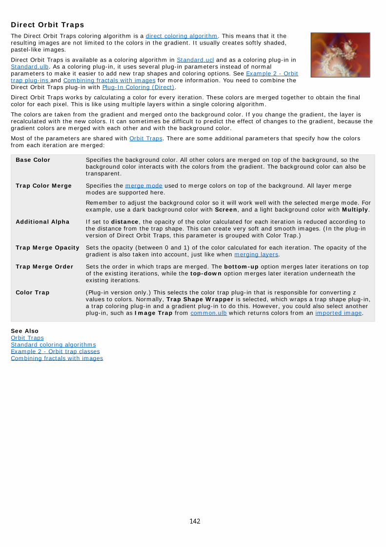
Direct Orbit TrapsThe Direct Orbit Traps coloring algorithm is a direct coloring algorithm. This means that it theresulting images are not limited to the colors in the gradient. It usually creates softly shaded,pastel-like images.

Direct Orbit Traps is available as a coloring algorithm in Standard.ucl and as a coloring plug-in inStandard.ulb. As a coloring plug-in, it uses several plug-in parameters instead of normalparameters to make it easier to add new trap shapes and coloring options. See Example 2 - Orbittrap plug-ins and Combining fractals with images for more information. You need to combine theDirect Orbit Traps plug-in with Plug-In Coloring (Direct).

Direct Orbit Traps works by calculating a color for every iteration. These colors are merged together to obtain the finalcolor for each pixel. This is like using multiple layers within a single coloring algorithm.

The colors are taken from the gradient and merged onto the background color. If you change the gradient, the layer isrecalculated with the new colors. It can sometimes be difficult to predict the effect of changes to the gradient, because thegradient colors are merged with each other and with the background color.

Most of the parameters are shared with Orbit Traps. There are some additional parameters that specify how the colorsfrom each iteration are merged:

Base Color Specifies the background color. All other colors are merged on top of the background, so thebackground color interacts with the colors from the gradient. The background color can also betransparent.

Trap Color Merge Specifies the merge mode used to merge colors on top of the background. All layer mergemodes are supported here.

Remember to adjust the background color so it will work well with the selected merge mode. Forexample, use a dark background color with Screen, and a light background color with Multiply.

Additional Alpha If set to distance, the opacity of the color calculated for each iteration is reduced according tothe distance from the trap shape. This can create very soft and smooth images. (In the plug-inversion of Direct Orbit Traps, this parameter is grouped with Color Trap.)

Trap Merge Opacity Sets the opacity (between 0 and 1) of the color calculated for each iteration. The opacity of thegradient is also taken into account, just like when merging layers.

Trap Merge Order Sets the order in which traps are merged. The bottom-up option merges later iterations on topof the existing iterations, while the top-down option merges later iteration underneath theexisting iterations.

Color Trap (Plug-in version only.) This selects the color trap plug-in that is responsible for converting zvalues to colors. Normally, Trap Shape Wrapper is selected, which wraps a trap shape plug-in,a trap coloring plug-in and a gradient plug-in to do this. However, you could also select anotherplug-in, such as Image Trap from common.ulb which returns colors from an imported image.

See AlsoOrbit TrapsStandard coloring algorithmsExample 2 - Orbit trap classesCombining fractals with images

Distance EstimatorThe Distance Estimator coloring algorithm estimates the distance between a pixel and the boundaryof the fractal (for example the boundary of the Mandelbrot set). The pixel is colored accordingly.

This coloring algorithm is especially good at showing the thin connecting lines and miniatures thatexist everywhere in the Mandelbrot set. It works correctly for divergent fractal formulas likeMandelbrot, Julia, and Phoenix.

The Exponent parameter should be set to match the exponent or power of the fractal formula (thisis usually also a parameter). Higher values (like 128) for the bail-out parameter of the fractalformula give the best results.

Distance Estimator is available as a coloring algorithm in Standard.ucl and as a coloring plug-in in Standard.ulb.

See AlsoBasicDecompositionStandard coloring algorithms

EmbossThe Emboss coloring algorithm interprets results from one of the Embossed fractal formulas tocreate fractals with 3D contour lines. It is unlikely to give good results with other fractal formulas.

See Embossed (Julia, Mandelbrot, Newton) for more information.

Emboss is available as a coloring algorithm in Standard.ucl and as a coloring plug-in inStandard.ulb.

See AlsoLightingStandard coloring algorithms

Exponential SmoothingThe Exponential Smoothing coloring algorithm creates smoothly colored outside areas. It workswell for both convergent and divergent fractal types, which means that it can be combined withalmost any fractal formula.

Fractal formulas like Mandelbrot, Julia, and Phoenix have only divergent orbits, while types likeNewton and Nova have only convergent orbits. The Magnet fractal formulas have both divergentand convergent orbits.

With the Color Divergent and Color Convergent parameters, you can enable coloring fordivergent and convergent orbits. You should always enable at least one option. The formula runs slightly faster if you justenable the necessary options (only Magnet-like fractals require both parameters to be enabled).

The Divergent Density parameter can be used to tweak the color density for divergent parts of a fractal. It is only usefulwhen both divergent and convergent orbits exist in the fractal.

Exponential Smoothing is available as a coloring algorithm in Standard.ucl and as a coloring plug-in in Standard.ulb.

See AlsoSmooth (Mandelbrot)Standard coloring algorithms

Gaussian IntegerThe Gaussian Integer coloring algorithm colors fractals according to how the calculated orbits arerelated to Gaussian integers.

Gaussian Integer is available as a coloring algorithm in Standard.ucl, or as a trap shape plug-in inStandard.ulb that can be used together with the Orbit Traps or Direct Orbit Traps coloring plug-ins.See Example 2 - Orbit trap plug-ins .

Gaussian integers are complex numbers normalized to integer values. This coloring algorithmexamines the values of z calculated by the fractal formula, and tests them against nearby Gaussianintegers.

The resulting images are richly textured, containing many circles, dots, and stars. By tweaking the provided parameters,many variations are possible.

The following parameters are available:

Integer Type Specifies the rounding method to use to find the nearest Gaussian integer. The round(z) optionusually gives smoother images than the other options.

Color By Selects how the color of each pixel is determined. For example, it can be colored by theminimum distance from a value of z to the nearest Gaussian integer.

Normalization Chooses between several ways of normalizing the distance to the nearest Gaussian integer. Ifyou select factor or f(z), an additional parameter will appear that specifies the normalizationfactor or function to use.

Randomize If checked, a small randomization factor is added to each value of z before examining itsbehavior. Additional parameters will appear to specify the amount of randomization and a seedvalue. Each seed value will give different randomization patterns.

In the trap shape plug-in version, this option is not available. However, you can achieve thesame effect by selecting the Randomize transformation plug-in from Standard.ulb for the TrapPosition parameter in the Orbit Traps plug-in.

See AlsoExample 2 - Orbit trap plug-ins Orbit TrapsStandard coloring algorithms

GradientThe Gradient coloring algorithm ignores the information from the fractal formula and fills the fractalwith all colors from the gradient.

To obtain a completely filled image, select the Gradient coloring algorithm in both the Inside andthe Outside tabs of the Layer Properties tool window. This ensures that all pixels are colored in thesame way.

The Gradient Type parameter selects how the gradient should be displayed: linear (from left toright), radially, or as a cone. Use zooming and panning to reposition the gradient as desired.

This coloring algorithm is handy for creating special effects with multi-layer images. You can, for example, use it in a masktogether with a suitable transparent gradient to show only selected portions in a regular pattern of the layer that ismasked.

Gradient is available as a coloring algorithm in Standard.ucl and as a coloring plug-in in Standard.ulb.

See AlsoStandard coloring algorithms

ImageThe Image coloring algorithm enables you to load an external image into a fractal. It simplydisplays the image in the inside or outside area of the fractal. If you want the entire layer to showthe image, the Image coloring algorithm is best combined with the standard Pixel fractal formula.

The Image parameter contains the image that is displayed. See Using images for more informationon how to use this parameter.

In the layer, the image is scaled such that it occupies the entire layer if the default location is set.To achieve this, load the Pixel fractal formula and click the Reset Location button on the Locationtab. Of course, you can pan, zoom, and rotate at will to frame or distort the image.

When zooming in, the individual pixels in the image are interpolated using sophisticated bicubic interpolation methods. Forthe best results when zooming out, it is recommended to render the fractal with anti-aliasing enabled.

Image is available as a coloring algorithm in Standard.ucl and as a coloring plug-in in Standard.ulb.

See AlsoStandard coloring algorithmsUsing images

LightingThe Lighting coloring algorithm interprets results from one of the Slope fractal formulas to createfractals with 3D lighting effects. It will probably not give very good results with other fractalformulas.

See Slope (Julia, Mandelbrot, Newton) for more information.

Lighting is available as a coloring algorithm in Standard.ucl and as a coloring plug-in inStandard.ulb.

See AlsoEmbossStandard coloring algorithms

NoneThe None coloring algorithm is the simplest coloring algorithm available. It is loaded by default inUltra Fractal when a new fractal is created.

None reproduces the standard iterations coloring algorithm found in most fractal software.

None is available as a coloring algorithm in Standard.ucl and as a coloring plug-in (called Default)in Standard.ulb.

See AlsoBasicStandard coloring algorithms

Orbit TrapsThe Orbit Traps coloring algorithm is an extremely versatile general-purpose coloring algorithm. Itcan be applied to almost any fractal formula with good results, on both the Inside and Outside tabs.

Orbit Traps is available as a coloring algorithm in Standard.ucl and as a coloring plug-in inStandard.ulb. As a coloring plug-in, it uses several plug-in parameters instead of normalparameters to make it easier to add new trap shapes and coloring options. You need to combinethe Orbit Traps plug-in with Plug-In Coloring (Gradient). See Example 2 - Orbit trap plug-ins for anexample of how this works in practice.

Orbit Traps works by examining the value of z (as calculated by the fractal formula) for each iteration. It tests how close zis to a fixed shape (the orbit trap), and colors the pixel according to the closest distance, for example.

The possibilities are almost unlimited because there are so many combinations of parameters available. It is a good idea totake some time to explore the different options in here.

The following parameters are available:

Trap Position (Plug-in version only.) Provides options to transform the value of z before it is passed to the trapshape plug-in. This essentially transforms the trap shape. The default Trap Position plug-in providesmany common options, but it is also possible to select any other transformation plug-in, or even tomerge multiple transformations with Transform Merge in common.ulb.

Trap Shape Specifies the shape of the orbit trap. Some options may not look too exciting with the default settingsof the other parameters, but try changing Trap Coloring and Trap Mode in that case. Not all optionswork equally well with all fractal types.

In the plug-in version, Trap Shape is a plug-in parameter that accepts any trap shape plug-in. All trapshapes from the Orbit Traps coloring algorithms are available as trap shape plug-ins in Standard.ulb.

Some trap shapes have additional parameters:

Diameter Specifies the diameter or size of the trap. Larger values usually create decorations further away fromthe center of the fractal.

Order Specifies the order for the trap, such as the number of leaves for the pinch trap shape. It depends onthe trap shape how this is interpreted. Larger values usually give more complex traps.

Frequency Specifies the frequency of ripples or waves (where applicable). Larger values create "busier" trapshapes with more frills.

Trap Transfer (Plug-in version only.) Provides options to transform the distance that is returned by the trap shapeplug-in. The default Trap Transfer plug-in is quite powerful, but it is also possible to select anothertransfer plug-in.

Trap Mode Selects how the values gathered at each iteration are interpreted to produce a color. For example, themagnitude at the closest distance to the trap shape is used if Trap Coloring is set to magnitude, andTrap Mode to closest.

Experiment to see which combinations work well together. Some trap modes only work well withspecific trap coloring settings, for example.

The trap only option will show the trap shape only. This is useful for learning how the other optionswork.

In the plug-in version, Trap Mode is a plug-in parameter that accepts any trap mode plug-in, and theoriginal trap mode options are now also available as trap mode plug-ins in Standard.ulb.

Trap Threshold Specifies the width of the trap area, used for most trap modes. (In the non-plug-in version, thisparameter is called Threshold.)

Trap Coloring The Trap Coloring parameter selects what information is gathered at each iteration. This is laterfiltered and combined to produce the final color.

In the plug-in version, Trap Coloring is a plug-in parameter that accepts any trap coloring plug-in,and the original trap coloring options are now also available as trap coloring plug-ins in Standard.ulb.

Use Solid Color If checked, areas outside the trap shape will be colored with the solid color (allowing them to betransparent).

The non-plug-in version of Orbit Traps does not have the Trap Position plug-in parameter that allows any transformation totransform the trap shape, but it does offer some transformation options:

Trap Center Specifies the center of the trap shape. Values other than (0, 0) will distort the trap shape into thedirection of the trap center. Use the eyedropper to select good values for this parameter.

Aspect Ratio Changes the aspect ratio of the trap shape. Values larger than 1 will stretch the trap horizontally;values smaller than 1 will stretch it vertically.

Rotation Rotates the trap shape in clockwise direction (specified in degrees).

See AlsoTutorial: MaskingExample 2 - Orbit traps plug-ins Direct Orbit TrapsStandard coloring algorithms

Plug-In Coloring (Gradient, Direct)Plug-In Coloring is a skeleton coloring algorithm that lets a coloring plug-in do the actual work. Allcoloring algorithms in Standard.ucl are also implemented as coloring plug-ins. You can select any ofthese as the coloring plug-in to be used together with Plug-In Coloring.

There are two versions of Plug-In Coloring: a gradient version and a direct version. Plug-In Coloring(Gradient) is a normal coloring algorithm and works only with gradient coloring plug-ins whichreturn an index into the gradient.

Plug-In Coloring (Direct) is a direct coloring algorithm and works with coloring plug-ins that directlyreturn a color. It also works with gradient coloring plug-ins, but in that case changes to the gradient trigger anunnecessary recalculation.

The Coloring Algorithm parameter sets the coloring plug-in to be used. By default, the Smooth (Mandelbrot) plug-infrom Standard.ulb is selected for Plug-In Coloring (Gradient), while Plug-In Coloring (Direct) defaults to the Direct OrbitTraps plug-in.

An example of using Plug-In Coloring is given in Example 2 - Orbit trap plug-ins.

See AlsoPlug-ins Standard coloring algorithms Standard plug-ins

Smooth (Mandelbrot)The Smooth (Mandelbrot) coloring algorithm creates smoothly colored outside regions with fractalformulas such as Mandelbrot and Julia.

It works with most divergent fractal formulas. For Newton and Nova fractals, use ExponentialSmoothing instead.

There are two parameters available: Exponent and Bail-out value. These should be set to matchthe corresponding parameters of the fractal formula. Otherwise, the coloring will not be perfectlysmooth.

Usually, the best results are obtained when the Transfer Function in the Outside tab is set to Log.

Smooth (Mandelbrot) is available as a coloring algorithm in Standard.ucl and as a coloring plug-in in Standard.ulb.

See AlsoBasicStandard coloring algorithms

Triangle Inequality AverageThe Triangle Inequality Average coloring algorithm creates smoothly colored fractals with largeflame-like patterns that extend from the fractal outwards.

Because it uses the same smoothing as Smooth (Mandelbrot), it only works with most divergentfractal formulas, such as Mandelbrot and Julia.

There are two parameters available: Exponent and Bailout. These should be set to match thecorresponding parameters of the fractal formula. Otherwise, the coloring will not be smooth.

Use very large bail-out values for good results. The default value 1e20 (a 1 with 20 zeroes) is a good starting point. TheMandelbrot (Built-in) formula cannot handle such large values, so use the non-built-in Mandelbrot instead.

Triangle Inequality Average is available as a coloring algorithm in Standard.ucl and as a coloring plug-in in Standard.ulb.

See AlsoOrbit TrapsStandard coloring algorithms

Transformations

Note: You need Ultra Fractal Creative Edition or Extended Edition to use transformations.

Transformations globally transform and warp the shape of a fractal. You can combine various transformations to createcomplex effects. Of course, you can also write your own transformations.

Transformations are managed in the Mapping tab of the Layer Properties tool window:

The Add button opens a modal browser to select a new transformation. The transformation is then added to the list.

The Delete button removes the selected transformations from the list.

The Reload button reloads the selected transformation from disk and recalculates the layer.

The Edit button opens the selected transformation in the formula editor.

The More button shows a menu with additional commands.

The Enable icon before a transformation quickly enables and disables the transformation.

The Solid Color swatch specifies the solid color for the selected transformations. The solid color can be used by atransformation for special purposes. See Solid color.

The transformation parameters are additional parameters specific to the selected transformations. See Formulaparameters.

You can resize the transformations list by dragging the area just above the line that divides the Solid Color setting fromthe transformation parameters. The Reload and Edit buttons hide themselves automatically when there is not enoughspace. In this case, these commands can be found on the More menu.

Next: Working with transformations

See AlsoTutorial: Learning about transformationsStandard transformationsFractal formulasColoring algorithms

Working with transformationsYou work with transformations in the Mapping tab of the Layer Properties tool window. The Mapping tab shows a list withthe transformations used by the active layer.

Transformations are stored in transformation files (*.uxf). Each file can contain multiple transformations.

To add a transformation, click the Add button. This opens a modal browser that shows the transformation files onyour computer and the transformations that they contain. Double-click on a transformation to add it.

Hold down the Add button to open a menu with transformation presets, together with a Recent menu that providesquick access to recently used transformations.

To remove the selected transformations, click the Delete button.

To rename the active transformation, click it again or press F2 (like in Windows Explorer).

To change the order in which transformations appear in the list, drag them up or down. See Multipletransformations.

The Enable icon before each transformation enables and disables it. Use it to temporarily disable a transformationso you can judge its effect, or adjust other transformations.

Some transformations contain additional help. To access it, click the More button, and then click Help from themenu that opens. This menu also provided commands to copy and paste the settings and parameters for theselected transformation, and to reset all parameters to the default values.

The bottom pane of the Mapping tab contains parameters specific to the selected transformations. These parameters workthe same as the parameters for fractal formulas. See Formula parameters.

Notes

You can select multiple transformations by holding down the Ctrl key while clicking a transformation. Hold down theShift key while clicking to select a range of transformations. This enables you to easily edit multiple transformationstogether, like you can do with layers.

If multiple layers are selected, the list in the Mapping tab only shows those transformations that all selected layershave in common.

Right-click inside the list of transformations to open a menu with frequently used commands.

Next: Multiple transformations

See AlsoTutorial: Learning about transformationsTransformationsStandard transformationsPublic formulas

Multiple transformationsUltra Fractal lets you combine multiple transformations to achieve more complex effects. With more than onetransformation, the order in which the transformations appear in the list in the Mapping tab of the Layer Properties toolwindow is important.

You can view a transformation as if it transforms the image of the layer as produced by the fractal formula and thecoloring algorithms. (In fact, it works differently, but you can ignore that unless you are writing your owntransformations.)

The transformations are then processed from the bottom of the list to the top. So, if you have two transformations, the topone works on the "image" produced by the second transformation.

Here is an example to illustrate this:

Original Inverse Lake

Two variations on the original image are shown. The first uses the Inverse transformation that turns an image "inside out".The second variation uses the Lake transformation that mirrors the image horizontally and creates the illusion of waterripples.

What happens if we combine the two transformations?

First Lake, then Inverse First Inverse, then Lake

If we put Inverse above Lake, we get the first image. If we put Lake on top instead, the second image is produced. Thisshows that a transformation works on the intermediate result produced by the transformations below it.

Notes

You can freely experiment with the order of the transformations by dragging them up or down in the list.

When you add a new transformation, it is always inserted above the selected transformation, so it works on theintermediate image produced by that transformation.

Next: Solid color

See AlsoTransformationsWorking with transformations

Solid colorIn the Mapping tab of the Layer Properties tool window, you can specify a solid color for each transformation. Atransformation can use this color for special purposes.

For example, a transformation that maps a fractal onto a plane in 3D space also needs to color the area that is above orbelow the plane. This area is usually colored with the solid color.

This example shows a simple fractal mapped onto a sphere with the 3D Mapping transformation. The area outside thesphere is given the solid color (in this case black).

To change the solid color, click on the Solid Color swatch in the Mapping tab. By default, it is set to black, but you canchoose any color. You can also change the opacity. By setting the opacity to 0, the solid color and thus the solid areas willbecome transparent, so the lower layers will become visible.

In effect, the transformation not only transforms the shape of the fractal, but also generates a mask for the layer.

Some transformations are only intended to create masks, and do not transform the pixels at all. You should use them witha transparent solid color. An example is the Clipping transformation.

Notes

If you make a solid color transparent, layer transparency will be enabled automatically. See Transparent layers.

The masks created with transformations always have sharp edges. For soft masking with more control over themasking shapes, use layer masks instead. See Masks.

Next: Standard transformations

See AlsoTransformationsWorking with transformations

Standard transformationsUltra Fractal comes with a set of standard transformations. They are located in the file Standard.uxf in the Formulas folder.It contains the following transformations:

3D Mapping

Aspect Ratio

Clipping

Glass Hemisphere

Inverse

Kaleidoscope

Lake

Mirror

Plug-In Clipping

Plug-In Transformation

Ripples

Twist

All standard transformations are also implemented as transformation or clip shape plug-ins in Standard.ulb. This makes itpossible to use them with Plug-In Transformation or Plug-In Clipping, or in other formulas that accept transformation plug-ins. See About plug-ins for more information.

See AlsoStandard fractal formulasStandard coloring algorithmsStandard plug-ins TransformationsPublic formulas

3D MappingThe 3D Mapping transformation maps a fractal onto a three-dimensional shape, such as a plane ora sphere. It is available as a transformation in Standard.uxf and as a transformation plug-in inStandard.ulb.

Once this transformation is in effect, normal zooming and panning will just move the 3D shapearound with the fractal on it. If you want to zoom into the fractal as it is mapped onto the shape,use the Fractal Center, Fractal Magnification, and Fractal Rotation parameters.

To use the rotation and translation parameters effectively, you need to understand the left-handed3D coordinate system used by the transformation. Here, the X-axis points to the left, the Y-axis points upwards, and theZ-axis points into the screen. So, if you use a positive Z-translation, the 3D shape will appear to move away, into thescreen.

The following parameters are available:

Shape Selects the type of 3D shape that the fractal is mapped onto. In the plug-in version of 3DMapping, this is a plug-in parameter that lets you select any plug-in that implements amapping shape.

X RotationY RotationZ Rotation

Rotates the 3D shape around the X, Y, or Z axis. To predict the direction of rotation, hold upyour left hand with your thumb pointing into the positive axis direction (for example, to the leftfor X rotation). Your (curled) fingers now show the direction of positive rotation around thataxis.

X TranslationY TranslationZ Translation

Moves the shape around in 3D space. You always need some positive Z translation to move theshape "into" the screen, otherwise you will be "inside" the shape and it won't be visible. Withthe plane shape, use a negative Y translation to look down upon it.

Fractal CenterFractal MagnificationFractal Rotation

Specifies the location of the fractal as it is mapped onto the shape. When adding thetransformation, the current coordinates will be used (remember to reset the location to get aproper view of the 3D shape).

The easiest way to specify a location is to copy the coordinates from the Location tab of adifferent fractal window that contains the same fractal formula without the 3D Mappingtransformation.

See AlsoTutorial: Learning about transformationsStandard transformations

Aspect RatioThe Aspect Ratio transformation can be used to create fractals for media with non-square pixels.You should add it to all layers of the fractal. It is available as a transformation in Standard.uxf andas a transformation plug-in in Standard.ulb.

The Aspect Ratio parameter specifies the aspect ratio (height / width) of the final media. The finalmedia is the computer screen or printed poster that will eventually display the fractal. If the valueof the parameter is equal to the height divided by the width of the fractal window, no stretchingoccurs.

For example, suppose you would like to display a fractal on a 15" x 10" screen that has a resolution of 400 x 300 pixels.Here, the pixels are wider than tall. You would set the width and height of the fractal window to 400 x 300 to obtain thedesired size. Then, set the Aspect Ratio parameter of this transformation to 0.6667 (10" / 15").

Most computer monitors and printers have square pixels. In this case, you do not need to use this transformation. If youjust want to stretch the fractal, use the Stretch parameter in the Location tab of the Layer Properties tool window instead.

See AlsoStandard transformations

ClippingThe Clipping transformation cuts a geometric shape out of a fractal. The shape is filled with a solidcolor. It can also be transparent, to make parts of the underlying layers visible.

Clipping is available as a transformation in Standard.uxf and as a clip shape plug-in inStandard.ulb. In plug-in form, it can be used together with Plug-In Clipping. In this case, it alsoshows handles in the fractal window to show where the edges of the clipping shape are.

Both rectangular and circular shapes are available. You can choose to cut either the region inside oroutside the shape. This makes the Clipping transformation also useful for creating frames.

The following parameters are available:

Center Specifies the coordinates of the center of the clipping shape. Use the eyedropper (right-click andclick Eyedropper) to select the center by clicking inside the fractal window.

Right Edge Specifies the coordinates of the right edge of the clipping shape. Use the eyedropper to select this.

Top Edge Specifies the coordinates of the top edge of the clipping shape. Use the eyedropper to select this.

Shape Selects the type of shape to use. If you select circle or square, the Top Edge parameter is ignored.

Allow Rotation If checked, the shape is allowed to rotate. In this case, the Right Edge parameter also defines therotation to use.

Region Selects whether to cut the region outside the clipping shape, or inside the clipping shape. (Thisparameter is not available in the Clipping plug-in.)

Screen-Relative If checked, all coordinates are interpreted as relative to the screen. This makes it harder to entercoordinates (because you can no longer use the eyedropper), but it preserves the location of theclipping shape relative to the screen when zooming. (This parameter is not available in the Clippingplug-in.)

See AlsoTutorial: Learning about transformationsStandard transformations

Glass HemisphereThe Glass Hemisphere transformation displays the fractal as though it is viewed through a sphericallens. It is available as a transformation in Standard.uxf and as a transformation plug-in inStandard.ulb.

The location, size, and apparent refractive index of the lens can be changed. The refractive indexadjusts the strength of the lens.

The following parameters are available:

Refractive index Specifies the refractive index of the lens. You can use this to simulate various glass-like materials.Larger values will increase the strength of the lens.

Width Specifies the width of the lens in fractal coordinates.

Center Specifies the coordinates of the center of the lens. Use the eyedropper (right-click and clickEyedropper) to select the center by clicking inside the fractal window.

Use Screen Center If checked, the center of the screen is used instead of the Center parameter, so the lens is alwayscentered on the screen, even when zooming in.

See AlsoStandard transformations

InverseThe Inverse transformation turns a fractal inside out. The original center of the fractal is putinfinitely far away, and points that were far away end up near the center. Inverse is available as atransformation in Standard.uxf and as a transformation plug-in in Standard.ulb.

This can change the shape of the fractal in unexpected ways. The example image shows theInverse transformation applied to a standard Mandelbrot set. (The inside areas of the Mandelbrotset are colored gray.)

The following parameters are available:

Radius Specifies the radius of the inversion circle. The transformation inverts all points around this circle.Larger values will simply magnify the inverted fractal.

Center Specifies the coordinates of the center of the inversion circle. This will drastically change the shapeand form of the fractal. Use the eyedropper (right-click and click Eyedropper) to select the centerby clicking inside the fractal window.

Use Screen Center If checked, the center of the screen is used instead of the Center parameter, so the inversioncircle is always centered on the screen. This can give unexpected effects when zooming in.

See AlsoStandard transformations

KaleidoscopeThe Kaleidoscope transformation fills the screen with rotated copies of a small radial slice of thefractal, creating a kaleidoscope effect. It is available as a transformation in Standard.uxf and as atransformation plug-in in Standard.ulb.

By tweaking the parameters, you can simulate many different kinds of symmetry. By default, theslices are aligned and mirrored to make the edges match, but there are also other options thatproduce sharp transitions.

Try experimenting with the Center and Rotation angle parameters to obtain good results. Somesections of the fractal lend themselves much better to the kaleidoscope effect than others.

The following parameters are available:

Symmetry Order Sets the symmetry order. This is the number of times the slice of the fractal is copied and rotatedto obtain the final image.

Symmetry Mode Selects the symmetry mode to use. Only the reflective option is guaranteed to produce seamlessimages. Use the slice only option to view the slice of the fractal that is used as a base for thesymmetry effect.

Center Specifies the coordinates of the symmetry center. Together with the Rotation angle parameter,this selects the slice of the fractal that is used. Try changing this to see the various effects that arepossible.

Use the eyedropper (right-click and click Eyedropper) to select the center by clicking inside thefractal window.

Use Screen Center If checked, the center of the screen is used instead of the Center parameter, so the symmetrycenter is always centered on the screen. This can give unexpected effects when zooming in.

Rotation angle Rotates the fractal before determining the slice that will be used as a base for the symmetryeffect. This can drastically change the resulting image.

See AlsoMirrorStandard transformations

LakeThe Lake transformation mirrors the fractal in a rippled lake. The top part of the fractal is notaltered, but below the water level, everything is mirrored. It is available as a transformation inStandard.uxf and as a transformation plug-in in Standard.ulb.

By changing the parameters, you can adjust the height and rotation of the water level, and changethe size and frequency of the waves.

The following parameters are available:

Water level Selects the water level. Only the imaginary part of this parameter is used. Use theeyedropper (right-click and click Eyedropper) to select the water level by clicking on a pointinside the fractal window.

Use screen center If checked, the water level is always centered on the screen. In this case, the Water levelparameter is ignored.

Rotation angle Rotates the water level. To rotate the fractal instead of the water, also enter the same valuein the Rotation angle parameter on the Location tab.

Use Location tab angle If checked, the rotation angle from the Location tab is used instead of the Rotation angleparameter. This ensures that the water level is always horizontal.

Amplitude Specifies the amplitude of the waves.

Frequency Specifies the frequency of the waves.

See AlsoRipplesStandard transformations

MirrorThe Mirror transformation mirrors the fractal along an arbitrary axis. It can be useful for mirroringeffects with multiple layers. It is available as a transformation in Standard.uxf and as atransformation plug-in in Standard.ulb.

There are presets for a horizontal and a vertical reflection axis, but you can also specify any angle.The center of the axis is configurable, too.

The following parameters are available:

Reflection Axis Selects the reflection axis. The axis points into the mirroring direction, so it is perpendicular tothe imaginary mirror. Select arbitrary to specify any angle for the axis.

Reflection Angle Specifies the rotation angle of the reflection axis, in degrees.

Center Selects the center of the reflection axis. Use the eyedropper (right-click and click Eyedropper) toselect a point by inside the fractal window.

Use screen center If checked, the reflection center is always centered on the screen. In this case, the Centerparameter is ignored.

See AlsoKaleidoscopeStandard transformations

Plug-In ClippingThe Plug-In Clipping transformation cuts a shape out of a fractal. The shape is determined by a clipshape plug-in, and Plug-In Clipping allows any compatible clip shape plug-in to be selected.

By default, the Clipping plug-in from Standard.ulb is selected.

The following parameters are available:

Clipping Region Selects whether to cut the region outside the clipping shape, or inside the clipping shape.

Screen-RelativeCoordinates

If checked, all coordinates are interpreted as relative to the screen. This makes it harder to entercoordinates (because you can no longer use the eyedropper), but it preserves the location of theclipping shape relative to the screen when zooming. The coordinates are interpreted with (0, 0) atthe lower left corner of the fractal window and (1, 1) at the upper right corner.

Clipping Shape This is the clip shape plug-in parameter. You can select any plug-in that represents a clippingshape.

Plug-In Clipping can also show handles around the edges of a clipping shape. The number and position of these handlesare determined by the selected clipping shape. By default, handles are shown in the fractal window, but not whenrendering or on previews. Under Handle options, this can be configured:

Show Handles Sets whether handles are displayed at all.

Not on previews If checked, handles are hidden on previews, for example in the browser or for explore oreyedropper previews.

Not on renders If checked, handles are hidden when rendering to disk.Show Numbers If checked, a number or label is displayed next to each handle if applicable.Show Lines If checked, lines are displayed if applicable.Handle Size Adjusts the apparent size of the handles.Handle Thickness Adjusts the apparent thickness of the handles.

Note: Handles are shown by toggling the solid color of the transformation on and off, so you might not see them properlyif the solid color does not contrast with the fractal. Also, they do not work well in combination with the Guessing drawingmethod.

See AlsoPlug-ins Standard transformationsStandard plug-ins

Plug-In TransformationPlug-In Transformation is a skeleton transformation that lets a transformation plug-in do the actualwork. All transformations in Standard.uxf are also implemented as transformation plug-ins. You canselect any of these as the transformation plug-in to be used together with Plug-In Transformation.

The Transformation parameter sets the transformation plug-in to be used. By default, the Inverseplug-in from Standard.ulb is selected.

See AlsoPlug-ins Standard transformationsStandard plug-ins

RipplesThe Ripples transformation adds a water ripple effect to the fractal. The center, strength, andfrequency of the ripples are adjustable. It is available as a transformation in Standard.uxf and as atransformation plug-in in Standard.ulb.

Interesting interference effects are obtained by adding multiple Ripple transformations to a fractal,with different center and strength values.

The following parameters are available:

Ripple Center Specifies the center of ripples. Use the eyedropper (right-click and click Eyedropper) to selectthis by clicking on a point inside the fractal window.

Use Screen Center If checked, the ripple center is always centered on the screen. In this case, the Ripple Centerparameter is ignored.

Ripple Strength Specifies the strength of the ripples. Larger values give a larger distortion.

Ripple Frequency Specifies the frequency of the ripples. Larger values will create more and smaller ripples.

Ripple Fade Specifies how soon the ripples fade out. Larger values cause the ripples to fade out over a largerdistance (so more ripples are visible).

Ripple Type Selects how the ripples distort the fractal. The default Forward and Back option gives the mostnatural water-like effect, but the other options are also interesting.

See AlsoLakeTwistStandard transformations

TwistThe Twist transformation adds a twisted spiral to the fractal. It distorts a small part of the fractal inthe form of a spiral, like a vortex. It is available as a transformation in Standard.uxf and as atransformation plug-in in Standard.ulb.

The center, strength, and size of the vortex are adjustable. This transformation is often combinedwith the Ripples transformation to obtain interference effects.

The following parameters are available:

Twist Center Specifies the center of the twisted spiral. Use the eyedropper (right-click and click Eyedropper)to select this by clicking on a point inside the fractal window.

Strength Specifies the strength of the twist. Larger values create more strongly twisted spirals.

Decay Factor Specifies how soon the spiral loses its strength. Larger values decrease the size of the spiral.

See AlsoLakeStandard transformations

Plug-insSince the first release of Ultra Fractal in 1998, the formulas written for it have become largerand more complex. Even though many formulas are quite similar, they could not share anycommon code, but had to be written as stand-alone formulas. For example, if you wanted toadd just one new feature to an existing formula written by someone else, you had to createa new formula, duplicate all the code from the original formula, and only then add some newthings.

To improve this situation, Ultra Fractal 5 introduced the ability for formulas to re-usecommon code via plug-ins. You can view a plug-in as a "black box" that adds functionalityto a formula. Via plug-in parameters, a formula enables you to select the actual plug-in thatperforms an action for the formula.

The formula declares what kind of functionality it needs and you can select any compatible plug-in to actually implement it.This makes it possible for formula authors to write a new plug-in to implement just the new feature that they want to addto an existing formula. The formula doesn't have to be changed at all. You just select the new plug-in when you use theformula.

For everyday users, plug-ins make it possible to combine existing elements in new ways without needing to do anyprogramming. For formula authors, plug-ins make it easier to write and manage complex formulas.

Next: Example 1 - Formula plug-ins

See AlsoFractal formulasWriting formulas

Example 1 - Formula plug-ins

Tip: This example assumes that you are familiar with Ultra Fractal basics as explained in the tutorials.

As a first example of how plug-ins work in practice, let's take a look at some of the standard plug-ins that come with UltraFractal.

First, use the browser to open the Default parameter set in Examples.upr. Click the Browse button in the Formula tab of the Layer Properties tool window to select Plug-In Formula in

Standard.ufm.

Plug-In Formula is a "skeleton" formula that lets a plug-in implement the actual fractal formula behavior. It has just oneplug-in parameter called Fractal Formula which is set to the Mandelbrot plug-in by default:

The Mandelbrot plug-in has its own parameters like Starting point, which appear grouped with the plug-in parameter. Let'sselect a different formula plug-in.

Click the Browse button for the Fractal Formula parameter to select a new plug-in. This opens the browser inplug-in mode, so it shows only those plug-ins that are compatible with this plug-in parameter.

Locate the Newton plug-in in Standard.ulb and click OK.

Now, a Newton fractal appears instead of a Mandelbrot fractal. Formula authors could make a formula plug-in that workswith Plug-In Formula to create a different fractal, without having to modify Plug-In Formula itself. Of course, this doesn'treally do anything new, since you could also just write a new fractal formula. But it does make the formula behavioravailable in a generic form.

Click the Browse button for the Fractal Formula parameter again, and this time, select the Slope plug-in.

Briefly go to the Outside tab of the Layer Properties and click the Browse button there to select the Lightingcoloring algorithm. Then go back to the Formula tab again.

The combination of the Slope formula plug-in and the Lighting coloring algorithm creates a 3D lighting effect. Previously,there were three different Slope formulas for Mandelbrot, Julia, and Newton fractals (these are still in Standard.ufm). Eachof these formulas duplicates the code for the lighting effect; the only different code is the where the actual fractal formulacalculation is done. Adding a new fractal type could only be done by creating yet another variation of this formula.

However, now the Slope formula plug-in contains another plug-in parameter that enables you to select the internal fractalformula. You can select any formula plug-in, just like with Plug-In Formula.

Click the Browse button for the Fractal Formula parameter inside the Slope plug-in (which currently is set toMandelbrot) and select Phoenix (Mandelbrot) instead.

Suddenly, we have a Slope formula that works with any fractal type. New fractal types can be added simply by writingthem as a formula plug-in, which makes them available for Plug-In Formula, Slope, or any other place where a fractalformula can be inserted.

Next: Example 2 - Orbit trap plug-ins

See AlsoPlug-insFractal formulasWriting formulas

Example 2 - Orbit trap plug-ins

Tip: This example assumes that you are familiar with Ultra Fractal basics as explained in the tutorials.

In the previous example, we saw how a formula plug-in can implement the behavior of an entire fractal formula. However,it's also possible to use plug-ins in a more fine-grained way, exposing all aspects of a formula for maximum flexibility.

The Orbit Traps coloring plug-in is an example of this. The old Orbit Traps coloring algorithm (still available inStandard.ucl) contained parameters such as trap shape, trap mode and trap coloring, each with a number of options. Inthe new version, implemented as a coloring plug-in in Standard.ulb, these are now plug-in parameters. Every major optionis now handled by a separate plug-in. Let's have a look:

First, use the browser to open the Default parameter set in Examples.upr. Click the Browse button in the Outside tab of the Layer Properties tool window to select Plug-In Coloring (Gradient)

in Standard.ucl.

Like Plug-In Formula, Plug-In Coloring (Gradient) is a skeleton coloring algorithm that lets a coloring plug-in do the work.By default, it loads with the Smooth algorithm.

Click the Browse button for the Coloring Algorithm parameter to select the Orbit Traps plug-in in Standard.ulb.

As you can see, the Orbit Traps plug-in uses plug-in parameters for all major parameters. All trap shapes, for example, arenow implemented as separate plug-ins. Let's select a different trap shape.

Click the Browse button for the Trap Shape parameter to select the Gaussian Integer plug-in.

The old Gaussian Integer coloring algorithm in Standard.ucl actually is a variation on an orbit trap, just with a differenttrap shape. It had limited options to color the trap shape, but now that it is available as a general trap shape plug-in, wecan combine it with any trap mode or trap coloring.

For example, you can select Angle to Origin 2 as the trap coloring to get an effect that you couldn't create with theoriginal Gaussian Integer coloring algorithm.

When formula authors write new trap shapes, trap modes or trap colorings and make them available in plug-in library filesvia the public formula library, you can just drop them into this standard Orbit Traps plug-in to use them.

Next: Working with plug-ins

See AlsoPlug-ins Coloring algorithms Writing formulas

Working with plug-insPlug-ins are commonly stored in plug-in library files with an .ulb extension. Like all formula files, you can examine andorganize plug-in library files with the browser. Make sure all files are visible, or set the file type to Plug-Ins.

Usually though, you'll work with plug-ins via plug-in parameters in the formula parameters list.

Click the Browse button for a plug-in parameter to select a different plug-in. A modal browser window opens,which shows only those plug-ins that are compatible with the current parameter.

Tip: In the browser window, click the Find Entries button and leave all fields blank to get a list of all compatibleplug-ins in the formula library.

Hold down the Browse button for a menu with other options:

Click Recent to open a menu with a list of recently used plug-ins, so you can quickly select one of these. Click Copy to copy the currently selected plug-in with all its sub-parameters to the Clipboard.

Click Paste to copy the plug-in information on the Clipboard to the plug-in parameter. The plug-in parameter mustbe compatible with the plug-in parameter that you copied the plug-in information from, otherwise an error messageis shown.

Click Reset Plug-In to select the default plug-in for the plug-in parameter. Click Reset Parameters to reset the sub-parameters for the currently selected plug-in to their default values. The

plug-in itself stays the same. Click Edit to open the class declaration for the plug-in in the formula editor.

Next: Standard plug-ins

See AlsoPlug-ins Working with formulasWriting formulas

Standard plug-insAll standard transformations, fractal formulas and coloring algorithms that come with Ultra Fractal are also available asplug-ins in the Standard.ulb file. This file is installed with the other standard formula files in the main formula folder. Formore information, see the documentation for the standard formulas:

Standard transformations

Standard fractal formulas

Standard coloring algorithms

For tips on how to use the standard plug-ins, see the plug-in usage examples.

Generally, to get as much formulas and plug-ins working together as possible, it is necessary for them to share thedefinition for common types of plug-ins. These shared definitions are in the file common.ulb. By adhering to thesedefinitions, different formulas and plug-ins from different formula authors can easily work with each other. Thecommon.ulb file is installed in the folder for public formulas so it can be updated automatically via the online formuladatabase when necessary.

The common.ulb file is intended mainly for formula authors. For everyday users, it does contain some useful plug-ins:

Clip Shape Merge allows a single clip shape parameter to accept multiple clip shapes. See Plug-In Clipping.

Image Trap allows an image to be used as a color trap for the Direct Orbit Traps coloring plug-in.

Transform Merge allows a single transformation parameter to accept multiple transformations. See Plug-InTransformation.

Trap Shape Block and Trap Shape Merge allows a single trap shape parameter to accept multiple trap shapes,and to transform trap shapes. See also Example 2 - Orbit trap plug-ins.

For formula authors, the common.ulb file is invaluable and almost any plug-in you write should be based on one of thebase classes found here. If you think modifications or new base classes are needed, please e-mail to info@ultrafractal.comor the UF programmers mailing list with your suggestion.

See AlsoAbout plug-ins Writing formulas

Layers

Note: You need Ultra Fractal Creative Edition or Extended Edition to use layers.

One of Ultra Fractal's key features is the ability to use multiple layers. Each layer contains a separate fractal image. Byusing multiple layers, you can achieve many special and wonderful effects that are not possible with single-layer images.

Layers are managed in the Layers tab of the Fractal Properties tool window:

The layers list shows all layers of the active fractal window, complete with previews. It also selects the active layer. Theactive layer is edited by the Layer Properties tool window and the gradient editor.

The Add button duplicates the active layer or group. Hold down the Add button to open a menu with more optionsand layer presets. See Presets.

The New Group button adds a new layer group to the layers list. See Layer groups.

The Delete button deletes the currently selected layers.

The Merge Mode input box selects the merge mode of the selected layers.

The Opacity slider changes the opacity of the selected layers.

The Visible, Editable and Transparent icons before each layer toggle the visibility, editability, and transparency ofthe layer. See Working with layers.

The Use as Mask button turns a layer into a mask and back. The Show Mask Only button makes it easier to edit amask. See Masks.

Next: How layers are merged

See AlsoTutorial: Working with layersKeyboard shortcuts for the Fractal Properties tool windowLayer groups Animating layers

How layers are mergedWithin a multi-layered fractal, Ultra Fractal merges the different layers to create the resulting image. This image appearsin the fractal window. The layers are merged by superimposing them.

Ultra Fractal starts with the bottom layer and places the second layer on top of it. The third layer (if any) is in turn placedon top of the result, and so on. If a layer is completely opaque, the layers below it will be hidden. If a layer is completelytransparent, it will not be visible.

Most layers will be more or less transparent, so they are visible while still allowing the lower layers to shine through. Thereare four ways to make layers transparent:

Reduce the opacity of the layer. By default, the opacity is set to 100%, making the layer fully opaque. Move theopacity slider to the left to make the active layer more transparent.

Change the merge mode of the layer. By default, the merge mode is set to Normal. The other merge modes createspecial effects that allow lower layers to be partially visible even if the opacity of the layer is set to 100%. See Mergemodes.

Make only parts of the layer transparent. The previous two options affect the entire layer. You can, however, alsochange the opacity of only certain areas in the layer. See Transparent layers.

Add a mask to the layer. The mask allows even more control over which areas of the layer will be transparent. SeeMasks.

Of course, you can freely mix these options. It is common, for example, to use a merge mode like Hard Light and set theopacity to less than 100%.

Next: Working with layers

See AlsoLayersTutorial: Working with layers

Working with layersLayers are managed in the Layers tab of the Fractal Properties tool window.

Click the Add button to add a new layer, duplicating the active layer.Hold down the Add button to open a menu with layer presets. See Presets.

Click the Delete button to delete the currently selected layers.

Click the New Group button to create a new layer group. See Layer groups.

Most commands and tool windows (such as the Layer Properties tool window) work on the currently selected layers. So, byselecting layers in the layers list, you change what is being edited by these other tool windows.

To select a layer, simply click it in the layers list.

To select multiple layers, hold down the Ctrl key and click the layers you want to add to the selection. Ctrl-click aselected layer to deselect it again.

To select a range of layers, click the first layer. Then, hold down the Shift key and click the last layer.

The Merge mode drop-down box selects the merge mode of the selected layers. The merge mode determines howthe layer is combined with the layers below it.

The Opacity slider adjusts the opacity of the selected layers. Move it to the left to make the layer less visible (moretransparent). Move it to the right to make it more opaque.

To rename the active layer, click it again or press F2 (like in Windows Explorer).

To move layers around in the list, drag the selected layers up or down. Of course, this affects the way the layers arecomposited.

To the left of each layer is a row of icons. These icons toggle various properties.

The Visible icon toggles the visibility of the layer. Use it to temporarily hide a layer, so you can more clearly seethe other layers.

The Editable icon selects whether a layer is editable. Only editable layers are affected by zooming operations. Bydefault, all layers are editable, so if you want to zoom in on only one layer, you should clear this icon on the otherlayers first.

The Transparent icon selects whether transparent areas in a layer are visible. See Transparent layers.

Notes

By holding down the Shift key while clicking on the Visible, Editable, or Transparent icons, you toggle all otherlayers instead. If you want to see just one layer, for example, Shift-click its Visible icon and all other layers will beturned off. Shift-click it again to show all layers.

If a layer is not editable, its properties can still be changed with the Layer Properties tool window. The Editable icononly affects zooming operations.

To copy the selected layers to another fractal window, drag them from the list of layers to the other fractal window.

Right-click in the list of layers to open a menu with frequently used commands. This menu also contains Copy andPaste commands that are another way of copying layers to other fractal windows.

Next: Merge modes

See AlsoTutorial: Working with layersWorking with masks Keyboard shortcuts for the Fractal Properties tool window Animating layers

Merge modesThe Merge mode drop-down box at the top of the Layers tab of the Fractal Properties tool window selects the mergemode of the selected layers. The merge mode defines how a layer is combined with the underlying layers to create thefinal image. The table below lists all merge modes and what they do.

The best way to learn how to use the different merge modes is to experiment. Also try to use various settings of theOpacity slider and see how it controls the intensity of the merging effects.

Next: Transparent layers

Merge mode Description

Pass Through This mode is only available for layer groups. The layers in the group will be merged as if they wereoutside the group.

Normal Directly returns colors from the layer. Use this if you don't want any special effects.

Multiply Multiplies the layer with the underlying layers. The result is always a darker color, thus darkening theunderlying layers.

Screen Multiplies the inverse of the layer with the inverse of the underlying layers, and inverts that again.The result is always a lighter color, thus brightening the underlying layers. Screen is the inverse ofMultiply.

Overlay Multiplies or screens the colors, depending on the color in the underlying layers. Creates colorblending effects between the layer and the underlying layers.

Hard Light Multiplies or screens the colors, depending on the color in the layer. Emphasizes the dark and lightregions in the layer, while the areas with medium brightness become transparent. Useful if the layercontains shadows or embossing effects.

Soft Light Darkens or lightens the colors, depending on the color in the layer. Creates an effect similar to HardLight, but with less emphasis on the dark and light areas in the layer.

Darken Returns the darkest of the color in the layer and the color in the underlying layers.

Lighten Returns the lightest of the color in the layer and the color in the underlying layers.

Difference Returns the difference between the layer and the underlying layers. Often creates unusual andunexpected color transitions.

Hue Returns the hue of the layer, and the saturation and luminance of the underlying layers. Colors theunderlying layers with the hue of the layer.

Saturation Returns the saturation of the layer, and the hue and luminance of the underlying layers. Changes thesaturation of the underlying layers depending on the layer.

Color Returns the hue and saturation of the layer, and the luminance of the underlying layers. Colors theunderlying layers with the layer. The underlying layers control the brightness of the resulting image.

Luminance Returns the luminance of the layer, and the hue and saturation of the underlying layers. The layercontrols the brightness of the underlying layers. Luminance is the inverse of Color.

Addition Directly adds the layer to the underlying layers, limiting the resulting colors at white (255, 255, 255).

Subtraction Directly subtracts the layer from the underlying layers, limiting the resulting colors at black (0, 0, 0).Difference is similar, but returns the absolute value after subtracting.

HSL Addition Adds the layer to the underlying layers using the HSL color model. Creates unusual effects.

Red Returns the red part of the layer, and the green and blue parts of the underlying layers.

Green Returns the green part of the layer, and the red and blue parts of the underlying layers.

Blue Returns the blue part of the layer, and the red and green parts of the underlying layers.

See AlsoHow layers are mergedLayers

Transparent layersTo make a layer transparent, you can use the Opacity and Merge mode settings, but these work on the entire layer. Youcan also make only certain parts of a layer transparent, which gives you more artistic control.

The easiest way to create transparent areas in a layer is to use a transparent gradient. The transparent parts of thegradient will create transparent areas in the layer. If you make all the other layers invisible, a pattern of blocks will showthe transparent areas.

Another way of creating transparent areas is to use the Solid Color setting of transformations and coloring algorithms.Solid colors with an opacity value of less than 255 create transparent areas. Many transformations, such as Clipping inStandard.uxf, use this to create masking effects.

The Transparent icon before the layer toggles transparent areas on and off. Use it to quickly verify the transparentareas and to see what difference they make to the final image.By default, transparency is off, but it is automatically turned on when you make changes to transparent areas in thelayer.

Next: Masks

See AlsoTutorial: Working with layersHow layers are mergedLayers

MasksIf you create transparent areas in a layer using a transparent gradient, the shape of the transparent areas is controlled bythe selected coloring algorithms. Certain colors in the gradient are transparent, so those colors will become transparent inthe layer, too. This means that you cannot use this method to create arbitrarily shaped transparent areas.

If you use transformations instead and set the opacity of the solid color to less than 255, you can create arbitrarily shapedtransparent areas in the layer. You do need a transformation that will output the area you need, but you could write ityourself. Still, a limitation of this technique is that pixels are either set to the solid color (transparent), or they are coloredaccording to the gradient and the selected coloring algorithms. You can only create sharp edges, not smooth transitions.

Masks overcome these problems. A mask is an invisible layer that is attached to the layer that needs transparent areas.The mask contains transparent areas, that are created with an ordinary transparent gradient. Since the mask is invisible,these transparent areas are invisible as well.

Instead, the layer owning the mask "borrows" the transparent areas of the mask. The shape of these areas is defined bythe selected fractal formula, the selected coloring algorithms, and the gradient of the mask. The shape is independentfrom the layer owning the mask.

Layer that needs transparent areas Mask with transparent areas Layer with the mask applied

As you can see, the layer uses the transparent areas of the mask. The colors in the mask layer are ignored.

Layers can have multiple masks to add differently shaped transparent areas. If the layer contains transparent areas itself(for example created with a transparent gradient), these are also taken into account.

Next: Working with masks

See AlsoTutorial: Masking Layers

Working with masksMasks are managed in the Layers tab of the Fractal Properties tool window.

To duplicate the active layer as a mask, hold down the Add button and click Duplicate as Mask in the menu thatappears.

To delete a mask, select it and click the Delete button.

To turn an existing layer into a mask, click the Use as Mask button. The layer will become a mask, attached to thelayer directly above it.

Click the Show Mask Only button to disable the layer owning the mask. Instead, the transparent areas in themask will be shown. White areas are opaque, black areas are transparent. This makes it easier to edit the mask.

Usually, the mask will be entirely white because its gradient is not yet transparent. The first thing to do is to open thegradient editor. Note that only the opacity view of the editor is enabled, since the colors in the gradient do not matter for amask. Add a few extra control points to the gradient so it will start to show some transparency (darker regions).

By toggling the Show Mask Only button, you can alternatively work on the mask and judge the effects that it has on thelayer that owns it. The mask can be edited like any layer. For example, you can zoom in on it, select another coloringalgorithm, and so on.

Notes

You can duplicate a mask layer like any other layer by clicking the Add button.

Layer groups can also have a mask. Just drag an existing mask layer onto the layer group, or position the layer touse as a mask just below the group (but not in it) and click the Use as Mask button.

Masks can be moved to other layers or layer groups simply by dragging them onto the desired layer or layer group.

A layer or layer group can have more than one mask. In this case, the transparent areas in the masks are combined,so each additional mask makes the layer more transparent.

Next: Layer groups

See AlsoTutorial: MaskingMasksWorking with layers Layers

Layer groupsYou can organize the layers in a fractal with layer groups. A layer group can contain any number of layers and nestedlayer groups. By logically arranging your layers in groups, the layers list becomes easier to manage. In addition, you canapply masks and merge modes to the entire group, which makes new creative effects possible.

Layer groups appear in the layers list with a folder-like group icon and a triangular collapse/expand button. Click thisbutton to hide or show the items in the group. Layers in a group appear below it, indented to show their relationship.

Click the New Group button to create a new layer group. The layer group starts empty. To fill the group, simplydrag one or more layer onto the group to move them inside. (Remember that you can Ctrl-click or Shift-click toselect multiple layers.)

To delete a layer group, select it and click the Delete button. This also deletes all items that the layer groupcontains. Tip: you can always undo unwanted deletions.

You can easily move layers in and out of groups by dragging them around. While you are dragging, a thick black lineshows where the dragged layers will end up. You can also nest groups simply by dragging one group inside another.Another way to move layers in and out of groups is with the Move Up and Move Down commands in the right-click menufor the layers list.

Layer groups have a merge mode just like layers, but with an additional Pass Through mode which is the default. If PassThrough is selected, the layers in the group are merged with the underlying layers one by one, as if they were not in agroup at all. With the Pass Through merge mode and Opacity at 100%, the layer group organizes its layers withoutintroducing any visual changes.

If a merge mode other than Pass Through is selected, the layers in the group are first merged together. Then, thatintermediate result is in turn merged onto the underlying layers with the merge mode for the layer group. The resultingeffect is often not possible to create without layer groups.

A group can also have a mask. In this case, the mask is applied to all layers in the group. Such a mask appears below allother items in the group, aligned with the group itself, as shown in the screen shot above. To turn a layer into a groupmask, position it just under the group (but not inside it), and click the Use as Mask button. To apply an existing mask toa group, simply drag it onto the group. See also Working with masks.

See AlsoLayersHow layers are merged Masks

Animation

Note: You need Ultra Fractal Extended Edition to work with animations.

Any fractal in Ultra Fractal can easily be turned into an animation. You can animate all parameters of the fractal at will andsee the result immediately in the fractal window. Finally, render the animation to watch it as a movie clip.

Creating and editing animations is done with various tools:

The animation bar contains the time slider and vital animation controls that enable you to create, edit, and playback animations. See Animation bar.

With the time slider, you set the current frame. The fractal window always displays the image for the currentframe.

The red animation indicators are shown if the fractal is currently in Animate mode. In Animate mode, changes thatyou make to the fractal are only applied to the current frame. If Animate mode is off (the default), your changes areapplied to the entire range of frames.

The key icons show at which frames and for which parameters keys have been recorded. See Animation keys.

The Timeline tool window provides an in-depth view of all animated settings and parameters and can be used toedit and tweak your animations. See Timeline.

The following topics will explain how these tools work, and how to use them effectively.

Next: Creating animations

See AlsoTutorial: Working with animations

Creating animationsCreating an animation from a normal fractal is easy, but perhaps different than in other fractal programs. These stepsshow how to create a simple zoom movie.

1. Click New on the File menu, and then click Fractal to open the formula browser. Select Mandelbrot inStandard.ufm, and then click Open. This creates a new default Mandelbrot fractal.

(Note: Skip this step if you already have a fractal window open that you would like to turn into an animation.)

2. Move the time slider at the bottom to the far right. This sets the current frame to 100. (If you cannot see thetime slider, click Show Animation Bar on the View menu to reveal it.)

3. Click the Animate button on the animation bar to turn Animate mode on. In Animate mode, changes you maketo the fractal are applied to the current frame only. This is necessary because we want to keep frame 1 as it is,and change frame 100 to something else.

Note that the fractal window now shows red animation indicator marks in its corners, and "(Animating)" in thetitle bar. This shows that Animate mode is on.

4. Shift-click inside the fractal window, hold the mouse button down, and drag upwards to zoom in. Release themouse button when you are satisfied with the result. (See Normal mode for more information about zooming.)

5. Congratulations! You have just made your first zoom movie. Drag the time slider to the left and right to see areal-time preview.

Note that above the time slider, two key icons have appeared, one at frame 1, and one at frame 100. Thisshows that keys have been recorded at those frames.

6. To make the movie more interesting, let us add a rotate effect. Move the time slider to frame 50, and ensurethat Animate mode is still on.

7. Enter 90 in the Rotation Angle input box on the Location tab of the Layer Properties tool window. This willrotate the fractal 90° clockwise at frame 50.

8. Click the Animate button again to turn off Animate mode, because we are done recording this animation fornow. It is a good habit to leave Animate mode off normally to avoid unintended changes to your animations.

9. Click the Play button on the Animation bar to start playing a preview of the animation, or drag the time sliderback and forth.

Observe that the animation starts unrotated, rotates to 90° at frame 50, and then rotates back to normal atframe 100, while zooming in all the time. The frames where we did not explicitly set new values areinterpolated to create a smooth animation.

Notes

In Ultra Fractal, there is no fundamental difference between animations and still (normal) fractals. A still fractal issimply a fractal without any animation keys. If you only want to create still fractals, just hide the animation bar andignore the Animation menu.

As you can see, the fractal does not interpolate from one set of parameters to another, like in some other fractalprograms. Instead, every parameter and setting has its own set of keys and interpolates between themindependently. This makes creating and editing animations much easier and enables you to create more complexanimations.

To create a movie clip of your animation, render it to disk.

Next: Animation keys

See AlsoTutorial: Working with animationsAnimation

Animation keysWhile you are creating animations, you are actually creating animation keys for the parameters that are animated. Theanimation keys define how the values of those parameters change over time.

Each parameter that can be animated has its own list of animation keys, which is initially empty. In this case, theparameter just has a static value that is the same for the entire frame range, and it is not animated.

When you first change a parameter while Animate mode is on, Ultra Fractal inserts a new key for that parameter at frame1 with its old value. Then, it inserts a second key at the current frame with the new value.

The time slider shows the keys as blue and yellow dots. Keys are displayed as yellow dots if they are located at the currentframe. In this example, if you now move the time slider from frame 1 to frame 50, the parameter animates from its oldvalue to the new value.

Notes

The key at frame 1 with the old value is only inserted when the parameter does not yet have any keys. If theparameter already has one or more keys, Ultra Fractal only inserts a key at the current frame.

If Animate mode is on, and you change a parameter that already has a key at the current frame, Ultra Fractaladjusts the value of that key instead of inserting a new key.

Use the Timeline tool window to edit and delete keys. You can also delete the key at the current frame from theright-click menu of an animated parameter. See Editing animations.

Internally, a key stores its position as a time value, not as a frame number. This makes it possible to scaleanimations without introducing round-off errors. See Time settings.

Next: Animate mode

See AlsoTutorial: Working with animationsEditing animationsAnimation

Animate modeThe Animate mode toggle controls what happens when you make changes to a fractal.

Set Animate mode on or off using the Animate button in the animation bar, the Animate command on theAnimation menu, or the F3 key.

By default, Animate mode is off. In this case, changes that you make to the fractal, such as zooming in or adjusting aparameter, are applied to the entire range of frames. Changes never result in new animation keys; they only adjust theexisting keys or the static value of non-animated parameters.

If Animate mode is on, changes that you make are applied to the current frame only. Ultra Fractal creates or adjusts keysat the current frame to accomodate your changes. This is the primary way to animate parameters and therefore createanimations.

While Animate mode is on, the corners of the fractal window are marked with red animation indicators, and "(Animating)"is displayed in the title bar. Also, a small red animation indicator is shown next to each parameter that can be animated.The indicator reminds you that keys will be created or updated when you change that parameter.

If Animate mode is off, and you change a parameter that already has one or more keys, the values for all keys areadjusted. For example, if you zoom in, the entire animation will be zoomed in; if you apply a rotation, the entire animationwill be rotated. This is very useful if you want to do global adjustments. In practice, you will usually switch Animate modeon and off while working with an animation to achieve the effects that you are after in an efficient way.

To adjust the values for all keys when Animate mode is off, Ultra Fractal calculates the difference between the newvalue and the old value, and adds that to the values for all keys. For floating-point parameters with exponentialinterpolation, however, Ultra Fractal divides the new value by the old value and multiplies the values for all keys bythe result.

Next: Animation bar

See AlsoTutorial: Working with animationsAnimation

Animation barThe animation bar at the bottom of the fractal window contains the time slider and provides quick access to controls thatyou often use while working with animations. If the animation bar is not visible, click Show Animation Bar on the Viewmenu.

The time slider sets the current frame. You can also enter the current frame directly in the input box to the rightof the time slider. To the right of that input box, the time between the first frame of the animation and the currentframe is shown, in hours, minutes, seconds, and 1/100 seconds.

Above the time slider, blue and yellow key icons indicate where keys have been inserted. A key icon turns yellowwhen it is at the current frame. Click on a key icon to jump to that key's frame.

The Animate button turns Animate mode on or off.

The Previous Key and Next Key buttons jump to the first key before or after the current frame.

The Play button starts or stops real-time playback of the animation.

The Time Settings button opens the Time Settings dialog where you can scale the animation and adjust its length.

The Timeline button activates the Timeline tool window where you can edit and delete animation keys, and adjustinterpolation curves.

Notes

Although the position of keys are shown above the time slider, you cannot directly edit keys from there. Use theTimeline tool window instead.

Most commands are also available on the Animation menu with keyboard shortcuts.

Next: Playing animations

See AlsoTutorial: Working with animationsAnimation

Playing animationsWhile you are working with an animation, you will often want to see a quick live preview. You can drag the time slider backand forth to slowly preview a part of the animation in the fractal window. If the fractal is not too slow to calculate, you canalso play a real-time preview in the fractal window.

Click the Play button in the animation bar to start or stop playing a preview of the animation, or click Play on theAnimation menu.

While playing the preview for an animation with multiple layers, Ultra Fractal gives some layers more priority than others.The active layer is calculated with the highest priority, and then the other visible layers are calculated from top to bottom,with the editable layers first. To speed up the preview, you can temporarily hide one or more layers.

The preview is always played at a constant frame rate, independent of the frame rate of the animation. Open thePreferences dialog and then click the Fractal tab to change the Animation preview speed. Higher values givesmoother animation, but allow less time per frame, so individual frames will show less detail. The best valuedepends on the speed of your computer and the complexity of the animations.

Notes

Playback will not work well if the drawing method of a layer is set to One-pass linear. Use Guessing or Multi-passLinear instead.

To create a final movie clip of your animation, or to create a quick preview movie, render it to disk.

Next: Animating locations

See AlsoTutorial: Working with animationsRendering animationsAnimation

Animating locationsAlthough you can do much more with animation in Ultra Fractal, the most obvious thing to animate is the location of thefractal to create zoom movies. The location is controlled by five parameters on the Location tab of the Layer Propertiestool window: Center, Magnification, Rotation Angle, Stretch, and Skew Angle.

To animate the location, first set Animate mode to on and move the time slider to the frame where you want tocreate animation keys, as described in Creating animations.

Use the same zooming, panning, and rotation features that you would normally use (see Normal mode and Selectmode). They work the same as when Animate mode is off, except that only the current frame is modified, insteadof the entire range of frames.

If you use Select mode, Ultra Fractal always inserts keys at the current frame for all five location parameters, even whenthe value of the parameter has not been changed. For example, if you just zoom in without stretching or skewing, keys forStretch and Skew will also be inserted although their values have stayed the same. If you do not want this, use Normalmode instead.

Of course, you can also animate the location by changing one of the location parameters directly while Animate mode ison. You can also edit the corner coordinate parameters in the lower half of the Location tab, but this just indirectly changesthe normal parameters in the upper half.

Always make sure whether Animate mode is on or off. If you zoom in while Animate mode is off, this will transform theentire animation, which usually is not what you want.

The behavior of the Copy, Paste, and Reset buttons in the Location tab behave depends on whether or not Animatemode is on, providing flexible ways to copy and clear animation keys. See also Editing animations.

Animate mode on Animate mode off Copies the location at the current frame to the

Clipboard, without any animation keys. Copies the location for the entire frame range to the

Clipboard, including all animation keys. Sets the current location to the location on the

Clipboard, inserting animation keys whennecessary, just as if you entered those valuesmanually.

You must turn off Animate mode before pastinglocations with animation keys (copied whenAnimate mode is off).

Sets the current location to the location on the Clipboard,overwriting any animation keys.

If the location on the Clipboard has no animation keys (copiedwith Animate mode on, or from a non-animated fractal), anyanimation keys in the current location will be removed.

Resets the location at the current frame to thedefault location for the current fractal formula,inserting animation keys when necessary.

Clears all animation keys and resets the location to the defaultlocation for the current fractal formula.

Next: Animating parameters

See AlsoTutorial: Working with animationsAnimate modeTimeline Animation

Animating parametersYou can animate almost anything in Ultra Fractal, including all formula parameters and settings such as MaximumIterations and Color Density.

To animate a parameter, first set Animate mode to on and move the time slider to the frame where you want tocreate a new animation key, as described in Creating animations.

Parameters that can be animated will display a red animation indicator next to them while Animate mode is on.Simply type a new value or use the Explore feature to change the parameter.

A blue dot next to a parameter means that it is animated (i.e. has one or more animation keys). If the blue dot turns intoa yellow marker, this means that the parameter contains an animation key at the current frame. In this case, editing theparameter while Animate mode is on will change the value of the key at the current frame instead of inserting a new key.

If Animate mode is off, editing an animated parameter will adjust the values of all its animation keys. For example, if aparameter animates from the value 1 at frame 1 to 4 at frame 100, and the current frame is 1 and you change the valueto 2, the value at frame 100 will change to 5. Floating-point parameters with exponential interpolation, such asMagnification and Color Density, are scaled instead of translated.

Complex, floating-point, and integer parameters will be interpolated smoothly between animation keys. You can alsoanimate enumerated and boolean parameters, but they will not be interpolated.

Right-click a parameter for a menu with options to insert a new key at the current frame or to remove the existing key,and to jump to the previous and next key for that parameter. See Editing animations.

Inserting a key manually is useful if you want to animate a parameter from frame 20 to frame 30, for example. Ifyou just move the time slider to frame 30 and change the parameter, the parameter will be animated from frame 1to frame 30, which is not what you want.

Instead, first move the time slider to frame 20 and insert a key there (which does not change the value of theparameter). Then move to frame 30, turn Animate mode on, and edit the parameter to animate it.

Next: Animating gradients

See AlsoTutorial: Working with animationsAnimating locationsTimeline Animation

Animating gradientsOf course, you can also animate gradients in Ultra Fractal to create color cycling movies or subtle color change effectsduring your animations.

The gradient editor contains a small bar just above the rotation slider that shows whether or not the control points above itare animated. When Animate mode is on, this bar shows red animation indicators below each control point to illustrate thatit can be animated.

To animate a control point, first set Animate mode to on and move the time slider to the frame where you want tocreate a new animation key, as described in Creating animations.

Now simply drag the control point around. This will record keys for both the color and the position of the controlpoint. You can also type new values in the input boxes in the gradient editor. See also Editing gradients.

As with parameters, a blue dot below a control point means that a control point is animated. It turns into a yellowmarker if the control point has an animation key at the current frame. In this case, dragging the control point whileAnimate mode is on will change the value of the keys at the current frame instead of inserting new keys.

If Animate mode is off, dragging an animated control point will transform the values of all its animation keys. For example,if a control point animates from position 0 at frame 1 to 50 at frame 100, and the current frame is 1 and you drag it toposition 20, its position at frame 100 will change to 70.

The following gradient adjustment options record keys when Animate mode is on and can be used to create animatedgradients: Randomize Custom (if Randomize control points is not checked), Adjust Colors, Reverse, and Invert.

The Randomize, Randomize Bright, and Randomize Misty options clear all control points and then generate a newgradient, so they cannot animate the existing control points.

The Copy and Paste commands work differently depending on whether or not Animate mode is on:

Animate mode on Animate mode off Copies the control points at the current frame to the

Clipboard, without any animation keys. Copies the control points for the entire frame range to the

Clipboard, including all animation keys. Pastes the control points from the Clipboard into the

gradient, inserting animation keys as necessary.

If the number of control points on the Clipboard isequal to the number of control points in the gradient,this will animate the control points in the gradient.

You must turn off Animate mode before pastinggradients with animation keys (copied when Animatemode is off).

Pastes the control points from the Clipboard into thegradient, overwriting any animation keys.

If the gradient on the Clipboard has no animation keys(copied with Animate mode on, or from a non-animatedgradient), any animation keys in the gradient will beremoved.

Notes

You can create color cycling animations simply by changing the Rotation setting or dragging the rotation sliderwhile Animate mode is on.

The individual input boxes in the gradient editor do not show animation indicators. Refer to the animation indicatorsin the horizontal bar below the control points instead.

You cannot directly insert or delete animation keys in the gradient editor. Use the Timeline tool window instead.

Because each control point is animated separately, you cannot create an animation from one arbitrary gradient toanother, and you cannot animate the insertion or deletion of a control point. To blend from one arbitrary gradient toanother, duplicate the current layer, change the gradient on the new layer, and animate the opacity of the layer so itfades in to replace the original gradient.

Next: Animating layers

See AlsoTutorial: Working with animationsAnimating parametersGradientsAnimation

Animating layersAnimating the opacity and blending of layers is the way in Ultra Fractal to animate blends between different fractals,gradients, color combinations, and so on.

To animate layer blending, first set Animate mode to on and move the time slider to the frame where you want tocreate new animation keys, as described in Creating animations.

Now simply drag the opacity slider to a new value, or set a new merge mode.

As with any parameter, a blue dot next to the Merge Mode input box or the opacity slider means that it is animated. Itturns into a yellow marker if there is an animation key at the current frame. In this case, editing the parameter whileAnimate mode is on will change the value of the key at the current frame instead of inserting a new key.

Notes

If you animate the merge mode, it will not be interpolated between animation keys, which gives sudden changes. Forsmooth transitions, create two identical layers, one with the first merge mode, and one with the second, andanimate the opacity of both layers to create a smooth transition between the two.

You cannot animate the visibility or the insertion or deletion of a layer. Instead, animate the opacity to 0% so thelayer appears to be hidden.

You also cannot animate a layer from or to a mask layer. Instead, animate the opacity part of the gradient of themask layer to be 100% opaque (white) so the mask has no effect.

Next: Time settings

See AlsoTutorial: Working with animationsAnimating parametersLayersAnimation

Time settingsEach fractal starts with 100 frames and a frame rate of 30 frames per second, but you can of course easily change thelength and the frame rate of the animation.

Click the Time Settings button on the animation bar, or click Time Settings in the Animation menu. This opensthe Time Settings dialog where you can extend, reduce, or scale the animation.

The Time Settings dialog enables you to enter new values for the number of frames and the current frame rate (in framesper second). The total time for the animation is also shown and updated as you type, according to the following formula:

Time (seconds) = Frames / Frame Rate (fps)

Before you enter a new frame rate, review the Lock frames and Lock time radio buttons. If Lock frames is checked, thenumber of frames will not be changed, so the total time of the animation will change according to the new frame rate.Otherwise, the number of frames will be adjusted as you type in order to preserve the duration of the animation.

With the radio buttons in the Existing keys group, you can globally scale the existing animation keys according to thenew length in frames.

If Scale to new length is checked, the animation keys will be scaled such that their relative positions in theanimation do not change. For example, if you have keys at frame 1 and 50 and the number of frames changes from100 to 200, the keys will end up at frame 1 and 99, so they stilll occupy the same part of the animation.

If Keep at first frame is checked, the frame number of the animation keys will stay the same. If the number offrames is increased, this will leave the new part of the animation empty so you can add new animation keys at theend. If the number of frames is decreased, the last part of the animation will be chopped off (but not deleted; youcan still work with it in the Timeline tool window).

If Keep at last frame is checked, the frame number of the animation keys will be adjusted to keep the distance tothe end of the animation the same. If the number of frames is increased, this will move the existing keys to the end,so you can add new keys at the beginning. If the number of frames is decreased, the first part of the animation willbe chopped off (but not deleted; you can still work with it in the Timeline tool window).

Notes

Because the position of an animation key is internally stored as a precise time value, you can scale an animationmore than once without introducing round-off errors. For example, if you reduce an animation with 100 frames to 10frames with Scale to new length checked, a key at frame 25 will end up at frame 3. If you now scale the animationback to 100 frames, the key will be back at frame 25.

For more information on individual controls in the Time Settings dialog, click the button in the title bar, and thenclick a control.

You can change the default fractal to have a different length and frame rate. See Default fractal.

Next: Editing animations

See AlsoTutorial: Working with animationsCreating animationsAnimation keysAnimation

Editing animationsUltra Fractal provides various ways to edit and change your animations after you have initially created them. Often you willuse the Timeline tool window, which also reveals the structure of your animation. But you can also directly work withanimation keys by right-clicking on animated parameters, which opens a menu with animation-related commands. This canbe useful for small changes.

To insert a new key at the current frame, right-click a parameter and click Insert Key.

To delete a key at the current frame, right-click a parameter and click Delete Key. Use the Timeline tool window todelete multiple keys at once.

To jump to the first key before the current frame, right-click a parameter and click Previous Key. To jump to the first key after the current frame, right-click a parameter and click Next Key.

Note that the Previous Key and Next Key commands in the right-click menu for a parameter jump to the previous andnext keys for that parameter only. To jump to the previous and next keys in the entire animation, use the globalcommands in the animation bar or on the Animation menu instead.

A powerful way to make global changes to an animation is to copy and paste parts of it, using the Copy and Pastecommands found everywhere in Ultra Fractal. You can copy locations, transformations, formulas, coloring settings,gradients, layers, and even entire fractals. The behavior of the Copy and Paste commands depends on whether or notAnimate mode is on.

Animate mode on Animate mode off Copies the settings at the current frame to the

Clipboard, without any animation keys. Copies the settings for the entire frame range to the Clipboard,

including all animation keys. Copies settings from the Clipboard, inserting

animation keys when necessary, just as if youentered all values manually.

You must turn off Animate mode before pastingsettings with animation keys (copied whenAnimate mode is off).

Copies settings from the Clipboard, overwriting any animationkeys.

If the settings on the Clipboard have no animation keys (copiedwith Animate mode on, or from a non-animated fractal), anyexisting animation keys will be removed.

Remember: if Animate mode is on, your actions only affect the current frame; if Animate mode is off, your actions areapplied to the entire fractal.

Next: Timeline

See AlsoTutorial: Working with animationsAnimation keysTime settingsAnimation

TimelineThe Timeline tool window provides the most versatile way of editing your animations. It shows a tree view of allparameters in the fractal, grouped by layer and category, with an overview of their animation keys.

To open the Timeline tool window, click the Timeline button on the animation bar, or click Timeline on theAnimation menu.

The tree view on the left displays all layers of the active fractal window. Within each layer, the parameters aregrouped by categories that correspond to the tabs of the Layer Properties tool window, combined with layer settingsand the gradient.

The time view on the right displays the animated range and animation keys for all categories and parameters.The animated range of a category contains the animation keys of all parameters within the category.

The selection properties at the bottom enable you to edit the current selection. For animated ranges, you canchange the begin and end frames, which scales the range. For animation keys, you can change the value of the keyand its frame. You can also select how Ultra Fractal interpolates around the key with various interpolation options.See Interpolation.

It is easy to discover which parts of a fractal are animated by looking at the animated ranges for different categories. Tomove a complete animated range, grab it in the middle and drag it to the left or to the right. To resize an animatedrange, drag the resize gribs at the left or right ends. This powerful way to edit animations adjusts all animated keys withinthe category that corresponds with the animated range.

You can also click on a single animation key and move it, or adjust its value with the selection properties panel at thebottom. To select multiple keys or ranges, hold down Ctrl (Windows) or Cmd (Mac) while you click. Hold down Shift toselect a consecutive area of keys or ranges. This enables you to move or resize multiple items at once.

To insert a new key, click the Insert button and then click in the time view where you want to create a new key.

To delete the currently selected key or animated range, click the Delete button.

Click the Zoom In button to enlarge the area with frames at the center of the time view, so you can work moreaccurately.

Click the Zoom Out button to be able to see more frames at the same time.

To scale the time view such that all frames of the animation will just fit in the currently visible area, click the ResetView button.

Notes

To quickly insert or delete keys, hold down Ctrl (Windows) or Cmd (Mac) and click in the time view where you wantto create a new key, or on the key that you want to delete.

To copy a key or an entire animated range, right-click in the time view on the key or range you want to copy, andclick Copy. If you clicked on a key, only the key's value is copied; otherwise the entire animated range that youclicked is copied, including all keys.

To paste a key or animated range, right-click in the time view where you want to paste it, and click Paste. Whenpasting a single key, the new value replaces the existing key value at the position where you clicked. A new key isinserted at the clicked frame if needed. When pasting an animated range, the pasted range replaces all existing keysfor the parameter.

Right-click in the time view for a menu with other frequently used commands.

Next: Interpolation

See AlsoTutorial: Working with animationsTime settingsEditing animationsAnimation

InterpolationTo create smooth animations, Ultra Fractal automatically interpolates between the animation keys that you have recorded.By default, a smooth interpolation method is used that damps sudden changes and creates smooth ease-in and ease-outeffects around each key. However, you can select different interpolation methods for each animation key using theTimeline tool window.

There are three interpolation methods available:

To adjust interpolation methods for an animation key, select the key in the Timeline tool window. The properties panel atthe bottom now shows the frame, the value, and the current interpolation settings for the key.

You can set the interpolation method for both the curve to the left and the curve to the right of the key. In some cases,this will also change the interpolation settings for adjacent keys. For example, if you set the interpolation method for thecurve to the right of the current key to No, the interpolation method for the curve to the left of the next key will also beset to No.

Sets No interpolation. The value of the parameter will remain the same until it suddenly jumps to the value of thenext key.

Sets Linear interpolation. The value of the parameter will linearly change from one key to the next. This can resultin noticeable changes in the speed at which the parameter changes around animation keys. If you want to createseamlessly looping animations with rotation, for example, you need to use linear interpolation to keep the rotationspeed constant.

Sets Smooth interpolation. The value of the parameter will gradually change from one key to the next, slowingdown and speeding up where needed to avoid sudden changes in the speed at which the parameter is changed. Thisis the default interpolation method.

Next: Exponential interpolation

See AlsoTutorial: Working with animationsTimelineAnimation

Exponential interpolationFor floating-point parameters, Ultra Fractal offers an additional interpolation setting called exponential interpolation. Thiscan be set independently of the normal interpolation methods in the Timeline tool window.

Exponential interpolation should be used for parameters that are exponential in nature. This means that in order toexperience the same apparent increase of the parameter, you need to double it each time, instead of adding something.

A perfect example is the Magnification parameter on the Location tab. It starts at 1. If you add 1 to make it 2, the fractal ismagnified by a factor of two. If you add 1 again, the fractal is magnified by only a factor of 1.5. If you keep adding 1, theapparent difference gets less and less. At a magnification of 1000, you will probably not notice it if you change themagnification to 1001. In contrast, if you keep multiplying the magnification with two, you will each time experience thesame zoom effect. Clearly, the Magnification parameter is exponential in nature. In contrast, the Rotation Angle parameteris linear in nature.

This is important when interpolating animations, because exponential parameters must also be interpolated exponentially.For example, if you create an animation of 99 frames where Magnification ranges from 1 at frame 1 to 16 at frame 99, itmust be 4 at frame 50 to give the effect of a gradually increasing zooming level. With normal interpolation, it will be 8.5.Fortunately, the Magnification parameter uses exponential interpolation by default.

To turn exponential interpolation on and off for a parameter, open the Timeline tool window, select the parameter in thetree view, and click the Exponential interpolation check box.

Notes

Certain built-in parameters in Ultra Fractal, such as Magnification, Stretch, and Color Density in the Inside andOutside tabs, are exponential by default. When you are writing a formula, you can also specify whether or notfloating-point parameters in your formula should be treated as exponential by default. See the exponential setting.

Due to the nature of exponential values, exponential interpolation only works if both the begin and end points arenonzero and both positive or negative.

See AlsoTutorial: Working with animationsTimelineInterpolationAnimation

BrowsersTo explore and organize the various types of fractal-related files on your computer, Ultra Fractal includes a flexible filebrowser. It works much like Windows Explorer or the Finder on Mac, but it also works with files containing multiple entries,such as parameter files or formula files.

To open a browser, click Browse on the File menu.

The browser is divided into four panes:

The location input box at the top shows the file or folder that is currently selected. You can also type a new locationhere. Click the Up button next to the location input box to go up to the parent folder.

The tree on the left shows an overview of all files and folders on your computer. If Library mode is active, only thefiles and folders in the library of the current file type are shown. See Library mode.

The list on the right shows the contents of the file or folder selected in the tree. The name of this file or folder isdisplayed by the location input box. The list can show either item details, icons or thumbnails. See View style.

The code preview shows the text corresponding to the entry selected in the list.

The image preview shows a preview image for the entry selected in the list.

In the toolbar, the Library Only button toggles library mode on and off. See Library mode.

The View buttons select the current view style: details or thumbnails. See View style.

The File Types drop-down box selects which files are currently visible. See File types.

The Find Entries button opens a dialog where you can search for entries (such as parameter sets and fractalformulas) on your computer. See Finding files and entries.

Next: Modal browsers

See AlsoQuick Start TutorialModal browsersFormula ratings Workspace Fractal windows

Modal browsersThere are two types of browsers: modeless and modal browsers. A modeless browser is created when you click Browse onthe File menu. Modeless browsers are typically used to organize files. They can stay open in the background while youwork with other windows, such as fractal windows.

A modal browser is shown when you must select a parameter set or formula. The modal browser looks like a modelessbrowser, but it contains a small built-in toolbar, and Open and Cancel buttons. You must close the modal browser byclicking Open or Cancel before continuing.

Modal browsers are also used to save parameter sets and gradients. In this case, they contain input boxes to enter a filename and a title, and a Save button.

You can compare modal browsers to the standard Open and Save dialog boxes, except that they work with entries (suchas parameter sets and formulas) instead of files. In the same way, a modeless browser can be compared to the Mac OS XFinder or Windows Explorer.

Next: File types

See AlsoBrowsers

File typesThe browser works with all Ultra Fractal file types. You can set it to display all fractal-related files, or only files of aselected type.

To select a file type, click File Types on the View menu, and then click the file type. You can also use the drop-down box onthe toolbar. The following file types are available:

Fractal Files Displays fractal files (*.ufr). Fractal files contain complete fractals. See Opening and savingfractals.

Parameter Files Displays parameter files (*.upr). Parameter files contain multiple parameter sets that describea fractal without storing the calculated pixels. Older Fractint parameter files (*.par) are alsoshown. See Parameter files.

Gradient Files Displays gradient files (*.ugr). Gradient files contain multiple gradients that store coloringinformation for a fractal. Older gradient files (*.ual) and Fractint palette files (*.map) are alsoshown. See Opening and saving gradients.

Transformations Displays transformation files (*.uxf). Transformation files contain multiple transformationformulas. See Transformations.

Fractal Formulas Displays fractal formula files (*.ufm). Fractal formula files contain multiple fractal formulas.Older Fractint formula files (*.frm) are also shown. See Fractal formulas.

Coloring Algorithms Displays coloring algorithm files (*.ucl). Coloring algorithm files contain multiple coloringalgorithms (formulas). See Coloring algorithms.

Plug-Ins Displays plug-in library files (*.ulb). Plug-in library files contain one or more plug-ins that canbe used in formulas that have plug-in parameters to extend their behavior. See Plug-ins.

Select All Files to display all these file types at the same time.

Notes

If All Files is selected, Library mode is not available.

Modal browsers cannot switch between file types, since their purpose is to open or save a file of a particular type.

Next: Library mode

See AlsoBrowsers

Library modeThe browser can be switched to library mode. In library mode, only the files and folders within the library of the visible filetype are shown.

This prevents cluttering the tree on the left side of the browser with all folders on your computer (most of which will notcontain any fractal-related files), and makes it easier to work with parameter files, gradient files, and formulas.

To activate library mode, click Library Only on the View menu. Click it again to turn library mode off.

The library for each file type is a folder (for example Documents\Ultra Fractal 5\Parameters) that contains files for that filetype by default.

Usually, you will work in library mode, but if you want to open a file or entry that is not in the library, you have to turnlibrary mode off in order to find it. In this case, you can view all files and folders on the local drives (including networkdrives) on your computer.

Notes

Library mode does not work when all file types are visible, because files of different types do not share the samelibrary folder.

The location of the library of a file type can be set in the Folders tab of the Options dialog.

Windows To open a file located on a different (networked) computer, you have to map a shared folder on thatcomputer to a network drive with Windows Explorer first.Mac To open a file located on a different (networked) computer, mount it via the Finder first, then navigate to the/Volumes folder in the browser while library mode is off.

Next: View style

See AlsoBrowsers

View styleThe list of items in the browser can display the items with different view styles, just like in the Mac OS X Finder orWindows Explorer.

To change the view style, click a new view style on the View menu. You can also click one of the View buttons on the toolbar.

Click Thumbnails to display the items as large thumbnails that contain a preview of the item.

Click Details to display the items in a list with columns that contain more information on each item, such as thedate, author and comments. You can click on a column header to sort the items by the information in that column.

By default, Ultra Fractal generates thumbnails for formulas and classes based upon the current layer. This shows exactlyhow the layer would look if that formula or class was selected. Although this feature is very helpful, it makes it impossiblefor the browser to cache the thumbnails: they have to be regenerated each time. To allow the browser to cache thethumbnails, you can turn off the "Base preview on current layer where possible" option per formula type in the Browsertab of the Preferences dialog.

Whenever possible, the browser remembers the thumbnails that it generates for parameter files, fractal files andformulas, so they only have to calculated once. The thumbnails are stored in the preview cache that is also used for thepreview image in the bottom-right corner of the browser.

You can adjust the size of the preview cache in the Browser tab of the Preferences dialog. If you have many parametersets that you view regularly, you might want to increase the cache size, although this uses more space on your harddisk. You can also turn off thumbnail caching for formulas to leave more space in the cache for parameter and fractalthumbnails which are more time-consuming to regenerate.

Next: Opening files and entries

See AlsoBrowsers

Opening files and entriesBrowsers are used to organize your work, but they can also open all types of files and entries. (This does not apply tomodal browsers.)

To open a file or entry, double-click in the list on the right of the browser. If you double-click a folder, its contents will beshown.

Fractal files and parameter sets will be opened in a new fractal window. You can also drag them from the browserto any open fractal window.

Right-click on a fractal file, parameter file, or parameter set and click Render to Disk to render it to disk. You canalso drag them to the Render to Disk tool window.

Right-click a parameter set and click Open as Text to open the parameter set in the formula editor to edit itmanually.

You cannot open gradients directly by double-clicking them in the browser. However, you can drag them from thebrowser to an open gradient editor.

Transformations, fractal formulas, coloring algorithms and plug-ins will be opened in the formula editor.

You can also drag transformations to the list of transformations in the Mapping tab of the Layer Properties toolwindow. Fractal formulas can be dropped on the top of the Formula tab, and coloring algorithms can be dropped onthe top of the Inside and Outside tabs to select them.

Next: Organizing your work

See AlsoBrowsersModal browsers

Organizing your workTo organize your fractal-related files, you can move, copy, delete, and rename files and entries in the browser. Again, thebrowser works similar to the Mac OS X Finder or Windows Explorer, except that it also manipulates the entries inparameter files, gradient files, and formula files.

To move a file, folder, or entry, select it in the list view, and click Cut on the Edit menu. Select the new location,and then click Paste on the Edit menu.

To copy a file, folder, or entry, select it in the list view, and click Copy on the Edit menu. Select the new location,and then click Paste on the Edit menu.

Click Paste on the Edit menu to move or copy an item that was previously cut or copied to the Clipboard.

To delete a file, folder, or entry, select it in the list view, and click Delete on the Edit menu.

To rename a file, folder, or entry, select it in the list view and click it again, or click Rename on the Edit menu.

These commands are also on the menu that pops up when you right-click an item in the list view or in the tree view. Inthis way, you can also move, copy, delete, and rename files and folders using the tree view.

Alternatively, you can drag items from one location to another to move them. Hold down Ctrl (Windows) or Option (Mac)while dropping to copy the items instead.

Notes

Items that are cut or copied to the Clipboard are not actually moved or copied until you use the Paste command.

Deleting a file, entry, or folder will delete it immediately. It will not be moved to the Trash or Recycle Bin.

Next: Finding files and entries

See AlsoBrowsers

Finding files and entriesThe browser can search for files and entries that match various criteria that you specify. This is useful when you arelooking for certain formulas, parameter sets, or gradients, but you do not know their exact name or location.

To search for files and entries, click Find Entries on the Edit menu. This will open the Find Entries dialog box.

The Find Entries dialog box allows you to search for parameter sets, gradients, formulas and plug-ins by title, comments,and identifier. You can also specify selected files and folders to search.

For parameter sets, you can also search for authors and formulas (identifiers and files) that are used.

Click Find Now to start the search. This will populate the list in the dialog box with results. Click a result to open it in thebrowser. The Find Entries dialog box will stay on top of the browser until you close it.

Tip: When you open the Find Entries dialog box while selecting a plug-in for a plug-in parameter, it will only displayplug-ins that are valid for that parameter. If you don't enter any criteria, the list of results will show all matching plug-ins in the formula library, which can be very useful.

Next: Formula ratings

See AlsoBrowsers

Formula ratingsTo help you to quickly see which formulas you should try first, Ultra Fractal contains a simple formula rating system. Thisdivides all formulas into three categories:

RecommendedThese formulas are the most versatile, or easiest to use. Try these first.

AverageAll other formulas. They may be very worthwhile, but are perhaps not the first choice when you are new to UltraFractal or to a certain formula file.

Not recommendedThese formulas may be obsolete or replaced by a newer formula.

Both individual formulas and entire formula files can be rated. In the browser, the formula icon shows the rating, as shownbelow:

Recommended formulas, such as Standard.ufm, have a little star in their icon, while formulas that are not recommended(Fractint.ufm) are greyed out slightly. All other formulas have their normal icon, such as My Formulas.ufm in the screenshot above.

By default, the browser groups formulas by rating. Click Group By Rating on the View menu to turn this on or off.

Ratings for formulas are updated automatically when you update the public formulas. However, you can also add your ownratings which will not be overridden by the public ratings. Select the items to want to rate in the browser, right-clickthem to open a pop-up menu, click Rating, and then click the desired rating.

How do formula ratings work?

Formula ratings are stored in two text files: the private ratings file in the main Formulas folder, and the publicratings file in the Formulas\Public folder. Both are called Ratings.txt. The public ratings file is automatically updatedwhen new public formulas are downloaded. The private ratings file contains your own ratings that you have added viathe Rating menu item of the pop-up menu in the browser.

In addition, formulas can also store their own rating. This is a way for formula authors to indicate which arerecommended formulas in their formula files. (See the rating setting.)

If you have rated a formula yourself (so it is in the private ratings file), Ultra Fractal uses that. Otherwise, it uses therating that is stored in the formula file. If the formula file doesn't contain a rating, it uses the rating from the publicratings file. This means that formula authors can override the public ratings in their own formula files, and you can inturn override those ratings.

For formula files, this works the same, except that there are no ratings stored in the formula file: there are only theprivate and public rating files. In this case, Ultra Fractal uses the public ratings unless you have defined your own rating.

Currently, the public ratings are created by the formula database administrator, so this is not a public voting system. Ifyou feel your formulas are rated incorrectly, please contact the rating administrator viaratings@formulas.ultrafractal.com.

See AlsoBrowsersFormulasPublic formulasrating setting

Formula editorsUltra Fractal contains a powerful built-in formula editor with syntax highlighting and extra productivity features for writingformulas efficiently.

The Active Formula drop-down box shows the formulas in the file and allows you to quickly jump to any formula.

The Find Formulas button opens a dialog where you can search for formulas in the file. See Finding text andformulas.

The Reference button searches for help on the word at the cursor position.

Next: Editing formulas

See AlsoKeyboard shortcuts for formula editorsFractal formulasColoring algorithmsTransformations

Editing formulasTo edit a formula, open it in the built-in formula editor. Either:

Click the Edit button on the Mapping, Formula, Inside, or Outside tabs on the Layer Properties tool window to editthe selected transformation, fractal formula, or coloring algorithm. To edit a plug-in class, hold down the Browsebutton for the plug-in parameter and then click Edit.

Click Browse on the File menu to open a new browser, and double-click on a formula to edit it.

Click Open on the File menu and select a formula file to open it in the formula editor.

The editor works similar to other text editors and supports common text editor features:

Click Cut on the Edit menu to move the selected text block to the Clipboard.

Click Copy on the Edit menu to copy the selected text block to the Clipboard.

Click Paste on the Edit menu to insert the text on the Clipboard into the file at the position of the cursor.

Click Undo on the Edit menu to undo your last change.

Click Redo on the Edit menu to cancel the last Undo command.

If you are editing a formula that is being used by an open fractal window, you can easily view your changes:

Click the Reload button on the Mapping, Formula, Inside, or Outside tabs on the Layer Properties tool window tosave the formula file, recompile the formula, and recalculate the layer in one step. This will also attach the formulato the Compiler Messages tool window, which will show any errors, warnings, or messages from the formula.

The formula editor makes it easy to navigate through large formula files:

The drop-down input box in the toolbar lists all formulas in the file, sorted by identifier. Simply click on a formula tojump to its first line.

Within a formula, click Next Section or Previous Section on the Edit menu to go to different sections in theformula quickly.

Click Go to Line on the Edit menu to jump to a specific line number in the file.

Notes

Press F1 (Windows) or Cmd+Shift+? (Mac), or click the Reference button on the toolbar to get help on the wordat the cursor position. This works for reserved words, built-in functions, predefined symbols, settings, compilerdirectives, and labels.

Click Check Class Syntax on the File menu to check all classes in the formula file for errors. Errors and warningsare displayed in the Compiler Messages tool window. (To check formulas in a file for errors, just load the file in thebrowser in thumbnail mode to see which formulas will not load.)

In the status bar, the status of the file and the current row and column are displayed while you type.

You can change the colors for various syntax elements in the formula editor on the Syntax tab of the Preferencesdialog.

Next: Finding text and formulas

See AlsoFormula editorsKeyboard shortcuts for formula editors Writing formulas

Finding text and formulasThe formula editor provides various ways of finding text and formulas within formula files:

Click Find on the Edit menu to search for text using a standard Find dialog. Click on the Find Next button to startthe search from the cursor position. The first occurrence of the text will be highlighted. Since the Find dialog willstay on top of the editor, you can keep it open while you edit the file.

Click Replace on the Edit menu to search for and replace text.

Click Find Formulas on the Edit menu to open the Find Formulas dialog. This dialog allows you to search forformulas within the file, based on various criteria. Click the Find Now button to start the search. Click a formula inthe list of results to jump to it in the editor, where you can review and edit it. The Find Formulas dialog will stay ontop of the editor until you close it.

Next: Indenting and commenting

See AlsoFormula editorsKeyboard shortcuts for formula editors Writing formulas

Indenting and commentingThe formula editor can indent and outdent blocks of code for you. Indentation is used to indicate the logical structure ofcode, to make formulas easier to read.

Click Indent Block on the Edit menu to move the selected lines to the right. This will add a space at the start ofeach line.

Click Outdent Block on the Edit menu to move the selected lines to the left. This will remove a space from eachline, if there is one.

You can also easily comment and uncomment blocks of code. The compiler will ignore commented code, so this is an easyway to (temporarily) disable parts of a formula.

Click Comment Block on the Edit menu to comment the selected lines. This will put a semicolon and a space at thestart of each line.

Click Uncomment Block on the Edit menu to uncomment the selected lines. This will remove a semicolon and aspace from each line, if any.

Next: Templates

See AlsoFormula editorsKeyboard shortcuts for formula editors Writing formulas

TemplatesTo write formulas efficiently, you can use editor templates. An editor template is a commonly used piece of code that canbe inserted easily.

Click Complete Template on the Insert menu (or press Ctrl+J) to expand the pattern at the cursor position to atemplate.

For example, to insert a parameter definition, enter "p" and press Ctrl+J. The pattern "p" will be expanded to a defaultparameter definition:

param | caption = ""endparam

where | indicates the position of the cursor, so you're ready to type the name of the parameter.

If the pattern is not unique (for example when there are multiple patterns starting with "p"), a dialog box is shown whereyou can select the desired template.

Go to the Editor tab in the Preferences dialog to see the default patterns and templates and customize them.

See AlsoFormula editorsKeyboard shortcuts for formula editors Writing formulas

Exporting and renderingTo use the artwork that you create in Ultra Fractal for printing or on the web, you have to export it or render it to disk.This will create a bitmap image of the fractal, ready for further processing.

You can directly export the image from a fractal window to a bitmap image. Click Export Image on the File menu,enter a file name, and click Save. See File formats for a description of the image file formats that are supported.

Usually though, you will want to render your artwork to disk. Rendering to disk provides the following benefits:

Anti-aliasing for improved image quality. This is especially important if you are preparing images for the web. SeeAnti-aliasing (render to disk).

More accurate color blending and merging. When a fractal is rendered to disk, the colors are calculated moreaccurately than the fractal window does, producing smoother, higher quality images.

Support for large images. You can render images up to 100,000 by 100,000 pixels. Because the images are renderedto disk, the size is not limited by available memory (RAM).

Entire parameter files can be rendered to disk with one command, producing multiple images.

For animations, rendering is essential, since these cannot be exported normally.

Notes

Exporting and rendering a fractal only saves the fractal as a bitmap image. You cannot open this image in UltraFractal. Always save your fractal as a parameter set or a fractal file as well to be able to open it in Ultra Fractal later.

To export a fractal as an image, you can also click Copy Image on the Edit menu. See Copying and pasting fractals.

If you are using an evaluation copy of Ultra Fractal, exported and rendered images will be marked with EvaluationCopy text. To fully enable exporting and rendering images, you must purchase your copy of Ultra Fractal. SeePurchasing Ultra Fractal.

Next: Rendering images

See AlsoTutorial: Learning about transformationsTutorial: MaskingPrintingRender jobsFractal windows

Rendering imagesRendering fractals to disk is the preferred way of exporting your artwork to bitmap images, ready for printing or publishingon the web.

To render the fractal in an open fractal window to disk, click Render to Disk on the Fractal menu.

Click the Add button on the Render to Disk tool window to render a parameter set to disk. Hold down the buttonand click Add Fractal to specify a fractal file to render.

This will open the Render to Disk dialog box. Here, you can specify a file name and file format for the image, the desiredsize and resolution, and the anti-aliasing settings. To get help on a control in the dialog box, click the ? button in the titlebar, and then click the control.

Click OK to start rendering the fractal. This will create a new render job that starts calculating the image in thebackground. Render jobs can be monitored and managed in the Render to Disk tool window. See Render jobs.

Notes

You can also render fractals and parameter sets directly from the browser by right-clicking them and clicking Renderto Disk, or by dragging them from the browser to the Render to Disk tool window. See Opening files and entries.

The resolution specified when starting a render job is used to calculate the desired size in pixels if you enter thewidth and height of the image in cm or inches. See Resolution.

When rendering very large images, you can use the Split into tiles option to automatically split the rendered imageinto multiple rectangular tiles, labeled A1, A2, B1, B2, and so on. This helps to keep the size of the individual imagefiles at a reasonable level for any post-processing. You can later stitch the tiles together with software such as AdobePhotoshop.

Check the Force Linear drawing method option for the highest image quality. This forces Ultra Fractal to use theOne-pass linear option as the drawing method in all layers of the fractal to be rendered. In this way, you can workon the fractal with the Guessing drawing method for convenience without having to change the drawing method for afinal render.

Always save your fractals as a parameter set or a fractal file as well. Rendered images do not contain any fractalinformation and Ultra Fractal will not be able to open them later.

Next: Rendering animations

See AlsoExporting and rendering

Rendering animations

Note: You need Ultra Fractal Extended Edition to render animations.

To create a final version of a fractal animation, you have to render it to disk. This works the same as rendering images,except that the Render to Disk dialog shows additional options that are specific to animations.

To render the animation in an open fractal window to disk, click Render to Disk on the Fractal menu.

The Render to Disk dialog opens. Here, you can specify a file and file format for the animation. You can either render theanimation to an AVI movie (Windows) or Quicktime movie (Mac) , or to a sequence of bitmap images in any format. It isrecommended to render to a sequence of images for final renders. When you later want to compress these to a singlemovie (for example in MPEG format) with programs such as VirtualDub or Quicktime Pro, it is much less time-consumingto experiment with different compression settings.

Apart from the regular settings such as the desired size and resolution and the anti-aliasing settings, the dialog alsoprovides specific settings for animations. You can select which frames you want to render: the entire animation, thecurrent frame, or a consecutive range of frames. When you are rendering to a sequence of images, you can optionallyoffset the frame number of the generated images. This is useful if you are dividing a long animation into several parts thatare rendered individually. To get help on a control, click the ? button in the title bar, and then click the control.

You can also apply motion blur to the rendered animation. The motion blur feature examines the amount of movement ineach frame and blurs it accordingly, like a film camera would. This makes the movement in animations more natural andconvincing.

Click OK to start rendering the animation. This will create a new render job that starts calculating the image in thebackground. Render jobs can be monitored and managed in the Render to Disk tool window. See Render jobs.

Notes

It is recommended to use both anti-aliasing and motion blur when rendering animations to reduce the amount ofjumping and flickering pixels.

Motion blur is calculated directly from the coordinate movement that occurs when the fractal is zoomed or rotated,and therefore it is efficient to calculate and fairly accurate. The downside is that it only works with zooming, panning,rotating, and so on, and not with movements that are the result of changes to other parameters.

Motion blur needs extra memory and temporary disk space, and because of this there is a limit to the maximum sizeof the image that does not normally apply to disk rendering. For example, a 1024x768 image takes 24 MB and a4096x4096 image takes 512 MB of RAM.

Next: Rendering parameter files

See AlsoAnimation Working with animationsExporting and rendering

Rendering parameter filesYou may sometimes wish to render all images and animations in a parameter file to disk. Instead of rendering each imageseparately, you can render the entire parameter file to disk with one command.

Hold down the Add button on the Render to Disk tool window, and click Add Parameter File. Select a parameterfile to render in the dialog box that appears, and click Open.

This will open the Render Parameter File to Disk dialog box. Here, you can specify a folder that will contain the renderedbitmap images, the file format, the desired size and resolution, and the anti-aliasing settings.

You can choose to render all images in the parameter file, or only selected images, or only the images that do not yet existin the destination folder (useful to update a folder that holds the images for a parameter file if you have added newparameter sets).

In addition, you can select if you only want to render the still images or the animations in the parameter file, or both. Forexample, you can render the still images in PNG format and the animations in AVI or Quicktime format by rendering theparameter file twice, selecting the Only Stills option the first time, and Only Animations the second time, with appropriatefile format settings.

Click OK to start rendering the parameter file. This will create a new render job that starts calculating the images in thebackground. Render jobs can be monitored and managed in the Render to Disk tool window.

Next: Render jobs

See AlsoExporting and renderingRendering images

Render jobsWhen you start rendering a fractal or a parameter file, a render job is created that performs the requested calculations inthe background. Render jobs are monitored and managed in the Render to Disk tool window.

The tool window contains a list of render jobs. Below the list, the status of the selected job is shown, including variousstatistics.

Click the Pause/Start button to pause the selected job. To resume it, click the button again.

Click or hold down the Add button to add a new job. See Rendering images and Rendering parameter files.

Click the Delete button to cancel and delete the selected job.

The icons before each job in the list show its type (single image or parameter file), and whether it is currently calculating.

By default, only the job at the top is calculating. When it is finished, the next job in the queue is started. New jobs areadded at the bottom, and therefore will be started automatically when all the other jobs have been completed.

To start another job, select a job in the list that is not calculating and click the Pause/Start button to start it. When thisjob is finished, it will start the next job in the queue, too.

You can reorder the jobs in the queue by dragging them up or down to adjust the order in which they will be calculated.For example, if you want a job to stay paused while the other jobs are calculated, drag it to the top of the list, so it will notbe started automatically.

Notes

To get help on a specific statistic, hover the mouse cursor over it while the Fractal Mode tool window is open.

When you hide or close the tool window, the jobs will continue to calculate in the background. When you close UltraFractal, the jobs will be paused. They will be resumed automatically when you start Ultra Fractal again. Note that onWindows, Ultra Fractal quits when you close the last document window (fractal window, formula editor or browser).If you want the render jobs to continue running, remember to keep at least one document window open (e.g. abrowser).

Although Ultra Fractal is carefully designed to resume jobs correctly in case of a power failure or computer crash,you may want to back up time-consuming render jobs to be absolutely safe. To back up a render job, right-click it inthe list and click Backup Job. This will save all calculated data to a single file (*.urj). To restore a job, hold downthe Add button and click Restore Job.

Next: Anti-aliasing (render to disk)

See AlsoExporting and rendering

Anti-aliasing (render to disk)One of the reasons to render fractals to disk is to be able to use anti-aliasing. Anti-aliasing improves the quality ofrendered images by sharpening and smoothening them, removing jagged edges.

No anti-aliasing Normal anti-aliasing

Anti-aliasing increases the time it takes to render the image. The effect of anti-aliasing and the extra time requireddepends on the anti-aliasing settings you use when starting a render job (see Rendering images and Rendering parameterfiles).

The following settings are available:

Anti-aliasing Selects common anti-aliasing settings.

Off turns anti-aliasing off completely.

Quick selects minimal anti-aliasing settings that calculate relatively quickly.

Normal selects normal anti-aliasing settings that provide good quality and reasonablecalculation times.

Non-adaptive turns off adaptive anti-aliasing. This gives better results for some images, but itrequires (much) longer to calculate.

Custom allows you to specify your own anti-aliasing settings.

Threshold Specifies the threshold to use for adaptive anti-aliasing. Ultra Fractal anti-aliases a pixel only whenthe difference between the pixel and its neighbors (red + green + blue) is larger than or equal to thethreshold.Use 0 to turn adaptive anti-aliasing off. This slows the calculation down, but is required if adaptiveanti-aliasing does not work well (for example when the fractal contains many thin lines, such as withthe Embossed fractal formulas).

Depth Specifies the anti-aliasing depth (1 or greater). Greater depths give better quality at the expense ofcalculation time. Increasing the depth by one can easily double or triple the calculation time. Thedefault value of 1 is usually sufficient.

Subdivisions Selects how pixels are subdivided for anti-aliasing. The default value 9 (3x3) gives better quality andis recommended. Use 4 (2x2) only for quick renders, or when the depth is greater than 1.

Notes

The Normal setting is recommended, and will usually give the best results.

If you are preparing images for printing, it may not be necessary to use anti-aliasing. This is because on prints,individual pixels are rarely visible due to the much higher resolution.

You can also use anti-aliasing in the fractal window and export the resulting image, but the anti-aliasing algorithmused when rendering to disk is much more advanced and will result in higher-quality images.

Next: File formats

See AlsoExporting and rendering

File formatsUltra Fractal supports various image file formats for exporting and rendering images. You can select the file format whenselecting the file name of the exported image and when starting a new render job (see Rendering images, Renderinganimations, and Rendering parameter files).

The following file formats are supported:

Bitmap image Saves the image as a Windows bitmap image (*.bmp). This format is supported by almost allWindows graphics programs.

Photoshop image Saves the image as an Adobe Photoshop image (*.psd). This allows you to save layersindividually, so they can be post-processed. This file format also supports transparent images.

Note: Currently, layer groups are not preserved in the Photoshop file. Instead, the fractal isexported as a linear list of layers, and any masks attached to layer groups are applied to the lastlayer of the group. For this reason, it is a good idea to turn group masks into normal layers first,so you could re-apply them as mask later in Photoshop.

PNG image Saves the image as a Portable Network Graphics image (*.png). This file format is readable bymany graphics programs and supports lossless compression and transparent images.

JPEG image Saves the image as a JPEG image (*.jpg). This format offers very good compression. You canset the quality of the saved image to adjust the file size. A value of 95% will usually give goodresults. Do not use this format if you want the best possible image quality.

Targa image Saves the image as a Targa image (*.tga). This is a common format for high-end graphicsprograms, such as raytracers and 3D packages. It supports transparent images.

TIFF image Saves the image as a TIFF image (*.tif). This format is often used by print shops and graphicsdesigners working with Apple computers. It also supports transparent images.

AVI movie(Windows)

Only for animations. Saves the animation as a Windows AVI movie (*.avi) with a selectablecodec. Only codecs with a Video for Windows interface are supported. DirectX-only codecs arenot supported. If you want the best quality, it is recommended to render animations to bitmapsequences instead, and compress them later with third-party software such as VirtualDub.

Quicktime movie(Mac)

Only for animations. Saves the animation as a Quicktime movie (*.movie) with a selectablecodec (only a fixed list of codecs is supported on OS X). Like on Windows, for best quality andflexibility, it is recommended to render animations to bitmap sequences instead, and compressthem later with third-party software such as Quicktime Pro.

When you render an animation to a format other than AVI or Quicktime, it will be rendered as a sequence of bitmapimages.

Next: Resolution

See AlsoExporting and renderingFile types

ResolutionIn Ultra Fractal, you can set a resolution value for your fractals in the Fractal Properties tool window, and in the Render toDisk dialog.

The resolution value sets the relation between the logical size of the fractal in pixels, and its physical size in centimetersor inches. Normally, the resolution is set in DPI (dots per inch), so the logical size and the physical size are related by thissimple formula:

LogicalSize (pixels) = PhysicalSize (inches) * Resolution (DPI)

For example, a 1600x1200 fractal at 300 DPI is 5.33 x 4 inch or 13.5 x 10.2 cm. If you are going to print your fractal, youprobably know the resolution that your printer uses. If you use that value as the Resolution setting in the Render to Diskdialog, for example, you can directly set the size in centimeters or inches.

Ultra Fractal always uses pixels internally. It will just use the resolution value to convert physical sizes to pixel values, andit will store the resolution value with the exported or rendered images. (Note that resolution values are not supported bythe JPEG and Targa file formats.)

It is important to realize that when rendering, the only thing that ultimately matters is the logical size in pixels. You canalways open a rendered image in Adobe Photoshop, for example, and change its resolution, which will result in a differentphysical size as well. The ability to specify the resolution in Ultra Fractal means that you can directly enter the desired sizein cm or inch, but remember that it is just a placeholder value.

Next: Printing

See AlsoExporting and rendering

PrintingTo print a fractal in Ultra Fractal, first render it to disk, and then print it using a separate graphics program such as thePaint (Windows) , Preview (Mac) or Adobe Photoshop, for example. This gives you ultimate flexibility in how to render andprint your fractals.

1. Open the fractal you want to print, and click Render to Disk on the Fractal menu to open the Render to Diskdialog.

2. Enter a file name for the rendered fractal so you can open it later.

3. Choose a file format that your graphics program can open. For Paint, it's best to use Bitmap image (*.bmp).

4. Enter the desired width and height in cm or inch, and enter the desired resolution. In general, 300 pixels/inch(DPI) gives decent printing quality.

5. Click OK to start rendering. The Render to Disk tool window will open and show the rendering progress. When therender job is complete, it will disappear from the list.

6. Open your graphics program, and then open the rendered image using the file name that you entered in step 2.

7. Now print the image using the commands in your graphics program. In Paint, use the Page Setup and PrintPreview commands on the File menu until you are satisfied with the layout, and then click Print on the File menu.(In Windows 7, these commands are located on the ribbon at the top of Paint's window.)

Tip: You can experiment with turning anti-aliasing off when printing. Anti-aliasing gives better quality, but the image cantake a lot longer to render. With printed images, if the resolution is high enough, the difference might not be visible.

See AlsoExporting and rendering

Network calculations

Note: You need Ultra Fractal Extended Edition for network calculations.

Ultra Fractal enables you to distribute calculations over multiple computers connected with a network. This can greatlyincrease the speed at which complex fractals are calculated, especially in combination with deep zooming.

Network calculations work by running a separate program called Ultra Fractal Server on remote computers, and creatingconnections to those computers with the Network tool window in Ultra Fractal. One server can accept multiple connectionsfrom different computers running Ultra Fractal, and one computer running Ultra Fractal can create connections to multipleservers.

When you have successfully created one or more connections, calculations will immediately be divided among all availablecomputers. You can add or remove connections at any time. Both calculations performed by fractal windows andcalculations performed by render jobs can be distributed.

Ultra Fractal uses the TCP/IP protocol for network calculations, so you can connect to computers both on a local networkand on the Internet.

Next: Network servers

See AlsoConnectionsFractal windowsExporting and rendering

Network serversTo be able to connect to a remote computer, Ultra Fractal must be running in server mode on that computer. The serveraccepts connections from other computers running Ultra Fractal and performs requested calculations.

To start the server on Windows, click Programs on the Start menu, and then click Ultra Fractal Server. (The namecan differ slightly depending on the version number.)

On Mac OS X, locate Ultra Fractal Server in the Applications folder and double-click it. If you can't find it,download Ultra Fractal again and make sure to drag the Ultra Fractal Server application from the downloaded diskimage to the Applications folder first.

To run the server on another computer, just install Ultra Fractal on that computer. You do not need an additional license torun Ultra Fractal in server mode on a separate computer.

The server shows a list with the current connections and a log that displays all activity. In the status bar, the number ofconnections and the current IP address are shown.

By default, the server listens on port 8691 for connections, but you can change this if it causes conflicts with otherprograms. If there is a firewall on the server computer, you need to configure it to allow incoming connections on this port.

To set connection and security options for the server, click Preferences on the File menu (Windows) or UltraFractal Server menu (Mac) . See Security.

Notes

On Windows, if you want to keep the server running continously on a remote computer, copy its shortcut to theStartup folder in the Start menu. By minimizing the server window, it will run unobtrusively in the taskbar tray area.On Mac OS X, you can right-click the dock tile for the server application and make sure Options > Open at Login ischecked.

The computers that run Ultra Fractal Server do not require any fractal formulas (they are transmitted withcalculation requests), so there is no need to have an updated collection of formulas on those computers.

On Windows, you can manually launch Ultra Fractal in server mode by passing the /Server argument on thecommand line.

Next: Connections

See AlsoNetwork calculations

ConnectionsIn the Network tool window, you can create and manage connections to other computers running Ultra Fractal Server.

The Add Connection button creates a new connection. This will open a dialog box where you can enter the addressof the computer to connect to. To get help on a control in this dialog box, click the ? button in the title bar, and thenclick the control.

The Delete Connection button deletes the selected connection.

The status icon before each connection shows its current status. Click on the icon to disable and enable theconnection.

In the list, the titles of the connections are displayed. Click on the title of the selected connection to rename it.Double-click a connection to edit its properties. You can drag connections up or down to organize them.

Below the list, various statistics on the selected connection are displayed.

Right-click inside the list to open a pop-up menu with frequently used commands.

Next: Tips

See AlsoNetwork calculations

TipsThe following tips will help you to use network calculations effectively.

Network calculations work best with images that are slow to calculate. Especially deep-zoomed fractals will benefit. Ifthe fractal calculates relatively quickly, the network communication overhead can sometimes outweigh the extracalculation speed.

Large images do not necessarily benefit more from network calculations than small images.

Connect to local computers rather than to computers on the Internet if you can help it, because the communicationoverhead is likely to be much smaller on a local network (LAN). On a LAN, use 100 Mbps or Gpbs Ethernet instead of10 Mbps. Prefer cable connections to WiFi.

Try to connect to remote computers that are roughly as fast as your own computer. It does not help much toconnect to slower computers.

Next: Security

See AlsoNetwork calculationsNetwork servers

SecurityBy default, a computer that runs Ultra Fractal Server accepts connections from any user on any computer. However, youhave several options to restrict access to the server.

Click Preferences on the File menu (Windows) or Ultra Fractal Server menu (Mac) , and then click the Security tabto set security options.

You can restrict access to selected IP addresses or ranges of IP addresses. Using this feature, you can for exampleonly allow users on your local network to connect to the server.

You can require users to supply a password when creating a connection to the server. Users without a validpassword will not be able to create a connection. Passwords are transmitted securely.

In the log at the bottom of the server window, you can see all connection activity. The log also shows incomingconnections that were not accepted because of a blocked IP address or an invalid password. The log can also be written toa file so you can analyze it later.

See AlsoNetwork calculationsNetwork servers

Writing formulasIn Ultra Fractal, every part of the fractal calculation process is controlled by formulas. Thereare three types of formulas: fractal formulas, coloring algorithms, and transformations. Aformula can be seen as a small, specialized computer program that is compiled and executedby Ultra Fractal.

By writing your own formulas, you can completely customize how a fractal is calculated. It isrecommended to first learn how to use Ultra Fractal and get comfortable with it before youstart writing formulas.

This chapter explains how to write your own formulas. It is divided into five sections:

The Language basics section introduces the syntax and elements of the formula language. You should study thisfirst.

The Functions and classes section describes how to declare and use your own functions and classes, includinginheritance and plug-ins.

The Formulas section shows how to use the formula language in practice to write fractal formulas, coloringalgorithms, and transformations.

The Reference section describes all operators, built-in functions, predefined symbols, etc. that are available.

The Tips section contains additional information on debugging and publishing your formulas.

Use the Contents tab to navigate to topics in these sections.

Next: Creating a new formula

See AlsoFractal formulasColoring algorithmsTransformationsCopyright and tweaking

Creating a new formulaThis topic shows step by step how to create your first fractal formula, a basic Mandelbrot set.

1. Create a new fractal. It does not matter which formula is selected, since it will be replaced by your own.

2. Click New on the File menu, and then click Fractal Formula File. The formula editor appears with an empty file.

3. Click New Formula on the Insert menu. Enter "My Mandelbrot" as the title and click OK. The new entry shouldnow appear in the formula editor.

4. After the init: label, insert the following line:z = 0This initializes the complex variable z to (0,0).

5. After the loop: label, insert the following line:z = z * z + #pixelThis is the main equation for the Mandelbrot set. #pixel refers to the coordinates of the pixel being computed andwill be different for every pixel. The statements in the loop section will be executed repeatedly.

6. After the bailout: label, insert the following line:|z| < 4This defines when Ultra Fractal should stop repeating (or iterating) the statements in the loop section. With thiscondition, the loop section will be iterated as long as |z| (equal to sqr(real(z)) + sqr(imag(z))) remains smallerthan (4,0).

7. The formula should now look like this:

MyMandelbrot {init: z = 0loop: z = z * z + #pixelbailout: |z| < 4default: title = "My Mandelbrot"}

8. Save the new formula by clicking Save As on the File menu. Enter "My Formulas.ufm" as the filename and clickSave.

9. Now, click the Browse button in the Formula tab of the Layer Properties tool window. Select "My Mandelbrot"from the file "My Formulas" and click Open.

10. Congratulations! You have just created your first fractal formula.

Notes

If compiling the formula results in compiler errors, make sure you have entered the formula correctly. Highlight theerror in the Compiler Messages tool window and click the Trace button to see where the first error occurred. Correctthe error and click the Reload button in the Formula tab to try again (changes in the formula will be savedautomatically).

Try to experiment with the loop section. For example, change z * z into z * z * z and see what happens. Click theReload button in the Formula tab to reload the formula after you have changed it.

Next: Formula files and entries

See AlsoFractal formulasFormula editors

Formula files and entriesFormula files are plain text files with the extensions .ufm (fractal formula files), .ucl (coloring algorithm files), or .uxf(transformation files). A formula file can contain any number of formulas (called entries).

Each entry starts with an entry identifier, followed by the contents of the entry between curly brackets { and }. After theentry identifier, an optional value between parentheses can be added. Examples:

My-Formula {; entry contents}

Mandelbrot(XAXIS) {; this formula uses an optional setting }

comment { The comment entry always consists of comments.}

The entry identifier may consist of almost all characters, except spaces and tabs, of course. Since you can specify anadditional descriptive title for the formula, the identifier can be cryptic as the user never notices it (but it is shown by thebrowser). The identifier is used to distinguish between formulas in the same file, so no two formulas in the same file canhave the same identifier.

The semicolon ; is used to add comments to a formula. After a semicolon, the rest of the line is ignored by the compiler.You can also add global comments like copyright information to a file by placing them inside a special comment { } entry,which is also ignored (but the browser shows it when the file is selected).

To facilitate working with entries, the built-in formula editor can automatically create new entries and search for existingentries. See Formula editors.

Next: Sections

See AlsoCreating a new formulaFractal formulasInheritance

SectionsEach entry in a formula file is divided into one or more sections. It depends on the formula type which sections aresupported and what they can contain. This topic describes sections in general. For specific information about a formulatype, see Transformations, Fractal formulas, and Coloring algorithms.

Here is an example of a fractal formula:

MyMandelbrot {init: z = 0loop: z = sqr(z) + #pixelbailout: |z| < 4default: title = "My Mandelbrot"}

This formula contains four sections. There are three types of sections:

Sections containing statements. These statements can be executed by Ultra Fractal; how and when this happensdepends on the particular section. Each statement must be on a separate line, or they must be separated bycommas. Examples of these sections are init and loop.

Sections containing a boolean expression. There's only one section of this type, the bailout section.

Sections containing settings related to the formula. Settings always have the form "setting = value". An example isthe default section.

As you can see, sections are divided by labels. A label is just the name of the section followed by a colon.

For compatibility reasons, it is sometimes allowed to omit the label in some sections. For more information, see theformula-type specific documentation.

You can break long statements and settings across several lines using the backslash \ character. The backslash charactermust be the last character on the line for this to work. Any spaces or tab characters on the next line are removed, so ifyou want to add one or more spaces, you must put them on the previous line (the line containing the backslash).Example:

default: title = "A very long title \ for my \ favorite formula"

This is equal to:

default: title = "A very long title for my favorite formula"

Next: Expressions

See AlsoFormula files and entriesGlobal sectionsMember visibility

ExpressionsTo recap briefly, a formula is divided into multiple sections, separated by labels. Some sections (for example init andloop) can contain statements. Most statements are just expressions, and this topic explains what expressions really are.

Almost everything is an expression. Variables, parameters and constants are all expressions. By using operators orfunctions, expressions can be composed of one or two subexpressions. Examples:

a33 + 2sin(a)(3 + sin(a)) / 2

These are all valid expressions (note that "a" is a variable). The important property of an expression is that you can alwayscalculate its value, no matter how complicated the expression is. Moreover, you can do something with this value, forexample assigning it to a variable by using the = (assignment) operator:

b = 3 + 2b = (3 + sin(a)) / 2

These expressions are called assignments. It is important to realize that assignments are expressions themselves, so thisis also a valid expression:

c = b = 3 + 2

This gives both c and b the value 5.

Now, remember that statements can be expressions, so that means any expression is a valid statement. Of course, it doesnot make sense to use expressions like "3" or "(3 + sin(a)) / 2" as statements, since nothing is done with the value of theexpression, so the statement is ignored by the compiler (and results in a warning message). Only assignments actually usethe value of the expression, therefore statements usually are assignments.

Note: do not confuse the = (assignment) operator with the == (equality) operator. The == operator is used to test if twoexpressions are equal, and returns a boolean value (true or false).

Next: Types

See AlsoSectionsOperatorsBuilt-in functions

TypesTo write formulas, you need to be aware of the concept of types. Expressions (constants, variables, parameters, etc.) informulas can have different types. There are five different built-in types. The following table shows each built-in type andexplains its use.

bool Boolean expressions can only have two values: true or false. This type is returned when expressionsare compared:

3 < 4 ; true

false == true ; false

int Integers are useful for counting. They can have values from -2147483648 to 2147483647. Mostarithmetic operations can be performed on integers. Example:

3-2

float Floating-point numbers are the most familiar type of numbers. They can be very small or large, andhave virtually unlimited precision (see Arbitrary precision). Their greatest benefit is that they canrepresent fractional values. Examples:

3.1-2.91.3e7

complex Complex expressions represent complex numbers. They consist of two floating-point numbers and areused to perform complex arithmetic, which is very useful for fractal calculations. Examples:

(2.8, 4)2.8 + 4i

color Color expressions represent a color. You can perform operations on colors and store them in colorvariables. Internally, a color is stored as four floating-point values, corresponding to red, green, blue,and alpha (opacity) components. Each value ranges from 0 to 1. Colors are intended only for directcoloring algorithms.

Note: You can add new types yourself by declaring classes. This is not necessary when you are beginning to writeformulas, though.

Next: Constants

See AlsoExpressionsType compatibilityOperatorsFunctions

ConstantsConstants are used in formulas to specify fixed values. Example:

x = 3 * x + 4

Here, 3 and 4 are constants. This topic explains how constants are used in Ultra Fractal formulas, and how Ultra Fractaldetermines the type of a constant (you should be aware of this).

Boolean constants are of type bool. There are only two boolean constants: true and false.

Integer constants are of type int. Integer constants are signed numbers within the range -2147483648 .. 2147483647.Examples:

5-23

Floating-point constants are of type float. They consist of a signed mantissa, optionally followed by the character E anda signed integer exponent to denote a power of ten. The exponent may range from -4931 to 4931. Examples:

3.0-1.2348298.283E-3 ; 0.098283-1e5 ; -100000

Complex constants are of type complex. They consist of two floating-point numbers, separated by a comma andsurrounded by parentheses. Alternatively, you can specify an imaginary number by typing the letter i right behind anormal floating-point number. Examples:

(2, 3)(3e2, 3.239) ; (300, 3.239)2.3i ; (0, 2.3)2 + 1.63i ; (2, 1.63)

Color constants are of type color. They are created by supplying the rgb, rgba, hsl, and hsla functions with constantarguments. Examples:

rgb(0.5, 1, 0) ; orangehsla(0, 0, 0.5, 0.5) ; transparent red

Next: Variables

See AlsoExpressionsTypes

VariablesFormulas are often composed of several separate calculations. Therefore, it is necessary to store intermediate results inmemory. To do this, you must use variables.

Identifiers are used to refer to variables. An identifier must start with a letter, followed by one or more letters, digits or theunderscore character "_". Here are some examples of valid identifiers:

xMyOwnVariablevar_32

It does not matter if the letters are lower- or uppercase, so "myvar" and "MyVar" represent the same variable. Someidentifiers (called keywords) are reserved by the compiler for other purposes: you cannot use them as variables.

Before you can read from a variable, you must first write to it. To do this, use the = (assignment) operator:

x = 3y = 3 + 28 / 7

The variable is created when it is first written to. By default, the type of the variable is complex, but you can change thatby placing a type keyword (bool, int, float, complex or color) in front of the assignment. Alternatively, you can declare thevariable before using it.

int ii = 2int x = 3bool MyBooleanVariable = x > 3

Assignments are expressions themselves, so their result can be assigned again. This example gives both x and y the value1:

x = y = 1

To read from a variable, use the identifier in an expression. This example reads the value in x and stores it in y:

y = x

Of course, you can also perform calculations when doing this:

y = x * 3 + 7

Next: Parameters

See AlsoArraysType compatibility

ParametersParameters are used to allow users to customize formulas without needing to rewrite them. Parameters are used just likevariables, with two exceptions: you cannot write to them, and you must prefix them with the @ character (so the compilercan determine they are parameters instead of variables). Here is an example that uses a parameter:

Mandelbrot {init: z = 0loop: z = z^@power + #pixelbailout: |z| < 4}

The parameter used here is @power. In the Formula tab, the user can now enter a value for this parameter and view theMandelbrot set of any power using just one formula.

By default, the type of a parameter is complex. You can change that by adding a param block to the default section ofyour formula and providing the necessary settings. Using the param block, you can also specify enumerated parameters.With enumerated parameters, the user does not have to enter a numerical value, but rather chooses an item from a drop-down list.

It is also possible to use user functions. These can be used just like normal functions, with the exception that the user canchoose the actual function from a list of all available built-in functions. Here is an example with a user function:

Mandelbrot {init: z = 0loop: z = @myfunc(z) + #pixelbailout: |z| < 4}

Now, the user can use sqr, but also sin and cos and many other functions with this formula. You can customize thebehavior of the user function using the func block in the default section.

Notes

It is possible to write to parameters, although this is not recommended and can make your formulas run slower. It isprovided for compatibility with old Fractint formulas.

There are six predefined parameters: p1..p6, and four predefined functions: fn1..fn4. You do not need to use the @prefix with these parameters and user functions. However, it is recommended to use your own names instead ofthese (with the @ prefix) to make your formulas easier to understand.

The param and func blocks also provide settings for changing the caption, default, minimum and maximum values ofparameters and user functions, as well as adding a small help text.

Parameters are sorted alphabetically in the user interface, unless you provide a param block for each parameter. Inthis case, the parameters appear in the order of the param blocks in the formula file.

In the user interface, you can also group parameters together by adding headings.

For more information on using parameters with classes, see Plug-in parameters.

Next: Arrays

See AlsoProviding help and hintsWriting direct coloring algorithms

ArraysArrays are used to store multiple variables in an organized way. Before you can use an array, you must declare it.Example:

int myArray[8]

This declares a static array called myArray with 8 elements. (It is called a static array because the number of elements isfixed. To declare a dynamic array that allows the number of elements to be changed later, see Dynamic arrays.)

You can use the elements in the array like normal variables:

myArray[0] = 1myArray[myArray[0]] = 2 * myArray[0] + 1

You access an element in an array by specifying the index of the element between square brackets [ ]. The index must bean integer expression, ranging from 0 to the number of elements - 1 (the value 0 corresponds to the first element in thearray).

You can also declare and use multi-dimensional arrays by specifying multiple values between the brackets. When declaringan array, the size of each dimension must be a constant integer expression. Parameters and most predefined symbols alsoqualify as constants. Example:

float a[10, 2 * 6 - 2]bool flags[#width, #height]a[3, 5 - 3] = 1.5flags[0, 0] = a[1 + 2, 2] > 0

You can directly assign arrays with the same size to one another:

color x[10]color y[10]x = y

Notes

Unlike other types of variables, arrays are not initialized upon declaration. Be sure to explicitly initialize all elementsin arrays before reading from them. They will contain random values otherwise. Reading from an array element thathas not been initialized does not generate a warning either, so you have to check your formulas carefully.

You will often use loops to iterate through the elements of an array.

Arrays are often filled with pre-calculated values in the global section to speed up calculations.

If you use constant array indices outside the supported bounds, the compiler will produce an error message. If youuse expressions that evaluate to an invalid index value while the formula is executed, a run-time message is writtento the Compiler Messages tool window if the debug compiler directive is defined. See Compiler directives.

If you assign arrays to one another that are incompatible and the size of the arrays is unknown at compile time, arun-time message occurs, too.

Next: Dynamic arrays

See AlsoTypesVariables

Dynamic arraysIn addition to static arrays, you can also declare dynamic arrays. Unlike static arrays, which have a predetermined numberof elements, the number of elements in a dynamic array can be changed at any time. Example:

int anotherArray[]

This declares a dynamic array called anotherArray. Before you can store anything in this array, you need to call thesetLength function to set the number of elements that it can contain:

setLength(anotherArray, 12)

You can now use the elements in the dynamic array:

anotherArray[0] = 8anotherArray[1] = anotherArray[0] * 2

Like static arrays, the index of the element can range from 0 to the number of elements - 1. The index value 0corresponds to the first element in the array.

At any time, you can call setLength again to resize the array. The length function always returns the current size of thearray:

setLength(anotherArray, 20)int currentSize = length(anotherArray) ; returns 20

Unlike static arrays, dynamic arrays cannot be multi-dimensional. If you need a multi-dimensional array, you can simulateit like this:

; Simulate a 10x10 two-dimensional arrayint twoDimArray[]setLength(twoDimArray, 10 * 10); Initialize the element at position [0, 0]twoDimArray[0 * 10 + 0] = 13; Initialize the element at position [8, 2]twoDimArray[8 * 10 + 2] = 14

Also unlike static arrays, it is not possible to copy dynamic arrays with a single assignment. This will compile, but result inthe Arrays are not compatible run-time error message:

int a[]int b[]setLength(a, 10)setLength(b, 10)a = b ; Generates run-time error message

Use a loop to copy the individual elements instead.

Notes

Unlike static arrays, the elements of a dynamic array are zero-initialized by the setLength function.

As with static arrays, if you try to access elements of the array that are out of range, a run-time error message willbe written to the Compiler Messages tool window if the debug compiler directive is defined.

Dynamic arrays are slightly less efficient than static arrays, so use a static array if possible.

Next: Type compatibility

See AlsoArraysTypes

Type compatibilityAs explained in Types, every expression has a type. If an expression is a variable, a constant or a parameter, its type isequal to the type of the variable, constant or parameter, of course. This topic explains what happens if an expression iscomposed of two subexpressions with different types.

Consider this example:

3 + 2.1

The type of "3" is int, and the type of "2.1" is float. The type of the resulting expression is always the "highest" type of thesubexpressions. High means "most descriptive" here. For example, complex is higher than float, which is in turn higherthan int (boolean expressions are treated differently). So, this means the type of the expression above must be float.Since its result should be 5.1, this behaves as you would expect.

This means, however, that "3", a constant of type int, must be converted to "3.0", a constant of type float. This conversionis performed automatically by the compiler. You should be aware of the fact that the compiler can only convert types tohigher types. For example, it cannot convert a float to an int. So this statement is illegal and results in an error message:

int i = 3.1

Functions like round and real are available to perform these conversions manually, if this is necessary.

Be aware of the fact that some operators and most functions always return float or complex values. For example, thisstatement is illegal, since the division operator / cannot return an integer result (it returns 1.5):

int i = 3 / 2

You can look up the behavior of all operators and functions in the Reference section.

The compiler can convert booleans to other types and vice versa, but it does generate a warning for each conversion. Thevalue true is converted to 1, and the value false to 0. An expression of another type (int, float or complex) is converted tofalse if it is equal to 0, otherwise it is converted to true. Please note that this is only supported for compatibility with oldFractint formulas. It is not recommended to use this in new formulas.

Colors cannot be converted automatically. Use the rgb, rgba, hsl, and hsla functions to convert floating-point values tocolors. Use red, green, blue, hue, sat, lum, and alpha to convert colors to floating-point values.

For the type compatibility rules for classes, see Inheritance and Casting.

Next: Conditionals

See AlsoExpressionsVariables

ConditionalsThis topic describes the if statement. The if statement is used to write pieces of code that should only be executed undercertain circumstances (conditions). Here is an example:

if a > 3 b = 2else b = 1 a = 2endif

In this code snippet, b is given the value 2 when a is greater than 3, otherwise b is given the value 1, and a is given thevalue 2.

Here is the complete syntax of the if statement:

if <boolean-expression> <statements>[elseif <boolean-expression> <statements>][else <statements>]endif

The parts between brackets [ ] are optional. There can be as many elseif blocks as you find useful. Here is an examplewhich finds the largest of three variables a, b and c and places it in x:

if a > b && a > c x = aelseif b > c x = belse x = cendif

The usage of elseif is not really necessary. The following example does exactly the same thing:

if a > b && a > c x = aelse if b > c x = b else x = c endifendif

This example uses a nested if statement (an if statement within another if statement). If statements may be nested asmuch as you want.

When evaluating the boolean operators && and ||, Ultra Fractal uses short circuit evaluation. The expression is evaluatedfrom left to right and Ultra Fractal stops as soon as the answer is known. This is more efficient and it allows you to writeexpressions like these:

int i = -1float a[10]if i >= 0 && a[i] > 2 ...endif

In this case, Ultra Fractal detects that i is negative, so it will never even try to read a[i], which is exactly what we intendbecause -1 would not be a legal index value for the array.

Notes

In Fractint, it is necessary to surround the boolean expressions after if and elseif with parentheses. Ultra Fractal doesnot require this, but it is not harmful.

For more information on boolean operators like &&, see Operators in the Reference section.

Next: Loops

See AlsoExpressionsTypes

LoopsSometimes you may want to repeat a sequence of statements. Ultra Fractal provides two constructs to do this: the whileloop and the repeat loop. Here is the syntax:

while <boolean-expression> <statements>endwhile

repeat <statements>until <boolean-expression>

The while loop repeats the statements as long as the boolean expression is true. If the boolean expression is or becomesfalse, the statements are never or no longer executed. The repeat loop, however, repeats the statements until theboolean expression becomes true. This means that the statements are always executed at least once.

If you want the statements to be executed at least once, use the repeat loop. Otherwise, use the while loop.

Here is an example that calculates x = n! (defined as x = 1*2*3*...*(n-2)*(n-1)*n), first using a while loop, and thenusing a repeat loop:

int n = 23 ; or another valuefloat x = 1 ; float because 23! is very largewhile (n > 1) x = x * n n = n - 1endwhile

int n = 23float x = 1if n > 1 repeat x = x * n n = n - 1 until n == 1endif

Obviously, the while loop is better suited to calculate the factorial of a number, but in other cases the repeat loop may bebetter.

As with if statements, loops may be nested as much as you want.

Next: Functions

See AlsoConditionalsArrays

FunctionsAs you write larger formulas, it becomes desirable to avoid code duplication and to have a way to better structure theformula code. To do this, you can group code in functions that you can call just like the built-in functions.

Here is a complete Mandelbrot formula that shows how to declare and use a function that calculates one iteration of theMandelbrot set:

MandelbrotWithFunction {init: complex func calculateMandelbrot(const complex x) return sqr(x) + #pixel endfunc

z = 0loop: z = calculateMandelbrot(z)bailout: |z| < 4}

Functions start with the func keyword and end with the endfunc keyword. (These keywords are also used forfunction blocks.)

The return type of the function is specified before the func keyword. For a function with no return value, leave outthe type before the func keyword.

Arguments to the function are declared after the name of the function between parentheses. See Functionarguments for more information.

A function needs to return its value with the return keyword. The return keyword causes an immediate exit of thefunction with the specified return value. It is required in functions with a return value. In functions without a returnvalue (also called void functions or procedures in other languages), you can use return to exit the functionprematurely, but it is not required. See Function arguments for an example.

Functions can declare local variables, but they can also access the variables from the formula in which they aredeclared.

Functions declared in a formula can only be accessed by the formula itself. If you want to access a function fromanother formula, declare it as a static class method instead.

Function declarations can occur anywhere in a formula where you can write "normal" formula code. The order inwhich functions are declared does not matter: it is legal to call a function that is declared later in the formula. Afunction can also call itself recursively.

Functions declared in a global section can write to global variables, but you cannot call these from outside the globalsection, unless the entire function is declared as const (in which case it can only read from any variables):

Test {global: float x

float func getXSquared() const return x * x endfunc

init: z = getXSquared() ...}

Next: Function arguments

See AlsoBuilt-in functionsMethods

Function argumentsMost function declarations include one or more function arguments. Function arguments are declared after the name of thefunction between parentheses.

Each argument declaration contains the type and the name of the argument. Within the formula, the argument canbe used just like a normal variable. Function arguments can be of type bool, int, float, complex, color and object.You cannot pass an entire array as a function argument, but you can of course pass individual array elements. Topass an entire array, wrap it in an object (see the array wrapper classes in common.ulb).

Optionally, the const keyword can be put before the type of the argument. This tells the compiler that the functionwill not change the value of the argument, which can make calling the function more efficient (currently this mattersonly for float, complex, and color arguments).

Sometimes, a function needs more than one return value. In this case, you can declare a by-reference argumentwith a & symbol before the name. Such an argument is passed by reference, instead of by value, which enables thefunction to write a value back to it that the caller will receive.

Objects are always passed by reference, so it is almost never needed to use the & symbol with object arguments.You should use it only in case you want a function to be able to actually change the object variable owned by thecaller.

Examples:

complex func square(const complex x); Squares x and returns the result. return x * xendfunc

func square2(complex &x); Squares x and returns the result in x. x = x * xendfunc

bool func isPowerOfTwo(int value, int &powerOfTwo); Checks if value is a power of 2, such as 32 or 64. If so, returns true; and returns the power of two in powerOfTwo. Otherwise returns false. powerOfTwo = 0 if value > 0 int mask = 1 int i = 0 while i < 31 if value == mask powerOfTwo = i return true endif mask = mask * 2 i = i + 1 endwhile endif return falseendfunc

; Examples of how to call these functions:complex c = (2, 0)c = square(c) ; c = (4, 0)square2(c) ; c = (16, 0)int powif isPowerOfTwo(64, pow) ; pow = 6 here, because 2^6 = 64. ...endif

Next: Classes

See AlsoBuilt-in functionsMethods

ClassesWhile function declarations in formulas are useful, you cannot access them from another formula. To be able to re-usecode in multiple formulas, you need to use classes instead.

A class is a declaration of a set of variables and functions that operate on these variables.

An object is an instance of its class. This class is the type of the object, just like int is the type of an integer variable.

The variables of a class are called fields.

The functions of a class are called methods. Both fields and methods are also known as the members of a class.

Classes are declared in formula files, or in plug-in library files with the .ulb file extension. A class looks a bit like a regularformula entry, but the entry identifier is preceded by the class keyword. Here is an example of a simple class thatrepresents a point with integer coordinates:

class Point {public: func Point(int aX, int aY) x = aX y = aY endfunc

float func distance(Point p) ; Returns the distance to the second point p. return sqrt(sqr(p.x - x) + sqr(p.y - y)) endfunc

int x int y}

This class, named Point, contains a constructor, which is a special function that initializes an instance of the class. Theconstructor always has the same name as the class. Also, there is an additional method called distance, and two fieldscalled x and y that store the coordinates of the point.

Next: Objects

See AlsoInheritancePlug-in parameters

ObjectsTo use a class, you have to create instances of the class, which are called objects. In Ultra Fractal, you always use areference to the object. Such an object reference can be stored in a variable with the class name as type.

Let's create some objects using the example Point class given in Classes:

; Declare a new object variablePoint p; Create a new Point object and store it in p.p = new Point(3, 4)float d = p.distance(new Point(0, 0)) ; Returns 5

The new operator takes the name of the class as a function, together with the arguments for the constructor. It creates anew instance of the Point class and returns a reference to it.

When you copy an object variable, you only copy the reference to the object, not the object itself. Copying an objectvariable therefore does not create a new object. Example:

Point pt1 = new Point(3, 4)Point pt2 = pt1 ; This copies a reference!pt2.x = 10 ; Now pt1.x is also 10print(pt1.x) ; This will print 10pt2 = new Point(pt1.x, pt1.y) ; Creates a true copypt2.x = 6 ; Only modifies the copyprint(pt1.x) ; This still prints 10print(pt2.x) ; This prints 6

You can also set an object variable to the special value 0, the null reference. This clears the reference, so it points to noobject at all. This is often useful when programming, for example when building a linked list. You can test if an objectvalue is empty by comparing with 0, or by treating it as a boolean expression:

Point p = 0if p != 0 ; This will not be executed.endifif p ; Will not be executed, same as above.endifint x = p.x ; Compiles, but illegal!if p x = p.x ; This is safeendif

When an object reference can be null, as in the example above, you need to test it first. Only use the object reference if itis non-null. If you access a field or method using a null object reference, Ultra Fractal will generate a run-time error andhalt execution of the current calculation.

Next: Member visibility

See AlsoClassesMemory management

Member visibilityLike formulas, class declarations are divided in three sections, called public, protected, and private (in this order). Eachsection can contain member declarations: fields and methods. The type of section determines the visibility of the membersthat it contains.

Members in the public section are accessible to formulas and other classes. This is the public interface of the class:the part that is intended to be visible to the outside world.

Members in the protected section are accessible only to derived classes. This is often useful to change the inheritedbehavior of a class in a descendant. See Inheritance.

Members in the private section can only be accessed by methods from the same class. Formulas or other classescannot access them. This is useful for storing the internal data for the class, because you are sure that no other classcan interfere with it.

Generally, the public section contains the constructor for the class, and the methods that make up its public interface. Allfields and internal methods should go into the private section. If it is necessary to access a field from outside the class, thebest design is to create a method to access it (commonly called a getter or setter). This allows you to change the internalrepresentation of the class later, while keeping the public interface the same.

If you do not specify a section, it is assumed to be public. Many examples in this help file use this for brevity, but for realclasses, it is recommended to define the visibility explicitly.

Here is an example of a simple Texture class that can distort a complex value:

class Texture {public: func Texture() fAmount = 0.1 fSeed = 1234 endfunc

complex func distort(const complex x) ; Adds a small random value to x and returns the result. return real(x) + getRandomValue() + flip(imag(x) + getRandomValue()) endfunc

float func getAmount() ; Returns the amount of distortion. return fAmount endfunc func setAmount(const float amount) ; Sets the amount of distortion fAmount = amount endfunc private: float fAmount int fSeed float func getRandomValue() ; Return a new random value using the current seed. fSeed = random(fSeed) return fAmount * (fSeed / #randomrange) endfunc}

All fields in this class are private, and the amount of distortion can be accessed with getAmount and setAmount. ThegetRandomValue method is private because it is only used within the class.

For completeness, here is how you would use this class:

Texture tx = new Textureprint(tx.distort((2, 3))) ; Prints (1.968, 2.945)print(tx.distort((2, 3))) ; Prints (2.001, 3.062)

Note: Classes can also have a default section for specifying the title and parameters of the class. See Plug-in parameters.

Next: Inheritance

See AlsoClassesFieldsMethods

InheritanceClass inheritance enables you to create a new class that derives from an existing class. The derived class is called adescendant; the class it derives from is called the ancestor or base class. A descendant inherits all fields and methodsfrom the ancestor and can add new fields and methods. Also, the descendant can change the behavior of the ancestor byoverriding one or more methods.

To derive from a class, specify its name within parentheses after the name of the class. Example:

class Base { int x int func getXPlusOne() return x + 1 endfunc}

class Derived(Base) { int y int func getXPlusY() return x + y endfunc}

The Derived class contains both the members from itself, and the members from Base. Let's test this:

Derived d = new Derivedd.x = 2d.y = 3print(d.getXPlusOne()) ; Prints 3print(d.getXPlusY()) ; Prints 5

You can assign a derived object to a variable that has the type of the ancestor class, because a derived object is alwayscompatible with its ancestor:

Derived d = new Derivedd.x = 4d.y = 5Base b = dprint(b.x) ; Prints 4print(b.y) ; Compilation error!

Use inheritance sparingly. Inheritance is only suitable if the descendant class has an "is-a" relationship with theancestor. For example, you should never derive a Rect class (representing a rectangle) from a Point class, because arectangle is not a point. You could however derive a Car class from a Vehicle ancestor, because a car is a type ofvehicle. If there is not an "is-a" relationship, use the other class as a field. For example, a Rect class could have twofields of type Point: leftTop and bottomRight.

In Ultra Fractal, inheritance is especially useful in combination with plug-in parameters.

You can include a file name with the ancestor if it is declared in another file. See Importing classes.

The chain of classes that is built with inheritance is called a class hierarchy.

If no ancestor is specified, the class descends from the internal Object base class. This means that all classesultimately have Object as a common ancestor. See also Casting.

See Overriding for more information about overriding methods and changing the behavior of a descendant class.

Next: Fields

See AlsoClassesCasting

FieldsMember variables in classes are called fields. Fields are used to store the internal data for a class.

It is recommended to always declare all fields in the private section of a class, unless the class is very simple andmainly used to group a set of variables. As an illustration, compare the Point example with the Texture example.

By convention, field names start with a lowercase "f", such as fMyData. This allows you to easily see the differencebetween fields and local variables or arguments.

Fields can be of any type, just like variables. They can be arrays, dynamic arrays, or object references. The type of afield can even be the type of the class that it is declared in, so you can create recursive data structures like a tree ora linked list.

Unlike formula variables or local function variables, all fields of a class are automatically initialized to 0. Use aconstructor to initialize them explicitly.

Here is a very simple example of a linked list node that refers to itself:

class Node { Node next int data}

Usage example:

Node head = new Nodehead.data = 2head.next = new Nodehead.next.data = 3Node n = headwhile n print(n.data) ; Prints 2 and 3 n = n.nextendwhile

Note that it is not necessary to initialize the next reference when creating a node, because it is automatically initialized to0, the null reference.

Next: Methods

See AlsoClassesVariables

MethodsMember functions in classes are called methods. Methods typically perform operations on the fields of a class. Methods aredeclared just like functions in a formula.

Methods always operate on an instance of the class (except static methods). The instance is returned by the reserved thisreference. Here is an example:

class Data { int x func printMe(Printer p) p.printData(this) endfunc}

class Printer {$define debug func printData(Data d) print(d.x) endfunc}

If you call a method on an object reference, the this reference inside the method will return the object reference that itwas called on.

Data d = new Datad.x = 12d.printMe(new Printer) ; Prints 12

In this code fragment, the this reference in Data.printMe() will return the d reference, which is then passed to the Printerobject.

Note that objects are always passed to functions and methods by reference (see also Function arguments). For example,the Printer.printData() method could change the x value of the Data object that it receives. If you include the & symbolwith the function argument (as you would do for normal by-reference argument passing), this lets the function modify theactual object reference which is often not needed.

Next: Overriding

See AlsoClassesFieldsStatic methods

OverridingIn a derived class, you can override inherited methods to change their behavior. When overriding a method, thedeclaration must match exactly, including the argument names and types and the return type. (Ultra Fractal supportscovariant return types, so if the return type is a class, it can also be a descendant of the return type of the inheritedmethod.)

In the overridden method, you can call the inherited method using the ancestor class name and the member operator.Here is an example where the Derived class overrides a method inherited from Base, and calls the inherited method:

class Base { int func test() return 3 endfunc}

class Derived(Base) { int func test() return Base.test() * 2 endfunc}

Ultra Fractal always uses virtual method dispatching for all methods. This means that when you call a method on anobject, the actual type of the object is determined and the method for that object type is called. This matters when usinginheritance and method overriding:

Base b = new Baseprint(b.test()) ; Prints 3Derived d = new Derivedprint(d.test()) ; Prints 6; Test virtual method dispatchingBase x = bprint(x.test()) ; Prints 3x = dprint(x.test()) ; Prints 6

When x.test() is executed, the actual type of x is determined and the corresponding method is called. In the first case, theactual type of x is Base, so Base.test() is called, which returns 3. In the second case, Derived.test() is called because theactual type of x is Derived, even though x is declared as a reference to Base. This behavior is extremely useful with plug-inparameters.

Note: Unlike methods, member variables are never overridden. If you declare a variable in a derived class with the samename as a variable in the ancestor class, the new variable will exist in addition to the (now hidden) inherited variable.Because the new variable doesn't have any relationship with the inherited variable, it is legal for it to be of a different type.Generally, declaring variables with the same name as inherited variables is not recommended since it can easily lead toconfusion.

Next: Constructors

See AlsoClassesInheritanceMethods

ConstructorsAs briefly explained in Classes, a class can contain a constructor. A constructor is a special method that is calledautomatically by the new operator when an instance of the class is created. The task of the constructor is to initialize thefields of the just created object.

The constructor has the form of a method without a return type, and its name must be equal to the name of the class.Optionally, the constructor can have one or more arguments, which must be passed when creating an object of the class.This makes it possible to immediately initialize the object to the desired state.

class Test { func Test(int arg) x = arg endfunc int x int y}

Before the constructor is called, all fields of the class are initialized to 0. You only need to initialize those fields that musthave a different initial value.

Test t = new Test(3)print(t.x) ; Prints 3print(t.y) ; Prints 0

When using inheritance, the constructor of the derived class must have the same arguments as the ancestor class. (Thisis required because the constructor is also a virtual method.)

The constructor of the derived class can call the inherited constructor by using the name of the ancestor as a function.Calling the inherited constructor is almost always necessary because otherwise the ancestor will not be initialized correctly.Example:

class Derived(Test) { func Derived(int arg) Test(4) ; Call the inherited constructor w = arg endfunc int w}

Derived d = new Derived(7)print(d.x) ; Prints 4print(d.w) ; Prints 7

You can also call a constructor on an already constructed object, in which case it will execute as a normal function. Thismight be useful to reset the object.

Next: Static methods

See AlsoClassesInheritanceMethods

Static methodsNormal methods in a class always operate on an instance of that class, so they need to be called on an object reference. Inthe method, the object reference that it was called on is returned by the this keyword.

Static methods, in contrast, do not operate on an instance of the class. They can only perform operations on the functionarguments and on local variables. Therefore, you can use static methods as global functions, except that they are groupedby the class that contains them.

You declare a static function with the static keyword, which must appear just before the function declaration. Example:

class Utils { static int func min(int a, int b) if a < b return a else return b endif endfunc}

You can call a static method with the class name, or with an object reference (an instance of the class) and the memberoperator:

; Call with class name (preferred)print(Utils.min(3, 5)) ; Prints 3; Call with object instanceUtils u = new Utilsprint(u.min(3, 5)) ; Prints 3

Calling a static method is slightly more efficient than calling a normal method.

Next: Casting

See AlsoClassesVariables

CastingWhen you assign an object reference to a variable, or pass it to a function, the type of the reference and the expected typeshould be compatible. As explained in Inheritance, a derived object is always compatible with its ancestor. Let's try this:

class Base { int x}class Derived(Base) { int y}

Derived d = new DerivedBase b = d ; Legal because Base is ancestor of Derivedb.x = 4print(d.x) ; Prints 4Derived d2 = b ; Compilation error: incompatible types!

The last assignment is illegal because b has type Base, which is not compatible with Derived. However, b really points toan object of type Derived, so it should be possible to get the 'original' object back. You can do this with a cast. A castlooks like a function call, using the name of the class to cast to as the name of the function:

Derived d = new Derivedd.y = 5Base b = dDerived d2 = Derived(b) ; Cast b to Derivedprint(d2.y) ; Prints 5Base b2 = new Based2 = Derived(b2) ; This cast fails and returns 0print(d2) ; Prints 0

A cast checks if the object is really an instance of the class to cast to. If so, it returns a reference with the desired type.Otherwise, it returns a null reference. You can use this to query the type of object that a reference actually points to.

Because all classes ultimately descend from the internal Object class, you can use Object as a common type to storedifferent types of objects in an array, for example. With a cast, you can later test what type of object an element in thearray really contains.

For debugging purposes, you can also print the value of an object reference, which will print the class name and thereference count of the object:

Object obj = new Derivedprint(obj) ; Prints Derived (1)

Note: With a plug-in parameter, you can also determine the currently selected class by comparing it to a class with the== operator or the != operator. See also Writing plug-ins.

Next: Plug-in parameters

See AlsoClassesInheritance

Plug-in parametersLike formulas, classes can also have parameters and a title, which are declared in the default section. This matters only ifthe class is used by a plug-in parameter for a formula. Classes used by plug-in parameters are called plug-ins.

When used as a plug-in, the class appears in the list of parameters in the Layer Properties tool window, with theparameters for the class grouped with the title of the class. (See Example 1 - Formula plug-ins for a screen shot.)

Here is a simple example of a class that implements a simple bailout condition for a Mandelbrot-like fractal formula. Thebailout value is exposed as a parameter.

class Bailout {public: func Bailout() ; Empty constructor, see Writing plug-ins endfunc bool func hasBailedOut(const complex z) return |z| > @bailout endfuncdefault: title = "Simple Bailout" float param bailout caption = "Bailout value" default = 4 min = 1 endparam}

To be able to use this class as a plug-in and include its parameters in the parameter list for a formula, declare a plug-inparameter in the formula. A plug-in parameter is declared by a parameter block with a class as the parameter type.

MandelbrotTest {init: z = (0, 0) Bailout bo = new @bailoutParamloop: z = sqr(z) + #pixelbailout: !bo.hasBailedOut(z)default: Bailout param bailoutParam caption = "Bailout Test" endparam}

Notes

Normally, you create an instance of a class with parameters using new and the class name. In this case, allparameters always remain at the default value. The plug-in parameter bailoutParam in the MandelbrotTest formularepresents a variant of the Bailout class that has different parameter values, set by the user. To create an objectthat uses these user-set parameter values, use the new operator with the plug-in parameter as shown above.

You can create more than one object from a single plug-in parameter, and you can have multiple plug-in parametersof the same class type, which each have their own independent set of parameters.

Inside the class declaration for a plug-in, all parameters must be declared by a parameter block. (In contrast,formulas can have undeclared parameters for Fractint compatibility.)

Optionally, a class used as a plug-in can also contain a rating setting in its default section.

Next: Writing plug-ins

See AlsoClassesParameter blocksFunction blocksHeadings

Writing plug-insPlug-in parameters make it easy to create different formulas with common features. What's even better is that you canwrite new plug-ins that can be used with the plug-in parameters in existing formulas.

If you load the MandelbrotTest example in Ultra Fractal, a Browse button is visible next to the name of the default plug-inin the list of parameters. This button enables the user to select a different plug-in, as long as it descends from the Bailoutclass. (See Example 1 - Formula plug-ins for an example.)

Let's write a new plug-in descending from the Bailout class that implements more bailout options:

class ExtendedBailout(Test.ufm:Bailout) {public: bool func hasBailedOut(const complex z) return (@test == "mod" && |z| > @bailout) || \ (@test == "real" && sqr(real(z)) > @bailout) || \ (@test == "imag" && sqr(imag(z)) > @bailout) endfuncdefault: title = "Extended Bailout" int param test caption = "Bailout Test" default = 0 enum = "mod" "real" "imag" endparam}

If you put this code in a plug-in library file (say Test.ulb), you can select the new plug-in by clicking on the Browse buttonnext to the Bailout plug-in parameter. The MandelbrotTest formula will now use the bailout code from the ExtendedBailoutclass. As you can see, this system enables you to add new features to a formula even after it has been published, withouthaving to modify the formula itself!

The descendant class must be declared in a plug-in library file with the .ulb file extension so the browser can find it.Therefore, the file name of the ancestor needs to be specified as well. The example code above assumes that bothMandelbrotTest and the Bailout class are declared in a file called Test.ufm. See also Importing classes.

The ExtendedBailout class overrides the hasBailedOut method to change its behavior. Note that it introduces a newparameter called test. The bailout parameter is inherited from the Bailout base class.

If you want your plug-in to appear in the browser when selecting a value for the plug-in parameter, make sure it hasa title. Classes without a title are not treated as plug-ins and they are not visible in the browser. (This is useful forabstract base classes, as explained in the next paragraph.)

In this example, the Bailout base class already has a default behavior and a parameter. In practice, it might bebetter to have an abstract base class that only declares the methods that form the public interface for the class.Do not include a title for the abstract base class (the browser will only show classes with a title as available plug-ins). In the plug-in parameter declaration for the formula that uses an abstract class, you can then use the defaultsetting to select a descendant of the base class as the default plug-in. This descendant should be placed in a plug-inlibrary file. In this way, the abstract base class is never used on its own, just as a base class.

A descendant can also override parameters from its ancestor by including a parameter block for an inheritedparameter. This parameter block completely replaces all previous settings for the parameter. With this, you can forexample change the default value of a parameter, or hide it by setting visible to false. The type of the parametermust remain the same.

In case you do not want to provide the option to the user to select a different plug-in for a plug-in parameter, set theselectable setting of the plug-in parameter to false. This completely removes the plug-in title and the Browse button,and causes the parameters of the plug-in to be listed between the normal formula parameters.

The base class must have a constructor (possibly empty), otherwise the constructor of the descendant class willnever be called. The compiler will generate a warning if you use a base class without a constructor for a plug-inparameter, and the selectable setting is not false.

You can determine the currently selected class of a plug-in parameter by comparing the plug-in parameter to theclass directly with the == operator or != operator. This allows you to show or enable other parameters depending onthe currently selected plug-in . (You can also determine the selected plug-in with a cast, but that requires thecreation of an instance of the plug-in, something you cannot do in visible or enabled settings.)

Of course, plug-ins can in turn also contain plug-in parameters.

Next: Parameter forwards

See AlsoClassesPlug-in parametersInheritanceOverriding

Parameter forwardsWhen you rewrite an existing formula to take advantage of plug-in parameters, this changes the format of parameter setsthat are saved while this formula is in use. This means that existing parameter sets cannot be opened anymore. To solvethis problem, use parameter forwards.

A parameter forward declares a new parameter name in the formula, and lets it point to a sub-parameter of a plug-inparameter. For example, suppose that an earlier version of the MandelbrotTest example handled its bailout condition itself,with a float parameter named bailout. Now, however, the equivalent parameter is bailout from the bailoutParam plug-inparameter. The following parameter forward expresses this:

MandelbrotTest {; ...default: Bailout param bailoutParam caption = "Bailout Test" endparam param bailout = bailoutParam.bailout}

A parameter forward starts with the param keyword, the name of the old parameter, the = symbol, and then the "path"to the new parameter, which contains parameter identifiers separated by dots.

In this case, when Ultra Fractal loads an old parameter set, the parameter set will contain the value for a parameternamed bailout. Because the formula does not contain a parameter named bailout, Ultra Fractal will search its parameterforwards and will subsequently set the bailout parameter of the class that is the default plug-in for the bailoutParam plug-in parameter (in this case the Bailout class).

For this to work correctly, obviously the default plug-in for the plug-in parameter must be compatible with the previousbehavior of the formula. (You can set a default plug-in with the default setting.) This is your responsibility as formulaauthor.

Next: Importing classes

See AlsoClassesPlug-in parameters

Importing classesWhen a formula or a class contains a class name, for example to declare a variable or a plug-in parameter, Ultra Fractalsearches for the class in the list of imported files, and then in the current file. To import a file so its classes becomeavailable, use the import keyword.

class ExtendedBailout(Test.ufm:Bailout) {public: import "common.ulb" ; ...}

This modified version of the ExtendedBailout example first imports the file Test.ufm because that is where its ancestor islocated. Then it imports the plug-in library file common.ulb.

The import keyword expects a file name within double quotes, without any path information. The file is locatedusing the current formula search paths as set in the Folder tab of the Options dialog.

If a file name is specified in the ancestor specification of a class, this behaves as if this file was imported beforeany other files. The browser, however, needs the specification of the ancestor file name here to be able to check theinheritance of classes when selecting plug-in for a plug-in parameter.

The order in which import statements occur is important. When searching for a class, Ultra Fractal searches the filethat was last imported first, and so on. Other than that, import statements can occur anywhere in a formula or class.Even the statements before an import statement are affected by it, because import statements are read and appliedbefore the rest of the code is checked for consistency and type compatibility. For readability, it is recommended toput your import statements at the top of a formula or class.

Plug-in library files with the .ulb extension have two purposes. When looking for plug-ins for plug-in parameters,the browser will only look in .ulb files. So plug-ins must always be in a plug-in library file. Also, plug-in library filesprovide a logical place to put classes that are intended to be shared by different fractal formulas, coloringalgorithms, and transformations.

The common.ulb file that is installed with Ultra Fractal provides many useful base classes. See The common.ulb file.

You can also import classes from .ufm, .ucl, or .uxf files if you have to, but this is recommended only for files thatyou control yourself. If you are a formula author and you want to provide common functionality to other authors, putthem in your own .ulb file. Do not import a class from another author's .ufm/.ucl/.uxf file because it might bechanged in a future revision of that file. See also Publishing your formulas.

Next: The common.ulb file

See AlsoClassesInheritancePlug-in parameters

The common.ulb fileClasses and plug-ins can be useful on their own, but they show their true power when you combine them with each other.When used well, classes can eliminate duplicate code in everyone's formulas. However, to realize this potential, thereneeds to be a common foundation so all classes can work with each other easily.

The common.ulb file installed in the Public formula folder provides such a foundation. It contains an extensive collection ofbase classes, standard plug-ins and utility classes. Here is a quick overview of the most important classes and plug-ins:

The Array classes provide a way to pass arrays to functions, since Ultra Fractal doesn't allow this directly. See alsoFunction arguments.

The Generator and IntegerGenerator classes are base classes for plug-ins that generate a sequence of values, suchas random number generators.

The Transfer and IntegerTransfer classes are base classes for plug-ins that take a value and transform it.

The Formula class and descendants such ConvergentFormula, DivergentFormula and ConvergentDivergentFormulawrap a complex fractal formula as a plug-in. See Example 1 - Formula plug-ins for an example of how this works inpractice.

The Coloring, GradientColoring and DirectColoring classes wrap coloring algorithms as a plug-in.

The Transform, UserTransform and ClipShape classes wrap transformations as a plug-in.

The TrapShape, TrapMode, TrapColoring, TrapPosition, TrapTransfer and ColorTrap classes provide a plug-inframework to implement orbit trap coloring algorithms where every aspect of the algorithm is extensible. SeeExample 2 - Orbit trap plug-ins.

The goal is to provide flexible base classes that help formula authors to write plug-ins and formulas that work with existingand future plug-ins and formulas. It is highly recommended to read through the common.ulb file thoroughly before youstart writing your own plug-ins. Also have a look at how the standard plug-ins in Standard.ulb are implemented.

The common.ulb file will be continually updated via the online formula database. The Ultra Fractal forum is the best placeto discuss this and to suggest modifications.

Documentation for the common.ulb file and any other plug-in library file in the online formula database is accessible viaformulas.ultrafractal.com/reference.

Next: Memory management

See AlsoClassesImporting classes

Memory managementUltra Fractal manages the memory for all objects that are created automatically, and normally you do not have to worryabout this. However, if you create a large number of objects, or if your objects are large because they use large arrays,you might want to know how you can influence memory usage during a calculation.

The lifetime of an object is managed with reference counting. As long as there is a reference to an object, it will not befreed. If the last reference to an object goes out of scope, if another object is stored to the reference, or if it is set to 0,the object is freed immediately.

For debugging purposes, you can print the name and reference count of an object. This example uses the Point exampleclass:

Point p = new Point(0, 0)print(p) ; Prints Point (1)Point pt2 = p ; Create a second referenceprint(p) ; Prints Point (2)p = 0 ; Clears the first referenceprint(pt2) ; Prints Point (1)pt2 = 0 ; Frees the Point objectprint(pt2) ; Prints 0

As you can see, you can free an object by setting all reference that point to it to 0, the null reference. You can use this toreclaim memory during a calculation.

When using recursive data structures, you can easily get the situation where two objects contain references to each other.In this case, the reference count of both objects will never reach zero. To solve this, Ultra Fractal keeps a running list of alllive objects and will free them once the entire calculation is finished. If you need to reclaim memory earlier, you need toexplicitly set the references to 0 so the objects can be freed. You could say that Ultra Fractal uses deterministic garbagecollection, in contrast to environments like Java or .NET which use nondeterministic garbage collection.

Again, normally you do not have to worry about this because the amount of memory consumed by objects is usually verymodest. But in case memory usage becomes a problem, you can use this information to track down the reference countsof objects and make sure they are freed when necessary.

Next: Writing transformations

See AlsoClassesObjects

Writing transformationsTransformations are put in transformation files with the .uxf extension. They can have the following sections, in this order:

global

transform

default

If a transformation does not start with a label, it is assumed to start with the transform section. The optional settingwithin parentheses after the entry identifier is ignored.

The global section is executed only once per image and can be used to fill look-up tables and initialize read-only variables.See Global sections.

The transform section contains one or more statements. The purpose of these statements is to take the predefinedsymbol #pixel, which contains the coordinates of the pixel currently being calculated, transform it and put the result backin #pixel. They can also set the predefined boolean symbol #solid to true to give the pixel a solid color instead ofcalculating it. In this case, no further calculations are done for the pixel. The solid color is adjustable on the Mapping tab ofthe Layer Properties tool window.

The default section can contain the following settings:

helpfile

helptopic

precision

rating

render

title

It can also contain one or more parameter blocks.

Next: Writing fractal formulas

See AlsoWriting formulasTransformations

Writing fractal formulasFractal formulas are put in fractal formula files with the .ufm extension. They can have the following sections, in this order:

global

builtin

init

loop

bailout

perturbinit

perturbloop

default

switch

If a fractal formula does not start with a label, it is assumed to start with the init section. If a fractal formula contains anempty label (a single colon), it is assumed to start the loop section, and in this case, the last statement in the loopsection is assumed to be the boolean expression from the bailout section (so the formula should not contain a separatebailout section). This set of rules ensures compatibility with old Fractint formula. It is not recommended to use this whenwriting new formulas, though.

The optional setting within parentheses after the entry identifier specifies the symmetry of the fractal formula. SeeSymmetry.

The global section is executed only once per image and can be used to fill look-up tables and initialize read-only variables.See Global sections.

The builtin section is used for accessing built-in fractal formulas. If this section is used, the global, init, loop, andbailout sections are not allowed. The builtin section can contain the following settings:

type

The init section is executed only once per pixel, and is useful for initializing variables.

The loop section is executed once per iteration. It should update the value of the predefined complex variable z (you canalso write to #z) using the old value of z.

The bailout section contains a single boolean expression. The loop section is repeated as long as this expressionevaluates to true (but it is always executed at least once).

The perturbinit and perturbloop sections may be present to provide perturbation equations for the formula.

The default section can contain the following settings:

angle

center

helpfile

helptopic

magn

maxiter

method

periodicity

perturb

precision

rating

render

skew

stretch

title

It can also contain one or more parameter blocks.

The switch section is used to implement switching from one formula type to another (for example from Mandelbrot toJulia). See Switch feature.

Next: Writing coloring algorithms

See AlsoWriting formulasFractal formulas

Perturbation equations

Writing coloring algorithmsColoring algorithms are put in coloring algorithm files with the .ucl extension. They can have the following sections, in thisorder:

global

init

loop

final

default

If a coloring algorithm does not start with a label, it is assumed to start with the final section (in that case, the init andloop sections are not allowed).

The optional setting within parentheses after the entry identifier specifies whether the coloring algorithm can be used forinside coloring, outside coloring, or both. The possible values are:

INSIDE The coloring algorithm is only intended for coloring the inside of a fractal.OUTSIDE The coloring algorithm is only intended for coloring the outside of a fractal.

If the setting is omitted, or has another value, the coloring algorithm is supposed to be useful for both inside and outsidecoloring. See also Inside and outside.

The global section is executed only once per image and can be used to fill look-up tables and initialize read-only variables.See Global sections.

The init section is executed only once per pixel, and is useful for initializing variables.

The loop section is executed once per iteration, right after the loop section of the fractal formula has been executed. Itcan read the current value of #z and perform some calculations on it.

The final section is executed afterwards to determine the actual index into the gradient (this index is further transformedby the various settings on the Inside or Outside tabs). The index is a float value and should be written to the predefinedsymbol #index. If the settings on the Inside or Outside tab are set to their default values (Density = 1, Transfer = Normaland Offset = 0), the entire gradient range corresponds to the range 0..1 of the index value.

To create a direct coloring algorithm, use the predefined symbol #color instead of #index.

It is also possible to set the predefined symbol #solid to true: this gives the pixel the solid color set in the Inside orOutside tab of the Layer Properties tool window.

The default section can contain the following settings:

helpfile

helptopic

precision

rating

render

title

It can also contain one or more parameter blocks.

Next: Writing direct coloring algorithms

See AlsoWriting formulasColoring algorithms

Writing direct coloring algorithmsDirect coloring algorithms directly output a color instead of an index value. This is done by assigning a value to the #colorpredefined symbol instead of to #index.

To compute this color, you can use color expressions, color variables, and color arithmetic. The following arithmeticoperations are available:

c1 + c2 Returns a color where each component is the sum of the respective components from c1 and c2. So,red(c1 + c2) is equal to red(c1) + red(c2).

c1 - c2 Subtracts the color components in c2 from the respective color components in c1. So, red(c1 - c2) isequal to red(c1) - red(c2).

c * f Multiplies each component of c with a float value. So, red(c * f) is equal to red(c) * f. Note: the floatvalue must be at the righthand side of the * operator.

c / f Divides each component of c by a float value. So, red(c / f) is equal to red(c) / f.

For example, to calculate the average of two colors, use (c1 + c2) / 2. Be aware of the fact that the alpha value is treatedjust like the other components. So, c / 2 will not only darken a color, it will also make it more transparent.

The following conversion functions are available:

rgb

rgba

hsl

hsla

red

green

blue

hue

sat

lum

alpha

There are some functions for blending and retrieving gradient colors:

gradient

blend

compose

There are also functions to reproduce all layer merge modes. They are called mergeX, where X stands for the name of themerge mode. See Merging functions.

You can use color parameters to let user specify a color. You can also use special user functions that allow a user to selecta merge mode. See Parameter blocks.

Next: Global sections

See AlsoWriting coloring algorithmsDirect coloring algorithms

Global sectionsSometimes, initializing variables of a formula can require a large number of calculations. Since you would normallyinitialize variables in the init section of a fractal formula or a coloring algorithm (or the transform section of atransformation), these calculations are performed again and again for every pixel.

Often, they only depend on parameter settings, and therefore the results are the same for every pixel. To avoid doingmany repeated calculations, you can move them to the global section. This is a special section at the start of a formulathat is executed once per image.

Use the global section to perform per-image calculations and store the results in variables that can be read in othersections. Variables declared here are treated as read-only in other sections, so you cannot use this to share variablesacross pixels (that would not work reliably).

In the following example, the global section is used to pre-calculate an array of random values that is the same for everypixel. These random values are subsequently used to disturb a standard Mandelbrot set.

MandelbrotModified {global: float values[#maxiter] int i = 0 int seed = 12345678 while i < 100 seed = random(seed) values[i] = seed / #randomrange i = i + 1 endwhileinit: z = (0,0) int iter = 0 ; "i" is already takenloop: z = sqr(z) + #pixel + values[iter] iter = iter + 1bailout: |z| 4}

Notes

Global sections are often combined with arrays to compute look-up tables that can speed up the formulatremendously.

You can even declare an array equal to the size of the image (with the #width and #height predefined symbols) andcalculate the entire fractal in the global section of a coloring algorithm. The final section is then used only to returncolors or index values from this array. This enables you to implement fractal types like IFS and flame fractals thatare not natively supported by Ultra Fractal. This technique does have some limitations: it can require a fair amountof memory and the progress of the calculation is not reported. It is very slow and memory-intensive with renderingto disk, especially with anti-aliasing, and it does not work well with network calculations either. See also the rendersetting.

Next: Image parameters

See AlsoArraysSections

Image parametersFormulas in Ultra Fractal can import external images. This is typically used only in direct coloring algorithms, which cansubsequently use the information from the image to return colors for each pixel that is calculated. The standard Imagecoloring algorithm is a good example.

To be able to import an image, the formula needs to declare an image parameter. This takes the form of a plug-inparameter with the built-in Image class as the class type:

default: ... Image param imageParam caption = "Image" endparam

The parameter block can contain the following settings: caption, enabled, hint, and visible. You cannot specify a defaultimage. By default, the image is always empty.

In the list of parameters in the Layer Properties tool window, the image parameter shows up as an image preview and anOpen button to select an image file. See Using images for an example. The user can select any image from the computerand it will be loaded in the preview window.

To access the data from the image, you need to create an Image object from the image parameter, just like with plug-inparameters:

Image img = new @imageParamint numPixels = img.getWidth() * img.getHeight()

You can now access all pixels in the image using the methods of the built-in Image class. The Image object created isassociated to the specified image parameter, so you can easily have multiple image parameters if necessary.

Note: You can also create a stand-alone Image object with new Image. For example, you could make a copy of animported image and modify it.

Next: Random values

See AlsoClassesImage class

Random valuesSome formulas need to calculate random values. Ultra Fractal offers two ways of obtaining pseudo-random values.

The predefined symbol #random returns a new complex random number for every pixel. This exists primarily forcompatibility with old Fractint formulas.

The preferred way of obtaining a random value is the random function. This function accepts an integer seed and returns anew random seed. To generate a series of random numbers, you should call the function repeatedly, each time supplyingthe seed returned by the previous call. Example:

int seed = 123456789 ; initial valueseed = random(seed); seed is now the first random numberseed = random(seed); seed is now the second random number

To obtain a random floating-point number between 0 and 1, divide abs(seed) by the predefined symbol #randomrange. Toobtain a random integer between 0 and n - 1, use abs(seed) % n.

You can generate multiple independent, reproducible series of random numbers just by declaring and using multiple seeds.The random function will always return the same result for the same seed value.

Next: Symmetry

See AlsoGlobal sections

SymmetrySome fractal formulas always create images that are symmetric. Ultra Fractal can take advantage of the symmetry tospeed up the calculation. To enable this, you must specify the symmetry of the formula as the optional setting betweenparentheses right after the entry identifier. Example:

Mandelbrot(XAXIS) { ...}

This formula is symmetric around the horizontal x-axis, therefore it uses the XAXIS setting. This table lists all possiblevalues for the symmetry setting:

XAXIS Forces symmetry around the horizontal x-axis, or the real axis.YAXIS Forces symmetry around the vertical y-axis, or the imaginary axis.XYAXIS Forces symmetry around both the horizontal and the vertical axes.ORIGIN Forces rotational symmetry around the origin. This is useful for Julia sets.PI Not implemented.

You can append _NOPARM to all values (thus obtaining XAXIS_NOPARM, etc) to make sure symmetry is only appliedwhen all complex parameters are set to (0, 0). The XAXIS setting also allows the suffixes _NOREAL and _NOIMAG todisable symmetry for non-zero real and imaginary parts of all complex parameters.

Notes

Symmetry is always disabled if the rotation angle set in the Location tab is not zero, or if a coloring algorithm thatreads the value of #z is selected.

It is not recommended and not reliable to use this to enforce symmetry that does not exist in the formula itself. It isonly intended as a speed-up for formulas that naturally exhibit symmetry.

Next: Switch feature

See AlsoWriting fractal formulasFormula files and entries

Switch featureThe switch feature allows you to switch easily between related fractal types. One fractal type can be used as a map foranother. This is very useful, since Mandelbrot sets, for example, are in fact maps of the corresponding Julia sets.

To use the switch feature with your own formulas, you must include the switch section as the last section in your fractalformula. Here is an example of a typical Mandelbrot formula using the switch section:

Mandelbrot {init: z = 0loop: z = sqr(z) + #pixelbailout: |z| < @bailoutswitch: type = "Julia" seed = #pixel bailout = bailout}

The type setting specifies the identifier of the formula (in the same file) to switch to. The other settings can copyparameters and the pixel value from the source formula to the destination formula (the formula Ultra Fractal is switchingto). The #pixel symbol returns the coordinates of the point in the fractal window where the user clicked to initiate theswitch.

When switching, Ultra Fractal now loads the Julia formula, and tries to find the parameters seed and bailout in the Juliaformula. If these parameters can be found, they are set to the pixel value and the bailout of the Mandelbrot formula.Otherwise, the settings are ignored.

So, you need to take the following steps to use the switch feature:

1. Append the switch section to the end of your formula.

2. Insert the type setting and use the entry identifier of the formula you want to switch to as the setting value,enclosed in double quotes (like all string values).

3. Insert the setting "destination-parameter = #pixel" to let the switch feature be dependent on the point where theuser clicked inside the fractal window. If you want, you can use this setting more than once, or just leave it out.The parameter in the destination formula must be complex, otherwise this setting is ignored.

4. Optionally, insert additional settings "destination-parameter = source-parameter" to copy other parameters fromthe source formula to the destination formula. Be sure that the types of the source and destination parameters arethe same; otherwise, the setting is ignored. Parameters not explicitly copied here are set to the default values.

Here is an example of a Julia formula that could be used with the Mandelbrot formula shown above. Note that the Juliaformula allows you to switch back to the Mandelbrot formula (of course without using the pixel value).

Julia {init: z = #pixelloop: z = sqr(z) + @seedbailout: |z| < @bailoutswitch: type = "Mandelbrot" bailout = bailout}

Next: Perturbation equations

See AlsoWriting fractal formulasSwitch mode

Perturbation equationsThe perturbation calculation algorithm in Ultra Fractal can dramatically speed up deep-zooming, allowing an image tocomplete in minutes rather than hours or even days. You can add perturbation support to your own formulas by providingthe perturbation equations. Reworking the fractal equation to perturbation equations does require some (high school level)mathematics, and unfortunately not all fractal types are suitable for perturbation calculations.

Let's take the Mandelbrot formula as an example, written in pseudo-formula language with z' for the next value of z:

z' = z^2 + c

This is the reference orbit. To calculate another pixel on the screen, we use this orbit and deviate from it slightly. Let's callthis orbit z2 and its location c2:

z2' = z2^2 + c2

Rewrite this using dz for the difference between z2 and z, and dc for the difference between c2 and c:

z2 = z + dzc2 = c + dcz' + dz' = (z + dz)^2 + c + dc

Now rewrite this to get a formula for the next value of dz, based on the current values of dz and z:

z^2 + c + dz' = z^2 + 2*z*dz + dz^2 + c + dcdz' = 2*z*dz + dz^2 + dc

Note that the z^2 and c terms have cancelled out on both sides, leaving us with an equation where all terms are multipliedby dz. Because dz starts out small (first 0, then dc which is small because we're zoomed in far), all terms are small aswell, so they can be calculated using regular double precision. For this to work, it's essential that there is no "large" z termleft. For example, you might be tempted to write the equation like this:

dz' = (z + dz)^2 - z^2 + dc ; Does not work

That does not work because the magnitude of z is typically around 1, and the magnitude of dz is around 1/magnificationwhich is small. With deep zooming, regular floating-point precision does not provide enough significant decimals to add thetwo without losing the value of dz.

In short, if your formula can be reduced so all terms are small (in the order of dz or dc), it will work with perturbationcalculations.

Sometimes, only certain parameter combinations for the formula will produce working perturbation equations. Forexample, with the standard Mandelbrot formula, only positive integer powers like 2, 3 and 4 can be reduced, but a powerlike 2.5 or a complex power does not reduce. In this case, use the perturb setting to specify when the perturbationequations are valid.

To express the perturbation equations in the formula language, add perturbinit and perturbloop sections, and use the#dz and #dpixel predefined symbols:

PerturbMandelbrot {init: z = 0loop: z = sqr(z) + #pixelbailout: |z| < 4perturbinit: #dz = 0perturbloop: #dz = 2 * #z * #dz + sqr(#dz) + #dpixel}

Notes

The bailout section from the regular formula is also used for perturbation calculations. The #z value is calculated byadding the reference z value and the current #dz value.

The #dz predefined symbol is equal to the dz value used in the equations above, and #dpixel is equal to dc.

To keep your formula compatible with earlier versions of Ultra Fractal (for example if you publish it in the formuladatabase), use compiler directives and test for the VER60 symbol. See the Mandelbrot formula in Standard.ufm foran example.

See the SuperFractalThing web site for the original whitepaper by K.I. Martin that introduced this algorithm.

Next: Providing help and hints

See Also

Writing fractal formulasPerturbation calculations

Providing help and hintsTo make your formulas easier to use, you might want to add help. There are two ways to provide help for formulas.

The easiest way to add help to your formula is to provide hints for all parameters. A hint is a small explanatory messagethat is shown in the Fractal Mode tool window when the user hovers over the paramter, or when the user clicks the ?button in the title bar of the Layer Properties tool window, and then clicks the parameter.

To add a hint to a parameter, use the hint setting in the parameter block.

Although parameter hints are certainly helpful, they cannot provide an overview of the purpose and intended use of theformula. To overcome this, you can create a separate help file and specify its name and location in the formula file so UltraFractal can open it.

Ultra Fractal supports help in HTML files, in Windows Help files (*.hlp), in Windows HTML Help files (*.chm), in AdobeAcrobat files (*.pdf), in Microsoft Word files (*.doc), and in plain text files (*.txt). These help files are usually installed inthe Help on Formulas folder. By default, its location is "My Documents\Ultra Fractal 5\Help on Formulas", but you canchange this in the Folders tab of the Options dialog.

To link a formula to an external help file, use the helpfile and helptopic settings in the default section.

Ultra Fractal launches the help file when the user clicks the Help button in the Layer Properties tool window.

Next: Debugging

See AlsoPublishing your formulasParameter blocks

DebuggingWhen you are writing complex formulas, it is likely that they will not immediately function as intended. Although thecompiler tries to catch most of the common mistakes and reports them as errors or warnings, some mistakes will gounnoticed until you try the formula.

The process of trying a formula and correcting it until it works is called debugging, because you are essentially removingbugs (programming mistakes). To debug a formula, you use run-time messages.

Run-time messages can be generated by a formula while it is executed. They appear in the Compiler Messages toolwindow, where you can examine them.

To enable run-time messages, define the DEBUG symbol. Run-time messages are caused by an array index that is out ofbounds, an assignment of incompatible arrays, or by the print function. Here is an example:

int a[4]int i = 5a[i] = 4 ; out of bounds, no run-time messageprint("Hello?") ; ignored$define DEBUGa[i] = 3 ; out of bounds, causes run-time messageprint("Hello, world") ; causes run-time message

Use the print function to examine the values of variables while the formula is executed, so you can understand why it isnot working properly.

Run-time messages are printed to the Compiler Messages tool window. To make sure the Compiler Messages toolwindow is attached to the formula you want to debug, click the Reload button for the formula in one of the tabs ofthe Layer Properties tool window.

By not defining the DEBUG symbol, run-time messages are not generated. When you are publishing a formula, you shouldmake sure the DEBUG symbol is not defined, since the users of your formula will probably not appreciate the run-timemessages.

Next: Optimizations

See Alsoprint functionCompiler directivesMemory management

OptimizationsThe compiler performs optimizations to make sure that all formulas run as fast as possible. It is helpful to know somethingabout these optimizations when writing formulas.

The optimizations can be divided into two categories:

Evaluation of constant expressions. Constant expressions are expressions whose value can be evaluated by thecompiler. Constant expressions can contain operators, built-in functions, constants and parameters. This is possiblebecause the formula is re-compiled each time a parameter changes, so parameters can be treated as constants bythe compiler.

Replacement of slow operations by faster ones, such as replacing 2*x by x+x (adding is faster than multiplying).

When writing formulas, this has the following consequences:

Writing to parameters is not recommended. This can make the formula run slower, because parameters cannot betreated as constants anymore.

You can write constant expressions wherever you want. You do not have to precalculate them, because the compilercan do that for you. So, using 2 + 1/3 is just as fast as using 2.3333. Just use whatever you find most convenient.

If statements with constant expressions (like if 3 < 2) are completely eliminated by the compiler. This is veryhelpful when you use lots of if statements depending on the values of enumerated parameters. Therefore makingyour formula versatile by providing many options does not cause it to run slower.

You can use descriptive operators like z^4 instead of z*z*z*z or sqr(sqr(z)), since Ultra Fractal automaticallychooses the most efficient operation independent of the operators or functions used.

Next: Compatibility

See AlsoConditionals

CompatibilityUltra Fractal 5 accepts almost all formulas written for earlier versions of Ultra Fractal. There are many changes in thecompiler since Ultra Fractal 4, but the language has been changed in such a way that existing formulas will still compile.The new language features are accessed with semi-reserved keywords, meaning that you can still use them as variablenames. This ensures that there will not be a conflict with existing formulas.

There are some minor differences in the compiler since Ultra Fractal 2:

There are a three new keywords: color, heading, and endheading. Variables with these names will have to berenamed. Parameters with these names should not be renamed to avoid breaking backwards compatibility. Instead,add a @ character to the parameter name in the parameter block that describes it, so the compiler will recognize itas a parameter, not as a keyword. For example, "param color" should be changed to "param @color".

Some formulas might not run well with double precision (Ultra Fractal 2 always uses extended precision). In thiscase, either correct the formula, or adjust the Additional Precision value in the Formula tab of the Layer Propertiestool window so extended precision is used. You can verify this in the Statistics tool window. Also see Arbitraryprecision.

Built-in functions that can return complex values with float arguments are treated differently. If the return value isassigned to a complex variable, the float argument is converted to complex and the complex version of the functionis called instead of the float version. This fixes a number of bugs like:

complex c = sqrt(-1) ; should be (0, 1)

Unfortunately, sometimes it breaks backwards compatibility because Ultra Fractal 2 would assign an invalid value toc in this case. To work around this, use:

float f = sqrt(-1)complex c = f

The formula compiler is largely compatible with Fractint's parser and most Fractint formulas can be used withoutmodification. There are a few exceptions, however:

Writing to parameters is not recommended, since Ultra Fractal can perform special optimizations when parametersare read-only. Formulas writing to parameters will be accepted, though.

Writing to predefined symbols that are read-only, such as #pixel, is not allowed. Formulas writing to thesepredefined symbols will not be accepted.

Formulas using the predefined symbol LastSqr will not be accepted. The usage of LastSqr serves no purpose; it isintended as a speed-up but it only makes formulas run slower (even in Fractint). Furthermore it makes formulasvery hard to write and to understand.

Formulas using the function cosxx will not be accepted either. This function results from an early version of Fractintwhich contained a bug in the cos function. The cosxx function allows you to reproduce this bug in later versions ofFractint. If you still want to use the cosxx function, you can write conj(cos(a)) instead of cosxx(a).

In Fractint, built-in functions with invalid arguments often return other values than in Ultra Fractal. For example.log(0) returns 0 in Fractint, but it returns -infinity in Ultra Fractal. This can cause problems. In general, if a Fractintformula gives a blank screen instead of a fractal, you should check the formula for this kind of errors (log(0), divisionby zero, recip(0), etc).

Fractint iterates fractal formulas not the number of times given by the maximum iterations value, but one time less.Ultra Fractal does iterate fractal formulas the number of times given by the maximum iterations value. The FractintPAR import feature in Ultra Fractal takes this into account and subtracts one from the maximum iterations valueused by Fractint.

Generally, formulas that depend on the forgiving behaviour of Fractint's parser will not be accepted. Often Fractint acceptsformulas that contain syntax errors and it will still produce a picture. Ultra Fractal will refuse to load such formulas. This isuseful, because it helps you to write clear and understandable formulas, and it might point you in the direction of possibleerrors.

Next: Execution sequence

See AlsoInvalid operations

Execution sequenceTo help you understand the way Ultra Fractal executes the various sections in all formula types, here is an overview of theexecution sequence per pixel, written in pseudo-code similar to the formula language.

Before calculating the image, the global sections are executed:

for each transformation execute global section of transformationexecute global section of fractal formulaexecute global section of inside coloring algorithmexecute global section of outside coloring algorithm

Then, for each pixel, the following calculations are performed:

for each transformation #solid = false execute transform section of transformation if #solid == true stop and give pixel the solid mapping colorendforexecute init section of fractal formulaexecute init section of inside coloring algorithm (if it exists)execute init section of outside coloring algorithm (if it exists)int iter = 0repeat execute loop section of fractal formula bool b = the expression in the bailout section of the fractal formula if b == true ; not yet bailed out execute loop section of inside coloring algorithm (if it exists) execute loop section of outside coloring algorithm (if it exists) endif iter = iter + 1until (b == false) || (iter == #maxiter)#numiter = iterif #numiter == #maxiter ; pixel is inside execute final section of the inside coloring algorithmelse ; pixel is outside execute final section of the outside coloring algorithmendifcolor the pixel

Next: Invalid operations

See AlsoWriting transformationsWriting fractal formulasWriting coloring algorithmsGlobal sections

Invalid operationsFormulas can easily perform invalid operations, such as dividing by zero. Rather than showing an error message when aninvalid operation occurs, Ultra Fractal just ignores the error and calculates further. This means that the resulting image canbe unpredictable if you do not pay proper attention to these special cases. See also the isInf and isNaN functions, andCompatibility.

Invalid operations include dividing by zero (also with the % operator), and using some built-in functions with invalidarguments. The range of valid arguments for a function is always discussed (if there are invalid values) in the descriptionof the function. It does not hurt to use arguments outside the valid range, as long as you remember that the results maybe unpredictable.

If you are using loops, you should avoid writing infinite loops at all times. An infinite loop is a loop which repeats forever,without stopping. Here is are two examples:

while true ...endwhilerepeat ...until false

You must make sure that the loop is exited at some time. This means that the condition in a while loop should eventuallybecome false, and that the condition in a repeat loop should eventually become true.

If, for some reason, the formula still enters an infinite loop, the fractal window will remain black and no pixels will becalculated at all because the formula is still busy to calculate the first pixel, which will never be finished. Ultra Fractal is stillable to terminate an infinite loop. Just close the fractal window, or select another formula.

Next: Publishing your formulas

See AlsoDebugging

Publishing your formulasWhen you have written a new formula, you might want to publish it, so other people can use it as well. You can publish itusing the online formula database at formulas.ultrafractal.com. When you register with the formula database, you reservea two- or three-letter abbreviation that you can use to name your formula files.

Before publishing your formula, take a step back and ask yourself the following questions:

Does your new formula add something that is not already available in the formula database? In other words, is itworth trying for other people?

Have you carefully considered all parameters and the effect that they have? Usually, formulas with fewer parametersare more effective and easier to use. Don't add extra parameters just because they look interesting.

Have you added help and hints to make your formula easier to use?

In general, you should take responsibility for the formulas that you publish. For complex formulas, you might want to havethem beta-tested by a small group of people first. Consider that it might not be possible to fix problems later withoutbreaking compatibility with parameter sets produced by earlier versions.

When you are revising and improving your formula files, make sure that you do not break backwards compatibility either.Here are some guidelines to help you:

Do not give the formula a different entry identifier, unless you know what you are doing. Parameter files referencethe formula by its identifier, so they cannot be restored anymore if the identifier has been changed. You can alwayschange the title of the formula, of course.

Do not change the identifiers of existing parameters in your formula, since parameter sets reference parameters in aformula by their identifiers. Instead, change their captions.

When using enumerated parameters, do not change the names of the existing items. It is possible though to changetheir order and add new items without breaking existing parameter sets.

When using classes and plug-in parameters, see also Parameter forwards and Importing classes.

See AlsoPublic formulasCompatibility

General keyboard shortcutsThe following general keyboard shortcuts apply to any document window in Ultra Fractal, and some can also be used whenno document window is open at all.

Windows Mac Menu command DescriptionCtrl+N Cmd+N File|New|Fractal Creates a new fractal window.Ctrl+O Cmd+O File|Open Opens an existing document file.Ctrl+B Cmd+B File|Browse Opens a new browser window to open and organize your

documents.Ctrl+D Cmd+D File|Duplicate Duplicates the active document window.Ctrl+S Cmd+S File|Save Saves the active document.Shift+Ctrl+S Shift+Cmd+S File|Save As Saves the active document with a new name.Shift+F2..F10 Shift+F2..F7 Window|Tool Windows Shows and hides a tool window.F1 Cmd+Shift+? Help|Help Shows context-sensitive help.

You can use several keyboard shortcuts with most input boxes for layer parameters. These are shortcuts for thecommands found in the right-click popup menu for the input box.

Windows Mac Popup menu DescriptionShift+Ctrl+K Shift+Cmd+K Insert/Delete Key Inserts a key for this parameter at the current frame, or

deletes the existing key. See Editing animations.Shift+Ctrl+X Shift+Cmd+X Explore Starts the Explore feature for this parameter.Shift+Ctrl+E Shift+Cmd+E Eyedropper Starts the Eyedropper feature for this parameter.Shift+Ctrl+C Shift+Cmd+C Copy Complex Value For complex parameters, copies both the real and imaginary

value to the Clipboard so you can transfer it to anothercomplex parameter.

Shift+Ctrl+V Shift+Cmd+V Paste Complex Value Copies the complex value on the Clipboard to thisparameter.

Next: Keyboard shortcuts for fractal windows

See AlsoWorkspace

Keyboard shortcuts for fractal windowsThe following keyboard shortcuts apply to fractal windows:

Windows Mac Menu command DescriptionCtrl+A Cmd+A File|Save Parameters Saves a parameter set describing the fractal. See Parameter

files.Ctrl+E Cmd+E File|Export Image Exports the fractal as an image. See Exporting and

rendering.Ctrl+Z Cmd+Z Edit|Undo Undoes the last action. See Fractal history.Ctrl+Y Cmd+Y Edit|Redo Cancels the last Undo command.Ctrl+C Cmd+C Edit|Copy Copies the parameter text of the fractal to the Clipboard.

See Copying and pasting.Ctrl+I Cmd+I Edit|Copy Image Copies the image of the fractal to the Clipboard.Ctrl+V Cmd+V Edit|Paste Pastes the contents of the Clipboard into the fractal.F4 F4 Fractal|Gradient Shows the gradient editor to edit the colors of the fractal.I or F9 I or F9 Fractal|Zoom In Zooms in to the position of the mouse cursor (hold down

Shift to zoom in further).O or F10 O or F10 Fractal|Zoom Out Zooms out of the position of the mouse cursor (hold down

Shift to zoom out further).Ctrl+F Cmd+F Fractal|Full Screen Shows the fractal in full-screen mode.F5 F5 Fractal|Normal Mode Selects Normal mode for zooming, panning, and rotating by

dragging the mouse.F6 F6 Fractal|Select Mode Selects Select mode for zooming using a zoom box.F7 F7 Fractal|Switch Mode Selects Switch mode for switching to a related fractal type.Ctrl+R Cmd+R Fractal|Render to Disk Adds the fractal to the queue of render jobs. See Rendering

images.Ctrl+1..4 Cmd+1..4 Right-click,

Gradient|RandomizeRandomizes the gradient of the active layer.

Ctrl+J Cmd+J Right-click,Gradient|Adjust Colors

Adjusts the colors of the active layer.

Ctrl+]Ctrl+[

Cmd+]Cmd+[

Right-click,Gradient|Cycle Colors

Cycles the colors in the active layer.

Ctrl+arrow keys

Cmd+arrow keys

- Pans the fractal in steps of one pixel.

Shift+Ctrl+arrow keys

Shift+Cmd+arrow keys

- Pans the fractal in steps of ten pixels.

Next: Keyboard shortcuts in Select mode

See AlsoGeneral keyboard shortcutsFractal windows

Keyboard shortcuts in Select modeThe following keyboard shortcuts can be used in a fractal window when Select mode is active:

Windows Mac DescriptionArrow keys Arrow keys Moves the selection box.Shift+up/downDel/Ins

Shift+up/downDel/Ins

Stretches the selection box.

Page Up Page Up Shrinks the selection box.Page Down Page Down Enlarges the selection box.Numpad -/= Numpad -/+ Rotates the selection box.Home/End Home/End Skews the selection box.Enter Enter Zooms in.Ctrl+Enter Cmd+Enter Zooms out.Esc Esc Cancels Select mode.

Hold down the Ctrl key (Windows) or Cmd key (Mac) for fine adjustments.

Next: Keyboard shortcuts for animations

See AlsoKeyboard shortcuts for fractal windowsFractal windows

Keyboard shortcuts for animations

Note: You need Ultra Fractal Extended Edition to work with animations.

The following keyboard shortcuts are used in fractal windows to create and edit animations:

Windows Mac Menu command DescriptionF3 F3 Animation|Animate Enables or disables Animate mode.Ctrl+Space Cmd+Space Animation|Play Starts or stops animation playback.Shift+Ctrl+< Shift+Cmd+< Animation|Previous

KeyJumps to the first key to the left of the current frame.

Shift+Ctrl+> Shift+Cmd+> Animation|Next Key Jumps to the first key to the right of the current frame.Ctrl+< Cmd+< Animation|Previous

FrameMoves to the previous frame.

Ctrl+> Cmd+> Animation|NextFrame

Moves to the next frame.

Ctrl+T Cmd+T Animation|Timeline Opens the Timeline tool window. This shortcut also works ingradient editors.

The following keyboard shortcuts work in the Timeline tool window:

Windows Mac DescriptionCursor up/down Cursor up/down Selects the first animated range above or below the current selection.Cursor left/right Cursor left/right Selects the first animation key to the left or to the right of the current selection.Ctrl+Cursorleft/right

Cmd+Cursorleft/right

Moves the current selection to the left or right.

Ins Ins Toggles Insert mode. In Insert mode, click inside the timeline view to insert a newanimation key.

Del Del Deletes the current selection.Ctrl+T Cmd+T Closes the Timeline tool window. This shortcut works as a toggle.

Next: Keyboard shortcuts for gradient editors

See AlsoKeyboard shortcuts for fractal windowsAnimation Fractal windows

Keyboard shortcuts for gradient editorsThe following keyboard shortcuts apply to gradient editors:

Windows Mac Right-click menu DescriptionCtrl+O Cmd+O Open Opens an existing gradient, replacing the current gradient.Ctrl+S Cmd+S Save Saves the current gradient.Ctrl+C Cmd+C Copy Copies the gradient to the clipboard.Ctrl+V Cmd+V Paste Pastes the contents of the Clipboard into the gradient editor.Ins Ins Insert Inserts a new control point.Ctrl+Del Cmd+Del Delete Deletes the selected control points.Ctrl+1..4 Cmd+1..4 Randomize Randomizes the gradient.Ctrl+J Cmd+J Adjust Colors Adjusts the color balance and brightness of the gradient. See

Adjusting gradients.Ctrl+Enter Cmd+Enter Select Color Selects the color of the selected control points.Ctrl+Left Cmd+Left - Selects the previous control point.Ctrl+Right Cmd+Right - Selects the next control point.

Hold down Ctrl (Windows) or Cmd (Mac) while clicking in the gradient editor to add a new control point or to delete theselected control point. When dragging control points, hold down Shift to constrain the movement to horizontal or verticalonly.

Next: Keyboard shortcuts for the Layer Properties tool window

See AlsoGeneral keyboard shortcutsGradients

Keyboard shortcuts for the Layer Properties tool windowThe following keyboard shortcuts apply to the Layer Properties tool window. Most shortcuts work on the active tab. UseCtrl+Tab and Ctrl+Shift+Tab to activate other tabs.

Windows Mac DescriptionCtrl+Alt+Enter Cmd+Alt+Enter Opens the browser to select another fractal formula or coloring

algorithm.Ctrl+Alt+R Cmd+Alt+R Reloads the fractal formula, coloring algorithm, or selected

transformation.Ctrl+Alt+E Cmd+Alt+E Edits the fractal formula, coloring algorithm, or selected transformation.

Ctrl+Alt+C Cmd+Alt+C Copies the fractal formula, coloring algorithm, or selectedtransformation (including parameter settings) to the Clipboard. If theLocation tab is active, the location is copied.

Ctrl+Alt+V Cmd+Alt+V Pastes the contents of the Clipboard into the active tab. Ctrl+Alt+Z Cmd+Alt+Z Resets the parameters of the fractal formula, coloring algorithm, or

selected transformation. If the Location tab is active, the location of theactive layer is reset.

Ctrl+Alt+F1 Cmd+Alt+? Shows help (if available) on the fractal formula, coloring algorithm, orselected transformation.

Ctrl+Alt+A Cmd+Alt+A Adds a new transformation.

Ctrl+Alt+D Cmd+Alt+D Deletes the selected transformation.

Ctrl+Alt+T Cmd+Alt+T Enables or disables the selected transformation. F2 Enter Renames the selected transformation.

Next: Keyboard shortcuts for the Fractal Properties tool window

See AlsoGeneral keyboard shortcutsFormulasColoring algorithmsTransformations

Keyboard shortcuts for the Fractal Properties tool windowThe following keyboard shortcuts apply to the Fractal Properties tool window:

Windows Mac DescriptionShift+Alt+A Shift+Alt+A Duplicates the active layer or group and inserts the new copy in the

layers list.Shift+Alt+G Shift+Alt+G Creates a new layer group and inserts it in the layers list.

Shift+Alt+D Shift+Alt+D Deletes the active layer.

Alt+Up Alt+Up Activates the next layer. Alt+Down Alt+Down Activates the previous layer.

Shift+Alt+K Shift+Alt+K Turns the active layer into a mask for the layer above it, or turns it intoa normal layer again. See Masks.

Shift+Alt+O Shift+Alt+O Shows the transparency of the mask in grayscale, making it easier toedit.

Shift+Alt+Page Up/Down

Shift+Alt+Page Up/Down

Changes the merge mode of the active layer.

Shift+Alt+1..9, 0,Left, Right

Shift+Alt+1..9, 0,Left, Right

Changes the opacity of the active layer.

Shift+Alt+F Shift+Alt+F Shows or hides the active layer. Shift+Alt+E Shift+Alt+E Makes the active layer editable or not editable. Shift+Alt+T Shift+Alt+T Turns layer transparency on and off. See Transparent layers. F2 Enter Renames the active layer. Shift+Alt+Up Shift+Alt+Up Moves the active layer one place up. Shift+Alt+Down Shift+Alt+Down Moves the active layer one place down. Shift+Alt+C Shift+Alt+C Copies the active layer to the clipboard. Shift+Alt+V Shift+Alt+V Pastes the contents of the Clipboard into the layers list.

When clicking on the Visible, Editable, or Transparent icons, hold down Shift to toggle all other layers on and off.

Next: Keyboard shortcuts for formula editors

See AlsoGeneral keyboard shortcutsLayers

Keyboard shortcuts for formula editorsThe following keyboard shortcuts apply to formula editors:

Windows Mac Menucommand

Description

Ctrl+P - File|Print Prints the active document.Ctrl+Z Cmd+Z Edit|Undo Undoes the last action.Ctrl+Y Cmd+Y Edit|Redo Cancels the last Undo command.Ctrl+X Cmd+X Edit|Cut Moves the selected text to the Clipboard.Ctrl+C Cmd+C Edit|Copy Copies the selected text to the Clipboard.Ctrl+V Cmd+V Edit|Paste Pastes the contents of the Clipboard into the editor.Ctrl+A Cmd+A Edit|Select All Selects all text.Ctrl+F Cmd+F Edit|Find Finds text in the active document. See Finding text and formulas.Ctrl+H Cmd+H Edit|Replace Finds and replaces text in the active document.Ctrl+G Cmd+G Edit|Go to Line Jumps to the specified line number.Ctrl+E Cmd+E Edit|Find

FormulasFinds formulas in the active document.

Shift+Ctrl+Up/down

Shift+Cmd+Up/down

Edit|PreviousSectionEdit|NextSection

Jumps to the previous or next section in the formula, for quicknavigation.

Ctrl+I Cmd+I Edit|IndentBlock

Moves the selected text to the right. See Indenting and commenting.

Ctrl+U Cmd+U Edit|OutdentBlock

Moves the selected text to the left.

Ctrl+L Cmd+L Edit|CommentBlock

Turns the selected text into a comment.

Ctrl+K Cmd+K Edit|UncommentBlock

Turns the selected comment into normal text.

Ctrl+M Cmd+M Insert|NewFormula

Inserts a new formula.

Ctrl+J Cmd+J Insert|CompleteTemplate

Replaces text just before the cursor with the corresponding codetemplate. See Templates.

Ctrl+Q Cmd+Q - Quickly jumps to another formula.F1 Cmd+Shift+? Help|Help Searches for help on the word at the cursor position. This works for

reserved words, built-in functions, predefined symbols, settings,compiler directives, and labels.

Next: Keyboard shortcuts for browsers

See AlsoGeneral keyboard shortcutsFormula editors

Keyboard shortcuts for browsersThe following keyboard shortcuts apply to modeless browsers. Most shortcuts also work in modal browsers.

Windows Mac Menucommand

Description

Ctrl+X Cmd+X Edit|Cut Removes the selected items and copies them to the Clipboard. Theitems are not actually removed until you use the Paste command. SeeOrganizing your work.

Ctrl+C Cmd+C Edit|Copy Copies the selected items to the Clipboard.Ctrl+V Cmd+V Edit|Paste Inserts the items you have copied or cut into the selected location.Ctrl+Del Cmd+Del Edit|Delete Deletes the selected items.F2 Enter Edit|Rename Renames the selected item.Ctrl+A Cmd+A Edit|Select

AllSelects all items in the window.

Ctrl+I Cmd+I Edit|InvertSelection

Reverses which items are selected and which are not.

Ctrl+F Cmd+F Edit|FindEntries

Finds entries in files. See Finding files and entries.

Ctrl+L Cmd+L View|LibraryOnly

Shows the library folders only, or shows all folders. See Library mode.

F5 F5 View|Refresh Refreshes the contents of the browser.Ctrl+R Cmd+R Right-click,

Render toDisk

Renders the selected fractal file, parameter file, or parameter set todisk. See Exporting and rendering.

See AlsoGeneral keyboard shortcutsBrowsers

Purchasing Ultra FractalIf you want to continue to use Ultra Fractal after the 30-day trial period, you must purchase it. You will then receive apersonal license key that turns your evaluation copy into a fully registered version.

The full version does not mark exported and rendered images, and it does not show any evaluation reminder dialog boxes.In addition, you are entitled to free support via e-mail and upgrades for a reduced price.

Ultra Fractal comes in three editions:

ExpressEdition

CreativeEdition

ExtendedEdition

Create and render fractals

Access to thousands of fractalformulas

Coloring algorithms

Deep zooming

Image import

Write your own formulas

Layers and layer groups

Masks

Geometric transformations

Animations

Network calculations

The evaluation version works in Extended Edition mode so you can try all features. After your purchase, you can upgradeto a different edition at any time: click Upgrade Edition on the Help menu (Windows) or Ultra Fractal menu (Mac) .

To view pricing details and place your order, go to the Ultra Fractal online shop:

Ultra Fractal online shop

When your order is complete, your personal license key will be sent to you by e-mail in a few minutes. Please contactinfo@ultrafractal.com if you have any questions!

Next: Entering your license key

See AlsoLicense informationSupport

Entering your license keyAfter you have purchased Ultra Fractal, your personal license key will be sent to you via email in a few minutes. Thislicense key turns your evaluation copy of Ultra Fractal into a full version.1. Start Ultra Fractal, and click Enter License in the Evaluation Reminder dialog that appears. (Alternatively, click

Enter License on the Purchase menu if Ultra Fractal is already running.) If you're upgrading your Ultra Fractaledition, click Enter License on the Help menu.

2. Copy and paste your license key from the email that you have received in the Enter License dialog. Click Next toproceed.

3. If you are upgrading from an earlier version of Ultra Fractal, you may be prompted to enter a previous license keyas well. Ultra Fractal will search for previous license keys and fill them in if possible. (Contactinfo@ultrafractal.com if you have lost your previous license key.)

4. Click Restart to complete the registration process.

Be sure to make a backup of your license key, so you can enter it again in case you have to reinstall Ultra Fractal, forexample on a new computer.

Please contact info@ultrafractal.com if you have any questions. Thank you for purchasing Ultra Fractal!

Next: License information

See AlsoPurchasing Ultra FractalSupport

License informationIf you purchase Ultra Fractal, you will receive a personal license. This personal license entitles you to install and use thefull purchased version of Ultra Fractal on any computer, as long as you are the only person using the installed copies.

The license key that you receive upon purchasing Ultra Fractal is personal and confidential. You may not publish it, give itaway, or sell it in any way. If you would like to introduce Ultra Fractal to someone else, please point him or her to the UltraFractal web site at www.ultrafractal.com so he or she can download a fresh evaluation copy.

In case you would like to purchase multiple copies of Ultra Fractal, for example for classroom use, you can purchase a sitelicense for a reduced price. Contact info@ultrafractal.com for details and pricing.

See AlsoPurchasing Ultra FractalSupport

SupportIf you need help using Ultra Fractal, refer to the other topics in this help file first. You will usually find the information youneed here. Try to do some of the included tutorials if you are new to Ultra Fractal. The help file is also available as aprintable PDF manual on www.ultrafractal.com.

In case the online help does not solve your problem, ask a question on the Ultra Fractal forum. This is also a great placefor sharing tips and parameter sets. See www.ultrafractal.com/forum.

To find links to tips, articles, and more tutorials, visit the Resources section on the Ultra Fractal web site atwww.ultrafractal.com. Also take a look at the FAQ page for answers to frequently asked questions.

For technical support, you can also contact the author of Ultra Fractal via email at info@ultrafractal.com.

Next: Acknowledgements

See AlsoGetting helpPurchasing Ultra FractalTutorials

AcknowledgementsFirst of all, I would like to thank some Ultra Fractal users especially for helping to beta test Ultra Fractal 6: Janet Parke,Jim Blue, Ron Barnett, Jos Leys, David Makin, and Urs Enke.

Special thanks go to Damien Jones for writing most of the common.ulb file and the formula database software, and toJanet Parke for writing almost all tutorials included in this help file.

Finally, I would like to thank all Ultra Fractal users for their continued support that enables me to keep improving UltraFractal. I want to thank the formula authors in particular for publishing such a wealth of formulas to the online formuladatabase, which has made Ultra Fractal much more valuable for everyone.

Ultra Fractal 6 has been written in Object Pascal using Delphi 10.1 Berlin. The Mac version uses the Free Pascal Compilertogether with a custom translation layer to implement Delphi's VCL library using the native Cocoa API. Ultra Fractal usesthe following third-party libraries:

The zlib compression library, written by Jean-Ioup Gailly and Mark Adler

The JPEG library, written by Jacques Nomssi Nzali

Indy internet components

FastMM memory manager

SynEdit and VirtualTree components

ExtendedX87 unit to support 80-bit "extended" floating-point precision in 64-bit mode

See AlsoSupport