introduction to traffic flow theory
TRANSCRIPT

13-09-16
Challenge the future
DelftUniversity ofTechnology
Introduction to Traffic Flow Theory
Victor L. Knoop

2Challenge the future | 67
Learning goals
• After this lecture, the students are able to:
- describe the traffic on a microscopic and macroscopic level
- apply the relationship q=ku
- draw the fundamental diagram, i.e. q=q(k)
- argue the differences and similarities between relationships on the network level and road level
- explain the steps in numerical traffic flow models

3Challenge the future | 67
Part 1: Traffic description

4Challenge the future | 67
● Speed in the zone dependent on nr of vehicles
Zones
Microscopic
Macroscopic
Traditional New
Zone description
Voorstel/kandidaat/utilisatie

5Challenge the future | 67
Traffic variables
● Macroscopic equivalents:
1) Speed (v) ~ Average speed (u)
2) Distance headway (s) ~ density (k)
3) Time headway (h) ~ flow (q)

6Challenge the future | 67
From micro to macro
● Average speed u = <v>
● density k = 1/<s>
● Flow q = 1/<h>
● Pay attention to units!

7Challenge the future | 67
From micro to macro
● Average speed u = <v>
● density k = 1/<s>
● Flow q = 1/<h>
● A road has a density of 20 veh/km,what is the average distance headway?
● The average time headway is 4swhat is the flow?
● The speed is 1 miles/second and the gross headway is 5s, what is the flow
8Challenge the future | 67
Part 2: Traffic relationships

9Challenge the future | 67
Traffic relationships● Macroscopic

10Challenge the future | 67
Traffic relationships● Macroscopic
q= C * u

11Challenge the future | 67
Traffic relationships● Macroscopic
q= C * k* u

12Challenge the future | 67
Traffic relationships● Macroscopic
Example:k=10 veh/kmv=20 km/h
Take a 2x20 km roadIn the first 20 km, 20x10=200 vehAll these vehicles pass the detector in one hour => q=200 veh/h
20 km
20 x 10 veh

13Challenge the future | 67
Traffic relationships
● Microscopic
● Differentiation between gross and net space/time headwaysWhat is the space headway expressed from the time headway and the speed?
gross
net

14Challenge the future | 67
Relationships
Microscopic(vehicle-based)
Macroscopic(flow-based)
Space headway (s [m]) Density (k [veh/km])
Time headway (h [s]) Flow (q [veh/h])
Speed (v [m/s]) Average speed (u [km/h])
s=h*v q=k*u

15Challenge the future | 67
Apply q=ku
A road has a density of 20 veh/km, and the average speed is 100 km/h:what is the flow?
● The flow is 1500 veh/h and the density is 30 veh/km, what is the speed?
● The speed is 1 miles/minute and the headway is 5s, what is the density?

16Challenge the future | 67
Part 2b: Behavioralrelationships

17Challenge the future | 67
Relationships
Microscopic(vehicle-based)
Macroscopic(flow-based)
Space headway (s [m]) Density (k [veh/km])
Time headway (h [s]) Flow (q [veh/h])
Speed (v [m/s]) Average speed (u [km/h])
s=h*v q=k*u● q is found from k and u (theoretically)
● Additionally is there a (behavioral) relation between k and u

18Challenge the future | 67
● Speed in the zone dependent on nr of vehicles
Zones
Microscopic
Macroscopic
Traditional New
Zone description
Voorstel/kandidaat/utilisatie

19Challenge the future | 67
Relationships variables
● Given q=ku
● Given one more relationship, e.g. u=u(k) -- does that make sense? --traffic state is determined by one variable
Density
Flo
w
Density
Spe
ed
Flow
Spe
ed

20Challenge the future | 67
Exercise
● Determine a realistic relationship between two variables (First qualitatively, maybe add typical points later)
● Derive the fundamental diagrams:
Density
Flow
Density
Speed
Flow
Speed

21Challenge the future | 67
Exercise
● Determine a realistic relationship between two variables (First qualitatively, maybe add typical points later)
● Derive the fundamental diagrams:
●
Density
Flow
Density
Speed
Flow
Speed

22Challenge the future | 67
Points characterising the FD
● Often modelled: triangular in flow-density
● Critical speed: 100 km/h
● Jam density: 125 veh/km (8 m/veh)
● Capacity: 1/1.5*3600=2400 veh/h/lane (=min time headway 1.5 s)
Density
Flow
Density
Speed
Flow
Speed

23Challenge the future | 67
Triangular

24Challenge the future | 67
Greenshields

25Challenge the future | 67
Smulders

26Challenge the future | 67
Differences
● Mainly in free flow branch
– Speed reduction
– Functional form● Most have a straight line in q-k for the
congested branch(except Greenshields)
● Capacity drop

27Challenge the future | 67
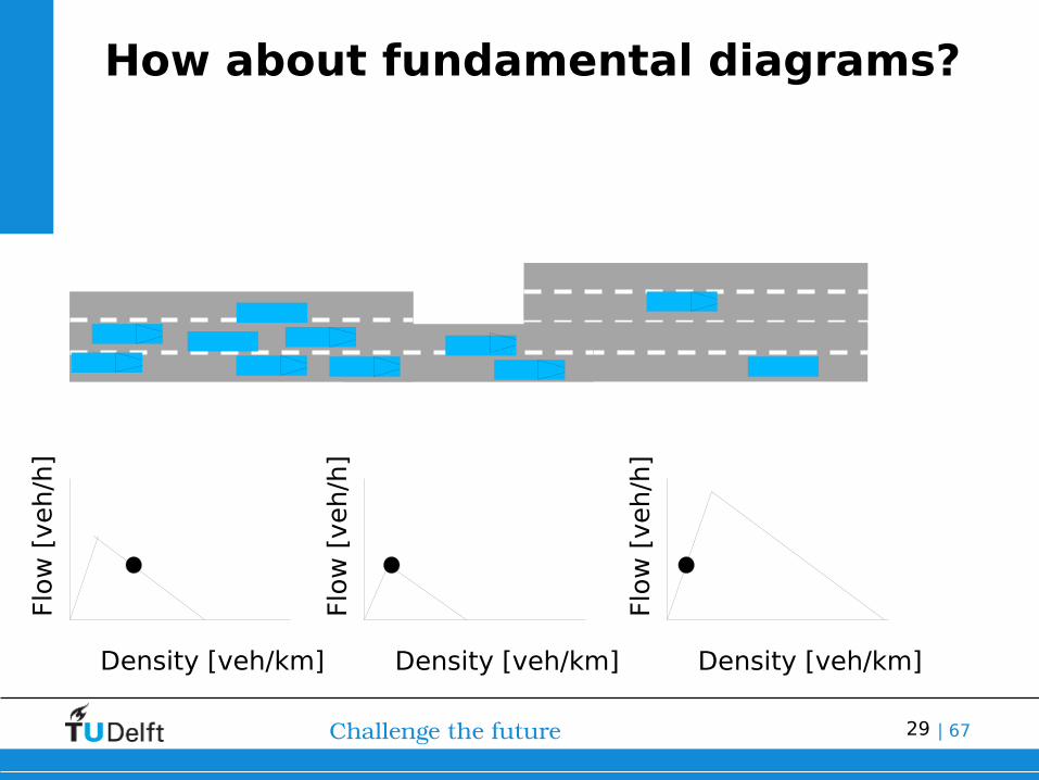
How about fundamental diagrams?
Density [veh/km]
Flow
[veh/h
]
Density [veh/km]
Flow
[veh/h
]
Density [veh/km]Fl
ow
[veh/h
]

28Challenge the future | 67
How about fundamental diagrams?
Density [veh/km]
Flow
[veh/h
]
Density [veh/km]
Flow
[veh/h
]
Density [veh/km]Fl
ow
[veh/h
]
29Challenge the future | 67
How about fundamental diagrams?
Density [veh/km]
Flow
[veh/h
]
Density [veh/km]
Flow
[veh/h
]
Density [veh/km]Fl
ow
[veh/h
]

30Challenge the future | 67
In excessive demand, where is the queue?
Density [veh/km]
Flow
[veh/h
]
Density [veh/km]
Flow
[veh/h
]
Density [veh/km]Fl
ow
[veh/h
]

31Challenge the future | 67
Simple road with increasing demand
What happens if the demand increases

32Challenge the future | 67
What observations can be made?
Density k (veh/km)
Flo
w q
(veh/h
)
A) Whole FDB) Increasing part of FD (free flow)C) Decreasing part of FD (congestion)

33Challenge the future | 67
Simple road with varying demand
Density k (veh/km)
Flo
w q
(veh/h
)

34Challenge the future | 67
Part 3: Network description

35Challenge the future | 67
● Speed in the zone dependent on nr of vehicles
Zones
Microscopic
Macroscopic
Traditional New
Zone description
Voorstel/kandidaat/utilisatie

36Challenge the future | 67
Stochasticity in local data
• Macroscopic fundamental diagram• “Average” fundamental diagram for an area
Fig: (Geroliminis and Daganzo)
Density Average density
•(A
vg
.) F
low
=>

37Challenge the future | 67
Not so simple road
• Origins and destinations everywhere
• By increasing input => congestion
• Major difference with road!

38Challenge the future | 67
Averaging traffic states leads to lower FD
Density k (veh/km)
Flo
w q
(veh
/h)

39Challenge the future | 67
Averaging traffic states leads to lower FD
But there is much more...

40Challenge the future | 67
Network with periodic boundary
1 2 3 4 1
9 10 11 12 9
5 6 7 88
13 14 15 1616
14 16
1 3
1 2 3 4 1
9 10 11 12 9
5 6 7 88
13 14 15 1616
14 16
1 3
1 2 3 4 1
9 10 11 12 9
5 6 7 88
13 14 15 1616
14 16
1 3
1 2 3 4 1
9 10 11 12 9
5 6 7 88
13 14 15 1616
14 16
1 3

41Challenge the future | 67
Build up of congestion

42Challenge the future | 67

43Challenge the future | 67

44Challenge the future | 67
Fitting a functional form
P(A)=A*(c1+c2A+c3A2)-c4
Homogeneous traffic situation
Inhomogeneous traffic situation

45Challenge the future | 67
Fitting a functional form
P(A)=A*(c1+c2A+c3A2)-c4

46Challenge the future | 67
Causes of decrease with inhomogeneity
Create GNFD without dynamics

47Challenge the future | 67
Improvement: Generalised NFD
Accumulation =>
Std
of
den
sity
=>

48Challenge the future | 67
Use for your desktop
1
5
4
3
2

49Challenge the future | 67
Part 4: Traffic dynamics

50Challenge the future | 67
Why numerical solutions are needed
● Only applicable in relatively simple situations, e.g. with respect to upstream traffic demand, off-ramps and on-ramps, etc.
● What to do when demand on main-road and on-ramps is changing dynamically? Use numerical approximations!
● Practical applications, e.g. use for network simulation
51Challenge the future | 67
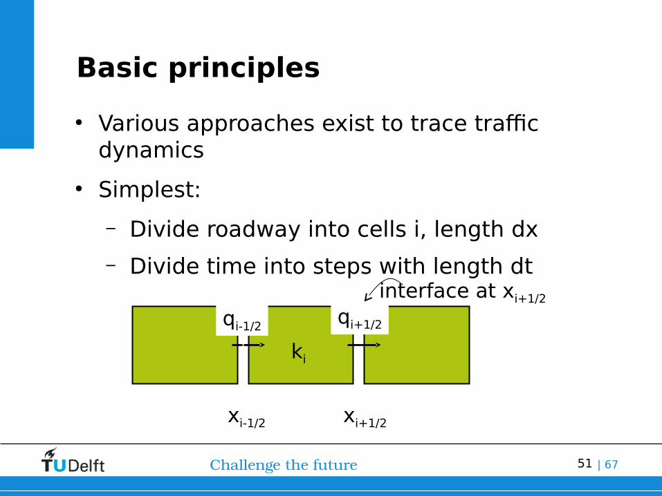
Basic principles
● Various approaches exist to trace traffic dynamics
● Simplest:
– Divide roadway into cells i, length dx
– Divide time into steps with length dt
xi-1/2 xi+1/2
ki
qi+1/2qi-1/2
interface at xi+1/2

52Challenge the future | 67
Assumptions
● Cells are homogeneous, length dx
● Within a time step (dt) , traffic flow is stationary
● Express ki,t+1 = f(ki,t,qi-1/2,t,qi+1/2,t,dt,dx)
xi-1/2 xi+1/2
ki
qi+1/2qi-1/2

53Challenge the future | 67
Basic principles (2)
● For the slides: this is the answer…
ki,t+1 = ki,t+(qi-1/2,t-qi+1/2,t)*dt/dx
● But how to get to:
i 1/ 2,j i,j i 1,j i,j 1 i 1,j 1q q(k ,k ,k ,k )
i 1/ 2,j i,j i,j i,jq k u Q k

54Challenge the future | 67
What if uncongested?
● What determines the flow from A to B?
• A – state in cell A
• B – state in cell B
ck
x
qA,B
kA,u
Ak
B,u
B

55Challenge the future | 67
What if congested?
● What determines the flow from A to B?
• A – state in cell A
• B – state in cell B
ck
x
kA,u
Ak
B,u
B
qA,B

56Challenge the future | 67
The trick:
● Demand of region A and supply of region B
● DL = maximum flow out of region L (bounded by the capacity of the road)
● SR = maximum flow into region R (bounded by road capacity and the space becoming available during one time-step)
● Actual flow at x=0 : min(DL,SR)
DL
q
Ak k
c
c k kc
S
B
c k kc
qB
k kc

57Challenge the future | 67
Graphically
• Flow based onDemand & Supply
• => fundamental diagram

Dynamic MFD modelNetwork Transmission model

59Challenge the future | 67
Network-wide traffic management
• Microscopic and macroscopic models are OK to simulate small sections
• In cities, congestion spreads and the whole city need to be described
• Another way of describing is needed

60Challenge the future | 67
Network Transmission Model
Base qualities
• Compuational speed: few steps
• Dynamic traffic patterns- Road closure, rerouting
• Schalability- bigger or smaller zones- use other scale within one zone

61Challenge the future | 67
• Implementation in OpenTraffic Sim, TU Delft simulator, enabeling link to other models
• Link to static model: ao zone-boundaries, road length per zone
Process

62Challenge the future | 67
Oorspronkelijke zones

63Challenge the future | 67
Zones

64Challenge the future | 67
Calibration
• Data shows incomplete and biassed view(location of measurements, roads?)=> no proper NFDs
• Estimate model parametersbased on theoretical considerations

65Challenge the future | 67
Solution:
• 1st estimate for NFD: based on properties of road(from static model)
• Then adapt based on speeds
• Adapt as well:boundary capacity
Density
Flo
w
Avg densityAvg
flo
w
# veh
# ex
its/Trip lengthx road length

66Challenge the future | 67
Result:
• Dynamic model voor:
1) Normal day
2) Beach traffic (adapt OD matrix)
3) Normal day with incident (capacity adapted)

67Challenge the future | 67
Learning goals
• After this lecture, the students are able to:
- describe the traffic on a microscopic and macroscopic level
- apply the relationship q=ku
- draw the fundamental diagram, i.e. q=q(k)
- argue the differences and similarities between relationships on the network level and road level
- explain the steps in numerical traffic flow models

68Challenge the future | 67
Model: possibilities
• Fast: 15s for 3 h simulation on (old) laptop. Expected: factor 10 improvement by recoding?Fast enough for on-line computation (including optimalisation!)
• Change OD matrix for events
• Boundary capacity and zone properties change, for instance in incident
• Schaling: - zone size (bigger / smaller) (?)- combine with other modelling scales(eg, one zone on microscopic level)

69Challenge the future | 67
Stochasticity in local data
• Macroscopic fundamental diagram• “Average” fundamental diagram for an area
Fig: (Geroliminis and Daganzo)
Density Average density
•(A
vg
.) F
low
=>

70Challenge the future | 67
Name giving
• Macroscopic Fundamental Diagram = Network Fundamental Diagram
• Name givingAverage density = AccumulationAverage (internal) flow = productionOutflow = performance

71Challenge the future | 67
Model: volgende stappen
• Kwaliteitsmaten & -eisen definieren
• Inclusie zoekverkeer
• “Stroomwegen” apart houden
• Beperkingen in routekeus (nu alleen wel/niet tussen zones, maar geen opeenvolging: wel A=>B en B=>C, maar niet A=>B=>C)
• Hoe kunnen regelscenario’s in het model meegenomen worden: welke parameters moeten hoe aangepast worden?
• Eventueel schakelbaarheid tussen niveaus
• Data-feed en toestandsschatting (incl HB)

72Challenge the future | 67
Name giving
• Macroscopic Fundamental Diagram = Network Fundamental Diagram
• Name givingAverage density = AccumulationAverage (internal) flow = productionOutflow = performance

73Challenge the future | 67
Shape
• Qualitatively like FD (but differences...)

74Challenge the future | 67
Relation performance - production