introduction to supersymmetry martin roˇceklisa/tasi03webpagefiles/rocek.pdf · itp–sb–93–23...
TRANSCRIPT
ITP–SB–93–23
hep-th/yymmnnn
Introduction to Supersymmetry
Martin Rocek
Institute for Theoretical Physics
SUNY at Stony Brook
Stony Brook, NY 11794-3840
ABSTRACT: This is a very lightly edited version of a set of lecture notes for five
introductory lectures on supersymmetry given in June at the TASI summer school in
Boulder CO. As such, it is often pretty telegraphic. My approach is basically quite old-
fashioned, and mostly follows Superspace by Gates et al.
email: [email protected]

Table of Contents:
LECTURE I.
I. Introduction to the introduction.
II. Introduction to supersymmetry.
III. Introduction to superspace.
IV. Supersymmetry in different dimensions.
V. Explicit supersymmetry algebras in D = 4, 3, 2.
LECTURE II.
I. Introduction and summary.
II. Models: Scalar multiplets
III. Super Yang-Mills theory.
LECTURE III.
I. Preview and summary.
II. D = 4, N = 1 models.
III. D=4 Super Yang-Mills theory.
LECTURE IV.
I. Preview and summary.
II. D = 4, N = 1 sigma Models.
III. D = 3, here we come!
IV. D = 2, nous sommes ici!
LECTURE V. Quotients and Duality
I. Preview and summary.
II. Quotients.
III. Duality
IV. Geometry of N = 2 Quotients.
V. CFT Quotients.
VI. The Surreal Pun.
2
LECTURE I.
I. Introduction to the introduction.
In the first lecture, I discuss superalgebras schematically and show how to construct
representations by introducing superspace. This is a coset of the Super Poincare group
(SISO(D−1, 1)) mod the Lorentz group (SO(D−1, 1)), and is parametrized by spacetime
coordinates x and anticommuting spinor coordinates θ. Then I construct a representation
of the SISO(D − 1, 1) algebra as superdifferential operators acting on superfields Φ(x, θ).
I also find a supercovariant derivative that (anti)commutes with (super)translations and
transforms as a spinor under the Lorentz group. I use this to define a superspace measure
that allows one to construct supersymmetric actions, as well as to define components of
superfields. Next, I describe how supersymmetry varies as one changes dimension. We will
see that starting from one supercharge (N = 1) in a higher dimension, we can get several
supercharges (N > 1) in lower dimensions. Finally I’ll give the explicit supersymmetry
algebras for N = 1, 2 in D = 4, 3, 2.
II. Introduction to supersymmetry.
What is supersymmetry? It is a symmetry between bosons and fermions with fermionic
charges and fermionic parameters. Consider a schematic action
S ∼∫
(B B + F/DF ) ; (1)
Let’s look for an invariance of the form
δB = iεF
where F is commuting and ε is anticommuting. Dimensional analysis, or the form of the
3
action S implies
δF = −i(/DB)ε
What is the symmetry algebra? We compute and find
[δε , δη]B = +2εγµηDµB ⇒ Q,Q ∼ /P , (2)
where Q is the generator of supersymmetry transformations:
δB = [iεQ, B] , DµB = [iPµ, B] , etc.
Eq. (2) is what I mean by supersymmetry: A graded algebra with fermionic charges that
anticommute to give a spacetime translation. Thus, for example, the phenomenologically
generated graded symmetry that nuclear physicists call supersymmetry is not supersym-
metry in my sense: it is an internal graded symmetry, and doesn’t have the form of (2).
Why is supersymmetry interesting? There a several reasons, some mathematical, and
some physical. Historically, supersymmetry arose in two contexts: as a symmetry on the
world sheet of the NSR formulation of the superstring, which is the only known consistent
quantum theory of gravity, and as a symmetry of certain four dimensional theories; in
such supersymmetric theories, quadratic ultraviolet divergences are absent, and thus these
theories are “natural” in a certain technical sense.
III. Introduction to superspace.
Still at a schematic level, let’s construct superspace. This will give us a more or less
systematic way of studying representations of supersymmetry.
Recall how one finds representations of the Poincare group ISO(D−1, 1). One defines
spacetime as the coset ISO(D−1, 1)/SO(D−1, 1). That is, for the ISO(D−1, 1) algebra
[J, J ] ∼ iJ, [J, P ] ∼ iP, [P, P ] = 0 ,
4
we parametrize the quotient as
h(x) = eix·Pmod SO(D − 1, 1) .
We can act by left multiplication:
h(x′) = eiw·Jeix·Pmod SO(D − 1, 1) = eiw·Jeix·P e−iw·Jmod SO(D − 1, 1)
= eix·(eiw·JPe−iw·J)mod SO(D − 1, 1) = ei(e
wx)·Pmod SO(D − 1, 1)
⇒ x′ = ewx for ew the vector representation of SO(D − 1, 1) induced by the commutator
[J, P ]. Similarly,
h(x′) = eiξ·P eix·Pmod SO(D − 1, 1) = ei(ξ+x)·Pmod SO(D − 1, 1) ⇒ x′ = x+ ξ
(Linear) representations of ISO(D− 1, 1) are found by introducing fields φ(x) that trans-
form as some matrix representation of SO(D − 1, 1):
[M,φ] ∼ φ.
We define the transformation by:
φ′(x′) = ew·Mφ(x)e−w·M ,
which implies
δφ ≡ φ′(x)− φ(x) = −δx · ∂xφ+ wφ .
Identifying this as δφ = i[w · J + ξ · P, φ], we find
P = i∂x, J = ix ∧ ∂x − iM
For superspace, we just make ISO(D − 1, 1)→SISO(D − 1, 1) above; then
P → (P,Q), x→ (x, θ), ξ → (ξ, ε) .
This leads to:
P = i∂x, Q = i(∂θ −12θ/∂x), J = i(x ∧ ∂x + θσ∂θ)− iM ,
5

where σ is the spin 12 representation of the Lorentz group.
We find an important operator that (anti)commutes with Q, P by noting that left
multiplication always commutes with right multiplication:
e−εDh(x, θ) ≡ h(x, θ)eiεQ ⇒ D,Q = 0, [D,P ] = 0 .
Using the Baker-Campbell-Hausdorff theorem eAeB = eA+B+ 12 [A,B]+... we find
D = −iQ+ θ/P = ∂θ +12θ/∂x
D is the covariant generalization of ∂θ. If Φ is a superfield, so is DΦ; neither QΦ nor ∂θΦ
are (they do not transform simply under Q). D is a SO(D − 1, 1) spinor and obeys
D, D ∼ i/∂x . (3)
It has several important uses:
1) Components of a superfield are best defined by covariant expansion:
φ = Φ|, Ψ = DΦ|, . . . etc.
where | means the θ-independent projection.
2) The basic superspace invariant measure is∫dx(D)NL(Φ, DΦ, . . .)
where N is the number of (real) components of D. This is invariant because (D)N+1 ∼
∂x (because of (3)), and δL = iεQ(L) = −εD(L) + (∂xL-term).
IV. Supersymmetry in different dimensions.
Suppose we start with a basic supersymmetry algebra in some dimension D:
Q,Q ∼ /P , [J,Q] ∼ iQ, [J, P ] ∼ iP, [J, J ] ∼ iJ .
6
We can reduce to a lower D; that is we keep the following subalgebra:
P → (P, 0) , JD →(JD−n 0
0 Tn
), and all the Q′s,
where the T ’s are generators of some internal group G and the Q’s are now in (the spinor
representation of SO(D − n, 1))× (a representation of G). The remaining subalgebra is
Q,Q ∼ /P , [J, J ] ∼ iJ, [J,Q] ∼ iQ, [J, P ] ∼ iP, [T,Q] ∼ iQ, [T, T ] ∼ iT .
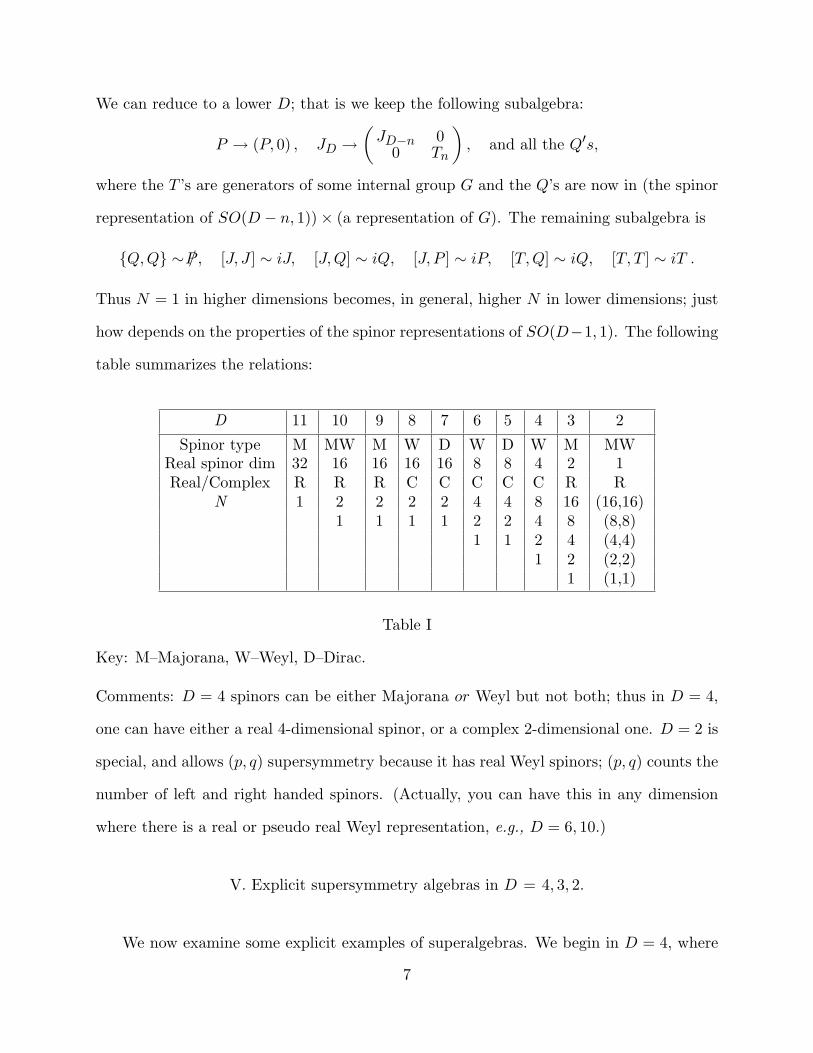
Thus N = 1 in higher dimensions becomes, in general, higher N in lower dimensions; just
how depends on the properties of the spinor representations of SO(D−1, 1). The following
table summarizes the relations:
D 11 10 9 8 7 6 5 4 3 2
Spinor type M MW M W D W D W M MWReal spinor dim 32 16 16 16 16 8 8 4 2 1Real/Complex R R R C C C C C R R
N 1 2 2 2 2 4 4 8 16 (16,16)1 1 1 1 2 2 4 8 (8,8)
1 1 2 4 (4,4)1 2 (2,2)
1 (1,1)
Table I
Key: M–Majorana, W–Weyl, D–Dirac.
Comments: D = 4 spinors can be either Majorana or Weyl but not both; thus in D = 4,
one can have either a real 4-dimensional spinor, or a complex 2-dimensional one. D = 2 is
special, and allows (p, q) supersymmetry because it has real Weyl spinors; (p, q) counts the
number of left and right handed spinors. (Actually, you can have this in any dimension
where there is a real or pseudo real Weyl representation, e.g., D = 6, 10.)
V. Explicit supersymmetry algebras in D = 4, 3, 2.
We now examine some explicit examples of superalgebras. We begin in D = 4, where
7

we have complex Weyl spinor supercharges Qα, Qα = −(Qα)† for α = (+,−). We can raise
and lower spinor indices by Cαβ = −Cβα, CαβCγβ = δγα; for example, Qα = CαβQβ , Qα =
QβCβα.* The spinors Q are in the (12 , 0) representation of SL(2C), their conjugates Q
are in the (0, 12) representation, and vectors are in the (1
2 ,12) representation. Thus vectors
are naturally described as 2 × 2 matrices. Then the N = 1 superalgebra has charges
Qα, Qα, Pαα, Jαβ , Jαβ which obey the following algebra:
Qα, Qα = Pαα ,
[Jαβ , Qγ ] =12i(CγαQβ + CγβQα) ,
[Jαβ , Pγγ ] =12i(CγαPβγ + CγβPαγ) ,
[Jαβ , Jγδ] =12i(CγαJβδ + CγβJαδ + CδαJβγ + CδβJαγ) ,
and all other commutation relations either vanish or follow by hermitian conjugation. The
spinor derivatives are:
Dα = ∂α +i
2θα∂αα, Dα = ∂α +
i
2θα∂αα
Dα, Dβ = Dα, Dβ = 0, Dα, Dα = i∂αα
The algebra for N = 2 in D = 4 is essentially the same, except that Q and D get
doubled:
Daα, Dbβ = iδba∂αβ , (a = 1, 2).
One may also include an SU(2) internal symmetry under which the Q’s transform as
isospinors.
In D = 3, for N = 2, we just drop the “ ˙ ” from N = 1 above, impose Pαβ = Pβα, and
let Jαβ be real.
For D = 3, N = 1, there is only one real Qα, and of course Pαβ and Jαβ ; the algebra
* Two frequently used identities for two component spinors are X[αβ] ≡ Xαβ − Xβα =−CαβXγ
γ and X[αβγ] = 0.
8
is:Qα, Qβ = 2Pαβ ,
[Jαβ , Qγ ] =12i(CγαQβ + CγβQα) ,
[Jαβ , Pγδ] =12i(CγαPβδ + CγβPαδ + CδαPβγ + CδβPαγ) ,
[Jαβ , Jγδ] =12i(CγαJβδ + CγβJαδ + CδαJβγ + CδβJαγ) ,
and the spinor derivatives are
Dα = ∂α + iθα∂αβ , Dα, Dβ = 2i∂αβ .
Finally, we consider D = 2. For N = (1, 1), we have the algebra of D = 3, N = 1 with
P+− = J++ = J−− = 0. This leaves Q±, P±±, J ≡ J+−; these obey
Q2± = P±± ,
[J, Q±] = ±12Q± ,
[J, P±±] = ±P±± .
The corresponding spinor derivatives are
D± = ∂± + iθ±∂±± , D2± = i∂±± .
Often, I’ll Wick rotate; then
D± = ∂± + θ±∂z,z , D2± = ∂z,z .
For N = (2, 2), we have
D± = ∂± +i
2θ±∂±± , D± = ∂± +
i
2θ±∂±± ,
with
D2± = D2
± = 0 , D±, D± = i∂++ , D+, D− = D−, D+ = 0.
The Wick rotated form is
D± = ∂± +12θ±∂z,z , D± = ∂± +
12θ±∂z,z , D±, D± = ∂z,z .
9
Finally, for N = (4, 4), we have four complex spinor derivatives D±a, Da± obeying
D±a, Db± = iδba∂±± , (a = 1, 2) .
LECTURE II.
I. Introduction and summary.
In this lecture, I construct several N = 1 models in D = 3, 2. I write down actions
in superspace, define components, and work out component actions. We will find actions
that have the usual form for bosons and fermions, but with particular couplings dictated
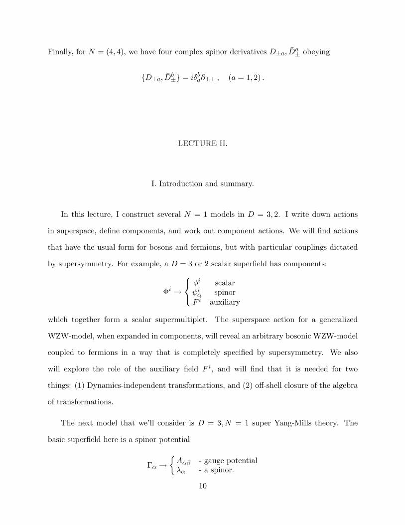
by supersymmetry. For example, a D = 3 or 2 scalar superfield has components:
Φi →
φi scalarψiα spinorF i auxiliary
which together form a scalar supermultiplet. The superspace action for a generalized
WZW-model, when expanded in components, will reveal an arbitrary bosonic WZW-model
coupled to fermions in a way that is completely specified by supersymmetry. We also
will explore the role of the auxiliary field F i, and will find that it is needed for two
things: (1) Dynamics-independent transformations, and (2) off-shell closure of the algebra
of transformations.
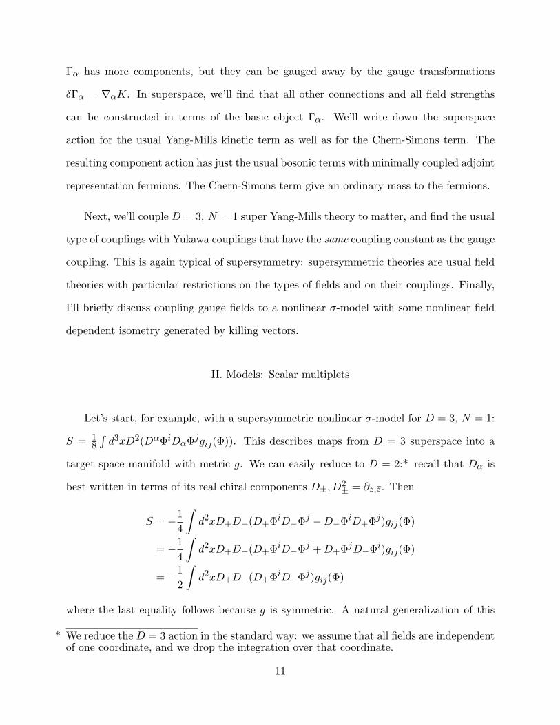
The next model that we’ll consider is D = 3, N = 1 super Yang-Mills theory. The
basic superfield here is a spinor potential
Γα →Aαβ - gauge potentialλα - a spinor.
10
Γα has more components, but they can be gauged away by the gauge transformations
δΓα = ∇αK. In superspace, we’ll find that all other connections and all field strengths
can be constructed in terms of the basic object Γα. We’ll write down the superspace
action for the usual Yang-Mills kinetic term as well as for the Chern-Simons term. The
resulting component action has just the usual bosonic terms with minimally coupled adjoint
representation fermions. The Chern-Simons term give an ordinary mass to the fermions.
Next, we’ll couple D = 3, N = 1 super Yang-Mills theory to matter, and find the usual
type of couplings with Yukawa couplings that have the same coupling constant as the gauge
coupling. This is again typical of supersymmetry: supersymmetric theories are usual field
theories with particular restrictions on the types of fields and on their couplings. Finally,
I’ll briefly discuss coupling gauge fields to a nonlinear σ-model with some nonlinear field
dependent isometry generated by killing vectors.
II. Models: Scalar multiplets
Let’s start, for example, with a supersymmetric nonlinear σ-model for D = 3, N = 1:
S = 18
∫d3xD2(DαΦiDαΦjgij(Φ)). This describes maps from D = 3 superspace into a
target space manifold with metric g. We can easily reduce to D = 2:* recall that Dα is
best written in terms of its real chiral components D±, D2± = ∂z,z. Then
S = −14
∫d2xD+D−(D+ΦiD−Φj −D−ΦiD+Φj)gij(Φ)
= −14
∫d2xD+D−(D+ΦiD−Φj +D+ΦjD−Φi)gij(Φ)
= −12
∫d2xD+D−(D+ΦiD−Φj)gij(Φ)
where the last equality follows because g is symmetric. A natural generalization of this
* We reduce the D = 3 action in the standard way: we assume that all fields are independentof one coordinate, and we drop the integration over that coordinate.
11
(special to D = 2) is
Sgen = −12
∫d2xD+D−(D+ΦiD−Φj)(gij(Φ) + bij(Φ)) (4)
where bij = −bji is an antisymmetric tensor on the target space. Let’s find the component
expansion; we define components
φi = Φi|, ψi = D+Φi|, ψi = D−Φi|, F i = iD+D−Φi| .
Then
Sgen = −12
∫d2xD+
[(−D+D−ΦiD−Φj −D+Φi∂Φj)(gij + bij)
+D+ΦiD−Φj(gij,k + bij,k)D−Φk]
= −12
∫d2x
[(− (∂ψi)ψj + F iF j − ∂φi∂φj + ψi∂ψj
)(gij + bij)
+[(−iF iψj + ψi∂φj)ψk + (∂φiψj + iψiF j)ψk − iψiψjF k
](gij,k + bij,k)
+ ψiψjψlψk(gij,kl + bij,kl)],
where gij,k = ∂∂φk gij , etc. We collect terms and integrate by parts to get:
S =12
∫d2x
[∂φi∂φj(gij + bij)− (ψi∇ψj + ψi∇ψj)gij
− 12R−ij,klψ
iψjψkψl − gij(Fi + iΓ−ilk ψ
lψk)(F j + iΓ−jmnψmψn)]
where∇ψi = ∂ψi + Γ+i
jk ∂φjψk
∇ψi = ∂ψi + Γ−ijk∂φjψk
.
R−ijkl is the Riemann curvature of Γ−, and
Γ±ljk =ljk
± gli
12(bij,k + bjk,i + bki,j)︸ ︷︷ ︸
Tijk the torsion
(5)
This is an N = 1 supersymmetric generalized WZW model. We will discuss this model
later at great length, but let me make one comment here: if R− = 0, then this is precisely
a Wess-Zumino-Witten (WZW) model.
12
We can also add a superpotential:
i
∫d2xD+D−V (Φ) =
∫d2xV,iF
i + iV,ijψiψj
Finally, lets find the supersymmetry transformations of the components:
δφi = −(ε+Q− − ε−Q+)Φi| = i(ε+D− − ε−D+)Φi| = i(ε+ψi − ε−ψi)
(recall D = −iQ+ 2θP )
δψi = −(ε+Q− − ε−Q+)D+Φi| = i(ε+D− − ε−D+)D+Φi|
= −(ε+F i + iε−∂zφi)
What is F i? Note that it enters the action only algebraically . It is called an auxiliary field.
It plays a very interesting role; its transformation is:
δF i = −(ε+Q− − ε−Q+)(iD+D−Φi)| = (ε+D− − ε−D+)D+D−Φi|
= −(ε+∂ψi + ε−∂ψi) .
Note that δφi, δψi, and δF i are independent of the form of S; the transformations are valid
without the use of field equations, and the algebra closes without any field equations. If we
eliminate F i by its equation of motion, F i = −iΓ−ilk ψlψk, then δψi depends on Γ−, which
in turn depends on the form of S. Consider the simplest example: g + b = 1,Γ = R = 0.
Then on-shell F i = 0, and δψi = −iε−∂zφi. Let’s check the algebra; on φ, we find
[δε, δη]φi = 2i(η+(iε+∂φi)− η−(−iε−∂φi))
= +2(ε+η+∂φi + ε−η−∂φi) ,
which is fine. However, on ψi we have:
[δε, δη]ψi = −iη−∂(iε+ψi − iε−ψi)− η ↔ ε
= +2ε−η−∂ψi + (η−ε+ − ε−η+)∂ψi
= 2(ε+η+∂ + ε−η−∂)ψi︸ ︷︷ ︸good
− 2ε+η+∂ψi + (η−ε+ − ε−ψ+)∂ψi︸ ︷︷ ︸Field equations
13
Without auxiliary fields, in general, the algebra only close on-shell , that is, modulo equa-
tions of motion. Note that the action is still invariant without any equations of motions;
since these are defined by extremizing the action, they can never be used in verifying a
symmetry. Sadly, there are supersymmetric systems that we don’t really understand in
superspace, i.e., we only have on-shell representations of the algebra.
We will eventually run into this, but let me say now that this is typically the situation
for high D and/or N .
Another comment, referring back to off-shell supersymmetry transformations: how do
you break supersymmetry ? Well, you need 〈δ(something)〉 6= 0. Note that⟨φi
⟩6= 0 does
not break supersymmetry (φ enters the transformation laws only through its derivatives),
but⟨F i
⟩6= 0 does. This is a very generic feature.
III. Super Yang-Mills theory.
Let’s look at some more models. Back in D = 3, N = 1, we can consider Super
Yang-Mills theory. We do this by covariantizing the spinor derivative Dα:
Dα → ∇α ≡ Dα − iΓα .
We can construct everything in terms of the basic object Γα. For example, we can define
the vector potential Γαβ by
∇α,∇β = 2i∇αβ ≡ 2i(∂αβ − iΓαβ) ⇒ Γαβ = −12(iD(αΓβ) + Γα,Γβ)
(which means we absorb Fαβ into Γαβ). The components follow from the pieces of Γα that
remain after we use the gauge transformation
δΓα = ∇αK
14

as follows:K| is the component gauge parameter
∇αK| gauges away Γα|
∇2K| gauges away DαΓα|This leaves the component gauge field Aαβ and spinor λβ :
D(αΓβ)| ∼ Aαβ DαDβΓα| ∼ λβ .
A more careful definition of the components is given below.
The Bianchi identities
[∇(α∇β ,∇γ)] = 0
imply
[∇α,∇βγ ] ≡ −iFα,βγ = Cα(βFγ)
(that is F(α,βγ) = 0), which allows us to compute the superfield strength
Fα =13
(i(DβΓαβ − ∂αβΓβ) + [Γβ ,Γαβ ]
).
We also can find the usual field strength as follows:
[∇αβ ,∇γδ] = − i2[∇αβ , ∇γ ,∇δ] =
i
2(∇γ , [∇δ,∇αβ ]+ ∇δ, [∇γ ,∇αβ ]) ,
and hence
[∇αβ ,∇γδ] =i
2
(Cδα∇γFβ + Cδβ∇γFα + Cγα∇δFβ + Cγβ∇δFα
)=−i4
[(Cαγ(∇βFδ +∇δFβ) + α↔ β
)+ γ ↔ δ
] .
Thus we have found the spacetime Yang-Mills field strength in terms of the spinor field
strength Fα.* (Note that we also have:∇α, [∇β ,∇αβ ] = 0 and hence ∇αFα = 0.)
For an action, we have:
S =14
∫d3xDαDα
1g2Tr(F
βFβ) .
* We use the two component spinor identities from the footnote of Section V, Lecture I.
15
We can also add a super Chern-Simons term:
SCS =12
∫d3xDαDα
m
g2Tr(Γβ(Fβ −
16[Γγ ,Γβγ ])) .
This is, of course, a special feature of D = 3. We can define components by projection as
follows: The gauge field is
Γαβ | = Aαβ ,
which leads to a component field strength
∼ ∇(αFβ)| .
The physical spinor is
Fα| = λα|.
As described above, the rest of Γα can be gauge away.
In components, the sum of the two actions is simply a Yang-Mills field coupled to
a massive adjoint representation spinor with mass equal to the topological mass of the
Yang-Mills field given by the Chern-Simons term.
Finally, let us consider matter couplings; that is, for some scalar fields transforming as
δΦi = i(KΦ)i ≡ iKA(TAΦ)i we couple to Yang-Mills fields by the usual minimal coupling
prescription: DαΦi → (∇αΦ)i = DαΦi − i(ΓαΦ)i. This gives rise to a matter action
S = −18
∫d3xDαDα
[(∇βΦ)i(∇βΦ)i
]=
18
∫d3xDαDα
[Φi(∇β∇βΦ)i
]=
18
∫d3x
[∇α∇α
(Φi(∇β∇βΦ)i
)]=
18
∫d3x
[(∇α∇αΦ)i(∇β∇βΦ)i + 2(∇αΦ)i(∇α∇β∇βΦ)i + Φi(∇α∇α∇β∇βΦ)i
]=
12
∫d3x
[14FiF
i − iψαi (∇αβψβ)i − 12(∇αβφ)i(∇αβφ)i + i(ψαi (λαφ)i − φi(λ
αψα)i)]
with F i auxiliary again. More generally, we can consider an isometry that acts on some
scalar fields by δΦi = KAXiA(Φ), where Xi
A are killing vectors satisfying
Xi;j +Xj;i = 0 .
16

This leaves the action S =∫d3xDαDαgijD
βΦiDβΦj invariant, as can be seen as follows:
δS =∫d3xDαDα
(2gijD
βΦiDβ(KAXjA) + gij,kD
βΦiDβΦjKAXkA
)=
∫d3xDαDα
(2KADβΦiDβΦjXAi;j −DβΦiDβΦjKAXk
A(gij,k + gik,j − gjk,i)
+ gij,kDβΦiDβΦjKAXk
A
)= 0 .
Now minimal coupling takes the form (∇αΦ)i = DαΦi − iΓAαXiA(Φ).
LECTURE III.
I. Preview and summary.
I describe D = 4, N = 1 supersymmetric models, in particular, I write down the most
general renormalizable D = 4 supersymmetric model. This will involve scalar multiplets
and Yang-Mills theories.* However, the superspace formulation of these theories is quite
different from the D = 3, N = 1 theories described in the previous lecture. We will see
that we will have to introduce superfields that are independent of some θ’s — constrained
superfields. These exist for D = 4, N = 1 because the superderivatives have an abelian
subalgebra (that is not real). These “chiral” superfields resemble complex D = 3, N = 1
scalar superfields, and describe matter supermultiplets with a complex scalar, a Weyl
spinor, and a complex auxiliary field. The Yang-Mills multiplets are described by an
unrestricted superfield. The structure of the theory is somewhat novel and is determined
by the structure of the matter multiplets: that is, by the principle that the restricted
(chiral) superfields that we use to describe matter should be allowed to carry Yang-Mills
charge.
* Supersymmetric standard models are of this form; so is the only (proven) finite D = 4theory, N = 4 Super Yang-Mills theory.
17
II. D = 4, N = 1 models.
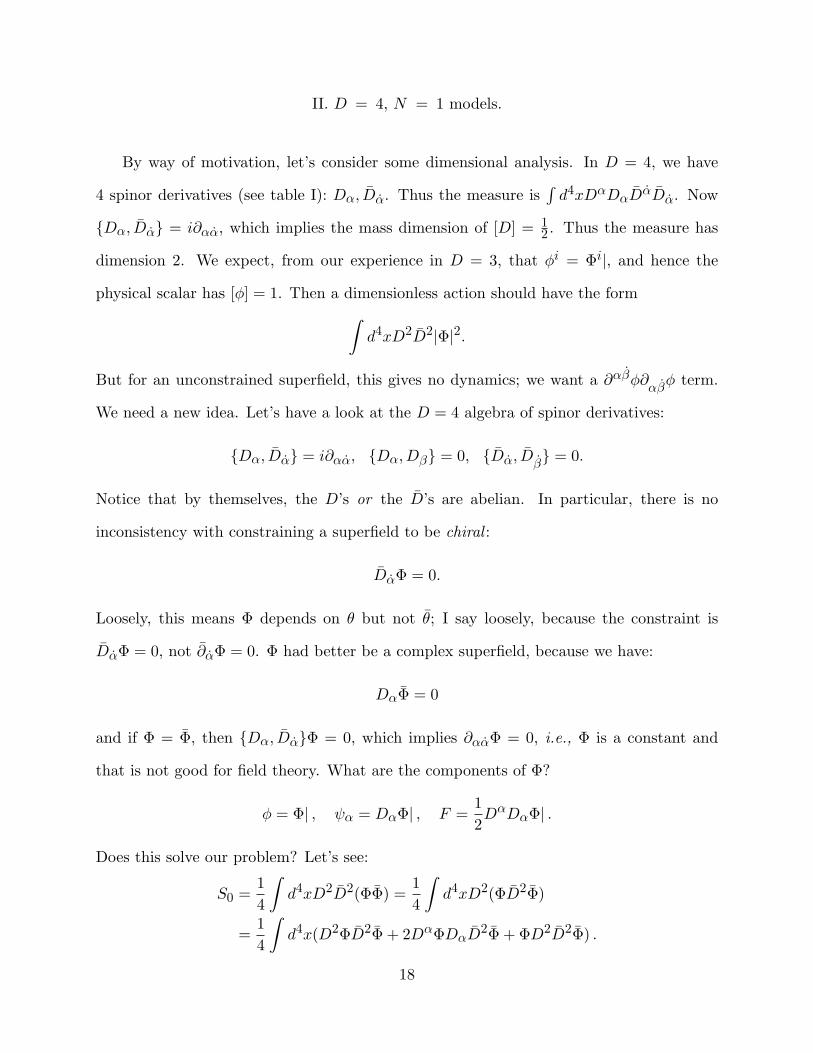
By way of motivation, let’s consider some dimensional analysis. In D = 4, we have
4 spinor derivatives (see table I): Dα, Dα. Thus the measure is∫d4xDαDαD
αDα. Now
Dα, Dα = i∂αα, which implies the mass dimension of [D] = 12 . Thus the measure has
dimension 2. We expect, from our experience in D = 3, that φi = Φi|, and hence the
physical scalar has [φ] = 1. Then a dimensionless action should have the form∫d4xD2D2|Φ|2.
But for an unconstrained superfield, this gives no dynamics; we want a ∂αβφ∂αβφ term.
We need a new idea. Let’s have a look at the D = 4 algebra of spinor derivatives:
Dα, Dα = i∂αα, Dα, Dβ = 0, Dα, Dβ = 0.
Notice that by themselves, the D’s or the D’s are abelian. In particular, there is no
inconsistency with constraining a superfield to be chiral :
DαΦ = 0.
Loosely, this means Φ depends on θ but not θ; I say loosely, because the constraint is
DαΦ = 0, not ∂αΦ = 0. Φ had better be a complex superfield, because we have:
DαΦ = 0
and if Φ = Φ, then Dα, DαΦ = 0, which implies ∂ααΦ = 0, i.e., Φ is a constant and
that is not good for field theory. What are the components of Φ?
φ = Φ| , ψα = DαΦ| , F =12DαDαΦ| .
Does this solve our problem? Let’s see:
S0 =14
∫d4xD2D2(ΦΦ) =
14
∫d4xD2(ΦD2Φ)
=14
∫d4x(D2ΦD2Φ + 2DαΦDαD2Φ + ΦD2D2Φ) .
18

We need a few identities:
DαD2 = D2Dα − 2i∂ααD
α
and
D2D2Φ = 2∂αα∂ααΦ
which implies
S0 =∫d4x(FF − iψα∂ααψ
α +12φ∂αα∂ααφ) ,
which is just what we want! Other constraints are possible; there is a systematic way to
study all linear constraints, but it is far too technical to describe here (see Gates et al.,
section 3.11.a).
How about masses and interactions? Well, now we’re hoisted by our own petard:∫d4xD2D2|Φ|2 is a kinetic term, not a mass! How do we get no derivatives? We need a
new superspace measure. We can get a clue as follows: The kinetic action can be written
as∫d4xD2(ΦD2Φ); this almost looks like D = 3. Can we use D2 as a measure? Not in
general, but for Lagrangians that are chiral, we can!
This leads to the following theorem:
For L such that DL = 0, Schiral =∫d4xD2L is a superinvariant.
Proof:δSchiral = i
∫d4xD2(εαQα + εαQα)L
= −∫d4xD2(εαDα + εαDα)L+ total derivatives
=∫d4xD2Dα(εαL) = 0 ,
where the last equality follows from D3 = 0.∫d4xD2 is a chiral measure good for chiral
Lagrangians. Now we’re in great shape:
SV =12
∫d4xD2V (Φi) + c.c.
=∫d4x(V,iF
i +12V,ijψ
iαψjα) + c.c.
19

For V = 12mΦ2 + 1
3!λΦ3, we get
Sm,λ =∫d4x
[m(
12ψαψα + φF ) +
12λ(φψαψα + Fφ2) + c.c.
](There is an old nomenclature that is still used: terms constructed with
∫d4xD2D2 are
called “D” terms, whereas terms constructed with∫d4xD2 + c.c. are called “F” terms.)
Eliminating F , we get∫d4x
[φ(
12∂αα∂αα −m2)φ− iψα∂ααψ
α +12m(ψαψα + ψαψα)
− 12mλ(φφ2 + φφ2)− 1
4λ2φ2φ2 +
12λ(φψαψα + φψαψα)
]This is the most general renormalizable supersymmetric model with one complex scalar φ
and one Weyl spinor ψ.
We can easily generalize to many Φ’s:
S =∫d4xD2D2ΦiΦi +
∫d4xD2V (Φi) +
∫d4xD2V (Φi)
for V (Φi) a cubic polynomial.
III. D=4 Super Yang-Mills theory.
As for the scalar multiplet, we immediately have a problem: where can we start? We
can’t use minimal coupling, as there are no derivatives in the Lagrangian! Let’s examine
the constraints on the matter superfields. Suppose we start with a chiral superfield; we
may ask that it remain chiral after a gauge transformation. This implies that the gauge
parameter must be chiral:
DαΦi = 0 ; we ask Dα(δΦi) = 0 , but δΦi = iΛA(TA)ij︸ ︷︷ ︸Λi
j
Φj ,
which implies that Λ better be chiral. This implies, however, that Dα is gauge-covariant
as it stands:
δ(DαΦi) = Dα(iΛijΦj) = iΛijDαΦj .
20
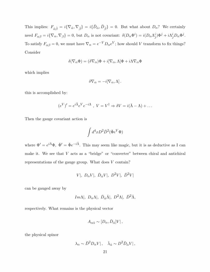
This implies: Fαβ
= i∇α,∇β = iDα, Dβ = 0. But what about Dα? We certainly
need Fαβ = i∇α,∇β = 0, but Dα is not covariant: δ(DαΦi) = i(DαΛij)Φj + iΛijDαΦj .
To satisfy Fαβ = 0, we must have ∇α = e−VDαeV ; how should V transform to fix things?
Consider
δ(∇αΦ) = (δ∇α)Φ + i[∇α,Λ]Φ + iΛ∇αΦ
which implies
δ∇α = −i[∇α,Λ] .
this is accomplished by:
(eV )′ = eiΛeV e−iΛ , V = V † ⇒ δV = i(Λ− Λ) + . . .
Then the gauge covariant action is∫d4xD2D2(ΦeV Φ)
where Φ′ = eiΛΦ, Φ′ = Φe−iΛ. This may seem like magic, but it is as deductive as I can
make it. We see that V acts as a “bridge” or “converter” between chiral and antichiral
representations of the gauge group. What does V contain?
V |, DαV |, DαV |, D2V |, D2V |
can be gauged away by
ImΛ|, DαΛ|, DαΛ|, D2Λ|, D2Λ,
respectively. What remains is the physical vector
Aαα ∼ [Dα, Dα]V | ,
the physical spinor
λα ∼ D2DαV | , λα ∼ D2DαV | ,
21

and a hermitian auxiliary field:
D ∼ DαD2DαV | .
The full nonlinear expressions for these components can be found from the Bianchi iden-
tities and the constraints:
∇α,∇β = ∇α, ∇β = 0 , ∇α, ∇α = i∇αα .
The first two constraints can be interpreted as integrability conditions for the existence
of chiral and anti-chiral superfields, and the third is merely a matter of convenience: it
defines the vector connection in terms of the spinor connections, just as in D = 3. The
Bianchi identities now imply:
[∇α,∇ββ ] = CαβWβ , Wβ =
i
2DαDα(e−VDβe
V )
The covariant expressions for the components of the Yang-Mills multiplet are:
Aαα = Γαα| , λα = Wα| , λα = Wα| ,
D = ∇αWα| , fαβ ≡ ∂ααAβα + ∂β
αAαα = ∇(αWβ)| .
We note that DαWβ = 0. This allows us to write a consistent gauge invariant action for
the Yang-Mills field:
SYM =1
4g2 tr
∫d4xD2(WαWα) .
This is real up to a topological FF term. We can also add a term∫d4xD2D2tr(νV )
for an abelian subgroup; I’ll leave it as an exercise to prove that this is gauge invariant
when ν commutes with all the TA’s. Such a term is called the Fayet-Illiopoulos term, and
leads to spontaneous supersymmetry breaking.
22
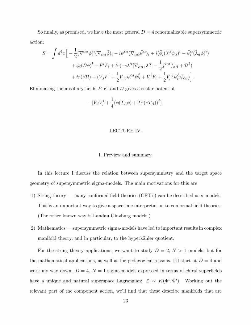
So finally, as promised, we have the most generalD = 4 renormalizable supersymmetric
action:
S =∫d4x
[− 1
2(∇ααφ)i(∇ααφ)i − iψαi(∇ααψα)i + i(φi(λ
αψα)i − ψαi (λαφ)i)
+ φi(Dφ)i + F iFi + tr(−iλα[∇αα, λα]− 12fαβfαβ +D2)
+ tr(νD) + (V,iFi +
12V,ijψ
αiψjα + V i, Fi +
12V ij, ψ
αi ψαj)
].
Eliminating the auxiliary fields F, F , and D gives a scalar potential:
−[V,iVi, +
14(φ(TAφ) + Tr(νTA))2].
LECTURE IV.
I. Preview and summary.
In this lecture I discuss the relation between supersymmetry and the target space
geometry of supersymmetric sigma-models. The main motivations for this are
1) String theory — many conformal field theories (CFT’s) can be described as σ-models.
This is an important way to give a spacetime interpretation to conformal field theories.
(The other known way is Landau-Ginzburg models.)
2) Mathematics — supersymmetric sigma-models have led to important results in complex
manifold theory, and in particular, to the hyperkahler quotient.
For the string theory applications, we want to study D = 2, N > 1 models, but for
the mathematical applications, as well as for pedagogical reasons, I’ll start at D = 4 and
work my way down. D = 4, N = 1 sigma models expressed in terms of chiral superfields
have a unique and natural superspace Lagrangian: L ∼ K(Φi, Φi). Working out the
relevant part of the component action, we’ll find that these describe manifolds that are
23
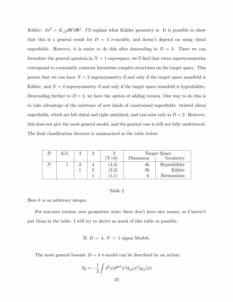
Kahler : ds2 = K,idΦidΦj . I’ll explain what Kahler geometry is. It is possible to show
that this is a general result for D = 4 σ-models, and doesn’t depend on using chiral
superfields. However, it is easier to do this after descending to D = 3. There we can
formulate the general question in N = 1 superspace; we’ll find that extra supersymmetries
correspond to covariantly constant hermitian complex structures on the target space. This
proves that we can have N = 2 supersymmetry if and only if the target space manifold is
Kahler, and N = 4 supersymmetry if and only if the target space manifold is hyperkahler.
Descending further to D = 2, we have the option of adding torsion. One way to do this is
to take advantage of the existence of new kinds of constrained superfields: twisted chiral
superfields, which are left chiral and right antichiral, and can exist only in D = 2. However,
this does not give the most general model, and the general case is still not fully understood.
The final classification theorem is summarized in the table below:
D 6/5 4 3 2 Target Space(T=0) Dimension Geometry
N 1 2 4 (4,4) 4k Hyperkahler1 2 (2,2) 2k Kahler
1 (1,1) k Riemannian
Table 2
Here k is an arbitrary integer.
For non-zero torsion, new geometries arise; these don’t have nice names, so I haven’t
put them in the table. I will try to derive as much of this table as possible.
II. D = 4, N = 1 sigma Models.
The most general bosonic D = 4 σ-model can be described by an action:
S0 = −12
∫d4x(∂ααφi∂ααφ
j)gij(φ)
24
and describes maps from 4 dimensions into a target space with a metric gij . On dimensional
grounds (counting D’s), the superspace analog for chiral superfields must be:
S =14
∫d4xD2D2K(Φi, Φi) , DαΦi = DαΦi = 0.
Let’s work out the terms in this corresponding to S0:
S =14
∫d4x
(KiD
2D2Φi − 2Kı(DαDαΦi)(DαDαΦj)
+ F terms + ψ terms)|
=12
∫d4x(Kı∂
αα∂ααφi +Kı∂
ααφi∂ααφj) + . . .
= −12
∫d4xKıj∂
ααφi∂ααφj + . . .
,
where we have integrated by parts in the last step. Thus the metric gij is written as the
matrix of second derivatives of the function K:
gij ∼∂2K
∂φi∂φj, ds2 = Kidφ
idφj
This is the form of an arbitrary Kahler metric. Notice that the geometry depends only
on the Hessian of K; in particular, shifting K by the real part of a holomorphic function
f(φ)+ f(φ) does not change the metric. This is also true for the superspace action, because
the full superspace measure∫d4xD2D2 annihilates a chiral or antichiral integrand.
We have shown that for chiral superfields, the N = 1, D = 4 target space must be
Kahler; conversely, for any Kahler manifold, we can write an N = 1, D = 4 σ-model in
terms of chiral superfields. This result is originally due to Zumino. To proceed further,
we need to know more about Kahler geometry. Notice that the manifold is complex: the
coordinates can be chosen to be complex (φ and φ). This gives an intuitive explanation of
why supersymmetry knows about target space geometry: chiral superfields correspond to
complex coordinates.
We can define a natural tensor:
Jji = iδ
ji , J
ji = J
jı = 0, J ı = −iδı .
25

Then J has the following important properties:
0. The manifold on which it is defined is even (real) dimensional.
1. J2 = −1 (J is an almost complex structure).
2. Let ∂±I = ∂I ± iJJI ∂J , I = i, j. Then [∂±I , ∂±J ] = CKIJ∂±K (J is an integrable
complex structure.)
3. gIJJJK = −gKJJJI (The metric is hermitian.)
4. ∇IJJK = 0 (J is covariantly constant).
5. This implies [∇I ,∇J ]JKL = 0, which further implies
6. RIJKMJML + RIJLMJKM = 0 (The holonomy of the Levi-Civita connection is not
O(2K) but U(K).)
These properties characterize Kahler manifolds.
III. D = 3, here we come!
As described in the first lecture, we can reduce to D = 3. We let:
Dα → Dα, Dα → Dα, ⇒ Dα, Dβ = i∂αβ = i∂βα .
The action remains
S =14
∫d3xD2D2K(Φi, Φi), DαΦi = DαΦi = 0
But, because we’re in D = 3, we can write N = 1 σ-models:
S =18
∫d3xD2
(DαΦiDαΦjgij(Φ)
)(Recall lecture 2). Here, i, j are real indices. For future use we write down the superfield
equation of motion: DαDαΦi + ΓijkDαΦjDαΦk = 0.) Let’s try and see what happens
26

if we look for a second supersymmetry using N = 1 components. We want it to anti-
commute with the first supersymmetry , so we should write it with Dα; the most general
transformation that we can write down is:
δΦi = J ijεαDαΦj ; (6)
let’s study the consequences of
(A) imposing the supersymmetry algebra on Eq. (6); this will lead to conditions 0.+1.+2.
above, and hence to the conclusion that the target space manifold is complex.
(B) imposing invariance of S on Eq. (6); this will lead to 3. + 4., and to the conclusion
that the manifold is Kahler.
(A) Starting only from the supersymmetry algebra, we have
[δε, δη]Φi = J ijηαDα(Jjkε
βDβΦk) + J ij,kJkl (εβDβΦl)(ηαDαΦj)− η ↔ ε
= −J ijJjkηαεβDα, DβΦk − J ijJ
j[k,l]η
αεβDαΦlDβΦk
+ J i[j|,kJk|l]η
αεβDβΦlDαΦj
which leads to
−J ijJjk = δik ⇒ (conditions 0.+ 1.) ,
and
J ijJj[k,l] + J
j[kJ
il],j = 0 ⇒ (condition 2.) .
(B) Invariance of the action implies:
0 = δS =18
∫d3xD2
[− 2εβ(DβΦl) J il gij︸ ︷︷ ︸
Jjl
(DαDαΦi + ΓijkDαΦjDαΦk)
].
A nontrivial calculation reveals that this vanishes if and only if Jil = −Jli, which implies
condition 3. (the metric is hermitian), and if Jil,k − JijΓjlk − JjlΓ
jik = 0, which implies
condition 4. (the metric is Kahler).
27

So any N = 2, D = 3 model is Kahler, and hence can be written with chiral superfields,
and hence the same is true for any N = 1, D = 4 model.
How about N = 3, D = 3? This means there are two complex structures J1, J2, and
the metric is Kahler with respect to both of them. Imposing the supersymmetry algebra
implies [δ1, δ2] = 0 and hence J1J2 +J2J1 = 0. This implies that (J1J2)2 = −1, and hence
J3 ≡ J1J2
is another complex structure, and generates yet another symmetry (it is easy to show J3
is hermitian and covariantly constant). So N = 3 ⇒ N = 4, and the target space manifold
is hyperkahler. Hyperkahler geometry is characterized by the existence of 3 covariantly
constant complex structures Jx, obeying the algebra of the imaginary quaternions:
Jx, Jy = −2δxy .
IV. D = 2, nous sommes ici!
We now reduce once more to reach two dimensions. The resulting algebra of spinor
derivatives is:
D2+ = D2
− = D+, D− = D+, D− = 0 , D+, D+ = ∂, D−, D− = ∂ .
Again, we can define a chiral superfield that obeys: D±Φ = 0. But in D = 2, and only in
D = 2, D+, D− = 0, so we can also have twisted chiral superfields:
D+χ = D−χ = 0 ,
D+χ = D−χ = 0 .
Now let’s consider ∫d2xD2D2K(Φi, χa) .
28

by the usual manipulations, this gives a bosonic part with a metric and in addition an
antisymmetric tensor b-field:
gi = Ki, gab = −Kab, bia = −Kia, baı = Kaı.
Two obvious questions arise: is this the most general (2,2) model? What kind of geometry
describes its target space?
To get an answer, we go back to N = 1 superspace. Because we are in D = 2, we can
have separate left and right handed transformations with parameters ε+ and ε−:
δΦI = J(+)IJ ε+D+ΦJ + J
(−)IJ ε−D−ΦJ . (7)
Now we impose the supersymmetry algebra, and find
1. J2(±) = −1.
2. J(±) are integrable.
3. There is a term that involves the field equations and [J(+), J(−)]:
[δ(+),δ(−)]ΦI
= δ(+)(J(−)IJ ε−D−ΦJ )− (+ ↔ −)
= J(−)IJ ε−D−(J(+)J
K ε+D+ΦK) + J(−)IJ,K J
(+)KL ε+D+ΦLε−D−ΦJ − (+ ↔ −)
=(J
(+)IJ J
(−)JK − J
(−)IJ J
(+)JK
)ε+ε−D+D−ΦK
−(J
(+)K[L J
(−)I|J |,K] + J
(−)I[K J
(+)K|L|,J ]
)ε+ε−D+ΦLD−ΦJ
If [J(+), J(−)] = 0 and if this is integrable, then the algebra closes off shell. Then we can
conclude that the model can be described in terms of chiral and twisted chiral superfields,
and has the geometry descibed above. Otherwise, we need some auxiliary superfields.
For N = 2 some cases are known, but the general case is not solved . Note that when
J(+) = J(−), we’re fine: that’s the Kahler case.
29
Let’s now impose invariance of the action in Eq. (4) under the transformations in Eq.
(7): we find
4. g is bihermitian, that is, hermitian with respect to both J(±).
5. ∇(±)I J
(±)Jk = 0 with respect to a connection Γ± with torsion T = 1
2db (see Eq. 5).
The holonomy of the curvature with torsion R±IJKL is U(k). This is a lot of inter-
esting structure that the mathematicians haven’t analyzed yet, and that we don’t fully
understand.
For N = 4, we find left quaternionic structures and right quaternionic structures. This
structure is also very rich and interesting. For these models, the β-functions vanish. Some
things are known about the off-shell structure, but a lot remains obscure.
LECTURE V. QUOTIENTS AND DUALITY
I. Preview and summary.
This time, I want to describe two closely related notions: quotients and duality. I
won’t do fancy mathematics. The way physicists perform a quotient is very simple: gauge
the symmetry that you want to quotient by, without a kinetic term for the gauge field,
and then integrate out the gauge field. I’ll describe this for D = 2, N = 1, 2. A duality
transformation is just as simple: gauge the symmetry that you want to transform with
respect to, without a kinetic term, and add a Lagrange multiplier to constrain the gauge
field to be pure gauge; then integrate out the gauge field. In the N = 2 case, we’ll see that
duality swaps chiral superfields for twisted chiral ones, and vice-versa. Then I’ll briefly
discuss the geometry of N = 2 quotients, which is another very beautiful example of how
supersymmetry “knows” deep mathematics on the target space. Then, even more briefly,
30
I’ll discuss CFT quotients, and explain how duality transformations can be understood as
CFT quotients. I’ll end with a translation of a bad Swedish pun.
II. Quotients.
I will work with U(1) only; general groups are discussed in the literature (see Hull in
particular) and U(1) is interesting enough.
Let’s start with a bosonic σ-model
S =∫d2x(gij(φ) + bij(φ))∂φi∂φj .
This is invariant under a symmetry δφi = Xi(φ) if
1. Xi is a killing vector Xi;j +Xj;i = 0, i.e., (LXg = 0) and
2. Xibjk,i +Xi,jbik +Xi
,kbji = w[k,j] for some wj , i.e., (LXb = dw).
We can always choose coordinates such that Xi is a constant, i.e., the symmetry acts
only on one coordinate φ0 by δφ0 = α. Then condition 1. implies that g is independent
of φ0, and contion 2. implies that we can find a 1-form Ωi such that shifting bij by a curl
Ω[i,j] makes b also independent of φ0. Then the action takes the form (where now i, j do
not run over φ0):
S =∫d2x(g00∂φ
0∂φ0 + (g0i + b0i)∂φ0∂φi + (gi0 + bi0)∂φ
i∂φ0 + (gij + bij)∂φi∂φi)
(i, j 6= 0) .
We can gauge this by minimal coupling: ∂φ0 → ∂φ0 +A, ∂φ0 → ∂φ0 + A; however, there is
an ambiguity, peculiar to D = 2, which arises as follows: The action S is invariant under
shifts bij → bij + Ω[i,j]. However, under such a shift, the Lagrangian changes by a total
derivative. After gauging, the resulting A-dependent term is not a total derivative, and
contributes a gauge invariant term U(φi) (∂A− ∂A)︸ ︷︷ ︸F (A)
. In CFT, this ambiguity is fixed by
31

the requirement of conformal invariance. Eliminating A+ A by their field equations, and
substituting back into the action S, one finds:
SQ =∫d2x(gij + bij − (gi0 + bi0)g
−100 (g0j + b0j))∂φ
i∂φj
⇒ gQij = gij − g−1
00 (gi0g0j + bi0b0j) , bQij = bij + g−1
00 (gi0b0j + bi0g0j .
Notice that gQij and bQij change non-trivially under b0a → b0a − U,a; this is precisely the
ambiguity noted above.
This quotient can be used to construct σ-models, e.g., CPn models (S2n+1/U(1)).
The generalization to N = 1 superspace is straightforward: we just change the measure,
and replace ∂, ∂, A, A by D+, D−,Γ+,Γ−.
N = 2 superspace is more interesting. Consider the case with chiral and twisted chiral
multiplets; that is not the most general N = 2 case, but it is interesting and includes the
general Kahler case. Recall the action∫d2xD2D2K(Φi, χa), D+Φ = D−Φ = 0, D+χ = D−χ = 0
Note that this action is invariant (up to total derivatives) under the following shifts:
K → K + [f(Φ, χ) + g(Φ, χ) + c.c.]
This again leads to some ambiguities in gauging. The only symmetries that we can gauge
are those that respect the constraints, i.e., δΦi = Xi(Φ) or δΛa = Y a(Λ). Without loss
of generality, we can choose δΦi = Xi(Φ). Furthermore, we can choose coordinates and
shifts such that there is some Φ0 for which the action becomes
K = K(Φ0 + Φ0,Φi, χa)
Then gauging is simple: Φ0 + Φ0 → Φ0 + Φ0 + V ; recall
δΦ0 = iΛ , δΦ0 = −iΛ , δV = i(Λ− Λ) .
32
We also include an explicit Fayet-Iliopoulos term−cV , although that is really just a gauging
of a “shift term” −(Φ0 + Φ0).* Thus we have:∫d2xD2D2
(K(φ0 + φ0 + V,Φi, χa)− cV
)Eliminating V , we get:
KQ = K(V (Φi, χa), Φi, χa)− cV (Φi, χa)
with V (Φi, χa) determined by ∂K∂V (V,Φi, χa) = c.
For example: consider K =∑ni=0 ΦiΦi = eΦ
0+Φ0(1+
∑ni=1 ϕ
iϕi). Then KQ = c ln(1+∑ni=1 ϕ
iϕi) is the Kahler potential for CPn.
III. Duality
Again, let’s start with the bosonic case. We take the gauged action
S =∫d2x
[g00(∂φ0 +A)(∂Φ0 + A) + (g0i + b0i)(∂φ
0 +A)∂φi + (gi0 + bi0)∂φi(∂φ0 + A)
+ (gij + bij)∂φi∂φj
]and add a term φ(∂A− ∂A). Integrating out φ implies ∂A− ∂A = 0 and hence, A = ∂λ;
after the shift φ0 + λ→ φ0 we get back the original action. Actually there are subtleties:
F = 0 ⇒ A = ∂λ only locally. If φ is periodic, then we get A = ∂λ with λ periodic. If
φ and φ have the right periods, we get exact equivalence; otherwise, we get orbifolds. (A
discussion of orbifolds and why the last claims I made are true is beyond the scope of these
lectures).
Let’s consider what happens if we integrate out the gauge field to get the dual model;
we find:
S =∫d2x
[ 1g00
∂φ∂φ+1g00
(g0i + b0i)∂φ∂φi − 1
g00(gi0 + bi0)∂φ
i∂φ+ (gQij + bQij)∂φ
i∂φj]
⇒ g00 =1g00
, g0i =b0ig00
, b0i =g0ig00
, gij = gQij , bij = b
Qij .
* Actually, c can be f(χ) + f(χ) for any f when there are twisted chiral fields χ in thetheory.
33
Notice that b0i and g0i exchange values, and that the quotient metric and b-field enter.
Once more, the N = 1 generalization is tediously straightforward. The N = 2 story is
very interesting. We need the analog of φF (A). In D = 4, we had a superfield strength
Wα = D2DαV (in the abelian case). It turns out that in D = 2 we can take a complex
scalar superfield strength
W = D+D−V ;
this is invariant under δV = i(Λ + Λ). (The non-abelian version of W is D+(e−VD−eV ),
as follows from ∇+,∇− = W .) So we take
K(V + Φ0 + Φ0, Φi, χa) + iΨD+D−V + iΨD+D−V
where Ψ, Ψ are unconstrained superfields. Integrating by parts and shifting V harmlessly,
we find
K(V,Φi, χa)− (χ+ ˜χ)V
where χ = +iD+D−Ψ, ˜χ = +iD+D−Ψ are twisted chiral and antichiral superfields re-
spectively. Now eliminating V , we find
K = K(V (Φi, χa, χ+ ˜χ),Φi, χa)− (χ+ ˜χ)V
where V (Φi, χa, χ+ ˜χ) is found from
∂K
∂V= χ+ ˜χ;
K is the Legendre transform of K. Notice that the chiral superfield Φ0 has been replace
by the twisted chiral superfield χ.
One final note here: For the reverse duality, that is if we want to replace a twisted
chiral gauge field by a chiral one, we need a twisted gauge multiplet. This is found by
switching D− with D− while leaving D+ alone.
34

IV. Geometry of N = 2 Quotients.
N = 2 supersymmetry requires an even-dimensional target space. A component quo-
tient by U(1) removes one dimension, so you must lose N = 2 supersymmetry. How does
the N = 2 quotient manage to preserve N = 2 supersymmetry? The answer is: symplectic
reduction. In addition to a quotient, one imposes a constraint. The N = 2 gauge multiplet
has a physical vector, a spinor, and an auxiliary scalar. The vector performs the quotient,
and the auxiliary field imposes the constraint. For simplicity, let’s consider the Kahler
case. Then we have Xi is a holomorphic killing vector. That implies LXJ = 0, LXg = 0,
and hence LX(Jg) = 0. This gives:
XiJjk,i +Xi,jJik +Xi
,kJji = 0 .
We also have that ∇J = 0, which in particular implies
Jjk,i + Jki,j + Jij,k = 0 .
Then we find
−XiJki,j −XiJij,k +Xi,jJik +Xi
,kJji = 0 ,
which finally implies
(XiJik),j − (XiJij),k = 0 .
Thus the curl of XiJij vanishes, and hence it is a gradient:
XiJij = µ,j
µ is called the moment map.
If we now impose µ = 0 and take quotient on that submanifold, we preserve the
Kahler structure. In our case, µ = ∂K∂V |V=0 − c. The N = 2 quotient described earlier
gives precisely the symplectic reduction of the target space as described here.
35

V. CFT Quotients.
The equations for invariance discussed so far only imply global invariance. The corre-
sponding Noether current is conserved: ∂J + ∂J = 0, but for conformal field theory, we
would like to have separate holomorphic currents: ∂J = 0. This means that the symmetry
should survive for an arbitrary parameter α(z). A straightforward calculation shows that
this implies
∇+i X
j = 0.
If TijkXk = 0, φ0 is a distinct free field. If TijkXk 6= 0, the action has the form (in special
coordinates) ∫(∂φ0∂φ0 + gi(φ
i)∂φi∂φ0) + S[φi]
If we also want an independent J , we are led to two coordinates∫ [∂φR∂φR + ∂φL∂φL + 2B(φi)∂φR∂φL +GRi ∂φR∂φ
i +GLi ∂φi∂φL
]+ (∂φL∂φR − ∂φR∂φL) + S[φi]
Then there are two natural quotients, vector:
δφR = α , δφL = α ,
or axial:
δφR = α , δφL = −α .
Since these are quotients of by Kac-Moody symmetries, they make sense in CFT (for
example, they could be implemented by the GKO construction). If we simply perform
the quotients at the lagrangian level, we find that the two different quotients lead to
theories that are a dual pair! So dual backgrounds are different CFT quotients of a higher
dimensional theory.
36

VI. The Surreal Pun:
A man from Helsinki goes into a shop, and asks, in Swedish, “Do you have any candles?”
The salesperson answers, “Would you like apple juice or orange juice?” and the man replies
“I would like Christmas candles.”
ACKNOWLEDGEMENTS
It is a pleasure to thank the organizers of the school, Darla Sharp-Fitzpatrick for typing
the first draft of these notes, and Fabian Essler, Amit Giveon, Kostas Skenderis, and Gene
Tyurin for their comments on the manuscript.
37

REFERENCES
Here is a very incomplete set of references.
The following are some standard texts on supersymmetry:
S.J. Gates, Jr., M.T. Grisaru, M. Rocek, and W. Siegel, Superspace, or One thousand
and one lessons in supersymmetry (Benjamin/Cummings, Reading, 1983)
J. Wess and J. Bagger, Supersymmetry and supergravity (Princeton University,
Princeton, 1983)
R.N. Mohapatra, Unification and supersymmetry: the frontiers of quark-lepton
physics (Springer-Verlag, New York, 1986)
P. West, Introduction to supersymmetry and supergravity (World Scientific, Sin-
gapore, 1986).
A Physics Report on the subject that K.J. Schoutens recommends is:
M.F. Sohnius, Phys. Rep. 128 ( 1985) 39-204.
A nice set of lectures from an earlier TASI school is:
M.T. Grisaru, Introduction to Supersymmetry IN *ANN ARBOR 1984, PROCEED-
INGS, TASI LECTURES IN ELEMENTARY PARTICLE PHYSICS 1984*, 232-281.
The last two lectures make use of results in
S.J. Gates, C.M. Hull, and M. Rocek, Nucl. Phys. B248:157, 1984.
N.J. Hitchin, A. Karlhede, U. Lindstrom, and M. Rocek, Commun. Math. Phys. 108:535,
1987.
M. Rocek and E. Verlinde, Nucl. Phys. B373:630-646, 1992.
38
See also
C.M. Hull and B. Spence, Phys. Lett. B232:204,1989, Nucl. Phys. B353:379-426,1991,
Mod. Phys. Lett. A6:969-976, 1991.
39