Presented by :

Shana White

March 31, 2015

INTRODUCTION TO ROC

CURVE ANALYSIS WITH

APPLICATIONS IN

FUNCTIONAL GENOMICS

Introduction

Parametric ROC Curve

Non-Parametric ROC Curve

Examples

Single Cutoff-Point: Single mutation

Continuous outcome: Gene expression levels

Discreet outcome: Gene ranks

Extensions

‘Non-Proper’ ROC Curves

Multi-class ROC Analysis

OUTLINE

ROC CURVES

ROC = Receiver-operator characteristic (signal detection)

Purpose: evaluation of classification model that predicts binary group membership

Model can be based on supervised or unsupervised methods, but ‘true’ group membership (as determined by ‘gold standard’) is known

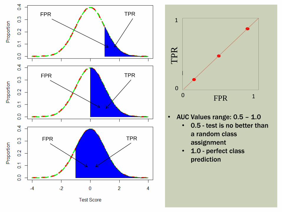
Depict tradeoffs between sensitivity and specificity over a range of cutoff values. In terms of disease:

Sensitivity (True positive rate [TPR]): identification of those who truly have the disease (D+) as having the disease (T+)

Specificity (True negative rate [TNR]): identification of those that do not actually have the disease (D-) as not having the disease (T-)

The value [1-Specificity] (False positive rate [FPR]) is used in graphs

Ideal classification models have high TPR while maintaining low FPR

TPR and FPR increase/decrease together

D- D+

c0

T- T+

TPR

FPR

0

FPR0

1

1

TP

R

c0

T+T-

D+D-

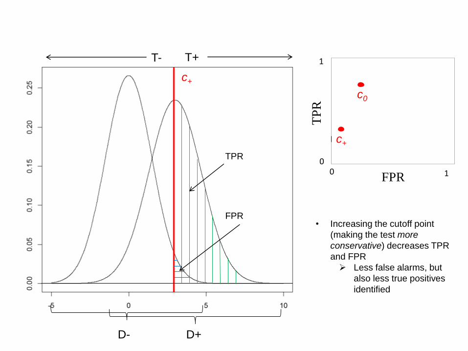
c+

TPR

FPR• Increasing the cutoff point

(making the test more

conservative) decreases TPR

and FPR

Less false alarms, but

also less true positives

identified

0

FPR0

1

1

TP

R

c+

c0

T+T-

D+D-

T+T-

c0

TPR

FPR

0

FPR0

1

1

TP

R

c+

c0

D+D-

0

FPR0

1

1

TP

R

c+

c0

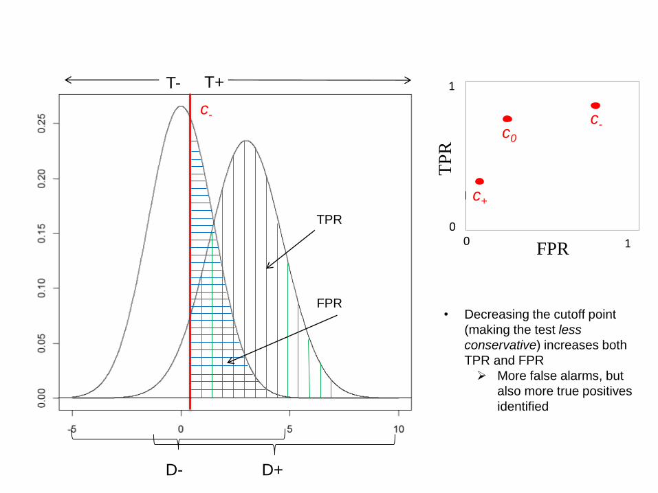
• Decreasing the cutoff point

(making the test less

conservative) increases both

TPR and FPR

More false alarms, but

also more true positives

identified

T+T-

c- c-

TPR

FPR

0FPR0

1

1

TP

R

0

FPR0

1

1

TP

R

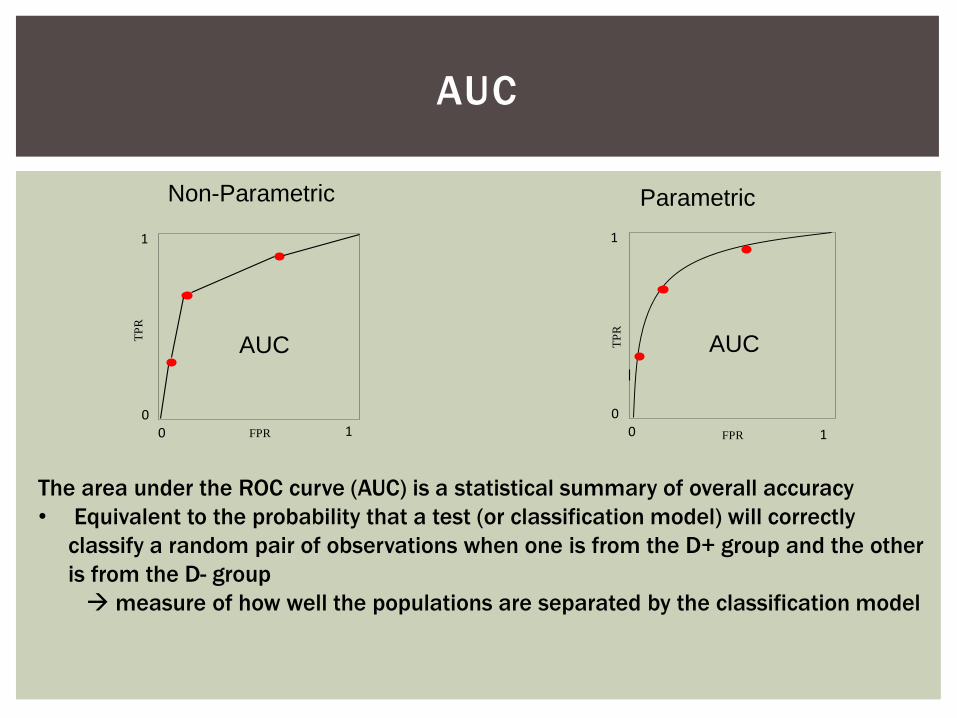
Non-Parametric Parametric

AUC AUC

The area under the ROC curve (AUC) is a statistical summary of overall accuracy

• Equivalent to the probability that a test (or classification model) will correctly

classify a random pair of observations when one is from the D+ group and the other

is from the D- group

measure of how well the populations are separated by the classification model

AUC

0

FPR0

1

1

TP

R

TPRFPR

TPRFPR

TPRFPR

• AUC Values range: 0.5 – 1.0

• 0.5 - test is no better than

a random class

assignment

• 1.0 - perfect class

prediction

PARAMETRIC CALCULATION

(NORMAL DISTRIBUTION)

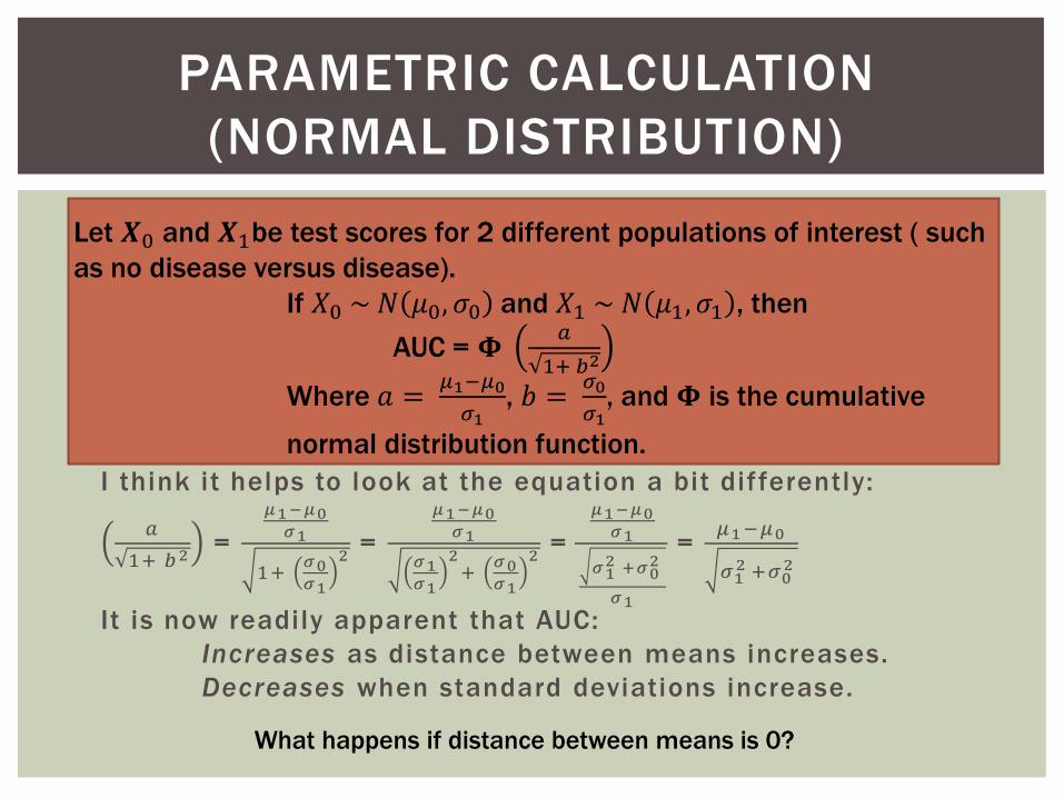
Let 𝑿0 and 𝑿1be test scores for 2 different populations of interest ( such

as no disease versus disease).

If 𝑋0 ~𝑁 𝜇0, 𝜎0 and 𝑋1 ~ 𝑁 𝜇1, 𝜎1 , then

AUC = 𝚽𝑎

1+ 𝑏2

Where 𝑎 =𝜇1−𝜇0

𝜎1, 𝑏 =

𝜎0

𝜎1, and 𝚽 is the cumulative

normal distribution function.

I think it helps to look at the equation a bit differently:

𝑎

1+ 𝑏2=

𝜇1−𝜇0𝜎1

1+𝜎0𝜎1

2=

𝜇1−𝜇0𝜎1

𝜎1𝜎1

2+

𝜎0𝜎1

2=

𝜇1−𝜇0𝜎1

𝜎12 +𝜎0

2

𝜎1

= 𝜇1−𝜇0

𝜎12 +𝜎0

2

It is now readily apparent that AUC:

Increases as distance between means increases.

Decreases when standard deviations increase.

What happens if distance between means is 0?

“DATA -BASED” NON -PARAMETRIC

ROC CURVE

FPR TPR

0 0.1

0 0.2

0 0.3

0 0.4

0.1 0.4

Group Score

1 10

1 9.4

1 9.2

1 7.6

0 7.4

1 7.3

0 7.1

1 6.5

0 6.3

0 6.2

0 5.6

1 5.4

0 5.3

1 4.7

1 4.6

0 4.2

1 4.1

0 3.9

0 1.8

0 1.5

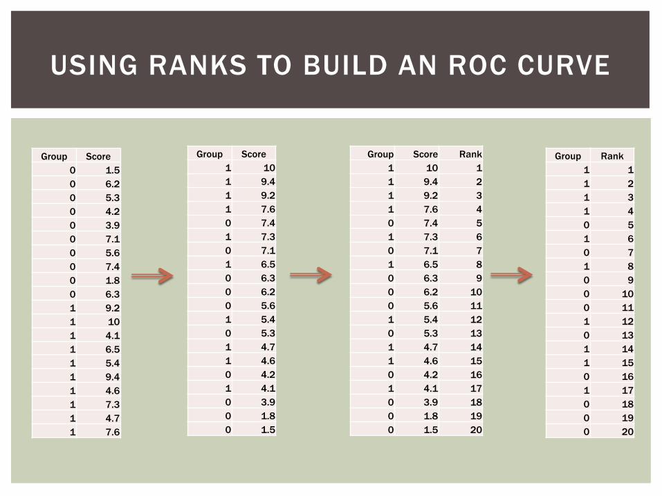
Sort data by score.

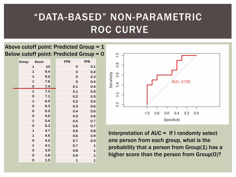
Above cutoff point: Predicted Group = 1

Below cutoff point: Predicted Group = 0

TP

FN

FN

FN

TN

FN

TN

FN

TN

TN

TN

FN

TN

FN

FN

TN

FN

TN

TN

TN

FPR TPR

0 0.1

Group Score

1 10

1 9.4

1 9.2

1 7.6

0 7.4

1 7.3

0 7.1

1 6.5

0 6.3

0 6.2

0 5.6

1 5.4

0 5.3

1 4.7

1 4.6

0 4.2

1 4.1

0 3.9

0 1.8

0 1.5

TP

TP

TP

TP

FP

FN

TN

FN

TN

TN

TN

FN

TN

FN

FN

TN

FN

TN

TN

TN

“DATA -BASED” NON -PARAMETRIC

ROC CURVE

FPR TPR

0 0.1

0 0.2

0 0.3

0 0.4

0.1 0.4

Group Score

1 10

1 9.4

1 9.2

1 7.6

0 7.4

1 7.3

0 7.1

1 6.5

0 6.3

0 6.2

0 5.6

1 5.4

0 5.3

1 4.7

1 4.6

0 4.2

1 4.1

0 3.9

0 1.8

0 1.5

0.1 0.5

0.2 0.5

0.2 0.6

0.3 0.6

0.4 0.6

0.5 0.6

0.5 0.7

0.6 0.7

0.6 0.8

0.6 0.9

0.7 0.9

0.7 1

0.8 1

0.9 1

1 1

Above cutoff point: Predicted Group = 1

Below cutoff point: Predicted Group = 0

Interpretation of AUC = If I randomly select

one person from each group, what is the

probability that a person from Group(1) has a

higher score than the person from Group(0)?

Group Score

0 1.5

0 6.2

0 5.3

0 4.2

0 3.9

0 7.1

0 5.6

0 7.4

0 1.8

0 6.3

1 9.2

1 10

1 4.1

1 6.5

1 5.4

1 9.4

1 4.6

1 7.3

1 4.7

1 7.6

USING RANKS TO BUILD AN ROC CURVE

Group Score Rank

1 10 1

1 9.4 2

1 9.2 3

1 7.6 4

0 7.4 5

1 7.3 6

0 7.1 7

1 6.5 8

0 6.3 9

0 6.2 10

0 5.6 11

1 5.4 12

0 5.3 13

1 4.7 14

1 4.6 15

0 4.2 16

1 4.1 17

0 3.9 18

0 1.8 19

0 1.5 20

Group Score

1 10

1 9.4

1 9.2

1 7.6

0 7.4

1 7.3

0 7.1

1 6.5

0 6.3

0 6.2

0 5.6

1 5.4

0 5.3

1 4.7

1 4.6

0 4.2

1 4.1

0 3.9

0 1.8

0 1.5

Group Rank

1 1

1 2

1 3

1 4

0 5

1 6

0 7

1 8

0 9

0 10

0 11

1 12

0 13

1 14

1 15

0 16

1 17

0 18

0 19

0 20

“RANK -BASED” NON-PARAMETRIC ROC

CURVE

Group Rank

1 1

1 2

1 3

1 4

0 5

1 6

0 7

1 8

0 9

0 10

0 11

1 12

0 13

1 14

1 15

0 16

1 17

0 18

0 19

0 20

1 - Specificity Sensitivity

0 0.1

0 0.2

0 0.3

0 0.4

0.1 0.4

0.1 0.5

0.2 0.5

0.2 0.6

0.3 0.6

0.4 0.6

0.5 0.6

0.5 0.7

0.6 0.7

0.6 0.8

0.6 0.9

0.7 0.9

0.7 1

0.8 1

0.9 1

1 1

Above cutoff point: Predicted Group = 1

Below cutoff point: Predicted Group = 0

Interpretation of AUC = If I randomly select

one person from each group, what is the

probability that a person from Group(1) is

ranked higher than the person from Group(0)?

RANK-BASED VS SCORE-BASED NON-

PARAMETRIC ROC CURVE

Curves are identical

Non-parametric (or “data–based” or “Empirical”) curves are inherently rank-based

“Rankiness” nice statistical properties without the need to assume a

particular distribution

N0N-PARAMETRIC CALCULATION

Let 𝑿0 and 𝑿1be test scores OR ranks based on scores for 2 different

populations of interest (such as no disease versus disease).

If there is no distributional assumption for the values of 𝑿0 and 𝑿1, then

AUC = 1

𝑛0𝑛1 𝑖=1𝑛1 𝑗=1

𝑛2 𝐼(𝑋𝑖1, 𝑋𝑗0)

where 𝐼(𝑋𝑖1, 𝑋𝑗0) =

1 𝑖𝑓 𝑋𝑖1 > 𝑋𝑗0 1 2 𝑖𝑓 𝑋𝑖1 = 𝑋𝑗00 𝑖𝑓 𝑋𝑖1 < 𝑋𝑗0

AUC is equal to the Mann-Whitney U statistic; it compares the sums of ranks.

- Approximately normally distributed for large samples.

- Robust (not sensitive to outliers)

Introduction

Parametric ROC Curve

Non-Parametric ROC Curve

Examples

Single Cutoff-Point: Single mutation

Continuous outcome: Gene expression levels

Discreet outcome: Gene ranks

Extensions

‘Non-Proper’ ROC Curves

Multi-class ROC Analysis

OUTLINE

EXAMPLE: SINGLE CUT-POINT,

SINGLE MUTATION

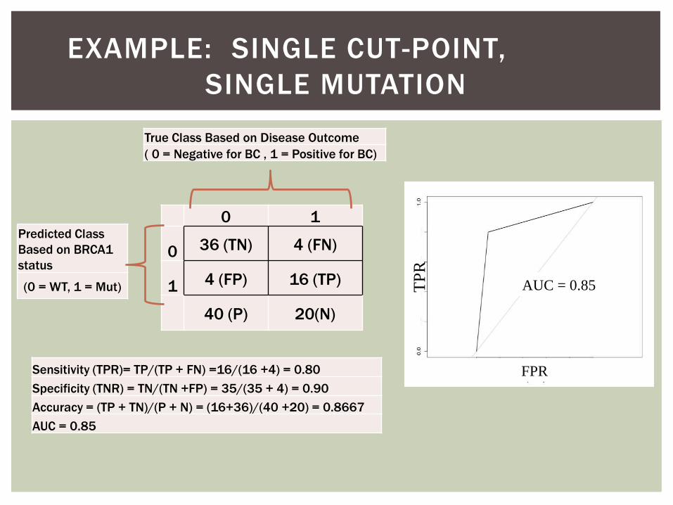
0 1

0 36 (TN) 4 (FN)

1 4 (FP) 16 (TP)

40 (P) 20(N)

Predicted Class

Based on BRCA1

status

(0 = WT, 1 = Mut)

True Class Based on Disease Outcome

( 0 = Negative for BC , 1 = Positive for BC)

Sensitivity (TPR)= TP/(TP + FN) =16/(16 +4) = 0.80

Specificity (TNR) = TN/(TN +FP) = 35/(35 + 4) = 0.90

Accuracy = (TP + TN)/(P + N) = (16+36)/(40 +20) = 0.8667

AUC = 0.85

FPR

TP

R

AUC = 0.85

A CLOSER LOOK AT AUC

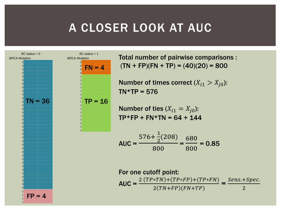
BC status = 0 BC status = 1

BRCA Mutation BRCA Mutation

0 0

0 0

0 0

0 0

0 1

0 1

0 1

0 1

0 1

0 1

0 1

0 1

0 1

0 1

0 1

0 1

0 1

0 1

0 1

0 1

0

0

0

0

0

0

0

0

0

0

0

0

0

0

0

0

1

1

1

1

TN = 36

FP = 4

TP = 16

FN = 4

Total number of pairwise comparisons :

(TN + FP)(FN + TP) = (40)(20) = 800

Number of times correct (𝑋𝑖1 > 𝑋𝑗0):

TN*TP = 576

Number of ties (𝑋𝑖1 = 𝑋𝑗0):

TP*FP + FN*TN = 64 + 144

AUC = 576+

1

2(208)

800= 680

800= 0.85

For one cutoff point:

AUC = 2 𝑇𝑃∗𝑇𝑁 + 𝑇𝑃∗𝐹𝑃 +(𝑇𝑃∗𝐹𝑁)

2 𝑇𝑁+𝐹𝑃 (𝐹𝑁+𝑇𝑃)= 𝑆𝑒𝑛𝑠.+𝑆𝑝𝑒𝑐.

2

A GEOMETRIC LOOK AT AUC

FPR

TP

R

.5(0.1*0.8 )= 0.04

.5(1+0.8)*0.9 = 0.81

AUC via Trapezoidal Integration: 0.81 + 0.04 = 0.85

*ROC analysis is not typically performed for single cutoff scenarios but hopefully this

sheds light on the probabilistic/geometric nature of AUC

Introduction

Parametric ROC Curve

Non-Parametric ROC Curve

Examples

Single Cutoff-Point: Single mutation

Continuous outcome: Gene expression levels

Discreet outcome: Gene ranks

Extensions

‘Non-Proper’ ROC Curves

Multi-class ROC Analysis

OUTLINE

Hypothetical situation:

I read about an cell-line experiment that found certain genes upregulated in MCF-7 (breast cancer) cells. I want to see how the results translate to human BC tumors.

I choose two genes and go to the Genomics Portals website to obtain gene expression data

Dataset: Breast invasive carcinoma from TCGA

Pubmed source: TCGA_BRCA_exp_HiSeqV2

Genes:

IFI27 (interferon, alpha-inducible protein 27) – promotes cell death and is associated with healing

FN1 (fibronectin 1) - cell adhesion and migration processes

How well do the corresponding gene expression levels discriminate tumor samples from normal tissue samples?

EXAMPLE: CONTINUOUS OUTCOME -

GENE EXPRESSION LEVELS

EXAMPLE: CONTINUOUS OUTCOME -

GENE EXPRESSION LEVELS

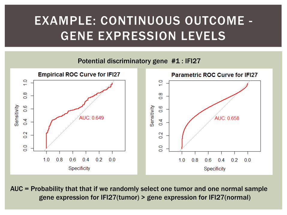
Potential discriminatory gene #1 : IFI27

AUC = Probability that that if we randomly select one tumor and one normal sample

gene expression for IFI27(tumor) > gene expression for IFI27(normal)

EXAMPLE: CONTINUOUS OUTCOME -

GENE EXPRESSION LEVELS

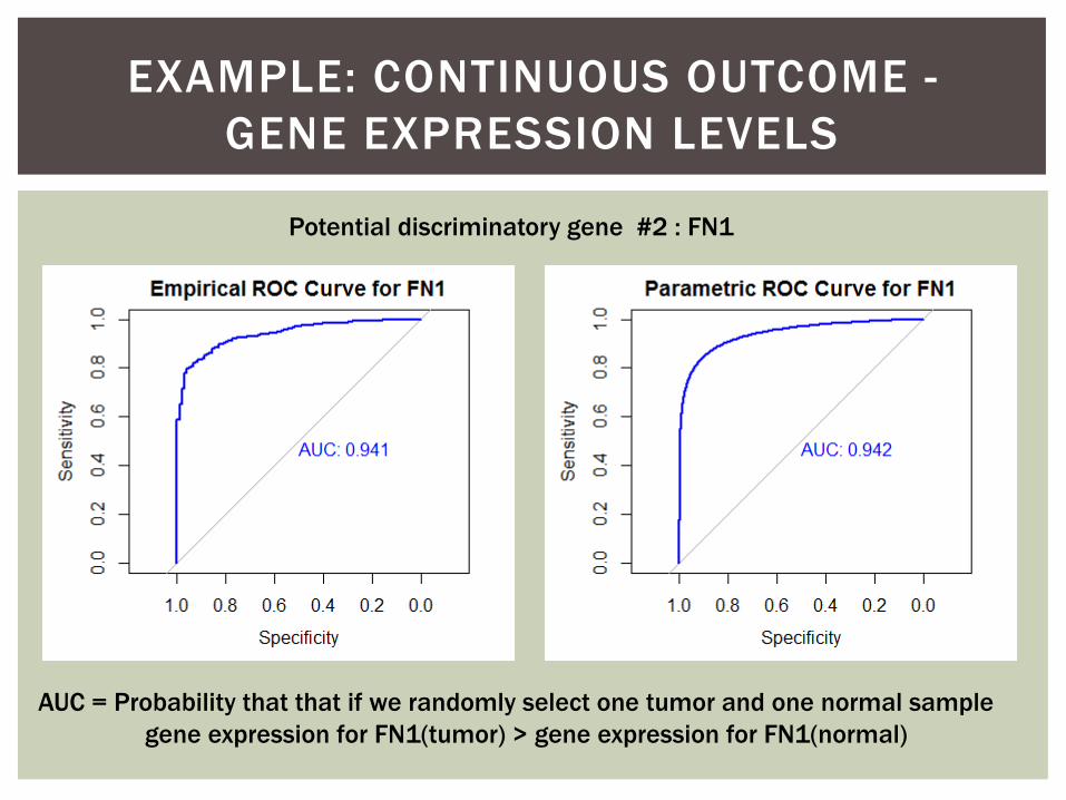
Potential discriminatory gene #2 : FN1

AUC = Probability that that if we randomly select one tumor and one normal sample

gene expression for FN1(tumor) > gene expression for FN1(normal)

EXAMPLE: CONTINUOUS OUTCOME -

GENE EXPRESSION LEVELS

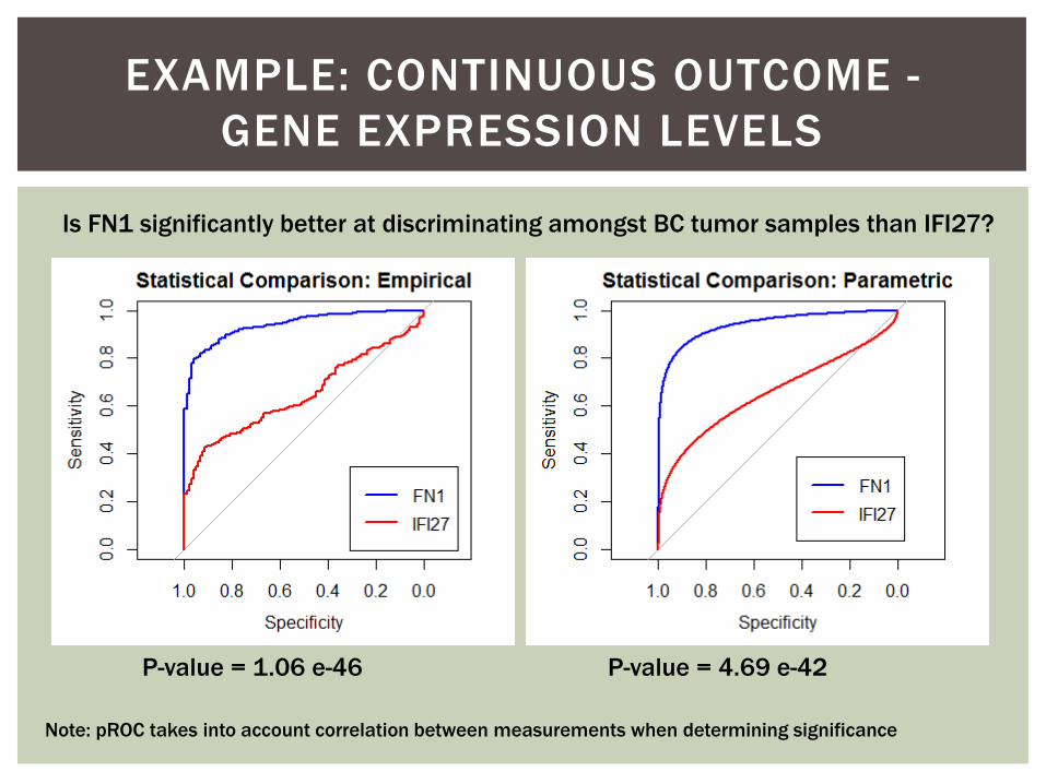
Is FN1 significantly better at discriminating amongst BC tumor samples than IFI27?

Note: pROC takes into account correlation between measurements when determining significance

P-value = 1.06 e-46 P-value = 4.69 e-42

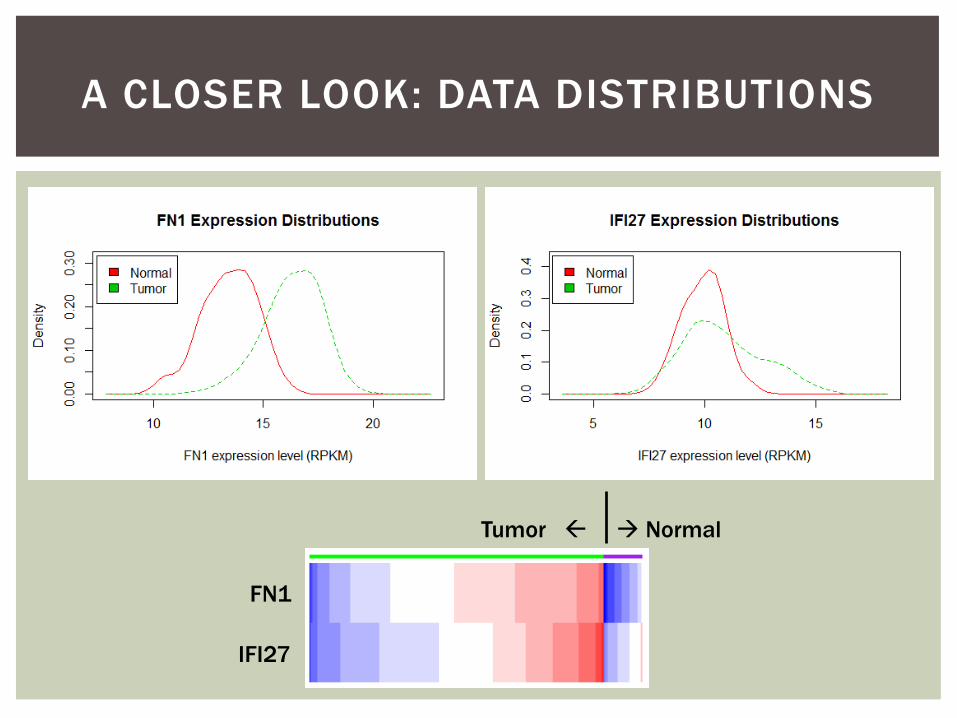
A CLOSER LOOK: DATA DISTRIBUTIONS

Tumor Normal

FN1

IFI27

EXAMPLE: CONTINUOUS OUTCOME -

GENE EXPRESSION LEVELS

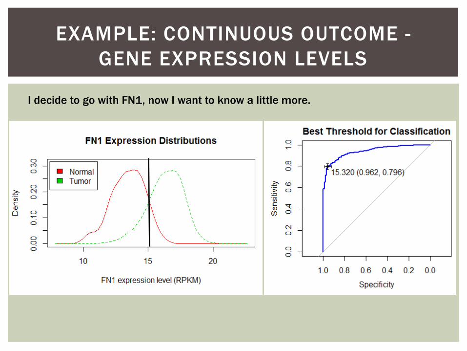
I decide to go with FN1, now I want to know a little more.

Introduction

Parametric ROC Curve

Non-Parametric ROC Curve

Examples

Single Cutoff-Point: Single mutation

Continuous outcome: Gene expression levels

Discreet outcome: Gene ranks

Extensions

‘Non-Proper’ ROC Curves

Multi-class ROC Analysis

OUTLINE

Hypothetical situation:

I have been using DEseq for dif ferential expression analysis. I

want to start using edgeR, but I hear it is less conservative

than DEseq.

Since edgeR is less conservative, I am concerned that it will return

more false positives than DEseq.

On the other hand, I am concerned that DEseq will return less true

positives than edgeR.

I construct a simulation data set to represent two groups and

expression levels for 50 genes.

I choose at random 20 genes to be up- or down-regulated (DE) between

groups when I simulate the data

(for more detail see Soneson & Delorenzi 2013)

I run DE on DEseq and edgeR and then rank the genes by p-value.

EXAMPLE: DISCREET OUTCOME -

RANKING OF DE GENES

EXAMPLE: DISCREET OUTCOME

DATA SET-UP

GeneID DEstatus rankedgeR rankDEseq

gene1 1 1 1

gene2 1 2 2

gene3 1 3 3

gene4 1 4 4

gene5 1 5 5

gene6 1 6 6

gene7 1 8 7

gene8 1 9 8

gene9 1 11 9

gene10 1 13 10

gene11 1 14 11

gene12 1 15 12

gene13 1 17 14

gene14 1 20 15

. . . .

. . . .

. . . .

gene37 0 37 35

gene38 0 38 36

gene39 0 39 37

gene40 0 40 39

gene41 0 41 40

gene42 0 42 41

gene43 0 43 42

gene44 0 44 43

gene45 0 45 44

gene46 0 46 46

gene47 0 47 47

gene48 0 48 48

gene49 0 49 49

gene50 0 50 50

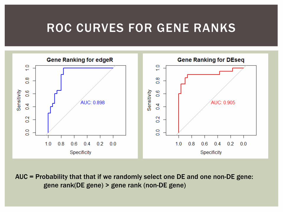
ROC CURVES FOR GENE RANKS

AUC = Probability that that if we randomly select one DE and one non-DE gene:

gene rank(DE gene) > gene rank (non-DE gene)

DIFFERENCES IN PERFORMANCE

Is there another way to identify differences in performance?

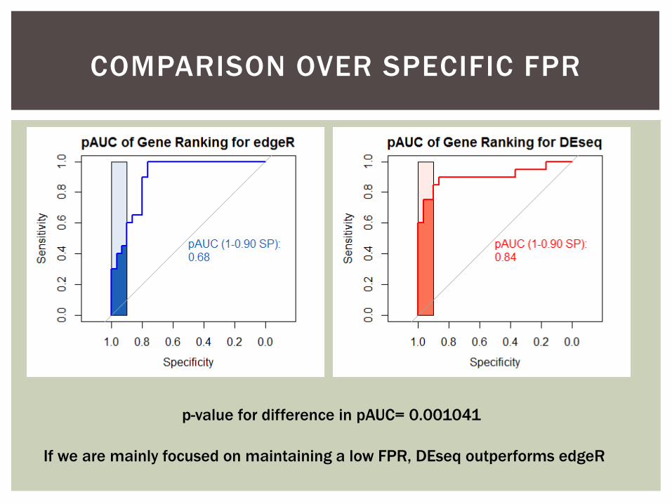
COMPARISON OVER SPECIFIC FPR

p-value for difference in pAUC= 0.001041

If we are mainly focused on maintaining a low FPR, DEseq outperforms edgeR

COMPARISON OVER SPECIFIC TPR

p-value for difference in pAUC= 0.03188

If we want to identify as many genes as possible, edgeR outperforms DEseq at a

lower threshold

Introduction

Parametric ROC Curve

Non-Parametric ROC Curve

Examples

Single Cutoff-Point: Single mutation

Continuous outcome: Gene expression levels

Discreet outcome: Gene ranks

Extensions

‘Non-Proper’ ROC Curves

Multi-class ROC Analysis

OUTLINE

SCENARIOS FOR ‘NOT-PROPER’ ROC

CURVES

Parodi et al. BMC Bioinformatics 2008

9:410 doi:10.1186/1471-2105-9-410

SIMPLIFIED SCENARIO: SAME MEAN,

DIFFERENT SD’S

𝐴𝑈𝐶 = 𝚽𝜇1−𝜇0

𝜎12+𝜎0

2

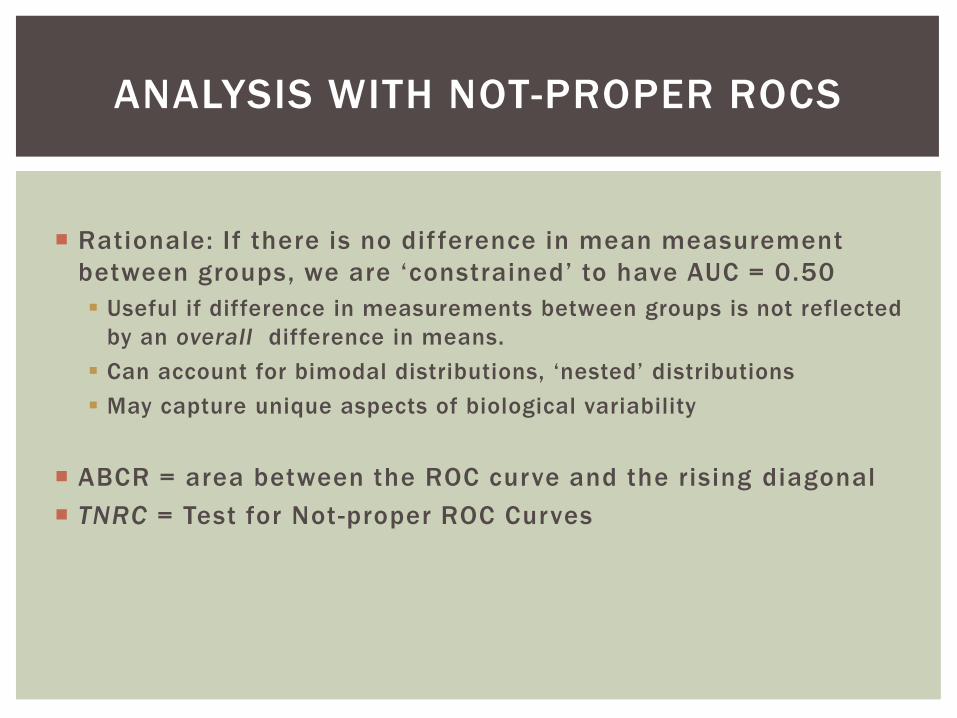
Rationale: If there is no dif ference in mean measurement

between groups, we are ‘constrained’ to have AUC = 0.50

Useful if difference in measurements between groups is not reflected

by an overall difference in means.

Can account for bimodal distributions, ‘nested’ distributions

May capture unique aspects of biological variability

ABCR = area between the ROC curve and the rising diagonal

TNRC = Test for Not-proper ROC Curves

ANALYSIS WITH NOT-PROPER ROCS

Introduction

Parametric ROC Curve

Non-Parametric ROC Curve

Examples

Single Cutoff-Point: Single mutation

Continuous outcome: Gene expression levels

Discreet outcome: Gene ranks

Extensions

‘Non-Proper’ ROC Curves

Multi-class ROC Analysis

OUTLINE

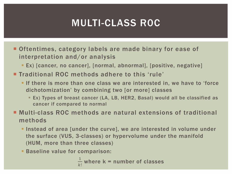
Oftentimes, category labels are made binary for ease of

interpretation and/or analysis

Ex) [cancer, no cancer], [normal, abnormal], [positive, negative]

Traditional ROC methods adhere to this ‘rule’

If there is more than one class we are interested in, we have to ‘force

dichotomization’ by combining two [or more] classes

Ex) Types of breast cancer (LA, LB, HER2, Basal) would all be classified as

cancer if compared to normal

Multi-class ROC methods are natural extensions of traditional

methods

Instead of area [under the curve], we are interested in volume under

the surface (VUS, 3-classes) or hypervolume under the manifold

(HUM, more than three classes)

Baseline value for comparison:

1

𝑘!where k = number of classes

MULTI-CLASS R0C

Class 1 Class 2 Class 3

c1 c2

T1 T2 T3

TCR1

Instead of TPR and

FPR, we are

concerned with the

three true

classification rates

(TCR) for any two

cutoff points (c1, c2),

where c1 < c2

TCR2

TCR3

VOLUME UNDER THE SURFACE

Each possible pair of cutoff points yields a triplet of

true classification rates

Triplet is coordinates for point in 3-D space

Points are plotted and connected to form an ROC surface

Volume under the ROC surface (VUS) is analogous to AUC

VUS of 1

6(≈ 0.167) indicative of random class assignment

Non-Parametric (Nakas & Yiannoutsos 2004) Parametric (Kang & Tian 2013)

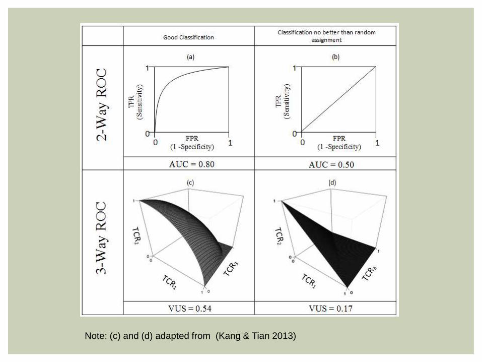
Note: (c) and (d) adapted from (Kang & Tian 2013)

EXAMPLE: MICROSATELLITE INSTABILITY

IN COLON CANCER

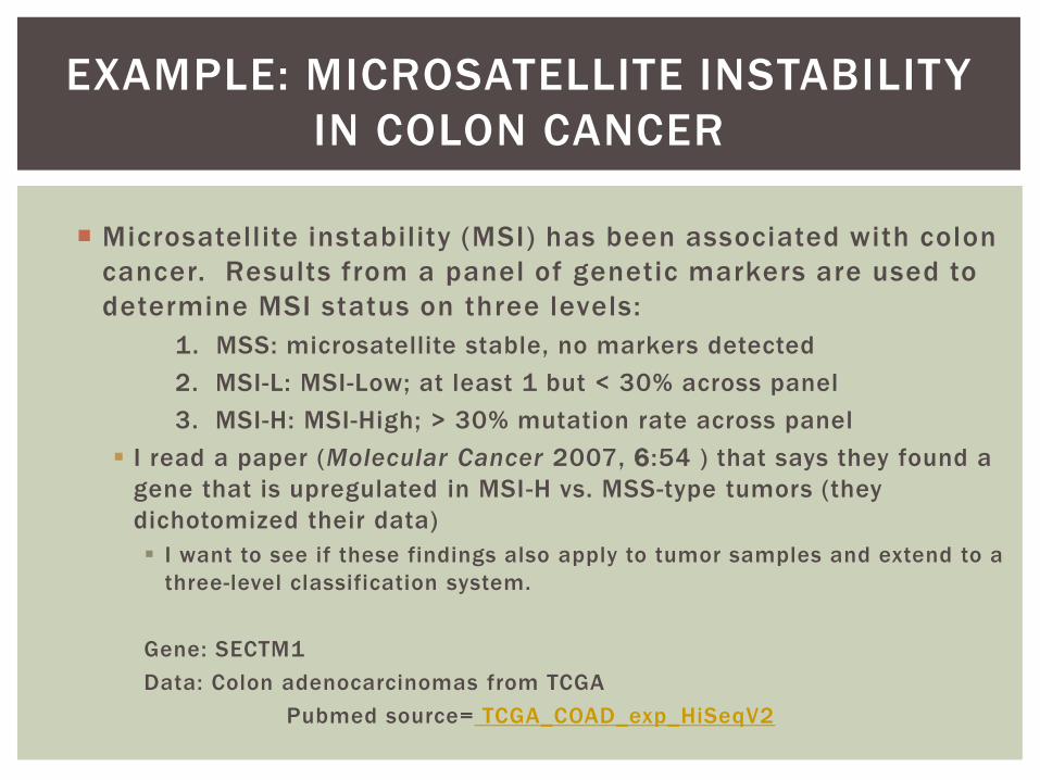
Microsatellite instability (MSI) has been associated with colon

cancer. Results from a panel of genetic markers are used to

determine MSI status on three levels:

1. MSS: microsatellite stable, no markers detected

2. MSI-L: MSI-Low; at least 1 but < 30% across panel

3. MSI-H: MSI-High; > 30% mutation rate across panel

I read a paper (Molecular Cancer 2007, 6:54 ) that says they found a

gene that is upregulated in MSI-H vs. MSS-type tumors (they

dichotomized their data)

I want to see if these findings also apply to tumor samples and extend to a

three-level classification system.

Gene: SECTM1

Data: Colon adenocarcinomas from TCGA

Pubmed source= TCGA_COAD_exp_HiSeqV2

EXAMPLE: MICROSATELLITE INSTABILITY

IN COLON CANCER

[Edited] Raw Data Summary:

n mu sd

Level 1: MSS 98 8.21 1.17

Level 2: MSI-L 25 8.03 1.29

Level 3: MSI-H 25 10.05 1.49

VUS=0.3419, 95% CI=[0.2258, 0.457]

Best cut-points: lower(c1)=8.0439, upper(c2)=9.3773

The group correct classification probabilities are

MSS MSH-L MSH-H

0.4184 0.6429 0.8000

VUS = Probability that if we choose at random one MSS, MSI-L and MSI-H sample:

SECTM1MSS < SECTM1MSI-L < SECTM1MSI-H

EXAMPLE: MICROSATELLITE INSTABILITY

IN COLON CANCER

[Edited] Raw Data Summary:

n mu sd

Level 1: MSI-L 25 8.03 1.29

Level 2: MSS 98 8.21 1.17

Level 3: MSI-H 25 10.05 1.49

VUS(new)=0.4692, 95% CI=[0.3289, 0.6017]

VUS(old)=0.3419

Best cut-points: lower(c1)=7.4214, upper(c2)=9.3773

The group correct classification probabilities are

MSS MSH-L MSH-H

0.4184 0.4400 0.8000

VUS = Probability that if we choose at random one MSS, MSI-L and MSI-H sample:

SECTM1MSI-L < SECTM1MSS < SECTM1MSI-H

SOMETHING TO CONSIDER:

REMEMBER IFI27?

The original AUC was not very impressive, but levels are moderately higher in tumors

Brief literature review yields info that IFI27 upregulation has been implicated in epithelial cancer cells.

Can we gain further insight if we stratify by cell type?

We can’t do this with the TCGA data, but Genomics Portal has a different data set I can use

Tumor and normal tissue samples classified as either epithelial or squamous

PubMed source= GSE10797,

Heterogeneity of BC

adds ‘noise’ to the ROC

analysis

Keeping in mind small

sample size, a few

sources in this case

include:

Higher levels of IFI27

measured in normal

stromal cells

An ‘island’ of cancerous

epithelial cells with

marked IFI27

upregulation

SOMETHING TO CONSIDER:

REMEMBER IFI27?

Flexible tool for evaluating classification models

Provides statistical and graphical measures of overall accuracy

Yields optimal cutoff values for prediction

Some considerations for use in functional genomics:

Heterogeneity of biological data

We are using relatively simple methods but dealing with appreciably

complex phenomena

Unequal sample sizes for groups

Generally more cancer samples than normal samples

More genes are non-DE vs DE (when considering ranking systems)

This is only the tip of the iceberg!

Bayesian methods, semi-parametric methods, misclassification costs,

training/validation issues, multivariable models…

SUMMARY OF ROC ANALYSIS

QUESTIONS?

http://stats.stackexchange.com/questions/423/what-is-your-favorite-data-analysis-cartoon?page=2&tab=votes#tab-top