Dr Abraham T Mathew

Introduction to Robust Control

What is a Control System?

Is it the physical system?

Is it the mathematical system?

CONTROL SYSTEM OUTPUT

INPUT

INPUT

INPUT

SYSTEM BOUNDARY

ENVIRONMENT

SUCCESS IN CONTROL DESIGN IS SAID TO BE BASED ON THE SUCCESS IN IDENTIFYING THE SYSTEM BOUNDARY,

INPUTS,OUTPUTS & THE ENVIRONMENT

Model Based Control Design- Issues Analytical or computational models cannot truly characterize and

emulate the phenomenon.

A model, no matter how detailed, is never a completely accurate representation of a real physical system

Control Design-classical way

Normally, in the conventional control design for SISO system, the stability margin is specified to ensure stability in the presence of model uncertainties

But, the uncertainties or perturbations are not quantified, nor performance was not taken into account in terms of disturbance, noise etc.

For MIMO systems, many of the SISO methods cannot be scaled up

Robust Control

Design a controller such that-

some level of performance of the controlled system is guaranteed-

irrespective of the changes in the plant dynamics/process dynamics within a predefined class and

the stability is guaranteed

Control design targets Stability

Disturbance rejection

Sensor(measurement) noise rejection

Avoidance of actuator saturation

Robustness- the process/plant performance should not deteriorate to unacceptable level if there occurs the changes due to the uncertainties

All these targets cannot be achieved simultaneously and perfectly. So there has to be some compromise or tradeoffs, because of various reasons

Modeling in the context of robust control

We consider a simple example !!

Modeling a DC Servo We consider a DC servo mechanism consisting of a DC

motor, gear train, and the load shaft

It is required to control the angular displacement and speed using a voltage signal applied across the armature

Motor

Load

Linear Model of the DC Servo-Physical

Equations of dynamics

L

e

a

a

a

a

m

e

m TJ

tv

Li

L

R

L

NK

J

NKL

i

0

10

)(10

0

0

00

010

i

010

001

TF FORM

21

2

0

222)(

)(

bsbss

a

LJ

KNs

L

Rss

LJ

NK

sv

s

ae

m

a

a

ae

m

Nominal Model Km=0.05 Nm/A, Ra=1.2 ohms, La=0.05H

Jm=8x10-4 kgm2 , J=0.020 kgm2

N=12

Je=J+N2Jm=0.1352 kgm2

Uncertainty Let the parameters are subject to changes as follows

0.04≤Km ≤0.06

6x10-4 ≤Jm ≤ 10-3

0.01≤J ≤0.05

Model with Uncertainty

(as an Interval System)

53.4] ,8.47[12ss

99.58] ,22.74[)(

2

ssG

Abstracting a Control System Structure

Control System Structure

Disturbance w(t)

Plant/Process

P Sensor

S Controller

C

Sensor

S1

y u

wm Noise v(t)

Output ym Input yd

System Equations If the Plant is LTI the zero state linearity dictates that y is a linear

combination of effects of the two plant inputs u and w That is

Quite often it is convenient to work with the disturbance d(s) at the

plant output given as

Then, we have

(1) )()()()()( swsPsusPsyw

(2) )()()( swsPsdw

(3) )()()()( sdsusPsy

System Equations Sensor is assumed to have two inputs, plant output y and the

measurement noise v. So, we have

Ideally Ps(s)=1 and v(t)=0 so that ym=y

(this is achieved if sensor bandwidth is larger than system bandwidth or we say the sensor is fast and accurate)

(4) )()()()( svsysPsysm

Now, look at the Controller

Disturbance w(t)

Plant/Process

P Sensor

S Controller

C

Sensor

S1

ym y u yd

wm Noise v(t)

Contd… Controller gets three inputs ym, yd and wm

Here wm is the disturbance measured using suitable sensor

Let the controller be LTI. Then

Not all the three inputs need to be used always here. Several control structures are defined according to whether ym, yd or wm is used to produce u or not . Accordingly we will have different schemes of control

(5) )()()()()()()( swsFsysFsysFsumwmmdd

1. Single Degree of Freedom controller

When Fm=-Fd and Fw=0, we have

The figure shows 1DoF Control Structure realizing this equation

)]()()[()( sysysFsumdd

Fd

ym

yd

- +

u

Two Degree of Freedom Controller

If we have a structure of the form given below, designer will have freedom to independently select Fm and Fd we will have the TDoF Feedback Controller structure

Fm ym

yd

+ +

u Fd

Feedback Control Scheme

P Ps Fd

Fm

+ yd

Pw

Fw

v w

ym + +

+ +

+

+ u

d

y

Problem formulation System enclosed in the dotted box is seen to have three

inputs and one output

By assuming linearity, we can say that plant output y(t) is produced as a superposition of the effects of these three signals coming to the output port through three transfer channels

That is

)()()()()()()( svsHswsHsysHsy

vwdd

Tracking problem Let the error e(t) be defined as e(t)=yd-y

That is,

The central design problem is to obtain Hd, Hw, and Hv with desirable properties using appropriate methods or criteria

)()()()()()(1)(

)()()()()()()()(

svsHswsHsysHse

Or

svsHswsHsysHsyse

vwdd

vwddd

Look at it again

P Ps Fd

Fm

+ yd

Pw

Fw

v w

ym + +

+ +

+

+ u

d

y

Emphasis for output disturbance In cases where it is desirable or convenient to work with the

output disturbance d rather than w, we have

)()()()()()()( svsHsdsHsysHsyvwddd

)()()()()()(1)(

)()()()()()()()(

svsHsdsHsysHse

Or

svsHsdsHsysHsyse

vwddd

vwdddd

Tracking performance For the system to ideally track the reference, the error must

be zero To achieve this for all possible yd,v,w and d, we would

require Hd(s)=1 and Hw(s)= Hwd(s)=Hv(s)=0 In the practical setting, as we see more in detail, we can see

that this condition cannot be satisfied perfectly for the entire bandwidth or entire region of system perturbations

Some design tradeoffs, optimality conditions and so on would have to be called for as we have already noted.

Admissible/acceptable designs In order to do the adjustment/tradeoff for obtaining an

admissible or acceptable design and discriminate between acceptable and unacceptable departures from the ideal performance, we need to have the specifications

These specifications give rise to different control structures like open loop, feedforward, feedback, etc.

We may differentiate between SISO and MIMO and start with SISO and generalize the notations for MIMO, subsequently

Control System Performance From a system’s perspective, the performance specification

for control system starts with “Stability” Followed by Sensitivity, Disturbance Rejection, Noise

Rejection etc. where needed.

Stability When it comes to stability, in the modern settings of design,

we consider two classes of stability, namely Input-output stability

Internal stability

Internal stability is of paramount importance in the MIMO system framework, both in Matrix Transfer function form and State variable/transfer function forms

Internal Stability A system to be internally stable means all the transfer functions

associated with all the transfer channels connecting exogenous input to the output(including set point, disturbance & noise) shall be stable

In reality, it is possible for a system to be internally unstable and yet to have a stable “set point to output” channel transfer functions

Under this circumstance, we say that system has unstable hidden modes

Therefore, internal stability must be ensured before the transfer function that define the response to the system inputs are considered

Design Model

Let P be a set of all plants that each member of set P is an admissible model, given the uncertainty region (interval)

P0 in P is one model with the nominal value of the parameters

If P0 is used for the robust designs, then let us call P0 as Design

model (for the sake of convenience!!)

Model Uncertainty & Internal stability

If the plant is expected to deviate from the design model(nominal model), it is better represented by a set of models centered on the design model(nominal model)

For a control system to be acceptable, the design must be internally stable for every model in the set

This property is known as robust stability

Once stability & robustness are assured, we can shift the attention to “response”

Summary A model of the physical system is only an approximation of

the real phenomenon/process

Control system output is the measurement showing the status or effectiveness of control

Inputs, in a general framework will include set point, disturbance and measurement noise

Summary contd… Models are subjected to various uncertainties

Nominal model in the set of uncertain models can be used as Design model

Internal Stability and robust stability are starting points for good control system design

Once stability is assured, other performance measures can be specified

Design Dilemma It will not usually be possible(which we will see in detail) to

have good set point tracking, and disturbance rejection and noise rejection uniformly effectively for all functions of yd, v, w and d

Also, emphasis on sensitivity on one may negatively affect the other

Robust Control System A system is said to be robust when

It is durable, hardy and resilient

It has low sensitivities in the system passband

It is stable over the range of parameter variations

The performance continues to meet the specifications in the presence of a set of changes in the system parameters

Robustness is the sensitivity to the effects that are not

considered in the analysis and design-

for example,

the disturbances,

measurement noise, and

unmodeled dynamics

Sensitivity & Sensitivity Analysis

Sensitivity It is the percentage change in system transmission or

response or some quantity of interest with respect to the percentage change in another quantity

In control theory we use Parameter Sensitivity

System Sensitivity

Root Sensitivity

Eigenvalue Sensitivity

Parameter Sensitivity Let T be the system function which depends on a parameter

Then, the parameter sensitivity ST of T with respect to s

defined as

TT

TT

TS

T

ln

ln

System Sensitivity Let T be the system closed loop transfer function which

depends on the open loop transfer function G

Then sensitivity of T w.r.t G is given as

GG

TT

GG

TT

G

TS

T

G

ln

ln

Root Sensitivity Let T be the system closed loop transfer function with the ith

root given as i and the parameter of interest is say K

Root sensitivity is the sensitivity in terms of the position of the roots of the characteristic equation on the (, j) plane(root locus plane)

Significance of Root Sensitivity Roots of the characteristic equation represents the

dominant(visible) modes of the transient response

The effect of parameter variation on the position of the root and the direction of shift of the root are important and useful measures to say about the sensitivity

Can be combined with Root Locus Method for Control Designs

Definition of Root Sensitivity

The root sensitivity of the system T(s) is defined as

Let

KKK

S ii

K

i

ln

)(

)()(

1

11

i

n

i

j

m

j

s

zsKsT

Contd… Let K be a parameter that influences the location of the roots i

and the gain K1

Then the root sensitivity is related to the system sensitivity to K and is given as(if zeros of T(s) are not dependent)

In the event of gain K1 independent of K, we have

n

i

i

iT

K

sKK

KS

1

1

)(

1

lnln

ln

n

i

i

K

n

i

i

iT

K

sS

sKS i

11 )(

1

)(

1

ln

Eigenvalue Sensitivity Let us assume that we have the relation(A is from the state

space equation)

Differentiating with respect to the element akj of A we will have

iiiA

kj

i

ii

kj

i

kj

i

i

kjaaa

Aa

A

Contd… Premultiplying with i , the left eigenvector we have ii=1

and i (A-i I)=0

Then, we get

kj

i

i

kj

i

aa

A

Contd… All elements in will be zero except the (k,j)th element,

which will be 1

Therefore we get

This is the eigenvalue sensitivity

kja

A

jiik

kj

i

a

Sensitivity Analysis of transfer

functions

Consider a closed loop system as shown in Figure

G yd

y u +

-

GG

T

T

G

GG

TT

G

TS

G

GT

T

G

1

1

ln

ln

1

Waterbed effect Now, add T and S

We get T+S =1

System with cascade compensator

We consider the following system

G yd y u +

-

K

GKG

T

T

G

GG

TT

G

TS

GK

GKT

T

G

1

1

ln

ln

1

Check T+S

System with feedback compensator

Consider the following system

G yd

y u +

-

H

GHG

T

T

G

GG

TT

G

TS

GH

GT

T

G

1

1

ln

ln

1

Check T+S

Sensitivity & Complimentary Sensitivity Functions

In the Robust Control Literature, Sensitivity Function plays a crucial role

Let S(s) be the Sensitivity Function

Then T(s) is the Complimentary Sensitivity Function such that S+T=1 for SISO and S+T=I for MIMO

Open Loop Control

Open Loop Control It is the simplest control structure

Limited in performance

Usually reserved for special applications where feedback control is either impossible or unnecessary

It is a good starting point for control design

It helps to appreciate the advantages of feedback control

Stability, performance etc are relatively in simpler forms to understand

Open Loop Structure

F P yd u y

d

+ +

-

+

e

Input-Output Relations In open loop control input yd is usually a synthesized signal

for the given application and u is derived from that as shown

Open loop control requires no measurements.

Now, from Figure above, we write as

dFPyyd

dyFPeandd )1(

1)(

)()()(

sHand

sPsFsH

wd

d

Tracking Performance Perfect tracking of yd occurs if

That is, if

The practical objective is to make

in the system passband

1)()()( sPsFsHd

1)()( sPsF

1)()( jPjF

Disturbance rejection Since open loop control does nothing to attenuate

the effects of disturbance inputs nor does it amplify them either

1)( sHwd

Sensitivity The sensitivity of with respect to P(s) is calculated as

follows

A sensitivity 1 implies that a given percent change in P translates into the equal percent change in the transmission function

Open loop control does not affect sensitivity

)(sHd

1

)(

0

0

00

PP

FPPF

S

PFFPPPFH

H

P

d

)( jHd

Stability Conditions We modify the block diagram of the Open loop control

system as shown here

F P yd u y

z

+

+

v

Analysis In any system, any addition or deletion of some of the input lines

or some output lines won’t alter the internal stability We shall add inputs and outputs and view this as injecting test

inputs into the system and taking extra measurements, neither of which is expected to change the stability properties of the system

The test inputs and and outputs are chosen so that the resulting system is controllable and observable

For such a fully controllable and observable system there shall not be any hidden modes

So, internal stability is then guaranteed by input-output stability

F P yd u y

z

+

+

v

F P yd u y

Fig.1

Fig.2

The system, in Fig 1 and Fig 2 are same but with additional input v and one additional output z in Fig 2

Controllability/Observability/Stability

System in Fig.2 is controllable and observable if both F(s) and P(s) are controllable and observable

System in Fig 2 is internally stable if and only if the both F(s) and P(s) are stable. See below

)(

)(

0)(

)(

)()(

)()()(

sv

sy

F

PFP

sz

sy

Or

sFysz

sPvsFPysY

d

d

d

Analysis contd… Because the realization is controllable and observable, it is

internally stable if, and only if, it is input-output stable.

That is, if all elements of the matrix transfer function above are stable

Thus F(s), P(s) and F(s)P(s) must have only LHP poles

If P is of non-minimum phase type, then F cannot be used to cancel the RHP zeros of P, because then F will become unstable.

Feedforward Control

Feedforward control is a variation of open loop control.

It is applicable when the disturbance input is measured

The open lop controller F is chosen, to make the output to follow the reference, in spite of the disturbance

P

Pw

u

d

y’

z

+

+

w

y

P

Pw

u

d

y’

z

+

+

w

y F

Pw

-

d

Here, to realize Feedforward control: 1. d has to be obtained by proper measurements 2. F is chosen such that y’ is close to –d 3. Or FP is almost unity

Closed loop control-1 DoF

Closed loop control-1 DoF Consider the following system

F P yd u y

d

+ +

- +

e

Ps

v

+

+

- +

ym

e

Analysis

We have

)(

1

1)(

1)( sd

FPsy

FP

FPsy

d

)(1

1)(

1

1)()()( sd

FPsy

FPsysyse

dd

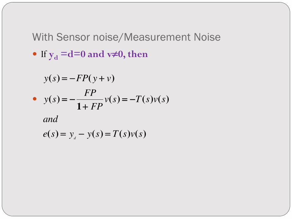
With Sensor noise/Measurement Noise

If yd =d=0 and v0, then

)()()()(

)()()(1

)(

)()(

svsTsyyse

and

svsTsvFP

FPsy

vyFPsy

d

Norms are Performance Measures

Signal forms and Signal Norms

Norm based approach for control design gives a sound platform for robust control designs

Different types of norms are used in control systems

Use would be depending on the mathematical approaches used to define the norm

Norms of signals and systems

Euclidean Norm or l2 norm for vector x is given as

For a vector signal x(t), l2 norm is

This norm is the square root of the energy in each component of the vector

If norm exists x(t) l2

212

1

1

2

2)( xxxx

Tn

ii

21

2)()(

dttxtxx

T

Norms of signals and systems

For power signals, we may use the root mean square value(rms) norm

21

)()(2

1lim)(

T

T

T

T

dttxtxT

xrms

Frobenius Norm For an mxr matrix A, the Frobenius norm is defines as

It can be shown that

21

1 1

2

,2

m

i

r

jji

aA

)()(2

2

TTAAtrAAtrA

System Norm LTI systems are generalization of matrices-

A matrix operates on a vector to produce another vector

An LTI system operates on a signal to produce another signal

So, analogous to Frobenius norm, we can define the system norm

L2 Norm for LTI systems Let G(s) be an mxr matrix transfer function Then the L2 norm for G(s) is defined as

||G||2 exists if an only if each element of G(s) is strictly proper. For SISO we have a scalar TF which need to be strictly proper. There should not any poles on the imaginary axis for either case.

Then we say G L2

2

1

2)()(

2

1

djGjGtrGT

G(s) plane in H2

When G L2 we can write the norm with respect to complex s plane as

dssGsGtrj

dssGsGtrj

G

T

T

))()((2

1

))()((2

12

2

Contour of integration for the last integral is along the entire imaginary axis and the infinite semicircle in the LHP or RHP

Since G(s) is strictly proper, it is easily shown that the integral vanishes over the semicircle

If G L2 and in addition, G is stable, then we say that G H2

H2 is the Hardy Space defined with the 2-norm

Exercise Calculate the L2 norm of G(s) given as:

)2(2

)2()3(

23

1)(

2

s

ss

sssG

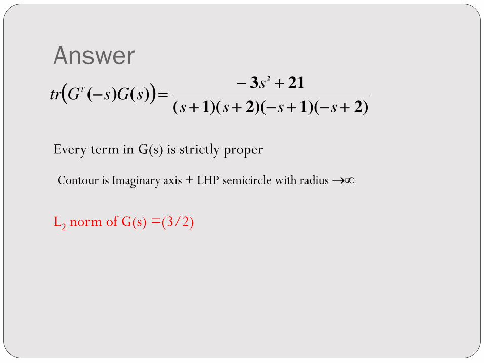
Answer

)2)(1)(2)(1(

213)()(

2

ssss

ssGsGtr

T

Every term in G(s) is strictly proper

Contour is Imaginary axis + LHP semicircle with radius

L2 norm of G(s) =(3/2)

Induced norm Induced norm is a different type of norm which applies to

operators and is essentially a type of “maximum gain” For a matrix, the induced Euclidean norm is

=sqrt(eigen(ATA))

)(

max212

2

A

AdAdi

)min(is and )max( the is

Induced norm for LTI system

To obtain induced norm for an LTI system, consider first a stable, strictly proper SISO system

Then, if the input u(.) l2 , then the output y(.) l2

By Parseval’s theorem

(A) )()(

2

1 222

2

djujGy

Clearly

Or

We argue that the RHS of the inequality in (B) can be reached arbitrarily closely for a fixed value of ||u||2 that is chosen to be 1 with no loss of generality

djujGy222

2)(

2

1)(sup

(B) )(sup2

2

22

2ujGy

Suppose |u(j)|2 approach an impulse of weight 2 in the frequency domain at = 0

Then the integral of Eq(A)

will approach

(A) )()(2

1 222

2

djujGy

2

0)( jG

If has a maximum at some finite value of , we may choose 0 to be that frequency

If not, then must approach a supremum as

.

We can make 0 as large as we like and will be as close to the supremum as we wish

The RHS of inequality in (B) can be reached arbitrarily closely and we get

)( jG

)( jG

)(0

jG

)(supsup2

12

jGyu

Hinfinity Norm

The norm calculated last is also the infinity norm given by

The infinity norm of G(s) exists if and only if G is proper with no poles on the j axis

In that case we write G L If in addition, G is stable, then we say G H

pp

pjGG

1

))((lim

H is the Hardy Space defined with the -norm

Norms for Multivariable systems

H norm for Multivariable systems

For multivariable systems, we have

This can be written as

djujGy2

2

2)()(

2

1

djujGy2

22

2)())](([

2

1

Further, we may write as

Or

djujGy2

2

22

2)(

2

1)((sup

2

2

22

2)]([sup ujGy

Contd… The factor ||u(j)||2 in the integrand refers to the 2-norm

of the vector u(j)

In SISO, the equivalent term refers to the 2-norm of a signal

We argue that the RHS of the last inequality

can be approached arbitrarily closely, by propoer choice of u(j)

2

2

22

2)]([sup ujGy

Essentially we pick u(j) to be the eigenvector of G*(j)G(j) corresponding to the largest eigenvalue, and we concentrate the spectrum of u(j) at the frequency where is the largest (or for some frequency that is arbitrarily large, if has no maximum, but a supremum. Therefore

)]([supsup2

12

jGyu

MIMO H norm As a continuation of the development, we define

)]([sup

jGG

Disturbance Rejection

Disturbance Rejection Disturbance rejection is a performance measure

Effect of disturbance is studied in two ways Input disturbance

Output disturbance

Rejection of Input disturbance

G yd

y u +

-

H

+

d

Analysis

GH1

G)s(T

and

GH1

G)s(T

d

yd

To suppress disturbance, we want |Td|<<1 For this we need |G|<<1 Keep |G(j)| small where d(t) contains stronger

components in the spectrum

Rejection of Output Disturbance

G yd

y u +

-

H

+

d

+

Analysis We have

To suppress disturbance, we want |Td|<<1

For this we need |G|>>1

Keep |G(j)| large where d(t) contains stronger components in the spectrum

GH1

1)s(T

and

GH1

G)s(T

d

yd

Contradiction The requirements to suppress disturbance at the input is

opposite to that needed for suppressing disturbance at the output

If the disturbance is present both at input and output we need to use some innovative ways to suppress both the disturbances

Noise Rejection

G yd

y u +

-

H +

n

+

Analysis

GH1

GH)s(T

and

GH1

G)s(T

n

yd

To suppress noise, we want |Tn|<<1 For this, we need |G|<<1for a given H Keep |G(j)| small where n(t) contains stronger

components in the spectrum

Exercise

G yd

y u +

-

H

K

Derive the Sensitivity and Complimentary Sensitivity Functions with respect to of the system given as G(s). G(s) is containing Uncertainty

Modeling the Uncertain Systems

Modeling the Uncertainties/perturbations

Uncertainties occur in control systems occur due to variety of reasons

Actually, the purpose of control system itself is to deal with uncertainties

Purpose of robust control is to render stability & acceptable performance if the uncertainties of certain class occur

Structured Uncertainty Interval Models

State Space model

Transfer function model

Unstructured Uncertainty Unstructured uncertainty is modeled, using the perturbation

approach, rather than representing the parameters using the intervals

There are different formulations that give the uncertain models, mostly use the norm bounds and the perturbations in the additive or multiplicative forms

General Basis Given a set of plants P with uncertainty in the parameters. A plant

transfer function P(,s)P is a transfer function admissible to represent the uncertain system being considered.

P0(0,s) P is one such plant with nominal values of the parameters, where 0 stands for the nominal value of the parameter set(vector)

0 could be the mean value of in the interval [min, max], which is intuitively appealing

Uncertainty could then be given as = 0[1+]

0 =(1/2)(min+max) & = (min -max)/ (min+max)

||1 is the perturbation

Unmodeled dynamics Uncertainty due to neglected and unmodeled dynamics is

more difficult to quantify

The frequency domain is well suited for representing this class of uncertainty through complex perturbations, which are normalized such that ||||1 where |||| is the

H norm of = )(sup

j

Classification of unstructured

uncertainty-SISO

Additive Uncertainty

Multiplicative Uncertainty

Inverse Multiplicative Uncertainty

Division Uncertainty

Use of the Uncertainty is depending on the problem being considered and the designer’s skill.

For MIMO systems, the constraints of pre and post multiplication gives rise to more classes of uncertainty

Additive Uncertainty Let us sue the property

P0(0,s) P is one such plant with nominal values of the parameters, where 0 stands for the nominal value of the parameter set(vector)

Let P(,s)= P0(0,s) +P(s)

P(s) is the complex perturbation applied to obtain the class of uncertain plants P(,s) and is stable

Then P(,s) is given in the Additive Uncertainty form

Usually, this is written as

P:Gp(s)=G(s)+wa(s) a(s) with ||||1

Example Consider the system

P: Gp(s)=AG (s). The uncertainty is in the Gain A and is given as A[Amin ,Amax]

Let A0 =(1/2)(Amin+Amax)

A= (Amin -Amax)/ (Amin+Amax)

A= A0[1+ A ]

Gp(s)= A0[1+ A ] G (s)=A0 G (s)+ A0 A G (s)

Multiplicative Uncertainty Let P(,s)= P0(0,s) + P0(0,s) P(s)

Or P(,s)= P0(0,s)(1+ P(s))

Or P(,s)= P0(0,s)[1+ wm(s) m(s)] ||||1

Example P: Gp(s)=AG (s). The uncertainty is in the Gain A and is given

as A[Amin ,Amax]

Let A0 =(1/2)(Amin+Amax)

A= (Amin -Amax)/ (Amin+Amax)

A= A0[1+ A ]

Gp(s)= A0 [1+ A ] G (s)=A0G (s) [1+ A ]

General method to find the Additive &

Multiplicative Uncertainty Model

Examples have shown the derivation of unstructured uncertainty from parametric uncertainty

This is simple for simple cases but

Tough for high order systems with uncertainty in many parameters, because Assumption about model and parameters may be inexact

The exact model structure is indispensable

Unmodeled dynamics cannot be then handled

Method

Given a model with uncertainties

Choose a nominal model(or lower order or delay free or a model of mean parameters or the central plant obtained from Nyquist plot corresponding to all plants in the given set)

For Additive uncertainty, find the smallest radius l a() which includes all possible plants such that

l a() =|Gp(j)-G (j)| Find a rational lower order transfer function wa(s) which is the

uncertainty weight such that |wa (j)| l a()

The uncertain additive plants Gp(s)=G(s)+wa (s) a(s)

Contd… In the case of multiplicative uncertainty, find the smallest

radius l a() such that for all possible plants

l a()=

For a chosen rational weight wm(s), there must be

)(

)()(max

jG

jGjGp

PGp

|wm (j)| l m()

Then Gp(s)=G(s)(1+wm(s) m(s))

Block diagram forms of uncertainty

Additive Uncertainty Model

G(s)

a (s) wa(s)

+

+

Multiplicative Uncertainty

G(s)

m (s) wm(s)

+

+

Inverse Multiplicative

G(s)

im (s) wim(s)

+ +

Division Uncertainty Consider the

It is easy to see that =0.6+0.3 with ||1

0.80.4 with 1

1)(

2

sssG

p

16.0

1)(

2

sssGp

2.0)( sswd

1

)]()(1)[()( 1

sGswsGsG dp

Robust Control

Robust Control Normally Robust control design considers two aspects

Robust Stability(RS)

Robust Performance(RP)

As a bottom line we need

Nominal stability(NS) and

Nominal performance(NP)

Robust Stability? How far the uncertainty can be, without violating the

stability, if the nominal system is stable?

(-1,j0)

Nyquist Plot Im

Re

G(j)

?

|1+G(j)|

Robust Stability with Multiplicative Uncertainty

m(s)

G(s) yd

y

u

+

-

Wm(s)

+ +

K(s)

Gp(s)

Analysis

We have

Assume that the nominal plant is stable

Using Nyquist stability condition, we need

Or

1 )()()(G(s)

))()(1)(()(

mmm

mmp

ssGsw

sswsGsG

)(1)()( sGsGswm

1)(1

)()(

sG

sGswm

We have

For robust stability, we want

Or and using H-inf we have

1)()(

)]()(1)[()()(

)]()(1[)(1

1

sTsS

sGsKsGsKsT

sGsKsS

1)()(1

)()()(

sGsK

sGsKswm

,1)()( sTswm

1)()(

sTswm

Robust Performance We find the bounds on the Sensitivity Function S and/or

Complimentary Sensitivity Function T for the given bounds on Disturbance or Measurement noise

Doyle’s Theorem A necessary and sufficient condition for robust performance

is to satisfy the condition

121

TWSW

Books Prabha Kundur “Power System Stability & Control” Tata McGrawHill,

1994|2012

Richard C Dorf & Robert H Bishop, “Modern Control Systems” Addison Wesley, 1999

Pierre R. Belanger, “Control Engineering: A Modern Approach” Saunders College Publishing, 1995

John Dorsey, “Continuous & Discrete Time Control Systems”, McGrawHill International, 2002

Vladimir Zakian, “Control Systems Design-A new Framework”, Springer 2005