introduction to robotics - universidad veracruzana · introduction to robotics ... • the value of...
TRANSCRIPT

12/03/18
1
Introduction to Robotics
Ph.D. Antonio Marin-Hernandez
Artificial Intelligence Department Universidad Veracruzana Sebastian Camacho # 5
Xalapa, Veracruz Robotics Action and Perception
LAAS-CNRS 7, av du colonel Roche
Toulouse, France
Topics
• Introduction: Types of robots • Locomotion • Kinematics of Mobile Robots • Perception • Navigation • Localization • Path Planning • Task Planning

12/03/18
2
Mobile Robots: Kinematics
• Kinematics is the basic study of a dynamic system behavior
• It is necessary to understand the mechanical behavior in order to: – Design tasks – Create control software
• The problems with kinematics of mobile robots are very similar to those on robotics manipulation:
• Workspace. It defines the range of possible solutions – Manipulators. All poses of end-effectors relative
to their fixture to the environment – Mobile Robots. All poses of the robot in
reference to their environment
Mobile Robots: Kinematics

12/03/18
3
Mobile Robots: Kinematics
• The main difference between mobile robots and manipulators is the way as position is estimated.
• Manipulators: – Arm’s pose is a simple matter of understanding
the kinematics and measuring the position for their joints.
– Those measures can be obtained directly from their sensors
Mobile Robots: Kinematics
• For a Mobile robot, there is not a direct way to compute their instantaneous position.
• It must be integrate by motion over time – Slippage problems
12/03/18
4
Mobile Robots: Kinematics
• To understand the whole motion it’s n e c e s s a r y t o u n d e r s t a n d t h e contribution of each wheel. – Each wheel has motion constrains. – All those constrains and the geometry of the
robot are combined to restrict the complete motion of the mobile robot
Mobile Robots: Kinematics
• Robot pose representation • Considerations
– A rigid body with wheels – Works on an horizontal plane
• Three dimensions (x, y, θ) • There are more degrees of freedom
– Wheel axes, turn axes (castor wheels), etc.

12/03/18
5
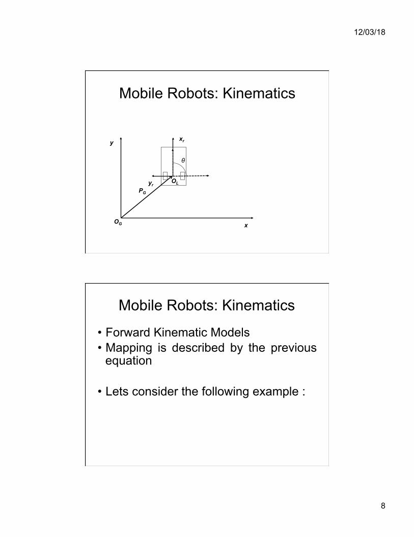
Mobile Robots: Kinematics
x
y
xr
y r
θ OL
PG
OG
OG= Global reference frame OL = Local reference frame PG = Position on OG
Mobile Robots: Kinematics • Axis x & y define the Global Reference
Frame OG • Axis xr & yr define the local reference frame
fixed to the robot • Pose of the robot in OG is given by :
– P = [ x y θ ]Τ

12/03/18
6
• To describe the motion in terms of their individual component it is necessary to map the motion in the local reference frame to the global reference frame.
• This mapping is a function of the current state of the robot.
• We must use the orthogonal rotation matrix
Mobile Robots: Kinematics
Mobile Robots: Kinematics
R(θ ) =cosθ sinθ 0−sinθ cosθ 00 0 1
"
#
$$$
%
&
'''
Orthogonal rotation Matrix
12/03/18
7
Mobile Robots: Kinematics
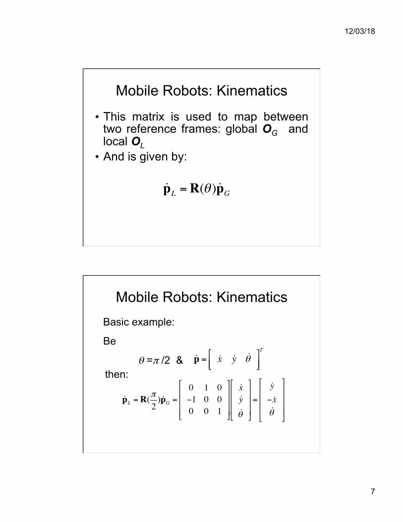
• This matrix is used to map between two reference frames: global OG and local OL • And is given by:
!pL =R(θ ) !pG
Mobile Robots: Kinematics
!pL =R(π2) !pG =
0 1 0−1 0 00 0 1
"
#
$$$
%
&
'''
!x!y!θ
"
#
$$$
%
&
'''=
!y− !x!θ
"
#
$$$
%
&
'''
Basic example:
Be
θ =π /2 & !p = !x !y !θ!"#
$%&
T
then:
12/03/18
8
Mobile Robots: Kinematics
x
y xr
yr
θ
OL
PG
OG
• Forward Kinematic Models • Mapping is described by the previous
equation • Lets consider the following example :
Mobile Robots: Kinematics

12/03/18
9
• A diferential model • Each wheel has a radio r and these are at
distance l • Given r, l, θ and the angular speeds of each
wheel, we have :
!p =!x!y!θ
!
"
###
$
%
&&&= f l, r,θ, !ϕ1, !ϕ2( )
Mobile Robots: Kinematics
• Then, its possible to compute the motion in the Global reference frame from local reference frame by :
!pG =R(θ )−1 !pL
Mobile Robots: Kinematics

12/03/18
10
Mobile Robots: Kinematics
x
y
xr
y r
θ OL
ω(t)
OG
v(t)
• Lets begin with some examples. • Suppose the local reference frame is
initially aligned with the global reference frame.
• Then, if only one wheel moves, the geometric center of the robot who is in the center of the axis between wheels, will move at half the speed of the moving wheel.
Mobile Robots: Kinematics

12/03/18
11
Mobile Robots: Kinematics
x
y
yr
OL
OG
V1
Vr
V2= 0
• For each wheel we have: & Then the tangential speed of the robot is
given by:
Mobile Robots: Kinematics
!xr1 =12r !ϕ1 !xr2 =
12r !ϕ2
!xr = !xr1 + !xr2
12/03/18
12
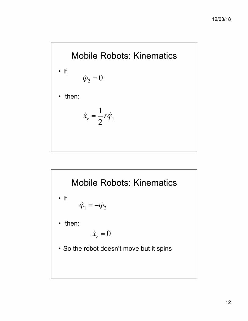
• If
• then:
Mobile Robots: Kinematics
!xr =12r !ϕ1
!ϕ2 = 0
• If
• then:
• So the robot doesn’t move but it spins
Mobile Robots: Kinematics
!xr = 0
!ϕ1 = − !ϕ2
12/03/18
13
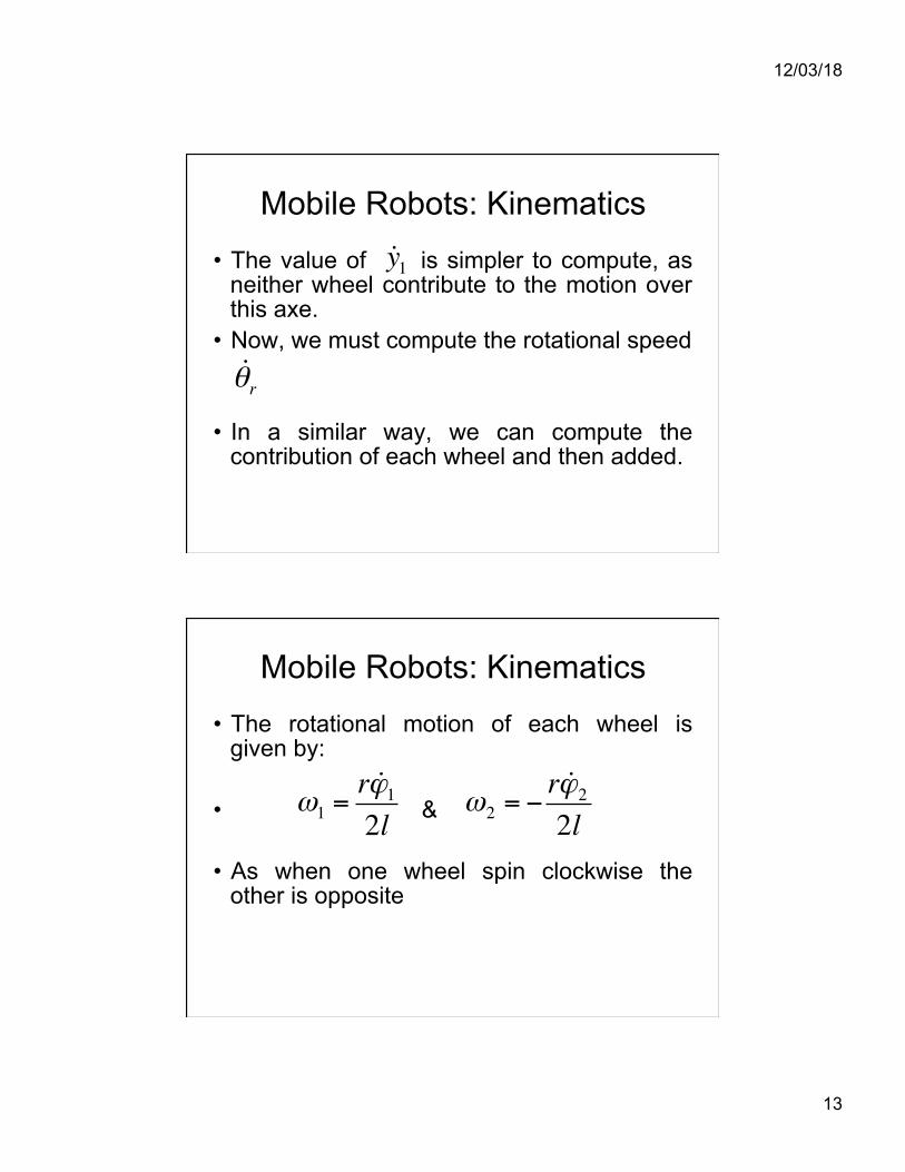
• The value of is simpler to compute, as neither wheel contribute to the motion over this axe.
• Now, we must compute the rotational speed
• In a similar way, we can compute the contribution of each wheel and then added.
Mobile Robots: Kinematics
!θr
!y1
• The rotational motion of each wheel is given by:
• &
• As when one wheel spin clockwise the other is opposite
Mobile Robots: Kinematics
ω1 =r !ϕ12l
ω2 = −r !ϕ22l

12/03/18
14
• In a similar way, we can compute the independent contribution of each wheel and then added.
Mobile Robots: Kinematics
!θ = r !ϕ12l
−r !ϕ22l
And then the complete motion will be given by:
Mobile Robots: Kinematics
!pG =R(θ )−1
r !ϕ12+r !ϕ22
0r !ϕ12l
−r !ϕ22l
⎡
⎣
⎢⎢⎢⎢⎢⎢
⎤
⎦
⎥⎥⎥⎥⎥⎥
12/03/18
15
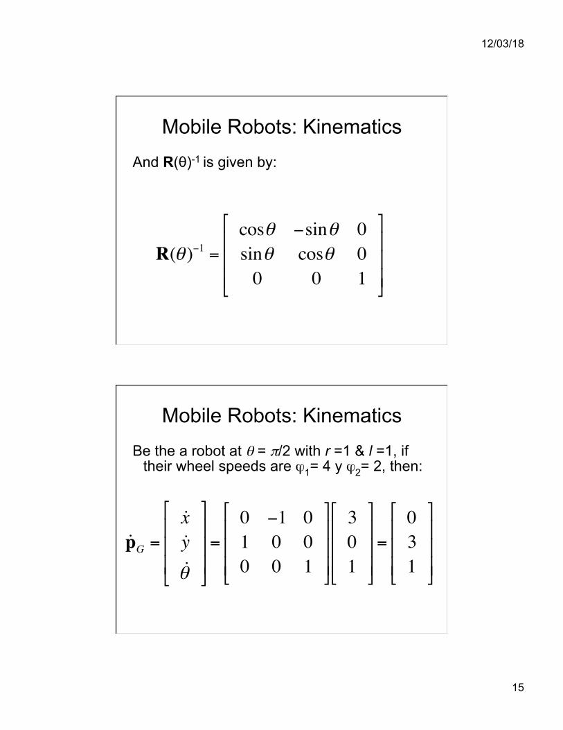
And R(θ)-1 is given by:
Mobile Robots: Kinematics
R(θ )−1 =cosθ −sinθ 0sinθ cosθ 00 0 1
⎡
⎣
⎢⎢⎢
⎤
⎦
⎥⎥⎥
Be the a robot at θ = π/2 with r =1 & l =1, if their wheel speeds are ϕ1= 4 y ϕ2= 2, then:
Mobile Robots: Kinematics
!pG =!x!y!θ
⎡
⎣
⎢⎢⎢
⎤
⎦
⎥⎥⎥=
0 −1 01 0 00 0 1
⎡
⎣
⎢⎢⎢
⎤
⎦
⎥⎥⎥
301
⎡
⎣
⎢⎢⎢
⎤
⎦
⎥⎥⎥=
031
⎡
⎣
⎢⎢⎢
⎤
⎦
⎥⎥⎥
12/03/18
16
• Wheels kinematic constraints • As we have seen, first of all the kinematic
constraints of each wheel are modeled and then is possible to combine them to get the kinematic model of the whole robot.
• Basically there are 4 types of wheels. • Then we are going to analyze their
constraints.
Mobile Robots: Kinematics
• Several simplifications will be taking into account – The plane of the wheel is always vertical – There is only one single contact point for
each wheel – There is no slippage at the contact point.
Mobile Robots: Kinematics

12/03/18
17
• Fixed standard wheel • This wheel has not vertical axis of rotation • It’s angle to the robot is fixed • Motion is then limited along the wheel plane
and rotation along it’s contact point
Mobile Robots: Kinematics
• Another approach for kinematics computation
• Consider a Differential Drive Robot – Independently of which wheel turns, the robot
rotates about a point that lies on the common axis between two wheels.
– Varying the relative speed of the two wheels, the rotation point will change.
Mobile Robots: Kinematics

12/03/18
18
– At each instant of time, the point at which the robot rotates must have the property that, left and right wheels follow a path that moves around the ICC at the same angular speed ω ant then:
– Where l is the de distance between the center of two wheels and R is the signed distance from the ICC to the midpoint between wheels
Mobile Robots: Kinematics
ω R+ l2
⎛
⎝⎜
⎞
⎠⎟= vr ω R− l
2⎛
⎝⎜
⎞
⎠⎟= vl
• Note that vr, vl, ω and R are functions of time.
• Solving for ω and R we get:
Mobile Robots: Kinematics
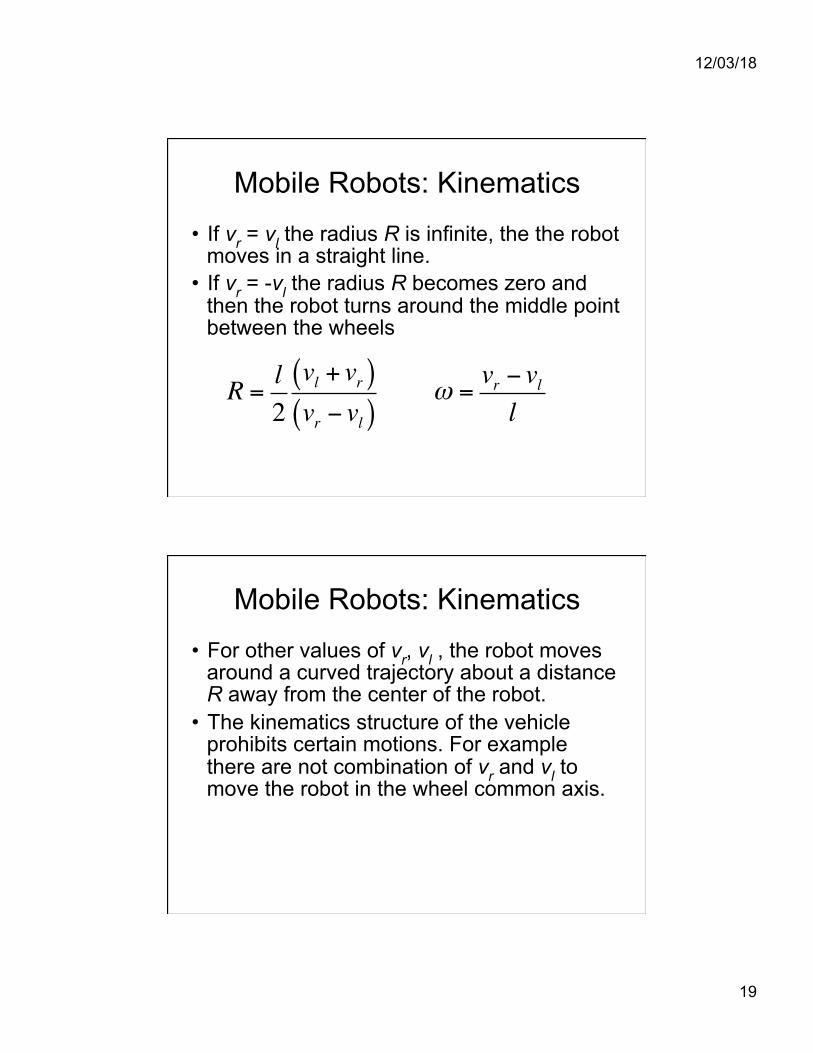
R = l2vl + vr( )vr − vl( )
ω =vr − vll
12/03/18
19
• If vr = vl the radius R is infinite, the the robot moves in a straight line.
• If vr = -vl the radius R becomes zero and then the robot turns around the middle point between the wheels
Mobile Robots: Kinematics
R = l2vl + vr( )vr − vl( )
ω =vr − vll
• For other values of vr, vl , the robot moves around a curved trajectory about a distance R away from the center of the robot.
• The kinematics structure of the vehicle prohibits certain motions. For example there are not combination of vr and vl to move the robot in the wheel common axis.
Mobile Robots: Kinematics

12/03/18
20
• A differential drive robot is very sensitive to the relative speeds of the wheels.
• Small errors in the velocity provided to each wheel result in different trajectories.
• Differential drive robots are sensitive to slight variations in the ground plane.
Mobile Robots: Kinematics
• Forward Kinematics • Suppose the robot at the given position
(x, y, θ) • Throughout manipulation of control
parameters vr and vl, the robot can be on different poses.
• Determining the pose that is reachable given the control parameters is known as the forward kinematics problem
Mobile Robots: Kinematics
12/03/18
21
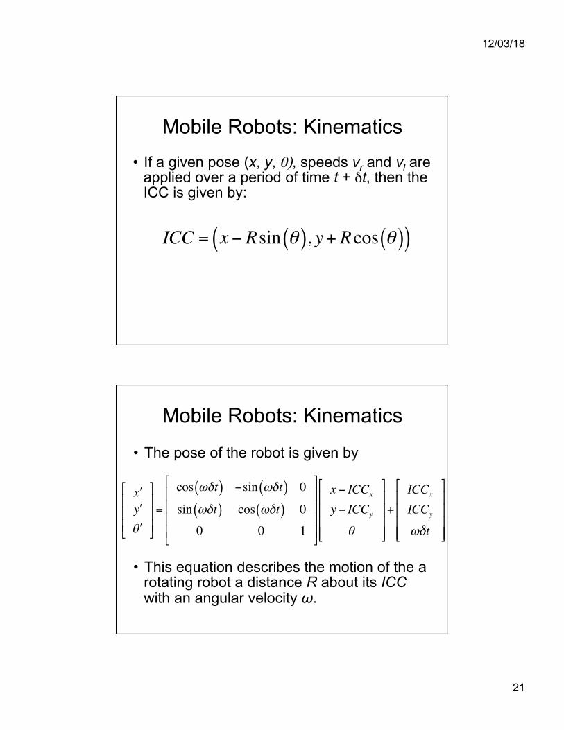
• If a given pose (x, y, θ), speeds vr and vl are applied over a period of time t + δt, then the ICC is given by:
Mobile Robots: Kinematics
ICC = x − Rsin θ( ), y+ Rcos θ( )( )
• The pose of the robot is given by
• This equation describes the motion of the a
rotating robot a distance R about its ICC with an angular velocity ω.
Mobile Robots: Kinematics
ʹxʹyʹθ
⎡
⎣
⎢⎢⎢
⎤
⎦
⎥⎥⎥=
cos ωδt( ) −sin ωδt( ) 0
sin ωδt( ) cos ωδt( ) 0
0 0 1
⎡
⎣
⎢⎢⎢⎢
⎤
⎦
⎥⎥⎥⎥
x − ICCx
y− ICCy
θ
⎡
⎣
⎢⎢⎢⎢
⎤
⎦
⎥⎥⎥⎥
+
ICCx
ICCy
ωδt
⎡
⎣
⎢⎢⎢⎢
⎤
⎦
⎥⎥⎥⎥
12/03/18
22
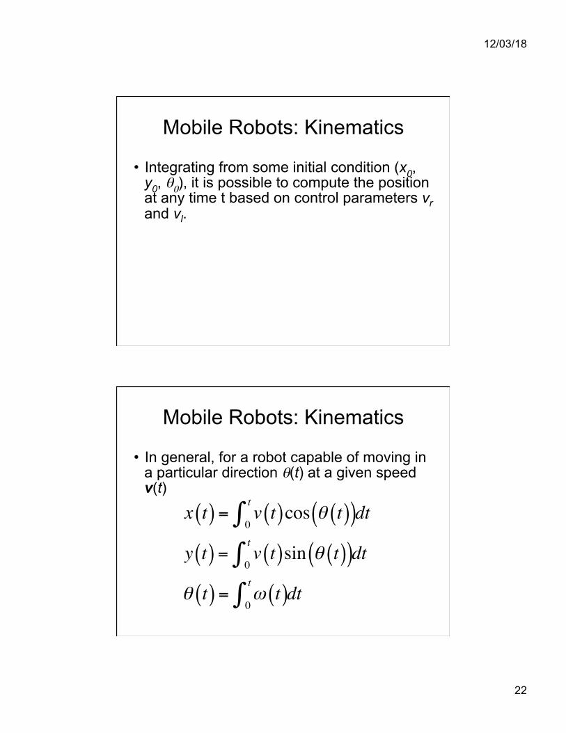
• Integrating from some initial condition (x0, y0, θ0), it is possible to compute the position at any time t based on control parameters vr and vl.
Mobile Robots: Kinematics
• In general, for a robot capable of moving in a particular direction θ(t) at a given speed v(t)
Mobile Robots: Kinematics
x t( ) = v t( )cos θ t( )( )0
t∫ dt
y t( ) = v t( )sin θ t( )( )0
t∫ dt
θ t( ) = ω t( )0
t∫ dt

12/03/18
23
• And for the special case of a differential robot we have:
Mobile Robots: Kinematics
x t( ) = 12
vr t( )+ vl t( )( )cos θ t( )( )0
t∫ dt
y t( ) = 12
vr t( )+ vl t( )( )sin θ t( )( )0
t∫ dt
θ t( ) = 1l
vr t( )− vl t( )( )0
t∫ dt
• However, what is more interesting is: • How to select the parameters to make the
robot to arrive at a desired position or to follow a given path.
• That is know as inverse kinematics • This is also related with path planning
Mobile Robots: Kinematics

12/03/18
24
• Inverse Kinematics • The previous equations describe the
constraints on the velocity of the robot that cannot be integrated into a position constraint
• This is know as non-holonomic constraint and is very difficult to solve.
• There are solutions for limited classes of the control functions.
Mobile Robots: Kinematics
• For example, if it is assumed vl(t) = vl, vr(t) =vr and vr≠ vl, we get:
where (x0, y0, θ0)= (0,0,0)
Mobile Robots: Kinematics
x t( ) = l2vr + vlvr − vl
sin tlvr − vl( )
⎛
⎝⎜
⎞
⎠⎟
y t( ) = − l2vr + vlvr − vl
cos tlvr − vl( )
⎛
⎝⎜
⎞
⎠⎟
θ t( ) = tlvr − vl( )

12/03/18
25
• Given a goal time t and a position (x, y), previous equations can be solved for vr and vl but does not provide for independent control of θ.
• Rather to invert previous equations to solve parameters that lead to a specific robot pose, it is possible to consider two special cases.
where (x0, y0, θ0)= (0,0,0)
Mobile Robots: Kinematics
• If vr = vl = v, then the robot’s motion simplifies to:
• The robot moves in a straight line
Mobile Robots: Kinematics
ʹxʹyʹθ
⎡
⎣
⎢⎢⎢
⎤
⎦
⎥⎥⎥=
x + vcos θ( )δty+ vsin θ( )δt
θ
⎡
⎣
⎢⎢⎢⎢
⎤
⎦
⎥⎥⎥⎥
12/03/18
26
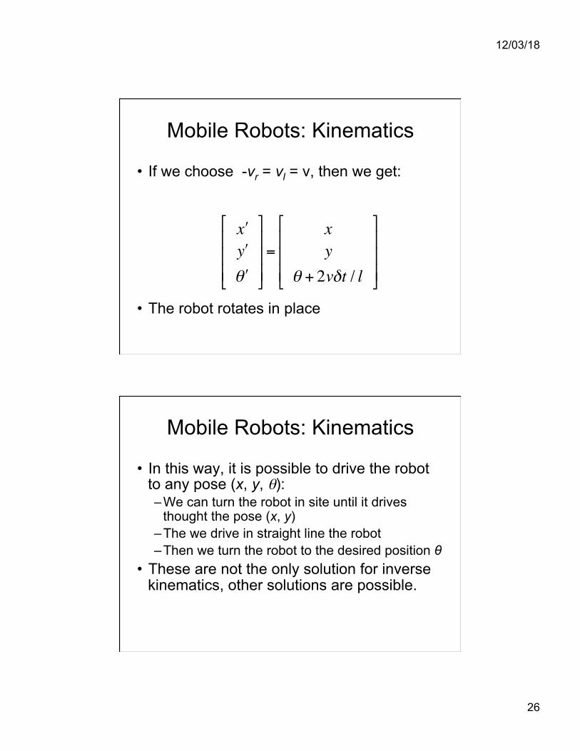
• If we choose -vr = vl = v, then we get:
• The robot rotates in place
Mobile Robots: Kinematics
ʹxʹyʹθ
⎡
⎣
⎢⎢⎢
⎤
⎦
⎥⎥⎥=
xy
θ + 2vδt / l
⎡
⎣
⎢⎢⎢
⎤
⎦
⎥⎥⎥
• In this way, it is possible to drive the robot to any pose (x, y, θ): – We can turn the robot in site until it drives
thought the pose (x, y) – The we drive in straight line the robot – Then we turn the robot to the desired position θ
• These are not the only solution for inverse kinematics, other solutions are possible.
• The robot rotates in place
Mobile Robots: Kinematics

12/03/18
27
Bibliography
• Siegwart R. and I. Nourbakhsh, “Introduction to Autonomous Mobile Robots”,MIT Press, 2004.
• Dudek G. and M. Jenkin, “Computational Principles of Mobile Robotics”, Cambridge University Press, 2000.
Bibliography • Ulrich Nehmzow, “Scientific Methods in Mobile
Robotics”, Springer, 2006. • Sebastian Thrun, Wolfram Burgard, and Dieter
Fox, “Probabilistic Robotics”, MIT Press, 2005. • Howie Choset, Kevin M. Lynch, Seth Hutchinson,
George Kantor, Wolfram Burgard, Lydia E. Kavraki, Sebastian Thrun,“Principles of Robot Motion: Theory, Algorithms, and Implementations”, MIT Press, 2005