introduction to robot sensors

7Introduction to Robot Sensors

The three main pillars of robotic autonomy can broadly be characterized asperception, planning, and control (i.e. the “see, think, act” cycle). Perceptioncategorizes those challenges associated with a robot sensing and understandingits environment, which are addressed by using various sensors and then extract-ing meaningful information from their measurements. The next few chapterswill focus on the perception/sensing problem in robotics, and in particular willintroduce common sensors utilized in robotics, their key performance charac-teristics, as well as strategies for extracting useful information from the sensoroutputs.

Introduction to Robot Sensors

Robots operate in diverse environments and often require diverse sets of sensorsto appropriately characterize them. For example, a self-driving car may utilizecameras, stereo cameras, lidar, and radar. Additionally, sensors are also requiredfor characterizing the physical state of the vehicle itself, for example wheelencoders, heading sensors, GNSS positioning sensors1, and more2. 1 Global Navigation Satellite System

2 R. Siegwart, I. R. Nourbakhsh, and D.Scaramuzza. Introduction to AutonomousMobile Robots. MIT Press, 2011

7.1 Sensor Classifications

To distinguish between sensors that measure the environment and sensors thatmeasure quantities related the robot itself, sensors are categorized as eitherproprioceptive or exteroceptive.

Definition 7.1.1 (Proprioceptive). Proprioceptive sensors measure values internalto the robot, for example motor speed, wheel load, robot arm joint angles, and batteryvoltage.

Definition 7.1.2 (Exteroceptive). Exteroceptive sensors acquire information from therobot’s environment, for example distance measurements, light intensity, and soundamplitude.

Generally speaking, exteroceptive sensor measurements are often more likelyto require interpretation by the robot in order to extract meaningful environ-

2 introduction to robot sensors

mental features. In addition to characterizing what the sensor measures, it isalso useful to characterize sensors based on how they operate. In particular it iscommon to characterize a sensor as either passive or active.

Definition 7.1.3 (Passive Sensor). Passive sensors measure ambient environmentalenergy entering the sensor, for example thermometers and cameras.

Definition 7.1.4 (Active Sensor). Active sensors emit energy into the environmentand measure the reaction, for example ultrasonic sensors and laser rangefinders.

Classifying a sensor as active or passive is important because this propertyintroduces unique challenges. For example the performance of passive sensorsdepend heavily on the environment, such as a camera being dependent on theambient lighting to get a good image.

7.2 Sensor Performance

Different types sensors also have different types of performance characteristics.Some sensors provide extreme accuracy in well-controlled laboratory settingsbut are overcome with error when subjected to real-world environmental vari-ations. Other sensors provide narrow, high-precision data in a wide variety ofsettings. In order to quantify and compare such performance characteristics it isnecessary to define relevant metrics. These metrics are generally either relatedto design specifications or in situ performance (i.e. how well a sensor performs inthe real environment).

7.2.1 Design Specification Metrics

A number of performance characteristics are specifically considered when de-signing the sensor, and are also used to quantify its overall nominal perfor-mance capabilities.

1. Dynamic range quantifies the ratio between the lower and upper limits of thesensor inputs under normal operation. This metric is usually expressed indecibels (dB), which is computed as

DR = 10 log10(r) [dB],

where r is the ratio between the upper and lower limits. In addition to dy-namic range (ratio), the actual range is also an important sensor metric. Forexample, an optical rangefinder will have a minimum operating range andcan thus provide spurious data when measurements are taken with the objectcloser than that minimum.

2. Resolution is the minimum difference between two values that can be de-tected by a sensor. Usually, the lower limit of the dynamic range of a sensoris equal to its resolution. However, this is not necessarily the case for digitalsensors.

principles of robot autonomy 3

3. Linearity characterizes whether or not the sensor’s output depends linearlyon the input.

4. Bandwidth or frequency is used to measure the speed with which a sensorcan provide a stream of readings. This metric is usually expressed in unitsof Hertz (Hz), which is measurements per second. High bandwidth sensorsare usually desired so that information can be updated at a higher rate. Forexample, mobile robots may have a limit on their maximum speed based onthe bandwidth of their obstacle detection sensors.

7.2.2 In Situ Performance Metrics

Metrics related to the design specifications can be reasonably quantified in alaboratory environment and then extrapolated to predict performance duringreal-world deployment. However, a number of important sensor metrics cannotbe adequately characterized in laboratories settings since they are influenced bycomplex interactions between the environment.

1. Sensitivity defines the ratio of change in the output from the sensor to achange in the input. High sensitivity is often undesirable because any noiseto the input can be amplified, but low sensitivity might degrade the ability toextract useful information from the sensor’s measurements. Cross-sensitivitydefines the sensitivity to environmental parameters that are unrelated to thesensor’s target quantity. For example, a flux-gate compass can demonstratehigh sensitivity to magnetic north and is therefore useful for mobile robotnavigation. However, the compass also has high sensitivity to ferrous build-ing materials, so much so that its cross-sensitivity often makes the sensoruseless in some indoor environments. High cross-sensitivity of a sensor isgenerally undesirable, especially when it cannot be modeled.

2. Error of a sensor is defined as the difference between the sensor’s outputmeasurements and the true values being measured, within some specificoperating context. Given a true value v and a measured value m, the error isdefined as e := m− v.

3. Accuracy is defined as the degree of conformity between the sensor’s mea-surement and the true value, and is often expressed as a proportion of thetrue value (e.g., 97.5% accuracy). Thus small error corresponds to high accu-racy and vice versa. For a measurement m and true value v, the accuracy isdefined as a := 1− |m− v|/v. Since obtaining the true value v can be difficultor impossible, characterizing sensor accuracy can be challenging.

4. Precision defines the reproducibility of the sensor results. For example, a sen-sor has high precision if multiple measurements of the same environmentalquantity are similar. It is important to note that precision is not the same asaccuracy, a highly precise sensor can still be highly inaccurate.


7.2.3 Sensor Errors

When discussing in situ performance metrics such as accuracy and precision, itis often important to also be able to reason about the sources of sensor errors.In particular it is important to distinguish between two main types of error,systematic errors and random errors.

1. Systematic errors are caused by factors or processes that can in theory be mod-eled (i.e. they are deterministic and therefore reproducible and predictable).Calibration error is a classic source of systematic error in sensors.

2. Random errors cannot be predicted using a sophisticated model (i.e. they arestochastic and unpredictable). Hue instability in a color camera, spuriousrangefinding errors, and black level noise in a camera are all examples ofrandom errors.

In order to reliably use a sensor in practice it is useful to have a characteri-zation of the systematic and random errors, which could allow for correctionsto make the sensor more accurate and provide information about its precision.Quantifying the sensor error and identifying sources of error is referred to aserror analysis. Error analysis for a typical sensor might involve identifying allof the sources of systematic errors, modeling random errors (e.g. by Gaussiandistributions), and then propagating the errors from each identified source todetermine the overall impact on the sensor output.

Unfortunately, it is typically challenging to perform a complete error analy-sis in practice for several reasons. One of the main reasons is due to a blurringbetween systematic and random errors that is the result of changes to the oper-ating environment. For example, exteroceptive sensors on a mobile robot willhave constantly changing measurement sources as the robot moves through theenvironment, and could even be influenced by the motion of the robot itself.Therefore, an exteroceptive sensor’s error profile may be heavily dependent onthe particular environment and even the particular state of the robot! As a moreconcrete example, active ranging sensors tend to have failure modes that aretriggered largely by specific relative positions of the sensor and environmenttargets. For example, when oriented at specific angles to a smooth sheetrockwall a sonar sensor will produce specular reflections that result in highly in-accurate range measurements. During the motion of a robot, these particularrelative angles would likely occur at stochastic intervals and therefore this errorsource might be considered random. Yet, if the robot were to stop at the specificangle for inducing specular reflections, the error would be persistent and couldbe modeled as a systematic error. In summary, while systematic and randomsensor errors might be well defined in controlled settings, in practical settingscharacterizing error becomes a lot more challenging due to the complexity andquantity of potential error sources.


7.2.4 Modeling Uncertainty

If all sensor measurement errors were systematic and could be modeled thentheoretically they could be corrected for. However in practice this is not the caseand therefore some alternative representation of the sensor error is needed. Inparticular, characterizing uncertainty due to random errors is typically accom-plished by using probability distributions.

Since it is effectively impossible to know all of the sources of random errorfor a sensor it is common to make assumptions about what the distributionof the sensor error looks like. For example, it is commonly assumed that ran-dom errors are zero-mean and symmetric, or to go slightly further that theyare Gaussian. More broadly, it is commonly assumed that the distribution isunimodal. These assumptions are usually made because they simplify the mathe-matical tools used for performing theoretical analyses.

However, it is also crucial to understand the limitations of these assumptions.In fact, in many cases even the most broad assumptions (e.g. that the distribu-tion is unimodal) can be quite wrong in practice. As an example consider thesonar sensor once again. When ranging an object that reflects the sound signalwell, the sonar will exhibit high accuracy and the random errors will generallybe based on noise (e.g. from the timing circuitry). In this operating instance itmight be a perfectly fine assumption that the noise distribution is unimodal andperhaps even Gaussian. However, if the sonar sensor is moving through an en-vironment and is faced with materials that cause coherent reflection (rather thandirectly returning the sound signal to the sonar sensor) then overestimates ofthe distance to the object are likely. In this case, the error will be biased towardpositive measurement error and will be far from the correct value. Thereforeit can be seen that modeling the sonar sensor uncertainty over all operatingregimes of the robot would at least require a bimodal distribution in this case.Additionally, since overestimation is more common than underestimation, thedistribution should also be asymmetric. As a second example, consider rangingvia stereo vision. Once again, at least two modes of operation can be identified.If the stereo vision system correctly correlates two images, then the resultingrandom error will be caused by camera noise and will limit the measurementaccuracy. But the stereo vision system can also correlate two images incorrectly.In such a case stereo vision will exhibit gross measurement error, and one caneasily imagine such behavior violating both the unimodal and the symmetricassumptions.

7.3 Common Sensors on Mobile Robots

7.3.1 Encoders

Encoders are electro-mechanical devices that convert motion into a sequenceof digital pulses, which can then be converted to relative or absolute positionmeasurements. These sensors are commonly used for wheel/motor sensing


to determine rotation angle and rotation rate. Since these sensors have vastapplications outside of mobile robotics there has been substantial developmentin low-cost encoders that offer excellent resolution. In mobile robotics, encodersare one of the most popular means to control the position or speed of wheelsand other motor-driven joints. These sensors are proprioceptive and thereforetheir estimates are expressed in the reference frame of the robot.

Figure 7.1: Quadrature opticalwheel encoder. (Figure fromSiegwart et al.)

Optical encoders shine light onto a photodiode through slits in a metal orglass disc, and measure the sine or square wave pulses that result from diskrotation (see Figure 7.1). After some signal processing it is possible to integratethe number of wave peaks to determine how much the disk has rotated. En-coder resolution is measured in cycles per revolution (CPR) and the minimumangular resolution can be readily computed from an encoder’s CPR rating. Atypical encoder in mobile robotics may have 2000 CPR, while the optical en-coder industry can readily manufacture encoders with 10,000 CPR. In terms ofbandwidth, it is of course critical that the encoder is sufficiently fast to handlethe expected shaft rotation rates. Luckily, industrial optical encoders present nobandwidth limitation to mobile robot applications. Usually in mobile roboticsthe quadrature encoder is used. In this case, a second illumination and detec-tor pair is placed 90 degrees shifted with respect to the original in terms of therotor disc. The resulting twin square waves, shown in Figure 7.1, provide signif-icantly more information. The ordering of which square wave produces a risingedge first identifies the direction of rotation. Furthermore, the resolution is im-proved by a factor of four with no change to the rotor disc. Thus, a 2000 CPRencoder in quadrature yields 8000 counts.

As with most proprioceptive sensors, encoders typically operate in a verypredictable and controlled environment. Therefore systematic errors and cross-sensitivities can be accounted for. In practice, the accuracy of optical encodersis often assumed to be 100% since any encoder errors are dwarfed by errors indownstream components.

7.3.2 Heading Sensors

Heading sensors can be proprioceptive (e.g. gyroscopes, inclinometers) or exte-roceptive (e.g. compasses). They are used to determine the robot’s orientation inspace. Additionally, they can also be used to obtain position estimates by fusing


the orientation and velocity information and integrating, a process known asdead reckoning.

Compasses: Compasses are exteroceptive sensors that measure the earth’s mag-netic field to provide a rough estimate of direction. In mobile robotics, digitalcompasses using the Hall effect are popular and they are inexpensive but oftensuffer from poor resolution and accuracy. Flux gate compasses have improvedresolution and accuracy, but are more expensive and physically larger. Bothcompass types are vulnerable to vibrations and disturbances in the magneticfield, and are therefore less well suited for indoor applications.

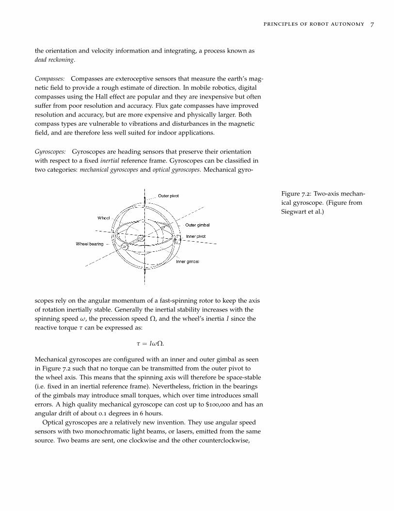
Gyroscopes: Gyroscopes are heading sensors that preserve their orientationwith respect to a fixed inertial reference frame. Gyroscopes can be classified intwo categories: mechanical gyroscopes and optical gyroscopes. Mechanical gyro-

Figure 7.2: Two-axis mechan-ical gyroscope. (Figure fromSiegwart et al.)

scopes rely on the angular momentum of a fast-spinning rotor to keep the axisof rotation inertially stable. Generally the inertial stability increases with thespinning speed ω, the precession speed Ω, and the wheel’s inertia I since thereactive torque τ can be expressed as:

τ = IωΩ.

Mechanical gyroscopes are configured with an inner and outer gimbal as seenin Figure 7.2 such that no torque can be transmitted from the outer pivot tothe wheel axis. This means that the spinning axis will therefore be space-stable(i.e. fixed in an inertial reference frame). Nevertheless, friction in the bearingsof the gimbals may introduce small torques, which over time introduces smallerrors. A high quality mechanical gyroscope can cost up to $100,000 and has anangular drift of about 0.1 degrees in 6 hours.

Optical gyroscopes are a relatively new invention. They use angular speedsensors with two monochromatic light beams, or lasers, emitted from the samesource. Two beams are sent, one clockwise and the other counterclockwise,


through an optical fiber. Since the laser traveling in the direction of rotation hasa slightly shorter path, it will have a higher frequency. This frequency differenceδ f is proportional to the angular velocity, which can therefore be estimated.In modern optical gyroscopes, bandwidth can easily exceed 100 kHz, whileresolution can be smaller than 0.0001 degrees/hr.

7.3.3 Accelerometer

An accelerometer is a device used to measure net accelerations (i.e. the net ex-ternal forces acting on the sensor, including gravity). Mechanical accelerometersare essentially spring-mass-damper systems that can be represented by the sec-ond order differential equation3: 3 G. Dudek and M. Jenkin. “Inertial

Sensors, GPS, and Odometry”. In:Springer Handbook of Robotics. Springer,2008, pp. 477–490

Fapplied = mx + cx + kx

where m is the proof mass, c is the damping coefficient, k is the spring constant,and x is the relative position to a reference equilibrium. When a static force isapplied, the system will oscillate until it reaches a steady state where the steadystate acceleration would be given as:

aapplied =kxm

.

The design of the sensor chooses m, c, and k such that system can stabilizequickly and then the applied acceleration can be calculated from steady state.Modern accelerometers, such as the ones in mobile phones, are usually verysmall and use Micro Electro-Mechanical Systems (MEMS), which consist of acantilevered beam and a proof mass. The deflection of the proof mass from itsneutral position is measured using capacitive or piezoelectric effects.

7.3.4 Inertial Measurement Unit (IMU)

Inertial measurement units (IMU) are devices that use gyroscopes and ac-celerometers to estimate their relative position, orientation, velocity, and ac-celeration with respect to an inertial reference frame. Their general workingprinciple is shown in Figure 7.3.

The gyroscope data is integrated to estimate the vehicle orientation while thethree accelerometers are used to estimate the instantaneous acceleration of thevehicle. The acceleration is then transformed to the local navigation frame bymeans of the current estimate of the vehicle orientation relative to gravity. Atthis point the gravity vector can be subtracted from the measurement. The re-sulting acceleration is then integrated to obtain the velocity and then integratedagain to obtain the position, provided that both the initial velocity and positionare a priori known. To overcome the need of knowing of the initial velocity, theintegration is typically started at rest when the velocity is zero.

One of the fundamental issues with IMUs is the phenomenon called drift,which describes the slow accumulation of errors over time. Drift in any one


component will also effect the downstream components as well. For example,drift in the gyroscope unavoidably undermines the estimation of the vehicle ori-entation relative to gravity, which results in incorrect cancellation of the gravityvector. Additionally, errors in acceleration measurements will cause the inte-grated velocity to drift in time (which will in turn also cause position estimatedrift). To account for drift periodic references to some external measurement isrequired. In many robot applications, such an external reference may come fromGNSS position measurements, cameras, or other sensors.

Figure 7.3: Inertial measure-ment unit (IMU) block diagram.

7.3.5 Beacons

Beacons are signaling devices with precisely known positions (e.g. stars andlighthouses are classic examples). Position of a mobile robot can be determinedby knowing the position of the beacon and by having access to relative positionmeasurements. The GNSS positioning system and camera-based motion capturesystem for indoor use are more advanced examples. GNSS based positioning isextremely popular in robotics, and works by processing synchronized signalsfrom at least four satellites. Signals from four satellites are needed (at a mini-mum) to enable the estimation of four unknown quantities (the three positioncoordinates plus a clock correction). Modified GNSS-based methods, such asdifferential GPS, can be used to increase positioning accuracy.

7.3.6 Active Ranging

Active ranging sensors provide direct measurements of distance to objects inthe vicinity of the sensor. These sensors are important in robotics for both lo-calization and environment reconstruction. There are two main types of activeranging sensors: time-of-flight active ranging sensors (e.g. ultrasonic, laserrangefinder, and time-of-flight cameras) and geometric active ranging sensors(e.g. based on optical triangulation and structured light).

Figure 7.4: The Velodyne HDL-64E High Definition Real-Time3D Lidar sensor, a time-of-flightactive ranging sensor. (Imageretrieved from velodyneli-dar.com)

Time-of-flight Active Ranging: Time-of-flight active ranging sensors make useof the propagation speed of sounds or electromagnetic waves. In particular, thetravel distance is given by

d = ct,


where d is the distance traveled, c is the speed of wave propagation, and t isthe time of flight. The propagation speed c of sound is approximately 0.3m/mswhereas the speed of electromagnetic signals is 0.3m/ns, which is 1 milliontimes faster! The time of flight for a distance of 3 meters is 10 milliseconds foran ultrasonic system, but only 10 nanoseconds for a laser rangefinder, whichmakes measuring the time of flight t for electromagnetic signals more techno-logically challenging. This explains why laser range sensors have only recentlybecome affordable and robust for use on mobile robots. The quality of differenttime-of-flight range sensors may depend on:

1. uncertainties in determining the exact time of arrival of the reflected signal,

2. inaccuracies in the time-of-flight measurement (particularly with laser rangesensors),

3. the dispersal cone of the transmitted beam (mainly with ultrasonic rangesensors),

4. interaction with the target (e.g. surface absorption, specular reflections),

5. variation of propagation speed,

6. the speed of the mobile robot and target (in the case of a dynamic target).

Geometric Active Ranging: Geometric active ranging sensors use geometricproperties in the measurements to establish distance readings. Generally, thesesensors project a known pattern of light and then geometric properties can beused to analyze the reflection and estimate range via triangulation. Opticaltriangulation sensors (1D) transmit a collimated (parallel rays of light) beamtoward the target and use a lens to collect reflected light and project it onto aposition-sensitive device or linear camera. Structured light sensors (2D or 3D)project a known light pattern (e.g. point, line, or texture) onto the environment.The reflection is captured by a receiver and then, together with known geomet-ric values, range is estimated via triangulation.

7.3.7 Other Sensors

Some classical examples of other sensors include radar, tactile sensors, andvision based sensors (e.g. cameras). Radar sensors leverage the Doppler effect toproduce velocity relative velocity measurements. Tactile sensors are particularlyuseful for robots that interact physically with their environment.

7.4 Computer Vision

Vision sensors have become crucial sensors for perception in the context ofrobotics. This is generally due to the fact that vision provides an enormous


amount of information about the environment and enables rich, intelligent inter-action in dynamic environments4. The main challenges associated with vision- 4 In fact, the human eye provides

millions of bits of information persecond.

based sensing are related to processing digital images to extract salient infor-mation like object depth, motion and object detection, color tracking, featuredetection, scene recognition, and more. The analysis and processing of imagesare generally referred to as computer vision and image processing. Tremendous ad-vances and new theoretical findings in these fields over the last several decadeshave led to sophisticated computer vision and image processing techniques tobe utilized in industrial and consumer applications such as photography, defectinspection, monitoring and surveillance, video games, movies, and more. Thissection introduces some fundamental concepts related to these fields, and inparticular will focus on cameras and camera models.

7.4.1 Digital Cameras

While the basic idea of a camera has existed for thousands of years, the firstclear description of one was given by Leonardo Da Vinci in 1502 and the oldestknown published drawing of a camera obscura (a dark room with a pinhole toimage a scene) was shown by Gemma Frisius in 1544. By 1685, Johann Zahnhad designed the first portable camera, and in 1822 Joseph Nicephore Niepcetook the first physical photograph.

Modern cameras consist of a sensor that captures light and converts the re-sulting signal into a digital image. Light falling on an imaging sensor is usuallypicked up by an active sensing area, integrated for the duration of the exposure(usually expressed as the shutter speed, e.g. 1/125, 1/60, 1/30 of a second), andthen passed to a set of sense amplifiers. The two main kinds of sensors used indigital cameras today are charge coupled devices (CCD) and complementarymetal oxide on silicon (CMOS) sensors. A CCD chip is an array of light-sensitivepicture elements (pixels), and can contain between 20,000 and several millionpixels total. Each pixel can be thought of as a light-sensitive discharging capac-itor that is 5 to 25µm in size. While complementary metal oxide semiconductor(CMOS) chips also consist of an array of pixels, they are quite different fromCCD chips. In particular, along the side of each pixel are several transistors spe-cific to that pixel. CCD sensors have typically outperformed CMOS for qualitysensitive applications such as digital single-lens-reflex cameras, while CMOSsensors are better for low-power applications. However, today CMOS sensorsare standard in most digital cameras.

7.4.2 Image Formation

Before reaching the camera’s sensor, light rays first originate from a light source.In general the rays of light reflected by an object tend to be scattered in manydirections and may consist of different wavelengths. Averaged over time, theemitted wavelengths and directions for a specific object can be precisely de-scribed using object-specific probability distribution functions. In particular,


the light reflection properties of a given object are the result of how light is re-flected, scattered, or absorbed based on the object’s surface properties and thewavelength of the light. For example, an object might look blue because bluewavelengths of light are primarily scattered off the surface while other wave-lengths are absorbed. Similarly, a black object looks black because it absorbsmost wavelengths of light, and a perfect mirror reflects all visible wavelengths.

Cameras capture images by sensing these light rays on a photoreceptive sur-face (e.g. a CCD or a CMOS sensor). However, since light reflecting off an objectis generally scattered in many directions, simply exposing a planar photorecep-tive surface to these reflected rays would result in many rays being capturedat each pixel. This would lead to blurry images! A solution to this issue is toadd a barrier in front of the photoreceptive surface that blocks most of theserays, and only lets some of them pass through an aperture (see Figure 7.5). Theearliest approach to filtering light rays in this way was to have a small hole inthe barrier surface. Cameras with this type of filter were referred to as pinholecameras.

Figure 7.5: Light rays on a pho-toreceptive surface referredto as the image plane. On theleft, numerous rays being re-flected and scattered by theobject leads to blurry imageswhereas (on the right), a bar-rier has been added so thatthe scattered light rays can bedistinguished.

7.4.3 Pinhole Camera Model

A pinhole camera has no lens but rather a single very small aperture. Lightfrom the scene passes through this pinhole aperture and projects an invertedimage onto the image plane (see Figure 7.6). While modern cameras do notoperate in this way, the principles of the pinhole camera can be used to deriveuseful mathematical models.

To develop the mathematical pinhole camera model, several useful referenceframes are defined. First, the camera reference frame is centered at a point O (seeFigure 7.6) that is at a focal length f in front of the image plane. This referenceframe with directions (i, j, k) is defined with the k axis coincident with the op-tical axis that points toward the image plane. The coordinates of a point in thecamera frame are denoted by uppercase P = (X, Y, Z). When a ray of lightis emitted from a point P and passes through the pinhole at point O, it getscaptured on the image plane at a point p. Since these points are all collinearit is possible to deduce the following relationships between the coordinatesP = (X, Y, Z) and p = (x, y, z):

x = λX, y = λY, z = λZ,


Figure 7.6: Pinhole cameramodel. Due to the geometry ofthe pinhole camera system, theobject’s image is inverted on theimage plane. In this figure, O isthe camera center, c is the im-age center, and p the principalpoint.

for some λ ∈ R. This leads to the relationship:

λ =xX

=yY

=zZ

.

Further, from the geometry of the camera it can be seen that z = f where f isthe focal length, such that these expressions can be rewritten as:

x = fXZ

, y = fYZ

. (7.1)

Therefore the position of the pixel on the image plane that captures a ray oflight from the point P can be computed.

7.4.4 Thin Lens Model

One of the main issues with having a fixed pinhole aperture is that there is atrade-off associated with the aperture’s size. A large aperture allows a greaternumber of light rays to pass through, which leads to blurring of the image.However, a small aperture lets through fewer light rays and the resulting imageis darker. As a solution, lenses can focus light via refraction and can be used toreplace the aperture, therefore avoiding the need for these trade-offs.

A similar mathematical model to the pinhole model can be introduced forlenses by using properties from Snell’s law. Figure 7.7 shows a diagram of themost basic lens model, which is the thin lens model (which assumes no opticaldistortion due to the curvature of the lens). Snell’s law states that rays passingthrough the center of the lens are not refracted, and those that are parallel to theoptical axis are focused on the focal point labeled F′. In addition, all rays pass-ing through P are focused by the thin lens on the point p. From the geometry ofsimilar triangles, a mathematical model similar to (7.1) is developed:

yY

=zZ

,yY

=z− f

f=

zf− 1, (7.2)

where again the point P has coordinates (X, Y, Z), its corresponding point p onthe image plane has coordinates (x, y, z), and f is the focal length. Combining


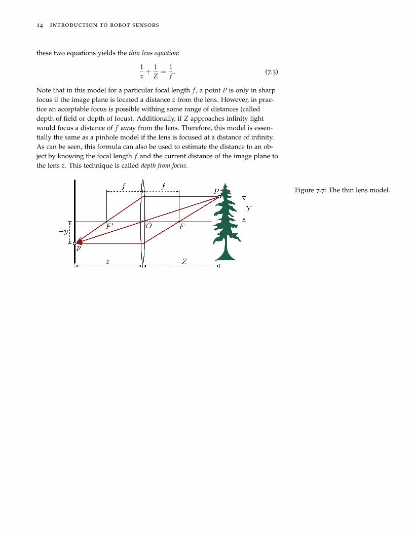
these two equations yields the thin lens equation:

1z+

1Z

=1f

. (7.3)

Note that in this model for a particular focal length f , a point P is only in sharpfocus if the image plane is located a distance z from the lens. However, in prac-tice an acceptable focus is possible withing some range of distances (calleddepth of field or depth of focus). Additionally, if Z approaches infinity lightwould focus a distance of f away from the lens. Therefore, this model is essen-tially the same as a pinhole model if the lens is focused at a distance of infinity.As can be seen, this formula can also be used to estimate the distance to an ob-ject by knowing the focal length f and the current distance of the image plane tothe lens z. This technique is called depth from focus.

Figure 7.7: The thin lens model.

Bibliography

[1] G. Dudek and M. Jenkin. “Inertial Sensors, GPS, and Odometry”. In:Springer Handbook of Robotics. Springer, 2008, pp. 477–490.

[2] R. Siegwart, I. R. Nourbakhsh, and D. Scaramuzza. Introduction to Au-tonomous Mobile Robots. MIT Press, 2011.

introduction to robot sensors

Documents