introduction to propensity score matching: a review and...
TRANSCRIPT
Introduction to Propensity ScoreMatching: A Review and Illustration
Shenyang Guo, Ph.D.School of Social Work
University of North Carolina at Chapel HillJanuary 28, 2005
For Workshop Conducted at the School of Social Work,University of Illinois – Urbana-Champaign
NSCAW data used to illustrate PSM were collected under funding by the Administration on Children, Youth, andFamilies of the U.S. Department of Health and Human Services. Findings do not represent the official position orpolicies of the U.S. DHHS. PSM analyses were funded by the Robert Wood Johnson Foundation Substance AbusePolicy Research Program, and by the Children’s Bureau’s research grant. Results are preliminary and notquotable. Contact information: [email protected]

OutlineDay 1• Overview:
• Why PSM?• History and development of PSM• Counterfactual framework• The fundamental assumption
• General procedure• Software packages• Review & illustration of the basic methods
developed by Rosenbaum and Rubin

Outline (continued)• Review and illustration of Heckman’s
difference-in-differences method• Problems with the Rosenbaum & Rubin’s method• Difference-in-differences method• Nonparametric regression• Bootstrapping
Day 2• Practical issues, concerns, and strategies• Questions and discussions

PSM References
Check website:
http://sswnt5.sowo.unc.edu/VRC/Lectures/index.htm
(Link to file “Day1b.doc”)

Why PSM? (1)Need 1: Analyze causal effects of
treatment from observational data• Observational data - those that are not generated
by mechanisms of randomized experiments, suchas surveys, administrative records, and census data.
• To analyze such data, an ordinary least square(OLS) regression model using a dichotomousindicator of treatment does not work, because insuch model the error term is correlated withexplanatory variable.

Why PSM? (2)
The independent variable w is usuallycorrelated with the error term ε. Theconsequence is inconsistent and biasedestimate about the treatment effect τ.
iiiiXWY !"#$ +++='

Why PSM? (3)Need 2: Removing Selection Bias in Program Evaluation• Fisher’s randomization idea.• Whether social behavioral research can really
accomplish randomized assignment of treatment?• Consider E(Y1|W=1) – E(Y0|W=0) . Add and subtract
E(Y0|W=1), we have {E(Y1|W=1) – E(Y0|W=1)} + {E(Y0|W=1) -
E(Y0|W=0)} Crucial: E(Y0|W=1) ≠ E(Y0|W=0)• The debate among education researchers: the impact
of Catholic schools vis-à-vis public schools onlearning. The Catholic school effect is the strongestamong those Catholic students who are less likely toattend Catholic schools (Morgan, 2001).

Why PSM? (4)Heckman & Smith (1995) Four Important Questions:• What are the effects of factors such as subsidies,
advertising, local labor markets, family income, race, andsex on program application decision?
• What are the effects of bureaucratic performancestandards, local labor markets and individualcharacteristics on administrative decisions to acceptapplicants and place them in specific programs?
• What are the effects of family background, subsidies andlocal market conditions on decisions to drop out from aprogram and on the length of time taken to complete aprogram?
• What are the costs of various alternative treatments?

History and Development of PSM• The landmark paper: Rosenbaum & Rubin (1983).• Heckman’s early work in the late 1970s on selection bias
and his closely related work on dummy endogenousvariables (Heckman, 1978) address the same issue ofestimating treatment effects when assignment isnonrandom.
• Heckman’s work on the dummy endogenous variableproblem and the selection model can be understood as ageneralization of the propensity-score approach (Winship& Morgan, 1999).
• In the 1990s, Heckman and his colleagues developeddifference-in-differences approach, which is a significantcontribution to PSM. In economics, the DID approach andits related techniques are more generally callednonexperimental evaluation, or econometrics of matching.

The Counterfactual Framework• Counterfactual: what would have happened to the treated
subjects, had they not received treatment?• The key assumption of the counterfactual framework is
that individuals selected into treatment and nontreatmentgroups have potential outcomes in both states: the one inwhich they are observed and the one in which they are notobserved (Winship & Morgan, 1999).
• For the treated group, we have observed mean outcomeunder the condition of treatment E(Y1|W=1) andunobserved mean outcome under the condition ofnontreatment E(Y0|W=1). Similarly, for the nontreatedgroup we have both observed mean E(Y0|W=0) andunobserved mean E(Y1|W=0) .

The Counterfactual Framework(Continued)
• Under this framework, an evaluation of E(Y1|W=1) - E(Y0|W=0) can be thought as an effort that uses E(Y0|W=0) to
estimate the counterfactual E(Y0|W=1). The centralinterest of the evaluation is not in E(Y0|W=0), but inE(Y0|W=1).
• The real debate about the classical experimentalapproach centers on the question: whether E(Y0|W=0)really represents E(Y0|W=1)?

Fundamental Assumption• Rosenbaum & Rubin (1983)
• Different versions: “unconfoundedness” &“ignorable treatment assignment” (Rosenbaum &Robin, 1983), “selection on observables” (Barnow,Cain, & Goldberger, 1980), “conditionalindependence” (Lechner 1999, 2002), and“exogeneity” (Imbens, 2004)
.|),( 10 XWYY !

1-to-1 or 1-to-n Match
Nearest neighbor matching
Caliper matching
Mahalanobis
Mahalanobis withpropensity score added
Run Logistic Regression:
• Dependent variable: Y=1, ifparticipate; Y = 0, otherwise.
•Choose appropriateconditioning (instrumental)variables.
• Obtain propensity score:predicted probability (p) orlog[(1-p)/p].
General Procedure
Multivariate analysis based on new sample
1-to-1 or 1-to-n matchand then stratification(subclassification)
Kernel or local linearweight match and thenestimate Difference-in-differences (Heckman)
Either
Or

Nearest Neighbor and CaliperMatching
• Nearest neighbor: The nonparticipant with the value of Pj that is
closest to Pi is selected as the match.• Caliper: A variation of nearest neighbor: A match
for person i is selected only if where ε is a pre-specified tolerance.
Recommended caliper size: .25σp• 1-to-1 Nearest neighbor within caliper (The is a
common practice)• 1-to-n Nearest neighbor within caliper
0|,|min)( IjPPPC jij
i !"=
0,|| IjPP ji !<" #
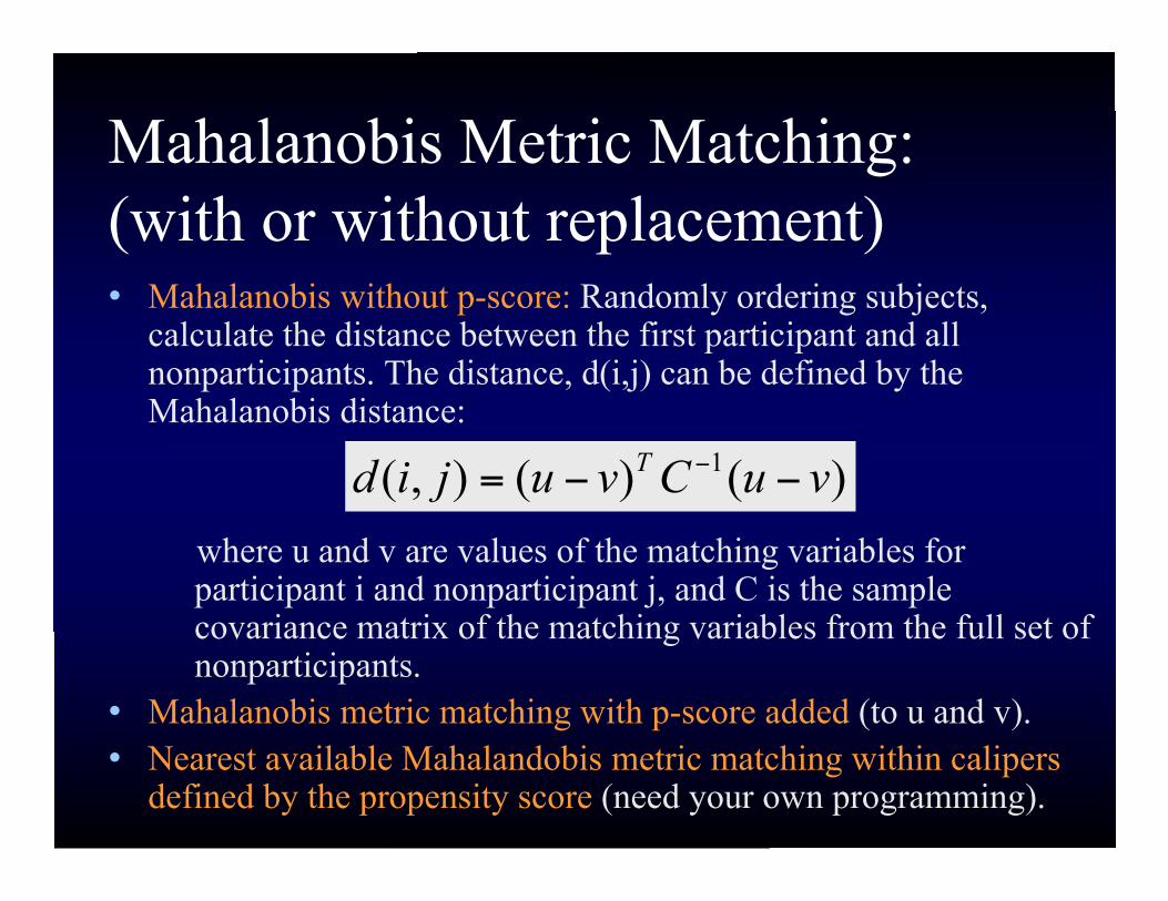
Mahalanobis Metric Matching:(with or without replacement)• Mahalanobis without p-score: Randomly ordering subjects,
calculate the distance between the first participant and allnonparticipants. The distance, d(i,j) can be defined by theMahalanobis distance:
where u and v are values of the matching variables forparticipant i and nonparticipant j, and C is the samplecovariance matrix of the matching variables from the full set ofnonparticipants.
• Mahalanobis metric matching with p-score added (to u and v).• Nearest available Mahalandobis metric matching within calipers
defined by the propensity score (need your own programming).
)()(),( 1 vuCvujid T!!=
!

Stratification (Subclassification)Matching and bivariate analysis are combined into one
procedure (no step-3 multivariate analysis):• Group sample into five categories based on
propensity score (quintiles).• Within each quintile, calculate mean outcome for
treated and nontreated groups.• Estimate the mean difference (average treatment
effects) for the whole sample (i.e., all five groups)and variance using the following equations:
[ ],1
10!=
"
#=K
k
kkk
YYN
n$ !
=
"
#=K
k
kkk
YYVarN
nVar
1
102 ][)()($

Multivariate Analysis at Step-3We could perform any kind of multivariate analysis we
originally wished to perform on the unmatched data.These analyses may include:
• multiple regression• generalized linear model• survival analysis• structural equation modeling with multiple-group
comparison, and• hierarchical linear modeling (HLM)
As usual, we use a dichotomous variable indicatingtreatment versus control in these models.

Very Useful Tutorial for Rosenbaum& Rubin’s Matching Methods
D’Agostino, R.B. (1998). Propensity scoremethods for bias reduction in thecomparison of a treatment to a non-randomized control group. Statistics inMedicine 17, 2265-2281.

Software Packages• There is currently no commercial software package that
offers formal procedure for PSM. In SAS, Lori Parsonsdeveloped several Macros (e.g., the GREEDY macrodoes nearest neighbor within caliper matching). InSPSS, Dr. John Painter of Jordan Institute developed aSPSS macro to do similar works as GREEDY(http://sswnt5.sowo.unc.edu/VRC/Lectures/index.htm).
• We have investigated several computing packages andfound that PSMATCH2 (developed by Edwin Leuvenand Barbara Sianesi [2003], as a user-supplied routinein STATA) is the most comprehensive package thatallows users to fulfill most tasks for propensity scorematching, and the routine is being continuouslyimproved and updated.
Demonstration of RunningSTATA/PSMATCH2:
Part 1. Rosenbaum &Rubin’s Methods
(Link to file “Day1c.doc”)

Problems with the Conventional (Priorto Heckman’s DID) Approaches
• Equal weight is given to each nonparticipant,though within caliper, in constructing thecounterfactual mean.
• Loss of sample cases due to 1-to-1 match. Whatdoes the resample represent? External validity.
• It’s a dilemma between inexact match andincomplete match: while trying to maximize exactmatches, cases may be excluded due to incompletematching; while trying to maximize cases, inexactmatching may result.

Heckman’s Difference-in-Differences Matching Estimator (1)Difference-in-differencesApplies when each participant matches to multiplenonparticipants.
Participanti in the setofcommon-support.
!!"#"#
$
%%%=pp SIj
jttj
SIiittiKDM YYjiWYY
n0
'
1
' )})(,(){(1
0001
1
&
Multiple nonparticipantswho are in the set ofcommon-support (matchedto i).
Difference Differences…….in……………
Totalnumber ofparticipants
Weight
(see thefollowingslides)

Weights W(i.,j) (distance between i and j) can bedetermined by using one of two methods:
1. Kernel matching:
where G(.) is a kernel function and αn is a bandwidth parameter.
Heckman’s Difference-in-Differences Matching Estimator (2)
! " ##$
%&&'
( )
##$
%&&'
( )
=
0
),(
Ikn
ik
n
ij
a
PPG
a
PPG
jiW

2. Local linear weighting function (lowess):
Heckman’s Difference-in-Differences Matching Estimator (3)
( ) ( )[ ] ( )
( )! ! !
!!
" " "
""
##$
%&&'
()))
*+
,-.
/))))
=
0 0 0
00
2
2
2
)(
),(
Ij Ik Ik
ikikikijij
Ik
ikik
Ik
ijijikikij
PPGPPGG
PPGPPGPPGG
jiW

A Review of NonparametricRegression
(Curve Smoothing Estimators)
I am grateful to John Fox, the author of the twoSage green books on nonparametric regression(2000), for his provision of the R code to producethe illustrating example.

0 10000 20000 30000 40000
40
50
60
70
80
GDP per Capita
Fe
ma
le E
xp
ecta
tio
n o
f L
ife
Why Nonparametric? Why Parametric Regression Doesn’t Work?
0 10000 20000 30000 40000
40
50
60
70
80
GDP per Capita
Fem
ale
Expecta
tion o
f Life
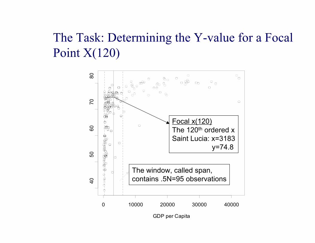
x(120)
Focal x(120) The 120th ordered xSaint Lucia: x=3183 y=74.8
The window, called span,contains .5N=95 observations
The Task: Determining the Y-value for a FocalPoint X(120)

0 10000 20000 30000 40000
0.0
0.2
0.4
0.6
0.8
1.0
GDP per Capita
Tricube K
ern
el W
eig
ht
hxxzii
/)( 0!=
Tricube kernel weights
{ 1||..........)||1(
1||.....................0
33
)( <!
"= zforz
zforT zK
Weights within the Span Can Be Determined by the Tricube Kernel Function

The Y-value at Focal X(120) Is a Weighted Mean
0 10000 20000 30000 40000
40
50
60
70
80
GDP per Capita
Fem
ale
Expecta
tion o
f Life
Weighted mean = 71.11301
Country Life Exp. GDP Z Weight
Poland 75.7 3058 1.3158 0
Lebanon 71.7 3114 0.7263 0.23
Saint.Lucia 74.8 3183 0 1.00
South.Africa 68.3 3230 0.4947 0.68
Slovakia 75.8 3266 0.8737 0.04
Venezuela 75.7 3496 3.2947 0
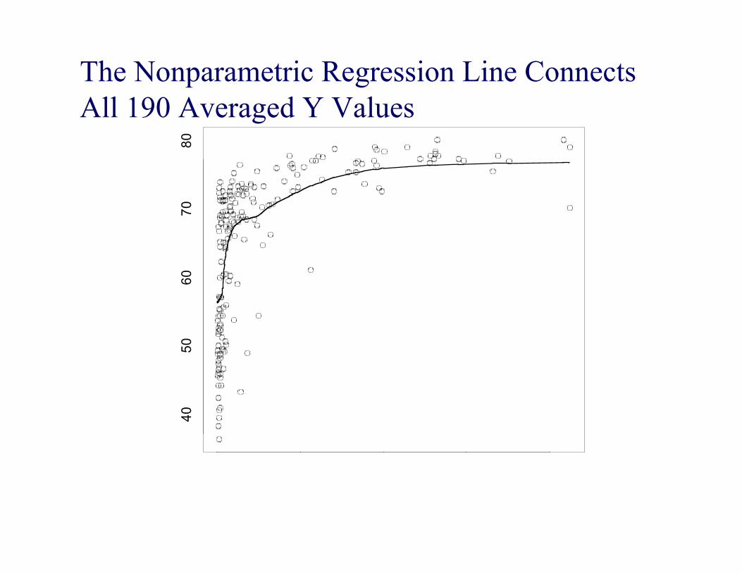
The Nonparametric Regression Line Connects All 190 Averaged Y Values
0 10000 20000 30000 40000
40
50
60
70
80
GDP per Capita
Fem
ale
Expecta
tion o
f Life
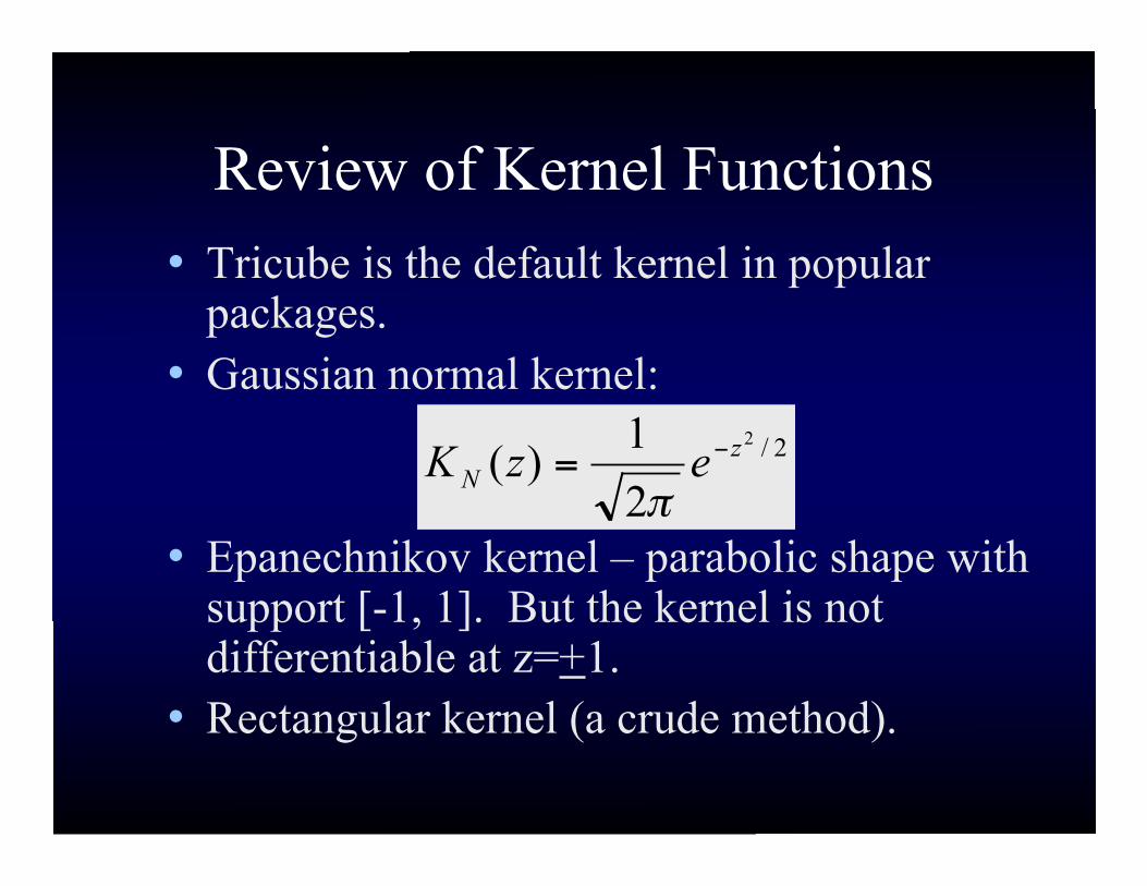
Review of Kernel Functions• Tricube is the default kernel in popular
packages.• Gaussian normal kernel:
• Epanechnikov kernel – parabolic shape withsupport [-1, 1]. But the kernel is notdifferentiable at z=+1.
• Rectangular kernel (a crude method).
2/2
2
1)( z
NezK!
="

Local Linear Regression(Also known as lowess or loess )
• A more sophisticated way to calculate the Yvalues. Instead of constructing weightedaverage, it aims to construct a smooth locallinear regression with estimated β0 and β1 thatminimizes:
where K(.) is a kernel function, typicallytricube.
)()]([1
02
010!"
"""n
i
ii
h
xxKxxY ##
0 10000 20000 30000 40000
40
50
60
70
80
GDP per Capita
Fem
ale
Expecta
tion o
f Life
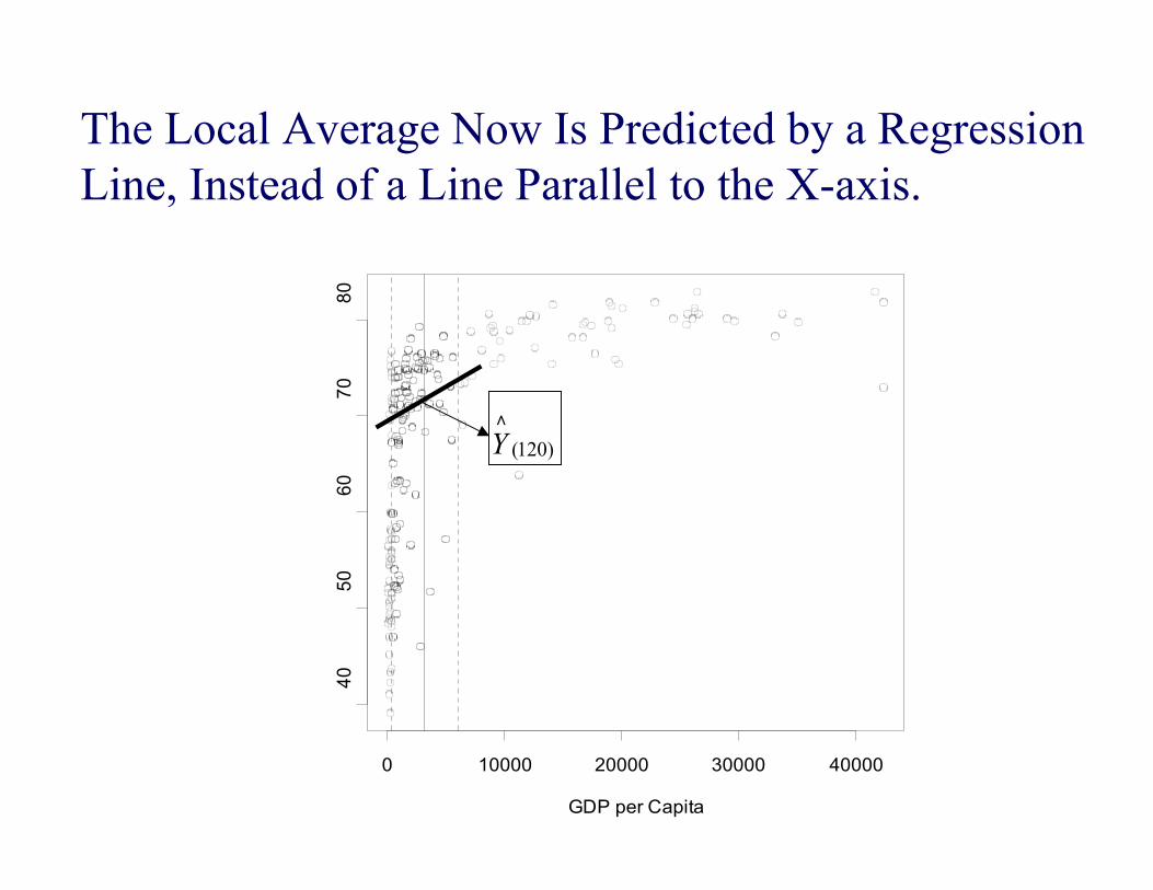
x(120)
)120(Y
!
The Local Average Now Is Predicted by a RegressionLine, Instead of a Line Parallel to the X-axis.

Asymptotic Properties of lowess• Fan (1992, 1993) demonstrated advantages of
lowess over more standard kernel estimators. Heproved that lowess has nice sampling properties andhigh minimax efficiency.
• In Heckman’s works prior to 1997, he and his co-authors used the kernel weights. But since 1997 theyhave used lowess.
• In practice it’s fairly complicated to program theasymptotic properties. No software packagesprovide estimation of the S.E. for lowess. Inpractice, one uses S.E. estimated by bootstrapping.

Bootstrap Statistics Inference (1)• It allows the user to make inferences without making
strong distributional assumptions and without the need foranalytic formulas for the sampling distribution’sparameters.
• Basic idea: treat the sample as if it is the population, andapply Monte Carlo sampling to generate an empiricalestimate of the statistic’s sampling distribution. This isdone by drawing a large number of “resamples” of size nfrom this original sample randomly with replacement.
• A closely related idea is the Jackknife: “drop one out”.That is, it systematically drops out subsets of the data oneat a time and assesses the variation in the samplingdistribution of the statistics of interest.
Bootstrap Statistics Inference (2)• After obtaining estimated standard error (i.e., the standard
deviation of the sampling distribution), one can calculate95 % confidence interval using one of the following threemethods:
Normal approximation method Percentile method Bias-corrected (BC) method
• The BC method is popular.
Finite-Sample Properties of lowess
The finite-sample properties of lowess have beenexamined just recently (Frolich, 2004). Twopractical implications:
1. Choose optimal bandwidth value.2. Trimming (i.e., discarding the nonparametric
regression results in regions where thepropensity scores for the nontreated cases aresparse) may not be the best response to thevariance problems. Sensitivity analysistesting different trimming schemes.

Heckman’s Contributions to PSM• Unlike traditional matching, DID uses propensity
scores differentially to calculate weighted meanof counterfactuals. A creative way to useinformation from multiple matches.
• DID uses longitudinal data (i.e., outcome beforeand after intervention).
• By doing this, the estimator is more robust: iteliminates temporarily-invariant sources of biasthat may arise, when program participants andnonparticipants are geographically mismatched orfrom differences in survey questionnaire.

Demonstration of RunningSTATA/PSMATCH2:
Part 2. Heckman’sDifference-in-differences
Method(Link to file “Day1c.doc”)