introduction to probability€¦ · introduction to probability probability plays a key role in the...

Chapter 18

Introduction to Probability

Probability plays a key role in the sciences —”hard” and social —including computer science. Many algorithms rely on randomization. Investigating their correctness and performance requires probability theory. Moreover, computer systems designs, such as memory management, branch prediction, packet routing, and load balancing are based on probabilistic assumptions and analyses. Probability is central as well in related subjects such as information theory, cryptography, artificial intelligence, and game theory. But we’ll start with a more down-to-earth application: getting a prize in a game show.

18.1 Monty Hall

In the September 9, 1990 issue of Parade magazine, the columnist Marilyn vos Savant responded to this letter:

Suppose you’re on a game show, and you’re given the choice of three doors. Behind one door is a car, behind the others, goats. You pick a door, say number 1, and the host, who knows what’s behind the doors, opens another door, say number 3, which has a goat. He says to you, ”Do you want to pick door number 2?” Is it to your advantage to switch your choice of doors?

Craig. F. Whitaker Columbia, MD

The letter describes a situation like one faced by contestants on the 1970’s game show Let’s Make a Deal, hosted by Monty Hall and Carol Merrill. Marilyn replied that the contestant should indeed switch. She explained that if the car was behind either of the two unpicked doors —which is twice as likely as the the car being behind the picked door —the contestant wins by switching. But she soon received a torrent of letters, many from mathematicians, telling her that she was wrong. The problem generated thousands of hours of heated debate.

409

410 CHAPTER 18. INTRODUCTION TO PROBABILITY

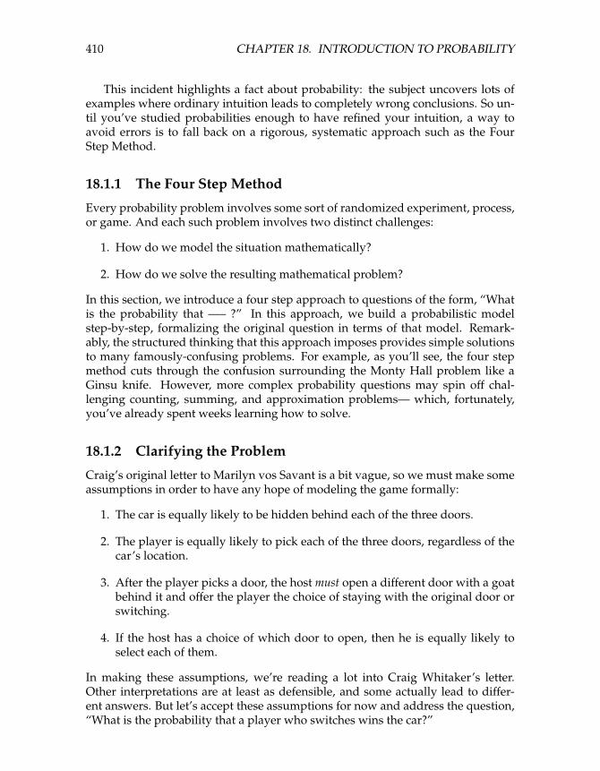
This incident highlights a fact about probability: the subject uncovers lots of examples where ordinary intuition leads to completely wrong conclusions. So until you’ve studied probabilities enough to have refined your intuition, a way to avoid errors is to fall back on a rigorous, systematic approach such as the Four Step Method.

18.1.1 The Four Step Method

Every probability problem involves some sort of randomized experiment, process, or game. And each such problem involves two distinct challenges:

1. How do we model the situation mathematically?

2. How do we solve the resulting mathematical problem?

In this section, we introduce a four step approach to questions of the form, “What is the probability that —– ?” In this approach, we build a probabilistic model step-by-step, formalizing the original question in terms of that model. Remarkably, the structured thinking that this approach imposes provides simple solutions to many famously-confusing problems. For example, as you’ll see, the four step method cuts through the confusion surrounding the Monty Hall problem like a Ginsu knife. However, more complex probability questions may spin off challenging counting, summing, and approximation problems— which, fortunately, you’ve already spent weeks learning how to solve.

18.1.2 Clarifying the Problem

Craig’s original letter to Marilyn vos Savant is a bit vague, so we must make some assumptions in order to have any hope of modeling the game formally:

1. The car is equally likely to be hidden behind each of the three doors.

2. The player is equally likely to pick each of the three doors, regardless of the car’s location.

3. After the player picks a door, the host must open a different door with a goat behind it and offer the player the choice of staying with the original door or switching.

4. If the host has a choice of which door to open, then he is equally likely to select each of them.

In making these assumptions, we’re reading a lot into Craig Whitaker’s letter. Other interpretations are at least as defensible, and some actually lead to different answers. But let’s accept these assumptions for now and address the question, “What is the probability that a player who switches wins the car?”

411 18.1. MONTY HALL

18.1.3 Step 1: Find the Sample Space

Our first objective is to identify all the possible outcomes of the experiment. A typical experiment involves several randomly-determined quantities. For example, the Monty Hall game involves three such quantities:

1. The door concealing the car.

2. The door initially chosen by the player.

3. The door that the host opens to reveal a goat.

Every possible combination of these randomly-determined quantities is called an outcome. The set of all possible outcomes is called the sample space for the experiment.

A tree diagram is a graphical tool that can help us work through the four step approach when the number of outcomes is not too large or the problem is nicely structured. In particular, we can use a tree diagram to help understand the sample space of an experiment. The first randomly-determined quantity in our experiment is the door concealing the prize. We represent this as a tree with three branches:

carlocation

C

A

B

In this diagram, the doors are called A, B, and C instead of 1, 2, and 3 because we’ll be adding a lot of other numbers to the picture later.

Now, for each possible location of the prize, the player could initially choose any of the three doors. We represent this in a second layer added to the tree. Then a third layer represents the possibilities of the final step when the host opens a door to reveal a goat:

� �


carlocation

player’sinitial guess

doorrevealed

C

C

C

A

B

A

B

A

B

C

A

B

C

A

B

A

C

A

CC

B

A

B

outcome

B

(A,A,B)

(A,A,C)

(A,B,C)

(B,A,C)

(B,B,A)

(B,B,C)

(B,C,A)

(C,A,B)

(C,B,A)

(C,C,A)

(C,C,B)

(A,C,B)

Notice that the third layer reflects the fact that the host has either one choice or two, depending on the position of the car and the door initially selected by the player. For example, if the prize is behind door A and the player picks door B, then the host must open door C. However, if the prize is behind door A and the player picks door A, then the host could open either door B or door C.

Now let’s relate this picture to the terms we introduced earlier: the leaves of the tree represent outcomes of the experiment, and the set of all leaves represents the sample space. Thus, for this experiment, the sample space consists of 12 outcomes. For reference, we’ve labeled each outcome with a triple of doors indicating:

(door concealing prize, door initially chosen, door opened to reveal a goat)

In these terms, the sample space is the set:

(A, A,B), (A, A,C), (A, B,C), (A, C,B), (B, A,C), (B, B, A), (B, B, C), (B, C, A), (C, A,B), (C, B,A), (C, C,A), (C, C,B)

The tree diagram has a broader interpretation as well: we can regard the whole experiment as following a path from the root to a leaf, where the branch taken at each stage is “randomly” determined. Keep this interpretation in mind; we’ll use it again later.


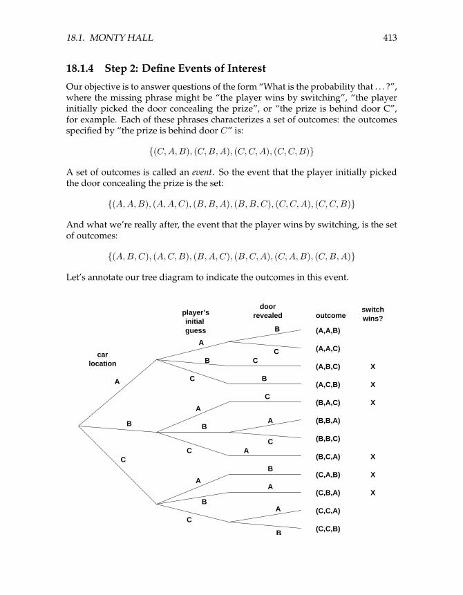
18.1.4 Step 2: Define Events of Interest

Our objective is to answer questions of the form “What is the probability that . . . ?”, where the missing phrase might be “the player wins by switching”, “the player initially picked the door concealing the prize”, or “the prize is behind door C”, for example. Each of these phrases characterizes a set of outcomes: the outcomes specified by “the prize is behind door C” is:

{(C, A,B), (C, B,A), (C, C,A), (C, C,B)}

A set of outcomes is called an event. So the event that the player initially picked the door concealing the prize is the set:

{(A, A,B), (A, A,C), (B, B, A), (B, B, C), (C, C,A), (C, C,B)}

And what we’re really after, the event that the player wins by switching, is the set of outcomes:

{(A, B,C), (A, C,B), (B, A,C), (B, C,A), (C, A,B), (C, B,A)}

Let’s annotate our tree diagram to indicate the outcomes in this event.

carlocation


doorrevealed

switchwins?

C

C

C

A

B

A

B

A

B

C

A

B

C

A

B

A

C

A

CC

B

A

B

outcome

X

X

X

X

X

X

B

(A,A,B)

(A,A,C)

(A,B,C)

(B,A,C)

(B,B,A)

(B,B,C)

(B,C,A)

(C,A,B)

(C,B,A)

(C,C,A)

(C,C,B)

(A,C,B)


Notice that exactly half of the outcomes are marked, meaning that the player wins by switching in half of all outcomes. You might be tempted to conclude that a player who switches wins with probability 1/2. This is wrong. The reason is that these outcomes are not all equally likely, as we’ll see shortly.

18.1.5 Step 3: Determine Outcome Probabilities

So far we’ve enumerated all the possible outcomes of the experiment. Now we must start assessing the likelihood of those outcomes. In particular, the goal of this step is to assign each outcome a probability, indicating the fraction of the time this outcome is expected to occur. The sum of all outcome probabilities must be one, reflecting the fact that there always is an outcome.

Ultimately, outcome probabilities are determined by the phenomenon we’re modeling and thus are not quantities that we can derive mathematically. However, mathematics can help us compute the probability of every outcome based on fewer and more elementary modeling decisions. In particular, we’ll break the task of determining outcome probabilities into two stages.

Step 3a: Assign Edge Probabilities

First, we record a probability on each edge of the tree diagram. These edge-probabilities are determined by the assumptions we made at the outset: that the prize is equally likely to be behind each door, that the player is equally likely to pick each door, and that the host is equally likely to reveal each goat, if he has a choice. Notice that when the host has no choice regarding which door to open, the single branch is assigned probability 1.


carlocation


doorrevealed

switchwins?

C

C

C

A

B

A

B

A

B

C

A

B

C

A

B

A

C

A

CC

1/3

1/3

1/3

1/3

1/3

1/3

1/3

1/3

1/3

1/3

1/3

1/3

1

1

1

1

1

1

1/2 B

1/2

1/2

1/2

A

B

1/2

1/2

outcome

X

X

X

X

X

X

B

(A,A,B)

(A,A,C)

(A,B,C)

(B,A,C)

(B,B,A)

(B,B,C)

(B,C,A)

(C,A,B)

(C,B,A)

(C,C,A)

(C,C,B)

(A,C,B)

Step 3b: Compute Outcome Probabilities

Our next job is to convert edge probabilities into outcome probabilities. This is a purely mechanical process: the probability of an outcome is equal to the product of the edge-probabilities on the path from the root to that outcome. For example, the probability of the topmost outcome, (A, A,B) is

1 1 1 1 = .

3 · 3 · 2 18

There’s an easy, intuitive justification for this rule. As the steps in an experiment progress randomly along a path from the root of the tree to a leaf, the probabilities on the edges indicate how likely the walk is to proceed along each branch. For example, a path starting at the root in our example is equally likely to go down each of the three top-level branches.

Now, how likely is such a walk to arrive at the topmost outcome, (A, A,B)? Well, there is a 1-in-3 chance that a walk would follow the A-branch at the top level, a 1-in-3 chance it would continue along the A-branch at the second level, and 1-in-2 chance it would follow the B-branch at the third level. Thus, it seems that about 1 walk in 18 should arrive at the (A, A,B) leaf, which is precisely the probability we assign it.

Anyway, let’s record all the outcome probabilities in our tree diagram.


carlocation


doorrevealed

switchwins?

C

C

C

A

B

A

B

A

B

C

A

B

C

A

B

A

C

A

CC

1/3

1/3

1/3

1/3

1/3

1/3

1/3

1/3

1/3

1/3

1/3

1/3

1

1

1

1

1

1

1/2 B

1/2

1/2

1/2

A

B

1/2

1/2

outcome

X

X

X

X

X

X

probability

1/18

1/18

1/9

1/9

1/9

1/18

1/18

1/9

1/9

1/9

1/18

1/18

B

(A,A,B)

(A,A,C)

(A,B,C)

(B,A,C)

(B,B,A)

(B,B,C)

(B,C,A)

(C,A,B)

(C,B,A)

(C,C,A)

(C,C,B)

(A,C,B)

Specifying the probability of each outcome amounts to defining a function that maps each outcome to a probability. This function is usually called Pr. In these terms, we’ve just determined that:

1Pr {(A, A,B)} =

181

Pr {(A, A,C)} = 181

Pr {(A, B, C)} = 9

etc.

18.1.6 Step 4: Compute Event Probabilities

We now have a probability for each outcome, but we want to determine the probability of an event which will be the sum of the probabilities of the outcomes in it. The probability of an event, E, is written Pr {E}. For example, the probability of


the event that the player wins by switching is:

Pr {switching wins} = Pr {(A, B,C)} + Pr {(A, C,B)} + Pr {(B, A, C)} +

Pr {(B, C,A)} + Pr {(C, A,B)} + Pr {(C, B,A)}1 1 1 1 1 1

= + + + + +9 9 9 9 9 9 2

= 3

It seems Marilyn’s answer is correct; a player who switches doors wins the car with probability 2/3! In contrast, a player who stays with his or her original door wins with probability 1/3, since staying wins if and only if switching loses.

We’re done with the problem! We didn’t need any appeals to intuition or ingenious analogies. In fact, no mathematics more difficult than adding and multiplying fractions was required. The only hard part was resisting the temptation to leap to an “intuitively obvious” answer.

18.1.7 An Alternative Interpretation of the Monty Hall Problem

Was Marilyn really right? Our analysis suggests she was. But a more accurate conclusion is that her answer is correct provided we accept her interpretation of the question. There is an equally plausible interpretation in which Marilyn’s answer is wrong. Notice that Craig Whitaker’s original letter does not say that the host is required to reveal a goat and offer the player the option to switch, merely that he did these things. In fact, on the Let’s Make a Deal show, Monty Hall sometimes simply opened the door that the contestant picked initially. Therefore, if he wanted to, Monty could give the option of switching only to contestants who picked the correct door initially. In this case, switching never works!

18.1.8 Problems

Class Problems

Problem 18.1.[A Baseball Series]The New York Yankees and the Boston Red Sox are playing a two-out-of-three series. (In other words, they play until one team has won two games. Then that team is declared the overall winner and the series ends.) Assume that the Red Sox win each game with probability 3/5, regardless of the outcomes of previous games.

Answer the questions below using the four step method. You can use the same tree diagram for all three problems. (a) What is the probability that a total of 3 games are played?

(b) What is the probability that the winner of the series loses the first game?

(c) What is the probability that the correct team wins the series?


Problem 18.2. To determine which of two people gets a prize, a coin is flipped twice. If the flips are a Head and then a Tail, the first player wins. If the flips are a Tail and then a Head, the second player wins. However, if both coins land the same way, the flips don’t count and whole the process starts over.

Assume that on each flip, a Head comes up with probability p, regardless of what happened on other flips. Use the four step method to find a simple formula for the probability that the first player wins. What is the probability that neither player wins?

Suggestions: The tree diagram and sample space are infinite, so you’re not going to finish drawing the tree. Try drawing only enough to see a pattern. Summing all the winning outcome probabilities directly is difficult. However, a neat trick solves this problem and many others. Let s be the sum of all winning outcome probabilities in the whole tree. Notice that you can write the sum of all the winning probabilities in certain subtrees as a function of s. Use this observation to write an equation in s and then solve.

Problem 18.3.[The Four-Door Deal]

Let’s see what happens when Let’s Make a Deal is played with four doors. A prize is hidden behind one of the four doors. Then the contestant picks a door. Next, the host opens an unpicked door that has no prize behind it. The contestant is allowed to stick with their original door or to switch to one of the two unopened, unpicked doors. The contestant wins if their final choice is the door hiding the prize.

Use The Four Step Method of Section 18.1 to find the following probabilities. The tree diagram may become awkwardly large, in which case just draw enough of it to make its structure clear.

(a) Contestant Stu, a sanitation engineer from Trenton, New Jersey, stays with his original door. What is the probability that Stu wins the prize?

(b) Contestant Zelda, an alien abduction researcher from Helena, Montana, switches to one of the remaining two doors with equal probability. What is the probability that Zelda wins the prize?

Problem 18.4.[Simulating a fair coin] Suppose you need a fair coin to decide which door tochoose in the 6.042 Monty Hall game. After making everyone in your group emptytheir pockets, all you managed to turn up is some crumpled bubble gum wrappers,a few used tissues, and one penny. However, the penny was from Prof. Meyer’spocket, so it is not safe to assume that it is a fair coin.

How can we use a coin of unknown bias to get the same effect as a fair coin

419 18.2. SET THEORY AND PROBABILITY

of bias 1/2? Draw the tree diagram for your solution, but since it is infinite, draw only enough to see a pattern.

Suggestion: A neat trick allows you to sum all the outcome probabilities that cause you to say ”Heads”: Let s be the sum of all ”Heads” outcome probabilities in the whole tree. Notice that you can write the sum of all the ”Heads” outcome probabilities in certain subtrees as a function of s. Use this observation to write an equation in s and then solve.

Homework Problems

Problem 18.5. I have a deck of 52 regular playing cards, 26 red, 26 black, randomly shuffled. They all lie face down in the deck so that you can’t see them. I will draw a card off the top of the deck and turn it face up so that you can see it and then put it aside. I will continue to turn up cards like this but at some point while there are still cards left in the deck, you have to declare that you want the next card in the deck to be turned up. If that next card turns up black you win and otherwise you lose. Either way, the game is then over. (a) Show that if you take the first card before you have seen any cards, you then

have probability 1/2 of winning the game.

(b) Suppose you don’t take the first card and it turns up red. Show that you have then have a probability of winning the game that is greater than 1/2.

(c) If there are r red cards left in the deck and b black cards, show that the probability of winning in you take the next card is b/(r + b).

(d) Either,

1. come up with a strategy for this game that gives you a probability of winning strictly greater than 1/2 and prove that the strategy works, or,

2. come up with a proof that no such strategy can exist.

18.2 Set Theory and Probability

Let’s abstract what we’ve just done in this Monty Hall example into a general mathematical definition of probability. In the Monty Hall example, there were only finitely many possible outcomes. Other examples in this course will have a countably infinite number of outcomes.

General probability theory deals with uncountable sets like the set of real numbers, but we won’t need these, and sticking to countable sets lets us define the probability of events using sums instead of integrals. It also lets us avoid some distracting technical problems in set theory like the Banach-Tarski “paradox” mentioned in Chapter 5.2.5.

�

�

�

� � �

� �


18.2.1 Probability Spaces

Definition 18.2.1. A countable sample space, S, is a nonempty countable set. An element w ∈ S is called an outcome. A subset of S is called an event.

Definition 18.2.2. A probability function on a sample space, S, is a total function Pr {} : S → R such that

• Pr {w} ≥ 0 for all w ∈ S, and

• Pr {w} = 1. w∈S

The sample space together with a probability function is called a probability space. For any event, E ⊆ S, the probability of E is defined to be the sum of the proba

bilities of the outcomes in E:

Pr {E} ::= Pr {w} . w∈E

An immediate consequence of the definition of event probability is that for disjoint events, E,F ,

Pr {E ∪ F } = Pr {E} + Pr {F } .

This generalizes to a countable number of events. Namely, a collection of sets is pairwise disjoint when no element is in more than one of them —formally, A∩B = ∅for all sets A = B in the collection.

Rule (Sum Rule). If {E0, E1, . . . } is collection of pairwise disjoint events, then

Pr En = Pr {En} . n∈N n∈N

The Sum Rule1 lets us analyze a complicated event by breaking it down into simpler cases. For example, if the probability that a randomly chosen MIT student is native to the United States is 60%, to Canada is 5%, and to Mexico is 5%, then the probability that a random MIT student is native to North America is 70%.

Another consequence of the Sum Rule is that Pr {A} + Pr A = 1, which follows because Pr {S} = 1 and S is the union of the disjoint sets A and A. This equation often comes up in the form

1If you think like a mathematician, you should be wondering if the infinite sum is really necessary. Namely, suppose we had only used finite sums in Definition 18.2.2 instead of sums over all natural numbers. Would this imply the result for infinite sums? It’s hard to find counterexamples, but there are some: it is possible to find a pathological “probability” measure on a sample space satisfying the Sum Rule for finite unions, in which the outcomes w0, w1, . . . each have probability zero, and the probability assigned to any event is either zero or one! So the infinite Sum Rule fails dramatically, since the whole space is of measure one, but it is a union of the outcomes of measure zero.

The construction of such weird examples is beyond the scope of this text. You can learn more about this by taking a course in Set Theory and Logic that covers the topic of “ultrafilters.”

� �


Rule (Complement Rule).

Pr A = 1 − Pr {A} .

Sometimes the easiest way to compute the probability of an event is to compute the probability of its complement and then apply this formula.

Some further basic facts about probability parallel facts about cardinalities of finite sets. In particular:

Pr {B − A} = Pr {B} − Pr {A ∩ B} , (Difference Rule) Pr {A ∪ B} = Pr {A} + Pr {B} − Pr {A ∩ B} , (Inclusion-Exclusion) Pr {A ∪ B} ≤ Pr {A} + Pr {B} . (Boole’s Inequality)

The Difference Rule follows from the Sum Rule because B is the union of the disjoint sets B − A and A ∩ B. Inclusion-Exclusion then follows from the Sum and Difference Rules, because A∪B is the union of the disjoint sets A and B−A. Boole’s inequality is an immediate consequence of Inclusion-Exclusion since probabilities are nonnegative.

The two event Inclusion-Exclusion equation above generalizes to n events in the same way as the corresponding Inclusion-Exclusion rule for n sets. Boole’s inequality also generalizes to

Pr {E1 ∪ · · · ∪ En} ≤ Pr {E1} + · · · + Pr {En} . (Union Bound)

This simple Union Bound is actually useful in many calculations. For example, suppose that Ei is the event that the i-th critical component in a spacecraft fails. Then E1 ∪· · ·∪En is the event that some critical component fails. The Union Bound can give an adequate upper bound on this vital probability.

Similarly, the Difference Rule implies that

If A ⊆ B, then Pr {A} ≤ Pr {B} . (Monotonicity)

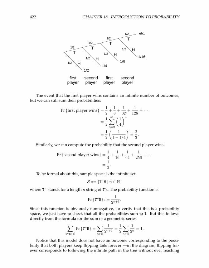
18.2.2 An Infinite Sample Space

Suppose two players take turns flipping a fair coin. Whoever flips heads first is declared the winner. What is the probability that the first player wins? A tree diagram for this problem is shown below:

�

� �


1/21/2

1/21/2

1/21/2

1/21/2

etc.

HH

HHT

TT

T

firstplayer

secondplayer

firstplayer

secondplayer

1/21/4

1/81/16

The event that the first player wins contains an infinite number of outcomes, but we can still sum their probabilities:

1 1 1 1Pr {first player wins} = + + + +

2 8 32 128 · · ·

1 ∞ �

1�n

= 2 4

n=0

1 1 2 = = .

2 1 − 1/4 3

Similarly, we can compute the probability that the second player wins:

1 1 1 1Pr {second player wins} = + + + +

4 16 64 256 · · ·

1 = .

3

To be formal about this, sample space is the infinite set

S ::= {TnH | n ∈ N}

where Tn stands for a length n string of T’s. The probability function is

1Pr {TnH} ::= .

2n+1

Since this function is obviously nonnegative, To verify that this is a probability space, we just have to check that all the probabilities sum to 1. But this follows directly from the formula for the sum of a geometric series: � � 1 1 � 1

Pr {TnH} = = = 1.2n+1 2 2n

TnH∈S n∈N n∈N

Notice that this model does not have an outcome corresponding to the possibility that both players keep flipping tails forever —in the diagram, flipping forever corresponds to following the infinite path in the tree without ever reaching


a leaf/outcome. If leaving this possibility out of the model bothers you, you’re welcome to fix it by adding another outcome, wforever, to indicate that that’s what happened. Of course since the probabililities of the other outcomes already sum to 1, you have to define the probability of wforever to be 0. Now outcomes with probability zero will have no impact on our calculations, so there’s no harm in adding it in if it makes you happier. On the other hand, there’s also no harm in simply leaving it out as we did, since it has no impact.

The mathematical machinery we’ve developed is adequate to model and analyze many interesting probability problems with infinite sample spaces. However, some intricate infinite processes require uncountable sample spaces along with more powerful (and more complex) measure-theoretic notions of probability. For example, if we generate an infinite sequence of random bits b1, b2, b3, . . ., then what is the probability that

b1 b2 b3+ + +21 22 23

· · ·

is a rational number? Fortunately, we won’t have any need to worry about such things.

18.2.3 Problems

Class Problems

Problem 18.6. Suppose there is a system with n components, and we know from past experience that any particular component will fail in a given year with probability p. That is, letting Fi be the event that the ith component fails within one year, we have

Pr {Fi} = p

for 1 ≤ i ≤ n. The system will fail if any one of its components fails. What can we say about the probability that the system will fail within one year?

Let F be the event that the system fails within one year. Without any additional assumptions, we can’t get an exact answer for Pr {F }. However, we can give useful upper and lower bounds, namely,

p ≤ Pr {F } ≤ np. (18.1)

We may as well assume p < 1/n, since the upper bound is trivial otherwise. For example, if n = 100 and p = 10−5, we conclude that there is at most one chance in 1000 of system failure within a year and at least one chance in 100,000.

Let’s model this situation with the sample space S ::= P({1, . . . , n}) whose outcomes are subsets of positive integers ≤ n, where s ∈ S corresponds to the indices of exactly those components that fail within one year. For example, {2, 5} is the outcome that the second and fifth components failed within a year and none of the other components failed. So the outcome that the system did not fail corresponds to the emptyset, ∅.

� �

�


(a) Show that the probability that the system fails could be as small as p by describing appropriate probabilities for the outcomes. Make sure to verify that the sum of your outcome probabilities is 1.

(b) Show that the probability that the system fails could actually be as large as np by describing appropriate probabilities for the outcomes. Make sure to verify that the sum of your outcome probabilities is 1.

(c) Prove inequality (18.1).

Problem 18.7. Here are some handy rules for reasoning about probabilities that all follow directly from the Disjoint Sum Rule in the Appendix. Prove them.

Pr {A − B} = Pr {A} − Pr {A ∩ B} (Difference Rule)

Pr A = 1 − Pr {A} (Complement Rule)

Pr {A ∪ B} = Pr {A} + Pr {B} − Pr {A ∩ B} (Inclusion-Exclusion)

Pr {A ∪ B} ≤ Pr {A} + Pr {B} . (2-event Union Bound)

If A ⊆ B, then Pr {A} ≤ Pr {B} . (Monotonicity)

Problem 18.8. Suppose Pr {} : S → [0, 1] is a probability function on a sample space, S , and let B be an event such that Pr {B} > 0. Define a function PrB {·} on events outcomes w ∈ S by the rule:

PrB {w} ::= Pr {w} / Pr {B} if w ∈ B,

(18.2)0 if w /∈ B.

(a) Prove that PrB {·} is also a probability function on S according to Definition 18.2.2.

(b) Prove that Pr {A ∩ B}

PrB {A} = Pr {B}

for all A ⊆ S.

425 18.3. CONDITIONAL PROBABILITY

18.3 Conditional Probability

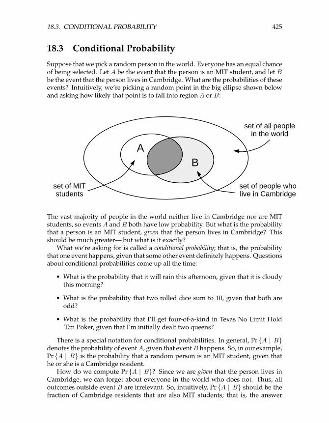
Suppose that we pick a random person in the world. Everyone has an equal chance of being selected. Let A be the event that the person is an MIT student, and let B be the event that the person lives in Cambridge. What are the probabilities of these events? Intuitively, we’re picking a random point in the big ellipse shown below and asking how likely that point is to fall into region A or B:

AB

set of all peoplein the world

set of people wholive in Cambridge

set of MITstudents

The vast majority of people in the world neither live in Cambridge nor are MIT students, so events A and B both have low probability. But what is the probability that a person is an MIT student, given that the person lives in Cambridge? This should be much greater— but what is it exactly?

What we’re asking for is called a conditional probability; that is, the probability that one event happens, given that some other event definitely happens. Questions about conditional probabilities come up all the time:

• What is the probability that it will rain this afternoon, given that it is cloudy this morning?

• What is the probability that two rolled dice sum to 10, given that both are odd?

• What is the probability that I’ll get four-of-a-kind in Texas No Limit Hold ’Em Poker, given that I’m initially dealt two queens?

There is a special notation for conditional probabilities. In general, Pr {A | B}denotes the probability of event A, given that event B happens. So, in our example, Pr {A | B} is the probability that a random person is an MIT student, given that he or she is a Cambridge resident.

How do we compute Pr {A | B}? Since we are given that the person lives in Cambridge, we can forget about everyone in the world who does not. Thus, all outcomes outside event B are irrelevant. So, intuitively, Pr {A | B} should be the fraction of Cambridge residents that are also MIT students; that is, the answer


should be the probability that the person is in set A ∩ B (darkly shaded) divided by the probability that the person is in set B (lightly shaded). This motivates the definition of conditional probability:

Definition 18.3.1.

Pr {A ∩ B}Pr {A | B} ::=

Pr {B}

If Pr {B} = 0, then the conditional probability Pr {A | B} is undefined. Pure probability is often counterintuitive, but conditional probability is worse!

Conditioning can subtly alter probabilities and produce unexpected results in randomized algorithms and computer systems as well as in betting games. Yet, the mathematical definition of conditional probability given above is very simple and should give you no trouble— provided you rely on formal reasoning and not intuition.

18.3.1 The “Halting Problem”

The Halting Problem was the first example of a property that could not be tested by any program. It was introduced by Alan Turing in his seminal 1936 paper. The problem is to determine whether a Turing machine halts on a given . . . yadda yadda yadda . . . what’s much more important, it was the name of the MIT EECS department’s famed C-league hockey team.

In a best-of-three tournament, the Halting Problem wins the first game with probability 1/2. In subsequent games, their probability of winning is determined by the outcome of the previous game. If the Halting Problem won the previous game, then they are invigorated by victory and win the current game with probability 2/3. If they lost the previous game, then they are demoralized by defeat and win the current game with probablity only 1/3. What is the probability that the Halting Problem wins the tournament, given that they win the first game?

This is a question about a conditional probability. Let A be the event that the Halting Problem wins the tournament, and let B be the event that they win the first game. Our goal is then to determine the conditional probability Pr {A | B}.

We can tackle conditional probability questions just like ordinary probability problems: using a tree diagram and the four step method. A complete tree diagram is shown below, followed by an explanation of its construction and use.


2/3

L1/2

W1/2

W 1/3

L2/3

L 1/3

W2/3

LL 1/3

W2/3

W1/3

1st gameoutcome 2nd game

outcome3rd gameoutcome probability

outcome

1/3

1/18

1/9

1/9

1/18

1/3

event B:win the

1st game?

event A:win theseries?

WW

WLW

WLL

LWW

LWL

LL

outcome

Step 1: Find the Sample Space

Each internal vertex in the tree diagram has two children, one corresponding to a win for the Halting Problem (labeled W ) and one corresponding to a loss (labeled L). The complete sample space is:

S = {WW, WLW, WLL, LWW, LWL, LL}

Step 2: Define Events of Interest

The event that the Halting Problem wins the whole tournament is:

T = {WW, WLW, LWW }

And the event that the Halting Problem wins the first game is:

F = {WW, WLW, WLL}

The outcomes in these events are indicated with checkmarks in the tree diagram.

Step 3: Determine Outcome Probabilities

Next, we must assign a probability to each outcome. We begin by labeling edges as specified in the problem statement. Specifically, The Halting Problem has a 1/2 chance of winning the first game, so the two edges leaving the root are each assigned probability 1/2. Other edges are labeled 1/3 or 2/3 based on the outcome


of the preceding game. We then find the probability of each outcome by multiplying all probabilities along the corresponding root-to-leaf path. For example, the probability of outcome WLL is:

1 1 2 1 =

2 · 3 · 3 9

Step 4: Compute Event Probabilities

We can now compute the probability that The Halting Problem wins the tournament, given that they win the first game:

Pr {A ∩ B}Pr {A | B} =

Pr {B}Pr {{WW, WLW }}

= Pr {{WW, WLW, WLL}}

1/3 + 1/18 =

1/3 + 1/18 + 1/9 7

= 9

We’re done! If the Halting Problem wins the first game, then they win the whole tournament with probability 7/9.

18.3.2 Why Tree Diagrams Work

We’ve now settled into a routine of solving probability problems using tree diagrams. But we’ve left a big question unaddressed: what is the mathematical justification behind those funny little pictures? Why do they work?

The answer involves conditional probabilities. In fact, the probabilities that we’ve been recording on the edges of tree diagrams are conditional probabilities. For example, consider the uppermost path in the tree diagram for the Halting Problem, which corresponds to the outcome WW . The first edge is labeled 1/2, which is the probability that the Halting Problem wins the first game. The second edge is labeled 2/3, which is the probability that the Halting Problem wins the second game, given that they won the first— that’s a conditional probability! More generally, on each edge of a tree diagram, we record the probability that the experiment proceeds along that path, given that it reaches the parent vertex.

So we’ve been using conditional probabilities all along. But why can we multiply edge probabilities to get outcome probabilities? For example, we concluded that:

1 2Pr {WW } =

2 · 3

1 =

3


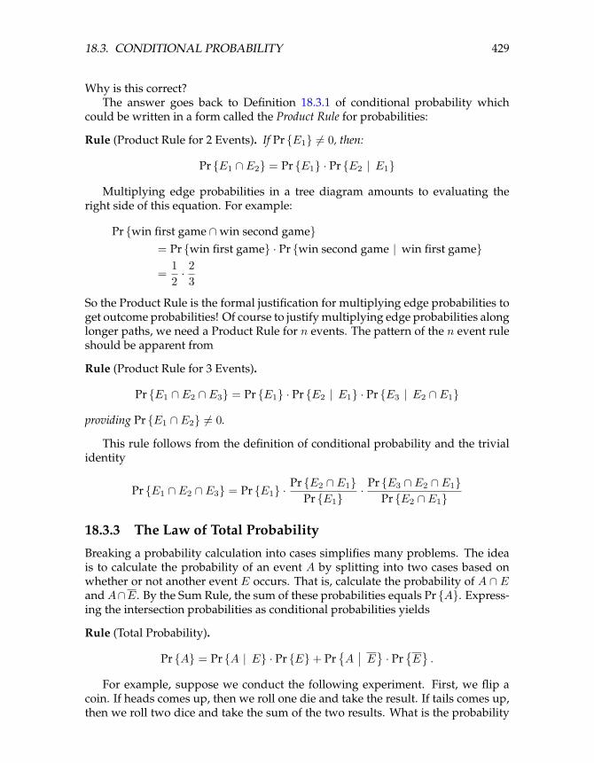
Why is this correct? The answer goes back to Definition 18.3.1 of conditional probability which

could be written in a form called the Product Rule for probabilities:

Rule (Product Rule for 2 Events). If Pr {E1} = 0� , then:

Pr {E1 ∩ E2} = Pr {E1} · Pr {E2 | E1}

Multiplying edge probabilities in a tree diagram amounts to evaluating the right side of this equation. For example:

Pr {win first game ∩ win second game} = Pr {win first game} · Pr {win second game | win first game}

1 2 =

2 · 3

So the Product Rule is the formal justification for multiplying edge probabilities to get outcome probabilities! Of course to justify multiplying edge probabilities along longer paths, we need a Product Rule for n events. The pattern of the n event rule should be apparent from

Rule (Product Rule for 3 Events).

Pr {E1 ∩ E2 ∩ E3} = Pr {E1} · Pr {E2 | E1} · Pr {E3 | E2 ∩ E1}

providing Pr {E1 ∩ E2} = 0� .

This rule follows from the definition of conditional probability and the trivial identity

Pr {E2 ∩ E1} Pr {E3 ∩ E2 ∩ E1}Pr {E1 ∩ E2 ∩ E3} = Pr {E1} · Pr {E1}·

Pr {E2 ∩ E1}

18.3.3 The Law of Total Probability

Breaking a probability calculation into cases simplifies many problems. The idea is to calculate the probability of an event A by splitting into two cases based on whether or not another event E occurs. That is, calculate the probability of A ∩ E and A ∩ E. By the Sum Rule, the sum of these probabilities equals Pr {A}. Expressing the intersection probabilities as conditional probabilities yields

Rule (Total Probability). � � � � � Pr {A} = Pr {A | E} · Pr {E} + Pr A � E · Pr E .

For example, suppose we conduct the following experiment. First, we flip a coin. If heads comes up, then we roll one die and take the result. If tails comes up, then we roll two dice and take the sum of the two results. What is the probability

� �

� �

�


that this process yields a 2? Let E be the event that the coin comes up heads, and let A be the event that we get a 2 overall. Assuming that the coin is fair, Pr {E} = Pr E = 1/2. There are now two cases. If we flip heads, then we roll a 2 on a single die with probabilty Pr {A | E} = 1/6. �On the other hand, if we flip tails, then we get a sum of 2 on two dice with probability Pr A � E = 1/36. Therefore, the probability that the whole process yields a 2 is

1 1 1 1 7Pr {A} = + = .

2 · 6 2

· 36 72

There is also a form of the rule to handle more than two cases.

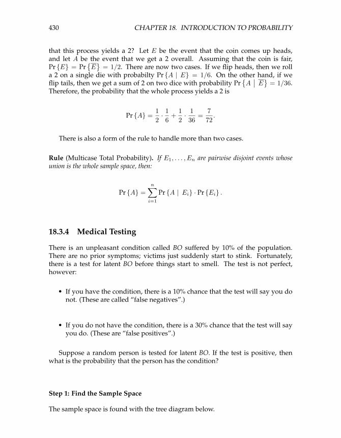
Rule (Multicase Total Probability). If E1, . . . , En are pairwise disjoint events whose union is the whole sample space, then:

n

Pr {A} = Pr {A | Ei} · Pr {Ei} . i=1

18.3.4 Medical Testing

There is an unpleasant condition called BO suffered by 10% of the population. There are no prior symptoms; victims just suddenly start to stink. Fortunately, there is a test for latent BO before things start to smell. The test is not perfect, however:

• If you have the condition, there is a 10% chance that the test will say you do not. (These are called “false negatives”.)

• If you do not have the condition, there is a 30% chance that the test will say you do. (These are “false positives”.)

Suppose a random person is tested for latent BO. If the test is positive, then what is the probability that the person has the condition?

Step 1: Find the Sample Space

The sample space is found with the tree diagram below.


personhas BO?

test result outcomeprobability event A B?

yes

no

pos

neg

pos

neg

.1

.9

.9

.1

.3

.7

.09

.01

.27

.63event A: event B:

hasBO?

testpositive?

Step 2: Define Events of Interest

Let A be the event that the person has BO. Let B be the event that the test was positive. The outcomes in each event are marked in the tree diagram. We want to find Pr {A | B}, the probability that a person has BO, given that the test was positive.

Step 3: Find Outcome Probabilities

First, we assign probabilities to edges. These probabilities are drawn directly from the problem statement. By the Product Rule, the probability of an outcome is the product of the probabilities on the corresponding root-to-leaf path. All probabilities are shown in the figure.

Step 4: Compute Event Probabilities

p

Pr {A B} = Pr {A ∩ B}|

Pr {B}0.09

= 0.09 + 0.27 1

= 4

If you test positive, then there is only a 25% chance that you have the condition!


This answer is initially surprising, but makes sense on reflection. There are two ways you could test positive. First, it could be that you are sick and the test is correct. Second, it could be that you are healthy and the test is incorrect. The problem is that almost everyone is healthy; therefore, most of the positive results arise from incorrect tests of healthy people!

We can also compute the probability that the test is correct for a random person. This event consists of two outcomes. The person could be sick and the test positive (probability 0.09), or the person could be healthy and the test negative (probability 0.63). Therefore, the test is correct with probability 0.09 + 0.63 = 0.72. This is a relief; the test is correct almost three-quarters of the time.

But wait! There is a simple way to make the test correct 90% of the time: always return a negative result! This “test” gives the right answer for all healthy people and the wrong answer only for the 10% that actually have the condition. The best strategy is to completely ignore the test result!

There is a similar paradox in weather forecasting. During winter, almost all days in Boston are wet and overcast. Predicting miserable weather every day may be more accurate than really trying to get it right!

18.3.5 Conditional Identities

The probability rules above extend to probabilities conditioned on the same event. For example, the Inclusion-Exclusion formula for two sets holds when all probabilities are conditioned on an event C:

Pr {A ∪ B | C} = Pr {A | C} + Pr {B | C} − Pr {A ∩ B | C} .

This follows from the fact that if Pr {C} = 0 � and we define

PrC {A} ::= Pr {A | C}

then PrC {} satisfies the definition of being probability function. It is important not to mix up events before and after the conditioning bar. For

example, the following is not a valid identity:

False Claim.

Pr {A | B ∪ C} = Pr {A | B} + Pr {A | C} − Pr {A | B ∩ C} . (18.3)

A counterexample is shown below. In this case, Pr {A | B} = 1, Pr {A | C} = 1, and Pr {A | B ∪ C} = 1. However, since 1 =� 1 + 1, the equation above does not hold.


sample space

A

BC

So you’re convinced that this equation is false in general, right? Let’s see if you really believe that.

18.3.6 Discrimination Lawsuit

Several years ago there was a sex discrimination lawsuit against Berkeley. A female professor was denied tenure, allegedly because she was a woman. She argued that in every one of Berkeley’s 22 departments, the percentage of male applicants accepted was greater than the percentage of female applicants accepted. This sounds very suspicious!

However, Berkeley’s lawyers argued that across the whole university the percentage of male tenure applicants accepted was actually lower than the percentage of female applicants accepted. This suggests that if there was any sex discrimination, then it was against men! Surely, at least one party in the dispute must be lying.

Let’s simplify the problem and express both arguments in terms of conditional probabilities. Suppose that there are only two departments, EE and CS, and consider the experiment where we pick a random applicant. Define the following events:

• Let A be the event that the applicant is accepted.

• Let FEE the event that the applicant is a female applying to EE.

• Let FCS the event that the applicant is a female applying to CS.

• Let MEE the event that the applicant is a male applying to EE.

• Let MCS the event that the applicant is a male applying to CS.

Assume that all applicants are either male or female, and that no applicant applied to both departments. That is, the events FEE , FCS , MEE , and MCS are all disjoint.

In these terms, the plaintiff is make the following argument:

Pr {A | FEE } < Pr {A | MEE }Pr {A | FCS } < Pr {A | MCS }


That is, in both departments, the probability that a woman is accepted for tenure is less than the probability that a man is accepted. The university retorts that overall a woman applicant is more likely to be accepted than a man:

Pr {A | FEE ∪ FCS } > Pr {A | MEE ∪ MCS }

It is easy to believe that these two positions are contradictory. In fact, we might even try to prove this by adding the plaintiff’s two inequalities and then arguing as follows:

Pr {A | FEE } + Pr {A | FCS } < Pr {A | MEE } + Pr {A | MCS } ⇒ Pr {A | FEE ∪ FCS } < Pr {A | MEE ∪ MCS }

The second line exactly contradicts the university’s position! But there is a big problem with this argument; the second inequality follows from the first only if we accept the false identity (18.3). This argument is bogus! Maybe the two parties do not hold contradictory positions after all!

In fact, the table below shows a set of application statistics for which the assertions of both the plaintiff and the university hold:

CS 0 females accepted, 1 applied 0% 50 males accepted, 100 applied 50%

EE 70 females accepted, 100 applied 70% 1 male accepted, 1 applied 100%

Overall 70 females accepted, 101 applied ≈ 70% 51 males accepted, 101 applied ≈ 51%

In this case, a higher percentage of males were accepted in both departments, but overall a higher percentage of females were accepted! Bizarre!

18.3.7 A Posteriori Probabilities

Suppose that we turn the hockey question around: what is the probability that the Halting Problem won their first game, given that they won the series?

This seems like an absurd question! After all, if the Halting Problem won the series, then the winner of the first game has already been determined. Therefore, who won the first game is a question of fact, not a question of probability. However, our mathematical theory of probability contains no notion of one event preceding another— there is no notion of time at all. Therefore, from a mathematical perspective, this is a perfectly valid question. And this is also a meaningful question from a practical perspective. Suppose that you’re told that the Halting Problem won the series, but not told the results of individual games. Then, from your perspective, it makes perfect sense to wonder how likely it is that The Halting Problem won the first game.

A conditional probability Pr {B | A} is called a posteriori if event B precedes event A in time. Here are some other examples of a posteriori probabilities:

�


• The probability it was cloudy this morning, given that it rained in the afternoon.

• The probability that I was initially dealt two queens in Texas No Limit Hold ’Em poker, given that I eventually got four-of-a-kind.

Mathematically, a posteriori probabilities are no different from ordinary probabilities; the distinction is only at a higher, philosophical level. Our only reason for drawing attention to them is to say, “Don’t let them rattle you.”

Let’s return to the original problem. The probability that the Halting Problem won their first game, given that they won the series is Pr {B | A}. We can compute this using the definition of conditional probability and our earlier tree diagram:

Pr {B A} = Pr {B ∩ A}|

Pr {A}1/3 + 1/18

= 1/3 + 1/18 + 1/9 7

= 9

This answer is suspicious! In the preceding section, we showed that Pr {A | B}was also 7/9. Could it be true that Pr {A | B} = Pr {B | A} in general? Some reflection suggests this is unlikely. For example, the probability that I feel uneasy, given that I was abducted by aliens, is pretty large. But the probability that I was abducted by aliens, given that I feel uneasy, is rather small.

Let’s work out the general conditions under which Pr {A | B} = Pr {B | A}. By the definition of conditional probability, this equation holds if an only if:

Pr {A ∩ B} Pr {A ∩ B}=

Pr {B} Pr {A}

This equation, in turn, holds only if the denominators are equal or the numerator is 0:

Pr {B} = Pr {A} or Pr {A ∩ B} = 0

The former condition holds in the hockey example; the probability that the Halting Problem wins the series (event A) is equal to the probability that it wins the first game (event B). In fact, both probabilities are 1/2.

Such pairs of probabilities are related by Bayes’ Rule:

Theorem 18.3.2 (Bayes’ Rule). If Pr {A} and Pr {B} are nonzero, then:

Pr {A | B} · Pr {B} = Pr {B (18.4)

Pr {A}| A}

Proof. When Pr {A} and Pr {B} are nonzero, we have

Pr {A | B} · Pr {B} = Pr {A ∩ B} = Pr {B | A} · Pr {A}

by definition of conditional probability. Dividing by Pr {A} gives (18.4).


In the hockey problem, the probability that the Halting Problem wins the first game is 1/2 and so is the probability that the Halting Problem wins the series. Therefore, Pr {A} = Pr {B} = 1/2. This, together with Bayes’ Rule, explains why Pr {A | B} and Pr {B | A} turned out to be equal in the hockey example.

18.3.8 Problems

Practice Problems

Problem 18.9. Dirty Harry places two bullets in the six-shell cylinder of his revolver. He gives the cylinder a random spin and says “Feeling lucky?” as he holds the gun against your heart. (a) What is the probability that you will get shot if he pulls the trigger?

(b) Suppose he pulls the trigger and you don’t get shot. What is the probability that you will get shot if he pulls the trigger a second time?

(c) Suppose you noticed that he placed the two shells next to each other in the cylinder. How does this change the answers to the previous two questions?

Class Problems

Problem 18.10. There are two decks of cards. One is complete, but the other is missing the ace of spades. Suppose you pick one of the two decks with equal probability and then select a card from that deck uniformly at random. What is the probability that you picked the complete deck, given that you selected the eight of hearts? Use the four-step method and a tree diagram.

Problem 18.11. There are three prisoners in a maximum-security prison for fictional villains: the Evil Wizard Voldemort, the Dark Lord Sauron, and Little Bunny Foo-Foo. The parole board has declared that it will release two of the three, chosen uniformly at random, but has not yet released their names. Naturally, Sauron figures that he will be released to his home in Mordor, where the shadows lie, with probability 2/3.

A guard offers to tell Sauron the name of one of the other prisoners who will be released (either Voldemort or Foo-Foo). Sauron knows the guard to be a truthful fellow. However, Sauron declines this offer. He reasons that if the guard says, for example, “Little Bunny Foo-Foo will be released”, then his own probability of release will drop to 1/2. This is because he will then know that either he or Voldemort will also be released, and these two events are equally likely.

Using a tree diagram and the four-step method, either prove that the Dark Lord Sauron has reasoned correctly or prove that he is wrong. Assume that if the guard


has a choice of naming either Voldemort or Foo-Foo (because both are to be released), then he names one of the two uniformly at random.

Homework Problems

Problem 18.12. There is a course —not 6.042, naturally —in which 10% of the assigned problems contain errors. If you ask a TA whether a problem has an error, then he or she will answer correctly 80% of the time. This 80% accuracy holds regardless of whether or not a problem has an error. Likewise when you ask a lecturer, but with only 75% accuracy.

We formulate this as an experiment of choosing one problem randomly and asking a particular TA and Lecturer about it. Define the following events:

E ::= “the problem has an error,”T ::= “the TA says the problem has an error,”L ::= “the lecturer says the problem has an error.”

(a) Translate the description above into a precise set of equations involving conditional probabilities among the events E, T , and L

(b) Suppose you have doubts about a problem and ask a TA about it, and she tells you that the problem is correct. To double-check, you ask a lecturer, who says that the problem has an error. Assuming that the correctness of the lecturers’ answer and the TA’s answer are independent of each other, regardless of whether there is an error2, what is the probability that there is an error in the problem?

(c) Is the event that “the TA says that there is an error”, independent of the event that “the lecturer says that there is an error”?

Problem 18.13. (a) Suppose you repeatedly flip a fair coin until you see the sequence HHT or the sequence TTH. What is the probability you will see HHT first? Hint: Symmetry between Heads and Tails.

(b) What is the probability you see the sequence HTT before you see the sequence HHT? Hint: Try to find the probability that HHT comes before HTT conditioning on whether you first toss an H or a T. The answer is not 1/2.

Problem 18.14. A 52-card deck is thoroughly shuffled and you are dealt a hand of 13 cards. (a) If you have one ace, what is the probability that you have a second ace?

2This assumption is questionable: by and large, we would expect the lecturer and the TA’s to spot the same glaring errors and to be fooled by the same subtle ones.


(b) If you have the ace of spades, what is the probability that you have a second ace?

Remarkably, the two answers are different. This problem will test your counting ability!

Problem 18.15. You are organizing a neighborhood census and instruct your census takers to knock on doors and note the sex of any child that answers the knock. Assume that there are two children in a household and that girls and boys are equally likely to be children and to open the door.

A sample space for this experiment has outcomes that are triples whose first element is either B or G for the sex of the elder child, likewise for the second element and the sex of the younger child, and whose third coordinate is E or Y indicating whether the elder child or younger child opened the door. For example, (B, G, Y) is the outcome that the elder child is a boy, the younger child is a girl, and the girl opened the door. (a) Let T be the event that the household has two girls, and O be the event that a

girl opened the door. List the outcomes in T and O.

(b) What is the probability Pr {T | O}, that both children are girls, given that a girl opened the door?

(c) Where is the mistake in the following argument?

If a girl opens the door, then we know that there is at least one girl in the household. The probability that there is at least one girl is

1 − Pr {both children are boys} = 1 − (1/2 × 1/2) = 3/4. (18.5)

So,

Pr {T | there is at least one girl in the household}

= Pr {T ∩ there is at least one girl in the household}

Pr {there is at least one girl in the household}

= Pr {T }

Pr {there is at least one girl in the household}= (1/4)/(3/4) = 1/3.

(18.6)

(18.7)

(18.8)

(18.9)

Therefore, given that a girl opened the door, the probability that there are two girls in the household is 1/3.

18.4 Independence

Suppose that we flip two fair coins simultaneously on opposite sides of a room.Intuitively, the way one coin lands does not affect the way the other coin lands.

�

439 18.4. INDEPENDENCE

The mathematical concept that captures this intuition is called independence:

Definition. Events A and B are independent if and only if:

Pr {A ∩ B} = Pr {A} · Pr {B}

Generally, independence is something you assume in modeling a phenomenon— or wish you could realistically assume. Many useful probability formulas only hold if certain events are independent, so a dash of independence can greatly simplify the analysis of a system.

18.4.1 Examples

Let’s return to the experiment of flipping two fair coins. Let A be the event that the first coin comes up heads, and let B be the event that the second coin is heads. If we assume that A and B are independent, then the probability that both coins come up heads is:

Pr {A ∩ B} = Pr {A} · Pr {B}1 1

= 2 · 2

1 =

4

On the other hand, let C be the event that tomorrow is cloudy and R be the event that tomorrow is rainy. Perhaps Pr {C} = 1/5 and Pr {R} = 1/10 around here. If these events were independent, then we could conclude that the probability of a rainy, cloudy day was quite small:

Pr {R ∩ C} = Pr {R} · Pr {C}1 1

= 5 · 10

1 =

50

Unfortunately, these events are definitely not independent; in particular, every rainy day is cloudy. Thus, the probability of a rainy, cloudy day is actually 1/10.

18.4.2 Working with Independence

There is another way to think about independence that you may find more intuitive. According to the definition, events A and B are independent if and only if Pr {A ∩ B} = Pr {A}·Pr {B}. This equation holds even if Pr {B} = 0, but assuming it is not, we can divide both sides by Pr {B} and use the definition of conditional probability to obtain an alternative formulation of independence:

Proposition. If Pr {B} = 0, then events A and B are independent if and only if

Pr {A | B} = Pr {A} . (18.10)


Equation (18.10) says that events A and B are independent if the probability of A is unaffected by the fact that B happens. In these terms, the two coin tosses of the previous section were independent, because the probability that one coin comes up heads is unaffected by the fact that the other came up heads. Turning to our other example, the probability of clouds in the sky is strongly affected by the fact that it is raining. So, as we noted before, these events are not independent.

Warning: Students sometimes get the idea that disjoint events are independent. The opposite is true: if A ∩ B = ∅, then knowing that A happens means you know that B does not happen. So disjoint events are never independent —unless one of them has probability zero.

18.4.3 Mutual Independence

We have defined what it means for two events to be independent. But how can we talk about independence when there are more than two events? For example, how can we say that the orientations of n coins are all independent of one another?

Events E1, . . . , En are mutually independent if and only if for every subset of the events, the probability of the intersection is the product of the probabilities. In other words, all of the following equations must hold:

Pr {Ei ∩ Ej } = Pr {Ei} · Pr {Ej } for all distinct i, j

Pr {Ei ∩ Ej ∩ Ek} = Pr {Ei} · Pr {Ej } · Pr {Ek} for all distinct i, j, k

Pr {Ei ∩ Ej ∩ Ek ∩ El} = Pr {Ei} · Pr {Ej } · Pr {Ek} · Pr {El} for all distinct i, j, k, l . . .

Pr {E1 ∩ · · · ∩ En} = Pr {E1} · · · Pr {En}

As an example, if we toss 100 fair coins and let Ei be the event that the ith coin lands heads, then we might reasonably assume that E1, . . . , E100 are mutually independent.

18.4.4 Pairwise Independence

The definition of mutual independence seems awfully complicated— there are so many conditions! Here’s an example that illustrates the subtlety of independence when more than two events are involved and the need for all those conditions. Suppose that we flip three fair, mutually-independent coins. Define the following events:

• A1 is the event that coin 1 matches coin 2.



Are A1, A2, A3 mutually independent?

441 18.4. INDEPENDENCE

The sample space for this experiment is:

{HHH, HHT, HTH, HTT, THH, THT, TTH, TTT }

Every outcome has probability (1/2)3 = 1/8 by our assumption that the coins are mutually independent.

To see if events A1, A2, and A3 are mutually independent, we must check a sequence of equalities. It will be helpful first to compute the probability of each event Ai:

Pr {A1} = Pr {HHH} + Pr {HHT } + Pr {TTH} + Pr {TTT }1 1 1 1

= + + +8 8 8 8 1

= 2

By symmetry, Pr {A2} = Pr {A3} = 1/2 as well. Now we can begin checking all the equalities required for mutual independence.

Pr {A1 ∩ A2} = Pr {HHH} + Pr {TTT }1 1

= +8 8 1

= 4 1 1

= 2 · 2

= Pr {A1} Pr {A2}

By symmetry, Pr {A1 ∩ A3} = Pr {A1} · Pr {A3} and Pr {A2 ∩ A3} = Pr {A2} · Pr {A3} must hold also. Finally, we must check one last condition:

Pr {A1 ∩ A2 ∩ A3} = Pr {HHH} + Pr {TTT }1 1

= +8 8 1

= 4

1 = Pr {A1} Pr {A2} Pr {A3} =�

8

The three events A1, A2, and A3 are not mutually independent even though any two of them are independent! This not-quite mutual independence seems weird at first, but it happens. It even generalizes:

Definition 18.4.1. A set A0, A1, . . . of events is k-way independent iff every set of k of these events is mutually independent. The set is pairwise independent iff it is 2-way independent.


So the sets A1, A2, A3 above are pairwise independent, but not mutually independent. Pairwise independence is a much weaker property than mutual independence, but it’s all that’s needed to justify a standard approach to making probabilistic estimates that will come up later.

18.4.5 Problems

Class Problems

Problem 18.16. Suppose that you flip three fair, mutually independent coins. Define the following events:

• Let A be the event that the first coin is heads.

• Let B be the event that the second coin is heads.

• Let C be the event that the third coin is heads.

• Let D be the event that an even number of coins are heads.

(a) Use the four step method to determine the probability space for this experiment and the probability of each of A, B,C, D.

(b) Show that these events are not mutually independent.

(c) Show that they are 3-way independent.

18.5 The Birthday Principle

There are 85 students in a class. What is the probability that some birthday is shared by two people? Comparing 85 students to the 365 possible birthdays, you might guess the probability lies somewhere around 1/4 —but you’d be wrong: the probability that there will be two people in the class with matching birthdays is actually more than 0.9999.

To work this out, we’ll assume that the probability that a randomly chosen student has a given birthday is 1/d, where d = 365 in this case. We’ll also assume that a class is composed of n randomly and independently selected students, with n = 85 in this case. These randomness assumptions are not really true, since more babies are born at certain times of year, and students’ class selections are typically not independent of each other, but simplifying in this way gives us a start on analyzing the problem. More importantly, these assumptions are justifiable in important computer science applications of birthday matching. For example, the birthday matching is a good model for collisions between items randomly inserted into a hash table. So we won’t worry about things like Spring procreation preferences that make January birthdays more common, or about twins’ preferences to take classes together (or not).

� �

� �

443 18.5. THE BIRTHDAY PRINCIPLE

Selecting a sequence of n students for a class yields a sequence of n birthdays. Under the assumptions above, the dn possible birthday sequences are equally likely outcomes. Let’s examine the consequences of this probability model by focussing on the ith and jth elements in a birthday sequence, where 1 ≤ i =� j ≤ n. It makes for a better story if we refer to the ith birthday as “Alice’s” and the jth as “Bob’s.”

Now since Bob’s birthday is assumed to be independent of Alice’s, it follows that whichever of the d birthdays Alice’s happens to be, the probability that Bob has the same birthday 1/d. Next, If we look at two other birthdays —call them “Carol’s” and “Don’s” —then whether Alice and Bob have matching birthdays has nothing to do with whether Carol and Don have matching birthdays. That is, the event that Alice and Bob have matching birthdays is independent of the event that Carol and Don have matching birthdays. In fact, for any set of non-overlapping couples, the events that a couple has matching birthdays are mutually independent.

In fact, it’s pretty clear that the probability that Alice and Bob have matching birthdays remains 1/d whether or not Carol and Alice have matching birthdays. That is, the event that Alice and Bob match is also independent of Alice and Carol matching. In short, the set of all events in which a couple has macthing birthdays is pairwise independent, despite the overlapping couples. This will be important in Chapter 21 because pairwise independence will be enough to justify some conclusions about the expected number of matches. However, it’s obvious that these matching birthday events are not mutually independent, not even 3-way independent: if Alice and Bob match and also Alice and Carol match, then Bob and Carol will match.

We could justify all these assertions of independence routinely using the four step method, but it’s pretty boring, and we’ll skip it.

It turns out that as long as the number of students is noticeably smaller than the number of possible birthdays, we can get a pretty good estimate of the birthday matching probabilities by pretending that the matching events are mutually independent. (An intuitive justification for this is that with only a small number of matching pairs, it’s likely that none of the pairs overlap.) Then the probability of no matching birthdays would be the same as rth power of the probability that a couple does not have matching birthdays, where r ::= n

2 is the number of couples. That is, the probability of no matching birthdays would be

2 )(1 − 1/d)(n

. (18.11)

xUsing the fact that e > 1 + x for all x,3 we would conclude that the probability of no matching birthdays is at most

n 2

e−

d . (18.12)

3This approximation is obtained by truncating the Taylor series e−x = 1 − x + x2/2! − x3/3! + · · · . The approximation e−x ≈ 1 − x is pretty accurate when x is small.


The matching birthday problem fits in here so far as a nice example illustrating pairwise and mutual independence. But it’s actually not hard to justify the bound (18.12) without any pretence or any explicit consideration of independence. Namely, there are d(d − 1)(d − 2) (d − (n − 1)) length n sequences of distinct · · · birthdays. So the probability that everyone has a different birthday is:

d(d − 1)(d − 2) (d − (n − 1))· · · dn

d d − 1 d − 2 d − (n − 1)=

d ·

d ·

d · · ·

d� ��

= 1 − 0 d

1 − 1 d

1 − 2 d · · · 1 −

n − 1 d

0 e−1/d e−2/d e−(n−1)/d< e (since 1 + x < ex)· · · · · n−1

= e−(P i=1 i/d)

= e−(n(n−1)/2d)

= the bound (18.12).

For n = 85 and d = 365, (18.12) is less than 1/17, 000, which means the probability of having some pair of matching birthdays actually is more than 1−1/17, 000 > 0.9999. So it would be pretty astonishing if there were no pair of students in the class with matching birthdays.

For d ≤ n2/2, the probability of no match turns out to be asymptotically equal to the upper bound (18.12). For d = n2/2 in particular, the probability of no match is asymptotically equal to 1/e. This leads to a rule of thumb which is useful in many contexts in computer science:

The Birthday Principle

If there are d days in a year and √

2d people in a room, then the probability that two share a birthday is about 1 − 1/e ≈ 0.632.

For example, the Birthday Principle says that if you have √

2 365 ≈ 27 people· in a room, then the probability that two share a birthday is about 0.632. The actual probability is about 0.626, so the approximation is quite good.

Among other applications, the Birthday Principle famously comes into play as the basis of “birthday attacks” that crack certain cryptographic systems.

MIT OpenCourseWarehttp://ocw.mit.edu

6.042J / 18.062J Mathematics for Computer Science Spring 2010

For information about citing these materials or our Terms of Use, visit: http://ocw.mit.edu/terms.

http://ocw.mit.edu

http://ocw.mit.edu/terms

introduction to probability€¦ · introduction to probability probability plays a key role in the...

Documents