introduction to olin package - bioconductor
TRANSCRIPT

Introduction to OLIN package
Matthias E. FutschikSysBioLab, Universidade do Algarve
URL: http://olin.sysbiolab.eu
October 30, 2018
Contents
1 Overview 1
2 Installation requirements 2
3 Inspection for intensity-dependent and spatial artifacts 2
4 Optimised local intensity-dependent normalisation 54.1 OLIN . . . . . . . . . . . . . . . . . . . . . . . . . . . . . . . . . . . . . . . . . 64.2 OSLIN . . . . . . . . . . . . . . . . . . . . . . . . . . . . . . . . . . . . . . . . . 9
5 Scaling between arrays of a batch 12
6 Statistical assessment of efficiency of normalisation 14
1 Overview
Microarray measurements are affected by a variety of systematic experimental errors limitingthe accuracy of data produced. Two well-known systematic errors for two-colour arrays arethe so-called intensity-dependent and spatial (location-dependent) dye bias. Normalisationaims to correct for systematic errors in microarray data.
The common linear (or global) normalisation method often fails to correct for dye bias asthis bias is usually not linear. Although non-linear normalisation procedures have been ableto reduce the systematic errors, these methods are based on default parameters and leave it tothe user to choose “good” parameters. The optimal adjustment of the normalisation modelsto the data, however, can be crucial for the efficiency of the normalisation process [1].
The OLIN (Optimised Local Intensity-dependent Normalisation) R-package includes twonormalisation schemes based on iterative local regression and model selection. Both schemesaim to correct for intensity- and location-dependent dye bias in microarray data. For modelselection (parameter optimisation), generalized cross-validation (GCV) is used.
Additionally, several procedures to assess the efficiencies of normalisation are implementedin the package.
A graphical user interface for OLIN has been implemented in the package OLINgui, thatis included in the OLINgui package available at the Bioconductor repository.
1

2 Installation requirements
Following software is required to run the OLIN-package:
� R (> 2.0.0). For installation of R, refer to http://www.r-project.org.
� R-packages: methods, stats, locfit. For installation of these add-on packages, refer tohttp://cran.r-project.org.
� Bioconductor packages: Biobase, marray. Refer to http://www.bioconductor.org forinstallation.
If all requirements are fulfilled, the OLIN add-on R-package can be installed. To see how toinstall add-on R-packages on your computer system, start R and type in help(INSTALL). Op-tionally, you may use the R-function install.packages(). Once the OLIN package is installed,you can load the package by
> library(OLIN)
3 Inspection for intensity-dependent and spatial artifacts
Microarray data often contains many systematic errors. Such errors have to be identified andremoved before further data analysis is conducted. The most basic approach for identificationis the visual inspection of MA- and MXY-plots. MA-plots display the logged fold change (M =log2(Ch2)− log2Ch1) with respect to the average logged spot intensity (A = 0.5(log2(Ch1) +log2Ch2)). MXY-plots display M with respect to the corresponding spot location. Morestringent, but also computationally more expensive, are statistical tests presented in section6.
For illustration, we examine a cDNA microarray experiment comparing gene expression intwo colon cancer cell lines (SW480/SW620). The SW480 cell line was derived from a primarytumor, whereas the SW620 cell line was cultured from a lymph node metastasis of the samepatient. Sharing the same genetic background, these cell lines serve as a model of cancerprogression [3]. The comparison was direct i.e. without using a reference sample. cDNAderived from SW480 cells was labeled by Cy3; cDNA derived from SW620 was labeled byCy5. The SW480/620 experiment consisted of four technical replicates. The data is stored asobject of the class marrayRaw (see the documentation for the package marray). The averagelogged spot intensity A and logged fold changes M can be accessed by using the slot accessormethods maA and maM, respectively.
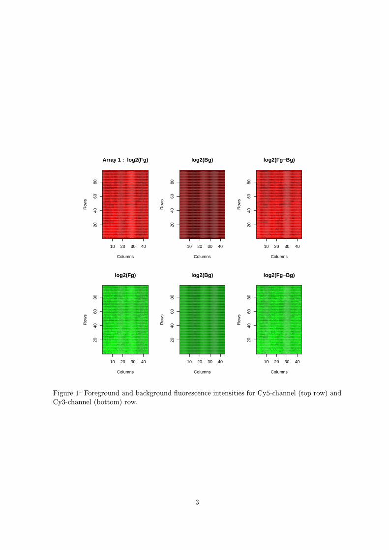
First we want to load the data and inspect the spatial distribution of foreground andbackground intensities in both channels. This can be done using the function fgbg that plotsthe spatial distribution of fore- and background spot intensities for both channels (figure 1):
> data(sw)
> fgbg.visu(sw[,3])
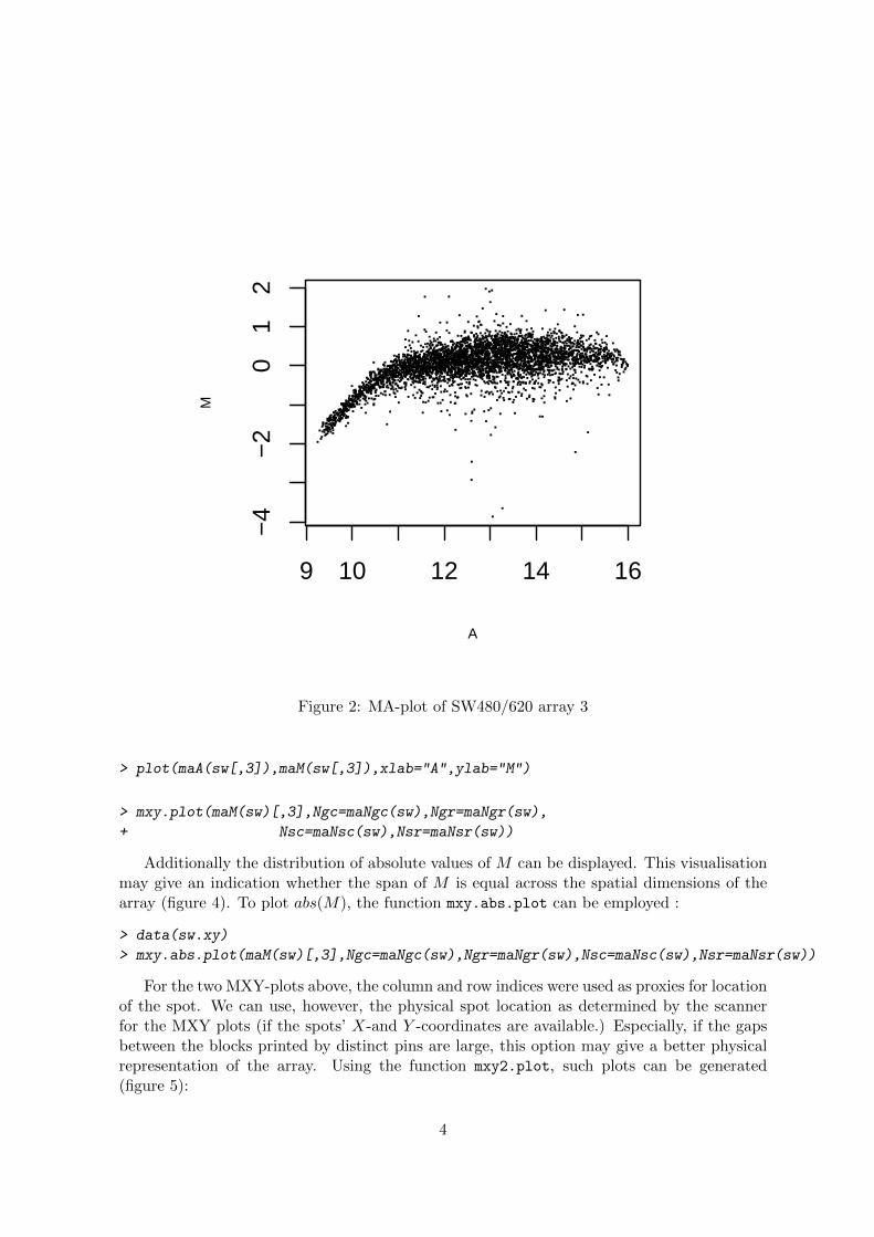
The quantity that we are interested in are the (logged) fold-change M . To inspect anyexisting intensity- or location-dependent bias of M , MA- and MXY-lots can be employed.For MA-lots, the basic plot function can be used (figure 2). MXY-lots can be generated bymxy.plot(figure 3). Note that the function mxy.plot assumes the standard array layout asdefined for marrayRaw/marrayNorm objects.
2
10 20 30 40
2040
6080
Array 1 : log2(Fg)
Columns
Row
s
10 20 30 40
2040
6080
log2(Bg)
Columns
Row
s
10 20 30 4020
4060
80
log2(Fg−Bg)
Columns
Row
s
10 20 30 40
2040
6080
log2(Fg)
Columns
Row
s
10 20 30 40
2040
6080
log2(Bg)
Columns
Row
s
10 20 30 40
2040
6080
log2(Fg−Bg)
Columns
Row
s
Figure 1: Foreground and background fluorescence intensities for Cy5-channel (top row) andCy3-channel (bottom) row.
3
9 10 12 14 16
−4
−2
01
2
A
M
Figure 2: MA-plot of SW480/620 array 3
> plot(maA(sw[,3]),maM(sw[,3]),xlab="A",ylab="M")
> mxy.plot(maM(sw)[,3],Ngc=maNgc(sw),Ngr=maNgr(sw),
+ Nsc=maNsc(sw),Nsr=maNsr(sw))
Additionally the distribution of absolute values of M can be displayed. This visualisationmay give an indication whether the span of M is equal across the spatial dimensions of thearray (figure 4). To plot abs(M), the function mxy.abs.plot can be employed :
> data(sw.xy)
> mxy.abs.plot(maM(sw)[,3],Ngc=maNgc(sw),Ngr=maNgr(sw),Nsc=maNsc(sw),Nsr=maNsr(sw))
For the two MXY-plots above, the column and row indices were used as proxies for locationof the spot. We can use, however, the physical spot location as determined by the scannerfor the MXY plots (if the spots’ X-and Y -coordinates are available.) Especially, if the gapsbetween the blocks printed by distinct pins are large, this option may give a better physicalrepresentation of the array. Using the function mxy2.plot, such plots can be generated(figure 5):
4
10 20 30 40
2040
6080
Columns
Row
s
−1.
0−
0.5
0.0
0.5
1.0
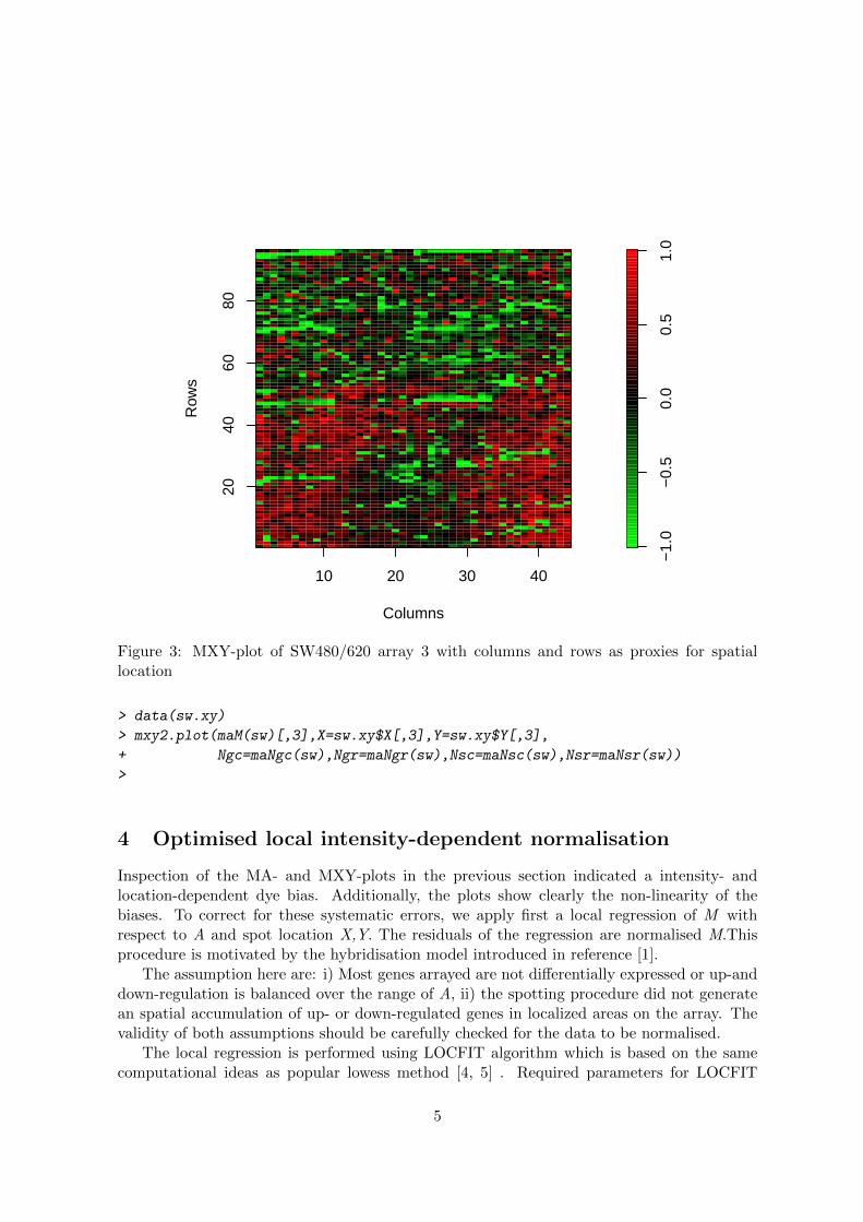
Figure 3: MXY-plot of SW480/620 array 3 with columns and rows as proxies for spatiallocation
> data(sw.xy)
> mxy2.plot(maM(sw)[,3],X=sw.xy$X[,3],Y=sw.xy$Y[,3],
+ Ngc=maNgc(sw),Ngr=maNgr(sw),Nsc=maNsc(sw),Nsr=maNsr(sw))
>
4 Optimised local intensity-dependent normalisation
Inspection of the MA- and MXY-plots in the previous section indicated a intensity- andlocation-dependent dye bias. Additionally, the plots show clearly the non-linearity of thebiases. To correct for these systematic errors, we apply first a local regression of M withrespect to A and spot location X,Y. The residuals of the regression are normalised M.Thisprocedure is motivated by the hybridisation model introduced in reference [1].
The assumption here are: i) Most genes arrayed are not differentially expressed or up-anddown-regulation is balanced over the range of A, ii) the spotting procedure did not generatean spatial accumulation of up- or down-regulated genes in localized areas on the array. Thevalidity of both assumptions should be carefully checked for the data to be normalised.
The local regression is performed using LOCFIT algorithm which is based on the samecomputational ideas as popular lowess method [4, 5] . Required parameters for LOCFIT
5

10 20 30 40
2040
6080
Columns
Row
s
0.0
0.2
0.4
0.6
0.8
1.0
Figure 4: MXY-plot of absolute logged fold changes
are the smoothing parameter α and the scale parameter(s) s for multi-dimensional regression.The parameter α specifies the fraction of points that are included in the neighborhood for localfitting and can have a value between 0 and 1. Larger values lead to smoother fits. The settingof scale parameters s is necessary for a local regression with multiple predictor variables. Thescale parameters s determine the amount of smoothing in one direction compared to the otherdirections.
Choosing accurate regression parameters is crucial for the quality of the normalisation.Too large smoothing parameters, for example, lead to a poor fit where local data featuresare missed and underfitting occurs. If the smoothing parameter is too small, overfitting isproduced and the residuals subsequently underestimated. To optimise the parameter setting,two procedures were developed: OLIN and OSLIN. Both methods are based on iterativelocal regression and parameter selection by GCV. They aim to correct for systematic errorslinked with spot intensity and location. A detailed mathematical description can be found inreference [1].
4.1 OLIN
The OLIN (and OSLIN) are implemented in R by the function olin:
olin(object,X,Y,alpha,iter,OSLIN,scale,weights,genepix,bg.corr,...)
6

0 5000 10000 15000
050
0010
000
1500
0
X
Y
−1.
0−
0.5
0.0
0.5
1.0
Figure 5: MXY plot of SW480/620 array 1
The input arguments are as follows:
object Object of class marrayRaw or marrayNorm containing data of the microarray exper-iment such as spot intensities and array layout for a batch of microarrays. To generatesuch an object, see the marryClasses documentation.
X matrix with x-coordinates of spots. Each column corresponds to one array in the batch.The location is spots detected by scanner is usually found in the output file program ofthe scanning program. If X=NA, the spotted columns on the array are used as proxiesfor the location in x-direction (default)
Y matrix with y-coordinates of spots. If Y=NA, spotted rows on array are used as proxiesfor the location in y-direction (default).
alpha Vector of α parameters that are tested in the GCV procedure. The α parameterdefines the smoothness of fit. The default vector is seq(0.05,1,0.1).
iter Number of iterations in the OLIN or OSLIN procedure. The default value is 3.
OSLIN If OSLIN =TRUE, a subsequent optimised scaling of the range of M across the arrayis performed. The default value is FALSE, i.e. OLIN is performed.
7

scale Vector of scale parameters s that are tested in a GCV procedure. This allows a differentamount of smoothing in Y-direction compared to smoothing in X-direction. The defaultvalues of s are c(0.05,0.1,0.5,1,2,10,20)).
weights Matrix of prior weights of spots for the regression procedures. Spots can be excludedto be used for the local regression by assigning them to zero. If the weight matrix includenegative values, these will be set to zero.For the weights, the weight matrix stored in the maW slot of marrayRaw objects can beused (weights=maW(object)). Defaults is NA resulting in uniform weigths of all spots.
genepix If genepix is set to TRUE, spot weights equal zero or larger are set to one for the localregression whereas negative spot with negative weights are not used for the regression.The argument genepix should be set to TRUE, if weights=maW(object) is set and spotquality weights derived by GenePix are stored in maW(object).
bg.corr backcorrection method (for marrayRaw objects) : none - no background correction,sub - simple background subtraction (default), movingmin - background intensities arefirst averaged over 3x3 grids of neighbouring spots and subsequently substracte, mini-mum - zero or negative intensities after background correction are set equal to half theminimum of positive corrected intensities, edwards- background correction based on log-linear interpolation, or normexp- background correction based on fitting procedure. Forfurther details and references, please refer to to the help page of backgroundCorrect2of the OLIN package or backgroundCorrect of the limma package.
... Further arguments passed to the locfit function.
For illustration, we apply the OLIN scheme to normalise the third array of the SW480/620data set. (Note that the function is not restricted to single slide normalisation but normalisesall arrays in the given marray object.)
> norm.olin <- olin(sw[,3],X=sw.xy$X[,3],Y=sw.xy$Y[,3])
Inspection of the MA- and MXY-plot indicated that OLIN was able to correct for theintensity- as well as the location-dependent dye bias. The residuals are well balanced aroundzero in the MA-plot (figure 6). Similarly, spatial bias is no longer apparent (figure 7). Spotswith positive and negative log ratio M were evenly distributed across the slide. The statisticaltests applied in the next section will confirm these findings.
> plot(maA(norm.olin),maM(norm.olin),main="OLIN",pch=".")
> mxy.plot(maM(norm.olin),Ngc=maNgc(norm.olin),Ngr=maNgr(norm.olin),
+ Nsc=maNsc(norm.olin),Nsr=maNsr(norm.olin),main="OLIN")
>
OLIN is based on an iterative procedure. In most cases, we found that two or threeiterations are already sufficient for normalisation (figure 8).
> norm.olin.1 <- olin(sw[,3],X=sw.xy$X[,3],Y=sw.xy$Y[,3],iter=1)
> norm.olin.2 <- olin(norm.olin.1,X=sw.xy$X[,3],Y=sw.xy$Y[,3],iter=1)
> norm.olin.3 <- olin(norm.olin.2,X=sw.xy$X[,3],Y=sw.xy$Y[,3],iter=1)
> M <- cbind(maM(sw)[,3],maM(norm.olin.1),maM(norm.olin.2),maM(norm.olin.3))
> pairs(M,labels= c("raw","1.Iter.","2.Iter.","3.Iter."))
8

9 11 13 15
−3
−1
1
OLIN
maA(norm.olin)
maM
(nor
m.o
lin)
Figure 6: MA-plot of array normalized by OLIN
4.2 OSLIN
If we can assume that the variability of log ratios M should be equal across the array, localscaling of M can be performed. As in the previous section, the validity of these assumptionshas to be carefully checked for each experiment analyzed. The underlying requirement isagain random spotting of arrayed genes. To apply OSLIN:
> norm.oslin <- olin(sw[,3],X=sw.xy$X[,3],Y=sw.xy$Y[,3],alpha=c(0.1,1,0.1),OSLIN=TRUE)
The local scaling factors are derived by optimized local regression of the absolute log ratioM. The range of regression parameters tested by GCV is [0.1,1] for smoothing parameter. Theresulting MA- and MXY-plots for slide 3 are presented in figures 9 and 10.. The variabilityof log ratios M appears to be even across the array.
> plot(maA(norm.oslin),maM(norm.oslin),main="OSLIN",pch=".")
> mxy.plot(maM(norm.oslin),Ngc=maNgc(norm.oslin),Ngr=maNgr(norm.oslin),
+ Nsc=maNsc(norm.oslin),Nsr=maNsr(norm.oslin),main="OSLIN")
>
9

10 20 30 40
2040
6080
OLIN
Columns
Row
s
−1.
0−
0.5
0.0
0.5
1.0
Figure 7: MXY-plot of array normalized by OLIN
10

Figure 8: Convergence of iterative normalisation
The weights argument can be used for two purposes. First, it can be to exclude a set ofspots (such as control spots) to be used for local regression. Second, it can be used to basethe regression on a selected set of genes assumed to be not differentially expressed (house-keeping genes). If the normalisation should be based on such a set, weights can be usedfor local regression. In this case, all weights should be set to zero except for the house-keeping genes for which weights are set to one. In order to achieve a reliable regression, it isimportant, however, that there is a sufficient number of house-keeping genes that cover thewhole expression range and are spotted accross the whole array.
Note that OLIN and OSLIN are sensitive to violations of the assumptions that mostgenes are not differentially expressed (or up- and down-regulation is balanced) and that genesare randomly spotted across the array. If these assumptions are not valid, local regressioncan lead to an underestimation of differential expression. In this context, OSLIN is especiallysensitive in its performance. However, the sensitivity can be decreased if the minimal smootingparameter alpha (default value: 0.05) is set to larger values.
It is also important to note that OLIN/OSLIN is fairly efficient in removing intensity-and spatial-dependent dye bias, so that normalised data will look quite ”good” after nor-malisation independently of the true underlying data quality. Normalisation by local re-
11

9 11 13 15
−2
02
OSLIN
maA(norm.oslin)
maM
(nor
m.o
slin
)
Figure 9: MA-plot of array normalized by OSLIN
gression assumes smoothness of bias. Therefore, localised artifacts such as scratches, edgeeffects or bubbles should be avoided. Spots of these areas should be flagged (before nor-malization is applied) to ensure data integrity. To stringently detect artifacts, the OLINfunctions fdr.int, fdr.int2, fdr.spatial,fdr.spatial2, p.int, p.int2, p.spatial
and p.spatial2 can be used. Flagging of the data spots in regions of intensity- or location-dependent bias can be performed by sig.mask. For an example of such an flagging or maskingprocedure, see the help page of sig.mask.
5 Scaling between arrays of a batch
OLIN and OSLIN adjust log ratio M of an array independently of other arrays. A furtherreduction of variation within experiments may be achieved by additional scaling of M betweenarrays [7]. This procedure is frequently also termed ’between-array normalisation’ in contrastto ’within-array normalisation’ as for example performed by O(S)LIN. The log ratios of Mwill be adjusted in different arrays to achieve a similar overall distribution of M.
However, it assumes that the overall scale of M is the same (or at least similar) in thedifferent arrays to be scaled. This should be carefully checked. Differences in the overall
12

10 20 30 40
2040
6080
OSLIN
Columns
Row
s
−1.
0−
0.5
0.0
0.5
1.0
Figure 10: MXY-plot of array normalized by OSLIN
scale of M may indicated e.g. changes in hybridisation conditions or mRNA quality. Cautionshould also be taken in the interpretation of results for arrays hybridised with biologicallydivergent samples, if between-array scaling is applied.
Between-array scaling is implemented in the OLIN package through function bas. Threedifferent scaling procedures are supported:
1. arrays are scaled to have the same variance as calculated by var,
2. arrays are scaled to have the same median absolute deviation calculated by mad
3. arrays are scaled to have equal values of quantiles.
For illustration, we apply the first scaling procedure to OLIN-adjusted SW480/620 dataconsisting of four replicate array (figures 11,refdisbas):
> data(sw.olin)
> # DISTRIBUTION OF LOGGED RATIOS BEFORE BETWEEN-ARRAY-SCALING
> col <- c("red","blue","green","orange")
> M <- maM(sw.olin)
> plot(density(M[,4]),col=col[4],xlim=c(-2,2))
> for (i in 1:3){
13

−2 −1 0 1 2
0.0
1.0
2.0
density.default(x = M[, 4])
N = 4224 Bandwidth = 0.02928
Den
sity
Figure 11: Distribution of M for SW480/620 arrays after OLIN
+ lines(density(M[,i]),col=col[i])
+ }
> # BETWEEN-ARRAY SCALING
> sw.olin.s <- bas(sw.olin,mode="var")
> # VISUALISATION
> M <- maM(sw.olin.s)
> plot(density(M[,4]),col=col[4],xlim=c(-2,2))
> for (i in 1:3){
+ lines(density(M[,i]),col=col[i])
+ }
>
>
6 Statistical assessment of efficiency of normalisation
An important criterion for the quality of normalisation is its efficiency in removing systematicerrors. Although visual inspection might readily reveal prominent artifacts in the microarraydata (as shown in section 3), it does not allow for their stringent detection. To overcome thislimitation, several methods for statistical detection of systematic errors were implemented inthe OLIN package. They might be especially valuable for the comparison of the efficiency
14

−2 −1 0 1 2
0.0
1.0
2.0
density.default(x = M[, 4])
N = 4224 Bandwidth = 0.03371
Den
sity
Figure 12: Distribution of M for SW480/620 arrays after OLIN and between-array scaling
of different normalisation methods. They also might be helpful for newcomers in the fieldof microarray data analysis, since they can assist the detection of artifacts and may help toimprove the experimental procedures.
A simple method to detect intensity- or location-dependent bias is to calculate the cor-relation between the log ratio M of a spot and the average M in the spot’s neighbourhood[6]. A neighourhood on the intensity scale can be defined by a symmetrical window of size(2*delta + 1) around the spot. A correlation of zero can be expected assuming the log ratiosare uncorrelated. In contrast, a large positive correlation indicates intensity-dependent bias.
> A <- maA(sw[,3])
> M <- maM(sw[,3])
> # Averaging
> Mav <- ma.vector(A,M,av="median",delta=50)
> # Correlation
> cor(Mav,M,use="pairwise.complete.obs")
[,1]
[1,] 0.6416701
Similarly, the location-dependent bias can be assessed:
> # From Vector to Matrix
> MM <- v2m(maM(sw)[,3],Ngc=maNgc(sw),Ngr=maNgr(sw),Nsc=maNsc(sw),Nsr=maNsr(sw),visu=FALSE)
15

> # Averaging of matrix M
> MMav <- ma.matrix(MM,av="median",delta= 2,edgeNA=FALSE)
> # Backconversion to vector
> Mav <- m2v(MMav,Ngc=maNgc(sw),Ngr=maNgr(sw),Nsc=maNsc(sw),Nsr=maNsr(sw),visu=FALSE)
> # Correlation
> cor(Mav,M,use="pairwise.complete.obs")
[,1]
[1,] 0.4377952
Although correlation analysis can be readily applied, it cannot deliver localization ofexperimental bias in the data. To detect areas of bias in the microarray data, alternativemethods can be applied.
The OLIN package contains two four models. The first model (anovaint) can be usedto assess intensity-dependent bias. For this task, the A-scale is divided into N intervalscontaining equal number of spots. The null hypothesis tested is the equality of the meansof M for the different intervals. The input argument index indicates which array stored inobject sw should be examined. The function anovaint is a wrapper around the core functionlm. The output of anovaint equals summery(lm).
> print(anovaint(sw,index=3,N=10))
Call:
lm(formula = Mo ~ intensityint - 1)
Residuals:
Min 1Q Median 3Q Max
-4.0615 -0.1897 0.0190 0.2388 1.7778
Coefficients:
Estimate Std. Error t value Pr(>|t|)
intensityint1 -0.86456 0.01856 -46.578 < 2e-16 ***
intensityint2 -0.11228 0.01856 -6.049 1.58e-09 ***
intensityint3 0.01868 0.01856 1.006 0.314355
intensityint4 0.06458 0.01856 3.479 0.000508 ***
intensityint5 0.16762 0.01856 9.030 < 2e-16 ***
intensityint6 0.19606 0.01856 10.563 < 2e-16 ***
intensityint7 0.25546 0.01856 13.763 < 2e-16 ***
intensityint8 0.21835 0.01856 11.763 < 2e-16 ***
intensityint9 0.24910 0.01856 13.420 < 2e-16 ***
intensityint10 0.21253 0.01869 11.369 < 2e-16 ***
---
Signif. codes: 0 aAY***aAZ 0.001 aAY**aAZ 0.01 aAY*aAZ 0.05 aAY.aAZ 0.1 aAY aAZ 1
Residual standard error: 0.3818 on 4214 degrees of freedom
Multiple R-squared: 0.4198, Adjusted R-squared: 0.4185
F-statistic: 304.9 on 10 and 4214 DF, p-value: < 2.2e-16
16

> data(sw.olin)
> print(anovaint(sw.olin,index=3,N=10))
Call:
lm(formula = Mo ~ intensityint - 1)
Residuals:
Min 1Q Median 3Q Max
-3.5997 -0.1259 0.0250 0.1640 1.8671
Coefficients:
Estimate Std. Error t value Pr(>|t|)
intensityint1 -0.0049581 0.0153753 -0.322 0.747
intensityint2 0.0085228 0.0153753 0.554 0.579
intensityint3 0.0100288 0.0153753 0.652 0.514
intensityint4 0.0092998 0.0153753 0.605 0.545
intensityint5 -0.0006992 0.0153753 -0.045 0.964
intensityint6 -0.0047550 0.0153753 -0.309 0.757
intensityint7 -0.0156696 0.0153753 -1.019 0.308
intensityint8 -0.0051047 0.0153753 -0.332 0.740
intensityint9 0.0030058 0.0153753 0.195 0.845
intensityint10 0.0005948 0.0154856 0.038 0.969
Residual standard error: 0.3162 on 4214 degrees of freedom
Multiple R-squared: 0.0005903, Adjusted R-squared: -0.001781
F-statistic: 0.2489 on 10 and 4214 DF, p-value: 0.991
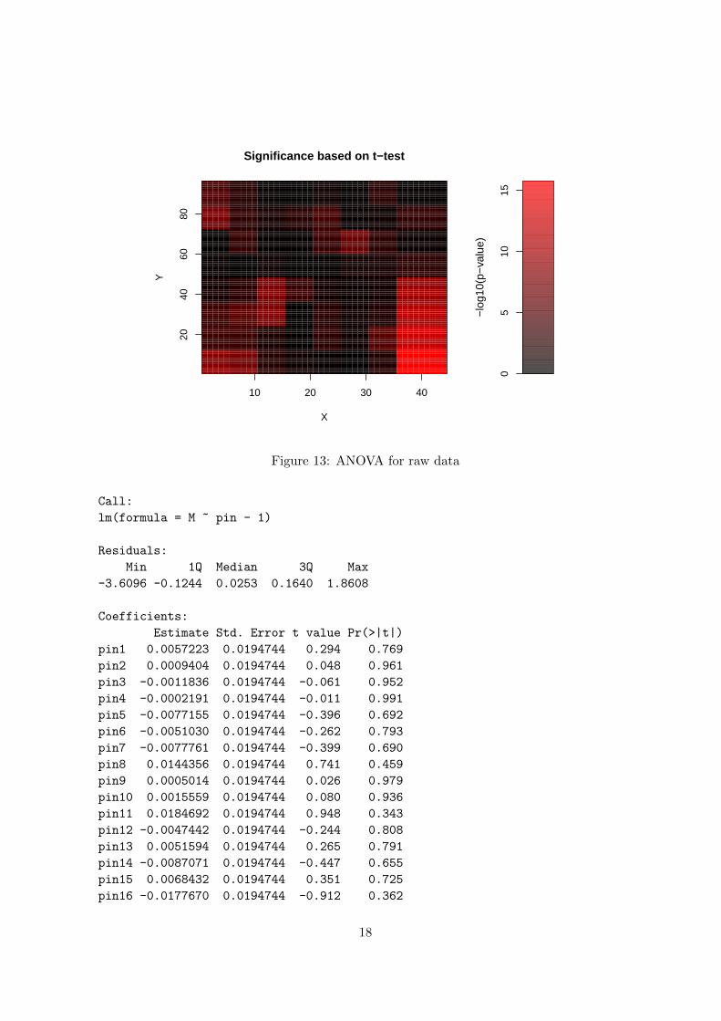
Similarly, the location-dependent bias can be examined by an ANOVA model implementedas anovaspatial. The array is divided into (xN x yN) rectangular blocks. The null hypothesistested is the equality of the means of M for the different blocks. The function anovaspatial
is a wrapper around functipn lm. The output is the summary of lm (which is suppressedin following examples). Additionally, anovaspatial allows for visualisation of the results(see figure 13 and 14.) The figures display the log10-transformed p-values as derived in theblock-wise t-tests. Note that the differences in scales.
> anovaspatial(sw,index=3,xN=8,yN=8,visu=TRUE)
> anovaspatial(sw.olin,index=3,xN=8,yN=8,visu=TRUE)
Additionally, simple one-factorial ANOVA models were implemented to test microarraydata for pin- and plate-dependent bias. Testing for pin bias by anovapin is similar to testingfor spatial bias by anovaspatial. The factors in anovapin are the pin indices. The nullhypothesis is the equality of the means of M for the different pins. In the same manner, itcan be tested if there is a significant variation of M due to the use of distinct microtiter platefor spotting. An ANOVA model for this task is implemented in function anovaplate.In thiscase, the null hypothesis is the equality of the means of M for the different plates.
> print(anovapin(sw.olin,index=3))
17
10 20 30 40
2040
6080
Significance based on t−test
X
Y
05
1015
−lo
g10(
p−va
lue)
Figure 13: ANOVA for raw data
Call:
lm(formula = M ~ pin - 1)
Residuals:
Min 1Q Median 3Q Max
-3.6096 -0.1244 0.0253 0.1640 1.8608
Coefficients:
Estimate Std. Error t value Pr(>|t|)
pin1 0.0057223 0.0194744 0.294 0.769
pin2 0.0009404 0.0194744 0.048 0.961
pin3 -0.0011836 0.0194744 -0.061 0.952
pin4 -0.0002191 0.0194744 -0.011 0.991
pin5 -0.0077155 0.0194744 -0.396 0.692
pin6 -0.0051030 0.0194744 -0.262 0.793
pin7 -0.0077761 0.0194744 -0.399 0.690
pin8 0.0144356 0.0194744 0.741 0.459
pin9 0.0005014 0.0194744 0.026 0.979
pin10 0.0015559 0.0194744 0.080 0.936
pin11 0.0184692 0.0194744 0.948 0.343
pin12 -0.0047442 0.0194744 -0.244 0.808
pin13 0.0051594 0.0194744 0.265 0.791
pin14 -0.0087071 0.0194744 -0.447 0.655
pin15 0.0068432 0.0194744 0.351 0.725
pin16 -0.0177670 0.0194744 -0.912 0.362
18

10 20 30 40
2040
6080
Significance based on t−test
X
Y
0.0
0.2
0.4
0.6
0.8
1.0
1.2
−lo
g10(
p−va
lue)
Figure 14: ANOVA for normalised data
Residual standard error: 0.3164 on 4208 degrees of freedom
Multiple R-squared: 0.0007643, Adjusted R-squared: -0.003035
F-statistic: 0.2012 on 16 and 4208 DF, p-value: 0.9997
> print(anovaplate(sw.olin,index=3))
Call:
lm(formula = M ~ plate - 1)
Residuals:
Min 1Q Median 3Q Max
-3.5987 -0.1278 0.0261 0.1658 1.8466
Coefficients:
Estimate Std. Error t value Pr(>|t|)
plate1 -0.0226044 0.0161246 -1.402 0.161
plate2 0.0287166 0.0161246 1.781 0.075 .
plate3 -0.0057500 0.0161246 -0.357 0.721
plate4 0.0018882 0.0161246 0.117 0.907
plate5 -0.0125836 0.0161246 -0.780 0.435
plate6 -0.0015375 0.0161246 -0.095 0.924
plate7 0.0003773 0.0161246 0.023 0.981
plate8 -0.0128983 0.0161246 -0.800 0.424
plate9 0.0157338 0.0161246 0.976 0.329
19

plate10 -0.0134014 0.0161246 -0.831 0.406
plate11 0.0223422 0.0161246 1.386 0.166
---
Signif. codes: 0 aAY***aAZ 0.001 aAY**aAZ 0.01 aAY*aAZ 0.05 aAY.aAZ 0.1 aAY aAZ 1
Residual standard error: 0.316 on 4213 degrees of freedom
Multiple R-squared: 0.002391, Adjusted R-squared: -0.0002133
F-statistic: 0.9181 on 11 and 4213 DF, p-value: 0.5216
ANOVA methods assume normality of the analysed data. This, however, may not bethe general case for microarray data. To relax this restriction, permutation tests can beapplied. Permutation (or randomization) tests have the advantage that a particular datadistribution is not assumed. They rely solely on the observed data examples and can beapplied with a variety of test statistics. A major restriction, however, is that permutationtests are computationally very intensive. Generally, such tests are not used in interactivemode but are performed in batch-mode.
Four permutation tests procedures were implemented in the OLIN package. The func-tions fdr.int and p.int assess intensity-dependent bias. The functions fdr.spatial andp.spatial assess location-dependent bias. The basic procedure is similar for all four func-tions. First, a (intensity or location) neighbourhood of spots is defined similarly to theprocedure we used for the correlation analysis . Next, a test statistic is constructed by cal-culating the median or mean of M the spot’s neighbourhood of chosen size. An empiricaldistribution of the test statistic M is then produced based on random permutations of thedata. Comparing M of the original data with the empirical distribution, the significance ofobserving M is derived. (Note that a rather low number of random permutations was chosento avoid time-consuming calculations here. Generally, however, a larger number should bechosen.)
The functions fdr.int, p.int, fdr.spatial and p.spatial perform two one-sided ran-dom permutation tests. The result can be visualised by the plotting functions sigint.plot
and sigxy.plot. The significance of a spot neighbourhood with large positive deviations ofM is displayed in red along the A-scale or across the spatial dimensions of the array. Cor-respondingly, the significance of spot neighbourhood with large negative deviations of M aredisplayed in green.
> FDR <- fdr.int(maA(sw)[,3],maM(sw)[,3],delta=50,N=10,av="median")
> sigint.plot(maA(sw)[,3],maM(sw)[,3],FDR$FDRp,FDR$FDRn,c(-5,-5))
> data(sw.olin)
> FDR <- fdr.int(maA(sw.olin)[,3],maM(sw.olin)[,3],delta=50,N=10,av="median")
> sigint.plot(maA(sw.olin)[,3],maM(sw.olin)[,3],FDR$FDRp,FDR$FDRn,c(-5,-5))
For slide 3, an significant intensity-dependent bias towards channel 2 (Cy3) was detectedfor low spot intensities, whereas high-intensity spots are biased towards channel 2 (figure 15).After OLIN normalisation, no significant intensity-dependent bias is apparent (figure 16). Asimilar result can be found for the removal of location-dependent bias by OLIN (figure 17 and18).
20

●
●
●
●●
●
● ●●
●
●● ●
●
●●
●
●
●● ●
● ●
●
●
●●
●
●●
●
●●
●
●
●●
●
●
●● ●●
●
●● ●●●●
● ●● ●
●
●
●
● ●●●
●●●●
●● ●
●●
●●
●● ●
● ●
●
●●
●●●
●●
●●●
●●
●●
●● ●●● ●●●
●
● ●●●
● ●●●
●
●● ●
●●
●●
●
●●●●
●
●●●
●
●
●●● ●
●● ●
●●
● ●● ●● ●
●
●●●
●
●●
●●
●●
●
● ●●●● ●● ●
● ●
●●●
●●
●●
● ●
●●
●●●
●
●
●●
●●
●●
●
●
●●● ●
● ●●
●●●
●
●
●●●
●
● ●● ●●
●● ●● ●●
●
●●●
●
●
●
●●
●●
●●
● ●
●●
●●
●
●●
●●
●●●
●●
●
●
●
●
●●●
●
●●●
●
●
●
●
●
●●
● ●●●●
●●
●●
●●●
● ●● ●● ●● ●●
●
●● ●●
●●
●●●
●
●●●
●●●
● ●●●●● ●
● ●●
●●
● ●● ●●
●● ●
●●●●●●
●
● ●●
●
●
●●
●
●
●
● ● ●
●
●
● ●●● ●
●
●● ●
●●
●●●●
●●●
● ●
●●● ●● ●
● ●●
●●
●●●●
●● ●
● ●●●
●
●
● ●
●●● ●
●● ● ●●● ●●●●● ●●
● ● ●●
●
● ●●
●
●●
● ●●
●● ●
● ●●
●
●●
●
●
● ●● ●● ●●
●
●●● ●●● ● ●
●● ●
●
●●
●
●● ●●
● ●●● ●
●
● ●
●
●●● ●● ● ●
●●
●● ●
●●●
●
●
●●●●
●●
●● ●● ● ●
●●●
●●
●●●
● ●
● ●●●●
●●
●
●
●●
●●●●●
●●
●
●
●
●
●●
●● ●
●●
●
●
●●
●●●
●● ● ●●
●●●
●●●● ●● ● ●
●
●●
●
●
●● ●● ●●
●● ●
●●● ●●●
●
●
●●
●
●●●
●● ●●
●●●
●
● ●●
●
●
●● ●
●●● ●●
●
●
●● ●●●
●●
● ●●●
●●●
●
●
●●
●
●● ●
●
● ●●
●●●●●●
●●
●●
●
●●● ●●
●●●●●
●
●
●
●
●●
●
●
●●
●●
●●●
●●
●
●● ●● ● ●
●●
●●● ●
●●
●
●
●●
●
●
●●
●●
●
●●● ●● ●●●
●●
●
●●●
●
●
● ●
●
●
●
●
●● ●● ●
●●●●
● ●●
●
●
●
●
●●
●
●
●
●
●● ●●
●●●● ●
●●●
● ●●
●
●●
●
●●●● ●
●
●●
●
●●● ●● ● ●
●
● ●
●●●
●●●
●●
●
●●
●●
●
●
●
●
●
●●
●●●
●●
●
●
●
●●
●
●
● ●●
●
● ●●● ●●
● ●●
●
●●●
● ●● ●● ●●
●
●
●
●
● ●● ●●
●
●●
●
●
●
●
●
●
●
●●
●● ●
●●
●
●
●
● ●●
●
●
●
●
●
●
●
●
●●
●
●●
●
●●
●
●●
●●
●
●●
●
●
●●●
●●
● ●
● ● ●●
●● ●
● ●
●●●
●
●
●
●
●●
●●
●●
●●
● ● ●● ● ●●●●●
●
●
●
● ●● ●
●●
●
●● ●●
●
●
●
●●
●
●
●
●
●●●
● ● ●
●
●
●
●● ● ●
●
●●
●
●
●
●
●●●
●●
●●
● ● ●●●
●● ●●
●●●
●●● ●●● ●
●
●
●●● ●● ●
●
●●● ●
● ●●●
●●●●●
●●
●● ●
●
●●
●● ● ●●
●
●●
●●●
●
●
●●●
●●
●●●●
●●
●
●
●●●
●●
●
●
●
●● ●
●
●●●
●●●
●
●●
●
● ●
●
●●
●
●
●
●●●
●●
● ● ●
●●● ● ● ● ● ●
●
●
●●
●●
●●●
●●● ●●●
● ●
● ●
●●
●●
●
●●
●
●
●
●
●
●
●
●●
●●●
●●
●
●
●
●
●●
●
●●●
●●
●●
●●
●
● ●
●●
● ●●
●●
●●
●●
●●
●
●
●
●●
●
● ●●
●●
●●
●
● ●●●● ●
● ●●●
●
●
●
●
●
●●
●●
●●
●
●
●● ●● ●●
●
●●●
●●
● ● ●●
●
●●
●
●
●
●●
●
●
●
●
●● ● ●
●
●● ●●
●●
●
●●
●
●●
●
●
●
●
●
●
● ●
●
●●●
●
●
●●
●● ● ●
●●
●
●
●
●
●
●
●
●
●●● ●●●
●
●●
●
●●
●●●
●●
●
●
● ●
●
●
●●●●●●
●
●
●●●
●
●●●●
●
●●●●
●
●●
● ●
●●
●●
●●●
●●●
●
●●
● ●●●●
●●●●
●●
●
● ●
●
●●
●
●●● ●●● ●●●
●
●
●●●●
●●
●
●
●
●
●● ●
●
●
●●●
●●●● ●
●
●
●
●●●●●
●
●
●● ●
●
● ●●
●●●● ●
●
●
●
● ●●●
●●
●●●●
●
●●
●
●
●
●●●
●●
●
●●●
●
● ●● ●
●
●
●
● ●●
●
●
●
●●
●
●
●
●● ●
●●●
●●●
●
●● ●
●●●
●
●
●
●● ●
●
●● ●●
●● ●●
●
●
●
●●
●
● ●●●
●
●●
● ●●●
●●
●●
●
●●
●●●
●
● ●
●
●●
●● ●●●
●
● ●●
●
●
●
●●
●●●
●
●
●●●
●
●
●●
● ●●●
●●
●●
●●
●
●● ●
●
●
●
●●
●●
●●
●
●
●●●
●●
●
●● ●● ●●
●
●●
●
●
●
●
●
●● ●
●●●
●
●
●
●●●
● ●
●●
●●
●
●●
●
●
● ●
●
●
●●
●
●●
●
●●●●
●● ●
●
●●
●
●
●
●●●
●●
● ●●
●
●
●
●●
●● ●
●●●
●
●●
●● ●
●
●
●
●
● ●
●
●●●
●●
●
●
●● ●
●●
● ● ●●●●●● ●
●
●●●
●●
●
●●●
●●
●●●
●● ●
●●●
●
●●
●●
●●
●
●●●
●●●
●
●●
●●●
●●
● ●●
●●
●
● ●●
●● ●
●●●
●
●● ●●
●
●
●
●●
●
●
●● ●● ●●
●●
●●●
●●●●
●●●●● ●●●● ●
●
●
●●●
●
●
●●
●
●●
●●
●●●●
●●●
●●
●
●●●
● ●● ●●
●●
●●●
●●●
●●●
●●
●●●
●●●
● ●●●
●●
●●
●●●● ●●●●
●
●●
●●
●●●
●
●
●
● ● ●●●
●● ● ●
●
● ●
●
●●
●● ●● ●●
●
●
●
●
●●●
●
●
●
● ●●
●
● ●●
●
●●
●
●●
●
●
●
●●●
●
●
●●
●●
●●
● ●●
● ●● ●
●
●●
●●
●●
●
●●
●● ●● ●
●● ●
● ● ●
●
●●
●●●
●●
●●
●●
●● ●● ●●●
●
●● ●
●
●●
●
●●●
●
●
●
●
●●
●●●
●
● ●●
●
●
●●
●●
● ●● ●
●●
●
●●
●●●●●
●●●
●
●
● ●
●●
●●
● ●
●
●●
● ●● ●
●
●●
●●
●●
●●
●●
●
●● ●
●●
●●
●● ●●●
●
● ●●
● ●
●●
●●
● ●
●
●
●●● ●
●●
●●●
●●
●●●●
●●
●
●● ●●
●
●
●
●
●
●● ●
●
●
●
●
●
●
●
● ●
●
●●
●
●●
●
●●●
● ●●
●
●
●
●
● ●●
●●●
●
●●●
●●
●●
● ● ●●● ●
●
●
●
●
●● ●
●●
●
●
●
●● ●
●● ● ●● ●
●●●
●
●
● ●
●●
●
●
●●
●●
●
●●
●●
●●
●
●●
●
●
● ●
●
●●
●●
●
●
●
●
● ●●
●●
●●
●
●●●
●
●●●●
●●
●●
●
●●●
●●
●
● ●
●
●● ●
●●
●
●
●●
●
●
●
●
●
●● ●● ●
●●
●●
●
●
●●
●●
●
●●
●
●
●
●
●
● ●
●
●
●●●●
●●●
●●●
●●
●
●
● ●●●●
●
● ●
●●
●
●
●●
●●
●
●
●●
●●●
●●
●●●
●
●
●
●
●●
●
●●
●
●
●
●
● ●●
●
●
●
●●●
●●
●
●
●●●
● ●
●
●●
●
●●
●●●
●●
●
●
●●
●●
●
●
●
●
●●
●
●●
●● ●●● ●● ●●
●●
●
●
●●
●●
●
● ● ●●
●
●●
●
●
●
●
●●
●
●● ●●
●
●
●
●
●
●
●
●●
●●●
●●● ●
●●●
●
● ● ●●●
●
●
●●
● ●
●●●
●●
●
●●
●●
●
● ●●
●●●●
●●
●●●
●
●●●
●●
● ●●
●
●
●
●●●
●
●
●
●●
●
●
●
●
● ●
●
● ●●
●●● ●● ●
●
●
● ●
●
●●
●
●
●
●
●
● ●●●●
●
●
●●
●
●
●●
● ●●●
●● ●
●●
●●
●
●
● ● ●● ●
●●
●●
●
●●●
●● ●●● ●
●
●●
●●
●
● ●●●
● ●●
●●
●
●●
●
●
●
●
●●●
●● ●
●
●●
●●●
● ●●
●●
●●
●
●● ●●
●
●●● ●
●●
● ●●
●● ●●
●●
● ●●
●
●●
●●
●
●
●
●
●
● ●
● ●●●
●
● ●
●
●
● ● ●●
●●
●●
●●●
●● ●●
●●
●
●●
● ● ● ●●●● ● ●●●●● ●
●● ●●●
●●●
●
●
●●●
●
●
●
● ● ●●
●●●●
●
●● ●
●●●
●●● ●
●●
●●
●●
●●
● ●●●
●●●
●●●●
●
● ●●●
● ●●● ●
●
●●
●●
●
● ●●●
●●
●
●
●●●
●●●
●●●
●
●●
●
●
●
●●
● ●
●
●
●
● ●●●
●●
●●●●
●● ●●
●
● ●
●
●●
●
●●
●
●●
●
●
●●
●
● ●
●●● ●
● ●
●
●●
●●●
●●
●●
●
●● ● ●
● ● ●
●●●
●●●
●●
● ●
●●●●
●●●
●
●
●●
●●● ●
●●
● ●
●●
●●● ●
●●
●
●●
●●
●
●●●●
● ● ●
●
●
● ●●
●●
●●
●●
●
●● ●●
●
● ●●
●
●
●
●●
●●
●
●●
●
●
● ●
●●
● ●
●
●
●
●●
●
●
●
●●●
●
●
●
●●
●●
●●●
●●
●
●
●●● ●
●●
●
●
●
●
●
●
●
● ●
●
●
●
●
●●
●●
●
●● ● ●●
●● ● ●
●
●●● ●●
●
●●
●●
●● ●
●
●
●●
●●
● ●●●
●●●
●●
●
●
●
●
● ●
●
●● ●
●
●●
●●●
● ●
●
●● ●●
●● ●
●
●
●
●
●
●
●
●
● ●
●● ●
●
●
●
●●
● ●●
●●
●
●●
●
●●
● ●●
●●
●
●
●
●●●
●
●●●
● ●●
●
●
●●
●●● ●
●●●●
●
●
●●●
●
●●●
●●
●
●
●●●●
●●●
●
●
●●●●
● ● ●●●
●
● ●
●● ●
●
●
●
●
●
●●
●
●
●
●●
●●
●
●●
●
●
●
● ●●
●
●●
● ●● ●●
●
●●●● ●● ●
●●
● ●●●
●
●
●●
●●
●●
●
●●●
●
●
● ●●●●
●
●
●
●●●
●
●
●
● ●
●
●● ●●
●●
●●
●●●
●
●●
●
●
●
●●
●
●
●
●
●
●
●●
●
●●
●●
●●●
●
●
●
●●
●
●
●
●●
●●
●●●
●●●●● ●
●
●
● ●
●
●●●
●●
●●
●
●
● ●
● ●
● ●
●● ●
●
● ●●
●
●●
●
●● ●● ●●
●
●
●
●
●
●
●
●● ●
●●
●●
●●
●
● ●●
●
●●
●
●
●
● ●● ●● ●
●
●
● ●
●
●
●●
●
●●
●
● ● ●●
● ●
●
●●
●●
●
●
●●
●
●
● ●
●
●
●●●
●●
●● ●
●● ●●● ●
●
●●
●
●
●●
●●
●●●
●● ●●
●●● ●● ●●
● ●
●
●●●
●●●●●
●●●
●
●
● ●●
●● ●
●
●● ●
●
●●
● ●●●●●
●●●● ● ●
●●
●● ●●●
●●
●● ●●●
●
● ●
●
●●
●
● ●●●
●
● ●
●●
●
●
●●
●●
●●
●
●
●●
●
● ●
●
●
●●
● ●● ●
●
● ●
●
●●
●●● ●●
●
● ●●●●● ●
●
●●
● ●●●
●●● ●
●● ●●
●
●
●●●
●●●●● ●
●
●
●
●
●
●●●
●
●
●
● ●●
●
●
●●●
●
●●
●●●●
●
●
●
●
●
●
●
●●●
●●
●
●●
●
●
●●
●
●●
●●● ●●
●●
●●
●
●●
●
●
●
●
●
●
●●
●
●
●
●●
●●
●
●●
●●
●●
● ●●●●
●●● ●
●●●●● ●
●●
● ●
●●
●
●●
●
●
●●
●
●●
●●
●
●● ●
●
●
●●●
●
●
●
●●
●●●
●
● ●●
●
●● ●
●
●
●●
●●
● ● ●● ●●
●●
●●●
●●
●
● ●●●
●●
●
●●
●
●
●●●
●●
●
●
●●
● ●● ● ●●● ●● ●
●
●
●●
●
●●
●
●
●
●●●● ●
●
●
●●●
●●
●
●
● ● ●●
●
●
●●
●
●●
●●●● ●●
●●
●●
● ●
●
●
●●
●●
●●
●
●
●●
●●●●
●●
●●
●● ●
●
●
● ●●●●
●
● ● ●● ●●●
● ●●● ●●
● ●
● ●●●
●
●●●●
●
●●
●
●●
●●
●
● ●●●
● ●●● ●
●
●●
●
● ● ● ●●●
●
●
●● ● ●
●
●
●● ●
●●
●
●●
●
●
●●●●
●
● ●●● ●●●●● ●
● ●●
●
●●
●
●
●●
●●
● ●●●
● ●
●
●
●
●●
●
●
●
● ●●●
●●●
●●●
●
●
●
●●
●
●●●●●
●
● ●●
●
●
●
● ●●
●●
●●●
●●
●
●●
●●
●●
●●
●
●●
●
●
●
●
●● ●
●●●
●●
●
● ●●
●●
●
●● ●
●
●
●
● ●●
●
●●
●
●●●
●●● ●
●
●
●●●
●●●
●
●
●
●
●
●
●
●
●
● ●●●
●
●
●●
●
●●
●●●
●
●
●● ●●●●●
●
●
●
●●
● ●
●●●
●●●
●●
●●
●●●
●
●
●
● ●
●
●● ●●●
●●
●
●●
●●
●●
●
●
●
●●
●
●
●●
● ●● ●
●
●
●●
●
●●●
●
●●
●●
● ● ●●
●●
●
●
●
●●
●
●
●●
●
● ●●
●
●●
●
●
●
●●
● ●●●
●
●●
●●●●
●
●●●
●
●
●
●
●
●
●
●● ●●●
●●●
● ●
●
●
●
●
●●
●
●
● ●●
●● ●
●
●● ●
●
●
●
●●
●
●
●●
●●
● ●
9 10 11 12 13 14 15 16
−4
−3
−2
−1
01
2
MA plot
A
M
●
●
●
●
●
●
●●
●
●
●● ●
●
●
●
●
●
● ●
●●
● ●
●
●
●
●●
●
●
●
●
●
●
●
●
●
●●
●
●
●
●
●
●
●●
●●●
●
●
●
●
●●
●
●
●
●
●
●●
●
●●
●● ●●
●
●
●
●
●
●
●
●
●
●
●
●
●●
●●
●●
●●
●
●●
●
● ●
●
●
●●●
●●
●
●
● ●
● ● ●
●●
●
●
●
●●
●●
●
●
●
●●
●●
●
● ●
●●● ●
● ●
●
●
●
●
●
●●●●
●
●
●●●
●● ●
● ●●
●
●●
●
● ●
●
●●●●
●●
●
●●
●●
●
●●●
●
●
●
●
●
●
●●
●● ●
●
●
● ●
●●
●
●●
●
●
●
●
●
●●
●
● ●
●●
●
●●
●
●●
●
●
●
●
●● ● ●● ●●●●
●
●
●
●
●
●
● ●
●
●
●
●
●●●
●
●
●
●●●
●●
●
●
●●
●
●
●
●●●
●
●
●●
●
●●
●● ●
●
●●
● ●●
●
●
●
●
●● ●
●
●
● ●●
●
●●●
●
●
●
●●● ●
● ●
●
●
●
● ●
●
●
●
●●
●
●
●
●●
●
●
● ●
●● ●
●
●
●
●●
●
●
● ●
●
●●
●
●●
●
●
●●
●● ●● ●
●
●
●
●
●●● ●
●
●
●
●
●
●●
● ●
●●
●●
●
●
●
●
●
●
● ●
●●
● ●●
●●●
●
●●
●
●
●
●
●●● ●
● ●●
●
●
●●
●
●●
●
● ● ●
●
●
●
●●
●
●● ●
●
●
●
●
●
● ●
●
●●
●●
●
●
●
●
●●●●
●
●
●●●
●●
●
●
●
●
●
●●
●
●
●
●
●
● ●
●
●
● ●●
●● ●
●
●
●●● ●
●●
●
●
●
●●
●
●●
●
●
●●
●
●
● ●● ●●
●
●
●
●
●●
●
● ●
● ●
●●
●
●
●
●
●●
●
●● ●
●●
●
●
●
●
●
●
●●
●●●
● ●
●
●
●
●
●
●
●●
●
●
●
●
●●
●
●
●
●●
●
●●
●
●
●●
●
●
●
●
●
●
●
● ●●
●
●●
●●
● ●
●
●●●
●
●
●
●
● ●
●
●
●
●
●
●
●
●
●
●
●
● ●●
●
●
● ●
●
●●● ●
●
●
●
●
●
●●
●
●●●
●
●
●●
●
●
●
●
●
● ●
●
●
●
●●
●
● ●
●
●●
● ●●
●●
●
●●
●●●
●
●
● ●
●
●
●●
●
●●
●
●
●
●
●
●
●
●●
●
●
●
●
●
●
●
●●●
● ●
●
●
●
●
●●
●
●
●
●
●
●
●
●
●
●
●●
●
●
●
●
●
●
●
● ●●
●●
●●
●
●
●
●
●●
●●
●
●
●
●●●
● ● ●●
●
●●
●
●● ●● ●
●●
●
●
●●
●
●
●
● ●
●
●
● ●●
● ●
● ●
●
●
●●
●
●
●●
● ●
●●
●
●
●
●
●
●
●
●
●
●●
●
●●●
●●
● ●●
●
●
●
●●
●
●
●
●
●
●
●
●
●
●
●
●●● ●
● ● ●
●
● ●
●
●
●
●
●
●
●
●●
●●
●
●
●
●● ●
●
●
●● ●
●
●● ●
●
●
●●
●●
●●
● ●
●
●
●●●
●
● ●●
●●
●
● ●
●
●
●
●
●
●
●
●
●
●
●
●
●
●
●
● ● ●
●
●
●●
●●
●
●
●
● ●
●
●
●
●
●
●
●
●
●● ●
● ●
●
●
●
●
●
●
●
● ●
●
●
●
●●
●● ●
●
●
●
●
●
●
●●
● ●
●
●
●
●
●
●
●
●
●●
●
●
●●
●
●
●
●
●
●●
● ●
●
●
●
●
●
●●
●
●●
●
●
● ●
●
●
●● ●
●
●
●
● ●
●
●
●
●●●
●
●
●
●●
●
●●●●
●●●●
●
●
●
●
●
●
● ● ●
●●
●
●
●●●●
●
●
●● ●
● ●●
●●
●
●●
●●● ●
●
●
●
●● ● ●
●
●
●
●●
●●
●●
●
●
●
●●
●●
●●
●
●
●
●
●
●
●
●●
●
●
●●● ●
●
●●
●
●
●
●
●
●
●
●
● ●
●
●
●
●
●
●
●●
●
●
●
●
● ●●●
●
●
●●
●
●
●
●
●●●
●
●●
●
●
●
●
●
●
●●
●
●●
●
●
●
●
●
●
●
●●
●
●
●●
●
●
●
●
●
●
●
●●●
●●
●
●
●
●
●
●● ●
●
●●
●
●●●
●●
●
●
●
●
●
●
●
●
●
●● ●
●
●
●
●
●● ●
●
●
●
●●
● ●
●
●
●
●
● ● ●
●●
●
●● ●
●
●● ●● ●
●
●
●
●
●
●● ●● ●●
●●
●
●
●●
●
●●● ● ● ●●●●●●
●
● ●
●
●
●
●●●●●
●●
●●●
●
●
●
●●
●
●●●
●
●
●
●
●●
●
●
●
●●
●
●
●●
● ●
●●
●●●
●●●
●
●●
●
●
●
●
●
●
●
●
●
●
●
●
●
●
●
●●
●
●
●
●
●●
●
●
●
●
● ●●
●
●●
●
●
●●
●
●
●
●
●●
●
●●●●
●
●
●
●●
●
●
●
●
●
●●● ●
●
●
●
●
●
●
●
●
●●●
●
●●
●
●
●
●
●
●●●
●
●
●
●
●
● ●●
●●
●
●● ●
●●
●
●
● ●
●●
●
●
●
● ●●
●●
●
●
●
●
●
●●
● ●
●
●
●
●
●
●
●●
●
●
●
●
●
●
●
●
●
●
●
●
●
●
●
●
●●● ●
●
● ●●
●
●
●
● ●
●●
●
●
●
●
●
●
●
●
●
●●
●●
●
●●
●
● ●
●
●
●●●
●●
●●
●
●
●
●
●
● ●●
●
●
●
●●
●●
●●
●
●●
● ●
●
●
●
●
●
●●
●
● ●
●●
●
●●●
●
●
●
●
●
●
●
●
●
●
●
●
●
●
●
●
●
● ●
● ●
●
●●
●
●●
● ●
●
●
●
●
●
●
●
●
● ●
●
●
●
●
●
●
●
●
●●
●●
●
●
●
●
●
●●
●
●
● ●
●
●
●● ●
●●
●
●
●
●● ●
● ●●
●
●●● ●
●●
●●
●
●
● ●
●
●
●
●
● ●
●
●●●
●●
●
●
● ●
●
●
●●
●
●
●●
●
●
●
●
●
●
●
●
●
●
●
●
●
●● ● ●
●
●
●
●
● ●●●
●
●● ●
●●
●●
●
●
●
●
●
●
●
●
●●
●
●
●
●
●
●●
●
●
●
●
●
●●●
●
●
●
●
●
●
●
●
●
●●
●●●●
●●
●
●●
●
●
●
●●●
●
●
●●
●
●●●● ●●●●
●●
●●●
●
●
●
●● ●
●
●
●
●
●
●
●
●●●
●
●
●
●
● ●
●
●
●
●
●
●
●●●
●
● ●
●
●
●
●
●
●
●
●
●
●
●
●
●
●●
●
●●
●
●●
●
● ● ●
●
●
● ●●
●
●
●●
●
●
●●
● ●
●
●●
●
●
●
●
●
●
●
● ●●● ●● ●
●●
●
● ●
●
●
●●●
●
●●●
●
●
● ●
●● ●
●
●
●
●
●
●●
●
●●
●
●
●●
●
●
●●
●
●
●●
●●
●
●●
●
●
●
●
●
●●
●
●
●
●
●
●
●●
●
●●
●
●●
● ●
●●
●●
●
●
● ●
●
●
●
● ●
●
●●
●
●
●
●●
●
●
●
●
● ●
●
● ●
●
●●
●●
●●
●
●
●
●
●
●
●
●
●●
●●
● ●●
●●
● ●
● ●●
●
●
●●
●
●
●
●
●● ●
●●
●
●
●
●●●●
●●
● ●●
●
●
●
●
●
●●
●
●● ●
●
●
●
●●
●●●
●
●
●
●
●
●
●
●●
●● ●● ● ●● ●
●
●
●
● ●
●
● ●
●
●
● ●● ●
●
●
●
● ●●
●
●
●
●
●
●●
●
●
●●●
●
● ●●
● ●
●
●
● ●
●●
●
●
●
●
●
●
●
●
●
●●●
●●
●
●●
● ● ●
●
● ●
●
● ●
●
● ●●
●
●
●
●
●
●●
●●
●●
●●●
●
●● ●●
●
●
●●●●● ●
●●
●● ●
●
●
●●●
●
●●●
●
●
●●●●
●
●
●
●
●
●
●
●●● ● ●● ●●
●
●
●
●
●
●
●
●●
●
●
●
●● ●
●
●
● ●
●
●●
●●
●
●●
●
●
●
●
●●
●●
●
●
● ●●●
●
●
●
● ●
●
● ●● ●
●
●●
●●●
●
● ● ●●
●●
●
●
●
●
●●
●
●● ●● ●●●●●
●
●●
●●
●●●
●
● ●●
●
●
● ●
●●●● ●● ●● ●● ●● ●
●
●
●
●●
●● ● ●●
●
●
● ●
●
●
●●
●
●
●
●●
●
●
●
●
●
●●
●
●
●
● ●
●●●
●
●
●
●
● ●
●
●
●●●
●
●
●
●
● ●
●●
● ●
●
● ●
●
●
●
●
●
●
●
●
●
●
●
●●
●●
●●●
●
●
●●●
●
●
●
●
●
●
●
●●
●
●
●
●
●●
●
●
●
●
●●●●
●
●
●
●●
●
●●
●●
●●
● ●
●●●
●
●● ●● ●
●
● ●●
●
●
●
● ●
●
●● ●
●
●
●
●●●
●●
●●
●
●●
●
●
●
●● ●●
●
●
●
●●
●●
●
●
●●
●●
●
●●
●●●
●●
●
●●
●
●●
●
●●●
●
●
●●
●
● ●
●
●
●● ●
●
●●
●●●
●●●
●
●
●●
●●
●
●
●●
●●
●
●
●
●
●
●
●
●
●
●
●
●
●
●
●
●●
●
●
● ●● ●
●
●●● ●●●● ●
●
●
●● ●●●●●●●● ● ●● ● ●● ●●● ● ●
●
● ● ●
●
●
●
●●
● ● ●
●●
●
●
●●
●● ●● ● ● ●
●●
●
●● ●
●
●
●
●●
●
●
●
●●
●●●● ●●
●●
●
●
●
●● ● ●● ●
●
●● ●
●
●
●
●●
●
●
●
●
● ● ●● ●● ●● ●●
●
● ● ●●
●
●
●
●
●
●
●
●●● ● ●● ●●●●●● ●● ●●● ●●●● ●●●●●● ●●● ● ●●
●
●
●
● ●●
●
● ●● ● ●●● ●● ●●● ●
●
● ●● ●● ●●●● ●●
●● ●
●
● ●●●● ●
●
●● ●
●
● ● ●● ●●●● ●● ●● ●●● ● ● ●●
●
● ●●● ●●●
●
●●
●●●●●●● ●● ●●●● ●
●
● ●● ●● ● ●●● ● ●● ●●● ●●●
●●●● ● ● ●● ●
●
●
●
●
●
●
●
●
●●●●
●
●●
●
●
●
●
●
●
●
●
●
●
●
●
●● ● ●
●
●
●
●
●
●
●
●
●
●
●
● ●●
●
●
●
●
●
●
●●● ●
●
●●
●
●
●
●
●
●●●
●
●
●
●
●
●
●
●
●●
●
●
●
●
●●
●
●
●
●
●
●
●
●
●
●
●
●
●●
●
●
●
●
●
●●
●
●
● ●● ●●●●●●●
●
●●●
●
●●
●●
● ● ●● ●
●
●
●● ●● ●●
●
●
●●
●
● ●●
●
●
●
● ●● ● ●● ●
●
●
●
●●●
●
●
●
●
●●
●
●●
●
●
●●
● ● ●
●
●
●
●
●
●●
●
●
●
● ●●
●
● ●
●
●●
●● ●
●
●●●● ●
●
● ●
●
●●● ●● ●●●●●● ●
●
●●●
●
●
●
●
● ●
●
●
●
●
●
●
●
●●
●
● ● ●●
●
●● ●● ●● ● ●
●
●● ●● ●● ●● ●● ●● ●●
●
●●
●
●●● ●●
●
●
●
●
●
●
●●
● ●
●
●
●
●● ●
●
●●
●
●
●
●
●●●● ●
●
●●●
● ●
● ●●
●
● ●
●
●●
● ●
● ●●●
●
●●
●
●
●
●
●
●●
●
●
●
● ●
●●
●
●
●
●●●
● ●
●
●●
●● ●● ●
●●
● ●●●
● ●
●
● ●● ●●
●
●
●
●
● ●
●
●●
●
● ●● ●●
●
●
●
●●
●
●●
●
●
●● ●● ●● ●● ●
●
● ●
●
●
● ●
●●
●
●●
●
●
●
●
●●
●●
●●●
●
● ●●
●
●
●● ●●●●
●
●●
●
●● ●
●
● ● ●● ●● ●●●●●
●●
●● ●●
●
●●●
●●●● ●● ●●
●● ●●●●
●●
●●●●
●
●●●● ●● ● ● ● ●●●●●
●
●●
●●
●
●
●
●●●
●
●●
●●
●
●●
●
●
●
●
●
●
●●
●
●
●●
●
●●
●●
●●
●
●
●
●
●●
●
●●●●
●
●
●
● ● ●
●
●●
● ●
●
●
●
●
● ●
●
●●
● ●
●
●● ●
●
●
●
●●
●
●
●● ●
●
●●
●● ●
●
●●●● ●●
●
●● ●
●
● ●●●
●
●●●
●●
●
●
●
●●● ●●●
●
● ●●●
●
●●
●●
●● ●● ●
●
●●●●
●
●●
●
●
●●●
●
●
●
●●
●
●
●
●
● ●
●
●
●●●
●●
●●
●
● ●
●
●●
● ●
●
●
●● ● ●●● ●
●
●
●
●
● ● ●●● ● ●●●●
●
● ● ●●●
● ●
●
●
●
●
●● ●● ●●
●
●
●
●●
●● ●● ●●●
●
●●
●●
●
●
●
● ●●●● ●●●
●●
●
●●● ● ●● ●
●
● ●
●
● ●
●●●● ●
●
● ●● ●● ●●●
●●
●
●
●
●●●
●
●
●
● ●●●
● ●●
●
●
●● ●●
●
●
●●●
●
●
●
●
●
●
●●
●●
●
● ●●●● ●
●
●
●
●●
●
●
●
●
● ●●●
●
●
●●
●
●
●
●
●●
● ●●
●
●●
●
●●●
●
●
● ●●
●
●
●●
●
●●
●
●
●
● ●
●
●
●
●
●
●●
●●● ●● ●●
●
●
●●● ● ●●
●
●● ●●
●
●
●
●●
●●●
●●
●
●●
●
●
●
●
● ●
●●
●
●● ●● ●●●
●
●
●
●
●
●
●
●
●●
●
●●
●
●
● ●●●●●
●●
● ●●
●
●
●
●●
●●
●
●●
●
●
●
● ●●●
●
●●
●●
●
●●● ●●● ●
●●
●
●
● ●●
●●
●
● ●● ●● ●●●●●● ● ● ● ●●
●
●● ●
●
●● ●●●
●●● ●●●●
●
●
●●
●
●●● ● ●
●
● ●●
●
● ●● ● ●● ●●
● ●
●● ● ●
●
●
● ●
●●
●
●● ●● ●●●●
● ●●●
●
● ●● ●● ● ●●● ● ●●
●
●
●
●
●
● ● ●●
●
● ●● ●●●● ●●●
●
● ●●●● ●● ●
●
●
●
● ●●● ●● ● ●●
●
● ●
●
●●
●●
● ● ●●
●
● ●
●
●
●●
●●
●
●● ● ●
●
●●●● ● ●● ●
●
●
●
●
●
● ● ●●
●● ● ● ●●
●
● ●●
●
●●
●
●
●
●
●● ●●●●● ●● ●●●●● ●●● ●●●
●
●●●●
● ●●● ●●● ●● ●● ●●
●
●
●
●● ●● ● ●●●● ●●●●
●
●● ●●● ● ●● ●●● ● ●
9 10 11 12 13 14 15 16
Significance
A
log1
0
●
●
●
●●
●
● ●● ●●● ●
●
●●
●
●
●
● ●●
● ●
●
●
●●
●
●
●
●
●
● ●●● ● ●●●● ●
●
● ● ●●●● ●●● ●● ●● ●
●
●● ● ●●● ● ●● ● ●●●●●● ●●● ●●● ●●●●● ●●● ● ●● ● ●● ● ● ●● ●●● ●●●● ● ●●● ● ●●● ●● ● ●●●● ● ● ●● ●●● ●● ● ●●● ● ●● ● ●●●● ●● ●● ●● ●●● ● ●● ● ● ●●● ●●● ● ●●● ●●●●● ●●
●●● ● ●●●
●
●● ●● ●● ● ●● ●● ●● ●● ●●● ●●● ●
●
●● ●●● ●● ●
●●
● ●● ●● ●●● ●●
●● ● ●● ●●●●
●●● ●● ●
●
●
●●
● ● ●●●● ●● ●●● ●●● ●● ●● ●●● ●●● ●● ●● ●●● ● ●● ●●● ●● ●● ●
●
●● ●● ●● ●● ●●●●
●
●
●
● ●● ●
● ●
●
●
● ● ●●
●
● ●●● ●
●
●● ●● ● ●●● ●
●
●● ● ● ●●● ●● ●● ●●● ● ●●●●● ●● ●●● ● ●● ●● ●● ●●● ● ●●● ●●●●● ●●● ● ●●
●
● ● ●
● ●●
● ●●● ●● ●
●
●
●
● ●● ●● ●● ●●
●
● ●● ●●● ● ● ●● ●● ●●● ●● ●●● ●●● ● ●● ●●●●● ●● ● ●●● ●● ● ●●●●● ●● ●● ● ●●● ●● ● ●● ●●●● ●●●
●
● ● ●●●● ● ●●●● ● ●●●●● ●●
●
●
●●
● ●
●
● ●
●
●
●
●
●● ●●
●
●
●
● ● ●●● ●●●● ●● ● ●● ●
●●
●● ●● ●● ● ● ●●●● ●●● ●● ●●
●
●● ●●● ●●● ●●
●
● ●●●
●
●● ● ● ●● ●● ●
●
●● ●●● ●●● ●● ● ●●
●●●
●● ●●● ● ●● ● ● ●●●● ●● ●
●
● ●● ●●● ●● ●●● ●● ●
●
●● ●●●●
●
● ●●●●● ●● ●●
●
● ● ● ● ●● ●● ● ●●● ● ●●●●● ●●●●● ● ●● ●● ●●● ● ●●● ●● ●●● ●●● ●● ●● ●● ●● ●●● ● ●● ●● ●●●●
●
● ● ●●
●
●●
●
●●● ●● ●
●
● ●
●
● ●●●● ●●● ●● ●
●
●
●●● ●● ● ●●● ● ●●●●●●
●●
●
● ●
● ● ●● ●●
●
● ●● ●● ●● ●●
●
● ● ●●● ●● ●● ●●● ●●● ●● ●● ●● ● ●● ●● ●●●●
●
● ● ●● ●●●●●
●
● ●●
●
●
●
●●● ● ●
●●● ●
● ● ●●
●
● ●
●
●●
●
●
●
●●●● ●
●
●
●●
● ● ●●● ● ●●● ●●●● ●
●
● ●●● ● ●● ●●●●
●
●
●
●●●● ●● ●●●●
● ●● ● ●● ●●●
●
●
●
● ● ● ●
●●
●●● ●● ● ●
●
● ●●● ●● ●●● ● ● ● ●● ●●● ● ●● ● ●● ●●●●
●
● ●● ●●● ● ●● ● ●● ● ●●● ●●● ● ●●● ● ●● ●●● ●● ● ●●●● ● ● ●●● ● ●●●● ●● ●● ● ●● ●●● ● ●● ●●
●●
●
●
●●
● ●●●● ●●●●● ●●
●
●● ●● ●●
●
●
● ●
● ● ●
●
● ●●
●
●
●●● ● ●● ●●●
●
●●●●
●
●
●
● ●●●
●
● ● ● ● ● ●● ●●
●
●
●●
●●● ●●●● ●● ●●
●
●● ●●●●●●● ● ● ●● ● ●● ● ● ●● ● ● ●
●
●●● ●●●
●
● ●●
●
● ●●●● ● ●● ●●● ●●●● ●●
●
● ●
●
● ● ●●●● ●●●
●● ●● ●● ●● ●● ●● ●● ●●●● ●●
●●
●● ●● ●● ●●● ● ●●● ● ●●●●●
●
●● ●●● ● ●●●
● ●
●● ●● ●● ●● ●●
●●
● ●● ●●●
●
● ● ● ●●
●
●
● ●●
●
●
●●
●●● ● ●
●●
●
●
● ● ●●● ●●● ●
●●● ● ●
●
●●●●●
●●
● ●● ●
●●●●●
●● ●●●● ●●●●● ● ●●●● ●●● ●●● ● ●●●● ●●● ●
●
●
● ●●●● ●●●●● ● ●● ●
●
●●● ●●● ●●● ●●● ●
●
●●● ●●● ●
● ●
●●
●●●● ●●●●●● ●●● ●●●●● ●
●
●● ●
●
● ●●● ●●● ●● ●● ● ●●● ●● ●●●●● ●●
●
●
●
●●●● ●
●
●●●● ● ●● ●
●
●● ● ● ●●● ● ●
●
● ● ● ●● ●● ●●●● ●● ●●●●● ●● ●●
● ●●● ● ●●● ●● ●●●
●● ●● ●
●
●● ●● ● ●●● ●● ●
●
● ● ●● ●● ●● ●
●
●● ●● ●●●● ● ●● ●● ●● ● ●●●●● ●●● ● ●●●● ●
●
●● ● ●● ●●●
●
● ●●
● ●
●● ●● ●●
●
● ● ●●
●
●●
●
●
●● ●●
●
●●●
●
●
●● ●● ●
●
●● ●● ●
●
● ●●●●
●
● ● ●
●
●● ●
●
●● ● ●●●●● ● ●
●
●●
●
●
●
●●● ●●
● ● ●
●
● ●●●● ● ●● ●●● ●● ●●
●
●
● ●●● ●
●
●
●● ●●
●
● ●● ●●
●
●● ●●●●●● ●
●
●
●●●● ●● ●●
●
●
●
●● ●● ●●●●●
●●● ● ● ●
●
● ●● ●●●
●●
●
● ●● ●● ● ●●● ●●
●
● ● ●● ●●●
●
●●● ●● ●●
●
●●● ●●
●
●● ● ●●● ●●●●● ●●●●● ●● ●●●● ●
●
●● ●●●
●
●
●●
●●
●●●●●
● ●●
●
●
● ● ●● ● ●● ●●●●
●
●●
● ● ●●● ●●● ●●●●●● ●● ●●●● ● ●● ● ●●●●●●● ● ● ●● ●●● ● ● ●● ●
● ●●
●● ●● ●● ●●
● ●
●●● ● ●
●
● ●● ●
● ●●● ●● ●
● ●●
● ●
●●●●
●
●●●●● ●
●
●● ● ●● ●
●
●●● ● ● ●●● ●
●●
●● ● ●● ●● ● ●●● ●● ●● ● ●●● ●
●
●● ●● ●●●● ●● ●●
●
● ●
●
●
●●
●
●
● ●
● ●●
●
●● ●●
●
● ●● ● ●● ●● ● ●●● ● ●●●●● ●●● ●
●
● ● ●
●
●● ● ●●● ●● ●● ● ●
●
● ●●● ●●● ●●●●
●
● ●●●● ●● ●●● ●
●
●
●
● ●●●● ●● ●● ●
●
●● ● ● ●●●● ●
●
● ●●●
●●
●●
●
●●
●
●
●
●
●
●
●●
●
●
●
● ●
●●
● ●
●
●● ● ●● ●
● ●●
● ● ●●
●
●●● ●
●
●●●
●
●
●
● ●●●
●
● ●●● ● ●●
●
● ●●
●●●
●
●● ●● ●
●● ● ●
●
● ●
●
● ●
●
●
●
● ●●● ●●● ●● ●●●●● ●●
●●
●
● ●● ●●●
●
●●
●
●
●
●● ●●●
●
●●●
●
● ●●●●
●
●
●
●● ● ●●●●
●
● ●
●
●
●
● ●●● ●● ●
●
●
● ●●●●
● ● ●
●
● ●● ● ●●● ●● ● ●● ●●● ●● ● ●● ●●
●
● ●●● ● ●
●
●
●
●●● ●●
●
●
●
● ●
●
●
●●
●
● ●●
●
●
●●
●
●
● ●●
●
●●
●●●●●
●●
●
●
●
●
●● ●● ●●
●●● ●● ●●
●
● ●● ●
●●
●
●
●
●● ● ●●
● ●● ●● ●
●
● ●●● ●● ●●●
●
● ●●● ●● ●● ●●● ●●● ●●
● ● ● ● ●●● ●●●●
●
●
● ●●● ●● ● ●
●
●
●
● ●●● ●●● ●●● ●●
●●●
● ● ●●●
●
●●● ● ● ●●●●●● ●●● ●
●
● ●●●●
● ●●●● ●
●
●●●
●●● ●● ● ●●●●●● ●
●
● ●● ●
●
●● ●
●
●
●●
●
●● ●● ●●
●
● ●●●●
●
●
●
●
●
● ●●● ●
●
●
●
●●● ● ●● ●●●
●
● ● ●●●●
●
●● ● ●● ●●
●
●
●●●
●
● ●● ●●
●●
● ●●
●
●
●● ●●●
●
●●● ●● ●●●● ● ●●● ●●● ●●
●
●●●●● ●●
●●●● ●●● ● ●
●
●
●
● ●●●
● ●●
●● ●
●
●
●
●
●
●
●●●●●● ● ●●
● ●
●
●
●● ●
● ●
● ●
● ● ● ●●● ● ● ●
●
●
●● ●●
●
●
●
● ●
●●
● ●●●● ● ●●●●
●
●●● ●●
●
●●●
●
●
●●●● ●
●
●
●
●
●
●●●
●
● ●● ●
●●
●
●●● ●
●
● ●
●
●
● ●●
●
●●
●
●
●●●● ●● ●
●
●
●●
●
●
●
● ●
●
●●●● ●● ●●●
●●
●● ●●●●●●
●
●●
●●● ●
●●
●
●
●
●
●
●
●
●
●
●●
●
●
●●
● ●
●
● ●
●
●●●
●
●●
●
●
●
●
●
●
●
●
●●●
● ●
●● ●
●
● ●
●
●
●
●●●
●
●
●● ●
●● ●
●
● ● ●
● ●
●
●
●●
●
●● ●
●●●●●●●
●
●
●
●●
●
●
●
●
●
● ●● ● ●●● ● ●● ●●●
●
●
●
●●●● ● ● ●●
●
● ● ●● ● ●
●
● ●●● ● ●●●● ●● ● ●●● ● ● ●● ●●●
●
● ● ●● ● ●●●●●● ●●
● ●●
●● ●●●●●
●● ●
● ● ●
●
●●● ●●●
●
●
●
●
●
● ●● ● ●● ●
●
●● ●
●●
●
●
● ●
●
●● ● ●
●
●●
●
●● ●
●
●●
●●● ●
●
●
●
●
●
●
●
●●● ●●●● ●
●
● ●●
● ●
●
●
● ●●●
●
●
●
●
●
● ●●
●
●
●
●
●
●
●
●
● ●●
●
●
●
●
●
●● ●
●
●●
● ●
●
●●
●
●●
●
● ●●●
● ●
● ● ●●● ●●● ●
●
●
●
●●●
●
● ●●●
●
●
●
●
●●
●●●
● ●
●
● ●●
●●
●
●
●
●●
●●●
●
●●●● ●● ●●
●
● ●●
●
●
●
● ●● ● ●
● ●
●
●
●
●
●
●
●
●● ●
● ●●
●
●
●
●
● ●
●
●
● ●●
●
●
●
●
●
●
●
●●
●
●
●
●
●
●
●●● ●
● ●
●● ●
●●
● ●●
●
●
●
● ●●●
●
●
●
●●
●
●
● ●●
●
●
● ●
●
● ●●
●
● ●
●●●
●
●●● ●●● ●
●
●● ● ●●● ●●
●
●●●●●● ● ●● ●●
●
●
●
●
●●● ●
●
●●●
●
● ●● ●
●
●● ●
●
●●
●
● ●
●
●
●
●
●
●
●
●
● ●●
●
●●● ●
●
●●
●
●
●
●
●
●
●
● ●● ●● ●●● ●
●
●
●●
●
●
●
●● ●●● ●●●
●
●
● ●
●
● ●
●●
●
●
●
●
●●
●
●●
●
●●
●
●
●
●
●
●
●
●
●
●●
●
●
●
●
● ● ●●
●
●
●
●●
●
●●
● ●●
●
●
●
●●
●●●●
●
●
●●●
●● ●● ●
●●
●●
●
●●
●●
●
●●● ●● ●● ●● ●● ●●●
●
● ●●●●●● ●●● ● ●●● ● ●●● ● ●●● ●●●●
●
●●●●●● ●● ●
● ● ●
●●●
● ●
●●
●
●
●
● ●●● ● ●●●
●
●
●● ●● ● ● ●●
●
● ●
●
●
●
●
●
●●●
●
●
●● ●
●
● ●●● ●●●●●
●
● ● ●● ●● ●
●
●
●
●
●
● ●● ●●● ●● ● ● ●●
●
●
●
● ●●●● ●
●
● ●●●●
●●
● ● ●●
●
●●
●
●
●
● ●● ●●●●●
●
●
●● ● ●●●
●
● ● ●●
●
● ●
●
●
●●●● ● ●
●
●
●
●
●
● ●●
●
●
●
●
● ●
●
●●
●●● ● ●
●● ●
●
●
●
●
●
●● ●●
●
●●
●●
●
● ●● ●
●
●
●●
●
●
●●
●●
●
●
●
●
● ●●
●
●
● ●
●
●●
●
●
●● ●
●
●
●●
●
●
●
●
●
●
●
●
●●
● ●
●
● ●●●
●●
●● ●
●
●●●
● ●●
●●
●
●
●● ● ●●
●
●● ●● ●●
●
●●●
●
●
●
●
●
●● ● ●● ●●● ●●● ●
●
●●● ●●●
●
●●● ●●●●● ●
●●●● ●●●
●●
●
● ●● ● ●●
●
●●
●
●
●
●
●
●
●
●
● ● ●● ●●●
●
●●● ●
●
●●●
●
●
●
●
●●
●
● ● ●● ●●
●
●●●●● ● ●●● ●
● ●● ●●● ● ●●
●●
●
●● ●
●
● ● ●●● ●● ●● ● ●●● ●● ●●
●●●
●●
●
●● ●
●
●
●
●●
●
●●●● ● ●
●
●
●
●
● ●●●●
●●
●●
●
●●
● ●●
●
●
●
●
●
●● ●
●
●●
●●
●
●●●●● ● ●
● ●● ●
●●
●
●●
●
●
●
●●●
●
● ●●● ●● ●
●
●
●
●
●●
●
● ●
●
●
●
●
●
●
● ●
●
● ●
● ● ●
●●
●
● ●
●
● ●●
●
●●
●
●
● ●●
●●● ●
●●
●
●
●
●
●
● ●
●
●
●
●
●
●
●
●
●● ●
● ●
●
●
●
●
●
●
●●
●
●
●
●
● ●
●
●
●●●
●
●
● ●● ●
●
●
●
●
●
● ● ●
● ●
●
●
●
●
●
●●
● ●
●
●
●
● ●
●
●
●●
●●
●
●●
●
●●●●
●●
●
●
●
●● ●● ●●
● ●
● ●●
●
●
● ●
●
●
●
●
● ●●
●
● ●● ●
●
●
●
●
●
●●
●
●
●●
●●●
●
●●
●
●●●
●
●
●●
●
●
●
●●
●
●●
●
●
●
●
●●
● ●●
●●
●
● ●
●●●● ●●●●●
●
● ●●● ●
●
●
●
●
●
●
●
−5
−3
−1
−1
−3
−5
Figure 15: MA-plot and FDRs of intensity-dependent bias for raw data
> M <- v2m(maM(sw)[,3],Ngc=maNgc(sw),Ngr=maNgr(sw),
+ Nsc=maNsc(sw),Nsr=maNsr(sw),main="MXY plot of SW-array 1")
> FDR <- fdr.spatial(M,delta=2,N=10,av="median",edgeNA=TRUE)
> sigxy.plot(FDR$FDRp,FDR$FDRn,color.lim=c(-5,5),main="FDR")
> M<- v2m(maM(sw.olin)[,3],Ngc=maNgc(sw.olin),Ngr=maNgr(sw.olin),
+ Nsc=maNsc(sw.olin),Nsr=maNsr(sw.olin),main="MXY plot of SW-array 1")
> FDR <- fdr.spatial(M,delta=2,N=10,av="median",edgeNA=TRUE)
> sigxy.plot(FDR$FDRp,FDR$FDRn,color.lim=c(-5,5),main="FDR")
Fold changes should be treated with care if the corresponding spots have significantlybiased neighborhoods even after normalisation.
The functions fdr.int and fdr.spatial assess the significance of dye bias using thefalse discovery rate whereas the related functions p.int and p.spatial produce (adjusted)
21

●
●
●
●●
●
● ●●●
●● ●
●
●●
●
●
● ● ●●
●●
●●
●●
●●
●
● ●●●
●●●
●
●● ● ●●
●● ●●●●● ●● ●
● ●
●
● ●●●
●●●●
●● ●●
●● ●
●● ●
● ●●
●●
●●● ●●
●●●
●●
●●●
● ●●● ●●●●
● ●●● ● ●
● ●●
●● ●
●●
●●
●
●●●●
●
●●●●
●
●●● ●
●● ●●
●
●●
●●
● ●●
●●●
●
●●
●● ●●
●
● ●●●● ●● ●
● ●●
●●●
●
●●
●●
●●●
●●●
●
●●
●●
●●
●
●●
●● ●
● ●●
●●
●●
●
●●●
●
● ●● ●●
●● ●● ●
●
●
●●●
●
●
●
●
●
●
●
●●● ●
●●
● ●●
●●
●●
●
●●
●● ●● ●● ●●●●
●●●
●
●
●●
●
●● ●● ●●● ●●
●●
●●●● ●● ●● ●● ●
●
●
●● ●
●
●●
●●●
●
●● ● ●●●
●●●●
●● ●● ●
●● ●
● ●● ●●
●● ● ●●●
●●
●
●
● ●
●
●
●
●●●
●● ● ● ●●
●● ●●● ●
●●● ●
●●
●●●●
● ●●● ●
●●● ●●
●● ●
●●
●● ●●●
●● ●
● ●●●●
●
● ●
●●
● ●
●● ● ●●●●●
●●● ●●●
● ●●●
● ● ●● ●● ● ●
●●
● ●● ●●
● ●● ●
●
● ●● ●● ●●
●
● ●● ●●● ● ●●● ●
●
●●
●
●● ●●
● ●●●●
●
● ●
●
●
●● ●● ●●
●● ●
● ●●
●●●
●●● ●
● ● ●●
● ●● ●
●
● ●●●
●●●●
●
●
● ●●●●
●●●
●
●
●
●●●●●
●●
● ●●●●
●● ●●● ●
●● ●
● ●●● ●●
●● ●●
●●●●●● ●● ● ●●
● ●●●●
● ●● ●●●
●●●
●● ●●● ●●
●●
● ●●●
●● ●●●●
●
●● ●●●
● ●● ● ●
●● ●● ●
● ●● ●●●
●●● ●●
●●
●●
●●
●●●
●
● ●●
● ●●
●●●
●●●
●● ● ●
●
●●●
●●
●●●●● ●
●●
● ●
●●
●
●●
●
●●●● ●
●●
●● ●
●● ●
●●
●●
● ●●●
●
●
●●
●
●
●●
●●
●
●●● ●●
●●● ●●
●
●●●
●
●● ●
●
●●
●
●● ●● ●
●
●●● ●●
●●
●
●
●●●
● ●
●
●●
●●
●
● ●●●●
●●
● ● ●●● ●
●
●
● ●●●●
●
●●
●●
●●●● ● ●
●● ●
●●●
●●●
●● ●● ● ●●
●
●
●
●
●●
●●
●
●
●●
●
●
●
● ●
●
●●
●●
●
● ●●● ●
●● ●●
●
●●● ● ●● ●● ●●
●
●● ●
● ●● ●●
●●
●● ●
●
●●
●●
●●●
● ●
●●● ●
●● ●
●
●
● ●
●
●
●
●●
●●●
●●
●
●
●
●
●●●
●●●
● ●
●
●●●●
●●
●● ●●●
●● ●
● ●
●●●●
●
●
●
●●
●●●
●
●●
● ● ●● ● ●● ●
●●
●●●
● ● ● ●
●●●
●● ●
●
●
●● ●
●●
●
●
●
●●●
●● ●
●
●
●
●● ● ●
●
●●
●
●
●
●
●●●
●●●
●● ● ●●●
●●
●●
●●
●
●● ● ●
●● ●●
●
●●
●●● ●
●
●●
● ● ●●●●
●●●●●
●●
●
● ●●
●●●● ● ●
●●
●● ●
● ●●
●●
●●●●
●
●●●
●●
●●
●● ●●●
●
●
●●
● ●●
●● ●
●●●
● ●●
●
● ●
●
●●
●●
●
●●●
●●● ● ●
●●● ● ●
● ● ●●
●
●●
●●
●●● ●
●● ●●
●
●●
● ●
●
●
●● ●
●●
●
●●
●
●
●
●
●●
●●●
●●
●
●
●
●
●
● ●
●●
●●
●
● ●
●●
● ● ●●●
● ●●
●●
●●
●●
●●
●
●
●
●●
●●
●●
●●●
●
●
● ●●●● ●
● ●●
●●
●
●
●
●
●●
●●
●●
●
●
●●
●● ●●
●
●●●
●●
● ●●●
●
●●●
●
●
●●
●
●
●
●
●● ●●
●
●● ●
●●
●
●
●●
●●
●
●
●
●
●● ●
● ●
●
●●
● ●●
●●
●● ●
●●●
●
●●● ●● ●
●
●●● ●●●
●
●●● ● ● ●●●●●
●
●
● ●
●
●
●
●●●●●
●
●
●●●
●
●
●●●
●
● ●●●●
●●
● ●
●●
●●●●
●●●●
●●
●●
●●●● ●●●●
●●
●
● ●
●●●
●
●●● ●●● ●●● ●● ●●● ●●
●
●● ● ● ●●
●
●
●
●●●
●●●● ●
●
●
●
●●●●●
●
●●
●●
●
● ●●
●●●● ●
●
●
●● ●
●●●
●
●●●●●
●●●
●
●
●●●
●●
●●●
●
●
● ●● ●●
●
●
●●
●●
●
●
●●
● ●●
● ● ●
●
●●
●●●
●
●● ●●●
●
●
●
●
●● ●●
●● ●●
●● ●●
●
●
●
●●
●
● ●● ●●
●● ● ●●●
●●
●●
●
● ●●
●●
●
●●●
●●
●● ●●●
●
●●● ●
●
●
● ●
●●●
●
●
●●
● ●
●
●●● ●●●
●●
●●
●
●
●●
●●
●
● ●●
●
●
●
●●
●
●
●●
●●
●
●●
●●● ●●● ●
●
●
●
● ●● ●● ●● ●●
●
●
● ●●
●
● ●● ●●
●
●●
●
● ●● ●
●●
●●
●●
●
●●
●●●●
● ●●
●●
● ●●
●●●
●●
●●
●●
●
●
●●
●●
●
● ●●
●
●●
●● ●
● ●
●
●
● ●●
● ●●
●●
●
●
●●
●
●●● ●
●●●●●
● ●
●
● ●●●●
●
●●●● ●● ●
●●
●●
●●
●
●
●●
●●
● ●● ●
●● ●●●
●
●● ●
●●●
●
● ●●
●●
●● ●
●●●
●
●●●
●
●●
●●
●●
●●●
●
●
●●
●● ●
●
●●
●●●
●●●
●●
●●●
● ●●●●●
●
●
●●●
●
●
●●
●●●
●●●●● ● ●●
●
● ●●
● ●●● ●
● ●●
●●
●●●●●●● ●●●● ●●●
●
●●● ●
●●●
●●●●●
●● ●●●●
●
●●
●●
●●●
●
●
●
● ● ●●
●●●
● ●
●
● ●
● ●●●● ●● ●●
●●● ● ●
●●●
●● ● ●●
●● ●●●●● ●
●●
●
●● ●●
●
●●●
●
●●
● ●● ●
●●
●● ●●
●●● ●
●●
●
● ●●● ●
●●
●
● ●● ●
●
●
●●
●●
● ● ●●
●
●●
●●●
● ●●●●
●● ●
●
● ●
●
●● ●●
●
●● ● ●
●●●
●● ●●
●●
●
●●
●● ●
● ●●●
●
● ●
●
●●●● ●●● ●
●
● ●
●
●
●●
● ●
●
●●
● ●● ●●
● ●●●● ●
●●
●●
●
●●
●●
●●●
●●●
●●●
●●
● ●●
●●
●●
● ●
●
●
● ●● ●●
●●
●●
●●
●
●●
●
●
●●
●
● ●●●
●●
●
●
● ● ●●
●
●
●●
●
●
● ●
●●
●
●●
●●
●●●
● ●●
●● ●
●
● ●● ●●●
●●●
●● ●●
●● ●●●●●
●
●
●
●
●
● ●●●
● ●
●
●● ●●
● ● ●●●
● ●●●
●
● ●●●
●
●
●●
●●
●
●●
●●
●●
●
●
●●
●
●●
●
●●
●●●
●
●
●
● ●●
●●●●
●●●
●
●
●●●●
● ●
● ●
●●
●●
●●
●
● ●●●●
●
●●
●
●
● ●●● ●
●
●
●●●
● ●● ●
●●
●
●
●●
●
●●
●
●●
●
●
●
●
●●
●
●
●●
● ●●
●●●
●●
●
●●
●
●●
●
●●
●
● ● ●
●
●
●
● ●
●●
●
●●●● ●●
●●
●●●
●
●
●
●
●●
●
●● ●● ●
●
●●
●
●
●
●●● ●● ●● ●●
●● ●
●
●
●●●
●● ●●●
●
●
●
●
●●
●
●●
●
●
●
●●
●
●●● ● ●●● ●● ●●
●●
●
●
●●
●●
●
● ●● ●
●
●●
●
●
●
● ● ●
●
●● ●●
●
●●
●● ●
●
●●
●●
●●●● ●
●
●
●● ●
● ●●●●
●
●● ● ●
●●●
●●●
●●
●●● ●
●●
●●●●
●●
●●
●●●
●●●●
●●
●●
●●
●●●
●
●
●
● ●
●
●
●
●
●●●
●●
●● ●● ●●
●
●● ● ●
●
●●
● ●● ●●
●●
●●●●
●● ●
●
●
●●●
●●●
● ● ●●●
●●
● ●
●● ●
● ●
●
●● ●●
●●
●
●●●●
● ●●
●
●●●
●
● ●●●
● ●●
●●
●
●●
●
●
●
●
●●
●
●● ●
●● ●
●●
●
●●●
●●
●●
●
●● ●
●
●
●●● ●●
●● ●● ●● ●● ●●
● ●●●●●
●●● ● ●● ●
● ●
●●
●● ●● ●
● ●
●●
●●●●
●●
●●● ●
●●●
●● ●● ●● ●
● ●●●● ● ●●●●●
●●● ●
●●
●●● ●●
●●●
●
●●
● ●●
● ●●●●●
●● ●●●
●
●●● ●
● ●
●
●●●
●● ●●●
●
●●●
●●●●
●●
●●●
●●
●● ●●
●●
●●
●●●●
●●●
●● ●●●●●● ●
●●●
●●
●
●
●
●●●
●● ●● ● ●●
●
●●
●●●
● ●●
●● ●
● ●
●
●●●
●●
● ● ●●
●●
●● ● ●●●
● ●● ● ●
● ●●●●
●● ●●
●
●●●
●●
● ●● ●●
●●●●
●
● ●●●●●●
●●●●
●●
●●
●●
● ●● ●● ● ●●●
● ●● ●●●
●●●
●●●●● ● ●●
●● ●
●●
●
●● ●
●●
●● ●●
●
● ●●●
●
●
●●
●●
●
●
●
●
●● ●
● ●
● ●
●
●
●
●●
●●
●● ●●
●
●
●
●●
●●
●● ●●
●●
● ●●● ●
●●●
●
●●
● ●
●
● ●
●
●
●
● ●
●
●
●●●● ● ●●
●●
●●● ●●● ●●
●
●
●
● ●
●
● ●
●
●
●●
●●
● ●●● ●●●
● ●●
●
●
●
● ●
●
● ●●
●
●● ●●●
●
●
●
●
●
●
● ●●
●●
●● ●●
●●
●●●
●●
●
●
●
● ●●
● ●●
●●●
●●
●
●●● ●
●
●●
●
●
●
●●●●
●
●
●
●●
● ●
●
●●
●●
●●
●●
●●●
●
●●
●●
●●●●
●
●
●
●●●● ● ●
●
●
●
●●
●●
● ● ●●● ●● ●
●● ●
●●
●
●● ●
●
●●●
●●
● ● ●
●
●●
●
●
● ●●
●●
●
●●●
●
●●
●●
●● ●
●●
● ●
●●
●●●
●●
●● ●
●●●
●●
● ●●
● ●●●●
●
●
●
●●●
●
●
●● ●
●
●●
●
●
●● ●
●
●●●●
● ●●
●●
●
●
●
●
●
●
●
●●●
●
●●
●●
●●●●
●
●
●
●
●
●
●
●●
●
●
●●
● ●●●●●
●
●
●
●●
●
● ●●●
●●● ●
●
●
●● ●
● ●● ● ●
●●
●●
●
●●●
●
●●
● ●●
●
●●
●
●
●
●
●● ●●
●
●
●●●
●
●●●
●
●●
●
●
●
●
●
● ●●
●
●●
● ●
●
●
● ●
●
●
●
●
● ● ●
●
●●
●●
●
●
●
●
●
●
●●
●
●●
●
●
●
●
●
●●
●●
●
●●
●●● ●●●●
●
●
●●
●● ●●●
●● ●●
●●● ●● ●●
●
●
●
●●
●
●●●●● ●●
●●
●
● ●●
●● ●
●●● ●
●
●●
●●●●●
●
●●●●
●●●●
●
● ●●● ●
●●
● ●●●●●
●
●
●●
●
● ●●
●● ●●
●●
●● ● ●
●●● ●●
●
●●●
●●
●
●
●
●●
●
●●
●
● ●
●
●●
●●
●●
●● ●●●●●
●●
●●
●● ●
●●
●●●
●
●● ●
● ●
●
●●●
●●●
●● ●
●
●
●
●
●●
●
●●
●
●
● ●●
●
●
●●●
●
●
●
●●●●●●
●
●
●
●● ●●●
●
● ●
●
●●
●
●●
●●
●●
●●
●●
●●
● ●
●●
●●
●
●
●
●
●
●●
●
●●
●●
●●
●
●●
●●
●●
● ●● ●●
●●
●●
●
●●●
● ●● ●
●●
●●
●
●●●
●
●●
●
●●
●●● ●●
●
●
●
●●● ●
●
●
●
● ●●●
●● ●●
●
●● ●
●
●
●●
●
●● ●
●● ●●
●● ●●●
●●
●● ●●
●●●●
●
●
● ●●
●●● ●●
●
●●●
●● ● ●
●●●
●●
●
●
●●●
●●●●
●
●●●
● ●
●
●
●
●●
●●
●
●
●● ●
●
●●
●●
●
● ●
●
●●● ●●
●● ●
●●
●
●
●
●
●
● ●
●●●
●
●● ●●● ●●
●
● ●
●
●●
●
●
●●●●●
●
● ●●
●●●●
●
●●
●
●●
●●
● ●● ●
●
●
●●●
●
●●
●
●
● ●●
●
● ●●●
● ●●● ●
● ●●
●
●● ● ●
●●
●
●
●
●● ●
●
●
●●●
●●
●
● ●
●
●●
●
●●
●● ●●● ●●
●● ● ●
● ●●●
●
●
●
●
● ●
●
●●
●●●
●●
●●
●
● ●●
●●
● ●●
●●
●●●
●●●●●●
● ●●●●●●●
●
●●
●
●●
●●
●●● ●●
●
●●●
●●●●
●●
●●●
●● ●
●
●● ●
●●
● ●●
●
●●
●●
●● ●
●●●
●
●
●●
●● ●●
●●
●●●●
●●
●●● ●●●● ●
●●●
●●
●●
●
●●● ●
●●●
●
●
●
●
●
●●
●●
●
●
●
●● ●
● ●●
●●
●
●●
●
● ●●
●● ●● ●
●●
●
● ●●●●
●
●
●●
●● ●
●●
●●●● ●
●●●
●
●
●
●●
●●●
●●●
● ● ●●●
●●●
●●
●●
●
●●
●●
● ● ●
●
●●
●
●
●●
●● ●●
●
●●
●●
●●●
●●
●
●
●
●●●
●
●
●●
●●
●●●
●●●
●●●
●●
●●
●●
●
●●●
● ●●
●
●
●
●
●
●●
●
●● ●
●
●● ●
●
●●
●●● ●●● ●
●
●
●
●● ● ●
9 10 11 12 13 14 15 16
−3
−2
−1
01
2
MA plot
A
M
● ●● ●●● ● ●● ●●● ●● ●●● ●● ● ●●● ●● ●●● ●● ●● ● ●●● ● ●●●● ●● ● ● ●●●● ●● ●● ●● ●● ●● ● ●●● ● ●● ● ●●●●●● ●●● ●●● ●●● ●● ●●● ● ●● ● ●● ● ● ●● ●●● ●●● ● ●●● ● ●●● ●● ● ●●●● ● ● ●● ●●● ●● ● ●●● ● ●● ● ●●●● ●● ●● ●● ●●● ● ● ● ●●● ●●● ● ●●● ●●●●● ●●● ●● ● ●●●● ●● ●● ●● ● ●● ●● ●● ●● ●●● ●●● ●● ●● ●●● ●● ●●● ● ●● ●● ●●● ●●●● ● ●● ●●●● ●●● ●● ●● ● ●● ● ● ●●●● ●●●● ●●● ●● ●●●● ●● ●● ●● ●●● ● ●● ●●● ●● ●● ●● ●● ●●● ● ●●●●● ●● ● ●● ●● ● ●● ● ● ●●● ● ●●● ●● ●● ●● ● ●● ●● ●● ● ● ●●● ●● ●● ●●● ● ●●● ●● ●●● ● ●● ●● ●● ●●● ● ●●● ●●●● ●●● ● ●●● ● ● ●● ●● ● ●●● ●● ●● ●● ● ●● ●● ●● ●●● ● ●● ●●● ● ●● ●● ●●● ●● ●●● ●●● ● ● ●●●●● ●● ● ●●● ●● ● ●●●●● ●●● ● ●●● ●● ● ● ●●●● ●●●● ● ● ●●●● ● ●●● ● ●●●●● ●●● ●●● ● ●● ● ●● ● ●● ●● ●●● ●● ● ● ●●● ●●● ●● ● ●● ●●● ●● ●● ●● ● ● ●●●● ●●● ●● ●●● ●● ●●● ●●● ●●● ● ●●●● ●● ● ●● ●● ●● ●● ●●● ●●● ●● ● ●●●●● ●● ●●● ● ●● ● ● ●●●● ●● ●● ● ●● ●●●● ●●● ●● ●● ●● ●●●●● ● ●●●●● ●● ●●● ● ● ● ● ●● ●● ● ●● ● ●●●●● ●●●●● ● ●● ●● ●●● ● ●●● ●● ●●● ●●● ●● ●● ●● ●● ●●● ● ●● ●● ●●●●● ● ● ●●● ●●● ●●● ●● ●● ● ●● ● ●●●● ●●● ●● ●●● ●●● ●● ● ●●● ● ●●●●●●● ●● ● ● ● ●● ●●● ● ● ●● ●● ●●● ● ● ●●● ●●● ●●● ●●● ●● ●● ●● ● ●● ●●●●●● ● ● ●● ●●●●●● ● ●●● ●● ●●● ● ●●●● ● ● ● ●●● ● ●● ●●● ● ●●●● ●● ●●● ● ● ●●● ● ●●● ●●●● ●● ● ●●● ● ●● ●●●●● ●● ●●●● ●● ●●●● ● ●● ● ●● ●●●● ●● ● ● ● ●●● ●● ●● ● ●● ●●● ●● ●●● ● ● ● ●● ●●● ● ●● ● ●● ●●●● ● ●● ●●● ● ●● ● ●● ● ●●● ●●● ● ●●● ● ●● ●●● ●● ● ●●●● ● ● ●●● ● ●●●● ●● ●● ● ●● ●●● ● ●● ●● ● ●● ●●● ● ●●●● ●●●●● ●●● ●● ●● ●●● ●● ● ● ● ●● ● ●●●● ●●● ● ●● ●●●● ●●●●●● ● ● ●●●● ● ● ● ● ● ●● ●●●● ● ●●● ●●●● ●● ●●● ●● ●●●●●● ● ● ●● ● ●● ● ● ●● ● ● ●● ●●● ●●●● ● ●●● ● ●●●● ● ●● ●●● ●●●● ●●● ● ●● ● ● ●●●● ●●● ●● ●● ●● ●● ●● ●● ●● ●●●● ●●●● ●● ●● ●● ●●● ● ●●● ● ●●●●●● ●● ●●● ● ●●●● ● ●● ●● ●● ●● ●●●● ● ●● ●●●● ● ● ● ●●●● ● ●●● ●● ● ●●● ●●● ●● ● ● ●●● ●●● ●●●● ● ● ●●●●●● ●● ● ●● ●●●●●● ●● ●●●● ●●●●● ● ●●●● ●●● ●●● ● ●●● ●●● ●●● ● ●●●● ●●●●● ● ●● ●● ●●● ●●● ●●● ●●● ●● ●●● ●●● ●● ● ●● ●●● ●●● ●●● ●●● ●●●●● ●● ●● ●● ● ●●● ●●● ●● ●● ● ●●● ●● ●●●●● ●●● ●● ●●●● ●● ●●●● ● ●● ●● ●● ● ● ●●● ● ●● ● ● ● ●● ●● ●●●● ●● ●●●●● ●● ●● ● ●●● ● ●●● ●● ●●● ●● ●● ●● ●● ●● ● ●●● ●● ●● ● ● ●● ●● ●● ●● ●● ●● ●●●● ● ●● ●● ●● ● ●●●●● ●●● ● ●●●● ●● ●● ● ●● ●●●● ● ●●● ● ●● ●● ●●● ● ● ●●● ●●●● ●● ●●● ●●● ●● ●● ●● ●● ●● ●● ●● ● ●●●●● ● ● ●● ●● ●● ●● ● ●●●●● ● ●● ●●● ●● ●●● ●●● ● ●● ● ●●●● ● ●● ●●● ●● ●● ●● ● ●●● ●●● ●● ●●● ● ●● ●●● ● ● ●●●●●● ●● ● ●●●● ●● ●●● ●● ●● ●● ●●●●● ●●● ● ● ●● ● ●● ●●● ●●● ● ●● ●● ● ●●● ●●● ● ● ●● ●●●● ●●● ●● ●●● ●●● ●●● ●● ● ●●● ●●●●● ●●●●● ●● ●●●● ●● ●● ●●●●● ●●●● ●●●●● ● ●●●● ● ● ●● ● ●● ●●● ●● ●● ● ● ●● ●●● ●●●●●● ●● ●●●● ●● ● ●●●●●●● ● ● ●● ●●● ● ● ●● ●● ●● ●● ●● ●● ●●● ● ●●● ● ●● ● ●● ●● ●●● ●● ● ● ●●● ● ●●●●● ●●●●● ●● ● ● ● ●● ●● ●●● ● ● ●●● ●●● ●● ● ●● ●● ● ●●● ●● ●● ● ●●● ●● ●● ●● ●●●● ●● ●●● ● ●●● ●●● ●● ● ● ●●● ● ● ●●● ● ●● ● ●● ●● ● ●●● ● ●●●●● ●●● ●● ● ●● ●● ● ●●● ●● ●● ● ●● ● ●●● ●●● ●●●●● ● ●●●● ●● ●●● ●● ●● ●●●● ●● ●● ●● ●● ● ● ●●●● ●●● ●●● ●● ●●● ●●● ●● ● ●● ● ●● ●● ● ●● ● ● ●● ●● ● ●● ●● ●● ● ● ●●● ●●● ●● ●●●● ●● ● ●●●● ● ●●● ● ●●● ● ●● ●●●● ●● ●● ●● ● ● ●● ● ●● ● ●● ●● ● ●●● ●●● ●● ●●●●● ●●● ●● ● ●● ●●●● ● ●● ●● ● ● ●●●● ●●●● ●●●●● ●● ●● ● ●●●●● ● ●● ●● ● ●●● ●● ●●● ● ●●●● ● ● ●● ● ●● ● ●●● ●● ● ●● ●●● ●● ● ●● ●●● ● ●●● ● ●● ●● ● ●● ●●●● ●● ● ●● ●●● ● ●●●● ●●● ●● ●●●●● ●●●●●●●● ●● ● ●● ●● ●●●●● ●● ●● ●● ●● ● ●● ●● ●●● ● ●● ● ●● ●● ●● ●●● ●● ●●●● ● ●●● ●● ●● ●●● ●●● ●● ● ● ● ● ●●● ●●●●● ● ● ●●● ●● ● ●● ● ● ●●● ●●● ●●● ●●●●● ● ● ●●●● ●●● ● ● ●●●●● ● ●●● ●● ● ●●●●● ●●●● ●● ●●● ●●● ●● ● ●●●●●● ●● ● ●● ●● ●● ●● ● ●●● ●● ●● ●●● ● ●●●●● ●● ●● ● ●●● ●● ●● ●●● ● ●● ●●●● ● ● ●●●●● ●● ● ●● ●●●● ●●●●● ●● ●●● ● ● ●●● ● ●● ●●●● ●●● ●● ●●●● ● ●●● ●●● ●●● ●●●●● ●● ●●●● ●●● ● ●● ●● ● ●●●● ●● ●● ●● ●●● ●●●●●●●● ● ●● ● ●● ●●● ● ● ●● ● ● ● ● ●●● ● ● ●●● ● ●●●● ●● ● ● ● ● ●●●● ● ●●●●● ●●● ●●●●●● ●● ●●●● ●●● ● ●● ●●●● ● ●● ●●● ●● ●● ●● ● ●● ●● ●● ● ●●● ● ●● ●● ●● ●● ●●●● ● ●● ●●●●●● ●● ●●● ●●●● ●●●●●● ●●● ● ●● ●● ●● ●● ●● ●● ● ●●● ●● ●●● ● ●● ●● ●● ●●●● ● ●●● ● ●● ●●●● ● ●●● ● ●● ● ●● ●●●● ●● ●● ●●● ● ● ● ● ●● ●●● ●●● ●● ●●●●●●●● ●● ●●●● ● ●● ●● ●● ● ●●● ● ●● ●●● ●● ●●●●● ● ● ●● ● ● ● ●● ● ●● ● ●●● ● ●●●● ●● ● ●●● ● ● ●● ●●●● ● ● ●● ● ●●●●●● ●●● ●● ●● ●●●●●●● ● ● ● ●● ●●● ●●●● ●● ●● ● ●● ● ●● ●● ●● ●●● ●● ● ●● ●● ●● ●●● ●● ●● ●● ●●● ●● ●● ●●●● ●●● ●●●● ●● ● ●●● ● ●● ● ●●●● ●● ●● ● ●●● ●● ●● ●● ●● ●● ●● ●● ● ●● ●●●● ● ●● ●●● ●●● ● ●●●● ● ● ● ●●● ●●● ●● ●● ●● ●● ● ●●● ●●● ● ●●●●● ● ●● ● ●●●● ●● ●●●●●● ● ●●●● ●● ●●● ● ●●● ●● ● ●● ● ●● ● ●● ●●● ●● ●● ● ● ●●● ●● ●● ●● ●● ●● ●● ●●● ●●●● ●● ●● ●● ●●● ●● ● ●● ●●● ● ●●● ●● ● ●●●●● ● ●●●● ● ●●● ● ● ●● ● ●●● ● ●● ●●● ●●● ●●● ●● ●● ● ●●● ●●● ●●●●●● ● ●● ●●●● ●● ● ●● ●● ●●●● ● ●● ●● ●● ●● ●●● ● ●●● ●● ●● ●● ● ●●● ●●● ●● ●●● ●● ●● ●● ● ●● ●● ●● ● ●●● ●●● ●● ●● ●●● ●●●● ●● ●● ● ●●● ●●●● ●●● ●●● ● ●● ● ●● ●● ●●● ●●● ●●● ● ● ●●● ●●●●● ●● ● ●●● ●●●● ●●●●●● ●●●●● ●● ● ● ● ●●●●● ●●● ●●● ●● ●● ●● ●● ●●●● ● ●●●●●● ●●● ● ●●● ● ●●● ● ●●● ●●●●● ●●●●●● ●● ●● ● ● ●●●● ● ●●● ●● ● ●●● ● ●●●● ● ●● ●● ● ● ●●● ● ●● ●●● ● ●●●●● ●● ●● ● ●● ●●● ●●● ● ● ●● ●● ●●●● ●● ● ●● ●●● ●● ● ● ●●● ●● ● ●●●● ●● ● ●●●●●● ● ● ●●● ●●● ●● ● ●● ●●●● ●●● ●● ● ●●● ● ● ●●● ● ●●● ● ●●● ● ●● ● ●●● ● ●●●● ●● ● ●● ●● ●●● ● ●●● ●● ●● ●● ●● ●●● ●● ●●● ● ●● ●●● ●● ●● ●●●● ●● ●● ● ●●●● ● ●● ●●● ● ●● ●●●●● ● ●● ●● ●● ●●● ● ●● ● ●●●●● ●● ●● ● ●●● ●● ●●●● ●● ● ●●● ●● ●● ●●● ●●●● ●● ●● ●● ● ●● ●●● ●●● ●● ● ●● ●●●● ●●● ●●● ●● ●● ●●● ●●●● ●● ● ●● ● ●●● ●●● ●● ●● ● ●● ● ● ●● ●●●● ●● ● ●● ●●●● ● ●● ●●● ● ● ●● ●●● ●●● ●● ● ●●● ●● ●● ●●● ● ●●● ●● ●● ●● ● ● ●●● ●● ●● ● ●●● ●● ●●●●● ●●● ●● ●● ●● ●●● ●●●● ● ●● ●●● ● ●●●● ●●●● ●●● ● ●●● ●● ●● ●● ●● ●● ●● ●●●●●● ● ● ● ●● ●●● ● ●●● ●● ●●●● ● ●●● ●● ●●● ●●●● ● ● ●● ●● ●● ●● ● ●● ● ● ● ●●● ● ● ●● ● ●●● ●●● ●● ●● ●●● ●●● ●● ●● ●● ● ●●● ● ●● ●● ●● ●● ● ●● ●● ●● ●●●● ●● ● ●● ●●●● ●● ● ●● ●● ●●● ●● ● ● ● ●● ● ●●● ●●● ● ●● ●● ● ●● ●●●● ●●● ● ● ●●●●● ● ●● ● ● ●● ●●● ● ● ●●● ● ● ●● ●● ● ● ●●● ● ●● ●●● ●●●●● ●● ●●●●● ●●● ●●●● ●●●● ●● ●●● ●●● ●● ●● ●● ● ●●●● ●● ● ●●●● ●●●● ●●● ●●● ● ●● ●●● ● ●
9 10 11 12 13 14 15 16
Significance
A
log1
0
● ●● ●●● ● ●● ●●● ●● ●●● ●● ● ●●● ● ●● ●●● ●● ●● ● ●●● ● ●●●● ●● ● ● ●●●● ●●● ●● ●● ●● ●● ● ●●● ● ●● ● ●●●●●● ●●● ●●● ●●● ●● ●●● ● ●● ● ●● ● ● ●● ●●● ●●●● ● ●●● ● ●●● ●● ● ●●●● ● ● ●● ●●● ●● ● ●●● ● ●● ● ●●●● ●● ●● ●● ●●● ● ●● ● ● ●●● ●●● ● ●●● ●●●●● ●●● ●● ● ●●●● ●● ●● ●● ● ●● ●● ●● ●● ●●● ●●● ●● ●● ●●● ●● ●●● ● ●● ●● ●●● ●●●● ● ●● ●●●● ●●● ●● ●● ● ●● ● ● ●●●● ●● ●●● ●●● ●● ●● ●●● ●●● ●● ●● ●●● ● ●● ●●● ●● ●● ●● ●● ●● ●● ●● ●●●●● ●● ● ●● ●● ● ●● ● ● ●●● ● ●●● ●● ●● ●● ● ●●● ●● ●● ● ● ●●● ●● ●● ●●● ● ●●●●● ●● ●●● ● ●● ●● ●● ●●● ● ●●● ●●●●● ●●● ● ●●● ● ● ●● ●● ● ●●● ●● ●● ●● ● ●● ●● ●● ●●● ● ●● ●●● ● ● ●● ●● ●●● ●● ●●● ●●● ● ●● ●●●●● ●● ● ●●● ●● ● ●●●●● ●● ●● ● ●●● ●● ● ●● ●●●● ●●●● ● ● ●●●● ● ●●●● ● ●●●●● ●●● ●●● ● ●● ● ●● ● ●● ●● ●●● ●● ● ● ●●● ●●●● ●● ● ●● ●●● ●● ●● ●● ● ● ●●●● ●●● ●● ●●● ●● ●●● ●●● ●●● ● ●●●● ●● ● ● ●● ●● ●● ●● ●●● ●●● ●● ● ●●●●● ●● ●●● ● ●● ● ● ●●●● ●● ●● ● ●● ●●● ●● ●●● ●● ●● ●● ●●●●● ● ●●●●● ●● ●●● ● ● ● ● ●● ●● ● ●●● ● ●●●●● ●●●●● ● ●● ●● ●●● ● ●●● ●● ●●● ●●● ●● ●● ●● ●● ●●● ● ●● ●● ●●●●● ● ● ●●● ●●● ●●● ●● ●● ● ●● ● ●●●● ●●● ●● ●●● ●●● ●● ● ●●● ● ●●●●●●●● ●● ● ● ● ●● ●●● ● ●● ●● ●● ●●● ● ● ●●● ●● ●● ●●● ●●● ●● ●● ●● ● ●● ●● ●●●●● ● ● ●● ●●●●●● ● ●●● ●● ●●● ● ●●●● ● ● ● ●●● ● ●● ●●● ●● ●●●● ●● ●●● ● ● ●●● ● ●●● ●●●● ●● ● ●●● ● ●● ●●●●● ●● ●●●● ●● ●●●● ● ●● ● ●● ●●●● ●● ● ● ● ●●● ●●● ●● ● ●● ● ●●● ●● ●●● ● ● ● ●● ●●● ● ●● ● ●● ●●●●● ● ●● ●●● ● ●● ● ●● ● ●●● ●●● ● ●●● ● ●● ●●● ●● ● ●●●● ● ● ●●● ● ●●●● ●● ●● ● ●● ●●● ● ●● ●● ● ●● ●●● ● ●●●● ●●●●● ●●● ●● ●● ●●● ●● ● ● ● ●● ● ●●●● ●●● ● ●● ●●●● ●●●●●● ● ● ●●●● ● ● ● ● ● ●● ●●●● ●● ●●● ●●●● ●● ●●● ●● ●●●●●●● ● ● ●● ● ●● ● ● ●● ● ● ●● ●●● ●●●● ● ●●● ● ●●●● ● ●● ●●● ●●●● ●●● ● ●● ● ● ●●●● ●●● ●● ●● ●● ●● ●● ●● ●● ●●●● ●●●● ●● ●● ●● ●●● ● ●●● ● ●●●●●● ●● ●●● ● ●●●● ● ●● ●● ●● ●● ●●●● ● ●● ●●●● ● ● ● ●●●● ● ●●● ●● ● ●●● ● ●●● ●● ● ● ●●● ●●● ●●●● ● ● ●●●●●● ●● ● ●● ●●●●●● ●● ●●●● ●●●●● ● ●●●● ●●● ●●● ● ●●●● ●●● ●●● ● ●●●● ●●●●● ● ●● ●● ●●● ●●● ●●● ●●● ●● ●●● ●●● ●● ● ●● ●●●● ●●● ●●● ●●● ●●●●● ●● ●● ●● ● ●●● ●●● ●● ●● ● ●●● ●● ●●●●● ●●● ●● ●●●● ●● ●●●● ● ●● ●● ●● ● ● ●●● ● ●● ● ● ● ●● ●● ●●●● ●● ●●●●● ●● ●● ● ●●● ● ●●● ●● ●●● ●● ●● ●● ●● ●● ● ●●● ●● ●● ● ● ●● ●● ●● ●● ●● ●● ●●●● ● ●● ●● ●● ● ●●●●● ●●● ● ●●●● ●● ●● ● ●● ●●●● ● ●●● ● ●● ●● ●●● ● ● ●●● ●●●● ●● ●●● ●●● ●● ●● ●● ●● ●● ●● ●● ● ●●●●● ● ● ●● ●● ●● ●● ● ●●●●● ● ●● ●●● ●● ●●● ●●● ● ●● ● ●●●● ● ●● ●●● ●● ●● ●● ● ●●● ●●● ●● ●●● ● ●● ●●● ● ● ●●●●●● ●● ● ●●●● ●● ●●● ●● ●● ●● ●●●●● ●●● ● ● ●● ● ●● ●●● ●●● ● ●● ●● ● ●●● ●●● ● ● ●● ●●●● ●●● ●● ●●● ●●● ●●● ●● ● ●●● ●●●●● ●●●●● ●● ●●●● ●● ●● ●●●●● ●●●● ●●●●● ● ●●●● ● ● ●● ● ●● ●●● ●● ●● ● ● ●●● ●●● ●●●●●● ●● ●●●● ● ●● ● ●●●●●●● ● ● ●● ●●● ● ● ●● ●● ●● ●● ●● ●● ●●● ● ●●● ● ●● ● ●● ●● ●●● ●● ● ● ●●● ● ●●●●● ●●●●● ●● ● ● ● ●● ●● ●●● ● ● ●●● ●●● ●● ● ●● ●● ● ●●● ●● ●● ● ●●● ●● ●● ●● ●●●● ●● ●●● ● ●●● ●●● ●● ● ● ●●● ● ● ●●● ● ●● ● ●● ●● ● ●●● ● ●●●●● ●●● ●● ● ● ●● ●● ● ●●● ●● ●● ● ●● ● ●●● ●●● ●●●●● ● ●●●● ●● ●●● ●● ●● ● ●●●● ●● ●● ●● ●● ● ● ●●●● ●●● ●●● ●● ●●● ●●● ●● ● ●● ● ●● ●● ● ●● ● ● ●● ●● ● ●● ●● ●● ● ● ●●● ●●● ●● ●●●● ●● ● ●●●● ● ●●● ● ●●● ● ●● ●●●● ●● ●● ●● ● ● ●● ● ●● ● ●● ●● ● ●●● ●●● ●● ●●●●● ●●● ●● ● ●● ●●●● ● ●● ●● ● ● ●●●● ●●●● ● ●●●●● ●● ●● ● ●●●●● ● ●● ●● ● ●●● ●● ●●● ● ●●●● ● ● ●● ● ●● ● ●●● ●● ● ●● ●●● ●● ● ●● ●●● ● ●●● ● ●● ●● ● ●● ●●●● ●● ● ●● ●●● ● ●●●● ●●● ●● ●●●●● ●●●●●●●● ●● ● ●● ●● ●●●●● ●● ●● ●● ●● ● ●● ●● ●●● ● ●● ● ●● ●● ●● ● ●●● ●● ●●●● ● ●●● ●● ●● ●●● ●●● ●● ● ● ● ● ●●● ●●●●● ● ● ●●● ●● ● ●● ●● ● ●●● ●●● ●●● ●●●●● ● ● ●●●● ●●● ● ● ●●●●● ● ●●● ●● ● ●●●●● ●●●● ●● ●●● ●●● ●● ● ●●●●●● ●● ● ●● ●● ●● ●● ● ●●● ●● ●● ●●● ● ●●●●● ●● ●● ● ●●● ●● ●● ●●● ● ●● ●●●● ● ● ●●●●● ●● ● ●● ●●●● ●●●●● ●● ●●● ● ● ●●● ● ●● ●●●● ●●● ●● ●●●● ● ●●● ●●● ●●● ●●●●● ●● ●●●● ●●● ● ●● ●● ● ●●●● ●● ●● ●● ●●● ●●●●●●●● ● ●● ● ●● ●●● ● ● ●● ● ● ● ● ●●● ● ● ●●● ●● ●●●● ●● ● ● ● ● ●●●● ● ●●●●● ●●● ●●●●●● ●● ●●●● ●●● ● ●● ●●●● ● ●● ●●● ●● ●● ●● ● ●● ●● ●● ● ●●● ● ●● ●● ●● ●● ●●●● ● ●● ●●●●●● ●● ●●● ●●●● ●●●●●● ●●● ● ●● ●● ●● ●● ●● ●● ● ●●● ●● ●●● ● ●● ●● ●● ●●●● ● ●●● ● ●● ●●●● ● ●●● ● ●● ● ●● ●●●● ●● ●● ●●● ● ● ● ● ●● ●●● ●●● ●● ●●●●●●●● ●● ●●●● ● ●● ●● ●● ● ●●● ● ●● ●●● ●● ●●●●● ● ● ●● ● ● ● ●● ● ●● ● ●●● ● ●●●● ●● ● ●●● ● ● ●● ●●●● ● ● ●● ● ●●●●●● ●●● ●● ●● ●●●●●●● ● ● ● ●● ●●● ●●●● ●● ●● ● ●● ● ●● ●● ●● ●●● ●● ● ●● ●● ● ●● ●●● ●● ●● ●● ●●● ●● ●● ●●●● ●●● ●●●● ●● ● ●●● ● ●● ● ●●●● ●● ●● ● ●●● ●● ●● ●● ●● ●● ●● ●● ● ●● ●●●● ● ●● ●●● ●●● ● ●●●● ● ● ● ●●● ●●● ●● ●● ●● ●● ● ●●● ●●● ● ●●●●● ● ●● ● ●●●● ●● ●●●●●● ● ●●●● ●● ●●● ● ●●● ●● ● ●● ● ●● ● ●● ●●● ●● ●● ● ● ●●● ●● ●● ●● ●● ●● ●● ●●● ●●●● ●● ●● ●● ●●● ●● ● ●● ●●● ● ●●● ●● ● ●●●●● ● ●●●● ● ●●● ● ● ●● ● ●●● ● ●● ●●● ●●● ●●● ●● ●● ● ●●● ●●● ●●●●●● ● ●● ●●●● ●● ● ●● ●● ●●●● ● ●● ●● ●● ●● ●●● ● ●●● ●● ●● ●● ● ●●● ●●● ●● ●●● ●● ●● ●● ● ●● ●● ●● ● ●●● ●●● ●● ●● ●●● ●●●● ●● ●● ● ●●● ●●●● ●●● ●●● ● ●● ● ●● ●● ●●● ●●● ●●● ● ● ●●● ●●●●● ●● ● ●●● ●●●● ●●●●●● ●●●●● ●● ● ● ● ●●●●● ●●● ●●● ●● ●● ●● ●● ●●●● ● ●●●●●● ●●● ● ●●● ● ●●● ● ●●● ●●●●● ●●●●●● ●● ●● ● ● ●●●● ● ●●● ●● ● ●●● ● ●●●● ● ●● ●● ● ● ●●● ● ●● ●●● ● ●●●●● ●● ●● ● ●●● ●●● ●●● ● ● ●● ●● ●●●● ●● ● ●● ●●● ●● ● ● ●●● ●● ● ●●●● ●● ● ●●●●●● ● ● ●●● ●●● ●● ● ●● ●●●● ●●● ●● ● ●●●● ● ● ●●● ● ●●● ● ●●● ● ●● ● ●●● ● ●●●● ●● ● ●● ●● ●●● ● ●●● ●● ●● ●● ●● ●●● ●● ●●● ● ●● ●●● ●● ●● ●●●● ●● ●● ● ●●●● ● ●● ●●● ● ●● ●●●●● ● ●● ●● ●● ●●● ● ●● ● ●●●●● ●● ●● ● ●●● ●● ●●●● ●● ● ●●● ●● ●● ●●● ●●●● ●● ●● ●● ● ●● ●●● ●●● ●● ● ●● ●●●● ●●● ●●● ●● ●● ●●● ●●●● ●● ● ●● ● ●●● ●●● ●● ●● ● ●● ● ● ●● ●●●● ●● ● ●● ●●●● ● ●● ●●● ● ● ●● ●●● ●●● ●● ● ●●● ●● ●● ●●● ● ●●● ●● ●● ●● ● ● ●●● ●● ●● ● ●●● ●● ●●●●● ●●● ●● ●● ●● ●●● ●●●● ● ●● ●●● ● ●●●● ●●●● ●●● ● ●●● ●● ●● ●● ●● ●● ●● ●●●●●● ● ● ● ●● ●●● ● ●●● ●● ●●●● ● ●●● ●● ●●● ●●●● ● ● ●● ●● ●● ●● ● ●● ● ● ● ●●● ● ● ●● ● ●●● ●●● ●● ●● ●●● ●●● ●● ●● ●● ● ●●● ● ●● ●● ●● ●● ● ●● ●● ●● ●●●● ●● ● ●● ●●●● ●● ● ●● ●● ●●● ●● ● ● ● ●● ● ●●● ●●● ● ●● ●● ● ●● ●●●● ●●● ● ● ●●●●● ● ●● ● ● ●● ●●● ● ● ●●● ● ● ●● ●● ● ● ●●● ● ●● ●●● ●●●●● ●● ●●●●● ●●● ●●●● ●●●● ●● ●●● ●●● ●● ●● ●● ● ●●●● ●● ● ●●●● ●●●● ●●● ●●● ● ●● ●●● ● ●
−5
−3
−1
−1
−3
−5
Figure 16: MA-plot and FDRs of intensity-dependent bias for data normalised by OLIN
22

10 20 30 40
2040
6080
FDR
X
Y
log1
0
−5
−3
−1
0−
1−
3−
5
Figure 17: FDR of location-dependent bias for raw data
p-values. Another difference between the functions is the procedure to generate randompermutation. The function fdr.int and fdr.spatial are based on re-sampling withoutreplacement, whereas p.int and p.spatial are based on re-sampling with replacement. Amore detailed description of the permutation tests can be found in the help-pages of thesefunctions.
Finally, a second set of functions (fdr.int2, p.int2, fdr.spatial2, p.spatial2,
sigint.plot2,sigxy.plot2 has been introduced for the present version of the OLIN pack-age. Their functionality is the same as for the first set (i.e. fdr.int, p.int,...). However,the input arguments and output objects of the functions may differ (see the relevant help).Both sets will be merged based on S4-style functions in future versions.
References
[1] M.Futschik and T. Crompton (2004) Model selection and efficiency testing for normali-sation of cDNA microarray data, Genome Biology, 5:R60
[2] M.E. Futschik and T. Crompton (2005) OLIN: optimized normalization, visualizationand quality testing of two-channel microarray data, Bioinformatics, 21(8):1724-6
23

10 20 30 40
2040
6080
FDR
X
Y
log1
0
−5
−3
−1
0−
1−
3−
5
Figure 18: FDR of location-dependent bias for data normalised by OLIN
24

[3] M. Futschik, A.Jeffs, S.Pattison, N.Kasabov, M.Sullivan, A.Merrie and A.Reeve (2002)Gene expression profiling of metastatic and non-metastatic colorectal cancer cell-lines,Genome Letters, 1(1) , 26-34
[4] C. Loader (1999) Local regression and likelihood, Springer, New York
[5] WS Cleveland (1979) Robust locally weighted regression and smoothing scatterplots, JAm Stat Ass, 74, 829-836
[6] J. Schuchhardt, D. Beule, A. Malik, E. Wolski, H. Eickhoff, H. Lehrach and H.Herzel(2000) Normalization strategies for cDNA microarrays. Nucleic Acid Research 28:e47
[7] Y. H. Yang, S. Dudoit, P. Luu, D. M. Lin, V. Peng, J. Ngai, and T. P. Speed (2002).Normalization for cDNA microarray data: a robust composite method addressing singleand multiple slide systematic variation. Nucleic Acids Research, Vol. 30, No. 4.
25