introduction to monte carlo in finance · introduction to monte carlo in finance giovanni della...
TRANSCRIPT

Introduction to Monte Carlo in Finance
Giovanni Della Lunga
WORKSHOP IN QUANTITATIVE FINANCE
Bologna - May 12-13, 2016
Giovanni Della Lunga (WORKSHOP IN QUANTITATIVE FINANCE)Introduction to Monte Carlo in Finance Bologna - May 12-13, 2016 1 / 148

Introduction
Outline
1 IntroductionSome Basic IdeasTheoretical Foundations of MonteCarlo Simulations
2 Single Asset Path GenerationDefinitionsExact Solution AdvancementNumerical Integration of SDEThe Brownian Bridge
3 Variance Reduction MethodsAntithetic VariablesMoment Matching
4 Multi Asset Path GenerationCholeski Decomposition
Copula Functions5 Valuation of European Option with
Stochastic VolatilitySquare-Root Diffusion: the CIRModelThe Heston Model
6 Valuation of American Option7 The Hull and White Model8 MCS for CVA Estimation
DefinitionsCVA of a Plain Vanilla Swap: theAnalytical ModelCVA of a Plain Vanilla Swap: theSimulation Approach
Giovanni Della Lunga (WORKSHOP IN QUANTITATIVE FINANCE)Introduction to Monte Carlo in Finance Bologna - May 12-13, 2016 2 / 148

Introduction Some Basic Ideas
What is Monte Carlo?
From a quite general point of view (not a really precise one, actually)with the term Monte Carlo usually one means a numerical techniquewhich makes use of random numbers for solving a problem.
For the moment we assume that you can understand, at leastintuitively, what a random number is.
Later we will return to the definition of a random number, and, as weshall see, this will lead to absolutely not trivial issues.
Let’s start immediately with some practical examples (we’ll try to givea more formal definition later).
Giovanni Della Lunga (WORKSHOP IN QUANTITATIVE FINANCE)Introduction to Monte Carlo in Finance Bologna - May 12-13, 2016 3 / 148
Introduction Some Basic Ideas
What is Monte Carlo?
Let’s consider two problems apparently very different in nature;
The first one is of probabilistic nature: the assessment of thepremium for an option of European type option on a stock that doesnot pay dividends;
The second one is an issue of purely deterministic nature: thedetermination of the area enclosed by a plane figure, such as a circle.
Giovanni Della Lunga (WORKSHOP IN QUANTITATIVE FINANCE)Introduction to Monte Carlo in Finance Bologna - May 12-13, 2016 4 / 148

Introduction Some Basic Ideas
What is Monte Carlo?
Let’s start with the first problem. The pricing of an option is usuallydealt with in the context of so-called risk-neutral valuation.
Indicating with f [S(T )] where S is the value of the underlying asset,the value of the option at maturity T , the value today, f [S(t)], isgiven by
f (S(t)) = EQ [P(t,T )f [S(T )]]
EQ being the risk-neutral expectation value and P(t,T ) the discountfunction between t and T .
Let’s assume, for simplicity, to know with certainty the value of thediscount function so the problem can be put in the form
f (S(t)) = e−r(T−t)EQ [f [S(T )]]
Giovanni Della Lunga (WORKSHOP IN QUANTITATIVE FINANCE)Introduction to Monte Carlo in Finance Bologna - May 12-13, 2016 5 / 148

Introduction Some Basic Ideas
What is Monte Carlo?
The formulation of the problem makes clear its inherently probabilisticnature.
The application of the Monte Carlo method in this case is reducedessentially to the generation of a sufficiently high number of estimatesof f [S(T )] from which to extract the average value.
To this end it is necessary first to introduce a hypothesis on how theunderlying stock price evolves over time;
Giovanni Della Lunga (WORKSHOP IN QUANTITATIVE FINANCE)Introduction to Monte Carlo in Finance Bologna - May 12-13, 2016 6 / 148

Introduction Some Basic Ideas
What is Monte Carlo?
Let’s suppose for example that the asset price follows a geometricBrownian motion, according to this hypothesis the rate of change ofthe price in a range of infinitesimal time is described by
dS = rSdt + Sσdw
where r is the risk free rate, σ is the volatility of S returns and dw isa brownian motion;
First of all we choose a discrete version of this SDE:
∆S = rS∆t + Sσε√
∆T
where ε is a random number drawn from a normal distribution (weassume for the moment to have some procedure that allows us togenerate random numbers with probability distribution assigned);
Giovanni Della Lunga (WORKSHOP IN QUANTITATIVE FINANCE)Introduction to Monte Carlo in Finance Bologna - May 12-13, 2016 7 / 148

Introduction Some Basic Ideas
What is Monte Carlo?
Once we have the simulated value of the underlying at time T , we areable to derive the value of the option at the same date;
Assuming for example that the option is a CALL we simply write
f [S(T )] = max(S(T )− K , 0)
where K is the strike price.
By repeating the above procedure a very large number of times weare able to obtain a distribution of values for f [S(T )] from which it ispossible to extract the expectation value ...
Giovanni Della Lunga (WORKSHOP IN QUANTITATIVE FINANCE)Introduction to Monte Carlo in Finance Bologna - May 12-13, 2016 8 / 148

Introduction Some Basic Ideas
What is Monte Carlo?
Giovanni Della Lunga (WORKSHOP IN QUANTITATIVE FINANCE)Introduction to Monte Carlo in Finance Bologna - May 12-13, 2016 9 / 148

Introduction Some Basic Ideas
Interlude - Let’s start coding...
Giovanni Della Lunga (WORKSHOP IN QUANTITATIVE FINANCE)Introduction to Monte Carlo in Finance Bologna - May 12-13, 2016 10 / 148

Introduction Some Basic Ideas
Out toolbox: Jupyter, Python, R
Python, R
The Python world developed the IPython notebook system.
Notebooks allow you to write text, but you insert code blocks as”cells” into the notebook.
A notebook is interactive, so you can execute the code in the celldirectly!
Recently the Notebook idea took a much enhanced vision and scope,to explicitly allow languages other than Python to run inside the cells.
Thus the Jupyter Notebook was born, a project initially aimed atJulia, Python and R (Ju-Pyt-e-R). But in reality many otherlanguages are supported in Jupyter.
Giovanni Della Lunga (WORKSHOP IN QUANTITATIVE FINANCE)Introduction to Monte Carlo in Finance Bologna - May 12-13, 2016 11 / 148

Introduction Some Basic Ideas
Out toolbox: Jupyter, Python, R
Giovanni Della Lunga (WORKSHOP IN QUANTITATIVE FINANCE)Introduction to Monte Carlo in Finance Bologna - May 12-13, 2016 12 / 148

Introduction Some Basic Ideas
Out toolbox: Jupyter, Python, R
Giovanni Della Lunga (WORKSHOP IN QUANTITATIVE FINANCE)Introduction to Monte Carlo in Finance Bologna - May 12-13, 2016 13 / 148

Introduction Some Basic Ideas
Out toolbox: Jupyter, Python, R
The IRKernel
To enable support of a new language means that somebody has towrite a ”kernel”.
The kernel for R is called IRKernel (available at github).
How do you use Jupyter?
Once Jupyter is up and running, you interact with it on a web page.
Giovanni Della Lunga (WORKSHOP IN QUANTITATIVE FINANCE)Introduction to Monte Carlo in Finance Bologna - May 12-13, 2016 14 / 148

Introduction Some Basic Ideas
Out toolbox: Jupyter, Python, R
Benefits of using Jupyter
Jupyter was designed to enable sharing of notebooks with otherpeople. The idea is that you can write some code, mix some text withthe code, and publish this as a notebook. In the notebook they cansee the code as well as the actual results of running the code.
This is a nice way of sharing little experimental snippets, but also topublish more detailed reports with explanations and full code sets. Ofcourse, a variety of web services allows you to post just code snippets(e.g. gist). What makes Jupyter different is that the service willactually render the code output.
One interesting benefit of using Jupyter is that Github magicallyrenders notebooks. See for example, the github Notebook gallery.
Giovanni Della Lunga (WORKSHOP IN QUANTITATIVE FINANCE)Introduction to Monte Carlo in Finance Bologna - May 12-13, 2016 15 / 148

Introduction Some Basic Ideas
Notebook
GitHub : polyhedron-gdl;
Notebooks : mcs 1;
Giovanni Della Lunga (WORKSHOP IN QUANTITATIVE FINANCE)Introduction to Monte Carlo in Finance Bologna - May 12-13, 2016 16 / 148

Introduction Some Basic Ideas
What is Monte Carlo?
Let’s now consider the secondproblem;
Take a circle inscribed in a unitsquare. Given that the circleand the square have a ratio ofareas that is π/4, the value of πcan be approximated using aMonte Carlo method:
Giovanni Della Lunga (WORKSHOP IN QUANTITATIVE FINANCE)Introduction to Monte Carlo in Finance Bologna - May 12-13, 2016 17 / 148

Introduction Some Basic Ideas
What is Monte Carlo?
1 Draw a square on the ground,then inscribe a circle within it.
2 Uniformly scatter some objectsof uniform size (grains of rice orsand) over the square.
3 Count the number of objectsinside the circle and the totalnumber of objects.
4 The ratio of the two counts is anestimate of the ratio of the twoareas, which is π/4. Multiplythe result by 4 to estimate π.
Giovanni Della Lunga (WORKSHOP IN QUANTITATIVE FINANCE)Introduction to Monte Carlo in Finance Bologna - May 12-13, 2016 18 / 148

Introduction Some Basic Ideas
What is Monte Carlo?
In this procedure the domain ofinputs is the square thatcircumscribes our circle.
We generate random inputs byscattering grains over the squarethen perform a computation oneach input (test whether it fallswithin the circle).
Finally, we aggregate the resultsto obtain our final result, theapproximation of π.
Giovanni Della Lunga (WORKSHOP IN QUANTITATIVE FINANCE)Introduction to Monte Carlo in Finance Bologna - May 12-13, 2016 19 / 148

Introduction Some Basic Ideas
Notebook
GitHub : polyhedron-gdl;
Notebooks : mcs 2;
Giovanni Della Lunga (WORKSHOP IN QUANTITATIVE FINANCE)Introduction to Monte Carlo in Finance Bologna - May 12-13, 2016 20 / 148

Introduction Some Basic Ideas
Monte Carlo is Integration!
There is a formal connection between the use of the Monte Carlomethod and the concept of integration of a function.
First of all we observe how the problems discussed in the previousparagraph can be attributed both to the calculation of integrals.
The case related to the area of the circle is evident
The price of an option as we have seen is nothing more than thediscounted value of the expectation value of the price at maturity, theunderlying risk factor (the stock price) is distributed according to alog-normal distribution, therefore, we have (for the CALL case):
C(t, S) =e−r(T−t)
√2π
+∞∫−∞
h[S exp
((r − q − σ2/2)(T − t)− σx
√T − t)
)e−
12x2]dx
where h(S) = |S − K |+.
Giovanni Della Lunga (WORKSHOP IN QUANTITATIVE FINANCE)Introduction to Monte Carlo in Finance Bologna - May 12-13, 2016 21 / 148

Introduction Some Basic Ideas
Monte Carlo is Integration!
More in general we can state that each extraction of a sample ofrandom numbers can be used as an estimator of an integral.
As an example consider the case relating to the integration of afunction of a real variable;
by a suitable change of variable, we can always bring us back to thesimplest case in which the integration interval is between 0 and 1:
I =
1∫0
f (x)dx
Giovanni Della Lunga (WORKSHOP IN QUANTITATIVE FINANCE)Introduction to Monte Carlo in Finance Bologna - May 12-13, 2016 22 / 148

Introduction Some Basic Ideas
Monte Carlo is Integration!
The key point of our argument is to recognize that the expressionwritten above is also the expectation value of the function f at valuesof a random variable uniformly distributed in the range [0, 1].
It becomes possible to estimate the value of our integral using anarithmetic mean of n values of f (Ui ) where each Ui is a sample froma uniform distribution in [0, 1].
In other words we can say that the quantity
In =1
n
n∑i=1
f (Ui )
is an unbiased estimator of I.
Giovanni Della Lunga (WORKSHOP IN QUANTITATIVE FINANCE)Introduction to Monte Carlo in Finance Bologna - May 12-13, 2016 23 / 148
Introduction Some Basic Ideas
Monte Carlo is Integration!
The variance of the estimator is
var(
In)
=var(f (Ui )
n
the mean square error of the estimator, which can be interpreted asthe mean square error of the Monte Carlo simulation, decreases withincreasing n.
This result is completely independent of the dimensionality of theproblem.
It’s this last characteristic that makes attractive the Monte Carlomethod for solving problems with a large number of dimensions.
In this case typically the Monte Carlo method converge to the finalvalue faster than the traditional numerical methods.
Giovanni Della Lunga (WORKSHOP IN QUANTITATIVE FINANCE)Introduction to Monte Carlo in Finance Bologna - May 12-13, 2016 24 / 148
Introduction Some Basic Ideas
Pricing a Call Option
It’s worth to recast the pricing problem into a simple integralformulation in order to gain some insight into the general problem;
So let’s consider again the payoff of a simple plain vanilla option
e−rTEQ[h(ST )] = e−rTEQ[h(
S0e log(ST /S0))]
By a simple application of Ito’s lemma is easy to demonstrate thatthe variable X = log(ST/S0) has a normal distribution with meanm = (r − 1
2σ2)T and variance s = σ2T .
So we can write
C (S , t) = e−rTS0
+∞∫0
max[eX − K , 0]e−(X−m)2
2s2 dX
Giovanni Della Lunga (WORKSHOP IN QUANTITATIVE FINANCE)Introduction to Monte Carlo in Finance Bologna - May 12-13, 2016 25 / 148

Introduction Some Basic Ideas
Pricing a Call Option
Let’s now recall the fundamental probability integral transformwhich relates to the result that data values that are modelled as beingrandom variables from any given continuous distribution can beconverted to random variables having a uniform distribution
This result states that if a random variable X has a continuousdistribution for which the cumulative distribution function (CDF) isFX . Then the random variable Y defined as
Y = FX (X )
has a uniform distribution;
Giovanni Della Lunga (WORKSHOP IN QUANTITATIVE FINANCE)Introduction to Monte Carlo in Finance Bologna - May 12-13, 2016 26 / 148

Introduction Some Basic Ideas
Pricing a Call Option
This means that, in our case, we can say that the variable
u = Φ[X ; m, u], u → 1 when X → +∞
has a uniform distribution;
From the previous relation we find (within a normalization factor)
du =dΦ[X ; m, u]
dXdX ⇒ dX =
1
e−(X−m)2
2s2
du
and finally we can write our integral in the form
C (S , t) =
1∫0
f (u)du
where f (u) = e−rT max[S0 exp(Φ−1(u; m, s))− K , 0]
Giovanni Della Lunga (WORKSHOP IN QUANTITATIVE FINANCE)Introduction to Monte Carlo in Finance Bologna - May 12-13, 2016 27 / 148

Introduction Some Basic Ideas
Pricing a Call Option - The Python Code
def f ( u , S0 , K, r , sigma , T ) :m = ( r − . 5∗ s igma ∗ s igma )∗Ts = sigma ∗ s q r t (T)f u = exp(− r ∗T) ∗
np . maximum ( S0∗ exp ( scnorm . ppf ( u , m, s ))−K, 0 )return f u
u = rand (1000000)f u = f ( u , S0 , K, r , sigma , T)
p r i n t mean ( f u )
Giovanni Della Lunga (WORKSHOP IN QUANTITATIVE FINANCE)Introduction to Monte Carlo in Finance Bologna - May 12-13, 2016 28 / 148

Introduction Some Basic Ideas
Pricing a Call Option - The Integrand Function
Giovanni Della Lunga (WORKSHOP IN QUANTITATIVE FINANCE)Introduction to Monte Carlo in Finance Bologna - May 12-13, 2016 29 / 148

Introduction Some Basic Ideas
Notebook
GitHub : polyhedron-gdl;
Notebooks : mcs 3;
Giovanni Della Lunga (WORKSHOP IN QUANTITATIVE FINANCE)Introduction to Monte Carlo in Finance Bologna - May 12-13, 2016 30 / 148
Introduction Theoretical Foundations of Monte Carlo Simulations
Feynman–Kac formula
The Feynman–Kac formula named after Richard Feynman andMark Kac, establishes a link between parabolic partial differentialequations (PDEs) and stochastic processes.
It offers a method of solving certain PDEs by simulating random pathsof a stochastic process. Conversely, an important class of expectationsof random processes can be computed by deterministic methods.
Consider the PDE
∂u
∂t(x , t)+µ(x , t)
∂u
∂x(x , t)+ 1
2σ2(x , t)
∂2u
∂x2(x , t)−V (x , t)u(x , t)+f (x , t) = 0
subject to the terminal condition
u(x ,T ) = ψ(x)
Giovanni Della Lunga (WORKSHOP IN QUANTITATIVE FINANCE)Introduction to Monte Carlo in Finance Bologna - May 12-13, 2016 31 / 148

Introduction Theoretical Foundations of Monte Carlo Simulations
Feynman–Kac formula
Then the Feynman–Kac formula tells us that the solution can bewritten as a conditional expectation
u(x , t) = EQ
[∫ T
t
e−∫ rt V (Xτ ,τ) dτ f (Xr , r)dr + e−
∫ Tt V (Xτ ,τ) dτψ(XT )
∣∣∣∣∣Xt = x
]
under the probability measure Q such that X ’ is an Ito process drivenby the equation
dX = µ(X , t) dt + σ(X , t) dW Q
Giovanni Della Lunga (WORKSHOP IN QUANTITATIVE FINANCE)Introduction to Monte Carlo in Finance Bologna - May 12-13, 2016 32 / 148

Introduction Theoretical Foundations of Monte Carlo Simulations
Valuing a derivative contract
A derivative can be perfectly replicated by means of a self-financingdynamic portfolio whose value exactly matches all of the derivativeflows in every state of the world. This approach shows that the valuesof the derivative (and of the portofolio) solves the following PDE
∂f
∂t+∂f
∂SrS +
1
2
∂f
∂Sσ2S2 = fr (1)
with the terminal condition at T that is the derivative’s payoff
f (T ,S(T )) = payoff
Giovanni Della Lunga (WORKSHOP IN QUANTITATIVE FINANCE)Introduction to Monte Carlo in Finance Bologna - May 12-13, 2016 33 / 148

Introduction Theoretical Foundations of Monte Carlo Simulations
Valuing a derivative contract
According to the Feynmann-Kac formula, if f (t0,S(t0)) solves theB-S PDE, then it is also solution of
f (t0,S(t0)) = E[e−r(T−t0)f (T ,S(T )|Ft0
]i.e. it’s the expected value of the discounted payoff in a probabilitymeasure where the evolution of the asset is
dS = rSdt + σSdw
This probability measure is the Risk Neutral Measure
Giovanni Della Lunga (WORKSHOP IN QUANTITATIVE FINANCE)Introduction to Monte Carlo in Finance Bologna - May 12-13, 2016 34 / 148

Introduction Theoretical Foundations of Monte Carlo Simulations
Valuing a derivative contract
Since there exist such an equivalence, we can compute option pricesby means of two numerical methods
PDE: finite difference (explicit, implicit, crank-nicholson)suitable foroptimal exercise derivatives;
Integration
Quadrature Methods;Monte Carlo Methods
Giovanni Della Lunga (WORKSHOP IN QUANTITATIVE FINANCE)Introduction to Monte Carlo in Finance Bologna - May 12-13, 2016 35 / 148

Single Asset Path Generation
Outline
1 IntroductionSome Basic IdeasTheoretical Foundations of MonteCarlo Simulations
2 Single Asset Path GenerationDefinitionsExact Solution AdvancementNumerical Integration of SDEThe Brownian Bridge
3 Variance Reduction MethodsAntithetic VariablesMoment Matching
4 Multi Asset Path GenerationCholeski Decomposition
Copula Functions5 Valuation of European Option with
Stochastic VolatilitySquare-Root Diffusion: the CIRModelThe Heston Model
6 Valuation of American Option7 The Hull and White Model8 MCS for CVA Estimation
DefinitionsCVA of a Plain Vanilla Swap: theAnalytical ModelCVA of a Plain Vanilla Swap: theSimulation Approach
Giovanni Della Lunga (WORKSHOP IN QUANTITATIVE FINANCE)Introduction to Monte Carlo in Finance Bologna - May 12-13, 2016 36 / 148

Single Asset Path Generation Definitions
Scenario Nomenclature
As we have have repeated ad nauseam, the value of a derivativesecurity with payoffs at a known time T is given by the expectation ofits payoff, normalized with the numeraire asset;
The value of an European derivative whose payoff depends on a singleunderlying process, S(t), is given by
V [S(0), 0] = B(0)EB
[V (S(T ),T )
B(T )
](2)
where all stochastic processes in this expectation are consistent withthe measure induced by the numeraire asset B(t).
Giovanni Della Lunga (WORKSHOP IN QUANTITATIVE FINANCE)Introduction to Monte Carlo in Finance Bologna - May 12-13, 2016 37 / 148
Single Asset Path Generation Definitions
Scenario Nomenclature
We consider an underlying process S(t) described by the sde
dS(t) = a(S , t)dt + b(S , t)dW (3)
A scenario is a set of values S j(ti ), i = 1, . . . , I that are anapproximation to the j − th realization,S j(ti ), of the solution of thesde evaluated at times 0 ≤ ti ≤ T , i = 1, . . . , I ;
A scenario is also called a trajectory
A trajectory can be visualized as a line in the state-vs-time planedescribing the path followed by a realization of the stochastic process(actually by an approzimation to the stochastic process).
Giovanni Della Lunga (WORKSHOP IN QUANTITATIVE FINANCE)Introduction to Monte Carlo in Finance Bologna - May 12-13, 2016 38 / 148

Single Asset Path Generation Definitions
Scenario Nomenclature
For example, the Black and Scholes model assumes a market in whichthe tradable assets are:
A risky asset, whose evolution is driven by a geometric brownian motion
dS = µSdt + σSdw ⇒ S(T ) = S(t0)e(µ− 12σ
2)(T−t0)+σ[w(T )−w(t0)] (4)
the money market account, whose evolution is deterministic
dB = Brdt ⇒ B(T ) = B(t0)er(T−t0) (5)
Giovanni Della Lunga (WORKSHOP IN QUANTITATIVE FINANCE)Introduction to Monte Carlo in Finance Bologna - May 12-13, 2016 39 / 148

Single Asset Path Generation Definitions
Scenario Contruction
There are several ways to construct scenario for pricing
Constructing a path of the solution to the SDE at times ti by exactadvancement of the solution;
This method is only possible if we have an analytical expression for thesolution of the stochastic differential equation
Approximate numerical solution of the stochastic differentialequation;
This is the method of choice if we cannot use the previous one; Just asin the case of ODE there are numerical techniques for discretizing andsolving SDE.
Giovanni Della Lunga (WORKSHOP IN QUANTITATIVE FINANCE)Introduction to Monte Carlo in Finance Bologna - May 12-13, 2016 40 / 148

Single Asset Path Generation Exact Solution Advancement
Exact Solution Advancement
Example: Log-normal process with constant drift and volatility
SDE⇒ dS
S= µdt + σdw
SOLUTION⇒ S(T ) = S(t0)e(µ− 12σ2)(T−t0)+σ[w(T )−w(t0)]
How to obtain a sequence of Wiener process?
w(ti ) = w(ti−1) +√
ti − ti−1Z Z ∼ N(0, 1)
Giovanni Della Lunga (WORKSHOP IN QUANTITATIVE FINANCE)Introduction to Monte Carlo in Finance Bologna - May 12-13, 2016 41 / 148
Single Asset Path Generation Exact Solution Advancement
Exact Solution Advancement
Defining the outcomes of successive drawings of the random variableZ corresponding to the j − th trajectory by Z j
i , we get the followingrecursive expression for the j − th trajectory of S(t):
S j(ti ) = S j(ti−1)exp
[(µ− 1
2σ2
)(ti − ti−1) + σ
√ti − ti−1Z j
i
]
Giovanni Della Lunga (WORKSHOP IN QUANTITATIVE FINANCE)Introduction to Monte Carlo in Finance Bologna - May 12-13, 2016 42 / 148

Single Asset Path Generation Exact Solution Advancement
Exact Solution Advancement
Some observations are in order...
The set w(ti ) must be viewed as the components of a vector ofrandom variables with a multidimensional distribution. This meansthat for a fixed j Z i
j are realizations of a multidimensional standardnormal random variable which happen to be independent;
Wheter we view the Z ij as coming from a multidimensional
distribution of independent normals or as drawings from a singleone-dimensional distribution does not affect the outcome as long asthe Z i
j are generated from pseudo-random numbers;
This distinction, however, is conceptually important and it becomesessential if we generate the Z i
j not from pseudo-randomnumbers but from quasi-random sequences.
Giovanni Della Lunga (WORKSHOP IN QUANTITATIVE FINANCE)Introduction to Monte Carlo in Finance Bologna - May 12-13, 2016 43 / 148

Single Asset Path Generation Numerical Integration of SDE
Numerical Integration of SDE
The numerical integration of the SDE by finite difference is anotherway of generating scenarios for pricing;
In the case of the numerical integration of ordinary differentialequations by finite differences the numerical scheme introduces adiscretization error that translates into the numerical solutiondiffering from the exact solution by an amount proportional to apower of the time step.
This amount is the truncation error of the numerical scheme.
Giovanni Della Lunga (WORKSHOP IN QUANTITATIVE FINANCE)Introduction to Monte Carlo in Finance Bologna - May 12-13, 2016 44 / 148

Single Asset Path Generation Numerical Integration of SDE
Numerical Integration of SDE
In the case of the numerical integration of SDE by finite differencesthe interpretation of the numerical error introduced by thediscretization scheme is more complicated;
Unlike the case of ODE where the only thing we are interested incomputing is the solution itself, when dealing with SDE there are twoaspects that interest us:
One aspect is the accuracy with which we compute the trajectories orpaths of a realization of the solutionThe other aspect is the accuracy with which we compute functions ofthe process such as expectations and moments.
Giovanni Della Lunga (WORKSHOP IN QUANTITATIVE FINANCE)Introduction to Monte Carlo in Finance Bologna - May 12-13, 2016 45 / 148

Single Asset Path Generation Numerical Integration of SDE
Numerical Integration of SDE
The order of accuracy with which a given scheme can approximatetrajectories of the solution is not the same as the accuracy with whichthe same scheme can approximate expectations and moments offunctions of the trajectories;
The convergence of the numerically computed trajectories to theexact trajectories is called strong convergence and the order of thecorresponding numerical scheme is called order of strong convergence;
The convergence of numerically computed functions of the stochasticprocess to the exact values is called weak convergence and the relatedorder is called order of weak convergence.
Giovanni Della Lunga (WORKSHOP IN QUANTITATIVE FINANCE)Introduction to Monte Carlo in Finance Bologna - May 12-13, 2016 46 / 148
Single Asset Path Generation Numerical Integration of SDE
Numerical Integration of SDE
We assume that the stock price St is driven by the stochasticdi§erential equation (SDE)
dS(t) = µ(S , t)dt + σ(S , t)dWt (6)
where Wt is, as usual, Brownian motion.
We simulate St over the time interval [0; T ], which we assume to beis discretized as 0 = t1 < t2 < · · · < tm = T , where the timeincrements are equally spaced with width dt.
Equally-spaced time increments is primarily used for notationalconvenience, because it allows us to write ti − ti−1 as simply dt. Allthe results derived with equally-spaced increments are easilygeneralized to unequal spacing.
Giovanni Della Lunga (WORKSHOP IN QUANTITATIVE FINANCE)Introduction to Monte Carlo in Finance Bologna - May 12-13, 2016 47 / 148

Single Asset Path Generation Numerical Integration of SDE
Numerical Integration of SDE
Euler Scheme
The simplest way to discretize the process in Equation (6) is to useEuler discretization
EULER⇒ S(ti+1) = S(ti )+µ[S(ti ), ti ]∆t+σ[S(ti ), ti ] (w(ti+1)− w(ti ))
Milshstein Scheme
MILSHSTEIN⇒ EULER+1
2σ[S(ti )]
∂σ[S(ti )]
∂S
[(w(ti+1)− w(ti ))2 −∆t
]This scheme is described in Glasserman and in Kloeden and Platen for general
processes, and in Kahl and Jackel for stochastic volatility models. The scheme
works for SDEs for which the coefficients µ(St) and σ(St) depend only on S , and
do not depend on t directly
Giovanni Della Lunga (WORKSHOP IN QUANTITATIVE FINANCE)Introduction to Monte Carlo in Finance Bologna - May 12-13, 2016 48 / 148

Single Asset Path Generation Numerical Integration of SDE
Notebook
GitHub : polyhedron-gdl;
Notebooks :mcs sde solution;
Code : mcs sde solution.py;
Giovanni Della Lunga (WORKSHOP IN QUANTITATIVE FINANCE)Introduction to Monte Carlo in Finance Bologna - May 12-13, 2016 49 / 148

Single Asset Path Generation The Brownian Bridge
The Brownian Bridge
Assume you have a Wiener process defined by a set of time-indexedrandom variables W (t1),W (t2), ...,W (tn).
How do you insert a random variable W (tk) where ti ≤ tk ≤ ti+1 intothe set in such a manner that the resulting set still consitutes aWiener process?
The answer is: with a Brownian Bridge!
The Brownian Bridge is a sort of interpolation tat allows you tointroduce intermediate points in the trajectory of a Wiener process.
Giovanni Della Lunga (WORKSHOP IN QUANTITATIVE FINANCE)Introduction to Monte Carlo in Finance Bologna - May 12-13, 2016 50 / 148

Single Asset Path Generation The Brownian Bridge
The Brownian Bridge
Brownian Bridge Construction
Given W (t) and W (t + δt1 + δt2) we want to find W (t + δt1);
We assume that we can get the middle point by a weighted averageof the two end points plus an independent normal random variable:
W (t + δt1) = αW (t) + βW (t + δt1 + δt2) + λZ
where α, β and λ are constants to be determined and Z is a standardnormal random variable.
Giovanni Della Lunga (WORKSHOP IN QUANTITATIVE FINANCE)Introduction to Monte Carlo in Finance Bologna - May 12-13, 2016 51 / 148

Single Asset Path Generation The Brownian Bridge
The Brownian Bridge
We have to satisfy the following conditions:cov [W (t + ∆t1),W (t)] = min(t + ∆t1, t) = t
cov [W (t + ∆t1),W (t + ∆t1 + ∆t2)] = t + ∆t1
var [W (t + ∆t1)] = t + ∆t1α + β = 1
αt + β(t + ∆t1 + ∆t2) = t + ∆t1
α2t + 2αβt + β2(t + ∆t1 + ∆t2) + λ2 = t + ∆t1
which are equivalent to: α = ∆t2
∆t1+∆t2
β = 1− αγ =√
∆t1α
Giovanni Della Lunga (WORKSHOP IN QUANTITATIVE FINANCE)Introduction to Monte Carlo in Finance Bologna - May 12-13, 2016 52 / 148
Single Asset Path Generation The Brownian Bridge
The Brownian Bridge
We can use the brownian bridge to generate a Wiener path and thenuse the Wiener path to produce a trajectory of the process we areinterested in;
The simplest strategy for generating a Wiener path using thebrownian bridge is to divide the time span of the trajectory into twoequal parts and apply the brownian bridge construction to the middlepoint. We then repeat the procedure for the left and right sides of thetime interval.
Giovanni Della Lunga (WORKSHOP IN QUANTITATIVE FINANCE)Introduction to Monte Carlo in Finance Bologna - May 12-13, 2016 53 / 148

Single Asset Path Generation The Brownian Bridge
The Brownian Bridge
Notice that as we fill in the Wiener path, the additional variance ofthe normal components we add has decreasing value;
Of course the total variance of all the Wiener increments does notdepend on how we construct the path, however the fact that in thebrownian bridge approach we use random variables that are multipliedby a factor of decreasing magnitude means that the importance ofthose variables also decreases as we fill in the path;
The dimension of the random variables with larger variance need tobe sampled more efficiently than the dimension with smaller variance;
Giovanni Della Lunga (WORKSHOP IN QUANTITATIVE FINANCE)Introduction to Monte Carlo in Finance Bologna - May 12-13, 2016 54 / 148

Single Asset Path Generation The Brownian Bridge
Notebook
GitHub : polyhedron-gdl;
Code :mcs brownian bridge.py;
Giovanni Della Lunga (WORKSHOP IN QUANTITATIVE FINANCE)Introduction to Monte Carlo in Finance Bologna - May 12-13, 2016 55 / 148

Variance Reduction Methods
Outline
1 IntroductionSome Basic IdeasTheoretical Foundations of MonteCarlo Simulations
2 Single Asset Path GenerationDefinitionsExact Solution AdvancementNumerical Integration of SDEThe Brownian Bridge
3 Variance Reduction MethodsAntithetic VariablesMoment Matching
4 Multi Asset Path GenerationCholeski Decomposition
Copula Functions5 Valuation of European Option with
Stochastic VolatilitySquare-Root Diffusion: the CIRModelThe Heston Model
6 Valuation of American Option7 The Hull and White Model8 MCS for CVA Estimation
DefinitionsCVA of a Plain Vanilla Swap: theAnalytical ModelCVA of a Plain Vanilla Swap: theSimulation Approach
Giovanni Della Lunga (WORKSHOP IN QUANTITATIVE FINANCE)Introduction to Monte Carlo in Finance Bologna - May 12-13, 2016 56 / 148

Variance Reduction Methods
Variance Reduction Methods
In numerical analysis there is an informal concept known as the curseof dimensionality. This refers to the fact that the computational load(CPU time, memory requirements, etc...) may increase exponentiallywith the numer of dimensions of the problem;
The computational work needed to estimate the expectation throughMC does not depend explicitly on the dimensionality of the problem,this means that there is no curse of dimensionality in MCcomputation when we are only interested in a simple expectation (thisis the case with european derivatives, thinghs are more complicatedwith early exercise features).
Giovanni Della Lunga (WORKSHOP IN QUANTITATIVE FINANCE)Introduction to Monte Carlo in Finance Bologna - May 12-13, 2016 57 / 148

Variance Reduction Methods
Variance Reduction Methods
The efficiency of a simulation refers to the computational cost ofachieving a given level of confidence in the quantity we are trying toestimate;
Both the uncentainty in the estimation of the expectation as well asthe uncertainty in the error of our estimation depend on the varianceof the population from which we sample;
However whatever we do to reduce the variance of the population willmost likely tend to increase the computational time per MC cycle;
As a result in order to make a fair comparison between differentestimators we must take into account not only their variance but alsothe computational work for each MC cycle.
Giovanni Della Lunga (WORKSHOP IN QUANTITATIVE FINANCE)Introduction to Monte Carlo in Finance Bologna - May 12-13, 2016 58 / 148

Variance Reduction Methods
Variance Reduction Methods
Suppose we want to compute a parameter P, for example the price ofa derivative security, and that we have a choice between two types ofMonte Carlo estimates which we denote by
P1i i = 1, . . . , n P2i i = 1, . . . , n
Suppose that both are unbiased, so that
E[P1i ] = P1 E[P2i ] = P2
butσ1 < σ2
Giovanni Della Lunga (WORKSHOP IN QUANTITATIVE FINANCE)Introduction to Monte Carlo in Finance Bologna - May 12-13, 2016 59 / 148

Variance Reduction Methods
Variance Reduction Methods
A sample mean of n replications of P1 gives a more precise estimateof P than does a sample mean of n replications of P2;
This oversimplifies the comparison because it fails to capture possibledifferences in the computational effort required by the two estimators;
Generating n replications of P1 may be more time-consuming thangenerating n replications of P2;
Smaller variance is not sufficient grounds for preferring one estimatorover another!
Giovanni Della Lunga (WORKSHOP IN QUANTITATIVE FINANCE)Introduction to Monte Carlo in Finance Bologna - May 12-13, 2016 60 / 148

Variance Reduction Methods
Variance Reduction Methods
To compare estimators with different computational requirements, weargue as follows;
Suppose the work required to generate one replication of Pj is aconstant, bj(j = 1, 2);
With computing time t , the number of replications of Pj that can begenerated is t/bj ;
The two estimators available with computing time t are therefore:
b1
t
t/b1∑i=1
P1i
b2
t
t/b2∑i=1
P2i
Giovanni Della Lunga (WORKSHOP IN QUANTITATIVE FINANCE)Introduction to Monte Carlo in Finance Bologna - May 12-13, 2016 61 / 148

Variance Reduction Methods
Variance Reduction Methods
For large t these are approximately normally distributed with mean Pand with standard deviations
σ1
√b1
tσ2
√b2
t
Thus for large t the first estimator should be preferred over thesecond if
σ21b1 < σ2
2b2
The important quantity is the product of variance and work per run;
Giovanni Della Lunga (WORKSHOP IN QUANTITATIVE FINANCE)Introduction to Monte Carlo in Finance Bologna - May 12-13, 2016 62 / 148

Variance Reduction Methods
Variance Reduction Methods
If we do nothing about efficiency, the number of MC replications weneed to achieve acceptable pricing acccuracy may be surprisingly large;
As a result in many cases variance reduction techiques are a practicalrequirement;
From a general point of view these methods are based on twoprincipal strategies for reducing variance:
Taking advantage of tractable features of a model to adjust or correctsimulation outputReducing the variability in simulation input
Giovanni Della Lunga (WORKSHOP IN QUANTITATIVE FINANCE)Introduction to Monte Carlo in Finance Bologna - May 12-13, 2016 63 / 148

Variance Reduction Methods
Variance Reduction Methods
The most commonly used strategies for variance reduction are thefollowing:
Antithetic variatesMoment MatchingControl variatesImportance samplingStratificationLow-discrepancy sequences
Giovanni Della Lunga (WORKSHOP IN QUANTITATIVE FINANCE)Introduction to Monte Carlo in Finance Bologna - May 12-13, 2016 64 / 148

Variance Reduction Methods Antithetic Variables
Variance Reduction Methods - Antithetic Variates
In this case we construc the estimator by using two browniantrajectories that are mirror images of each other;
This causes cancellation of dispersion;
This method tends to reduce the variance modestly but it isextremely easy to implement and as a result very commonly used;
For the antithetic method to work we need V + and V− to benegatively correlated;
this will happen if the payoff function is a monotonic function of Z ;
Giovanni Della Lunga (WORKSHOP IN QUANTITATIVE FINANCE)Introduction to Monte Carlo in Finance Bologna - May 12-13, 2016 65 / 148
Variance Reduction Methods Antithetic Variables
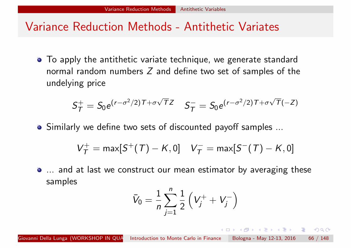
Variance Reduction Methods - Antithetic Variates
To apply the antithetic variate technique, we generate standardnormal random numbers Z and define two set of samples of theundelying price
S+T = S0e(r−σ2/2)T+σ
√TZ S−T = S0e(r−σ2/2)T+σ
√T (−Z)
Similarly we define two sets of discounted payoff samples ...
V +T = max[S+(T )− K , 0] V−T = max[S−(T )− K , 0]
... and at last we construct our mean estimator by averaging thesesamples
V0 =1
n
n∑j=1
1
2
(V +j + V−j
)
Giovanni Della Lunga (WORKSHOP IN QUANTITATIVE FINANCE)Introduction to Monte Carlo in Finance Bologna - May 12-13, 2016 66 / 148

Variance Reduction Methods Moment Matching
Variance Reduction Methods - Moment Matching
Let zi , i = 1, ..., n, denote an independent standard normal randomvector used to drive a simulation.
The sample moments will not exactly match those of the standardnormal. The idea of moment matching is to transform the zi tomatch a finite number of the moments of the underlying population.
For example, the first and second moment of the normal randomnumber can be matched by defining
zi = (zi − z)σzsz
+ µz , i = 1, .....n (7)
where z is the sample mean of the zi and σz is the populationstandard deviation, sz is the sample standard deviation of zi , andµz”¿ is the population mean.
Giovanni Della Lunga (WORKSHOP IN QUANTITATIVE FINANCE)Introduction to Monte Carlo in Finance Bologna - May 12-13, 2016 67 / 148

Multi Asset Path Generation
Outline
1 IntroductionSome Basic IdeasTheoretical Foundations of MonteCarlo Simulations
2 Single Asset Path GenerationDefinitionsExact Solution AdvancementNumerical Integration of SDEThe Brownian Bridge
3 Variance Reduction MethodsAntithetic VariablesMoment Matching
4 Multi Asset Path GenerationCholeski Decomposition
Copula Functions5 Valuation of European Option with
Stochastic VolatilitySquare-Root Diffusion: the CIRModelThe Heston Model
6 Valuation of American Option7 The Hull and White Model8 MCS for CVA Estimation
DefinitionsCVA of a Plain Vanilla Swap: theAnalytical ModelCVA of a Plain Vanilla Swap: theSimulation Approach
Giovanni Della Lunga (WORKSHOP IN QUANTITATIVE FINANCE)Introduction to Monte Carlo in Finance Bologna - May 12-13, 2016 68 / 148

Multi Asset Path Generation Choleski Decomposition
Choleski Decomposition
The Choleski Decomposition makes an appearance in Monte CarloMethods where it is used to simulating systems with correlatedvariables.
Cholesky decomposition is applied to the correlation matrix, providinga lower triangular matrix A, which when applied to a vector ofuncorrelated samples, u, produces the covariance vector of thesystem. Thus it is highly relevant for quantitative trading.
The standard procedure for generating a set of correlated normalrandom variables is through a linear combination of uncorrelatednormal random variables;
Assume we have a set of n independent standard normal randomvariables Z and we want to build a set of n correlated standardnormals Z ′ with correlation matrix Σ
Z ′ = AZ , AAt = Σ
Giovanni Della Lunga (WORKSHOP IN QUANTITATIVE FINANCE)Introduction to Monte Carlo in Finance Bologna - May 12-13, 2016 69 / 148

Multi Asset Path Generation Choleski Decomposition
Choleski Decomposition
We can find a solution for A in the form of a triangular matrixA11 0 . . . 0A21 A22 . . . 0
......
. . . . . .An1 An2 . . . Ann
diagonal elements
aii =
√√√√Σii −i−1∑k=1
a2ik
off-diagonal elements
aij =1
aii
(Σij −
i−1∑k=1
aikajk
)
Giovanni Della Lunga (WORKSHOP IN QUANTITATIVE FINANCE)Introduction to Monte Carlo in Finance Bologna - May 12-13, 2016 70 / 148
Multi Asset Path Generation Choleski Decomposition
Choleski Decomposition
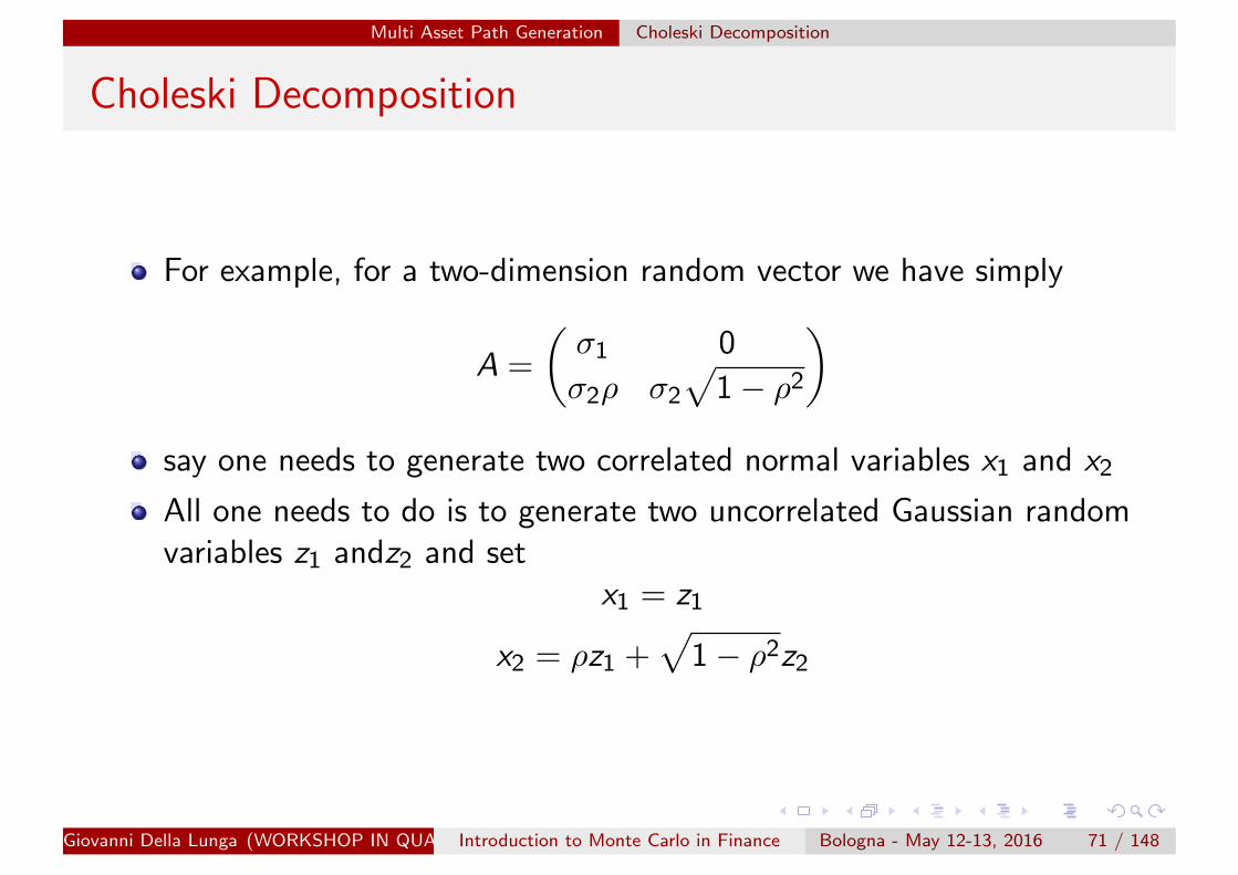
For example, for a two-dimension random vector we have simply
A =
(σ1 0
σ2ρ σ2
√1− ρ2
)say one needs to generate two correlated normal variables x1 and x2
All one needs to do is to generate two uncorrelated Gaussian randomvariables z1 andz2 and set
x1 = z1
x2 = ρz1 +√
1− ρ2z2
Giovanni Della Lunga (WORKSHOP IN QUANTITATIVE FINANCE)Introduction to Monte Carlo in Finance Bologna - May 12-13, 2016 71 / 148

Multi Asset Path Generation Copula Functions
Copula Functions
Why Copula?
A copula is a function that links univariate marginals to theirmultivariate distribution;
Non-linear dependence
Be able to measure dependence for heavy tail distributions
Very flexible: parametric, semi-parametric or non-parametric
Be able to study asymptotic properties of dependence structures
Many others... (ask to Cherubini for everything you would like toknow about copula)
Giovanni Della Lunga (WORKSHOP IN QUANTITATIVE FINANCE)Introduction to Monte Carlo in Finance Bologna - May 12-13, 2016 72 / 148

Multi Asset Path Generation Copula Functions
Copula Functions
In most applications, the distribution is assumed to be a multivariategaussian or a log-normal distribution for tractable calculus, even if thegaussian assumption may not be appropriate.
Copulas are a powerful tool for finance, because the modellingproblem can be splitted into two steps:• the first step deals with the identification of the marginaldistributions;• and the second step consists in defining the appropriate copula inorder to represent the dependence structure in a good manner.
Giovanni Della Lunga (WORKSHOP IN QUANTITATIVE FINANCE)Introduction to Monte Carlo in Finance Bologna - May 12-13, 2016 73 / 148

Multi Asset Path Generation Copula Functions
Copula Functions
Giovanni Della Lunga (WORKSHOP IN QUANTITATIVE FINANCE)Introduction to Monte Carlo in Finance Bologna - May 12-13, 2016 74 / 148

Multi Asset Path Generation Copula Functions
Copula Functions
Giovanni Della Lunga (WORKSHOP IN QUANTITATIVE FINANCE)Introduction to Monte Carlo in Finance Bologna - May 12-13, 2016 75 / 148

Multi Asset Path Generation Copula Functions
Notebook
GitHub : polyhedron-gdl;
Notebook :mcs multi asset path;
Giovanni Della Lunga (WORKSHOP IN QUANTITATIVE FINANCE)Introduction to Monte Carlo in Finance Bologna - May 12-13, 2016 76 / 148

Valuation of European Option with Stochastic Volatility
Outline
1 IntroductionSome Basic IdeasTheoretical Foundations of MonteCarlo Simulations
2 Single Asset Path GenerationDefinitionsExact Solution AdvancementNumerical Integration of SDEThe Brownian Bridge
3 Variance Reduction MethodsAntithetic VariablesMoment Matching
4 Multi Asset Path GenerationCholeski Decomposition
Copula Functions5 Valuation of European Option with
Stochastic VolatilitySquare-Root Diffusion: the CIRModelThe Heston Model
6 Valuation of American Option7 The Hull and White Model8 MCS for CVA Estimation
DefinitionsCVA of a Plain Vanilla Swap: theAnalytical ModelCVA of a Plain Vanilla Swap: theSimulation Approach
Giovanni Della Lunga (WORKSHOP IN QUANTITATIVE FINANCE)Introduction to Monte Carlo in Finance Bologna - May 12-13, 2016 77 / 148
Valuation of European Option with Stochastic Volatility Square-Root Diffusion: the CIR Model
CIR Model
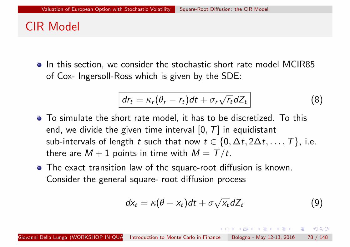
In this section, we consider the stochastic short rate model MCIR85of Cox- Ingersoll-Ross which is given by the SDE:
drt = κr (θr − rt)dt + σr√
rtdZt (8)
To simulate the short rate model, it has to be discretized. To thisend, we divide the given time interval [0,T ] in equidistantsub-intervals of length t such that now t ∈ {0,∆t, 2∆t, . . . ,T}, i.e.there are M + 1 points in time with M = T/t.
The exact transition law of the square-root diffusion is known.Consider the general square- root diffusion process
dxt = κ(θ − xt)dt + σ√
xtdZt (9)
Giovanni Della Lunga (WORKSHOP IN QUANTITATIVE FINANCE)Introduction to Monte Carlo in Finance Bologna - May 12-13, 2016 78 / 148

Valuation of European Option with Stochastic Volatility Square-Root Diffusion: the CIR Model
CIR Model
It can be show that xt , given xs with s = t −∆t, is distributedaccording to
xt =σ2(1− e−κ∆t)
4κχ′2d
(4−κ∆t
σ2(1− e−κ∆t)xs
)where χ′2d denotes a non-central chi-squared random variable with
d =4θκ
σ2
degrees of freedom and non-centrality parameter
l =4−κ∆t
σ2(1− e−κ∆t)xs
Giovanni Della Lunga (WORKSHOP IN QUANTITATIVE FINANCE)Introduction to Monte Carlo in Finance Bologna - May 12-13, 2016 79 / 148

Valuation of European Option with Stochastic Volatility Square-Root Diffusion: the CIR Model
CIR Model
For implementation purposes, it may be convenient to sample achi-squared random variable χ2
d instead of a non-central chi-squaredone, χ′2d .
If d > 1, the following relationship holds true
χ′2d (l) = (z +√
l)2 + χ2d−1
where z is an independent standard normally distributed randomvariable.
Similarly, if d ≤ 1, one has
χ′2d (l) = χ2d+2N
where N is now a Poisson-distributed random variable with intensityl/2. For an algorithmic representation of this simulation scheme referto Glasserman, p. 124.
Giovanni Della Lunga (WORKSHOP IN QUANTITATIVE FINANCE)Introduction to Monte Carlo in Finance Bologna - May 12-13, 2016 80 / 148

Valuation of European Option with Stochastic Volatility Square-Root Diffusion: the CIR Model
CIR Model: Pricing ZCB
A MC estimator for the value of the ZCB at t is derived as follows.
Consider a certain path i of the I simulated paths for the short rateprocess with time grid t ∈ {0,∆t, 2∆t, . . . ,T}.We discount the terminal value of the ZCB, i.e. 1, step-by-stepbackward. For t < T and s = t −∆t we have
Bs,i = Bt,ie− rt+rs
2∆t
The MC estimator of the ZCB value at t is
BMCt =
1
I
I∑i=1
Bt,i
Giovanni Della Lunga (WORKSHOP IN QUANTITATIVE FINANCE)Introduction to Monte Carlo in Finance Bologna - May 12-13, 2016 81 / 148

Valuation of European Option with Stochastic Volatility Square-Root Diffusion: the CIR Model
CIR Model: Pricing ZCB
The present value of the ZCB in the CIR model takes the form:
B0(T ) = b1(T )e−b2(T )r0
where
b1(T ) =
[2γ exp((κr + γ)T/2)
2γ + (κr + γ)(eγT − 1)
] 2κr θrσ2r
b2(T ) =2(eγT − 1)
2γ + (κr + γ)(eγT − 1)
γ =√κ2r + 2σ2
r
Giovanni Della Lunga (WORKSHOP IN QUANTITATIVE FINANCE)Introduction to Monte Carlo in Finance Bologna - May 12-13, 2016 82 / 148

Valuation of European Option with Stochastic Volatility Square-Root Diffusion: the CIR Model
Notebook
GitHub : polyhedron-gdl;
Notebook : n06 mcs cir;
Giovanni Della Lunga (WORKSHOP IN QUANTITATIVE FINANCE)Introduction to Monte Carlo in Finance Bologna - May 12-13, 2016 83 / 148

Valuation of European Option with Stochastic Volatility The Heston Model
The Heston Model
Stochastic volatility models are those in which the variance of astochastic process is itself randomly distributed.The models assumes that the underlying security’s volatility is arandom process, governed by state variables such as the price level ofthe underlying security, the tendency of volatility to revert to somelong-run mean value, and the variance of the volatility process itself,among others.Stochastic volatility models are one approach to resolve ashortcoming of the Black–Scholes model.In particular this model cannot explain long-observed features of theimplied volatility surface such as volatility smile and skew, whichindicate that implied volatility does tend to vary with respect to strikeprice and expiry.By assuming that the volatility of the underlying price is a stochasticprocess rather than a constant, it becomes possible to modelderivatives more accurately.
Giovanni Della Lunga (WORKSHOP IN QUANTITATIVE FINANCE)Introduction to Monte Carlo in Finance Bologna - May 12-13, 2016 84 / 148

Valuation of European Option with Stochastic Volatility The Heston Model
The Heston Model
By assuming that the volatility of the underlying price is a stochasticprocess rather than a constant, it becomes possible to model derivativesmore accurately.
Heston model
CEV model
SABR volatility model
GARCH model
Giovanni Della Lunga (WORKSHOP IN QUANTITATIVE FINANCE)Introduction to Monte Carlo in Finance Bologna - May 12-13, 2016 85 / 148

Valuation of European Option with Stochastic Volatility The Heston Model
The Heston Model
In this section we are going to consider the stochastic volatility modelMH93 with constant short rate.
This section values European call and put options in this model byMCS.
As for the ZCB values, we also have available a semi-analytical pricingformula which generates natural benchmark values against which tocompare the MCS estimates.
Giovanni Della Lunga (WORKSHOP IN QUANTITATIVE FINANCE)Introduction to Monte Carlo in Finance Bologna - May 12-13, 2016 86 / 148

Valuation of European Option with Stochastic Volatility The Heston Model
The Heston Model
The basic Heston model assumes that St , the price of the asset, isdetermined by a stochastic process:
dSt = µSt dt +√νtSt dW S
t
where νt , the instantaneous variance, is a CIR process:
dνt = κ(θ − νt) dt + ξ√νt dW ν
t
and dW St , dW ν
t are Wiener process with correlation ρ, or equivalently,with covariance ρdt.
Giovanni Della Lunga (WORKSHOP IN QUANTITATIVE FINANCE)Introduction to Monte Carlo in Finance Bologna - May 12-13, 2016 87 / 148

Valuation of European Option with Stochastic Volatility The Heston Model
The Heston Model
The parameters in the above equations represent the following:
µ is the rate of return of the asset.
θ is the long variance, or long run average price variance; as t tendsto infinity, the expected value of νt tends to θ.
κ is the rate at which νt reverts to θ.
ξ is the volatility of the volatility, or vol of vol, and determines thevariance of νt .
If the parameters obey the following condition (known as the Fellercondition) then the process νt is strictly positive
2κθ > ξ2
Giovanni Della Lunga (WORKSHOP IN QUANTITATIVE FINANCE)Introduction to Monte Carlo in Finance Bologna - May 12-13, 2016 88 / 148

Valuation of European Option with Stochastic Volatility The Heston Model
The Heston Model
The correlation introduces a new problem dimension into thediscretization for simulation purposes.
To avoid problems arising from correlating normally distributedincrements (of S) with chi-squared distributed increments (of v), wewill in the following only consider Euler schemes for both the S and vprocess.
This has the advantage that the increments of v become normallydistributed as well and can therefore be easily correlated with theincrements of S .
Giovanni Della Lunga (WORKSHOP IN QUANTITATIVE FINANCE)Introduction to Monte Carlo in Finance Bologna - May 12-13, 2016 89 / 148

Valuation of European Option with Stochastic Volatility The Heston Model
The Heston Model
we consider two discretization schemes for S and seven discretizationschemes for v .
For S we have the simple Euler discretization scheme (withs = t −∆t)
St = Ss
(er∆t +
√vt√
∆tz1t
)As an alternative we consider the exact log Euler scheme
St = Sse(r−vt/2)∆t+√vt√
∆tz1t
This one is obtained by considering the dynamics of log St andapplying Ito’s lemma to it.
Giovanni Della Lunga (WORKSHOP IN QUANTITATIVE FINANCE)Introduction to Monte Carlo in Finance Bologna - May 12-13, 2016 90 / 148

Valuation of European Option with Stochastic Volatility The Heston Model
The Heston Model
These schemes can be combined with any of the following Eulerschemes for the square-root diffusion (x+ = max[0, x ]):
Full Truncation
xt = xs + κ(θ − x+s )∆t + σ
√x+s
√∆tzt , xt = x+
t
Partial Truncation
xt = xs + κ(θ − xs)∆t + σ√
x+s
√∆tzt , xt = x+
t
Truncation
xt = max[0, xs + κ(θ − xs)∆t + σ
√xs√
∆tzt]
Reflection
xt = |xs |+ κ(θ − |xs |)∆t + σ√|xs |√
∆tzt , xt = |xt |
Giovanni Della Lunga (WORKSHOP IN QUANTITATIVE FINANCE)Introduction to Monte Carlo in Finance Bologna - May 12-13, 2016 91 / 148

Valuation of European Option with Stochastic Volatility The Heston Model
The Heston Model
Hingham-Mao
xt = xs + κ(θ − xs)∆t + σ√|xs |√
∆tzt , xt = |xt |
Simple Reflection
xt =∣∣∣ xs + κ(θ − xs)∆t + σ
√xs√
∆tzt
∣∣∣Absorption
xt = x+s + κ(θ − x+
s )∆t + σ√
x+s
√∆tzt , xt = x+
t
In the literature there are a lot of tests and numerical studiesavailable that compare efficiency and precision of differentdiscretization schemes.
Giovanni Della Lunga (WORKSHOP IN QUANTITATIVE FINANCE)Introduction to Monte Carlo in Finance Bologna - May 12-13, 2016 92 / 148

Valuation of European Option with Stochastic Volatility The Heston Model
Notebook
GitHub : polyhedron-gdl;
Notebook : n07 mcs heston;
Giovanni Della Lunga (WORKSHOP IN QUANTITATIVE FINANCE)Introduction to Monte Carlo in Finance Bologna - May 12-13, 2016 93 / 148

Valuation of American Option
Outline
1 IntroductionSome Basic IdeasTheoretical Foundations of MonteCarlo Simulations
2 Single Asset Path GenerationDefinitionsExact Solution AdvancementNumerical Integration of SDEThe Brownian Bridge
3 Variance Reduction MethodsAntithetic VariablesMoment Matching
4 Multi Asset Path GenerationCholeski Decomposition
Copula Functions5 Valuation of European Option with
Stochastic VolatilitySquare-Root Diffusion: the CIRModelThe Heston Model
6 Valuation of American Option7 The Hull and White Model8 MCS for CVA Estimation
DefinitionsCVA of a Plain Vanilla Swap: theAnalytical ModelCVA of a Plain Vanilla Swap: theSimulation Approach
Giovanni Della Lunga (WORKSHOP IN QUANTITATIVE FINANCE)Introduction to Monte Carlo in Finance Bologna - May 12-13, 2016 94 / 148

Valuation of American Option
Valuation of American Option by Simulation
As we have seen Monte Carlo simulation is a flexible and powerfulnumerical method to value financial derivatives of any kind.
However being a forward evolving technique, it is per se not suited toaddress the valuation of American or Bermudan options which arevalued in general by backwards induction.
Longstaff and Schwartz provide a numerically efficient method toresolve this problem by what they call Least-Squares Monte Carlo.
The problem with Monte Carlo is that the decision to exercise anAmerican option or not is dependent on the continuation value.
Giovanni Della Lunga (WORKSHOP IN QUANTITATIVE FINANCE)Introduction to Monte Carlo in Finance Bologna - May 12-13, 2016 95 / 148

Valuation of American Option
Valuation of American Option by Simulation
Consider a simulation with M + 1 points in time and I paths.
Given a simulated index level St,i , t ∈ {0, ...,T}, i ∈ {1, ..., I}, what isthe continuation value Ct,i (St,i ), i.e. the expected payoff of notexercising the option?
The approach of Longstaff-Schwartz approximates continuation valuesfor American options in the backwards steps by an ordinaryleast-squares regression.
Equipped with such approximations, the option is exercised if theapproximate continuation value is lower than the value of immediateexercise. Otherwise it is not exercised.
Giovanni Della Lunga (WORKSHOP IN QUANTITATIVE FINANCE)Introduction to Monte Carlo in Finance Bologna - May 12-13, 2016 96 / 148

Valuation of American Option
Valuation of American Option by Simulation
In order to explain the metodology, let’s start from a simpler problem(Gabbriellini, see credits section).
Consider a bermudan option which is similar to an american option,except that it can be early exercised once only on a specific set ofdates.
In the next figure, we can represent the schedule of a put bermudanoption with strike K and maturity in 6 years. Each year you canchoose whether to exercise or not ...
Giovanni Della Lunga (WORKSHOP IN QUANTITATIVE FINANCE)Introduction to Monte Carlo in Finance Bologna - May 12-13, 2016 97 / 148

Valuation of American Option
Valuation of American Option by Simulation
Giovanni Della Lunga (WORKSHOP IN QUANTITATIVE FINANCE)Introduction to Monte Carlo in Finance Bologna - May 12-13, 2016 98 / 148

Valuation of American Option
Valuation of American Option by Simulation
Let’s consider a simpler example: a put option which can be exercisedearly only once ...
Giovanni Della Lunga (WORKSHOP IN QUANTITATIVE FINANCE)Introduction to Monte Carlo in Finance Bologna - May 12-13, 2016 99 / 148

Valuation of American Option
Valuation of American Option by Simulation
Giovanni Della Lunga (WORKSHOP IN QUANTITATIVE FINANCE)Introduction to Monte Carlo in Finance Bologna - May 12-13, 2016 100 / 148

Valuation of American Option
Valuation of American Option by Simulation
Can we price this product by means of a Monte Carlo? Yes we can!Let’s see how.
Let’s implement a MC which actually simulates, besides the evolutionof the market, what an investor holding this option would do (clearlyan investor who lives in the risk neutral world). In the followingexample we will assume the following data, S(T ) =, K =, r =, σ =,t1 = 1y , T = 2y .
We simulate that 1y has passed, computing the new value of theasset and the new value of the money market account
S(t1 = 1y) = S(t0)e(r− 12σ2)(t1−t0)+σ
√t1−t0N(0,1)
B(t1 = 1y) = B(t0)er(t1−t0)
Giovanni Della Lunga (WORKSHOP IN QUANTITATIVE FINANCE)Introduction to Monte Carlo in Finance Bologna - May 12-13, 2016 101 / 148

Valuation of American Option
Valuation of American Option by Simulation
At this point the investor could exercise. How does he know if it isconvenient?
In case of exercise he knows exactly the payoff he’s getting.
In case he continues, he knows that it is the same of having aEuropean Put Option.
So, in mathematical terms we have the following payoff in t1
max [K − S(t1),P(t1,T ; S(t1),K )]
where P(t1,T ; S(t1),K ) is the price of a Put which we computeanalytically! In the jargon of american products, P is called thecontinuation value, i.e. the value of holding the option instead ofearly exercising it.
Giovanni Della Lunga (WORKSHOP IN QUANTITATIVE FINANCE)Introduction to Monte Carlo in Finance Bologna - May 12-13, 2016 102 / 148

Valuation of American Option
Valuation of American Option by Simulation
So the premium of the option is the average of this discounted payoffcalculated in each iteration of the Monte Carlo procedure.
1
N
∑i
max [K − Si (t1),P(t1,T ; Si (t1),K )]
Some considerations are in order.
We could have priced this product because we have an analyticalpricing formula for the put. What if we didn’t have it?
Giovanni Della Lunga (WORKSHOP IN QUANTITATIVE FINANCE)Introduction to Monte Carlo in Finance Bologna - May 12-13, 2016 103 / 148

Valuation of American Option
Valuation of American Option by Simulation
Brute force solution: for each realization of S(t1) we run anotherMonte Carlo to price the put.
This method (called Nested Monte Carlo) is very time consuming.For this very simple case it’s time of execution grows as N2, whichbecomes prohibitive when you deal with more than one exercise date!
Let’s search for a finer solution analyzing the relationship between thecontinuation value (in this very simple example) and the simulatedrealization of S at step t1.
let’s plot the discounted payoff at maturity, Pi , versus Si (t1) ...
Giovanni Della Lunga (WORKSHOP IN QUANTITATIVE FINANCE)Introduction to Monte Carlo in Finance Bologna - May 12-13, 2016 104 / 148

Valuation of American Option
Valuation of American Option by Simulation
Giovanni Della Lunga (WORKSHOP IN QUANTITATIVE FINANCE)Introduction to Monte Carlo in Finance Bologna - May 12-13, 2016 105 / 148

Valuation of American Option
Valuation of American Option by Simulation
Giovanni Della Lunga (WORKSHOP IN QUANTITATIVE FINANCE)Introduction to Monte Carlo in Finance Bologna - May 12-13, 2016 106 / 148

Valuation of American Option
As you can see, the analytical price of the put is a curve which kindsof interpolate the cloud of Monte Carlo points.
This suggest us that the price at time t1 can be computed by meansof an average on all discounted payoff (i.e. the barycentre of thecloud made of discounted payoff)
So maybe... the future value of an option can be seen as the problemof finding the curve that best fits the cloud of discounted payoff (upto date of interest)!!!
In the next slide, for example, there is a curve found by means of alinear regression on a polynomial of 5th order...
Giovanni Della Lunga (WORKSHOP IN QUANTITATIVE FINANCE)Introduction to Monte Carlo in Finance Bologna - May 12-13, 2016 107 / 148

Valuation of American Option
Valuation of American Option by Simulation
Giovanni Della Lunga (WORKSHOP IN QUANTITATIVE FINANCE)Introduction to Monte Carlo in Finance Bologna - May 12-13, 2016 108 / 148

Valuation of American Option
Valuation of American Option by Simulation
Giovanni Della Lunga (WORKSHOP IN QUANTITATIVE FINANCE)Introduction to Monte Carlo in Finance Bologna - May 12-13, 2016 109 / 148

Valuation of American Option
Valuation of American Option by Simulation
We now have an empirical pricing formula for the put to be used inmy MCS
P(t1,T ,S(t1),K) = c0 + c1S(t1) + c2S(t1)2 + c3S(t1)3 + c4S(t1)4 + c5S(t1)5
The formula is obviously fast, the cost of the algorithm being the bestfit.
Please note that we could have used any form for the curve (not onlya plynomial).
This method has the advantage that it can be solved as a linearregression, which is fast.
Giovanni Della Lunga (WORKSHOP IN QUANTITATIVE FINANCE)Introduction to Monte Carlo in Finance Bologna - May 12-13, 2016 110 / 148

Valuation of American Option
The Longstaff-Schwartz Algorithm
The major insight of Longstaff-Schwartz is to estimate thecontinuation value Ct,i by ordinary least-squares regression, thereforethe name ”Least Square Monte Carlo” for their algorithm;
They propose to regress the I continuation values Yt,i against the Isimulated index levels St,i .
Given D basis functions b with b1, . . . , bD : RD → R for theregression, the continuation value Ct,i is according to their approachapproximated by:
Giovanni Della Lunga (WORKSHOP IN QUANTITATIVE FINANCE)Introduction to Monte Carlo in Finance Bologna - May 12-13, 2016 111 / 148

Valuation of American Option
The Longstaff-Schwartz Algorithm
Given D basis functions b with b1, . . . , bD : RD → R for theregression, the continuation value Ct,i is according to their approachapproximated by:
Ct,i =D∑
d=1
α?d ,tbd(St,i ) (1)
The optimal regression parameters α?d ,t are the result of theminimization
minα1,t ,...,αD,t
1
I
I∑i=1
(Yt,i −
D∑d=1
αd ,tbd(St,i )
)2
Giovanni Della Lunga (WORKSHOP IN QUANTITATIVE FINANCE)Introduction to Monte Carlo in Finance Bologna - May 12-13, 2016 112 / 148

Valuation of American Option
The Longstaff-Schwartz Algorithm
Simulate I index level paths with M + 1 points in time leading toindex level values St,i , t ∈ {0, ...,T}, i ∈ {1, ..., I};For t = T the option value is VT ,i = hT (ST ,i ) by arbitrageStart iterating backwards t = T −∆t, . . . ,∆t:
regress the Tt,i against the St,i , i ∈ {1, . . . , I}, given D basis function b
approximate Ct,i by Ct,i according to (1) given the optimal parametersα?d,t from (2)set
Vt,i =
{ht(St,i ) if ht(St,i ) > Ct,i exercise takes place
Yt,i if ht(St,i ) ≤ Ct,i no exercise takes place
repeat iteration steps until t = ∆t;
for t = 0 calculate the LSM estimator
V LSM0 = e−r∆t 1
I
I∑i=1
V∆t,i
Giovanni Della Lunga (WORKSHOP IN QUANTITATIVE FINANCE)Introduction to Monte Carlo in Finance Bologna - May 12-13, 2016 113 / 148

Valuation of American Option
Notebook
GitHub : polyhedron-gdl;
Notebook : mcs american;
Giovanni Della Lunga (WORKSHOP IN QUANTITATIVE FINANCE)Introduction to Monte Carlo in Finance Bologna - May 12-13, 2016 114 / 148

The Hull and White Model
Outline
1 IntroductionSome Basic IdeasTheoretical Foundations of MonteCarlo Simulations
2 Single Asset Path GenerationDefinitionsExact Solution AdvancementNumerical Integration of SDEThe Brownian Bridge
3 Variance Reduction MethodsAntithetic VariablesMoment Matching
4 Multi Asset Path GenerationCholeski Decomposition
Copula Functions5 Valuation of European Option with
Stochastic VolatilitySquare-Root Diffusion: the CIRModelThe Heston Model
6 Valuation of American Option7 The Hull and White Model8 MCS for CVA Estimation
DefinitionsCVA of a Plain Vanilla Swap: theAnalytical ModelCVA of a Plain Vanilla Swap: theSimulation Approach
Giovanni Della Lunga (WORKSHOP IN QUANTITATIVE FINANCE)Introduction to Monte Carlo in Finance Bologna - May 12-13, 2016 115 / 148

The Hull and White Model
Hull-White Model
Described by the SDE for the short rate
dr = (θ(t)− ar)dt + σdw (10)
See Brigo-Mercurio ...
Our version simplified: a and σ constant;
AKA Extended Vasicek (Note: r(t) is Gaussian);
θ determined uniquely by term structure;
Giovanni Della Lunga (WORKSHOP IN QUANTITATIVE FINANCE)Introduction to Monte Carlo in Finance Bologna - May 12-13, 2016 116 / 148

The Hull and White Model
Hull-White Model: Solving for r(t)
d(eatr) = eatdr + aeatrdt = θ(t)eat + eatσdw
integrating both sides we obtain
eatr(t) = r(0) +
t∫0
θ(s)easds + σ
t∫0
easdw(s)
simplify
r(t) = r(0)e−at +
t∫0
θ(s)e−a(t−s)ds + σ
t∫0
e−a(t−s)dw(s)
Giovanni Della Lunga (WORKSHOP IN QUANTITATIVE FINANCE)Introduction to Monte Carlo in Finance Bologna - May 12-13, 2016 117 / 148

The Hull and White Model
Hull-White Model: Solving for P(t,T)
P(t,T ) = V (t, r(t)) where V solves the PDE
Vt + (θ(t)− ar)Vr +1
2σ2Vrr − rV = 0
Final-time condition V (T , r) = 1 for all r at t = T ;
Ansatz:V = A(t,T )e−B(t,T )r(t)
A and B must satisfy:
At − θ(t)AB +1
2σ2(AB)2 = 0, and Bt − aB + 1 = 0
Final-time conditions
A(T ,T ) = 1 and B(T ,T ) = 0
Giovanni Della Lunga (WORKSHOP IN QUANTITATIVE FINANCE)Introduction to Monte Carlo in Finance Bologna - May 12-13, 2016 118 / 148

The Hull and White Model
Hull-White Model: Solving for P(t,T)
B independent of θ so
B(t,T ) =1
a
(1− e−a(T−t)
)(11)
Solving for A requires integration of θ
A(t,T ) = exp
− T∫t
θ(s)B(s,T )ds − σ2
2a2(B(t,T )− T + t)− σ2
4aB(t,T )2
Giovanni Della Lunga (WORKSHOP IN QUANTITATIVE FINANCE)Introduction to Monte Carlo in Finance Bologna - May 12-13, 2016 119 / 148

The Hull and White Model
Hull-White Model: Determining θ
Determining θ from the term structure at time 0;
Goal: demonstrate the relation
θ(t) =∂f
f ∂T(0, t) + af (0, t) +
σ2
2a(1− e−2at) (12)
Recallf (t,T ) = −∂ log P(t,T )/∂T
Giovanni Della Lunga (WORKSHOP IN QUANTITATIVE FINANCE)Introduction to Monte Carlo in Finance Bologna - May 12-13, 2016 120 / 148

The Hull and White Model
Hull-White Model: Determining θ
We have
− logP(0,T ) =
T∫0
θ(s)B(s,T )ds +σ2
2a2[B(0,T )− T ] +
σ2
4aB(0,T )2 + B(0,T )r0
Differentiating and using that B(T ,T ) = 1 and ∂TB − 1 = −aB weget
f (0,T ) =
T∫0
θ(s)∂TB(s,T )ds− σ2
2a2B(0,T )+
σ2
2a2B(0,T )∂TB(0,T )+∂TB(0,T )r0
Giovanni Della Lunga (WORKSHOP IN QUANTITATIVE FINANCE)Introduction to Monte Carlo in Finance Bologna - May 12-13, 2016 121 / 148

The Hull and White Model
Hull-White Model: Determining θ
Differentiating again, get:
∂T f (0,T ) = θ(T ) +
T∫0
θ(s)∂TTB(s,T )ds
− σ2
2a2∂TB(0,T )
+σ2
2a2[(∂TB(0,T ))2 + B(0,T )∂TTB(0,T )]
+ ∂TTB(0,T )r0
(13)
Giovanni Della Lunga (WORKSHOP IN QUANTITATIVE FINANCE)Introduction to Monte Carlo in Finance Bologna - May 12-13, 2016 122 / 148

The Hull and White Model
Hull-White Model: Determining θ
Combine these equations, and use a∂TB + ∂TTB = 0;
Get:
af (0,T ) + ∂T f (0,T ) = θ(T )− σ2
2a(aB + ∂TB) +
σ2
2a[aB∂TB + (∂TB)2 + B∂TTB]
Substitute formula for B and simplify to get
af (0,T ) + ∂T f (0,T ) = θ(T )− σ2
2a(1− e−2aT )
QED
Giovanni Della Lunga (WORKSHOP IN QUANTITATIVE FINANCE)Introduction to Monte Carlo in Finance Bologna - May 12-13, 2016 123 / 148

The Hull and White Model
Additive Factor Gaussian Model
The model is given by dynamics (Brigo-Mercurio p. 143):
r(t) = x(t) + φ(t)
wheredx(t) = −ax(t)dt + σdWt x(0) = 0
and φ is a deterministic shift which is added in order to fit exactly theinitial zero coupon curve
Giovanni Della Lunga (WORKSHOP IN QUANTITATIVE FINANCE)Introduction to Monte Carlo in Finance Bologna - May 12-13, 2016 124 / 148

The Hull and White Model
Additive Factor Gaussian Model
So the short rate r(t) is distributed normally with mean and variancegiven by (Brigo-Mercurio p.144 equations 4.6 with η = 0)
E (rt |rs) = x(s)e−a(t−s) + φ(t)
Var(rt |rs) =σ2
2a
(1− e−2a(t−s)
)where φ(T ) = f M(0,T ) + σ2
2a
(1− e−aT
)2and f M(0,T ) is the
market instantaneous forward rate at time t as seen at time 0.
Giovanni Della Lunga (WORKSHOP IN QUANTITATIVE FINANCE)Introduction to Monte Carlo in Finance Bologna - May 12-13, 2016 125 / 148

The Hull and White Model
Additive Factor Gaussian Model
Model discount factors are calculated as in Brigo-Mercurio (section4.2):
P(t,T ) =PM(0,T )
PM(0, t)exp (A(t,T ))
A(t,T ) =1
2[V (t,T )− V (0,T ) + V (0, t)]− 1− e−a(T−t)
ax(t)
where
V (t,T ) =σ2
a2
[T − t +
2
ae−a(T−t) − 1
2ae−2a(T−t) − 3
2a
]
Giovanni Della Lunga (WORKSHOP IN QUANTITATIVE FINANCE)Introduction to Monte Carlo in Finance Bologna - May 12-13, 2016 126 / 148
MCS for CVA Estimation
Outline
1 IntroductionSome Basic IdeasTheoretical Foundations of MonteCarlo Simulations
2 Single Asset Path GenerationDefinitionsExact Solution AdvancementNumerical Integration of SDEThe Brownian Bridge
3 Variance Reduction MethodsAntithetic VariablesMoment Matching
4 Multi Asset Path GenerationCholeski Decomposition
Copula Functions5 Valuation of European Option with
Stochastic VolatilitySquare-Root Diffusion: the CIRModelThe Heston Model
6 Valuation of American Option7 The Hull and White Model8 MCS for CVA Estimation
DefinitionsCVA of a Plain Vanilla Swap: theAnalytical ModelCVA of a Plain Vanilla Swap: theSimulation Approach
Giovanni Della Lunga (WORKSHOP IN QUANTITATIVE FINANCE)Introduction to Monte Carlo in Finance Bologna - May 12-13, 2016 127 / 148

MCS for CVA Estimation Definitions
CVA Context
Counterparty risk can be considered broadly from two different pointsof view;
The first point of view is risk management, leading to capitalrequirements revision, trading limits discussions and so on;
The second point of view is valuation or pricing, leading to amountscalled Credit Valuation Adjustment (CVA) and extensions thereof,including netting, collateral, re-hypothecation, close-out specification,wrong way risk and funding cost;
Giovanni Della Lunga (WORKSHOP IN QUANTITATIVE FINANCE)Introduction to Monte Carlo in Finance Bologna - May 12-13, 2016 128 / 148

MCS for CVA Estimation Definitions
Exposure Profiles
There are two main effects that determine the credit exposure overtime for a single transaction or for a portfolio of transactions with thesame counterparty: diffusion and amortization;
as time passes, the ”diffusion effect” tends to increase the exposure,since there is greater variability and, hence, greater potential formarket price factors to move significantly away fro current levels;
the ”amortization effect”, in contrast, tends to decrease the exposureover time, because it reduces the remaining cash flows that areexposed to default;
Giovanni Della Lunga (WORKSHOP IN QUANTITATIVE FINANCE)Introduction to Monte Carlo in Finance Bologna - May 12-13, 2016 129 / 148

MCS for CVA Estimation Definitions
Exposure Profiles
For single cash flow products, such as FX Forwards, the potentialexposure peaks at the maturity of the transaction, because it is drivenpurely by ”diffusion effect”;
on the other hand, for products with multiple cash flows, such asinterest-rate swaps, the potential exposure usually peaks at one-thirdto one-half of the way into the life of the transaction;
Giovanni Della Lunga (WORKSHOP IN QUANTITATIVE FINANCE)Introduction to Monte Carlo in Finance Bologna - May 12-13, 2016 130 / 148

MCS for CVA Estimation Definitions
Credit Value Adjustment
Credit Value Adjustment (CVA) is by definition the differencebetween the risk-free portfolio value and the true portfolio value thattakes into account the possibility of a counterparty’s default;
in other words CVA is the market value of counterparty credit risk;
Giovanni Della Lunga (WORKSHOP IN QUANTITATIVE FINANCE)Introduction to Monte Carlo in Finance Bologna - May 12-13, 2016 131 / 148
MCS for CVA Estimation Definitions
Credit Value Adjustment
Assuming independence between exposure and counterparty’s creditquality greatly simplifies the analysis.
under this assumption we can write
CVA = (1− R)
T∫0
EE ?(t)dPD(0, t) (14)
where EE ?(t) is the risk-neutral discounted expected exposure (EE)given by
EE ?(t) = EQ
[B0
BtE (t)
](15)
Giovanni Della Lunga (WORKSHOP IN QUANTITATIVE FINANCE)Introduction to Monte Carlo in Finance Bologna - May 12-13, 2016 132 / 148

MCS for CVA Estimation Definitions
Credit Value Adjustment
In general calculating discounted EE requires simulations;
Exposure is simulated at a fixed set of simulation dates, therefore theintegral in (14) has to be approximated by the sum:
CVA = (1− R)N∑i=1
EE ?(tk)PD(tk−1, tk) (16)
Since expectation in (15) is risk-neutral, scenario models for all pricefactors should be arbitrage free;
This is achieved by appropriate calibration of drifts and volatilitiesspecified in the price-factor evolution model;
Giovanni Della Lunga (WORKSHOP IN QUANTITATIVE FINANCE)Introduction to Monte Carlo in Finance Bologna - May 12-13, 2016 133 / 148

MCS for CVA Estimation CVA of a Plain Vanilla Swap: the Analytical Model
The General Unilateral Counterparty Risk Pricing Formula
At valuation time t, and provided the counterparty has not defaultedbefore t, i.e. on {τ > t}, the price of our payoff with maturity Tunder counterparty risk is
Et [Π(t,T )] = Et [Π(t,T )]− Et [LGD It≤τ≤TD(t, τ)(NPV (τ))+]︸ ︷︷ ︸positive counterparty-risk adjustment
= Et [Π(t,T )]− UCVA(t,T )
(17)
with
UCVA(t,T ) = Et [LGD It≤τ≤TD(t, τ)(NPV (τ))+]
= Et [LGD It≤τ≤TD(t, τ)EAD](18)
Where LGD = 1− REC is the loss given default, and the recoveryfraction REC is assumed to be deterministic.
Giovanni Della Lunga (WORKSHOP IN QUANTITATIVE FINANCE)Introduction to Monte Carlo in Finance Bologna - May 12-13, 2016 134 / 148

MCS for CVA Estimation CVA of a Plain Vanilla Swap: the Analytical Model
The General Unilateral Counterparty Risk Pricing Formula
It is clear that the value of a defaultable claim is the sum of the valueof the corresponding default-free claim minus a positive adjustment.
The positive adjustment to be subtracted is called (Unilateral) CreditValuation Adjustment (CVA), and it is given by a call option (withzero strike) on the residual NPV at default, giving nonzerocontribution only in scenario where τ ≤ T .
Giovanni Della Lunga (WORKSHOP IN QUANTITATIVE FINANCE)Introduction to Monte Carlo in Finance Bologna - May 12-13, 2016 135 / 148

MCS for CVA Estimation CVA of a Plain Vanilla Swap: the Analytical Model
The General Unilateral Counterparty Risk Pricing Formula
Counterparty risk thus adds and optionality level to the original payoff.
This renders the counterparty risk payoff model dependent even whenthe original payoff is model independent.
This implies, for example, that while the valuation of swaps withoutcounterparty risk is model independent, requiring no dynamical modelfor the term structure (no volatility and correlations in particular), thevaluation of swaps under counterpaty risk will require and interestrate model.
Giovanni Della Lunga (WORKSHOP IN QUANTITATIVE FINANCE)Introduction to Monte Carlo in Finance Bologna - May 12-13, 2016 136 / 148

MCS for CVA Estimation CVA of a Plain Vanilla Swap: the Analytical Model
The General Unilateral Counterparty Risk Pricing Formula
Now we explore the well known result that the component of the IRSprice due to counterparty risk is the sum of swaption prices withdifferent maturities, each weighted with the probability of defaultingaround that maturity.
Let us suppose that we are a default free counterparty ”B” entering apayer swap with a defaultable counterparty ”C”, exchanging fixed forfloating payments at times Ta+1, . . . ,Tb.
Denote by βi the year fraction between Ti−1 and Ti , and by P(t,Ti )the default-free zero coupon bond price at time t for maturity Ti . Wetake a unit notional on the swap.
The contract requires us to pay a fixed rate K and to receive thefloating rate L resetting one period earlier until the default time τ of”B” or until final maturity T if τ > T .
The fair forward-swap rate K at a given time t in a default-freemarket is the one which renders the swap zero-valued in t.
Giovanni Della Lunga (WORKSHOP IN QUANTITATIVE FINANCE)Introduction to Monte Carlo in Finance Bologna - May 12-13, 2016 137 / 148

MCS for CVA Estimation CVA of a Plain Vanilla Swap: the Analytical Model
The General Unilateral Counterparty Risk Pricing Formula
In the risk-free case the discounted payoff for a payer IRS is
b∑i=a+1
D(t,Ti )βi (L(Ti−1,Ti )− K ) (19)
and the forward swap rate rendering the contract fair is
K = S(t; Ta,Tb) = Sa,b(t) =P(t,Ta)− P(t,Tb)
b∑i=a+1
P(t,Ti )βi
Giovanni Della Lunga (WORKSHOP IN QUANTITATIVE FINANCE)Introduction to Monte Carlo in Finance Bologna - May 12-13, 2016 138 / 148
MCS for CVA Estimation CVA of a Plain Vanilla Swap: the Analytical Model
The General Unilateral Counterparty Risk Pricing Formula
Of course if we consider the possibility that ”C” may default, thecorrect spread to be paid in the fixed leg is lower as we are willing tobe rewarded for bearing this default risk.
In particular we have
UCVA(t,Tb) = LGD Et [Iτ≤TbD(t, τ)(NPV (τ))+]
= LGD
Tb∫Ta
PS (t; s,Tb,K ,S(t; s,Tb), σs,Tb) dsQ{τ ≤ s}
(20)
being PS (t; s,Tb,K , S(t; s,Tb), σs,Tb) the price in t of a swaption
with maturity s, strike K underlying forward swap rate S(t; s,Tb),volatility σs,Tb
and underlying swap with final maturity Tb.
Giovanni Della Lunga (WORKSHOP IN QUANTITATIVE FINANCE)Introduction to Monte Carlo in Finance Bologna - May 12-13, 2016 139 / 148

MCS for CVA Estimation CVA of a Plain Vanilla Swap: the Analytical Model
The General Unilateral Counterparty Risk Pricing Formula
The proof is the following: given independence between τ and theinterest rates, and given that the residual NPV is a forward start IRSstarting at the default time, the option on the residual NPV is a sumof swaptions with maturities ranging the possible values of the defaulttime, each weighted (thanks to the independence assumption) by theprobabilities of defaulting around each time value.
We can simplify formulas allow the default to happen only at pointsTi of the fixed leg payment grid.
In this way the expected loss part is simplified.
Giovanni Della Lunga (WORKSHOP IN QUANTITATIVE FINANCE)Introduction to Monte Carlo in Finance Bologna - May 12-13, 2016 140 / 148
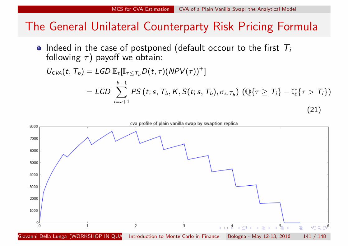
MCS for CVA Estimation CVA of a Plain Vanilla Swap: the Analytical Model
The General Unilateral Counterparty Risk Pricing Formula
Indeed in the case of postponed (default occour to the first Tifollowing τ) payoff we obtain:
UCVA(t,Tb) = LGD Et [Iτ≤TbD(t, τ)(NPV (τ))+]
= LGDb−1∑i=a+1
PS (t; s,Tb,K , S(t; s,Tb), σs,Tb ) (Q{τ ≥ Ti} −Q{τ > Ti})
(21)
Giovanni Della Lunga (WORKSHOP IN QUANTITATIVE FINANCE)Introduction to Monte Carlo in Finance Bologna - May 12-13, 2016 141 / 148

MCS for CVA Estimation CVA of a Plain Vanilla Swap: the Analytical Model
Notebook
GitHub : polyhedron-gdl;
Notebook : n09 cva swap;
Giovanni Della Lunga (WORKSHOP IN QUANTITATIVE FINANCE)Introduction to Monte Carlo in Finance Bologna - May 12-13, 2016 142 / 148

MCS for CVA Estimation CVA of a Plain Vanilla Swap: the Simulation Approach
CVA of a Plain Vanilla Swap: the Simulation Approach
1 Simulate yield curve at future dates
2 Calculate your derivatives portfolio NPV (net present value) at eachtime point for each scenario
3 Calculate CVA as sum of Expected Exposure multiplied by probabilityof default at this interval
CVA = (1− R)
∫DF (t)EE (t)dQt
where R is the Recovery Rate (normally set to 40%) EE (t) is theexpected exposure at time t and dQt the survival probability density,DF (t) is the discount factor at time t.
Giovanni Della Lunga (WORKSHOP IN QUANTITATIVE FINANCE)Introduction to Monte Carlo in Finance Bologna - May 12-13, 2016 143 / 148

MCS for CVA Estimation CVA of a Plain Vanilla Swap: the Simulation Approach
CVA of a Plain Vanilla Swap: the Simulation Approach
In this simple example we will use a modified version of Hull Whitemodel to generate future yield curves. In practice many banks usesome yield curve evolution models based on this model.
For each point of time we will generate whole yield curve based onshort rate. Then we will price our interest rate swap on each of thesecurves;
To approximate CVA we will use BASEL III formula for regulatorycapital charge approximating default probability [or survivalprobability ] as exp(−ST/(1− R)) so we get
CVA = (1− R)∑i
EE(Ti )? + EE(T ?
i−1
2
(e−S(Ti−1)/(1−R) − e−S(Ti )/(1−R)
)where EE ? is the discounted Expected Exposure of portfolio.
Giovanni Della Lunga (WORKSHOP IN QUANTITATIVE FINANCE)Introduction to Monte Carlo in Finance Bologna - May 12-13, 2016 144 / 148

MCS for CVA Estimation CVA of a Plain Vanilla Swap: the Simulation Approach
CVA of a Plain Vanilla Swap: the Simulation Approach
Giovanni Della Lunga (WORKSHOP IN QUANTITATIVE FINANCE)Introduction to Monte Carlo in Finance Bologna - May 12-13, 2016 145 / 148

MCS for CVA Estimation CVA of a Plain Vanilla Swap: the Simulation Approach
Notebook
GitHub : polyhedron-gdl;
Notebook :n10 mcs cva swap;
Giovanni Della Lunga (WORKSHOP IN QUANTITATIVE FINANCE)Introduction to Monte Carlo in Finance Bologna - May 12-13, 2016 146 / 148

MCS for CVA Estimation CVA of a Plain Vanilla Swap: the Simulation Approach
Credits
Damiano Brigo, Fabio Mercurio ”Interest Rate Models — Theory andPractice” Springer Finance (2006)
Damiano Brigo, Massimo Morini, Andrea Pallavicini ”CounterpartyCredit Risk, Collateral and Funding” Wiley Finance (2013)
Umberto Cherubini, Elisa Luciano, Walter Vecchiato ”CopulaMethods in Finance” Wiley Finance (2004)
Tommaso Gabbriellini ”American Options with Monte Carlo”Presentation on Slideshare
Yves Hilpisch ”Derivatives Analytics with Python” Wiley Finance(2015)
Don L. McLeish ”Monte Carlo Simulation and Finance” WileyFinance (2005)
Giovanni Della Lunga (WORKSHOP IN QUANTITATIVE FINANCE)Introduction to Monte Carlo in Finance Bologna - May 12-13, 2016 147 / 148