UNIT – 1

INTRODUCTION AND OVERVIEW

1.1 Concept of System

Simulation is the representation of a real life system by another system, which

depicts the important characteristics of the real system and allows experimentation on it.

In other words, simulation is an imitation of the reality.

A system is defined as an aggregation or assemblage of objects joined in some

regular interaction or independence.

As an example of a conceptually simple system, consider an aircraft flying under

the control of an autopilot. A gyroscope in the autopilot detects the difference between

the actual heading and the desired heading. It sends the signal to move the control

surfaces. In response to the control surface movement the airframe steers toward the

desired heading.

Desired Heading

Actual Heading

As a second example, consider a factory that makes and assembles parts into a

product. Two major components of the system are the fabrication department making the

part and the assembly department producing the products. A purchasing department

maintains a supply of raw materials and a shipping department dispatches the finished

products. A production control department receives orders and assigns work to the other

departments.

Customer Orders

Raw Finished

Materials Products

Gyroscope Control Surfaces Airframe

Production

control Dept.

Purchasing

Dept

Fabrication

Dept

Assembly

Dept

Shipping

Dept

One more example of system can be taken of an engine governor, which is

required to keep the speed constant within limits, at varying loads of the engine. As the

load is changed, the speed changes, governor balls lift or lower the sleeve, which controls

the fuel supply and in turn speed. It is an automatic control system.

Load

In looking at these systems we see that there are certain distinct objects, each of

which possesses properties of interest. There are also certain interactions occurring in the

system that cause changes in the system.

In case of governor system, the components of the system, the engine, governor,

fuel pump, etc. are all physical. Their relationships are based on well-known physical

laws. Such systems are called physical systems.

The production system, on the other hand comprises of a large number of

departments, with manmade inter-relationships which cannot be represented by physical

objects. Such systems are called non-physical systems. Management systems, social

system, political system, education system etc. are all non-physical systems.

1.2 System Environment

The behavior of one component of a system affects the performance of other

components due to interconnections and hence, when a system is identified it has to be

described and studied as a whole. This methodology of tackling the system is called systems

approach. We may also call it scientific approach. The term system engineering has been

used for engineering employing systems approach.

A system is often affected by changes occurring outside the system. Some system

activities may also produce changes that do not react on the system. Such changes occurring

Engine

(Speed)

Governor (Lift

of sleeve)

Fuel Pump (Control of

Fuel Supply)

outside the system are said to occur in system environment. An important step in modeling

systems is to decide upon the boundary between the system and its environment. The

decision may depend upon the purpose of the study.

In the case of the factory system, for example, the factors controlling the arrival

of orders may be considered to be outside the influence of the factory and therefore part of

the environment. However, if the effect of supply on demand is to be considered, there will

be a relationship between factory output and arrival of orders, and this relationship must be

considered an activity of the system.

Similarly, in the case of a bank system, there may be a limit on the maximum

interest rate that can be paid. For the study of a single bank, this would be regarded as a

constraint imposed by the environment. In a study of the effects of monetary laws on the

banking industry, however, the setting of the limit would be an activity of system.

Another example would be if in a manufacturing system the effect of a particular

work place lay out is to be studied then, activities like inspection, purchasing, packaging, in

process inventory level etc., are all external to the system. On the other hand if the idle time

of bank teller is to be studied, the arrival of customers is an activity internal to the system.

The term endogenous is used to describe activities occurring within the system

and the term exogenous is used to describe activities in the environment that affect the

system. A system for which there is no exogenous activity is said to be a closed system in

contrast to an open system which does have exogenous activities.

1.3 Elements of system

The term entity is used to denote a distinct object of interest in a particular

investigation in system.

The term attribute denotes a property of interest of an entity. There can be many

attributes to a given entity

The term activity is defined as any process that causes changes in the system.

The term event is defined as the different process or operations that take place in

the system.

The terms state or state of the system or state variables is used to mean a

description of all the entities, attributes and activities as they exist at one point in time.

The table 1.1 below lists the examples of entities, attributes, activities, events and

state variables for a few systems. This table does not show a complete list of all entities,

activities, events or states of the system, as the complete list can be made only when the

system is properly defined.

System Entities Attributes Activities Events State Variables

Banking Customers Balance,

Credit, status

Making

deposits,

withdrawals

Arrivals,

departures

Number of

customers

waiting, number

of busy tellers

Traffic control

lights

Vehicles Distance,

speed, type of

vehicles

Driving Stopping,

Starting

Status of traffic

signal, number

waiting, time to

green

Production Machines,

Work Pieces

Processing

rates,

breakdown

times

Machining,

welding,

sampling,

moving of

work pieces

Work arrives

at machine,

processing

starts, ends

Machine busy,

work piece

waiting, machine

down

Super Market Customers,

trolleys,

baskets

Shopping list Collecting

items, checking

out

Arrival in

store, collect

basket, end

shopping

Availability of

stock, variety,

number of

shoppers waiting

for check out

Communication Messages Length,

priority,

destination

Transmitting Sending time,

arrival at

destination

Messages waiting

to be transmitted

Some other terms which are frequently encountered while dealing with a system,

are given below.

Queue: It is a situation, where entities wait for something to happen. It may be

physical queue of people, or of objects, or a list of tasks to be performed.

Creating: Creating is causing an arrival of a new entity to the system at some

point in time.

Scheduling: Scheduling is the process of assigning events to the existing entities,

like the service begin and service and times.

Random Variables: It is a variable with uncertain magnitude, i.e., whose

quantitative value changes at random. The inter arrival times of vehicles arriving at a

petrol pump, or the life of electric bulbs are random variables.

Random Variate: It is a variable generated by using random numbers along with

its probability density function.

Distribution: It is a mathematical law which governs and defines probabilistic

features of the random variables. It is also called probability density function.

Let us take the example of a petrol pump, where vehicles arrive at random for

getting petrol or diesel. In this case,

Entities - vehicles which will comprise of various types of four, three and two

wheelers.

Events – arrival of vehicles, service beginning, service ending, departure of

vehicles

States or state variables – the number of vehicles in the system at a particular

time, number of vehicles waiting, number of workers busy, etc.

Attributes – Type of vehicle i.e. four wheeler, two wheeler, petrol or diesel, size

of fuel tank, filing rate of machine, etc.

Queue – Vehicles waiting in front of the pump.

Random Variables – Inter arrival times of vehicles, service times and billing

times, etc.

Distribution – The distribution may be one of the many statistical probability

density functions. It is generally assumed to be exponential in case of queuing systems.

1.4 System Modeling

A model is defined as the body of information about a system gathered for the

purpose of studying the system. In the case of a physical model, the information in

embodied in the properties of the model, in contrast to the symbolic representation in a

mathematical model. A model is not only as substitute for a system, it is also a

simplification of the system.

The task of deriving a model of a system may be divided broadly into two

subtasks:

1. Establishing the model structure

2. Supplying the data

Establishing the structure determines the system boundary and identifies the

entities, attributes and activities of the system. The data provide the values the attributes

can have and define the relationships involved in the activities. Assumptions about the

system direct the gathering of data, and analysis of the data confirms or refutes the

assumptions. Quite often, the data gathered will disclose an unsuspected relationship

that changes the model structure.

1.5 Types of Models

The models used for the analysis of various types of systems have been classified

in a number of ways, as shown in fig

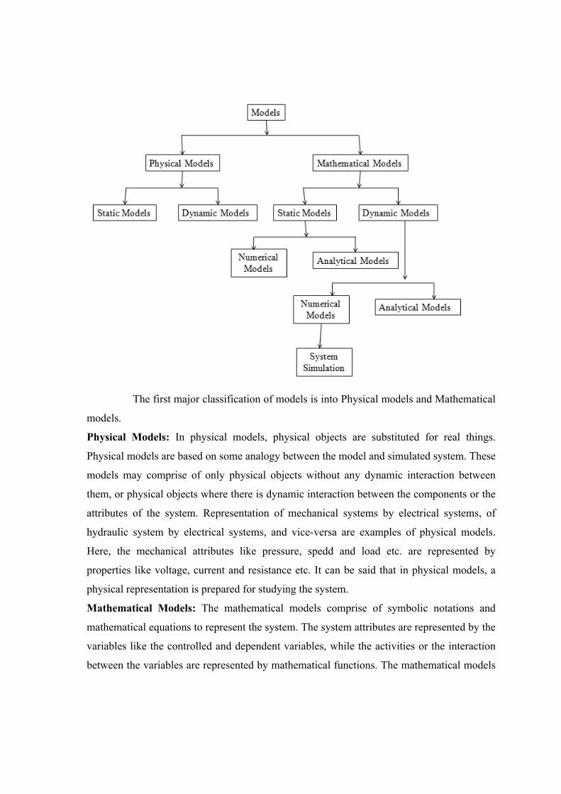
The first major classification of models is into Physical models and Mathematical

models.

Physical Models: In physical models, physical objects are substituted for real things.

Physical models are based on some analogy between the model and simulated system. These

models may comprise of only physical objects without any dynamic interaction between

them, or physical objects where there is dynamic interaction between the components or the

attributes of the system. Representation of mechanical systems by electrical systems, of

hydraulic system by electrical systems, and vice-versa are examples of physical models.

Here, the mechanical attributes like pressure, spedd and load etc. are represented by

properties like voltage, current and resistance etc. It can be said that in physical models, a

physical representation is prepared for studying the system.

Mathematical Models: The mathematical models comprise of symbolic notations and

mathematical equations to represent the system. The system attributes are represented by the

variables like the controlled and dependent variables, while the activities or the interaction

between the variables are represented by mathematical functions. The mathematical models

can be static as well as dynamic and further analytical, numerical or simulation models,

depending upon the techniques employed to find its solution.

Static Models: A static model represents a system, which does not change with

time or represents a system at a particular point in time. Static models describe a system

mathematically, in terms of equations, where the potential effect of each alternative is

ascertained by a single computation of the equation. The variables used in the computations

are averages. The performance of the system is determined by summing the individual

effects.

Since the static models ignore the time dependent variables, these cannot be used

to determine the influence of changes which occur due to the variations in the parameters of

the system. The static models, do not take into consideration the synergy of the components

of the system, where the action of separate elements can have a different effect on the

modeled system than the sum of their individual effect could indicate.

Dynamic Models: The dynamic simulation models represent systems as they

change over time. Dynamic modeling is a software representation of the dynamic or time-

based behavior of a system. While a static model is a mathematical model and involves a

single set of computations of the equations, the dynamic model involves an interactive

procedure of solution. Dynamic model constantly re-computes its equations as the variation

in parameters occur with time.

Dynamic models can predict the performance of the system for a number of

alternative courses of action and can take into consideration the variance or randomness.

Most of the activities occurring in nature are random, their occurrence cannot be controlled,

but dynamic models help to predict the outcome of their behavior.

Analytical and Numerical Models: The classification of models into analytical

and numerical models is based only on the methodology to solve the mathematical model.

The mathematical models which can be solved by employing analytical techniques of

mathematics are called analytical models, while the models which require the application of

numerical methods are called numerical models. The numerical techniques involve the

application of computational procedures to solve the mathematical equations which can be

handles only by computers. The numerical computations in the interactive form are akin to

simulation. Simulation is though used in regard to physical models also, but most of the

applications have been found in mathematical modeling and further for modeling the

dynamic and stochastic behavior of systems.

Deterministic and Stochastic Models:

Deterministic Models: The deterministic models have a known set of inputs,

which result into a unique set of outputs. In case of pure pursuit problem, the initial position

of the target and pursuer, their speeds and the path of flight are known and can be expressed

by mathematical equations. For a given set of inputs there can be only one output. This

model is deterministic. Occurrence of the events is certain and not dependent on chance.

Stochastic Models: In stochastic simulation models, there are one or more

random input variables, which lead to random outputs. The outputs in such a case are only

estimates of true characteristics of the system. The working of a production line, where the

operation times at different work station are random is a stochastic process. The random

variables in a stochastic system may be represented by a continuous probability function or

theses may be totally discrete. Depending upon the distribution of random variables,

stochastic models can be further divided into continuous models and discrete models.

Because of the randomness of the variables, the results of stochastic simulations are always

approximate. To obtain reliable results, a stochastic simulation model has to be run for a

sufficiently long duration

1.6 System Simulation:

Forming of a physical model and experimenting on it is simulation. Developing a

mathematical model and deriving information by analytical means is simulation. Where

analytical methods are not applicable numerical methods or specific algorithms are applied

to analyze the mathematical models, which again is simulation. These models, physical as

well as mathematical can be of variety of types. Thus the term simulation described as a

procedure of establishing a model and deriving solution from it covers the whole gamut of

physical, analogue, analytical and numerical investigations. To distinguish this

interpretation of simulation from more general used of technique the term system simulation

is defined as

“The technique of solving problems by observation of the performance, over

time, of a dynamic model of the system”

Thus the dynamic model and time element are two important components of

system simulation. In many simulations, the time element may not be significant parameter.

System behavior may not be a function of time, but still the system is analyzed by step-by-

step calculations of the successive stages of the system.

For example, the size of a repair crew for maintaining a fixed fleet of buses is to

be determined. Size of the repair crew, in this case will be a step or interval in the step-by-

step analysis of the system.

1.7 Simulation – A Management Laboratory:

The technique of system simulation is a very important tool of decision making.

The managerial problems are generally too complex to be solved by the analytical

techniques. Various techniques of operations research are applicable to only specific types of

situations, and require many assumptions and simplifications to be made for fitting the

problem into the model. Many of the events occurring in real systems are random with

intricate interrelationships, with their solution beyond the scope of standard probability

analysis. Under the circumstances, simulation is the only tool, which allows the management

to test the various alternative strategies. Since, simulation is a sort of experimentation, and

when used for analyzing managerial problems, it is rightly called the management laboratory.

For training the business executives, simulations called management games are used in many

universities and management institutes.

Comparison of Simulation and Analytical Methods

In contrast to analytical, models, the simulations are “run” rather than solved.

Running a simulation is like conducting an experiment and an experiment always gives

specific solutions depending upon the input conditions and characteristics of the system,

while the analytical methods give general solutions. For example in an optimization

problem, the mathematical model will give optimum value in a single solution and in

case of simulation model a number of simulations will have to be executed, each

resulting in a different value, one of which will approximate the optimum value.

The results obtained by simulation are approximate while the results obtained by

analytical methods are exact. To increase the reliability of simulation results, simulation

has to be run for longer periods. However in case of complex situation, mathematical

modeling becomes difficult and many assumptions and simplifications have to made for

constructing the model. In such cases, the analytical model may give highly approximate

or unrealistic results. It is a question of judgment up to what level the system has to be

approximated or abstracted to fit a mathematical model.

The accuracy of simulation results depends upon the level of details at which the

mode has been developed. More detailed is the model, more complex is its construction.

More detailed simulation mode requires greater time and effort to construct the model

and its execution takes longer run time. Thus a compromise has to be made for the level

of detail, to obtain reasonably realistic results.

The mathematical models can handle only a limited range of problems, while

simulation can handle all sorts of problems. It is said that when every method fails,

simulation can be employed to solve the problem.

When to use simulation:

1. Simulation is very useful for experiments with internal interactions of a

complex system, or of a subsystem within a complex system.

2. Simulation can be employed to experiment with new designs and policies,

before implementing them.

3. Simulation can be used to verify the results obtained by analytical methods

and to reinforce the analytical techniques.

4. Simulation is very useful in determining the influence of changes in input

variables on the output of the system

5. Simulation helps is suggesting modifications in the system under investigation

for its optimal performance

Steps in Simulation Study:

1. Problem formulation

2. Model construction

3. Data collection

4. Model programming

5. Validation

6. Design of experiment

7. Simulation run and analysis

8. Documentation

9. Implementation

Problem formulation: The clear and unambiguous description of the problem, definition of the

objectives of the study, identification of alternatives to be considered and methodology for

evaluation the effectiveness of these alternatives needs to be stated at the beginning of any study.

If the statement of the problem is provided by the policy makers, the analyst must ensure that the

problem being describes is clearly understood. Alternatively, if the problem statement is being

formulated by the analyst, the policy makers should be able to understand it and accept it. At this

stage, it should also be ascertained whether the simulation technique is the appropriate tool for

solving problem. The overall plan should include a statement of the alternative systems to be

considered, the measures of performance to be used, the methodologies of analysis to be used,

and the anticipated result of the study.

Model Construction: The model building is much of an art than science. There are no standard

rules for building a successful and appropriate model for all types of situations. There are only

certain guidelines, which can be followed. The art of modeling is enhanced by the ability to

abstract the essential features of the system, to select and modify the basic assumptions and

simplifications that characterize the system, and then improve and elaborate the model. To start

with a simple model is constructed, which is modified step-by-step, every time enriching and

elaborating its characteristics, to achieve an appropriate model, which meets the desired

objectives. In some situations, building block method is employed, where the blocks of

components of system are built and validated. These blocks are then combined to obtain model

for the complete system.

Data Collection: The availability of input data about the system is essential for the construction

of its model. The kind of data to be collected depends upon the objectives of the study, the

required data may be available as past history, or may have to be collected. The construction of

the simulation model and the collection of data have a constant interplay, and the type and

amount of data required may change as the model develops. The data is required not only as an

input to the model, but also some data is used to validate the simulation model. Since data

collection generally takes longer time, it should be started as early as possible.

Model Programming: Any simulation model worth the name requires enormous amount of

computations and information storage, which is possible only with the use of high speed

computers. The translation of model into a computer recognizable format is termed as

programming. Many general and special purpose simulation languages and special purpose and

problem specific simulation softwares are developed which can be used for simulation modeling.

It is for the modeler to decide, whether a simulation language is to be used or special purpose

software is to be used.

Validation: It is essential to ensure that the model is an accurate representation of the system,

which has been modeled. That the computer program performs properly and the results obtained

are identical to the ones from the real system. Validation involves both the validation of the logic

and accuracy of programming. This requires step-by-step modification of the model. It is rarely

possible to develop a reasonably large simulation model in its entirety in first step. Good deal of

debugging is required. The validation is thus an iterative process of comparing the model to

actual system behavior, identifying the discrepancies, applying corrections and again comparing

the performance. This process continues till a model of desired accuracy is obtained. The data

collected from the system is of great help in validation of the model.

Design of Experiment: The simulation is basically experimentation of the model of the system

under investigation. Simulation experiment in most of the situations involves stochastic

variables, which result into stochastic results. The average values of result obtained may not be

of desired reliability. To make the results meaningful it is essential that simulation experiment be

designed in such a way that results obtained are within some specified tolerance limits and at a

reasonable level of confidence. Decisions regarding the length of simulation run, initial

conditions, removal of initial bias, and number of replications of each run; use of variance

reduction techniques etc. has to be made.

Simulation Run and Analysis: The simulation program is run as per the simulation design; the

results are obtained and analyzed, to estimate the measures of performance of the system. Based

on the results, a decision is made, whether or not any modification in the design of simulation

experiment is needed. This step is a sort validation of the simulation design. It may reveal that

more runs or more replications are required.

Documentation: Documentation of a simulation program is necessary as the program can be

used by the same or different analyst in future. The program can be used with modifications for

some other identical situation, which can be facilitated if the program is adequately documented.

Documentation of the simulation model, allows the user to change parameters of the model at

will to investigate the influence on outputs, to find optimal combinations. The program should be

documented in such a way that a new analyst can easily understand it.

Implementation: There will not be any problems in the implementation of the simulation

program, if the user is fully conversant with the model, and understands the nature of its inputs

and outputs and underlying assumptions. Thus, it is important that the model user is involved in

the development of the simulation model from the very first step.

1.8 Advantages of simulation:

1. Simulation helps to learn about a real system, without having the system at all. For

example, the wind tunnel testing of the model of an aero plane does not require a full

sized plane.

2. Many managerial decision making problems are too complex to be solved by

mathematical programming

3. In many situations, experimenting with an actual system may not be possible at all. For

example, it is not possible to conduct experiment, to study the behavior of a man on the

surface of moon. In some other situations, even if experimentation is possible, it may be

too costly or risky

4. In the real system, the changes we want to study may take place too slowly or too fast to

be observed conveniently. Computer simulation can compress the performance of a

system over years into a few minutes of computer running time. Conversely, in systems

like nuclear reactors where millions of events take place per second, simulation can

expand the time required level.

5. Through simulation, management can foresee the difficulties and bottlenecks, which may

come up due to the introduction of new machines, equipments and processes. It thus

eliminates the need of costly trial and error method of trying out the new concepts.

6. Simulation being relatively free from mathematics can easily be understood by the

operation personnel and non-technical managers. This helps in getting the proposed plans

accepted and implemented.

7. Simulation models are comparatively flexible and can be modified to accommodate the

changing environment to the real situation.

8. Simulation technique is easier to use than the mathematical models, and can be used for a

wide range of situations.

9. Extensive computer software packages are available, making it very convenient to use

fairly sophisticated simulation models.

10. Simulation is a very good tool of training and has advantageously been used for training

the operating and managerial staff in the operation of complex systems. Space engineers

simulate space flights in laboratories to train the future astronauts for working in

weightless environments. Airplane pilots are given extensive training on flight

simulators, before they are allowed to handle real aeroplanes.

Limitations of Simulation Techniques:

1. Simulation does not produce optimum results. When the model deals with uncertainties,

the results of simulation are only reliable estimates subject to statistical errors.

2. Quantification of the variables is another difficulty. In a number of situations, it is not

possible to quantify all the variables that affect the behavior of the system.

3. In very large and complex problems, the large number of variables, and the inter-

relationships between them make the problem very unwieldy

4. Simulation is by no means a cheap method of analysis. Even small simulations take

considerable computer time. In a number of situations, simulation is comparatively

costlier and time consuming.

5. Other important limitation stem from too much tendency to rely on the simulation

models. This results in applications of the technique to some simple situations, which can

more appropriately be handled by other techniques of mathematical programming.

Areas of Applications

1. Manufacturing: Design analysis and optimization of production system, materials

management, capacity planning, layout planning and performance evaluation, evaluation

of process quality

2. Business: Market analysis, prediction of consumer behavior, optimization of marketing

strategy and logistics, comparative evaluation of marketing campaigns.

3. Military: Testing of alternative combat strategies, air operations, sea operations,

simulated war exercises, practicing ordinance effectiveness, and inventory management.

4. Healthcare applications: Such as planning of health services, expected patient density,

facilities requirement, hospital staffing, and estimation the effectiveness of a health care

program.

5. Communication applications: Such as network design and optimization, evaluating

network reliability, manpower planning, sizing of message buffers.

6. Computer applications: Such as designing hardware configurations and operating system

protocols, sharing and networking.

7. Economic applications: Such as portfolio management, forecasting impact of Govt.

policies and international market fluctuations on the economy, budgeting and forecasting

market fluctuations.

8. Transport applications: Design and testing of alternative transportation policies,

transportation networks - roads, railways, airways etc., evaluation of timetables, traffic

planning.

9. Environment applications: Solid waste management, performance evaluation of

environment programs, evaluation of pollution control systems.

10. Biological applications: Such as population genetics and spread of epidemics.

1.8 Continuous and Discreet Systems:

From the viewpoint of simulation, the systems are usually classified into two

categories:

Continuous systems

Discrete systems

Continuous Systems: Systems in which the state of the system changes continuously

with time are called continuous systems. The pure pursuit problem which represents a

continuous system since the state variables, the locations of target and pursuer, varies

continuously with time. Generally the systems in which the relationships can be

expressed by mathematical expressions as in engineering and physical sciences turn out

to be discreet systems. In continuous systems, the variables are by and large

deterministic.

Discrete Systems: Systems in which the state changes abruptly at discrete points in time

are called discrete systems. The inventory system and queuing systems are examples of

discrete systems. In inventory system, the demand of items as well as the replenishment

of the stock occurs at discrete points in time and also in discrete numbers. Similarly in

case of queuing systems the customers arrive and leave the system at discrete points in

time. Generally the systems encountered in operations research and management sciences

are discreet systems. The variables in discrete systems generally deal with stochastic

situations.

There are also systems that are intrinsically continuous but information about

them is only available at discrete points in time. These are called sampled-data systems.

The study of such systems includes the problem of determining the effects of the discrete

sampling, especially when the intention is to control the system on the basis of

information gathered by the sampling.

1.9 Monte – Carlo Method

The term ‘Monte Carlo Method’ is a very general term and the Monte Carlo

Methods are used widely varying from economics to nuclear physics to waiting lines and to

regulating the flow of traffic etc. Monte Carlo methods are stochastic techniques and make

use of random numbers and probability statistics to solve the problems. The way this

technique is applied varies from field to field and problem to problem. Monte Carlo method

is applied to solve both deterministic as well as stochastic problems. There are many

deterministic problems also which are solved by using random numbers and interactive

procedure of calculations. In such a case we convert the deterministic model into a stochastic

model, and the results obtained are not exact values, but only estimates. (Examples:D S Hira)