introduction to microeconomics - middlesex … workbook.pdfintroduction to microeconomics | p a g e...
TRANSCRIPT
2014
Working the Basics
By Fred J. Colangelo Professor of Business and Economics
Middlesex Community College
Introduction to Microeconomics
| P a g e 1
Creative Commons public licenses provide a standard set of terms and conditions that creators and other rights holders may use to share original works of authorship and other material subject to
copyright and certain other rights specified in the public license below. The following considerations are for informational purposes only, are not exhaustive, and do not form part of our licenses.
You are free to:
Share — copy and redistribute the material in any medium or format.
The licensor cannot revoke these freedoms as long as you follow the license terms.
Under the following terms:
Attribution — You MUST give appropriate credit, provide a link to the license, and indicate if changes were made. You may do so in any reasonable manner, but not in any way that suggests the licensor endorses you or your use.
NonCommercial — You may NOT use the material for commercial purposes.
NoDerivatives — If you remix, transform, or build upon the material; you may NOT distribute the modified material.
No additional restrictions — You may NOT apply legal terms or technological measures that legally restrict others from doing anything the license permits.
P a g e 2 |
Microeconomics is the branch of economics that analyzes the market behavior of consumers and firms in an attempt to understand the decision-making process of firms and households. Microeconomics is concerned with the interaction between individual buyers and sellers and the factors that influence the choices made by buyers and sellers. In particular, microeconomics focuses on patterns of supply and demand and the determinations of price and output in individual markets.
This textbook is an interactive workbook that will help student master the basic concepts of microeconomics that they would encounter in a microeconomics class. The workbook consists of seven chapters where the student will be required to perform basic fundamental exercises using pencil and eraser to help them master the basic concepts of supply and demand, shifts in supply and demand, equilibrium, elasticity, externalities, public finance, tax systems, consumer choice, production and costs topics such as total and marginal revenue.
Chapter 1: Supply and Demand .......................................................... 2
Chapter 2: Equilibrium ..................................................................... 13
Chapter 3: Elasticity ......................................................................... 19
Chapter 4: Externalities .................................................................... 22
Chapter 5: Public Finance and Choice .............................................. 30
Chapter 6: Consumer Choice ............................................................ 35
Chapter 7: Production and Cost ....................................................... 41
| P a g e 3
Chapter 1 – Supply & DemandIn the world of economics, behaviors of buyers and sellers are important. Buyers determine the demand side of the market; they include consumers who purchase goods and services. Sellers on the other hand determine the supply side of the market; they produce and sell goods and services. The interface between buyers and sellers determines what the market prices will be and amounts that will be supplied to the market through the forces of supply and demand.
The lessons of supply and demand can be applied to many different types of problems. The law of demand states that when the price of a good or service falls the quantity demanded increases and when the price of a good or service rises the quantity demanded decreases as long as all things remain equal, ceteris paribus. The formula used to determine how this happens is shown below.
P ↑ ⇒ QD ↓ and P ↓ ⇒ QD ↑ This chapter will contain a series of four working exercises with various scenarios to help reinforce the student’s understanding on how supply and demand work. These exercises include the topics:
o Supply Schedules
o Supply Curves
o Demand Curves
o Demand Shifts
o Supply Shifts

P a g e 4 |
Exercise 1 This exercise is designed to help reinforce the student’s understanding of the topic of Supply and Demand. This exercise can be used in conjunction with any economics textbook that addresses this topic.
NOTE: As you are working through each scenario in this exercise make sure that you label all parts of your diagrams to avoid mistakes. This exercise should be done using a ruler if necessary so that your lines are accurate and pencil and eraser so that you can make changes if you make a mistake. Do not use pen!
Firms supplying goods want to maximize their profits; the higher the price of their product per unit the greater the profitability. When price is low and expenses high companies are less profitable and they will generally produce less. The following is individual supply information for Frank and Company. At $5.00 per pound Frank and Company would be able to supply seven hundred pounds of coffee per month, the rest of the producers 5300, at $4.00 supply of six hundred pounds; the rest of the producers 4400, at $3.00 supply of five hundred pounds, the rest of the producers 3500, and at $2.00 two hundred pounds, the rest of the producers 2800. Any price $2.00 or less company will lose money. In the space to the right create Supply Schedule for Franks and Company and a Market Supply Schedule.
Using the blank graph to the right create an Individual Supply Curve for Frank and Company based on the information provided above in Scenario 1.
PR
ICE
QUANTITY

| P a g e 5
Using the blank graph to the right to create a Market Supply Curve based on the information provided above in the in Scenario 1.
PR
ICE
QUANTITY

P a g e 6 |
This exercise is designed to help reinforce the student’s understanding of the topic of Supply and Demand. This exercise can be used in conjunction with any economics textbook that addresses this topic
NOTE: As you are working through each scenario in this exercise make sure that you label all parts of your diagrams to avoid mistakes. This exercise should be done using a ruler if necessary so that your lines are accurate and pencil and eraser so that you can make changes if you make a mistake. Do not use pen!
The following provides Jonathans Soup Kitchen supply
demands for peanuts that he would serve each month
at his church’s soup kitchen before dinner in the
upcoming year.
At $6.00 per pound Jonathans Soup Kitchen would be
able to purchase five pounds of peanuts per month, at
$5.00 six pounds; at $4.00 eight pounds; at $3.00 ten
pounds; and at $1.00 twelve pounds. In the space to the
right create Jonathan’s Soup Kitchen Demand Schedule
for Peanuts.
Using the blank graph to the right and the information
provided in Scenario #1, create an Individual Demand
Curve for Jonathans Soup Kitchen peanut requirements
for the upcoming month.
PR
ICE
QUANTITY

| P a g e 7
What would be the Market Supply Schedule if the
remaining churches in the Jonathans Soup Kitchen
geographical area were to purchase fifty pounds at $6.00
per pound; sixty pounds at $5.00 per pound; seventy
pounds at $4.00 per pound; eighty pounds at $3.00 per
pound; and one hundred pounds at $1.00 per pound? In
the space to the right, create a Market Demand Schedule
for Peanuts.
Make sure that you include all market information as you
need to create a complete schedule.
Using the blank graph to the right, create a Market
Demand Curve for peanuts based on the information
provided in the above in Scenario #3.
PR
ICE
QUANTITY

P a g e 8 |
Use the graph to the right to answer each of the following questions. In the spaces provided indicate whether the movement is a shift or change in demand /supply.
1. A movement from A to B represents ___________ in ___________.
2. A movement from A to T represents a ___________ in ___________.
3. A movement from B to A represents ___________ in ___________.
4. A movement from T to A represents a ___________ in ___________.
PR
ICE
S1
S2
A
B
T
QUANTITY
Use the graph to the right to answer each of the following questions. In the spaces provided indicate whether the movement is a shift or change in demand /supply.
1. A movement from C to D represents ___________ in ___________.
2. A movement from Z to C represents a ___________ in ___________.
3. A movement from D to C represents ___________ in ___________.
4. A movement from C to Z represents a ___________
in ___________.
PR
ICE
D1
D2
D
C
Z
QUANTITY

| P a g e 9
This exercise is designed to help reinforce the student’s understanding of the topic of Shifts in Supply and Demand. This exercise can be used in conjunction with any economics textbook that addresses this topic.
NOTE: As you are working through each scenario in this exercise make sure that you label all parts of your diagrams to avoid mistakes. This exercise should be done using a ruler if necessary so that your lines are accurate and pencil and eraser so that you can make changes if you make a mistake. Do not use pen!
Use the blank graph to the right to help determine the possible Shift In Demand if the taste for Starbucks coffee was changed but did not improve its taste in fact it was
worse. Show the direction of your movement using
arrow for positive shifts and arrow for negative shifts. Also draw the new demand curve. Briefly explain why this might happen.
PR
ICE
D1
QUANTITY
Use the blank graph to the right to help determine the possible Shift In Demand if income increases and you are dealing with a normal good. Show the direction of your
movement using arrow for positive shifts and arrow for negative shifts. Also draw the new demand curve. Briefly explain why this might happen.
PR
ICE
D1
QUANTITY

P a g e 1 0 |
Use the blank graph to the right to help determine the possible Shift In Demand if income increases and you are dealing with an inferior good. Show the direction of your
movement using arrow for positive shifts and arrow for negative shifts. Also draw the new demand curve. Briefly explain why this might happen.
PR
ICE
D1
QUANTITY
Use the blank graph to the right to help determine the possible Shift In Demand for a high end product in Detroit if there is a major layoff at the Ford Plant. Show the
direction of your movement using arrow for positive
shifts and arrow for negative shifts. Also draw the new demand curve. Briefly explain why this might happen.
PR
ICE
D1
QUANTITY

| P a g e 1 1
Use the blank graph to the right to help determine the possible Shift In Demand if the number of buyers increases in a particular market. Show the direction of your
movement using arrow for positive shifts and arrow for negative shifts. Also draw the new demand curve. Briefly explain why this might happen.
PR
ICE
D1
QUANTITY
Use the blank graph to the right to help determine the possible Shift In Demand if a future price increase is
expected. Show the direction of your movement using
arrow for positive shifts and arrow for negative shifts. Also draw the new demand curve. Briefly explain why this might happen.
PR
ICE
D1
QUANTITY
P a g e 1 2 |
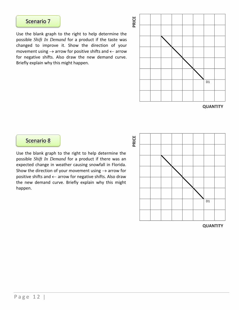
Use the blank graph to the right to help determine the possible Shift In Demand for a product if the taste was changed to improve it. Show the direction of your
movement using arrow for positive shifts and arrow for negative shifts. Also draw the new demand curve. Briefly explain why this might happen.
PR
ICE
D1
QUANTITY
Use the blank graph to the right to help determine the possible Shift In Demand for a product if there was an expected change in weather causing snowfall in Florida.
Show the direction of your movement using arrow for
positive shifts and arrow for negative shifts. Also draw the new demand curve. Briefly explain why this might happen.
PR
ICE
D1
QUANTITY

| P a g e 1 3
This exercise is designed to help reinforce the student’s understanding of the topic of supply shifts. This exercise can be used in conjunction with any economics textbook that addresses this topic.
NOTE: As you are working through each scenario in this exercise make sure that you label all parts of your diagrams to avoid mistakes. This exercise should be done using a ruler if necessary so that your lines are accurate and pencil and eraser so that you can make changes if you make a mistake. Do not use pen!
The Orange Patch Farm (OPF) is a grower of oranges and
pumpkins. The following provides what Orange Patch
Farm would supply for orange juice based on the following
prices. At $1.00 per gallon OPF would supply ten thousand
gallons of orange juice per season, at $1.50 per gallon OPF
would supply fifteen thousand gallons of orange juice per
season, at $2.00 per gallon OPF would supply twenty
thousand gallons of orange juice per season, and at $3.00
per gallon OPF would supply thirty thousand gallons of
orange juice per season. Create an OPF Individual Supply
Curve to the right.
PR
ICE
QUANTITY
The following provides what Other Producers (OP) would
supply for orange juice based on the following prices. At
$1.00 per gallon OP would supply a hundred thousand
gallons of orange juice per season, at $1.50 per gallon OP
would supply one hundred and fifty thousand gallons of
orange juice per season, at $2.00 per gallon OP would
supply two hundred thousand gallons of orange juice per
season, at $3.00 per gallon OP would supply three hundred
thousand gallons of orange juice per season. In the space to
the right create a Market Supply Schedule for OJ.

P a g e 1 4 |
Chapter 2 - Equilibrium As determinants of supply or demand change due to factors such as input prices, prices of similar products, the number of suppliers in a market, consumer expectations, and and changes in technology, the supply/demand curves will shift which cause changes in the equilibrium price and equilibrium quantity. Shifts could be positive shift which would move and supply or demand curve to the right or a negative shift which would move and supply or demand curve to the left. Some shifts could be a combination of large and small together which could cause changes to equilibrium.
This chapter will contain a series of two working exercises with various scenarios to help reinforce the student’s understanding on how equilibrium works. These exercises include the topics:
o Combined Shifts
o Simultaneous Changes in Supply and Demand
o Equilibrium Quantity and Demand

| P a g e 1 5
This exercise is designed to help reinforce the student’s understanding of the topic of shifts in equilibrium. This exercise can be used in conjunction with any economics textbook that addresses this topic.
NOTE: As you are working through each scenario in this exercise make sure that you label all parts of your diagrams to avoid mistakes. This exercise should be done using a ruler if necessary so that your lines are accurate and pencil and eraser so that you can make changes if you make a mistake. Do not use pen!
Use the diagram to the right to illustrate your answer.
1. Using the graph show simultaneous changes in supply and demand by using a LARGE increase in supply and a SMALL increase in demand.
A. Describe what happens to the price?
Answer: _______________________
B. Describe what happens to the quantity?
Answer: _______________________ P
RIC
E
QUANTITY
Use the diagram to the right to illustrate your answer.
1. Using the graph show simultaneous changes in supply and demand, with a SMALL increase in supply and a LARGE increase in demand.
A. Describe what happens to the price?
Answer: _______________________
B. Describe what happens to the quantity?
Answer: _______________________
PR
ICE
QUANTITY
P a g e 1 6 |
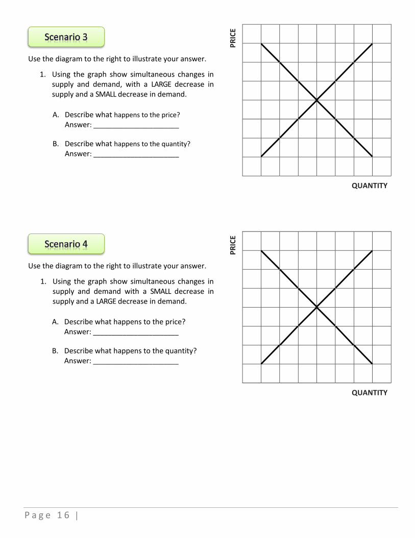
Use the diagram to the right to illustrate your answer.
1. Using the graph show simultaneous changes in supply and demand, with a LARGE decrease in supply and a SMALL decrease in demand.
A. Describe what happens to the price?
Answer: _______________________
B. Describe what happens to the quantity?
Answer: _______________________
PR
ICE
QUANTITY
Use the diagram to the right to illustrate your answer.
1. Using the graph show simultaneous changes in supply and demand with a SMALL decrease in supply and a LARGE decrease in demand.
A. Describe what happens to the price?
Answer: _______________________
B. Describe what happens to the quantity?
Answer: _______________________
PR
ICE
QUANTITY

| P a g e 1 7
Use the diagram to the right to illustrate your answer.
1. Using the graph show simultaneous changes in supply and demand with a SMALL decrease in supply and a SMALL decrease in demand.
A. Describe what happens to the price?
Answer: _______________________
B. Describe what happens to the quantity?
Answer: _______________________
PR
ICE
QUANTITY
Use the diagram to the right to illustrate your answer.
1. Using the graph show simultaneous changes in supply and demand with a SMALL decrease in supply and a NO CHANGE in demand.
A. Describe what happens to the price?
Answer: _______________________
B. Describe what happens to the quantity?
Answer: _______________________
PR
ICE
QUANTITY

P a g e 1 8 |
This exercise is designed to help reinforce the student’s understanding of the topic of shifts in equilibrium. This exercise can be used in conjunction with any economics textbook that addresses this topic.
NOTE: As you are working through each scenario in this exercise make sure that you label all parts of your diagrams to avoid mistakes. This exercise should be done using a ruler if necessary so that your lines are accurate and pencil and eraser so that you can make changes if you make a mistake. Do not use pen!
The diagram to the right shows the supply and demand
curves for SUV’s in a particular geographical area.
Assume that all SUV’s sell for the same market-
determined price. The diagram shows factors that
might cause a shift in the supply and demand curves.
What would be the equilibrium price of an SUV in this
market be?
__________ per sedan
What would be the equilibrium quantity for SUV’s
bought and sold?
__________ per month
PR
ICE
(in
th
ou
san
ds)
30
20
10
100 200 300 400 500 600
QUANTITY (in thousands)
Suppose that the price of an SUV was $35,000. In this case, there would be _____________ which would exert _____________ pressure on prices.
A. A. Shortage (excess demand) of 100 SUV’s per month; upward
B. Shortage (excess demand) of 400 SUV’s per month; upward
C. Surplus (excess supply) of 400 SUV’s per month; downward
D. Shortage (excess supply) of 500 SUV’s per month; downward
How much was the demand? __________
Suppose that the price of an SUV was $15,000.
In this case, there would be _____________ which would exert _____________ pressure on prices.
A. Shortage (excess demand) of 400 SUV’s per month; upward
B. Shortage (excess demand) of 300 SUV’s per month; upward
C. Surplus (excess demand) of 500 SUV’s per month; downward
| P a g e 1 9
D. Surplus (excess supply) of 500 SUV’s per month; downward
How much was supplied? __________
Suppose that the price of an SUV was $40,000.
In this case, there would be _____________ which would exert _____________ pressure on prices.
A. Shortage (excess demand) of 100 SUV’s per month; upward
B. Shortage (excess demand) of 300 SUV’s per month; upward
C. Surplus (excess demand) of 500 SUV’s per month; downward
D. Surplus (excess supply) of 600 SUV’s per month; downward
How much was the demand? __________
Suppose that the price of an SUV was $20,000.
In this case, there would be _____________ which would exert _____________ pressure on prices.
A. Shortage (excess demand) of 100 SUV’s per month; upward
B. Shortage (excess demand) of 200 SUV’s per month; upward
C. Surplus (excess demand) of 500 SUV’s per month; downward
D. Surplus (excess supply) of 600 SUV’s per month; downward
How much was supplied? __________
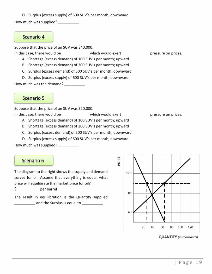
The diagram to the right shows the supply and demand
curves for oil. Assume that everything is equal, what
price will equilibrate the market price for oil?
$ __________ per barrel
The result in equilibration is the Quantity supplied
__________ and the Surplus is equal to __________
PR
ICE
120
80
40
20 40 60 80 100 120
QUANTITY (in thousands)
P a g e 2 0 |
Chapter 3 – Elasticity
The lessons on the importance of elasticity illustrate how it can have an effect on price and how price increases and decreases can have an impact on quantity demand and how it could effect a firm’s total revenue.
The price elasticity of demand measures the responsiveness of quantity demanded to a change in price. Price elasticity is defined as the percentage change in quantity demanded divided by the percentage change in price. To determine this price elasticity of demand (ED) = percentage change in quantity demanded percentage change in price.
ED = Percent Change in Quantity Demanded
Percent Change in Price
Note that, following the law of demand, price and quantity demanded show an inverse relationship. For this reason, the price elasticity of demand is, in theory, always negative. But in practice and for simplicity, this quantity is always expressed in absolute value terms—that is, as a positive number.
This chapter will contain a series of five working exercises with various scenarios to help reinforce the student’s understanding on how elasticity works. These exercises include the topics:
o Elastic Supply and Demand Curves
o Inelastic Supply and Demand Curves
o The Percent Changes of Price
o The Percent Changes in Quantity Demanded
o Elasticity Of Demand

| P a g e 2 1
This exercise is designed to help reinforce the student’s understanding of the topic of elasticity. This exercise can be used in conjunction with any economics textbook that addresses this topic.
NOTE: As you are working through each scenario in this exercise make sure that you label all parts of your diagrams to avoid mistakes. This exercise should be done using a ruler if necessary so that your lines are accurate and pencil and eraser so that you can make changes if you make a mistake. Do not use pen!
Refer to the illustration to the right. Which of the
graphs best illustrates an elastic demand curve? Circle
the letter of your choice.
A. Graph A
B. Graph B
C. Graph C
D. Graph D Graph A Graph B
PR
ICE
PR
ICE
P2
P1
P2 P1
Q2 Q1
QUANTITY Q2 Q1
QUANTITY
Graph C Graph D
PR
ICE
PR
ICE
P2
P1
P2
P1
Q2 Q1
QUANTITY
Q2=Q1 QUANTITY
Refer to the illustration to the right. Which of the
graphs best illustrates a perfectly elastic demand
curve? Circle the letter of your choice.
A. Graph A
B. Graph B
C. Graph C
D. Graph D
Graph A Graph B
PR
ICE
PR
ICE
P2
P1
P2 P1
Q2 Q1
QUANTITY Q2 Q1 QUANTITY
Graph C Graph D
PR
ICE
PR
ICE
P2
P1
P2
P1
Q2 Q1
QUANTITY
Q2=Q1 QUANTITY

P a g e 2 2 |
Refer to the illustration to the right. Which of the
graphs best illustrates a perfectly inelastic demand
curve? Circle the letter of your choice.
A. Graph A
B. Graph B
C. Graph C
D. Graph D
Graph A Graph B
PR
ICE
PR
ICE
P2
P1
P2 P1
Q2 Q1
QUANTITY Q2 Q1 QUANTITY
Graph C Graph D
PR
ICE
PR
ICE
P2
P1
P2
P1
Q2 Q1
QUANTITY Q2=Q1 QUANTITY
Using the Figure to the right, calculate the Total Revenue when a) the price is $9.00; b) the price is $8.00; c) the price is $2.00; and d) the price is $1.00. Use the space below to show your formulas and results.
PR
ICE
9
8
7
6
5
4
3
2
1
2 4 6 8 10 12 14 16 18
QUANTITY

| P a g e 2 3
This exercise is designed to help reinforce the student’s understanding of the topic of elasticity. This exercise can be used in conjunction with any economics textbook that addresses this topic.
NOTE: As you are working through each scenario in this exercise make sure that you label all parts of your diagrams to avoid mistakes. This exercise should be done using a ruler if necessary so that your lines are accurate and pencil and eraser so that you can make changes if you make a mistake. Do not use pen!
The illustration to the right shows the demand for a good. Use the information below and the illustration to the right to solve the following scenarios.
P4 = $15.00 Q1 = 3.0
P3 = 10.00 Q2 = 4.0
P2 = 6.00 Q3 = 6.0
P1 = 5.00 Q4 = 9.0 Table 1
Consider the points between X and Y. The price changes by __________ % The quantity demanded changes by __________ % The elasticity of demand is __________ This is considered to be __________
PRICE Demand
P4
P3
P2
P1
X
Y
Z
S
Q1 Q2 Q3 Q4 QUANTITY
Use the information from Table 1 and the illustration above to help solve this scenario. Consider the points between Y and Z. The price changes by approximately __________ % and the quantity demanded changes by approximately __________ %. In this region the demand is __________.
Use the information from Table 1 and the illustration above to help solve this scenario. Consider the points between Z and S. The price changes by approximately __________ % and the quantity demanded changes by approximately __________ %. In this region the elasticity of demand is __________ and is therefore considered to be __________.
P a g e 2 4 |
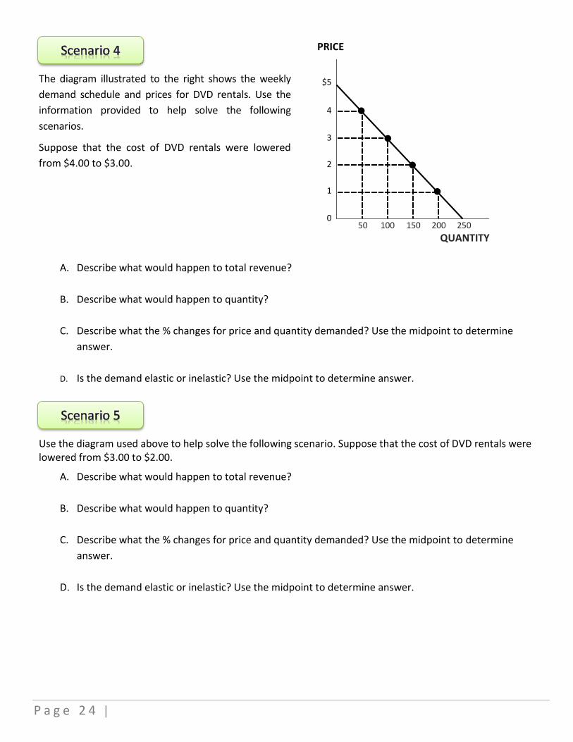
The diagram illustrated to the right shows the weekly
demand schedule and prices for DVD rentals. Use the
information provided to help solve the following
scenarios.
Suppose that the cost of DVD rentals were lowered
from $4.00 to $3.00.
PRICE
$5
4
3
2
1
0
50 100 150 200 250
QUANTITY
A. Describe what would happen to total revenue?
B. Describe what would happen to quantity?
C. Describe what the % changes for price and quantity demanded? Use the midpoint to determine
answer.
D. Is the demand elastic or inelastic? Use the midpoint to determine answer.
Use the diagram used above to help solve the following scenario. Suppose that the cost of DVD rentals were lowered from $3.00 to $2.00.
A. Describe what would happen to total revenue?
B. Describe what would happen to quantity?
C. Describe what the % changes for price and quantity demanded? Use the midpoint to determine
answer.
D. Is the demand elastic or inelastic? Use the midpoint to determine answer.

| P a g e 2 5
This exercise is designed to help reinforce the student’s understanding of the topic of elasticity. This exercise can be used in conjunction with any economics textbook that addresses this topic.
NOTE: As you are working through each scenario in this exercise make sure that you label all parts of your diagrams to avoid mistakes. This exercise should be done using a ruler if necessary so that your lines are accurate and pencil and eraser so that you can make changes if you make a mistake. Do not use pen!
Using a Slope equal to -1;
1. Calculate the % change in price. 2. Calculate the % change in quantity. 3. Calculate the % elasticity of
demand. 4. Show the translations of different
values of elasticity. 5. Plot the elasticity numbers.
Note the elasticity numbers as you move down the demand curve and show where it is Perfectly Elastic and Perfectly Inelastic.
PR
ICE
9
8
7
6
5
4
3
2
1
1 2 3 4 5 6 7 8 9 QUANTITY
P Q %P %Q ED
10 9 0 1 _____% _____% _____
9 8 1 2 _____% _____% _____

P a g e 2 6 |
This exercise is designed to help reinforce the student’s understanding of the topic of elasticity as it effects revenue. This exercise can be used in conjunction with any economics textbook that addresses this topic.
NOTE: As you are working through each scenario in this exercise make sure that you label all parts of your diagrams to avoid mistakes. This exercise should be done using a ruler if necessary so that your lines are accurate and pencil and eraser so that you can make changes if you make a mistake. Do not use pen!
For most supply and demand curves price elasticity along a curve varies. With most goods we can refer to any particular point or section of a demand or supply curve. At each various point along the curve your elasticity varies. Use the figure to the right to show how elasticity varies along the linear curve by graphing elasticity and graphing the total revenues as it relates to the curve.
1. Where are the elastic points of the Demand Curve? Show this on your graph.
2. Where are the inelastic points of the Demand Curve? Show this on your graph.
3. At what point is it unit elastic? Show this on your graph. NOTE: Keep in mind Elastic: ED>1, Inelastic: ED<1, Unit Elastic: ED=1.
What happens to ED if the price changes from $16 to $18? Change from $4 to $6?
PR
ICE
(s)
$18
2
2 4 6 8 10 12 14 16 18 QUANTITY
TOTA
L R
EVEN
UE
(s)
$90
50
10
2 4 6 8 10 12 14 16 18 QUANTITY
$36
$84

| P a g e 2 7
This exercise is designed to help reinforce the student’s understanding of the topic of elasticity. This exercise can be used in conjunction with any economics textbook that addresses this topic.
NOTE: As you are working through each scenario in this exercise make sure that you label all parts of your diagrams to avoid mistakes. This exercise should be done using a ruler if necessary so that your lines are accurate and pencil and eraser so that you can make changes if you make a mistake. Do not use pen!
1. Use the illustration to the right to determine the following:
A. What is the % change when the price decreases from
$25.00 to $15.00? ___________
B. What is the % change for quantity when the price
decreases from $25.00 to $15.00? ____________
C. What is ED when the price decreases?
___________
D. What is the Total Revenue? ____________
E. Is demand Elastic or Inelastic? ___________
F. What is the % change for price when the price increases
from $15 to $25? ____________
G. What is the % change for quantity when the price
increases from $15 to $25? ____________
H. What is ED when the price increases? ____________
I. What is Total Revenue? ____________
J. Is demand Elastic or Inelastic? ___________
Formula using the Midpoint:
ED = Percent Change in Quantity Demanded
Percent Change in Price
= QD / Q AVE
P / P AVE
PR
ICE
$25
15
B
A
D
20 40 60
QUANTITY (in millions)
2. Determine the following using the midpoint formula from above?
A. What is the ED? _________________
B. Is demand Elastic or Inelastic? ________________
3. What determination would you make based on your findings?
P= P AVE
Q AVE
ED = ___ at midpoint between point A and B.
QD=

P a g e 2 8 |
Externalities are common in virtually every area of economic activity. They are defined spill-over effects arising from the production and/or consumption of goods and services for which no appropriate compensation is paid. Externalities can cause market failure if the price mechanism does not take into account the full social costs and social benefits of production and consumption.
This chapter will contain a working exercises with various scenarios to help reinforce the student’s understanding of externalities and its effects. These exercises include the topics:
o Private Costs
o Social Costs
o Market Equilibrium
o Efficient Equilibrium
| P a g e 2 9
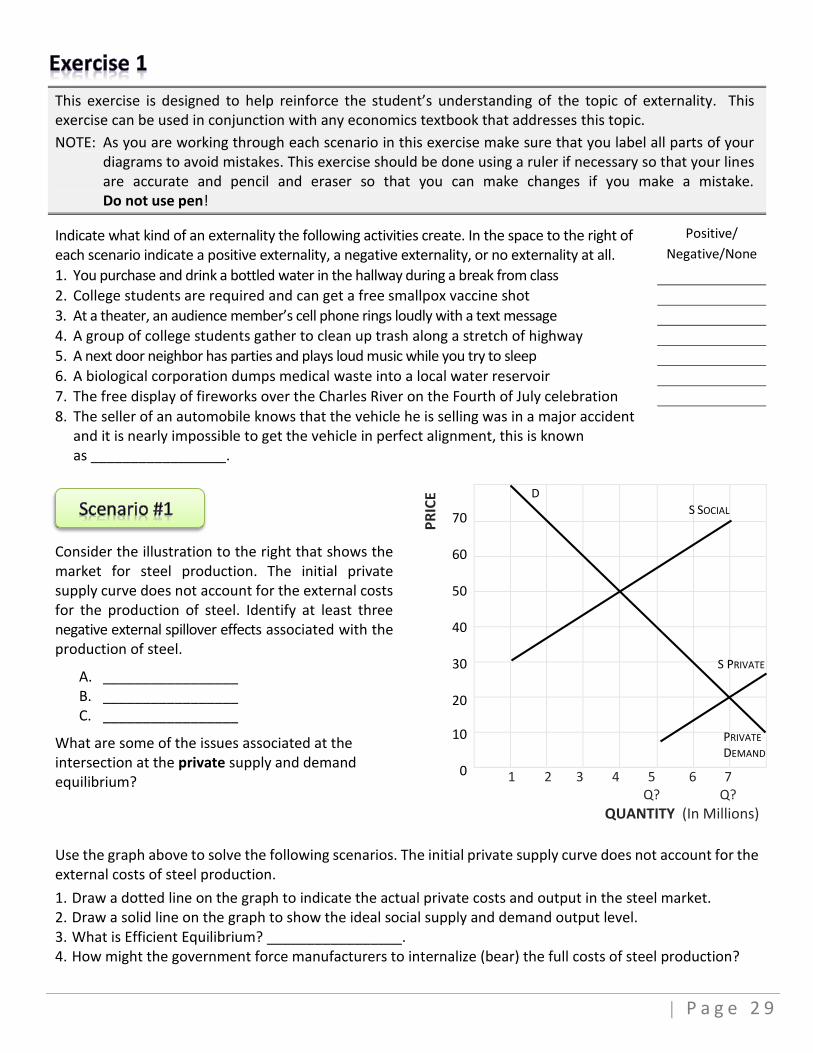
This exercise is designed to help reinforce the student’s understanding of the topic of externality. This exercise can be used in conjunction with any economics textbook that addresses this topic.
NOTE: As you are working through each scenario in this exercise make sure that you label all parts of your diagrams to avoid mistakes. This exercise should be done using a ruler if necessary so that your lines are accurate and pencil and eraser so that you can make changes if you make a mistake. Do not use pen!
Indicate what kind of an externality the following activities create. In the space to the right of each scenario indicate a positive externality, a negative externality, or no externality at all.
Positive/
Negative/None
1. You purchase and drink a bottled water in the hallway during a break from class
2. College students are required and can get a free smallpox vaccine shot
3. At a theater, an audience member’s cell phone rings loudly with a text message
4. A group of college students gather to clean up trash along a stretch of highway
5. A next door neighbor has parties and plays loud music while you try to sleep
6. A biological corporation dumps medical waste into a local water reservoir
7. The free display of fireworks over the Charles River on the Fourth of July celebration
8. The seller of an automobile knows that the vehicle he is selling was in a major accident and it is nearly impossible to get the vehicle in perfect alignment, this is known as _________________.
Consider the illustration to the right that shows the market for steel production. The initial private supply curve does not account for the external costs for the production of steel. Identify at least three negative external spillover effects associated with the production of steel.
A. _________________ B. _________________ C. _________________
What are some of the issues associated at the intersection at the private supply and demand equilibrium?
PR
ICE
70
60
50
40
30
20
10
0
D
1 2 3 4 5 6 7 Q? Q?
QUANTITY (In Millions)
Use the graph above to solve the following scenarios. The initial private supply curve does not account for the external costs of steel production.
1. Draw a dotted line on the graph to indicate the actual private costs and output in the steel market. 2. Draw a solid line on the graph to show the ideal social supply and demand output level. 3. What is Efficient Equilibrium? _________________. 4. How might the government force manufacturers to internalize (bear) the full costs of steel production?
S PRIVATE
S SOCIAL
PRIVATE
DEMAND
P a g e 3 0 |
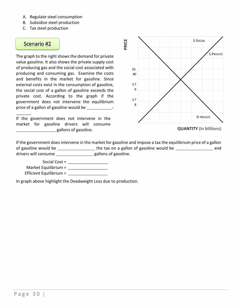
A. Regulate steel consumption B. Subsidize steel production C. Tax steel production
The graph to the right shows the demand for private value gasoline. It also shows the private supply cost of producing gas and the social cost associated with producing and consuming gas. Examine the costs and benefits in the market for gasoline. Since external costs exist in the consumption of gasoline, the social cost of a gallon of gasoline exceeds the private cost. According to the graph if the government does not intervene the equilibrium price of a gallon of gasoline would be ___________-
______. If the government does not intervene in the market for gasoline drivers will consume _________________ gallons of gasoline.
PR
ICE
$3.
80
3.7
9
3.7
8
QUANTITY (In Millions)
If the government does intervene in the market for gasoline and impose a tax the equilibrium price of a gallon of gasoline would be ________________ the tax on a gallon of gasoline would be ________________ and drivers will consume ________________ gallons of gasoline.
Social Cost = _________________ Market Equilibrium = _________________ Efficient Equilibrium = _________________
In graph above highlight the Deadweight Loss due to production.
S SOCIAL
D PRIVATE
S PRIVATE

| P a g e 3 1
The government can sometimes improve economic well-being by remedying externalities through pollution taxes, regulation and subsidies, and providing public goods.
In this chapter, we will see how the government obtains revenues through taxation to provide these goods and services. We also examine the different types of taxation. The last section of the chapter is on public choice economics, the application of economic principles to politics.
This chapter will contain exercises with various scenarios to help reinforce the student’s understanding of some of the various ways government generate revenue to provide goods and services to the public, and a cap and trade system for controlling externalities using a regulation approach. These exercises include the topics:
o Flat Tax System
o Cap and Trade

P a g e 3 2 |
This exercise is designed to help reinforce the student’s understanding the way government could collect taxes using a flat tax collection system. This exercise can be used in conjunction with any economics textbook that addresses this topic.
NOTE: This exercise should be done using pencil and eraser so that you can make changes if you make a mistake. Do not use pen!
Consider the following Flat Tax problem. Suppose a flat tax plan would allow all individuals to deduct a standard allowance of $25,000 from their wages. If the flat tax rate was 15% and the individual made a salary of $27,660.00 what would be the Marginal Tax Rate percentage after the stipulated standard allowance? How much taxes would be paid on a salary of $37,660?
Answer: _________________%
$________________
Use the space to the right to solve your problem. What are some of the issues opponents feel of a flat tax versus our current tax system?
A. ________________________________ B. ________________________________
________________________________
Consider the following Flat Tax problem. Suppose a flat tax plan would allow all individuals to deduct a standard allowance of $20,000 from their wages. If the flat tax rate was 15% and the individual made a salary of $125,600, what would be the Marginal Tax Rate percentage after the stipulated standard allowance? How much taxes would be paid on a salary of $125,600?
Answer: _________________%
$________________

| P a g e 3 3
Consider the following Flat Tax problem. Suppose a flat tax plan would allow all individuals to deduct a standard allowance of $20,000 from their wages. If the flat tax rate was 15% and the individual made a salary of $61,000, what would be the Marginal Tax Rate percentage after the stipulated standard allowance? How much taxes would be paid on a salary of $61,000?
Answer: _________________%
$________________
Consider the following Flat Tax problem. Suppose a flat tax plan would allow all individuals to deduct a standard allowance of $25,000 from their wages. If the flat tax rate was 15% and the individual made a salary of $1,000,000, what would be the Marginal Tax Rate percentage after the stipulated standard allowance? How much taxes would be paid on a salary of $1,000,000?
Answer: _________________%
$________________
In your opinion who would benefit from a flat tax system? Why?

P a g e 3 4 |
This exercise is designed to help reinforce the student’s understanding of the topic of Cap and Trade that could be used by government to help regulate and control pollution. This exercise can be used in conjunction with any economics textbook that addresses this topic.
NOTE: As you are working through each scenario in this exercise make sure that you complete all parts of each scenario so that you can contrast and compare that three options being covered. This exercise should be done using pencil and eraser so that you can make changes if you make a mistake.
Do not use pen!
Cap and Trade: Option 1
The government’s goal would be to reduce pollution by 120 units. With this option the government gives each firm 40 non-tradable permits. The burden is then on each firm to reduce pollution to meet the government goal. Use the information to the right to determine what is the total cost to reduce pollution?
NOTE: Economists are only concerned about efficiency. Based on your findings are there any incentives for firms to reduce pollution with this option?
Firm Initial Pollution Cost/Unit to Reduce
A 70 Units $20
B 80 Units $25
C 50 Units $10
Firm Need to Reduce Cost to Reduce
A
B
C
Total system cleanup cost = $
Cap and Trade: Option 2
In this option the government’s goal would again be to reduce pollution by 120 units. In this option the government would give each firm 40 tradable permits. Think about what each firm has to do to comply with the government restrictions. Because each firm could trade their permits, complete what you think the market outcomes would be in the table to the right.
Firm Initial Pollution Cost/Unit to Reduce
A 70 Units $20
B 80 Units $25
C 50 Units $10
Firm Market Outcomes
A
B
C

| P a g e 3 5
Using the tables to the right determine who you think is going to buy and who is going to sell rather than reduce pollution?
Permit Who is willing to buy; how many?
Price < $10
Price < $20
Price < $25
Price > $25
Permit Who is willing to sell; how many?
Price < $10
Price < $20
Price < $25
Price > $25
Cap and Trade: Option 3 In this option the government’s goal again is to reduce pollution by 120 units! In this option the government will auction off 120 permits, running what’s known as a 2nd price auction. That means the firm with highest bid pays the amount of the second highest bid. Using the tables to the right, determine how each company would bid on permits to determine the best way to reduce pollution.
Firm Initial Pollution Cost/Unit to Reduce
A 70 Units $20
B 80 Units $25
C 50 Units $10
Firm Auction Prices
A
B
C
In the table below complete how you think each firm would react to this government option and determine what the total cleanup costs to the system would be.
Firm Permit Cost Cleanup Costs Total Costs
A
B
C
Total system cleanup cost = $

P a g e 3 6 |
In this chapter, we focus on how consumers allocate their income between various combinations of goods. This decision involves trade-offs because if you buy more of one good, you may not be able to afford as much of another good. How do consumers choose certain combinations of goods with their fixed available budget desires and fulfill desires for more than one combinations of goods? We address these questions in this chapter to strengthen our understanding of the law of demand.
This chapter will contain exercises with various scenarios to help reinforce the student’s understanding of some of the various ways consumer choices are made. These exercises include the topics:
o Total Utility
o Marginal Utility

| P a g e 3 7
This exercise is designed to help reinforce the student’s understanding of the topic of consumer choice based on total and marginal utility. This exercise can be used in conjunction with any economics textbook that addresses this topic.
NOTE: As you are working through this exercise make sure that you label all parts of your diagrams to avoid mistakes. This exercise should be done using a ruler so that your lines are accurate and pencil and eraser so that you can make changes if you make a mistake. Do not use pen!
Steven plays a lot of basketball with his friends.
Table 1 to the right contains information on Steven's
utility from eating energy bars while playing
basketball with his friends.
Energy Bars Total Utility (Utils)
0 0
1 12
2 22
3 30
4 36
5 40
6 42
Table 1
Using the graph to the right and the information in
Table 1 plot Steven’s total utility (TU) curve for
eating his first six energy bars while playing
basketball on the graph to the right. Plot the line
segments to connect the points. Remember to plot
from left to right.
48
42
36
30
24
18
12
6
Tota
l Uti
lity
(U
tils
)
1 2 3 4 5 6 7
Energy Bars Eaten

P a g e 3 8 |
Using the graph to the right and the information in
Table 1 plot Steven's marginal utility (MU) curve
from eating his first six energy bars while playing
basketball. Plot the line segments to connect the
points. Remember to plot from left to right and to
plot between integers.
For Steven increasing the eating of energy bars
results in __________ marginal utility.
16
14
12
10
8
6
4
2
Mar
gin
al U
tilit
y (
Uti
ls)
1 2 3 4 5 6 7
Energy Bars Eaten

| P a g e 3 9
This exercise is designed to help reinforce the student’s understanding of the topic of consumer choice based on total and marginal utility. This exercise can be used in conjunction with any economics textbook that addresses this topic.
NOTE: As you are working through this exercise make sure that you label all parts of your diagrams to avoid mistakes. This exercise should be done using a ruler so that your lines are accurate and pencil and eraser so that you can make changes if you make a mistake. Do not use pen!
Ralph enjoys drinking milk because it will make him
grow up to be big and strong. Table 1 to the right
contains the utility from drinking milk. Fill-in the
missing utils.
Milk
(Glasses/Day)
Total Utility
(Utils/Day)
Marginal Utility
(Utils/Glass)
0 0
1 18 18
2 15
3 45 12
4 54
5 60 6
6 63 3
7 60
Table 1
Using the graph to the right, plot Ralphs Total Utility
curve if he consumes 0, 1, 2, 3, 4, 5, 6, or 7 glasses of
milk per day.
64
56
48
40
32
24
16
8
Tota
l Uti
lity
(U
tils
)
1 2 3 4 5 6 7 Energy Bars Eaten
P a g e 4 0 |
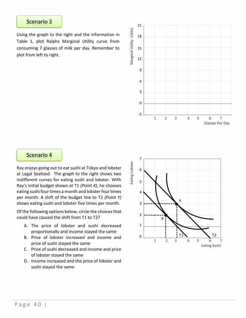
Using the graph to the right and the information in
Table 1, plot Ralphs Marginal Utility curve from
consuming 7 glasses of milk per day. Remember to
plot from left to right.
21
18
15
12
9
6
3
0
-3
Mar
gin
al U
tilit
y (
Uti
ls)
1 2 3 4 5 6 7 Glasses Per Day
Ray enjoys going out to eat sushi at Tokyo and lobster at Legal Seafood. The graph to the right shows two indifferent curves for eating sushi and lobster. With Ray’s initial budget shown at T1 (Point X), he chooses eating sushi four times a month and lobster four times per month. A shift of the budget line to T2 (Point Y) shows eating sushi and lobster five times per month.
Of the following options below, circle the choices that could have caused the shift from T1 to T2?
A. The price of lobster and sushi decreased proportionally and income stayed the same
B. Price of lobster increased and income and price of sushi stayed the same
C. Price of sushi decreased and income and price of lobster stayed the same
D. Income increased and the price of lobster and sushi stayed the same
7
6
5
4
3
2
1
0
Eati
ng
Lob
ster
Y
X
T1
T2
1 2 3 4 5 6 7 Eating Sushi

| P a g e 4 1
This exercise is designed to help reinforce the student’s understanding of the topic of consumer choice based on marginal utility. This exercise can be used in conjunction with any economics textbook that addresses this topic.
NOTE: As you are working through this exercise make sure that you total all parts of your diagrams to avoid mistakes. Do not use pen!
Ralph is faced with having to make a decision of choosing between mini pizzas and smoothies. They are priced at $2.00 for mini pizzas and $1.00 for smoothies. The marginal utility derived from each of the two good is outlined in Table 1 and Table 2.
Ralph’s lunch budget for each week is $11.00.
If Ralph had no budget constraints, what would be the maximum marginal utility he could receive by consuming both products?
How much would that cost him?
Ralph however as you know does have a budget. With that in mind’ what is the best way for him to spend his budget and get the best bang for the buck of mini pizzas and smoothie purchases?
Use the following formula to determine how Ralph should spend his money.
MUMP/PMP = MUS/PS
NOTE: Remember economic decisions are made at the marginal level.
Marginal Utility
from the last
Mini Pizza (MP)
Quantity of
Mini Pizza’s (MP)
consumed/week
MUMP/PMP
20 1 10
16 2 8
14 3 7
10 4 5
8 5 4
Table 1
Marginal Utility
from the last
Smoothie
Quantity of
Smoothies
consumed/week
MUS/PS
12 1 12
10 2 10
5 3 6
4 4 4
3 5 3
Table 2

P a g e 4 2 |
Production and costs refers to the output of goods and services produced by businesses within a market. This production creates the supply that allows our needs and wants to be satisfied. To simplify the idea of the production function, economists create a number of time periods for analysis. Topics generally concentrated on when dealing with production and costs are marginal revenue and marginal profit.
Marginal revenue is the increase in revenue that results from the sale of one additional unit of output. Marginal revenue is calculated by dividing the change in total revenue by the change in output quantity. While marginal revenue can remain constant over a certain level of output, it follows the law of diminishing returns and will eventually slow down, as the output level increases.
Marginal profit is the term used to refer to the difference between the marginal cost and the marginal revenue for producing one additional unit of production.
This chapter will contain exercises with various scenarios to help reinforce the student’s understanding of the key topics of production and costs and how it would affect revenue and profit. These exercises include the topics:
o Marginal Revenue
o Marginal Costs
o Total Revenue
o Profit

| P a g e 4 3
Exercise 1 This exercise is designed to help reinforce the student’s understanding of the topic of fixed costs, variable costs, implicit costs, and explicit costs. This exercise can be used in conjunction with any economics textbook that addresses this topic.
NOTE: Fill-in the answer for each of the following questions in the spaces provided. This exercise should be done using a pencil and eraser so that you can make changes if you make a mistake.
Do not use pen!
1. Profits are defined as __________ minus __________.
2. The cost of producing a good is measured by the worth of the __________ alternative that was
given up to obtain the resource.
3. Explicit costs are input costs that require a(n) __________ payment.
4. Whenever we talk about cost—explicit or implicit—we are talking about __________ cost.
5. Economists generally assume that the ultimate goal of a firm is to __________ profits.
6. Accounting profits equal actual revenues minus actual expenditures of cash explicit costs, so
they do not include __________ costs.
7. Economists consider a zero economic profit a normal profit because it means that the firm is
covering both __________ and __________ costs—the total opportunity cost of its resources.
8. __________ are costs that have already been incurred and cannot be recovered.
9. Because it takes more time to vary some inputs than others, we must distinguish between
the __________ run and the __________ run.
10. The long run is a period of time in which the firm can adjust __________ inputs.
P a g e 4 4 |
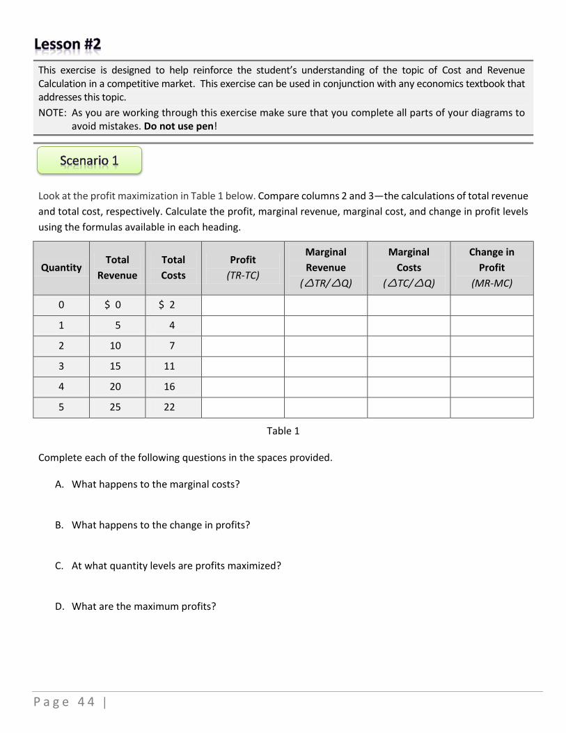
This exercise is designed to help reinforce the student’s understanding of the topic of Cost and Revenue Calculation in a competitive market. This exercise can be used in conjunction with any economics textbook that addresses this topic.
NOTE: As you are working through this exercise make sure that you complete all parts of your diagrams to avoid mistakes. Do not use pen!
Look at the profit maximization in Table 1 below. Compare columns 2 and 3—the calculations of total revenue
and total cost, respectively. Calculate the profit, marginal revenue, marginal cost, and change in profit levels
using the formulas available in each heading.
Quantity Total
Revenue
Total
Costs
Profit
(TR-TC)
Marginal
Revenue
(TR/Q)
Marginal
Costs
(TC/Q)
Change in
Profit
(MR-MC)
0 $ 0 $ 2
1 5 4
2 10 7
3 15 11
4 20 16
5 25 22
Table 1
Complete each of the following questions in the spaces provided.
A. What happens to the marginal costs?
B. What happens to the change in profits?
C. At what quantity levels are profits maximized?
D. What are the maximum profits?
| P a g e 4 5
Use the graph to the right and the information established
in Table 1 above to plot Marginal Revenue, Marginal Costs,
Profit, and Change in Profit.
A. Based on your findings in Table 1 and your graph to
the right, what would the best plan for production
be?
Co
sts
Quantity of Output