Introduction to Mathematical ProgrammingIE406

Lecture 9

Dr. Ted Ralphs

IE406 Lecture 9 1

Reading for This Lecture

• AMPL Book: Chapter 1

• AMPL: A Mathematical Programming Language

• GMPL User’s Guide

• ZIMPL User’s Guide

1

IE406 Lecture 9 2

Software for Mathematical Programs

• So far, we have seen how to solve linear programs by hand.

• In practice, most people use third-party software.

• Most solvers have the simplex method and some others.

• Commercial solvers

– CPLEX ← available in ISE– XPRESS-MP ← available in ISE– MOSEK– LINDO

• Open source solvers (free to download and use)

– CLP– DYLP– GLPK– SOPLEX– lp solve– SYMPHONY

2

IE406 Lecture 9 3

File Formats for Mathematical Programs

• Question: How do we tell the solver what the linear program is?

• One possible approach:

– Formulate the model.– Generate the constraint matrix for your instance and data.– Export the entire constraint matrix to a file using a standard format.– Pass the file to a solver.– Get the answer and interpret it in terms of the original model.

• File formats for mathematical programs

– MPS– LP– LPFML

• Problems with this approach:

– The constraint matrices can be huge.– It is tedious to generate them.– You can’t easily modify the model parameters or data.– Different solvers accept different file formats.

3

IE406 Lecture 9 4

Modeling Languages

• Modeling languages provide an interface between the user and the solver.

• They allow the user to

– input the model in a “natural” format.

– easily modify parameters and data.

– work with multiple solvers.

• Commercial modeling languages

– GAMS– LINGO– MPL– AMPL ← available in ISE– LINGO– MOSEL– OPL ← available in ISE

• Open source modeling languages (free to download and use)

– GMPL– ZIMPL

4

IE406 Lecture 9 5

AMPL

• Currently, the most commonly used modeling language is probablyAMPL, but many other languages are similar in concept.

• AMPL has many of the features of a programming language, includingloops and conditionals.

• Most available solvers will read AMPL models.

• GMPL and ZIMPL are open source languages that implements subsetsof AMPL.

• AMPL models can be read by CPLEX, which is one of the commercialsolver available in the ISE department.

• You can also submit AMPL models to the NEOS server.

• Student versions can be downloaded from www.ampl.com.

5

IE406 Lecture 9 6

Other Options

• ZIMPL

– ZIMPL is a stand-alone executable that translates models written in aformat similar to AMPL into MPS format, which can be read by mostsolvers.

– A ZIMPL executable can be downloaded from www.zib.de/koch/zimpl

• OPL

– OPL Studio is a modeling IDE available in the ISE department.– The model format is similar to AMPL.

• GMPL

– Another language very similar to AMPL.– Works with GLPK, CLP, and SYMPHONY.

6

IE406 Lecture 9 7

AMPL Concepts

• In many ways, AMPL is like any other programming language.

• Example: A simple product mix problem.

ampl: option solver cplex;ampl: var X1;ampl: var X2;ampl: maximize profit: 3*X1 + 3*X2;ampl: subject to hours: 3*X1 + 4*X2 <= 120000;ampl: subject to cash: 3*X1 + 2*X2 <= 90000;ampl: subject to X1_limit: X1 >= 0;ampl: subject to X2_limit: X2 >= 0;ampl: solve;CPLEX 7.1.0: optimal solution; objective 1050002 simplex iterations (0 in phase I)ampl: display X1;X1 = 20000ampl: display X2;X2 = 15000

7

IE406 Lecture 9 8

Storing Commands in a File

• You can type the commands into a file and then load them.

• This makes it easy to modify your model later.

• Example:

ampl: option solver cplex;ampl: model simple.mod;ampl: solve;CPLEX 7.1.0: optimal solution; objective 1050002 simplex iterations (0 in phase I)ampl: display X1;X1 = 20000ampl: display X2;X2 = 15000

8

IE406 Lecture 9 9

Generalizing the Model

• Suppose we want to generalize this production model to more than twoproducts.

• AMPL allows the model to be separated from the data.

• Components of a linear program in AMPL

– Data

∗ Sets: lists of products, raw materials, etc.∗ Parameters: numerical inputs such as costs, production rates, etc.

– Model

∗ Variables: Values in the model that need to be decided upon.∗ Objective Function: A function of the variable values to be

maximized or minimized.∗ Constraints: Functions of the variable values that must lie within

given bounds.

9

IE406 Lecture 9 10

Example: Production Model

set prd; # products

param price {prd}; # selling priceparam cost {prd}; # cost per unit for raw materialparam hours {prd}; # hours of machine to produceparam max_cash; # total cash availableparam max_prd; # total production hours available

var make {prd} >= 0; # number of units to manufacture

maximize profit: sum{i in prd} (price[i]-cost[i])*make[i];

subject to hours: sum{i in prd} hours[i]*make[i] <= max_prd;

subject to cash: sum{i in prd} cost[i]*make[i] <= max_cash;

10

IE406 Lecture 9 11

Example: Production Model Data

set prd := widgets gadgets;

param max_prd := 120000;param max_cash := 90000;

param: price cost hours :=widgets 6 3 3gadgets 5 2 4;

11

IE406 Lecture 9 12

Solving the Production Model

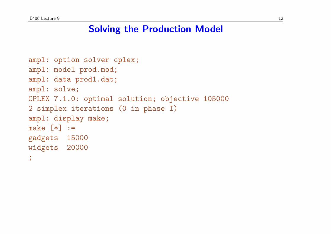
ampl: option solver cplex;ampl: model prod.mod;ampl: data prod1.dat;ampl: solve;CPLEX 7.1.0: optimal solution; objective 1050002 simplex iterations (0 in phase I)ampl: display make;make [*] :=gadgets 15000widgets 20000;

12

IE406 Lecture 9 13

Changing the Parameters

• Suppose we want to increase available production hours by 2000.

• To resolve from scratch, simply modify the data file and reload.

ampl: reset data;ampl: data prod1.dat;ampl: solve;CPLEX 7.1.0: optimal solution; objective 1060002 simplex iterations (0 in phase I)ampl: display make;make [*] :=gadgets 16000widgets 19333.3;

13

IE406 Lecture 9 14

Retaining the Current Basis

• Instead of resetting all the data, you can modify one element.

ampl: reset data max_prd;ampl: data;ampl data: param max_prd := 122000;ampl data: solve;CPLEX 7.1.0: optimal solution; objective 1060000 simplex iterations (0 in phase I)ampl: display make;make [*] :=gadgets 16000widgets 19333.3;

• Notice that the basis was retained.

14

IE406 Lecture 9 15

Extending the Model

• Now suppose we want to add another product.

set prd := widgets gadgets watchamacallits;

param max_prd := 120000;param max_cash := 90000;

param: price cost hours :=widgets 6 3 3gadgets 5 2 4

watchamacallits 4 1 3;

15

IE406 Lecture 9 16

Solving the Extended Model

ampl: reset data;ampl: data prod2.dat;ampl: solve;CPLEX 7.1.0: optimal solution; objective 1200002 simplex iterations (0 in phase I)ampl: display make;make [*] :=

gadgets 0watchamacallits 15000

widgets 25000;

16

IE406 Lecture 9 17

Indexing Constraints

Now we’re going to add multiple machine types.

set prd; # productsset mach; # machine typesparam price {prd}; # selling priceparam cost {prd}; # cost of raw materialsparam hours {prd, mach}; # hours by product and machine typeparam max_cash; # total cash availableparam max_prd {mach}; # total production hours by machinevar make {prd} >= 0; # number of units to manufacture

maximize profit : sum {i in prd} (price[i] - cost[i]) * make[i];

subject to hours_limit {j in mach} :sum {i in prd} hours[i,j]*make[i] <= max_prd[j];

subject to cash_limit :sum {i in prd} cost[i]*make[i] <= max_cash;

17

IE406 Lecture 9 18

Solving the New Model

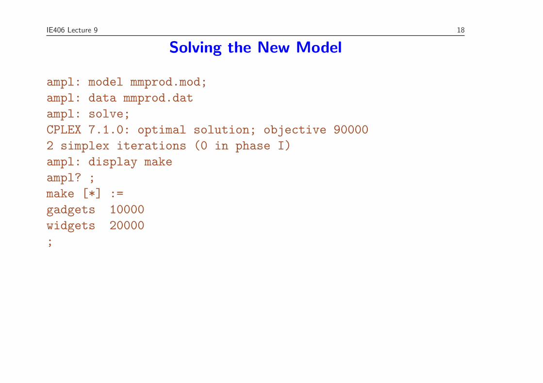
ampl: model mmprod.mod;ampl: data mmprod.datampl: solve;CPLEX 7.1.0: optimal solution; objective 900002 simplex iterations (0 in phase I)ampl: display makeampl? ;make [*] :=gadgets 10000widgets 20000;

18

IE406 Lecture 9 19

Callable Libraries

• More sophisticated users may prefer to access the solver directly fromapplication code without going through a modeling language.

• Each solver has its own API for doing this.

• With this approach, the user is forced to work with a particular solver.

• Solution: The Open Solver Interface (OSI).

19

IE406 Lecture 9 20

Computational Infrastructure for Operations Research(COIN-OR)

• The COIN-OR Foundation is a consortium of researchers from bothindustry and academia.

• COIN-OR is dedicated to promoting the development and use ofinteroperable, open-source software for operations research.

• We are also dedicated to defining standards and interfaces that allowsoftware components to interoperate with other software, as well as withusers.

• Check out the Web site for the project at

http://www.coin-or.org

20

IE406 Lecture 9 21

The Open Solver Interface

• The Open Solver Interface (OSI) is a uniform API available from COIN-OR that provides a common interface to numerous solvers.

• Using the OSI improves portability and eliminates dependence on third-party software.

• There is a tutorial that explains the basics of using the OSI at

http://coral.ie.lehigh.edu/~coin

21

IE406 Lecture 9 22

C++ Modeling Objects

• FlopC++ is an open source library of C++ modeling objects that canbe used to generate models directly in C++.

• FlopC++ will work with any solver that has an OSI interface.

• ILOG’s Concert Technology is another library for building models directlyin C++.

• A new version of OSI due out soon will also include C++ modelingobjects.

22

IE406 Lecture 9 23

Spreadsheet optimization

• For quick and dirty modeling, Excel provides a built-in interpreter forbuilding mathematical programming models.

• The built-in solver is not very robust, but can be upgraded.

• Spreadsheet modeling has significant limitations and is probably not themethod of choice.

23