introduction to machine learning - uni stuttgart · 2017-07-18 · introduction to machine learning...
TRANSCRIPT
Introduction to Machine Learning
Marc Toussaint / Duy Nguyen-Tuong
July 18, 2017
This is a direct concatenation and reformatting of all lecture slides from the MachineLearning course (summer term 2017, U Stuttgart) to help prepare for exams.
Contents
1 Introduction 3
2 Regression 11
3 Classification - Part 1 22
4 Classification - Part 2 30
5 Unsupervised Learning - Part 1 36
6 Unsupervised Learning - Part 2 42
7 The Breadth of MLNeural Networks & Deep Learning 48
1
2 Introduction to Machine Learning, Marc Toussaint
8 The Breadth of MLLocal Models & Boosting 57
9 The Breadth of MLCRF & Recap: Probability 70
10 Bayesian Regression & Classification 93
11 Graphical Models 102
Introduction to Machine Learning, Marc Toussaint 3
1 Introduction
What is Machine Learning?
1) A long list of methods/algorithms for different data anlysis problems– in sciences
– in commerce
2) Frameworks to develop your own learning algorithm/method
3) Machine Learning = information theory/statistics + computer science1:1
What is Machine Learning?
• Pedro Domingos: A Few Useful Things to Know about Machine LearningLEARNING = REPRESENTATION + EVALUATION + OPTIMIZATION
• “Representation”: Choice of model, choice of hypothesis space• “Evaluation”: Choice of objective function, optimality principle
Notes: The prior is both, a choice of representation and, usually, a part of theobjective function.In Bayesian settings, the choice of model often directly implies also the “objec-tive function”• “Optimization”: The algorithm to compute/approximate the best model
1:2
Pedro Domingos: A Few Useful Things to Know about Machine Learning• It’s generalization that counts
– Data alone is not enough
– Overfitting has many faces
– Intuition fails in high dimensions
– Theoretical guarantees are not what they seem
• Feature engineering is the key• More data beats a cleverer algorithm• Learn many models, not just one• Simplicity does not imply accuracy• Representable does not imply learnable• Correlation does not imply causation
4 Introduction to Machine Learning, Marc Toussaint
1:3
Machine Learning is everywhere
NSA, Amazon, Google, Zalando, Trading, Bosch, ...Chemistry, Biology, Physics, ...Control, Operations Research, Scheduling, ...
• Machine Learning ∼ Information Processing (e.g. Bayesian ML)1:4
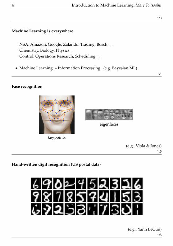
Face recognition
keypoints
eigenfaces
(e.g., Viola & Jones)1:5
Hand-written digit recognition (US postal data)
(e.g., Yann LeCun)1:6

Introduction to Machine Learning, Marc Toussaint 5
Autonomous Driving
1:7
Speech recognition
Siri
Echo with Alexa
1:8
Particle Physics

6 Introduction to Machine Learning, Marc Toussaint
(Higgs Boson Machine Learning Challenge)
1:9
Machine Learning became an important technologyin science as well as commerce
1:10
Examples of ML for behavior...
1:11
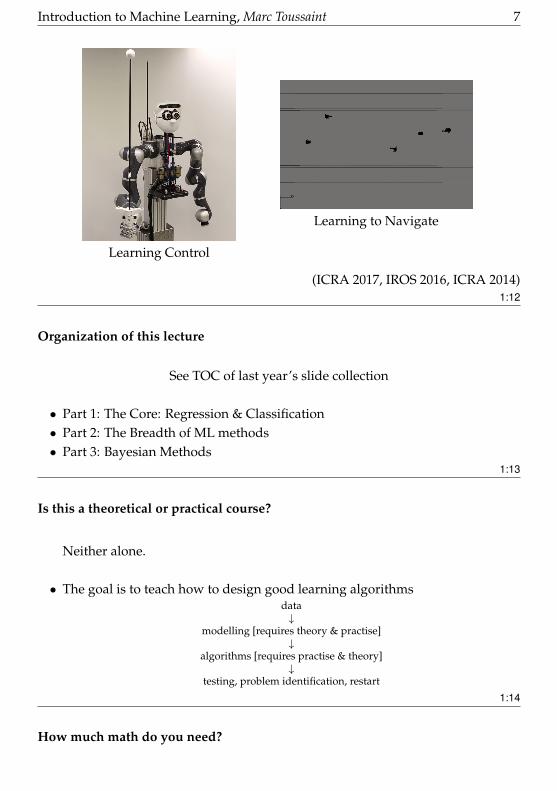
Robot Learning
Introduction to Machine Learning, Marc Toussaint 7
Learning Control
Learning to Navigate
(ICRA 2017, IROS 2016, ICRA 2014)1:12
Organization of this lecture
See TOC of last year’s slide collection
• Part 1: The Core: Regression & Classification• Part 2: The Breadth of ML methods• Part 3: Bayesian Methods
1:13
Is this a theoretical or practical course?
Neither alone.
• The goal is to teach how to design good learning algorithmsdata↓
modelling [requires theory & practise]↓
algorithms [requires practise & theory]↓
testing, problem identification, restart
1:14
How much math do you need?
8 Introduction to Machine Learning, Marc Toussaint
• Let L(x) = ||y −Ax||2. What is
argminx
L(x)
• Findminx||y −Ax||2 s.t. xi ≤ 1
• Given a discriminative function f(x, y) we define
p(y |x) =ef(y,x)∑y′ e
f(y′,x)
• Let A be the covariance matrix of a Gaussian. What does the Singular ValueDecomposition A = V DV> tell us?
1:15
How much coding do you need?
• A core subject of this lecture: learning to go from principles (math) to code
• Many exercises will implement algorithms we derived in the lecture and collectexperience on small data sets
• Choice of language is fully free. Tutors might prefer Python; Octave/Matlabor R is also good choice.
1:16
Books
Springer Series in Statistics
Trevor HastieRobert TibshiraniJerome Friedman
Springer Series in Statistics
The Elements ofStatistical LearningData Mining, Inference, and Prediction
The Elements of Statistical Learning
During the past decade there has been an explosion in computation and information tech-nology. With it have come vast amounts of data in a variety of fields such as medicine, biolo-gy, finance, and marketing. The challenge of understanding these data has led to the devel-opment of new tools in the field of statistics, and spawned new areas such as data mining,machine learning, and bioinformatics. Many of these tools have common underpinnings butare often expressed with different terminology. This book describes the important ideas inthese areas in a common conceptual framework. While the approach is statistical, theemphasis is on concepts rather than mathematics. Many examples are given, with a liberaluse of color graphics. It should be a valuable resource for statisticians and anyone interestedin data mining in science or industry. The book’s coverage is broad, from supervised learning(prediction) to unsupervised learning. The many topics include neural networks, supportvector machines, classification trees and boosting—the first comprehensive treatment of thistopic in any book.
This major new edition features many topics not covered in the original, including graphicalmodels, random forests, ensemble methods, least angle regression & path algorithms for thelasso, non-negative matrix factorization, and spectral clustering. There is also a chapter onmethods for “wide” data (p bigger than n), including multiple testing and false discovery rates.
Trevor Hastie, Robert Tibshirani, and Jerome Friedman are professors of statistics atStanford University. They are prominent researchers in this area: Hastie and Tibshiranideveloped generalized additive models and wrote a popular book of that title. Hastie co-developed much of the statistical modeling software and environment in R/S-PLUS andinvented principal curves and surfaces. Tibshirani proposed the lasso and is co-author of thevery successful An Introduction to the Bootstrap. Friedman is the co-inventor of many data-mining tools including CART, MARS, projection pursuit and gradient boosting.
› springer.com
S T A T I S T I C S
----
Trevor Hastie • Robert Tibshirani • Jerome FriedmanThe Elements of Statictical Learning
Hastie • Tibshirani • Friedman
Second Edition
Trevor Hastie, Robert Tibshirani andJerome Friedman: The Elements of Statis-tical Learning: Data Mining, Inference, andPrediction Springer, Second Edition, 2009.http://www-stat.stanford.edu/
˜tibs/ElemStatLearn/(recommended: read introductory chap-ter)
Introduction to Machine Learning, Marc Toussaint 9
(this course will not go to the full depth in math of Hastie et al.)1:17
Books
Bishop, C. M.: Pattern Recognition and Ma-chine Learning.Springer, 2006http://research.microsoft.com/en-us/um/people/cmbishop/prml/(some chapters are fully online)
1:18
Books & Readings
• more recently:– David Barber: Bayesian Reasoning and Machine Learning
– Kevin Murphy: Machine learning: a Probabilistic Perspective
• See the readings at the bottom of:http://ipvs.informatik.uni-stuttgart.de/mlr/marc/teaching/index.html#readings
1:19
Organization
• Course Webpage:https://ipvs.informatik.uni-stuttgart.de/mlr/teaching/machine-learning-ss-17/
– Slides, Exercises & Software (C++)
– Links to books and other resources
• Admin things, please first ask:Carola Stahl, [email protected], Raum 2.217
• Rules for the tutorials:

10 Introduction to Machine Learning, Marc Toussaint
– Doing the exercises is crucial!
– Nur Votieraufgaben. At the beginning of each tutorial:– sign into a list– mark which exercises you have (successfully) worked on
– Students are randomly selected to present their solutions
– You need 50% of completed exercises to be allowed to the exam
– Please check 2 weeks before the end of the term, if you can take the exam1:20

Introduction to Machine Learning, Marc Toussaint 11
2 Regression
-1.5
-1
-0.5
0
0.5
1
1.5
-3 -2 -1 0 1 2 3
(MT/plot.h -> gnuplot pipe)
'train' us 1:2
'model' us 1:2
-2
-1
0
1
2
3
-2 -1 0 1 2 3
(MT/plot.h -> gnuplot pipe)
traindecision boundary
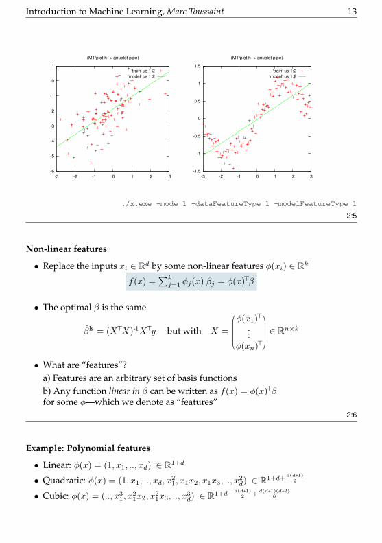
• Are these linear models? Linear in what?– Input: No.– Parameters, features: Yes!
2:1
Linear Modelling is more powerful than it might seem at first!
• Linear Regression on non-linear features → very powerful (polynomials, piece-wise,spline basis, kernels)
• Regularization (Ridge, Lasso) & cross-validation for proper generalization to test data• Gaussian Processes and SVMs are closely related (linear in kernel features, but with
different optimality criteria)• Liquid/Echo State Machines, Extreme Learning, are examples of linear modelling on
many (sort of random) non-linear features• Basic insights in model complexity (effective degrees of freedom)• Input relevance estimation (z-score) and feature selection (Lasso)• Linear regression→ linear classification (logistic regression: outputs are likelihood ra-
tios)
⇒ Linear modelling is a core of ML(We roughly follow Hastie, Tibshirani, Friedman: Elements of Statistical Learning)
2:2
Linear Regression
12 Introduction to Machine Learning, Marc Toussaint
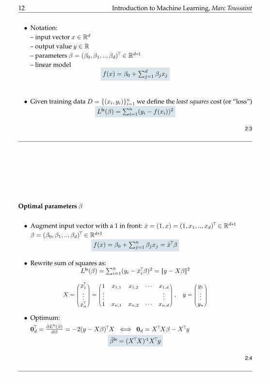
• Notation:– input vector x ∈ Rd
– output value y ∈ R– parameters β = (β0, β1, .., βd)
>∈ Rd+1
– linear modelf(x) = β0 +
∑dj=1 βjxj
• Given training data D = (xi, yi)ni=1 we define the least squares cost (or “loss”)
Lls(β) =∑ni=1(yi − f(xi))
2
2:3
Optimal parameters β
• Augment input vector with a 1 in front: x = (1, x) = (1, x1, .., xd)>∈ Rd+1
β = (β0, β1, .., βd)>∈ Rd+1
f(x) = β0 +∑nj=1 βjxj = x>β
• Rewrite sum of squares as:Lls(β) =
∑ni=1(yi − x>iβ)2 = ||y −Xβ||2
X =
x>1...x>n
=
1 x1,1 x1,2 · · · x1,d...
...1 xn,1 xn,2 · · · xn,d
, y =
y1...yn
• Optimum:
0>d = ∂Lls(β)∂β = −2(y −Xβ)>X ⇐⇒ 0d = X>Xβ −X>y
βls = (X>X)-1X>y
2:4
Introduction to Machine Learning, Marc Toussaint 13
-6
-5
-4
-3
-2
-1
0
1
-3 -2 -1 0 1 2 3
(MT/plot.h -> gnuplot pipe)
'train' us 1:2'model' us 1:2
-1.5
-1
-0.5
0
0.5
1
1.5
-3 -2 -1 0 1 2 3
(MT/plot.h -> gnuplot pipe)
'train' us 1:2'model' us 1:2
./x.exe -mode 1 -dataFeatureType 1 -modelFeatureType 1
2:5
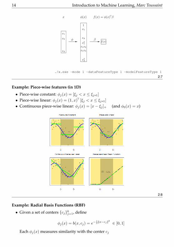
Non-linear features
• Replace the inputs xi ∈ Rd by some non-linear features φ(xi) ∈ Rk
f(x) =∑kj=1 φj(x) βj = φ(x)>β
• The optimal β is the same
βls = (X>X)-1X>y but with X =
φ(x1)>
...φ(xn)>
∈ Rn×k
• What are “features”?a) Features are an arbitrary set of basis functionsb) Any function linear in β can be written as f(x) = φ(x)>βfor some φ—which we denote as “features”
2:6
Example: Polynomial features
• Linear: φ(x) = (1, x1, .., xd) ∈ R1+d
• Quadratic: φ(x) = (1, x1, .., xd, x21, x1x2, x1x3, .., x
2d) ∈ R1+d+
d(d+1)2
• Cubic: φ(x) = (.., x31, x
21x2, x
21x3, .., x
3d) ∈ R1+d+
d(d+1)2 +
d(d+1)(d+2)6
14 Introduction to Machine Learning, Marc Toussaint
x1
x2
xd
φ β
1
x21
x1
xd
x1x2
x1x3
x2d
φ(x)x f(x) = φ(x)>β
f(x)
./x.exe -mode 1 -dataFeatureType 1 -modelFeatureType 1
2:7
Example: Piece-wise features (in 1D)
• Piece-wise constant: φj(x) = [ξj < x ≤ ξj+1]
• Piece-wise linear: φj(x) = (1, x)> [ξj < x ≤ ξj+1]
• Continuous piece-wise linear: φj(x) = [x− ξj ]+ (and φ0(x) = x)
2:8
Example: Radial Basis Functions (RBF)
• Given a set of centers cjkj=1, define
φj(x) = b(x, cj) = e−12 ||x−cj ||
2
∈ [0, 1]
Each φj(x) measures similarity with the center cj

Introduction to Machine Learning, Marc Toussaint 15
• Special case:use all training inputs xini=1 as centers
φ(x) =
1b(x, x1)
...b(x, xn)
(n+ 1 dim)
This is related to “kernel methods” and GPs, but not quite the same—we’ll discuss thislater.
2:9
Features
• Polynomial• Piece-wise• Radial basis functions (RBF)• Splines (see Hastie Ch. 5)
• Linear regression on top of rich features is extremely powerful!2:10
The need for regularization
Noisy sin data fitted with radial basis functions-1.5
-1
-0.5
0
0.5
1
1.5
2
-3 -2 -1 0 1 2 3
(MT/plot.h -> gnuplot pipe)
'z.train' us 1:2'z.model' us 1:2
./x.exe -mode 1 -n 40 -modelFeatureType 4 -dataType 2 -rbfWidth .1 -sigma
.5 -lambda 1e-10
• Overfitting & generalization:The model overfits to the data—and generalizes badly
• Estimator variance:When you repeat the experiment (keeping the underlying function fixed), theregression always returns a different model estimate
2:11
Estimator variance
• Assumptions:
– We computed parameters β = (X>X)-1X>y
– The data was noisy with variance Vary = σ2In
Then
16 Introduction to Machine Learning, Marc Toussaint
Varβ = (X>X)-1σ2
– high data noise σ→ high estimator variance
– more data→ less estimator variance: Varβ ∝ 1n
• In practise we don’t know σ, but we can estimate it based on the deviation fromthe learnt model: (with k = dim(β) = dim(φ))
σ2 =1
n− k
n∑i=1
(yi − f(xi))2
2:12
• If we could reduce the variance of the estimator, we could reduce overfitting—and increase generalization.• Hastie’s section on shrinkage methods is great! Describes several ideas on re-
ducing estimator variance by reducing model complexity. We focus on regu-larization.
2:13
Ridge regression: L2-regularization
• We add a regularization to the cost:
Lridge(β) =∑ni=1(yi − φ(xi)
>β)2 + λ∑kj=2 β
2j
NOTE: β1 is usually not regularized!
• Optimum:
βridge = (X>X + λI)-1X>y
(where I = Ik, or with I1,1 = 0 if β1 is not regularized)2:14
• The objective is now composed of two “potentials”: The loss, which dependson the data and jumps around (introduces variance), and the regularizationpenalty (sitting steadily at zero). Both are “pulling” at the optimal β → theregularization reduces variance.
• The estimator variance becomes less: Varβ = (X>X + λI)-1σ2
Introduction to Machine Learning, Marc Toussaint 17
• The ridge effectively reduces the complexity of the model:
df(λ) =∑dj=1
d2j
d2j+λ
where d2j is the eigenvalue of X>X = V D2V>
(details: Hastie 3.4.1)
2:15
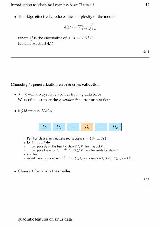
Choosing λ: generalization error & cross validation
• λ = 0 will always have a lower training data errorWe need to estimate the generalization error on test data
• k-fold cross-validation:
D1 D2 Di Dk· · · · · ·
1: Partition data D in k equal sized subsets D = D1, .., Dk2: for i = 1, .., k do3: compute βi on the training data D \Di leaving out Di4: compute the error `i = Lls(βi, Di)/|Di| on the validation data Di5: end for6: report mean squared error ˆ= 1/k
∑i `i and variance 1/(k-1)[(
∑i `
2i )− k ˆ2]
• Choose λ for which ˆ is smallest
2:16
quadratic features on sinus data:
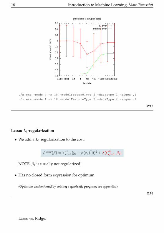
18 Introduction to Machine Learning, Marc Toussaint
0.4
0.5
0.6
0.7
0.8
0.9
1
1.1
1.2
1.3
0.001 0.01 0.1 1 10 100 1000 10000 100000
me
an
sq
ua
red
err
or
lambda
(MT/plot.h -> gnuplot pipe)
cv errortraining error
./x.exe -mode 4 -n 10 -modelFeatureType 2 -dataType 2 -sigma .1
./x.exe -mode 1 -n 10 -modelFeatureType 2 -dataType 2 -sigma .1
2:17
Lasso: L1-regularization
• We add a L1 regularization to the cost:
Llasso(β) =∑ni=1(yi − φ(xi)
>β)2 + λ∑kj=1 |βj |
NOTE: β1 is usually not regularized!
• Has no closed form expression for optimum
(Optimum can be found by solving a quadratic program; see appendix.)
2:18
Lasso vs. Ridge:
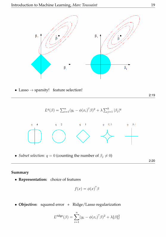
Introduction to Machine Learning, Marc Toussaint 19
• Lasso→ sparsity! feature selection!2:19
Lq(β) =∑ni=1(yi − φ(xi)
>β)2 + λ∑kj=1 |βj |q
• Subset selection: q = 0 (counting the number of βj 6= 0)2:20
Summary
• Representation: choice of features
f(x) = φ(x)>β
• Objective: squared error + Ridge/Lasso regularization
Lridge(β) =
n∑i=1
(yi − φ(xi)>β)2 + λ||β||2I

20 Introduction to Machine Learning, Marc Toussaint
• Solver: analytical (or quadratic program for Lasso)
βridge = (X>X + λI)-1X>y
2:21
Summary
• Linear models on non-linear features—extremely powerful
linearpolynomial
RBFkernel
RidgeLasso
regressionclassification*
*logistic regression
• Generalization ↔ Regularization ↔ complexity/DoF penalty
• Cross validation to estimate generalization empirically→ use to choose regu-larization parameters
2:22
Appendix: Dual formulation of Ridge
• The standard way to write the Ridge regularization:Lridge(β) =
∑ni=1(yi − φ(xi)
>β)2 + λ∑kj=1 β
2j
• Finding βridge = argminβ Lridge(β) is equivalent to solving
βridge = argminβ
n∑i=1
(yi − φ(xi)>β)2
subject tok∑j=1
β2j ≤ t
λ is the Lagrange multiplier for the inequality constraint2:23
Appendix: Dual formulation of Lasso
• The standard way to write the Lasso regularization:Llasso(β) =
∑ni=1(yi − φ(xi)
>β)2 + λ∑kj=1 |βj |
Introduction to Machine Learning, Marc Toussaint 21
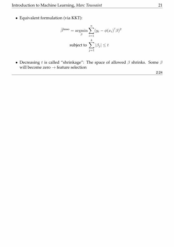
• Equivalent formulation (via KKT):
βlasso = argminβ
n∑i=1
(yi − φ(xi)>β)2
subject tok∑j=1
|βj | ≤ t
• Decreasing t is called “shrinkage”: The space of allowed β shrinks. Some βwill become zero→ feature selection
2:24

22 Introduction to Machine Learning, Marc Toussaint
3 Classification - Part 1
Discriminative Function
• Represent a discrete-valued function F : Rn → Y via a discriminative func-tion
f : Rn × Y → R
such thatF : x 7→ argmaxy f(x, y)
That is, a discriminative function f(x, y) maps an input x to an output
y(x) = argmaxy
f(x, y)
• A discriminative function f(x, y) has high value if y is a correct answer to x;and low value if y is a false answer• In that way a discriminative function e.g. discriminates correct sequence/image/graph-
labelling from wrong ones3:1
Example Discriminative Function
• Input: x ∈ R2; output y ∈ 1, 2, 3displayed are p(y=1|x), p(y=2|x), p(y=3|x)
0.9 0.5 0.1 0.9 0.5 0.1 0.9 0.5 0.1
-2-1
0 1
2 3 -2
-1 0
1 2
3
0
0.2
0.4
0.6
0.8
1
3:2
How could we parameterize a discriminative function?

Introduction to Machine Learning, Marc Toussaint 23
• Well, linear in features!
f(x, y) =∑kj=1 φj(x, y)βj = φ(x, y)>β
• Example: Let x ∈ R and y ∈ 1, 2, 3. Typical features might be
φ(x, y) =
1 [y = 1]x [y = 1]x2 [y = 1]1 [y = 2]x [y = 2]x2 [y = 2]1 [y = 3]x [y = 3]x2 [y = 3]
• Example: Let x, y ∈ 0, 1 be both discrete. Features might be
φ(x, y) =
1[x = 0][y = 0][x = 0][y = 1][x = 1][y = 0][x = 1][y = 1]
3:3
more intuition...
• Features “connect” input and output. Each φj(x, y) allows f to capture a cer-tain dependence between x and y• If both x and y are discrete, a feature φj(x, y) is typically a joint indicator func-
tion (logical function), indicating a certain “event”• Each weight βj mirrors how important/frequent/infrequent a certain depen-
dence described by φj(x, y) is• −f(x, y) is also called energy, and the following methods are also called energy-
based modelling, esp. in neural modelling
3:4
Logistic Regression

24 Introduction to Machine Learning, Marc Toussaint
-2
-1
0
1
2
3
-2 -1 0 1 2 3
(MT/plot.h -> gnuplot pipe)
train
decision boundary
• Input x ∈ R2
Output y ∈ 0, 1Example shows RBF Ridge Logistic Regression
3:5
A Loss Function for Classification
• Data D = (xi, yi)ni=1 with xi ∈ Rd and yi ∈ 0, 1
• Maximum likelihood:We interpret the discriminative function f(x, y) as defining class probabilities
p(y |x) = ef(x,y)∑y′ e
f(x,y′)
→ p(y |x) should be high for the correct class, and low otherwise
For each (xi, yi) we want to maximize the likelihood p(yi |xi):
Lneg-log-likelihood(β) = −∑ni=1 log p(yi |xi)
3:6
Logistic Regression: Binary Case
• In the binary case, we have “two functions” f(x, 0) and f(x, 1). W.l.o.g. we may fixf(x, 0) = 0 to zero. Therefore we choose features
φ(x, y) = φ(x) [y = 1]
with arbitrary input features φ(x) ∈ Rk
• We have
f(x, 1) = φ(x)>β , y = argmaxy
f(x, y) =
0 else1 if φ(x)>β > 0
Introduction to Machine Learning, Marc Toussaint 25
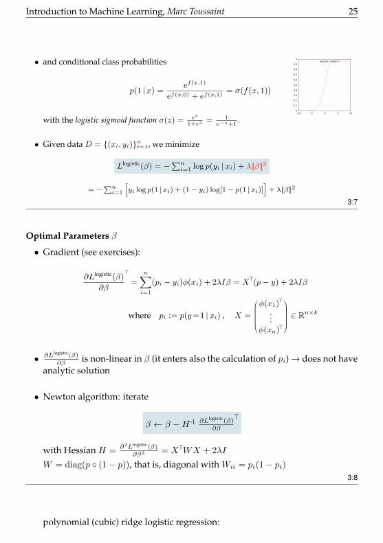
• and conditional class probabilities
p(1 |x) =ef(x,1)
ef(x,0) + ef(x,1)= σ(f(x, 1))
0
0.1
0.2
0.3
0.4
0.5
0.6
0.7
0.8
0.9
1
-10 -5 0 5 10
exp(x)/(1+exp(x))
with the logistic sigmoid function σ(z) = ez
1+ez= 1
e−z+1.
• Given data D = (xi, yi)ni=1, we minimize
Llogistic(β) = −∑ni=1 log p(yi |xi) + λ||β||2
= −∑ni=1
[yi log p(1 |xi) + (1− yi) log[1− p(1 |xi)]
]+ λ||β||2
3:7
Optimal Parameters β
• Gradient (see exercises):
∂Llogistic(β)
∂β
>
=
n∑i=1
(pi − yi)φ(xi) + 2λIβ = X>(p− y) + 2λIβ
where pi := p(y=1 |xi) , X =
φ(x1)>
...φ(xn)>
∈ Rn×k
• ∂Llogistic(β)∂β is non-linear in β (it enters also the calculation of pi)→ does not have
analytic solution
• Newton algorithm: iterate
β ← β −H -1 ∂Llogistic(β)∂β
>
with Hessian H = ∂2Llogistic(β)∂β2 = X>WX + 2λI
W = diag(p (1− p)), that is, diagonal with Wii = pi(1− pi)3:8
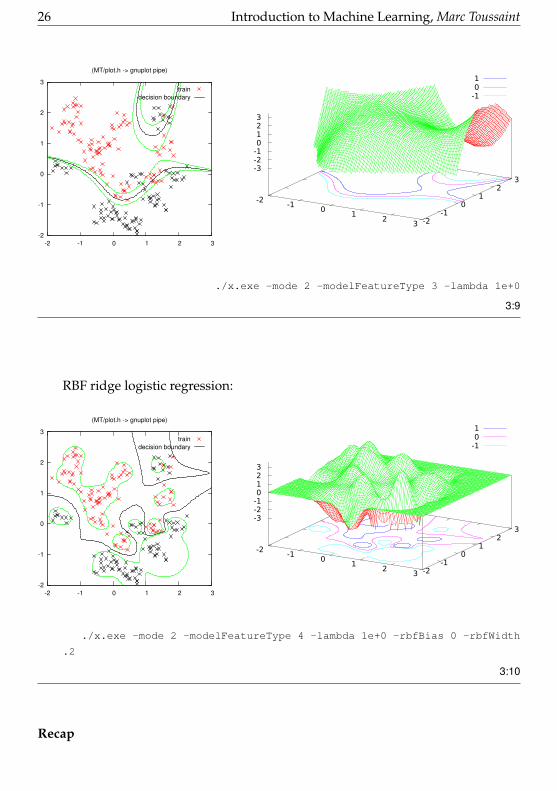
polynomial (cubic) ridge logistic regression:
26 Introduction to Machine Learning, Marc Toussaint
-2
-1
0
1
2
3
-2 -1 0 1 2 3
(MT/plot.h -> gnuplot pipe)
traindecision boundary
1 0 -1
-2-1
0 1
2 3 -2
-1 0
1 2
3
-3-2-1 0 1 2 3
./x.exe -mode 2 -modelFeatureType 3 -lambda 1e+0
3:9
RBF ridge logistic regression:
-2
-1
0
1
2
3
-2 -1 0 1 2 3
(MT/plot.h -> gnuplot pipe)
traindecision boundary
1 0 -1
-2-1
0 1
2 3 -2
-1 0
1 2
3
-3-2-1 0 1 2 3
./x.exe -mode 2 -modelFeatureType 4 -lambda 1e+0 -rbfBias 0 -rbfWidth
.2
3:10
Recap
Introduction to Machine Learning, Marc Toussaint 27
ridge regression logistic regressionREPRESENTATION f(x) = φ(x)>β f(x, y) = φ(x, y)>β
OBJECTIVE Lls(β) =∑ni=1(yi − f(xi))
2 + λ||β||2ILnll(β) =−∑ni=1 log p(yi |xi) + λ||β||2I
p(y |x) ∝ ef(x,y)
SOLVER βridge = (X>X + λI)-1X>y binary case:β ← β − (X>WX + 2λI)-1
(X>(p− y) + 2λIβ)
3:11
Logistic Regression: Multi-Class Case
• Data D = (xi, yi)ni=1 with xi ∈ Rd and yi ∈ 1, ..,M• We choose f(x, y) = φ(x, y)>β with
φ(x, y) =
φ(x) [y = 1]φ(x) [y = 2]
...φ(x) [y = M ]
where φ(x) are arbitrary features. We have M -1 parameters β• Conditional class probabilties
p(y |x) =ef(x,y)∑y′ e
f(x,y′)
• Given data D = (xi, yi)ni=1, we minimize
Llogistic(β) = −∑ni=1 log p(y=yi |xi) + λ||β||2
3:12
Optimal Parameters β
• Gradient:∂Llogistic(β)
∂βc
>=∑ni=1(pic−yic)φ(xi)+2λIβc = X>(pc−yc)+2λIβc , pic = p(y=
c |xi)
• Hessian: H = ∂2Llogistic(β)∂βc∂βd
= X>WcdX + 2[c = d] λI
Wcd diagonal with Wcd,ii = pic([c = d]− pid)3:13
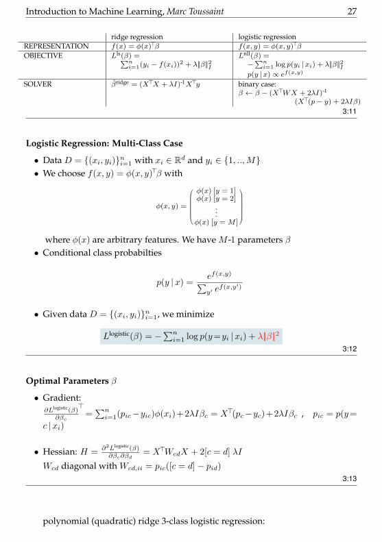
polynomial (quadratic) ridge 3-class logistic regression:
28 Introduction to Machine Learning, Marc Toussaint
-2
-1
0
1
2
3
-2 -1 0 1 2 3
(MT/plot.h -> gnuplot pipe)
trainp=0.5
0.9 0.5 0.1 0.9 0.5 0.1 0.9 0.5 0.1
-2-1
0 1
2 3 -2
-1 0
1 2
3
0
0.2
0.4
0.6
0.8
1
./x.exe -mode 3 -modelFeatureType 3 -lambda 1e+1
3:14
Summary
• Logistic regression belongs to the class of probabilistic classification approaches.The basic idea is estimating the class probabilities using a logistic function.• There are many other non-probabilistic approaches. One of the most important
classifier there is the support vector machines.3:15
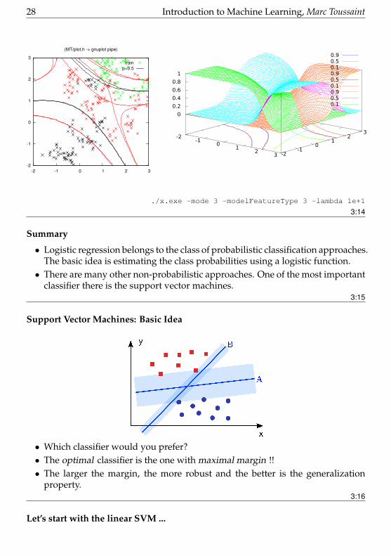
Support Vector Machines: Basic Idea
• Which classifier would you prefer?• The optimal classifier is the one with maximal margin !!• The larger the margin, the more robust and the better is the generalization
property.3:16
Let’s start with the linear SVM ...

Introduction to Machine Learning, Marc Toussaint 29
• Find a linear surface which maximizes the margin
Thus,minβ
12 ‖ β ‖
2, s.t. yi(xTi β + β0) ≥ 1
yi ∈ −1, 1 ... outputs, i = 1...N
Decision functiony(x)=sign
(xTβ∗+β∗0
)3:17
Dual Representation of the linear SVM
Lagrangian function
J(β, β0, α) =1
2‖ β ‖2 −
N∑i=1
αi[yi(x
Ti β + β0)− 1
]Dual representation
maxαQ(α) =∑Ni=1 αi −
12
∑Ni=1
∑Nj=1 αiαjyiyjx
Ti xj
s.t.∑Ni=1 αiyi = 0; αi ≥ 0 for i = 1, 2, · · · , N
• The optimization of the dual form is convex• The input patterns appear as dot products
3:18
30 Introduction to Machine Learning, Marc Toussaint
4 Classification - Part 2
Recap: Linear SVM
• Find a linear surface which maximizes the margin
Thus,minβ
12 ‖ β ‖
2, s.t. yi(xTi β + β0) ≥ 1
yi ∈ −1, 1 ... outputs, i = 1...N
• All training examples need to be correctly classified !!• What happens when training examples are not linearly separable?
4:1
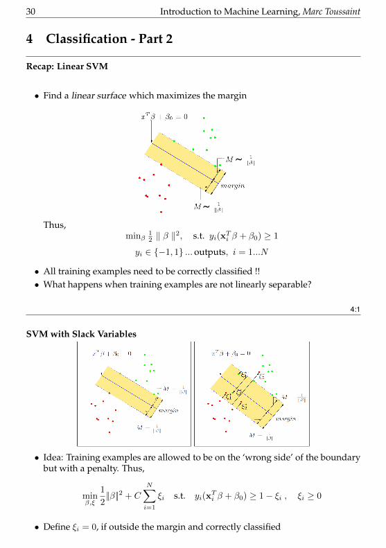
SVM with Slack Variables
• Idea: Training examples are allowed to be on the ‘wrong side’ of the boundarybut with a penalty. Thus,
minβ,ξ
1
2||β||2 + C
N∑i=1
ξi s.t. yi(xTi β + β0) ≥ 1− ξi , ξi ≥ 0
• Define ξi = 0, if outside the margin and correctly classified
Introduction to Machine Learning, Marc Toussaint 31
• Define ξi = |yi − (xTi β + β0)| for other points→ 0 < ξi ≤ 1, if inside the margin but on the correct side of boundary→ ξi > 1,if wrong side of boundary
4:2
Dual Representation
Lagrangian function
J(β, β0, α, µ) =1
2‖ β ‖2 +C
N∑i=1
ξi −N∑i=1
αi[yi(x
Ti β + β0)− 1 + ξi
]−
N∑i=1
µiξi
Dual representation
maxαQ(α) =∑Ni=1 αi −
12
∑Ni=1
∑Nj=1 αiαjyiyjx
Ti xj
s.t.∑Ni=1 αiyi = 0; C ≥ αi ≥ 0 for i = 1, 2, · · · , N
• This is identical to the linearly separable case, except that we now have boxconstraints on αi.
4:3
Summary Linear SVM
• The dual parameters αi indicate whether the constraint yi(xTi β + β0) is active.The dual problem is convex• For all inactive constraints, i.e. ξi = 0, the data point (xi, yi) does not directly
influence the solution• Inactive points/constraints have αi = 0, active points/constraints have αi 6= 0.
Active points are support vectors, resulting in a sparse solution for the decisionboundary
• With β =∑Ni=1 αiyixi, we have the prediction
y(x)=sign
(M∑i=1
αiyixTi x+β∗0
)where M ≤ N is number of support vectors
4:4
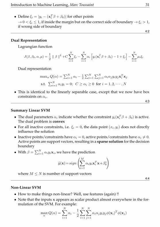
Non-Linear SVM
• How to make things non-linear? Well, use features (again) !!• Note that the inputs x appears as scalar product almost everywhere in the for-
mulation of the SVM. For example:
maxα
Q(α) =
N∑i=1
αi −1
2
N∑i=1
N∑j=1
αiαjyiyjφ(xi)Tφ(xj)
32 Introduction to Machine Learning, Marc Toussaint
• We have the prediction
y(x)=sign
(N∑i=1
αiyiφ(xi)Tφ(x)+β∗0
)
• Now, define a kernel function
k(xi,xj) = φ(xi)Tφ(xj)
• This is a very powerful way to make things non-linear. This is the so-calledkernel trick.
4:5
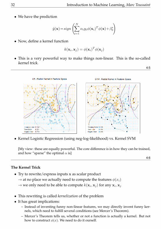
• Kernel Logistic Regression (using neg-log-likelihood) vs. Kernel SVM
[My view: these are equally powerful. The core difference is in how they can be trained,and how “sparse” the optimal α is]
4:6
The Kernel Trick
• Try to rewrite/express inputs x as scalar product→ at no place we actually need to compute the features φ(xi)
→we only need to be able to compute k(xi,xj) for any xi,xj
• This rewriting is called kernelization of the problem• It has great implications:
– Instead of inventing funny non-linear features, we may directly invent funny ker-nels, which need to fulfill several conditions (see Mercer’s Theorem).
– Mercer’s Theorem tells us, whether or not a function is actually a kernel. But nothow to construct φ(x). We need to do it ourself.
Introduction to Machine Learning, Marc Toussaint 33
– Inventing a kernel is intuitive: k(xi,xj) expresses how correlated yi and yj shouldbe. This is a meassure of similarity, it compares xi and xj . Specifying how ’com-parable’ xi and xj are is often more intuitive than defining “features that mightwork”
4:7
An Example for Kernelization:Kernel Ridge Regression
• Reconsider solution of Ridge regression (using the Woodbury identity):βridge = (X>X + λIk)-1X>y = X>(XX>+ λIn)-1y
• Recall X>= (φ(x1), .., φ(xn)) ∈ Rk×n, then:
f ridge(x) = φ(x)>βridge = φ(x)>X>︸ ︷︷ ︸κ(x)>
(XX>︸ ︷︷ ︸K
+λI)-1y
K is called kernel matrix and has elements
Kij = k(xi, xj) := φ(xi)>φ(xj)
κ is the vector: κ(x)>= φ(x)>X>= k(x, x1:n)
The kernel function k(x, x′) calculates the scalar product in feature space.4:8
• Every choice of features implies a kernel.
• Every choice of kernel corresponds to a specific choice of features.4:9
Example Kernels
• Kernel functions need to be positive definite: ∀z:|z|>0 : k(z, z′) > 0
• Examples:– Polynomial: k(x, x′) = (x>x′ + c)d
Let’s verify for d = 2, φ(x) =(1,√
2x1,√
2x2, x21,√
2x1x2, x22
)>.
– Squared exponential (radial basis function): k(x, x′) = exp(−γ |x− x′ | 2). Find thecorresponding feature function.
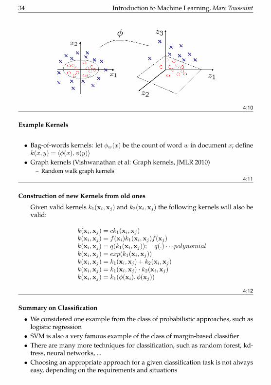
34 Introduction to Machine Learning, Marc Toussaint
4:10
Example Kernels
• Bag-of-words kernels: let φw(x) be the count of word w in document x; definek(x, y) = 〈φ(x), φ(y)〉• Graph kernels (Vishwanathan et al: Graph kernels, JMLR 2010)
– Random walk graph kernels4:11
Construction of new Kernels from old ones
Given valid kernels k1(xi,xj) and k2(xi,xj) the following kernels will also bevalid:
k(xi,xj) = ck1(xi,xj)k(xi,xj) = f(xi)k1(xi,xj)f(xj)k(xi,xj) = q(k1(xi,xj)); q(.) · · · polynomialk(xi,xj) = exp(k1(xi,xj))k(xi,xj) = k1(xi,xj) + k2(xi,xj)k(xi,xj) = k1(xi,xj) · k2(xi,xj)k(xi,xj) = k1(φ(xi), φ(xj))
4:12
Summary on Classification
• We considered one example from the class of probabilistic approaches, such aslogistic regression• SVM is also a very famous example of the class of margin-based classifier• There are many more techniques for classification, such as random forest, kd-
tress, neural networks, ...• Choosing an appropriate approach for a given classification task is not always
easy, depending on the requirements and situations
Introduction to Machine Learning, Marc Toussaint 35
• Making things non-linear can be done by introducing features. The most ele-gant way to do this is the formulation of kernels.
4:13
36 Introduction to Machine Learning, Marc Toussaint
5 Unsupervised Learning - Part 1
Unsupervised Learning
• What does that mean? Generally: modelling P (x)
• Examples:– Finding lower-dimensional spaces
– Clustering
– Density estimation
– Fitting a graphical model
• “Supervised Learning as special case”...5:1
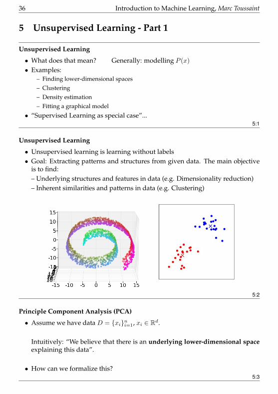
Unsupervised Learning
• Unsupervised learning is learning without labels• Goal: Extracting patterns and structures from given data. The main objective
is to find:– Underlying structures and features in data (e.g. Dimensionality reduction)– Inherent similarities and patterns in data (e.g. Clustering)
5:2
Principle Component Analysis (PCA)
• Assume we have data D = xini=1, xi ∈ Rd.
Intuitively: “We believe that there is an underlying lower-dimensional spaceexplaining this data”.
• How can we formalize this?5:3
Introduction to Machine Learning, Marc Toussaint 37
PCA: Minimizing Projection Error
• For each xi ∈ Rd we postulate a lower-dimensional latent variable zi ∈ Rp,where p ≤ d
xi ≈ Vpzi + µ
• Optimality: Find Vp, µ and values zi that minimize the projection error
n∑i=1
||xi − (Vpzi + µ)||2
5:4
Find Optimal Vp
µ, z1:n = argminµ,z1:n
n∑i=1
||xi − Vpzi − µ||2
⇒ µ = 〈xi〉 = 1n
∑ni=1 xi , zi = V>p (xi − µ)
• Center the data xi = xi − µ. Then
Vp = argminVp
n∑i=1
||xi − VpV>p xi||2
• Solution via Singular Value Decomposition:– Compute the covariance matrix Sx = XTX , where X ∈ Rn×d be the centereddata matrix containing all xi– Do a eigenvalue decomposition Sx = V DV T , D = diag(σ1, σ2, ..., σd)
– Select the p largest σi and corresponding ViVp := V1:d,1:p = (v1 v2 · · · vp)
5:5
38 Introduction to Machine Learning, Marc Toussaint
Some Remarks for PCA
• V>p is the matrix that projects to the largest variance directions of X>X• Equivalent PCA formulation: Maximum variance formulation
v1 = argmaxv1
1
n
n∑i=1
(v>1xi − v>1µ)2
• Generally: Apply ML method on top of Z instead of X by doing the transfor-mation first
Z = XVp
5:6
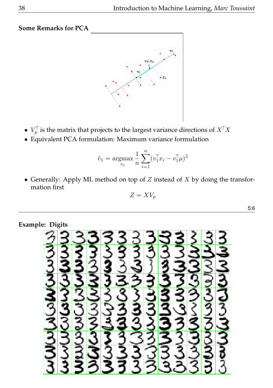
Example: Digits
Introduction to Machine Learning, Marc Toussaint 39
5:7
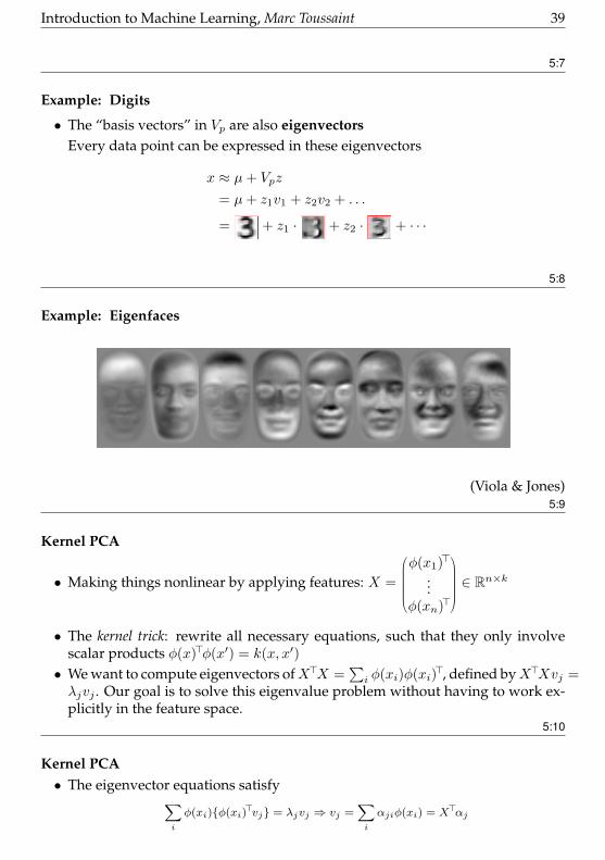
Example: Digits
• The “basis vectors” in Vp are also eigenvectorsEvery data point can be expressed in these eigenvectors
x ≈ µ+ Vpz
= µ+ z1v1 + z2v2 + . . .
= + z1 · + z2 · + · · ·
5:8
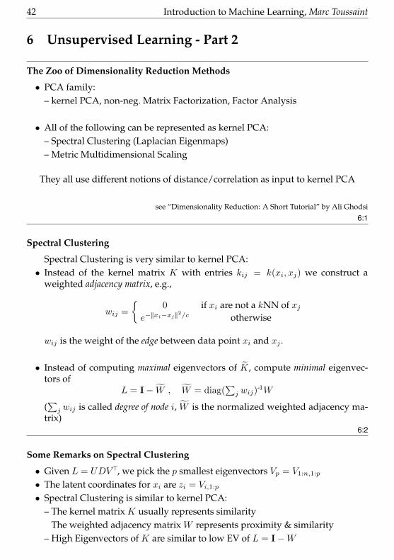
Example: Eigenfaces
(Viola & Jones)5:9
Kernel PCA
• Making things nonlinear by applying features: X =
φ(x1)>
...φ(xn)>
∈ Rn×k
• The kernel trick: rewrite all necessary equations, such that they only involvescalar products φ(x)>φ(x′) = k(x, x′)
• We want to compute eigenvectors ofX>X =∑i φ(xi)φ(xi)
>, defined byX>Xvj =λjvj . Our goal is to solve this eigenvalue problem without having to work ex-plicitly in the feature space.
5:10
Kernel PCA• The eigenvector equations satisfy∑
i
φ(xi)φ(xi)>vj = λjvj ⇒ vj =
∑i
αjiφ(xi) = X>αj

40 Introduction to Machine Learning, Marc Toussaint
• Substituting this into the eigenvector equation
X>Xvj = λvj
XX>︸ ︷︷ ︸K
Xvj︸︷︷︸Kαj
= λXvj︸︷︷︸Kαj
Kαj = λαj
Now we have eigenvector problems depending only on kernel matrices, whereK = XX>with entries Kij = k(xi, xj)
→We compute SVD of the kernel matrix K→ gives eigenvectors αj ∈ Rn.
• We can also “center” the feature space by K = (I− 1n11
>)K(I− 1n11
>)
• Projection:x 7→ z = V>p φ(x) =
∑i
α1:p,iφ(xi)>φ(x) = Aκ(x)
with matrix A ∈ Rp×n, Aji = αji and vector κ(x) ∈ Rn, κi(x) = k(xi, x)
5:11
Kernel PCA
• Kernel PCA uncovers quite surprising structure:
While PCA “merely” picks high-variance dimensionsKernel PCA picks high variance features—where features correspond to basisfunctions over x
• Kernel PCA may map data xi to latent coordinates zi where clustering is mucheasier
• All of the following can be represented as kernel PCA:– Local Linear Embedding– Metric Multidimensional Scaling– Laplacian Eigenmaps (Spectral Clustering)
see “Dimensionality Reduction: A Short Tutorial” by Ali Ghodsi
5:12
Kernel PCA
red points: datagreen shading: eigenvector αj represented as functions
∑i αjik(xj , x)

Introduction to Machine Learning, Marc Toussaint 41
Kernel PCA “coordinates” allow us to discriminate clusters!5:13
Kernel PCA clustering
• Using a kernel function k(x, x′) = e−||x−x′||2/c:
• Gaussian mixtures or k-means will easily cluster this5:14
42 Introduction to Machine Learning, Marc Toussaint
6 Unsupervised Learning - Part 2
The Zoo of Dimensionality Reduction Methods
• PCA family:– kernel PCA, non-neg. Matrix Factorization, Factor Analysis
• All of the following can be represented as kernel PCA:– Spectral Clustering (Laplacian Eigenmaps)– Metric Multidimensional Scaling
They all use different notions of distance/correlation as input to kernel PCA
see “Dimensionality Reduction: A Short Tutorial” by Ali Ghodsi6:1
Spectral Clustering
Spectral Clustering is very similar to kernel PCA:• Instead of the kernel matrix K with entries kij = k(xi, xj) we construct a
weighted adjacency matrix, e.g.,
wij =
0 if xi are not a kNN of xj
e−||xi−xj ||2/c otherwise
wij is the weight of the edge between data point xi and xj .
• Instead of computing maximal eigenvectors of K, compute minimal eigenvec-tors of
L = I− W , W = diag(∑j wij)
-1W
(∑j wij is called degree of node i, W is the normalized weighted adjacency ma-
trix)6:2
Some Remarks on Spectral Clustering
• Given L = UDV>, we pick the p smallest eigenvectors Vp = V1:n,1:p
• The latent coordinates for xi are zi = Vi,1:p
• Spectral Clustering is similar to kernel PCA:– The kernel matrix K usually represents similarity
The weighted adjacency matrix W represents proximity & similarity– High Eigenvectors of K are similar to low EV of L = I−W

Introduction to Machine Learning, Marc Toussaint 43
• Original interpretation of Spectral Clustering:– L = I−W (weighted graph Laplacian) describes a diffusion process:
The diffusion rate Wij is high if i and j are close and similar– Eigenvectors of L correspond to stationary solutions
6:3
Metric Multidimensional Scaling
• Assume we have data D = xini=1, xi ∈ Rd.As before we want to indentify latent lower-dimensional representations zi ∈Rp for this data.
• A simple idea: Minimize the stress
SC(z1:n) =∑i 6=j(d
2ij − ||zi − zj ||2)2
where d2ij = ||xi − xj ||2
⇒ We want distances in high-dimensional space to be equal to distances inlow-dimensional space.
6:4
Metric Multidimensional Scaling = (kernel) PCA
• Note the relation:
d2ij = ||xi − xj ||2 = ||xi − x||2 + ||xj − x||2 − 2(xi − x)>(xj − x)
This translates a distance into a (centered) scalar product
• If may we defineK = (I− 1
n11>)D(I− 1
n11>) , Dij = −d2
ij/2
then Kij = (xi− x)>(xj− x) is the normal covariance matrix and MDS is equiv-alent to kernel PCA• The solution is Z = XVp, where Vp is the matrix of p eigenvectors with highest
eigenvalues6:5
Clustering
• Divide a set of objects / data points into clusters. Objects in the same clustersare similar to each other.• Clustering often involves two steps: (i) Map the data to some embedding that
emphasizes clusters, (ii) Explicitly analyze clusters.• Applications:
44 Introduction to Machine Learning, Marc Toussaint
– Data reduction⇒ “Compression” through data representation
– Find informative patterns⇒ Extract useful data classes
– Outlier detection⇒ Identify unusual data objects
• Many clustering methods available, e.g.:– k-means clustering
– Gaussian Mixture Model
– Agglomerative Clustering6:6
k-means Clustering
• Idea: Assign N data points xn to K clusters, while minimizing the objectivefunction J
minrnk,µk
J =
N∑n=1
K∑k=1
rnk ‖ xn − µk ‖2
where rnk ∈ 0, 1 ... indicator variable, µk ... center of the cluster• Solving this problem results in a two-stage optimization:
– Initialization of K cluster centers µk (e.g. random)
– Fixing µk and minimizing J w.r.t. rnk
rnk =
1 if k = argmin
k‖ xn − µk ‖2
0 otherwise
⇒ Assign the nth data point to the closest cluster center
– Fixing rnk and minimizing J w.r.t. µk
µk =
∑n rnkxn∑n rnk
⇒ Compute new cluster centers as the mean of cluster’s members
– Iterating the steps until convergence6:7
k-means Clustering6:8
Remarks on k-means Clustering
• Converges to local minimum→many restarts• Choosing K?
– Plot L(K) = minrnk,µk J for different K
– Choose a tradeoff between model complexity (large K) and data fit (small lossL(K))
• Very efficient algorithm, k-means work well for large data6:9
Introduction to Machine Learning, Marc Toussaint 45
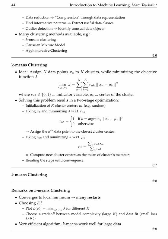
Gaussian Mixture Model for Clustering
• Idea: Approximate the “true” distribution, from which the data xiNi=1 is gen-erated, using a mixture of multivariate Gaussians, i.e.
p(x) =
K∑k=1
πk N(x|µk,Σk)
where πk is the mixing value, with 0 ≤ πk ≤ 1 and∑Kk=1 πk = 1
• Maximize the resulting log-likelihood
maxπ,µ,Σ
ln p(X|π, µ,Σ) =
N∑i=1
ln
[K∑k=1
πk N(xi|µk,Σk)
]
6:10
Gaussian Mixture Model: Algorithm
• Initialize the centers µ1:K randomly from the data; all covariances Σ1:K to unitand all πk uniformly.• Evaluate the posterior probability γik that point xi belongs to cluster k:
γik =πkN(xi|µk,Σk)∑Kj=1 πjN(xi|µj ,Σj)
• Update the estimates:
πk =NkN
46 Introduction to Machine Learning, Marc Toussaint
µk =1
Nk
∑Ni γik xi
Σk =1
Nk
∑Ni γik (xi − µk)(xi − µk)>
where Nk =∑i γik
6:11
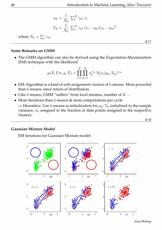
Some Remarks on GMM
• The GMM algorithm can also be derived using the Expectation-Maximization(EM) technique with the likelihood
p(X,Γ|π, µ,Σ) =
N∏i=1
K∏k=1
πγikk N(xi|µk,Σk)γik
• EM-Algorithm is a kind of soft-assignment version of k-means. More powerfulthan k-means, since return of distribution.• Like k-means, GMM “suffers” from local minima, number of K ...• More iterations than k-means & more computations per cycle⇒ Heuristics: Use k-means as initialization for µk; Σk initialized to the samplevariance; πk assigned to the fraction of data points assigned to the respectiveclusters.
6:12
Gaussian Mixture Model
EM iterations for Gaussian Mixture model:
from Bishop

Introduction to Machine Learning, Marc Toussaint 47
6:13
Agglomerative Hierarchical Clustering
• agglomerative = bottom-up, divisive = top-down• Merge the two groups with the smallest intergroup dissimilarity• Dissimilarity of two groups G, H can be measures as
– Nearest Neighbor (or “single linkage”): d(G,H) = mini∈G,j∈H d(xi, xj)
– Furthest Neighbor (or “complete linkage”): d(G,H) = maxi∈G,j∈H d(xi, xj)
– Group Average: d(G,H) = 1|G||H|
∑i∈G
∑j∈H d(xi, xj)
6:14
Agglomerative Hierarchical Clustering
6:15
48 Introduction to Machine Learning, Marc Toussaint
7 The Breadth of MLNeural Networks & Deep Learning
Neural Networks
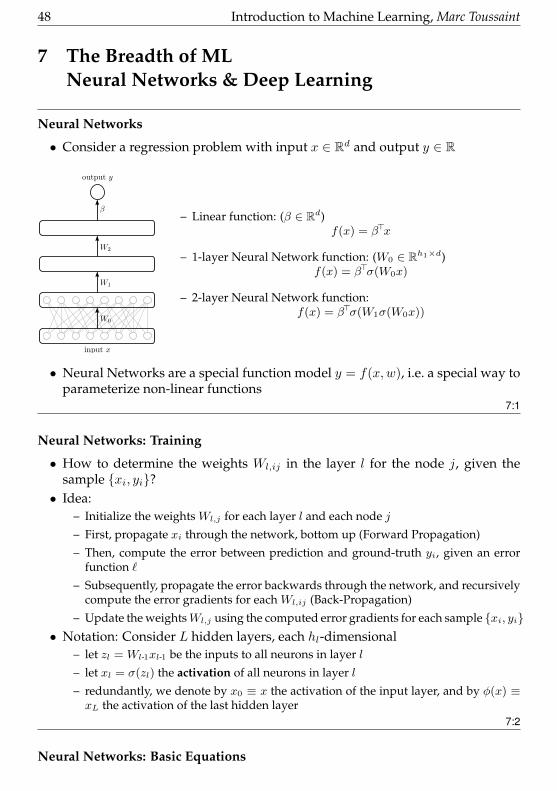
• Consider a regression problem with input x ∈ Rd and output y ∈ R
– Linear function: (β ∈ Rd)f(x) = β>x
– 1-layer Neural Network function: (W0 ∈ Rh1×d)f(x) = β>σ(W0x)
– 2-layer Neural Network function:f(x) = β>σ(W1σ(W0x))
• Neural Networks are a special function model y = f(x,w), i.e. a special way toparameterize non-linear functions
7:1
Neural Networks: Training
• How to determine the weights Wl,ij in the layer l for the node j, given thesample xi, yi?• Idea:
– Initialize the weights Wl,j for each layer l and each node j
– First, propagate xi through the network, bottom up (Forward Propagation)
– Then, compute the error between prediction and ground-truth yi, given an errorfunction `
– Subsequently, propagate the error backwards through the network, and recursivelycompute the error gradients for each Wl,ij (Back-Propagation)
– Update the weightsWl,j using the computed error gradients for each sample xi, yi• Notation: Consider L hidden layers, each hl-dimensional
– let zl = Wl-1xl-1 be the inputs to all neurons in layer l
– let xl = σ(zl) the activation of all neurons in layer l
– redundantly, we denote by x0 ≡ x the activation of the input layer, and by φ(x) ≡xL the activation of the last hidden layer
7:2
Neural Networks: Basic Equations
Introduction to Machine Learning, Marc Toussaint 49
• Forward propagation: An L-layer NN recursively computes, for l = 1, .., L,
∀l=1,..,L : zl = Wl-1xl-1 , xl = σ(zl)
and then computes the output f ≡ zL+1 = WLxL
• Backpropagation: Given some loss `(f), let δL+1∆= ∂`
∂f. We can recursivly compute the
loss-gradient w.r.t. the inputs of layer l:
∀l=L,..,1 : δl∆=d`
dzl=
d`
dzl+1
∂zl+1∂xl
∂xl∂zl
= [δl+1 Wl] [xl (1− xl)]>
where is an element-wise product. The gradient w.r.t. weights is:
d`
dWl,ij=
d`
dzl+1,i
∂zl+1,i∂Wl,ij
= δl+1,i xl,j ord`
dWl= δ>l+1x
>l
• Weight-update:– many ways of different weight-updates possible, given gradients d`
dWl
– for example, the delta rule: Wnewl = W old
l + ∆Wl = W oldl − η d`
dWl
7:3
Neural Networks: Regression
• In the standard regression case, y ∈ R, we typically assume a squared errorloss `(f) =
∑i(f(xi, w)− yi)2. We have
δL+1 =∑i
2(f(xi, w)− yi)>
• Regularization: Add a L2 or L1 regularization. First compute all gradients asbefore, then add λWl,ij (for L2), or λ signWl,ij (for L1) to the gradient. His-torically, this is called weight decay, as the additional gradient leads to a stepdecaying the weighs.• The optimal output weights are as for standard regression
W ∗L = (X>X + λI)-1X>y
where X is the data matrix of activations xL ≡ φ(x)7:4
Neural Networks: Classification
• Consider the multi-class case y ∈ 1, ..,M. Then we have M output neuronsto represent the discriminative function
f(x, y, w) = (W>LzL)y , W ∈ RM×hL
• Choosing neg-log-likelihood objective↔ logistic regression• Choosing hinge loss objective↔ “NN + SVM”
50 Introduction to Machine Learning, Marc Toussaint
– For given x, let y∗ be the correct class. The one-vs-all hinge loss is:∑y 6=y∗ max0, 1− (fy∗ − fy)
– For output neuron y 6= y∗ this implies a gradient δy = [fy∗ < fy + 1]
– For output neuron y∗ this implies a gradient δy∗ = −∑y 6=y∗ [fy∗ < fy + 1]
Only data points inside the margin induce an error (and gradient).
– This is also called Perceptron Algorithm7:5
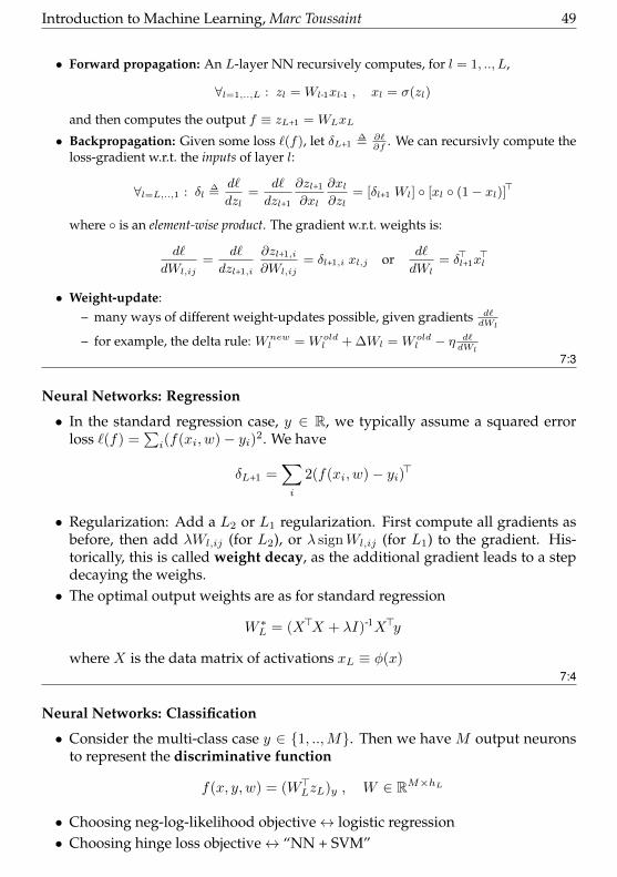
Neural Networks: Dimensionality Reduction
• Dimensionality reduction can be performed with autoencoders• An autoencoder typically is a NN of the type
which is trained to reproduce the input: mini ||y(xi)− xi||2
The hidden layer (“bottleneck”) needs to find a good representation/compression.
• Similar to the PCA objective, but nonlinear
• Stacking autoencoders (Deep Autoencoders):
7:6
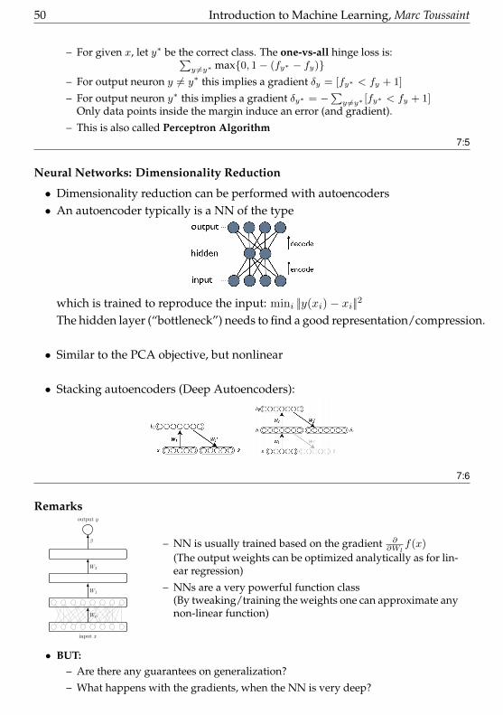
Remarks
– NN is usually trained based on the gradient ∂∂Wl
f(x)
(The output weights can be optimized analytically as for lin-ear regression)
– NNs are a very powerful function class(By tweaking/training the weights one can approximate anynon-linear function)
• BUT:– Are there any guarantees on generalization?
– What happens with the gradients, when the NN is very deep?

Introduction to Machine Learning, Marc Toussaint 51
– How can NN be used to learn intelligent (autonomous) behavior (e.g. AutonomousLearning, Reinforcement Learning, Robotics, etc.)?
– Is there any insight on what the neurons will actually represent (e.g. discover-ing/developing abstractions, hierarchies, etc.)?
Deep Learning is a revival of Neural Networks and was mainly driven by thelatter, i.e. learning useful representations
7:7
Deep Learning: Basic Concept
• Idea: learn hierarchical features from data, fromsimple features to complex features• Deep Learning can also be performed with other
frameworks, e.g. Deep Gaussian Processes• So what changed towards classical NN?
– Algorithmic advancement→ e.g. Dropout, ReLUs, Pre-training
– More general models, e.g. Deep GPs, Deep KernelMachines, ...
– More computational power (e.g. GPUs)
– Large data sets
• Deep Learning is useful for very high dimensional problems with many la-beled or unlabeled samples (e.g. vision and speech tasks)
7:8
Typical Process to Train a Deep Network
• pre-process data, e.g. ZCA, distortions• network type, e.g. convolutional network• activation function, e.g. ReLU• regularization, e.g. dropout• network training, e.g. stochastic gradient descent with Adadelta• combining multiple models, e.g. ensemble of networks• optimizing high-level parameters, e.g. with Bayesian optimization
⇒Many heuristics involved when training Deep Networks7:9
52 Introduction to Machine Learning, Marc Toussaint
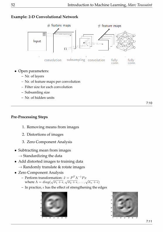
Example: 2-D Convolutional Network
• Open parameters:– Nr. of layers
– Nr. of feature maps per convolution
– Filter size for each convolution
– Subsamling size
– Nr. of hidden units7:10
Pre-Processing Steps
1. Removing means from images
2. Distortions of images
3. Zero Component Analysis
• Subtracting mean from images→ Standardizing the data• Add distorted images to training data→ Randomly translate & rotate images• Zero Component Analysis
– Perform transformation: x = PTΛ−1Pxwhere Λ = diag(
√σ1 + ε,
√σ2 + ε, . . . ,
√σn + ε)
– In practice, ε has the effect of strengthening the edges
7:11
Introduction to Machine Learning, Marc Toussaint 53
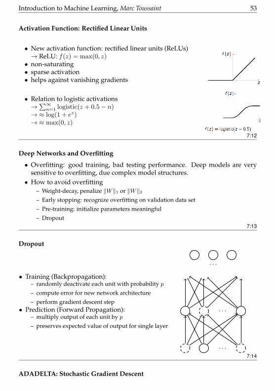
Activation Function: Rectified Linear Units
• New activation function: rectified linear units (ReLUs)→ ReLU: f(z) = max(0, z)• non-saturating• sparse activation• helps against vanishing gradients
• Relation to logistic activations→∑∞n=1 logistic(z + 0.5− n)
→≈ log(1 + ez)→≈ max(0, z)
7:12
Deep Networks and Overfitting
• Overfitting: good training, bad testing performance. Deep models are verysensitive to overfitting, due complex model structures.• How to avoid overfitting
– Weight-decay, penalize ‖W‖1 or ‖W‖2– Early stopping: recognize overfitting on validation data set
– Pre-training: initialize parameters meaningful
– Dropout7:13
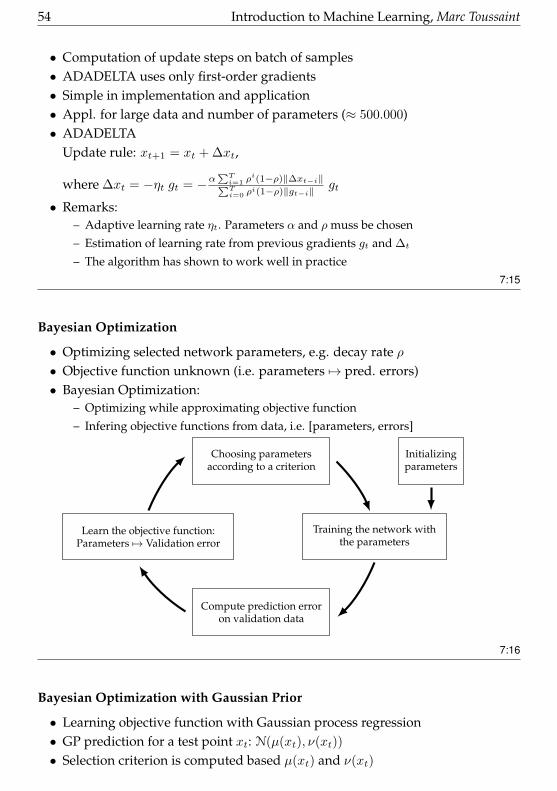
Dropout
• Training (Backpropagation):– randomly deactivate each unit with probability p
– compute error for new network architecture
– perform gradient descent step• Prediction (Forward Propagation):
– multiply output of each unit by p
– preserves expected value of output for single layer
. . .
. . .
. . .
7:14
ADADELTA: Stochastic Gradient Descent
54 Introduction to Machine Learning, Marc Toussaint
• Computation of update steps on batch of samples• ADADELTA uses only first-order gradients• Simple in implementation and application• Appl. for large data and number of parameters (≈ 500.000)• ADADELTA
Update rule: xt+1 = xt + ∆xt,
where ∆xt = −ηt gt = −α∑Ti=1 ρ
i(1−ρ)‖∆xt−i‖∑Ti=0 ρ
i(1−ρ)‖gt−i‖gt
• Remarks:– Adaptive learning rate ηt. Parameters α and ρ muss be chosen
– Estimation of learning rate from previous gradients gt and ∆t
– The algorithm has shown to work well in practice7:15
Bayesian Optimization
• Optimizing selected network parameters, e.g. decay rate ρ• Objective function unknown (i.e. parameters 7→ pred. errors)• Bayesian Optimization:
– Optimizing while approximating objective function
– Infering objective functions from data, i.e. [parameters, errors]
Initializingparameters
Training the network withthe parameters
Compute prediction erroron validation data
Learn the objective function:Parameters 7→ Validation error
Choosing parametersaccording to a criterion
7:16
Bayesian Optimization with Gaussian Prior
• Learning objective function with Gaussian process regression• GP prediction for a test point xt: N(µ(xt), ν(xt))
• Selection criterion is computed based µ(xt) and ν(xt)
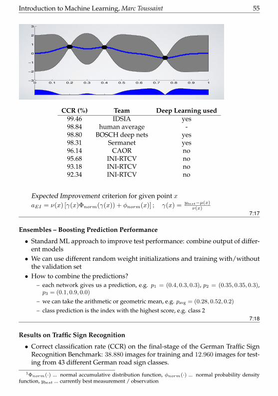
Introduction to Machine Learning, Marc Toussaint 55Expected Improvement
0 0.1 0.2 0.3 0.4 0.5 0.6 0.7 0.8 0.9 1−3
−2
−1
0
1
2
3
CCR (%) Team Deep Learning used99.46 IDSIA yes98.84 human average -98.80 BOSCH deep nets yes98.31 Sermanet yes96.14 CAOR no95.68 INI-RTCV no93.18 INI-RTCV no92.34 INI-RTCV no
Expected Improvement criterion for given point xaEI = ν(x) [γ(x)Φnorm(γ(x)) + φnorm(x)] ; γ(x) = ybest−µ(x)
ν(x)7:17
Ensembles – Boosting Prediction Performance
• Standard ML approach to improve test performance: combine output of differ-ent models• We can use different random weight initializations and training with/without
the validation set• How to combine the predictions?
– each network gives us a prediction, e.g. p1 = (0.4, 0.3, 0.3), p2 = (0.35, 0.35, 0.3),p3 = (0.1, 0.9, 0.0)
– we can take the arithmetic or geometric mean, e.g. pavg = (0.28, 0.52, 0.2)
– class prediction is the index with the highest score, e.g. class 27:18
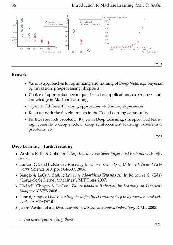
Results on Traffic Sign Recognition
• Correct classification rate (CCR) on the final-stage of the German Traffic SignRecognition Benchmark: 38.880 images for training and 12.960 images for test-ing from 43 different German road sign classes.
1Φnorm(·) ... normal accumulative distribution function, φnorm(·) ... normal probability densityfunction, ybest ... currently best measurement / observation
56 Introduction to Machine Learning, Marc Toussaint
Year
ErrorRate
* only 10 best results plotted
2010 2011 2012 2013* 2014*
60%
40%
26.2%
20%16.4%
10%
traditional
involves deep learning
Year
Error
Score
2013 2014
100
90
80
70
60
traditional
involves deep learning
Year
# DL Publications Google Scholar
* as of October 14, 2014
2000 2005 2010 2014*
1400
1200
1000
800
600
400
200
7:19
Remarks
• Various approaches for optimizing and training of Deep Nets, e.g. Bayesianoptimization, pre-processing, dropouts ...
• Choice of appropriate techniques based on applications, experiences andknowledge in Machine Learning
• Try-out of different training approaches→ Gaining experiences
• Keep up with the developments in the Deep Learning community
• Further research problems: Bayesian Deep Learning, unsupervised learn-ing, generative deep models, deep reinforcement learning, adversarialproblems, etc.
7:20
Deep Learning – further reading
• Weston, Ratle & Collobert: Deep Learning via Semi-Supervised Embedding, ICML2008.• Hinton & Salakhutdinov: Reducing the Dimensionality of Data with Neural Net-
works, Science 313, pp. 504-507, 2006.• Bengio & LeCun: Scaling Learning Algorithms Towards AI. In Bottou et al. (Eds)
“Large-Scale Kernel Machines”, MIT Press 2007.• Hadsell, Chopra & LeCun: Dimensionality Reduction by Learning an Invariant
Mapping, CVPR 2006.• Glorot, Bengio: Understanding the difficulty of training deep feedforward neural net-
works, AISTATS’10.• Jason Weston et al.: Deep Learning via Semi-SupervisedEmbedding, ICML 2008.
... and newer papers citing those7:21
Introduction to Machine Learning, Marc Toussaint 57
8 The Breadth of MLLocal Models & Boosting
Local & Lazy learning
• Idea of local (or “lazy”) learning:Do not try to build one global model f(x) from the data. Instead, whenever wehave a query point x∗, we build a specific local model in the neighborhood ofx∗.
• Typical approach:– Given a query point x∗, find all kNN in the data D = (xi, yi)Ni=1
– Fit a local model fx∗ only to these kNNs, perhaps weighted– Use the local model fx∗ to predict x∗ 7→ y0
• Weighted local least squares:
Llocal(β, x∗) =∑ni=1K(x∗, xi)(yi − f(xi))
2 + λ||β||2
where K(x∗, x) is called smoothing kernel. The optimum is:
β = (X>WX + λI)-1X>Wy , W = diag(K(x∗, x1:n))
8:1
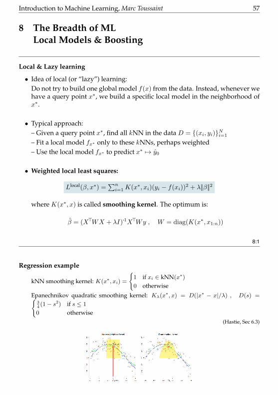
Regression example
kNN smoothing kernel: K(x∗, xi) =
1 if xi ∈ kNN(x∗)
0 otherwise
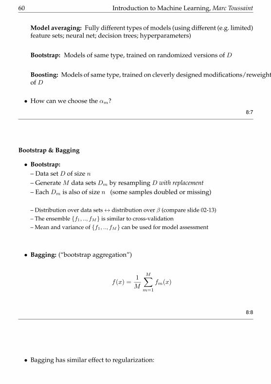
Epanechnikov quadratic smoothing kernel: Kλ(x∗, x) = D(|x∗ − x|/λ) , D(s) =34(1− s2) if s ≤ 1
0 otherwise(Hastie, Sec 6.3)

58 Introduction to Machine Learning, Marc Toussaint
8:2
Smoothing Kernels
from Wikipedia
8:3
kd-trees
• For local & lazy learning it is essential to efficiently retrieve the kNN
Problem: Given data X , a query x∗, identify the kNNs of x∗ in X .
• Linear time (stepping through all of X) is far too slow.
A kd-tree pre-structures the data into a binary tree, allowing O(log n) retrievalof kNNs.
8:4
Introduction to Machine Learning, Marc Toussaint 59
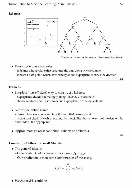
kd-trees
(There are “typos” in this figure... Exercise to find them.)
• Every node plays two roles:– it defines a hyperplane that separates the data along one coordinate– it hosts a data point, which lives exactly on the hyperplane (defines the division)
8:5
kd-trees
• Simplest (non-efficient) way to construct a kd-tree:– hyperplanes divide alternatingly along 1st, 2nd, ... coordinate– choose random point, use it to define hyperplane, divide data, iterate
• Nearest neighbor search:– descent to a leave node and take this as initial nearest point– ascent and check at each branching the possibility that a nearer point exists on theother side of the hyperplane
• Approximate Nearest Neighbor (libann on Debian..)8:6
Combining Different (Local) Models
• The general idea is:– Given data D, let us learn various models f1, .., fM
– Our prediction is then some combination of these, e.g.
f(x) =
M∑m=1
αmfm(x)
• Various models could be:
60 Introduction to Machine Learning, Marc Toussaint
Model averaging: Fully different types of models (using different (e.g. limited)feature sets; neural net; decision trees; hyperparameters)
Bootstrap: Models of same type, trained on randomized versions of D
Boosting: Models of same type, trained on cleverly designed modifications/reweightingsof D
• How can we choose the αm?
8:7
Bootstrap & Bagging
• Bootstrap:– Data set D of size n– Generate M data sets Dm by resampling D with replacement– Each Dm is also of size n (some samples doubled or missing)
– Distribution over data sets↔ distribution over β (compare slide 02-13)– The ensemble f1, .., fM is similar to cross-validation– Mean and variance of f1, .., fM can be used for model assessment
• Bagging: (“bootstrap aggregation”)
f(x) =1
M
M∑m=1
fm(x)
8:8
• Bagging has similar effect to regularization:
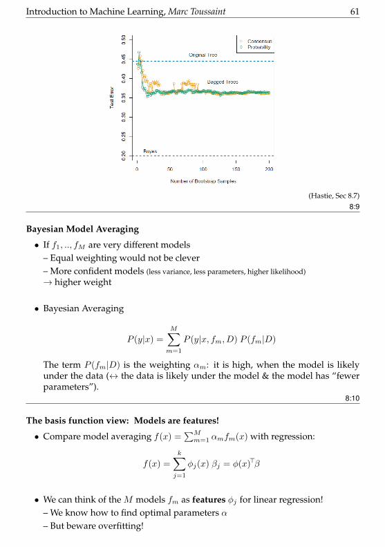
Introduction to Machine Learning, Marc Toussaint 61
(Hastie, Sec 8.7)8:9
Bayesian Model Averaging
• If f1, .., fM are very different models– Equal weighting would not be clever– More confident models (less variance, less parameters, higher likelihood)→ higher weight
• Bayesian Averaging
P (y|x) =
M∑m=1
P (y|x, fm, D) P (fm|D)
The term P (fm|D) is the weighting αm: it is high, when the model is likelyunder the data (↔ the data is likely under the model & the model has “fewerparameters”).
8:10
The basis function view: Models are features!
• Compare model averaging f(x) =∑Mm=1 αmfm(x) with regression:
f(x) =
k∑j=1
φj(x) βj = φ(x)>β
• We can think of the M models fm as features φj for linear regression!– We know how to find optimal parameters α– But beware overfitting!
62 Introduction to Machine Learning, Marc Toussaint
8:11
Boosting
• In Bagging and Model Averaging, the models are trained on the “same data”(unbiased randomized versions of the same data)
• Boosting tries to be cleverer:– It adapts the data for each learner– It assigns each learner a differently weighted version of the data
• With this, boosing can– Combine many “weak” classifiers to produce a powerful “committee”– A weak learner only needs to be somewhat better than random
8:12
AdaBoost
(Freund & Schapire, 1997)(classical Algo; use Gradient Boosting instead in practice)
• Binary classification problem with data D = (xi, yi)ni=1, yi ∈ −1,+1• We know how to train discriminative functions f(x); let
G(x) = sign f(x) ∈ −1,+1
• We will train a sequence of classificers G1, .., GM , each on differently weighteddata, to yield a classifier
G(x) = sign
M∑m=1
αmGm(x)
8:13
Introduction to Machine Learning, Marc Toussaint 63
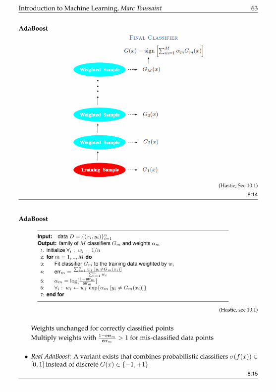
AdaBoost
(Hastie, Sec 10.1)
8:14
AdaBoost
Input: data D = (xi, yi)ni=1
Output: family of M classifiers Gm and weights αm1: initialize ∀i : wi = 1/n
2: for m = 1, ..,M do3: Fit classifier Gm to the training data weighted by wi4: errm =
∑ni=1 wi [yi 6=Gm(xi)]∑n
i=1 wi
5: αm = log[ 1−errmerrm
]
6: ∀i : wi ← wi expαm [yi 6= Gm(xi)]7: end for
(Hastie, sec 10.1)
Weights unchanged for correctly classified pointsMultiply weights with 1−errm
errm> 1 for mis-classified data points
• Real AdaBoost: A variant exists that combines probabilistic classifiers σ(f(x)) ∈[0, 1] instead of discrete G(x) ∈ −1,+1
8:15

64 Introduction to Machine Learning, Marc Toussaint
The basis function view
• In AdaBoost, each model Gm depends on the data weights wmWe could write this as
f(x) =
M∑m=1
αmfm(x,wm)
The “features” fm(x,wm) now have additional parameters wmWe’d like to optimize
minα,w1,..,wM
L(f)
w.r.t. α and all the feature parameters wm.
• In general this is hard.But assuming αm and wm fixed, optimizing for αm and wm is efficient.
• AdaBoost does exactly this, choosing wm so that the “feature” fm will bestreduce the loss (cf. PLS)(Literally, AdaBoost uses exponential loss or neg-log-likelihood; Hastie sec 10.4 & 10.5)
8:16
Gradient Boosting
• AdaBoost generates a series of basis functions by using different data weight-ings wm depending on so-far classification errors• We can also generate a series of basis functions fm by fitting them to the gradi-
ent of the so-far loss8:17
Gradient Boosting
• Assume we want to miminize some loss function
minfL(f) =
n∑i=1
L(yi, f(xi))
We can solve this using gradient descent
f∗ = f0 + α1∂L(f0)
∂f︸ ︷︷ ︸≈f1
+α2∂L(f0 + α1f1)
∂f︸ ︷︷ ︸≈f2
+α3∂L(f0 + α1f1 + α2f2)
∂f︸ ︷︷ ︸≈f3
+ · · ·
– Each fm aproximates the so-far loss gradient– We use linear regression to choose αm (instead of line search)
Introduction to Machine Learning, Marc Toussaint 65
• More intuitively: ∂L(f)∂f “points into the direction of the error/redisual of f”. It
shows how f could be improved.
Gradient boosting uses the next lerner fk ≈ ∂L(fso far)∂f to approximate how f can
be improved.Optimizing α’s does the improvement.
8:18
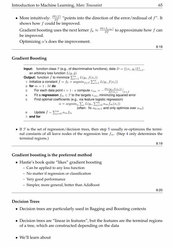
Gradient Boosting
Input: function class F (e.g., of discriminative functions), data D = (xi, yi)ni=1,an arbitrary loss function L(y, y)
Output: function f to minimize∑ni=1 L(yi, f(xi))
1: Initialize a constant f = f0 = argminf∈F∑ni=1 L(yi, f(xi))
2: for m = 1 : M do3: For each data point i = 1 : n compute rim = − ∂L(yi,f(xi))
∂f(xi)
∣∣f=f
4: Fit a regression fm ∈ F to the targets rim, minimizing squared error5: Find optimal coefficients (e.g., via feature logistic regression)
α = argminα∑i L(yi,
∑mj=0 αmfm(xi))
(often: fix α0:m-1 and only optimize over αm)6: Update f =
∑mj=0 αmfm
7: end for
• If F is the set of regression/decision trees, then step 5 usually re-optimizes the termi-nal constants of all leave nodes of the regression tree fm. (Step 4 only determines theterminal regions.)
8:19
Gradient boosting is the preferred method
• Hastie’s book quite “likes” gradient boosting– Can be applied to any loss function
– No matter if regression or classification
– Very good performance
– Simpler, more general, better than AdaBoost8:20
Decision Trees
• Decision trees are particularly used in Bagging and Boosting contexts
• Decision trees are “linear in features”, but the features are the terminal regionsof a tree, which are constructed depending on the data
• We’ll learn about

66 Introduction to Machine Learning, Marc Toussaint
– Boosted decision trees & stumps– Random Forests
8:21
Decision Trees
• We describe CART (classification and regression tree)• Decision trees are linear in features:
f(x) =
k∑j=1
cj [x ∈ Rj ]
where Rj are disjoint rectangular regions and cj the constant prediction in aregion• The regions are defined by a binary decision tree
8:22
Growing the decision tree
• The constants are the region averages cj =∑i yi [xi∈Rj ]∑i[xi∈Rj ]
• Each split xa > t is defined by a choice of input dimension a ∈ 1, .., d and athreshold t• Given a yet unsplit region Rj , we split it by choosing
mina,t
[minc1
∑i:xi∈Rj∧xa≤t
(yi − c1)2 + minc2
∑i:xi∈Rj∧xa>t
(yi − c2)2]
– Finding the threshold t is really quick (slide along)
– We do this for every input dimension a8:23
Deciding on the depth (if not pre-fixed)
Introduction to Machine Learning, Marc Toussaint 67
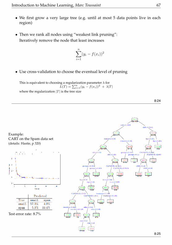
• We first grow a very large tree (e.g. until at most 5 data points live in eachregion)
• Then we rank all nodes using “weakest link pruning”:Iteratively remove the node that least increases
n∑i=1
(yi − f(xi))2
• Use cross-validation to choose the eventual level of pruning
This is equivalent to choosing a regularization parameter λ forL(T ) =
∑ni=1(yi − f(xi))
2 + λ|T |where the regularization |T | is the tree size
8:24
Example:CART on the Spam data set(details: Hastie, p 320)
Test error rate: 8.7%
8:25
68 Introduction to Machine Learning, Marc Toussaint
Boosting trees & stumps
• A decision stump is a decision tree with fixed depth 1 (just one split)
• Gradient boosting of decision trees (of fixed depth J) and stumps is very effec-tive
Test error rates on Spam data set:full decision tree 8.7%
boosted decision stumps 4.7%boosted decision trees with J = 5 4.5%
8:26
Random Forests: Bootstrapping & randomized splits
• Recall that Bagging averages models f1, .., fM where each fm was trained on abootstrap resample Dm of the data DThis randomizes the models and avoids over-generalization
• Random Forests do Bagging, but additionally randomize the trees:– When growing a new split, choose the input dimension a only from a random subsetm features
– m is often very small; even m = 1 or m = 3
• Random Forests are the prime example for “creating many randomized weaklearners from the same data D”
8:27
Introduction to Machine Learning, Marc Toussaint 69
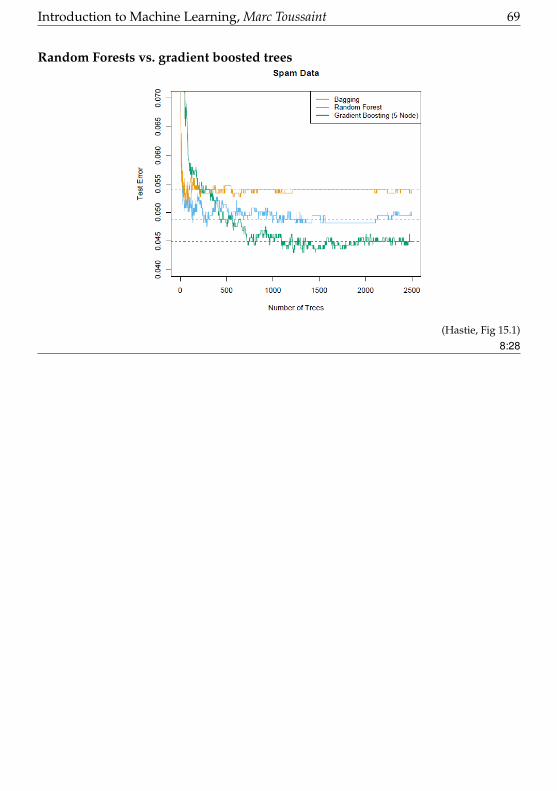
Random Forests vs. gradient boosted trees
(Hastie, Fig 15.1)8:28
70 Introduction to Machine Learning, Marc Toussaint
9 The Breadth of MLCRF & Recap: Probability
Structured Output & Structured Input
• Regression:
Rn → R
• Structured Output:
Rn → binary class label 0, 1Rn → integer class label 1, 2, ..,MRn → sequence labelling y1:T
Rn → image labelling y1:W,1:H
Rn → graph labelling y1:N
• Structured Input:
relational database→ Rlabelled graph/sequence→ R
9:1
Examples for Structured Output
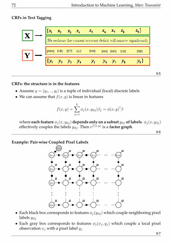
• Text taggingX = sentenceY = tagging of each wordhttp://sourceforge.net/projects/crftagger
• Image segmentationX = imageY = labelling of each pixelhttp://scholar.google.com/scholar?cluster=13447702299042713582
• Depth estimationX = single imageY = depth maphttp://make3d.cs.cornell.edu/
9:2
Introduction to Machine Learning, Marc Toussaint 71
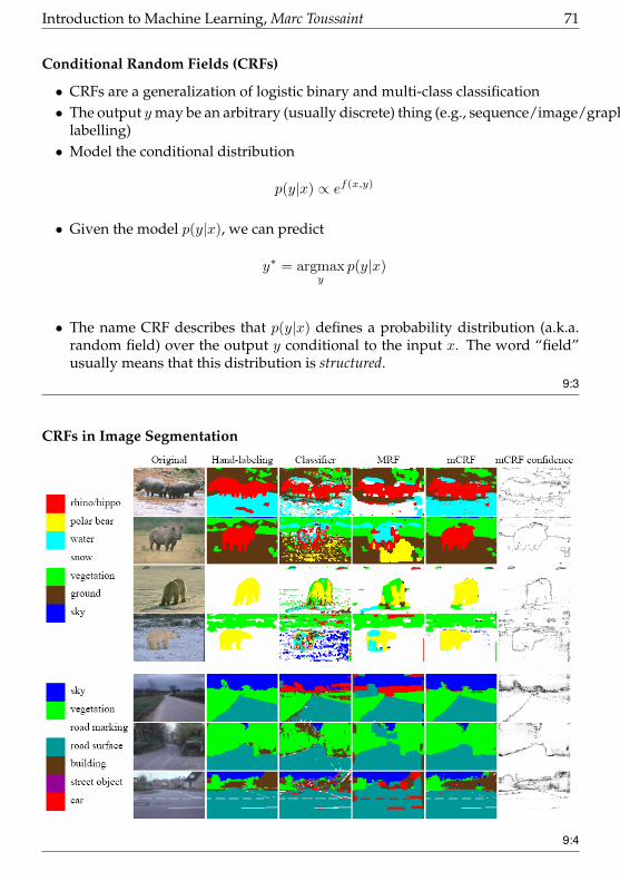
Conditional Random Fields (CRFs)
• CRFs are a generalization of logistic binary and multi-class classification• The output y may be an arbitrary (usually discrete) thing (e.g., sequence/image/graph-
labelling)• Model the conditional distribution
p(y|x) ∝ ef(x,y)
• Given the model p(y|x), we can predict
y∗ = argmaxy
p(y|x)
• The name CRF describes that p(y|x) defines a probability distribution (a.k.a.random field) over the output y conditional to the input x. The word “field”usually means that this distribution is structured.
9:3
CRFs in Image Segmentation
9:4
72 Introduction to Machine Learning, Marc Toussaint
CRFs in Text Tagging
9:5
CRFs: the structure is in the features
• Assume y = (y1, .., yl) is a tuple of individual (local) discrete labels• We can assume that f(x, y) is linear in features
f(x, y) =
k∑j=1
φj(x, y∂j)βj = φ(x, y)>β
where each feature φj(x, y∂j) depends only on a subset y∂j of labels. φj(x, y∂j)effectively couples the labels y∂j . Then ef(x,y) is a factor graph.
9:6
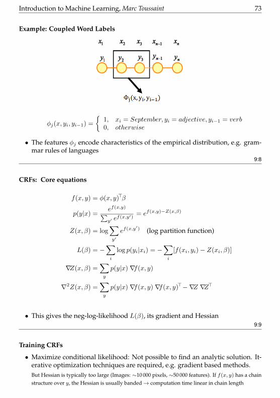
Example: Pair-wise Coupled Pixel Labels
y31
yH1
y11 y12 y13 y14 y1W
y21
x11
• Each black box corresponds to features φj(y∂j) which couple neighboring pixellabels y∂j• Each gray box corresponds to features φj(xj , yj) which couple a local pixel
observation xj with a pixel label yj9:7
Introduction to Machine Learning, Marc Toussaint 73
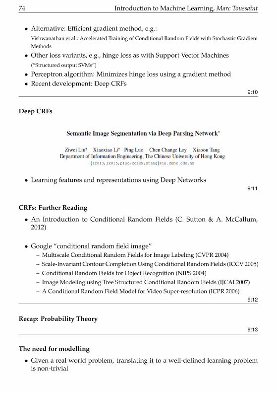
Example: Coupled Word Labels
φj(x, yi, yi−1) =
1, xi = September, yi = adjective, yi−1 = verb0, otherwise
• The features φj encode characteristics of the empirical distribution, e.g. gram-mar rules of languages
9:8
CRFs: Core equations
f(x, y) = φ(x, y)>β
p(y|x) =ef(x,y)∑y′ e
f(x,y′)= ef(x,y)−Z(x,β)
Z(x, β) = log∑y′
ef(x,y′) (log partition function)
L(β) = −∑i
log p(yi|xi) = −∑i
[f(xi, yi)− Z(xi, β)]
∇Z(x, β) =∑y
p(y|x)∇f(x, y)
∇2Z(x, β) =∑y
p(y|x)∇f(x, y)∇f(x, y)>−∇Z ∇Z>
• This gives the neg-log-likelihood L(β), its gradient and Hessian9:9
Training CRFs
• Maximize conditional likelihood: Not possible to find an analytic solution. It-erative optimization techniques are required, e.g. gradient based methods.But Hessian is typically too large (Images: ∼10 000 pixels, ∼50 000 features). If f(x, y) has a chainstructure over y, the Hessian is usually banded→ computation time linear in chain length
74 Introduction to Machine Learning, Marc Toussaint
• Alternative: Efficient gradient method, e.g.:Vishwanathan et al.: Accelerated Training of Conditional Random Fields with Stochastic GradientMethods
• Other loss variants, e.g., hinge loss as with Support Vector Machines(“Structured output SVMs”)
• Perceptron algorithm: Minimizes hinge loss using a gradient method• Recent development: Deep CRFs
9:10
Deep CRFs
• Learning features and representations using Deep Networks9:11
CRFs: Further Reading
• An Introduction to Conditional Random Fields (C. Sutton & A. McCallum,2012)
• Google “conditional random field image”– Multiscale Conditional Random Fields for Image Labeling (CVPR 2004)
– Scale-Invariant Contour Completion Using Conditional Random Fields (ICCV 2005)
– Conditional Random Fields for Object Recognition (NIPS 2004)
– Image Modeling using Tree Structured Conditional Random Fields (IJCAI 2007)
– A Conditional Random Field Model for Video Super-resolution (ICPR 2006)9:12
Recap: Probability Theory
9:13
The need for modelling
• Given a real world problem, translating it to a well-defined learning problemis non-trivial
Introduction to Machine Learning, Marc Toussaint 75
• The “framework” of plain regression/classification is restricted: input x, out-put y.
• Graphical models (probabilstic models with multiple random variables and de-pendencies) are a more general framework for modelling “problems”; regres-sion & classification become a special case; Reinforcement Learning, decisionmaking, unsupervised learning, but also language processing, image segmen-tation, can be represented.
9:14
Outline
• Basic definitions– Random variables
– joint, conditional, marginal distribution
– Bayes’ theorem
• Examples for Bayes• Probability distributions [skipped, only Gauss]
– Binomial; Beta
– Multinomial; Dirichlet
– Conjugate priors
– Gauss; Wichart
– Student-t, Dirak, Particles
• Monte Carlo, MCMC [skipped]These are generic slides on probabilities I use throughout my lecture. Only parts aremandatory for the AI course.
9:15
Thomas Bayes (1702-–1761)
“Essay Towards Solving aProblem in the Doctrine ofChances”
• Addresses problem of inverse probabilities:Knowing the conditional probability of B given A, what is the conditional prob-

76 Introduction to Machine Learning, Marc Toussaint
ability of A given B?
• Example:40% Bavarians speak dialect, only 1% of non-Bavarians speak (Bav.) dialectGiven a random German that speaks non-dialect, is he Bavarian?(15% of Germans are Bavarian)
9:16
Inference
• “Inference” = Given some pieces of information (prior, observed variabes) whatis the implication (the implied information, the posterior) on a non-observedvariable
• Decision-Making and Learning as Inference:– given pieces of information: about the world/game, collected data, assumed
model class, prior over model parameters
– make decisions about actions, classifier, model parameters, etc9:17
Probability Theory
• Why do we need probabilities?– Obvious: to express inherent stochasticity of the world (data)
• But beyond this: (also in a “deterministic world”):– lack of knowledge!
– hidden (latent) variables
– expressing uncertainty– expressing information (and lack of information)
• Probability Theory: an information calculus9:18
Probability: Frequentist and Bayesian
• Frequentist probabilities are defined in the limit of an infinite number of trialsExample: “The probability of a particular coin landing heads up is 0.43”
• Bayesian (subjective) probabilities quantify degrees of beliefExample: “The probability of rain tomorrow is 0.3” – not possible to repeat “tomorrow”
9:19
Introduction to Machine Learning, Marc Toussaint 77
Basic definitions
9:20
Probabilities & Random Variables
• For a random variable X with discrete domain dom(X) = Ω we write:∀x∈Ω : 0 ≤ P (X=x) ≤ 1∑x∈Ω P (X=x) = 1
Example: A dice can take values Ω = 1, .., 6.X is the random variable of a dice throw.P (X=1) ∈ [0, 1] is the probability that X takes value 1.
• A bit more formally: a random variable is a map from a measureable space to a domain(sample space) and thereby introduces a probability measure on the domain (“assigns aprobability to each possible value”)
9:21
Probabilty Distributions
• P (X=1) ∈ R denotes a specific probabilityP (X) denotes the probability distribution (function over Ω)
Example: A dice can take values Ω = 1, 2, 3, 4, 5, 6.By P (X) we discribe the full distribution over possible values 1, .., 6. These are 6numbers that sum to one, usually stored in a table, e.g.: [ 1
6, 16, 16, 16, 16, 16]
• In implementations we typically represent distributions over discrete randomvariables as tables (arrays) of numbers
• Notation for summing over a RV:In equation we often need to sum over RVs. We then write∑
X P (X) · · ·as shorthand for the explicit notation
∑x∈dom(X) P (X=x) · · ·
9:22
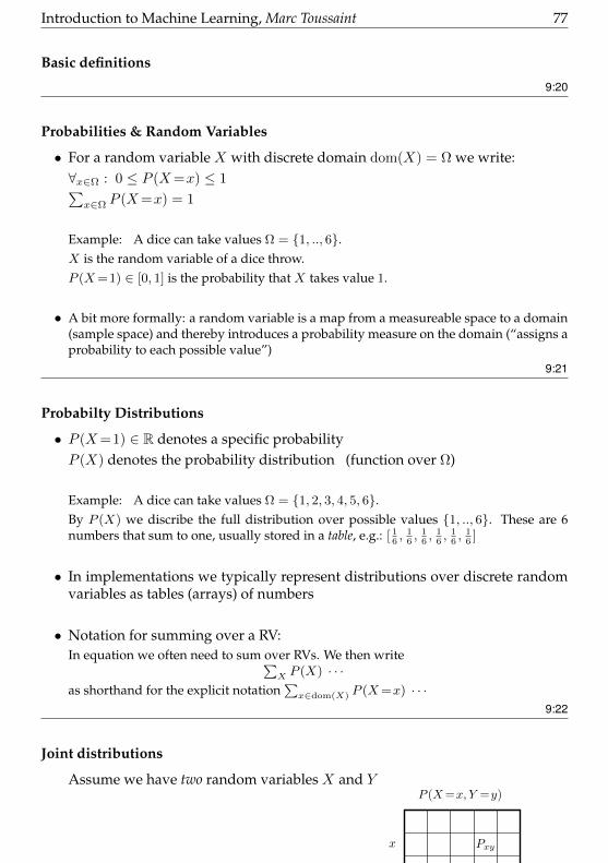
Joint distributions
Assume we have two random variables X and Y

78 Introduction to Machine Learning, Marc Toussaint
• Definitions:Joint: P (X,Y )
Marginal: P (X) =∑Y P (X,Y )
Conditional: P (X|Y ) = P (X,Y )P (Y )
The conditional is normalized: ∀Y :∑X P (X|Y ) = 1
• X is independent of Y iff: P (X|Y ) = P (X)
(table thinking: all columns of P (X|Y ) are equal)9:23
Joint distributions
joint: P (X,Y )
marginal: P (X) =∑Y P (X,Y )
conditional: P (X|Y ) = P (X,Y )P (Y )
• Implications of these definitions:Product rule: P (X,Y ) = P (X|Y ) P (Y ) = P (Y |X) P (X)
Bayes’ Theorem: P (X|Y ) = P (Y |X) P (X)P (Y )
9:24
Bayes’ Theorem
P (X|Y ) =P (Y |X) P (X)
P (Y )
posterior =likelihood · prior
normalization9:25
Multiple RVs:
• Analogously for n random variables X1:n (stored as a rank n tensor)Joint: P (X1:n)
Marginal: P (X1) =∑X2:n
P (X1:n),
Conditional: P (X1|X2:n) = P (X1:n)P (X2:n)
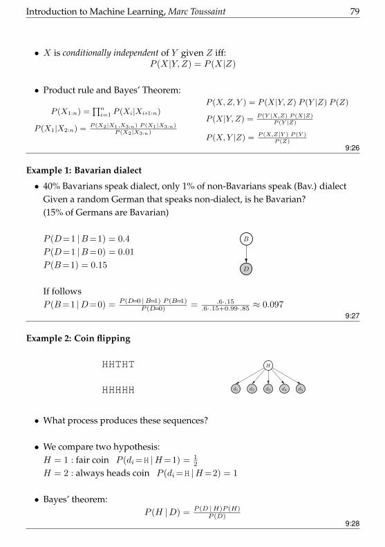
Introduction to Machine Learning, Marc Toussaint 79
• X is conditionally independent of Y given Z iff:P (X|Y, Z) = P (X|Z)
• Product rule and Bayes’ Theorem:
P (X1:n) =∏ni=1 P (Xi|Xi+1:n)
P (X1|X2:n) = P (X2|X1,X3:n) P (X1|X3:n)P (X2|X3:n)
P (X,Z, Y ) = P (X|Y,Z) P (Y |Z) P (Z)
P (X|Y,Z) = P (Y |X,Z) P (X|Z)P (Y |Z)
P (X,Y |Z) = P (X,Z|Y ) P (Y )P (Z)
9:26
Example 1: Bavarian dialect
• 40% Bavarians speak dialect, only 1% of non-Bavarians speak (Bav.) dialectGiven a random German that speaks non-dialect, is he Bavarian?(15% of Germans are Bavarian)
P (D=1 |B=1) = 0.4
P (D=1 |B=0) = 0.01
P (B=1) = 0.15
If follows
D
B
P (B=1 |D=0) = P (D=0 |B=1) P (B=1)P (D=0) = .6·.15
.6·.15+0.99·.85 ≈ 0.0979:27
Example 2: Coin flipping
HHTHT
HHHHH
H
d1 d2 d3 d4 d5
• What process produces these sequences?
• We compare two hypothesis:H = 1 : fair coin P (di=H |H=1) = 1
2
H = 2 : always heads coin P (di=H |H=2) = 1
• Bayes’ theorem:P (H |D) = P (D |H)P (H)
P (D)9:28
80 Introduction to Machine Learning, Marc Toussaint
Coin flipping
D = HHTHT
P (D |H=1) = 1/25 P (H=1) = 9991000
P (D |H=2) = 0 P (H=2) = 11000
P (H=1 |D)
P (H=2 |D)=P (D |H=1)
P (D |H=2)
P (H=1)
P (H=2)=
1/32
0
999
1=∞
9:29
Coin flipping
D = HHHHH
P (D |H=1) = 1/25 P (H=1) = 9991000
P (D |H=2) = 1 P (H=2) = 11000
P (H=1 |D)
P (H=2 |D)=P (D |H=1)
P (D |H=2)
P (H=1)
P (H=2)=
1/32
1
999
1≈ 30
9:30
Coin flipping
D = HHHHHHHHHH
P (D |H=1) = 1/210 P (H=1) = 9991000
P (D |H=2) = 1 P (H=2) = 11000
P (H=1 |D)
P (H=2 |D)=P (D |H=1)
P (D |H=2)
P (H=1)
P (H=2)=
1/1024
1
999
1≈ 1
9:31
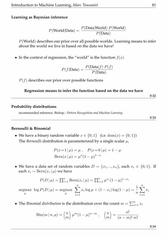
Introduction to Machine Learning, Marc Toussaint 81
Learning as Bayesian inference
P (World|Data) =P (Data|World) P (World)
P (Data)
P (World) describes our prior over all possible worlds. Learning means to inferabout the world we live in based on the data we have!
• In the context of regression, the “world” is the function f(x)
P (f |Data) =P (Data|f) P (f)
P (Data)
P (f) describes our prior over possible functions
Regression means to infer the function based on the data we have9:32
Probability distributionsrecommended reference: Bishop.: Pattern Recognition and Machine Learning
9:33
Bernoulli & Binomial
• We have a binary random variable x ∈ 0, 1 (i.e. dom(x) = 0, 1)The Bernoulli distribution is parameterized by a single scalar µ,
P (x=1 |µ) = µ , P (x=0 |µ) = 1− µBern(x |µ) = µx(1− µ)1−x
• We have a data set of random variables D = x1, .., xn, each xi ∈ 0, 1. Ifeach xi ∼ Bern(xi |µ) we have
P (D |µ) =∏ni=1 Bern(xi |µ) =
∏ni=1 µ
xi(1− µ)1−xi
argmaxµ
logP (D |µ) = argmaxµ
n∑i=1
xi logµ+ (1− xi) log(1− µ) =1
n
n∑i=1
xi
• The Binomial distribution is the distribution over the count m =∑ni=1 xi
Bin(m |n, µ) =nm
µm(1− µ)n−m ,nm
=n!
(n−m)! m!
9:34
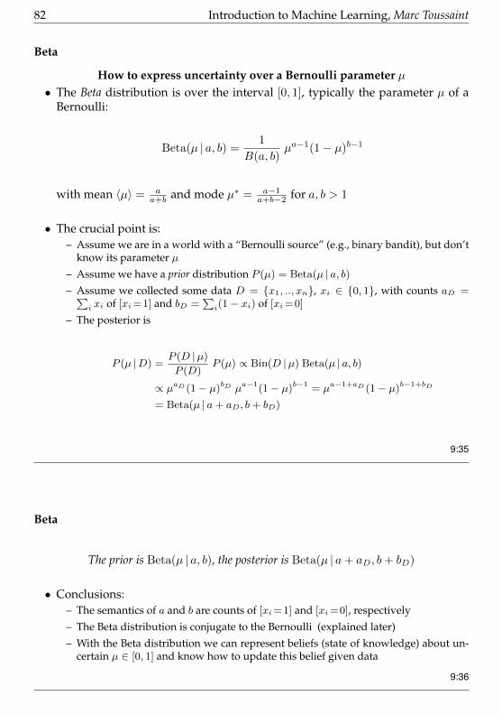
82 Introduction to Machine Learning, Marc Toussaint
Beta
How to express uncertainty over a Bernoulli parameter µ• The Beta distribution is over the interval [0, 1], typically the parameter µ of a
Bernoulli:
Beta(µ | a, b) =1
B(a, b)µa−1(1− µ)b−1
with mean 〈µ〉 = aa+b and mode µ∗ = a−1
a+b−2 for a, b > 1
• The crucial point is:– Assume we are in a world with a “Bernoulli source” (e.g., binary bandit), but don’t
know its parameter µ
– Assume we have a prior distribution P (µ) = Beta(µ | a, b)– Assume we collected some data D = x1, .., xn, xi ∈ 0, 1, with counts aD =∑
i xi of [xi=1] and bD =∑i(1− xi) of [xi=0]
– The posterior is
P (µ |D) =P (D |µ)
P (D)P (µ) ∝ Bin(D |µ) Beta(µ | a, b)
∝ µaD (1− µ)bD µa−1(1− µ)b−1 = µa−1+aD (1− µ)b−1+bD
= Beta(µ | a+ aD, b+ bD)
9:35
Beta
The prior is Beta(µ | a, b), the posterior is Beta(µ | a+ aD, b+ bD)
• Conclusions:– The semantics of a and b are counts of [xi=1] and [xi=0], respectively
– The Beta distribution is conjugate to the Bernoulli (explained later)
– With the Beta distribution we can represent beliefs (state of knowledge) about un-certain µ ∈ [0, 1] and know how to update this belief given data
9:36
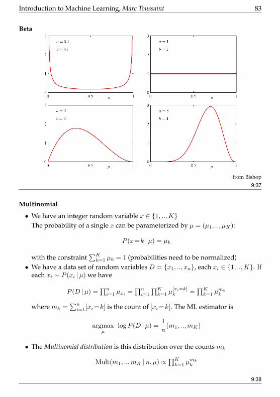
Introduction to Machine Learning, Marc Toussaint 83
Beta
from Bishop
9:37
Multinomial
• We have an integer random variable x ∈ 1, ..,KThe probability of a single x can be parameterized by µ = (µ1, .., µK):
P (x=k |µ) = µk
with the constraint∑Kk=1 µk = 1 (probabilities need to be normalized)
• We have a data set of random variables D = x1, .., xn, each xi ∈ 1, ..,K. Ifeach xi ∼ P (xi |µ) we have
P (D |µ) =∏ni=1 µxi =
∏ni=1
∏Kk=1 µ
[xi=k]k =
∏Kk=1 µ
mkk
where mk =∑ni=1[xi=k] is the count of [xi=k]. The ML estimator is
argmaxµ
logP (D |µ) =1
n(m1, ..,mK)
• The Multinomial distribution is this distribution over the counts mk
Mult(m1, ..,mK |n, µ) ∝∏Kk=1 µ
mkk
9:38

84 Introduction to Machine Learning, Marc Toussaint
Dirichlet
How to express uncertainty over a Multinomial parameter µ• The Dirichlet distribution is over the K-simplex, that is, over µ1, .., µK ∈ [0, 1]
subject to the constraint∑Kk=1 µk = 1:
Dir(µ |α) ∝∏Kk=1 µ
αk−1k
It is parameterized by α = (α1, .., αK), has mean 〈µi〉 = αi∑jαj
and mode µ∗i =αi−1∑jαj−K
for ai > 1.
• The crucial point is:– Assume we are in a world with a “Multinomial source” (e.g., an integer bandit), but
don’t know its parameter µ
– Assume we have a prior distribution P (µ) = Dir(µ |α)
– Assume we collected some data D = x1, .., xn, xi ∈ 1, ..,K, with counts mk =∑i[xi=k]
– The posterior is
P (µ |D) =P (D |µ)
P (D)P (µ) ∝ Mult(D |µ) Dir(µ | a, b)
∝∏Kk=1 µ
mkk
∏Kk=1 µ
αk−1k =
∏Kk=1 µ
αk−1+mkk
= Dir(µ |α+m)
9:39
Dirichlet
The prior is Dir(µ |α), the posterior is Dir(µ |α+m)
• Conclusions:– The semantics of α is the counts of [xi=k]
– The Dirichlet distribution is conjugate to the Multinomial
– With the Dirichlet distribution we can represent beliefs (state of knowledge) aboutuncertain µ of an integer random variable and know how to update this belief givendata
9:40
Dirichlet
Illustrations for α = (0.1, 0.1, 0.1), α = (1, 1, 1) and α = (10, 10, 10):
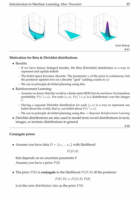
Introduction to Machine Learning, Marc Toussaint 85
from Bishop9:41
Motivation for Beta & Dirichlet distributions
• Bandits:– If we have binary [integer] bandits, the Beta [Dirichlet] distribution is a way to
represent and update beliefs
– The belief space becomes discrete: The parameter α of the prior is continuous, butthe posterior updates live on a discrete “grid” (adding counts to α)
– We can in principle do belief planning using this
• Reinforcement Learning:– Assume we know that the world is a finite-state MDP, but do not know its transition
probability P (s′ | s, a). For each (s, a), P (s′ | s, a) is a distribution over the integers′
– Having a separate Dirichlet distribution for each (s, a) is a way to represent ourbelief about the world, that is, our belief about P (s′ | s, a)
– We can in principle do belief planning using this→ Bayesian Reinforcement Learning
• Dirichlet distributions are also used to model texts (word distributions in text),images, or mixture distributions in general
9:42
Conjugate priors
• Assume you have data D = x1, .., xnwith likelihood
P (D | θ)
that depends on an uncertain parameter θAssume you have a prior P (θ)
• The prior P (θ) is conjugate to the likelihood P (D | θ) iff the posterior
P (θ |D) ∝ P (D | θ) P (θ)
is in the same distribution class as the prior P (θ)
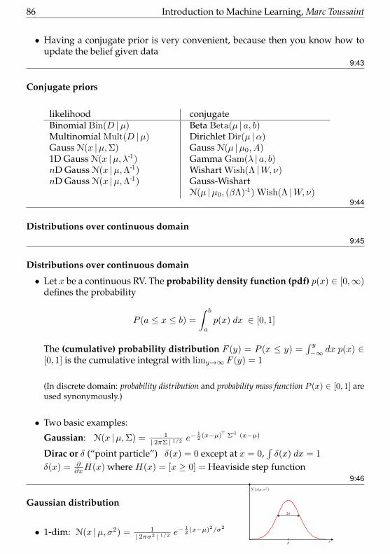
86 Introduction to Machine Learning, Marc Toussaint
• Having a conjugate prior is very convenient, because then you know how toupdate the belief given data
9:43
Conjugate priors
likelihood conjugateBinomial Bin(D |µ) Beta Beta(µ | a, b)Multinomial Mult(D |µ) Dirichlet Dir(µ |α)Gauss N(x |µ,Σ) Gauss N(µ |µ0, A)1D Gauss N(x |µ, λ-1) Gamma Gam(λ | a, b)nD Gauss N(x |µ,Λ-1) Wishart Wish(Λ |W, ν)nD Gauss N(x |µ,Λ-1) Gauss-Wishart
N(µ |µ0, (βΛ)-1) Wish(Λ |W, ν)9:44
Distributions over continuous domain9:45
Distributions over continuous domain
• Let x be a continuous RV. The probability density function (pdf) p(x) ∈ [0,∞)defines the probability
P (a ≤ x ≤ b) =
∫ b
a
p(x) dx ∈ [0, 1]
The (cumulative) probability distribution F (y) = P (x ≤ y) =∫ y−∞ dx p(x) ∈
[0, 1] is the cumulative integral with limy→∞ F (y) = 1
(In discrete domain: probability distribution and probability mass function P (x) ∈ [0, 1] areused synonymously.)
• Two basic examples:
Gaussian: N(x |µ,Σ) = 1| 2πΣ | 1/2 e
− 12 (x−µ)> Σ-1 (x−µ)
Dirac or δ (“point particle”) δ(x) = 0 except at x = 0,∫δ(x) dx = 1
δ(x) = ∂∂xH(x) where H(x) = [x ≥ 0] = Heaviside step function
9:46
Gaussian distribution
• 1-dim: N(x |µ, σ2) = 1| 2πσ2 | 1/2 e
− 12 (x−µ)2/σ2
N (x|µ, σ2)
x
2σ
µ
Introduction to Machine Learning, Marc Toussaint 87
• n-dim Gaussian in normal form:
N(x |µ,Σ) =1
| 2πΣ | 1/2exp−1
2(x− µ)>Σ-1 (x− µ)
with mean µ and covariance matrix Σ. In canonical form:
N[x | a,A] =exp− 1
2a>A-1a
| 2πA-1 | 1/2exp−1
2x>A x+ x>a (1)
with precision matrix A = Σ-1 and coefficient a = Σ-1µ (and mean µ = A-1a).Note: | 2πΣ | = det(2πΣ) = (2π)n det(Σ)
• Gaussian identities: see http://ipvs.informatik.uni-stuttgart.de/mlr/marc/
notes/gaussians.pdf
9:47
Gaussian identities
Symmetry: N(x | a,A) = N(a |x,A) = N(x− a | 0, A)
Product:N(x | a,A) N(x | b,B) = N[x |A-1a+B-1b, A-1 +B-1] N(a | b, A+B)N[x | a,A] N[x | b,B] = N[x | a+ b, A+B] N(A-1a |B-1b, A-1 +B-1)
“Propagation”:∫yN(x | a+ Fy,A) N(y | b,B) dy = N(x | a+ Fb,A+ FBF>)
Transformation:N(Fx+ f | a,A) = 1
|F | N(x | F -1(a− f), F -1AF ->)
Marginal & conditional:
N
(xy
∣∣∣∣ ab , A C
C> B
)= N(x | a,A) ·N(y | b+ C>A-1(x - a), B − C>A-1C)
More Gaussian identities: see http://ipvs.informatik.uni-stuttgart.de/mlr/marc/notes/gaussians.pdf
9:48
Gaussian prior and posterior
• Assume we have data D = x1, .., xn, each xi ∈ Rn, with likelihood
P (D |µ,Σ) =∏iN(xi |µ,Σ)
argmaxµ
P (D |µ,Σ) =1
n
n∑i=1
xi
88 Introduction to Machine Learning, Marc Toussaint
argmaxΣ
P (D |µ,Σ) =1
n
n∑i=1
(xi − µ)(xi − µ)>
• Assume we are initially uncertain about µ (but know Σ). We can express thisuncertainty using again a Gaussian N[µ | a,A]. Given data we have
P (µ |D) ∝ P (D |µ,Σ) P (µ) =∏iN(xi |µ,Σ) N[µ | a,A]
=∏iN[µ |Σ-1xi,Σ
-1] N[µ | a,A] ∝ N[µ |Σ-1∑i xi, nΣ-1 +A]
Note: in the limit A→ 0 (uninformative prior) this becomes
P (µ |D) = N(µ | 1
n
∑i
xi,1
nΣ)
which is consistent with the Maximum Likelihood estimator9:49
Motivation for Gaussian distributions
• Gaussian Bandits• Control theory, Stochastic Optimal Control• State estimation, sensor processing, Gaussian filtering (Kalman filtering)• Machine Learning• etc
9:50
Particle Approximation of a Distribution
• We approximate a distribution p(x) over a continuous domain Rn
• A particle distribution q(x) is a weighed set S = (xi, wi)Ni=1 of N particles– each particle has a “location” xi ∈ Rn and a weight wi ∈ R– weights are normalized,
∑i w
i = 1
q(x) :=
N∑i=1
wi δ(x− xi)
where δ(x− xi) is the δ-distribution.• Given weighted particles, we can estimate for any (smooth) f :
〈f(x)〉p =
∫x
f(x)p(x)dx ≈∑Ni=1 w
if(xi)
See An Introduction to MCMC for Machine Learning www.cs.ubc.ca/˜nando/papers/mlintro.pdf
9:51
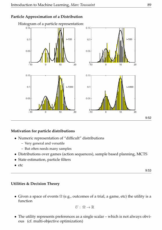
Introduction to Machine Learning, Marc Toussaint 89
Particle Approximation of a Distribution
Histogram of a particle representation:
9:52
Motivation for particle distributions
• Numeric representation of “difficult” distributions– Very general and versatile
– But often needs many samples
• Distributions over games (action sequences), sample based planning, MCTS• State estimation, particle filters• etc
9:53
Utilities & Decision Theory
• Given a space of events Ω (e.g., outcomes of a trial, a game, etc) the utility is afunction
U : Ω→ R
• The utility represents preferences as a single scalar – which is not always obvi-ous (cf. multi-objective optimization)

90 Introduction to Machine Learning, Marc Toussaint
• Decision Theory making decisions (that determine p(x)) that maximize expectedutility
EUp =
∫x
U(x) p(x)
• Concave utility functions imply risk aversion (and convex, risk-taking)9:54
Entropy
• The neg-log (− log p(x)) of a distribution reflects something like “error”:– neg-log of a Guassian↔ squared error
– neg-log likelihood↔ prediction error
• The (− log p(x)) is the “optimal” coding length you should assign to a symbolx. This will minimize the expected length of an encoding
H(p) =
∫x
p(x)[− log p(x)]
• The entropy H(p) = Ep(x)− log p(x) of a distribution p is a measure of uncer-tainty, or lack-of-information, we have about x
9:55
Kullback-Leibler divergence
• Assume you use a “wrong” distribution q(x) to decide on the coding length ofsymbols drawn from p(x). The expected length of a encoding is∫
x
p(x)[− log q(x)] ≥ H(p)
• The difference
D(p∣∣∣∣ q) =
∫x
p(x) logp(x)
q(x)≥ 0
is called Kullback-Leibler divergence
Proof of inequality, using the Jenson inequality:
−∫xp(x) log
q(x)
p(x)≥ − log
∫xp(x)
q(x)
p(x)= 0
9:56
Monte Carlo methods9:57
Introduction to Machine Learning, Marc Toussaint 91
Monte Carlo methods
• Generally, a Monte Carlo method is a method to generate a set of (potentiallyweighted) samples that approximate a distribution p(x).In the unweighted case, the samples should be i.i.d. xi ∼ p(x)
In the general (also weighted) case, we want particles that allow to estimateexpectations of anything that depends on x, e.g. f(x):
limN→∞
〈f(x)〉q = limN→∞
N∑i=1
wif(xi) =
∫x
f(x) p(x) dx = 〈f(x)〉p
In this view, Monte Carlo methods approximate an integral.• Motivation: p(x) itself is too complicated to express analytically or compute〈f(x)〉p directly
• Example: What is the probability that a solitair would come out successful? (Originalstory by Stan Ulam.) Instead of trying to analytically compute this, generate manyrandom solitairs and count.
• Naming: The method developed in the 40ies, where computers became faster. Fermi,Ulam and von Neumann initiated the idea. von Neumann called it “Monte Carlo” as acode name.
9:58
Rejection Sampling
• How can we generate i.i.d. samples xi ∼ p(x)?• Assumptions:
– We can sample x ∼ q(x) from a simpler distribution q(x) (e.g., uniform), calledproposal distribution
– We can numerically evaluate p(x) for a specific x (even if we don’t have an analyticexpression of p(x))
– There exists M such that ∀x : p(x) ≤ Mq(x) (which implies q has larger or equalsupport as p)
• Rejection Sampling:– Sample a candiate x ∼ q(x)
– With probability p(x)Mq(x)
accept x and add to S; otherwise reject
– Repeat until |S| = n
• This generates an unweighted sample set S to approximate p(x)9:59
Importance sampling
• Assumptions:
92 Introduction to Machine Learning, Marc Toussaint
– We can sample x ∼ q(x) from a simpler distribution q(x) (e.g., uniform)
– We can numerically evaluate p(x) for a specific x (even if we don’t have an analyticexpression of p(x))
• Importance Sampling:– Sample a candiate x ∼ q(x)
– Add the weighted sample (x, p(x)q(x)
) to S
– Repeat n times
• This generates an weighted sample set S to approximate p(x)
The weights wi = p(xi)q(xi)
are called importance weights
• Crucial for efficiency: a good choice of the proposal q(x)9:60
Applications
• MCTS estimates the Q-function at branchings in decision trees or games• Inference in graphical models (models involving many depending random vari-
ables)9:61
Some more continuous distributions
Gaussian N(x | a,A) = 1| 2πA | 1/2 e
− 12 (x−a)>A-1 (x−a)
Dirac or δ δ(x) = ∂∂xH(x)
Student’s t(=Gaussian for ν → ∞, otherwise heavytails)
p(x; ν) ∝ [1 + x2
ν ]−ν+1
2
Exponential(distribution over single event time)
p(x;λ) = [x ≥ 0] λe−λx
Laplace(“double exponential”)
p(x;µ, b) = 12be− | x−µ | /b
Chi-squared p(x; k) ∝ [x ≥ 0] xk/2−1e−x/2
Gamma p(x; k, θ) ∝ [x ≥ 0] xk−1e−x/θ
9:62
Introduction to Machine Learning, Marc Toussaint 93
10 Bayesian Regression & Classification
Learning as Inference
• The parameteric view
P (β|Data) =P (Data|β) P (β)
P (Data)=
Likelihood x PriorEvidence
• The function space view
P (f |Data) =P (Data|f) P (f)
P (Data)
• Today:– Bayesian (Kernel) Ridge Regression ↔ Gaussian Process (GP)– Bayesian (Kernel) Logistic Regression ↔ GP classification– Bayesian Neural Networks (briefly)
10:1
• Beyond learning about specific Bayesian learning methods:
Understand relations between
loss/error ↔ neg-log likelihood
regularization ↔ neg-log prior
cost (reg.+loss) ↔ neg-log posterior10:2
Gaussian Process = Bayesian (Kernel) Ridge Regression10:3
Ridge regression as Bayesian inference
• We have random variables X1:n, Y1:n, β
• We observe data D = (xi, yi)ni=1 and want to compute P (β |D)

94 Introduction to Machine Learning, Marc Toussaint
• Let’s assume:β
xi
yii = 1 : n
P (X) is arbitrary
P (β) is Gaussian: β ∼ N(0, σ2
λ ) ∝ e−λ
2σ2 ||β||2
P (Y |X,β) is Gaussian: y = x>β + ε , ε ∼ N(0, σ2)10:4
Ridge regression as Bayesian inference
• Bayes’ Theorem:
P (β |D) =P (D |β) P (β)
P (D)
P (β |x1:n, y1:n) =
∏ni=1 P (yi |β, xi) P (β)
Z
P (D |β) is a product of independent likelihoods for each observation (xi, yi)
Using the Gaussian expressions:
P (β |D) =1
Z ′
n∏i=1
e−1
2σ2 (yi−x>iβ)2
e−λ
2σ2 ||β||2
− logP (β |D) =1
2σ2
[ n∑i=1
(yi − x>iβ)2 + λ||β||2]
+ logZ ′
− logP (β |D) ∝ Lridge(β)
1st insight: The neg-log posterior P (β |D) is proportional to the cost functionLridge(β)!
10:5
Ridge regression as Bayesian inference
• Let us compute P (β |D) explicitly:
P (β |D) =1
Z′
n∏i=1
e− 1
2σ2 (yi−x>iβ)2
e− λ
2σ2 ||β||2
=1
Z′e− 1
2σ2
∑i(yi−x
>iβ)
2
e− λ
2σ2 ||β||2
=1
Z′e− 1
2σ2 [(y−Xβ)>(y−Xβ)+λβ>β]
=1
Z′e− 1
2[ 1σ2 y>y+ 1
σ2 β>(X>X+λI)β− 2
σ2 β>X>y]
= N(β | β,Σ)
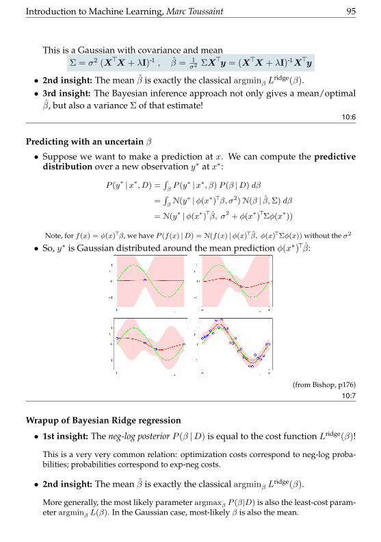
Introduction to Machine Learning, Marc Toussaint 95
This is a Gaussian with covariance and meanΣ = σ2 (X>X + λI)-1 , β = 1
σ2 ΣX>y = (X>X + λI)-1X>y
• 2nd insight: The mean β is exactly the classical argminβ Lridge(β).
• 3rd insight: The Bayesian inference approach not only gives a mean/optimalβ, but also a variance Σ of that estimate!
10:6
Predicting with an uncertain β
• Suppose we want to make a prediction at x. We can compute the predictivedistribution over a new observation y∗ at x∗:
P (y∗ |x∗, D) =∫βP (y∗ |x∗, β) P (β |D) dβ
=∫βN(y∗ |φ(x∗)>β, σ2) N(β | β,Σ) dβ
= N(y∗ |φ(x∗)>β, σ2 + φ(x∗)>Σφ(x∗))
Note, for f(x) = φ(x)>β, we have P (f(x) |D) = N(f(x) |φ(x)>β, φ(x)>Σφ(x)) without the σ2
• So, y∗ is Gaussian distributed around the mean prediction φ(x∗)>β:
(from Bishop, p176)10:7
Wrapup of Bayesian Ridge regression
• 1st insight: The neg-log posterior P (β |D) is equal to the cost function Lridge(β)!
This is a very very common relation: optimization costs correspond to neg-log proba-bilities; probabilities correspond to exp-neg costs.
• 2nd insight: The mean β is exactly the classical argminβ Lridge(β).
More generally, the most likely parameter argmaxβ P (β|D) is also the least-cost param-eter argminβ L(β). In the Gaussian case, most-likely β is also the mean.
96 Introduction to Machine Learning, Marc Toussaint
• 3rd insight: The Bayesian inference approach not only gives a mean/optimalβ, but also a variance Σ of that estimate!
This is a core benefit of the Bayesian view: It naturally provides a probability distribu-tion over predictions (“error bars”), not only a single prediction.
10:8
Kernel Bayesian Ridge Regression
• As in the classical case, we can consider arbitrary features φ(x)
• .. or directly use a kernel k(x, x′):
P (f(x) |D) = N(f(x) |φ(x)>β, φ(x)>Σφ(x))
φ(x)>β = φ(x)>X>(XX>+ λI)-1y
= κ(x)(K + λI)-1y
φ(x)>Σφ(x) = φ(x)>σ2 (X>X + λI)-1φ(x)
=σ2
λφ(x)>φ(x)− σ2
λφ(x)>X>(XX>+ λIk)-1Xφ(x)
=σ2
λk(x, x)− σ2
λκ(x)(K + λIn)-1κ(x)>
3rd line: As on slide 02:24last lines: Woodbury identity (A + UBV )-1 = A-1 − A-1U(B-1 + V A-1U)-1V A-1 withA = λI
• In standard conventions λ = σ2, i.e. P (β) = N(β|0, 1)
– Regularization: scale the covariance function (or features)10:9
Kernelized Bayesian Ridge Regression
is equivalent to Gaussian Processes(see also Welling: “Kernel Ridge Regression” Lecture Notes; Rasmussen & Williams sections 2.1 &6.2; Bishop sections 3.3.3 & 6)
• As we have the equations alreay, I skip further math details. (See Rasmussen& Williams)
10:10
Gaussian Processes
• The function space view
P (f |Data) =P (Data|f) P (f)
P (Data)
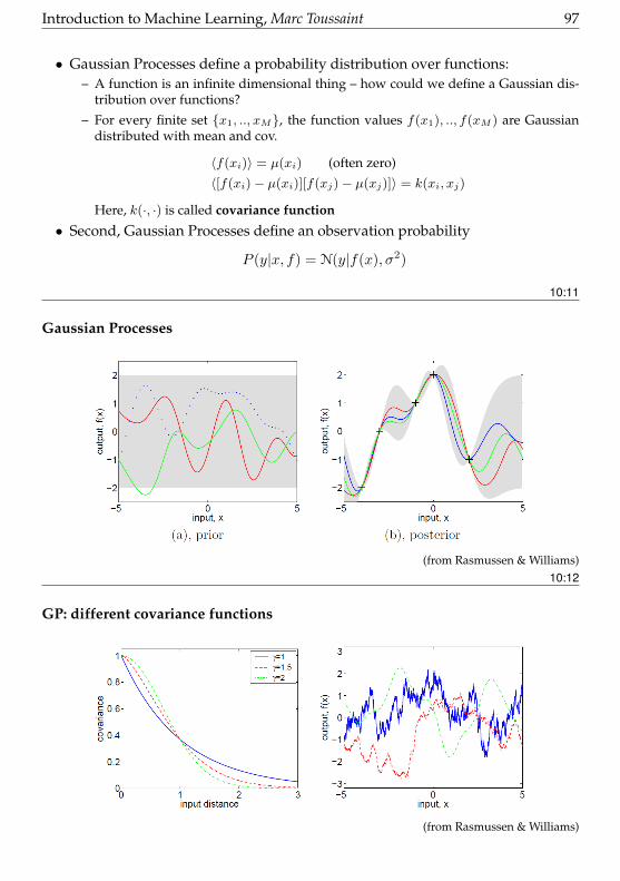
Introduction to Machine Learning, Marc Toussaint 97
• Gaussian Processes define a probability distribution over functions:– A function is an infinite dimensional thing – how could we define a Gaussian dis-
tribution over functions?
– For every finite set x1, .., xM, the function values f(x1), .., f(xM ) are Gaussiandistributed with mean and cov.
〈f(xi)〉 = µ(xi) (often zero)
〈[f(xi)− µ(xi)][f(xj)− µ(xj)]〉 = k(xi, xj)
Here, k(·, ·) is called covariance function
• Second, Gaussian Processes define an observation probability
P (y|x, f) = N(y|f(x), σ2)
10:11
Gaussian Processes
(from Rasmussen & Williams)10:12
GP: different covariance functions
(from Rasmussen & Williams)
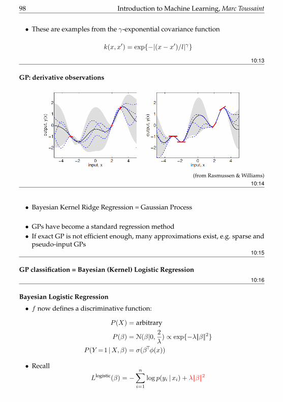
98 Introduction to Machine Learning, Marc Toussaint
• These are examples from the γ-exponential covariance function
k(x, x′) = exp−|(x− x′)/l|γ
10:13
GP: derivative observations
(from Rasmussen & Williams)10:14
• Bayesian Kernel Ridge Regression = Gaussian Process
• GPs have become a standard regression method• If exact GP is not efficient enough, many approximations exist, e.g. sparse and
pseudo-input GPs10:15
GP classification = Bayesian (Kernel) Logistic Regression10:16
Bayesian Logistic Regression
• f now defines a discriminative function:
P (X) = arbitrary
P (β) = N(β|0, 2
λ) ∝ exp−λ||β||2
P (Y =1 |X,β) = σ(β>φ(x))
• Recall
Llogistic(β) = −n∑i=1
log p(yi |xi) + λ||β||2
Introduction to Machine Learning, Marc Toussaint 99
• Again, the parameter posterior is
P (β|D) ∝ P (D |β) P (β) ∝ exp−Llogistic(β)
10:17
Bayesian Logistic Regression
• Use Laplace approximation (2nd order Taylor for L) at β∗ = argminβ L(β):
L(β) ≈ L(β∗) + β>∇+1
2β>Hβ , β = β − β∗
At β∗ the gradient∇ = 0 and L(β∗) = const. Therefore
P (β|D) ∝ exp−1
2β>Hβ
⇒ P (β|D) ≈ N(β|β∗, H -1)
• Then the predictive distribution of the discriminative function is also Gaussian!
P (f(x) |D) =∫βP (f(x) |β) P (β |D) dβ
≈∫βN(f(x) |φ(x)>β, 0) N(β |β∗, H -1) dβ
= N(f(x) |φ(x)>β∗, φ(x)>H -1φ(x)) =: N(f(x) | f∗, s2)
• The predictive distribution over the label y ∈ 0, 1:
P (y(x)=1 |D) =∫f(x)
σ(f(x)) P (f(x)|D) df
≈ σ((1 + s2π/8)-12 f∗)
which uses a probit approximation of the convolution.10:18
Kernelized Bayesian Logistic Regression
• As with Kernel Logistic Regression, the MAP discriminative function f∗ can befound iterating the Newton method↔ iterating GP estimation on a re-weighteddata set.• The rest is as above.
10:19
Kernel Bayesian Logistic Regression
is equivalent to Gaussian Process Classification
• GP classification became a standard classification method, if the predictionneeds to be a meaningful probability that takes the model uncertainty into ac-count.
10:20
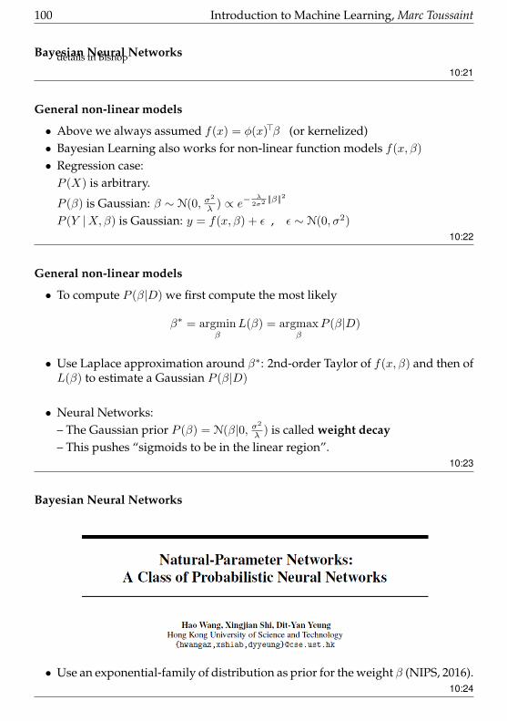
100 Introduction to Machine Learning, Marc Toussaint
Bayesian Neural Networksdetails in Bishop
10:21
General non-linear models
• Above we always assumed f(x) = φ(x)>β (or kernelized)• Bayesian Learning also works for non-linear function models f(x, β)
• Regression case:P (X) is arbitrary.
P (β) is Gaussian: β ∼ N(0, σ2
λ ) ∝ e−λ
2σ2 ||β||2
P (Y |X,β) is Gaussian: y = f(x, β) + ε , ε ∼ N(0, σ2)
10:22
General non-linear models
• To compute P (β|D) we first compute the most likely
β∗ = argminβ
L(β) = argmaxβ
P (β|D)
• Use Laplace approximation around β∗: 2nd-order Taylor of f(x, β) and then ofL(β) to estimate a Gaussian P (β|D)
• Neural Networks:– The Gaussian prior P (β) = N(β|0, σ
2
λ ) is called weight decay– This pushes “sigmoids to be in the linear region”.
10:23
Bayesian Neural Networks
• Use an exponential-family of distribution as prior for the weight β (NIPS, 2016).10:24
Introduction to Machine Learning, Marc Toussaint 101
Conclusions
• Probabilistic inference is a very powerful concept!– Inferring about the world given data– Learning, decision making, reasoning can view viewed as forms of (proba-bilistic) inference
• We introduced Bayes’ Theorem as the fundamental form of probabilistic infer-ence
• Marrying Bayes with (Kernel) Ridge (Logisic) regression yields– Gaussian Processes– Gaussian Process classification
10:25
102 Introduction to Machine Learning, Marc Toussaint
11 Graphical Models
Probabilistic Graphical Models
• The core difficulty in modelling is specifyingWhat are the relevant variables?
How do they depend on each other?
• Graphical Models are a simple, graphical notation for1) which random variables exist2) which random variables are “directly coupled”
Thereby they describe a joint probability distribution P (X1, .., Xn) over n randomvariables.
• 3 steps in Probabilistic Graphical Models– Representation, e.g. Bayesian Networks
– Inference, e.g. exact inference & approximate inference
– Learning, e.g. likelihood optimization11:1
Representation in Graphical Models
Here: Bayesian Networks (aka. directed model, belief network)11:2
Bayesian Networks
• A Bayesian Network is a– directed acyclic graph (DAG)
– where each node represents a random variable Xi– for each node we have a conditional probability distribution
P (Xi |Parents(Xi))
• In the simplest case (discrete RVs), the conditional distribution is representedas a conditional probability table (CPT)
11:3
Example
(Heckermann 1995)
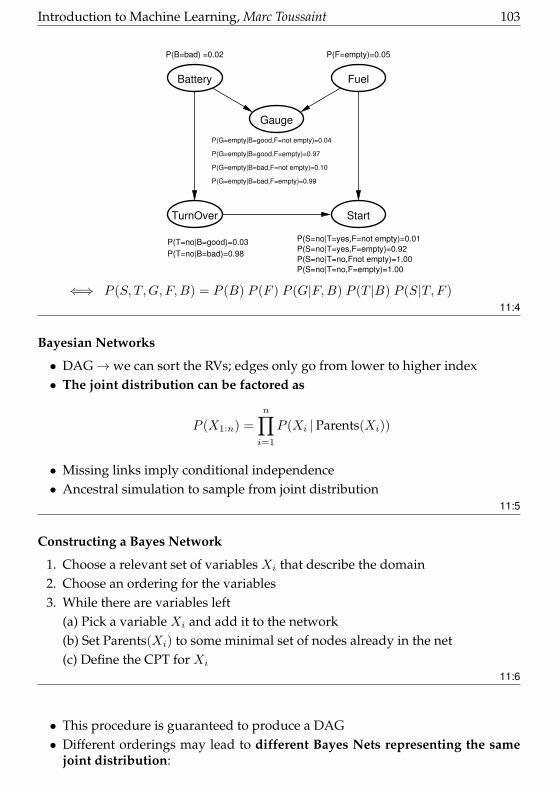
Introduction to Machine Learning, Marc Toussaint 103
P(G=empty|B=good,F=not empty)=0.04
P(G=empty|B=good,F=empty)=0.97
P(G=empty|B=bad,F=not empty)=0.10
P(G=empty|B=bad,F=empty)=0.99
P(T=no|B=good)=0.03
P(T=no|B=bad)=0.98
P(S=no|T=yes,F=not empty)=0.01
P(S=no|T=yes,F=empty)=0.92
P(S=no|T=no,Fnot empty)=1.00
P(S=no|T=no,F=empty)=1.00
Fuel
Gauge
Battery
TurnOver Start
P(B=bad) =0.02 P(F=empty)=0.05
⇐⇒ P (S, T,G, F,B) = P (B) P (F ) P (G|F,B) P (T |B) P (S|T, F )11:4
Bayesian Networks
• DAG→we can sort the RVs; edges only go from lower to higher index• The joint distribution can be factored as
P (X1:n) =
n∏i=1
P (Xi |Parents(Xi))
• Missing links imply conditional independence• Ancestral simulation to sample from joint distribution
11:5
Constructing a Bayes Network
1. Choose a relevant set of variables Xi that describe the domain2. Choose an ordering for the variables3. While there are variables left
(a) Pick a variable Xi and add it to the network(b) Set Parents(Xi) to some minimal set of nodes already in the net(c) Define the CPT for Xi
11:6
• This procedure is guaranteed to produce a DAG• Different orderings may lead to different Bayes Nets representing the same
joint distribution:

104 Introduction to Machine Learning, Marc Toussaint
• To ensure maximum sparsity choose a wise order (“root causes” first). Counterexample: construct DAG for the car example using the ordering S, T, G, F, B• “Wrong” ordering will give same joint distribution, but will require the speci-
fication of more numbers than otherwise necessary
11:7
Conditioning on Evidence
• Much of the point of Bayes Nets (and Graphical Models, more generally) is touse data or observed variables to infer the values of hidden (or latent) vari-ables.• We can condition on the observed variables and compute conditional distribu-
tions over the latent variables.
11:8
Bayes Nets & Conditional Independence
• Consider 3 simple independence structures that form the basic building blocksof all independence relationships representable by DAG
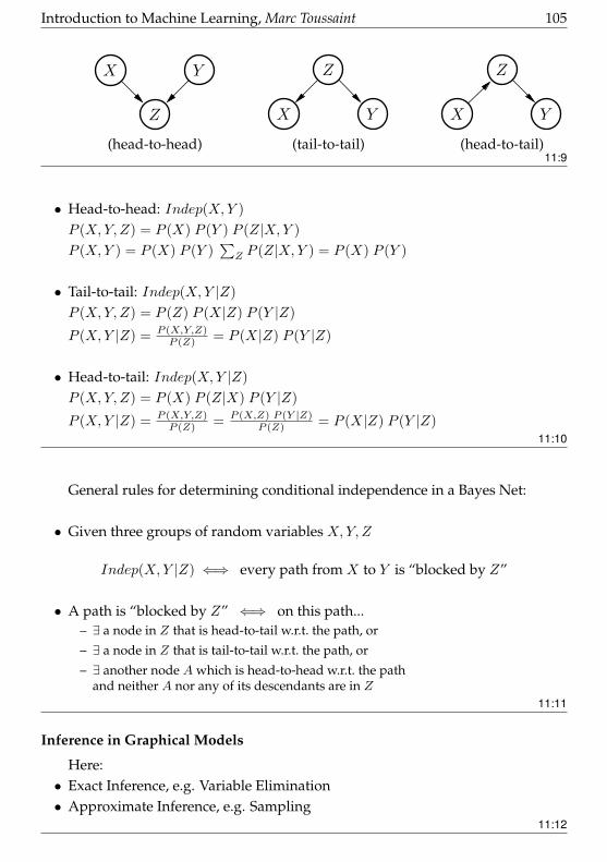
Introduction to Machine Learning, Marc Toussaint 105
Z
X Y
(head-to-head)
Z
X Y
(tail-to-tail)
Z
X Y
(head-to-tail)11:9
• Head-to-head: Indep(X,Y )
P (X,Y, Z) = P (X) P (Y ) P (Z|X,Y )
P (X,Y ) = P (X) P (Y )∑Z P (Z|X,Y ) = P (X) P (Y )
• Tail-to-tail: Indep(X,Y |Z)
P (X,Y, Z) = P (Z) P (X|Z) P (Y |Z)
P (X,Y |Z) = P (X,Y,Z)P (Z) = P (X|Z) P (Y |Z)
• Head-to-tail: Indep(X,Y |Z)
P (X,Y, Z) = P (X) P (Z|X) P (Y |Z)
P (X,Y |Z) = P (X,Y,Z)P (Z) = P (X,Z) P (Y |Z)
P (Z) = P (X|Z) P (Y |Z)11:10
General rules for determining conditional independence in a Bayes Net:
• Given three groups of random variables X,Y, Z
Indep(X,Y |Z) ⇐⇒ every path from X to Y is “blocked by Z”
• A path is “blocked by Z” ⇐⇒ on this path...– ∃ a node in Z that is head-to-tail w.r.t. the path, or
– ∃ a node in Z that is tail-to-tail w.r.t. the path, or
– ∃ another node A which is head-to-head w.r.t. the pathand neither A nor any of its descendants are in Z
11:11
Inference in Graphical Models
Here:• Exact Inference, e.g. Variable Elimination• Approximate Inference, e.g. Sampling
11:12
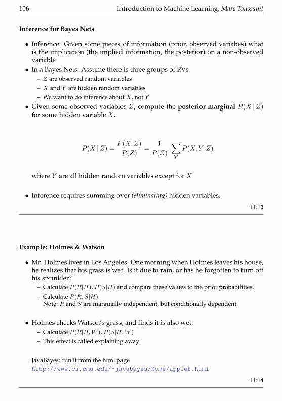
106 Introduction to Machine Learning, Marc Toussaint
Inference for Bayes Nets
• Inference: Given some pieces of information (prior, observed variabes) whatis the implication (the implied information, the posterior) on a non-observedvariable• In a Bayes Nets: Assume there is three groups of RVs
– Z are observed random variables
– X and Y are hidden random variables
– We want to do inference about X , not Y
• Given some observed variables Z, compute the posterior marginal P (X |Z)for some hidden variable X .
P (X |Z) =P (X,Z)
P (Z)=
1
P (Z)
∑Y
P (X,Y, Z)
where Y are all hidden random variables except for X
• Inference requires summing over (eliminating) hidden variables.
11:13
Example: Holmes & Watson
• Mr. Holmes lives in Los Angeles. One morning when Holmes leaves his house,he realizes that his grass is wet. Is it due to rain, or has he forgotten to turn offhis sprinkler?
– Calculate P (R|H), P (S|H) and compare these values to the prior probabilities.
– Calculate P (R,S|H).Note: R and S are marginally independent, but conditionally dependent
• Holmes checks Watson’s grass, and finds it is also wet.– Calculate P (R|H,W ), P (S|H,W )
– This effect is called explaining away
JavaBayes: run it from the html pagehttp://www.cs.cmu.edu/˜javabayes/Home/applet.html
11:14
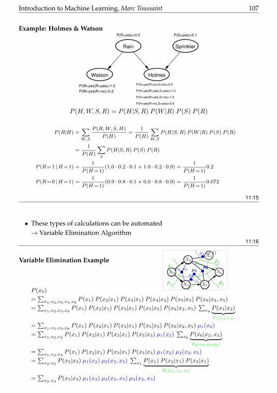
Introduction to Machine Learning, Marc Toussaint 107
Example: Holmes & Watson
Watson Holmes
P(W=yes|R=yes)=1.0
P(W=yes|R=no)=0.2 P(H=yes|R=yes,S=yes)=1.0
P(H=yes|R=yes,S=no)=1.0
P(H=yes|R=no,S=yes)=0.9
P(H=yes|R=no,S=no)=0.0
Rain
P(R=yes)=0.2
Sprinkler
P(S=yes)=0.1
P (H,W,S,R) = P (H|S,R) P (W |R) P (S) P (R)
P (R|H) =∑W,S
P (R,W,S,H)
P (H)=
1
P (H)
∑W,S
P (H|S,R) P (W |R) P (S) P (R)
=1
P (H)
∑S
P (H|S,R) P (S) P (R)
P (R=1 |H=1) =1
P (H=1)(1.0 · 0.2 · 0.1 + 1.0 · 0.2 · 0.9) =
1
P (H=1)0.2
P (R=0 |H=1) =1
P (H=1)(0.9 · 0.8 · 0.1 + 0.0 · 0.8 · 0.9) =
1
P (H=1)0.072
11:15
• These types of calculations can be automated→ Variable Elimination Algorithm
11:16
Variable Elimination Example
X6
X3 X5
X4X2
X1 X6
X3 X5
X4X2
X1
F1
µ1 (≡ 1)
X6
X3 X5
X2
X1 X6
X3 X5
X2
X1
F2
µ2
X3 X5
X2
X1
µ2
X3 X5
X2
X1
F3
µ2µ3
X3 X5
X2
µ2µ3
X3 X5
X2
F4µ4
X3 X5
µ4
X3 X5
F5
µ5
X5
P (x5)
=∑x1,x2,x3,x4,x6
P (x1) P (x2|x1) P (x3|x1) P (x4|x2) P (x5|x3) P (x6|x2, x5)
=∑x1,x2,x3,x6
P (x1) P (x2|x1) P (x3|x1) P (x5|x3) P (x6|x2, x5)∑x4P (x4|x2)︸ ︷︷ ︸F1(x2,x4)
=∑x1,x2,x3,x6
P (x1) P (x2|x1) P (x3|x1) P (x5|x3) P (x6|x2, x5) µ1(x2)
=∑x1,x2,x3
P (x1) P (x2|x1) P (x3|x1) P (x5|x3) µ1(x2)∑x6P (x6|x2, x5)︸ ︷︷ ︸F2(x2,x5,x6)
=∑x1,x2,x3
P (x1) P (x2|x1) P (x3|x1) P (x5|x3) µ1(x2) µ2(x2, x5)
=∑x2,x3
P (x5|x3) µ1(x2) µ2(x2, x5)∑x1P (x1) P (x2|x1) P (x3|x1)︸ ︷︷ ︸
F3(x1,x2,x3)
=∑x2,x3
P (x5|x3) µ1(x2) µ2(x2, x5) µ3(x2, x3)

108 Introduction to Machine Learning, Marc Toussaint
=∑x3P (x5|x3)
∑x2µ1(x2) µ2(x2, x5) µ3(x2, x3)︸ ︷︷ ︸
F4(x3,x5)
=∑x3P (x5|x3) µ4(x3, x5)
=∑x3P (x5|x3) µ4(x3, x5)︸ ︷︷ ︸
F5(x3,x5)
= µ5(x5)
11:17
Variable Elimination Example – lessons learnt
• There is a dynamic programming principle behind Variable Elimination:– For eliminating X5,4,6 we use the solution of eliminating X4,6
– The “sub-problems” are represented by the F terms, their solutions by the remainingµ terms
• The factorization of the joint– determines in which order Variable Elimination is efficient
– determines what the terms F (...) and µ(...) depend on
• We can automate Variable Elimination. For the automation, all that matters isthe factorization of the joint• For densely connected graphs, exact inference may be intractable.• There are 2 widely used approximation schemes
– Markov chain Monte Carlo (MCMC): simulate lots of values of the variables anduse the sample frequencies to approximate probabilities
– Variational inference: Approximate the graph with a simplified the graph (with nocycles) and fit a set of “variational” parameters such that the probabilities computedwith the simple structure are “close” to those in the original graph
11:18
Sampling
• Read Andrieu et al: An Introduction to MCMC for Machine Learning (MachineLearning, 2003)
• Here I’ll discuss only 2 basic methods:– Rejection sampling
– Importance sampling11:19
Rejection Sampling
• We have a Bayesian Network with RVs X1:n, some of which are observed:Xobs = yobs, obs ⊂ 1 : n
Introduction to Machine Learning, Marc Toussaint 109
• The goal is to compute marginal posteriors P (Xi |Xobs = yobs) conditioned onthe observations.
• Our strategy is to generate a set of K (joint) samples of all variables
S = (xk1 , xk2 , .., xkn)Kk=1
Note: Each sample xk1:n is a list of instantiation of all RVs.11:20
Rejection Sampling
• To generate a single sample xk1:n:
1. Sort all RVs in topological order; start with i = 1
2. a) Sample a value xki ∼ P (Xi |xkParents(i)) for the ith RV conditional to theprevious samples xk1:i-1
b) If i ∈ obs compare the sampled value xki with the observation yi. Rejectand repeat from a) if the sample is not equal to the observation.
3. Repeat with i← i+ 1 from 2.
11:21
Rejection Sampling
• Since computers are fast, we can sample for large K• The sample set
S = (xk1 , xk2 , .., xkn)Kk=1
implies the necessary information:• We can compute the marginal probabilities from these statistics:
P (Xi=x |Xobs = yobs) ≈countS(xki = x)
K
or pair-wise marginals:
P (Xi=x,Xj=x′ |Xobs = yobs) ≈countS(xki = x ∧ xkj = x′)
K
11:22
Importance sampling (with likelihood weighting)
• Rejecting whole samples may become very inefficient in large Bayes Nets!
110 Introduction to Machine Learning, Marc Toussaint
• New strategy: We generate a weighted sample set
S = (wk, xk1 , xk2 , .., xkn)Kk=1
where each samples xk1:n is associated with a weight wk
• In our case, we will choose the weights proportional to the likelihood P (Xobs =yobs |X1:n=xk1:n) of the observations conditional to the sample xk1:n
11:23
Importance sampling
• To generate a single sample (wk, xk1:n):
1. Sort all RVs in topological order; start with i = 1 and wk = 1
2. a) If i 6∈ obs, sample a value xki ∼ P (Xi |xkParents(i)) for the ith RV condi-tional to the previous samples xk1:i-1
b) If i ∈ obs, set the value xki = yi and update the weight according tolikelihood
wk ← wk P (Xi=yi |xk1:i-1)
3. Repeat with i← i+ 1 from 2.
11:24
Importance Sampling (with likelihood weighting)
• From the weighted sample set
S = (wk, xk1 , xk2 , .., xkn)Kk=1
• We can compute the marginal probabilities:
P (Xi=x |Xobs = yobs) ≈∑Kk=1 w
k[xki = x]∑Kk=1 w
k
and likewise pair-wise marginals, etc
Notation: [expr] = 1 if expr is true and zero otherwise11:25
Sampling – conclusions
• Sampling algorithms are very simple, very general and very popular– they equally work for continuous & discrete RVs
– one only needs to ensure/implement the ability to sample from conditional distri-butions, no further algebraic manipulations
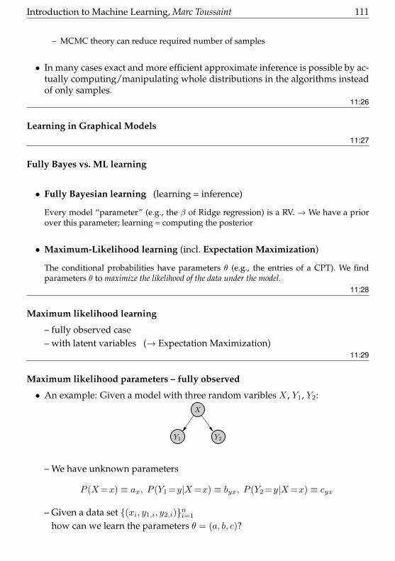
Introduction to Machine Learning, Marc Toussaint 111
– MCMC theory can reduce required number of samples
• In many cases exact and more efficient approximate inference is possible by ac-tually computing/manipulating whole distributions in the algorithms insteadof only samples.
11:26
Learning in Graphical Models11:27
Fully Bayes vs. ML learning
• Fully Bayesian learning (learning = inference)
Every model “parameter” (e.g., the β of Ridge regression) is a RV.→ We have a priorover this parameter; learning = computing the posterior
• Maximum-Likelihood learning (incl. Expectation Maximization)
The conditional probabilities have parameters θ (e.g., the entries of a CPT). We findparameters θ to maximize the likelihood of the data under the model.
11:28
Maximum likelihood learning
– fully observed case– with latent variables (→ Expectation Maximization)
11:29
Maximum likelihood parameters – fully observed
• An example: Given a model with three random varibles X , Y1, Y2:X
Y1 Y2
– We have unknown parameters
P (X=x) ≡ ax, P (Y1 =y|X=x) ≡ byx, P (Y2 =y|X=x) ≡ cyx
– Given a data set (xi, y1,i, y2,i)ni=1
how can we learn the parameters θ = (a, b, c)?
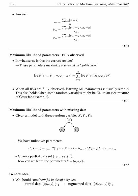
112 Introduction to Machine Learning, Marc Toussaint
• Answer:
ax =
∑ni=1[xi=x]
n
byx =
∑ni=1[y1,i=y ∧ xi=x]
nax
cyx =
∑ni=1[y2,i=y ∧ xi=x]
nax
11:30
Maximum likelihood parameters – fully observed
• In what sense is this the correct answer?→ These parameters maximize observed data log-likelihood
logP (x1:n, y1,1:N , y2,1:n; θ) =
n∑i=1
logP (xi, y1,i, y2,i ; θ)
• When all RVs are fully observed, learning ML parameters is usually simple.This also holds when some random variables might be Gaussian (see mixtureof Gaussians example).
11:31
Maximum likelihood parameters with missing data
• Given a model with three random varibles X , Y1, Y2:X
Y2Y1
– We have unknown parameters
P (X=x) ≡ ax, P (Y1 =y|X=x) ≡ byx, P (Y2 =y|X=x) ≡ cyx
– Given a partial data set (y1,i, y2,i)Ni=1
how can we learn the parameters θ = (a, b, c)?11:32
General idea
• We should somehow fill in the missing datapartial data (y1:2,i)ni=1 → augmented data (xi, y1:2,i)ni=1
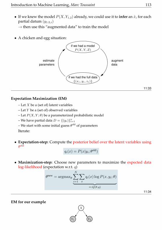
Introduction to Machine Learning, Marc Toussaint 113
• If we knew the model P (X,Y1,2) already, we could use it to infer an xi for eachpartial datum (y1:2,i)
→ then use this “augmented data” to train the model
• A chicken and egg situation:
(xi, yi, zi)if we had the full data
dataaugment
P (X,Y, Z)
if we had a model
estimateparameters
11:33
Expectation Maximization (EM)
– Let X be a (set of) latent variables– Let Y be a (set of) observed variables– Let P (X,Y ; θ) be a parameterized probabilistic model– We have partial data D = (yi)ni=1
– We start with some initial guess θold of parameters
Iterate:
• Expectation-step: Compute the posterior belief over the latent variables usingθold
qi(x) = P (x|yi; θold)
• Maximization-step: Choose new parameters to maximize the expected datalog-likelihood (expectation w.r.t. q)
θnew = argmaxθ
N∑i=1
∑x
qi(x) logP (x, yi; θ)︸ ︷︷ ︸=:Q(θ,q)
11:34
EM for our exampleX
Y2Y1
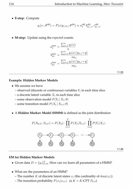
114 Introduction to Machine Learning, Marc Toussaint
• E-step: Compute
qi(x ; θold) = P (x|y1:2,i; θold) ∝ aold
x boldy1,ix c
oldy1,ix
• M-step: Update using the expected counts:
anewx =
∑ni=1 qi(x)
n
bnewyx =
∑ni=1 qi(x) [y1,i=y]
nax
cnewyx =
∑ni=1 qi(x) [y2,i=y]
nax
11:35
Example: Hidden Markov Models
• We assume we have– observed (discrete or continuous) variables Yt in each time slice– a discrete latent variable Xt in each time slice– some observation model P (Yt |Xt; θ)
– some transition model P (Xt |Xt-1; θ)
• A Hidden Markov Model (HMM) is defined as the joint distribution
P (X0:T , Y0:T ) = P (X0) ·T∏t=1
P (Xt|Xt-1) ·T∏t=0
P (Yt|Xt) .
X0 X1 X2 X3
Y0 Y1 Y2 Y3 YT
XT
11:36
EM for Hidden Markov Models
• Given data D = ytTt=0. How can we learn all parameters of a HMM?
• What are the parameters of an HMM?– The number K of discrete latent states xt (the cardinality of dom(xt))– The transition probability P (xt|xt-1) (a K ×K-CPT Pk′k)
Introduction to Machine Learning, Marc Toussaint 115
– The initial state distribution P (x0) (a K-table πk)– Parameters of the output distribution P (yt |xt=k)
e.g., the mean µk and covariance matrix Σk for each latent state k
• Learning K is very hard!– Try and evaluate many K– Have a distribution over K (→ infinite HMMs)– We assume K fixed in the following
• Learning the other parameters is easier: Expectation Maximization11:37
EM for Hidden Markov Models
The paramers of an HMM are θ = (Pk′k, πk, µk,Σk)
• E-step: Compute the marginal posteriors (also pair-wise)q(xt) = P (xt | y1:T ; θold)
q(xt, xt+1) = P (xt, xt+1 | y1:T ; θold)
• M-step: Update the parameters
Pk′k ←∑T -1t=0 q(xt=k, xt+1 =k′)∑T -1
t=0 q(xt=k), πk ← q(x0 =k)
µk ←T∑t=0
wktyt , Σk ←T∑t=0
wkt yty>t − µkµ>k
with wkt = q(xt=k)/(∑Tt=0 q(xt=k)) (each row of wkt is normalized)
compare with EM for Gaussian Mixtures!11:38
Summary
• Probabilistic Graphical Model is a powerful tool to model complex dependen-cies between variables• Inference and learning are often very computational intensiv. Approximation
is neccessary• Not discussed: Causal inference
11:39