introduction to learning lecture 2people.csail.mit.edu/dsontag/courses/ml13/slides/lecture... ·...
TRANSCRIPT
Introduction to Learning Lecture 2
David Sontag
New York University
Slides adapted from Luke Zettlemoyer, Vibhav Gogate, Pedro Domingos, and Carlos Guestrin

Hypo. Space: Degree-N Polynomials
x
t
M = 0
0 1
−1
0
1
x
t
M = 1
0 1
−1
0
1
x
t
M = 3
0 1
−1
0
1
x
t
M = 9
0 1
−1
0
1
M
ER
MS
0 3 6 90
0.5
1TrainingTest
Learning curve
Measure of model complexity
For regression, a common choice is squared loss:
The empirical loss of the function f applied to the training data is then:
Example of overfitting
We measure error using a loss function
Squared error

Occam’s Razor Principle
• William of Occam: Monk living in the 14th century
• Principle of parsimony:
“One should not increase, beyond what is necessary, the number of entities required to explain anything”
• When many solutions are available for a given problem, we should select the simplest one
• But what do we mean by simple?
• We will use prior knowledge of the problem to solve to define what is a simple solution
[Samy Bengio]
Example of a prior: smoothness
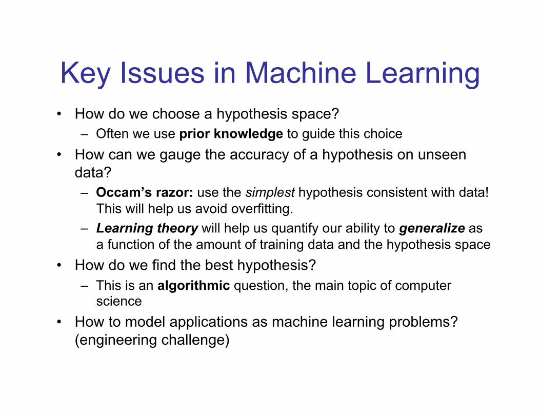
Key Issues in Machine Learning • How do we choose a hypothesis space?
– Often we use prior knowledge to guide this choice
• How can we gauge the accuracy of a hypothesis on unseen data? – Occam’s razor: use the simplest hypothesis consistent with data!
This will help us avoid overfitting.
– Learning theory will help us quantify our ability to generalize as a function of the amount of training data and the hypothesis space
• How do we find the best hypothesis? – This is an algorithmic question, the main topic of computer
science
• How to model applications as machine learning problems? (engineering challenge)

Binary classification
• Input: email • Output: spam/ham • Setup:
– Get a large collection of example emails, each labeled “spam” or “ham”
– Note: someone has to hand label all this data!
– Want to learn to predict labels of new, future emails
• Features: The attributes used to make the ham / spam decision – Words: FREE! – Text Patterns: $dd, CAPS – Non-text: SenderInContacts – …
Dear Sir.
First, I must solicit your confidence in this transaction, this is by virture of its nature as being utterly confidencial and top secret. …
TO BE REMOVED FROM FUTURE MAILINGS, SIMPLY REPLY TO THIS MESSAGE AND PUT "REMOVE" IN THE SUBJECT.
99 MILLION EMAIL ADDRESSES FOR ONLY $99
Ok, Iknow this is blatantly OT but I'm beginning to go insane. Had an old Dell Dimension XPS sitting in the corner and decided to put it to use, I know it was working pre being stuck in the corner, but when I plugged it in, hit the power nothing happened.
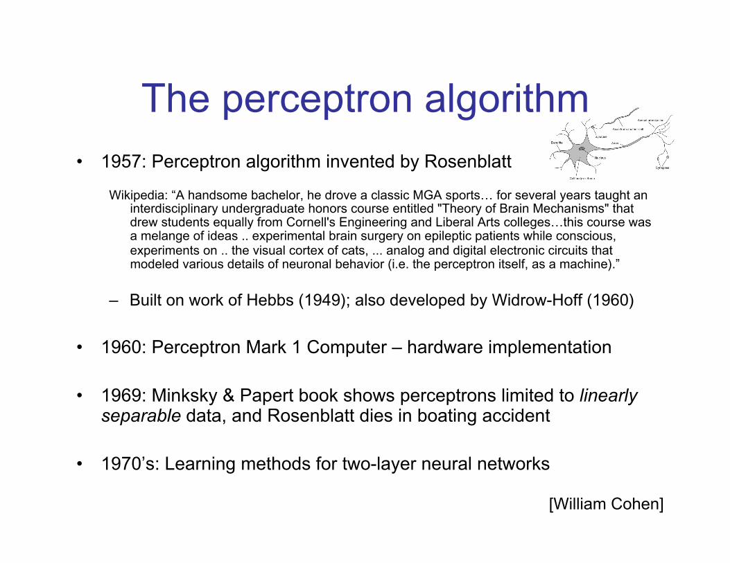
The perceptron algorithm • 1957: Perceptron algorithm invented by Rosenblatt
Wikipedia: “A handsome bachelor, he drove a classic MGA sports… for several years taught an interdisciplinary undergraduate honors course entitled "Theory of Brain Mechanisms" that drew students equally from Cornell's Engineering and Liberal Arts colleges…this course was a melange of ideas .. experimental brain surgery on epileptic patients while conscious, experiments on .. the visual cortex of cats, ... analog and digital electronic circuits that modeled various details of neuronal behavior (i.e. the perceptron itself, as a machine).”
– Built on work of Hebbs (1949); also developed by Widrow-Hoff (1960)
• 1960: Perceptron Mark 1 Computer – hardware implementation
• 1969: Minksky & Papert book shows perceptrons limited to linearly separable data, and Rosenblatt dies in boating accident
• 1970’s: Learning methods for two-layer neural networks
[William Cohen]

Linear Classifiers
• Inputs are feature values • Each feature has a weight • Sum is the activation
• If the activation is: – Positive, output class 1 – Negative, output class 2 Σ
f1
f2
f3
w1
w2
w3 >0?
Important note: changing notation!
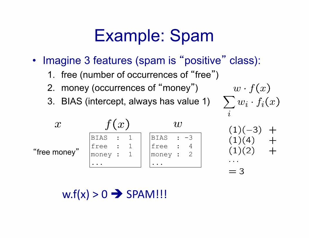
Example: Spam • Imagine 3 features (spam is “positive” class):
1. free (number of occurrences of “free”)
2. money (occurrences of “money”)
3. BIAS (intercept, always has value 1)
BIAS : -3 free : 4 money : 2 ...
BIAS : 1 free : 1 money : 1 ...
“free money”
w.f(x) > 0 SPAM!!!

Binary Decision Rule • In the space of feature vectors
– Examples are points
– Any weight vector is a hyperplane
– One side corresponds to Y=+1
– Other corresponds to Y=-1
BIAS : -3 free : 4 money : 2 ... 0 1
0
1
2
free m
oney
+1 = SPAM
-1 = HAM
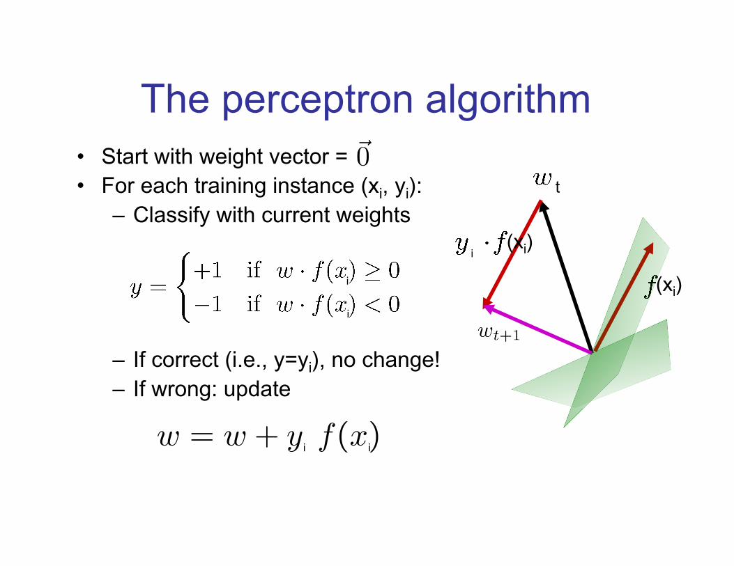
The perceptron algorithm • Start with weight vector = • For each training instance (xi, yi):
– Classify with current weights
– If correct (i.e., y=yi), no change! – If wrong: update
= ln
�
⇧⇧⇤
1⇥i⇤2�
e� (xi�µi0)
2
2�2i
1⇥i⇤2�
e� (xi�µi1)
2
2�2i
⇥
⌃⌃⌅
= �(xi � µi0)2
2⇤2i+(xi � µi1)2
2⇤2i
=µi0 + µi1
⇤2ixi +
µ2i0 + µ2i12⇤2i
w0 = ln1� ⇥
⇥+
µ2i0 + µ2i12⇤2i
wi =µi0 + µi1
⇤2i
w = w + �⌥
j
[y⇥j � p(y⇥j |xj , w)]f(xj)
w = w + [y⇥ � y(x;w)]f(x)
w = w + y⇥f(x)
4
i
i
i i
(xi)
(xi) i
t
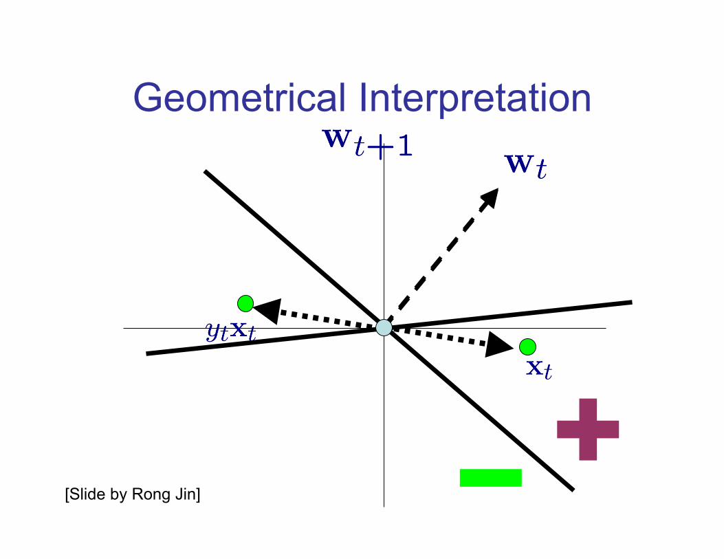
Geometrical Interpretation
[Slide by Rong Jin]

What questions should we ask about a learning algorithm?
• What is the perceptron algorithm’s running time?
• If a weight vector with small training error exists, will perceptron find it?
• How well does the resulting classifier generalize to unseen data?

Linearly Separable
Called the functional margin with respect to the training set
Equivalently, for yt = +1,
and for yt = -1,
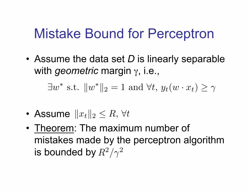
Mistake Bound for Perceptron
• Assume the data set D is linearly separable with geometric margin γ, i.e.,
• Assume
• Theorem: The maximum number of mistakes made by the perceptron algorithm is bounded by
kxtk2 R, 8t
9w⇤ s.t. kw⇤k2 = 1 and 8t, yt(w · xt) � �

Proof by induction
[Slide by Rong Jin]
. .
(full proof given on board)
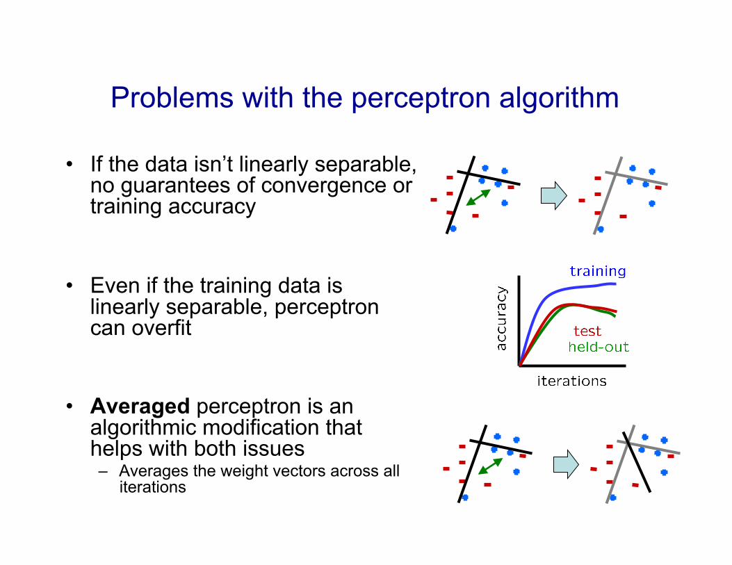
Problems with the perceptron algorithm
• If the data isn’t linearly separable, no guarantees of convergence or training accuracy
• Even if the training data is linearly separable, perceptron can overfit
• Averaged perceptron is an algorithmic modification that helps with both issues – Averages the weight vectors across all
iterations
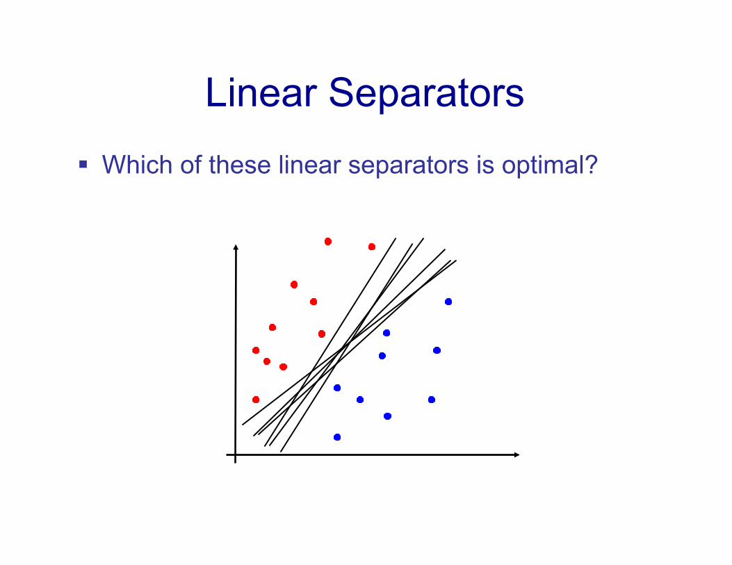
Linear Separators
Which of these linear separators is optimal?
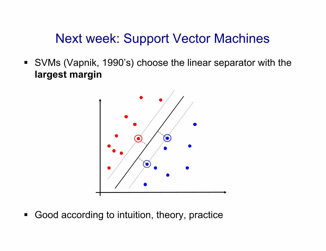
Next week: Support Vector Machines
SVMs (Vapnik, 1990’s) choose the linear separator with the largest margin
Good according to intuition, theory, practice

ML Methodology • Data: labeled instances, e.g. emails marked spam/ham
– Training set – Held out set (sometimes call Validation set) – Test set
Randomly allocate to these three, e.g. 60/20/20
• Features: attribute-value pairs which characterize each x
• Experimentation cycle – Select a hypothesis f (Tune hyperparameters on held-out or validation set)
– Compute accuracy of test set
– Very important: never “peek” at the test set!
• Evaluation – Accuracy: fraction of instances predicted correctly
Training Data
Held-Out Data
Test Data