AC 2011-2237: INTRODUCTION TO INSTRUMENTATION AND CON-TROL SYSTEMS USING A PENDULUM MOUNTED AIR ROCKET

Michael Keller, University of Tulsa

Michael Keller is an assistant professor of mechanical engineering at the university of tulsa. His researchand teaching interests are in solid mechanics, both experimental and theoretical, and materials science.

Jeremy S. Daily, University of Tulsa

c©American Society for Engineering Education, 2011

Introduction to Instrumentation and ControlSystems Using a Pendulum Mounted Air Rocket

AbstractCourses on engineering instrumentation and measurement typically have two objectives: 1)introducing the students to essential and modern engineering instrumentation and 2) developingthe ability of students to plan, execute, and analyze engineering experiments. The projectdescribed in this paper encompasses all of these objectives and introduces students to practicalaspects of control systems. The multi-week laboratory exercise requires the students to interfacewith laboratory hardware and modern instrumentation with only limited guidance from theinstructor. The self-guided problem solving approach to instrumentation gives students a deeperunderstanding of the nuances and complexity of developing and implementing multi-componentinstrumentation systems. Additionally, the students are required to develop a limited controlsystem that fires an air rocket in response to position or acceleration feedback in order to achievethe highest swing height. Since this class precedes the formal controls systems course in ourcurriculum, conceptual control system theory is provided in a one-on-one basis in the lab. Inessence the laboratory serves as a ‘just-in-time’ controls course and sets up the formalmathematical controls course that follows. This paper includes the detailed design of the airrocket thrust laboratory apparatus and computerized data acquisition setup. Schematics andspecifications of the instruments are included along with a typical student data and analysis.Finally, student surveys were conducted and analyzed to assess the both general and specificoutcomes of the laboratory experience.IntroductionMeasurement and instrumentation courses are typically the ‘catch-all’ course for topics inexperimental design and execution in mechanical engineering curriculum. Course objectivesinclude the introduction of modern data acquisition systems and techniques, the development andpresentation of statistical techniques for data analysis, and the introduction of formal uncertaintyanalysis. These three course topics are employed in nearly every rigorous engineering experimentthat a student would perform in either an industrial setting or during advanced graduate research.However, most laboratory experiments are ‘canned’ and handed to the student with a detailedprocedure that can be easily followed. The emphasis on these experiments is not the experiment,but the analysis of the data generated from a particular experiment. Essentially, these laboratoriescan quickly degenerate into a show-and-tell theater portion followed by individual student workduring the data analysis and report writing phases.1

Recently, self-directed and autonomous learning experiences have been realized to be integral tothe learning process. In order to introduce these aspects into an instrument and measurementcourse setting, a defined, but undirected instrumentation lab was recently designed andimplemented in the Department of Mechanical Engineering at The University of Tulsa. This labwas based on an existing air-rocket lab that had been almost entirely demonstrative in previousiterations.3,2 In this lab, a fire-extinguisher air rocket is attached to a bearing-suspendedpendulum, instrumented and mounted to a frame. Students are directed to connect, calibrate, andwrite a data acquisition program in LabVIEW in order to collect data during a short duration fire

of the rocket, typically lasting 1 to 3 seconds. The data gathered during this lab is used to generatean impulse vs. initial pressure curve to determine the potential for using an air rocket to powercomical human flight. After the data acquisition program is completed, a follow-on lab period isdevoted to the programming of a simple control system in LabVIEW with the goal of achievingthe highest swing height for a given initial pressure. This is the capstone lab of the course andcomes after 4 dedicated LabVIEW programing labs and two previous, directed labs usingLabVIEW to interface with data acquisition (DAQ) hardware. Some previous familiarity with thepractical aspects of DAQ implementation is critical to the success of this experiment.Description of the Lab Exercise

Figure 1: Physical arrangement of the rocket teststand, with the transducer locations indicated.

The goal of this is lab is two-fold.1) Determine the thrust characteristicsof a simple, pendulum attached,pressurized air rocket and 2) constructa simple control system that attains thehighest possible swing height for a giveninitial rocket pressure. This experimentintroduces the students to data acquisitionand signal output for both analogand digital sensors. The controls aspect,while technically simple, introducesstudents to the concept of feedback andboolean logic. The physical experimentalapparatus is shown in Fig. 1.Students are given only basic informationabout the sensors that might be gatheredfrom a data sheet. Table 1 lists theinformation that the students are given foreach sensor. All sensors are terminated at aterminal strip at the top of the rocket frame.An example pinout is listed in Table 2and is provided to the students.After a brief introduction to the laband a description of each of the sensors,the students are given three LabVIEWcompact DAQ modules, a bridge sensormodule (NI 9237), a digital input/outputmodule (NI 9401), and a differentialdigital input module (NI 9411). Hook upwire is available for the students as well as all the required break-out boards and basic equipment.The students are verbally directed to spend the first lab period physically connecting the sensorsto the DAQ hardware and writing LabVIEW programs to take data from the sensors and generatea digital signal to operate the solenoid valve. The second lab period is spent calibrating thepressure transducer and accelerometer and taking the data required for the analysis of the rocket

impulse. The third lab period is spent designing and implementing the control system. Details ofthe data analysis are provided below. After the data analysis is performed, the students are alsorequired to complete a detailed uncertainty analysis of the experiment based on given uncertaintyvalues. The details of the uncertainty analysis are also given in a section below.

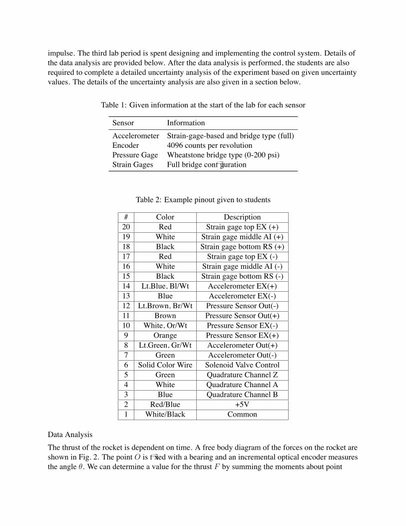
Table 1: Given information at the start of the lab for each sensor

Sensor InformationAccelerometer Strain-gage-based and bridge type (full)Encoder 4096 counts per revolutionPressure Gage Wheatstone bridge type (0-200 psi)Strain Gages Full bridge configuration

Table 2: Example pinout given to students

# Color Description20 Red Strain gage top EX (+)19 White Strain gage middle AI (+)18 Black Strain gage bottom RS (+)17 Red Strain gage top EX (-)16 White Strain gage middle AI (-)15 Black Strain gage bottom RS (-)14 Lt.Blue, Bl/Wt Accelerometer EX(+)13 Blue Accelerometer EX(-)12 Lt.Brown, Br/Wt Pressure Sensor Out(-)11 Brown Pressure Sensor Out(+)10 White, Or/Wt Pressure Sensor EX(-)9 Orange Pressure Sensor EX(+)8 Lt.Green, Gr/Wt Accelerometer Out(+)7 Green Accelerometer Out(-)6 Solid Color Wire Solenoid Valve Control5 Green Quadrature Channel Z4 White Quadrature Channel A3 Blue Quadrature Channel B2 Red/Blue +5V1 White/Black Common

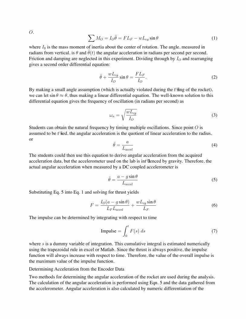
Data AnalysisThe thrust of the rocket is dependent on time. A free body diagram of the forces on the rocket areshown in Fig. 2. The point O is fixed with a bearing and an incremental optical encoder measuresthe angle θ. We can determine a value for the thrust F by summing the moments about point

O. ∑MO = IOθ̈ = FLF − wLcg sin θ (1)

where I0 is the mass moment of inertia about the center of rotation. The angle, measured inradians from vertical, is θ and θ̈(t) the angular acceleration in radians per second per second.Friction and damping are neglected in this experiment. Dividing through by IO and rearranginggives a second order differential equation:

θ̈ +wLcg

IOsin θ =

FLF

IO. (2)

By making a small angle assumption (which is actually violated during the firing of the rocket),we can let sin θ ≈ θ, thus making a linear differential equation. The well-known solution to thisdifferential equation gives the frequency of oscillation (in radians per second) as

ωn =

√wLcg

IO(3)

Students can obtain the natural frequency by timing multiple oscillations. Since point O isassumed to be fixed, the angular acceleration is the quotient of linear acceleration to the radius,or

θ̈ =a

Laccel

(4)

The students could then use this equation to derive angular acceleration from the acquiredacceleration data, but the accelerometer used on the lab is influenced by gravity. Therefore, theactual angular acceleration when measured by a DC coupled accelerometer is

θ̈ =a− g sin θLaccel

(5)

Substituting Eq. 5 into Eq. 1 and solving for thrust yields

F =IO(a− g sin θ)

LFLaccel

+wLcg sin θ

LF

(6)

The impulse can be determined by integrating with respect to time

Impulse =

∫ t

0

F (s) ds (7)

where s is a dummy variable of integration. This cumulative integral is estimated numericallyusing the trapezoidal rule in excel or Matlab. Since the thrust is always positive, the impulsefunction will always increase with respect to time. Therefore, the value of the overall impulse isthe maximum value of the impulse function.Determining Acceleration from the Encoder DataTwo methods for determining the angular acceleration of the rocket are used during the analysis.The calculation of the angular acceleration is performed using Eqn. 5 and the data gathered fromthe accelerometer. Angular acceleration is also calculated by numeric differentiation of the

LF

Lcg

Laccel

F

Accel

w

O

+θ(t)

Figure 2: Free body diagram of the rocket for thrust calculation.The following values are known:m = 6166.8 g, Lcg = 800.1 mm, Laccel = 762.5 mm, and LF = 958.9 mm.

position data from the encoder. Encoder counts are directly translated to an angular measurementwith the LabVIEW software. However, the data acquisition rate is typically fast enough toacquire data points which represent pendulum motions smaller than ther resolution of the encoder.While a typical plot of the encoder data, shown in Fig. 3, look superficially smooth, the actualdata is stair-stepped. Taking numerical derivatives of the smooth looking data in Fig. 3 can bedifficult because the stair-stepped nature of the data acts as noise and is amplified bydifferentiation. Most students have not differentiated numeric data from an experiment before andare introduced to moving average filtering in order to successfully produce an acceleration curvefrom the position data.In addition to the use of numeric differentiation techniques, the position vs. time plot can providea graphic reinforcement of the effect of the rocket impulse on position. The initial displacementhas a noticeably greater amplitude than the subsequent pendulum oscillation after the pressurizedair is exhausted during the first 1 to 2 seconds.

0 0.5 1 1.5 2 2.5 3 3.5 4−30

−20

−10

0

10

20

30

40

Time (sec)

Ang

le θ

(de

gree

s)

Raw Encoder data from firing the rocket

Figure 3: Typical angle measurement from the quadrature incremental encoder (4096 counts perturn).

Uncertainty AnalysisThe uncertainty analysis of the experiment is guided by the given uncertainties shownbelow.

• m = 6167± 10 g• Lcg = 800± 1 mm• Laccel = 762± 1 mm• LF = 959± 1 mm• ua = ±0.03m

s2

• uθ = ±0.5◦

• uT = ±0.5 sWe allow the students to assume the following uncertainty relationship

Uthrust ≈ Uimpulse, (8)

which eliminates the need for numerical integration of the uncertainties. Students assume averagevalues for the values of the variables when calculating the weighting factors θi. Therefore theuncertainty in the experiment is

uF =

[(∂F

∂JuJ

)2

+

(∂F

∂LF

uLF

)2

+

(∂F

∂aua

)2

+

(∂F

∂mum

)2

+

(∂F

∂Lcg

uLcg

)2

+

(∂F

∂θuθ

)2]1/2The weighting factors are calculated from the thrust relationship in Eqn. 6.Control SystemThis course precedes the formal controls system course by at least two semesters for an averagestudent. A typical ME student will not have had a formal course in boolean logic or digitalelectronics at any point in their curriculum. The task set to the students is to develop a controlsystem using one or more of the sensors as input that will govern the timing and duration of therocket fire in order to achieve the highest angle. Since students are not expected to have a deepunderstanding of the theory or practical aspects of designing and implementing a control system,the grading bar for success is relatively low for this particular portion of the lab. Demonstrationof adequate control, i.e. response of the system to some input, is enough to be considered success.To date, only one group (four students) out of 24 groups has been content with the bare minimum.Most spend at least one full lab period (3 hours) and several spent further outside time attemptingto develop the best firing algorithm. A small extra credit reward, 5 points on the final lab grade, isprovided to the group that has the highest recorded angle for a given initial pressure as anincentive for students to take the challenge seriously.Instructor and teaching assistant interaction is vital during this portion of the lab. Studentstypically have no basis to consider where to begin. As a starting point, the instructor encouragesthe students to spend time investigating what firing timings produce the highest angles using themanual fire control. After the students determine the appropriate firing times, they are encouragedto write down a mathematical condition for firing. Nearly all the groups picked a position-basedfire control approach. An example of the fire condition generated by the students is:

if θ ≥ 0 and dθ

dt≤ 0 then fire. (9)

This fire condition allows for an initial at-rest fire (θ ≥ 0) and fires the rocket on the down swing,assuming that the increasing θ direction is defined as the upswing. This conditional statement isarrived at by drawing pictures of the position of the rocket as a function of time and askingstudents where they are trying to fire the rocket. The students provide the derivative statements

Figure 4: Example of a student programed Data Acquisition Program in LabVIEW.

with only a small amount of guided questioning. Since the solenoid valve used on the rocket isnot proportioning, the students can only open or close the valve.The control system typically requires significant troubleshooting, usually because of incorrectboolean logic. In order to troubleshoot the control system, students are introduced to a truth tableas a method of developing appropriate boolean logic. An example of a truth table based on thefire condition fire condition in equation 9 is shown in Table 3. The simple request to state therequirements that both conditions be true is enough to prompt the students to realize the need foran “and” statement. The conditions are then implemented in LabVIEW.Example Student LabVIEW ProgramsWe allow the students to discuss their progress with each other, which has a tendency to drive theresulting LabVIEW program to a consistent implementation. Specific sampling rates differ and

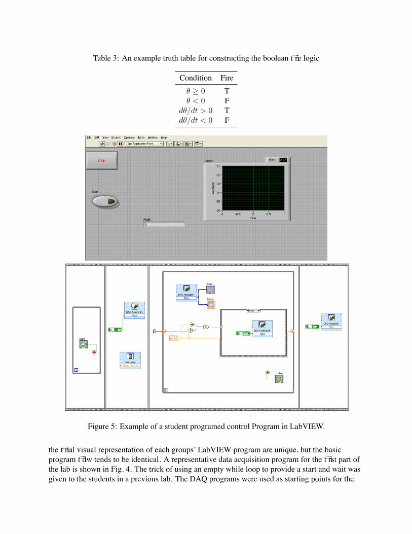
Table 3: An example truth table for constructing the boolean fire logic

Condition Fireθ ≥ 0 Tθ < 0 F

dθ/dt > 0 Tdθ/dt < 0 F

Figure 5: Example of a student programed control Program in LabVIEW.

the final visual representation of each groups’ LabVIEW program are unique, but the basicprogram flow tends to be identical. A representative data acquisition program for the first part ofthe lab is shown in Fig. 4. The trick of using an empty while loop to provide a start and wait wasgiven to the students in a previous lab. The DAQ programs were used as starting points for the

control systems. Students typically removed the unnecessary acquisition tasks and thenimplemented the control system. Boolean logic blocks were used to test the position constraints,with the differential constraint being implemented through a simple shift register. Students weregiven help as required with specific implementation questions (i.e. where is the shift registerfound?) if needed. An example of a student implemented control program is shown in Fig. 6.

Figure 6: Example of a student programed control Program in LabVIEW.

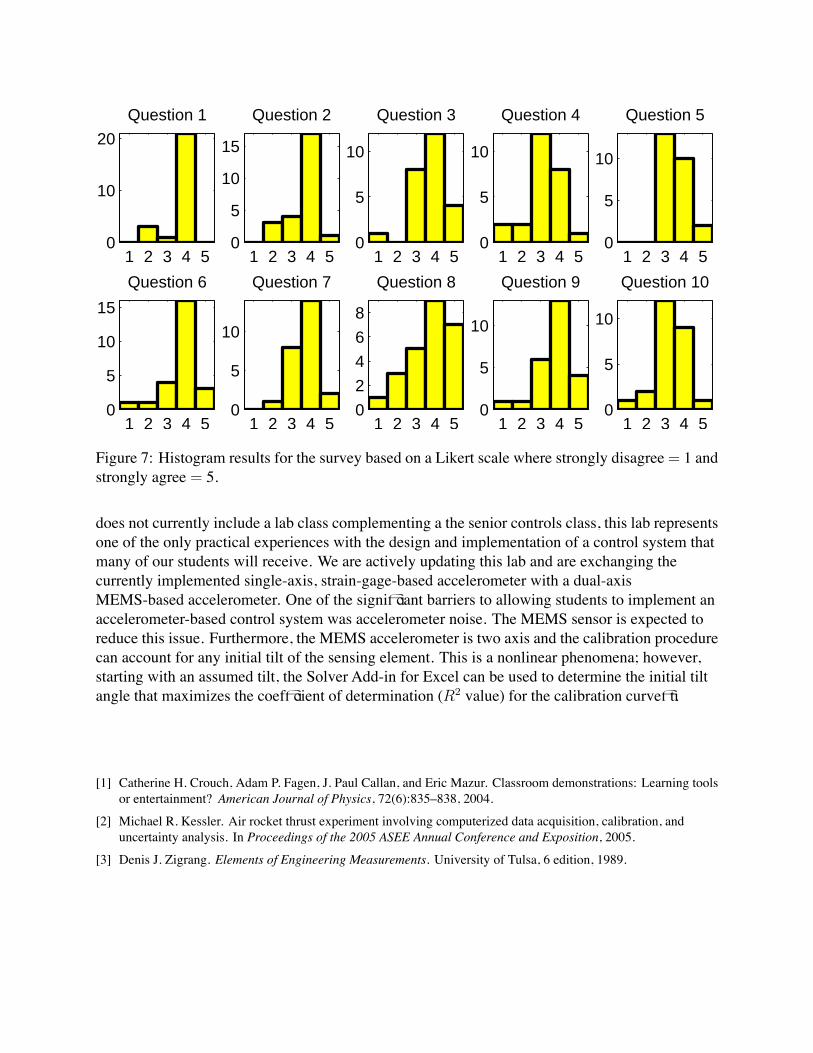
Student AssessmentStudents were given a 9 question survey to assess the effectiveness of the educational objectivesof the lab. Questions pertaining to the instrumentation and experimental analysis objective andthe introduction to control systems objective were included in the survey. The questionnaire was a5 point Likert-type survey asking each student to indicate if they strongly disagree, disagree,neither agree nor disagree, agree, or strongly agree. The last question was an open response

asking for comments about the lab either in criticism or appreciation. The Likert scaled questionsand average value of the responses are listed in Table 4. Histograms of the response for eachquestion are shown in Figure 7.

Table 4: Likert Scale survey question

Question Average Response1. The experiment did a good job of familiarizing me with typical instrumentcalibration procedures.

3.72

2. The laboratory did a good job of familiarizing me with computerized dataacquisition.

3.64

3. The laboratory did a good job of familiarizing me with the operation of arotary encoder, strain gages, accelerometer, and pressure transducer.

3.72

4. Detailed uncertainty analysis became clearer as a result of the experimentand lab write-up.

3.16

5. The lab and subsequent lab report caused me to think critically aboutsources of experimental error that contribute to uncertainty in the rocket en-gine thrust.

3.58

6. The lab did a good job introducing me to the concepts of control systems. 3.767. My understanding of how data acquisition and control systems work to-gether was improved.

3.68

8. Overall the lab was a positive experience. 3.729. Overall the lab helped me learn and understand experiments. 3.7210. Overall the lab write-up was a positive experience. 3.28

In general, the students felt that the lab was a good introduction to control systems as indicated bythe results of question 6. The students also generally agreed that the lab was a good introductionto calibration and computer-based data acquisition. Only limited responses were collected fromthe open-ended question. The control system portion of the lab was generally considered a goodintroduction to feedback control systems. The students also felt that the lab successfullydemonstrated the relationship between data acquisition systems and control systems.ConclusionsA lab was designed that enabled an open ended experience with the implementation and analysisof an experiment. This lab was the culmination of a series of directed experiments and gavestudents an experience in constructing and implementing an experiment from start to finish. Therequirement to develop a basic control system also introduced the students to the design andimplementation of a feedback control system. Students successfully implemented acondition-based firing scheme that took feedback from sensors and determined a firing time. Ingeneral, the students responded that the lab was a good introduction to control systems based on apost-lab survey.Future PlansThis lab is under continuous improvement. The results in this paper represent the first completeimplementation of the full data acquisition lab and the control system lab. Since our curriculum

1 2 3 4 50

10

20

Question 1

1 2 3 4 50

5

10

15

Question 2

1 2 3 4 50

5

10

Question 3

1 2 3 4 50

5

10

Question 4

1 2 3 4 50

5

10

Question 5

1 2 3 4 50

5

10

15

Question 6

1 2 3 4 50

5

10

Question 7

1 2 3 4 50

2

4

6

8

Question 8

1 2 3 4 50

5

10

Question 9

1 2 3 4 50

5

10

Question 10

Figure 7: Histogram results for the survey based on a Likert scale where strongly disagree = 1 andstrongly agree = 5.

does not currently include a lab class complementing a the senior controls class, this lab representsone of the only practical experiences with the design and implementation of a control system thatmany of our students will receive. We are actively updating this lab and are exchanging thecurrently implemented single-axis, strain-gage-based accelerometer with a dual-axisMEMS-based accelerometer. One of the significant barriers to allowing students to implement anaccelerometer-based control system was accelerometer noise. The MEMS sensor is expected toreduce this issue. Furthermore, the MEMS accelerometer is two axis and the calibration procedurecan account for any initial tilt of the sensing element. This is a nonlinear phenomena; however,starting with an assumed tilt, the Solver Add-in for Excel can be used to determine the initial tiltangle that maximizes the coefficient of determination (R2 value) for the calibration curvefit.

[1] Catherine H. Crouch, Adam P. Fagen, J. Paul Callan, and Eric Mazur. Classroom demonstrations: Learning toolsor entertainment? American Journal of Physics, 72(6):835–838, 2004.

[2] Michael R. Kessler. Air rocket thrust experiment involving computerized data acquisition, calibration, anduncertainty analysis. In Proceedings of the 2005 ASEE Annual Conference and Exposition, 2005.

[3] Denis J. Zigrang. Elements of Engineering Measurements. University of Tulsa, 6 edition, 1989.