introduction to high performance computing forprdrklaina.weebly.com/uploads/5/7/7/3/5773421/... ·...
TRANSCRIPT


Introduction to High Performance
Computing for Scientists and Engineers
K10600_FM.indd 1 6/1/10 11:51:56 AM

Chapman & Hall/CRC Computational Science Series
PETASCALE COMPUTING: ALGORITHMS AND APPLICATIONSEdited by David A. Bader
PROCESS ALGEBRA FOR PARALLEL AND DISTRIBUTED PROCESSINGEdited by Michael Alexander and William Gardner
GRID COMPUTING: TECHNIQUES AND APPLICATIONSBarry Wilkinson
INTRODUCTION TO CONCURRENCY IN PROGRAMMING LANGUAGESMatthew J. Sottile, Timothy G. Mattson, and Craig E Rasmussen
INTRODUCTION TO SCHEDULINGYves Robert and Frédéric Vivien
SCIENTIFIC DATA MANAGEMENT: CHALLENGES, TECHNOLOGY, AND DEPLOYMENTEdited by Arie Shoshani and Doron Rotem
INTRODUCTION TO THE SIMULATION OF DYNAMICS USING SIMULINK®
Michael A. Gray
INTRODUCTION TO HIGH PERFORMANCE COMPUTING FOR SCIENTISTS AND ENGINEERS, Georg Hager and Gerhard Wellein
PUBLISHED TITLES
SERIES EDITOR
Horst SimonAssociate Laboratory Director, Computing Sciences
Lawrence Berkeley National Laboratory
Berkeley, California, U.S.A.
AIMS AND SCOPE
This series aims to capture new developments and applications in the field of computational sci-ence through the publication of a broad range of textbooks, reference works, and handbooks. Books in this series will provide introductory as well as advanced material on mathematical, sta-tistical, and computational methods and techniques, and will present researchers with the latest theories and experimentation. The scope of the series includes, but is not limited to, titles in the areas of scientific computing, parallel and distributed computing, high performance computing, grid computing, cluster computing, heterogeneous computing, quantum computing, and their applications in scientific disciplines such as astrophysics, aeronautics, biology, chemistry, climate modeling, combustion, cosmology, earthquake prediction, imaging, materials, neuroscience, oil exploration, and weather forecasting.
Introduction to High Performance
Computing for Scientists and Engineers
Georg Hager
Gerhard Wellein
K10600_FM.indd 2 6/1/10 11:51:56 AM

Chapman & Hall/CRC Computational Science Series
PETASCALE COMPUTING: ALGORITHMS AND APPLICATIONSEdited by David A. Bader
PROCESS ALGEBRA FOR PARALLEL AND DISTRIBUTED PROCESSINGEdited by Michael Alexander and William Gardner
GRID COMPUTING: TECHNIQUES AND APPLICATIONSBarry Wilkinson
INTRODUCTION TO CONCURRENCY IN PROGRAMMING LANGUAGESMatthew J. Sottile, Timothy G. Mattson, and Craig E Rasmussen
INTRODUCTION TO SCHEDULINGYves Robert and Frédéric Vivien
SCIENTIFIC DATA MANAGEMENT: CHALLENGES, TECHNOLOGY, AND DEPLOYMENTEdited by Arie Shoshani and Doron Rotem
INTRODUCTION TO THE SIMULATION OF DYNAMICS USING SIMULINK®
Michael A. Gray
INTRODUCTION TO HIGH PERFORMANCE COMPUTING FOR SCIENTISTS AND ENGINEERS, Georg Hager and Gerhard Wellein
PUBLISHED TITLES
SERIES EDITOR
Horst SimonAssociate Laboratory Director, Computing Sciences
Lawrence Berkeley National Laboratory
Berkeley, California, U.S.A.
AIMS AND SCOPE
This series aims to capture new developments and applications in the field of computational sci-ence through the publication of a broad range of textbooks, reference works, and handbooks. Books in this series will provide introductory as well as advanced material on mathematical, sta-tistical, and computational methods and techniques, and will present researchers with the latest theories and experimentation. The scope of the series includes, but is not limited to, titles in the areas of scientific computing, parallel and distributed computing, high performance computing, grid computing, cluster computing, heterogeneous computing, quantum computing, and their applications in scientific disciplines such as astrophysics, aeronautics, biology, chemistry, climate modeling, combustion, cosmology, earthquake prediction, imaging, materials, neuroscience, oil exploration, and weather forecasting.
Introduction to High Performance
Computing for Scientists and Engineers
Georg Hager
Gerhard Wellein
K10600_FM.indd 3 6/1/10 11:51:57 AM

CRC PressTaylor & Francis Group6000 Broken Sound Parkway NW, Suite 300Boca Raton, FL 33487-2742
© 2011 by Taylor and Francis Group, LLCCRC Press is an imprint of Taylor & Francis Group, an Informa business
No claim to original U.S. Government works
Printed in the United States of America on acid-free paper10 9 8 7 6 5 4 3 2 1
International Standard Book Number: 978-1-4398-1192-4 (Paperback)
This book contains information obtained from authentic and highly regarded sources. Reasonable efforts have been made to publish reliable data and information, but the author and publisher cannot assume responsibility for the validity of all materials or the consequences of their use. The authors and publishers have attempted to trace the copyright holders of all material reproduced in this publication and apologize to copyright holders if permission to publish in this form has not been obtained. If any copyright material has not been acknowledged please write and let us know so we may rectify in any future reprint.
Except as permitted under U.S. Copyright Law, no part of this book may be reprinted, reproduced, transmit-ted, or utilized in any form by any electronic, mechanical, or other means, now known or hereafter invented, including photocopying, microfilming, and recording, or in any information storage or retrieval system, without written permission from the publishers.
For permission to photocopy or use material electronically from this work, please access www.copyright.com (http://www.copyright.com/) or contact the Copyright Clearance Center, Inc. (CCC), 222 Rosewood Drive, Danvers, MA 01923, 978-750-8400. CCC is a not-for-profit organization that provides licenses and registration for a variety of users. For organizations that have been granted a photocopy license by the CCC, a separate system of payment has been arranged.
Trademark Notice: Product or corporate names may be trademarks or registered trademarks, and are used only for identification and explanation without intent to infringe.
Library of Congress Cataloging‑in‑Publication Data
Hager, Georg.Introduction to high performance computing for scientists and engineers / Georg
Hager and Gerhard Wellein.p. cm. -- (Chapman & Hall/CRC computational science series ; 7)
Includes bibliographical references and index.ISBN 978-1-4398-1192-4 (alk. paper)1. High performance computing. I. Wellein, Gerhard. II. Title.
QA76.88.H34 2011004’.35--dc22 2010009624
Visit the Taylor & Francis Web site athttp://www.taylorandfrancis.com
and the CRC Press Web site athttp://www.crcpress.com
K10600_FM.indd 4 6/1/10 11:51:57 AM

Dedicated to Konrad Zuse (1910–1995)
He developed and built the world’s first fully automated, freely programmablecomputer with binary floating-point arithmetic in 1941.

Contents
Foreword xiii
Preface xv
About the authors xxi
List of acronyms and abbreviations xxiii
1 Modern processors 1
1.1 Stored-program computer architecture . . . . . . . . . . . . . . . . 11.2 General-purpose cache-based microprocessor architecture . . . . . 2
1.2.1 Performance metrics and benchmarks . . . . . . . . . . . . 31.2.2 Transistors galore: Moore’s Law . . . . . . . . . . . . . . . 71.2.3 Pipelining . . . . . . . . . . . . . . . . . . . . . . . . . . . 91.2.4 Superscalarity . . . . . . . . . . . . . . . . . . . . . . . . . 131.2.5 SIMD . . . . . . . . . . . . . . . . . . . . . . . . . . . . . 14
1.3 Memory hierarchies . . . . . . . . . . . . . . . . . . . . . . . . . 151.3.1 Cache . . . . . . . . . . . . . . . . . . . . . . . . . . . . . 151.3.2 Cache mapping . . . . . . . . . . . . . . . . . . . . . . . . 181.3.3 Prefetch . . . . . . . . . . . . . . . . . . . . . . . . . . . . 20
1.4 Multicore processors . . . . . . . . . . . . . . . . . . . . . . . . . 231.5 Multithreaded processors . . . . . . . . . . . . . . . . . . . . . . . 261.6 Vector processors . . . . . . . . . . . . . . . . . . . . . . . . . . . 28
1.6.1 Design principles . . . . . . . . . . . . . . . . . . . . . . . 291.6.2 Maximum performance estimates . . . . . . . . . . . . . . 311.6.3 Programming for vector architectures . . . . . . . . . . . . 32
2 Basic optimization techniques for serial code 37
2.1 Scalar profiling . . . . . . . . . . . . . . . . . . . . . . . . . . . . 372.1.1 Function- and line-based runtime profiling . . . . . . . . . . 382.1.2 Hardware performance counters . . . . . . . . . . . . . . . 412.1.3 Manual instrumentation . . . . . . . . . . . . . . . . . . . 45
2.2 Common sense optimizations . . . . . . . . . . . . . . . . . . . . 452.2.1 Do less work! . . . . . . . . . . . . . . . . . . . . . . . . . 452.2.2 Avoid expensive operations! . . . . . . . . . . . . . . . . . 462.2.3 Shrink the working set! . . . . . . . . . . . . . . . . . . . . 47
vii

viii
2.3 Simple measures, large impact . . . . . . . . . . . . . . . . . . . . 472.3.1 Elimination of common subexpressions . . . . . . . . . . . 472.3.2 Avoiding branches . . . . . . . . . . . . . . . . . . . . . . 482.3.3 Using SIMD instruction sets . . . . . . . . . . . . . . . . . 49
2.4 The role of compilers . . . . . . . . . . . . . . . . . . . . . . . . . 512.4.1 General optimization options . . . . . . . . . . . . . . . . . 522.4.2 Inlining . . . . . . . . . . . . . . . . . . . . . . . . . . . . 522.4.3 Aliasing . . . . . . . . . . . . . . . . . . . . . . . . . . . . 532.4.4 Computational accuracy . . . . . . . . . . . . . . . . . . . 542.4.5 Register optimizations . . . . . . . . . . . . . . . . . . . . 552.4.6 Using compiler logs . . . . . . . . . . . . . . . . . . . . . 55
2.5 C++ optimizations . . . . . . . . . . . . . . . . . . . . . . . . . . 562.5.1 Temporaries . . . . . . . . . . . . . . . . . . . . . . . . . . 562.5.2 Dynamic memory management . . . . . . . . . . . . . . . 592.5.3 Loop kernels and iterators . . . . . . . . . . . . . . . . . . 60
3 Data access optimization 63
3.1 Balance analysis and lightspeed estimates . . . . . . . . . . . . . . 633.1.1 Bandwidth-based performance modeling . . . . . . . . . . 633.1.2 The STREAM benchmarks . . . . . . . . . . . . . . . . . . 67
3.2 Storage order . . . . . . . . . . . . . . . . . . . . . . . . . . . . . 693.3 Case study: The Jacobi algorithm . . . . . . . . . . . . . . . . . . 713.4 Case study: Dense matrix transpose . . . . . . . . . . . . . . . . . 743.5 Algorithm classification and access optimizations . . . . . . . . . . 79
3.5.1 O(N)/O(N) . . . . . . . . . . . . . . . . . . . . . . . . . . 793.5.2 O(N2)/O(N2) . . . . . . . . . . . . . . . . . . . . . . . . 793.5.3 O(N3)/O(N2) . . . . . . . . . . . . . . . . . . . . . . . . 84
3.6 Case study: Sparse matrix-vector multiply . . . . . . . . . . . . . . 863.6.1 Sparse matrix storage schemes . . . . . . . . . . . . . . . . 863.6.2 Optimizing JDS sparse MVM . . . . . . . . . . . . . . . . 89
4 Parallel computers 95
4.1 Taxonomy of parallel computing paradigms . . . . . . . . . . . . . 964.2 Shared-memory computers . . . . . . . . . . . . . . . . . . . . . . 97
4.2.1 Cache coherence . . . . . . . . . . . . . . . . . . . . . . . 974.2.2 UMA . . . . . . . . . . . . . . . . . . . . . . . . . . . . . 994.2.3 ccNUMA . . . . . . . . . . . . . . . . . . . . . . . . . . . 100
4.3 Distributed-memory computers . . . . . . . . . . . . . . . . . . . 1024.4 Hierarchical (hybrid) systems . . . . . . . . . . . . . . . . . . . . 1034.5 Networks . . . . . . . . . . . . . . . . . . . . . . . . . . . . . . . 104
4.5.1 Basic performance characteristics of networks . . . . . . . . 1044.5.2 Buses . . . . . . . . . . . . . . . . . . . . . . . . . . . . . 1094.5.3 Switched and fat-tree networks . . . . . . . . . . . . . . . . 1104.5.4 Mesh networks . . . . . . . . . . . . . . . . . . . . . . . . 1124.5.5 Hybrids . . . . . . . . . . . . . . . . . . . . . . . . . . . . 113

ix
5 Basics of parallelization 115
5.1 Why parallelize? . . . . . . . . . . . . . . . . . . . . . . . . . . . 1155.2 Parallelism . . . . . . . . . . . . . . . . . . . . . . . . . . . . . . 116
5.2.1 Data parallelism . . . . . . . . . . . . . . . . . . . . . . . 1165.2.2 Functional parallelism . . . . . . . . . . . . . . . . . . . . 119
5.3 Parallel scalability . . . . . . . . . . . . . . . . . . . . . . . . . . 1205.3.1 Factors that limit parallel execution . . . . . . . . . . . . . 1205.3.2 Scalability metrics . . . . . . . . . . . . . . . . . . . . . . 1225.3.3 Simple scalability laws . . . . . . . . . . . . . . . . . . . . 1235.3.4 Parallel efficiency . . . . . . . . . . . . . . . . . . . . . . . 1255.3.5 Serial performance versus strong scalability . . . . . . . . . 1265.3.6 Refined performance models . . . . . . . . . . . . . . . . . 1285.3.7 Choosing the right scaling baseline . . . . . . . . . . . . . 1305.3.8 Case study: Can slower processors compute faster? . . . . . 1315.3.9 Load imbalance . . . . . . . . . . . . . . . . . . . . . . . . 137
6 Shared-memory parallel programming with OpenMP 143
6.1 Short introduction to OpenMP . . . . . . . . . . . . . . . . . . . . 1436.1.1 Parallel execution . . . . . . . . . . . . . . . . . . . . . . . 1446.1.2 Data scoping . . . . . . . . . . . . . . . . . . . . . . . . . 1466.1.3 OpenMP worksharing for loops . . . . . . . . . . . . . . . 1476.1.4 Synchronization . . . . . . . . . . . . . . . . . . . . . . . 1496.1.5 Reductions . . . . . . . . . . . . . . . . . . . . . . . . . . 1506.1.6 Loop scheduling . . . . . . . . . . . . . . . . . . . . . . . 1516.1.7 Tasking . . . . . . . . . . . . . . . . . . . . . . . . . . . . 1536.1.8 Miscellaneous . . . . . . . . . . . . . . . . . . . . . . . . 154
6.2 Case study: OpenMP-parallel Jacobi algorithm . . . . . . . . . . . 1566.3 Advanced OpenMP: Wavefront parallelization . . . . . . . . . . . 158
7 Efficient OpenMP programming 165
7.1 Profiling OpenMP programs . . . . . . . . . . . . . . . . . . . . . 1657.2 Performance pitfalls . . . . . . . . . . . . . . . . . . . . . . . . . 166
7.2.1 Ameliorating the impact of OpenMP worksharing constructs 1687.2.2 Determining OpenMP overhead for short loops . . . . . . . 1757.2.3 Serialization . . . . . . . . . . . . . . . . . . . . . . . . . 1777.2.4 False sharing . . . . . . . . . . . . . . . . . . . . . . . . . 179
7.3 Case study: Parallel sparse matrix-vector multiply . . . . . . . . . 181
8 Locality optimizations on ccNUMA architectures 185
8.1 Locality of access on ccNUMA . . . . . . . . . . . . . . . . . . . 1858.1.1 Page placement by first touch . . . . . . . . . . . . . . . . 1868.1.2 Access locality by other means . . . . . . . . . . . . . . . . 190
8.2 Case study: ccNUMA optimization of sparse MVM . . . . . . . . 1908.3 Placement pitfalls . . . . . . . . . . . . . . . . . . . . . . . . . . . 192
8.3.1 NUMA-unfriendly OpenMP scheduling . . . . . . . . . . . 192

x
8.3.2 File system cache . . . . . . . . . . . . . . . . . . . . . . . 1948.4 ccNUMA issues with C++ . . . . . . . . . . . . . . . . . . . . . . 197
8.4.1 Arrays of objects . . . . . . . . . . . . . . . . . . . . . . . 1978.4.2 Standard Template Library . . . . . . . . . . . . . . . . . . 199
9 Distributed-memory parallel programming with MPI 203
9.1 Message passing . . . . . . . . . . . . . . . . . . . . . . . . . . . 2039.2 A short introduction to MPI . . . . . . . . . . . . . . . . . . . . . 205
9.2.1 A simple example . . . . . . . . . . . . . . . . . . . . . . 2059.2.2 Messages and point-to-point communication . . . . . . . . 2079.2.3 Collective communication . . . . . . . . . . . . . . . . . . 2139.2.4 Nonblocking point-to-point communication . . . . . . . . . 2169.2.5 Virtual topologies . . . . . . . . . . . . . . . . . . . . . . . 220
9.3 Example: MPI parallelization of a Jacobi solver . . . . . . . . . . . 2249.3.1 MPI implementation . . . . . . . . . . . . . . . . . . . . . 2249.3.2 Performance properties . . . . . . . . . . . . . . . . . . . . 230
10 Efficient MPI programming 235
10.1 MPI performance tools . . . . . . . . . . . . . . . . . . . . . . . . 23510.2 Communication parameters . . . . . . . . . . . . . . . . . . . . . 23910.3 Synchronization, serialization, contention . . . . . . . . . . . . . . 240
10.3.1 Implicit serialization and synchronization . . . . . . . . . . 24010.3.2 Contention . . . . . . . . . . . . . . . . . . . . . . . . . . 243
10.4 Reducing communication overhead . . . . . . . . . . . . . . . . . 24410.4.1 Optimal domain decomposition . . . . . . . . . . . . . . . 24410.4.2 Aggregating messages . . . . . . . . . . . . . . . . . . . . 24810.4.3 Nonblocking vs. asynchronous communication . . . . . . . 25010.4.4 Collective communication . . . . . . . . . . . . . . . . . . 253
10.5 Understanding intranode point-to-point communication . . . . . . . 253
11 Hybrid parallelization with MPI and OpenMP 263
11.1 Basic MPI/OpenMP programming models . . . . . . . . . . . . . 26411.1.1 Vector mode implementation . . . . . . . . . . . . . . . . . 26411.1.2 Task mode implementation . . . . . . . . . . . . . . . . . . 26511.1.3 Case study: Hybrid Jacobi solver . . . . . . . . . . . . . . . 267
11.2 MPI taxonomy of thread interoperability . . . . . . . . . . . . . . 26811.3 Hybrid decomposition and mapping . . . . . . . . . . . . . . . . . 27011.4 Potential benefits and drawbacks of hybrid programming . . . . . . 273
A Topology and affinity in multicore environments 277
A.1 Topology . . . . . . . . . . . . . . . . . . . . . . . . . . . . . . . 279A.2 Thread and process placement . . . . . . . . . . . . . . . . . . . . 280
A.2.1 External affinity control . . . . . . . . . . . . . . . . . . . 280A.2.2 Affinity under program control . . . . . . . . . . . . . . . . 283
A.3 Page placement beyond first touch . . . . . . . . . . . . . . . . . . 284

xi
B Solutions to the problems 287
Bibliography 309
Index 323

This page intentionally left blank.
Foreword
Georg Hager and Gerhard Wellein have developed a very approachable introductionto high performance computing for scientists and engineers. Their style and descrip-tions are easy to read and follow.
The idea that computational modeling and simulation represent a new branch ofscientific methodology, alongside theory and experimentation, was introduced abouttwo decades ago. It has since come to symbolize the enthusiasm and sense of im-portance that people in our community feel for the work they are doing. Many of ustoday want to hasten that growth and believe that the most progressive steps in that di-rection require much more understanding of the vital core of computational science:software and the mathematical models and algorithms it encodes. Of course, thegeneral and widespread obsession with hardware is understandable, especially givenexponential increases in processor performance, the constant evolution of processorarchitectures and supercomputer designs, and the natural fascination that people havefor big, fast machines. But when it comes to advancing the cause of computationalmodeling and simulation as a new part of the scientific method there is no doubt thatthe complex software “ecosystem” it requires must take its place on the center stage.
At the application level science has to be captured in mathematical models, whichin turn are expressed algorithmically and ultimately encoded as software. Accord-ingly, on typical projects the majority of the funding goes to support this translationprocess that starts with scientific ideas and ends with executable software, and whichover its course requires intimate collaboration among domain scientists, computerscientists, and applied mathematicians. This process also relies on a large infrastruc-ture of mathematical libraries, protocols, and system software that has taken years tobuild up and that must be maintained, ported, and enhanced for many years to come ifthe value of the application codes that depend on it are to be preserved and extended.The software that encapsulates all this time, energy, and thought routinely outlasts(usually by years, sometimes by decades) the hardware it was originally designed torun on, as well as the individuals who designed and developed it.
This book covers the basics of modern processor architecture and serial optimiza-tion techniques that can effectively exploit the architectural features for scientificcomputing. The authors provide a discussion of the critical issues in data movementand illustrate this with examples. A number of central issues in high performancecomputing are discussed at a level that is easily understandable. The use of parallelprocessing in shared, nonuniform access, and distributed memories is discussed. Inaddition the popular programming styles of OpenMP, MPI and mixed programmingare highlighted.
xiii

xiv
We live in an exciting time in the use of high performance computing and a pe-riod that promises unmatched performance for those who can effectively utilize thesystems for high performance computing. This book presents a balanced treatment ofthe theory, technology, architecture, and software for modern high performance com-puters and the use of high performance computing systems. The focus on scientificand engineering problems makes it both educational and unique. I highly recom-mend this timely book for scientists and engineers, and I believe it will benefit manyreaders and provide a fine reference.
Jack Dongarra
University of TennesseeKnoxville, Tennessee
USA
Preface
When Konrad Zuse constructed the world’s first fully automated, freely pro-grammable computer with binary floating-point arithmetic in 1941 [H129], he hadgreat visions regarding the possible use of his revolutionary device, not only in sci-ence and engineering but in all sectors of life [H130]. Today, his dream is reality:Computing in all its facets has radically changed the way we live and perform re-search since Zuse’s days. Computers have become essential due to their ability toperform calculations, visualizations, and general data processing at an incredible,ever-increasing speed. They allow us to offload daunting routine tasks and commu-nicate without delay.
Science and engineering have profited in a special way from this development.It was recognized very early that computers can help tackle problems that were for-merly too computationally challenging, or perform virtual experiments that wouldbe too complex, expensive, or outright dangerous to carry out in reality. Computa-
tional fluid dynamics, or CFD, is a typical example: The simulation of fluid flow inarbitrary geometries is a standard task. No airplane, no car, no high-speed train, noturbine bucket enters manufacturing without prior CFD analysis. This does not meanthat the days of wind tunnels and wooden mock-ups are numbered, but that com-puter simulation supports research and engineering as a third pillar beside theory andexperiment, not only on fluid dynamics but nearly all other fields of science. In re-cent years, pharmaceutical drug design has emerged as a thrilling new applicationarea for fast computers. Software enables chemists to discover reaction mechanismsliterally at the click of their mouse, simulating the complex dynamics of the largemolecules that govern the inner mechanics of life. On even smaller scales, theoreti-
cal solid state physics explores the structure of solids by modeling the interactions oftheir constituents, nuclei and electrons, on the quantum level [A79], where the sheernumber of degrees of freedom rules out any analytical treatment in certain limits andrequires vast computational resources. The list goes on and on: Quantum chromody-namics, materials science, structural mechanics, and medical image processing arejust a few further application areas.
Computer-based simulations have become ubiquitous standard tools, and are in-dispensable for most research areas both in academia and industry. Although thepower of the PC has brought many of those computational chores to the researcher’sdesktop, there was, still is and probably will ever be this special group of peoplewhose requirements on storage, main memory, or raw computational speed cannotbe met by a single desktop machine. High performance parallel computers come totheir rescue.
xv

xvi
Employing high performance computing (HPC) as a research tool demands atleast a basic understanding of the hardware concepts and software issues involved.This is already true when only using turnkey application software, but it becomesessential if code development is required. However, in all our years of teaching andworking with scientists and engineers we have learned that such knowledge is volatile
— in the sense that it is hard to establish and maintain an adequate competence levelwithin the different research groups. The new PhD student is all too often left alonewith the steep learning curve of HPC, but who is to blame? After all, the goal ofresearch and development is to make scientific progress, for which HPC is just atool. It is essential, sometimes unwieldy, and always expensive, but it is still a tool.Nevertheless, writing efficient and parallel code is the admission ticket to high per-formance computing, which was for a long time an exquisite and small world. Tech-nological changes have brought parallel computing first to the departmental level andrecently even to the desktop. In times of stagnating single processor capabilities andincreasing parallelism, a growing audience of scientists and engineers must be con-cerned with performance and scalability. These are the topics we are aiming at withthis book, and the reason we wrote it was to make the knowledge about them lessvolatile.
Actually, a lot of good literature exists on all aspects of computer architecture,optimization, and HPC [S1, R34, S2, S3, S4]. Although the basic principles haven’tchanged much, a lot of it is outdated at the time of writing: We have seen the declineof vector computers (and also of one or the other highly promising microprocessordesign), ubiquitous SIMD capabilities, the advent of multicore processors, the grow-ing presence of ccNUMA, and the introduction of cost-effective high-performanceinterconnects. Perhaps the most striking development is the absolute dominance ofx86-based commodity clusters running the Linux OS on Intel or AMD processors.Recent publications are often focused on very specific aspects, and are unsuitablefor the student or the scientist who wants to get a fast overview and maybe later diveinto the details. Our goal is to provide a solid introduction to the architecture and pro-gramming of high performance computers, with an emphasis on performance issues.In our experience, users all too often have no idea what factors limit time to solution,and whether it makes sense to think about optimization at all. Readers of this bookwill get an intuitive understanding of performance limitations without much com-puter science ballast, to a level of knowledge that enables them to understand morespecialized sources. To this end we have compiled an extensive bibliography, whichis also available online in a hyperlinked and commented version at the book’s Website: http://www.hpc.rrze.uni-erlangen.de/HPC4SE/.
Who this book is for
We believe that working in a scientific computing center gave us a unique viewof the requirements and attitudes of users as well as manufacturers of parallel com-puters. Therefore, everybody who has to deal with high performance computing may

xvii
profit from this book: Students and teachers of computer science, computational en-gineering, or any field even marginally concerned with simulation may use it as anaccompanying textbook. For scientists and engineers who must get a quick grasp ofHPC basics it can be a starting point to prepare for more advanced literature. Andfinally, professional cluster builders can definitely use the knowledge we convey toprovide a better service to their customers. The reader should have some familiaritywith programming and high-level computer architecture. Even so, we must empha-size that it is an introduction rather than an exhaustive reference; the Encyclopedia
of High Performance Computing has yet to be written.
What’s in this book, and what’s not
High performance computing as we understand it deals with the implementations
of given algorithms (also commonly referred to as “code”), and the hardware theyrun on. We assume that someone who wants to use HPC resources is already awareof the different algorithms that can be used to tackle their problem, and we makeno attempt to provide alternatives. Of course we have to pick certain examples inorder to get the point across, but it is always understood that there may be other, andprobably more adequate algorithms. The reader is then expected to use the strategieslearned from our examples.
Although we tried to keep the book concise, the temptation to cover everything isoverwhelming. However, we deliberately (almost) ignore very recent developmentslike modern accelerator technologies (GPGPU, FPGA, Cell processor), mostly be-cause they are so much in a state of flux that coverage with any claim of depth wouldbe almost instantly outdated. One may also argue that high performance input/out-put should belong in an HPC book, but we think that efficient parallel I/O is anadvanced and highly system-dependent topic, which is best treated elsewhere. Onthe software side we concentrate on basic sequential optimization strategies and thedominating parallelization paradigms: shared-memory parallelization with OpenMPand distributed-memory parallel programming with MPI. Alternatives like UnifiedParallel C (UPC), Co-Array Fortran (CAF), or other, more modern approaches stillhave to prove their potential for getting at least as efficient, and thus accepted, asMPI and OpenMP.
Most concepts are presented on a level independent of specific architectures,although we cannot ignore the dominating presence of commodity systems. Thus,when we show case studies and actual performance numbers, those have usually beenobtained on x86-based clusters with standard interconnects. Almost all code exam-ples are in Fortran; we switch to C or C++ only if the peculiarities of those languagesare relevant in a certain setting. Some of the codes used for producing benchmarkresults are available for download at the book’s Web site: http://www.hpc.rrze.uni-
erlangen.de/HPC4SE/.This book is organized as follows: In Chapter 1 we introduce the architecture of
modern cache-based microprocessors and discuss their inherent performance limi-
xviii
tations. Recent developments like multicore chips and simultaneous multithreading(SMT) receive due attention. Vector processors are briefly touched, although theyhave all but vanished from the HPC market. Chapters 2 and 3 describe general opti-mization strategies for serial code on cache-based architectures. Simple models areused to convey the concept of “best possible” performance of loop kernels, and weshow how to raise those limits by code transformations. Actually, we believe thatperformance modeling of applications on all levels of a system’s architecture is ofutmost importance, and we regard it as an indispensable guiding principle in HPC.
In Chapter 4 we turn to parallel computer architectures of the shared-memory andthe distributed-memory type, and also cover the most relevant network topologies.Chapter 5 then covers parallel computing on a theoretical level: Starting with someimportant parallel programming patterns, we turn to performance models that ex-plain the limitations on parallel scalability. The questions why and when it can makesense to build massively parallel systems with “slow” processors are answered alongthe way. Chapter 6 gives a brief introduction to OpenMP, which is still the dominat-ing parallelization paradigm on shared-memory systems for scientific applications.Chapter 7 deals with some typical performance problems connected with OpenMPand shows how to avoid or ameliorate them. Since cache-coherent nonuniform mem-ory access (ccNUMA) systems have proliferated the commodity HPC market (a factthat is still widely ignored even by some HPC “professionals”), we dedicate Chap-ter 8 to ccNUMA-specific optimization techniques. Chapters 9 and 10 are concernedwith distributed-memory parallel programming with the Message Passing Interface(MPI), and writing efficient MPI code. Finally, Chapter 11 gives an introduction tohybrid programming with MPI and OpenMP combined. Every chapter closes witha set of problems, which we highly recommend to all readers. The problems fre-quently cover “odds and ends” that somehow did not fit somewhere else, or elaborateon special topics. Solutions are provided in Appendix B.
We certainly recommend reading the book cover to cover, because there is not asingle topic that we consider “less important.” However, readers who are interestedin OpenMP and MPI alone can easily start off with Chapters 6 and 9 for the basicinformation, and then dive into the corresponding optimization chapters (7, 8, and10). The text is heavily cross-referenced, so it should be easy to collect the missingbits and pieces from other parts of the book.
Acknowledgments
This book originated from a two-chapter contribution to a Springer “LectureNotes in Physics” volume, which comprised the proceedings of a 2006 summerschool on computational many-particle physics [A79]. We thank the organizers ofthis workshop, notably Holger Fehske, Ralf Schneider, and Alexander Weisse, formaking us put down our HPC experience for the first time in coherent form. Al-though we extended the material considerably, we would most probably never havewritten a book without this initial seed.

xix
Over a decade of working with users, students, algorithms, codes, and tools wentinto these pages. Many people have thus contributed, directly or indirectly, and some-times unknowingly. In particular we have to thank the staff of HPC Services at Er-langen Regional Computing Center (RRZE), especially Thomas Zeiser, Jan Treibig,Michael Meier, Markus Wittmann, Johannes Habich, Gerald Schubert, and HolgerStengel, for countless lively discussions leading to invaluable insights. Over the lastdecade the group has continuously received financial support by the “CompetenceNetwork for Scientific High Performance Computing in Bavaria” (KONWIHR) andthe Friedrich-Alexander University of Erlangen-Nuremberg. Both bodies shared ourvision of HPC as an indispensable tool for many scientists and engineers.
We are also indebted to Uwe Küster (HLRS Stuttgart), Matthias Müller (ZIHDresden), Reinhold Bader, and Matthias Brehm (both LRZ München), for a highlyefficient cooperation between our centers, which enabled many activities and col-laborations. Special thanks goes to Darren Kerbyson (PNNL) for his encouragementand many astute comments on our work. Last, but not least, we want to thank RolfRabenseifner (HLRS) and Gabriele Jost (TACC) for their collaboration on the topicof hybrid programming. Our Chapter 11 was inspired by this work.
Several companies, through their first-class technical support and willingnessto cooperate even on a nonprofit basis, deserve our gratitude: Intel (represented byAndrey Semin and Herbert Cornelius), SGI (Reiner Vogelsang and Rüdiger Wolff),NEC (Thomas Schönemeyer), Sun Microsystems (Rick Hetherington, Ram Kunda,and Constantin Gonzalez), IBM (Klaus Gottschalk), and Cray (Wilfried Oed).
We would furthermore like to acknowledge the competent support of the CRCstaff in the production of the book and the promotional material, notably by AriSilver, Karen Simon, Katy Smith, and Kevin Craig. Finally, this book would nothave been possible without the encouragement we received from Horst Simon(LBNL/NERSC) and Randi Cohen (Taylor & Francis), who convinced us to embarkon the project in the first place.
Georg Hager & Gerhard Wellein
Erlangen Regional Computing CenterUniversity of Erlangen-Nuremberg
Germany


About the authors
Georg Hager is a theoretical physicist and holds a PhD incomputational physics from the University of Greifswald. Hehas been working with high performance systems since 1995,and is now a senior research scientist in the HPC group at Er-langen Regional Computing Center (RRZE). Recent researchincludes architecture-specific optimization for current micro-processors, performance modeling on processor and systemlevels, and the efficient use of hybrid parallel systems. Hisdaily work encompasses all aspects of user support in high per-formance computing such as lectures, tutorials, training, codeparallelization, profiling and optimization, and the assessmentof novel computer architectures and tools.
Gerhard Wellein holds a PhD in solid state physics from theUniversity of Bayreuth and is a professor at the Department forComputer Science at the University of Erlangen. He leads theHPC group at Erlangen Regional Computing Center (RRZE)and has more than ten years of experience in teaching HPCtechniques to students and scientists from computational sci-ence and engineering programs. His research interests includesolving large sparse eigenvalue problems, novel parallelizationapproaches, performance modeling, and architecture-specificoptimization.
xxi


List of acronyms and abbreviations
ASCII American standard code for information interchangeASIC Application-specific integrated circuitBIOS Basic input/output systemBLAS Basic linear algebra subroutinesCAF Co-array FortranccNUMA Cache-coherent nonuniform memory accessCFD Computational fluid dynamicsCISC Complex instruction set computerCL Cache lineCPI Cycles per instructionCPU Central processing unitCRS Compressed row storageDDR Double data rateDMA Direct memory accessDP Double precisionDRAM Dynamic random access memoryED Exact diagonalizationEPIC Explicitly parallel instruction computingFlop Floating-point operationFMA Fused multiply-addFP Floating pointFPGA Field-programmable gate arrayFS File systemFSB Frontside busGCC GNU compiler collectionGE Gigabit EthernetGigE Gigabit EthernetGNU GNU is not UNIXGPU Graphics processing unitGUI Graphical user interface
xxiii

xxiv
HPC High performance computingHPF High performance FortranHT HyperTransportIB InfiniBandILP Instruction-level parallelismIMB Intel MPI benchmarksI/O Input/outputIP Internet protocolJDS Jagged diagonals storageL1D Level 1 data cacheL1I Level 1 instruction cacheL2 Level 2 cacheL3 Level 3 cacheLD Locality domainLD LoadLIKWID Like I knew what I’m doingLRU Least recently usedLUP Lattice site updateMC Monte CarloMESI Modified/Exclusive/Shared/InvalidMI Memory interfaceMIMD Multiple instruction multiple dataMIPS Million instructions per secondMMM Matrix–matrix multiplicationMPI Message passing interfaceMPMD Multiple program multiple dataMPP Massively parallel processingMVM Matrix–vector multiplicationNORMA No remote memory accessNRU Not recently usedNUMA Nonuniform memory accessOLC Outer-level cacheOS Operating systemPAPI Performance application programming interfacePC Personal computerPCI Peripheral component interconnectPDE Partial differential equationPGAS Partitioned global address space

xxv
PLPA Portable Linux processor affinityPOSIX Portable operating system interface for UnixPPP Pipeline parallel processingPVM Parallel virtual machineQDR Quad data rateQPI QuickPath interconnectRAM Random access memoryRISC Reduced instruction set computerRHS Right hand sideRFO Read for ownershipSDR Single data rateSIMD Single instruction multiple dataSISD Single instruction single dataSMP Symmetric multiprocessingSMT Simultaneous multithreadingSP Single precisionSPMD Single program multiple dataSSE Streaming SIMD extensionsST StoreSTL Standard template librarySYSV Unix System VTBB Threading building blocksTCP Transmission control protocolTLB Translation lookaside bufferUMA Uniform memory accessUPC Unified parallel C

Chapter 1
Modern processors
In the “old days” of scientific supercomputing roughly between 1975 and 1995,leading-edge high performance systems were specially designed for the HPC mar-ket by companies like Cray, CDC, NEC, Fujitsu, or Thinking Machines. Those sys-tems were way ahead of standard “commodity” computers in terms of performanceand price. Single-chip general-purpose microprocessors, which had been invented inthe early 1970s, were only mature enough to hit the HPC market by the end of the1980s, and it was not until the end of the 1990s that clusters of standard workstationor even PC-based hardware had become competitive at least in terms of theoreticalpeak performance. Today the situation has changed considerably. The HPC worldis dominated by cost-effective, off-the-shelf systems with processors that were notprimarily designed for scientific computing. A few traditional supercomputer ven-dors act in a niche market. They offer systems that are designed for high applicationperformance on the single CPU level as well as for highly parallel workloads. Conse-quently, the scientist and engineer is likely to encounter such “commodity clusters”first and only advance to more specialized hardware as requirements grow. For thisreason, this chapter will mostly focus on systems based on standard cache-based mi-croprocessors. Vector computers support a different programming paradigm that isin many respects closer to the requirements of scientific computation, but they havebecome rare. However, since a discussion of supercomputer architecture would notbe complete without them, a general overview will be provided in Section 1.6.
1.1 Stored-program computer architecture
When we talk about computer systems at large, we always have a certain architec-tural concept in mind. This concept was conceived by Turing in 1936, and first imple-mented in a real machine (EDVAC) in 1949 by Eckert and Mauchly [H129, H131].Figure 1.1 shows a block diagram for the stored-program digital computer. Its defin-ing property, which set it apart from earlier designs, is that its instructions are num-bers that are stored as data in memory. Instructions are read and executed by a controlunit; a separate arithmetic/logic unit is responsible for the actual computations andmanipulates data stored in memory along with the instructions. I/O facilities enablecommunication with users. Control and arithmetic units together with the appropri-ate interfaces to memory and I/O are called the Central Processing Unit (CPU). Pro-gramming a stored-program computer amounts to modifying instructions in memory,
1

2 Introduction to High Performance Computing for Scientists and Engineers
Figure 1.1: Stored-program computer ar-chitectural concept. The “program,” whichfeeds the control unit, is stored in memorytogether with any data the arithmetic unitrequires.
Memory
Inp
ut/
Ou
tpu
t
CPU
Control
unit
Arithmetic
logic
unit
which can in principle be done by another program; a compiler is a typical example,because it translates the constructs of a high-level language like C or Fortran intoinstructions that can be stored in memory and then executed by a computer.
This blueprint is the basis for all mainstream computer systems today, and itsinherent problems still prevail:
• Instructions and data must be continuously fed to the control and arithmeticunits, so that the speed of the memory interface poses a limitation on computeperformance. This is often called the von Neumann bottleneck. In the follow-ing sections and chapters we will show how architectural optimizations andprogramming techniques may mitigate the adverse effects of this constriction,but it should be clear that it remains a most severe limiting factor.
• The architecture is inherently sequential, processing a single instruction with(possibly) a single operand or a group of operands from memory. The termSISD (Single Instruction Single Data) has been coined for this concept. How itcan be modified and extended to support parallelism in many different flavorsand how such a parallel machine can be efficiently used is also one of the maintopics of this book.
Despite these drawbacks, no other architectural concept has found similarlywidespread use in nearly 70 years of electronic digital computing.
1.2 General-purpose cache-based microprocessor architecture
Microprocessors are probably the most complicated machinery that man has evercreated; however, they all implement the stored-program digital computer conceptas described in the previous section. Understanding all inner workings of a CPU isout of the question for the scientist, and also not required. It is helpful, though, toget a grasp of the high-level features in order to understand potential bottlenecks.Figure 1.2 shows a very simplified block diagram of a modern cache-based general-purpose microprocessor. The components that actually do “work” for a running ap-plication are the arithmetic units for floating-point (FP) and integer (INT) operations

Modern processors 3
Me
mo
ryin
terf
ac
e
cache
cache
maskshift
INTop
LD
ST
FPmult
FPadd
Main
mem
ory
L2
un
ifie
d c
ac
he
Me
mo
ry q
ue
ue
INT
/FP
qu
eu
e
INT
re
g.
file
FP
re
g.
file
L1 data
L1 instr.
Figure 1.2: Simplified block diagram of a typical cache-based microprocessor (one core).Other cores on the same chip or package (socket) can share resources like caches or the mem-ory interface. The functional blocks and data paths most relevant to performance issues inscientific computing are highlighted.
and make up for only a very small fraction of the chip area. The rest consists of ad-ministrative logic that helps to feed those units with operands. CPU registers, whichare generally divided into floating-point and integer (or “general purpose”) varieties,can hold operands to be accessed by instructions with no significant delay; in somearchitectures, all operands for arithmetic operations must reside in registers. TypicalCPUs nowadays have between 16 and 128 user-visible registers of both kinds. Load(LD) and store (ST) units handle instructions that transfer data to and from registers.Instructions are sorted into several queues, waiting to be executed, probably not inthe order they were issued (see below). Finally, caches hold data and instructions tobe (re-)used soon. The major part of the chip area is usually occupied by caches.
A lot of additional logic, i.e., branch prediction, reorder buffers, data shortcuts,transaction queues, etc., that we cannot touch upon here is built into modern pro-cessors. Vendors provide extensive documentation about those details [V104, V105,V106]. During the last decade, multicore processors have superseded the traditionalsingle-core designs. In a multicore chip, several processors (“cores”) execute codeconcurrently. They can share resources like memory interfaces or caches to varyingdegrees; see Section 1.4 for details.
1.2.1 Performance metrics and benchmarks
All the components of a CPU core can operate at some maximum speed calledpeak performance. Whether this limit can be reached with a specific application codedepends on many factors and is one of the key topics of Chapter 3. Here we introducesome basic performance metrics that can quantify the “speed” of a CPU. Scientificcomputing tends to be quite centric to floating-point data, usually with “double preci-

4 Introduction to High Performance Computing for Scientists and Engineers
���������������
���������������
����������
����������
����������������������������
Registers
"DRAM gap"
Arithmetic units
L2 cache
L1 cache
CP
U c
hip
Main memoryFigure 1.3: (Left) Simpli-fied data-centric memoryhierarchy in a cache-basedmicroprocessor (direct ac-cess paths from registersto memory are not avail-able on all architectures).There is usually a separateL1 cache for instructions.(Right) The “DRAM gap”denotes the large discrep-ancy between main mem-ory and cache bandwidths.This model must be mappedto the data access require-ments of an application.
������������������������������������������������������������������������������
������������������������������������������������������������������������������
Application data
Computation
sion” (DP). The performance at which the FP units generate results for multiply andadd operations is measured in floating-point operations per second (Flops/sec). Thereason why more complicated arithmetic (divide, square root, trigonometric func-tions) is not counted here is that those operations often share execution resourceswith multiply and add units, and are executed so slowly as to not contribute signif-icantly to overall performance in practice (see also Chapter 2). High performancesoftware should thus try to avoid such operations as far as possible. At the time ofwriting, standard commodity microprocessors are designed to deliver at most two orfour double-precision floating-point results per clock cycle. With typical clock fre-quencies between 2 and 3 GHz, this leads to a peak arithmetic performance between4 and 12 GFlops/sec per core.
As mentioned above, feeding arithmetic units with operands is a complicatedtask. The most important data paths from the programmer’s point of view are thoseto and from the caches and main memory. The performance, or bandwidth of thosepaths is quantified in GBytes/sec. The GFlops/sec and GBytes/sec metrics usu-ally suffice for explaining most relevant performance features of microprocessors.1
Hence, as shown in Figure 1.3, the performance-aware programmer’s view of acache-based microprocessor is very data-centric. A “computation” or algorithm ofsome kind is usually defined by manipulation of data items; a concrete implementa-tion of the algorithm must, however, run on real hardware, with limited performanceon all data paths, especially those to main memory.
Fathoming the chief performance characteristics of a processor or system is oneof the purposes of low-level benchmarking. A low-level benchmark is a program thattries to test some specific feature of the architecture like, e.g., peak performance or
1Please note that the “giga-” and “mega-” prefixes refer to a factor of 109 and 106, respectively, whenused in conjunction with ratios like bandwidth or arithmetic performance. Since recently, the prefixes“mebi-,” “gibi-,” etc., are frequently used to express quantities in powers of two, i.e., 1 MiB=220 bytes.

Modern processors 5
Listing 1.1: Basic code fragment for the vector triad benchmark, including performancemeasurement.
1 double precision, dimension(N) :: A,B,C,D
2 double precision :: S,E,MFLOPS
3
4 do i=1,N !initialize arrays
5 A(i) = 0.d0; B(i) = 1.d0
6 C(i) = 2.d0; D(i) = 3.d0
7 enddo
8
9 call get_walltime(S) ! get time stamp
10 do j=1,R
11 do i=1,N
12 A(i) = B(i) + C(i) * D(i) ! 3 loads, 1 store
13 enddo
14 if(A(2).lt.0) call dummy(A,B,C,D) ! prevent loop interchange
15 enddo
16 call get_walltime(E) ! get time stamp
17 MFLOPS = R*N*2.d0/((E-S)*1.d6) ! compute MFlop/sec rate
memory bandwidth. One of the prominent examples is the vector triad, introducedby Schönauer [S5]. It comprises a nested loop, the inner level executing a multiply-add operation on the elements of three vectors and storing the result in a fourth (seelines 10–15 in Listing 1.1). The purpose of this benchmark is to measure the perfor-mance of data transfers between memory and arithmetic units of a processor. On theinner level, three load streams for arrays B, C and D and one store stream for A areactive. Depending on N, this loop might execute in a very small time, which would behard to measure. The outer loop thus repeats the triad R times so that execution timebecomes large enough to be accurately measurable. In practice one would choose Raccording to N so that the overall execution time stays roughly constant for differentN.
The aim of the masked-out call to the dummy() subroutine is to prevent thecompiler from doing an obvious optimization: Without the call, the compiler mightdiscover that the inner loop does not depend at all on the outer loop index j and dropthe outer loop right away. The possible call to dummy() fools the compiler intobelieving that the arrays may change between outer loop iterations. This effectivelyprevents the optimization described, and the additional cost is negligible because thecondition is always false (which the compiler does not know).
The MFLOPS variable is computed to be the MFlops/sec rate for the whole loopnest. Please note that the most sensible time measure in benchmarking is wallclock
time, also called elapsed time. Any other “time” that the system may provide, firstand foremost the much stressed CPU time, is prone to misinterpretation because theremight be contributions from I/O, context switches, other processes, etc., which CPUtime cannot encompass. This is even more true for parallel programs (see Chapter 5).A useful C routine to get a wallclock time stamp like the one used in the triad bench-

6 Introduction to High Performance Computing for Scientists and Engineers
Listing 1.2: A C routine for measuring wallclock time, based on the gettimeofday()
POSIX function. Under the Windows OS, the GetSystemTimeAsFileTime() routinecan be used in a similar way.
1 #include <sys/time.h>
2
3 void get_walltime_(double* wcTime) {
4 struct timeval tp;
5 gettimeofday(&tp, NULL);
6 *wcTime = (double)(tp.tv_sec + tp.tv_usec/1000000.0);
7 }
8
9 void get_walltime(double* wcTime) {
10 get_walltime_(wcTime);
11 }
mark above could look like in Listing 1.2. The reason for providing the function withand without a trailing underscore is that Fortran compilers usually append an under-score to subroutine names. With both versions available, linking the compiled C codeto a main program in Fortran or C will always work.
Figure 1.4 shows performance graphs for the vector triad obtained on differentgenerations of cache-based microprocessors and a vector system. For very smallloop lengths we see poor performance no matter which type of CPU or architec-ture is used. On standard microprocessors, performance grows with N until somemaximum is reached, followed by several sudden breakdowns. Finally, performancestays constant for very large loops. Those characteristics will be analyzed in detail inSection 1.3.
Vector processors (dotted line in Figure 1.4) show very contrasting features. Thelow-performance region extends much farther than on cache-based microprocessors,
Figure 1.4: Serial vectortriad performance ver-sus loop length for sev-eral generations of In-tel processor architec-tures (clock speed andyear of introduction isindicated), and the NECSX-8 vector processor.Note the entirely differ-ent performance charac-teristics of the latter.
101
102
103
104
105
106
107
N
0
1000
2000
3000
4000
MF
lop
s/s
ec
Netburst 3.2 GHz (2004)
Core 2 3.0 GHz (2006)
Core i7 2.93 GHz (2009)
NEC SX-8 2.0 GHz

Modern processors 7
but there are no breakdowns at all. We conclude that vector systems are somewhatcomplementary to standard CPUs in that they meet different domains of applicability(see Section 1.6 for details on vector architectures). It may, however, be possible tooptimize real-world code in a way that circumvents low-performance regions. SeeChapters 2 and 3 for details.
Low-level benchmarks are powerful tools to get information about the basic ca-pabilities of a processor. However, they often cannot accurately predict the behaviorof “real” application code. In order to decide whether some CPU or architecture iswell-suited for some application (e.g., in the run-up to a procurement or before writ-ing a proposal for a computer time grant), the only safe way is to prepare application
benchmarks. This means that an application code is used with input parameters thatreflect as closely as possible the real requirements of production runs. The decisionfor or against a certain architecture should always be heavily based on applicationbenchmarking. Standard benchmark collections like the SPEC suite [W118] can onlybe rough guidelines.
1.2.2 Transistors galore: Moore’s Law
Computer technology had been used for scientific purposes and, more specifi-cally, for numerically demanding calculations long before the dawn of the desktopPC. For more than thirty years scientists could rely on the fact that no matter whichtechnology was implemented to build computer chips, their “complexity” or general“capability” doubled about every 24 months. This trend is commonly ascribed toMoore’s Law. Gordon Moore, co-founder of Intel Corp., postulated in 1965 that thenumber of components (transistors) on a chip that are required to hit the “sweet spot”of minimal manufacturing cost per component would continue to increase at the indi-cated rate [R35]. This has held true since the early 1960s despite substantial changesin manufacturing technologies that have happened over the decades. Amazingly, thegrowth in complexity has always roughly translated to an equivalent growth in com-pute performance, although the meaning of “performance” remains debatable as aprocessor is not the only component in a computer (see below for more discussionregarding this point).
Increasing chip transistor counts and clock speeds have enabled processor de-signers to implement many advanced techniques that lead to improved applicationperformance. A multitude of concepts have been developed, including the following:
1. Pipelined functional units. Of all innovations that have entered computer de-sign, pipelining is perhaps the most important one. By subdividing complexoperations (like, e.g., floating point addition and multiplication) into simplecomponents that can be executed using different functional units on the CPU,it is possible to increase instruction throughput, i.e., the number of instructionsexecuted per clock cycle. This is the most elementary example of instruction-
level parallelism (ILP). Optimally pipelined execution leads to a throughput ofone instruction per cycle. At the time of writing, processor designs exist thatfeature pipelines with more than 30 stages. See the next section on page 9 fordetails.
8 Introduction to High Performance Computing for Scientists and Engineers
2. Superscalar architecture. Superscalarity provides “direct” instruction-levelparallelism by enabling an instruction throughput of more than one per cycle.This requires multiple, possibly identical functional units, which can operatecurrently (see Section 1.2.4 for details). Modern microprocessors are up tosix-way superscalar.
3. Data parallelism through SIMD instructions. SIMD (Single Instruction Multi-
ple Data) instructions issue identical operations on a whole array of integer orFP operands, usually in special registers. They improve arithmetic peak per-formance without the requirement for increased superscalarity. Examples areIntel’s “SSE” and its successors, AMD’s “3dNow!,” the “AltiVec” extensionsin Power and PowerPC processors, and the “VIS” instruction set in Sun’s Ul-traSPARC designs. See Section 1.2.5 for details.
4. Out-of-order execution. If arguments to instructions are not available in regis-ters “on time,” e.g., because the memory subsystem is too slow to keep up withprocessor speed, out-of-order execution can avoid idle times (also called stalls)by executing instructions that appear later in the instruction stream but havetheir parameters available. This improves instruction throughput and makes iteasier for compilers to arrange machine code for optimal performance. Cur-rent out-of-order designs can keep hundreds of instructions in flight at anytime, using a reorder buffer that stores instructions until they become eligiblefor execution.
5. Larger caches. Small, fast, on-chip memories serve as temporary data storagefor holding copies of data that is to be used again “soon,” or that is close todata that has recently been used. This is essential due to the increasing gapbetween processor and memory speeds (see Section 1.3). Enlarging the cachesize does usually not hurt application performance, but there is some tradeoffbecause a big cache tends to be slower than a small one.
6. Simplified instruction set. In the 1980s, a general move from the CISC to theRISC paradigm took place. In a CISC (Complex Instruction Set Computer),a processor executes very complex, powerful instructions, requiring a largehardware effort for decoding but keeping programs small and compact. Thislightened the burden on programmers, and saved memory, which was a scarceresource for a long time. A RISC (Reduced Instruction Set Computer) featuresa very simple instruction set that can be executed very rapidly (few clock cyclesper instruction; in the extreme case each instruction takes only a single cycle).With RISC, the clock rate of microprocessors could be increased in a way thatwould never have been possible with CISC. Additionally, it frees up transistorsfor other uses. Nowadays, most computer architectures significant for scientificcomputing use RISC at the low level. Although x86-based processors executeCISC machine code, they perform an internal on-the-fly translation into RISC“µ-ops.”
In spite of all innovations, processor vendors have recently been facing high obsta-cles in pushing the performance limits of monolithic, single-core CPUs to new levels.

Modern processors 9
B(1)
C(1)
B(2)
C(2)
B(3)
C(3)
B(4)
C(4)
B(N)
C(N)
B(1)
C(1)
B(2)
C(2)
B(3)
C(3)
B(4)
C(4)
B(5)
C(5)
B(N)
C(N)
B(2)
C(2)
B(3)
C(3)
B(1)
C(1)
B(N)
C(N)
Multiplymantissas
Addexponents
Normalizeresult
Insertsign
Separatemant./exp.
(N−4)
A
(N−3)
A A
(N−2)
A
(N−1)A(1) A(N)
(N−3)
A
(N−2)
A A
(N−1)A(N)A(1) A(2)
C(N−1)
B(N−1)
B(N−2)
C(N−2)
B(N−1)
C(N−1)
...
...
...
...
...
1 2 3 4 5 N N+1 N+2 N+3 N+4...
Cycle
Wind−up
Wind−down
Figure 1.5: Timeline for a simplified floating-point multiplication pipeline that executesA(:)=B(:)*C(:). One result is generated on each cycle after a four-cycle wind-up phase.
Moore’s Law promises a steady growth in transistor count, but more complexity doesnot automatically translate into more efficiency: On the contrary, the more functionalunits are crammed into a CPU, the higher the probability that the “average” code willnot be able to use them, because the number of independent instructions in a sequen-tial instruction stream is limited. Moreover, a steady increase in clock frequencies isrequired to keep the single-core performance on par with Moore’s Law. However, afaster clock boosts power dissipation, making idling transistors even more useless.
In search for a way out of this power-performance dilemma there have been someattempts to simplify processor designs by giving up some architectural complexityin favor of more straightforward ideas. Using the additional transistors for largercaches is one option, but again there is a limit beyond which a larger cache will notpay off any more in terms of performance. Multicore processors, i.e., several CPUcores on a single die or socket, are the solution chosen by all major manufacturerstoday. Section 1.4 below will shed some light on this development.
1.2.3 Pipelining
Pipelining in microprocessors serves the same purpose as assembly lines in man-ufacturing: Workers (functional units) do not have to know all details about the fi-nal product but can be highly skilled and specialized for a single task. Each workerexecutes the same chore over and over again on different objects, handing the half-finished product to the next worker in line. If it takes m different steps to finish theproduct, m products are continually worked on in different stages of completion. Ifall tasks are carefully tuned to take the same amount of time (the “time step”), allworkers are continuously busy. At the end, one finished product per time step leavesthe assembly line.
Complex operations like loading and storing data or performing floating-pointarithmetic cannot be executed in a single cycle without excessive hardware require-

10 Introduction to High Performance Computing for Scientists and Engineers
ments. Luckily, the assembly line concept is applicable here. The most simple setupis a “fetch–decode–execute” pipeline, in which each stage can operate indepen-dently of the others. While an instruction is being executed, another one is beingdecoded and a third one is being fetched from instruction (L1I) cache. These stillcomplex tasks are usually broken down even further. The benefit of elementary sub-tasks is the potential for a higher clock rate as functional units can be kept simple.As an example we consider floating-point multiplication, for which a possible di-vision into five “simple” subtasks is depicted in Figure 1.5. For a vector productA(:)=B(:)*C(:), execution begins with the first step, separation of mantissa andexponent, on elements B(1) and C(1). The remaining four functional units are idleat this point. The intermediate result is then handed to the second stage while thefirst stage starts working on B(2) and C(2). In the second cycle, only three out offive units are still idle. After the fourth cycle the pipeline has finished its so-calledwind-up phase. In other words, the multiply pipe has a latency (or depth) of five cy-cles, because this is the time after which the first result is available. From then on,all units are continuously busy, generating one result per cycle. Hence, we speak of athroughput of one cycle. When the first pipeline stage has finished working on B(N)and C(N), the wind-down phase starts. Four cycles later, the loop is finished and allresults have been produced.
In general, for a pipeline of depth m, executing N independent, subsequent op-erations takes N +m−1 steps. We can thus calculate the expected speedup versus ageneral-purpose unit that needs m cycles to generate a single result,
Tseq
Tpipe=
mN
N +m−1, (1.1)
which is proportional to m for large N. The throughput is
N
Tpipe=
1
1+ m−1N
, (1.2)
approaching 1 for large N (see Figure 1.6). It is evident that the deeper the pipelinethe larger the number of independent operations must be to achieve reasonablethroughput because of the overhead caused by the wind-up phase.
One can easily determine how large N must be in order to get at least p resultsper cycle (0 < p ≤ 1):
p =1
1+ m−1Nc
=⇒ Nc =(m−1)p
1− p. (1.3)
For p = 0.5 we arrive at Nc = m− 1. Taking into account that present-day micro-processors feature overall pipeline lengths between 10 and 35 stages, we can im-mediately identify a potential performance bottleneck in codes that use short, tightloops. In superscalar or even vector processors the situation becomes even worse asmultiple identical pipelines operate in parallel, leaving shorter loop lengths for eachpipe.
Another problem connected to pipelining arises when very complex calculations

Modern processors 11
1 10 100 1000N
0
0.2
0.4
0.6
0.8
1
N/T
pip
e
m=5
m=10
m=30
m=100
Figure 1.6: Pipelinethroughput as a functionof the number of inde-pendent operations. m isthe pipeline depth.
like FP divide or even transcendental functions must be executed. Those operationstend to have very long latencies (several tens of cycles for square root or divide,often more than 100 for trigonometric functions) and are only pipelined to a smalllevel or not at all, so that stalling the instruction stream becomes inevitable, leadingto so-called pipeline bubbles. Avoiding such functions is thus a primary goal of codeoptimization. This and other topics related to efficient pipelining will be covered inChapter 2.
Note that although a depth of five is not unrealistic for a floating-point multipli-cation pipeline, executing a “real” code involves more operations like, e.g., loads,stores, address calculations, instruction fetch and decode, etc., that must be over-lapped with arithmetic. Each operand of an instruction must find its way from mem-ory to a register, and each result must be written out, observing all possible inter-dependencies. It is the job of the compiler to arrange instructions in such a way asto make efficient use of all the different pipelines. This is most crucial for in-orderarchitectures, but also required on out-of-order processors due to the large latenciesfor some operations.
As mentioned above, an instruction can only be executed if its operands are avail-able. If operands are not delivered “on time” to execution units, all the complicatedpipelining mechanisms are of no use. As an example, consider a simple scaling loop:
1 do i=1,N
2 A(i) = s * A(i)
3 enddo
Seemingly simple in a high-level language, this loop transforms to quite a number ofassembly instructions for a RISC processor. In pseudocode, a naïve translation couldlook like this:
1 loop: load A(i)
2 mult A(i) = A(i) * s
3 store A(i)
4 i = i + 1

12 Introduction to High Performance Computing for Scientists and Engineers
102
104
106
N
0
200
400
600
800
1000
MF
lop
/s
A(i) = s*A(i)
A(i) = s*A(i+1)
A(i) = s*A(i-1)
102
104
106
N
offset = 0
offset = +1
offset = -1
Figure 1.7: Influence of constant (left) and variable (right) offsets on the performance of ascaling loop. (AMD Opteron 2.0 GHz).
5 branch -> loop
Although the multiply operation can be pipelined, the pipeline will stall if the loadoperation on A(i) does not provide the data on time. Similarly, the store operationcan only commence if the latency for mult has passed and a valid result is available.Assuming a latency of four cycles for load, two cycles for mult and two cyclesfor store, it is clear that above pseudocode formulation is extremely inefficient. Itis indeed required to interleave different loop iterations to bridge the latencies andavoid stalls:
1 loop: load A(i+6)
2 mult A(i+2) = A(i+2) * s
3 store A(i)
4 i = i + 1
5 branch -> loop
Of course there is some wind-up and wind-down code involved that we do not showhere. We assume for simplicity that the CPU can issue all four instructions of an it-eration in a single cycle and that the final branch and loop variable increment comesat no cost. Interleaving of loop iterations in order to meet latency requirements iscalled software pipelining. This optimization asks for intimate knowledge about pro-cessor architecture and insight into application code on the side of compilers. Often,heuristics are applied to arrive at “optimal” code.
It is, however, not always possible to optimally software pipeline a sequence ofinstructions. In the presence of loop-carried dependencies, i.e., if a loop iterationdepends on the result of some other iteration, there are situations when neither thecompiler nor the processor hardware can prevent pipeline stalls. For instance, if thesimple scaling loop from the previous example is modified so that computing A(i)requires A(i+offset), with offset being either a constant that is known atcompile time or a variable:
Modern processors 13
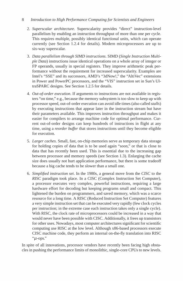
real dependency pseudodependency general version
do i=2,N
A(i)=s*A(i-1)
enddo
do i=1,N-1
A(i)=s*A(i+1)
enddo
start=max(1,1-offset)
end=min(N,N-offset)
do i=start,end
A(i)=s*A(i+offset)
enddo
As the loop is traversed from small to large indices, it makes a huge differencewhether the offset is negative or positive. In the latter case we speak of a pseudo-
dependency, because A(i+1) is always available when the pipeline needs it forcomputing A(i), i.e., there is no stall. In case of a real dependency, however, thepipelined computation of A(i) must stall until the result A(i-1) is completelyfinished. This causes a massive drop in performance as can be seen on the left ofFigure 1.7. The graph shows the performance of above scaling loop in MFlops/secversus loop length. The drop is clearly visible only in cache because of the smalllatencies and large bandwidths of on-chip caches. If the loop length is so large thatall data has to be fetched from memory, the impact of pipeline stalls is much lesssignificant, because those extra cycles easily overlap with the time the core has towait for off-chip data.
Although one might expect that it should make no difference whether the offsetis known at compile time, the right graph in Figure 1.7 shows that there is a dramaticperformance penalty for a variable offset. The compiler can obviously not optimallysoftware pipeline or otherwise optimize the loop in this case. This is actually a com-mon phenomenon, not exclusively related to software pipelining; hiding informationfrom the compiler can have a substantial performance impact (in this particular case,the compiler refrains from SIMD vectorization; see Section 1.2.4 and also Prob-lems 1.2 and 2.2).
There are issues with software pipelining linked to the use of caches. See Sec-tion 1.3.3 below for details.
1.2.4 Superscalarity
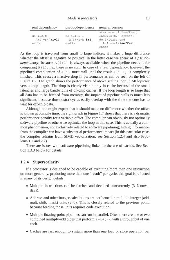
If a processor is designed to be capable of executing more than one instructionor, more generally, producing more than one “result” per cycle, this goal is reflectedin many of its design details:
• Multiple instructions can be fetched and decoded concurrently (3–6 nowa-days).
• Address and other integer calculations are performed in multiple integer (add,mult, shift, mask) units (2–6). This is closely related to the previous point,because feeding those units requires code execution.
• Multiple floating-point pipelines can run in parallel. Often there are one or twocombined multiply-add pipes that perform a=b+c*d with a throughput of oneeach.
• Caches are fast enough to sustain more than one load or store operation per

14 Introduction to High Performance Computing for Scientists and Engineers
32 32 32 32
x x x x4 3 2 1
y y y y4 3 2 1
r r r r4 3 2 1
Figure 1.8: Example for SIMD: Single precision FP addition of two SIMD registers (x,y),each having a length of 128 bits. Four SP flops are executed in a single instruction.
cycle, and the number of available execution units for loads and stores reflectsthat (2–4).
Superscalarity is a special form of parallel execution, and a variant of instruction-
level parallelism (ILP). Out-of-order execution and compiler optimization must worktogether in order to fully exploit superscalarity. However, even on the most advancedarchitectures it is extremely hard for compiler-generated code to achieve a throughputof more than 2–3 instructions per cycle. This is why applications with very highdemands for performance sometimes still resort to the use of assembly language.
1.2.5 SIMD
The SIMD concept became widely known with the first vector supercomputersin the 1970s (see Section 1.6), and was the fundamental design principle for themassively parallel Connection Machines in the 1980s and early 1990s [R36].
Many recent cache-based processors have instruction set extensions for both in-teger and floating-point SIMD operations [V107], which are reminiscent of thosehistorical roots but operate on a much smaller scale. They allow the concurrent ex-ecution of arithmetic operations on a “wide” register that can hold, e.g., two DP orfour SP floating-point words. Figure 1.8 shows an example, where two 128-bit reg-isters hold four single-precision floating-point values each. A single instruction caninitiate four additions at once. Note that SIMD does not specify anything about thepossible concurrency of those operations; the four additions could be truly parallel,if sufficient arithmetic units are available, or just be fed to a single pipeline. Whilethe latter strategy uses SIMD as a device to reduce superscalarity (and thus complex-ity) without sacrificing peak arithmetic performance, the former option boosts peakperformance. In both cases the memory subsystem (or at least the cache) must beable to sustain sufficient bandwidth to keep all units busy. See Section 2.3.3 for theprogramming and optimization implications of SIMD instruction sets.

Modern processors 15
1.3 Memory hierarchies
Data can be stored in a computer system in many different ways. As describedabove, CPUs have a set of registers, which can be accessed without delay. In ad-dition there are one or more small but very fast caches holding copies of recentlyused data items. Main memory is much slower, but also much larger than cache. Fi-nally, data can be stored on disk and copied to main memory as needed. This a is acomplex hierarchy, and it is vital to understand how data transfer works between thedifferent levels in order to identify performance bottlenecks. In the following we willconcentrate on all levels from CPU to main memory (see Figure 1.3).
1.3.1 Cache
Caches are low-capacity, high-speed memories that are commonly integrated onthe CPU die. The need for caches can be easily understood by realizing that datatransfer rates to main memory are painfully slow compared to the CPU’s arithmeticperformance. While peak performance soars at several GFlops/sec per core, memory
bandwidth, i.e., the rate at which data can be transferred from memory to the CPU,is still stuck at a couple of GBytes/sec, which is entirely insufficient to feed all arith-metic units and keep them busy continuously (see Chapter 3 for a more thoroughanalysis). To make matters worse, in order to transfer a single data item (usuallyone or two DP words) from memory, an initial waiting time called latency passesuntil data can actually flow. Thus, latency is often defined as the time it takes totransfer a zero-byte message. Memory latency is usually of the order of several hun-dred CPU cycles and is composed of different contributions from memory chips, thechipset and the processor. Although Moore’s Law still guarantees a constant rate ofimprovement in chip complexity and (hopefully) performance, advances in memoryperformance show up at a much slower rate. The term DRAM gap has been coinedfor the increasing “distance” between CPU and memory in terms of latency andbandwidth [R34, R37].
Caches can alleviate the effects of the DRAM gap in many cases. Usually thereare at least two levels of cache (see Figure 1.3), called L1 and L2, respectively. L1 isnormally split into two parts, one for instructions (“I-cache,” “L1I”) and one for data(“L1D”). Outer cache levels are normally unified, storing data as well as instructions.In general, the “closer” a cache is to the CPU’s registers, i.e., the higher its bandwidthand the lower its latency, the smaller it must be to keep administration overhead low.Whenever the CPU issues a read request (“load”) for transferring a data item to aregister, first-level cache logic checks whether this item already resides in cache. Ifit does, this is called a cache hit and the request can be satisfied immediately, withlow latency. In case of a cache miss, however, data must be fetched from outer cachelevels or, in the worst case, from main memory. If all cache entries are occupied, ahardware-implemented algorithm evicts old items from cache and replaces them withnew data. The sequence of events for a cache miss on a write is more involved and

16 Introduction to High Performance Computing for Scientists and Engineers
Figure 1.9: The perfor-mance gain from access-ing data from cache ver-sus the cache reuse ra-tio, with the speed ad-vantage of cache ver-sus main memory beingparametrized by τ . 0.7 0.75 0.8 0.85 0.9 0.95 1
β
0
5
10
15
20
G(τ
,β)
τ=5
τ=10
τ=50
will be described later. Instruction caches are usually of minor importance since sci-entific codes tend to be largely loop-based; I-cache misses are rare events comparedto D-cache misses.
Caches can only have a positive effect on performance if the data access patternof an application shows some locality of reference. More specifically, data items thathave been loaded into a cache are to be used again “soon enough” to not have beenevicted in the meantime. This is also called temporal locality. Using a simple model,we will now estimate the performance gain that can be expected from a cache thatis a factor of τ faster than memory (this refers to bandwidth as well as latency; amore refined model is possible but does not lead to additional insight). Let β be thecache reuse ratio, i.e., the fraction of loads or stores that can be satisfied from cachebecause there was a recent load or store to the same address. Access time to mainmemory (again this includes latency and bandwidth) is denoted by Tm. In cache,access time is reduced to Tc = Tm/τ . For some finite β , the average access time willthus be Tav = βTc +(1−β )Tm, and we calculate an access performance gain of
G(τ,β ) =Tm
Tav=
τTc
βTc +(1−β )τTc=
τ
β + τ(1−β ). (1.4)
As Figure 1.9 shows, a cache can only lead to a significant performance advantage ifthe reuse ratio is relatively close to one.
Unfortunately, supporting temporal locality is not sufficient. Many applicationsshow streaming patterns where large amounts of data are loaded into the CPU, mod-ified, and written back without the potential of reuse “in time.” For a cache that onlysupports temporal locality, the reuse ratio β (see above) is zero for streaming. Eachnew load is expensive as an item has to be evicted from cache and replaced by thenew one, incurring huge latency. In order to reduce the latency penalty for streaming,caches feature a peculiar organization into cache lines. All data transfers betweencaches and main memory happen on the cache line level (there may be exceptionsfrom that rule; see the comments on nontemporal stores on page 18 for details). The

Modern processors 17
advantage of cache lines is that the latency penalty of a cache miss occurs only onthe first miss on an item belonging to a line. The line is fetched from memory as awhole; neighboring items can then be loaded from cache with much lower latency,increasing the cache hit ratio γ , not to be confused with the reuse ratio β . So if theapplication shows some spatial locality, i.e., if the probability of successive accessesto neighboring items is high, the latency problem can be significantly reduced. Thedownside of cache lines is that erratic data access patterns are not supported. On thecontrary, not only does each load incur a miss and subsequent latency penalty, it alsoleads to the transfer of a whole cache line, polluting the memory bus with data thatwill probably never be used. The effective bandwidth available to the application willthus be very low. On the whole, however, the advantages of using cache lines pre-vail, and very few processor manufacturers have provided means of bypassing themechanism.
Assuming a streaming application working on DP floating point data on a CPUwith a cache line length of Lc = 16 words, spatial locality fixes the hit ratio at γ =(16 − 1)/16 = 0.94, a seemingly large value. Still it is clear that performance isgoverned by main memory bandwidth and latency — the code is memory-bound. Inorder for an application to be truly cache-bound, i.e., decouple from main memory sothat performance is not governed by memory bandwidth or latency any more, γ mustbe large enough so the time it takes to process in-cache data becomes larger than thetime for reloading it. If and when this happens depends of course on the details ofthe operations performed.
By now we can qualitatively interpret the performance data for cache-based ar-chitectures on the vector triad in Figure 1.4. At very small loop lengths, the processorpipeline is too long to be efficient. With growing N this effect becomes negligible,and as long as all four arrays fit into the innermost cache, performance saturates ata high value that is set by the L1 cache bandwidth and the ability of the CPU to is-sue load and store instructions. Increasing N a little more gives rise to a sharp dropin performance because the innermost cache is not large enough to hold all data.Second-level cache has usually larger latency but similar bandwidth to L1 so thatthe penalty is larger than expected. However, streaming data from L2 has the disad-vantage that L1 now has to provide data for registers as well as continuously reloadand evict cache lines from/to L2, which puts a strain on the L1 cache’s bandwidthlimits. Since the ability of caches to deliver data to higher and lower hierarchy levelsconcurrently is highly architecture-dependent, performance is usually hard to predicton all but the innermost cache level and main memory. For each cache level anotherperformance drop is observed with rising N, until finally even the large outer cache istoo small and all data has to be streamed from main memory. The size of the differentcaches is directly related to the locations of the bandwidth breakdowns. Section 3.1will describe how to predict performance for simple loops from basic parameters likecache or memory bandwidths and the data demands of the application.
Storing data is a little more involved than reading. In presence of caches, if datato be written out already resides in cache, a write hit occurs. There are several pos-sibilities for handling this case, but usually outermost caches work with a write-back
strategy: The cache line is modified in cache and written to memory as a whole when

18 Introduction to High Performance Computing for Scientists and Engineers
evicted. On a write miss, however, cache-memory consistency dictates that the cacheline in question must first be transferred from memory to cache before an entry canbe modified. This is called write allocate, and leads to the situation that a data writestream from CPU to memory uses the bus twice: once for all the cache line alloca-tions and once for evicting modified lines (the data transfer requirement for the triadbenchmark code is increased by 25% due to write allocates). Consequently, stream-ing applications do not usually profit from write-back caches and there is often a wishfor avoiding write-allocate transactions. Some architectures provide this option, andthere are generally two different strategies:
• Nontemporal stores. These are special store instructions that bypass all cachelevels and write directly to memory. Cache does not get “polluted” by storestreams that do not exhibit temporal locality anyway. In order to prevent ex-cessive latencies, there is usually a small write combine buffer, which bundlesa number of successive nontemporal stores [V104].
• Cache line zero. Special instructions “zero out” a cache line and mark it asmodified without a prior read. The data is written to memory when evicted.In comparison to nontemporal stores, this technique uses up cache space forthe store stream. On the other hand it does not slow down store operations incache-bound situations. Cache line zero must be used with extreme care: Allelements of a cache line are evicted to memory, even if only a part of themwere actually modified.
Both can be applied by the compiler and hinted at by the programmer by meansof directives. In very simple cases compilers are able to apply those instructionsautomatically in their optimization stages, but one must take care to not slow downa cache-bound code by using nontemporal stores, rendering it effectively memory-bound.
Note that the need for write allocates arises because caches and memory gener-ally communicate in units of cache lines; it is a common misconception that writeallocates are only required to maintain consistency between caches of multiple pro-cessor cores.
1.3.2 Cache mapping
So far we have implicitly assumed that there is no restriction on which cache linecan be associated with which memory locations. A cache design that follows thisrule is called fully associative. Unfortunately it is quite hard to build large, fast, andfully associative caches because of large bookkeeping overhead: For each cache linethe cache logic must store its location in the CPU’s address space, and each mem-ory access must be checked against the list of all those addresses. Furthermore, thedecision which cache line to replace next if the cache is full is made by some algo-rithm implemented in hardware. Often there is a least recently used (LRU) strategythat makes sure only the “oldest” items are evicted, but alternatives like NRU (not
recently used) or random replacement are possible.

Modern processors 19
����
����
����
����
��
��
��
��
��
��
��
��
��
��
��
��
����
����
����
����
����
����
����
����
��
��
��
��
Ca
ch
e
Memory
Figure 1.10: In a direct-mapped cache, memory locations which lie a multiple of the cachesize apart are mapped to the same cache line (shaded boxes).
The most straightforward simplification of this expensive scheme consists in adirect-mapped cache, which maps the full cache size repeatedly into memory (seeFigure 1.10). Memory locations that lie a multiple of the cache size apart are alwaysmapped to the same cache line, and the cache line that corresponds to some addresscan be obtained very quickly by masking out the most significant bits. Moreover, analgorithm to select which cache line to evict is pointless. No hardware and no clockcycles need to be spent for it.
The downside of a direct-mapped cache is that it is disposed toward cache thrash-
ing, which means that cache lines are loaded into and evicted from the cache in rapidsuccession. This happens when an application uses many memory locations that getmapped to the same cache line. A simple example would be a “strided” vector triadcode for DP data, which is obtained by modifying the inner loop as follows:
1 do i=1,N,CACHE_SIZE_IN_BYTES/8
2 A(i) = B(i) + C(i) * D(i)
3 enddo
By using the cache size in units of DP words as a stride, successive loop iterationshit the same cache line so that every memory access generates a cache miss, eventhough a whole line is loaded every time. In principle there is plenty of room left inthe cache, so this kind of situation is called a conflict miss. If the stride were equal tothe line length there would still be some (albeit small) N for which the cache reuse is100%. Here, the reuse fraction is exactly zero no matter how small N may be.
To keep administrative overhead low and still reduce the danger of conflict missesand cache thrashing, a set-associative cache is divided into m direct-mapped caches

20 Introduction to High Performance Computing for Scientists and Engineers
����
����
����
����
����
��
����
��
��
��
����
��
��
��
����
��
��
����
��������
����
����
����
��������
����
����
��
����
��
��
Cache
Memory
Way 1Way 2
Figure 1.11: In an m-way set-associative cache, memory locations which are located a mul-tiple of 1
m th of the cache size apart can be mapped to either of m cache lines (here shown form = 2).
equal in size, so-called ways. The number of ways m is the number of different cachelines a memory address can be mapped to (see Figure 1.11 for an example of atwo-way set-associative cache). On each memory access, the hardware merely has todetermine which way the data resides in or, in the case of a miss, to which of the m
possible cache lines it should be loaded.For each cache level the tradeoff between low latency and prevention of thrashing
must be considered by processor designers. Innermost (L1) caches tend to be lessset-associative than outer cache levels. Nowadays, set-associativity varies betweentwo- and 48-way. Still, the effective cache size, i.e., the part of the cache that isactually useful for exploiting spatial and temporal locality in an application codecould be quite small, depending on the number of data streams, their strides andmutual offsets. See Chapter 3 for examples.
1.3.3 Prefetch
Although exploiting spatial locality by the introduction of cache lines improvescache efficiency a lot, there is still the problem of latency on the first miss. Figure 1.12visualizes the situation for a simple vector norm kernel:
1 do i=1,N
2 S = S + A(i)*A(i)
3 enddo
There is only one load stream in this code. Assuming a cache line length of fourelements, three loads can be satisfied from cache before another miss occurs. Thelong latency leads to long phases of inactivity on the memory bus.

Modern processors 21
1
2
3
4
5
6
7
Ite
rati
on
#
time
LD cache miss: latency use data
use data
use data
use data
cache miss: latencyLD use data
use data
use dataLD
LD
LD
LD
LD
Figure 1.12: Timing diagram on the influence of cache misses and subsequent latency penal-ties for a vector norm loop. The penalty occurs on each new miss.
Making the lines very long will help, but will also slow down applications witherratic access patterns even more. As a compromise one has arrived at typical cacheline lengths between 64 and 128 bytes (8–16 DP words). This is by far not big enoughto get around latency, and streaming applications would suffer not only from insuffi-cient bandwidth but also from low memory bus utilization. Assuming a typical com-modity system with a memory latency of 50 ns and a bandwidth of 10 GBytes/sec,a single 128-byte cache line transfer takes 13 ns, so 80% of the potential bus band-width is unused. Latency has thus an even more severe impact on performance thanbandwidth.
The latency problem can be solved in many cases, however, by prefetching. Pre-fetching supplies the cache with data ahead of the actual requirements of an applica-tion. The compiler can do this by interleaving special instructions with the softwarepipelined instruction stream that “touch” cache lines early enough to give the hard-ware time to load them into cache asynchronously (see Figure 1.13). This assumesthere is the potential of asynchronous memory operations, a prerequisite that is tosome extent true for current architectures. As an alternative, some processors featurea hardware prefetcher that can detect regular access patterns and tries to read aheadapplication data, keeping up the continuous data stream and hence serving the samepurpose as prefetch instructions. Whichever strategy is used, it must be emphasizedthat prefetching requires resources that are limited by design. The memory subsys-tem must be able to sustain a certain number of outstanding prefetch operations,i.e., pending prefetch requests, or else the memory pipeline will stall and latencycannot be hidden completely. We can estimate the number of outstanding prefetchesrequired for hiding the latency completely: If Tℓ is the latency and B is the bandwidth,the transfer of a whole line of length Lc (in bytes) takes a time of
T = Tℓ +Lc
B. (1.5)
One prefetch operation must be initiated per cache line transfer, and the number ofcache lines that can be transferred during time T is the number of prefetches P that

22 Introduction to High Performance Computing for Scientists and Engineers
1
2
3
4
5
6
7
Ite
rati
on
#
8
9
time
use data
use data
use data
use data
use data
use data
use data
use data
use dataLD
LD
LD
PF cache miss: latency
PF cache miss: latency
LD
LD
LD
LD
LD
LD
cache miss: latencyPF
Figure 1.13: Computation and data transfer can be overlapped much better with prefetching.In this example, two outstanding prefetches are required to hide latency completely.
the processor must be able to sustain (see Figure 1.13):
P =T
Lc/B= 1+
Tℓ
Lc/B. (1.6)
As an example, for a cache line length of 128 bytes (16 DP words), B =10 GBytes/sec and Tℓ = 50 ns we get P≈ 5 outstanding prefetches. If this requirementcannot be met, latency will not be hidden completely and the full memory bandwidthwill not be utilized. On the other hand, an application that executes so many floating-point operations on the cache line data that they cannot be hidden behind the transferwill not be limited by bandwidth and put less strain on the memory subsystem (seeSection 3.1 for appropriate performance models). In such a case, fewer outstandingprefetches will suffice.
Applications with heavy demands on bandwidth can overstrain the prefetchmechanism. A second processor core using a shared path to memory can sometimesprovide for the missing prefetches, yielding a slight bandwidth boost (see Section 1.4for more information on multicore design). In general, if streaming-style main mem-ory access is unavoidable, a good programming guideline is to try to establish longcontinuous data streams.
Finally, a note of caution is in order. Figures 1.12 and 1.13 stress the role ofprefetching for hiding latency, but the effects of bandwidth limitations are ignored.It should be clear that prefetching cannot enhance available memory bandwidth, al-though the transfer time for a single cache line is dominated by latency.

Modern processors 23
2 4 8 16m
-0.6
-0.5
-0.4
-0.3
-0.2
-0.1
0
ε f Figure 1.14: Requiredrelative frequency re-duction to stay within agiven power envelopeon a given process tech-nology, versus numberof cores on a multicorechip (or package).
1.4 Multicore processors
In recent years it has become increasingly clear that, although Moore’s Law isstill valid and will probably be at least for the next decade, standard microproces-sors are starting to hit the “heat barrier”: Switching and leakage power of several-hundred-million-transistor chips are so large that cooling becomes a primary engi-neering effort and a commercial concern. On the other hand, the necessity of anever-increasing clock frequency is driven by the insight that architectural advancesand growing cache sizes alone will not be sufficient to keep up the one-to-one cor-respondence of Moore’s Law with application performance. Processor vendors arelooking for a way out of this power-performance dilemma in the form of multicore
designs.The technical motivation behind multicore is based on the observation that, for
a given semiconductor process technology, power dissipation of modern CPUs isproportional to the third power of clock frequency fc (actually it is linear in fc andquadratic in supply voltage Vcc, but a decrease in fc allows for a proportional decreasein Vcc). Lowering fc and thus Vcc can therefore dramatically reduce power dissipation.Assuming that a single core with clock frequency fc has a performance of p and apower dissipation of W , some relative change in performance εp = ∆p/p will emergefor a relative clock change of ε f = ∆ fc/ fc. All other things being equal, |ε f | is anupper limit for |εp|, which in turn will depend on the applications considered. Powerdissipation is
W +∆W = (1+ ε f )3W . (1.7)
Reducing clock frequency opens the possibility to place more than one CPU coreon the same die (or, more generally, into the same package) while keeping the samepower envelope as before. For m “slow” cores this condition is expressed as
(1+ ε f )3m = 1 =⇒ ε f = m−1/3 −1 . (1.8)

24 Introduction to High Performance Computing for Scientists and Engineers
PL1D
L2
L3
PL1D
L2
L3
Figure 1.15: Dual-core processor chip withseparate L1, L2, and L3 caches (Intel “Mon-tecito”). Each core constitutes its own cachegroup on all levels.
L1D L1D
L2
L1D
L2
L1D
PPPP
Figure 1.16: Quad-core processor chip, con-sisting of two dual-cores. Each dual-corehas shared L2 and separate L1 caches (Intel“Harpertown”). There are two dual-core L2groups.
Each one of those cores has the same transistor count as the single “fast” core, butwe know that Moore’s Law gives us transistors for free. Figure 1.14 shows the re-quired relative frequency reduction with respect to the number of cores. The overallperformance of the multicore chip,
pm = (1+ εp)pm , (1.9)
should at least match the single-core performance so that
εp >1m−1 (1.10)
is a limit on the performance penalty for a relative clock frequency reduction of ε f
that should be observed for multicore to stay useful.Of course it is not trivial to grow the CPU die by a factor of m with a given man-
ufacturing technology. Hence, the most simple way to multicore is to place separateCPU dies in a common package. At some point advances in manufacturing tech-nology, i.e., smaller structure lengths, will then enable the integration of more coreson a die. Additionally, some compromises regarding the single-core performance ofa multicore chip with respect to the previous generation will be made so that thenumber of transistors per core will go down as will the clock frequency. Some manu-facturers have even adopted a more radical approach by designing new, much simplercores, albeit at the cost of possibly introducing new programming paradigms.
Finally, the over-optimistic assumption (1.9) that m cores show m times the per-formance of a single core will only be valid in the rarest of cases. Nevertheless,multicore has by now been adopted by all major processor manufacturers. In order toavoid any misinterpretation we will always use the terms “core,” “CPU,” and “pro-cessor” synonymously. A “socket” is the physical package in which multiple cores(sometimes on multiple chips) are enclosed; it is usually equipped with leads or pinsso it can be used as a replaceable component. Typical desktop PCs have a singlesocket, while standard servers use two to four, all sharing the same memory. SeeSection 4.2 for an overview of shared-memory parallel computer architectures.

Modern processors 25
P P P P P PL1DL1DL1D
L2
L1D
L2
L1DL1D
L2
L3
Figure 1.17: Hexa-core processor chip withseparate L1 caches, shared L2 caches forpairs of cores and a shared L3 cache for allcores (Intel “Dunnington”). L2 groups aredual-cores, and the L3 group is the wholechip.
HT/QPI
L1D
L2
PL1D
L2
PL1D
L2
PL1D
L2
P
L3
Memory Interface
Figure 1.18: Quad-core processor chip withseparate L1 and L2 and a shared L3 cache(AMD “Shanghai” and Intel “Nehalem”).There are four single-core L2 groups, and theL3 group is the whole chip. A built-in mem-ory interface allows to attach memory andother sockets directly without a chipset.
There are significant differences in how the cores on a chip or socket may bearranged:
• The cores on one die can either have separate caches (Figure 1.15) or sharecertain levels (Figures 1.16–1.18). For later reference, we will call a group ofcores that share a certain cache level a cache group. For instance, the hexa-corechip in Figure 1.17 comprises six L1 groups (one core each), three dual-coreL2 groups, and one L3 group which encompasses the whole socket.
Sharing a cache enables communication between cores without reverting tomain memory, reducing latency and improving bandwidth by about an orderof magnitude. An adverse effect of sharing could be possible cache bandwidthbottlenecks. The performance impact of shared and separate caches on appli-cations is highly code- and system-dependent. Later sections will provide moreinformation on this issue.
• Most recent multicore designs feature an integrated memory controller towhich memory modules can be attached directly without separate logic(“chipset”). This reduces main memory latency and allows the addition of fastintersocket networks like HyperTransport or QuickPath (Figure 1.18).
• There may exist fast data paths between caches to enable, e.g., efficient cachecoherence communication (see Section 4.2.1 for details on cache coherence).
The first important conclusion one must draw from the multicore transition is theabsolute necessity to put those resources to efficient use by parallel programming,instead of relying on single-core performance. As the latter will at best stagnate overthe years, getting more speed for free through Moore’s law just by waiting for thenew CPU generation does not work any more. Chapter 5 outlines the principles andlimitations of parallel programming. More details on dual- and multicore designs willbe revealed in Section 4.2, which covers shared-memory architectures. Chapters 6

26 Introduction to High Performance Computing for Scientists and Engineers
and 9 introduce the dominating parallel programming paradigms in use for technicaland scientific computing today.
Another challenge posed by multicore is the gradual reduction in main memorybandwidth and cache size available per core. Although vendors try to compensatethese effects with larger caches, the performance of some algorithms is always boundby main memory bandwidth, and multiple cores sharing a common memory bussuffer from contention. Programming techniques for traffic reduction and efficientbandwidth utilization are hence becoming paramount for enabling the benefits ofMoore’s Law for those codes as well. Chapter 3 covers some techniques that areuseful in this context.
Finally, the complex structure of shared and nonshared caches on current multi-core chips (see Figures 1.17 and 1.18) makes communication characteristics betweendifferent cores highly nonisotropic: If there is a shared cache, two cores can exchangecertain amounts of information much faster; e.g., they can synchronize via a variablein cache instead of having to exchange data over the memory bus (see Sections 7.2and 10.5 for practical consequences). At the time of writing, there are very few truly“multicore-aware” programming techniques that explicitly exploit this most impor-tant feature to improve performance of parallel code [O52, O53].
Therefore, depending on the communication characteristics and bandwidth de-mands of running applications, it can be extremely important where exactly multiplethreads or processes are running in a multicore (and possibly multisocket) environ-ment. Appendix A provides details on how affinity between hardware entities (cores,sockets) and “programs” (processes, threads) can be established. The impact of affin-ity on the performance characteristics of parallel programs will be encountered fre-quently in this book, e.g., in Section 6.2, Chapters 7 and 8, and Section 10.5.
1.5 Multithreaded processors
All modern processors are heavily pipelined, which opens the possibility for highperformance if the pipelines can actually be used. As described in previous sections,several factors can inhibit the efficient use of pipelines: Dependencies, memory la-tencies, insufficient loop length, unfortunate instruction mix, branch misprediction(see Section 2.3.2), etc. These lead to frequent pipeline bubbles, and a large part ofthe execution resources remains idle (see Figure 1.19). Unfortunately this situationis the rule rather than the exception. The tendency to design longer pipelines in orderto raise clock speeds and the general increase in complexity adds to the problem.As a consequence, processors become hotter (dissipate more power) without a pro-portional increase in average application performance, an effect that is only partiallycompensated by the multicore transition.
For this reason, threading capabilities are built into many current processor de-signs. Hyper-Threading [V108, V109] or SMT (Simultaneous Multithreading) arefrequent names for this feature. Common to all implementations is that the architec-
tural state of a CPU core is present multiple times. The architectural state comprises
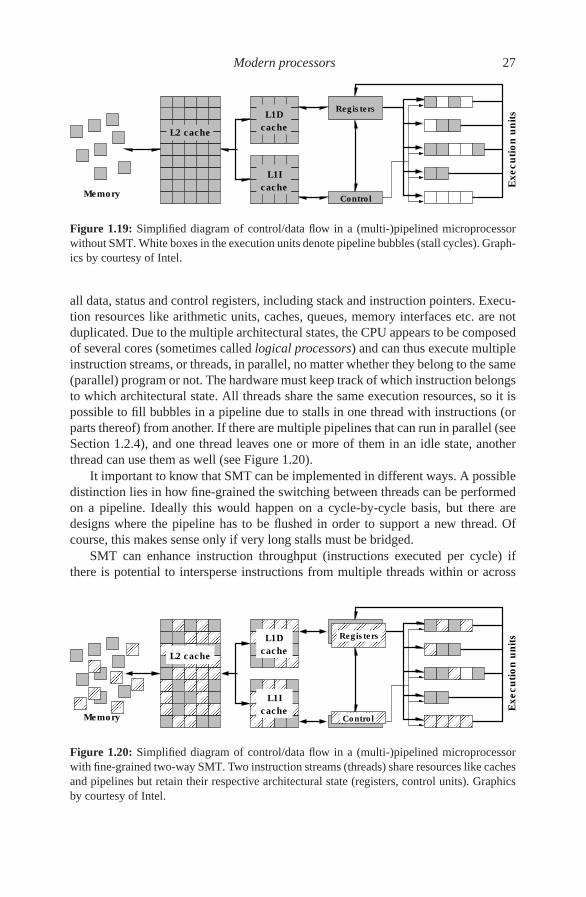
Modern processors 27
L1D
cache
L1I
cacheMemory
L2 cache
Control
Registers
Ex
ec
uti
on
un
its
Figure 1.19: Simplified diagram of control/data flow in a (multi-)pipelined microprocessorwithout SMT. White boxes in the execution units denote pipeline bubbles (stall cycles). Graph-ics by courtesy of Intel.
all data, status and control registers, including stack and instruction pointers. Execu-tion resources like arithmetic units, caches, queues, memory interfaces etc. are notduplicated. Due to the multiple architectural states, the CPU appears to be composedof several cores (sometimes called logical processors) and can thus execute multipleinstruction streams, or threads, in parallel, no matter whether they belong to the same(parallel) program or not. The hardware must keep track of which instruction belongsto which architectural state. All threads share the same execution resources, so it ispossible to fill bubbles in a pipeline due to stalls in one thread with instructions (orparts thereof) from another. If there are multiple pipelines that can run in parallel (seeSection 1.2.4), and one thread leaves one or more of them in an idle state, anotherthread can use them as well (see Figure 1.20).
It important to know that SMT can be implemented in different ways. A possibledistinction lies in how fine-grained the switching between threads can be performedon a pipeline. Ideally this would happen on a cycle-by-cycle basis, but there aredesigns where the pipeline has to be flushed in order to support a new thread. Ofcourse, this makes sense only if very long stalls must be bridged.
SMT can enhance instruction throughput (instructions executed per cycle) ifthere is potential to intersperse instructions from multiple threads within or across
������������
������������
���������
���������
���������������
���������������
������
������
������������
��������
���������
���������
������������
������
������
������
������
������
������
���������
���������
���������
���������
���������
���������
��������
������������
��������
��������������������
������������
������������
��������
��������������������
���������
���������
������������
���������
���������
������
������ ��
������
��������
��������
��������
������������
������������
������
������
���������
���������
������������
������
������ ��
������
������������
���������
���������
������
��������������
��������
������
������
��������
������
������
���������
���������������������
��������������������
������
������
������������
��������
��������
������������������������������������
������������������������������������
������������������������������������
���������������������������
���������������������������
L1D
cache
L1I
cacheMemory
L2 cache
Registers
Control
Ex
ec
uti
on
un
its
Figure 1.20: Simplified diagram of control/data flow in a (multi-)pipelined microprocessorwith fine-grained two-way SMT. Two instruction streams (threads) share resources like cachesand pipelines but retain their respective architectural state (registers, control units). Graphicsby courtesy of Intel.
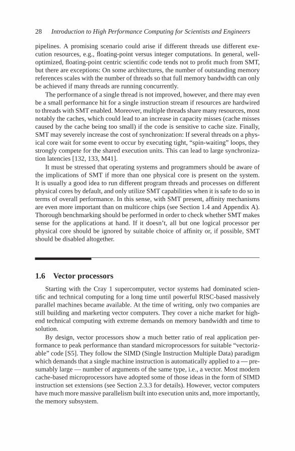
28 Introduction to High Performance Computing for Scientists and Engineers
pipelines. A promising scenario could arise if different threads use different exe-cution resources, e.g., floating-point versus integer computations. In general, well-optimized, floating-point centric scientific code tends not to profit much from SMT,but there are exceptions: On some architectures, the number of outstanding memoryreferences scales with the number of threads so that full memory bandwidth can onlybe achieved if many threads are running concurrently.
The performance of a single thread is not improved, however, and there may evenbe a small performance hit for a single instruction stream if resources are hardwiredto threads with SMT enabled. Moreover, multiple threads share many resources, mostnotably the caches, which could lead to an increase in capacity misses (cache missescaused by the cache being too small) if the code is sensitive to cache size. Finally,SMT may severely increase the cost of synchronization: If several threads on a phys-ical core wait for some event to occur by executing tight, “spin-waiting” loops, theystrongly compete for the shared execution units. This can lead to large synchroniza-tion latencies [132, 133, M41].
It must be stressed that operating systems and programmers should be aware ofthe implications of SMT if more than one physical core is present on the system.It is usually a good idea to run different program threads and processes on differentphysical cores by default, and only utilize SMT capabilities when it is safe to do so interms of overall performance. In this sense, with SMT present, affinity mechanismsare even more important than on multicore chips (see Section 1.4 and Appendix A).Thorough benchmarking should be performed in order to check whether SMT makessense for the applications at hand. If it doesn’t, all but one logical processor perphysical core should be ignored by suitable choice of affinity or, if possible, SMTshould be disabled altogether.
1.6 Vector processors
Starting with the Cray 1 supercomputer, vector systems had dominated scien-tific and technical computing for a long time until powerful RISC-based massivelyparallel machines became available. At the time of writing, only two companies arestill building and marketing vector computers. They cover a niche market for high-end technical computing with extreme demands on memory bandwidth and time tosolution.
By design, vector processors show a much better ratio of real application per-formance to peak performance than standard microprocessors for suitable “vectoriz-able” code [S5]. They follow the SIMD (Single Instruction Multiple Data) paradigmwhich demands that a single machine instruction is automatically applied to a — pre-sumably large — number of arguments of the same type, i.e., a vector. Most moderncache-based microprocessors have adopted some of those ideas in the form of SIMDinstruction set extensions (see Section 2.3.3 for details). However, vector computershave much more massive parallelism built into execution units and, more importantly,the memory subsystem.

Modern processors 29
Scalar unit
Ve
cto
r re
gis
ters
Ma
in m
em
ory
Scalar
exec.
units
Ca
ch
e
Mask reg.
Scalarreg.
ADD/
SHIFT
MULT
DIV/
SQRT
LOGIC
LD/ST
Figure 1.21: Block diagram of a prototypical vector processor with 4-track pipelines.
1.6.1 Design principles
Current vector processors are, quite similarly to RISC designs, register-to-registermachines: Machine instructions operate on vector registers which can hold a numberof arguments, usually between 64 and 256 (double precision). The width of a vectorregister is called the vector length Lv. There is a pipeline for each arithmetic opera-tion like addition, multiplication, divide, etc., and each pipeline can deliver a certainnumber of results per cycle. For MULT and ADD pipes, this number varies betweentwo and 16 and one speaks of a multitrack pipeline (see Figure 1.21 for a block di-agram of a prototypical vector processor with 4-track pipes). Other operations likesquare root and divide are significantly more complex, hence the pipeline throughputis much lower for them. A vector processor with single-track pipes can achieve asimilar peak performance per clock cycle as a superscalar cache-based microproces-sor. In order to supply data to the vector registers, there is one or more load, store orcombined load/store pipes connecting directly to main memory. Classic vector CPUshave no concept of cache hierarchies, although recent designs like the NEC SX-9have introduced small on-chip memories.
For getting reasonable performance out of a vector CPU, SIMD-type instructionsmust be employed. As a simple example we consider the addition, of two arrays:A(1:N)=B(1:N)+C(1:N). On a cache-based microprocessor this would resultin a (possibly software-pipelined) loop over the elements of A, B, and C. For eachindex, two loads, one addition and one store operation would have to be executed,

30 Introduction to High Performance Computing for Scientists and Engineers
together with the required integer and branch logic to perform the loop. A vectorCPU can issue a single instruction for a whole array if it is shorter than the vectorlength:
1 vload V1(1:N) = B(1:N)
2 vload V2(1:N) = C(1:N)
3 vadd V3(1:N) = V1(1:N) + V2(1:N)
4 vstore A(1:N) = V3(1:N)
Here, V1, V2, and V3 denote vector registers. The distribution of vector indicesacross the pipeline tracks is automatic. If the array length is larger than the vectorlength, the loop must be stripmined, i.e., the original arrays are traversed in chunksof the vector length:
1 do S = 1,N,Lv2 E = min(N,S+Lv-1)
3 L = E-S+1
4 vload V1(1:L) = B(S:E)
5 vload V2(1:L) = C(S:E)
6 vadd V3(1:L) = V1(1:L) + V2(1:L)
7 vstore A(S:E) = V3(1:L)
8 enddo
This is done automatically by the compiler.
An operation like vector addition does not have to wait until its argument vec-tor registers are completely filled but can commence after some initial argumentsare available. This feature is called chaining and forms an essential requirement fordifferent pipes (like MULT and ADD) to operate concurrently.
Obviously the vector architecture greatly reduces the required instruction issuerate, which had however only been an advantage in the pre-RISC era where multi-issue superscalar processors with fast instruction caches were unavailable. More im-portantly, the speed of the load/store pipes is matched to the CPU’s core frequency,so feeding the arithmetic pipes with data is much less of a problem. This can onlybe achieved with a massively banked main memory layout because current mem-ory chips require some cycles of recovery time, called the bank busy time, after anyaccess. In order to bridge this gap, current vector computers provide thousands ofmemory banks, making this architecture prohibitively expensive for general-purposecomputing. In summary, a vector processor draws its performance by a combinationof massive pipeline parallelism with high-bandwidth memory access.
Writing a program so that the compiler can generate effective SIMD vector in-structions is called vectorization. Sometimes this requires reformulation of code orinserting source code directives in order to help the compiler identify SIMD paral-lelism. A separate scalar unit is present on every vector processor to execute codewhich cannot use the vector units for some reason (see also the following sections)and to perform administrative tasks. Today, scalar units in vector processors are muchinferior to standard RISC or x86-based designs, so vectorization is absolutely vitalfor getting good performance. If a code cannot be vectorized it does not make senseto use a vector computer at all.

Modern processors 31
A(:) = B(:) + C(:) * D(:)
LOAD BLOAD C LOAD D
ADD
MULT
ADDADD
MULT MULT MULT
ADD
STORE A
time Figure 1.22: Pipelineutilization timeline forexecution of the vectortriad (see Listing 1.1)on the vector processorshown in Figure 1.21.Light gray boxes denoteunused arithmetic units.
1.6.2 Maximum performance estimates
The peak performance of a vector processor is given by the number of tracks forthe ADD and MULT pipelines and its clock frequency. For example, a vector CPUrunning at 2 GHz and featuring four-track pipes has a peak performance of
2 (ADD+MULT)×4 (tracks)×2 (GHz)=16 GFlops/sec .
Square root, divide and other operations are not considered here as they do not con-tribute significantly because of their strongly inferior throughput. As for memorybandwidth, a single four-track LD/ST pipeline (see Figure 1.21) can deliver
4 (tracks)×2 (GHz)×8 (bytes)=64 GBytes/sec
for reading or writing. (These happen to be the specifications of an NEC SX-8 pro-cessor.) In contrast to standard cache-based microprocessors, the memory interfaceof vector CPUs often runs at the same frequency as the core, delivering more band-width in relation to peak performance. Note that above calculations assume that thevector units can actually be used — if a code is nonvectorizable, neither peak perfor-mance nor peak memory bandwidth can be achieved, and the (severe) limitations ofthe scalar unit(s) apply.
Often the performance of a given loop kernel with simple memory access patternscan be accurately predicted. Chapter 3 will give a thorough introduction to balanceanalysis, i.e., performance prediction based on architectural properties and loop codecharacteristics. For vector processors, the situation is frequently simple due to theabsence of complications like caches. As an example we choose the vector triad (seeListing 1.1), which performs three loads, one store and two flops (MULT+ADD).As there is only a single LD/ST pipe, loads and stores and even loads to differentarrays cannot overlap each other, but they can overlap arithmetic and be chained toarithmetic pipes. In Figure 1.22 a rhomboid stands for an operation on a vector regis-ter, symbolizing the pipelined execution (much similar to the timeline in Figure 1.5).First a vector register must be loaded with data from array C. As the LD/ST pipestarts filling a vector register with data from array D, the MULT pipe can start per-forming arithmetic on C and D. As soon as data from B is available, the ADD pipe cancompute the final result, which is then stored to memory by the LD/ST pipe again.
The performance of the whole process is obviously limited by the LD/STpipeline; given suitable code, the hardware would be capable of executing four times

32 Introduction to High Performance Computing for Scientists and Engineers
Figure 1.23: On a vec-tor processor, a loop withan if/else branch can bevectorized using a maskregister.
y(1)*y(1)
y(2)*y(2)
y(3)*y(3)
y(4)*y(4)
y(5)*y(5)
y(6)*y(6)
y(7)*y(7)
y(8)*y(8)
FALSE
FALSE
FALSE
FALSE
TRUE
TRUE
TRUE
TRUE
s*y(2)
s*y(3)
s*y(4)
s*y(5)
s*y(6)
s*y(7)
s*y(8)
s*y(1) y(1)*y(1)
y(3)*y(3)
y(4)*y(4)
y(6)*y(6)
s*y(7)
s*y(8)
s*y(2)
s*y(5)
Vector reg. Vector reg. Mask reg. Vector reg.
as many MULTs and ADDs in the same time (light gray rhomboids), so the triadcode runs with 25% of peak performance. On the vector machine described abovethis amounts to 4 GFlops/sec, which is completely in line with large-N data for theSX-8 in Figure 1.4. Note that this limit is only reached for relatively large N, owingto the large memory latencies on a vector system. Apart from nonvectorizable code,short loops are the second important stumbling block which can negatively impactperformance on these architectures.
1.6.3 Programming for vector architectures
A necessary prerequisite for vectorization is the lack of true data dependenciesacross the iterations of a loop. The same restrictions as for software pipelining ap-ply (see Section 1.2.3), i.e., forward references are allowed but backward referencesinhibit vectorization. To be more precise, the offset for the true dependency mustbe larger than some threshold (at least the vector length, sometimes larger) so thatresults from previous vector operations are available.
Branches in inner loop kernels are also a problem with vectorization becausethey contradict the “single instruction” paradigm. However, there are several ways tosupport branches in vectorized loops:
• Mask registers (essentially boolean registers with vector length) are providedthat allow selective execution of loop iterations. As an example we considerthe following loop:
1 do i = 1,N
2 if(y(i) .le. 0.d0) then
3 x(i) = s * y(i)
4 else
5 x(i) = y(i) * y(i)
6 endif
7 enddo
A vector of boolean values is first generated from the branch conditional using
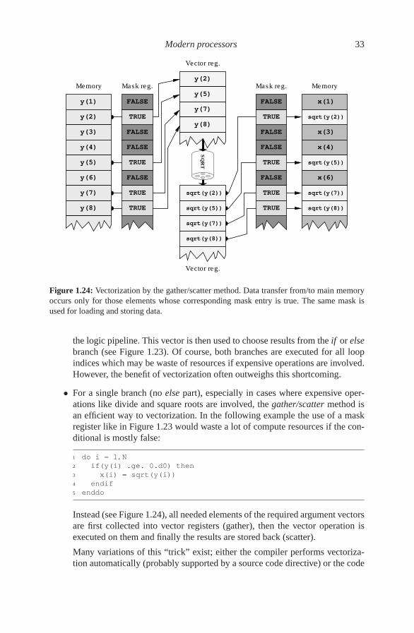
Modern processors 33
y(1)
y(2)
y(3)
y(4)
y(5)
y(6)
y(7)
y(8)
sqrt(y(2))
sqrt(y(5))
sqrt(y(7))
sqrt(y(8))
y(2)
y(5)
y(7)
y(8)
x(1)
x(3)
x(4)
x(6)
sqrt(y(2))
sqrt(y(5))
sqrt(y(7))
sqrt(y(8))
Memory
FALSE
FALSE
FALSE
FALSE
TRUE
TRUE
TRUE
TRUE
Mask reg. Memory
FALSE
FALSE
FALSE
FALSE
TRUE
TRUE
TRUE
TRUE
Mask reg.
Vector reg.
Vector reg.
SQ
RT
Figure 1.24: Vectorization by the gather/scatter method. Data transfer from/to main memoryoccurs only for those elements whose corresponding mask entry is true. The same mask isused for loading and storing data.
the logic pipeline. This vector is then used to choose results from the if or else
branch (see Figure 1.23). Of course, both branches are executed for all loopindices which may be waste of resources if expensive operations are involved.However, the benefit of vectorization often outweighs this shortcoming.
• For a single branch (no else part), especially in cases where expensive oper-ations like divide and square roots are involved, the gather/scatter method isan efficient way to vectorization. In the following example the use of a maskregister like in Figure 1.23 would waste a lot of compute resources if the con-ditional is mostly false:
1 do i = 1,N
2 if(y(i) .ge. 0.d0) then
3 x(i) = sqrt(y(i))
4 endif
5 enddo
Instead (see Figure 1.24), all needed elements of the required argument vectorsare first collected into vector registers (gather), then the vector operation isexecuted on them and finally the results are stored back (scatter).
Many variations of this “trick” exist; either the compiler performs vectoriza-tion automatically (probably supported by a source code directive) or the code

34 Introduction to High Performance Computing for Scientists and Engineers
is rewritten to use explicit temporary arrays to hold only needed vector data.Another variant uses list vectors, integer-valued arrays which hold those in-dices for which the condition is true. These are used to reformulate the originalloop to use indirect access.
In contrast to cache-based processors where such operations are extremely ex-pensive due to the cache line concept, vector machines can economically per-form gather/scatter (although stride-one access is still most efficient).
Extensive documentation about programming and tuning for vector architectures isavailable from vendors [V110, V111].
Problems
For solutions see page 287 ff.
1.1 How fast is a divide? Write a benchmark code that numerically integrates thefunction
f (x) =4
1+ x2
from 0 to 1. The result should be an approximation to π , of course. You mayuse a very simple rectangular integration scheme that works by summing upareas of rectangles centered around xi with a width of ∆x and a height of f (xi):
1 double precision :: x, delta_x, sum
2 integer, parameter :: SLICES=100000000
3 sum = 0.d0 ; delta_x = 1.d0/SLICES
4 do i=0,SLICES-1
5 x = (i+0.5)*delta_x
6 sum = sum + 4.d0 / (1.d0 + x * x)
7 enddo
8 pi = sum * delta_x
Complete the fragment, check that it actually computes a good approximationto π for suitably chosen ∆x and measure performance in MFlops/sec. Assum-ing that the floating-point divide cannot be pipelined, can you estimate thelatency for this operation in clock cycles?
1.2 Dependencies revisited. During the discussion of pipelining in Section 1.2.3we looked at the following code:
1 do i = ofs+1,N
2 A(i) = s*A(i-ofs)
3 enddo
Here, s is a nonzero double precision scalar, ofs is a positive integer, and Ais a double precision array of length N. What performance characteristics do

Modern processors 35
you expect for this loop with respect to ofs if N is small enough so that allelements of A fit into the L1 cache?
1.3 Hardware prefetching. Prefetching is an essential operation for making effec-tive use of a memory interface. Hardware prefetchers in x86 designs are usu-ally built to fetch data up until the end of a memory page. Identify situationsin which this behavior could have a negative impact on program performance.
1.4 Dot product and prefetching. Consider the double precision dot product,
1 do i=1,N
2 s = s + A(i) * B(i)
3 enddo
for large N on an imaginary CPU. The CPU (1 ns clock cycle) can do oneload (or store), one multiplication and one addition per cycle (assume thatloop counting and branching comes at no cost). The memory bus can trans-fer 3.2 GBytes/sec. Assume that the latency to load one cache line from mainmemory is 100 CPU cycles, and that four double precision numbers fit intoone cache line. Under those conditions:
(a) What is the expected performance for this loop kernel without data pre-fetching?
(b) Assuming that the CPU is capable of prefetching (loading cache linesfrom memory in advance so that they are present when needed), what isthe required number of outstanding prefetches the CPU has to sustain inorder to make this code bandwidth-limited (instead of latency-limited)?
(c) How would this number change if the cache line were twice or four timesas long?
(d) What is the expected performance if we can assume that prefetchinghides all the latency?


Chapter 2
Basic optimization techniques for serialcode
In the age of multi-1000-processor parallel computers, writing code that runs ef-ficiently on a single CPU has grown slightly old-fashioned in some circles. Theargument for this point of view is derived from the notion that it is easier to addmore CPUs and boasting massive parallelism instead of investing effort into serialoptimization. There is actually some plausible theory, outlined in Section 5.3.8, tosupport this attitude. Nevertheless there can be no doubt that single-processor opti-mizations are of premier importance. If a speedup of two can be achieved by somesimple code changes, the user will be satisfied with much fewer CPUs in the par-allel case. This frees resources for other users and projects, and puts hardware thatwas often acquired for considerable amounts of money to better use. If an existingparallel code is to be optimized for speed, it must be the first goal to make the single-processor run as fast as possible. This chapter summarizes basic tools and strategiesfor serial code profiling and optimizations. More advanced topics, especially in viewof data transfer optimizations, will be covered in Chapter 3.
2.1 Scalar profiling
Gathering information about a program’s behavior, specifically its use of re-sources, is called profiling. The most important “resource” in terms of high per-formance computing is runtime. Hence, a common profiling strategy is to find outhow much time is spent in the different functions, and maybe even lines, of a codein order to identify hot spots, i.e., the parts of the program that require the dominantfraction of runtime. These hot spots are subsequently analyzed for possible optimiza-tion opportunities. See Section 2.1.1 for an introduction to function- and line-basedprofiling.
Even if hot spots have been determined, it is sometimes not clear from the startwhat the actual reasons for a particular performance bottleneck are, especially ifthe function or code block in question extends over many lines. In such a case onewould like to know, e.g., whether data access to main memory or pipeline stalls limitperformance. If data access is the problem, it may not be straightforward to identifywhich data items accessed in a complex piece of code actually cause the most delay.Hardware performance counters may help to resolve such issues. They are provided
37
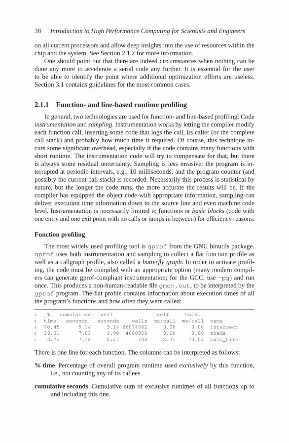
38 Introduction to High Performance Computing for Scientists and Engineers
on all current processors and allow deep insights into the use of resources within thechip and the system. See Section 2.1.2 for more information.
One should point out that there are indeed circumstances when nothing can bedone any more to accelerate a serial code any further. It is essential for the userto be able to identify the point where additional optimization efforts are useless.Section 3.1 contains guidelines for the most common cases.
2.1.1 Function- and line-based runtime profiling
In general, two technologies are used for function- and line-based profiling: Codeinstrumentation and sampling. Instrumentation works by letting the compiler modifyeach function call, inserting some code that logs the call, its caller (or the completecall stack) and probably how much time it required. Of course, this technique in-curs some significant overhead, especially if the code contains many functions withshort runtime. The instrumentation code will try to compensate for that, but thereis always some residual uncertainty. Sampling is less invasive: the program is in-terrupted at periodic intervals, e.g., 10 milliseconds, and the program counter (andpossibly the current call stack) is recorded. Necessarily this process is statistical bynature, but the longer the code runs, the more accurate the results will be. If thecompiler has equipped the object code with appropriate information, sampling candeliver execution time information down to the source line and even machine codelevel. Instrumentation is necessarily limited to functions or basic blocks (code withone entry and one exit point with no calls or jumps in between) for efficiency reasons.
Function profiling
The most widely used profiling tool is gprof from the GNU binutils package.gprof uses both instrumentation and sampling to collect a flat function profile aswell as a callgraph profile, also called a butterfly graph. In order to activate profil-ing, the code must be compiled with an appropriate option (many modern compil-ers can generate gprof-compliant instrumentation; for the GCC, use -pg) and runonce. This produces a non-human-readable file gmon.out, to be interpreted by thegprof program. The flat profile contains information about execution times of allthe program’s functions and how often they were called:
1 % cumulative self self total
2 time seconds seconds calls ms/call ms/call name
3 70.45 5.14 5.14 26074562 0.00 0.00 intersect
4 26.01 7.03 1.90 4000000 0.00 0.00 shade
5 3.72 7.30 0.27 100 2.71 73.03 calc_tile
There is one line for each function. The columns can be interpreted as follows:
% time Percentage of overall program runtime used exclusively by this function,i.e., not counting any of its callees.
cumulative seconds Cumulative sum of exclusive runtimes of all functions up toand including this one.

Basic optimization techniques for serial code 39
self seconds Number of seconds used by this function (exclusive). By default, thelist is sorted according to this field.
calls The number of times this function was called.
self ms/call Average number of milliseconds per call that were spent in this function(exclusive).
total ms/call Average number of milliseconds per call that were spent in this func-tion, including its callees (inclusive).
In the example above, optimization attempts would definitely start with theintersect() function, and shade() would also deserve a closer look. The cor-responding exclusive percentages can hint at the maximum possible gain. If, e.g.,shade() could be optimized to become twice as fast, the whole program wouldrun in roughly 7.3−0.95 = 6.35 seconds, i.e., about 15% faster.
Note that the outcome of a profiling run can depend crucially on the ability of thecompiler to perform function inlining. Inlining is an optimization technique that re-places a function call by the body of the callee, reducing overhead (see Section 2.4.2for a more thorough discussion). If inlining is allowed, the profiler output may bestrongly distorted when some hot spot function gets inlined and its runtime is at-tributed to the caller. If the compiler/profiler combination has no support for correctprofiling of inlined functions, it may be required to disallow inlining altogether. Ofcourse, this may itself have some significant impact on program performance char-acteristics.
A flat profile already contains a lot of information, however it does not revealhow the runtime contribution of a certain function is composed of several differentcallers, which other functions (callees) are called from it, and which contribution toruntime they in turn incur. This data is provided by the butterfly graph, or callgraph
profile:
1 index % time self children called name
2 0.27 7.03 100/100 main [2]
3 [1] 99.9 0.27 7.03 100 calc_tile [1]
4 1.90 5.14 4000000/4000000 shade [3]
5 -----------------------------------------------
6 <spontaneous>
7 [2] 99.9 0.00 7.30 main [2]
8 0.27 7.03 100/100 calc_tile [1]
9 -----------------------------------------------
10 5517592 shade [3]
11 1.90 5.14 4000000/4000000 calc_tile [1]
12 [3] 96.2 1.90 5.14 4000000+5517592 shade [3]
13 5.14 0.00 26074562/26074562 intersect [4]
14 5517592 shade [3]
15 -----------------------------------------------
16 5.14 0.00 26074562/26074562 shade [3]
17 [4] 70.2 5.14 0.00 26074562 intersect [4]
Each section of the callgraph pertains to exactly one function, which is listed to-gether with a running index (far left). The functions listed above this line are the

40 Introduction to High Performance Computing for Scientists and Engineers
current function’s callers, whereas those listed below are its callees. Recursive callsare accounted for (see the shade() function). These are the meanings of the variousfields:
% time The percentage of overall runtime spent in this function, including itscallees (inclusive time). This should be identical to the product of the num-ber of calls and the time per call on the flat profile.
self For each indexed function, this is exclusive execution time (identical to flat pro-file). For its callers (callees), it denotes the inclusive time this function (eachcallee) contributed to each caller (this function).
children For each indexed function, this is inclusive minus exclusive runtime, i.e.,the contribution of all its callees to inclusive time. Part of this time contributesto inclusive runtime of each of the function’s callers and is denoted in the re-spective caller rows. The callee rows in this column designate the contributionof each callee’s callees to the function’s inclusive runtime.
called denotes the number of times the function was called (probably split into re-cursive plus nonrecursive contributions, as shown in case of shade() above).Which fraction of the number of calls came from each caller is shown in thecaller row, whereas the fraction of calls for each callee that was initiated fromthis function can be found in the callee rows.
There are tools that can represent the butterfly profile in a graphical way, making itpossible to browse the call tree and quickly find the “critical path,” i.e., the sequenceof functions (from the root to some leaf) that shows dominant inclusive contributionsfor all its elements.
Line-based profiling
Function profiling becomes useless when the program to be analyzed containslarge functions (in terms of code lines) that contribute significantly to overall run-time:
1 % cumulative self self total
2 time seconds seconds calls s/call s/call name
3 73.21 13.47 13.47 1 13.47 18.40 MAIN__
4 6.47 14.66 1.19 21993788 0.00 0.00 mvteil_
5 6.36 15.83 1.17 51827551 0.00 0.00 ran1_
6 6.25 16.98 1.15 35996244 0.00 0.00 gzahl_
Here the MAIN function in a Fortran program requires over 73% of overall runtimebut has about 1700 lines of code. If the hot spot in such functions cannot be found bysimple common sense, tools for line-based profiling should be used. Many products,free and commercial, exist that can perform this task to different levels of sophisti-cation. As an example we pick the open source profiling tool OProfile [T19], whichcan in some sense act as a replacement for gprof because it can do function-basedflat and butterfly profiles as well. With OProfile, the only prerequisite the binary has

Basic optimization techniques for serial code 41
to fulfill is that debug symbols must be included (usually this is accomplished by the-g compiler option). Any special instrumentation is not required. A profiling dae-mon must be started (usually with the rights of a super user), which subsequentlymonitors the whole computer and collects data about all running binaries. The usercan later extract information about a specific binary. Among other things, this can bean annotated source listing in which each source line is accompanied by the numberof sampling hits (first column) and the relative percentage of total program samples(second column):
1 : DO 215 M=1,3
2 4292 0.9317 : bremsdir(M) = bremsdir(M) + FH(M)*Z12
3 1462 0.3174 : 215 CONTINUE
4 :
5 682 0.1481 : U12 = U12 + GCL12 * Upot
6 :
7 : DO 230 M=1,3
8 3348 0.7268 : F(M,I)=F(M,I)+FH(M)*Z12
9 1497 0.3250 : Fion(M)=Fion(M)+FH(M)*Z12
10 501 0.1088 :230 CONTINUE
This kind of data has to be taken with a grain of salt, though. The compiler-generatedsymbol tables must be consistent so that a machine instruction’s address in memorycan be properly matched to the correct source line. Modern compilers can reorganizecode heavily if high optimization levels are enabled. Loops can be fused or split,lines rearranged, variables optimized away, etc., so that the actual code executedmay be far from resembling the original source. Furthermore, due to the stronglypipelined architecture of modern microprocessors it is usually impossible to attributea specific moment in time to a particular source line or even machine instruction.However, looking at line-based profiling data on a loop-by-loop basis (samples inte-grated across the loop body) is relatively safe; in case of doubt, recompilation with alower optimization level (and inlining disabled) may provide more insight.
Above source line profile can be easily put into a form that allows identificationof hot spots. The cumulative sum over all samples versus source line number has asteep slope wherever many sampling hits are aggregated (see Figure 2.1).
2.1.2 Hardware performance counters
The first step in performance profiling is concerned with pinpointing the hot spotsin terms of runtime, i.e., clock ticks. But when it comes to identifying the actualreason for a code to be slow, or if one merely wants to know by which resource itis limited, clock ticks are insufficient. Luckily, modern processors feature a smallnumber of performance counters (often far less than ten), which are special on-chipregisters that get incremented each time a certain event occurs. Among the usuallyseveral hundred events that can be monitored, there are a few that are most useful forprofiling:
• Number of bus transactions, i.e., cache line transfers. Events like “cachemisses” are commonly used instead of bus transactions, however one should

42 Introduction to High Performance Computing for Scientists and Engineers
1000 1500 2000 2500source line #
0
5 k
10 k
15 k
20 k
sam
ple
s samples
cumulative sum (/20)
MAIN function subroutines
Figure 2.1: Sampling histogram (solid) with number of samples vs. source code line number.Dashed line: Cumulative sum over samples. Important hot spots (about 50% of overall time)are around line 1000 of the MAIN function, which encompasses over 1700 lines of code.
be aware that prefetching mechanisms (in hardware or software) can interferewith the number of cache misses counted. In that respect, bus transactions areoften the safer way to account for the actual data volume transferred over thememory bus. If the memory bandwidth used by a processor is close to thetheoretical maximum (or better, close to what standard low-level bandwidthbenchmarks like STREAM [W119, 134] can achieve; see Section 3.1), there isno point in trying to optimize further for better bus utilization. The number canalso be used for checking the correctness of some theoretical model one mayhave developed for estimating the data transfer requirements of an application(see Section 3.1 for an example of such a model).
• Number of loads and stores. Together with bus transactions, this can give anindication as to how efficiently cache lines are used for computation. If, e.g.,the number of DP loads and stores per cache line is less than its length in DPwords, this may signal strided memory access. One should however take intoaccount how the data is used; if, for some reason, the processor pipelines arestalled most of the time, or if many arithmetic operations on the data are per-formed out of registers, the strided access may not actually be a performancebottleneck.
• Number of floating-point operations. The importance of this very popular met-ric is often overrated. As will be shown in Chapter 3, data transfer is the dom-inant performance-limiting factor in scientific code. Even so, if the number

Basic optimization techniques for serial code 43
of floating-point operations per clock cycle is somewhere near the theoreticalmaximum (either given by the CPU’s peak performance, or less if there is anasymmetry between MULT and ADD operations), standard code optimizationis unlikely to achieve any improvement and algorithmic changes are probablyin order.
• Mispredicted branches. This counter is incremented when the CPU has pre-dicted the outcome of a conditional branch and the prediction has proved to bewrong. Depending on the architecture, the penalty for a mispredicted branchcan be tens of cycles (see Section 2.3.2 below). In general, scientific codestend to be loop-based so that branches are well predictable. However, “pointerchasing” and computed branches increase the probability of mispredictions.
• Pipeline stalls. Dependencies between operations running in different stagesof the processor pipeline (see Section 1.2.3) can lead to cycles during whichnot all stages are busy, so-called stalls or bubbles. Often bubbles cannot beavoided, e.g., when performance is limited by memory bandwidth and thearithmetic units spend their time waiting for data. Hence, it is quite difficultto identify the point where there are “too many” bubbles. Stall cycle anal-ysis is especially important on in-order architectures (like, e.g., Intel IA64)because bubbles cannot be filled by the hardware if there are no provisions forexecuting instructions that appear later in the instruction stream but have theiroperands available.
• Number of instructions executed. Together with clock cycles, this can be aguideline for judging how effectively the superscalar hardware with its mul-tiple execution units is utilized. Experience shows that it is quite hard forcompiler-generated code to reach more than 2–3 instructions per cycle, evenin tight inner loops with good pipelining properties.
There are essentially two ways to use hardware counters in profiling. In order to geta quick overview of the performance properties of an application, a simple tool canmeasure overall counts from start to finish and probably calculate some derived met-
rics like “instructions per cycle” or “cache misses per load or store.” A typical outputof such a tool could look like this if run with some application code (these exampleswere compiled from output generated by the lipfpm tool, which is delivered withsome SGI Altix systems):
1 CPU Cycles.............................................. 8721026107
2 Retired Instructions.................................... 21036052778
3 Average number of retired instructions per cycle........ 2.398151
4 L2 Misses............................................... 101822
5 Bus Memory Transactions................................. 54413
6 Average MB/s requested by L2............................ 2.241689
7 Average Bus Bandwidth (MB/s)............................ 1.197943
8 Retired Loads........................................... 694058538
9 Retired Stores.......................................... 199529719
10 Retired FP Operations................................... 7134186664
11 Average MFLOP/s......................................... 1225.702566
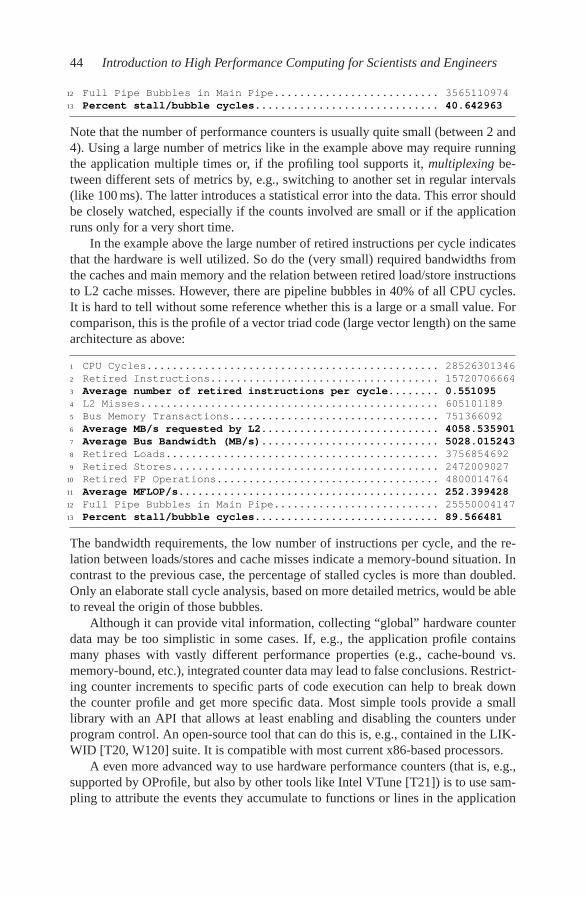
44 Introduction to High Performance Computing for Scientists and Engineers
12 Full Pipe Bubbles in Main Pipe.......................... 3565110974
13 Percent stall/bubble cycles............................. 40.642963
Note that the number of performance counters is usually quite small (between 2 and4). Using a large number of metrics like in the example above may require runningthe application multiple times or, if the profiling tool supports it, multiplexing be-tween different sets of metrics by, e.g., switching to another set in regular intervals(like 100 ms). The latter introduces a statistical error into the data. This error shouldbe closely watched, especially if the counts involved are small or if the applicationruns only for a very short time.
In the example above the large number of retired instructions per cycle indicatesthat the hardware is well utilized. So do the (very small) required bandwidths fromthe caches and main memory and the relation between retired load/store instructionsto L2 cache misses. However, there are pipeline bubbles in 40% of all CPU cycles.It is hard to tell without some reference whether this is a large or a small value. Forcomparison, this is the profile of a vector triad code (large vector length) on the samearchitecture as above:
1 CPU Cycles.............................................. 28526301346
2 Retired Instructions.................................... 15720706664
3 Average number of retired instructions per cycle........ 0.551095
4 L2 Misses............................................... 605101189
5 Bus Memory Transactions................................. 751366092
6 Average MB/s requested by L2............................ 4058.535901
7 Average Bus Bandwidth (MB/s)............................ 5028.015243
8 Retired Loads........................................... 3756854692
9 Retired Stores.......................................... 2472009027
10 Retired FP Operations................................... 4800014764
11 Average MFLOP/s......................................... 252.399428
12 Full Pipe Bubbles in Main Pipe.......................... 25550004147
13 Percent stall/bubble cycles............................. 89.566481
The bandwidth requirements, the low number of instructions per cycle, and the re-lation between loads/stores and cache misses indicate a memory-bound situation. Incontrast to the previous case, the percentage of stalled cycles is more than doubled.Only an elaborate stall cycle analysis, based on more detailed metrics, would be ableto reveal the origin of those bubbles.
Although it can provide vital information, collecting “global” hardware counterdata may be too simplistic in some cases. If, e.g., the application profile containsmany phases with vastly different performance properties (e.g., cache-bound vs.memory-bound, etc.), integrated counter data may lead to false conclusions. Restrict-ing counter increments to specific parts of code execution can help to break downthe counter profile and get more specific data. Most simple tools provide a smalllibrary with an API that allows at least enabling and disabling the counters underprogram control. An open-source tool that can do this is, e.g., contained in the LIK-WID [T20, W120] suite. It is compatible with most current x86-based processors.
A even more advanced way to use hardware performance counters (that is, e.g.,supported by OProfile, but also by other tools like Intel VTune [T21]) is to use sam-pling to attribute the events they accumulate to functions or lines in the application

Basic optimization techniques for serial code 45
code, much in the same way as in line-based profiling. Instead of taking a snapshotof the instruction pointer or call stack at regular intervals, an overflow value is de-fined for each counter (or, more exactly, each metric). When the counter reaches thisvalue, an interrupt is generated and an IP or call stack sample is taken. Naturally,samples generated for a particular metric accumulate at places where the counterwas incremented most often, allowing the same considerations as above not for thewhole program but on a function and even code line basis. It should, however, beclear that a correct interpretation of results from counting hardware events requires aconsiderable amount of experience.
2.1.3 Manual instrumentation
If the overheads subjected to the application by standard compiler-based instru-mentation are too large, or if only certain parts of the code should be profiled inorder to get a less complex view on performance properties, manual instrumentationmay be considered. The programmer inserts calls to a a wallclock timing routinelike gettimeofday() (see Listing 1.2 for a convenient wrapper function) or, ifhardware counter information is required, a profiling library like PAPI [T22] into theprogram. Some libraries also allow to start and stop the standard profiling mecha-nisms as described in Sections 2.1.1 and 2.1.2 under program control [T20]. Thiscan be very interesting in C++ where standard profiles are often very cluttered dueto the use of templates and operator overloading.
The results returned by timing routines should be interpreted with some care. Themost frequent mistake with code timings occurs when the time periods to be mea-sured are in the same order of magnitude as the timer resolution, i.e., the minimumpossible interval that can be resolved.
2.2 Common sense optimizations
Very simple code changes can often lead to a significant performance boost. Themost important “common sense” guidelines regarding the avoidance of performancepitfalls are summarized in the following sections. Some of those hints may seem triv-ial, but experience shows that many scientific codes can be improved by the simplestof measures.
2.2.1 Do less work!
In all but the rarest of cases, rearranging the code such that less work than beforeis being done will improve performance. A very common example is a loop thatchecks a number of objects to have a certain property, but all that matters in the endis that any object has the property at all:

46 Introduction to High Performance Computing for Scientists and Engineers
1 logical :: FLAG
2 FLAG = .false.
3 do i=1,N
4 if(complex_func(A(i)) < THRESHOLD) then
5 FLAG = .true.
6 endif
7 enddo
If complex_func() has no side effects, the only information that gets communi-cated to the outside of the loop is the value of FLAG. In this case, depending on theprobability for the conditional to be true, much computational effort can be saved byleaving the loop as soon as FLAG changes state:
1 logical :: FLAG
2 FLAG = .false.
3 do i=1,N
4 if(complex_func(A(i)) < THRESHOLD) then
5 FLAG = .true.
6 exit
7 endif
8 enddo
2.2.2 Avoid expensive operations!
Sometimes, implementing an algorithm is done in a thoroughly “one-to-one”way, translating formulae to code without any reference to performance issues. Whilethis is actually good (performance optimization always bears the slight danger ofchanging numerics, if not results), in a second step all those operations should beeliminated that can be substituted by “cheaper” alternatives. Prominent examples forsuch “strong” operations are trigonometric functions or exponentiation. Bear in mindthat an expression like x**2.0 is often not optimized by the compiler to becomex*x but left as it stands, resulting in the evaluation of an exponential and a loga-rithm. The corresponding optimization is called strength reduction. Apart from thesimple case described above, strong operations sometimes appear with a limited setof fixed arguments. This is an example from a simulation code for nonequilibriumspin systems:
1 integer :: iL,iR,iU,iO,iS,iN
2 double precision :: edelz,tt
3 ... ! load spin orientations
4 edelz = iL+iR+iU+iO+iS+iN ! loop kernel
5 BF = 0.5d0*(1.d0+TANH(edelz/tt))
The last two lines are executed in a loop that accounts for nearly the whole run-time of the application. The integer variables store spin orientations (up or down,i.e., −1 or +1, respectively), so the edelz variable only takes integer values in therange {−6, . . . ,+6}. The tanh() function is one of those operations that take vastamounts of time (at least tens of cycles), even if implemented in hardware. In the case
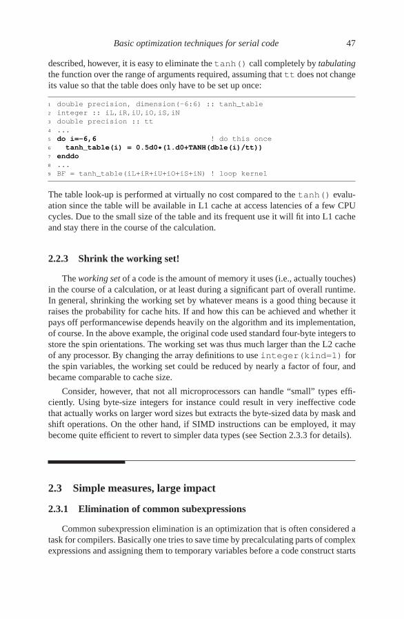
Basic optimization techniques for serial code 47
described, however, it is easy to eliminate the tanh() call completely by tabulating
the function over the range of arguments required, assuming that tt does not changeits value so that the table does only have to be set up once:
1 double precision, dimension(-6:6) :: tanh_table
2 integer :: iL,iR,iU,iO,iS,iN
3 double precision :: tt
4 ...
5 do i=-6,6 ! do this once
6 tanh_table(i) = 0.5d0*(1.d0+TANH(dble(i)/tt))
7 enddo
8 ...
9 BF = tanh_table(iL+iR+iU+iO+iS+iN) ! loop kernel
The table look-up is performed at virtually no cost compared to the tanh() evalu-ation since the table will be available in L1 cache at access latencies of a few CPUcycles. Due to the small size of the table and its frequent use it will fit into L1 cacheand stay there in the course of the calculation.
2.2.3 Shrink the working set!
The working set of a code is the amount of memory it uses (i.e., actually touches)in the course of a calculation, or at least during a significant part of overall runtime.In general, shrinking the working set by whatever means is a good thing because itraises the probability for cache hits. If and how this can be achieved and whether itpays off performancewise depends heavily on the algorithm and its implementation,of course. In the above example, the original code used standard four-byte integers tostore the spin orientations. The working set was thus much larger than the L2 cacheof any processor. By changing the array definitions to use integer(kind=1) forthe spin variables, the working set could be reduced by nearly a factor of four, andbecame comparable to cache size.
Consider, however, that not all microprocessors can handle “small” types effi-ciently. Using byte-size integers for instance could result in very ineffective codethat actually works on larger word sizes but extracts the byte-sized data by mask andshift operations. On the other hand, if SIMD instructions can be employed, it maybecome quite efficient to revert to simpler data types (see Section 2.3.3 for details).
2.3 Simple measures, large impact
2.3.1 Elimination of common subexpressions
Common subexpression elimination is an optimization that is often considered atask for compilers. Basically one tries to save time by precalculating parts of complexexpressions and assigning them to temporary variables before a code construct starts

48 Introduction to High Performance Computing for Scientists and Engineers
that uses those parts multiple times. In case of loops, this optimization is also calledloop invariant code motion:
1 ! inefficient
2 do i=1,N
3 A(i)=A(i)+s+r*sin(x)
4 enddo
−→tmp=s+r*sin(x)
do i=1,N
A(i)=A(i)+tmp
enddo
A lot of compute time can be saved by this optimization, especially where “strong”operations (like sin()) are involved. Although it may happen that subexpressionsare obstructed by other code and not easily recognizable, compilers are in princi-ple able to detect this situation. They will, however, often refrain from pulling thesubexpression out of the loop if this required employing associativity rules (see Sec-tion 2.4.4 for more information about compiler optimizations and reordering of arith-metic expressions). In practice, a good strategy is to help the compiler by eliminatingcommon subexpressions by hand.
2.3.2 Avoiding branches
“Tight” loops, i.e., loops that have few operations in them, are typical candidatesfor software pipelining (see Section 1.2.3), loop unrolling, and other optimizationtechniques (see below). If for some reason compiler optimization fails or is inef-ficient, performance will suffer. This can easily happen if the loop body containsconditional branches:
1 do j=1,N
2 do i=1,N
3 if(i.ge.j) then
4 sign=1.d0
5 else if(i.lt.j) then
6 sign=-1.d0
7 else
8 sign=0.d0
9 endif
10 C(j) = C(j) + sign * A(i,j) * B(i)
11 enddo
12 enddo
In this multiplication of a matrix with a vector, the upper and lower triangular partsget different signs and the diagonal is ignored. The if statement serves to decideabout which factor to use. Each time a corresponding conditional branch is encoun-tered by the processor, some branch prediction logic tries to guess the most probableoutcome of the test before the result is actually available, based on statistical meth-ods. The instructions along the chosen path are then fetched, decoded, and generallyfed into the pipeline. If the anticipation turns out to be false (this is called a mis-
predicted branch or branch miss), the pipeline has to be flushed back to the positionof the branch, implying many lost cycles. Furthermore, the compiler refrains fromdoing advanced optimizations like unrolling or SIMD vectorization (see the follow-

Basic optimization techniques for serial code 49
ing section). Fortunately, the loop nest can be transformed so that all if statementsvanish:
1 do j=1,N
2 do i=j+1,N
3 C(j) = C(j) + A(i,j) * B(i)
4 enddo
5 enddo
6 do j=1,N
7 do i=1,j-1
8 C(j) = C(j) - A(i,j) * B(i)
9 enddo
10 enddo
By using two different variants of the inner loop, the conditional has effectively beenmoved outside. One should add that there is more optimization potential in this loopnest. Please consider Chapter 3 for more information on optimizing data access.
2.3.3 Using SIMD instruction sets
Although vector processors also use SIMD instructions and the use of SIMD inmicroprocessors is often termed “vectorization,” it is more similar to the multitrackproperty of modern vector systems. Generally speaking, a “vectorizable” loop in thiscontext will run faster if more operations can be performed with a single instruction,i.e., the size of the data type should be as small as possible. Switching from DP to SPdata could result in up to a twofold speedup (as is the case for the SIMD capabilitiesof x86-type CPUs [V104, V105]), with the additional benefit that more items fit intothe cache.
Certainly, preferring SIMD instructions over scalar ones is no guarantee for aperformance improvement. If the code is strongly limited by memory bandwidth, noSIMD technique can bridge this gap. Register-to-register operations will be greatlyaccelerated, but this will only lengthen the time the registers wait for new data fromthe memory subsystem.
In Figure 1.8, a single precision ADD instruction was depicted that might be usedin an array addition loop:
1 real, dimension(1:N) :: r, x, y
2 do i=1, N
3 r(i) = x(i) + y(i)
4 enddo
All iterations in this loop are independent, there is no branch in the loop body, andthe arrays are accessed with a stride of one. However, the use of SIMD requiressome rearrangement of a loop kernel like the one above to be applicable: A numberof iterations equal to the SIMD register size has to be executed as a single “chunk”without any branches in between. This is actually a well-known optimization thatcan pay off even without SIMD and is called loop unrolling (see Section 3.5 formore details outside the SIMD context). Since the overall number of iterations isgenerally not a multiple of the register size, some remainder loop is left to execute

50 Introduction to High Performance Computing for Scientists and Engineers
in scalar mode. In pseudocode, and ignoring software pipelining (see Section 1.2.3),this could look like the following:
1 ! vectorized part
2 rest = mod(N,4)
3 do i=1,N-rest,4
4 load R1 = [x(i),x(i+1),x(i+2),x(i+3)]
5 load R2 = [y(i),y(i+1),y(i+2),y(i+3)]
6 ! "packed" addition (4 SP flops)
7 R3 = ADD(R1,R2)
8 store [r(i),r(i+1),r(i+2),r(i+3)] = R3
9 enddo
10 ! remainder loop
11 do i=N-rest+1,N
12 r(i) = x(i) + y(i)
13 enddo
R1, R2, and R3 denote 128-bit SIMD registers here. In an optimal situation all thisis carried out by the compiler automatically. Compiler directives can be used to givehints as to where vectorization is safe and/or beneficial.
The SIMD load and store instructions suggested in this example might need somespecial care. Some SIMD instruction sets distinguish between aligned and unaligned
data. For example, in the x86 (Intel/AMD) case, the “packed” SSE load and storeinstructions exist in aligned and unaligned flavors [V107, O54]. If an aligned load orstore is used on a memory address that is not a multiple of 16, an exception occurs.In cases where the compiler knows nothing about the alignment of arrays used in avectorized loop and cannot otherwise influence it, unaligned (or a sequence of scalar)loads and stores must be used, incurring some performance penalty. The programmercan force the compiler to assume optimal alignment, but this is dangerous if onecannot make absolutely sure that the assumption is justified. On some architecturesalignment issues can be decisive; every effort must then be made to align all loadsand stores to the appropriate address boundaries.
A loop with a true dependency as discussed in Section 1.2.3 cannot be SIMD-vectorized in this way (there is a twist to this, however; see Problem 2.2):
1 do i=2,N
2 A(i)=s*A(i-1)
3 enddo
The compiler will revert to scalar operations here, which means that only the lowestoperand in the SIMD registers is used (on x86 architectures).
Note that there are no fixed guidelines for when a loop qualifies as vectorized.One (maybe the weakest) possible definition is that all arithmetic within the loop isexecuted using the full width of SIMD registers. Even so, the load and store instruc-tions could still be scalar; compilers tend to report such loops as “vectorized” as well.On x86 processors with SSE support, the lower and higher 64 bits of a register canbe moved independently. The vector addition loop above could thus look as followsin double precision:

Basic optimization techniques for serial code 51
1 rest = mod(N,2)
2 do i=1,N-rest,2
3 ! scalar loads
4 load R1.low = x(i)
5 load R1.high = x(i+1)
6 load R2.low = y(i)
7 load R2.high = y(i+1)
8 ! "packed" addition (2 DP flops)
9 R3 = ADD(R1,R2)
10 ! scalar stores
11 store r(i) = R3.low
12 store r(i+1) = R3.high
13 enddo
14 ! remainder "loop"
15 if(rest.eq.1) r(N) = x(N) + y(N)
This version will not give the best performance if the operands reside in a cache.Although the actual arithmetic operations (line 9) are SIMD-parallel, all loads andstores are scalar. Lacking extensive compiler reports, the only option to identify sucha failure is manual inspection of the generated assembly code. If the compiler cannotbe convinced to properly vectorize a loop even with additional command line optionsor source code directives, a typical “last resort” before using assembly language al-together is to employ compiler intrinsics. Intrinsics are constructs that resemble as-sembly instructions so closely that they can usually be translated 1:1 by the compiler.However, the user is relieved from the burden of keeping track of individual regis-ters, because the compiler provides special data types that map to SIMD operands.Intrinsics are not only useful for vectorization but can be beneficial in all cases wherehigh-level language constructs cannot be optimally mapped to some CPU function-ality. Unfortunately, intrinsics are usually not compatible across compilers even onthe same architecture [V112].
Finally, it must be stressed that in contrast to real vector processors, RISC sys-tems will not always benefit from vectorization. If a memory-bound code can beoptimized for heavy data reuse from registers or cache (see Chapter 3 for examples),the potential gains are so huge that it may be acceptable to give up vectorizabilityalong the way.
2.4 The role of compilers
Most high-performance codes benefit, to varying degrees, from employingcompiler-based optimizations. Every modern compiler has command line switchesthat allow a (more or less) fine-grained tuning of the available optimization options.Sometimes it is even worthwhile trying a different compiler just to check whetherthere is more performance potential. One should be aware that the compiler has theextremely complex job of mapping source code written in a high-level language tomachine code, thereby utilizing the processor’s internal resources as well as possi-

52 Introduction to High Performance Computing for Scientists and Engineers
ble. Some of the optimizations described in this and the next chapter can be appliedby the compiler itself in simple situations. However, there is no guarantee that thisis actually the case and the programmer should at least be aware of the basic strate-gies for automatic optimization and potential stumbling blocks that prevent the latterfrom being applied. It must be understood that compilers can be surprisingly smartand stupid at the same time. A common statement in discussions about compiler ca-pabilities is “The compiler should be able to figure that out.” This is often enough afalse assumption.
Ref. [C91] provides a comprehensive overview on optimization capabilities ofseveral current C/C++ compilers, together with useful hints and guidelines for man-ual optimization.
2.4.1 General optimization options
Every compiler offers a collection of standard optimization options (-O0,-O1,. . . ). What kinds of optimizations are employed at which level is by no meansstandardized and often (but not always) documented in the manuals. However, allcompilers refrain from most optimizations at level -O0, which is hence the correctchoice for analyzing the code with a debugger. At higher levels, optimizing compilersmix up source lines, detect and eliminate “redundant” variables, rearrange arithmeticexpressions, etc., so that any debugger has a hard time giving the user a consistentview on code and data.
Unfortunately, some problems seem to appear only with higher optimization lev-els. This might indicate a defect in the compiler, however it is also possible that atypical bug like an array bounds violation (reading or writing beyond the bound-aries of an array) is “harmless” at -O0 because data is arranged differently than at-O3. Such bugs are notoriously hard to spot, and sometimes even the popular “printfdebugging” does not help because it interferes with the optimizer.
2.4.2 Inlining
Inlining tries to save overhead by inserting the complete code of a function orsubroutine at the place where it is called. Each function call uses up resources be-cause arguments have to be passed, either in registers or via the stack (dependingon the number of parameters and the calling conventions used). While the scope ofthe former function (local variables, etc.) must be established anyway, inlining doesremove the necessity to push arguments onto the stack and enables the compiler touse registers as it deems necessary (and not according to some calling convention),thereby reducing register pressure. Register pressure occurs if the CPU does not haveenough registers to hold all the required operands inside a complex computation orloop body (see also Section 2.4.5 for more information on register usage). And fi-nally, inlining a function allows the compiler to view a larger portion of code andprobably employ optimizations that would otherwise not be possible. The program-mer should never rely on the compiler to optimize inlined code perfectly, though; in

Basic optimization techniques for serial code 53
performance-critical situations (like tight loop kernels), obfuscating the compiler’sview on the “real” code is usually counterproductive.
Whether the call overhead impacts performance depends on how much time isspent in the function body itself; naturally, frequently called small functions bearthe highest speedup potential if inlined. In many C++ codes, inlining is absolutelyessential to get good performance because overloaded operators for simple types tendto be small functions, and temporary copies can be avoided if an inlined functionreturns an object (see Section 2.5 for details on C++ optimization).
Compilers usually have various options to control the extent of automatic inlin-ing, e.g., how large (in terms of the number of lines) a subroutine may be to becomean inlining candidate, etc. Note that the c99 and C++ inline keyword is only a hintto the compiler. A compiler log (if available, see Section 2.4.6) should be consultedto see whether a function was really inlined.
On the downside, inlining a function in multiple places can enlarge the objectcode considerably, which may lead to problems with L1 instruction cache capacity. Ifthe instructions belonging to a loop cannot be fetched from L1I cache, they competewith data transfers to and from outer-level cache or main memory, and the latencyfor fetching instructions becomes larger. Thus one should be cautious about alteringthe compiler’s inlining heuristics, and carefully check the effectiveness of manualinterventions.
2.4.3 Aliasing
The compiler, guided by the rules of the programming language and its inter-pretation of the source, must make certain assumptions that may limit its ability togenerate optimal machine code. The typical example arises with pointer (or refer-ence) formal parameters in the C (and C++) language:
1 void scale_shift(double *a, double *b, double s, int n) {
2 for(int i=1; i<n; ++i)
3 a[i] = s*b[i-1];
4 }
Assuming that the memory regions pointed to by a and b do not overlap, i.e., theranges [a,a+n−1] and [b,b+n−1] are disjoint, the loads and stores in the loop canbe arranged in any order. The compiler can apply any software pipelining schemeit considers appropriate, or it could unroll the loop and group loads and stores inblocks, as shown in the following pseudocode (we ignore the remainder loop):
1 loop:
2 load R1 = b(i+1)
3 load R2 = b(i+2)
4 R1 = MULT(s,R1)
5 R2 = MULT(s,R2)
6 store a(i) = R1
7 store a(i+1) = R2
8 i = i + 2
9 branch -> loop

54 Introduction to High Performance Computing for Scientists and Engineers
In this form, the loop could easily be SIMD-vectorized as well (see Section 2.3.3).
However, the C and C++ standards allow for arbitrary aliasing of pointers. Itmust thus be assumed that the memory regions pointed to by a and b do overlap. Forinstance, if a==b, the loop is identical to the “real dependency” Fortran example onpage 12; loads and stores must be executed in the same order in which they appearin the code:
1 loop:
2 load R1 = b(i+1)
3 R1 = MULT(s,R1)
4 store a(i) = R1
5 load R2 = b(i+2)
6 R2 = MULT(s,R2)
7 store a(i+1) = R2
8 i = i + 2
9 branch -> loop
Lacking any further information, the compiler must generate machine instructionsaccording to this scheme. Among other things, SIMD vectorization is ruled out. Theprocessor hardware allows reordering of loads and stores within certain limits [V104,V105], but this can of course never alter the program’s semantics.
Argument aliasing is forbidden by the Fortran standard, and this is one of themain reasons why Fortran programs tend to be faster than equivalent C programs.All C/C++ compilers have command line options to control the level of aliasing thecompiler is allowed to assume (e.g., -fno-fnalias for the Intel compiler and-fargument-noalias for the GCC specify that no two pointer arguments forany function ever point to the same location). If the compiler is told that argumentaliasing does not occur, it can in principle apply the same optimizations as in equiva-lent Fortran code. Of course, the programmer should not “lie” in this case, as callinga function with aliased arguments will then probably produce wrong results.
2.4.4 Computational accuracy
As already mentioned in Section 2.3.1, compilers sometimes refrain from rear-ranging arithmetic expressions if this required applying associativity rules, exceptwith very aggressive optimizations turned on. The reason for this is the infamousnonassociativity of FP operations [135]: (a+b)+c is, in general, not identical toa+(b+c) if a, b, and c are finite-precision floating-point numbers. If accuracy is tobe maintained compared to nonoptimized code, associativity rules must not be usedand it is left to the programmer to decide whether it is safe to regroup expressionsby hand. Modern compilers have command line options that limit rearrangement ofarithmetic expressions even at high optimization levels.
Note also that denormals, i.e., floating-point numbers that are smaller than thesmallest representable number with a nonzero lead digit, can have a significant im-pact on computational performance. If possible, and if the slight loss in accuracy istolerable, such numbers should be treated as (“flushed to”) zero by the hardware.

Basic optimization techniques for serial code 55
Listing 2.1: Compiler log for a software pipelined triad loop. “Peak” indicates the maximumpossible execution rate for the respective operation type on this architecture (MIPS R14000).
1 #<swps> 16383 estimated iterations before pipelining
2 #<swps> 4 unrollings before pipelining
3 #<swps> 20 cycles per 4 iterations
4 #<swps> 8 flops ( 20% of peak) (madds count as 2)
5 #<swps> 4 flops ( 10% of peak) (madds count as 1)
6 #<swps> 4 madds ( 20% of peak)
7 #<swps> 16 mem refs ( 80% of peak)
8 #<swps> 5 integer ops ( 12% of peak)
9 #<swps> 25 instructions ( 31% of peak)
10 #<swps> 2 short trip threshold
11 #<swps> 13 integer registers used.
12 #<swps> 17 float registers used.
2.4.5 Register optimizations
It is one of the most vital, but also most complex tasks of the compiler to careabout register usage. The compiler tries to put operands that are used “most often”into registers and keep them there as long as possible, given that it is safe to do so.If, e.g., a variable’s address is taken, its value might be manipulated elsewhere inthe program via the address. In this case the compiler may decide to write a variableback to memory right after any change on it.
Inlining (see Section 2.4.2) will help with register optimizations since the opti-mizer can probably keep values in registers that would otherwise have to be writtento memory before the function call and read back afterwards. On the downside, loopbodies with lots of variables and many arithmetic expressions (which can easily oc-cur after inlining) are hard for the compiler to optimize because it is likely that thereare too few registers to hold all operands at the same time. As mentioned earlier, thenumber of integer and floating-point registers in any processor is strictly limited. To-day, typical numbers range from 8 to 128, the latter being a gross exception, however.If there is a register shortage, variables have to be spilled, i.e., written to memory, forlater use. If the code’s performance is determined by arithmetic operations, registerspill can hamper performance quite a bit. In such cases it may even be worthwhilesplitting a loop in two to reduce register pressure.
Some processors with hardware support for spilling like, e.g., Intel’s Itanium2,feature hardware performance counter metrics, which allow direct identification ofregister spill.
2.4.6 Using compiler logs
The previous sections have pointed out that the compiler is a crucial compo-nent in writing efficient code. It is very easy to hide important information from thecompiler, forcing it to give up optimization at an early stage. In order to make thedecisions of the compiler’s “intelligence” available to the user, many compilers offer

56 Introduction to High Performance Computing for Scientists and Engineers
options to generate annotated source code listings or at least logs that describe insome detail what optimizations were performed. Listing 2.1 shows an example for acompiler annotation regarding a standard vector triad loop as in Listing 1.1, for the(now outdated) MIPS R14000 processor. This CPU was four-way superscalar, withthe ability to execute one load or store, two integer, one FP add and one FP multiplyoperation per cycle (the latter two in the form of a fused multiply-add [“madd”] in-struction). Assuming that all data is available from the inner level cache, the compilercan calculate the minimum number of cycles required to execute one loop iteration(line 3). Percentages of Peak, i.e., the maximum possible throughput for every typeof operation, are indicated in lines 4–9.
Additionally, information about register usage and spill (lines 11 and 12), un-rolling factors and software pipelining (line 2, see Sections 1.2.3 and 3.5), use ofSIMD instructions (see Section 2.3.3), and the compiler’s assumptions about looplength (line 1) are valuable for judging the quality of generated machine code. Un-fortunately, not all compilers have the ability to write such comprehensive code an-notations and users are often left with guesswork.
Certainly there is always the option of manually inspecting the generated assem-bly code. All compilers provide command line options to output an assembly listinginstead of a linkable object file. However, matching this listing with the originalsource code and analyzing the effectiveness of the instruction sequences requires aconsiderable amount of experience [O55]. After all there is a reason for people notwriting programs in assembly language all the time.
2.5 C++ optimizations
There is a host of literature dealing with how to write efficient C++ code [C92,C93, C94, C95], and it is not our ambition to supersede it here. We also deliberatelyomit standard techniques like reference counting, copy-on-write, smart pointers, etc.In this section we will rather point out, in our experience, the most common perfor-mance bugs and misconceptions in C++ programs, with a focus on low-level loops.
One of the ineradicable illusions about C++ is that the compiler should be able tosee through all the abstractions and obfuscations an “advanced” C++ program con-tains. First and foremost, C++ should be seen as a language that enables complex-
ity management. The features one has grown fond of in this concept, like operatoroverloading, object orientation, automatic construction/destruction, etc., are howevermostly unsuitable for efficient low-level code.
2.5.1 Temporaries
C++ fosters an “implicit” programming style where automatic mechanisms hidecomplexity from the programmer. A frequent problem occurs with expressions con-taining chains of overloaded operators. As an example, assume there is a vec3d

Basic optimization techniques for serial code 57
class, which represents a vector in three-dimensional space. Overloaded arithmeticoperators then allow expressive coding:
1 class vec3d {
2 double x,y,z;
3 friend vec3d operator*(double, const vec3d&);
4 public:
5 vec3d(double _x=0.0, double _y=0.0, double _z=0.0) : // 4 ctors
6 x(_x),y(_y),z(_z) {}
7 vec3d(const vec3d &other);
8 vec3d operator=(const vec3d &other);
9 vec3d operator+(const vec3d &other) {
10 vec3d tmp;
11 tmp.x = x + other.x;
12 tmp.y = y + other.y;
13 tmp.z = z + other.z;
14 }
15 vec3d operator*(const vec3d &other);
16 ...
17 };
18
19 vec3d operator*(double s, const vec3d& v) {
20 vec3d tmp(s*v.x,s*v,y,s*v.z);
21 }
Here we show only the implementation of the vec3d::operator+ method andthe friend function for multiplication by a scalar. Other useful functions are definedin a similar way. Note that copy constructors and assignment are shown for referenceas prototypes, but are implicitly defined because shallow copy and assignment aresufficient for this simple class.
The following code fragment shall serve as an instructive example of what reallygoes on behind the scenes when a class is used:
1 vec3d a,b(2,2),c(3);
2 double x=1.0,y=2.0;
3
4 a = x*b + y*c;
In this example the following steps will occur (roughly) in this order:
1. Constructors for a, b, c, and d are called (the default constructor is imple-mented via default arguments to the parameterized constructor)
2. operator*(x, b) is called
3. The vec3d constructor is called to initialize tmp inoperator*(double s, const vec3d& v) (here we have al-ready chosen the more efficient three-parameter constructor instead of thedefault constructor followed by assignment from another temporary)
4. Since tmp must be destroyed onceoperator*(double, const vec3d&) returns, vec3d’s copy

58 Introduction to High Performance Computing for Scientists and Engineers
constructor is invoked to make a temporary copy of the result, to be used asthe first argument in the vector addition
5. operator*(y, c) is called
6. The vec3d constructor is called to initialize tmp inoperator*(double s, const vec3d& v)
7. Since tmp must be destroyed onceoperator*(double, const vec3d&) returns, vec3d’s copyconstructor is invoked to make a temporary copy of the result, to be used asthe second argument in the vector addition
8. vec3d::operator+(const vec3d&) is called in the first temporaryobject with the second as a parameter
9. vec3d’s default constructor is called to make tmp invec3d::operator+
10. vec3d’s copy constructor is invoked to make a temporary copy of the sum-mation’s result
11. vec3d’s assignment operator is called in a with the temporary result as itsargument
Although the compiler may eliminate the local tmp objects by the so-called return
value optimization [C92] using the required implicit temporary directly instead oftmp, it is striking how much code gets executed for this seemingly simple expres-sion (a debugger can help a lot with getting more insight here). A straightforwardoptimization, at the price of some readability, is to use compound computational/as-signment operators like operator+=:
1 a = y*c;
2 a += x*b;
Two temporaries are still required here to transport the results fromoperator*(double, const vec3d&) back into the main function, butthey are used in an assignment and vec3d::operator+= right away without theneed for a third temporary. The benefit is even more noticeable with longer operatorchains.
However, even if a lot of compute time is spent handling temporaries, callingcopy constructors, etc., this fact is not necessarily evident from a standard functionprofile like the ones shown in Section 2.1.1. C++ compilers are, necessarily, quitegood at function inlining. Much of the implicit “magic” going on could thus be sum-marized as, e.g., exclusive runtime of the function invoking a complex expression.Disabling inlining, although generally advised against, might help to get more insightin this situation, but it will distort the results considerably.
Despite aggressive inlining the compiler will most probably not generate “opti-mal” code, which would roughly look like this:
Basic optimization techniques for serial code 59
1 a.x = x*b.x + y*c.x;
2 a.y = x*b.y + y*c.y;
3 a.z = x*b.z + y*c.z;
Expression templates [C96, C97] are an advanced programming technique that cansupposedly lift many of the performance problems incurred by temporaries, and ac-tually produce code like this from high-level expressions.
It should nonetheless be clear that it is not the purpose of C++ inlining to producethe optimal code, but to rectify the most severe performance penalties incurred by thelanguage specification. Loop kernels bound by memory or even cache bandwidth,or arithmetic throughput, are best written either in C (or C style) or Fortran. SeeSection 2.5.3 for details.
2.5.2 Dynamic memory management
Another common bottleneck in C++ codes is frequent allocation and dealloca-tion. There was no dynamic memory involved in the simple 3D vector class exampleabove, so there was no problem with abundant (de)allocations. Had we chosen to usea general vector-like class with variable size, the performance implications of tem-poraries would have been even more severe, because construction and destruction ofeach temporary would have called malloc() and free(), respectively. Since thestandard library functions are not optimized for minimal overhead, this can seriouslyharm overall performance. This is why C++ programmers go to great lengths tryingto reduce the impact of allocation and deallocation [C98].
Avoiding temporaries is of course one of the key measures here (see the previ-ous section), but two other strategies are worth noting: Lazy construction and static
construction. These two seem somewhat contrary, but both have useful applications.
Lazy construction
For C programmers who adopted C++ as a “second language” it is natural to col-lect object declarations at the top of a function instead of moving each declaration tothe place where it is needed. The former is required by C, and there is no performanceproblem with it as long as only basic data types are used. An expensive constructorshould be avoided as far as possible, however:
1 void f(double threshold, int length) {
2 std::vector<double> v(length);
3 if(rand() > threshold*RAND_MAX) {
4 v = obtain_data(length);
5 std::sort(v.begin(), v.end());
6 process_data(v);
7 }
8 }
In line 2, construction of v is done unconditionally although the probability that itis really needed might be low (depending on threshold). A better solution is todefer construction until this decision has been made:
60 Introduction to High Performance Computing for Scientists and Engineers
1 void f(double threshold, int length) {
2 if(rand() > threshold*RAND_MAX) {
3 std::vector<double> v(obtain_data(length));
4 std::sort(v.begin(), v.end());
5 process_data(v);
6 }
7 }
As a positive side effect we now call the copy constructor of std::vector<>(line 3) instead of the int constructor followed by an assignment.
Static construction
Moving the construction of an object to the outside of a loop or block, or mak-ing it static altogether, may even be faster than lazy construction if the object isused often. In the example above, if the array length is constant and threshold
is usually close to 1, static allocation will make sure that construction overhead isnegligible since it only has to be paid once:
1 const int length=1000;
2
3 void f(double threshold) {
4 static std::vector<double> v(length);
5 if(rand() > threshold*RAND_MAX) {
6 v = obtain_data(length);
7 std::sort(v.begin(), v.end());
8 process_data(v);
9 }
10 }
The vector object is instantiated only once in line 4, and there is no subsequent al-location overhead. With a variable length there is the chance that memory wouldhave to be re-allocated upon assignment, incurring the same cost as a normal con-structor (see also Problem 2.4). In general, if assignment is faster (on average) than(re-)allocation, static construction will be faster.
Note that special care has to be taken of static data in shared-memory parallelprograms; see Section 6.1.4 for details.
2.5.3 Loop kernels and iterators
The runtime of scientific applications tends to be dominated by loops or loopnests, and the compiler’s ability to optimize those loops is pivotal for getting goodcode performance. Operator overloading, convenient as it may be, hinders good loopoptimization. In the following example, the template function sprod<>() is re-sponsible for carrying out a scalar product over two vectors:
1 using namespace std;
2
3 template<class T> T sprod(const vector<T> &a, const vector<T> &b) {
4 T result=T(0);

Basic optimization techniques for serial code 61
5 int s = a.size();
6 for(int i=0; i<s; ++i) // not SIMD vectorized
7 result += a[i] * b[i];
8 return result;
9 }
In line 7, const T& vector<T>::operator[] is called twice to obtain thecurrent entries from a and b. STL may define this operator in the following way(adapted from the GNU ISO C++ library source):
1 const T& operator[](size_t __n) const
2 { return *(this->_M_impl._M_start + __n); }
Although this looks simple enough to be inlined efficiently, current compilers refuseto apply SIMD vectorization to the summation loop above. A single layer of ab-straction, in this case an overloaded index operator, can thus prevent the creation ofoptimal loop code (and we are not even referring to more complex, high-level looptransformations like those described in Chapter 3). However, using iterators for arrayaccess, vectorization is not a problem:
1 template<class T> T sprod(const vector<T> &a, const vector<T> &b) {
2 typename vector<T>::const_iterator ia=a.begin(),ib=b.begin();
3 T result=T(0);
4 int s = a.size();
5 for(int i=0; i<s; ++i) // SIMD vectorized
6 result += ia[i] * ib[i];
7 return result;
8 }
Because vector<T>::const_iterator is const T*, the compiler sees nor-mal C code. The use of iterators instead of methods for data access can be a powerfuloptimization method in C++. If possible, low-level loops should even reside in sepa-rate compilation units (and written in C or Fortran), and iterators be passed as point-ers. This ensures minimal interference with the compiler’s view on the high-levelC++ code.
The std::vector<> template is a particularly rewarding case because its iter-ators are implemented as standard (C) pointers, but it is also the most frequently usedcontainer. More complex containers have more complex iterator classes, and thosemay not be easily convertible to raw pointers. In cases where it is possible to repre-sent data in a “segmented” structure with multiple vector<>-like components (amatrix being the standard example), the use of segmented iterators still enables fastlow-level algorithms. See [C99, C100] for details.

62 Introduction to High Performance Computing for Scientists and Engineers
Problems
For solutions see page 288 ff.
2.1 The perils of branching. Consider this benchmark code for a stride-one triad“with a twist”:
1 do i=1,N
2 if(C(i)<0.d0) then
3 A(i) = B(i) - C(i) * D(i)
4 else
5 A(i) = B(i) + C(i) * D(i)
6 endif
7 enddo
What performance impact do you expect from the conditional compared to thestandard vector triad if array C is initialized with (a) positive values only (b)negative values only (c) random values between −1 and 1 for loop lengths thatfit in L1 cache, L2 cache, and memory, respectively?
2.2 SIMD despite recursion? In Section 1.2.3 we have studied the influence ofloop-carried dependencies on pipelining using the following loop kernel:
1 start=max(1,1-offset)
2 end=min(N,N-offset)
3 do i=start,end
4 A(i)=s*A(i+offset)
5 enddo
If A is an array of single precision floating-point numbers, for which values ofoffset is SIMD vectorization as shown in Figure 1.8 possible?
2.3 Lazy construction on the stack. If we had used a standard C-style double ar-ray instead of a std::vector<double> for the lazy construction examplein Section 2.5.2, would it make a difference where it was declared?
2.4 Fast assignment. In the static construction example in Section 2.5.2 we statedthat the benefit of a static std::vector<> object can only be seen with aconstant vector length, because assignment leads to re-allocation if the lengthcan change. Is this really true?

Chapter 3
Data access optimization
Of all possible performance-limiting factors in HPC, the most important one is dataaccess. As explained earlier, microprocessors tend to be inherently “unbalanced”with respect to the relation of theoretical peak performance versus memory band-width. Since many applications in science and engineering consist of loop-basedcode that moves large amounts of data in and out of the CPU, on-chip resources tendto be underutilized and performance is limited only by the relatively slow data pathsto memory or even disks.
Figure 3.1 shows an overview of several data paths present in modern parallelcomputer systems, and typical ranges for their bandwidths and latencies. The func-tional units, which actually perform the computational work, sit at the top of thishierarchy. In terms of bandwidth, the slowest data paths are three to four orders ofmagnitude away, and eight in terms of latency. The deeper a data transfer must reachdown through the different levels in order to obtain required operands for some cal-culation, the harder the impact on performance. Any optimization attempt shouldtherefore first aim at reducing traffic over slow data paths, or, should this turn out tobe infeasible, at least make data transfer as efficient as possible.
3.1 Balance analysis and lightspeed estimates
3.1.1 Bandwidth-based performance modeling
Some programmers go to great lengths trying to improve the efficiency of code.In order to decide whether this makes sense or if the program at hand is alreadyusing the resources in the best possible way, one can often estimate the theoreticalperformance of loop-based code that is bound by bandwidth limitations by simplerules of thumb. The central concept to introduce here is balance. For example, themachine balance Bm of a processor chip is the ratio of possible memory bandwidthin GWords/sec to peak performance in GFlops/sec:
Bm =memory bandwidth [GWords/sec]peak performance [GFlops/sec]
=bmax
Pmax(3.1)
“Memory bandwidth” could also be substituted by the bandwidth to caches or evennetwork bandwidths, although the metric is generally most useful for codes that arereally memory-bound. Access latency is assumed to be hidden by techniques like
63

64 Introduction to High Performance Computing for Scientists and Engineers
10 11
10 10
10 9
10 8
10 7
−810
−710
−610
−910
−510
−410
−310
−210
−110
L1 cache
Main memory
L2/L3 cache
HPC networks
Gigabit Ethernet
Local hard disk
Internet
Solid state disk
BandwidthLatency
[sec] [bytes/sec]
Figure 3.1: Typical latency and bandwidth numbers for data transfer to and from differentdevices in computer systems. Registers have been omitted because their “bandwidth” usuallymatches the computational capabilities of the compute core, and their latency is part of thepipelined execution.

Data access optimization 65
data path balance [W/F]
cache 0.5–1.0
machine (memory) 0.03–0.5
interconnect (high speed) 0.001–0.02
interconnect (GBit ethernet) 0.0001–0.0007
disk (or disk subsystem) 0.0001–0.01
Table 3.1: Typical balance values for operations limited by different transfer paths. In caseof network and disk connections, the peak performance of typical dual-socket compute nodeswas taken as a basis.
prefetching and software pipelining. As an example, consider a dual-core chip witha clock frequency of 3.0 GHz that can perform at most four flops per cycle (per core)and has a memory bandwidth of 10.6 GBytes/sec. This processor would have a ma-chine balance of 0.055 W/F. At the time of writing, typical values of Bm lie in therange between 0.03 W/F for standard cache-based microprocessors and 0.5 W/F fortop of the line vector processors. Due to the continuously growing DRAM gap andthe increasing core counts, machine balance for standard architectures will presum-ably decrease further in the future. Table 3.1 shows typical balance values for severaldifferent transfer paths.
In Figure 3.2 we have collected peak performance and memory bandwidth datafor Intel processors between 1994 and 2010. Each year the desktop processor withthe fastest clock speed was chosen as a representative. Although peak performancedid grow faster than memory bandwidth before 2005, the introduction of the firstdual-core chip (Pentium D) really widened the DRAM gap considerably. The Corei7 design gained some ground in terms of bandwidth, but the long-term general trendis clearly unperturbed by such exceptions.
1994 1996 1998 2000 2002 2004 2006 2008 2010
Year
102
103
104
105
MF
lops/s
ec, M
Byte
s/s
ec Core 2 Duo 3.0
multicore
single-core
Peak bandwidth
Peak arithmeticperformance
P 200
P2 450
P3 600
P3 933
P4 1.7
P4 3.0
P4 3.4
Core 2 Quad 3.4
Core i7 3.2
Pentium D 3.6
Next gen.
Figure 3.2: Progressof maximum arithmeticperformance (open cir-cles) and peak theoreti-cal memory bandwidth(filled circles) for Intelprocessors since 1994.The fastest processor interms of clock frequencyis shown for each year.(Data collected by JanTreibig.)

66 Introduction to High Performance Computing for Scientists and Engineers
In order to quantify the requirements of some code that runs on a machine with acertain balance, we further define the code balance of a loop to be
Bc =data traffic [Words]
floating point ops [Flops]. (3.2)
“Data traffic” refers to all words transferred over the performance-limiting data path,which makes this metric to some extent dependent on the hardware (see Section 3.3for an example). The reciprocal of code balance is often called computational inten-
sity. We can now calculate the expected maximum fraction of peak performance of acode with balance Bc on a machine with balance Bm:
l = min
(
1,Bm
Bc
)
. (3.3)
We call this fraction the lightspeed of a loop. Performance in GFlops/sec is then
P = lPmax = min
(
Pmax,bmax
Bc
)
(3.4)
If l ≃ 1, performance is not limited by bandwidth but other factors, either inside theCPU or elsewhere. Note that this simple performance model is based on some crucialassumptions:
• The loop code makes use of all arithmetic units (MULT and ADD) in an opti-mal way. If this is not the case one must introduce a correction factor that re-flects the ratio of “effective” to absolute peak performance (e.g., if only ADDsare used in the code, effective peak performance would be half of the absolutemaximum). Similar considerations apply if less than the maximum number ofcores per chip are used.
• The loop code is based on double precision floating-point arithmetic. However,one can easily derive similar metrics that are more appropriate for other codes(e.g., 32-bit words per integer arithmetic instruction etc.).
• Data transfer and arithmetic overlap perfectly.
• The slowest data path determines the loop code’s performance. All faster datapaths are assumed to be infinitely fast.
• The system is in “throughput mode,” i.e., latency effects are negligible.
• It is possible to saturate the memory bandwidth that goes into the calculationof machine balance to its full extent. Recent multicore designs tend to under-utilize the memory interface if only a fraction of the cores use it. This makesperformance prediction more complex, since there is a separate “effective” ma-chine balance that is not just proportional to N−1 for each core count N. SeeSection 3.1.2 and Problem 3.1 below for more discussion regarding this point.

Data access optimization 67
type kernel DP words flops Bc
COPY A(:)=B(:) 2 (3) 0 N/A
SCALE A(:)=s*B(:) 2 (3) 1 2.0 (3.0)
ADD A(:)=B(:)+C(:) 3 (4) 1 3.0 (4.0)
TRIAD A(:)=B(:)+s*C(:) 3 (4) 2 1.5 (2.0)
Table 3.2: The STREAM benchmark kernels with their respective data transfer volumes (thirdcolumn) and floating-point operations (fourth column) per iteration. Numbers in brackets takewrite allocates into account.
While the balance model is often useful and accurate enough to estimate the perfor-mance of loop codes and get guidelines for optimization (especially if combined withvisualizations like the roofline diagram [M42]), we must emphasize that more ad-vanced strategies for performance modeling do exist and refer to the literature [L76,M43, M41].
As an example consider the standard vector triad benchmark introduced in Sec-tion 1.3. The kernel loop,
1 do i=1,N
2 A(i) = B(i) + C(i) * D(i)
3 enddo
executes two flops per iteration, for which three loads (to elements B(i), C(i), andD(i)) and one store operation (to A(i)) provide the required input data. The codebalance is thus Bc = (3 + 1)/2 = 2. On a CPU with machine balance Bm = 0.1, wecan then expect a lightspeed ratio of 0.05, i.e., 5% of peak.
Standard cache-based microprocessors usually have an outermost cache levelwith write-back strategy. As explained in Section 1.3, a cache line write allocateis then required after a store miss to ensure cache-memory coherence if nontemporalstores or cache line zero is not used. Under such conditions, the store stream to arrayA must be counted twice in calculating the code balance, and we would end up witha lightspeed estimate of lwa = 0.04.
3.1.2 The STREAM benchmarks
The McCalpin STREAM benchmarks [134, W119] is a collection of four simplesynthetic kernel loops which are supposed to fathom the capabilities of a processor’sor a system’s memory interface. Table 3.2 lists those operations with their respec-tive code balance. Performance is usually reported as bandwidth in GBytes/sec. TheSTREAM TRIAD kernel is not to be confused with the vector triad (see previoussection), which has one additional load stream.
The benchmarks exist in serial and OpenMP-parallel (see Chapter 6) variants andare usually run with data sets large enough so that performance is safely memory-bound. Measured bandwidth thus depends on the number of load and store streamsonly, and the results for COPY and SCALE (and likewise for ADD and TRIAD)

68 Introduction to High Performance Computing for Scientists and Engineers
tend to be very similar. One must be aware that STREAM is not only defined viathe loop kernels in Table 3.2, but also by its Fortran source code (there is also a Cvariant available). This is important because optimizing compilers can recognize theSTREAM source and substitute the kernels by hand-tuned machine code. Therefore,it is safe to state that STREAM performance results reflect the true capabilities of thehardware. They are published for many historical and contemporary systems on theSTREAM Web site [W119].
Unfortunately, STREAM as well as the vector triad often fail to reach the perfor-mance levels predicted by balance analysis, in particular on commodity (PC-based)hardware. The reasons for this failure are manifold and cannot be discussed here infull detail; typical factors are:
• Maximum bandwidth is often not available in both directions (read and write)concurrently. It may be the case, e.g., that the relation from maximum readto maximum write bandwidth is 2:1. A write stream cannot utilize the fullbandwidth in that case.
• Protocol overhead (see, e.g., Section 4.2.1), deficiencies in chipsets, error-correcting memory chips, and large latencies (that cannot be hidden com-pletely by prefetching) all cut on available bandwidth.
• Data paths inside the processor chip, e.g., connections between L1 cache andregisters, can be unidirectional. If the code is not balanced between read andwrite operations, some of the bandwidth in one direction is unused. This shouldbe taken into account when applying balance analysis for in-cache situations.
It is, however, still true that STREAM results mark a maximum for memory band-width and no real application code with similar characteristics (number of load andstore streams) performs significantly better. Thus, the STREAM bandwidth bS ratherthan the hardware’s theoretical capabilities should be used as the reference for light-speed calculations and (3.4) be modified to read
P = min
(
Pmax,bS
Bc
)
(3.5)
Getting a significant fraction (i.e., 80% or more) of the predicted performance basedon STREAM results for an application code is usually an indication that there isno more potential for improving the utilization of the memory interface. It does notmean, however, that there is no room for further optimizations. See the followingsections.
As an example we pick a system with Intel’s Xeon 5160 processor (see Figure 4.4for the general layout). One core has a theoretical memory bandwidth of bmax =10.66 GBytes/sec and a peak performance of Pmax = 12 GFlops/sec (4 flops per cycleat 3.0 GHz). This leads to a machine balance of Bm = 0.111 W/F for a single core(if both cores run memory-bound code, this is reduced by a factor of two, but weassume for now that only one thread is running on one socket of the system).
Table 3.3 shows the STREAM results on this platform, comparing versions with

Data access optimization 69
with write allocate w/o write allocate
type reported actual bS/bmax reported bS/bmax
COPY 2698 4047 0.38 4089 0.38
SCALE 2695 4043 0.38 4106 0.39
ADD 2772 3696 0.35 3735 0.35
TRIAD 2879 3839 0.36 3786 0.36
Table 3.3: Single-thread STREAM bandwidth results in GBytes/sec for an Intel Xeon 5160processor (see text for details), comparing versions with and without write allocate. Writeallocate was avoided by using nontemporal store instructions.
and without write allocate. The benchmark itself does not take this detail into ac-count at all, so reported bandwidth numbers differ from actual memory traffic ifwrite allocates are present. The discrepancy between measured performance and the-oretical maximum is very pronounced; it is generally not possible to get more than40% of peak bandwidth on this platform, and efficiency is particularly low for ADDand TRIAD, which have two load streams instead of one. If these results are usedas a reference for balance analysis of loops, COPY or SCALE should be used inload/store-balanced cases. See Section 3.3 for an example.
3.2 Storage order
Multidimensional arrays, first and foremost matrices or matrix-like structures,are omnipresent in scientific computing. Data access is a crucial topic here as themapping between the inherently one-dimensional, cache line based memory layoutof standard computers and any multidimensional data structure must be matched tothe order in which code loads and stores data so that spatial and temporal localitycan be employed. Strided access to a one-dimensional array reduces spatial locality,leading to low utilization of the available bandwidth (see also Problem 3.1). Whendealing with multidimensional arrays, those access patterns can be generated quitenaturally:
Stride-N access
1 do i=1,N
2 do j=1,N
3 A(i,j) = i*j
4 enddo
5 enddo
Stride-1 access
for(i=0; i<N; ++i) {
for(j=0; j<N; ++j) {
a[i][j] = i*j;
}
}
These Fortran and C codes perform exactly the same task, and the second array in-dex is the “fast” (inner loop) index both times, but the memory access patterns are

70 Introduction to High Performance Computing for Scientists and Engineers
Figure 3.3: Row major or-der matrix storage scheme,as used by the C program-ming language. Matrix rowsare stored consecutively inmemory. Cache lines are as-sumed to hold four matrix el-ements and are indicated bybrackets.
[0][0] [0][1] [0][2] [0][3] [0][4]
[1][0] [1][1] [1][2] [1][3] [1][4]
[2][4][2][3][2][2][2][1][2][0]
[3][0] [3][1] [3][2] [3][3] [3][4]
[4][4][4][3][4][2][4][1][4][0]
quite distinct. In the Fortran example, the memory address is incremented in stepsof N*sizeof(double), whereas in the C example the stride is optimal. This isbecause C implements row major order (see Figure 3.3), whereas Fortran follows theso-called column major order (see Figure 3.4) for multidimensional arrays. Althoughmathematically insignificant, the distinction must be kept in mind when optimizingfor data access: If an inner loop variable is used as an index to a multidimensional ar-ray, it should be the index that ensures stride-one access (i.e., the first in Fortran andthe last in C). Section 3.4 will show what can be done if this is not easily possible.
Figure 3.4: Column major order matrix stor-age scheme, as used by the Fortran program-ming language. Matrix columns are storedconsecutively in memory. Cache lines are as-sumed to hold four matrix elements and areindicated by brackets.
(2,1) (2,2) (2,3) (2,4) (2,5)
(3,5)(3,4)(3,3)(3,2)(3,1)
(4,1) (4,2) (4,3) (4,4) (4,5)
(5,5)(5,4)(5,3)(5,2)(5,1)
(1,5)(1,4)(1,3)(1,2)(1,1)

Data access optimization 71
3.3 Case study: The Jacobi algorithm
The Jacobi method is prototypical for many stencil-based iterative methods innumerical analysis and simulation. In its most straightforward form, it can be usedfor solving the diffusion equation for a scalar function Φ(~r, t),
∂Φ
∂ t= ∆Φ , (3.6)
on a rectangular lattice subject to Dirichlet boundary conditions. The differentialoperators are discretized using finite differences (we restrict ourselves to two dimen-sions with no loss of generality, but see Problem 3.4 for how 2D and 3D versions candiffer with respect to performance):
δΦ(xi,yi)
δ t=
Φ(xi+1,yi)+Φ(xi−1,yi)−2Φ(xi,yi)
(δx)2
+Φ(xi,yi−1)+Φ(xi,yi+1)−2Φ(xi,yi)
(δy)2 . (3.7)
In each time step, a correction δΦ to Φ at coordinate (xi,yi) is calculated by (3.7)using the “old” values from the four next neighbor points. Of course, the updatedΦ values must be written to a second array. After all points have been updated (a“sweep”), the algorithm is repeated. Listing 3.1 shows a possible kernel implemen-tation on an isotropic lattice. It “solves” for the steady state but lacks a convergencecriterion, which is of no interest here. (Note that exchanging the t0 and t1 latticesdoes not have to be done element by element; compared to a naïve implementationwe already gain roughly a factor of two in performance by exchanging the third arrayindex only.)
Many optimizations are possible for speeding up this code. We will first pre-dict its performance using balance analysis and compare with actual measurements.Figure 3.5 illustrates one five-point stencil update in the two-dimensional Jacobialgorithm. Four loads and one store are required per update, but the “downstreamneighbor” phi(i+1,k,t0) is definitely used again from cache two iterations later,so only three of the four loads count for the code balance Bc = 1.0 W/F (1.25 W/Fincluding write allocate). However, as Figure 3.5 shows, the row-wise traversal of thelattice brings the stencil site with the largest k coordinate (i.e., phi(i,k+1,t0))into the cache for the first time (we are ignoring the cache line concept for the mo-ment). A memory transfer cannot be avoided for this value, but it will stay in thecache for three successive row traversals if the cache is large enough to hold morethan two lattice rows. Under this condition we can assume that loading the neighborsat rows k and k− 1 comes at no cost, and code balance is reduced to Bc = 0.5 W/F(0.75 W/F including write allocate). If the inner lattice dimension is gradually madelarger, one, and eventually three additional loads must be satisfied from memory,leading back to the unpleasant value of Bc = 1.0(1.25) W/F.

72 Introduction to High Performance Computing for Scientists and Engineers
Listing 3.1: Straightforward implementation of the Jacobi algorithm in two dimensions.
1 double precision, dimension(0:imax+1,0:kmax+1,0:1) :: phi
2 integer :: t0,t1
3 t0 = 0 ; t1 = 1
4 do it = 1,itmax ! choose suitable number of sweeps
5 do k = 1,kmax
6 do i = 1,imax
7 ! four flops, one store, four loads
8 phi(i,k,t1) = ( phi(i+1,k,t0) + phi(i-1,k,t0)
9 + phi(i,k+1,t0) + phi(i,k-1,t0) ) * 0.25
10 enddo
11 enddo
12 ! swap arrays
13 i = t0 ; t0=t1 ; t1=i
14 enddo
Figure 3.5: Stencil up-date for the plain 2D Ja-cobi algorithm. If at leasttwo successive rows canbe kept in the cache(shaded area), only oneT0 site per update has tobe fetched from memory(cross-hatched site).
T0
T1
���������������
���������������
i
k ��������
��������
������������
������������
������������
������������
������������

Data access optimization 73
104
105
Ni
0
50
100
150
200
Pe
rfo
rma
nce
[M
LU
Ps/s
ec]
0
200
400
600
800
Pe
rfo
rma
nce
[M
Flo
ps/s
ec]
Bc=0.75
Bc=1.25
2 r
ow
lim
it
1 r
ow
lim
it
Bc=1.0
Figure 3.6: Perfor-mance versus inner looplength (lattice extensionin the i direction) forthe Jacobi algorithmon one core of a Xeon5160 processor (see textfor details). Horizontallines indicate predictionsbased on STREAMbandwidth.
Based on these balance numbers we can now calculate the code’s lightspeed on agiven architecture. In Section 3.1.2 we have presented STREAM results for an IntelXeon 5160 platform which we use as a reference here. In the case where the cacheis large enough to hold two successive rows, the data transfer characteristics matchthose for STREAM COPY or SCALE, i.e., there is one load and one store streamplus the obligatory write allocate. The theoretical value of Bm = 0.111 W/F has tobe modified because the Jacobi kernel only comprises one MULT versus three ADDoperations, hence we use
B+m =
0.1114/6
W/F ≈ 0.167W/F . (3.8)
Based on this theoretical value and assuming that write allocates cannot be avoidedwe arrive at
lbest =B+
m
Bc=
0.1670.75
≈ 0.222 , (3.9)
which, at a modified theoretical peak performance of P+max = 12 · 4/6GFlops/sec =
8 GFlops/sec leads to a predicted performance of 1.78 GFlops/sec. Based on theSTREAM COPY numbers from Table 3.3, however, this value must be scaled downby a factor of 0.38, and we arrive at an expected performance of ≈675 MFlops/sec.For very large inner grid dimensions, the cache becomes too small to hold two, andeventually even one grid row and code balance first rises to Bc = 1.0 W/F, and fi-nally to Bc = 1.25 W/F. Figure 3.6 shows measured performance versus inner latticedimension, together with the various limits and predictions (a nonsquare lattice wasused for the large-N cases, i.e., kmax≪imax, to save memory). The model can ob-viously describe the overall behavior well. Small-scale performance fluctuations canhave a variety of causes, e.g., associativity or memory banking effects.
The figure also introduces a performance metric that is more suitable for stencilalgorithms as it emphasizes “work done” over MFlops/sec: The number of latticesite updates (LUPs) per second. In our case, there is a simple 1:4 correspondence be-tween flops and LUPs, but in general the MFlops/sec metric can vary when applying
74 Introduction to High Performance Computing for Scientists and Engineers
optimizations that interfere with arithmetic, using different compilers that rearrangeterms, etc., just because the number of floating point operations per stencil updatechanges. However, what the user is most interested in is how much actual work canbe done in a certain amount of time. The LUPs/sec number makes all performancemeasurements comparable if the underlying physical problem is the same, no mat-ter which optimizations have been applied. For example, some processors provide afused multiply-add (FMA) machine instruction which performs two flops by calcu-lating r = a+b ·c. Under some circumstances, FMA can boost performance becauseof the reduced latency per flop. Rewriting the 2D Jacobi kernel in Listing 3.1 forFMA is straightforward:
1 do k = 1,kmax
2 do i = 1,imax
3 phi(i,k,t1) = 0.25 * phi(i+1,k,t0) + 0.25 * phi(i-1,k,t0)
4 + 0.25 * phi(i,k+1,t0) + 0.25 * phi(i,k-1,t0)
5 enddo
6 enddo
This version has seven instead of four flops; performance in MLUPs/sec will notchange for memory-bound situations (it is left to the reader to prove this using bal-ance analysis), but the MFlops/sec numbers will.
3.4 Case study: Dense matrix transpose
For the following example we assume column major order as implemented inFortran. Calculating the transpose of a dense matrix, A = BT, involves strided mem-ory access to A or B, depending on how the loops are ordered. The most unfavorableway of doing the transpose is shown here:
1 do i=1,N
2 do j=1,N
3 A(i,j) = B(j,i)
4 enddo
5 enddo
Write access to matrix A is strided (see Figure 3.7). Due to write-allocate transac-tions, strided writes are more expensive than strided reads. Starting from this worstpossible code we can now try to derive expected performance features. As matrixtranspose does not perform any arithmetic, we will use effective bandwidth (i.e.,GBytes/sec available to the application) to denote performance.
Let C be the cache size and Lc the cache line size, both in DP words. Dependingon the size of the matrices we can expect three primary performance regimes:
• In case the two matrices fit into a CPU cache (2N2 . C), we expect effectivebandwidths of the order of cache speeds. Spatial locality is of importance onlybetween different cache levels; optimization potential is limited.

Data access optimization 75
Column
Ro
w
1 2 3 4 5 6 7
1
2
3
4
5
6
7
Figure 3.7: Cache linetraversal for vanillamatrix transpose (stridedstore stream, columnmajor order). If the lead-ing matrix dimension isa multiple of the cacheline size, each columnstarts on a line boundary.
• If the matrices are too large to fit into the cache but still
NLc . C , (3.10)
the strided access to A is insignificant because all stores that cause a write missduring a complete row traversal start a cache line write allocate. Those linesare most probably still in the cache for the next Lc − 1 rows, alleviating theeffect of the strided write (spatial locality). Effective bandwidth should be ofthe order of the processor’s maximum achievable memory bandwidth.
• If N is even larger so that NLc & C, each store to A causes a cache miss anda subsequent write allocate. A sharp drop in performance is expected at thispoint as only one out of Lc cache line entries is actually used for the storestream and any spatial locality is suddenly lost.
The “vanilla” graph in Figure 3.8 shows that the assumptions described above areessentially correct, although the strided write seems to be very unfavorable evenwhen the whole working set fits into the cache. This is probably because the L1cache on the considered architecture (Intel Xeon/Nocona) is of write-through type,i.e., the L2 cache is always updated on a write, regardless of whether there was anL1 hit or miss. Hence, the write-allocate transactions between the two caches wastea major part of the available internal bandwidth.
In the second regime described above, performance stays roughly constant up toa point where the fraction of cache used by the store stream for N cache lines be-comes comparable to the L2 size. Effective bandwidth is around 1.8 GBytes/sec, amediocre value compared to the theoretical maximum of 5.3 GBytes/sec (deliveredby two-channel memory at 333 MTransfers/sec). On most commodity architecturesthe theoretical bandwidth limits can not be reached with compiler-generated code,but well over 50% is usually attainable, so there must be a factor that further reducesavailable bandwidth. This factor is the translation lookaside buffer (TLB), which

76 Introduction to High Performance Computing for Scientists and Engineers
100 1000 10000N
0
2500
5000
7500
10000
12500
15000B
andw
idth
[M
Byte
s/s
ec]
vanillaflipped
flipped, unroll=4
flipped, block=50, unroll=4
6000 8000 100000
200
400
N=
8192
N=
256
Figure 3.8: Performance (effective bandwidth) for different implementations of the densematrix transpose on a modern microprocessor with 1 MByte of L2 cache. The N = 256 andN = 8192 lines indicate the positions where the matrices fully fit into the cache and where N
cache lines fit into the cache, respectively. (Intel Xeon/Nocona 3.2 GHz.)
caches the mapping between logical and physical memory pages. The TLB can beenvisioned as an additional cache level with cache lines the size of memory pages(the page size is often 4 kB, sometimes 16 kB and even configurable on some sys-tems). On the architecture considered, it is only large enough to hold 64 entries,which corresponds to 256 kBytes of memory at a 4 kB page size. This is smaller thanthe whole L2 cache, so TLB effects may be observed even for in-cache situations.Moreover, if N is larger than 512, i.e., if one matrix row exceeds the size of a page,every single access in the strided stream causes a TLB miss. Even if the page tablesreside in the L2 cache, this penalty reduces effective bandwidth significantly becauseevery TLB miss leads to an additional access latency of at least 57 processor cycles(on this particular CPU). At a core frequency of 3.2 GHz and a bus transfer rate of666 MWords/sec, this matches the time needed to transfer more than a 64-byte cacheline!
At N & 8192, performance has finally arrived at the expected low level. Themachine under investigation has a theoretical memory bandwidth of 5.3 GBytes/secof which around 200 MBytes/sec actually reach the application. At an effective cacheline length of 128 bytes (two 64-byte cache lines are fetched on every miss, butevicted separately), of which only one is used for the strided store stream, threewords per iteration are read or written in each loop iteration for the in-cache case,

Data access optimization 77
1020 1024 1028 1032N
0
500
1000
1500
2000B
an
dw
idth
[M
Byte
s/s
ec]
vanilla
padded
Figure 3.9: Cache thrashing for an un-favorable choice of array dimensions(dashed): Matrix transpose performancebreaks down dramatically at a dimensionof 1024×1024. Padding by enlarging theleading dimension by one removes thrash-ing completely (solid).
whereas 33 words are read or written for the worst case. We thus expect a 1 : 11performance ratio, roughly the value observed.
We must stress again that performance predictions based on architectural specifi-cations [M41, M44] do work in many, but not in all cases, especially on commoditysystems where factors like chipsets, memory chips, interrupts, etc., are basically un-controllable. Sometimes only a qualitative understanding of the reasons for somepeculiar performance behavior can be developed, but this is often enough to derivethe next logical optimization steps.
The first and most simple optimization for dense matrix transpose would consistin interchanging the order of the loop nest, i.e., pulling the i loop inside. This wouldrender the access to matrix B strided but eliminate the strided write for A, thus savingroughly half the bandwidth (5/11, to be exact) for very large N. The measured perfor-mance gain (see inset in Figure 3.8, “flipped” graph), though noticeable, falls shortof this expectation. One possible reason for this could be a slightly better efficiencyof the memory interface with strided writes.
In general, the performance graphs in Figure 3.8 look quite erratic at some points.At first sight it is unclear whether some N should lead to strong performance penaltiesas compared to neighboring values. A closer look (“vanilla” graph in Figure 3.9)reveals that powers of two in array dimensions seem to be quite unfavorable (thebenchmark program allocates new matrices with appropriate dimensions for eachnew N). As mentioned in Section 1.3.2 on page 19, strided memory access leads tothrashing when successive iterations hit the same (set of) cache line(s) because ofinsufficient associativity. Figure 3.7 shows clearly that this can easily happen withmatrix transpose if the leading dimension is a power of two. On a direct-mappedcache of size C, every C/N-th iteration hits the same cache line. At a line length of
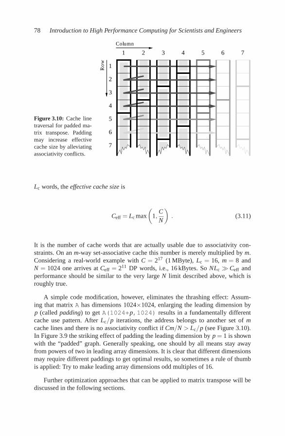
78 Introduction to High Performance Computing for Scientists and Engineers
Figure 3.10: Cache linetraversal for padded ma-trix transpose. Paddingmay increase effectivecache size by alleviatingassociativity conflicts.
Column
Ro
w
1 2 3 4 5 6 7
1
2
3
4
5
6
7
Lc words, the effective cache size is
Ceff = Lc max
(
1,C
N
)
. (3.11)
It is the number of cache words that are actually usable due to associativity con-straints. On an m-way set-associative cache this number is merely multiplied by m.Considering a real-world example with C = 217 (1 MByte), Lc = 16, m = 8 andN = 1024 one arrives at Ceff = 211 DP words, i.e., 16 kBytes. So NLc ≫ Ceff andperformance should be similar to the very large N limit described above, which isroughly true.
A simple code modification, however, eliminates the thrashing effect: Assum-ing that matrix A has dimensions 1024×1024, enlarging the leading dimension byp (called padding) to get A(1024+p,1024) results in a fundamentally differentcache use pattern. After Lc/p iterations, the address belongs to another set of m
cache lines and there is no associativity conflict if Cm/N > Lc/p (see Figure 3.10).In Figure 3.9 the striking effect of padding the leading dimension by p = 1 is shownwith the “padded” graph. Generally speaking, one should by all means stay awayfrom powers of two in leading array dimensions. It is clear that different dimensionsmay require different paddings to get optimal results, so sometimes a rule of thumbis applied: Try to make leading array dimensions odd multiples of 16.
Further optimization approaches that can be applied to matrix transpose will bediscussed in the following sections.

Data access optimization 79
3.5 Algorithm classification and access optimizations
The optimization potential of many loops on cache-based processors can eas-ily be estimated just by looking at basic parameters like the scaling behavior ofdata transfers and arithmetic operations versus problem size. It can then be decidedwhether investing optimization effort would make sense.
3.5.1 O(N)/O(N)
If both the number of arithmetic operations and the number of data transfers(loads/stores) are proportional to the problem size (or “loop length”) N, optimizationpotential is usually very limited. Scalar products, vector additions, and sparse matrix-vector multiplication are examples for this kind of problems. They are inevitablymemory-bound for large N, and compiler-generated code achieves good performancebecause O(N)/O(N) loops tend to be quite simple and the correct software pipeliningstrategy is obvious. Loop nests, however, are a different matter (see below).
But even if loops are not nested there is sometimes room for improvement. As anexample, consider the following vector additions:
1 do i=1,N
2 A(i) = B(i) + C(i)
3 enddo
4 do i=1,N
5 Z(i) = B(i) + E(i)
6 enddo
loop fusion-
! optimized
do i=1,N
A(i) = B(i) + C(i)
! save a load for B(i)
Z(i) = B(i) + E(i)
enddo
Each of the loops on the left has no options left for optimization. The code balanceis 3/1 as there are two loads, one store, and one addition per loop (not counting writeallocates). Array B, however, is loaded again in the second loop, which is unnec-essary: Fusing the loops into one has the effect that each element of B only has tobe loaded once, reducing code balance to 5/2. All else being equal, performance inthe memory-bound case will improve by a factor of 6/5 (if write allocates cannot beavoided, this will be 8/7).
Loop fusion has achieved an O(N) data reuse for the two-loop constellation sothat a complete load stream could be eliminated. In simple cases like the one above,compilers can often apply this optimization by themselves.
3.5.2 O(N2)/O(N2)
In typical two-level loop nests where each loop has a trip count of N, there areO(N2) operations for O(N2) loads and stores. Examples are dense matrix-vector mul-tiply, matrix transpose, matrix addition, etc. Although the situation on the inner levelis similar to the O(N)/O(N) case and the problems are generally memory-bound, thenesting opens new opportunities. Optimization, however, is again usually limited to

80 Introduction to High Performance Computing for Scientists and Engineers
= *+
Figure 3.11: Unoptimized N ×N dense matrix vector multiply. The RHS vector is loaded N
times.
a constant factor of improvement. As an example we consider dense matrix-vectormultiply (MVM):
1 do i=1,N
2 tmp = C(i)
3 do j=1,N
4 tmp = tmp + A(j,i) * B(j)
5 enddo
6 C(i) = tmp
7 enddo
This code has a balance of 1 W/F (two loads for A and B and two flops). Array C
is indexed by the outer loop variable, so updates can go to a register (here clarifiedthrough the use of the scalar tmp although compilers can do this transformationautomatically) and do not count as load or store streams. Matrix A is only loadedonce, but B is loaded N times, once for each outer loop iteration (see Figure 3.11).One would like to apply the same fusion trick as above, but there are not just twobut N inner loops to fuse. The solution is loop unrolling: The outer loop is traversedwith a stride m and the inner loop is replicated m times. We thus have to deal withthe situation that the outer loop count might not be a multiple of m. This case has tobe handled by a remainder loop:
1 ! remainder loop
2 do r=1,mod(N,m)
3 do j=1,N
4 C(r) = C(r) + A(j,r) * B(j)
5 enddo
6 enddo
7 ! main loop
8 do i=r,N,m
9 do j=1,N
10 C(i) = C(i) + A(j,i) * B(j)
11 enddo

Data access optimization 81
12 do j=1,N
13 C(i+1) = C(i+1) + A(j,i+1) * B(j)
14 enddo
15 ! m times
16 ...
17 do j=1,N
18 C(i+m-1) = C(i+m-1) + A(j,i+m-1) * B(j)
19 enddo
20 enddo
The remainder loop is subject to the same optimization techniques as the originalloop, but otherwise unimportant. For this reason we will ignore remainder loops inthe following.
By just unrolling the outer loop we have not gained anything but a considerablecode bloat. However, loop fusion can now be applied easily:
1 ! remainder loop ignored
2 do i=1,N,m
3 do j=1,N
4 C(i) = C(i) + A(j,i) * B(j)
5 C(i+1) = C(i+1) + A(j,i+1) * B(j)
6 ! m times
7 ...
8 C(i+m-1) = C(i+m-1) + A(j,i+m-1) * B(j)
9 enddo
10 enddo
The combination of outer loop unrolling and fusion is often called unroll and jam. Bym-way unroll and jam we have achieved an m-fold reuse of each element of B fromregister so that code balance reduces to (m+1)/2m which is clearly smaller than onefor m > 1. If m is very large, the performance gain can get close to a factor of two. Inthis case array B is only loaded a few times or, ideally, just once from memory. As Ais always loaded exactly once and has size N2, the total memory traffic with m-wayunroll and jam amounts to N2(1+1/m)+N. Figure 3.12 shows the memory accesspattern for two-way unrolled dense matrix-vector multiply.
All this assumes, however, that register pressure is not too large, i.e., the CPUhas enough registers to hold all the required operands used inside the now quitesizeable loop body. If this is not the case, the compiler must spill register data tocache, slowing down the computation (see also Section 2.4.5). Again, compiler logs,if available, can help identify such a situation.
Unroll and jam can be carried out automatically by some compilers at high opti-mization levels. Be aware though that a complex loop body may obscure importantinformation and manual optimization could be necessary, either (as shown above) byhand-coding or compiler directives that specify high-level transformations like un-rolling. Directives, if available, are the preferred alternative as they are much easierto maintain and do not lead to visible code bloat. Regrettably, compiler directives areinherently nonportable.
The matrix transpose code from the previous section is another typical examplefor an O(N2)/O(N2) problem, although in contrast to dense MVM there is no direct

82 Introduction to High Performance Computing for Scientists and Engineers
= *+
Figure 3.12: Two-way unrolled dense matrix vector multiply. The data traffic caused byreloading the RHS vector is reduced by roughly a factor of two. The remainder loop is only asingle (outer) iteration in this example.
opportunity for saving on memory traffic; both matrices have to be read or writtenexactly once. Nevertheless, by using unroll and jam on the “flipped” version a sig-nificant performance boost of nearly 50% is observed (see dotted line in Figure 3.8):
1 do j=1,N,m
2 do i=1,N
3 A(i,j) = B(j,i)
4 A(i,j+1) = B(j+1,i)
5 ...
6 A(i,j+m-1) = B(j+m-1,i)
7 enddo
8 enddo
Naively one would not expect any effect at m = 4 because the basic analysis staysthe same: In the mid-N region the number of available cache lines is large enoughto hold up to Lc columns of the store stream. Figure 3.13 shows the situation form = 2. However, the fact that m words in each of the load stream’s cache lines arenow accessed in direct succession reduces the TLB misses by a factor of m, althoughthe TLB is still way too small to map the whole working set.
Even so, cutting down on TLB misses does not remedy the performance break-down for large N when the cache gets too small to hold N cache lines. It wouldbe nice to have a strategy which reuses the remaining Lc −m words of the stridedstream’s cache lines right away so that each line may be evicted soon and would nothave to be reclaimed later. A “brute force” method is Lc-way unrolling, but this ap-proach leads to large-stride accesses in the store stream and is not a general solutionas large unrolling factors raise register pressure in loops with arithmetic operations.Loop blocking can achieve optimal cache line use without additional register pres-sure. It does not save load or store operations but increases the cache hit ratio. For a

Data access optimization 83
Figure 3.13: Two-way unrolled “flipped” matrix transpose (i.e., with strided load in the origi-nal version).
loop nest of depth d, blocking introduces up to d additional outer loop levels that cutthe original inner loops into chunks:
1 do jj=1,N,b
2 jstart=jj; jend=jj+b-1
3 do ii=1,N,b
4 istart=ii; iend=ii+b-1
5 do j=jstart,jend,m
6 do i=istart,iend
7 a(i,j) = b(j,i)
8 a(i,j+1) = b(j+1,i)
9 ...
10 a(i,j+m-1) = b(j+m-1,i)
11 enddo
12 enddo
13 enddo
14 enddo
In this example we have used two-dimensional blocking with identical blocking fac-tors b for both loops in addition to m-way unroll and jam. This change does not alterthe loop body so the number of registers needed to hold operands stays the same.However, the cache line access characteristics are much improved (see Figure 3.14which shows a combination of two-way unrolling and 4×4 blocking). If the block-ing factors are chosen appropriately, the cache lines of the strided stream will havebeen used completely at the end of a block and can be evicted “soon.” Hence, weexpect the large-N performance breakdown to disappear. The dotted-dashed graphin Figure 3.8 demonstrates that 50×50 blocking combined with four-way unrollingalleviates all memory access problems induced by the strided stream.
Loop blocking is a very general and powerful optimization that can often not beperformed by compilers. The correct blocking factor to use should be determinedexperimentally through careful benchmarking, but one may be guided by typicalcache sizes, i.e., when blocking for L1 cache the aggregated working set size ofall blocked inner loop nests should not be much larger than half the cache. Which

84 Introduction to High Performance Computing for Scientists and Engineers
Figure 3.14: 4×4 blocked and two-way unrolled “flipped” matrix transpose.
cache level to block for depends on the operations performed and there is no generalrecommendation.
3.5.3 O(N3)/O(N2)
If the number of operations is larger than the number of data items by a factorthat grows with problem size, we are in the very fortunate situation to have tremen-dous optimization potential. By the techniques described above (unroll and jam, loopblocking) it is sometimes possible for these kinds of problems to render the imple-mentation cache-bound. Examples for algorithms that show O(N3)/O(N2) charac-teristics are dense matrix-matrix multiplication (MMM) and dense matrix diagonal-ization. It is beyond the scope of this book to develop a well-optimized MMM, letalone eigenvalue calculation, but we can demonstrate the basic principle by meansof a simpler example which is actually of the O(N2)/O(N) type:
1 do i=1,N
2 do j=1,N
3 sum = sum + foo(A(i),B(j))
4 enddo
5 enddo
The complete data set is O(N) here but O(N2) operations (calls to foo(), additions)are performed on it. In the form shown above, array B is loaded from memory N
times, so the total memory traffic amounts to N(N +1) words. m-way unroll and jamis possible and will immediately reduce this to N(N/m + 1), but the disadvantagesof large unroll factors have been pointed out already. Blocking the inner loop with ablocksize of b, however,
1 do jj=1,N,b
2 jstart=jj; jend=jj+b-1
3 do i=1,N
4 do j=jstart,jend
5 sum = sum + foo(A(i),B(j))

Data access optimization 85
6 enddo
7 enddo
8 enddo
has two effects:
• Array B is now loaded only once from memory, provided that b is small enoughso that b elements fit into cache and stay there as long as they are needed.
• Array A is loaded from memory N/b times instead of once.
Although A is streamed through cache N/b times, the probability that the currentblock of B will be evicted is quite low, the reason being that those cache lines areused very frequently and thus kept by the LRU replacement algorithm. This leads toan effective memory traffic of N(N/b+1) words. As b can be made much larger thantypical unrolling factors, blocking is the best optimization strategy here. Unroll andjam can still be applied to enhance in-cache code balance. The basic N2 dependenceis still there, but with a prefactor that can make the difference between memory-bound and cache-bound behavior. A code is cache-bound if main memory bandwidthand latency are not the limiting factors for performance any more. Whether this goalis achievable on a certain architecture depends on the cache size, cache and memoryspeeds, and the algorithm, of course.
Algorithms of the O(N3)/O(N2) type are typical candidates for optimizationsthat can potentially lead to performance numbers close to the theoretical maximum.If blocking and unrolling factors are chosen appropriately, dense matrix-matrix mul-tiply, e.g., is an operation that usually achieves over 90% of peak for N×N matricesif N is not too small. It is provided in highly optimized versions by system vendorsas, e.g., contained in the BLAS (Basic Linear Algebra Subsystem) library. One mightask why unrolling should be applied at all when blocking already achieves the mostimportant task of making the code cache-bound. The reason is that even if all the dataresides in a cache, many processor architectures do not have the capability for sus-taining enough loads and stores per cycle to feed the arithmetic units continuously.For instance, the current x86 processors from Intel can sustain one load and one storeoperation per cycle, which makes unroll and jam mandatory if the kernel of a loopnest uses more than one load stream, especially in cache-bound situations like theblocked O(N2)/O(N) example above.
Although demonstrated here for educational purposes, there is no need to hand-code and optimize standard linear algebra and matrix operations. They should alwaysbe used from optimized libraries, if available. Nevertheless, the techniques describedcan be applied in many real-world codes. An interesting example with some compli-cations is sparse matrix-vector multiply (see Section 3.6).

86 Introduction to High Performance Computing for Scientists and Engineers
+= *
Figure 3.15: Sparse matrix-vector multiply. Dark elements visualize entries involved in up-dating a single LHS element. Unless the sparse matrix rows have no gaps between the first andlast nonzero elements, some indirect addressing of the RHS vector is inevitable.
3.6 Case study: Sparse matrix-vector multiply
An interesting “real-world” application of the blocking and unrolling strategiesdiscussed in the previous sections is the multiplication of a sparse matrix with a vec-tor. It is a key ingredient in most iterative matrix diagonalization algorithms (Lanc-zos, Davidson, Jacobi-Davidson) and usually a performance-limiting factor. A matrixis called sparse if the number of nonzero entries Nnz grows linearly with the num-ber of matrix rows Nr. Of course, only the nonzeros are stored at all for efficiencyreasons. Sparse MVM (sMVM) is hence an O(Nr)/O(Nr) problem and inherentlymemory-bound if Nr is reasonably large. Nevertheless, the presence of loop nestsenables some significant optimization potential. Figure 3.15 shows that sMVM gen-erally requires some strided or even indirect addressing of the RHS vector, althoughthere exist matrices for which memory access patterns are much more favorable. Inthe following we will keep at the general case.
3.6.1 Sparse matrix storage schemes
Several different storage schemes for sparse matrices have been developed, someof which are suitable only for special kinds of matrices [N49]. Of course, memoryaccess patterns and thus performance characteristics of sMVM depend heavily onthe storage scheme used. The two most important and also general formats are CRS(Compressed Row Storage) and JDS (Jagged Diagonals Storage). We will see that

Data access optimization 87
val
col_idx
row_ptr
−4 2 2 8 8 −5 10 −5 10 −6
1 2 1 3 2 4 5 3 3 5
1 83 5 9
−4 2
2 8
8 −5 10
−5
10 −6
1 2 3 4 5
1
2
3
4
5
Figure 3.16: CRS sparse matrix storage format.
CRS is well-suited for cache-based microprocessors while JDS supports dependencyand loop structures that are favorable on vector systems.
In CRS, an array val of length Nnz is used to store all nonzeros of the matrix,row by row, without any gaps, so some information about which element of valoriginally belonged to which row and column must be supplied. This is done bytwo additional integer arrays, col_idx of length Nnz and row_ptr of length Nr.col_idx stores the column index of each nonzero in val. row_ptr contains theindices at which new rows start in val (see Figure 3.16). The basic code to performan MVM using this format is quite simple:
1 do i = 1,Nr2 do j = row_ptr(i), row_ptr(i+1) - 1
3 C(i) = C(i) + val(j) * B(col_idx(j))
4 enddo
5 enddo
The following points should be noted:
• There is a long outer loop (length Nr).
• The inner loop may be “short” compared to typical microprocessor pipelinelengths.
• Access to result vector C is well optimized: It is only loaded once from mainmemory.
• The nonzeros in val are accessed with stride one.
• As expected, the RHS vector B is accessed indirectly. This may, however, notbe a serious performance problem depending on the exact structure of the ma-trix. If the nonzeros are concentrated mainly around the diagonal, there willeven be considerable spatial and/or temporal locality.
• Bc = 5/4 W/F if the integer load to col_idx is counted with four bytes. Weare neglecting the possibly much larger transfer volume due to partially usedcache lines.
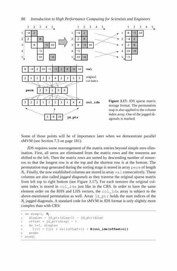
88 Introduction to High Performance Computing for Scientists and Engineers
val
col_idx
jd_ptr
perm
original
col index
−4 2
82
8 −5 10
−5
10 −6
10
−5
10
2
8
−5
−6
8
2
−4 8
−4
2
10
−5
−6
8
2
−5 10
8 −4 2 10 −5 −5 2 8 −6 10
2 1 1 3 3 4 2 3 5 5
45132
3 22 1 1 5 3 1 4 4
1 106
5
4
3
2
1
1 2 3 4
1
2
3
4
5
1 2 3 4 5 1 2 3 4
1
2
3
4
5
55
Figure 3.17: JDS sparse matrixstorage format. The permutationmap is also applied to the columnindex array. One of the jagged di-agonals is marked.
Some of those points will be of importance later when we demonstrate parallelsMVM (see Section 7.3 on page 181).
JDS requires some rearrangement of the matrix entries beyond simple zero elim-ination. First, all zeros are eliminated from the matrix rows and the nonzeros areshifted to the left. Then the matrix rows are sorted by descending number of nonze-ros so that the longest row is at the top and the shortest row is at the bottom. Thepermutation map generated during the sorting stage is stored in array perm of lengthNr. Finally, the now established columns are stored in array val consecutively. Thesecolumns are also called jagged diagonals as they traverse the original sparse matrixfrom left top to right bottom (see Figure 3.17). For each nonzero the original col-umn index is stored in col_idx just like in the CRS. In order to have the sameelement order on the RHS and LHS vectors, the col_idx array is subject to theabove-mentioned permutation as well. Array jd_ptr holds the start indices of theNj jagged diagonals. A standard code for sMVM in JDS format is only slightly morecomplex than with CRS:
1 do diag=1, Nj2 diagLen = jd_ptr(diag+1) - jd_ptr(diag)
3 offset = jd_ptr(diag) - 1
4 do i=1, diagLen
5 C(i) = C(i) + val(offset+i) * B(col_idx(offset+i))
6 enddo
7 enddo
Data access optimization 89
The perm array storing the permutation map is not required here; usually, all sMVMoperations are done in permuted space. These are the notable properties of this loop:
• There is a long inner loop without dependencies, which makes JDS a muchbetter storage format for vector processors than CRS.
• The outer loop is short (number of jagged diagonals).
• The result vector is loaded multiple times (at least partially) from memory, sothere might be some optimization potential.
• The nonzeros in val are accessed with stride one.
• The RHS vector is accessed indirectly, just as with CRS. The same commentsas above do apply, although a favorable matrix layout would feature straightdiagonals, not compact rows. As an additional complication the matrix rowsas well as the RHS vector are permuted.
• Bc = 9/4 W/F if the integer load to col_idx is counted with four bytes.
The code balance numbers of CRS and JDS sMVM seem to be quite in favor of CRS.
3.6.2 Optimizing JDS sparse MVM
Unroll and jam should be applied to the JDS sMVM, but it usually requires thelength of the inner loop to be independent of the outer loop index. Unfortunately, thejagged diagonals are generally not all of the same length, violating this condition.However, an optimization technique called loop peeling can be employed which, form-way unrolling, cuts rectangular m× x chunks and leaves m− 1 partial diagonalsover for separate treatment (see Figure 3.18; the remainder loop is omitted as usual):
1 do diag=1,Nj,2 ! two-way unroll & jam
2 diagLen = min( (jd_ptr(diag+1)-jd_ptr(diag)) ,\
3 (jd_ptr(diag+2)-jd_ptr(diag+1)) )
4 offset1 = jd_ptr(diag) - 1
5 offset2 = jd_ptr(diag+1) - 1
6 do i=1, diagLen
7 C(i) = C(i)+val(offset1+i)*B(col_idx(offset1+i))
8 C(i) = C(i)+val(offset2+i)*B(col_idx(offset2+i))
9 enddo
10 ! peeled-off iterations
11 offset1 = jd_ptr(diag)
12 do i=(diagLen+1),(jd_ptr(diag+1)-jd_ptr(diag))
13 c(i) = c(i)+val(offset1+i)*b(col_idx(offset1+i))
14 enddo
15 enddo
Assuming that the peeled-off iterations account for a negligible contribution to CPUtime, m-way unroll and jam reduces code balance to
Bc =
(
1m
+54
)
W/F .

90 Introduction to High Performance Computing for Scientists and Engineers
Figure 3.18: JDS matrix traversal withtwo-way unroll and jam and loop peeling.The peeled iterations are marked.
Figure 3.19: JDS matrix traversal withfour-way loop blocking.
If m is large enough, this can get close to the CRS balance. However, as explained be-fore large m leads to strong register pressure and is not always desirable. Generally, asensible combination of unrolling and blocking is employed to reduce memory traf-fic and enhance in-cache performance at the same time. Blocking is indeed possiblefor JDS sMVM as well (see Figure 3.19):
1 ! loop over blocks
2 do ib=1, Nr, b
3 block_start = ib
4 block_end = min(ib+b-1, Nr)
5 ! loop over diagonals in one block
6 do diag=1, Nj7 diagLen = jd_ptr(diag+1)-jd_ptr(diag)
8 offset = jd_ptr(diag) - 1
9 if(diagLen .ge. block_start) then
10 ! standard JDS sMVM kernel
11 do i=block_start, min(block_end,diagLen)
12 B(i) = B(i)+val(offset+i)*B(col_idx(offset+i))
13 enddo
14 endif
15 enddo
16 enddo
With this optimization the result vector is effectively loaded only once from memoryif the block size b is not too large. The code should thus get similar performance asthe CRS version, although code balance has not been changed. As anticipated abovewith dense matrix transpose, blocking does not optimize for register reuse but forcache utilization.

Data access optimization 91
CRS JDSvanilla
JDSunroll=2
JDSblock=400
0
100
200
300
400
MF
lops/s
ec
AMD Opteron
Intel Itanium2 (SGI Altix)
Intel Xeon/Core
Figure 3.20: Performance comparison of sparse MVM codes with different optimizations. Amatrix with 1.7× 10⁷ unknowns and 20 jagged diagonals was chosen. The blocking size of400 has proven to be optimal for a wide range of architectures.
Figure 3.20 shows a performance comparison of CRS and plain, two-way un-rolled and blocked (b = 400) JDS sMVM on three different architectures, for a testmatrix from solid state physics (six-site one-dimensional Holstein-Hubbard modelat half filling). The CRS variant seems to be preferable for standard AMD and Intelmicroprocessors, which is not surprising because it features the lowest code balanceright away without any subsequent manual optimizations and the short inner looplength is less unfavorable on CPUs with out-of-order capabilities. The Intel Itanium2processor with its EPIC architecture [V113], however, shows mediocre performancefor CRS and tops at the blocked JDS version. This architecture cannot cope very wellwith the short loops of CRS due to the absence of out-of-order processing and thecompiler, despite detecting all instruction-level parallelism on the inner loop level,not being able to overlap the wind-down of one row with the wind-up phase of thenext. This effect would certainly be much more pronounced if the working set did fitinto the cache [O56].
Problems
For solutions see page 289 ff.
3.1 Strided access. How do the balance and lightspeed considerations in Sec-
92 Introduction to High Performance Computing for Scientists and Engineers
tion 3.1 have to be modified if one or more arrays are accessed with nonunitstride? What kind of performance characteristic do you expect for a stride-svector triad,
1 do i=1,N,s
2 A(i) = B(i) + C(i) * D(i)
3 enddo
with respect to s if N is large?
3.2 Balance fun. Calculate code balance for the following loop kernels, assumingthat all arrays have to be loaded from memory and ignoring the latency prob-lem (appropriate loops over the counter variables i and j are always implied):
(a) Y(j) = Y(j) + A(i,j) * B(i) (matrix-vector multiply)
(b) s = s + A(i) * A(i) (vector norm)
(c) s = s + A(i) * B(i) (scalar product)
(d) s = s + A(i) * B(K(i)) (scalar product with indirect access)
All arrays are of DP floating-point type except K which stores 4-byte integers.s is a double precision scalar. Calculate expected application performancebased on theoretical peak bandwidth and STREAM bandwidths in MFlops/secfor those kernels on one core of a Xeon 5160 processor and on the prototypicalvector processor described in Section 1.6. The Xeon CPU has a cache line sizeof 64 bytes. You may assume that N is large so that the arrays do not fit intoany cache. For case (d), give numbers for best and worst case scenarios on theXeon.
3.3 Performance projection. In future mainstream microarchitectures, SIMD ca-pabilities will be greatly enhanced. One of the possible new features is thatx86 processors will be capable of executing MULT and ADD instructions on256-bit (instead of 128-bit) registers, i.e., four DP floating-point values, con-currently. This will effectively double the peak performance per cycle from 4to 8 flops, given that the L1 cache bandwidth is improved by the same fac-tor. Assuming that other parameters like memory bandwidth and clock speedstay the same, estimate the expected performance gain for using this feature,compared to a single current Intel “Core i7” core (effective STREAM-basedmachine balance of 0.12 W/F). Assume a perfectly SIMD-vectorized applica-tion that today spends 60% of its compute time on code that has a balanceof 0.04 W/F and the remaining 40% in code with a balance of 0.5 W/F. If themanufacturers chose to extend SIMD capabilities even more, e.g., by intro-ducing very large vector lengths, what is the absolute limit for the expectedperformance gain in this situation?
3.4 Optimizing 3D Jacobi. Generalize the 2D Jacobi algorithm introduced in Sec-tion 3.3 to three dimensions. Do you expect a change in performance char-

Data access optimization 93
acteristics with varying inner loop length (Figure 3.6)? Considering the opti-mizations for dense matrix transpose (Section 3.4), can you think of a way toeliminate some of the performance breakdowns?
3.5 Inner loop unrolling revisited. Up to now we have encountered the possibilityof unrolling inner loops only in the contexts of software pipelining and SIMDoptimizations (see Chapter 2). Can inner loop unrolling also improve code bal-ance in some situations? What are the prospects for improving the performanceof a Jacobi solver by unrolling the inner loop?
3.6 Not unrollable? Consider the multiplication of a lower triangular matrix witha vector:
1 do r=1,N
2 do c=1,r
3 y(r) = y(r) + a(c,r) * x(c)
4 enddo
5 enddo
Can you apply “unroll and jam” to the outer loop here (see Section 3.5.2 onpage 81) to reduce code balance? Write a four-way unrolled version of abovecode. No special assumptions about Nmay be made (other than being positive),and no matrix elements of Amay be accessed that are outside the lower triangle(including the diagonal).
3.7 Application optimization. Which optimization strategies would you suggest forthe piece of code below? Write down a transformed version of the code whichyou expect to give the best performance.
1 double precision, dimension(N,N) :: mat,s
2 double precision :: val
3 integer :: i,j
4 integer, dimension(N) :: v
5 ! ... v and s may be assumed to hold valid data
6 do i=1,N
7 do j=1,N
8 val = DBLE(MOD(v(i),256))
9 mat(i,j) = s(i,j)*(SIN(val)*SIN(val)-COS(val)*COS(val))
10 enddo
11 enddo
No assumptions about the size of N may be made. You may, however, assumethat the code is part of a subroutine which gets called very frequently. s and vmay change between calls, and all elements of v are positive.
3.8 TLB impact. The translation lookaside buffer (TLB) of even the most modernprocessors is scarcely large enough to even store the mappings of all memorypages that reside in the outer-level data cache. Why are TLBs so small? Isn’tthis a performance bottleneck by design? What are the benefits of larger pages?


Chapter 4
Parallel computers
We speak of parallel computing whenever a number of “compute elements” (cores)solve a problem in a cooperative way. All modern supercomputer architectures de-pend heavily on parallelism, and the number of CPUs in large-scale supercomputersincreases steadily. A common measure for supercomputer “speed” has been estab-lished by the Top500 list [W121], which is published twice a year and ranks paral-lel computers based on their performance in the LINPACK benchmark. LINPACKsolves a dense system of linear equations of unspecified size. It is not generally ac-cepted as a good metric because it covers only a single architectural aspect (peakperformance). Although other, more realistic alternatives like the HPC Challengebenchmarks [W122] have been proposed, the simplicity of LINPACK and its ease ofuse through efficient open-source implementations have preserved its dominance inthe Top500 ranking for nearly two decades now. Nevertheless, the list can still serve
5-8
9-1
6
17-3
2
33-6
4
65-1
28
129-2
56
257-5
12
513-1
k
1k-
2k
2k-
4k
4k-
8k
8k-
16k
16k-
32k
32k-
64k
64k-
128k
128k-
256k
3-4
Number of cores per system
0
50
100
150
200
250
300
Nu
mb
er
of
syste
ms
November 1999
November 2004
November 2009
Figure 4.1: Number of systems versus core count in the November 1999, 2004, and 2009Top500 lists. The average number of CPUs has grown 50-fold in ten years. Between 2004 and2009, the advent of multicore chips resulted in a dramatic boost in typical core counts. Datataken from [W121].
95

96 Introduction to High Performance Computing for Scientists and Engineers
as an important indicator for trends in supercomputing. The main tendency is clearlyvisible from a comparison of processor number distributions in Top500 systems (seeFigure 4.1): Top of the line HPC systems do not rely on Moore’s Law alone for per-formance but parallelism becomes more important every year. This trend has beenaccelerating recently by the advent of multicore processors — apart from the occa-sional parallel vector computer, the latest lists contain no single-core systems anymore (see also Section 1.4). We can certainly provide no complete overview on cur-rent parallel computer technology, but recommend the regularly updated Overview
of recent supercomputers by van der Steen and Dongarra [W123].In this chapter we will give an introduction to the fundamental variants of par-
allel computers: the shared-memory and the distributed-memory type. Both utilizenetworks for communication between processors or, more generally, “computing el-ements,” so we will outline the basic design rules and performance characteristics forthe common types of networks as well.
4.1 Taxonomy of parallel computing paradigms
A widely used taxonomy for describing the amount of concurrent control anddata streams present in a parallel architecture was proposed by Flynn [R38]. Thedominating concepts today are the SIMD and MIMD variants:
SIMD Single Instruction, Multiple Data. A single instruction stream, either on asingle processor (core) or on multiple compute elements, provides parallelismby operating on multiple data streams concurrently. Examples are vector pro-cessors (see Section 1.6), the SIMD capabilities of modern superscalar micro-processors (see Section 2.3.3), and Graphics Processing Units (GPUs). Histor-ically, the all but extinct large-scale multiprocessor SIMD parallelism was im-plemented in Thinking Machines’ Connection Machine supercomputer [R36].
MIMD Multiple Instruction, Multiple Data. Multiple instruction streams on multi-ple processors (cores) operate on different data items concurrently. The shared-memory and distributed-memory parallel computers described in this chapterare typical examples for the MIMD paradigm.
There are actually two more categories, called SISD (Single Instruction Single Data)and MISD (Multiple Instruction Single Data), the former describing conventional,nonparallel, single-processor execution following the original pattern of the stored-program digital computer (see Section 1.1), while the latter is not regarded as a usefulparadigm in practice.
Strictly processor-based instruction-level parallelism as employed in superscalar,pipelined execution (see Sections 1.2.3 and 1.2.4) is not included in this categoriza-tion, although one may argue that it could count as MIMD. However, in what followswe will restrict ourselves to the multiprocessor MIMD parallelism built into shared-and distributed-memory parallel computers.

Parallel computers 97
4.2 Shared-memory computers
A shared-memory parallel computer is a system in which a number of CPUswork on a common, shared physical address space. Although transparent to theprogrammer as far as functionality is concerned, there are two varieties of shared-memory systems that have very different performance characteristics in terms ofmain memory access:
• Uniform Memory Access (UMA) systems exhibit a “flat” memory model: La-tency and bandwidth are the same for all processors and all memory locations.This is also called symmetric multiprocessing (SMP). At the time of writing,single multicore processor chips (see Section 1.4) are “UMA machines.” How-ever, “cluster on a chip” designs that assign separate memory controllers todifferent groups of cores on a die are already beginning to appear.
• On cache-coherent Nonuniform Memory Access (ccNUMA) machines, mem-ory is physically distributed but logically shared. The physical layout of suchsystems is quite similar to the distributed-memory case (see Section 4.3), butnetwork logic makes the aggregated memory of the whole system appear asone single address space. Due to the distributed nature, memory access per-formance varies depending on which CPU accesses which parts of memory(“local” vs. “remote” access).
With multiple CPUs, copies of the same cache line may reside in different caches,probably in modified state. So for both above varieties, cache coherence protocols
must guarantee consistency between cached data and data in memory at all times.Details about UMA, ccNUMA, and cache coherence mechanisms are provided in thefollowing sections. The dominating shared-memory programming model in scientificcomputing, OpenMP, will be introduced in Chapter 6.
4.2.1 Cache coherence
Cache coherence mechanisms are required in all cache-based multiprocessor sys-tems, whether they are of the UMA or the ccNUMA kind. This is because copies ofthe same cache line could potentially reside in several CPU caches. If, e.g., one ofthose gets modified and evicted to memory, the other caches’ contents reflect out-dated data. Cache coherence protocols ensure a consistent view of memory under allcircumstances.
Figure 4.2 shows an example on two processors P1 and P2 with respective cachesC1 and C2. Each cache line holds two items. Two neighboring items A1 and A2 inmemory belong to the same cache line and are modified by P1 and P2, respectively.Without cache coherence, each cache would read the line from memory, A1 wouldget modified in C1, A2 would get modified in C2 and some time later both modifiedcopies of the cache line would have to be evicted. As all memory traffic is handled in

98 Introduction to High Performance Computing for Scientists and Engineers
��������������������
����������������
C1 C2
MemoryA1 A2
A1 A2 A1 A2
P1 P2
1 5
3 7
2 4 6
1. C1 requests exclusive CL ownership
2. set CL in C2 to state I
3. CL has state E in C1 → modify A1 in C1and set to state M
4. C2 requests exclusive CL ownership
5. evict CL from C1 and set to state I
6. load CL to C2 and set to state E
7. modify A2 in C2 and set to state M in C2
Figure 4.2: Two processors P1, P2 modify the two parts A1, A2 of the same cache line incaches C1 and C2. The MESI coherence protocol ensures consistency between cache andmemory.
chunks of cache line size, there is no way to determine the correct values of A1 andA2 in memory.
Under control of cache coherence logic this discrepancy can be avoided. As anexample we pick the MESI protocol, which draws its name from the four possiblestates a cache line can assume:
M modified: The cache line has been modified in this cache, and it resides in noother cache than this one. Only upon eviction will memory reflect the mostcurrent state.
E exclusive: The cache line has been read from memory but not (yet) modified.However, it resides in no other cache.
S shared: The cache line has been read from memory but not (yet) modified. Theremay be other copies in other caches of the machine.
I invalid: The cache line does not reflect any sensible data. Under normal circum-stances this happens if the cache line was in the shared state and another pro-cessor has requested exclusive ownership.
The order of events is depicted in Figure 4.2. The question arises how a cache line instate M is notified when it should be evicted because another cache needs to read themost current data. Similarly, cache lines in state S or E must be invalidated if anothercache requests exclusive ownership. In small systems a bus snoop is used to achievethis: Whenever notification of other caches seems in order, the originating cachebroadcasts the corresponding cache line address through the system, and all caches“snoop” the bus and react accordingly. While simple to implement, this method hasthe crucial drawback that address broadcasts pollute the system buses and reduceavailable bandwidth for “useful” memory accesses. A separate network for coherencetraffic can alleviate this effect but is not always practicable.
A better alternative, usually applied in larger ccNUMA machines, is a directory-
based protocol where bus logic like chipsets or memory interfaces keep track of the
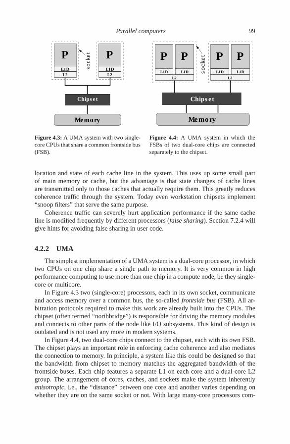
Parallel computers 99
so
cke
tP P
Chipset
Memory
L1D
L2
L1D
L2
Figure 4.3: A UMA system with two single-core CPUs that share a common frontside bus(FSB).
P
so
cke
t P
Chipset
Memory
L1D
L2 L2
L1D
P PL1D L1D
Figure 4.4: A UMA system in which theFSBs of two dual-core chips are connectedseparately to the chipset.
location and state of each cache line in the system. This uses up some small partof main memory or cache, but the advantage is that state changes of cache linesare transmitted only to those caches that actually require them. This greatly reducescoherence traffic through the system. Today even workstation chipsets implement“snoop filters” that serve the same purpose.
Coherence traffic can severely hurt application performance if the same cacheline is modified frequently by different processors (false sharing). Section 7.2.4 willgive hints for avoiding false sharing in user code.
4.2.2 UMA
The simplest implementation of a UMA system is a dual-core processor, in whichtwo CPUs on one chip share a single path to memory. It is very common in highperformance computing to use more than one chip in a compute node, be they single-core or multicore.
In Figure 4.3 two (single-core) processors, each in its own socket, communicateand access memory over a common bus, the so-called frontside bus (FSB). All ar-bitration protocols required to make this work are already built into the CPUs. Thechipset (often termed “northbridge”) is responsible for driving the memory modulesand connects to other parts of the node like I/O subsystems. This kind of design isoutdated and is not used any more in modern systems.
In Figure 4.4, two dual-core chips connect to the chipset, each with its own FSB.The chipset plays an important role in enforcing cache coherence and also mediatesthe connection to memory. In principle, a system like this could be designed so thatthe bandwidth from chipset to memory matches the aggregated bandwidth of thefrontside buses. Each chip features a separate L1 on each core and a dual-core L2group. The arrangement of cores, caches, and sockets make the system inherentlyanisotropic, i.e., the “distance” between one core and another varies depending onwhether they are on the same socket or not. With large many-core processors com-

100 Introduction to High Performance Computing for Scientists and Engineers
Figure 4.5: AccNUMA systemwith two localitydomains (one persocket) and eightcores.
coherent
link
PL1D
L2
PL1D
L2
PL1D
L2
PL1D
L2
Memory Interface
L3
MemoryMemory
PL1D
L2
PL1D
L2
PL1D
L2
PL1D
L2
Memory Interface
L3
prising multilevel cache groups, the situation gets more complex still. See Section 1.4for more information about shared caches and the consequences of anisotropy.
The general problem of UMA systems is that bandwidth bottlenecks are boundto occur when the number of sockets (or FSBs) is larger than a certain limit. In verysimple designs like the one in Figure 4.3, a common memory bus is used that canonly transfer data to one CPU at a time (this is also the case for all multicore chipsavailable today but may change in the future).
In order to maintain scalability of memory bandwidth with CPU number, non-blocking crossbar switches can be built that establish point-to-point connections be-tween sockets and memory modules, similar to the chipset in Figure 4.4. Due to thevery large aggregated bandwidths those become very expensive for a larger numberof sockets. At the time of writing, the largest UMA systems with scalable bandwidth(the NEC SX-9 vector nodes) have sixteen sockets. This problem can only be solvedby giving up the UMA principle.
4.2.3 ccNUMA
In ccNUMA, a locality domain (LD) is a set of processor cores together withlocally connected memory. This memory can be accessed in the most efficient way,i.e., without resorting to a network of any kind. Multiple LDs are linked via a coher-
ent interconnect, which allows transparent access from any processor to any otherprocessor’s memory. In this sense, a locality domain can be seen as a UMA “build-ing block.” The whole system is still of the shared-memory kind, and runs a singleOS instance. Although the ccNUMA principle provides scalable bandwidth for verylarge processor counts, it is also found in inexpensive small two- or four-socket nodesfrequently used for HPC clustering (see Figure 4.5). In this particular example twolocality domains, i.e., quad-core chips with separate caches and a common interfaceto local memory, are linked using a high-speed connection. HyperTransport (HT)and QuickPath (QPI) are the current technologies favored by AMD and Intel, respec-tively, but other solutions do exist. Apart from the minor peculiarity that the socketscan drive memory directly, making separate interface chips obsolete, the intersocketlink can mediate direct, cache-coherent memory accesses. From the programmer’spoint of view this mechanism is transparent: All the required protocols are handledby hardware.
Figure 4.6 shows another approach to ccNUMA that is flexible enough to scale

Parallel computers 101
NL
P P P P P P P PL1D
L2
L3 L3
L2
L1D L1D
L2
L3 L3
L2
L1D L1D
L2
L3 L3
L2
L1D L1D
L2
L3 L3
L2
L1D
Memory Memory Memory Memory
R
R
S S
S S
Figure 4.6: A ccNUMAsystem (SGI Altix) withfour locality domains,each comprising onesocket with two cores.The LDs are connectedvia a routed NUMALink(NL) network usingrouters (R).
to large machines. It is used in Intel-based SGI Altix systems with up to thousandsof cores in a single address space and a single OS instance. Each processor socket isconnected to a communication interface (S), which provides memory access as wellas connectivity to the proprietary NUMALink (NL) network. The NL network relieson routers (R) to switch connections for nonlocal access. As with HyperTransportand QuickPath, the NL hardware allows for transparent access to the whole addressspace of the machine from all cores. Although shown here only with four sockets,multilevel router fabrics can be built that scale up to hundreds of CPUs. It must,however, be noted that each piece of hardware inserted into a data connection (com-munication interfaces, routers) adds to latency, making access characteristics veryinhomogeneous across the system. Furthermore, providing wire-equivalent speedand nonblocking bandwidth for remote memory access in large systems is extremelyexpensive. For these reasons, large supercomputers and cost-effective smaller clus-ters are always made from shared-memory building blocks (usually of the ccNUMAtype) that are connected via some network without ccNUMA capabilities. See Sec-tions 4.3 and 4.4 for details.
In all ccNUMA designs, network connections must have bandwidth and latencycharacteristics that are at least the same order of magnitude as for local memory.Although this is the case for all contemporary systems, even a penalty factor of twofor nonlocal transfers can badly hurt application performance if access cannot be re-stricted inside locality domains. This locality problem is the first of two obstaclesto take with high performance software on ccNUMA. It occurs even if there is onlyone serial program running on a ccNUMA machine. The second problem is poten-tial contention if two processors from different locality domains access memory inthe same locality domain, fighting for memory bandwidth. Even if the network isnonblocking and its performance matches the bandwidth and latency of local access,contention can occur. Both problems can be solved by carefully observing the dataaccess patterns of an application and restricting data access of each processor to itsown locality domain. Chapter 8 will elaborate on this topic.
In inexpensive ccNUMA systems I/O interfaces are often connected to a sin-gle LD. Although I/O transfers are usually slow compared to memory bandwidth,there are, e.g., high-speed network interconnects that feature multi-GB bandwidths

102 Introduction to High Performance Computing for Scientists and Engineers
Figure 4.7: Simplifiedprogrammer’s view, or“programming model,”of a distributed-memoryparallel computer: Se-parate processes run onprocessors (P), commu-nicating via interfaces(NI) over some network.No process can accessanother process’ memo-ry (M) directly, althoughprocessors may reside inshared memory.
NI NI NI NI NI
CCCCC
M M M M
Communication network
M
P P P P P
between compute nodes. If data arrives at the “wrong” locality domain, written byan I/O driver that has positioned its buffer space disregarding any ccNUMA con-straints, it should be copied to its optimal destination, reducing effective bandwidthby a factor of four (three if write allocates can be avoided, see Section 1.3.1). In thiscase even the most expensive interconnect hardware is wasted. In truly scalable cc-NUMA designs this problem is circumvented by distributing I/O connections acrossthe whole machine and using ccNUMA-aware drivers.
4.3 Distributed-memory computers
Figure 4.7 shows a simplified block diagram of a distributed-memory parallelcomputer. Each processor P is connected to exclusive local memory, i.e., no otherCPU has direct access to it. Nowadays there are actually no distributed-memorysystems any more that implement such a layout. In this respect, the sketch is tobe seen as a programming model only. For price/performance reasons all parallelmachines today, first and foremost the popular PC clusters, consist of a number ofshared-memory “compute nodes” with two or more CPUs (see the next section);the “distributed-memory programmer’s” view does not reflect that. It is even pos-sible (and quite common) to use distributed-memory programming on pure shared-memory machines.
Each node comprises at least one network interface (NI) that mediates the con-nection to a communication network. A serial process runs on each CPU that cancommunicate with other processes on other CPUs by means of the network. It iseasy to envision how several processors could work together on a common problemin a shared-memory parallel computer, but as there is no remote memory access ondistributed-memory machines, the problem has to be solved cooperatively by sendingmessages back and forth between processes. Chapter 9 gives an introduction to thedominating message passing standard, MPI. Although message passing is much more

Parallel computers 103
Network Int. Network Int. Network Int. Network Int.
Communication network
P P
Memory
P P
Memory
P P
Memory
P P
Memory
P P
Memory
P P
Memory
P P
Memory
P P
Memory
Figure 4.8: Typical hybrid system with shared-memory nodes (ccNUMA type). Two-socketbuilding blocks represent the price vs. performance “sweet spot” and are thus found in manycommodity clusters.
complex to use than any shared-memory programming paradigm, large-scale super-computers are exclusively of the distributed-memory variant on a “global” level.
The distributed-memory architecture outlined here is also named No Remote
Memory Access (NORMA). Some vendors provide libraries and sometimes hardwaresupport for limited remote memory access functionality even on distributed-memorymachines. Since such features are strongly vendor-specific, and there is no widelyaccepted standard available, a detailed coverage would be beyond the scope of thisbook.
There are many options for the choice of interconnect. In the simplest case onecould use standard switched Ethernet, but a number of more advanced technologieshave emerged that can easily have ten times the performance of Gigabit Ethernet(see Section 4.5.1 for an account of basic performance characteristics of networks).As will be shown in Section 5.3, the layout and “speed” of the network has consid-erable impact on application performance. The most favorable design consists of anonblocking “wirespeed” network that can switch N/2 connections between its N
participants without any bottlenecks. Although readily available for small systemswith tens to a few hundred nodes, nonblocking switch fabrics become vastly expen-sive on very large installations and some compromises are usually made, i.e., therewill be a bottleneck if all nodes want to communicate concurrently. See Section 4.5for details on network topologies.
4.4 Hierarchical (hybrid) systems
As already mentioned, large-scale parallel computers are neither of the purelyshared-memory nor of the purely distributed-memory type but a mixture of both, i.e.,there are shared-memory building blocks connected via a fast network. This makesthe overall system design even more anisotropic than with multicore processors and

104 Introduction to High Performance Computing for Scientists and Engineers
ccNUMA nodes, because the network adds another level of communication char-acteristics (see Figure 4.8). The concept has clear advantages in terms of price vs.performance; it is cheaper to build a shared-memory node with two sockets insteadof two nodes with one socket each, as much of the infrastructure can be shared.Moreover, with more cores or sockets sharing a single network connection, the costfor networking is reduced.
Two-socket building blocks are currently the “sweet spot” for inexpensive com-
modity clusters, i.e., systems built from standard components that were not specif-ically designed for high performance computing. Depending on which applicationsare run on the system, this compromise may lead to performance limitations due tothe reduced available network bandwidth per core. Moreover, it is per se unclear howthe complex hierarchy of cores, cache groups, sockets and nodes can be utilized effi-ciently. The only general consensus is that the optimal programming model is highlyapplication- and system-dependent. Options for programming hierarchical systemsare outlined in Chapter 11.
Parallel computers with hierarchical structures as described above are also calledhybrids. The concept is actually more generic and can also be used to categorizeany system with a mixture of available programming paradigms on different hard-ware layers. Prominent examples are clusters built from nodes that contain, be-sides the “usual” multicore processors, additional accelerator hardware, rangingfrom application-specific add-on cards to GPUs (graphics processing units), FPGAs(field-programmable gate arrays), ASICs (application specific integrated circuits),co-processors, etc.
4.5 Networks
We will see in Section 5.3.6 that communication overhead can have significantimpact on application performance. The characteristics of the network that connectsthe “execution units,” “processors,” “compute nodes,” or whatever play a dominantrole here. A large variety of network technologies and topologies are available onthe market, some proprietary and some open. This section tries to shed some lighton the topologies and performance aspects of the different types of networks usedin high performance computing. We try to keep the discussion independent of con-crete implementations or programming models, and most considerations apply todistributed-memory, shared-memory, and hierarchical systems alike.
4.5.1 Basic performance characteristics of networks
As mentioned before, there are various options for the choice of a network ina parallel computer. The simplest and cheapest solution to date is Gigabit Ethernet,which will suffice for many throughput applications but is far too slow for parallelprograms with any need for fast communication. At the time of writing, the domi-

Parallel computers 105
time
Process 0 Process 1
����������������������������������������������������������������
����������������������������������������������������������������
Receive
message
Receive
message
Sendmessage
Sendmessage
Figure 4.9: Timeline for a “Ping-Pong” data exchange betweentwo processes. PingPong reportsthe time it takes for a message oflength N bytes to travel from pro-cess 0 to process 1 and back.
nating distributed-memory interconnect, especially in commodity clusters, is Infini-
Band.
Point-to-point connections
Whatever the underlying hardware may be, the communication characteristicsof a single point-to-point connection can usually be described by a simple model:Assuming that the total transfer time for a message of size N [bytes] is composed oflatency and streaming parts,
T = Tℓ +N
B(4.1)
and B being the maximum (asymptotic) network bandwidth in MBytes/sec, the ef-fective bandwidth is
Beff =N
Tℓ + NB
. (4.2)
Note that in the most general case Tℓ and B depend on the message length N. Amulticore processor chip with a shared cache as shown, e.g., in Figure 1.18, is atypical example: Latency and bandwidth of message transfers between two cores onthe same socket certainly depend on whether the message fits into the shared cache.We will ignore such effects for now, but they are vital to understand the finer detailsof message passing optimizations, which will be covered in Chapter 10.
For the measurement of latency and effective bandwidth the PingPong bench-mark is frequently used. The code sends a message of size N [bytes] once back andforth between two processes running on different processors (and probably differentnodes as well; see Figure 4.9). In pseudocode this looks as follows:
1 myID = get_process_ID()
2 if(myID.eq.0) then
3 targetID = 1
4 S = get_walltime()
5 call Send_message(buffer,N,targetID)
6 call Receive_message(buffer,N,targetID)
7 E = get_walltime()
8 MBYTES = 2*N/(E-S)/1.d6 ! MBytes/sec rate

106 Introduction to High Performance Computing for Scientists and Engineers
9 TIME = (E-S)/2*1.d6 ! transfer time in microsecs
10 ! for single message
11 else
12 targetID = 0
13 call Receive_message(buffer,N,targetID)
14 call Send_message(buffer,N,targetID)
15 endif
Bandwidth in MBytes/sec is then reported for different N. In reality one would use anappropriate messaging library like the Message Passing Interface (MPI), which willbe introduced in Chapter 9. The data shown below was obtained using the standard“Intel MPI Benchmarks” (IMB) suite [W124].
In Figure 4.10, the model parameters in (4.2) are fitted to real data measured ona Gigabit Ethernet network. This simple model is able to describe the gross featureswell: We observe very low bandwidth for small message sizes, because latency dom-inates the transfer time. For very large messages, latency plays no role any more andeffective bandwidth saturates. The fit parameters indicate plausible values for GigabitEthernet; however, latency can certainly be measured directly by taking the N = 0limit of transfer time (inset in Figure 4.10). Obviously, the fit cannot reproduce Tℓ
accurately. See below for details.In contrast to bandwidth limitations, which are usually set by the physical param-
eters of data links, latency is often composed of several contributions:
• All data transmission protocols have some overhead in the form of administra-tive data like message headers, etc.
• Some protocols (like, e.g., TCP/IP as used over Ethernet) define minimummessage sizes, so even if the application sends a single byte, a small “frame”of N > 1 bytes is transmitted.
• Initiating a message transfer is a complicated process that involves multiplesoftware layers, depending on the complexity of the protocol. Each softwarelayer adds to latency.
• Standard PC hardware as frequently used in clusters is not optimized towardslow-latency I/O.
In fact, high-performance networks try to improve latency by reducing the influenceof all of the above. Lightweight protocols, optimized drivers, and communicationdevices directly attached to processor buses are all employed by vendors to providelow latency.
One should, however, not be overly confident of the quality of fits to the model(4.2). After all, the message sizes vary across eight orders of magnitude, and theeffective bandwidth in the latency-dominated regime is at least three orders of mag-nitude smaller than for large messages. Moreover, the two fit parameters Tℓ and B
are relevant on different ends of the fit region. The determination of Gigabit Ethernetlatency from PingPong data in Figure 4.10 failed for these reasons. Hence, it is agood idea to check the applicability of the model by trying to establish “good” fits

Parallel computers 107
101
102
103
104
105
106
N [Bytes]
0
20
40
60
80
100
120B
eff [
MB
yte
s/s
ec]
model fit (Tl = 76µs,
B = 111 MBytes/sec)
measured (GE)
1 10 100N [bytes]
42
44
46
48
La
ten
cy [
µs]
N1/2
Figure 4.10: Fit of the model for effective bandwidth (4.2) to data measured on a GigE net-work. The fit cannot accurately reproduce the measured value of Tℓ (see text). N1/2 is themessage length at which half of the saturation bandwidth is reached (dashed line).
101
102
103
104
105
106
N [Bytes]
10-1
100
101
102
103
Beff [M
Byte
s/s
ec]
Tl = 4.14 µs, B = 827 MBytes/sec
Tl = 20.8 µs, B = 1320 MBytes/sec
Tl = 4.14 µs, B = 1320 MBytes/sec
measured (IB)
large messages
small messages
Figure 4.11: Fits of the model for effective bandwidth (4.2) to data measured on a DDR In-finiBand network. “Good” fits for asymptotic bandwidth (dotted-dashed) and latency (dashed)are shown separately, together with a fit function that unifies both (solid).

108 Introduction to High Performance Computing for Scientists and Engineers
on either end of the scale. Figure 4.11 shows measured PingPong data for a DDR-
InfiniBand network. Both axes have been scaled logarithmically in this case becausethis makes it easier to judge the fit quality on all scales. The dotted-dashed and dashedcurves have been obtained by restricting the fit to the large- and small-message-sizeregimes, respectively. The former thus yields a good estimate for B, while the latterallows quite precise determination of Tℓ. Using the fit function (4.2) with those twoparameters combined (solid curve) reveals that the model produces mediocre resultsfor intermediate message sizes. There can be many reasons for such a failure; com-mon effects are that the message-passing or network protocol layers switch betweendifferent buffering algorithms at a certain message size (see also Section 10.2), orthat messages have to be split into smaller chunks as they become larger than somelimit.
Although the saturation bandwidth B can be quite high (there are systems wherethe achievable internode network bandwidth is comparable to the local memorybandwidth of the processor), many applications work in a region on the bandwidthgraph where latency effects still play a dominant role. To quantify this problem, theN1/2 value is often reported. This is the message size at which Beff = B/2 (see Fig-ure 4.10). In the model (4.2), N1/2 = BTℓ. From this point of view it makes senseto ask whether an increase in maximum network bandwidth by a factor of β is re-ally beneficial for all messages. At message size N, the improvement in effectivebandwidth is
Beff(βB,Tℓ)
Beff(B,Tℓ)=
1+N/N1/2
1+N/βN1/2, (4.3)
so that for N = N1/2 and β = 2 the gain is only 33%. In case of a reduction of latencyby a factor of β , the result is the same. Thus, it is desirable to improve on both latencyand bandwidth to make an interconnect more efficient for all applications.
Bisection bandwidth
Note that the simple PingPong algorithm described above cannot pinpoint “glo-bal” saturation effects: If the network fabric is not completely nonblocking and allnodes transmit or receive data at the same time, aggregated bandwidth, i.e., the sumover all effective bandwidths for all point-to-point connections, is lower than the the-oretical limit. This can severely throttle the performance of applications on large CPUnumbers as well as overall throughput of the machine. One helpful metric to quan-tify the maximum aggregated communication capacity across the whole network isits bisection bandwidth Bb. It is the sum of the bandwidths of the minimal number ofconnections cut when splitting the system into two equal-sized parts (dashed line inFigure 4.12). In hybrid/hierarchical systems, a more meaningful metric is actually theavailable bandwidth per core, i.e., bisection bandwidth divided by the overall numberof compute cores. It is one additional adverse effect of the multicore transition thatbisection bandwidth per core goes down.

Parallel computers 109
������������������������������������������������������������������������������������������������������������������������������������������������������������������������������������������������������������������������������������������������������������
������������������������������������������������������������������������������������������������������������������������������������������������������������������������������������������������������������������������������������������������������������
������������������������������������������������������������������������������������������������������������������������������������������������������������������������������������������������������������������������������������������������������������������������������
������������������������������������������������������������������������������������������������������������������������������������������������������������������������������������������������������������������������������������������������������������������������������
Network
Network
Figure 4.12: The bisec-tion bandwidth Bb is thesum of the bandwidths ofthe minimal number ofconnections cut (three inthis example) when di-viding the system intotwo equal parts.
4.5.2 Buses
A bus is a shared medium that can be used by exactly one communicating deviceat a time (Figure 4.13). Some appropriate hardware mechanism must be present thatdetects collisions (i.e., attempts by two or more devices to transmit concurrently).Buses are very common in computer systems. They are easy to implement, featurelowest latency at small utilization, and ready-made hardware components are avail-able that take care of the necessary protocols. A typical example is the PCI (Periph-eral Component Interconnect) bus, which is used in many commodity systems toconnect I/O components. In some current multicore designs, a bus connects separateCPU chips in a common package with main memory.
The most important drawback of a bus is that it is blocking. All devices sharea constant bandwidth, which means that the more devices are connected, the lowerthe average available bandwidth per device. Moreover, it is technically involved todesign fast buses for large systems as capacitive and inductive loads limit transmis-sion speeds. And finally, buses are susceptible to failures because a local problemcan easily influence all devices. In high performance computing the use of buses forhigh-speed communication is usually limited to the processor or socket level, or todiagnostic networks.
Figure 4.13: A bus net-work (shared medium).Only one device can usethe bus at any time, andbisection bandwidth isindependent of the num-ber of nodes.

110 Introduction to High Performance Computing for Scientists and Engineers
OUT OUT OUT OUT
IN
IN
IN
IN
Figure 4.14: A flat, fully nonblocking two-dimensional crossbar network. Each circle repre-sents a possible connection between two devices from the “IN” and “OUT” groups, respec-tively, and is implemented as a 2×2 switching element. The whole circuit can act as a four-portnonblocking switch.
4.5.3 Switched and fat-tree networks
A switched network subdivides all communicating devices into groups. The de-vices in one group are all connected to a central network entity called a switch ina star-like manner. Switches are then connected with each other or using additionalswitch layers. In such a network, the distance between two communicating devicesvaries according to how many “hops” a message has to sustain before it reaches itsdestination. Therefore, a multiswitch hierarchy is necessarily heterogeneous with re-spect to latency. The maximum number of hops required to connect two arbitrarydevices is called the diameter of the network. For a bus (see Section 4.5.2), the di-ameter is one.
A single switch can either support a fully nonblocking operation, which meansthat all pairs of ports can use their full bandwidth concurrently, or it can have —partly or completely — a bus-like design where bandwidth is limited. One possibleimplementation of a fully nonblocking switch is a crossbar (see Figure 4.14). Suchbuilding blocks can be combined and cascaded to form a fat tree switch hierarchy,leaving a choice as to whether to keep the nonblocking property across the whole sys-tem (see Figure 4.15) or to tailor available bandwidth by using thinner connectionstowards the root of the tree (see Figure 4.16). In this case the bisection bandwidth percompute element is less than half the leaf switch bandwidth per port, and contentionwill occur even if static routing is itself not a problem. Note that the network in-frastructure must be capable of (dynamically or statically) balancing the traffic fromall the leaves over the thinly populated higher-level connections. If this is not possi-ble, some node-to-node connections may be faster than others even if the network islightly loaded. On the other hand, maximum latency between two arbitrary computeelements usually depends on the number of switch hierarchy layers only.
Compromises of the latter kind are very common in very large systems as estab-

Parallel computers 111
leaf switches
spine switches
SW 2 SW 3
SW A SW B
SW 1 SW 4
Figure 4.15: A fully nonblocking full-bandwidth fat-tree network with two switch layers. Theswitches connected to the actual compute elements are called leaf switches, whereas the upperlayers form the spines of the hierarchy.
lishing a fully nonblocking switch hierarchy across thousands of compute elementsbecomes prohibitively expensive and the required hardware for switches and cablinggets easily out of hand. Additionally, the network turns heterogeneous with respectto available aggregated bandwidth — depending on the actual communication re-quirements of an application it may be crucial for overall performance where exactlythe workers are located across the system: If a group of workers use a single leafswitch, they might enjoy fully nonblocking communication regardless of the bot-tleneck further up (see Section 4.5.4 for alternative approaches to build very largehigh-performance networks that try avoid this kind of problem).
There may however still exist bottlenecks even with a fully nonblocking switchhierarchy like the one shown in Figure 4.15. If static routing is used, i.e., if connec-tions between compute elements are “hardwired” in the sense that there is one andonly one chosen data path (sequence of switches traversed) between any two, onecan easily encounter situations where the utilization of spine switch ports is unbal-
SW
SW SW SWSW
Figure 4.16: A fat-tree network with a bottleneck due to “1:3 oversubscription” of communi-cation links to the spine. By using a single spine switch, the bisection bandwidth is cut in halfas compared to the layout in Figure 4.15 because only four nonblocking pairs of connectionsare possible. Bisection bandwidth per compute element is even lower.
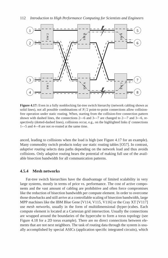
112 Introduction to High Performance Computing for Scientists and Engineers
1
3
4 8
7
6
5
2S
W 2
SW
1
SW
B
SW
4S
W 3
SW
A
Figure 4.17: Even in a fully nonblocking fat-tree switch hierarchy (network cabling shown assolid lines), not all possible combinations of N/2 point-to-point connections allow collision-free operation under static routing. When, starting from the collision-free connection patternshown with dashed lines, the connections 2↔6 and 3↔7 are changed to 2↔7 and 3↔6, re-spectively (dotted-dashed lines), collisions occur, e.g., on the highlighted links if connections1↔5 and 4↔8 are not re-routed at the same time.
anced, leading to collisions when the load is high (see Figure 4.17 for an example).Many commodity switch products today use static routing tables [O57]. In contrast,adaptive routing selects data paths depending on the network load and thus avoidscollisions. Only adaptive routing bears the potential of making full use of the avail-able bisection bandwidth for all communication patterns.
4.5.4 Mesh networks
Fat-tree switch hierarchies have the disadvantage of limited scalability in verylarge systems, mostly in terms of price vs. performance. The cost of active compo-nents and the vast amount of cabling are prohibitive and often force compromiseslike the reduction of bisection bandwidth per compute element. In order to overcomethose drawbacks and still arrive at a controllable scaling of bisection bandwidth, largeMPP machines like the IBM Blue Gene [V114, V115, V116] or the Cray XT [V117]use mesh networks, usually in the form of multidimensional (hyper-)cubes. Eachcompute element is located at a Cartesian grid intersection. Usually the connectionsare wrapped around the boundaries of the hypercube to form a torus topology (seeFigure 4.18 for a 2D torus example). There are no direct connections between ele-ments that are not next neighbors. The task of routing data through the system is usu-ally accomplished by special ASICs (application specific integrated circuits), which

Parallel computers 113
Figure 4.18: A two-dimensional (square)torus network. Bisection bandwidth scaleslike
√N in this case.
take care of all network traffic, bypassing the CPU whenever possible. The networkdiameter is the sum of the system’s sizes in all three Cartesian directions.
Certainly, bisection bandwidth does not scale linearly when enlarging the sys-tem in all dimensions but behaves like Bb(N) ∝ N(d−1)/d (d being the number ofdimensions), which leads to Bb(N)/N → 0 for large N. Maximum latency scales likeN1/d . Although these properties appear unfavorable at first sight, the torus topologyis an acceptable and extremely cost-effective compromise for the large class of ap-plications that are dominated by nearest-neighbor communication. If the maximumbandwidth per link is substantially larger than what a single compute element can“feed” into the network (its injection bandwidth), there is enough headroom to sup-port more demanding communication patterns as well (this is the case, for instance,on the Cray XT line of massively parallel computers [V117]). Another advantage ofa cubic mesh is that the amount of cabling is limited, and most cables can be keptshort. As with fat-tree networks, there is some heterogeneity in bandwidth and la-tency behavior, but if compute elements that work in parallel to solve a problem arelocated close together (i.e., in a cuboidal region), these characteristics are well pre-dictable. Moreover, there is no “arbitrary” system size at which bisection bandwidthper node suddenly has to drop due to cost and manageability concerns.
On smaller scales, simple mesh networks are used in shared-memory systems forccNUMA-capable connections between locality domains. Figure 4.19 shows an ex-ample of a four-socket server with HyperTransport interconnect. This node actuallyimplements a heterogeneous topology (in terms of intersocket latency) because twoHT connections are used for I/O connectivity: Any communication between the twolocality domains on the right incurs an additional hop via one of the other domains.
4.5.5 Hybrids
If a network is built as a combination of at least two of the topologies describedabove, it is called hybrid. In a sense, a cluster of shared-memory nodes like in Fig-

114 Introduction to High Performance Computing for Scientists and Engineers
Figure 4.19: A four-socket ccNUMA sys-tem with a HyperTransport-based meshnetwork. Each socket has only three HTlinks, so the network has to be heteroge-neous in order to accommodate I/O con-nections and still utilize all provided HTports.
I/O
I/O
HT
HT
HT
HT
HT
HT
HT
Memory
P P
Memory
P P
Memory
P P
Memory
P P
ure 4.8 implements a hybrid network even if the internode network itself is not hy-brid. This is because intranode connections tend to be buses (in multicore chips) orsimple meshes (for ccNUMA-capable fabrics like HyperTransport or QuickPath).On the large scale, using a cubic topology for node groups of limited size and a non-blocking fat tree further up reduces the bisection bandwidth problems of pure cubicmeshes.
Problems
For solutions see page 295 ff.
4.1 Building fat-tree network hierarchies. In a fat-tree network hierarchy withstatic routing, what are the consequences of a 2:3 oversubscription on the linksto the spine switches?
Chapter 5
Basics of parallelization
Before actually engaging in parallel programming it is vital to know about somefundamental rules in parallelization. This pertains to the available parallelization op-tions and, even more importantly, to performance limitations. It is one of the mostcommon misconceptions that the more “hardware” is put into executing a parallelprogram, the faster it will run. Billions of CPU hours are wasted every year becausesupercomputer users have no idea about the limitations of parallel execution.
In this chapter we will first identify and categorize the most common strategiesfor parallelization, and then investigate parallelism on a theoretical level: Simplemathematical models will be derived that allow insight into the factors that hamperparallel performance. Although the applicability and predictive power of such mod-els is limited, they provide unique insights that are largely independent of concreteparallel programming paradigms. Practical programming standards for writing par-allel programs will be introduced in the subsequent chapters.
5.1 Why parallelize?
With all the different kinds of parallel hardware that exists, from massively par-allel supercomputers down to multicore laptops, parallelism seems to be a ubiqui-tous phenomenon. However, many scientific users may even today not be requiredto actually write parallel programs, because a single core is sufficient to fulfill theirdemands. If such demands outgrow the single core’s capabilities, they can do so fortwo quite distinct reasons:
• A single core may be too slow to perform the required task(s) in a “tolerable”amount of time. The definition of “tolerable” certainly varies, but “overnight”is often a reasonable estimate. Depending on the requirements, “over lunch”or “duration of a PhD thesis” may also be valid.
• The memory requirements cannot be met by the amount of main memorywhich is available on a single system, because larger problems (with higherresolution, more physics, more particles, etc.) need to be solved.
The first problem is likely to occur more often in the future because of the irreversiblemulticore transition. For a long time, before the advent of parallel computers, the sec-ond problem was tackled by so-called out-of-core techniques, tailoring the algorithm
115
116 Introduction to High Performance Computing for Scientists and Engineers
so that large parts of the data set could be held on mass storage and loaded on demandwith a (hopefully) minor impact on performance. However, the chasm between peakperformance and available I/O bandwidth (and latency) is bound to grow even fasterthan the DRAM gap, and it is questionable whether out-of-core can play a major rolefor serial computing in the future. High-speed I/O resources in parallel computersare today mostly available in the form of parallel file systems, which unfold theirsuperior performance only if used with parallel data streams from different sources.
Of course, the reason for “going parallel” may strongly influence the chosenmethod of parallelization. The following section provides an overview on the latter.
5.2 Parallelism
Writing a parallel program must always start by identifying the parallelism in-herent in the algorithm at hand. Different variants of parallelism induce differentmethods of parallelization. This section can only give a coarse summary on availableparallelization methods, but it should enable the reader to consult more advancedliterature on the topic. Mattson et al. [S6] have given a comprehensive overview onparallel programming patterns. We will restrict ourselves to methods for exploitingparallelism using multiple cores or compute nodes. The fine-grained concurrency im-plemented with superscalar processors and SIMD capabilities has been introduced inChapters 1 and 2.
5.2.1 Data parallelism
Many problems in scientific computing involve processing of large quantities ofdata stored on a computer. If this manipulation can be performed in parallel, i.e., bymultiple processors working on different parts of the data, we speak of data paral-
lelism. As a matter of fact, this is the dominant parallelization concept in scientificcomputing on MIMD-type computers. It also goes under the name of SPMD (SingleProgram Multiple Data), as usually the same code is executed on all processors, withindependent instruction pointers. It is thus not to be confused with SIMD parallelism.
Example: Medium-grained loop parallelism
Processing of array data by loops or loop nests is a central component in mostscientific codes. A typical example are linear algebra operations on vectors or ma-trices, as implemented in the standard BLAS library [N50]. Often the computationsperformed on individual array elements are independent of each other and are hencetypical candidates for parallel execution by several processors in shared memory(see Figure 5.1). The reason why this variant of parallel computing is often called“medium-grained” is that the distribution of work across processors is flexible andeasily changeable down to the single data element: In contrast to what is shown in

Basics of parallelization 117
do i=1,500
a(i)=c*b(i)
enddo
do i=501,1000
a(i)=c*b(i)
enddo
a(i)=c*b(i)
do i=1,1000
enddo
P2
P1
Figure 5.1: An examplefor medium-grained par-allelism: The iterationsof a loop are distributedto two processors P1 andP2 (in shared memory)for concurrent execution.
Figure 5.1, one could choose an interleaved pattern where all odd-(even-)indexedelements are processed by P1 (P2).
OpenMP, a compiler extension based on directives and a simple API, supports,among other things, data parallelism on loops. See Chapter 6 for an introduction toOpenMP.
Example: Coarse-grained parallelism by domain decomposition
Simulations of physical processes (like, e.g., fluid flow, mechanical stress, quan-tum fields) often work with a simplified picture of reality in which a computational
domain, e.g., some volume of a fluid, is represented as a grid that defines discretepositions for the physical quantities under consideration (the Jacobi algorithm as in-troduced in Section 3.3 is an example). Such grids are not necessarily Cartesian butare often adapted to the numerical constraints of the algorithms used. The goal of thesimulation is usually the computation of observables on this grid. A straightforwardway to distribute the work involved across workers, i.e., processors, is to assign a partof the grid to each worker. This is called domain decomposition. As an example con-sider a two-dimensional Jacobi solver, which updates physical variables on a n× n
grid. Domain decomposition for N workers subdivides the computational domaininto N subdomains. If, e.g., the grid is divided into strips along the y direction (indexk in Listing 3.1), each worker performs a single sweep on its local strip, updatingthe array for time step T1. On a shared-memory parallel computer, all grid sites inall domains can be updated before the processors have to synchronize at the end ofthe sweep. However, on a distributed-memory system, updating the boundary sitesof one domain requires data from one or more adjacent domains. Therefore, before adomain update, all boundary values needed for the upcoming sweep must be commu-nicated to the relevant neighboring domains. In order to store this data, each domainmust be equipped with some extra grid points, the so-called halo or ghost layers (seeFigure 5.2). After the exchange, each domain is ready for the next sweep. The wholeparallel algorithm is completely equivalent to purely serial execution. Section 9.3will show in detail how this algorithm can be implemented using MPI, the MessagePassing Interface.
How exactly the subdomains should be formed out of the complete grid may be a

118 Introduction to High Performance Computing for Scientists and Engineers
Figure 5.2: Using halo (“ghost”) layersfor communication across domain bound-aries in a distributed-memory parallel Ja-cobi solver. After the local updates in eachdomain, the boundary layers (shaded) arecopied to the halo of the neighboring do-main (hatched).
������������
������������
���������������
���������������
���������������
���������������
������������
������������
������������
������������
���������������
���������������
���������������
���������������
������������
������������
���������������
���������������
���������������
���������������
������������
������������
������������
������������
���������������
���������������
���������������
���������������
�������������������������������������������
�������������������������������������������Domain 1
Domain 2
difficult problem to solve, because several factors influence the optimal choice. Firstand foremost, the computational effort should be equal for all domains to preventsome workers from idling while others still update their own domains. This is calledload balancing (see Figure 5.5 and Section 5.3.9). After load imbalance has beeneliminated one should care about reducing the communication overhead. The datavolume to be communicated is proportional to the overall area of the domain cuts.Comparing the two alternatives for 2D domain decomposition of an n×n grid to N
workers in Figure 5.3, one arrives at a communication cost of O (n(N −1)) for stripedomains, whereas an optimal decomposition into square subdomains leads to a costof O
(
2n(√
N −1))
. Hence, for large N the optimal decomposition has an advantagein communication cost of O
(
2/√
N)
. Whether this difference is significant or notin reality depends on the problem size and other factors, of course. Communicationmust be counted as overhead that reduces a program’s performance. In practice oneshould thus try to minimize boundary area as far as possible unless there are verygood reasons to do otherwise. See Section 10.4.1 for a more general discussion.
Note that the calculation of communication overhead depends crucially on thelocality of data dependencies, in the sense that communication cost grows linearlywith the distance that has to be bridged in order to calculate observables at a certainsite of the grid. For example, to get the first or second derivative of some quantitywith respect to the coordinates, only a next-neighbor relation has to be implementedand the communication layers in Figure 5.3 have a width of one. For higher-orderderivatives this changes significantly, and if there is some long-ranged interactionlike a Coulomb potential (1/distance), the layers would encompass the completecomputational domain, making communication dominant. In such a case, domaindecomposition is usually not applicable and one has to revert to other parallelizationstrategies.
Domain decomposition has the attractive property that domain boundary areagrows more slowly than volume if the problem size increases with N constant. There-

Basics of parallelization 119
Figure 5.3: Domain decomposition of a two-dimensional Jacobi solver, which requires next-neighbor interactions. Cutting into stripes (left) is simple but incurs more communication thanoptimal decomposition (right). Shaded cells participate in network communication.
fore, one can sometimes alleviate communication bottlenecks just by choosing alarger problem size. The expected effects of scaling problem size and/or the numberof workers with optimal domain decomposition in three dimensions will be discussedin Section 5.3 below.
The details about how the parallel Jacobi solver with domain decomposition canbe implemented in reality will be revealed in Section 9.3, after the introduction ofthe Message Passing Interface (MPI).
Although the Jacobi method is quite inefficient in terms of convergence proper-ties, it is very instructive and serves as a prototype for more advanced algorithms.Moreover, it lends itself to a host of scalar optimization techniques, some of whichhave been demonstrated in Section 3.4 in the context of matrix transposition (see alsoProblem 3.4 on page 92).
5.2.2 Functional parallelism
Sometimes the solution of a “big” numerical problem can be split into more orless disparate subtasks, which work together by data exchange and synchronization.In this case, the subtasks execute completely different code on different data items,which is why functional parallelism is also called MPMD (Multiple Program Mul-tiple Data). This does not rule out, however, that each subtask could be executed inparallel by several processors in an SPMD fashion.
Functional parallelism bears pros and cons, mainly because of performance rea-sons. When different parts of the problem have different performance properties andhardware requirements, bottlenecks and load imbalance can easily arise. On the otherhand, overlapping tasks that would otherwise be executed sequentially could accel-erate execution considerably.
In the face of the increasing number of processor cores on a chip to spend ondifferent tasks one may speculate whether we are experiencing the dawn of func-tional parallelism. In the following we briefly describe some important variants offunctional parallelism. See also Section 11.1.2 for another example in the context ofhybrid programming.

120 Introduction to High Performance Computing for Scientists and Engineers
Example: Master-worker scheme
Reserving one compute element for administrative tasks while all others solvethe actual problem is called the master-worker scheme. The master distributes workand collects results. A typical example is a parallel ray tracing program: A ray tracercomputes a photorealistic image from a mathematical representation of a scene. Foreach pixel to be rendered, a “ray” is sent from the imaginary observer’s eye into thescene, hits surfaces, gets reflected, etc., picking up color components. If all computeelements have a copy of the scene, all pixels are independent and can be computed inparallel. Due to efficiency concerns, the picture is usually divided into “work pack-ages” (rows or tiles). Whenever a worker has finished a package, it requests a new onefrom the master, who keeps lists of finished and yet to be completed tiles. In case ofa distributed-memory system, the finished tile must also be communicated over thenetwork. See Refs. [A80, A81] for an implementation and a detailed performanceanalysis of parallel raytracing in a master-worker setting.
A drawback of the master-worker scheme is the potential communication andperformance bottleneck that may appear with a single master when the number ofworkers is large.
Example: Functional decomposition
Multiphysics simulations are prominent applications for parallelization by func-tional decomposition. For instance, the airflow around a racing car could be simulatedusing a parallel CFD (Computational Fluid Dynamics) code. On the other hand, aparallel finite element simulation could describe the reaction of the flexible struc-tures of the car body to the flow, according to their geometry and material properties.Both codes have to be coupled using an appropriate communication layer.
Although multiphysics codes are gaining popularity, there is often a big load bal-ancing problem because it is hard in practice to dynamically shift resources betweenthe different functional domains. See Section 5.3.9 for more information on loadimbalance.
5.3 Parallel scalability
5.3.1 Factors that limit parallel execution
As shown in Section 5.2 above, parallelism may be exploited in a multitude ofways. Finding parallelism is not only a common problem in computing but also inmany other areas like manufacturing, traffic flow and even business processes. In avery simplistic view, all execution units (workers, assembly lines, waiting queues,CPUs,. . . ) execute their assigned work in exactly the same amount of time. Undersuch conditions, using N workers, a problem that takes a time T to be solved se-quentially will now ideally take only T/N (see Figure 5.4). We call this a speedup ofN.

Basics of parallelization 121
time
1 2 3 4 5 6 7 8 9 10 11 12
W1
W2
W3
time
2 3 4
8765
9 10 11 12
1
Figure 5.4: Parallelizing a sequence of tasks(top) using three workers (W1. . . W3) withperfect speedup (left).
Whatever parallelization scheme is chosen, this perfect picture will most prob-ably not hold in reality. Some of the reasons for this have already been mentionedabove: Not all workers might execute their tasks in the same amount of time becausethe problem was not (or could not) be partitioned into pieces with equal complex-ity. Hence, there are times when all but a few have nothing to do but wait for thelatecomers to arrive (see Figure 5.5). This load imbalance hampers performance be-cause some resources are underutilized. Moreover there might be shared resourceslike, e.g., tools that only exist once but are needed by all workers. This will effec-tively serialize part of the concurrent execution (Figure 5.6). And finally, the parallelworkflow may require some communication between workers, adding overhead thatwould not be present in the serial case (Figure 5.7). All these effects can imposelimits on speedup. How well a task can be parallelized is usually quantified by somescalability metric. Using such metrics, one can answer questions like:
• How much faster can a given problem be solved with N workers instead ofone?
• How much more work can be done with N workers instead of one?
• What impact do the communication requirements of the parallel applicationhave on performance and scalability?
• What fraction of the resources is actually used productively for solving theproblem?
The following sections introduce the most important metrics and develops modelsthat allow us to pinpoint the influence of some of the roadblocks just mentioned.
������������
��������
W1
W2
W3
time
1 2 3 4
5 6 7 8
1211109
Figure 5.5: Some tasks executed by dif-ferent workers at different speeds lead toload imbalance. Hatched regions indicateunused resources.

122 Introduction to High Performance Computing for Scientists and Engineers
Figure 5.6: Paralleli-zation with a bottleneck.Tasks 3, 7 and 11 cannotoverlap with anythingelse across the dashed“barriers.” time
W1
W2
W3
1
5
9 10
6
2 3
7
11 12
8
4
5.3.2 Scalability metrics
In order to be able to define scalability we first have to identify the basic mea-surements on which derived performance metrics are built. In a simple model, theoverall problem size (“amount of work”) shall be s + p = 1, where s is the serial(nonparallelizable) part and p is the perfectly parallelizable fraction. There can bemany reasons for a nonvanishing serial part:
• Algorithmic limitations. Operations that cannot be done in parallel because of,e.g., mutual dependencies, can only be performed one after another, or even ina certain order.
• Bottlenecks. Shared resources are common in computer systems: Executionunits in the core, shared paths to memory in multicore chips, I/O devices. Ac-cess to a shared resource serializes execution. Even if the algorithm itself couldbe performed completely in parallel, concurrency may be limited by bottle-necks.
• Startup overhead. Starting a parallel program, regardless of the technical de-tails, takes time. Of course, system designs try to minimize startup time, espe-cially in massively parallel systems, but there is always a nonvanishing serialpart. If a parallel application’s overall runtime is too short, startup will have astrong impact.
• Communication. Fully concurrent communication between different parts ofa parallel system cannot be taken for granted, as was shown in Section 4.5.If solving a problem in parallel requires communication, some serializationis usually unavoidable. We will see in Section 5.3.6 below how to incorpo-rate communication into scalability metrics in a more elaborate way than justadding a constant to the serial fraction.
Figure 5.7: Communication pro-cesses (arrows represent messages)limit scalability if they cannot beoverlapped with each other or withcalculation.
W3
W2
W1
time
1 2 3 4
8765
9 10 11 12
Basics of parallelization 123
First we assume a fixed problem, which is to be solved by N workers. We normalizethe single-worker (serial) runtime
T sf = s+ p (5.1)
to one. Solving the same problem on N workers will require a runtime of
Tp
f = s+p
N. (5.2)
This is called strong scaling because the amount of work stays constant no matterhow many workers are used. Here the goal of parallelization is minimization of timeto solution for a given problem.
If time to solution is not the primary objective because larger problem sizes (forwhich available memory is the limiting factor) are of interest, it is appropriate toscale the problem size with some power of N so that the total amount of work iss+ pNα , where α is a positive but otherwise free parameter. Here we use the implicitassumption that the serial fraction s is a constant. We define the serial runtime for thescaled (variably-sized) problem as
T sv = s+ pNα . (5.3)
Consequently, the parallel runtime is
T pv = s+ pNα−1 . (5.4)
The term weak scaling has been coined for this approach, although it is commonlyused only for the special case α = 1. One should add that other ways of scaling workwith N are possible, but the Nα dependency will suffice for what we want to showfurther on.
We will see that different scalability metrics with different emphasis on what“performance” really means can lead to some counterintuitive results.
5.3.3 Simple scalability laws
In a simple ansatz, application speedup can be defined as the quotient of paralleland serial performance for fixed problem size. In the following we define “perfor-mance” as “work over time,” unless otherwise noted. Serial performance for fixedproblem size (work) s+ p is thus
Psf =
s+ p
T sf
= 1 , (5.5)
as expected. Parallel performance is in this case
Ppf =
s+ p
Tp
f (N)=
1
s+ 1−sN
, (5.6)

124 Introduction to High Performance Computing for Scientists and Engineers
and application speedup (“scalability”) is
Sf =P
pf
Psf
=1
s+ 1−sN
“Amdahl’s Law” (5.7)
We have derived Amdahl’s Law, which was first conceived by Gene Amdahl in1967 [M45]. It limits application speedup for N → ∞ to 1/s. This well-known func-tion answers the question “How much faster (in terms of runtime) does my appli-cation run when I put the same problem on N CPUs?” As one might imagine, theanswer to this question depends heavily on how the term “work” is defined. If, incontrast to what has been done above, we define “work” as only the parallelizablepart of the calculation (for which there may be sound reasons at first sight), the resultsfor constant work are slightly different. Serial performance is
Pspf =
p
T sf
= p , (5.8)
and parallel performance is
Ppp
f =p
Tp
f (N)=
1− s
s+ 1−sN
. (5.9)
Calculation of application speedup finally yields
Spf =
Ppp
f
Pspf
=1
s+ 1−sN
, (5.10)
which is Amdahl’s Law again. Strikingly, Ppp
f and Spf (N) are not identical any more.
Although scalability does not change with this different notion of “work,” perfor-
mance does, and is a factor of p smaller.In the case of weak scaling where workload grows with CPU count, the question
to ask is “How much more work can my program do in a given amount of time whenI put a larger problem on N CPUs?” Serial performance as defined above is again
Psv =
s+ p
T sf
= 1 , (5.11)
as N = 1. Based on (5.3) and (5.4), Parallel performance (work over time) is
Ppv =
s+ pNα
Tp
v (N)=
s+(1− s)Nα
s+(1− s)Nα−1 = Sv , (5.12)
again identical to application speedup. In the special case α = 0 (strong scaling) werecover Amdahl’s Law. With 0 < α < 1, we get for large CPU counts
SvN≫1−→ s+(1− s)Nα
s= 1+
p
sNα , (5.13)
which is linear in Nα . As a result, weak scaling allows us to cross the Amdahl Barrier

Basics of parallelization 125
and get unlimited performance, even for small α . In the ideal case α = 1, (5.12)simplifies to
Sv(α = 1) = s+(1− s)N , “Gustafson’s Law” (5.14)
and speedup is linear in N, even for small N. This is called Gustafson’s Law [M46].Keep in mind that the terms with N or Nα in the previous formulas always bear aprefactor that depends on the serial fraction s, thus a large serial fraction can lead toa very small slope.
As previously demonstrated with Amdahl scaling we will now shift our focusto the other definition of “work” that only includes the parallel fraction p. Serialperformance is
Pspv = p (5.15)
and parallel performance is
Pppv =
pNα
Tp
v (N)=
(1− s)Nα
s+(1− s)Nα−1 , (5.16)
which leads to an application speedup of
Spv =
Pppv
Pspv
=Nα
s+(1− s)Nα−1 . (5.17)
Not surprisingly, speedup and performance are again not identical and differ by afactor of p. The important fact is that, in contrast to (5.14), for α = 1 applicationspeedup becomes purely linear in N with a slope of one. So even though the overallwork to be done (serial and parallel part) has not changed, scalability as defined in(5.17) makes us believe that suddenly all is well and the application scales perfectly.If some performance metric is applied that is only relevant in the parallel part of theprogram (e.g., “number of lattice site updates” instead of “CPU cycles”), this mistakecan easily go unnoticed, and CPU power is wasted (see next section).
5.3.4 Parallel efficiency
In the light of the considerations about scalability, one other point of interest isthe question how effectively a given resource, i.e., CPU computational power, canbe used in a parallel program (in the following we assume that the serial part of theprogram is executed on one single worker while all others have to wait). Usually,parallel efficiency is then defined as
ε =performance on N CPUs
N× performance on one CPU=
speedupN
. (5.18)
We will only consider weak scaling, since the limit α → 0 will always recover theAmdahl case. In the case where “work” is defined as s+ pNα , we get
ε =Sv
N=
sN−α +(1− s)
sN1−α +(1− s). (5.19)

126 Introduction to High Performance Computing for Scientists and Engineers
Figure 5.8: Weak scaling with an inap-propriate definition of “work” that in-cludes only the parallelizable part. Al-though “work over time” scales perfectlywith CPU count, i.e., εp = 1, most of theresources (hatched boxes) are unused be-cause s ≫ p. ���
������������������������������������������������������������������������������������������������������
���������������������������������������������������������������������������������������������������������
����������������������������������������������������������������������
����������������������������������������������������������������������
����������������������������������������������������������������������
����������������������������������������������������������������������
����������������������������������������������������������������������
����������������������������������������������������������������������
54321CPU#
p p p p p
s
For α = 0 this yields 1/(sN +(1− s)), which is the expected ratio for the Amdahlcase and approaches zero with large N. For α = 1 we get s/N + (1− s), which isalso correct because the more CPUs are used the more CPU cycles are wasted, and,starting from ε = s+ p = 1 for N = 1, efficiency reaches a limit of 1−s = p for largeN. Weak scaling enables us to use at least a certain fraction of CPU power, evenwhen the CPU count is very large. Wasted CPU time grows linearly with N, though,but this issue is clearly visible with the definitions used.
Results change completely when our other definition of “work” (pNα ) is applied.Here,
εp =S
pv
N=
Nα−1
s+(1− s)Nα−1 . (5.20)
For α = 1 we now get εp = 1, which should mean perfect efficiency. We are fooledinto believing that no cycles are wasted with weak scaling, although if s is large mostof the CPU power is unused. A simple example will exemplify this danger: Assumethat some code performs floating-point operations only within its parallelized part,which takes about 10% of execution time in the serial case. Using weak scalingwith α = 1, one could now report MFlops/sec performance numbers vs. CPU count(see Figure 5.8). Although all processors except one are idle 90% of their time, theMFlops/sec rate is a factor of N higher when using N CPUs. Performance behaviorthat is presented in this way should always raise suspicion.
5.3.5 Serial performance versus strong scalability
In order to check whether some performance model is appropriate for the codeat hand, one should measure scalability for some processor numbers and fix the freemodel parameters by least-squares fitting. Figure 5.9 shows an example where the

Basics of parallelization 127
2 4 6 8 10 12# cores
0
1
2
3
4
5
6
7
Re
lative
pe
rfo
rma
nce
Amdahl s = 0.168
Amdahl s = 0.086
Architecture 1
Architecture 2
Figure 5.9: Perfor-mance of a benchmarkcode versus the numberof processors (strongscaling) on two differentarchitectures. Althoughthe single-thread perfor-mance is nearly identicalon both machines, theserial fraction s is muchsmaller on architecture2, leading to superiorstrong scalability.
same code was run in a strong scaling scenario on two different parallel architectures.The measured performance data was normalized to the single-core case on architec-ture 1, and the serial fraction s was determined by a least-squares fit to Amdahl’sLaw (5.7).
Judging from the small performance difference on a single core it is quite surpris-ing that architecture 2 shows such a large advantage in scalability, with only abouthalf the serial fraction. This behavior can be explained by the fact that the parallelpart of the calculation is purely compute-bound, whereas the serial part is limitedby memory bandwidth. Although the peak performance per core is identical on bothsystems, architecture 2 has a much wider path to memory. As the number of work-ers increases, performance ceases to be governed by computational speed and thememory-bound serial fraction starts to dominate. Hence, the significant advantagein scalability for architecture 2. This example shows that it is vital to not only beaware of the existence of a nonparallelizable part but also of its specific demands onthe architecture under consideration: One should not infer the scalability behavior onone architecture from data obtained on the other. One may also argue that parallelcomputers that are targeted towards strong scaling should have a heterogeneous ar-chitecture, with some of the hardware dedicated exclusively to executing serial codeas fast as possible. This pertains to multicore chips as well [R39, M47, M48].
In view of optimization, strong scaling has the unfortunate side effect that usingmore and more processors leads to performance being governed by code that wasnot subject to parallelization efforts (this is one variant of the “law of diminishingreturns”). If standard scalar optimizations like those shown in Chapters 2 and 3 canbe applied to the serial part of an application, they can thus truly improve strongscalability, although serial performance will hardly change. The question whetherone should invest scalar optimization effort into the serial or the parallel part of anapplication seems to be answered by this observation. However, one must keep inmind that performance, and not scalability is the relevant metric; fortunately, Am-dahl’s Law can provide an approximate guideline. Assuming that the serial part can

128 Introduction to High Performance Computing for Scientists and Engineers
be accelerated by a factor of ξ > 1, parallel performance (see (5.6)) becomes
Ps,ξf =
1sξ
+ 1−sN
. (5.21)
On the other hand, if only the parallel part gets optimized (by the same factor) weget
Pp,ξf =
1
s+ 1−sξN
. (5.22)
The ratio of those two expressions determines the crossover point, i.e., the numberof workers at which optimizing the serial part pays off more:
Ps,ξf
Pp,ξf
=ξ s+ 1−s
N
s+ξ 1−sN
≥ 1 =⇒ N ≥ 1s−1 . (5.23)
This result does not depend on ξ , and it is exactly the number of workers where thespeedup is half the maximum asymptotic value predicted by Amdahl’s Law. If s≪ 1,parallel efficiency ε = (1− s)−1/2 is already close to 0.5 at this point, and it wouldnot make sense to enlarge N even further anyway. Thus, one should try to optimizethe parallelizable part first, unless the code is used in a region of very bad parallelefficiency (probably because the main reason for going parallel was lack of memory).
Note, however, that in reality it will not be possible to achieve the same speedupξ for both the serial and the parallel part, so the crossover point will be shifted ac-cordingly. In the example above (see Figure 5.9) the parallel part is dominated bymatrix-matrix multiplications, which run close to peak performance anyway. Accel-erating the sequential part is hence the only option to improve performance at a givenN.
5.3.6 Refined performance models
There are situations where Amdahl’s and Gustafson’s Laws are not appropriatebecause the underlying model does not encompass components like communication,load imbalance, parallel startup overhead, etc. As an example for possible refine-ments we will include a basic communication model. For simplicity we presupposethat communication cannot be overlapped with computation (see Figure 5.7), an as-sumption that is actually true for many parallel architectures. In a parallel calculation,communication must thus be accounted for as a correction term in parallel runtime(5.4):
T pcv = s+ pNα−1 + cα(N) . (5.24)
The communication overhead cα(N) must not be included into the definition of“work” that is used to derive performance as it emerges from processes that are solelya result of the parallelization. Parallel speedup is then
Scv =
s+ pNα
Tpc
v (N)=
s+(1− s)Nα
s+(1− s)Nα−1 + cα(N). (5.25)

Basics of parallelization 129
There are many possibilities for the functional dependence cα(N); it may be somesimple function, or it may not be possible to write it in closed form at all. Furthermorewe assume that the amount of communication is the same for all workers. As withprocessor-memory communication, the time a message transfer requires is the sumof the latency λ for setting up the communication and a “streaming” part κ = n/B,where n is the message size and B is the bandwidth (see Section 4.5.1 for real-worldexamples). A few special cases are described below:
• α = 0, blocking network: If the communication network has a “bus-like” struc-ture (see Section 4.5.2), i.e., only one message can be in flight at any time,and the communication overhead per CPU is independent of N then cα(N) =(κ +λ )N. Thus,
Scv =
1
s+ 1−sN
+(κ +λ )N
N≫1−→ 1(κ +λ )N
, (5.26)
i.e., performance is dominated by communication and even goes to zero forlarge CPU numbers. This is a very common situation as it also applies to thepresence of shared resources like memory paths, I/O devices and even on-chiparithmetic units.
• α = 0, nonblocking network, constant communication cost: If the communi-cation network can sustain N/2 concurrent messages with no collisions (seeSection 4.5.3), and message size is independent of N, then cα(N) = κ +λ and
Scv =
1
s+ 1−sN
+κ +λ
N≫1−→ 1s+κ +λ
. (5.27)
Here the situation is quite similar to the Amdahl case and performance willsaturate at a lower value than without communication.
• α = 0, nonblocking network, domain decomposition with ghost layer commu-
nication: In this case communication overhead decreases with N for strongscaling, e.g., like cα(N) = κN−β + λ . For any β > 0 performance at large N
will be dominated by s and the latency:
Scv =
1
s+ 1−sN
+κN−β +λ
N≫1−→ 1s+λ
. (5.28)
This arises, e.g., when domain decomposition (see page 117) is employed ona computational domain along all three coordinate axes. In this case β = 2/3.
• α = 1, nonblocking network, domain decomposition with ghost layer commu-
nication: Finally, when the problem size grows linearly with N, one may endup in a situation where communication per CPU stays independent of N. Asthis is weak scaling, the numerator leads to linear scalability with an overallperformance penalty (prefactor):
Scv =
s+ pN
s+ p+κ +λN≫1−→ s+(1− s)N
1+κ +λ. (5.29)

130 Introduction to High Performance Computing for Scientists and Engineers
Figure 5.10: Predict-ed parallel scalabilityfor different modelsat s = 0.05. In gen-eral, κ = 0.005 andλ = 0.001 except for theAmdahl case, which isshown for reference.
1 10 100 1000N
1
2
4
8
16
Svc
Amdahl (α=κ=λ=0)
α=0, blocking
α=0, nonblocking
α=0, 3D domain dec., nonblocking
α=1, 3D domain dec., nonblocking
Figure 5.10 illustrates the four cases at κ = 0.005, λ = 0.001, and s = 0.05, andcompares with Amdahl’s Law. Note that the simplified models we have covered inthis section are far from accurate for many applications. As an example, consider anapplication that is large enough to not fit into a single processor’s cache but smallenough to fit into the aggregate caches of Nc CPUs. Performance limitations likeserial fractions, communication, etc., could then be ameliorated, or even overcom-pensated, so that Sc
v(N) > N for some range of N. This is called superlinear speedup
and can only occur if problem size grows more slowly than N, i.e., at α < 1. See alsoSection 6.2 and Problem 7.2.
One must also keep in mind that those models are valid only for N > 1 as there isusually no communication in the serial case. A fitting procedure that tries to fix theparameters for some specific code should thus ignore the point N = 1.
When running application codes on parallel computers, there is often the ques-tion about the “optimal” choice for N. From the user’s perspective, N should be aslarge as possible, minimizing time to solution. This would generally be a waste of re-sources, however, because parallel efficiency is low near the performance maximum.See Problem 5.2 for a possible cost model that aims to resolve this conflict. Note thatif the main reason for parallelization is the need for large memory, low efficiencymay be acceptable nevertheless.
5.3.7 Choosing the right scaling baseline
Today’s high performance computers are all massively parallel. In the previoussections we have described the different ways a parallel computer can be built: Thereare multicore chips, sitting in multisocket shared-memory nodes, which are againconnected by multilevel networks. Hence, a parallel system always comprises a num-ber of hierarchy levels. Scaling a parallel code from one to many CPUs can lead tofalse conclusions if the hierarchical structure is not taken into account.
Figure 5.11 shows an example for strong scaling of an application on a systemwith four processors per node. Assuming that the code follows a communication

Basics of parallelization 131
0 4 8 12 16Number of cores
1
2
3
4
Sp
ee
du
p
s=0.2, k=0
Scaling data
1 2 3 4
No. of nodes
1
2
s=0.01, k=0.05
1 2 3 4
No. of cores
1
1.5
2
Figure 5.11: Speedupversus number of CPUsused for a hypotheticalcode on a hierarchicalsystem with four CPUsper node. Dependingon the chosen scalingbaseline, fits to themodel (5.26) can lead tovastly different results.Right inset: Scalabilityacross nodes. Left inset:Scalability inside onenode.
model as in (5.26), a least-squares fitting was used to determine the serial fraction s
and the communication time per process, k = κ +λ (main panel). As there is only aspeedup of ≈ 4 at 16 cores, s = 0.2 does seem plausible, and communication appar-ently plays no significant role. However, the quality of the fit is mediocre, especiallyfor small numbers of cores. Thus one may arrive at the conclusion that scalability in-side a node is governed by factors different from serial fraction and communication,and that (5.26) is not valid for all numbers of cores. The right inset in Figure 5.11shows scalability data normalized to the 4-core (one-node) performance, i.e., we havechosen a different scaling baseline. Obviously the model (5.26) is well suited for thissituation and yields completely different fitting parameters, which indicate that com-munication plays a major role (s = 0.01, k = 0.05). The left inset in Figure 5.11extracts the intranode behavior only; the data is typical for a memory-bound situa-tion. On a node architecture as in Figure 4.4, using two cores on the same socket maylead to a bandwidth bottleneck, which is evident from the small speedup when goingfrom one to two cores. Using the second socket as well gives a strong performanceboost, however.
In conclusion, scalability on a given parallel architecture should always be re-ported in relation to a relevant scaling baseline. On typical compute clusters, whereshared-memory multiprocessor nodes are coupled via a high-performance intercon-nect, this means that intranode and internode scaling behavior should be strictlyseparated. This principle also applies to other hierarchy levels like in, e.g., mod-ern multisocket multicore shared memory systems (see Section 4.2), and even to thethe complex cache group and thread structure in current multicore processors (seeSection 1.4).
5.3.8 Case study: Can slower processors compute faster?
It is often stated that, all else being equal, using a slower processor in a parallelcomputer (or a less-optimized single processor code) improves scalability of applica-

132 Introduction to High Performance Computing for Scientists and Engineers
Figure 5.12: Solving the sameproblem on 2N slow CPUs (left)instead of N fast CPUs (right)may speed up time to solution ifcommunication overhead per CPUgoes down with rising N. µ = 2 isthe performance ratio between fastand slow CPU.
���������������
���������������
��������������������
��������������������
��������������������
��������������������
���������������
���������������
��������������������
��������������������
��������������������
��������������������
���������������
���������������
��������������������
��������������������
���������������
�����������������������������������
����������������������������������������
�����������������������������������
���������������
Tslow
N=8 µ=2
Tfast
calc
N=4 µ=1
comm
tions because the adverse effects of communication overhead are reduced in relationto “useful” computation. A “truly scalable” computer may thus be built from slowCPUs and a reasonable network. In order to find the truth behind this concept wewill establish a performance model for “slow” computers. In this context, “slow”shall mean that the baseline serial execution time is µ ≥ 1 instead of 1, i.e., CPUspeed is quantified as µ−1. Figure 5.12 demonstrates how “slow computing” maywork. If the same problem is solved by µN slow instead of N fast processors, overallruntime may be shortened if communication overhead per CPU goes down as well.How strong this effect is and whether it makes sense to build a parallel computerbased on it remains to be seen. Interesting questions to ask are:
1. Does it make sense to use µN “slow” processors instead of N standard CPUsin order to get better overall performance?
2. What conditions must be fulfilled by communication overhead to achieve bet-ter performance with slow processors?
3. Does the concept work in strong and weak scaling scenarios alike?
4. What is the expected performance gain?
5. Can a “slow” machine deliver more performance than a machine with standardprocessors within the same power envelope?
For the last question, in the absence of communication overhead we already know theanswer because the situation is very similar to the multicore transition whose conse-quences were described in Section 1.4. The additional inefficiencies connected withcommunication might change those results significantly, however. More importantly,the CPU cores only contribute a part of the whole system’s power consumption; a

Basics of parallelization 133
power/performance model that merely comprises the CPU components is necessar-ily incomplete and will be of very limited use. Hence, we will concentrate on theother questions. We already expect from Figure 5.12 that a sensible performancemodel must include a realistic communication component.
Strong scaling
Assuming a fixed problem size and a generic communication model as in (5.24),the speedup for the slow computer is
Sµ(N) =1
s+(1− s)/N + c(N)/µ. (5.30)
For µ > 1 and N > 1 this is clearly larger than Sµ=1(N) whenever c(N) 6= 0: Amachine with slow processors “scales better,” but only if there is communicationoverhead.
Of course, scalability alone is no appropriate measure for application perfor-
mance since it relates parallel performance to serial performance on one CPU of thesame speed µ−1. We want to compare the absolute performance advantage of µN
slow CPUs over N standard processors:
Asµ(N) :=
Sµ(µN)
µSµ=1(N)=
s+(1− s)/N + c(N)
µs+(1− s)/N + c(µN)(5.31)
If µ > 1, this is greater than one if
c(µN)− c(N) < −s(µ −1) . (5.32)
Hence, if we assume that the condition should hold for all µ , c(N) must be a decreas-ing function of N with a minimum slope. At s = 0 a negative slope is sufficient, i.e.,communication overhead must decrease if N is increased. This result was expectedfrom the simple observation in Figure 5.12.
In order to estimate the achievable gains we look at the special case of Carte-sian domain decomposition on a nonblocking network as in (5.28). The advantagefunction is then
Asµ(N) :=
Sµ(µN)
µSµ=1(N)=
s+(1− s)/N +λ +κN−β
µs+(1− s)/N +λ +κ(Nµ)−β(5.33)
We can distinguish several cases here:
• κ = 0: With no communication bandwidth overhead,
Asµ(N) =
s+(1− s)/N +λ
µs+(1− s)/N +λN→∞−−−→ s+λ
µs+λ, (5.34)
which is always smaller than one. In this limit there is no performance to begained with slow CPUs, and the pure power advantage from using many slowprocessors is even partly neutralized.

134 Introduction to High Performance Computing for Scientists and Engineers
• κ 6= 0, λ = 0: To leading order in N−β (5.33) can be approximated as
Asµ(N) =
1µs
(
s+κN−β (1−µ−β ))
+O(N−2β )N→∞−−−→ 1
µ. (5.35)
Evidently, s 6= 0 and κ 6= 0 lead to opposite effects: For very large N, the serialfraction dominates and Aµ(N) < 1. At smaller N, there may be a chance to getAs
µ(N) > 1 if s is not too large.
• s = 0: In a strong scaling scenario, this case is somewhat unrealistic. However,it is the limit in which a machine with slow CPUs performs best: The positiveeffect of the κ-dependent terms, i.e., the reduction of communication band-width overhead with increasing N, is large, especially if the latency is low:
Asµ(N) =
N−1 +λ +κN−β
N−1 +λ +κ(Nµ)−β
N→∞,λ>0−−−−−−→ 1+ (5.36)
In the generic case κ 6= 0, λ 6= 0 and 0 < β < 1 this function approaches 1from above as N → ∞ and has a maximum at NMA = (1−β )/βλ . Hence, thelargest possible advantage is
As,maxµ = As
µ(NMA) =1+κβ β Xβ−1
1+κβ β Xβ−1µ−β, with X =
λ
1−β. (5.37)
This approaches µβ as λ → 0. At the time of writing, typical “scalable” HPCsystems with slow CPUs operate at 2 . µ . 4, so for optimal 3D domaindecomposition along all coordinate axes (β = 2/3) the maximum theoreticaladvantage is 1.5 . As,max . 2.5.
It must be emphasized that the assumption s = 0 cannot really be upheld for strongscaling because its influence will dominate scalability in the same way as networklatency for large N. Thus, we must conclude that the region of applicability for “slow”machines is very narrow in strong scaling scenarios.
Even if it may seem technically feasible to take the limit of very large µ andachieve even grater gains, it must be stressed that applications must provide sufficientparallelism to profit from more and more processors. This does not only refer toAmdahl’s Law, which predicts that the influence of the serial fraction s, howeversmall it may be initially, will dominate as N increases (as shown in (5.34) and (5.35));in most cases there is some “granularity” inherent to the model used to implementthe numerics (e.g., number of fluid cells, number of particles, etc.), which strictlylimits the number of workers.
Strictly weak scaling
We choose Gustafson scaling (work ∝ N) and a generic communication model.The speedup function for the slow computer is
Sµ(N) =[s+(1− s)N]/(µ + c(N))
µ−1 =s+(1− s)N
1+ c(N)/µ, (5.38)

Basics of parallelization 135
which leads to the advantage function
Awµ (N) :=
Sµ(µN)
µSµ=1(N)=
[s+(1− s)µN] [1+ c(N)]
[s+(1− s)N] [µ + c(µN)]. (5.39)
Neglecting the serial part s, this is greater than one if c(N) > c(µN)/µ : Commu-nication overhead may even increase with N, but this increase must be slower thanlinear.
For a more quantitative analysis we turn again to the concrete case of Cartesiandomain decomposition, where weak scaling incurs communication overhead that isindependent of N as in (5.29). We choose λ̃ := κ +λ because the bandwidth overheadenters as latency. The speedup function for the slow computer is
Sµ(N) =s+(1− s)N
1+ λ̃ µ−1, (5.40)
hence the performance advantage is
Awµ (N) :=
Sµ(µN)
µSµ=1(N)=
(1+ λ̃ ) [s+(1− s)µN]
[(1− s)N + s] (λ̃ + µ). (5.41)
Again we consider special cases:
• λ̃ = 0: In the absence of communication overhead,
Awµ (N) =
(1− s)N + s/µ
(1− s)N + s= 1− µ −1
µNs+O(s2) , (5.42)
which is clearly smaller than one, as expected. The situation is very similar tothe strong scaling case (5.34).
• s = 0: With perfect parallelizability the performance advantage is always largerthan one for µ > 1, and independent of N:
Awµ (N) =
1+ λ̃
1+ λ̃/µ=
µ≫λ̃−−−→ 1+ λ̃λ̃≫1−−−→ µ
(5.43)
However, there is no significant gain to be expected for small λ̃ . Even if λ̃ = 1,i.e., if communication overhead is comparable to the serial runtime, we onlyget 1.33 . Aw . 1.6 in the typical range 2 . µ . 4.
In this scenario we have assumed that the “slow” machine with µ times more pro-cessors works on a problem which is µ times as large — hence the term “strictlyweak scaling.” We are comparing “fast” and “slow” machines across different prob-lem sizes, which may not be what is desirable in reality, especially because the actualruntime grows accordingly. From this point of view the performance advantage Aw
µ ,even if it can be greater than one, misses the important aspect of “time to solution.”This disadvantage could be compensated if Aw
µ . µ , but this is impossible accordingto (5.43).

136 Introduction to High Performance Computing for Scientists and Engineers
Modified weak scaling
In reality, one would rather scale the amount of work with N (the number ofstandard CPUs) instead of µN so that the amount of memory per slow CPU can be µtimes smaller. Indeed, this is the way such “scalable” HPC systems are usually built.The performance model thus encompasses both weak and strong scaling.
The advantage function to look at must separate the notions for “number of work-ers” and “amount of work.” Therefore, we start with the speedup function
Smodµ (N,W ) =
[s+(1− s)W ]/ [µs+ µ(1− s)W/N + c(N/W )]
[s+(1− s)]/µ
=s+(1− s)W
s+(1− s)W/N + c(N/W )µ−1 , (5.44)
where N is the number of workers and W denotes the amount of parallel work to bedone. This expression specializes to strictly weak scaling if W = N and c(1) = λ̃ .The term c(N/W ) reflects the strong scaling component, effectively reducing com-munication overhead when N > W . Now we can derive the advantage function formodified weak scaling:
Amodµ (N) :=
Smodµ (µN,N)
µSmodµ=1(N,N)
=1+ c(1)
1+ s(µ −1)+ c(µ). (5.45)
This is independent of N, which is not surprising since we keep the problem sizeconstant when going from N to µN workers. The condition for a true advantage isthe same as for strong scaling at N = 1 (see (5.32)):
c(µ)− c(1) < −s(µ −1) . (5.46)
In case of Cartesian domain decomposition we have c(µ) = λ +κµ−β , hence
Amodµ (N) =
1+λ +κ
1+ s(µ −1)+λ +κµ−β. (5.47)
For s = 0 and to leading order in κ and λ ,
Amodµ (N) = 1+
(
1−µ−β)
κ −(
1+ µ−β)
λκ +O(λ 2,κ2) , (5.48)
which shows that communication bandwidth overhead (κ) dominates the gain. Soin contrast to the strictly weak scaling case (5.43), latency enters only in a second-order term. Even for κ = 1, at λ = 0, β = 2/3 and 2 . µ . 4 we get 1.2 . Amod .
1.4. In general, in the limit of large bandwidth overhead and small latency, modifiedweak scaling is the favorable mode of operation for parallel computers with slowprocessors. The dependence on µ is quite weak, and the advantage goes to 1+ κ asµ → ∞.
In conclusion, we have found theoretical evidence that it can really be useful to

Basics of parallelization 137
build large machines with many slow processors. Together with the expected reduc-tion in power consumption vs. application performance, they may provide an attrac-tive solution to the “power-performance dilemma,” and the successful line of IBMBlue Gene supercomputers [V114, V115] shows that the concept works in practice.However, one must keep in mind that not all applications are well suited for mas-sive parallelism, and that compromises must be made that may impede scalability(e.g., building fully nonblocking fat-tree networks becomes prohibitively expensivein very large systems). The need for a “sufficiently” strong single chip prevails if all
applications are to profit from the blessings of Moore’s Law.
5.3.9 Load imbalance
Inexperienced HPC users usually try to find the reasons for bad scalability oftheir parallel programs in the hardware details of the platform used and the specificdrawbacks of the chosen parallelization method: Communication overhead, synchro-nization loss, false sharing, NUMA locality, bandwidth bottlenecks, etc. While allthese are possible reasons for bad scalability (and are covered in due detail else-where in this book), load imbalance is often overlooked. Load imbalance occurswhen synchronization points are reached by some workers earlier than by others (seeFigure 5.5), leading to at least one worker idling while others still do useful work.As a consequence, resources are underutilized.
The consequences of load imbalance are hard to characterize in a simple modelwithout further assumptions about the work distribution. Also, the actual impact onperformance is not easily judged: As Figure 5.13 shows, having a few workers thattake longer to reach the synchronization point (“laggers”) leaves the rest, i.e., themajority of workers, idling for some time, incurring significant loss. On the otherhand, a few “speeders,” i.e., workers that finish their tasks early, may be harmlessbecause the accumulated waiting time is negligible (see Figure 5.14).
The possible reasons for load imbalance are diverse, and can generally be di-vided into algorithmic issues, which should be tackled by choosing a modified orcompletely different algorithm, and optimization problems, which could be solvedby code changes only. Sometimes the two are not easily distinguishable:
• The method chosen for distributing work among the workers may not be com-patible with the structure of the problem. For example, in case of the blockedJDS sparse matrix-vector multiply algorithm introduced in Section 3.6.2, onecould go about and assign a contiguous chunk of the loop over blocks (loopvariable ib) to each worker. Owing to the JDS storage scheme, this could (de-pending on the actual matrix structure) cause load imbalance because the lastiterations of the ib loop work on the lower parts of the matrix, where the num-ber of diagonals is smaller. In this situation it might be better to use a cyclic oreven dynamic distribution. This is especially easy to do with shared-memoryparallel programming; see Section 6.1.6.
• No matter what variant of parallelism is exploited (see Section 5.2), it may notbe known at compile time how much time a “chunk” of work actually takes.

138 Introduction to High Performance Computing for Scientists and Engineers
������������������������������������������
������������������������������������������
������������������������������������������
������������������������������������������
�����������������������������������
�����������������������������������
time
Sync point
wait
work
work
work
work
wait
wait
Figure 5.13: Load imbalance with few(one in this case) “laggers”: A lot of re-sources are underutilized (hatched areas).
������������������������������
������������������������������
time
Sync point
wait
work
work
work
work
Figure 5.14: Load imbalance with few(one in this case) “speeders”: Underutiliza-tion may be acceptable.
For example, an algorithm that requires each worker to perform a number ofiterations in order to reach some convergence limit could be inherently loadimbalanced because a different number of iterations may be needed on eachworker.
• There may be a coarse granularity to the problem, limiting the available paral-lelism. This happens usually when the number of workers is not significantlysmaller than the number of work packages. Exploiting additional levels of par-allelism (if they exist) can help mitigate this problem.
• Although load imbalance is most often caused by uneven work distributionas described above, there may be other reasons. If a worker has to wait forresources like, e.g., I/O or communication devices, the time spent with suchwaiting does not count as useful work but can nevertheless lead to a delay,which turns the worker into a “lagger” (this is not to be confused with OS jitter;see below). Additionally, overhead of this kind is often statistical in nature,causing erratic load imbalance behavior.
If load imbalance is identified as a major performance problem, it should be checkedwhether a different strategy for work distribution could eliminate or at least reduceit. When a completely even distribution is impossible, it may suffice to get rid of“laggers” to substantially improve scalability. Furthermore, hiding I/O and commu-nication costs by overlapping with useful work are also possible means to avoid loadimbalance [A82].

Basics of parallelization 139
time
���������������
���������������
������������������
������������������������������������
������������������������������������������
(a)
������������������������
������������������������
������������������������
������������������������
������������������������
������������������������
������������������������
������������������������
������������������������
������������������������
������������������������
������������������������
������������������������
������������������������
������������������������
������������������������
������������������������
������������������������
������������������������
������������������������
������������������������
������������������������
������������������������
������������������������
������������������������
������������������������
������������������������
������������������������������������������������������������������������������������������������
������������������������������������������������������������������������������������������������
������������������������
������������������������
������������������������
������������������������
������������������������
������������������������������������������������
������������������������
������������������������
������������������������
������������������������
������������������������
������������������������
������������������������
������������������������
������������������������
������������������������
������������������������
������������������������
������������������������
������������������������
������������������������������������������������
������������������������������������������������
��������������������
��������������������
������������������������
������������������������
(b)
������������������������
������������������������
������������������������
������������������������
������������������������
������������������������
������������������������
������������������������
������������������������
������������������������
������������������������
������������������������
��������������������
��������������������
��������������������
��������������������
(c)
Figure 5.15: If an OS-related delay (cross-hatched boxes) occurs with some given probabilityper time, the impact on parallel performance may be small when the number of workers issmall (a). Increasing the number of workers (here in a weak scaling scenario) increases theprobability of the delay occurring before the next synchronization point, lengthening overallruntime (b). Synchronizing OS activity on all operating systems in the machine eliminates“OS jitter,” leading to improved performance (c). (Pictures adapted from [L77]).

140 Introduction to High Performance Computing for Scientists and Engineers
OS jitter
A peculiar and interesting source of load imbalance with surprising consequenceshas recently been identified in large-scale parallel systems built from commoditycomponents [L77]. Most standard installations of distributed-memory parallel com-puters run individual, independent operating system instances on all nodes. An oper-ating system has many routine chores, of which running user programs is only one.Whenever a regular task like writing to a log file, delivering performance metrics,flushing disk caches, starting cron jobs, etc., kicks in, a running application processmay be delayed by some amount. On the next synchronization point, this “lagger”will delay the parallel program slightly due to load imbalance, but this is usuallynegligible if it happens infrequently and the number of processes is small (see Fig-ure 5.15 (a)). Certainly, the exact delay will depend on the duration of the OS activityand the frequency of synchronizations.
Unfortunately, the situation changes when the number of workers is massivelyincreased. This is because “OS noise” is of statistical nature over all workers; themore workers there are, the larger the probability that a delay will occur between twosuccessive synchronization points. Load imbalance will thus start to happen morefrequently when the frequency of synchronization points in the code comes near theaverage frequency of noise-caused delays, which may be described as a “resonance”phenomenon [L77]. This is shown in Figure 5.15 (b) for a weak scaling scenario.Note that this effect is strictly limited to massively parallel systems; in practice, it willnot show up with only tens or even hundreds of compute nodes. There are sources ofperformance variability in those smaller systems, too, but they are unrelated to OSjitter.
Apart from trying to reduce OS activity as far as possible (by, e.g., deactivatingunused daemons, polling, and logging activities, or leaving one processor per nodefree for OS tasks), an effective means of reducing OS jitter is to synchronize unavoid-able periodic activities on all workers (see Figure 5.15 (c)). This aligns the delays onall workers at the same synchronization point, and the performance penalty is notlarger than in case (a). However, such measures are not standard procedures and re-quire substantial changes to the operating system. Still, as the number of cores andnodes in large-scale parallel computers continues to increase, OS noise containmentwill most probably soon be a common feature.
Problems
For solutions see page 296 ff.
5.1 Overlapping communication and computation. How would the strong scalinganalysis for slow processors in Section 5.3.8 qualitatively change if communi-cation could overlap with computation (assuming that the hardware supportsit and the algorithm is formulated accordingly)? Take into account that theoverlap may not be perfect if communication time exceeds computation time.
Basics of parallelization 141
5.2 Choosing an optimal number of workers. If the scalability characteristics ofa parallel program are such that performance saturates or even declines withgrowing N, the question arises what the “optimal” number of workers is. Usu-ally one would not want to choose the point where performance is at its max-imum (or close to saturation), because parallel efficiency will already be lowthere. What is needed is a “cost model” that discourages the use of too manyworkers. Most computing centers charge for compute time in units of CPU
wallclock hours, i.e., an N-CPU job running for a time Tw will be charged asan amount proportional to NTw. For the user, minimizing the product of wall-time (i.e., time to solution) and cost should provide a sensible balance. Derivea condition for the optimal number of workers Nopt, assuming strong scal-ing with a constant communication overhead (i.e., a latency-bound situation).What is the speedup with Nopt workers?
5.3 The impact of synchronization. Synchronizing all workers can be very time-consuming, since it incurs costs that are usually somewhere between logarith-mic and linear in the number of workers. What is the impact of synchronizationon strong and weak scalability?
5.4 Accelerator devices. Accelerator devices for standard compute nodes are be-coming increasingly popular today. A common variant of this idea is to outfitstandard compute nodes (comprising, e.g., two multicore chips) with specialhardware sitting in an I/O slot. Accelerator hardware is capable of executingcertain operations orders of magnitude faster than the host system’s CPUs, butthe amount of available memory is usually much smaller than the host’s. Port-ing an application to an accelerator involves identifying suitable code parts toexecute on the special hardware. If the speedup for the accelerated code partsis α , how much of the original code (in terms of runtime) must be ported to getat least 90% efficiency on the accelerator hardware? What is the significanceof the memory size restrictions?
5.5 Fooling the masses with performance data. The reader is strongly encouragedto read David H. Bailey’s humorous article “Twelve Ways to Fool the MassesWhen Giving Performance Results on Parallel Computers” [S7]. Although thepaper was written already in 1991, many of the points made are still highlyrelevant.


Chapter 6
Shared-memory parallel programmingwith OpenMP
In the multicore world, one-socket single-core systems have all but vanished exceptfor the embedded market. The price vs. performance “sweet spot” lies mostly in thetwo-socket regime, with multiple cores (and possibly multiple chips) on a socket.Parallel programming in a basic form should thus start at the shared-memory level,although it is entirely possible to run multiple processes without a concept of sharedmemory. See Chapter 9 for details on distributed-memory parallel programming.
However, shared-memory programming is not an invention of the multicore era.Systems with multiple (single-core) processors have been around for decades, andappropriate portable programming interfaces, most notably POSIX threads [P9], havebeen developed in the 1990s. The basic principles, limitations and bottlenecks ofshared-memory parallel programming are certainly the same as with any other paral-lel model (see Chapter 5), although there are some peculiarities which will be coveredin Chapter 7. The purpose of the current chapter is to give a nonexhaustive overviewof OpenMP, which is the dominant shared-memory programming standard today.OpenMP bindings are defined for the C, C++, and Fortran languages as of the cur-rent version of the standard (3.0). Some OpenMP constructs that are mainly used foroptimization will be introduced in Chapter 7.
We should add that there are specific solutions for the C++ language like, e.g.,Intel Threading Building Blocks (TBB) [P10], which may provide better function-ality than OpenMP in some respects. We also deliberately ignore compiler-basedautomatic shared-memory parallelization because it has up to now not lived up toexpectations except for trivial cases.
6.1 Short introduction to OpenMP
Shared memory opens the possibility to have immediate access to all data fromall processors without explicit communication. Unfortunately, POSIX threads are nota comfortable parallel programming model for most scientific software, which is typ-ically loop-centric. For this reason, a joint effort was made by compiler vendors toestablish a standard in this field, called OpenMP [P11]. OpenMP is a set of compiler
directives that a non-OpenMP-capable compiler would just regard as comments andignore. Hence, a well-written parallel OpenMP program is also a valid serial program
143

144 Introduction to High Performance Computing for Scientists and Engineers
Figure 6.1: Model for OpenMP thread op-erations: The master thread “forks” teamof threads, which work on shared memoryin a parallel region. After the parallel re-gion, the threads are “joined,” i.e., termi-nated or put to sleep, until the next par-allel region starts. The number of runningthreads may vary among parallel regions.
serial
region
parallel
region
team of
threads
master thread
fork
join
(this is certainly not a requirement, but it simplifies development and debugging con-siderably). The central entity in an OpenMP program is not a process but a thread.Threads are also called “lightweight processes” because several of them can sharea common address space and mutually access data. Spawning a thread is much lesscostly than forking a new process, because threads share everything but instructionpointer (the address of the next instruction to be executed), stack pointer and reg-ister state. Each thread can, by means of its local stack pointer, also have “private”variables, but since all data is accessible via the common address space, it is only amatter of taking the address of an item to make it accessible to all other threads aswell. However, the OpenMP standard actually forbids making a private object avail-able to other threads via its address. It will become clear later that this is actually agood idea.
We will concentrate on the Fortran interface for OpenMP here, and point outimportant differences to the C/C++ bindings as appropriate.
6.1.1 Parallel execution
In any OpenMP program, a single thread, the master thread, runs immediatelyafter startup. Truly parallel execution happens inside parallel regions, of which an ar-bitrary number can exist in a program. Between two parallel regions, no thread exceptthe master thread executes any code. This is also called the “fork-join model” (seeFigure 6.1). Inside a parallel region, a team of threads executes instruction streamsconcurrently. The number of threads in a team may vary among parallel regions.
OpenMP is a layer that adapts the raw OS thread interface to make it more us-

Shared-memory parallel programming with OpenMP 145
able with the typical structures that numerical software tends to employ. In prac-tice, parallel regions in Fortran are initiated by !$OMP PARALLEL and ended by!$OMP END PARALLEL directives, respectively. The !$OMP string is a so-calledsentinel, which starts an OpenMP directive (in C/C++, #pragma omp is used in-stead). Inside a parallel region, each thread carries a unique identifier, its thread ID,which runs from zero to the number of threads minus one, and can be obtained bythe omp_get_thread_num() API function:
1 use omp_lib ! module with API declarations
2
3 print *,’I am the master, and I am alone’
4 !$OMP PARALLEL
5 call do_work_package(omp_get_thread_num(),omp_get_num_threads())
6 !$OMP END PARALLEL
The omp_get_num_threads() function returns the number of active threads inthe current parallel region. The omp_lib module contains the API definitions (inFortran 77 and C/C++ there are include files mpif.h and omp.h, respectively).Code between OMP PARALLEL and OMP END PARALLEL, including subroutinecalls, is executed by every thread. In the simplest case, the thread ID can be usedto distinguish the tasks to be performed on different threads; this is done by callingthe do_work_package() subroutine in above example with the thread ID andthe overall number of threads as parameters. Using OpenMP in this way is mostlyequivalent to the POSIX threads programming model.
An important difference between the Fortran and C/C++ OpenMP bindings mustbe stressed here. In C/C++, there is no end parallel directive, because all direc-tives apply to the following statement or structured block. The example above wouldthus look like this in C++:
1 #include <omp.h>
2
3 std::cout << "I am the master, and I am alone";
4 #pragma omp parallel
5 {
6 do_work_package(omp_get_thread_num(),omp_get_num_threads());
7 }
The curly braces could actually be omitted in this particular case, but the fact that astructured block is subject to parallel execution has consequences for data scoping(see below).
The actual number of running threads does not have to be known at compile time.It can be set by the environment variable prior to running the executable:
1 $ export OMP_NUM_THREADS=4
2 $ ./a.out
Although there are also means to set or alter the number of running threads underprogram control, an OpenMP program should always be written so that it does notassume a specific number of threads.

146 Introduction to High Performance Computing for Scientists and Engineers
Listing 6.1: “Manual” loop parallelization and variable privatization. Note that this is not theintended mode for OpenMP.
1 integer :: bstart, bend, blen, numth, tid, i
2 integer :: N
3 double precision, dimension(N) :: a,b,c
4 ...
5 !$OMP PARALLEL PRIVATE(bstart,bend,blen,numth,tid,i)
6 numth = omp_get_num_threads()
7 tid = omp_get_thread_num()
8 blen = N/numth
9 if(tid.lt.mod(N,numth)) then
10 blen = blen + 1
11 bstart = blen * tid + 1
12 else
13 bstart = blen * tid + mod(N,numth) + 1
14 endif
15 bend = bstart + blen - 1
16 do i = bstart,bend
17 a(i) = b(i) + c(i)
18 enddo
19 !$OMP END PARALLEL
6.1.2 Data scoping
Any variables that existed before a parallel region still exist inside, and are bydefault shared between all threads. True work sharing, however, makes sense onlyif each thread can have its own, private variables. OpenMP supports this conceptby defining a separate stack for every thread. There are three ways to make privatevariables:
1. A variable that exists before entry to a parallel construct can be privatized, i.e.,made available as a private instance for every thread, by a PRIVATE clause tothe OMP PARALLEL directive. The private variable’s scope extends until theend of the parallel construct.
2. The index variable of a worksharing loop (see next section) is automaticallymade private.
3. Local variables in a subroutine called from a parallel region are private to eachcalling thread. This pertains also to copies of actual arguments generated bythe call-by-value semantics, and to variables declared inside structured blocksin C/C++. However, local variables carrying the SAVE attribute in Fortran (orthe static storage class in C/C++) will be shared.
Shared variables that are not modified in the parallel region do not have to be madeprivate.
A simple loop that adds two arrays could thus be parallelized as shown in List-ing 6.1. The actual loop is contained in lines 16–18, and everything before that is

Shared-memory parallel programming with OpenMP 147
just for calculating the loop bounds for each thread. In line 5 the PRIVATE clauseto the PARALLEL directive privatizes all specified variables, i.e., each thread gets itsown instance of each variable on its local stack, with an undefined initial value (C++objects will be instantiated using the default constructor). Using FIRSTPRIVATE
instead of PRIVATE would initialize the privatize instances with the contents of theshared instance (in C++, the copy constructor is employed). After the parallel region,the original values of the privatized variables are retained if they are not modified onpurpose. Note that there are separate clauses (THREADPRIVATE and COPYIN, re-spectively [P11]) for privatization of global or static data (SAVE variables, commonblock elements, static variables).
In C/C++, there is actually less need for using the private clause in manycases, because the parallel directive applies to a structured block. Instead ofprivatizing shared instances, one can simply declare local variables:
1 #pragma omp parallel
2 {
3 int bstart, bend, blen, numth, tid, i;
4 ... // calculate loop boundaries
5 for(i=bstart; i<=bend; ++i)
6 a[i] = b[i] + c[i];
7 }
Manual loop parallelization as shown here is certainly not the intended mode ofoperation in OpenMP. The standard defines much more advanced means of distribut-ing work among threads (see below).
6.1.3 OpenMP worksharing for loops
Being the omnipresent programming structure in scientific codes, loops are nat-ural candidates for parallelization if individual iterations are independent. This cor-responds to the medium-grained data parallelism described in Section 5.2.1. As anexample, consider a parallel version of a simple program for the calculation of π byintegration:
π =
1∫
0
dx4
1+ x2 (6.1)
Listing 6.2 shows a possible implementation. In contrast to the previous examples,this is also valid serial code. The initial value of sum is copied to the private instancesvia the FIRSTPRIVATE clause on the PARALLEL directive. Then, a DO directivein front of a do loop starts a worksharing construct: The iterations of the loop aredistributed among the threads (which are running because we are in a parallel region).Each thread gets its own iteration space, i.e., is assigned to a different set of i values.How threads are mapped to iterations is implementation-dependent by default, butcan be influenced by the programmer (see Section 6.1.6 below). Although shared inthe enclosing parallel region, the loop counter i is privatized automatically. The finalEND DO directive after the loop is not strictly necessary here, but may be requiredin cases where the NOWAIT clause is specified; see Section 7.2.1 on page 170 for

148 Introduction to High Performance Computing for Scientists and Engineers
Listing 6.2: A simple program for numerical integration of a function in OpenMP.
1 double precision :: pi,w,sum,x
2 integer :: i,N=1000000
3
4 pi = 0.d0
5 w = 1.d0/N
6 sum = 0.d0
7 !$OMP PARALLEL PRIVATE(x) FIRSTPRIVATE(sum)
8 !$OMP DO
9 do i=1,n
10 x = w*(i-0.5d0)
11 sum = sum + 4.d0/(1.d0+x*x)
12 enddo
13 !$OMP END DO
14 !$OMP CRITICAL
15 pi= pi + w*sum
16 !$OMP END CRITICAL
17 !$OMP END PARALLEL
details. A DO directive must be followed by a do loop, and applies to this loop only.In C/C++, the for directive serves the same purpose. Loop counters are restricted tointegers (signed or unsigned), pointers, or random access iterators.
In a parallel loop, each thread executes “its” share of the loop’s iteration space,accumulating into its private sum variable (line 11). After the loop, and still insidethe parallel region, the partial sums must be added to get the final result (line 15),because the private instances of sum will be gone once the region is left. There is aproblem, however: Without any countermeasures, threads would write to the resultvariable pi concurrently. The result would depend on the exact order the threadsaccess pi, and it would most probably be wrong. This is called a race condition, andthe next section will explain what one can do to prevent it.
Loop worksharing works even if the parallel loop itself resides in a subroutinecalled from the enclosing parallel region. The DO directive is then called orphaned,because it is outside the lexical extent of a parallel region. If such a directive isencountered while no parallel region is active, the loop will not be workshared.
Finally, if a separation of the parallel region from the workshared loop is notrequired, the two directives can be combined:
1 !$OMP PARALLEL DO
2 do i=1,N
3 a(i) = b(i) + c(i) * d(i)
4 enddo
5 !$OMP END PARALLEL DO
The set of clauses allowed for this combined parallel worksharing directive is theunion of all clauses allowed on each directive separately.
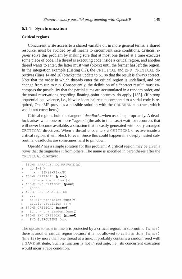
Shared-memory parallel programming with OpenMP 149
6.1.4 Synchronization
Critical regions
Concurrent write access to a shared variable or, in more general terms, a sharedresource, must be avoided by all means to circumvent race conditions. Critical re-
gions solve this problem by making sure that at most one thread at a time executessome piece of code. If a thread is executing code inside a critical region, and anotherthread wants to enter, the latter must wait (block) until the former has left the region.In the integration example (Listing 6.2), the CRITICAL and END CRITICAL di-rectives (lines 14 and 16) bracket the update to pi so that the result is always correct.Note that the order in which threads enter the critical region is undefined, and canchange from run to run. Consequently, the definition of a “correct result” must en-compass the possibility that the partial sums are accumulated in a random order, andthe usual reservations regarding floating-point accuracy do apply [135]. (If strongsequential equivalence, i.e., bitwise identical results compared to a serial code is re-quired, OpenMP provides a possible solution with the ORDERED construct, whichwe do not cover here.)
Critical regions hold the danger of deadlocks when used inappropriately. A dead-lock arises when one or more “agents” (threads in this case) wait for resources thatwill never become available, a situation that is easily generated with badly arrangedCRITICAL directives. When a thread encounters a CRITICAL directive inside acritical region, it will block forever. Since this could happen in a deeply nested sub-routine, deadlocks are sometimes hard to pin down.
OpenMP has a simple solution for this problem: A critical region may be given aname that distinguishes it from others. The name is specified in parentheses after theCRITICAL directive:
1 !$OMP PARALLEL DO PRIVATE(x)
2 do i=1,N
3 x = SIN(2*PI*x/N)
4 !$OMP CRITICAL (psum)
5 sum = sum + func(x)
6 !$OMP END CRITICAL (psum)
7 enddo
8 !$OMP END PARALLEL DO
9 ...
10 double precision func(v)
11 double precision :: v
12 !$OMP CRITICAL (prand)
13 func = v + random_func()
14 !$OMP END CRITICAL (prand)
15 END SUBROUTINE func
The update to sum in line 5 is protected by a critical region. In subroutine func()there is another critical region because it is not allowed to call random_func()(line 13) by more than one thread at a time; it probably contains a random seed witha SAVE attribute. Such a function is not thread safe, i.e., its concurrent executionwould incur a race condition.
150 Introduction to High Performance Computing for Scientists and Engineers
Without the names on the two different critical regions, this code would deadlockbecause a thread that has just called func(), already in a critical region, wouldimmediately encounter the second critical region and wait for itself indefinitely tofree the resource. With the names, the second critical region is understood to protecta different resource than the first.
A disadvantage of named critical regions is that the names are unique identifiers.It is not possible to have them indexed by an integer variable, for instance. There areOpenMP API functions that support the use of locks for protecting shared resources.The advantage of locks is that they are ordinary variables that can be arranged asarrays or in structures. That way it is possible to protect each single element of anarray of resources individually, even if their number is not known at compile time.See Section 7.2.3 for an example.
Barriers
If, at a certain point in the parallel execution, it is necessary to synchronize all
threads, a BARRIER can be used:
1 !$OMP BARRIER
The barrier is a synchronization point, which guarantees that all threads have reachedit before any thread goes on executing the code below it. Certainly it must be ensuredthat every thread hits the barrier, or a deadlock may occur.
Barriers should be used with caution in OpenMP programs, partly because oftheir potential to cause deadlocks, but also due to their performance impact (syn-chronization is overhead). Note also that every parallel region executes an implicitbarrier at its end, which cannot be removed. There is also a default implicit barrier atthe end of worksharing loops and some other constructs to prevent race conditions.It can be eliminated by specifying the NOWAIT clause. See Section 7.2.1 for details.
6.1.5 Reductions
The example in Listing 6.3 shows a loop code that adds some random noise to theelements of an array a() and calculates its vector norm. The RANDOM_NUMBER()subroutine may be assumed to be thread safe, according to the OpenMP standard.
Similar to the integration code in Listing 6.2, the loop implements a reduction
operation: Many contributions (the updated elements of a()) are accumulated intoa single variable. We have previously solved this problem with a critical region, butOpenMP provides a more elegant alternative by supporting reductions directly viathe REDUCTION clause (end of line 5). It automatically privatizes the specified vari-able(s) (s in this case) and initializes the private instances with a sensible startingvalue. At the end of the construct, all partial results are accumulated into the sharedinstance of s, using the specified operator (+ here) to get the final result.
There is a set of supported operators for OpenMP reductions (slightly differentfor Fortran and C/C++), which cannot be extended. C++ overloaded operators arenot allowed. However, the most common cases (addition, subtraction, multiplication,

Shared-memory parallel programming with OpenMP 151
Listing 6.3: Example with reduction clause for adding noise to the elements of an array andcalculating its vector norm.
1 double precision :: r,s
2 double precision, dimension(N) :: a
3
4 call RANDOM_SEED()
5 !$OMP PARALLEL DO PRIVATE(r) REDUCTION(+:s)
6 do i=1,N
7 call RANDOM_NUMBER(r) ! thread safe
8 a(i) = a(i) + func(r) ! func() is thread safe
9 s = s + a(i) * a(i)
10 enddo
11 !$OMP END PARALLEL DO
12
13 print *,’Sum = ’,s
logical, etc.) are covered. If a required operator is not available, one must revert tothe “manual” method as shown in the Listing 6.2.
Note that the automatic initialization for reduction variables, though convenient,bears the danger of producing invalid serial, i.e., non-OpenMP code. Compiling theexample above without OpenMP support will leave s uninitialized.
6.1.6 Loop scheduling
As mentioned earlier, the mapping of loop iterations to threads is configurable. Itcan be controlled by the argument of a SCHEDULE clause to the loop worksharingdirective:
1 !$OMP DO SCHEDULE(STATIC)
2 do i=1,N
3 a(i) = calculate(i)
4 enddo
5 !$OMP END DO
The simplest possibility is STATIC, which divides the loop into contiguous chunksof (roughly) equal size. Each thread then executes on exactly one chunk. If for somereason the amount of work per loop iteration is not constant but, e.g., decreases withloop index, this strategy is suboptimal because different threads will get vastly dif-ferent workloads, which leads to load imbalance. One solution would be to use achunksize like in “STATIC,1,” dictating that chunks of size 1 should be distributedacross threads in a round-robin manner. The chunksize may not only be a constantbut any valid integer-valued expression.
There are alternatives to the static schedule for other types of workload (see Fig-ure 6.2). Dynamic scheduling assigns a chunk of work, whose size is defined by thechunksize, to the next thread that has finished its current chunk. This allows for avery flexible distribution which is usually not reproduced from run to run. Threadsthat get assigned “easier” chunks will end up completing more of them, and load

152 Introduction to High Performance Computing for Scientists and Engineers
���������
������������������
������������������
���������
������������
������������
������������
������������
���������
���������
���������
���������
���������
���������
������������
������������
������������
������
������
������
������
������
������
��������
��������
��������
��������
������
������
������
������
������
������
������
������
��������
��������
���������
���������
������
������
������
������
������
������
��������
��������
��������
STATIC STATIC,3 DYNAMIC[,1] DYNAMIC,3
T0
T1
T2
1
2
3
4
5
6
7
8
9
10
11
12
13
14
15
16
17
18
19
20
Iteration
GUIDED[,1]
Figure 6.2: Loop schedules in OpenMP. The example loop has 20 iterations and is executedby three threads (T0, T1, T2). The default chunksize for DYNAMIC and GUIDED is one. If achunksize is specified, the last chunk may be shorter. Note that only the STATIC schedulesguarantee that the distribution of chunks among threads stays the same from run to run.
imbalance is greatly reduced. The downside is that dynamic scheduling generatessignificant overhead if the chunks are too small in terms of execution time (see Sec-tion 7.2.1 for an assessment of scheduling overhead). This is why it is often desirableto use a moderately large chunksize on tight loops, which in turn leads to more loadimbalance. In cases where this is a problem, the guided schedule may help. Again,threads request new chunks dynamically, but the chunksize is always proportional tothe remaining number of iterations divided by the number of threads. The smallestchunksize is specified in the schedule clause (default is 1). Despite the dynamic as-signment of chunks, scheduling overhead is kept under control. However, a word ofcaution is in order regarding dynamic and guided schedules: Due to the indetermin-istic nature of the assignment of threads to chunks, applications that are limited bymemory bandwidth may suffer from insufficient access locality on ccNUMA systems(see Section 4.2.3 for an introduction to ccNUMA architecture and Chapter 8 forccNUMA-specific performance effects and optimization methods). The static sched-ule is thus the only choice under such circumstances, if the standard worksharing

Shared-memory parallel programming with OpenMP 153
directives are used. Of course there is also the possibility of “explicit” scheduling,using the thread ID number to assign work to threads as shown in Section 6.1.2.
For debugging and profiling purposes, OpenMP provides a facility to determinethe loop scheduling at runtime. If the scheduling clause specifies “RUNTIME,” theloop is scheduled according to the contents of the OMP_SCHEDULE shell variable.However, there is no way to set different schedulings for different loops that use theSCHEDULE(RUNTIME) clause.
6.1.7 Tasking
In early versions of the standard, parallel worksharing in OpenMP was mainlyconcerned with loop structures. However, not all parallel work comes in loops; a typ-ical example is a linear list of objects (probably arranged in a std::list<> STLcontainer), which should be processed in parallel. Since a list is not easily address-able by an integer index or a random-access iterator, a loop worksharing construct isruled out, or could only be used with considerable programming effort.
OpenMP 3.0 provides the task concept to circumvent this limitation. A task isdefined by the TASK directive, and contains code to be executed.1 When a threadencounters a task construct, it may execute it right away or set up the appropriatedata environment and defer its execution. The task is then ready to be executed laterby any thread of the team.
As a simple example, consider a loop in which some function must be called foreach loop index with some probability:
1 integer i,N=1000000
2 type(object), dimension(N) :: p
3 double precision :: r
4 ...
5 !$OMP PARALLEL PRIVATE(r,i)
6 !$OMP SINGLE
7 do i=1,N
8 call RANDOM_NUMBER(r)
9 if(p(i)%weight > r) then
10 !$OMP TASK
11 ! i is automatically firstprivate
12 ! p() is shared
13 call do_work_with(p(i))
14 !$OMP END TASK
15 endif
16 enddo
17 !$OMP END SINGLE
18 !$OMP END PARALLEL
The actual number of calls to do_work_with() is unknown, so tasking is a nat-ural choice here. A do loop over all elements of p() is executed in a SINGLE
region (lines 6–17). A SINGLE region will be entered by one thread only, namelythe one that reaches the SINGLE directive first. All others skip the code until the
1In OpenMP terminology, “task” is actually a more general term; the definition given here is sufficientfor our purpose.

154 Introduction to High Performance Computing for Scientists and Engineers
END SINGLE directive and wait there in an implicit barrier. With a probability de-termined by the current object’s content, a TASK construct is entered. One task con-sists in the call to do_work_with() (line 13) together with the appropriate dataenvironment, which comprises the array of types p() and the index i. Of course, theindex is unique for each task, so it should actually be subject to a FIRSTPRIVATEclause. OpenMP specifies that variables that are private in the enclosing context areautomatically made FIRSTPRIVATE inside the task, while shared data stays shared(except if an additional data scoping clause is present). This is exactly what we wanthere, so no additional clause is required.
All the tasks generated by the thread in the SINGLE region are subject to dy-namic execution by the thread team. Actually, the generating thread may also beforced to suspend execution of the loop at the TASK construct (which is one exam-ple of a task scheduling point) in order to participate in running queued tasks. Thiscan happen when the (implementation-dependent) internal limit of queued tasks isreached. After some tasks have been run, the generating thread will return to theloop. Note that there are complexities involved in task scheduling that our simpleexample cannot fathom; multiple threads can generate tasks concurrently, and taskscan be declared untied so that a different thread may take up execution at a taskscheduling point. The OpenMP standard provides excessive examples.
Task parallelism with its indeterministic execution poses the same problems forccNUMA access locality as dynamic or guided loop scheduling. Programming tech-niques to ameliorate these difficulties do exist [O58], but their applicability is limited.
6.1.8 Miscellaneous
Conditional compilation
In some cases it may be useful to write different code depending on OpenMP be-ing enabled or not. The directives themselves are no problem here because they willbe ignored gracefully. Beyond this default behavior one may want to mask out, e.g.,calls to API functions or any code that makes no sense without OpenMP enabled.This is supported in C/C++ by the preprocessor symbol _OPENMP, which is definedonly if OpenMP is available. In Fortran the special sentinel “!$” acts as a commentonly if OpenMP is not enabled (see Listing 6.4).
Memory consistency
In the code shown in Listing 6.4, the second API call (line 8) is located in aSINGLE region. This is done because numthreads is global and should be writtento only by one thread. In the critical region each thread just prints a message, but anecessary requirement for the numthreads variable to have the updated value isthat no thread leaves the SINGLE region before the update has been “promoted” tomemory. The END SINGLE directive acts as an implicit barrier, i.e., no thread cancontinue executing code before all threads have reached the same point. The OpenMPmemory model ensures that barriers enforce memory consistency: Variables that havebeen held in registers are written out so that cache coherence can make sure that

Shared-memory parallel programming with OpenMP 155
Listing 6.4: Fortran sentinels and conditional compilation with OpenMP combined.
1 !$ use omp_lib
2 myid=0
3 numthreads=1
4 #ifdef _OPENMP
5 !$OMP PARALLEL PRIVATE(myid)
6 myid = omp_get_thread_num()
7 !$OMP SINGLE
8 numthreads = omp_get_num_threads()
9 !$OMP END SINGLE
10 !$OMP CRITICAL
11 write(*,*) ’Parallel program - this is thread ’,myid,&
12 ’ of ’,numthreads
13 !$OMP END CRITICAL
14 !$OMP END PARALLEL
15 #else
16 write(*,*) ’Serial program’
17 #endif
all caches get updated values. This can also be initiated under program control viathe FLUSH directive, but most OpenMP worksharing and synchronization constructsperform implicit barriers, and hence flushes, at the end.
Note that compiler optimizations can prevent modified variable contents to beseen by other threads immediately. If in doubt, use the FLUSH directive or declarethe variable as volatile (only available in C/C++ and Fortran 2003).
Thread safety
The write statement in line 11 is serialized (i.e., protected by a critical region)so that its output does not get clobbered when multiple threads write to the console.As a general rule, I/O operations and general OS functionality, but also commonlibrary functions should be serialized because they may not be thread safe. A promi-nent example is the rand() function from the C library, as it uses a static variableto store its hidden state (the seed).
Affinity
One should note that the OpenMP standard gives no hints as to how threads areto be bound to the cores in a system, and there are no provisions for implementinglocality constraints. One cannot rely at all on the OS to make a good choice regardingplacement of threads, so it makes sense (especially on multicore architectures andccNUMA systems) to use OS-level tools, compiler support or library functions toexplicitly pin threads to cores. See Appendix A for technical details.
156 Introduction to High Performance Computing for Scientists and Engineers
Environment variables
Some aspects of OpenMP program execution can be influenced by environmentvariables. OMP_NUM_THREADS and OMP_SCHEDULE have already been describedabove.
Concerning thread-local variables, one must keep in mind that usually the OSshell restricts the maximum size of all stack variables of its processes, and there mayalso be a system limit on each thread’s stack size. This limit can be adjusted viathe OMP_STACKSIZE environment variable. Setting it to, e.g., “100M” will set astack size of 100 MB per thread (excluding the initial program thread, whose stacksize is still set by the shell). Stack overflows are a frequent source of problems withOpenMP programs.
The OpenMP standard allows for the number of active threads to dynamicallychange between parallel regions in order to adapt to available system resources (dy-namic thread number adjustment). This feature can be switched on or off by settingthe OMP_DYNAMIC environment variable to true or false, respectively. It is un-specified what the OpenMP runtime implements as the default.
6.2 Case study: OpenMP-parallel Jacobi algorithm
The Jacobi algorithm studied in Section 3.3 can be parallelized in a straightfor-ward way. We add a slight modification, however: A sensible convergence criterionshall ensure that the code actually produces a converged result. To do this we in-troduce a new variable maxdelta, which stores the maximum absolute differenceover all lattice sites between the values before and after each sweep (see Listing 6.5).If maxdelta drops below some threshold eps, convergence is reached.
Fortunately the OpenMP Fortran interface permits using the MAX() intrinsicfunction in REDUCTION clauses, which simplifies the convergence check (lines 7and 15 in Listing 6.5). Figure 6.3 shows performance data for one, two, and fourthreads on an Intel dual-socket Xeon 5160 3.0 GHz node. In this node, the two coresin a socket share a common 4 MB L2 cache and a frontside bus (FSB) to the chipset.The results exemplify several key aspects of parallel programming in multicore en-vironments:
• With increasing N there is the expected performance breakdown when theworking set (2×N2 × 8 bytes) does not fit into cache any more. This break-down occurs at the same N for single-thread and dual-thread runs if the twothreads run in the same L2 group (filled symbols). If the threads run on dif-ferent sockets (open symbols), this limit is a factor of
√2 larger because the
aggregate cache size is doubled (dashed lines in Figure 6.3). The second break-down at very large N, i.e., when two successive lattice rows exceed the L2cache size, cannot be seen here as we use a square lattice (see Section 3.3).
• A single thread can saturate a socket’s FSB for a memory-bound situation, i.e.,

Shared-memory parallel programming with OpenMP 157
Listing 6.5: OpenMP implementation of the 2D Jacobi algorithm on an N ×N lattice, with aconvergence criterion added.
1 double precision, dimension(0:N+1,0:N+1,0:1) :: phi
2 double precision :: maxdelta,eps
3 integer :: t0,t1
4 eps = 1.d-14 ! convergence threshold
5 t0 = 0 ; t1 = 1
6 maxdelta = 2.d0*eps
7 do while(maxdelta.gt.eps)
8 maxdelta = 0.d0
9 !$OMP PARALLEL DO REDUCTION(max:maxdelta)
10 do k = 1,N
11 do i = 1,N
12 ! four flops, one store, four loads
13 phi(i,k,t1) = ( phi(i+1,k,t0) + phi(i-1,k,t0)
14 + phi(i,k+1,t0) + phi(i,k-1,t0) ) * 0.25
15 maxdelta = max(maxdelta,abs(phi(i,k,t1)-phi(i,k,t0)))
16 enddo
17 enddo
18 !$OMP END PARALLEL DO
19 ! swap arrays
20 i = t0 ; t0=t1 ; t1=i
21 enddo
10 100 1000N
0
500
1000
1500
Pe
rfo
rma
nce
[M
LU
Ps/s
ec]
1 thread
2 threads, 1 socket
2 threads, 2 sockets
4 threads
8 MB L2
4 MB L2
so
cke
t
32k L1D 32k L1D 32k L1D 32k L1D
Chipset
Memory
P P P P
4MB L2 4MB L2
Figure 6.3: Performance versus problem size of a 2D Jacobi solver on an N ×N lattice withOpenMP parallelization at one, two, and four threads on an Intel dual-core dual-socket Xeon5160 node at 3.0 GHz (right). For two threads, there is a choice to place them on one socket(filled squares) or on different sockets (open squares).

158 Introduction to High Performance Computing for Scientists and Engineers
at large N. Running two threads on the same socket has no benefit whatsoeverin this limit because contention will occur on the frontside bus. Adding a sec-ond socket gives an 80% boost, as two FSBs become available. Scalability isnot perfect because of deficiencies in the chipset and FSB architecture. Notethat bandwidth scalability behavior on all memory hierarchy levels is stronglyarchitecture-dependent; there are multicore chips on which it takes two or morethreads to saturate the memory interface.
• With two threads, the maximum in-cache performance is the same, no matterwhether they run on the same or on different sockets (filled vs. open squares).This indicates that the shared L2 cache can saturate the bandwidth demandsof both cores in its group. Note, however, that three of the four loads in theJacobi kernel are satisfied from L1 cache (see Section 3.3 for an analysis ofbandwidth requirements). Performance prediction can be delicate under suchconditions [M41, M44].
• At N < 50, the location of threads is more important for performance thantheir number, although the problem fits into the aggregate L1 caches. Usingtwo sockets is roughly a factor of two slower in this case. The reason is thatOpenMP overhead like the barrier synchronization at the end of the OpenMPworksharing loop dominates execution time for small N. See Section 7.2 formore information on this problem and how to ameliorate its consequences.
Explaining the performance characteristics of this bandwidth-limited algorithm re-quires a good understanding of the underlying parallel hardware, including issuesspecific to multicore chips. Future multicore designs will probably be more “aniso-tropic” (see, e.g., Figure 1.17) and show a richer, multilevel cache group structure,making it harder to understand performance features of parallel codes [M41].
6.3 Advanced OpenMP: Wavefront parallelization
Up to now we have only encountered problems where OpenMP parallelizationwas more or less straightforward because the important loops comprised indepen-dent iterations. However, in the presence of loop-carried dependencies, which alsoinhibit pipelining in some cases (see Section 1.2.3), writing a simple worksharingdirective in front of a loop leads to unpredictable results. A typical example is theGauss–Seidel algorithm, which can be used for solving systems of linear equationsor boundary value problems, and which is also widely employed as a smoother com-ponent in multigrid methods. Listing 6.6 shows a possible serial implementation inthree spatial dimensions. Like the Jacobi algorithm introduced in Section 3.3, thiscode solves for the steady state, but there are no separate arrays for the current andthe next time step; a stencil update at (i, j,k) directly re-uses the three neighboringsites with smaller coordinates. As those have been updated in the very same sweep

Shared-memory parallel programming with OpenMP 159
Listing 6.6: A straightforward implementation of the Gauss–Seidel algorithm in three dimen-sions. The highlighted references cause loop-carried dependencies.
1 double precision, parameter :: osth=1/6.d0
2 do it=1,itmax ! number of iterations (sweeps)
3 ! not parallelizable right away
4 do k=1,kmax
5 do j=1,jmax
6 do i=1,imax
7 phi(i,j,k) = ( phi(i-1,j,k) + phi(i+1,j,k)
8 + phi(i,j-1,k) + phi(i,j+1,k)
9 + phi(i,j,k-1) + phi(i,j,k+1) ) * osth
10 enddo
11 enddo
12 enddo
13 enddo
before, the Gauss–Seidel algorithm has fundamentally different convergence proper-ties as compared to Jacobi (Stein-Rosenberg Theorem).
Parallelization of the Jacobi algorithm is straightforward (see the previous sec-tion) because all updates of a sweep go to a different array, but this is not the casehere. Indeed, just writing a PARALLEL DO directive in front of the k loop wouldlead to race conditions and yield (wrong) results that most probably vary from run torun.
Still it is possible to parallelize the code with OpenMP. The key idea is to find away of traversing the lattice that fulfills the dependency constraints imposed by thestencil update. Figures 6.4 and 6.5 show how this can be achieved: Instead of simplycutting the k dimension into chunks to be processed by OpenMP threads, a wavefront
travels through the lattice in k direction. The dimension along which to parallelizeis j, and each of the t threads T0. . . Tt−1 gets assigned a consecutive chunk of sizejmax/t along j. This divides the lattice into blocks of size imax× jmax/t×1. The veryfirst block with the lowest k coordinate can only be updated by a single thread (T0),which forms a “wavefront” by itself (W1 in Figure 6.4). All other threads have towait in a barrier until this block is finished. After that, the second wavefront (W2)can commence, this time with two threads (T0 and T1), working on two blocks inparallel. After another barrier, W3 starts with three threads, and so forth. Wt is thefirst wavefront to actually utilize all threads, ending the so-called wind-up phase.Some time (t wavefronts) before the sweep is complete, the wind-down phase beginsand the number of working threads is decreased with each successive wavefront. Theblock with the largest k and j coordinates is finally updated by a single-thread (Tt−1)wavefront Wn again. In the end, n = kmax +t−1 wavefronts have traversed the latticein a “pipeline parallel” pattern. Of those, 2(t − 1) have utilized less than t threads.The whole scheme can thus only be load balanced if kmax ≫ t.
Listing 6.7 shows a possible implementation of this algorithm. We assume herefor simplicity that jmax is a multiple of the number of threads. Variable l counts the
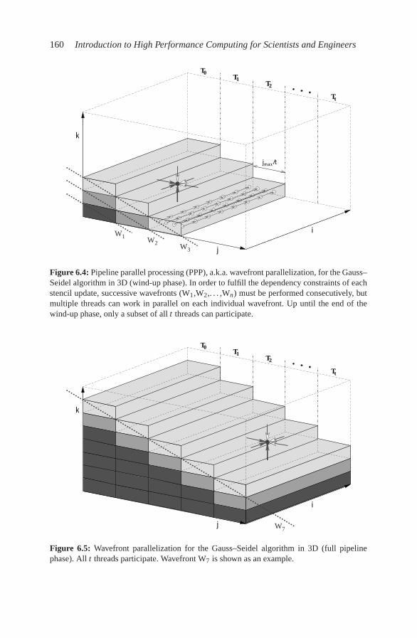
160 Introduction to High Performance Computing for Scientists and Engineers
T1T2
Tt
T0
maxj /t
12
3
i
j
k
WW
W
Figure 6.4: Pipeline parallel processing (PPP), a.k.a. wavefront parallelization, for the Gauss–Seidel algorithm in 3D (wind-up phase). In order to fulfill the dependency constraints of eachstencil update, successive wavefronts (W1,W2,. . . ,Wn) must be performed consecutively, butmultiple threads can work in parallel on each individual wavefront. Up until the end of thewind-up phase, only a subset of all t threads can participate.
T1T2
Tt
T0
i
j
k
7W
Figure 6.5: Wavefront parallelization for the Gauss–Seidel algorithm in 3D (full pipelinephase). All t threads participate. Wavefront W7 is shown as an example.

Shared-memory parallel programming with OpenMP 161
Listing 6.7: The wavefront-parallel Gauss–Seidel algorithm in three dimensions. Loop-carrieddependencies are still present, but threads can work in parallel.
1 !$OMP PARALLEL PRIVATE(k,j,i,jStart,jEnd,threadID)
2 threadID=OMP_GET_THREAD_NUM()
3 !$OMP SINGLE
4 numThreads=OMP_GET_NUM_THREADS()
5 !$OMP END SINGLE
6 jStart=jmax/numThreads*threadID
7 jEnd=jStart+jmax/numThreads ! jmax is amultiple of numThreads
8 do l=1,kmax+numThreads-1
9 k=l-threadID
10 if((k.ge.1).and.(k.le.kmax)) then
11 do j=jStart,jEnd ! this is the actual parallel loop
12 do i=1,iMax
13 phi(i,j,k) = ( phi(i-1,j,k) + phi(i+1,j,k)
14 + phi(i,j-1,k) + phi(i,j+1,k)
15 + phi(i,j,k-1) + phi(i,j,k+1) ) * osth
16 enddo
17 enddo
18 endif
19 !$OMP BARRIER
20 enddo
21 !$OMP END PARALLEL
wavefronts, and k is the current k coordinate for each thread. The OpenMP barrierin line 19 is the point where all threads (including possible idle threads) synchronizeafter a wavefront has been completed.
We have ignored possible scalar optimizations like outer loop unrolling (see theorder of site updates illustrated in the T2 block of Figure 6.4). Note that the stencilupdate is unchanged from the original version, so there are still loop-carried depen-dencies. These inhibit fully pipelined execution of the inner loop, but this may be ofminor importance if performance is bound by memory bandwidth. See Problem 6.6for an alternative solution that enables pipelining (and thus vectorization).
Wavefront methods are of utmost importance in High Performance Computing,for massively parallel applications [L76, L78] as well as for optimizing shared-memory codes [O52, O59]. Wavefronts are a natural extension of the pipeliningscheme to medium- and coarse-grained parallelism. Unfortunately, mainstream pro-gramming languages and parallelization paradigms do not as of now contain anydirect support for it. Furthermore, although dependency analysis is a major part ofthe optimization stage in any modern compiler, very few current compilers are ableto perform automatic wavefront parallelization [O59].
Note that stencil algorithms (for which Gauss–Seidel and Jacobi are just twosimple examples) are core components in a lot of simulation codes and PDE solvers.Many optimization, parallelization, and vectorization techniques have been devisedover the past decades, and there is a vast amount of literature available. More infor-mation can be found in the references [O60, O61, O62, O63].

162 Introduction to High Performance Computing for Scientists and Engineers
Problems
For solutions see page 298 ff.
6.1 OpenMP correctness. What is wrong with this OpenMP-parallel Fortran 90code?
1 double precision, dimension(0:360) :: a
2
3 !$OMP PARALLEL DO
4 do i=0,360
5 call f(dble(i)/360*PI, a(i))
6 enddo
7 !$OMP END PARALLEL DO
8
9 ...
10
11 subroutine f(arg, ret)
12 double precision :: arg, ret, noise=1.d-6
13 ret = SIN(arg) + noise
14 noise = -noise
15 return
16 end subroutine
6.2 π by Monte Carlo. The quarter circle in the first quadrant with origin at (0,0)and radius 1 has an area of π/4. Look at the random number pairs in [0,1]×[0,1]. The probability that such a point lies inside the quarter circle is π/4, sogiven enough statistics we are able to calculate π using this so-called Monte
Carlo method (see Figure 6.6). Write a parallel OpenMP program that per-forms this task. Use a suitable subroutine to get separate random number se-
Figure 6.6: Calculating π by a Monte Carlomethod (see Problem 6.2). The probabilitythat a random point in the unit square liesinside the quarter circle is π/4.
y
x1
0
1

Shared-memory parallel programming with OpenMP 163
quences for all threads. Make sure that adding more threads in a weak scalingscenario actually improves statistics.
6.3 Disentangling critical regions. In Section 6.1.4 we demonstrated the use ofnamed critical regions to prevent deadlocks. Which simple modification of theexample code would have made named the names obsolete?
6.4 Synchronization perils. What is wrong with this code?
1 !$OMP PARALLEL DO SCHEDULE(STATIC) REDUCTION(+:sum)
2 do i=1,N
3 call do_some_big_stuff(i,x)
4 sum = sum + x
5 call write_result_to_file(omp_get_thread_num(),x)
6 !$OMP BARRIER
7 enddo
8 !$OMP END PARALLEL DO
6.5 Unparallelizable? (This problem appeared on the official OpenMP mailing listin 2007.) Parallelize the loop in the following piece of code using OpenMP:
1 double precision, parameter :: up = 1.00001d0
2 double precision :: Sn
3 double precision, dimension(0:len) :: opt
4
5 Sn = 1.d0
6 do n = 0,len
7 opt(n) = Sn
8 Sn = Sn * up
9 enddo
Simply writing an OpenMP worksharing directive in front of the loop will notwork because there is a loop-carried dependency: Each iteration depends onthe result from the previous one. The parallelized code should work indepen-dently of the OpenMP schedule used. Try to avoid — as far as possible —expensive operations that might impact serial performance.
To solve this problem you may want to consider using the FIRSTPRIVATEand LASTPRIVATE OpenMP clauses. LASTPRIVATE can only be appliedto a worksharing loop construct, and has the effect that the listed variables’values are copied from the lexically last loop iteration to the global variablewhen the parallel loop exits.
6.6 Gauss–Seidel pipelined. Devise a reformulation of the Gauss–Seidel sweep(Listing 6.6) so that the inner loop does not contain loop-carried dependen-cies any more. Hint: Choose some arbitrary site from the lattice and visualizeall other sites that can be updated at the same time, obeying the dependencyconstraints. What would be the performance impact of this formulation oncache-based processors and vector processors (see Section 1.6)?

Chapter 7
Efficient OpenMP programming
OpenMP seems to be the easiest way to write parallel programs as it features a sim-ple, directive-based interface and incremental parallelization, meaning that the loopsof a program can be tackled one by one without major code restructuring. It turns out,however, that getting a truly scalable OpenMP program is a significant undertakingin all but the most trivial cases. This chapter pinpoints some of the performance prob-lems that can arise with OpenMP shared-memory programming and how they can becircumvented. We then turn to the OpenMP parallelization of the sparse MVM codethat has been introduced in Chapter 3.
There is a broad literature on viable optimizations for OpenMP programs [P12,O64]. This chapter can only cover the most relevant basics, but should suffice as astarting point.
7.1 Profiling OpenMP programs
As in serial optimization, profiling tools can often hint at the root causes for per-formance problems also with OpenMP. In the simplest case, one could employ anyof the methods described in Section 2.1 on a per-thread basis and compare the dif-ferent scalar profiles. This strategy has several drawbacks, the most important beingthat scalar tools have no concept of specific OpenMP features. In a scalar profile,OpenMP constructs like team forks, barriers, spin loops, locks, critical sections, andeven parts of user code that were packed into a separate function by the compilerappear as normal functions whose purpose can only be deduced from some more orless cryptic name.
More advanced tools allow for direct determination of load imbalance, serial frac-tion, OpenMP loop overhead, etc. (see below for more discussion regarding thoseissues). At the time of writing, very few production-grade free tools are available forOpenMP profiling, and the introduction of tasking in the OpenMP 3.0 standard hascomplicated matters for tool developers.
Figure 7.1 shows an event timeline comparison between two runs of the samecode, using Intel’s Thread Profiler for Windows [T23]. An event timeline containsinformation about the behavior of the application over time. In the case of OpenMPprofiling, this pertains to typical constructs like parallel loops, barriers, locks, andalso performance issues like load imbalance or insufficient parallelism. As a simplebenchmark we choose the multiplication of a lower triangular matrix with a vector:
165

166 Introduction to High Performance Computing for Scientists and Engineers
1 do k=1,NITER
2 !$OMP PARALLEL DO SCHEDULE(RUNTIME)
3 do row=1,N
4 do col=1,row
5 C(row) = C(row) + A(col,row) * B(col)
6 enddo
7 enddo
8 !$OMP END PARALLEL DO
9 enddo
(Note that privatizing the inner loop variable is not required here because this is au-tomatic in Fortran, but not in C/C++.) If static scheduling is used, this problem obvi-ously suffers from severe load imbalance. The bottom panel in Figure 7.1 shows thetimeline for two threads and STATIC scheduling. The lower thread (shown in black)is a “shepherd” thread that exists for administrative purposes and can be ignoredbecause it does not execute user code. Until the first parallel region is encountered,only one thread executes. After that, each thread is shown using different colors orshadings which encode the kind of activity it performs. Hatched areas denote “spin-ning,” i.e., the thread waits in a loop until given more work to do or until it hits abarrier (actually, after some time, spinning threads are often put to sleep so as tofree resources; this can be observed here just before the second barrier. This behav-ior can usually be influenced by the user). As expected, the static schedule leads tostrong load imbalance so that more than half of the first thread’s CPU time is wasted.With STATIC,16 scheduling (top panel), the imbalance is gone and performance isimproved by about 30%.
Thread profilers are usually capable of much more than just timeline displays.Often, a simple overall summary denoting, e.g., the fraction of walltime spent in bar-riers, spin loops, critical sections, or locks can reveal the nature of some performanceproblem.
7.2 Performance pitfalls
Like any other parallelization method, OpenMP is prone to the standard prob-lems of parallel programming: Serial fraction (Amdahl’s Law) and load imbalance,both discussed in Chapter 5. Communication (in terms of data transfer) is usually notmuch of an issue on shared memory as the access latencies inside a compute node aresmall and bandwidths are large (see, however, Chapter 8 for problems connected tomemory access on ccNUMA architectures). The load imbalance problem can oftenbe solved by choosing a suitable OpenMP scheduling strategy (see Section 6.1.6).However there are also very specific performance problems that are inherently con-nected to shared-memory programming in general and OpenMP in particular. In thissection we will try to give some practical advice for avoiding typical OpenMP per-formance traps.

Efficient OpenMP programming 167
Fig
ure
7.1
:(S
eeco
lor
inse
rtaf
ter
page
262.
)E
vent
tim
elin
eco
mpa
riso
nof
ath
read
edco
de(t
rian
gula
rm
atri
x-ve
ctor
mul
tipl
icat
ion)
wit
hSTATIC,16
(top
pane
l)an
dSTATIC
(bot
tom
pane
l)O
penM
Psc
hedu
ling
.

168 Introduction to High Performance Computing for Scientists and Engineers
Figure 7.2: Dual-socket dual-core Xeon 5160node used for most benchmarks in this chapter.
socket
32k L1D 32k L1D 32k L1D 32k L1D
Chipset
Memory
P P P P
4MB L2 4MB L2
7.2.1 Ameliorating the impact of OpenMP worksharing constructs
Whenever a parallel region is started or stopped or a parallel loop is initiatedor ended, there is some nonnegligible overhead involved. Threads must be spawnedor at least woken up from an idle state, the size of the work packages (chunks) foreach thread must be determined, in the case of tasking or dynamic/guided schedulingschemes each thread that becomes available must be supplied with a new task towork on, and the default barrier at the end of worksharing constructs or parallelregions synchronizes all threads. In terms of the refined scalability models discussedin Section 5.3.6, these contributions could be counted as “communication overhead.”Since they tend to be linear in the number of threads, it seems that OpenMP is notreally suited for strong scaling scenarios; with N threads, the speedup is
Somp(N) =1
s+(1− s)/N +κN +λ, (7.1)
with λ denoting N-independent overhead. For large N this expression goes to zero,which seems to be a definite showstopper for the OpenMP programming model. Inpractice, however, all is not lost: The performance impact depends on the actualvalues of κ and λ , of course. If some simple guidelines are followed, the adverseeffects of OpenMP overhead can be much reduced:
Run serial code if parallelism does not pay off
This is perhaps the most popular performance issue with OpenMP. If the work-sharing construct does not contain enough “work” per thread because, e.g., eachiteration of a short loop executes in a short time, OpenMP overhead will lead to verybad performance. It is then better to execute a serial version if the loop count is belowsome threshold. The OpenMP IF clause helps with this:
1 !$OMP PARALLEL DO IF(N>1700)
2 do i=1,N
3 A(i) = B(i) + C(i) * D(i)
4 enddo
5 !$OMP END PARALLEL DO

Efficient OpenMP programming 169
101
102
103
104
105
106
N
0
1000
2000
3000
4000
5000M
Flo
ps/s
ec
serial1 thread4 threads4 threads, IF(N>1700)
Figure 7.3: OpenMP overhead and the benefits of the IF(N>1700) clause for the vectortriad benchmark. (Dual-socket dual-core Intel Xeon 5160 3.0 GHz system like in Figure 7.2,Intel compiler 10.1).
Figure 7.3 shows a comparison of vector triad data in the purely serial case andwith one and four OpenMP threads, respectively, on a dual-socket Xeon 5160 node(sketched in Figure 7.2). The presence of OpenMP causes overhead at small N evenif only a single thread is used (see below for more discussion regarding the costof worksharing constructs). Using the IF clause leads to an optimal combinationof threaded and serial loop versions if the threshold is chosen appropriately, and ishence mandatory when large loop lengths cannot be guaranteed. However, at N .
1000 there is still some measurable performance hit; after all, more code must beexecuted than in the purely serial case. Note that the IF clause is a (partial) cure forthe symptoms, but not the reasons for parallel loop overhead. The following sectionswill elaborate on methods that can actually reduce it.
Instead of disabling parallel execution altogether, it may also be an option toreduce the number of threads used on a particular parallel region by means of theNUM_THREADS clause:
1 !$OMP PARALLEL DO NUM_THREADS(2)
2 do i=1,N
3 A(i) = B(i) + C(i) * D(i)
4 enddo
5 !$OMP END PARALLEL DO
Fewer threads mean less overhead, and the resulting performance may be better thanwith IF, at least for some loop lengths.

170 Introduction to High Performance Computing for Scientists and Engineers
Avoid implicit barriers
Be aware that most OpenMP worksharing constructs (including OMP DO/ENDDO) insert automatic barriers at the end. This is the safe default, so that all threadshave completed their share of work before anything after the construct is executed.In cases where this is not required, a NOWAIT clause removes the implicit barrier:
1 !$OMP PARALLEL
2 !$OMP DO
3 do i=1,N
4 A(i) = func1(B(i))
5 enddo
6 !$OMP END DO NOWAIT
7 ! still in parallel region here. do more work:
8 !$OMP CRITICAL
9 CNT = CNT + 1
10 !$OMP END CRITICAL
11 !$OMP END PARALLEL
There is also an implicit barrier at the end of a parallel region that cannot be removed.Implicit barriers add to synchronization overhead like critical regions, but they are of-ten required to protect from race conditions. The programmer should check carefullywhether the NOWAIT clause is really safe.
Section 7.2.2 below will show how barrier overhead for the standard case of aworksharing loop can be determined experimentally.
Try to minimize the number of parallel regions
This is often formulated as the need to parallelize loop nests on a level as far outas possible, and it is inherently connected to the previous guidelines. Parallelizinginner loop levels leads to increased OpenMP overhead because a team of threads isspawned or woken up multiple times:
1 double precision :: R
2 R = 0.d0
3 do j=1,N
4 !$OMP PARALLEL DO REDUCTION(+:R)
5 do i=1,N
6 R = R + A(i,j) * B(i)
7 enddo
8 !$OMP END PARALLEL DO
9 C(j) = C(j) + R
10 enddo
In this particular example, the team of threads is restarted N times, once in each iter-ation of the j loop. Pulling the complete parallel construct to the outer loop reducesthe number of restarts to one and has the additional benefit that the reductionclause becomes obsolete as all threads work on disjoint parts of the result vector:
1 !$OMP PARALLEL DO
2 do j=1,N
3 do i=1,N

Efficient OpenMP programming 171
4 C(j) = C(j) + A(i,j) * B(i)
5 enddo
6 enddo
7 !$OMP END PARALLEL DO
The less often the team of threads needs to be forked or restarted, the less over-head is incurred. This strategy may require some extra programming care because ifthe team continues running between worksharing constructs, code which would oth-erwise be executed by a single thread will be run by all threads redundantly. Considerthe following example:
1 double precision :: R,S
2 R = 0.d0
3 !$OMP PARALLEL DO REDUCTION(+:R)
4 do i=1,N
5 A(i) = DO_WORK(B(i))
6 R = R + B(i)
7 enddo
8 !$OMP END PARALLEL DO
9 S = SIN(R)
10 !$OMP PARALLEL DO
11 do i=1,N
12 A(i) = A(i) + S
13 enddo
14 !$OMP END PARALLEL DO
The SIN function call between the loops is performed by the master thread only. Atthe end of the first loop, all threads synchronize and are possibly even put to sleep,and they are started again when the second loop executes. In order to circumvent thisoverhead, a continuous parallel region can be employed:
1 double precision :: R,S
2 R = 0.d0
3 !$OMP PARALLEL PRIVATE(S)
4 !$OMP DO REDUCTION(+:R)
5 do i=1,N
6 A(i) = DO_WORK(B(i))
7 R = R + B(i)
8 enddo
9 !$OMP END DO
10 S = SIN(R)
11 !$OMP DO
12 do i=1,N
13 A(i) = A(i) + S
14 enddo
15 !$OMP END DO NOWAIT
16 !$OMP END PARALLEL
Now the SIN function in line 10 is computed by all threads, and consequently S
must be privatized. It is safe to use the NOWAIT clause on the second loop in orderto reduce barrier overhead. This is not possible with the first loop as the final resultof the reduction will only be valid after synchronization.

172 Introduction to High Performance Computing for Scientists and Engineers
Avoid “trivial” load imbalance
The number of tasks, or the parallel loop trip count, should be large compared tothe number of threads. If the trip count is a small noninteger multiple of the numberof threads, some threads will end up doing significantly less work than others, leadingto load imbalance. This effect is independent of any other load balancing or overheadissues, i.e., it occurs even if each task comprises exactly the same amount of work,and also if OpenMP overhead is negligible.
A typical situation where it may become important is the execution of deep loopnests on highly threaded architectures [O65] (see Section 1.5 for more informationon hardware threading). The larger the number of threads, the fewer tasks per threadare available on the parallel (outer) loop:
1 double precision, dimension(N,N,N,M) :: A
2 !$OMP PARALLEL DO SCHEDULE(STATIC) REDUCTION(+:res)
3 do l=1,M
4 do k=1,N
5 do j=1,N
6 do i=1,N
7 res = res + A(i,j,k,l)
8 enddo ; enddo ; enddo ; enddo
9 !$OMP END PARALLEL DO
The outer loop is the natural candidate for parallelization here, causing the minimalnumber of executed worksharing loops (and implicit barriers) and generating theleast overhead. However, the outer loop length M may be quite small. Under the bestpossible conditions, if t is the number of threads, t −mod(M, t) threads receive achunk that is one iteration smaller than for the other threads. If M/t is small, loadimbalance will hurt scalability.
The COLLAPSE clause (introduced with OpenMP 3.0) can help here. For perfect
loop nests, i.e., with no code between the different do (and enddo) statements andloop counts not depending on each other, the clause collapses a specified number ofloop levels into one. Computing the original loop indices is taken care of automati-cally, so that the loop body can be left unchanged:
1 double precision, dimension(N,N,N,M) :: A
2 !$OMP PARALLEL DO SCHEDULE(STATIC) REDUCTION(+:res) COLLAPSE(2)
3 do l=1,M
4 do k=1,N
5 do j=1,N
6 do i=1,N
7 res = res + A(i,j,k,l)
8 enddo ; enddo ; enddo ; enddo
9 !$OMP END PARALLEL DO
Here the outer two loop levels are collapsed into one with a loop length of M×N, andthe resulting long loop will be executed by all threads in parallel. This amelioratesthe load balancing problem.

Efficient OpenMP programming 173
1 2 4 8 16 32 64Chunksize
0
5
10
15
20
25P
erf
orm
an
ce
[M
Ite
ratio
ns/s
]
1S dynamic
1S static
1S guided
2S dynamic
2S static
2S guided 1 4 16 640
100
200
300
400
Ove
rhe
ad
[cycle
s]
1S dynamic
2S dynamic
2S static
static baseline
Figure 7.4: Main panel: Performance of a trivial worksharing loop with a large loop countunder static (filled circles) versus dynamic (open symbols) scheduling on two cores in an L2group (1S) or on different sockets (2S) of a dual-socket dual-core Intel Xeon 5160 3.0 GHzsystem like in Figure 7.2 (Intel Compiler 10.1). Inset: Overhead in processor cycles for as-signing a single chunk to a thread.
Avoid dynamic/guided loop scheduling or tasking unless necessary
All parallel loop scheduling options (except STATIC) and tasking constructsrequire some amount of nontrivial computation or bookkeeping in order to figure outwhich thread is to compute the next chunk or task. This overhead can be significantif each task contains only a small amount of work. One can get a rough estimate forthe cost of assigning a new loop chunk to a thread with a simple benchmark test.Figure 7.4 shows a performance comparison between static and dynamic schedulingfor a simple parallel loop with purely computational workload:
1 !$OMP PARALLEL DO SCHEDULE(RUNTIME) REDUCTION(+:s)
2 do i=1,N
3 s = s + compute(i)
4 enddo
5 !$OMP END PARALLEL DO
The compute() function performs some in-register calculations (like, e.g., tran-scendental function evaluations) for some hundreds of cycles. It is unimportant whatit does exactly, as long as it neither interferes with the main parallel loop nor incursbandwidth bottlenecks on any memory level. N should be chosen large enough so that

174 Introduction to High Performance Computing for Scientists and Engineers
OpenMP loop startup overhead becomes negligible. The performance baseline witht threads, Ps(t), is then measured with static scheduling without a chunksize, in unitsof million iterations per second (see the dotted line in Figure 7.4 for two threads ontwo cores of the Xeon 5160 dual-core dual-socket node depicted in Figure 7.2). Thisbaseline does not depend on the binding of the threads to cores (inside cache groups,across ccNUMA domains, etc.) because each thread executes only a single chunk,and any OpenMP overhead occurs only at the start and at the end of the worksharingconstruct. At large N, the static baseline should thus be t times larger than the purelyserial performance.
Whenever a chunksize is used with any scheduling variant, assigning a new chunkto a thread will take some time, which counts as overhead. The main panel in Fig-ure 7.4 shows performance data for static (circles), dynamic (squares), and guided(diamonds) scheduling when the threads run in an L2 cache group (closed sym-bols) or on different sockets (open symbols), respectively. As expected, the over-head is largest for small chunks, and dominant only for dynamic scheduling. Guidedscheduling performs best because larger chunks are assigned at the beginning of theloop, and the indicated chunksize is just a lower bound (see Figure 6.2). The dif-ference between intersocket and intra-L2 situations is only significant with dynamicscheduling, because some common resource is required to arbitrate work distribu-tion. If this resource can be kept in a shared cache, chunk assignment will be muchfaster. It will also be faster with guided scheduling, but due to the large average
chunksize, the effect is unnoticeable.If P(t,c) is the t-thread performance at chunksize c, the difference in per-iteration
per-thread execution times between the static baseline and the “chunked” version isthe per-iteration overhead. Per complete chunk, this is
To(t,c) =t
c
(
1P(t,c)
− 1Ps(t)
)
. (7.2)
The inset in Figure 7.4 shows that the overhead in CPU cycles is roughly independentof chunksize, at least for chunks larger than 4. Assigning a new chunk to a threadcosts over 200 cycles if both threads run inside an L2 group, and 350 cycles whenrunning on different sockets (these times include the 50 cycle penalty per chunk forstatic scheduling). Again we encounter a situation where mutual thread placement,or affinity, is decisive.
Please note that, although the general methodology is applicable to all shared-memory systems, the results of this analysis depend on hardware properties and theactual implementation of OpenMP worksharing done by the compiler. The actualnumbers may differ significantly on other platforms.
Other factors not recognized by this benchmark can impact the performance ofdynamically scheduled worksharing constructs. In memory-bound loop code, pre-fetching may be inefficient or impossible if the chunksize is small. Moreover, due tothe indeterministic nature of memory accesses, ccNUMA locality could be hard tomaintain, which pertains to guided scheduling as well. See Section 8.3.1 for detailson this problem.

Efficient OpenMP programming 175
7.2.2 Determining OpenMP overhead for short loops
The question arises how one can estimate the possible overheads that go alongwith a parallel worksharing construct. In general, the overhead consists of a constantpart and a part that depends on the number of threads. There are vast differencesfrom system to system as to how large it can be, but it is usually of the order of atleast hundreds if not thousands of CPU cycles. It can be determined easily by fittinga simple performance model to data obtained from a low-level benchmark. As anexample we pick the vector triad with short vector lengths and static scheduling sothat the parallel run scales across threads if each core has its own L1 (performancewould not scale with larger vectors as shared caches or main memory usually presentbottlenecks, especially on multicore systems):
1 !$OMP PARALLEL PRIVATE(j)
2 do j=1,NITER
3 !$OMP DO SCHEDULE(static) NOWAIT ! nowait is optional (see text)
4 do i=1,N
5 A(i) = B(i) + C(i) * D(i)
6 enddo
7 !$OMP END DO
8 enddo
9 !$OMP END PARALLEL
As usual, NITER is chosen so that overall runtime can be accurately measured andone-time startup effects (loading data into cache the first time etc.) become unimpor-tant. The NOWAIT clause is optional and is used here only to demonstrate the impactof the implied barrier at the end of the loop worksharing construct (see below).
The performance model assumes that overall runtime with a problem size of N
on t threads can be split into computational and setup/shutdown contributions:
T (N, t) = Tc(N, t)+Ts(t) . (7.3)
Further assuming that we have measured purely serial performance Ps(N) we canwrite
Tc(N, t) =2N
tPs(N/t), (7.4)
which allows an N-dependent performance behavior unconnected to OpenMP over-head. The factor of two in the numerator accounts for the fact that performance ismeasured in MFlops/sec and each loop iteration comprises two Flops. As mentionedabove, setup/shutdown time is composed of a constant latency and a component thatdepends on the number of threads:
Ts(t) = Tl +Tp(t) . (7.5)
Now we can calculate parallel performance on t threads at problem size N:
P(N, t) =2N
T (N, t)=
2N
2N [tPs(N/t)]−1 +Ts(t)(7.6)

176 Introduction to High Performance Computing for Scientists and Engineers
Figure 7.5 shows performance data for the small-N vector triad on a node with fourcores (two sockets), including parametric fits to the model (7.6) for the one- (circles)and four-thread (squares) cases, and with the implied barrier removed (open symbols)by a nowait clause. The indicated fit parameters in nanoseconds denote Ts(t), asdefined in (7.5). The values measured for Ps with the serial code version are not useddirectly for fitting but approximated by
Ps(N) =2N
2N/Pmax +T0, (7.7)
where Pmax is the asymptotic serial triad performance and T0 summarizes all thescalar overhead (pipeline startup, loop branch misprediction, etc.). Both parametersare determined by fitting to measured serial performance data (dotted-dashed line inFigure 7.5). Then, (7.7) is used in (7.6):
P(N, t) =1
(tPmax)−1 +(T0 +Ts(t))/2N(7.8)
Surprisingly, there is a measurable overhead for running with a single OpenMPthread versus purely serial mode. However, as the two versions reach the same as-ymptotic performance at N . 1000, this effect cannot be attributed to inefficientscalar code, although OpenMP does sometimes prevent advanced loop optimizations.The single-thread overhead originates from the inability of the compiler to generatea separate code version for serial execution.
The barrier is negligible with a single thread, and accounts for most of the over-head at four threads. But even without it about 190 ns (570 CPU cycles) are spent forsetting up the worksharing loop in that case (one could indeed estimate the averagememory latency from the barrier overhead, assuming that the barrier is implementedby a memory variable which must be updated by all threads in turn). The data labeled“restart” (diamonds) was obtained by using a combined parallel do directive,so that the team of threads is woken up each time the inner loop gets executed:
1 do j=1,NITER
2 !$OMP PARALLEL DO SCHEDULE(static)
3 do i=1,N
4 A(i) = B(i) + C(i) * D(i)
5 enddo
6 !$OMP END PARALLEL DO
7 enddo
This makes it possible to separate the thread wakeup time from the barrier and work-sharing overheads: There is an additional cost of nearly 460 ns (1380 cycles) forrestarting the team, which proves that it can indeed be beneficial to minimize thenumber of parallel regions in an OpenMP program, as mentioned above.
Similar to the experiments performed with dynamic scheduling in the previoussection, the actual overhead incurred for small OpenMP loops depends on many fac-tors like the compiler and runtime libraries, organization of caches, and the generalnode structure. It also makes a significant difference whether the thread team resides

Efficient OpenMP programming 177
10 100 1000N
0
1000
2000
3000
4000P
erf
orm
ance [M
Flo
ps/s
ec]
serialserial fit4 threads restart4 threads4 threads nowait1 thread1 thread nowait
880 ns
190 ns
20 ns
12 ns
1340 ns
Figure 7.5: OpenMP loop overhead Ts(t) for the small-N vector triad, determined from fittingthe model (7.6) to measured performance data. Note the large impact of the implied barrier(removed by the nowait clause). The diamonds indicate data obtained by restarting the par-allel region on every triad loop. (Intel Xeon 5160 3.0 GHz dual-core dual-socket node (seeFigure 7.2), Intel Compiler 10.1.)
inside a cache group or encompasses several groups [M41] (see Appendix A for in-formation on how to use affinity mechanisms). It is a general result, however, thatimplicit (and explicit) barriers are the largest contributors to OpenMP-specific paral-lel overhead. The EPCC OpenMP microbenchmark suite [136] provides a frameworkfor measuring many OpenMP-related timings, including barriers, but use an approachslightly different from the one shown here.
7.2.3 Serialization
The most straightforward way to coordinate access to shared resources is to usecritical region. Unless used with caution, these bear the potential of serializing thecode. In the following example, columns of the matrix M are updated in parallel.Which columns get updated is determined by the col_calc() function:
1 double precision, dimension(N,N) :: M
2 integer :: c
3 ...
4 !$OMP PARALLEL DO PRIVATE(c)
5 do i=1,K
6 c = col_calc(i)
7 !$OMP CRITICAL
8 M(:,c) = M(:,c) + f(c)

178 Introduction to High Performance Computing for Scientists and Engineers
9 !$OMP END CRITICAL
10 enddo
11 !$OMP END PARALLEL DO
Function f() returns an array, which is added to column c of the matrix. Since it ispossible that a column is updated more than once, the array summation is protectedby a critical region. However, if most of the CPU time is spent in line 8, the programis effectively serialized and there will be no gain from using more than one thread;the program will even run slower because of the additional overhead for entering acritical construct.
This coarse-grained way of protecting a resource (matrix M in this case) is oftencalled a big fat lock. One solution could be to make use of the resource’s substructure,i.e., the property of the matrix to consist of individual columns, and protect accessto each column separately. Serialization can then only occur if two threads try toupdate the same column at the same time. Unfortunately, named critical regions (seeSection 6.1.4) are of no use here as the name cannot be a variable. However, it ispossible to use a separate OpenMP lock variable for each column:
1 double precision, dimension(N,N) :: M
2 integer (kind=omp_lock_kind), dimension(N) :: locks
3 integer :: c
4 !$OMP PARALLEL
5 !$OMP DO
6 do i=1,N
7 call omp_init_lock(locks(i))
8 enddo
9 !$OMP END DO
10 ...
11 !$OMP DO PRIVATE(c)
12 do i=1,K
13 c = col_calc(i)
14 call omp_set_lock(locks(c))
15 M(:,c) = M(:,c) + f(c)
16 call omp_unset_lock(locks(c))
17 enddo
18 !$OMP END DO
19 !$OMP END PARALLEL
If the mapping of i to c, mediated by the col_calc() function, is such that notonly a few columns get updated, parallelism is greatly enhanced by this optimization(see [A83] for a real-world example). One should be aware though that setting andunsetting OpenMP locks incurs some overhead, as is the case for entering and leavinga critical region. If this overhead is comparable to the cost for updating a matrix row,the fine-grained synchronization scheme is of no use.
There is a solution to this problem if memory is not a scarce resource: One mayuse thread-local copies of otherwise shared data that get “pulled together” by, e.g.,a reduction operation at the end of a parallel region. In our example this can beachieved most easily by doing an OpenMP reduction on M. If K is large enough, theadditional cost is negligible:

Efficient OpenMP programming 179
1 double precision, dimension(1:N,1,N) :: M
2 integer :: c
3 ...
4 !$OMP PARALLEL DO PRIVATE(c) REDUCTION(+:M)
5 do i=1,K
6 c = col_calc(i)
7 M(:,c) = M(:,c) + f(c)
8 enddo
9 !$OMP END PARALLEL DO
Note that reductions on arrays are only allowed in Fortran, and some further restric-tions apply [P11]. In C/C++ it would be necessary to perform explicit privatizationinside the parallel region (probably using heap memory) and do the reduction manu-ally, as shown in Listing 6.2.
In general, privatization should be given priority over synchronization when pos-sible. This may require a careful analysis of the costs involved in the needed copyingand reduction operations.
7.2.4 False sharing
The hardware-based cache coherence mechanisms described in Section 4.2.1make the use of caches in a shared-memory system transparent to the programmer.In some cases, however, cache coherence traffic can throttle performance to very lowlevels. This happens if the same cache line is modified continuously by a group ofthreads so that the cache coherence logic is forced to evict and reload it in rapidsuccession. As an example, consider a program fragment that calculates a histogramover the values in some large integer array A that are all in the range {1, . . . ,8}:
1 integer, dimension(8) :: S
2 integer :: IND
3 S = 0
4 do i=1,N
5 IND = A(i)
6 S(IND) = S(IND) + 1
7 enddo
In a straightforward parallelization attempt one would probably go about and makeS two-dimensional, reserving space for the local histogram of each thread in order toavoid serialization on the shared resource, array S:
1 integer, dimension(:,:), allocatable :: S
2 integer :: IND,ID,NT
3 !$OMP PARALLEL PRIVATE(ID,IND)
4 !$OMP SINGLE
5 NT = omp_get_num_threads()
6 allocate(S(0:NT,8))
7 S = 0
8 !$OMP END SINGLE
9 ID = omp_get_thread_num() + 1
10 !$OMP DO
11 do i=1,N

180 Introduction to High Performance Computing for Scientists and Engineers
12 IND = A(i)
13 S(ID,IND) = S(ID,IND) + 1
14 enddo
15 !$OMP END DO NOWAIT
16 ! calculate complete histogram
17 !$OMP CRITICAL
18 do j=1,8
19 S(0,j) = S(0,j) + S(ID,j)
20 enddo
21 !$OMP END CRITICAL
22 !$OMP END PARALLEL
The loop starting at line 18 collects the partial results of all threads. Although this is avalid OpenMP program, it will not run faster but much more slowly when using fourthreads instead of one. The reason is that the two-dimensional array S contains all thehistogram data from all threads. With four threads these are 160 bytes, correspondingto two or three cache lines on most processors. On each histogram update to S inline 13, the writing CPU must gain exclusive ownership of one of those cache lines;almost every write leads to a cache miss and subsequent coherence traffic because itis likely that the needed cache line resides in another processor’s cache, in modifiedstate. Compared to the serial case where S fits into the cache of a single CPU, thiswill result in disastrous performance.
One should add that false sharing can be eliminated in simple cases by the stan-dard register optimizations of the compiler. If the crucial update operation can beperformed to a register whose contents are only written out at the end of the loop, nowrite misses turn up. This is not possible in the above example, however, because ofthe computed second index to S in line 13.
Getting rid of false sharing by manual optimization is often a simple task once theproblem has been identified. A standard technique is array padding, i.e., insertion ofa suitable amount of space between memory locations that get updated by differentthreads. In the histogram example above, allocating S in line 6 as S(0:NT*CL,8),with CL being the cache line size in integers, will reserve an exclusive cache linefor each thread. Of course, the first index to S will have to be multiplied by CL
everywhere else in the program (transposing S will save some memory, but the mainprinciple stays the same).
An even more painless solution exists in the form of data privatization (see alsoSection 7.2.3 above): On entry to the parallel region, each thread gets its own localcopy of the histogram array in its own stack space. It is very unlikely that thosedifferent instances will occupy the same cache line, so false sharing is not a problem.Moreover, the code is simplified and made equivalent to the purely serial version byusing the REDUCTION clause:
1 integer, dimension(8) :: S
2 integer :: IND
3 S=0
4 !$OMP PARALLEL DO PRIVATE(IND) REDUCTION(+:S)
5 do i=1,N
6 IND = A(i)
7 S(IND) = S(IND) + 1

Efficient OpenMP programming 181
T0
T1
T2
T3
T4
+= *
Figure 7.6: Parallelization approach for sparse MVM (five threads). All marked elements arehandled in a single iteration of the parallelized loop. The RHS vector is accessed by all threads.
8 enddo
9 !$OMP EMD PARALLEL DO
Setting S to zero is only required if the code is to be compiled without OpenMPsupport, as the reduction clause automatically initializes the variables in questionwith appropriate starting values.
Again, privatization in its most convenient form (reduction) is possible here be-cause we are using Fortran (the OpenMP standard allows no reductions on arrays inC/C++) and the elementary operation (addition) is supported for the REDUCTIONclause. However, even without the clause the required operations are easy to formu-late explicitly (see Problem 7.1).
7.3 Case study: Parallel sparse matrix-vector multiply
As an interesting application of OpenMP to a nontrivial problem we now extendthe considerations on sparse MVM data layout and optimization by parallelizing theCRS and JDS matrix-vector multiplication codes from Section 3.6 [A84, A82].
No matter which of the two storage formats is chosen, the general parallelizationapproach is always the same: In both cases there is a parallelizable loop that calcu-lates successive elements (or blocks of elements) of the result vector (see Figure 7.6).For the CRS matrix format, this principle can be applied in a straightforward manner:
1 !$OMP PARALLEL DO PRIVATE(j)1
2 do i = 1,Nr
1The privatization of inner loop indices in the lexical extent of a parallel outer loop is not strictlyrequired in Fortran, but it is in C/C++ [P11].

182 Introduction to High Performance Computing for Scientists and Engineers
3 do j = row_ptr(i), row_ptr(i+1) - 1
4 C(i) = C(i) + val(j) * B(col_idx(j))
5 enddo
6 enddo
7 !$OMP END PARALLEL DO
Due to the long outer loop, OpenMP overhead is usually not a problem here. Depend-ing on the concrete form of the matrix, however, some load imbalance might occur ifvery short or very long matrix rows are clustered at some regions. A different kind ofOpenMP scheduling strategy like DYNAMIC or GUIDED might help in this situation.
The vanilla JDS sMVM is also parallelized easily:
1 !$OMP PARALLEL PRIVATE(diag,diagLen,offset)
2 do diag=1, Nj3 diagLen = jd_ptr(diag+1) - jd_ptr(diag)
4 offset = jd_ptr(diag) - 1
5 !$OMP DO
6 do i=1, diagLen
7 C(i) = C(i) + val(offset+i) * B(col_idx(offset+i))
8 enddo
9 !$OMP END DO
10 enddo
11 !$OMP END PARALLEL
The parallel loop is the inner loop in this case, but there is no OpenMP overheadproblem as the loop count is large. Moreover, in contrast to the parallel CRS version,there is no load imbalance because all inner loop iterations contain the same amountof work. All this would look like an ideal situation were it not for the bad codebalance of vanilla JDS sMVM. However, the unrolled and blocked versions can beequally well parallelized. For the blocked code (see Figure 3.19), the outer loop overall blocks is a natural candidate:
1 !$OMP PARALLEL DO PRIVATE(block_start,block_end,i,diag,
2 !$OMP& diagLen,offset)
3 do ib=1,Nr,b
4 block_start = ib
5 block_end = min(ib+b-1,Nr)
6 do diag=1,Nj7 diagLen = jd_ptr(diag+1)-jd_ptr(diag)
8 offset = jd_ptr(diag) - 1
9 if(diagLen .ge. block_start) then
10 do i=block_start, min(block_end,diagLen)
11 C(i) = C(i)+val(offset+i)*B(col_idx(offset+i))
12 enddo
13 endif
14 enddo
15 enddo
16 !$OMP END PARALLEL DO
This version has even got less OpenMP overhead because the DO directive is onthe outermost loop. Unfortunately, there is even more potential for load imbalancebecause of the matrix rows being sorted for size. But as the dependence of workload

Efficient OpenMP programming 183
1 2 3 4# Sockets/Nodes
0
100
200
300
400
500
600
700
800M
Flo
ps/s
ec
CRS - AMD Opteron
bJDS - AMD Opteron
CRS - SGI AltixbJDS - SGI AltixCRS - Intel Xeon/Core2bJDS - Intel Xeon/Core2
1 2# Cores
0
200
400
600
Figure 7.7: Performance and strong scaling for straightforward OpenMP parallelization ofsparse MVM on three different architectures, comparing CRS (hatched bars) and blocked JDS(solid bars) variants. The Intel Xeon/Core2 system is of UMA type, the other two systemsare ccNUMA. The different scaling baselines have been separated (one socket/LD in the mainframe, one core in the inset).
on loop index is roughly predictable, a static schedule with a chunksize of one canremedy most of this effect.
Figure 7.7 shows performance and scaling behavior of the parallel CRS andblocked JDS versions on three different architectures: Two ccNUMA systems (Op-teron and SGI Altix, equivalent to the block diagrams in Figures 4.5 and 4.6), andone UMA system (Xeon/Core2 node like in Figure 4.4). In all cases, the code wasrun on as few locality domains or sockets as possible, i.e., first filling one LD orsocket before going to the next. The inset displays intra-LD or intrasocket scalabilitywith respect to the single-core scaling baseline. All systems considered are stronglybandwidth-limited on this level. The performance gain from using a second threadis usually far from a factor of two, as may be expected. Note, however, that this be-havior also depends crucially on the ability of one core to utilize the local memoryinterface: The relatively low single-thread CRS performance on the Altix leads to asignificant speedup of approximately 1.8 for two threads (see also Section 5.3.8).
Scalability across sockets or LDs (main frame in Figure 7.7) reveals a crucialdifference between ccNUMA and UMA systems. Only the UMA node shows theexpected speedup when the second socket gets used, due to the additional bandwidthprovided by the second frontside bus (it is a known problem of FSB-based designsthat bandwidth scalability across sockets is less than perfect, so we don’t see a fac-

184 Introduction to High Performance Computing for Scientists and Engineers
tor of two here). Although ccNUMA architectures should be able to deliver scalablebandwidth, both code versions seem to be extremely unsuitable for ccNUMA, ex-hibiting poor scalability or, in case of the Altix, even performance breakdowns atlarger numbers of LDs.
The reason for the failure of ccNUMA to deliver the expected bandwidth lies inour ignorance of a necessary prerequisite for scalability that we have not honored yet:Correct data and thread placement for access locality. See Chapter 8 for programmingtechniques that can mitigate this problem, and [O66] for a more general assessmentof parallel sparse MVM optimization on modern shared-memory systems.
Problems
For solutions see page 301 ff.
7.1 Privatization gymnastics. In Section 7.2.4 we have optimized a code for paral-lel histogram calculation by eliminating false sharing. The final code employsa REDUCTION clause to sum up all the partial results for S(). How would thecode look like in C or C++?
7.2 Superlinear speedup. When the number of threads is increased at constantproblem size (strong scaling), making additional cache space available to theapplication, there is a chance that the whole working set fits into the aggre-gated cache of all used cores. The speedup will then be larger than what theadditional number of cores seem to allow. Can you identify this situation inthe performance data for the 2D parallel Jacobi solver (Figure 6.3)? Of course,this result may be valid only for one special type of machine. What conditionmust hold for a general cache-based machine so that there is at least a chanceto see superlinear speedup with this code?
7.3 Reductions and initial values. In some of the examples for decreasing the num-ber of parallel regions on page 170 we have explicitly set the reduction variableR to zero before entering the parallel region, although OpenMP initializes suchvariables on its own. Why is it necessary then to do it anyway?
7.4 Optimal thread count. What is the optimal thread count to use for a memory-bound multithreaded application on a two-socket ccNUMA system with sixcores per socket and a three-core L3 group?

Chapter 8
Locality optimizations on ccNUMAarchitectures
It was mentioned already in the section on ccNUMA architecture that, for applica-tions whose performance is bound by memory bandwidth, locality and contentionproblems (see Figures 8.1 and 8.2) tend to turn up when threads/processes and theirdata are not carefully placed across the locality domains of a ccNUMA system. Un-fortunately, the current OpenMP standard (3.0) does not refer to page placement atall and it is up to the programmer to use the tools that system builders provide. Thischapter discusses the general, i.e., mostly system-independent options for correctdata placement, and possible pitfalls that may prevent it. We will also show that pageplacement is not an issue that is restricted to shared-memory parallel programming.
8.1 Locality of access on ccNUMA
Although ccNUMA architectures are ubiquitous today, the need for ccNUMA-awareness has not yet arrived in all application areas; memory-bound code must bedesigned to employ proper page placement [O67]. The placement problem has twodimensions: First, one has to make sure that memory gets mapped into the local-ity domains of processors that actually access them. This minimizes NUMA traffic
Memory Memory
P P P P
Figure 8.1: Locality problem on a cc-NUMA system. Memory pages got mappedinto a locality domain that is not con-nected to the accessing processor, leadingto NUMA traffic.
Memory Memory
P P P P
Figure 8.2: Contention problem on a cc-NUMA system. Even if the network is veryfast, a single locality domain can usuallynot saturate the bandwidth demands fromconcurrent local and nonlocal accesses.
185

186 Introduction to High Performance Computing for Scientists and Engineers
Figure 8.3: A ccNUMA system (based ondual-core AMD Opteron processors) withfour locality domains LD0 . . . LD3 and twocores per LD, coupled via a HyperTransportnetwork. There are three NUMA access lev-els (local domain, one hop, two hops).
LD
0
LD
1
LD
2
LD
3
HT
HT
HT HT
MI
Memory Memory
Memory Memory
P P P P
PPPP
across the network. In this context, “mapping” means that a page table entry is setup, which describes the association of a physical with a virtual memory page. Con-sequently, locality of access in ccNUMA systems is always followed on the OS pagelevel, with typical page sizes of (commonly) 4 kB or (more rarely) 16 kB, sometimeslarger. Hence, strict locality may be hard to implement with working sets that onlyencompass a few pages, although the problem tends to be cache-bound in this caseanyway. Second, threads or processes must be pinned to those CPUs which had orig-inally mapped their memory regions in order not to lose locality of access. In thefollowing we assume that appropriate affinity mechanisms have been employed (seeAppendix A).
A typical ccNUMA node with four locality domains is depicted in Figure 8.3. Ituses two HyperTransport (HT) links per socket to connect to neighboring domains,which results in a “closed chain” topology. Memory access is hence categorized intothree levels, depending on how many HT hops (zero, one, or two) are required toreach the desired page. The actual remote bandwidth and latency penalties can varysignificantly across different systems; vector triad measurements can at least providerough guidelines. See the following sections for details about how to control pageplacement.
Note that even with an extremely fast NUMA interconnect whose bandwidth andlatency are comparable to local memory access, the contention problem cannot beeliminated. No interconnect, no matter how fast, can turn ccNUMA into UMA.
8.1.1 Page placement by first touch
Fortunately, the initial mapping requirement can be fulfilled in a portable man-ner on all current ccNUMA architectures. If configured correctly (this pertains tofirmware [“BIOS”], operating system and runtime libraries alike), they support afirst touch policy for memory pages: A page gets mapped into the locality domainof the processor that first writes to it. Merely allocating memory is not sufficient.

Locality optimizations on ccNUMA architectures 187
It is therefore the data initialization code that deserves attention on ccNUMA (andusing calloc() in C will most probably be counterproductive). As an examplewe look again at a naïve OpenMP-parallel implementation of the vector triad codefrom Listing 1.1. Instead of allocating arrays on the stack, however, we now use dy-namic (heap) memory for reasons which will be explained later (we omit the timingfunctionality for brevity):
1 double precision, allocatable, dimension(:) :: A, B, C, D
2 allocate(A(N), B(N), C(N), D(N))
3 ! initialization
4 do i=1,N
5 B(i) = i; C(i) = mod(i,5); D(i) = mod(i,10)
6 enddo
7 ...
8 do j=1,R
9 !$OMP PARALLEL DO
10 do i=1,N
11 A(i) = B(i) + C(i) * D(i)
12 enddo
13 !$OMP END PARALLEL DO
14 call dummy(A,B,C,D)
15 enddo
Here we have explicitly written out the loop which initializes arrays B, C, and D withsensible data (it is not required to initialize A because it will not be read before be-ing written later). If this code, which is prototypical for many OpenMP applicationsthat have not been optimized for ccNUMA, is run across several locality domains,it will not scale beyond the maximum performance achievable on a single LD if theworking set does not fit into cache. This is because the initialization loop is executedby a single thread, writing to B, C, and D for the first time. Hence, all memory pagesbelonging to those arrays will be mapped into a single LD. As Figure 8.4 shows, theconsequences are significant: If the working set fits into the aggregated cache, scala-bility is good. For large arrays, however, 8-thread performance (filled circles) dropseven below the 2-thread (one LD) value (open diamonds), because all threads accessmemory in LD0 via the HT network, leading to severe contention. As mentionedabove, this problem can be solved by performing array initialization in parallel. Theloop from lines 4–6 in the code above should thus be replaced by:
1 ! initialization
2 !$OMP PARALLEL DO
3 do i=1,N
4 B(i) = i; C(i) = mod(i,5); D(i) = mod(i,10)
5 enddo
6 !$OMP END PARALLEL DO
This simple modification, which is actually a no-op on UMA systems, makes a hugedifference on ccNUMA in memory-bound situations (see open circles and inset inFigure 8.4). Of course, in the very large N limit where the working set does notfit into a single locality domain, data will be “automatically” distributed, but not

188 Introduction to High Performance Computing for Scientists and Engineers
103
104
105
106
107
N
0
1000
2000
3000
4000
5000P
erf
orm
ance [M
Flo
ps/s
ec]
8T 4S LD08T 4S parallel
2T 1S local
1 2 4# LDs0
200
400
600
800 opt. placement
LD0 placement
in-c
ach
e
Figure 8.4: Vector triad performance and scalability on a four-LD ccNUMA machine like inFigure 8.3 (HP DL585 G5), comparing data for 8 threads with page placement in LD0 (filledcircles) with correct parallel first touch (open circles). Performance data for local access in asingle LD is shown for reference (open diamonds). Two threads per socket were used through-out. In-cache scalability is unharmed by unsuitable page placement. For memory-bound situ-ations, putting all data into a single LD has ruinous consequences (see inset).
in a controlled way. This effect is by no means something to rely on when datadistribution is key.
Sometimes it is not sufficient to just parallelize array initialization, for instanceif there is no loop to parallelize. In the OpenMP code on the left of Figure 8.5,initialization of A is done in a serial region using the READ statement in line 8. Theaccess to A in the parallel loop will then lead to contention. The version on the rightcorrects this problem by initializing A in parallel, first-touching its elements in thesame way they are accessed later. Although the READ operation is still sequential,data will be distributed across the locality domains. Array B does not have to beinitialized but will automatically be mapped correctly.
There are some requirements that must be fulfilled for first-touch to work prop-erly and result in good loop performance scalability:
• The OpenMP loop schedules of initialization and work loops must obviouslybe identical and reproducible, i.e., the only possible choice is STATIC with aconstant chunksize, and the use of tasking is ruled out. Since the OpenMP stan-dard does not define a default schedule, it is a good idea to specify it explicitlyon all parallel loops. All current compilers choose STATIC by default, though.Of course, the use of a static schedule poses some limits on possible optimiza-tions for eliminating load imbalance. The only simple option is the choice of

Locality optimizations on ccNUMA architectures 189
1 integer,parameter:: N=1000000
2 double precision :: A(N),B(N)
3
4
5
6
7 ! executed on single LD
8 READ(1000) A
9 ! contention problem
10 !$OMP PARALLEL DO
11 do i = 1, N
12 B(i) = func(A(i))
13 enddo
14 !$OMP END PARALLEL DO
-
integer,parameter:: N=1000000
double precision :: A(N),B(N)
!$OMP PARALLEL DO
do i=1,N
A(i) = 0.d0
enddo
!$OMP END PARALLEL DO
! A is mapped now
READ(1000) A
!$OMP PARALLEL DO
do i = 1, N
B(i) = func(A(i))
enddo
!$OMP END PARALLEL DO
Figure 8.5: Optimization by correct NUMA placement. Left: The READ statement is executedby a single thread, placing A to a single locality domain. Right: Doing parallel initializationleads to correct distribution of pages across domains.
an appropriate chunksize (as small as possible, but at least several pages ofdata). See Section 8.3.1 for more information about dynamic scheduling underccNUMA conditions.
• For successive parallel loops with the same number of iterations and the samenumber of parallel threads, each thread should get the same part of the iterationspace in both loops. The OpenMP 3.0 standard guarantees this behavior onlyif both loops use the STATIC schedule with the same chunksize (or none atall) and if they bind to the same parallel region. Although the latter conditioncan usually not be satisfied, at least not for all loops in a program, currentcompilers generate code which makes sure that the iteration space of loops ofthe same length and OpenMP schedule is always divided in the same way, evenin different parallel regions.
• The hardware must actually be capable of scaling memory bandwidth acrosslocality domains. This may not always be the case, e.g., if cache coherencetraffic produces contention on the NUMA network.
Unfortunately it is not always at the programmer’s discretion how and when datais touched first. In C/C++, global data (including objects) is initialized before themain() function even starts. If globals cannot be avoided, properly mapped localcopies of global data may be a possible solution, code characteristics in terms of com-munication vs. calculation permitting [O68]. A discussion of some of the problemsthat emerge from the combination of OpenMP with C++ can be found in Section 8.4,and in [C100] and [C101].
It is not specified in a portable way how a page that has been allocated and initial-ized can lose its page table entry. In most cases it is sufficient to deallocate memory ifit resides on the heap (using DEALLOCATE in Fortran, free() in C, or delete[]in C++). This is why we have reverted to the use of dynamic memory for the triad

190 Introduction to High Performance Computing for Scientists and Engineers
benchmarks described above. If a new memory block is allocated later on, the firsttouch policy will apply as usual. Even so, some optimized implementations of run-time libraries will not actually deallocate memory on free() but add the pages to a“pool” to be re-allocated later with very little overhead. In case of doubt, the systemdocumentation should be consulted for ways to change this behavior.
Locality problems tend to show up most prominently with shared-memory par-allel code. Independently running processes automatically employ first touch place-ment if each process keeps its affinity to the locality domain where it had initializedits data. See, however, Section 8.3.2 for effects that may yet impede strictly localaccess.
8.1.2 Access locality by other means
Apart from plain first-touch initialization, operating systems often feature ad-vanced tools for explicit page placement and diagnostics. These facilities are highlynonportable by nature. Often there are command-line tools or configurable dynamicobjects that influence allocation and first-touch behavior without the need to changesource code. Typical capabilities include:
• Setting policies or preferences to restrict mapping of memory pages to spe-cific locality domains, irrespective of where the allocating process or thread isrunning.
• Setting policies for distributing the mapping of successively touched pagesacross locality domains in a “round-robin” or even random fashion. If a shared-memory parallel program has erratic access patterns (e.g., due to limitationsimposed by the need for load balancing), and a coherent first-touch mappingcannot be employed, this may be a way to get at least a limited level of par-allel scalability for memory-bound codes. See also Section 8.3.1 for relevantexamples.
• Diagnosing the current distribution of pages over locality domains, probablyon a per-process basis.
Apart from stand-alone tools, there is always a library with a documented API,which provides more fine-grained control over page placement. Under the LinuxOS, the numatools package contains all the functionality described, and also al-lows thread/process affinity control (i.e, to determine which thread/process shouldrun where). See Appendix A for more information.
8.2 Case study: ccNUMA optimization of sparse MVM
It is now clear that the bad scalability of OpenMP-parallelized sparse MVMcodes on ccNUMA systems (see Figure 7.7) is caused by contention due to the mem-ory pages of the code’s working set being mapped into a single locality domain on
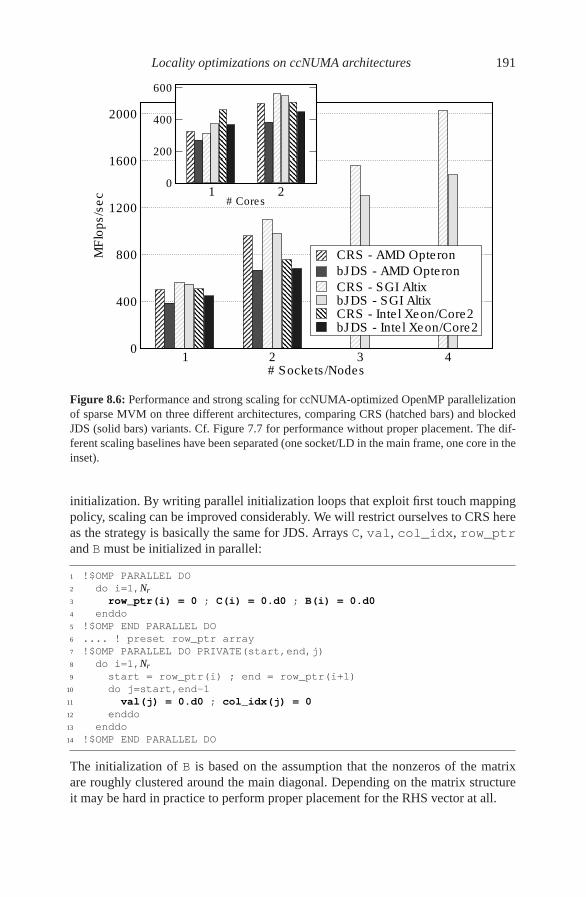
Locality optimizations on ccNUMA architectures 191
1 2 3 4# Sockets/Nodes
0
400
800
1200
1600
2000
MF
lops/s
ec
CRS - AMD Opteron
bJDS - AMD Opteron
CRS - SGI AltixbJDS - SGI AltixCRS - Intel Xeon/Core2bJDS - Intel Xeon/Core2
1 2# Cores
0
200
400
600
Figure 8.6: Performance and strong scaling for ccNUMA-optimized OpenMP parallelizationof sparse MVM on three different architectures, comparing CRS (hatched bars) and blockedJDS (solid bars) variants. Cf. Figure 7.7 for performance without proper placement. The dif-ferent scaling baselines have been separated (one socket/LD in the main frame, one core in theinset).
initialization. By writing parallel initialization loops that exploit first touch mappingpolicy, scaling can be improved considerably. We will restrict ourselves to CRS hereas the strategy is basically the same for JDS. Arrays C, val, col_idx, row_ptrand B must be initialized in parallel:
1 !$OMP PARALLEL DO
2 do i=1,Nr
3 row_ptr(i) = 0 ; C(i) = 0.d0 ; B(i) = 0.d0
4 enddo
5 !$OMP END PARALLEL DO
6 .... ! preset row_ptr array
7 !$OMP PARALLEL DO PRIVATE(start,end,j)
8 do i=1,Nr
9 start = row_ptr(i) ; end = row_ptr(i+1)
10 do j=start,end-1
11 val(j) = 0.d0 ; col_idx(j) = 0
12 enddo
13 enddo
14 !$OMP END PARALLEL DO
The initialization of B is based on the assumption that the nonzeros of the matrixare roughly clustered around the main diagonal. Depending on the matrix structureit may be hard in practice to perform proper placement for the RHS vector at all.

192 Introduction to High Performance Computing for Scientists and Engineers
Figure 8.6 shows performance data for the same architectures and sMVM codesas in Figure 7.7 but with appropriate ccNUMA placement. There is no change inscalability for the UMA platform, which was to be expected, but also on the cc-NUMA systems for up to two threads (see inset). The reason is of course that botharchitectures feature two-processor locality domains, which are of UMA type. Onfour threads and above, the locality optimizations yield dramatically improved per-formance. Especially for the CRS version scalability is nearly perfect when goingfrom 2n to 2(n + 1) threads (the scaling baseline in the main panel is the localitydomain or socket, respectively). The JDS variant of the code benefits from the opti-mizations as well, but falls behind CRS for larger thread numbers. This is becauseof the permutation map for JDS, which makes it hard to place larger portions of theRHS vector into the correct locality domains, and thus leads to increased NUMAtraffic.
8.3 Placement pitfalls
We have demonstrated that data placement is of premier importance on ccNUMAarchitectures, including commonly used two-socket cluster nodes. In principle, cc-NUMA offers superior scalability for memory-bound codes, but UMA systems aremuch easier to handle and require no code optimization for locality of access. Onecan expect, though, that ccNUMA designs will prevail in the commodity HPC mar-ket, where dual-socket configurations occupy a price vs. performance “sweet spot.”It must be emphasized, however, that the placement optimizations introduced in Sec-tion 8.1 may not always be applicable, e.g., when dynamic scheduling is unavoidable(see Section 8.3.1). Moreover, one may have arrived at the conclusion that placementproblems are restricted to shared-memory programming; this is entirely untrue andSection 8.3.2 will offer some more insight.
8.3.1 NUMA-unfriendly OpenMP scheduling
As explained in Sections 6.1.3 and 6.1.7, dynamic/guided loop scheduling andOpenMP task constructs could be preferable over static work distribution in poorlyload-balanced situations, if the additional overhead caused by frequently assigningtasks to threads is negligible. On the other hand, any sort of dynamic scheduling(including tasking) will necessarily lead to scalability problems if the thread team isspread across several locality domains. After all, the assignment of tasks to threads isunpredictable and even changes from run to run, which rules out an “optimal” pageplacement strategy.
Dropping parallel first touch altogether in such a situation is no solution as per-formance will then be limited by a single memory interface again. In order to get atleast a significant fraction of the maximum achievable bandwidth, it may be best todistribute the working set’s memory pages round-robin across the domains and hopefor a statistically even distribution of accesses. Again, the vector triad can serve as a

Locality optimizations on ccNUMA architectures 193
1 4 16 64 256 1024 4096 16384chunk size c [DP Words]
0
200
400
600
800
1000
Perf
orm
ance [M
Flo
ps/s
ec] static,c
round-robin placement
dynamic,cround-robin placement
4 kB page limit
static best placement
static LD0 placem.
Figure 8.7: Vector triadperformance vs. loopchunksize for static anddynamic scheduling witheight threads on a four-LD ccNUMA system(see Figure 8.3). Pageplacement was doneround-robin on purpose.Performance for bestparallel placement andLD0 placement withstatic scheduling isshown for reference.
convenient tool to fathom the impact of random page access. We modify the initial-ization loop by forcing static scheduling with a page-wide chunksize (assuming 4 kBpages):
1 ! initialization
2 !$OMP PARALLEL DO SCHEDULE(STATIC,512)
3 do i=1,N
4 A(i) = 0; B(i) = i; C(i) = mod(i,5); D(i) = mod(i,10)
5 enddo
6 !$OMP END PARALLEL DO
7 ...
8 do j=1,R
9 !$OMP PARALLEL DO SCHEDULE(RUNTIME)
10 do i=1,N
11 A(i) = B(i) + C(i) * D(i)
12 enddo
13 !$OMP END PARALLEL DO
14 call dummy(A,B,C,D)
15 enddo
By setting the OMP_SCHEDULE environment variable, different loop schedulingscan be tested. Figure 8.7 shows parallel triad performance versus chunksize c forstatic and dynamic scheduling, respectively, using eight threads on the four-socketccNUMA system from Figure8.3. At large c, where a single chunk spans severalmemory pages, performance converges asymptotically to a level governed by ran-dom access across all LDs, independent of the type of scheduling used. In this case,75% of all pages a thread needs reside in remote domains. Although this kind oferratic pattern bears at least a certain level of parallelism (compared with purely se-rial initialization as shown with the dashed line), there is almost a 50% performancepenalty versus the ideal case (solid line). The situation at c = 512 deserves someattention: With static scheduling, the access pattern of the triad loop matches theplacement policy from the initialization loop, enabling (mostly) local access in eachLD. The residual discrepancy to the best possible result can be attributed to the ar-
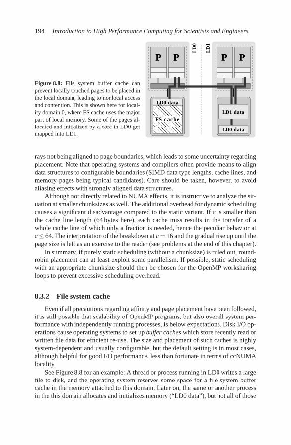
194 Introduction to High Performance Computing for Scientists and Engineers
Figure 8.8: File system buffer cache canprevent locally touched pages to be placed inthe local domain, leading to nonlocal accessand contention. This is shown here for local-ity domain 0, where FS cache uses the majorpart of local memory. Some of the pages al-located and initialized by a core in LD0 getmapped into LD1.
LD
0
LD
1
P P P P
�������������������������������������������������
�������������������������������������������������
LD1 data
LD0 data
LD0 data
FS cache
rays not being aligned to page boundaries, which leads to some uncertainty regardingplacement. Note that operating systems and compilers often provide means to aligndata structures to configurable boundaries (SIMD data type lengths, cache lines, andmemory pages being typical candidates). Care should be taken, however, to avoidaliasing effects with strongly aligned data structures.
Although not directly related to NUMA effects, it is instructive to analyze the sit-uation at smaller chunksizes as well. The additional overhead for dynamic schedulingcauses a significant disadvantage compared to the static variant. If c is smaller thanthe cache line length (64 bytes here), each cache miss results in the transfer of awhole cache line of which only a fraction is needed, hence the peculiar behavior atc≤ 64. The interpretation of the breakdown at c = 16 and the gradual rise up until thepage size is left as an exercise to the reader (see problems at the end of this chapter).
In summary, if purely static scheduling (without a chunksize) is ruled out, round-robin placement can at least exploit some parallelism. If possible, static schedulingwith an appropriate chunksize should then be chosen for the OpenMP worksharingloops to prevent excessive scheduling overhead.
8.3.2 File system cache
Even if all precautions regarding affinity and page placement have been followed,it is still possible that scalability of OpenMP programs, but also overall system per-formance with independently running processes, is below expectations. Disk I/O op-erations cause operating systems to set up buffer caches which store recently read orwritten file data for efficient re-use. The size and placement of such caches is highlysystem-dependent and usually configurable, but the default setting is in most cases,although helpful for good I/O performance, less than fortunate in terms of ccNUMAlocality.
See Figure 8.8 for an example: A thread or process running in LD0 writes a largefile to disk, and the operating system reserves some space for a file system buffercache in the memory attached to this domain. Later on, the same or another processin the this domain allocates and initializes memory (“LD0 data”), but not all of those

Locality optimizations on ccNUMA architectures 195
0 1000 2000 3000 4000FS buffer cache size S before running benchmark [MBytes]
0
100
200
300
400
500
Ag
g.
ve
cto
r tr
iad
pe
rfo
rma
nce
[M
Flo
ps/s
ec]
ccNUMA (Opteron dual-core 2 sockets)
UMA (Core2 dual-core 2 sockets)
Figure 8.9: Perfor-mance impact of a largefile system cache on accNUMA versus a UMAsystem (both with twosockets and four coresand 4 GB of RAM) whenrunning four concurrentvector triads. The buffercache was filled from asingle core. See text fordetails. (Benchmark databy Michael Meier.)
pages fit into LD0 together with the buffer cache. By default, many systems thenmap the excess pages to another locality domain so that, even though first touch wascorrectly employed from the programmer’s point of view, nonlocal access to LD0data and contention at LD1’s memory interface occurs.
A simple experiment can demonstrate this effect. We compare a UMA system(dual-core dual-socket Intel Xeon 5160 as in Figure 4.4) with a two-LD ccNUMAnode (dual-core dual-socket AMD Opteron as in Figure 4.5), both equipped with4 GB of main memory. On both systems we execute the following steps in a loop:
1. Write “dirty” data to disk and invalidate all the buffer cache. This step is highlysystem-dependent; usually there is a procedure that an administrator can exe-cute1 to do this, or a vendor-supplied library offers an option for it.
2. Write a file of size S to the local disk. The maximum file size equals the amountof memory. S should start at a very small size and be increased with everyiteration of this loop until it equals the system’s memory size.
3. Sync the cache so that there are no flush operations in the background (butthe cache is still filled). This can usually be done by the standard UNIX sync
command.
4. Run identical vector triad benchmarks on each core separately, using appropri-ate affinity mechanisms (see Appendix A). The aggregate size of all workingsets should equal half of the node’s memory. Report overall performance inMFlops/sec versus file size S (which equals the buffer cache size here).
The results are shown in Figure 8.9. On the UMA node, the buffer cache has certainlyno impact at all as there is no concept of locality. On the other hand, the ccNUMAsystem shows a strong performance breakdown with growing file size and hits rock
1On a current Linux OS, this can be done by executing the command echo 1 >
/proc/sys/vm/drop_caches. SGI Altix systems provide the bcfree command, which serves asimilar purpose.
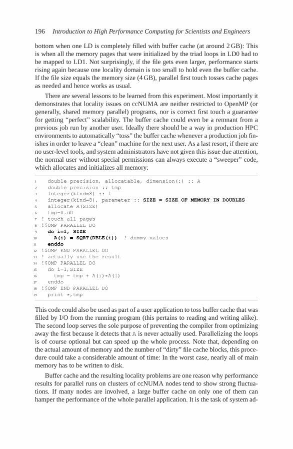
196 Introduction to High Performance Computing for Scientists and Engineers
bottom when one LD is completely filled with buffer cache (at around 2 GB): Thisis when all the memory pages that were initialized by the triad loops in LD0 had tobe mapped to LD1. Not surprisingly, if the file gets even larger, performance startsrising again because one locality domain is too small to hold even the buffer cache.If the file size equals the memory size (4 GB), parallel first touch tosses cache pagesas needed and hence works as usual.
There are several lessons to be learned from this experiment. Most importantly itdemonstrates that locality issues on ccNUMA are neither restricted to OpenMP (orgenerally, shared memory parallel) programs, nor is correct first touch a guaranteefor getting “perfect” scalability. The buffer cache could even be a remnant from aprevious job run by another user. Ideally there should be a way in production HPCenvironments to automatically “toss” the buffer cache whenever a production job fin-ishes in order to leave a “clean” machine for the next user. As a last resort, if there areno user-level tools, and system administrators have not given this issue due attention,the normal user without special permissions can always execute a “sweeper” code,which allocates and initializes all memory:
1 double precision, allocatable, dimension(:) :: A
2 double precision :: tmp
3 integer(kind=8) :: i
4 integer(kind=8), parameter :: SIZE = SIZE_OF_MEMORY_IN_DOUBLES
5 allocate A(SIZE)
6 tmp=0.d0
7 ! touch all pages
8 !$OMP PARALLEL DO
9 do i=1, SIZE
10 A(i) = SQRT(DBLE(i)) ! dummy values
11 enddo
12 !$OMP END PARALLEL DO
13 ! actually use the result
14 !$OMP PARALLEL DO
15 do i=1,SIZE
16 tmp = tmp + A(i)*A(1)
17 enddo
18 !$OMP END PARALLEL DO
19 print *,tmp
This code could also be used as part of a user application to toss buffer cache that wasfilled by I/O from the running program (this pertains to reading and writing alike).The second loop serves the sole purpose of preventing the compiler from optimizingaway the first because it detects that A is never actually used. Parallelizing the loopsis of course optional but can speed up the whole process. Note that, depending onthe actual amount of memory and the number of “dirty” file cache blocks, this proce-dure could take a considerable amount of time: In the worst case, nearly all of mainmemory has to be written to disk.
Buffer cache and the resulting locality problems are one reason why performanceresults for parallel runs on clusters of ccNUMA nodes tend to show strong fluctua-tions. If many nodes are involved, a large buffer cache on only one of them canhamper the performance of the whole parallel application. It is the task of system ad-
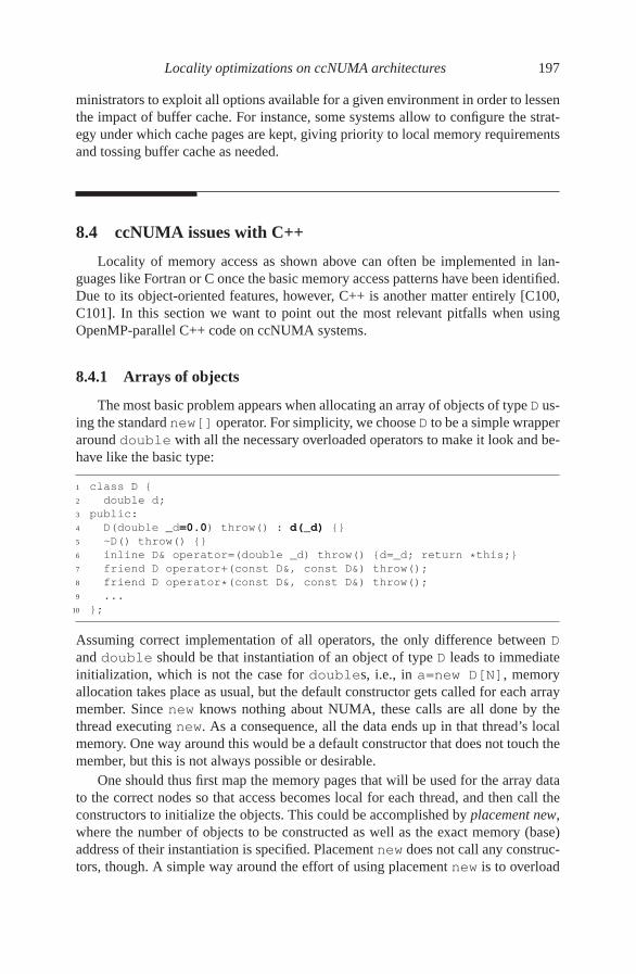
Locality optimizations on ccNUMA architectures 197
ministrators to exploit all options available for a given environment in order to lessenthe impact of buffer cache. For instance, some systems allow to configure the strat-egy under which cache pages are kept, giving priority to local memory requirementsand tossing buffer cache as needed.
8.4 ccNUMA issues with C++
Locality of memory access as shown above can often be implemented in lan-guages like Fortran or C once the basic memory access patterns have been identified.Due to its object-oriented features, however, C++ is another matter entirely [C100,C101]. In this section we want to point out the most relevant pitfalls when usingOpenMP-parallel C++ code on ccNUMA systems.
8.4.1 Arrays of objects
The most basic problem appears when allocating an array of objects of type D us-ing the standard new[] operator. For simplicity, we choose D to be a simple wrapperaround double with all the necessary overloaded operators to make it look and be-have like the basic type:
1 class D {
2 double d;
3 public:
4 D(double _d=0.0) throw() : d(_d) {}
5 ~D() throw() {}
6 inline D& operator=(double _d) throw() {d=_d; return *this;}
7 friend D operator+(const D&, const D&) throw();
8 friend D operator*(const D&, const D&) throw();
9 ...
10 };
Assuming correct implementation of all operators, the only difference between D
and double should be that instantiation of an object of type D leads to immediateinitialization, which is not the case for doubles, i.e., in a=new D[N], memoryallocation takes place as usual, but the default constructor gets called for each arraymember. Since new knows nothing about NUMA, these calls are all done by thethread executing new. As a consequence, all the data ends up in that thread’s localmemory. One way around this would be a default constructor that does not touch themember, but this is not always possible or desirable.
One should thus first map the memory pages that will be used for the array datato the correct nodes so that access becomes local for each thread, and then call theconstructors to initialize the objects. This could be accomplished by placement new,where the number of objects to be constructed as well as the exact memory (base)address of their instantiation is specified. Placement new does not call any construc-tors, though. A simple way around the effort of using placement new is to overload

198 Introduction to High Performance Computing for Scientists and Engineers
D::operator new[]. This operator has the sole responsibility to allocate “raw”memory. An overloaded version can, in addition to memory allocation, initialize thepages in parallel for good NUMA placement (we ignore the requirement to throwstd::bad_alloc on failure):
1 void* D::operator new[](size_t n) {
2 char *p = new char[n]; // allocate
3 size_t i,j;
4 #pragma omp parallel for private(j) schedule(runtime)
5 for(i=0; i<n; i += sizeof(D))
6 for(j=0; j<sizeof(D); ++j)
7 p[i+j] = 0;
8 return p;
9 }
10
11 void D::operator delete[](void* p) throw() {
12 delete [] static_cast<char*>p;
13 }
Construction of all objects in an array at their correct positions is then done automat-ically by the C++ runtime, using placement new. Note that the C++ runtime usuallyrequests a little more space than would be needed by the aggregated object sizes,which is used for storing administrative information alongside the actual data. Sincethe amount of data is small compared to NUMA-relevant array sizes, there is nonoticeable effect.
Overloading operator new[] works for simple cases like class D above.Dynamic members are problematic, however, because their NUMA locality cannotbe easily controlled:
1 class E {
2 size_t s;
3 std::vector<double> *v;
4 public:
5 E(size_t _s=100) : s(_s), v(new std::vector<double>(s)) {}
6 ~E() { delete [] v; }
7 ...
8 };
E’s constructor initializes E::s and E::v, and these would be the only data itemssubject to NUMA placement by an overloaded E::operator new[] upon con-struction of an array of E. The memory addressed by E::v is not handled by thismechanism; in fact, the std::vector<double> is preset upon construction in-side STL using copies of the object double(). This happens in the C++ runtimeafter E::operator new[] was executed. All the memory will be mapped into asingle locality domain.
Avoiding this situation is hardly possible with standard C++ and STL constructsif one insists on constructing arrays of objects with new[]. The best advice is to callobject constructors explicitly in a loop and to use a vector for holding pointers only:
1 std::vector<E*> v_E(n);
2

Locality optimizations on ccNUMA architectures 199
3 #pragma omp parallel for schedule(runtime)
4 for(size_t i=0; i<v_E.size(); ++i) {
5 v_E[i] = new E(100);
6 }
Since now the class constructor is called from different threads concurrently, it mustbe thread safe.
8.4.2 Standard Template Library
C-style array handling as shown in the previous section is certainly discouragedfor C++; the STL std::vector<> container is much safer and more convenient,but has its own problems with ccNUMA page placement. Even for simple data typeslike double, which have a trivial default constructor, placement is problematicsince, e.g., the allocated memory in a std::vector<>(int) object is filled withcopies of value_type() using std::uninitialized_fill(). The designof a dedicated NUMA-aware container class would probably allow for more ad-vanced optimizations, but STL defines a customizable abstraction layer called allo-
cators that can effectively encapsulate the low-level details of a container’s memorymanagement. By using this facility, correct NUMA placement can be enforced inmany cases for std::vector<> with minimal changes to an existing programcode.
STL containers have an optional template argument by which one can specify theallocator class to use [C102, C103]. By default, this is std::allocator<T>. Anallocator class provides, among others, the methods (class namespace omitted):
1 pointer allocate(size_type, const void *=0);
2 void deallocate(pointer, size_type);
Here size_type is size_t, and pointer is T*. The allocate() methodgets called by the container’s constructor to set up memory in much the same wayas operator new[] for an array of objects. However, since all relevant supple-mentary information is stored in additional member variables, the number of bytesto allocate matches the space required by the container’s contents only, at least oninitial construction (see below). The second parameter to allocate() can sup-ply additional information to the allocator, but its semantics are not standardized.deallocate() is responsible for freeing the allocated memory again.
The simplest NUMA-aware allocator would take care that allocate() notonly allocates memory but initializes it in parallel. For reference, Listing 8.1 showsthe code of a simple NUMA-friendly allocator, using standard malloc() for al-location. In line 19 the OpenMP API function omp_in_parallel() is used todetermine whether the allocator was called from an active parallel region. If it was,the initialization loop is skipped. To use the template, it must be specified as thesecond template argument whenever a std::vector<> object is constructed:
1 vector<double, NUMA_Allocator<double> > v(length);

200 Introduction to High Performance Computing for Scientists and Engineers
Listing 8.1: A NUMA allocator template. The implementation is somewhat simplified fromthe requirements in the C++ standard.
1 template <class T> class NUMA_Allocator {
2 public:
3 typedef T* pointer;
4 typedef const T* const_pointer;
5 typedef T& reference;
6 typedef const T& const_reference;
7 typedef size_t size_type;
8 typedef T value_type;
9
10 NUMA_Allocator() { }
11 NUMA_Allocator(const NUMA_Allocator& _r) { }
12 ~NUMA_Allocator() { }
13
14 // allocate raw memory including page placement
15 pointer allocate(size_type numObjects,
16 const void *localityHint=0) {
17 size_type len = numObjects * sizeof(value_type);
18 char *p = static_cast<char*>(std::malloc(len));
19 if(!omp_in_parallel()) {
20 #pragma omp parallel for schedule(runtime) private(ofs)
21 for(size_type i=0; i<len; i+=sizeof(value_type)) {
22 for(size_type j=0; j<sizeof(value_type); ++j) {
23 p[i+j]=0;
24 }
25 }
26 return static_cast<pointer>(m);
27 }
28
29 // free raw memory
30 void deallocate(pointer ptrToMemory, size_type numObjects) {
31 std::free(ptrToMemory);
32 }
33
34 // construct object at given address
35 void construct(pointer p, const value_type& x) {
36 new(p) value_type(x);
37 }
38
39 // destroy object at given address
40 void destroy(pointer p) {
41 p-> value_type();
42 }
43
44 private:
45 void operator=(const NUMA_Allocator&) {}
46 };

Locality optimizations on ccNUMA architectures 201
What follows after memory allocation is pretty similar to the array-of-objectscase, and has the same restrictions: The allocator’s construct() method is calledFor each of the objects, and uses placement new to construct each object at thecorrect address (line 36). Upon destruction, each object’s destructor is called ex-plicitly (one of the rare cases where this is necessary) via the destroy() methodin line 41. Note that container construction and destruction are not the only placeswhere construct() and destroy() are invoked, and that there are many thingswhich could destroy NUMA locality immediately. For instance, due to the conceptof container size versus capacity, calling std::vector<>::push_back() justonce on a “filled” container reallocates all memory plus a significant amount more,and copies the original objects to their new locations. The NUMA allocator will per-form first-touch placement, but it will do so using the container’s new capacity, not itssize. As a consequence, placement will almost certainly be suboptimal. One shouldkeep in mind that not all the functionality of std::vector<> is suitable to usein a ccNUMA environment. We are not even talking about the other STL containers(deque, list, map, set, etc.).
Incidentally, standard-compliant allocator objects of the same type must alwayscompare as equal [C102]:
1 template <class T>
2 inline bool operator==(const NUMA_Allocator<T>&,
3 const NUMA_Allocator<T>&) { return true; }
4 template <class T>
5 inline bool operator!=(const NUMA_Allocator<T>&,
6 const NUMA_Allocator<T>&) { return false; }
This has the important consequence that an allocator object is necessarily state-less, ruling out some optimizations one may think of. A template specialization forT=void must also be provided (not shown here). These and other peculiarities arediscussed in the literature. More sophisticated strategies than using plain malloc()do of course exist.
In summary we must add that the methods shown here are useful for outfittingexisting C++ programs with some ccNUMA awareness without too much hassle.Certainly a newly designed code should be parallelized with ccNUMA in mind fromthe start.
Problems
For solutions see page 303 ff.
8.1 Dynamic scheduling and ccNUMA. When a memory-bound, OpenMP-parallelcode runs on all sockets of a ccNUMA system, one should use static schedulingand initialize the data in parallel to make sure that memory accesses are mostlylocal. We want to analyze what happens if static scheduling is not a option, e.g.,for load balancing reasons.

202 Introduction to High Performance Computing for Scientists and Engineers
For a system with two locality domains, calculate the expected performanceimpact of dynamic scheduling on a memory-bound parallel loop. Assume forsimplicity that there is exactly one thread (core) running per LD. This thread isable to saturate the local or any remote memory bus with some performance p.The inter-LD network should be infinitely fast, i.e., there is no penalty for non-local transfers and no contention effects on the inter-LD link. Further assumethat all pages are homogeneously distributed throughout the system and thatdynamic scheduling is purely statistical (i.e., each thread accesses all LDs ina random manner, with equal probability). Finally, assume that the chunksizeis large enough so that there are no bad effects from hardware prefetching orpartial cache line use.
The code’s performance with static scheduling and perfect load balance wouldbe 2p. What is the expected performance under dynamic scheduling (also withperfect load balance)?
8.2 Unfortunate chunksizes. What could be possible reasons for the performancebreakdown at chunksizes between 16 and 256 for the parallel vector triad on afour-LD ccNUMA machine (Figure 8.7)? Hint: Memory pages play a decisiverole here.
8.3 Speeding up “small” jobs. If a ccNUMA system is sparsely utilized, e.g., ifthere are less threads than locality domains, and they all execute (memory-bound) code, is the first touch policy still the best strategy for page placement?
8.4 Triangular matrix-vector multiplication. Parallelize a triangular matrix-vectormultiplication using OpenMP:
1 do r=1,N
2 do c=1,r
3 y(r) = y(r) + a(c,r) * x(c)
4 enddo
5 enddo
What is the central parallel performance issue here? How can it be solved ingeneral, and what special precautions are necessary on ccNUMA systems?You may ignore the standard scalar optimizations (unrolling, blocking).
8.5 NUMA placement by overloading. In Section 8.4.1 we enforced NUMA place-ment for arrays of objects of type D by overloading D::operator new[].A similar thing was done in the NUMA-aware allocator class (Listing 8.1).Why did we use a loop nest for memory initialization instead of a single loopover i?

Chapter 9
Distributed-memory parallel programmingwith MPI
Ever since parallel computers hit the HPC market, there was an intense discussionabout what should be an appropriate programming model for them. The use of ex-plicit message passing (MP), i.e., communication between processes, is surely themost tedious and complicated but also the most flexible parallelization method. Paral-lel computer vendors recognized the wish for efficient message-passing facilities, andprovided proprietary, i.e., nonportable libraries up until the early 1990s. At that pointin time it was clear that a joint standardization effort was required to enable scientificusers to write parallel programs that were easily portable between platforms. The re-sult of this effort was MPI, the Message Passing Interface. Today, the MPI standardis supported by several free and commercial implementations [W125, W126, W127],and has been extended several times. It contains not only communication routines,but also facilities for efficient parallel I/O (if supported by the underlying hardware).An MPI library is regarded as a necessary ingredient in any HPC system installation,and numerous types of interconnect are supported.
The current MPI standard in version 2.2 (to which we always refer in this book)defines over 500 functions, and it is beyond the scope of this book to even try to coverthem all. In this chapter we will concentrate on the important concepts of messagepassing and MPI in particular, and provide some knowledge that will enable thereader to consult more advanced textbooks [P13, P14] or the standard documentitself [W128, P15].
9.1 Message passing
Message passing is required if a parallel computer is of the distributed-memorytype, i.e., if there is no way for one processor to directly access the address spaceof another. However, it can also be regarded as a programming model and usedon shared-memory or hybrid systems as well (see Chapter 4 for a categorization).MPI, the nowadays dominating message-passing standard, conforms to the follow-ing rules:
• The same program runs on all processes (Single Program Multiple Data, orSPMD). This is no restriction compared to the more general MPMD (MultipleProgram Multiple Data) model as all processes taking part in a parallel calcu-
203

204 Introduction to High Performance Computing for Scientists and Engineers
lation can be distinguished by a unique identifier called rank (see below). Mostmodern MPI implementations allow starting different binaries in different pro-cesses, however. An MPMD-style message passing library is PVM, the ParallelVirtual Machine [P16]. Since it has waned in importance in recent years, it willnot be covered here.
• The program is written in a sequential language like Fortran, C or C++. Dataexchange, i.e., sending and receiving of messages, is done via calls to an ap-propriate library.
• All variables in a process are local to this process. There is no concept ofshared memory.
One should add that message passing is not the only possible programming paradigmfor distributed-memory machines. Specialized languages like High Performance For-tran (HPF), Co-Array Fortran (CAF) [P17], Unified Parallel C (UPC) [P18], etc.,have been created with support for distributed-memory parallelization built in, butthey have not developed a broad user community and it is as yet unclear whetherthose approaches can match the efficiency of MPI.
In a message passing program, messages carry data between processes. Thoseprocesses could be running on separate compute nodes, or different cores inside anode, or even on the same processor core, time-sharing its resources. A messagecan be as simple as a single item (like a DP word) or even a complicated structure,perhaps scattered all over the address space. For a message to be transmitted in anorderly manner, some parameters have to be fixed in advance:
• Which process is sending the message?
• Where is the data on the sending process?
• What kind of data is being sent?
• How much data is there?
• Which process is going to receive the message?
• Where should the data be left on the receiving process?
• What amount of data is the receiving process prepared to accept?
All MPI calls that actually transfer data have to specify those parameters in someway. Note that above parameters strictly relate to point-to-point communication,where there is always exactly one sender and one receiver. As we will see, MPI sup-ports much more than just sending a single message between two processes; there isa similar set of parameters for those more complex cases as well.
MPI is a very broad standard with a huge number of library routines. Fortunately,most applications merely require less than a dozen of those.

Distributed-memory parallel programming with MPI 205
Listing 9.1: A very simple, fully functional “Hello World” MPI program in Fortran 90.
1 program mpitest
2
3 use MPI
4
5 integer :: rank, size, ierror
6
7 call MPI_Init(ierror)
8 call MPI_Comm_size(MPI_COMM_WORLD, size, ierror)
9 call MPI_Comm_rank(MPI_COMM_WORLD, rank, ierror)
10
11 write(*,*) ’Hello World, I am ’,rank,’ of ’,size
12
13 call MPI_Finalize(ierror)
14 end
9.2 A short introduction to MPI
9.2.1 A simple example
MPI is always available as a library. In order to compile and link an MPI program,compilers and linkers need options that specify where include files (i.e., C headersand Fortran modules) and libraries can be found. As there is considerable variationin those locations among installations, most MPI implementations provide compilerwrapper scripts (often called mpicc, mpif77, etc.), which supply the required op-tions automatically but otherwise behave like “normal” compilers. Note that the waythat MPI programs should be compiled and started is not fixed by the standard, soplease consult the system documentation by all means.
Listing 9.1 shows a simple “Hello World”-type MPI program in Fortran 90. (SeeListing 9.2 for a C version. We will mostly stick to the Fortran MPI bindings, andonly describe the differences to C where appropriate. Although there are C++ bind-ings defined by the standard, they are of limited usefulness and will thus not becovered here. In fact, they are deprecated as of MPI 2.2.) In line 3, the MPI mod-ule is loaded, which provides required globals and definitions (the preprocessor isused to read in the mpi.h header in C; there is an equivalent header file for Fortran77 called mpif.h). All Fortran MPI calls take an INTENT(OUT) argument, herecalled ierror, which transports information about the success of the MPI operationto the user code, a value of MPI_SUCCESS meaning that there were no errors. In C,the return code is used for that, and the ierror argument does not exist. Since fail-ure resiliency is not built into the MPI standard today and checkpoint/restart featuresare usually implemented by the user code anyway, the error code is rarely used at allin practice.
The first statement, apart from variable declarations, in any MPI code should be
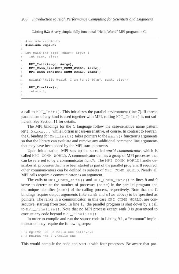
206 Introduction to High Performance Computing for Scientists and Engineers
Listing 9.2: A very simple, fully functional “Hello World” MPI program in C.
1 #include <stdio.h>
2 #include <mpi.h>
3
4 int main(int argc, char** argv) {
5 int rank, size;
6
7 MPI_Init(&argc, &argv);
8 MPI_Comm_size(MPI_COMM_WORLD, &size);
9 MPI_Comm_rank(MPI_COMM_WORLD, &rank);
10
11 printf("Hello World, I am %d of %d\n", rank, size);
12
13 MPI_Finalize();
14 return 0;
15 }
a call to MPI_Init(). This initializes the parallel environment (line 7). If threadparallelism of any kind is used together with MPI, calling MPI_Init() is not suf-ficient. See Section 11 for details.
The MPI bindings for the C language follow the case-sensitive name patternMPI_Xxxxx..., while Fortran is case-insensitive, of course. In contrast to Fortran,the C binding for MPI_Init() takes pointers to the main() function’s argumentsso that the library can evaluate and remove any additional command line argumentsthat may have been added by the MPI startup process.
Upon initialization, MPI sets up the so-called world communicator, which iscalled MPI_COMM_WORLD. A communicator defines a group of MPI processes thatcan be referred to by a communicator handle. The MPI_COMM_WORLD handle de-scribes all processes that have been started as part of the parallel program. If required,other communicators can be defined as subsets of MPI_COMM_WORLD. Nearly allMPI calls require a communicator as an argument.
The calls to MPI_Comm_size() and MPI_Comm_rank() in lines 8 and 9serve to determine the number of processes (size) in the parallel program andthe unique identifier (rank) of the calling process, respectively. Note that the Cbindings require output arguments (like rank and size above) to be specified aspointers. The ranks in a communicator, in this case MPI_COMM_WORLD, are con-secutive, starting from zero. In line 13, the parallel program is shut down by a callto MPI_Finalize(). Note that no MPI process except rank 0 is guaranteed toexecute any code beyond MPI_Finalize().
In order to compile and run the source code in Listing 9.1, a “common” imple-mentation may require the following steps:
1 $ mpif90 -O3 -o hello.exe hello.F90
2 $ mpirun -np 4 ./hello.exe
This would compile the code and start it with four processes. Be aware that pro-
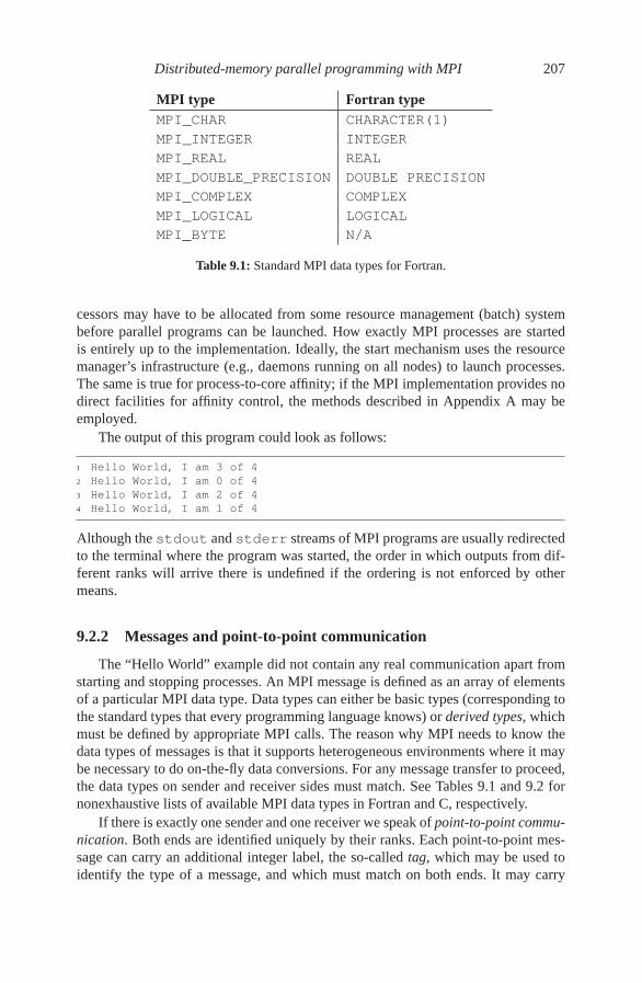
Distributed-memory parallel programming with MPI 207
MPI type Fortran type
MPI_CHAR CHARACTER(1)
MPI_INTEGER INTEGER
MPI_REAL REAL
MPI_DOUBLE_PRECISION DOUBLE PRECISION
MPI_COMPLEX COMPLEX
MPI_LOGICAL LOGICAL
MPI_BYTE N/A
Table 9.1: Standard MPI data types for Fortran.
cessors may have to be allocated from some resource management (batch) systembefore parallel programs can be launched. How exactly MPI processes are startedis entirely up to the implementation. Ideally, the start mechanism uses the resourcemanager’s infrastructure (e.g., daemons running on all nodes) to launch processes.The same is true for process-to-core affinity; if the MPI implementation provides nodirect facilities for affinity control, the methods described in Appendix A may beemployed.
The output of this program could look as follows:
1 Hello World, I am 3 of 4
2 Hello World, I am 0 of 4
3 Hello World, I am 2 of 4
4 Hello World, I am 1 of 4
Although the stdout and stderr streams of MPI programs are usually redirectedto the terminal where the program was started, the order in which outputs from dif-ferent ranks will arrive there is undefined if the ordering is not enforced by othermeans.
9.2.2 Messages and point-to-point communication
The “Hello World” example did not contain any real communication apart fromstarting and stopping processes. An MPI message is defined as an array of elementsof a particular MPI data type. Data types can either be basic types (corresponding tothe standard types that every programming language knows) or derived types, whichmust be defined by appropriate MPI calls. The reason why MPI needs to know thedata types of messages is that it supports heterogeneous environments where it maybe necessary to do on-the-fly data conversions. For any message transfer to proceed,the data types on sender and receiver sides must match. See Tables 9.1 and 9.2 fornonexhaustive lists of available MPI data types in Fortran and C, respectively.
If there is exactly one sender and one receiver we speak of point-to-point commu-
nication. Both ends are identified uniquely by their ranks. Each point-to-point mes-sage can carry an additional integer label, the so-called tag, which may be used toidentify the type of a message, and which must match on both ends. It may carry

208 Introduction to High Performance Computing for Scientists and Engineers
MPI type C type
MPI_CHAR signed char
MPI_INT signed int
MPI_LONG signed long
MPI_FLOAT float
MPI_DOUBLE double
MPI_BYTE N/A
Table 9.2: A selection of the standard MPI data types for C. Unsigned variants exist whereapplicable.
any accompanying information, or just be set to some constant value if it is notneeded. The basic MPI function to send a message from one process to another isMPI_Send():
1 <type> buf(*)
2 integer :: count, datatype, dest, tag, comm, ierror
3 call MPI_Send(buf, ! message buffer
4 count, ! # of items
5 datatype, ! MPI data type
6 dest, ! destination rank
7 tag, ! message tag (additional label)
8 comm, ! communicator
9 ierror) ! return value
The data type of the message buffer may vary; the MPI interfaces and prototypesdeclared in modules and headers accommodate this.1 A message may be receivedwith the MPI_Recv() function:
1 <type> buf(*)
2 integer :: count, datatype, source, tag, comm,
3 integer :: status(MPI_STATUS_SIZE), ierror
4 call MPI_Recv(buf, ! message buffer
5 count, ! maximum # of items
6 datatype, ! MPI data type
7 source, ! source rank
8 tag, ! message tag (additional label)
9 comm, ! communicator
10 status, ! status object (MPI_Status* in C)
11 ierror) ! return value
Compared with MPI_Send(), this function has an additional output argument,the status object. After MPI_Recv() has returned, the status object can beused to determine parameters that have not been fixed by the call’s arguments. Pri-marily, this pertains to the length of the message, because the count parameter is
1While this is no problem in C/C++, where the void* pointer type conveniently hides any variationin the argument type, the Fortran MPI bindings are explicitly inconsistent with the language standard.However, this can be tolerated in most cases. See the standard document [P15] for details.

Distributed-memory parallel programming with MPI 209
only a maximum value at the receiver side; the message may be shorter than countelements. The MPI_Get_count() function can retrieve the real number:
1 integer :: status(MPI_STATUS_SIZE), datatype, count, ierror
2 call MPI_Get_count(status, ! status object from MPI_Recv()
3 datatype, ! MPI data type received
4 count, ! count (output argument)
5 ierror) ! return value
However, the status object also serves another purpose.The source and tag ar-guments of MPI_Recv() may be equipped with the special constants (“wildcards”)MPI_ANY_SOURCE and MPI_ANY_TAG, respectively. The former specifies thatthe message may be sent by anyone, while the latter determines that the message tagshould not matter. After MPI_Recv() has returned, status(MPI_SOURCE) andstatus(MPI_TAG) contain the sender’s rank and the message tag, respectively.(In C, the status object is of type struct MPI_Status, and access to sourceand tag information works via the “.” operator.)
Note that MPI_Send() and MPI_Recv() have blocking semantics, meaningthat the buffer can be used safely after the function returns (i.e., it can be modifiedafter MPI_Send() without altering any message in flight, and one can be sure thatthe message has been completely received after MPI_Recv()). This is not to beconfused with synchronous behavior; see below for details.
Listing 9.3 shows an MPI program fragment for computing an integral over somefunction f(x) in parallel. In contrast to the OpenMP version in Listing 6.2, the dis-tribution of work among processes must be handled manually in MPI. Each MPIprocess gets assigned a subinterval of the integration domain according to its rank(lines 9 and 10), and some other function integrate(), which may look simi-lar to Listing 6.2, can then perform the actual integration (line 13). After that eachprocess holds its own partial result, which should be added to get the final inte-gral. This is done at rank 0, who executes a loop over all ranks from 1 to size−1(lines 18–29), receiving the local integral from each rank in turn via MPI_Recv()(line 19) and accumulating the result in res (line 28). Each rank apart from 0has to call MPI_Send() to transmit the data. Hence, there are size− 1 sendand size− 1 matching receive operations. The data types on both sides are spec-ified to be MPI_DOUBLE_PRECISION, which corresponds to the usual doubleprecision type in Fortran (cf. Table 9.1). The message tag is not used here, so weset it to zero.
This simple program could be improved in several ways:
• MPI does not preserve the temporal order of messages unless they are trans-mitted between the same sender/receiver pair (and with the same tag). Hence,to allow the reception of partial results at rank 0 without delay due to differentexecution times of the integrate() function, it may be better to use theMPI_ANY_SOURCE wildcard instead of a definite source rank in line 23.
• Rank 0 does not call MPI_Recv() before returning from its own executionof integrate(). If other processes finish their tasks earlier, communica-tion cannot proceed, and it cannot be overlapped with computation. The MPI

210 Introduction to High Performance Computing for Scientists and Engineers
Listing 9.3: Program fragment for parallel integration in MPI.
1 integer, dimension(MPI_STATUS_SIZE) :: status
2 call MPI_Comm_size(MPI_COMM_WORLD, size, ierror)
3 call MPI_Comm_rank(MPI_COMM_WORLD, rank, ierror)
4
5 ! integration limits
6 a=0.d0 ; b=2.d0 ; res=0.d0
7
8 ! limits for "me"
9 mya=a+rank*(b-a)/size
10 myb=mya+(b-a)/size
11
12 ! integrate f(x) over my own chunk - actual work
13 psum = integrate(mya,myb)
14
15 ! rank 0 collects partial results
16 if(rank.eq.0) then
17 res=psum
18 do i=1,size-1
19 call MPI_Recv(tmp, & ! receive buffer
20 1, & ! array length
21 ! data type
22 MPI_DOUBLE_PRECISION,&
23 i, & ! rank of source
24 0, & ! tag (unused here)
25 MPI_COMM_WORLD,& ! communicator
26 status,& ! status array (msg info)
27 ierror)
28 res=res+tmp
29 enddo
30 write(*,*) ’Result: ’,res
31 ! ranks != 0 send their results to rank 0
32 else
33 call MPI_Send(psum, & ! send buffer
34 1, & ! message length
35 MPI_DOUBLE_PRECISION,&
36 0, & ! rank of destination
37 0, & ! tag (unused here)
38 MPI_COMM_WORLD,ierror)
39 endif

Distributed-memory parallel programming with MPI 211
SendRecv
SendRecv
SendRecv
SendRecv
SendRecv
SendRecv
0 5
4
32
1
Figure 9.1: A ring shift communication pattern. If sends and receives are performed in theorder shown, a deadlock can occur because MPI_Send() may be synchronous.
standard provides nonblocking point-to-point communication facilities that al-low multiple outstanding receives (and sends), and even let implementationssupport asynchronous messages. See Section 9.2.4 for more information.
• Since the final result is needed at rank 0, this process is necessarily a commu-nication bottleneck if the number of messages gets large. In Section 10.4.4 wewill demonstrate optimizations that can significantly reduce communicationoverhead in those situations. Fortunately, nobody is required to write explicitcode for this. In fact, the global sum is an example for a reduction operation
and is well supported within MPI (see Section 9.2.3). Vendor implementationsare assumed to provide optimized versions of such global operations.
While MPI_Send() is easy to use, one should be aware that the MPI standardallows for a considerable amount of freedom in its actual implementation. Internallyit may work completely synchronously, meaning that the call can not return to theuser code before a message transfer has at least started after a handshake with thereceiver. However, it may also copy the message to an intermediate buffer and returnright away, leaving the handshake and data transmission to another mechanism, likea background thread. It may even change its behavior depending on any explicitor hidden parameters. Apart from a possible performance impact, deadlocks mayoccur if the possible synchronousness of MPI_Send() is not taken into account. Atypical communication pattern where this may become crucial is a “ring shift” (seeFigure 9.1). All processes form a closed ring topology, and each first sends a messageto its “left-hand” and then receives a message from its “right-hand” neighbor:
1 integer :: size, rank, left, right, ierror
2 integer, dimension(N) :: buf
3 call MPI_Comm_size(MPI_COMM_WORLD, size, ierror)
4 call MPI_Comm_rank(MPI_COMM_WORLD, rank, ierror)
5 left = rank+1 ! left and right neighbors
6 right = rank-1
7 if(right<0) right=size-1 ! close the ring
8 if(left>=size) left=0
9 call MPI_Send(buf, N, MPI_INTEGER, left, 0, &
10 MPI_COMM_WORLD,ierror)
11 call MPI_Recv(buf,N,MPI_INTEGER,right,0, &
12 MPI_COMM_WORLD,status,ierror)

212 Introduction to High Performance Computing for Scientists and Engineers
RecvSend
SendRecv
SendRecv
RecvSend
SendRecv
RecvSend
0 5
4
32
1
Figure 9.2: A possible solution for the deadlock problem with the ring shift: By changingthe order of MPI_Send() and MPI_Recv() on all odd-numbered ranks, pairs of processescan communicate without deadlocks because there is now a matching receive for every sendoperation (dashed boxes).
If MPI_Send() is synchronous, all processes call it first and then wait forever un-til a matching receive gets posted. However, it may well be that the ring shift runswithout problems if the messages are sufficiently short. In fact, most MPI implemen-tations provide a (small) internal buffer for short messages and switch to synchronousmode when the buffer is full or too small (the situation is actually a little more com-plex in reality; see Sections 10.2 and 10.3 for details). This may lead to sporadicdeadlocks, which are hard to spot. If there is some suspicion that a sporadic deadlockis triggered by MPI_Send() switching to synchronous mode, one can substitute alloccurrences of MPI_Send() by MPI_Ssend(), which has the same interface butis synchronous by definition.
A simple solution to this deadlock problem is to interchange the MPI_Send()and MPI_Recv() calls on, e.g., all odd-numbered processes, so that there is amatching receive for every send executed (see Figure 9.2). Lines 9–12 in the codeabove should thus be replaced by:
1 if(MOD(rank,2)/=0) then
2 call MPI_Recv(buf,N,MPI_INTEGER,right,0, & ! odd rank
3 MPI_COMM_WORLD,status,ierror)
4 call MPI_Send(buf, N, MPI_INTEGER, left, 0, &
5 MPI_COMM_WORLD,ierror)
6 else
7 call MPI_Send(buf, N, MPI_INTEGER, left, 0, & ! even rank
8 MPI_COMM_WORLD,ierror)
9 call MPI_Recv(buf,N,MPI_INTEGER,right,0, &
10 MPI_COMM_WORLD,status,ierror)
11 endif
After the messages sent by the even ranks have been transmitted, the remainingsend/receive pairs can be matched as well. This solution does not exploit the fullbandwidth of a nonblocking network, however, because only half the possible com-munication links can be active at any time (at least if MPI_Send() is really syn-chronous). A better alternative is the use of nonblocking communication. See Sec-tion 9.2.4 for more information, and Problem 9.1 for some more aspects of the ringshift pattern.
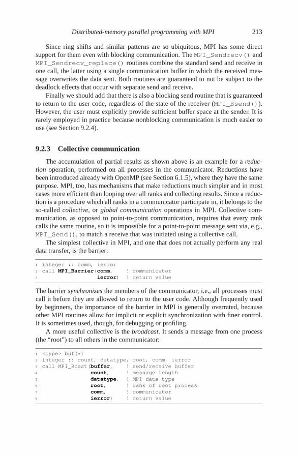
Distributed-memory parallel programming with MPI 213
Since ring shifts and similar patterns are so ubiquitous, MPI has some directsupport for them even with blocking communication. The MPI_Sendrecv() andMPI_Sendrecv_replace() routines combine the standard send and receive inone call, the latter using a single communication buffer in which the received mes-sage overwrites the data sent. Both routines are guaranteed to not be subject to thedeadlock effects that occur with separate send and receive.
Finally we should add that there is also a blocking send routine that is guaranteedto return to the user code, regardless of the state of the receiver (MPI_Bsend()).However, the user must explicitly provide sufficient buffer space at the sender. It israrely employed in practice because nonblocking communication is much easier touse (see Section 9.2.4).
9.2.3 Collective communication
The accumulation of partial results as shown above is an example for a reduc-
tion operation, performed on all processes in the communicator. Reductions havebeen introduced already with OpenMP (see Section 6.1.5), where they have the samepurpose. MPI, too, has mechanisms that make reductions much simpler and in mostcases more efficient than looping over all ranks and collecting results. Since a reduc-tion is a procedure which all ranks in a communicator participate in, it belongs to theso-called collective, or global communication operations in MPI. Collective com-munication, as opposed to point-to-point communication, requires that every rankcalls the same routine, so it is impossible for a point-to-point message sent via, e.g.,MPI_Send(), to match a receive that was initiated using a collective call.
The simplest collective in MPI, and one that does not actually perform any realdata transfer, is the barrier:
1 integer :: comm, ierror
2 call MPI_Barrier(comm, ! communicator
3 ierror) ! return value
The barrier synchronizes the members of the communicator, i.e., all processes mustcall it before they are allowed to return to the user code. Although frequently usedby beginners, the importance of the barrier in MPI is generally overrated, becauseother MPI routines allow for implicit or explicit synchronization with finer control.It is sometimes used, though, for debugging or profiling.
A more useful collective is the broadcast. It sends a message from one process(the “root”) to all others in the communicator:
1 <type> buf(*)
2 integer :: count, datatype, root, comm, ierror
3 call MPI_Bcast(buffer, ! send/receive buffer
4 count, ! message length
5 datatype, ! MPI data type
6 root, ! rank of root process
7 comm, ! communicator
8 ierror) ! return value
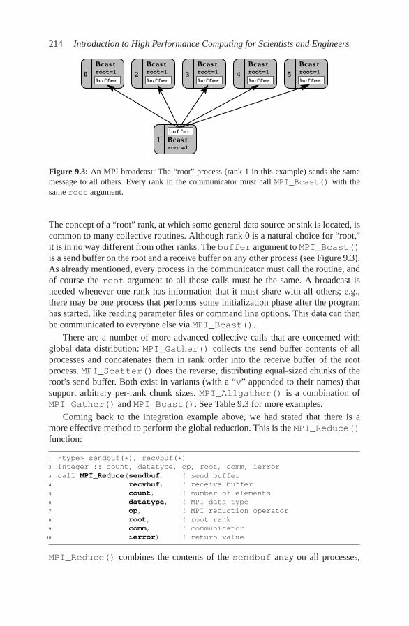
214 Introduction to High Performance Computing for Scientists and Engineers
1root=1
Bcast
root=10
Bcastroot=13
Bcastroot=14
Bcastroot=15
Bcastroot=12
Bcast
buffer
buffer buffer buffer bufferbuffer
Figure 9.3: An MPI broadcast: The “root” process (rank 1 in this example) sends the samemessage to all others. Every rank in the communicator must call MPI_Bcast() with thesame root argument.
The concept of a “root” rank, at which some general data source or sink is located, iscommon to many collective routines. Although rank 0 is a natural choice for “root,”it is in no way different from other ranks. The buffer argument to MPI_Bcast()is a send buffer on the root and a receive buffer on any other process (see Figure 9.3).As already mentioned, every process in the communicator must call the routine, andof course the root argument to all those calls must be the same. A broadcast isneeded whenever one rank has information that it must share with all others; e.g.,there may be one process that performs some initialization phase after the programhas started, like reading parameter files or command line options. This data can thenbe communicated to everyone else via MPI_Bcast().
There are a number of more advanced collective calls that are concerned withglobal data distribution: MPI_Gather() collects the send buffer contents of allprocesses and concatenates them in rank order into the receive buffer of the rootprocess. MPI_Scatter() does the reverse, distributing equal-sized chunks of theroot’s send buffer. Both exist in variants (with a “v” appended to their names) thatsupport arbitrary per-rank chunk sizes. MPI_Allgather() is a combination ofMPI_Gather() and MPI_Bcast(). See Table 9.3 for more examples.
Coming back to the integration example above, we had stated that there is amore effective method to perform the global reduction. This is the MPI_Reduce()function:
1 <type> sendbuf(*), recvbuf(*)
2 integer :: count, datatype, op, root, comm, ierror
3 call MPI_Reduce(sendbuf, ! send buffer
4 recvbuf, ! receive buffer
5 count, ! number of elements
6 datatype, ! MPI data type
7 op, ! MPI reduction operator
8 root, ! root rank
9 comm, ! communicator
10 ierror) ! return value
MPI_Reduce() combines the contents of the sendbuf array on all processes,

Distributed-memory parallel programming with MPI 215
root=1count=4op=MPI_SUM
Reduce
root=1count=4op=MPI_SUM
Reduce
root=1count=4op=MPI_SUM
Reduce
root=1count=4op=MPI_SUM
Reducesendbuf
recvbuf
0
2
3
sendbuf
sendbuf
sendbuf
1+ + + +
Figure 9.4: A reductionon an array of lengthcount (a sum in thisexample) is performedby MPI_Reduce().Every process mustprovide a send buffer.The receive buffer ar-gument is only used onthe root process. Thelocal copy on root canbe prevented by speci-fying MPI_IN_PLACE
instead of a send bufferaddress.
element-wise, using an operator encoded by the op argument, and stores the result inrecvbuf on root (see Figure 9.4). There are twelve predefined operators, the mostimportant being MPI_MAX, MPI_MIN, MPI_SUM and MPI_PROD, which imple-ment the global maximum, minimum, sum, and product, respectively. User-definedoperators are also supported.
Now it is clear that the whole if . . .else . . .endif construct between lines16 and 39 in Listing 9.3 (apart from printing the result in line 30) could have beenwritten as follows:
1 call MPI_Reduce(psum, & ! send buffer (partial result)
2 res, & ! recv buffer (final result @ root)
3 1, & ! array length
4 MPI_DOUBLE_PRECISION, &
5 MPI_SUM, & ! type of operation
6 0, & ! root (accumulate result there)
7 MPI_COMM_WORLD,ierror)
Although a receive buffer (the res variable here) must be specified on all ranks,it is only relevant (and used) on root. Note that MPI_Reduce() in its plain formrequires separate send and receive buffers on the root process. If allowed by theprogram semantics, the local accumulation on root can be simplified by setting thesendbuf argument to the special constant MPI_IN_PLACE. recvbuf is thenused as the send buffer and gets overwritten with the global result. This can be goodfor performance if count is large and the additional copy operation leads to signifi-cant overhead. The behavior of the call on all nonroot processes is unchanged.
There are a few more global operations related to MPI_Reduce()worth noting.

216 Introduction to High Performance Computing for Scientists and Engineers
���������������������������������������������
���������������������������������������������
use bufWait()Isend(buf)Main thread
Auxiliary thread
buf)
post send operation, handshake, data transfer
do other work (not using
SY
NC
time
Figure 9.5: Abstract timeline view of a nonblocking send (MPI_Isend()). Whether there isactually an auxiliary thread is not specified by the standard; the whole data transfer may takeplace during MPI_Wait() or any other MPI function.
For example, MPI_Allreduce() is a fusion of a reduction with a broadcast, andMPI_Reduce_scatter() combines MPI_Reduce()with MPI_Scatter().
Note that collectives are not required to, but still may synchronize all processes(the barrier is synchronizing by definition, of course). They are thus prone to similardeadlock hazards as blocking point-to-point communication (see above). This means,e.g., that collectives must be executed by all processes in the same order. See the MPIstandard document [P15] for examples.
In general it is a good idea to prefer collectives over point-to-point constructsor combinations of simpler collectives that “emulate” the same semantics (see alsoFigures 10.15 and 10.16 and the corresponding discussion in Section 10.4.4). GoodMPI implementations are optimized for data flow on collective communication and(should) also have some knowledge about network topology built in.
9.2.4 Nonblocking point-to-point communication
All MPI functionalities described so far have the property that the call returns tothe user program only after the message transfer has progressed far enough so that thesend/receive buffer can be used without problems. This means that, received data hasarrived completely and sent data has left the buffer so that it can be safely modifiedwithout inadvertently changing the message. In MPI terminology, this is called block-
ing communication. Although collective communication in MPI is always blockingin the current MPI standard (version 2.2 at the time of writing), point-to-point com-munication can be performed with nonblocking semantics as well. A nonblockingpoint-to-point call merely initiates a message transmission and returns very quicklyto the user code. In an efficient implementation, waiting for data to arrive and theactual data transfer occur in the background, leaving resources free for computation.Synchronization is ruled out (see Figure 9.5 for a possible timeline of events forthe nonblocking MPI_Isend() call). In other words, nonblocking MPI is a wayin which communication may be overlapped with computation if implemented effi-ciently. The message buffer must not be used as long as the user program has notbeen notified that it is safe to do so (which can be checked by suitable MPI calls).Nonblocking and blocking MPI calls are mutually compatible, i.e., a message sentvia a blocking send can be matched by a nonblocking receive.
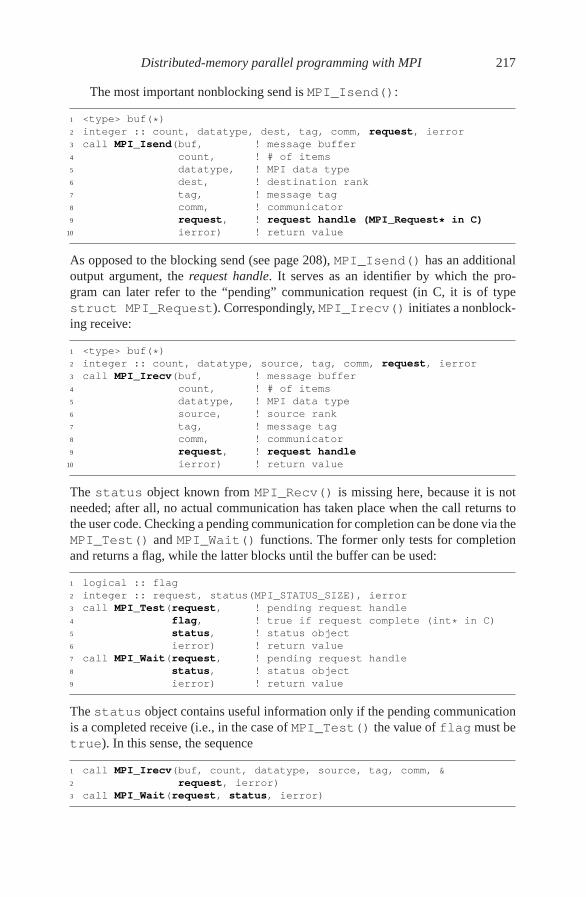
Distributed-memory parallel programming with MPI 217
The most important nonblocking send is MPI_Isend():
1 <type> buf(*)
2 integer :: count, datatype, dest, tag, comm, request, ierror
3 call MPI_Isend(buf, ! message buffer
4 count, ! # of items
5 datatype, ! MPI data type
6 dest, ! destination rank
7 tag, ! message tag
8 comm, ! communicator
9 request, ! request handle (MPI_Request* in C)
10 ierror) ! return value
As opposed to the blocking send (see page 208), MPI_Isend() has an additionaloutput argument, the request handle. It serves as an identifier by which the pro-gram can later refer to the “pending” communication request (in C, it is of typestruct MPI_Request). Correspondingly, MPI_Irecv() initiates a nonblock-ing receive:
1 <type> buf(*)
2 integer :: count, datatype, source, tag, comm, request, ierror
3 call MPI_Irecv(buf, ! message buffer
4 count, ! # of items
5 datatype, ! MPI data type
6 source, ! source rank
7 tag, ! message tag
8 comm, ! communicator
9 request, ! request handle
10 ierror) ! return value
The status object known from MPI_Recv() is missing here, because it is notneeded; after all, no actual communication has taken place when the call returns tothe user code. Checking a pending communication for completion can be done via theMPI_Test() and MPI_Wait() functions. The former only tests for completionand returns a flag, while the latter blocks until the buffer can be used:
1 logical :: flag
2 integer :: request, status(MPI_STATUS_SIZE), ierror
3 call MPI_Test(request, ! pending request handle
4 flag, ! true if request complete (int* in C)
5 status, ! status object
6 ierror) ! return value
7 call MPI_Wait(request, ! pending request handle
8 status, ! status object
9 ierror) ! return value
The status object contains useful information only if the pending communicationis a completed receive (i.e., in the case of MPI_Test() the value of flag must betrue). In this sense, the sequence
1 call MPI_Irecv(buf, count, datatype, source, tag, comm, &
2 request, ierror)
3 call MPI_Wait(request, status, ierror)

218 Introduction to High Performance Computing for Scientists and Engineers
is completely equivalent to a standard MPI_Recv().A potential problem with nonblocking MPI is that a compiler has no way to know
that MPI_Wait() can (and usually will) modify the contents of buf. Hence, in thefollowing code, the compiler may consider it legal to move the final statement in line3 before the call to MPI_Wait():
1 call MPI_Irecv(buf, ..., request, ...)
2 call MPI_Wait(request, status, ...)
3 buf(1) = buf(1) + 1
This will certainly lead to a race condition and the contents of buf may be wrong.The inherent connection between the MPI_Irecv() and MPI_Wait() calls, me-diated by the request handle, is invisible to the compiler, and the fact that buf is notcontained in the argument list of MPI_Wait() is sufficient to assume that the codemodification is legal. A simple way to avoid this situation is to put the variable (orbuffer) into a COMMON block, so that potentially all subroutines may modify it. Seethe MPI standard [P15] for alternatives.
Multiple requests can be pending at any time, which is another great advantageof nonblocking communication. Sometimes a group of requests belongs together insome respect, and one would like to check not one, but any one, any number, or allof them for completion. This can be done with suitable calls that are parameterizedwith an array of handles. As an example we choose the MPI_Waitall() routine:
1 integer :: count, requests(*)
2 integer :: statuses(MPI_STATUS_SIZE,*), ierror
3 call MPI_Waitall(count, ! number of requests
4 requests, ! request handle array
5 statuses, ! statuses array (MPI_Status* in C)
6 ierror) ! return value
This call returns only after all the pending requests have been completed. The statusobjects are available in array_of_statuses(:,:).
The integration example in Listing 9.3 can make use of nonblocking communi-cation by overlapping the local interval integration on rank 0 with receiving resultsfrom the other ranks. Unfortunately, collectives cannot be used here because thereare no nonblocking collectives in MPI. Listing 9.4 shows a possible solution. Thereduction operation has to be done manually (lines 33–35), as in the original code.Array sizes for the status and request arrays are not known at compile time, hencethose must be allocated dynamically, as well as separate receive buffers for all ranksexcept 0 (lines 11–13). The collection of partial results is performed with a singleMPI_Waitall() in line 32. Nothing needs to be changed on the nonroot ranks;MPI_Send() is sufficient to communicate the partial results (line 39).
Nonblocking communication provides an obvious way to overlap communica-tion, i.e., overhead, with useful work. The possible performance advantage, however,depends on many factors, and may even be nonexistent (see Section 10.4.3 for adiscussion). But even if there is no real overlap, multiple outstanding nonblockingrequests may improve performance because the MPI library can decide which ofthem gets serviced first.

Distributed-memory parallel programming with MPI 219
Listing 9.4: Program fragment for parallel integration in MPI, using nonblocking point-to-point communication.
1 integer, allocatable, dimension(:,:) :: statuses
2 integer, allocatable, dimension(:) :: requests
3 double precision, allocatable, dimension(:) :: tmp
4 call MPI_Comm_size(MPI_COMM_WORLD, size, ierror)
5 call MPI_Comm_rank(MPI_COMM_WORLD, rank, ierror)
6
7 ! integration limits
8 a=0.d0 ; b=2.d0 ; res=0.d0
9
10 if(rank.eq.0) then
11 allocate(statuses(MPI_STATUS_SIZE, size-1))
12 allocate(requests(size-1))
13 allocate(tmp(size-1))
14 ! pre-post nonblocking receives
15 do i=1,size-1
16 call MPI_Irecv(tmp(i), 1, MPI_DOUBLE_PRECISION, &
17 i, 0, MPI_COMM_WORLD, &
18 requests(i), ierror)
19 enddo
20 endif
21
22 ! limits for "me"
23 mya=a+rank*(b-a)/size
24 myb=mya+(b-a)/size
25
26 ! integrate f(x) over my own chunk - actual work
27 psum = integrate(mya,myb)
28
29 ! rank 0 collects partial results
30 if(rank.eq.0) then
31 res=psum
32 call MPI_Waitall(size-1, requests, statuses, ierror)
33 do i=1,size-1
34 res=res+tmp(i)
35 enddo
36 write (*,*) ’Result: ’,res
37 ! ranks != 0 send their results to rank 0
38 else
39 call MPI_Send(psum, 1, &
40 MPI_DOUBLE_PRECISION, 0, 0, &
41 MPI_COMM_WORLD,ierror)
42 endif

220 Introduction to High Performance Computing for Scientists and Engineers
Point-to-point CollectiveB
lock
ing MPI_Send()
MPI_Ssend()
MPI_Bsend()
MPI_Recv()
MPI_Barrier()
MPI_Bcast()
MPI_Scatter()/MPI_Gather()
MPI_Reduce()
MPI_Reduce_scatter()
MPI_Allreduce()
Non
blo
ckin
g
MPI_Isend()
MPI_Irecv()
MPI_Wait()/MPI_Test()MPI_Waitany()/
MPI_Testany()
MPI_Waitsome()/MPI_Testsome()
MPI_Waitall()/MPI_Testall()
N/A
Table 9.3: MPI’s communication modes and a nonexhaustive overview of the correspondingsubroutines.
Table 9.3 gives an overview of available communication modes in MPI, and themost important library functions.
9.2.5 Virtual topologies
We have outlined the principles of domain decomposition as an example for dataparallelism in Section 5.2.1. Using the MPI functions covered so far, it is entirelypossible to implement domain decomposition on distributed-memory parallel com-puters. However, setting up the process grid and keeping track of which ranks have toexchange halo data is nontrivial. Since domain decomposition is such an importantpattern, MPI contains some functionality to support this recurring task in the formof virtual topologies. These provide a convenient process naming scheme, whichfits the required communication pattern. Moreover, they potentially allow the MPI li-brary to optimize communications by employing knowledge about network topology.Although arbitrary graph topologies can be described with MPI, we restrict ourselvesto Cartesian topologies here.
As an example, assume there is a simulation that handles a big double precisionarray P(1:3000,1:4000) containing 3000×4000 = 1.2×10⁷ words. The simula-tion runs on 3×4 = 12 processes, across which the array is distributed “naturally,” i.e.,each process holds a chunk of size 1000×1000. Figure 9.6 shows a possible Carte-sian topology that reflects this situation: Each process can either be identified by itsrank or its Cartesian coordinates. It has a number of neighbors, which depends on

Distributed-memory parallel programming with MPI 221
0 (0,0)
2 (0,2)
4 (1,1)
5 (1,2)
3 (1,0) 6 (2,0) 9 (3,0)
10 (3,1)7 (2,1)
11 (3,2)8 (2,2)
1 (0,1)
Figure 9.6: Two-dimen-sional Cartesian topol-ogy: 12 processes forma 3×4 grid, which is pe-riodic in the second di-mension but not in thefirst. The mapping be-tween MPI ranks andCartesian coordinates isshown.
the grid’s dimensionality. In our example, the number of dimensions is two, whichleads to at most four neighbors per process. Boundary conditions on each dimensioncan be closed (cyclic) or open.
MPI can help with establishing the mapping between ranks and Cartesian coordi-nates in the process grid. First of all, a new communicator must be defined to whichthe chosen topology is “attached.” This is done via the MPI_Cart_create()
function:
1 integer :: comm_old, ndims, dims(*), comm_cart, ierror
2 logical :: periods(*), reorder
3 call MPI_Cart_create(comm_old, ! input communicator
4 ndims, ! number of dimensions
5 dims, ! # of processes in each dim.
6 periods, ! periodicity per dimension
7 reorder, ! true = allow rank reordering
8 comm_cart, ! new cartesian communicator
9 ierror) ! return value
It generates a new, “Cartesian” communicator comm_cart, which can be used laterto refer to the topology. The periods array specifies which Cartesian directions areperiodic, and the reorder parameter allows, if true, for rank reordering so that therank of a process in communicators comm_old and comm_cart may differ. TheMPI library may choose a different ordering by using its knowledge about networktopology and anticipating that next-neighbor communication is often dominant ina Cartesian topology. Of course, communication between any two processes is stillallowed in the Cartesian communicator.
There is no mention of the actual problem size (3000×4000) because it is entirelythe user’s job to care for data distribution. All MPI can do is keep track of the topol-ogy information. For the topology shown in Figure 9.6, MPI_Cart_create()could be called as follows:
1 call MPI_Cart_create(MPI_COMM_WORLD, ! standard communicator
2 2, ! two dimensions
3 (/ 4, 3 /), ! 4x3 grid
4 (/ .false., .true. /), ! open/periodic
5 .false., ! no rank reordering

222 Introduction to High Performance Computing for Scientists and Engineers
6 comm_cart, ! Cartesian communicator
7 ierror)
If the number of MPI processes is given, finding an “optimal” extension of the gridin each direction (as needed in the dims argument to MPI_Cart_create())requires some arithmetic, which can be offloaded to the MPI_Dims_create()function:
1 integer :: nnodes, ndims, dims(*), ierror
2 call MPI_Dims_create(nnodes, ! number of nodes in grid
3 ndims, ! number of Cartesian dimensions
4 dims, ! input: /=0 # nodes fixed in this dir.
5 ! ==0 # calculate # nodes
6 ! output: number of nodes each dir.
7 ierror)
The dims array is both an input and an output parameter: Each entry in dims cor-responds to a Cartesian dimension. A zero entry denotes a dimension for whichMPI_Dims_create() should calculate the number of processes, and a nonzeroentry specifies a fixed number of processes. Under those constraints, the functiondetermines a balanced distribution, with all ndims extensions as close together aspossible. This is optimal in terms of communication overhead only if the overallproblem grid is cubic. If this is not the case, the user is responsible for setting appro-priate constraints, since MPI has no way to know the grid geometry.
Two service functions are responsible for the translation between Cartesian pro-cess coordinates and an MPI rank. MPI_Cart_coords() calculates the Cartesiancoordinates for a given rank:
1 integer :: comm_cart, rank, maxdims, coords(*), ierror
2 call MPI_Cart_coords(comm_cart, ! Cartesian communicator
3 rank, ! process rank in comm_cart
4 maxdims, ! length of coords array
5 coords, ! return Cartesian coordinates
6 ierror)
(If rank reordering was allowed when producing comm_cart, a process should al-ways obtain its rank by calling MPI_Comm_rank(comm_cart,...) first.) Theoutput array coords contains the Cartesian coordinates belonging to the process ofthe specified rank.
This mapping function is needed whenever one deals with domain decomposi-tion. The first information a process will obtain from MPI is its rank in the Cartesiancommunicator. MPI_Cart_coords() is then required to determine the coordi-nates so the process can calculate, e.g., which subdomain it should work on. SeeSection 9.3 below for an example.
The reverse mapping, i.e., from Cartesian coordinates to an MPI rank, is per-formed by MPI_Cart_rank():
1 integer :: comm_cart, coords(*), rank, ierror
2 call MPI_Cart_rank(comm_cart, ! Cartesian communicator
3 coords, ! Cartesian process coordinates

Distributed-memory parallel programming with MPI 223
7 (2,1)1 (0,1)
6 (2,0)3 (1,0)0 (0,0)
2 (0,2) 5 (1,2) 8 (2,2)
4 (1,1) Figure 9.7: Example for the result ofMPI_Cart_shift() on a part ofthe Cartesian topology from Figure 9.6.Executed by rank 4 with direction=0and disp=−1, the function returnsrank_source=7 and rank_dest=1.
4 rank, ! return process rank in comm_cart
5 ierror)
Again, the return value in rank is only valid in the comm_cart communicator ifreordering was allowed.
A regular task with domain decomposition is to find out who the next neigh-bors of a certain process are along a certain Cartesian dimension. In principle onecould start from its Cartesian coordinates, offset one of them by one (accounting foropen or closed boundary conditions) and map the result back to an MPI rank viaMPI_Cart_rank(). The MPI_Cart_shift() function does it all in one step:
1 integer :: comm_cart, direction, disp, rank_source,
2 integer :: rank_dest, ierror
3 call MPI_Cart_shift(comm_cart, ! Cartesian communicator
4 direction, ! direction of shift (0..ndims-1)
5 disp, ! displacement
6 rank_source, ! return source rank
7 rank_dest, ! return destination rank
8 ierror)
The direction parameter specifies within which Cartesian dimension the shiftshould be performed, and disp determines the distance and direction (positive ornegative). rank_source and rank_dest return the “neighboring” ranks, accord-ing to the other arguments. Figure 9.7 shows an example for a shift along the negativefirst dimension, executed on rank 4 in the topology given in Figure 9.6. The sourceand destination neighbors are 7 and 1, respectively. If a neighbor does not exist be-cause it would extend beyond the grid’s boundary in a noncyclic dimension, the rankwill be returned as the special value MPI_PROC_NULL. Using MPI_PROC_NULLas a source or destination rank in any communication call is allowed and will effec-tively render the call a dummy statement — no actual communication will take place.This can simplify programming because the boundaries of the grid do not have to betreated in a special way (see Section 9.3 for an example).

224 Introduction to High Performance Computing for Scientists and Engineers
9.3 Example: MPI parallelization of a Jacobi solver
As a nontrivial example for virtual topologies and other MPI functionalities weuse a simple Jacobi solver (see Sections 3.3 and 6.2) in three dimensions. As opposedto parallelization with OpenMP, where inserting a couple of directives was sufficient,MPI parallelization by domain decomposition is much more complex.
9.3.1 MPI implementation
Although the basic algorithm was described in Section 5.2.1, we require somemore detail now. An annotated flowchart is shown in Figure 9.8. The central part isstill the sweep over all subdomains (step 3); this is where the computational effortgoes. However, each subdomain is handled by a different MPI process, which posestwo difficulties:
1. The convergence criterion is based on the maximum deviation between thecurrent and the next time step across all grid cells. This value can be easilyobtained for each subdomain separately, but a reduction is required to get aglobal maximum.
2. In order for the sweep over a subdomain to yield the correct results, appropriateboundary conditions must be implemented. This is no problem for cells thatactually neighbor real boundaries, but for cells adjacent to a domain cut, theboundary condition changes from sweep to sweep: It is formed by the cellsthat lie right across the cut, and those are not available directly because theyare owned by another MPI process. (With OpenMP, all data is always visibleby all threads, making access across “chunk boundaries” trivial.)
The first problem can be solved directly by an MPI_Allreduce() call after everyprocess has obtained the maximum deviation maxdelta in its own domain (step 4in Figure 9.8).
As for the second problem, so-called ghost or halo layers are used to store copiesof the boundary information from neighboring domains. Since only a single ghostlayer per subdomain is required per domain cut, no additional memory must be al-located because a boundary layer is needed anyway. (We will see below, however,that some supplementary arrays may be necessary for technical reasons.) Before aprocess sweeps over its subdomain, which involves updating the T = 1 array fromthe T = 0 data, the T = 0 boundary values from its neighbors are obtained via MPIand stored in the ghost cells (step 2 in Figure 9.8). In the following we will outlinethe central parts of the Fortran implementation of this algorithm. The full code canbe downloaded from the book’s Web site.2 For clarity, we will declare importantvariables with each code snippet.
2http://www.hpc.rrze.uni-erlangen.de/HPC4SE/

Distributed-memory parallel programming with MPI 225
Y
N
������
��������
������
��������
����
������
����
��
����
������
����
��
sweep
subdomains
calculate
deviation
global max
communicate
halo layers
END
initialize grid
and boundaries
< ε ?
exchange grids
maxdelta
MPI_MAX,...)
MPI_Allreduce(MPI_IN_PLACE,
maxdelta,...,
1
2
3
4
5
6
Figure 9.8: Flowchart for distributed-memory parallelization of the Jacobi algorithm. Hatchedcells are ghost layers, dark cells are already updated in the T = 1 grid, and light-colored cellsdenote T = 0 data. White cells are real boundaries of the overall grid, whereas black cells areunused.

226 Introduction to High Performance Computing for Scientists and Engineers
First the required parameters are read by rank zero from standard input (line 10in the following listing): problem size (spat_dim), possible presets for number ofprocesses (proc_dim), and periodicity (pbc_check), each for all dimensions.
1 logical, dimension(1:3) :: pbc_check
2 integer, dimension(1:3) :: spat_dim, proc_dim
3
4 call MPI_Comm_rank(MPI_COMM_WORLD, myid, ierr)
5 call MPI_Comm_size(MPI_COMM_WORLD, numprocs, ierr)
6
7 if(myid.eq.0) then
8 write(*,*) ’ spat_dim , proc_dim, PBC ? ’
9 do i=1,3
10 read(*,*) spat_dim(i), proc_dim(i), pbc_check(i)
11 enddo
12 endif
13
14 call MPI_Bcast(spat_dim , 3, MPI_INTEGER, 0, MPI_COMM_WORLD, ierr)
15 call MPI_Bcast(proc_dim , 3, MPI_INTEGER, 0, MPI_COMM_WORLD, ierr)
16 call MPI_Bcast(pbc_check, 3, MPI_LOGICAL, 0, MPI_COMM_WORLD, ierr)
Although many MPI implementations have options to allow the standard input ofrank zero to be seen by all processes, a portable MPI program cannot rely on thisfeature, and must broadcast the data (lines 14–16). After that, the Cartesian topologycan be set up using MPI_Dims_create() and MPI_Cart_create():
1 call MPI_Dims_create(numprocs, 3, proc_dim, ierr)
2
3 if(myid.eq.0) write(*,’(a,3(i3,x))’) ’Grid: ’, &
4 (proc_dim(i),i=1,3)
5
6 l_reorder = .true.
7 call MPI_Cart_create(MPI_COMM_WORLD, 3, proc_dim, pbc_check, &
8 l_reorder, GRID_COMM_WORLD, ierr)
9
10 if(GRID_COMM_WORLD .eq. MPI_COMM_NULL) goto 999
11
12 call MPI_Comm_rank(GRID_COMM_WORLD, myid_grid, ierr)
13 call MPI_Comm_size(GRID_COMM_WORLD, nump_grid, ierr)
Since rank reordering is allowed (line 6), the process rank must be obtained againusing MPI_Comm_rank() (line 12). Moreover, the new Cartesian communicatorGRID_COMM_WORLD may be of smaller size than MPI_COMM_WORLD. The “sur-plus” processes then receive a communicator value of MPI_COMM_NULL, and aresent into a barrier to wait for the whole parallel program to complete (line 10).
Now that the topology has been created, the local subdomains can be set up,including memory allocation:
1 integer, dimension(1:3) :: loca_dim, mycoord
2
3 call MPI_Cart_coords(GRID_COMM_WORLD, myid_grid, 3,
4 mycoord,ierr)
5
Distributed-memory parallel programming with MPI 227
6 do i=1,3
7 loca_dim(i) = spat_dim(i)/proc_dim(i)
8 if(mycoord(i) < mod(spat_dim(i),proc_dim(i))) then
9 local_dim(i) = loca_dim(i)+1
10 endif
11 enddo
12
13 iStart = 0 ; iEnd = loca_dim(3)+1
14 jStart = 0 ; jEnd = loca_dim(2)+1
15 kStart = 0 ; kEnd = loca_dim(1)+1
16
17 allocate(phi(iStart:iEnd, jStart:jEnd, kStart:kEnd,0:1))
Array mycoord is used to store a process’ Cartesian coordinates as acquired fromMPI_Cart_coords() in line 3. Array loca_dim holds the extensions of a pro-cess’ subdomain in the three dimensions. These numbers are calculated in lines 6–11.Memory allocation takes place in line 17, allowing for an additional layer in all di-rections, which is used for fixed boundaries or halo as needed. For brevity, we areomitting the initialization of the array and its outer grid boundaries here.
Point-to-point communication as used for the ghost layer exchange requires con-secutive message buffers. (Actually, the use of derived MPI data types would be anoption here, but this would go beyond the scope of this introduction.) However, onlythose boundary cells that are consecutive in the inner (i) dimension are also consecu-tive in memory. Whole layers in the i- j, i-k, and j-k planes are never consecutive, soan intermediate buffer must be used to gather boundary data to be communicated to aneighbor’s ghost layer. Sending each consecutive chunk as a separate message is outof the question, since this approach would flood the network with short messages,and latency has to be paid for every request (see Chapter 10 for more information onoptimizing MPI communication).
We use two intermediate buffers per process, one for sending and one for re-ceiving. Since the amount of halo data can be different along different Cartesiandirections, the size of the intermediate buffer must be chosen to accommodate thelargest possible halo:
1 integer, dimension(1:3) :: totmsgsize
2
3 ! j-k plane
4 totmsgsize(3) = loca_dim(1)*loca_dim(2)
5 MaxBufLen=max(MaxBufLen,totmsgsize(3))
6 ! i-k plane
7 totmsgsize(2) = loca_dim(1)*loca_dim(3)
8 MaxBufLen=max(MaxBufLen,totmsgsize(2))
9 ! i-j plane
10 totmsgsize(1) = loca_dim(2)*loca_dim(3)
11 MaxBufLen=max(MaxBufLen,totmsgsize(1))
12
13 allocate(fieldSend(1:MaxBufLen))
14 allocate(fieldRecv(1:MaxBufLen))
At the same time, the halo sizes for the three directions are stored in the integer arraytotmsgsize.

228 Introduction to High Performance Computing for Scientists and Engineers
Now we can start implementing the main iteration loop, whose length is the max-imum number of iterations (sweeps), ITERMAX:
1 t0=0 ; t1=1
2 tag = 0
3 do iter = 1, ITERMAX
4 do disp = -1, 1, 2
5 do dir = 1, 3
6
7 call MPI_Cart_shift(GRID_COMM_WORLD, (dir-1), &
8 disp, source, dest, ierr)
9
10 if(source /= MPI_PROC_NULL) then
11 call MPI_Irecv(fieldRecv(1), totmsgsize(dir), &
12 MPI_DOUBLE_PRECISION, source, &
13 tag, GRID_COMM_WORLD, req(1), ierr)
14 endif ! source exists
15
16 if(dest /= MPI_PROC_NULL) then
17 call CopySendBuf(phi(iStart, jStart, kStart, t0), &
18 iStart, iEnd, jStart, jEnd, kStart, kEnd, &
19 disp, dir, fieldSend, MaxBufLen)
20
21 call MPI_Send(fieldSend(1), totmsgsize(dir), &
22 MPI_DOUBLE_PRECISION, dest, tag, &
23 GRID_COMM_WORLD, ierr)
24 endif ! destination exists
25
26 if(source /= MPI_PROC_NULL) then
27 call MPI_Wait(req, status, ierr)
28
29 call CopyRecvBuf(phi(iStart, jStart, kStart, t0), &
30 iStart, iEnd, jStart, jEnd, kStart, kEnd, &
31 disp, dir, fieldRecv, MaxBufLen)
32 endif ! source exists
33
34 enddo ! dir
35 enddo ! disp
36
37 call Jacobi_sweep(loca_dim(1), loca_dim(2), loca_dim(3), &
38 phi(iStart, jStart, kStart, 0), t0, t1, &
39 maxdelta)
40
41 call MPI_Allreduce(MPI_IN_PLACE, maxdelta, 1, &
42 MPI_DOUBLE_PRECISION, &
43 MPI_MAX, 0, GRID_COMM_WORLD, ierr)
44 if(maxdelta<eps) exit
45 tmp=t0; t0=t1; t1=tmp
46 enddo ! iter
47
48 999 continue
Halos are exchanged in six steps, i.e., separately per positive and negative Carte-sian direction. This is parameterized by the loop variables disp and dir. In line 7,MPI_Cart_shift() is used to determine the communication neighbors along the

Distributed-memory parallel programming with MPI 229
��������
��������
������������
��������
��������
������������
����
����
������
��������
��������
������������
R
R
R
R
R
S
S
S
S
S
R
R
R
R
R
S
S
S
S
S
CopyRecvBuf()CopySendBuf()
MPI_Send() MPI_Wait()MPI_Irecv()/
Figure 9.9: Halo communication for the Jacobi solver (illustrated in two dimensions here)along one of the coordinate directions. Hatched cells are ghost layers, and cells labeled “R”(“S”) belong to the intermediate receive (send) buffer. The latter is being reused for all otherdirections. Note that halos are always provided for the grid that gets read (not written) in theupcoming sweep. Fixed boundary cells are omitted for clarity.
current direction (source and dest). If a subdomain is located at a grid boundary,and periodic boundary conditions are not in place, the neighbor will be reported tohave rank MPI_PROC_NULL. MPI calls using this rank as source or destination willreturn immediately. However, as the copying of halo data to and from the intermedi-ate buffers should be avoided for efficiency in this case, we also mask out any MPIcalls, keeping overhead to a minimum (lines 10, 16, and 26).
The communication pattern along a direction is actually a ring shift (or a lin-ear shift in case of open boundary conditions). The problems inherent to a ringshift with blocking point-to-point communication were discussed in Section 9.2.2.To avoid deadlocks, and possibly utilize the available network bandwidth to fullextent, a nonblocking receive is initiated before anything else (line 11). This datatransfer can potentially overlap with the subsequent halo copy to the intermediatesend buffer, done by the CopySendBuf() subroutine (line 17). After sending thehalo data (line 21) and waiting for completion of the previous nonblocking receive(line 27), CopyRecvBuf() finally copies the received halo data to the boundarylayer (line 29), which completes the communication cycle in one particular direc-tion. Figure 9.9 again illustrates this chain of events.
After the six halo shifts, the boundaries of the current grid phi(:,:,:,t0) areup to date, and a Jacobi sweep over the local subdomain is performed, which updatesphi(:,:,:,t1) from phi(:,:,:,t0) (line 37). The corresponding subrou-tine Jacobi_sweep() returns the maximum deviation between the previous andthe current time step for the subdomain (see Listing 6.5 for a possible implemen-tation in 2D). A subsequent MPI_Allreduce() (line 41) calculates the globalmaximum and makes it available on all processes, so that the decision whether toleave the iteration loop because convergence has been reached (line 44) can be madeon all ranks without further communication.

230 Introduction to High Performance Computing for Scientists and Engineers
1 2 3 4 6 8 12Number of processes/nodes
0
500
1000
1500P
erf
orm
ance [M
LU
Ps/s
ec]
GigE model (Tl = 50 µs, B = 170 MB/s)
1203 per process, InfiniBand
1203 per process, GigE
linear
1 2 3 4 6 8 12
1
1.2
1.4
1.6
GigE model
P(ideal)/P(GE)
(3,2
,2)
(2,2
,2)
(3,2
,1)
(2,2
,1)
(3,1
,1)
(2,1
,1)
Figure 9.10: Main panel: Weak scaling of the MPI-parallel 3D Jacobi code with problem size1203 per process on InfiniBand vs. Gigabit Ethernet networks. Only one process per node wasused. The domain decomposition topology (number of processes in each Cartesian direction)is indicated. The weak scaling performance model (crosses) can reproduce the GigE data well.Inset: Ratio between ideally scaled performance and Gigabit Ethernet performance vs. processcount. (Single-socket cluster based on Intel Xeon 3070 at 2.66 GHz, Intel MPI 3.2.)
9.3.2 Performance properties
The performance characteristics of the MPI-parallel Jacobi solver are typical formany domain decomposition codes. We distinguish between weak and strong scalingscenarios, as they show quite different features. All benchmarks were performed withtwo different interconnect networks (Intel MPI Version 3.2 over DDR InfiniBand vs.Gigabit Ethernet) on a commodity cluster with single-socket nodes based on IntelXeon 3070 processors at 2.66 GHz. A single process per node was used throughoutin order to get a simple scaling baseline and minimize intranode effects.
Weak scaling
In our performance models in Section 5.3.6 we have assumed that 3D domaindecomposition at weak scaling has constant communication overhead. This is, how-ever, not always true because a subdomain that is located at a grid boundary mayhave fewer halo faces to communicate. Fortunately, due to the inherent synchroniza-tion between subdomains, the overall runtime of the parallel program is dominatedby the slowest process, which is the one with the largest number of halo faces if allprocesses work on equally-sized subdomains. Hence, we can expect reasonably lin-ear scaling behavior even on slow (but nonblocking) networks, once there is at leastone subdomain that is surrounded by other subdomains in all Cartesian directions.

Distributed-memory parallel programming with MPI 231
The weak scaling data for a constant subdomain size of 1203 shown in Figure 9.10substantiates this conjecture:
Scalability on the InfiniBand network is close to perfect. For Gigabit Ethernet,communication still costs about 40% of overall runtime at large node counts, but thisfraction gets much smaller when running on fewer nodes. In fact, the performancegraph shows a peculiar “jagged” structure, with slight breakdowns at 4 and 8 pro-cesses. These breakdowns originate from fundamental changes in the communica-tion characteristics, which occur when the number of subdomains in any coordinatedirection changes from one to anything greater than one. At that point, internodecommunication along this axis sets in: Due to the periodic boundary conditions, ev-ery process always communicates in all directions, but if there is only one process in acertain direction, it exchanges halo data only with itself, using (fast) shared memory.The inset in Figure 9.10 indicates the ratio between ideal scaling and Gigabit Eth-ernet performance data. Clearly this ratio gets larger whenever a new direction getscut. This happens at the decompositions (2,1,1), (2,2,1), and (2,2,2), respectively,belonging to node counts of 2, 4, and 8. Between these points, the ratio is roughlyconstant, and since there are only three Cartesian directions, it can be expected to notexceed a value of ≈ 1.6 even for very large node counts, assuming that the networkis nonblocking. The same behavior can be observed with the InfiniBand data, but theeffect is much less pronounced due to the much larger (×10) bandwidth and lower(/20) latency. Note that, although we use a performance metric that is only relevantin the parallel part of the program, the considerations from Section 5.3.3 about “fake”weak scalability do not apply here; the single-CPU performance is on par with theexpectations from the STREAM benchmark (see Section 3.3).
The communication model described above is actually good enough for a quanti-tative description. We start with the assumption that the basic performance character-istics of a point-to-point message transfer can be described by a simple latency/band-width model along the lines of Figure 4.10. However, since sending and receivinghalo data on each MPI process can overlap for each of the six coordinate direc-tions, we must include a maximum bandwidth number for full-duplex data transferover a single link. The (half-duplex) PingPong benchmark is not accurate enoughto get a decent estimate for full-duplex bandwidth, even though most networks (in-cluding Ethernet) claim to support full-duplex. The Gigabit Ethernet network usedfor the Jacobi benchmark can deliver about 111 MBytes/sec for half-duplex and170 MBytes/sec for full-duplex communication, at a latency of 50 µs.
The subdomain size is the same regardless of the number of processes, so the rawcompute time Ts for all cell updates in a Jacobi sweep is also constant. Communi-cation time Tc, however, depends on the number and size of domain cuts that leadto internode communication, and we are assuming that copying to/from intermediatebuffers and communication of a process with itself come at no cost. Performance onN = NxNyNz processes for a particular overall problem size of L3N grid points (usingcubic subdomains of size L3) is thus
P(L,~N) =L3N
Ts(L)+Tc(L,~N), (9.1)

232 Introduction to High Performance Computing for Scientists and Engineers
where
Tc(L,~N) =c(L,~N)
B+ kTℓ . (9.2)
Here, c(L,~N) is the maximum bidirectional data volume transferred over a node’snetwork link, B is the full-duplex bandwidth, and k is the largest number (over allsubdomains) of coordinate directions in which the number of processes is greaterthan one. c(L,~N) can be derived from the Cartesian decomposition:
c(L,~N) = L2 · k ·2 ·8 (9.3)
For L = 120 this leads to the following numbers:
N (Nz,Ny,Nx) kc(L,~N)[MB]
P(L,~N)[MLUPs/sec]
NP1(L)
P(L,~N)
1 (1,1,1) 0 0.000 124 1.00
2 (2,1,1) 2 0.461 207 1.20
3 (3,1,1) 2 0.461 310 1.20
4 (2,2,1) 4 0.922 356 1.39
6 (3,2,1) 4 0.922 534 1.39
8 (2,2,2) 6 1.382 625 1.59
12 (3,2,2) 6 1.382 938 1.59
P1(L) is the measured single-processor performance for a domain of size L3. Theprediction for P(L,~N) can be seen in the third column, and the last column quantifiesthe “slowdown factor” compared to perfect scaling. Both are shown for comparisonwith the measured data in the main panel and inset of Figure 9.10, respectively. Themodel is clearly able to describe the performance features of weak scaling well,which is an indication that our general concept of the communication vs. computation“workflow” was correct. Note that we have deliberately chosen a small problem sizeto emphasize the role of communication, but the influence of latency is still minor.
Strong scaling
Figure 9.11 shows strong scaling performance data for periodic boundary condi-tions on two different problem sizes (1203 vs. 4803). There is a slight penalty for thesmaller size (about 10%) even with one processor, independent of the interconnect.For InfiniBand, the performance gap between the two problem sizes can mostly beattributed to the different subdomain sizes. The influence of communication on scal-ability is minor on this network for the node counts considered. On Gigabit Ethernet,however, the smaller problem scales significantly worse because the ratio of halodata volume (and latency overhead) to useful work becomes so large at larger nodecounts that communication dominates the performance on this slow network. Thetypical “jagged” pattern in the scaling curve is superimposed by the communicationvolume changing whenever the number of processes changes. A simple predictivemodel as with weak scaling is not sufficient here; especially with small grids, there is

Distributed-memory parallel programming with MPI 233
1 2 3 4 6 8 12Number of processes/nodes
0
500
1000
1500
Pe
rfo
rma
nce
[M
LU
Ps/s
ec]
1203 ideal
1203 InfiniBand
1203 GigE
4803 ideal
4803 InfiniBand
4803 GigE
Figure 9.11: Strong sca-ling of the MPI-paral-lel 3D Jacobi code withproblem size 1203 (cir-cles) and 4803 (squares)on IB (filled symbols)vs. GigE (open sym-bols) networks. Only oneprocess per node wasused. (Same system andMPI topology as in Fig-ure 9.10.)
a strong dependence of single-process performance on the subdomain size, and intra-node communication processes (halo exchange) become important. See Problem 9.4and Section 10.4.1 for some more discussion.
Note that this analysis must be refined when dealing with multiple MPI processesper node, as is customary with current parallel systems (see Section 4.4). Especiallyon fast networks, intranode communication characteristics play a central role (seeSection 10.5 for details). Additionally, copying of halo data to and from intermediatebuffers within a process cannot be neglected.
Problems
For solutions see page 304 ff.
9.1 Shifts and deadlocks. Does the remedy for the deadlock problem with ringshifts as shown in Figure 9.2 (exchanging send/receive order) also work if thenumber of processes is odd?
What happens if the chain is open, i.e., if rank 0 does not communicate withthe highest-numbered rank? Does the reordering of sends and receives make adifference in this case?
9.2 Deadlocks and nonblocking MPI. In order to avoid deadlocks, we used non-blocking receives for halo exchange in the MPI-parallel Jacobi code (Sec-tion 9.3.1). An MPI implementation is actually not required to support overlap-ping of communication and computation; MPI progress, i.e., real data transfer,might happen only if MPI library code is executed. Under such conditions, isit still guaranteed that deadlocks cannot occur? Consult the MPI standard if indoubt.

234 Introduction to High Performance Computing for Scientists and Engineers
9.3 Open boundary conditions. The performance model for weak scaling of the Ja-cobi code in Section 9.3.2 assumed periodic boundary conditions. How wouldthe model change for open (Dirichlet-type) boundaries? Would there still beplateaus in the inset of Figure 9.10? What would happen when going from 12to 16 processes? What is the minimum number of processes for which the ratiobetween ideal and real performance reaches its maximum?
9.4 A performance model for strong scaling of the parallel Jacobi code. As men-tioned in Section 9.3.2, a performance model that accurately predicts the strongscaling behavior of the MPI-parallel Jacobi code is more involved than forweak scaling. Especially the dependence of the single-process performanceon the subdomain size is hard to predict since it depends on many factors(pipelining effects, prefetching, spatial blocking strategy, copying to interme-diate buffers, etc.). This was no problem for weak scaling because of the con-stant subdomain size. Nevertheless one could try to establish a partly “phe-nomenological” model by measuring single-process performance for all sub-domain sizes that appear in the parallel run, and base a prediction for parallelperformance on those baselines. What else would you consider to be requiredenhancements to the weak scaling model? Take into account that Ts becomessmaller and smaller as N grows, and that halo exchange is not the only inter-node communication that is going on.
9.5 MPI correctness. Is the following MPI program fragment correct? Assume thatonly two processes are running, and that my_rank contains the rank of eachprocess.
1 if(my_rank.eq.0) then
2 call MPI_Bcast(buf1, count, type, 0, comm, ierr)
3 call MPI_Send(buf2, count, type, 1, tag, comm, ierr)
4 else
5 call MPI_Recv(buf2, count, type, 0, tag, comm, status, ierr)
6 call MPI_Bcast(buf1, count, type, 0, comm, ierr)
7 endif
(This example is taken from the MPI 2.2 standard document [P15].)

Chapter 10
Efficient MPI programming
Substantial optimization potential is hidden in many MPI codes. After making surethat single-process performance is close to optimal by applying the methods de-scribed in Chapters 2 and 3, an MPI program should always be benchmarked forperformance and scalability to unveil any problems connected to parallelization.Some of those are not related to message passing or MPI itself but emerge fromwell-known general issues such as serial execution (Amdahl’s Law), load imbalance,unnecessary synchronization, and other effects that impact all parallel programmingmodels. However, there are also very specific problems connected to MPI, and manyof them are caused by implicit but unjustified assumptions about distributed-memoryparallelization, or from over-optimistic notions regarding the cost and side effects ofcommunication. One should always keep in mind that, while MPI was designed toprovide portable and efficient message passing functionality, the performance of agiven code is not portable across platforms.
This chapter tries to sketch the most relevant guidelines for efficient MPI pro-gramming, which are, to varying degrees, beneficial on all platforms and MPI imple-mentations. Such an overview is necessarily incomplete, since every algorithm hasits peculiarities. As in previous chapters on optimization, we will start by a brief in-troduction to typical profiling tools that are able to detect parallel performance issuesin message-passing programs.
10.1 MPI performance tools
In contrast to serial programming, it is usually not possible to pinpoint the rootcauses of MPI performance problems by simple manual instrumentation. Several freeand commercial tools exist for advanced MPI profiling [T24, T25, T26, T27, T28].As a first step one usually tries to get a rough overview of how much time is spentin the MPI library in relation to application code, which functions dominate, andprobably what communication volume is involved. This kind of data can at least showwhether communication is a problem at all. IPM [T24] is a simple and low-overheadtool that is able to retrieve this information. Like most MPI profilers, IPM uses theMPI profiling interface, which is part of the standard [P15]. Each MPI function is atrivial wrapper around the actual function, whose name stars with “PMPI_.” Hence,a preloaded library or even the user code can intercept MPI calls and collect profilingdata. In case of IPM, it is sufficient to preload a dynamic library (or link with a static
235

236 Introduction to High Performance Computing for Scientists and Engineers
Figure 10.1: (See color insert after page 262.) IPM “communication balance” of a master-worker style parallel application. The complete runtime was about 38 seconds, which are spentalmost entirely inside MPI_Recv() on rank 0. The other ranks are very load imbalanced,spending between 10 and 50% of their time in a barrier.
version) and run the application. Information about data volumes (per process and perprocess pair), time spent in MPI calls, load imbalance, etc., is then accumulated overthe application’s runtime, and can be viewed in graphical form. Figure 10.1 showsthe “communication balance” graph of a master-worker application, as generated byIPM. Each bar corresponds to an MPI rank and shows how much time the processspends in the different MPI functions. It is important to compare those times to theoverall runtime of the program, because a barrier time of twenty seconds meansnothing if the program runs for hours. In this example, the runtime was 38 seconds.Rank 0 (the master) distributes work among the workers, so it spends most of itsruntime in MPI_Recv(), waiting for results. The workers are obviously quite loadimbalanced, and between 5 and 50% of their time is wasted waiting at barriers. Asmall change in parameters (reducing the size of the work packages) was able tocorrect this problem, and the resulting balance graph is shown in Figure 10.2. Overallruntime was reduced, quite expectedly, by about 25%.
Note that care must be taken when interpreting summary results that were takenover the complete runtime of an application. Essentially the same reservations applyas for global hardware performance counter information (see Section 2.1.2). IPMhas a small API that can collect information broken down into user-definable phases,but sometimes more detailed data is required. A functionality that more advancedtools support is the event timeline. An MPI program can be decomposed into veryspecific events (message send/receive, collective operations, blocking wait,. . . ), andthose can easily be visualized in a timeline display. Figure 10.3 is a screenshot from“Intel Trace Analyzer” [T26], a GUI application that allows browsing and analysis of

Efficient MPI programming 237
Figure 10.2: (See color insert after page 262.) IPM function profile of the same application asin Figure 10.1, with the load imbalance problem removed.
trace data written by an MPI program (the code must be linked to a special collectorlibrary before running). The top panel shows a zoomed view of a timeline from a codesimilar to the MPI-parallel Jacobi solver from Section 9.3.1. In this view, point-to-point messages are depicted by black lines, and bright lines denote collectives. Eachprocess is broken down along the time axis into MPI (bright) and user code (dark)parts. The runtime is clearly dominated by MPI communication in this example. Piecharts in the lower left panel summarize, for each process, what fraction of timeis spent with user code and MPI, respectively, making a possible load imbalanceevident (the code shown is well load balanced). Finally, in the lower right panel, thedata volume exchanged between pairs of processes can be read off for every possiblecombination. All this data can be displayed in more detail. For instance, all relevantparameters and properties of each message like its duration, data volume, source andtarget, etc., can be viewed separately. Graphs containing MPI contributions can bebroken down to show the separate MPI functions, and user code can be instrumentedso that different functions show up in the timeline and summary graphs.
Note that Intel Trace Analyzer is just one of many commercially and freely avail-able MPI profiling tools. While different tools may focus on different aspects, theyall serve the purpose of making the vast amount of data which is required to representthe performance properties of an MPI code easier to digest. Some tools put specialemphasis on large-scale systems, where looking at timelines of individual processesis useless; they try to provide a high-level overview and generate some automatictuning advice from the data. This is still a field of active, ongoing research [T29].
The effective use of MPI profiling tools requires a considerable amount of expe-rience, and there is no way a beginner can draw any use out of them without some

238 Introduction to High Performance Computing for Scientists and Engineers
Figure 10.3: (See color insert after page 262.) Intel Trace Analyzer timeline view (top), loadbalance analysis (left bottom) and communication summary (right bottom) for an MPI-parallelcode running on 12 nodes. Point-to-point (collective) messages are depicted by dark (bright)lines in the timeline view, while dark (light) boxes or pie slices denote executed application(MPI) code.
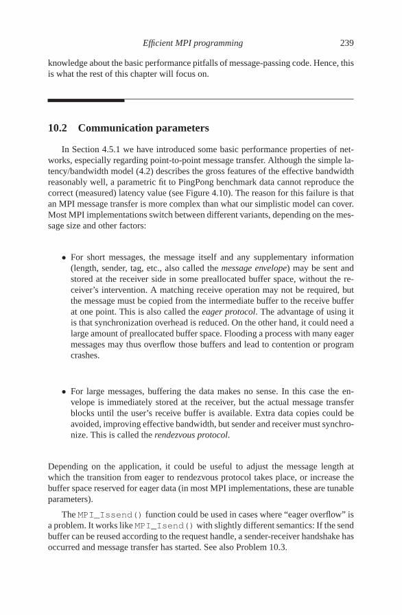
Efficient MPI programming 239
knowledge about the basic performance pitfalls of message-passing code. Hence, thisis what the rest of this chapter will focus on.
10.2 Communication parameters
In Section 4.5.1 we have introduced some basic performance properties of net-works, especially regarding point-to-point message transfer. Although the simple la-tency/bandwidth model (4.2) describes the gross features of the effective bandwidthreasonably well, a parametric fit to PingPong benchmark data cannot reproduce thecorrect (measured) latency value (see Figure 4.10). The reason for this failure is thatan MPI message transfer is more complex than what our simplistic model can cover.Most MPI implementations switch between different variants, depending on the mes-sage size and other factors:
• For short messages, the message itself and any supplementary information(length, sender, tag, etc., also called the message envelope) may be sent andstored at the receiver side in some preallocated buffer space, without the re-ceiver’s intervention. A matching receive operation may not be required, butthe message must be copied from the intermediate buffer to the receive bufferat one point. This is also called the eager protocol. The advantage of using itis that synchronization overhead is reduced. On the other hand, it could need alarge amount of preallocated buffer space. Flooding a process with many eagermessages may thus overflow those buffers and lead to contention or programcrashes.
• For large messages, buffering the data makes no sense. In this case the en-velope is immediately stored at the receiver, but the actual message transferblocks until the user’s receive buffer is available. Extra data copies could beavoided, improving effective bandwidth, but sender and receiver must synchro-nize. This is called the rendezvous protocol.
Depending on the application, it could be useful to adjust the message length atwhich the transition from eager to rendezvous protocol takes place, or increase thebuffer space reserved for eager data (in most MPI implementations, these are tunableparameters).
The MPI_Issend() function could be used in cases where “eager overflow” isa problem. It works like MPI_Isend()with slightly different semantics: If the sendbuffer can be reused according to the request handle, a sender-receiver handshake hasoccurred and message transfer has started. See also Problem 10.3.

240 Introduction to High Performance Computing for Scientists and Engineers
43
2
15
SendRecv
SendRecv
SendRecv
SendRecv
SendRecv
0 5
4
32
1
Figure 10.4: A linear shift communication pattern. Even with synchronous point-to-pointcommunication, a deadlock will not occur, but all message transfers will be serialized in theorder shown.
10.3 Synchronization, serialization, contention
This section elaborates on some performance problems that are not specific tomessage-passing, but may take special forms with MPI and hence deserve a detaileddiscussion.
10.3.1 Implicit serialization and synchronization
“Unintended” frequent synchronization or even serialization is a common phe-nomenon in parallel programming, and not limited to MPI. In Section 7.2.3 we havedemonstrated how careless use of OpenMP synchronization constructs can effec-tively serialize a parallel code. Similar pitfalls exist with MPI, and they are oftencaused by false assumptions about how messages are transferred.
The ring shift communication pattern, which was used in Section 9.2.2 to illus-trate the danger of creating a deadlock with blocking, synchronous point-to-pointmessages, is a good example. If the chain is open so that the ring becomes a lin-
Figure 10.5: Timeline view of the linear shift (see Fig-ure 10.4) with blocking (but not synchronous) sends andblocking receives, using eager delivery. Message trans-missions can overlap, making use of a nonblocking net-work. Eager delivery allows a send to end before the cor-responding receive is posted.
time
Rank
4
5
3
2
0
1
Recv
Recv
Recv
Recv
Recv
Recv
Send
Send
Send
Send
Send

Efficient MPI programming 241
Rank
4
5
3
2
0
1
Recv
RecvSend
Recv
Recv
Recv
Send
Send
Send
Send
Figure 10.6: Timeline view of thelinear shift (see Figure 10.4) withblocking synchronous sends andblocking receives, using eager de-livery. The message transfers (ar-rows) might overlap perfectly, buta send can only finish just after itsmatching receive is posted.
ear shift pattern, but sends and receives are performed on the processes in the ordershown in Figure 10.4, there will be no deadlock: Process 5 posts a receive, whichmatches the send on process 4. After that send has finished, process 4 can post its re-ceive, etc. Assuming the parameters are such that MPI_Send() is not synchronous,and “eager delivery” (see Section 10.2) can be used, a typical timeline graph, similarto what MPI performance tools would display, is depicted in Figure 10.5. Messagetransfers can overlap if the network is nonblocking, and since all send operationsterminate early (i.e., as soon as the blocking semantics is fulfilled), most of the timeis spent receiving data (note that there is no indication of where exactly the data is— it could be anywhere on its way from sender to receiver, depending on the imple-mentation).
There is, however, a severe performance problem with this pattern. If the messageparameters, first and foremost its length, are such that MPI_Send() is actuallyexecuted as MPI_Ssend(), the particular semantics of synchronous send must beobserved: MPI_Ssend() does not return to the user code before a matching receiveis posted on the target. This does not mean that MPI_Ssend() blocks until themessage has been fully transmitted and arrived in the receive buffer. Hence, a sendand its matching receive may overlap just by a small amount, which provides atleast some parallel use of the network but also incurs some performance penalty (seeFigure 10.6 for a timeline graph). A necessary prerequisite for this to work is thatmessage delivery still follows the eager protocol: If the conditions for eager deliveryare fulfilled, the data has “left” the send buffer (in terms of blocking semantics)already before the receive operation was posted, so it is safe even for a synchronoussend to terminate upon receiving some acknowledgment from the other side.
When the messages are transmitted according to the rendezvous protocol, thesituation gets worse. Buffering is impossible here, so sender and receiver must syn-chronize in a way that ensures full end-to-end delivery of the data. In our example,the five messages will be transmitted in serial, one after the other, because no pro-cess can finish its send operation until the next process down the chain has finishedits receive. The further down the chain a process is located, the longer its own syn-

242 Introduction to High Performance Computing for Scientists and Engineers
Rank
4
5
3
2
0
1
Recv
Send Recv
Recv
Recv
Recv
Send
Send
Send
Send
Figure 10.7: Timeline view of the linear shift (see Figure 10.4) with blocking sends and block-ing receives, using the rendezvous protocol. The messages (arrows) are transmitted in serialbecause buffering is ruled out.
chronous send operation will block, and there is no potential for overlap. Figure 10.7illustrates this with a timeline graph.
Implicit serialization should be avoided because it is not only a source of addi-tional communication overhead but can also lead to load imbalance, as shown above.Therefore, it is important to think about how (ring or linear) shifts, of which ghostlayer exchange is a variant, and similar patterns can be performed efficiently. Thebasic alternatives have already been described in Section 9.2.2:
• Change the order of sends and receives on, e.g., all odd-numbered processes(See Figure 10.8). Pairs of processes can then exchange messages in parallel,using at least part of the available network capacity.
• Use nonblocking functions as shown with the parallel Jacobi solver in Sec-tion 9.3. Nonblocking functions have the additional benefit that multiple out-standing communications can be handled by the MPI library in a (hopefully)optimal order. Moreover they provide at least an opportunity for truly asyn-chronous communication, where auxiliary threads and/or hardware mecha-nisms transfer data even while a process is executing user code. Note thatthis mode of operation must be regarded as an optimization provided by theMPI implementation; the MPI standard intentionally avoids any specificationsabout asynchronous transfers.
• Use blocking point-to-point functions that are guaranteed not to deadlock, re-gardless of message size, notably MPI_Sendrecv() (see also Problem 10.7)or MPI_Sendrecv_replace(). Internally, these calls are often imple-mented as combinations of nonblocking calls and MPI_Wait(), so they areactually convenience functions.

Efficient MPI programming 243
Rank
5
4
3
2
1
0
Recv
Send Recv
Recv Send
Send Recv
Recv Send
Send
Figure 10.8: Even if sends are synchronous and therendezvous protocol is used, exchanging the orderof sends and receives on all odd-numbered ranks ex-poses some parallelism in communication.
10.3.2 Contention
The simple latency/bandwidth communication model that we have used so far,together with the refinements regarding message delivery (see Section 10.2) can ex-plain a lot of effects, but it does not encompass contention effects. Here we want torestrict the discussion of contention to network connections; shared resources withina shared-memory multisocket multicore system like a compute node are ignored (see,e.g., Sections 1.4, 4.2, and 6.2 for more information on those issues). Assuming atypical hybrid (hierarchical) parallel computer design as discussed in Section 4.4,network contention occurs on two levels:
• Multiple threads or processes on a node may issue communication requests toother nodes. If bandwidth does not scale to multiple connections, the availablebandwidth per connection will go down. This is very common with commoditysystems, which often have only a single network interface available for MPIcommunication (and sometimes even I/O to remote file systems). On thesemachines, a single thread can usually saturate the network interface. However,there are also parallel computers where multiple connections are required tomake full use of the available network bandwidth [O69].
• The network topology may not be fully nonblocking, i.e., the bisection band-width (see Section 4.5.1) may be lower than the product of the number of nodesand the single-connection bandwidth. This is common with, e.g., cubic meshnetworks or fat trees that are not fully nonblocking.
• Even if bisection bandwidth is optimal, static routing can lead to contentionfor certain communication patterns (see Figure 4.17 in Section 4.5.3). In thelatter case, changing the network fabric’s routing tables (if possible) may bean option if performance should be optimized for a single application with acertain, well-defined communication scheme [O57].
In general, contention of some kind is hardly avoidable in current parallel systemsif message passing is used in any but the most trivial ways. An actual impact on

244 Introduction to High Performance Computing for Scientists and Engineers
application performance will of course only be visible if communication representsa measurable part of runtime.
Note that there are communication patterns that are especially prone to causingcontention, like all-to-all message transmission where every process sends to everyother process; MPI’s MPI_Alltoall() function is a special form of this. It is tobe expected that the communication performance for all-to-all patterns on massivelyparallel architectures will continue to decline in the years to come.
Any optimization that reduces communication overhead and message transfervolume (see Section 10.4) will most probably also reduce contention. Even if thereis no way to lessen the amount of message data, it may be possible to rearrangecommunication calls so that contention is minimized [A85].
10.4 Reducing communication overhead
10.4.1 Optimal domain decomposition
Domain decomposition is one of the most important implementations of dataparallelism. Most fluid dynamics and structural mechanics simulations are basedon domain decomposition and ghost layer exchange. We have demonstrated in Sec-tion 9.3.2 that the performance properties of a halo communication can be modeledquite accurately in simple cases, and that the division of the whole problem intosubdomains determines the communicated data volume, influencing performance ina crucial way. We are now going to shed some light on the question what it maycost (in terms of overhead) to choose a “wrong” decomposition, elaborating on theconsiderations leading to the performance models for the parallel Jacobi solver inSection 9.3.2.
Minimizing interdomain surface area
Figure 10.9 shows different possibilities for the decomposition of a cubic domainof size L3 into N subdomains with strong scaling. Depending on whether the domaincuts are performed in one, two, or all three dimensions (top to bottom), the numberof elements that must be communicated by one process with its neighbors, c(L,N),changes its dependence on N. The best behavior, i.e., the steepest decline, is achievedwith cubic subdomains (see also Problem 10.4). We are neglecting here that the pos-sible options for decomposition depend on the prime factors of N and the actualshape of the overall domain (which may not be cubic). The MPI_Dims_create()function tries, by default, to make the subdomains “as cubic as possible,” under theassumption that the complete domain is cubic. As a result, although much easier toimplement, “slab” subdomains should not be used in general because they incur amuch larger and, more importantly, N-independent overhead as compared to pole-shaped or cubic ones. A constant cost of communication per subdomain will greatlyharm strong scalability because performance saturates at a lower level, determinedby the message size (i.e., the slab area) instead of the latency (see Eq. 5.27).

Efficient MPI programming 245
“Slabs”
c1d(L,N) = L ·L ·w ·2= 2wL2
“Poles”
c2d(L,N) = L · L√N·w · (2+2)
= 4wL2N−1/2
“Cubes”
c3d(L,N) =L
3√
N· L
3√
N·w · (2+2+2)
= 6wL2N−2/3
Figure 10.9: 3D domain decomposition of a cubic domain of size L3 (strong scaling) andperiodic boundary conditions: Per-process communication volume c(L,N) for a single-sitedata volume w (in bytes) on N processes when cutting in one (top), two (middle), or all three(bottom) dimensions.
The negative power of N appearing in the halo volume expressions for pole- andcube-shaped subdomains will dampen the overhead, but still the surface-to-volumeratio will grow with N. Even worse, scaling up the number of processors at con-stant problem size “rides the PingPong curve” down towards smaller messages and,ultimately, into the latency-dominated regime (see Section 4.5.1). This has alreadybeen shown implicitly in our considerations on refined performance models (Sec-tion 5.3.6, especially Eq. 5.28) and “slow computing” (Section 5.3.8). Note that, inthe absence of overlap effects, each of the six halo communications is subject to la-tency; if latency dominates the overhead, “optimal” 3D decomposition may even becounterproductive because of the larger number of neighbors for each domain.
The communication volume per site (w) depends on the problem. For the simpleJacobi algorithm from Section 9.3, w = 16 (8 bytes each in positive and negative co-ordinate direction, using double precision floating-point numbers). If an algorithm re-quires higher-order derivatives or if there is some long-range interaction, w is larger.The same is true if one grid point is a more complicated data structure than just ascalar, as is the case with, e.g., lattice-Boltzmann algorithms [A86, A87]. See alsothe following sections.
246 Introduction to High Performance Computing for Scientists and Engineers
Figure 10.10: A typicaldefault mapping of MPIranks (numbers) to sub-domains (squares) andcluster nodes (letters) fora two-dimensional 4 ×8 periodic domain de-composition. Each nodehas 16 connections toother nodes. Intranodeconnections are omitted.
A
B
C
D24 25 26 27 28 29 30 31
16 17 18 19
8 9 10 11
0 1 2 3 4 5 6 7
12 13 14 15
20 21 22 23
Mapping issues
Modern parallel computers are inevitably of the hierarchical type. They all con-sist of shared-memory multiprocessor “nodes” coupled via some network (see Sec-tion 4.4). The simplest way to use this kind of hardware is to run one MPI processper core. Assuming that any point-to-point MPI communication between two coreslocated on the same node is much faster (in terms of bandwidth and latency) than be-tween cores on different nodes, it is clear that the mapping of computational subdo-mains to cores has a large impact on communication overhead. Ideally, this mappingshould be optimized by MPI_Cart_create() if rank reordering is allowed, butmost MPI implementations have no idea about the parallel machine’s topology.
As simple example serves to illustrate this point. The physical problem is a two-dimensional simulation on a 4×8 Cartesian process grid with periodic boundary con-ditions. Figure 10.10 depicts a typical “default” configuration on four nodes (A . . . D)with eight cores each (we are neglecting network topology and any possible nodesubstructure like cache groups, ccNUMA locality domains, etc.). Under the assump-tion that intranode connections come at low cost, the efficiency of next-neighborcommunication (e.g., ghost layer exchange) is determined by the maximum numberof internode connection per node. The mapping in Figure 10.10 leads to 16 suchconnections. The “communicating surface” of each node is larger than it needs tobe because the eight subdomains it is assigned to are lined up along one dimension.Choosing a less oblong arrangement as shown in Figure 10.11 will immediately re-duce the number of internode connections, to twelve in this case, and consequentlycut down network contention. Since the data volume per connection is still the same,this is equivalent to a 25% reduction in internode communication volume. In fact, nomapping can be found that leads to an even smaller overhead for this problem.
Up to now we have presupposed that the MPI subsystem assigns successive ranksto the same node when possible, i.e., filling one node before using the next. Al-though this may be a reasonable assumption on many parallel computers, it shouldby no means be taken for granted. In case of a round-robin, or cyclic distribution,where successive ranks are mapped to successive nodes, the “best” solution fromFigure 10.11 will be turned into the worst possible alternative: Figure 10.12 illus-trates that each node now has 32 internode connections.

Efficient MPI programming 247
B
D
A
C
16
23
24
31
1 3 5
17
18
19
20
21
22
25
26
27
28
29
30
0 2 4 6 8 10 12 14
15131197
Figure 10.11: A “per-fect” mapping of MPIranks and subdomains tonodes. Each node has12 connections to othernodes.
Similar considerations apply to other types of parallel systems, like architecturesbased on (hyper-)cubic mesh networks (see Section 4.5.4), on which next-neighborcommunication is often favored. If the Cartesian topology does not match the map-ping of MPI ranks to nodes, the resulting long-distance connections can result inpainfully slow communication, as measured by the capabilities of the network. Theactual influence on application performance may vary, of course. Any type of map-ping might be acceptable if the parallel program is not limited by communication atall. However, it is good to keep in mind that the default provided by the MPI environ-ment should not be trusted. MPI performance tools, as described in Section 10.1, canbe used to display the effective bandwidth of every single point-to-point connection,and thus identify possible mapping issues if the numbers do not match expectations.
So far we have neglected any intranode issues, assuming that MPI communica-tion between the cores of a node is “infinitely fast.” While it is true that intranodelatency is far smaller than what any existing network technology can provide, band-width is an entirely different matter, and different MPI implementations vary widelyin their intranode performance. See Section 10.5 for more information. In truly hy-brid programs, where each MPI process consists of several OpenMP threads, themapping problem becomes even more complex. See Section 11.3 for a detailed dis-cussion.
1
C
D
A A C
B DB
C
D
A A C
B DB
C
D
A A C
B DB
C
D
A A C
B DB
0 8
15
16
23
24
31
1
2
3
4
5
6
7 9
10
11
12
13
14
17
18
19
20
21
22
25
26
27
28
29
30
Figure 10.12: The samerank-to-subdomain map-ping as in Figure 10.11,but with ranks assignedto nodes in a “round-robin” way, i.e., succes-sive ranks run on differ-ent nodes. This leads to32 internode connectionsper node.
248 Introduction to High Performance Computing for Scientists and Engineers
10.4.2 Aggregating messages
If a parallel algorithm requires transmission of a lot of small messages betweenprocesses, communication becomes latency-bound because each message incurs la-tency. Hence, small messages should be aggregated into contiguous buffers and sentin larger chunks so that the latency penalty must only be paid once, and effectivecommunication bandwidth is as close as possible to the saturation region of the Ping-Pong graph (see Figure 4.10 in Section 4.5.1). Of course, this advantage pertains topoint-to-point and collective communication alike.
Aggregation will only pay off if the additional time for copying the messages toa contiguous buffer does not outweigh the latency penalty for separate sends, i.e., if
(m−1)Tℓ >mL
Bc, (10.1)
where m is the number of messages, L is the message length, and Bc is the bandwidthfor memory-to-memory copies. For simplicity we assume that all messages have thesame length, and that latency for memory copies is negligible. The actual advantagedepends on the raw network bandwidth Bn as well, because the ratio of serialized andaggregated communication times is
Ts
Ta=
Tℓ/L+B−1n
Tℓ/mL+B−1c +B−1
n. (10.2)
On a slow network, i.e., if B−1n is large compared to the other expressions in the
numerator and denominator, this ratio will be close to one and aggregation will notbe beneficial.
A typical application of message aggregation is the use of multilayer halos withstencil solvers: After multiple updates (sweeps) have been performed on a subdo-main, exchange of multiple halo layers in a single message can exploit the “PingPongride” to reduce the impact of latency. If this approach appears feasible for optimizingan existing code, appropriate performance models should be employed to estimatethe expected gain [O53, A88].
Message aggregation and derived datatypes
A typical case for message aggregation comes up when separate, i.e., noncontigu-ous data items must be transferred between processes, like a row of a (Fortran) matrixor a completely unconnected bunch of variables, possibly of different types. MPI pro-vides so-called derived datatypes, which support this functionality. The programmercan introduce new datatypes beyond the built-in ones (MPI_INTEGER etc.) and usethem in communication calls. There is a variety of choices for defining new types:Array-like with gaps, indexed arrays, n-dimensional subarrays of n-dimensional ar-rays, and even a collection of unconnected variables of different types scattered inmemory. The new type must first be defined using MPI_Type_XXXXX(), where“XXXXX” designates one of the variants as described above. The call returns the newtype as an integer (in Fortran) or in an MPI_Datatype structure (in C/C++). In

Efficient MPI programming 249
count
oldtype
blocklength
stride
Figure 10.13: Required parameters for MPI_Type_vector. Here blocklength=2,stride=5, and count=2.
order to use the type, it must be “committed” with MPI_Type_commit(). In casethe type is not needed any more, it can be “freed” using MPI_Type_free().
We demonstrate these facilities by defining the new type to represent one rowof a Fortran matrix. Since Fortran implements column major ordering with mul-tidimensional arrays (see Section 3.2), a matrix row is noncontiguous in memory,with chunks of one item separated by a constant stride. The appropriate MPI callto use for this is MPI_Type_vector(), whose main parameters are depicted inFigure 10.13. We use it to define a row of a double precision matrix of dimensionsXMAX×YMAX. Hence, count=YMAX, blocklength=1, stride=XMAX, and theold type is MPI_DOUBLE_PRECISION:
1 double precision, dimension(XMAX,YMAX) :: matrix
2 integer newtype ! new type
3
4 call MPI_Type_vector(YMAX, ! count
5 1, ! blocklength
6 XMAX, ! stride
7 MPI_DOUBLE_PRECISION, ! oldtype
8 newtype, ! new type
9 ierr)
10 call MPI_Type_commit(newtype, ierr) ! make usable
11 ...
12 call MPI_Send(matrix(5,1), ! send 5th row
13 1, ! sendcount=1
14 newtype,...) ! use like any type
15 ...
16 call MPI_Type_free(newtype,ierr) ! release type
In line 12 the type is used to send the 5th row of the matrix, with a count argu-ment of 1 to the MPI_Send() function (care must be taken when sending morethan one instance of such a type, because “gaps” at the end of a single instance areignored by default; consult the MPI standard for details). Datatypes for simplifyinghalo exchange on Cartesian topologies can be established in a similar way.
Although derived types are convenient to use, their performance implications areunclear, which is a good example for the rule that performance optimizations arenot portable across MPI implementations. The library could aggregate the parts of

250 Introduction to High Performance Computing for Scientists and Engineers
the new type into an internal contiguous buffer, but it could just as well send thepieces separately. Even if aggregation takes place, one cannot be sure whether itis done in the most efficient way; e.g., nontemporal stores could be beneficial forlarge data volume, or (if multiple threads per MPI process are available) copyingcould be multithreaded. In general, if communication of derived datatypes is crucialfor performance, one should not rely on the library’s efficiency but check whethermanual copying improves performance. If it does, this “performance bug” should bereported to the provider of the MPI library.
10.4.3 Nonblocking vs. asynchronous communication
Besides the efforts towards reducing communication overhead as described in thepreceding sections, a further chance for increasing efficiency of parallel programs isoverlapping communication and computation. Nonblocking point-to-point commu-nication seems to be the straightforward way to achieve this, and we have actuallymade (limited) use of it in the MPI-parallel Jacobi solver, where we have employedMPI_Irecv() to overlap halo receive with copying data to the send buffer andsending it (see Section 9.3). However, there was no concurrency between stencil up-dates (which comprise the actual “work”) and communication. A way to achieve thiswould be to perform those stencil updates first that form subdomain boundaries, be-cause they must be transmitted to the halo layers of neighboring subdomains. Afterthe update and copying to intermediate buffers, MPI_Isend() could be used tosend the data while the bulk stencil updates are done.
However, as mentioned earlier, one must strictly differentiate between nonblock-ing and truly asynchronous communication. Nonblocking semantics, according tothe MPI standard, merely implies that the message buffer cannot be used after thecall has returned from the MPI library; while certainly desirable, it is entirely up tothe implementation whether data transfer, i.e., MPI progress, takes place while usercode is being executed outside MPI.
Listing 10.1 shows a simple benchmark that can be used to determine whether anMPI library supports asynchronous communication. This code is to be executed byexactly two processors (we have omitted initialization code, etc.). The do_work()function executes some user code with a duration given by its parameter in seconds.In order to rule out contention effects, the function should perform operations that donot interfere with simultaneous memory transfers, like register-to-register arithmetic.The data size for MPI (count) was chosen so that the message transfer takes a con-siderable amount of time (tens of milliseconds) even on the most modern networks.If MPI_Irecv() triggers a truly asynchronous data transfer, the measured overalltime will stay constant with increasing delay until the delay equals the message trans-fer time. Beyond this point, there will be a linear rise in execution time. If, on theother hand, MPI progress occurs only inside the MPI library (which means, in thisexample, within MPI_Wait()), the time for data transfer and the time for executingdo_work() will always add up and there will be a linear rise of overall executiontime starting from zero delay. Figure 10.14 shows internode data (open symbols) forsome current parallel architectures and interconnects. Among those, only the Cray

Efficient MPI programming 251
Listing 10.1: Simple benchmark for evaluating the ability of the MPI library to perform asyn-chronous point-to-point communication.
1 double precision :: delay
2 integer :: count, req
3 count = 80000000
4 delay = 0.d0
5
6 do
7 call MPI_Barrier(MPI_COMM_WORLD, ierr)
8 if(rank.eq.0) then
9 t = MPI_Wtime()
10 call MPI_Irecv(buf, count, MPI_BYTE, 1, 0, &
11 MPI_COMM_WORLD, req, ierr)
12 call do_work(delay)
13 call MPI_Wait(req, status, ierr)
14 t = MPI_Wtime() - t
15 else
16 call MPI_Send(buf, count, MPI_BYTE, 0, 0, &
17 MPI_COMM_WORLD, ierr)
18 endif
19 write(*,*) ’Overall: ’,t,’ Delay: ’,delay
20 delay = delay + 1.d-2
21 if(delay.ge.2.d0) exit
22 enddo
XT line of massively parallel systems supports asynchronous internode MPI by de-fault (open diamonds). For the IBM Blue Gene/P system the default behavior is to usepolling for message progress, which rules out asynchronous transfer (open squares).However, interrupt-based progress can be activated on this machine [V116], enablingasynchronous message-passing (filled squares).
One should mention that the results could change if the do_work() functionexecutes memory-bound code, because the message transfer may interfere with theCPU’s use of memory bandwidth. However, this effect can only be significant if thenetwork bandwidth is large enough to become comparable to the aggregate memorybandwidth of a node, but that is not the case on today’s systems.
Although the selection of systems is by no means an exhaustive survey of currenttechnology, the result is representative. Within the whole spectrum from commod-ity clusters to expensive, custom-made supercomputers, there is hardly any supportfor asynchronous nonblocking transfers, although most computer systems do featurehardware facilities like DMA engines that would allow background communication.The situation is even worse for intranode message passing because dedicated hard-ware for memory-to-memory copies is rare. For the Cray XT4 this is demonstratedin Figure 10.14 (filled diamonds). Note that the pure communication time roughlymatches the time for the intranode case, although the machine’s network is not usedand MPI can employ shared-memory copying. This is because the MPI point-to-pointbandwidth for large messages is nearly identical for intranode and internode situa-

252 Introduction to High Performance Computing for Scientists and Engineers
0 0.05 0.1 0.15 0.2 0.25Delay time [s]
0
0.05
0.1
0.15
0.2
0.25
0.3
0.35
0.4O
vera
ll tim
e [s]
QDR-IB cluster, Intel MPI 3.2.2
QDR-IB cluster, OpenMPI 1.4.1, Isend
QDR-IB cluster, OpenMPI 1.4.1, Irecv
SGI Altix 3700 (NumaLink 3)
IBM Blue Gene/P (default)
IBM Blue Gene/P (interrupts)
Cray XT4
Cray XT4 intranode
Figure 10.14: Results from the MPI overlap benchmark on different architectures, intercon-nects and MPI versions. Among those, only the MPI library on a Cray XT4 (diamonds) andOpenMPI on an InfiniBand cluster (filled triangles) are capable of asynchronous transfersby default, OpenMPI allowing no overlap for nonblocking receives, however. With intranodecommunication, overlap is generally unavailable on the systems considered. On the IBM BlueGene/P system, asynchronous transfers can be enabled by activating interrupt-driven progress(filled squares) via setting DCMF_INTERRUPTS=1.
tions, a feature that is very common among hybrid parallel systems. See Section 10.5for a discussion.
The lesson is that one should not put too much optimization effort into utilizingasynchronous communication by means of nonblocking point-to-point calls, becauseit will only pay off in very few environments. This does not mean, however, that non-blocking MPI is useless; it is valuable for preventing deadlocks, reducing idle timesdue to synchronization overhead, and handling multiple outstanding communicationrequests efficiently. An example for the latter is the utilization of full-duplex transfersif send and receive operations are outstanding at the same time. In contrast to asyn-chronous transfers, full-duplex communication is supported by most interconnectsand MPI implementations today.
Overlapping communication with computation is still possible even without di-rect MPI support by dedicating a separate thread (OpenMP, or any other variant ofthreading) to handling MPI calls while other threads execute user code. This is avariant of hybrid programming, which will be discussed in Chapter 11.
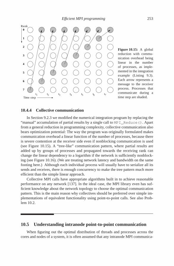
Efficient MPI programming 253
Time step
t t t t t t t2 3 4 5 6 71
0
1
2
3
4
5
6
7
Rank
Figure 10.15: A globalreduction with commu-nication overhead beinglinear in the numberof processes, as imple-mented in the integrationexample (Listing 9.3).Each arrow represents amessage to the receiverprocess. Processes thatcommunicate during atime step are shaded.
10.4.4 Collective communication
In Section 9.2.3 we modified the numerical integration program by replacing the“manual” accumulation of partial results by a single call to MPI_Reduce(). Apartfrom a general reduction in programming complexity, collective communication alsobears optimization potential: The way the program was originally formulated makescommunication overhead a linear function of the number of processes, because thereis severe contention at the receiver side even if nonblocking communication is used(see Figure 10.15). A “tree-like” communication pattern, where partial results areadded up by groups of processes and propagated towards the receiving rank canchange the linear dependency to a logarithm if the network is sufficiently nonblock-ing (see Figure 10.16). (We are treating network latency and bandwidth on the samefooting here.) Although each individual process will usually have to serialize all itssends and receives, there is enough concurrency to make the tree pattern much moreefficient than the simple linear approach.
Collective MPI calls have appropriate algorithms built in to achieve reasonableperformance on any network [137]. In the ideal case, the MPI library even has suf-ficient knowledge about the network topology to choose the optimal communicationpattern. This is the main reason why collectives should be preferred over simple im-plementations of equivalent functionality using point-to-point calls. See also Prob-lem 10.2.
10.5 Understanding intranode point-to-point communication
When figuring out the optimal distribution of threads and processes across thecores and nodes of a system, it is often assumed that any intranode MPI communica-

254 Introduction to High Performance Computing for Scientists and Engineers
Figure 10.16: With a tree-like, hierarchical reduction pat-tern, communication overhead is logarithmic in the num-ber of processes because communication during each timestep is concurrent. Time step
t t2 3
7
6
4
5
3
2
1
t1
0
Rank
tion is infinitely fast (see also Section 10.4.1 above). Surprisingly, this is not true ingeneral, especially with regard to bandwidth. Although even a single core can todaydraw a bandwidth of multiple GBytes/sec out of a chip’s memory interface, ineffi-cient intranode communication mechanisms used by the MPI implementation canharm performance dramatically. The simplest “bug” in this respect can arise whenthe MPI library is not aware of the fact that two communicating processes run on thesame shared-memory node. In this case, relatively slow network protocols are usedinstead of memory-to-memory copies. But even if the library does employ shared-memory communication where applicable, there is a spectrum of possible strategies:
• Nontemporal stores or cache line zero (see Section 1.3.1) may be used or not,probably depending on message and cache sizes. If a message is small andboth processes run in a cache group, using nontemporal stores is usually coun-terproductive because it generates additional memory traffic. However, if thereis no shared cache or the message is large, the data must be written to mainmemory anyway, and nontemporal stores avoid the write allocate that wouldotherwise be required.
• The data transfer may be “single-copy,” meaning that a simple block copy op-eration is sufficient to copy the message from the send buffer to the receivebuffer (implicitly implementing a synchronizing rendezvous protocol), or anintermediate (internal) buffer may be used. The latter strategy requires addi-tional copy operations, which can drastically diminish communication band-width if the network is fast.
• There may be hardware support for intranode memory-to-memory transfers.In situations where shared caches are unimportant for communication perfor-mance, using dedicated hardware facilities can result in superior point-to-pointbandwidth [138].

Efficient MPI programming 255
HT HT
Cro
ss
ba
r in
terc
on
ne
ct
HTHT
Memory Memory
Memory Memory
Memory Interface Memory Interface
Memory Interface
P
Memory Interface
P P P P P P P P
PPPPPPPL1D
L2
L1D
2MB L3
L2
L1D
L2
L1D
L2
L1D
L2
L1D
L2
L1D
L2
L1D
L2
2MB L3
L1D
L2L2
L1DL1D
L2L2
L1DL1D
L2L2
L1DL1D
L2L2
L1D
2MB L32MB L3
ASIC
ASIC
Figure 10.17: Two nodes of a Cray XT5 system. Dashed boxes denote AMD Opteron sockets,and there are two sockets (NUMA locality domains) per node. The crossbar interconnect isactually a 3D torus (mesh) network.
The behavior of MPI libraries with respect to above issues can sometimes be influ-enced by tunable parameters, but the rapid evolution of multicore processor architec-tures with complex cache hierarchies and system designs also makes it a subject ofintense development.
Again, the simple PingPong benchmark (see Section 4.5.1) from the IMB suitecan be used to fathom the properties of intranode MPI communication [O70, O71].As an outstanding example we use a Cray XT5 system. One XT5 node comprisestwo AMD Opteron chips with a 2 MB quad-core L3 group each. These nodes are con-nected via a 3D torus network (see Figure 10.17). Due to this structure one can expectthree different levels of point-to-point communication characteristics, depending onwhether message transfer occurs inside an L3 group (intranode intrasocket), betweencores on different sockets (intranode intersocket), or between different nodes (inter-node). (If a node had more than two ccNUMA locality domains, there would be evenmore variety.) Figure 10.18 shows internode and intranode PingPong data for thissystem. As expected, communication characteristics are quite different between in-ternode and intranode situations for small and intermediate-length messages. Twocores on the same socket can really benefit from the shared L3 cache, leading toa peak bandwidth of over 3 GBytes/sec. Surprisingly, the characteristics for inter-socket communication are very similar (dashed line), although there is no shared
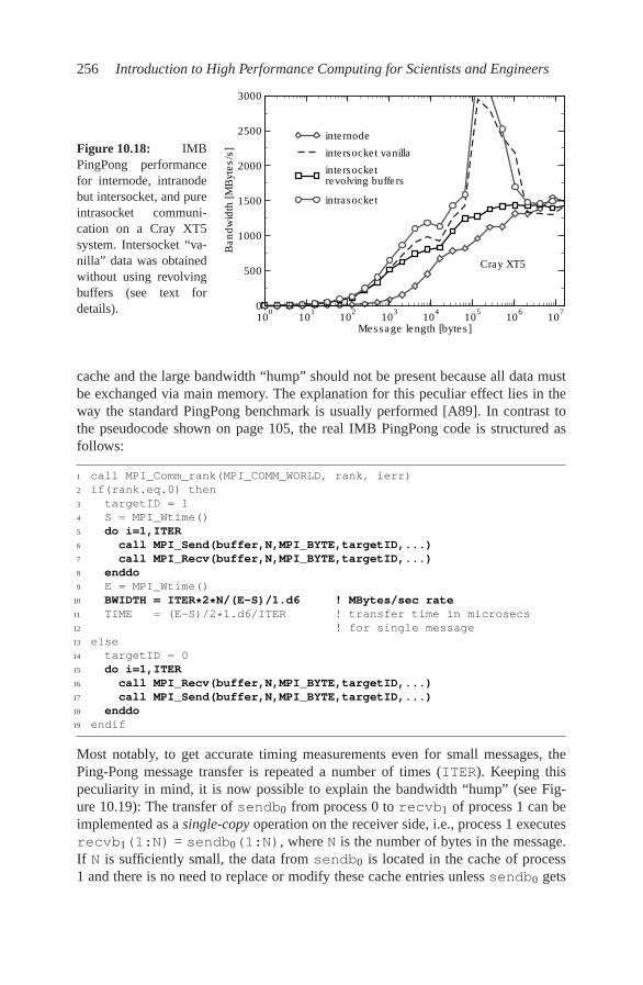
256 Introduction to High Performance Computing for Scientists and Engineers
Figure 10.18: IMBPingPong performancefor internode, intranodebut intersocket, and pureintrasocket communi-cation on a Cray XT5system. Intersocket “va-nilla” data was obtainedwithout using revolvingbuffers (see text fordetails).
100
101
102
103
104
105
106
107
Message length [bytes]
0
500
1000
1500
2000
2500
3000
Ba
nd
wid
th [
MB
yte
s/s
]
internode
intersocket vanilla
intersocket revolving buffers
intrasocket
Cray XT5
cache and the large bandwidth “hump” should not be present because all data mustbe exchanged via main memory. The explanation for this peculiar effect lies in theway the standard PingPong benchmark is usually performed [A89]. In contrast tothe pseudocode shown on page 105, the real IMB PingPong code is structured asfollows:
1 call MPI_Comm_rank(MPI_COMM_WORLD, rank, ierr)
2 if(rank.eq.0) then
3 targetID = 1
4 S = MPI_Wtime()
5 do i=1,ITER
6 call MPI_Send(buffer,N,MPI_BYTE,targetID,...)
7 call MPI_Recv(buffer,N,MPI_BYTE,targetID,...)
8 enddo
9 E = MPI_Wtime()
10 BWIDTH = ITER*2*N/(E-S)/1.d6 ! MBytes/sec rate
11 TIME = (E-S)/2*1.d6/ITER ! transfer time in microsecs
12 ! for single message
13 else
14 targetID = 0
15 do i=1,ITER
16 call MPI_Recv(buffer,N,MPI_BYTE,targetID,...)
17 call MPI_Send(buffer,N,MPI_BYTE,targetID,...)
18 enddo
19 endif
Most notably, to get accurate timing measurements even for small messages, thePing-Pong message transfer is repeated a number of times (ITER). Keeping thispeculiarity in mind, it is now possible to explain the bandwidth “hump” (see Fig-ure 10.19): The transfer of sendb0 from process 0 to recvb1 of process 1 can beimplemented as a single-copy operation on the receiver side, i.e., process 1 executesrecvb1(1:N) = sendb0(1:N), where N is the number of bytes in the message.If N is sufficiently small, the data from sendb0 is located in the cache of process1 and there is no need to replace or modify these cache entries unless sendb0 gets

Efficient MPI programming 257
P0 P1
C0 C1
M0 M1
����������
sendb 0sendb 1
sendb 0sendb 1
1recvb 0recvb
3
1
4
2
1. First ping: P1 copies sendb0 to recvb1,which resides in its cache.
2. First pong: P0 copies sendb1 to recvb0,which resides in its cache.
3. Second ping: P1 performs in-cache copy op-eration on its unmodified recvb1.
4. Second pong: P0 performs in-cache copy op-eration on its unmodified recvb0.
5. . . . Repeat steps 3 and 4, working in cache.
Figure 10.19: Chain of events for the standard MPI PingPong on shared-memory systemswhen the messages fit in the cache. C0 and C1 denote the caches of processors P0 and P1,respectively. M0 and M1 are the local memories of P0 and P1.
modified. However, the send buffers are not changed on either process in the loopkernel. Thus, after the first iteration the send buffers are located in the caches of thereceiving processes and in-cache copy operations occur in the subsequent iterationsinstead of data transfer through memory and the HyperTransport network.
There are two reasons for the performance drop at larger message sizes: First,the L3 cache (2 MB) is to small to hold both or at least one of the local receivebuffer and the remote send buffer. Second, the IMB is performed so that the numberof repetitions is decreased with increasing message size until only one iteration —which is the initial copy operation through the network — is done for large messages.
Real-world applications can obviously not make use of the “performance hump.”In order to evaluate the true potential of intranode communication for codes thatshould benefit from single-copy for large messages, one may add a second PingPongoperation in the inner iteration with arrays sendbi and recvbi interchanged (i.e.,sendbi is specified as the receive buffer with the second MPI_Recv() on processnumber i), the sending process i gains exclusive ownership of sendbi again. Anotheralternative is the use of “revolving buffers,” where a PingPong send/receive pair usesa small, sliding window out of a much larger memory region for send and receivebuffers, respectively. After each PingPong the window is shifted by its own size, sothat send and receive buffer locations in memory are constantly changing. If the sizeof the large array is chosen to be larger than any cache, it is guaranteed that all sendbuffers are actually evicted to memory at some point, even if a single message fits intocache and the MPI library uses single-copy transfers. The IMB benchmarks allow theuse of revolving buffers by a command-line option, and the resulting performancedata (squares in Figure 10.18) shows no overshooting for in-cache message sizes.
Interestingly, intranode and internode bandwidths meet at roughly the same as-ymptotic performance for large messages, refuting the widespread misconceptionthat intranode point-to-point communication is infinitely fast. This observation, al-

258 Introduction to High Performance Computing for Scientists and Engineers
Figure 10.20: Two nodes of aXeon 5160 dual-socket clustersystem with a DDR-InfiniBandinterconnect.
32k L1D32k L1D 32k L1D 32k L1D
32k L1D 32k L1D 32k L1D 32k L1D
Chipset
Memory
PPPP
4MB L24MB L2
Chipset
Memory
4MB L24MB L2
P P P P
infr
as
tru
ctu
re (
DD
R−
IB)
Ne
two
rk
PCIe/NIC
PCIe/NIC
though shown here for a specific system architecture and software environment, is al-most universal across many contemporary (hybrid) parallel systems, and especially“commodity” clusters. However, there is a large variation in the details, and sinceMPI libraries are continuously evolving, characteristics tend to change over time.In Figures 10.21 and 10.22 we show PingPong performance data on a cluster com-prised of dual-socket Intel Xeon 5160 nodes (see Figure 10.20), connected via DDR-InfiniBand. The only difference between the two graphs is the version number of theMPI library used (comparing Intel MPI 3.0 and 3.1). Details about the actual mod-ifications to the MPI implementation are undisclosed, but the observation of largeperformance variations between the two versions reveals that simple models aboutintranode communication are problematic and may lead to false conclusions.
At small message sizes, MPI communication is latency-dominated. For the sys-tems described above, the latencies measured by the IMB PingPong benchmark areshown in Table 10.1, together with asymptotic bandwidth numbers. Clearly, latencyis much smaller when both processes run on the same node (and smaller still if theyshare a cache). We must emphasize that these benchmarks can only give a roughimpression of intranode versus internode message passing issues. If multiple processpairs communicate concurrently (which is usually the case in real-world applica-tions), the situation gets much more complex. See Ref. [O72] for a more detailedanalysis in the context of hybrid MPI/OpenMP programming.
The most important conclusion that must be drawn from the bandwidth and la-tency characteristics shown above is that process-core affinity can play a major role

Efficient MPI programming 259
100
101
102
103
104
105
106
107
Message length [bytes]
0
500
1000
1500
2000
2500
3000
Ba
nd
wid
th [
MB
yte
s/s
]
internode
intersocketrevolving buffers
intrasocket
DDR-IB/PCIe 8x limit
Xeon 5160DDR-IB cluster
Figure 10.21: IMBPingPong performancefor internode, intranodebut intersocket, and pureintrasocket communica-tion on a Xeon 5160DDR-IB cluster, usingIntel MPI 3.0.
100
101
102
103
104
105
106
107
Message length [bytes]
0
500
1000
1500
2000
2500
3000
Ba
nd
wid
th [
MB
yte
s/s
]
internode
intersocket revolving buffers
intrasocket
DDR-IB/PCIe 8x limit
Xeon 5160DDR-IB cluster
Figure 10.22: The samebenchmark as in Fig-ure 10.21, but using IntelMPI 3.1. Intranode be-havior has changed sig-nificantly.
Latency [µs] Bandwidth [MBytes/sec]
XT5 Xeon-IB XT5 Xeon-IB
Mode MPT 3.1 IMPI 3.0 IMPI 3.1 MPT 3.1 IMPI 3.0 IMPI 3.1
internode 7.40 3.13 3.24 1500 1300 1300
intersocket 0.63 0.76 0.55 1400 750 1300
intrasocket 0.49 0.40 0.31 1500 1200 1100
Table 10.1: Measured latency and asymptotic bandwidth from the IMB PingPong benchmarkon a Cray XT5 and a commodity Xeon cluster with DDR-InifiniBand interconnect.

260 Introduction to High Performance Computing for Scientists and Engineers
for application performance on the “anisotropic” multisocket multicore systems thatare popular today (similar effects, though not directly related to communication, ap-pear in OpenMP programming, as shown in Sections 6.2 and 7.2.2). Mapping issuesas described in Section 10.4.1 are thus becoming relevant on the intranode topologylevel, too; for instance, given appropriate message sizes and an MPI code that mainlyuses next-neighbor communication, neighboring MPI ranks should be placed in thesame cache group. Of course, other factors like shared data paths to memory andNUMA constraints should be considered as well, and there is no general rule. Notealso that in strong scaling scenarios it is possible that one “rides down the PingPongcurve” towards a latency-driven regime with increasing processor count, possiblyrendering the performance assumptions useless that process/thread placement wasbased on for small numbers of processes (see also Problem 10.5).
Problems
For solutions see page 306 ff.
10.1 Reductions and contention. Comparing Figures 10.15 and 10.16, can you thinkof a network topology that would lead to the same performance for a reductionoperation in both cases? Assuming a fully nonblocking fat-tree network, whatcould be other factors that would prevent optimal performance with hierarchi-cal reductions?
10.2 Allreduce, optimized. We stated that MPI_Allreduce() is a combinationof MPI_Reduce() and MPI_Bcast(). While this is semantically correct,implementing MPI_Allreduce() in this way is very inefficient. How canit be done better?
10.3 Eager vs. rendezvous. Looking again at the overview on parallelization meth-ods in Section 5.2, what is a typical situation where using the “eager” messagetransfer protocol for MPI could have bad side effects? What are possible solu-tions?
10.4 Is cubic always optimal? In Section 10.4.1 we have shown that communicationoverhead for strong scaling due to halo exchange shows the most favorabledependence on N, the number of workers, if the domain is cut across all threecoordinate axes. Does this strategy always lead to minimum overhead?
10.5 Riding the PingPong curve. For strong scaling and cubic domain decomposi-tion with halo exchange as shown in Section 10.4.1, derive an expression forthe effective bandwidth Beff(N,L,w,Tℓ,B). Assume that a point-to-point mes-sage transfer can be described by the simple latency/bandwidth model (4.2),and that there is no overlap between communication in different directions andbetween computation and communication.

Efficient MPI programming 261
10.6 Nonblocking Jacobi revisited. In Section 9.3 we used a nonblocking receive toavoid deadlocks on halo exchange. However, exactly one nonblocking requestwas outstanding per process at any time. Can the code be reorganized to usemultiple outstanding requests? Are there any disadvantages?
10.7 Send and receive combined. MPI_Sendrecv() is a combination of a stan-dard send (MPI_Send()) and a standard receive (MPI_Recv()) in a singlecall:
1 <type> sendbuf(*), recvbuf(*)
2 integer :: sendcount, sendtype, dest, sendtag,
3 recvcount, recvtype, source, recvtag,
4 comm, status(MPI_STATUS_SIZE), ierror
5 call MPI_Sendrecv(sendbuf, ! send buffer
6 sendcount, ! # of items to send
7 sendtype, ! send data type
8 dest, ! destination rank
9 sendtag, ! tag for receive
10 recvbuf, ! receive buffer
11 recvcount, ! # of items to receive
12 recvtype, ! recv data type
13 source, ! source rank
14 recvtag, ! tag for send
15 status, ! status array for recv
16 comm, ! communicator
17 ierror) ! return value
How would you implement this function so that it is guaranteed not to deadlockif used for a ring shift communication pattern? Are there any other positive sideeffects to be expected?
10.8 Load balancing and domain decomposition. In 3D (cubic) domain decompo-sition with open (i.e., nontoroidal) boundary conditions, what are the implica-tions of communication overhead on load balance? Assume that the MPI com-munication properties are constant and isotropic throughout the parallel sys-tem, and that communication cannot be overlapped with computation. Wouldit make sense to enlarge the outermost subdomains in order to compensate fortheir reduced surface area?


Chapter 11
Hybrid parallelization with MPI andOpenMP
Large-scale parallel computers are nowadays exclusively of the distributed-memorytype at the overall system level but use shared-memory compute nodes as basic build-ing blocks. Even though these hybrid architectures have been in use for more than adecade, most parallel applications still take no notice of the hardware structure anduse pure MPI for parallelization. This is not a real surprise if one considers that theroots of most parallel applications, solvers and methods as well as the MPI libraryitself date back to times when all “big” machines were pure distributed-memorytypes, such as the famous Cray T3D/T3E MPP series. Later the existing MPI ap-plications and libraries were easy to port to shared-memory systems, and thus mosteffort was spent to improve MPI scalability. Moreover, application developers con-fided in the MPI library providers to deliver efficient MPI implementations, whichput the full capabilities of a shared-memory system to use for high-performance in-tranode message passing (see also Section 10.5 for some of the problems connectedwith intranode MPI). Pure MPI was hence implicitly assumed to be as efficient asa well-implemented hybrid MPI/OpenMP code using MPI for internode communi-cation and OpenMP for parallelization within the node. The experience with small-to moderately-sized shared-memory nodes (no more than two or four processors pernode) in recent years also helped to establish a general lore that a hybrid code canusually not outperform a pure MPI version for the same problem.
It is more than doubtful whether the attitude of running one MPI process percore is appropriate in the era of multicore processors. The parallelism within a singlechip will steadily increase, and the shared-memory nodes will have highly parallel,hierarchical, multicore multisocket structures. This section will shed some light onthis development and introduce basic guidelines for writing and running a good hy-brid code on this new class of shared-memory nodes. First, expected weaknesses andadvantages of hybrid OpenMP/MPI programming will be discussed. Turning to the“mapping problem,” we will point out that the performance of hybrid as well as pureMPI codes depends crucially on factors not directly connected to the programmingmodel, but to the association of threads and processes to cores. In addition, thereare several choices as to how exactly OpenMP threads and MPI processes can in-teract inside a node, which leaves significant room for improvement in most hybridapplications.
263

264 Introduction to High Performance Computing for Scientists and Engineers
11.1 Basic MPI/OpenMP programming models
The basic idea of a hybrid OpenMP/MPI programming model is to allow any MPIprocess to spawn a team of OpenMP threads in the same way as the master threaddoes in a pure OpenMP program. Thus, inserting OpenMP compiler directives into anexisting MPI code is a straightforward way to build a first hybrid parallel program.Following the guidelines of good OpenMP programming, compute intensive loopconstructs are the primary targets for OpenMP parallelization in a naïve hybrid code.Before launching the MPI processes one has to specify the maximum number ofOpenMP threads per MPI process in the same way as for a pure OpenMP program.At execution time each MPI process activates a team of threads (being the masterthread itself) whenever it encounters an OpenMP parallel region.
There is no automatic synchronization between the MPI processes for switchingfrom pure MPI to hybrid execution, i.e., at a given time some MPI processes may runin completely different OpenMP parallel regions, while other processes are in a pureMPI part of the program. Synchronization between MPI processes is still restrictedto the use of appropriate MPI calls.
We define two basic hybrid programming approaches [O69]: Vector mode andtask mode. These differ in the degree of interaction between MPI calls and OpenMPdirectives. Using the parallel 3D Jacobi solver as an example, the basic idea of bothapproaches will be briefly introduced in the following.
11.1.1 Vector mode implementation
In a vector mode implementation all MPI subroutines are called outside OpenMPparallel regions, i.e., in the “serial” part of the OpenMP code. A major advantage isthe ease of programming, since an existing pure MPI code can be turned hybrid justby adding OpenMP worksharing directives in front of the time-consuming loops andtaking care of proper NUMA placement (see Chapter 8). A pseudocode for a vectormode implementation of a 3D Jacobi solver core is shown in Listing 11.1. This looksvery similar to pure MPI parallelization as shown in Section 9.3, and indeed thereis no interference between the MPI layer and the OpenMP directives. Programmingfollows the guidelines for both paradigms independently. The vector mode strategy issimilar to programming parallel vector computers with MPI, where the inner layer ofparallelism is exploited by vectorization and multitrack pipelines. Typical exampleswhich may benefit from this mode are applications where the number of MPI pro-cesses is limited by problem-specific constraints. Exploiting an additional (lower)level of finer granularity by multithreading is then the only way to increase paral-lelism beyond the MPI limit [O70].

Hybrid parallelization with MPI and OpenMP 265
Listing 11.1: Pseudocode for a vector mode hybrid implementation of a 3D Jacobi solver.
1 do iteration=1,MAXITER
2 ...
3 !$OMP PARALLEL DO PRIVATE(..)
4 do k = 1,N
5 ! Standard 3D Jacobi iteration here
6 ! updating all cells
7 ...
8 enddo
9 !$OMP END PARALLEL DO
10
11 ! halo exchange
12 ...
13 do dir=i,j,k
14
15 call MPI_Irecv( halo data from neighbor in -dir direction )
16 call MPI_Isend( data to neighbor in +dir direction )
17
18 call MPI_Irecv( halo data from neighbor in +dir direction )
19 call MPI_Isend( data to neighbor in -dir direction )
20 enddo
21 call MPI_Waitall( )
22 enddo
11.1.2 Task mode implementation
The task mode is most general and allows any kind of MPI communication withinOpenMP parallel regions. Based on the thread safety requirements for the messagepassing library, the MPI standard defines three different levels of interference be-tween OpenMP and MPI (see Section 11.2 below). Before using task mode, the codemust check which of these levels is supported by the MPI library. Functional task de-composition and decoupling of communication and computation are two areas wheretask mode can be useful. As an example for the latter, a sketch of a task mode im-plementation of the 3D Jacobi solver core is shown in Listing 11.2. Here the masterthread is responsible for updating the boundary cells (lines 6–9), i.e., the surfacecells of the process-local subdomain, and communicates the updated values to theneighboring processes (lines 13–20). This can be done concurrently with the updateof all inner cells, which is performed by the remaining threads (lines 24–40). Af-ter a complete domain update, synchronization of all OpenMP threads within eachMPI process is required, while MPI synchronization only occurs indirectly betweennearest neighbors via halo exchange.
Task mode provides a high level of flexibility but blows up code size and in-creases coding complexity considerably. A major problem is that neither MPI norOpenMP has embedded mechanisms that directly support the task mode approach.Thus, one usually ends up with an MPI-style programming on the OpenMP level aswell. The different functional tasks need to be mapped to OpenMP thread IDs (cf.the if statement starting in line 5) and may operate in different parts of the code.

266 Introduction to High Performance Computing for Scientists and Engineers
Listing 11.2: Pseudocode for a task mode hybrid implementation of a 3D Jacobi solver.
1 !$OMP PARALLEL PRIVATE(iteration,threadID,k,j,i,...)
2 threadID = omp_get_thread_num()
3 do iteration=1,MAXITER
4 ...
5 if(threadID .eq. 0) then
6 ...
7 ! Standard 3D Jacobi iteration
8 ! updating BOUNDARY cells
9 ...
10 ! After updating BOUNDARY cells
11 ! do halo exchange
12
13 do dir=i,j,k
14 call MPI_Irecv( halo data from neighbor in -dir direction )
15 call MPI_Send( data to neighbor in +dir direction )
16 call MPI_Irecv( halo data from neighbor in +dir direction )
17 call MPI_Send( data to neighbor in -dir direction )
18 enddo
19
20 call MPI_Waitall( )
21
22 else ! not thread ID 0
23
24 ! Remaining threads perform
25 ! update of INNER cells 2,...,N-1
26 ! Distribute outer loop iterations manually:
27
28 chunksize = (N-2) / (omp_get_num_threads()-1) + 1
29 my_k_start = 2 + (threadID-1)*chunksize
30 my_k_end = 2 + (threadID-1+1)*chunksize-1
31 my_k_end = min(my_k_end, (N-2))
32
33 ! INNER cell updates
34 do k = my_k_start , my_k_end
35 do j = 2, (N-1)
36 do i = 2, (N-1)
37 ...
38 enddo
39 enddo
40 enddo
41 endif ! thread ID
42 !$OMP BARRIER
43 enddo
44 !$OMP END PARALLEL

Hybrid parallelization with MPI and OpenMP 267
Hence, the convenient OpenMP worksharing parallelization directives can no longerbe used. Workload has to be distributed manually among the threads updating theinner cells (lines 28–31). Note that so far only the simplest incarnation of the taskmode model has been presented. Depending on the thread level support of the MPIlibrary one may also issue MPI calls on all threads in an OpenMP parallel region,further impeding programmability. Finally, it must be emphasized that this hybridapproach prevents incremental hybrid parallelization, because substantial parts of anexisting MPI code need to be rewritten completely. It also severely complicates themaintainability of a pure MPI and a hybrid version in a single code.
11.1.3 Case study: Hybrid Jacobi solver
The MPI-parallel 3D Jacobi solver developed in Section 9.3 serves as a good ex-ample to evaluate potential benefits of hybrid programming for realistic applicationscenarios. To substantiate the discussion from the previous section, we now comparevector mode and a task mode implementations. Figure 11.1 shows performance datain MLUPs/sec for these two hybrid versions and the pure MPI variant using twodifferent standard networks (Gigabit Ethernet and DDR InfiniBand). In order to min-imize affinity and locality effects (cf. the extensive discussion in the next section),we choose the same single-socket dual-core cluster as in the pure MPI case study inSection 9.3.2. However, both cores per node are used throughout, which pushes theoverall performance over InfiniBand by 10–15% as compared to Figure 9.11 (for thesame large domain size of 4803). Since communication overhead is still almost neg-ligible when using InfiniBand, the pure MPI variant scales very well. It is no surprisethat no benefit from hybrid programming shows up for the InfiniBand network andall three variants (dashed lines) achieve the same performance level.
For communication over the GigE network the picture changes completely. Evenat low node counts the costs of data exchange substantially reduce parallel scalabil-ity for the pure MPI version, and there is a growing performance gap between GigEand InfiniBand. The vector mode does not help at all here, because computation andcommunication are still serialized; on the contrary, performance even degrades a bitsince only one core on a node is active during MPI communication. Overlapping ofcommunication and computation is efficiently possible in task mode, however. Par-allel scalability is considerably improved in this case and GigE performance comesvery close to the InfiniBand level.
This simple case study reveals the most important rule of hybrid programming:Consider going hybrid only if pure MPI scalability is not satisfactory. It does notmake sense to work hard on a hybrid implementation and try to be faster than aperfectly scaling MPI code.

268 Introduction to High Performance Computing for Scientists and Engineers
0 2 4 6 8 10 12 14 16# nodes
0
500
1000
1500
2000
2500P
erf
orm
an
ce
[M
LU
Ps/s
ec]
Perfect Scalability
Pure MPI (GigE)
Pure MPI (InfiniBand)
Vector Mode (GigE)
Vector Mode (InfiniBand)
Task Mode (GigE)
Task Mode (InfiniBand)
(2,2
,1)
(2,2
,2)
(4,2
,2)
(4,3
,2)
(4,4
,2)
(4,2
,2)
(3,2
,2)
(2,2
,2)
(2,2
,1)
(2,1
,1)
Figure 11.1: Pure MPI (circles) and hybrid (squares and diamonds) parallel performance ofa 3D Jacobi solver for strong scaling (problem size 4803) on the same single-socket dual-core cluster as in Figure 9.10, using DDR-InfiniBand (filled symbols) vs. Gigabit Ethernet(open symbols). The domain decomposition topology (number of processes in each Cartesiandirection) is indicated at each data point (below for hybrid and above for pure MPI). See textfor more details.
11.2 MPI taxonomy of thread interoperability
Moving from single-threaded to multithreaded execution is not an easy businessfrom a communication library perspective as well. A fully “thread safe” implementa-tion of an MPI library is a difficult undertaking. Providing shared coherent messagequeues or coherent internal message buffers are only two challenges to be namedhere. The most flexible case and thus the worst-case scenario for the MPI libraryis that MPI communication is allowed to happen on any thread at any time. SinceMPI may be implemented in environments with poor or no thread support, the MPIstandard currently (version 2.2) distinguishes four different levels of thread inter-operability, starting with no thread support at all (“MPI_THREAD_SINGLE”) andending with the most general case (“MPI_THREAD_MULTIPLE”):
• MPI_THREAD_SINGLE: Only one thread will execute.
• MPI_THREAD_FUNNELED: The process may be multithreaded, but only themain thread will make MPI calls.

Hybrid parallelization with MPI and OpenMP 269
(b) (c)(a)
MP
I
MP
I
MP
I
MP
I
MP
I
MP
I
MP
I
MP
I
MP
IM
PI
MP
I
MP
I
MP
I
Figure 11.2: Threading levels supported by MPI: (a) MPI_THREAD_FUNNELED, (b)MPI_THREAD_SERIALIZED, and (c) MPI_THREAD_MULTIPLE. The plain MPI modeMPI_THREAD_SINGLE is omitted. Typical communication patterns as permitted by the re-spective level of thread support are depicted for a single multithreaded MPI process with anumber of OpenMP threads.
• MPI_THREAD_SERIALIZED: The process may be multithreaded, and mul-tiple threads may make MPI calls, but only one at a time; MPI calls are notmade concurrently from two distinct threads.
• MPI_THREAD_MULTIPLE: Multiple threads may call MPI anytime, with norestrictions.
Every hybrid code should always check for the required level of threading supportusing the MPI_Init_thread() call. Figure 11.2 provides a schematic overviewof the different hybrid MPI/OpenMP modes allowed by MPI’s thread interoperabil-ity levels. Both hybrid implementations presented above for the parallel 3D Jacobisolver require MPI support for MPI_THREAD_FUNNELED since the master threadis the only one issuing MPI calls. The task mode version also provides first insightsinto the additional complications arising from multithreaded execution of MPI. Mostimportantly, MPI does not allow explicit addressing of different threads in a process.If there is a mandatory mapping between threads and MPI calls, the programmer hasto implement it. This can be done through the explicit use of OpenMP thread IDs andpotentially connecting them with different message tags (i.e., messages from differ-ent threads of the same MPI process are distinguished by unique MPI message tags).

270 Introduction to High Performance Computing for Scientists and Engineers
Another issue to be aware of is that synchronous MPI calls only block the callingthread, allowing the other threads of the same MPI process to execute, if possible.There are several more important guidelines to consider, in particular when fullyexploiting the MPI_THREAD_MULTIPLE capabilities. A thorough reading of thesection “MPI and Threads” in the MPI standard document [P15] is mandatory whenwriting multithreaded MPI code.
11.3 Hybrid decomposition and mapping
Once a hybrid OpenMP/MPI code has been implemented diligently and com-putational resources have been allocated, two important decisions need to be madebefore launching the application.
First one needs to select the number of OpenMP threads per MPI process and thenumber of MPI processes per node. Of course the capabilities of the shared mem-ory nodes at hand impose some limitations on this choice; e.g., the total number ofthreads per node should not exceed the number of cores in the compute node. Insome rare cases it might also be advantageous to either run a single thread per “vir-tual core” if the processor efficiently supports simultaneous multithreading (SMT,see Section 1.5) or to even use less threads than available cores, e.g., if memorybandwidth or cache size per thread is a bottleneck. Moreover, the physical problemto be solved and the underlying hardware architecture also strongly influence theoptimal choice of hybrid decomposition.
The mapping between MPI processes and OpenMP threads to sockets and coreswithin a compute node is another important decision. In this context the basic nodecharacteristics (number of sockets and number of cores per socket) can be used as afirst guideline, but even on rather simple two-socket compute nodes with multicoreprocessor chips there is a large parameter space in terms of decomposition and map-ping choices. In Figures 11.3–11.6 a representative subset is depicted for a clusterwith two standard two-socket quad-core ccNUMA nodes. We imply that the MPI li-brary supports the MPI_THREAD_FUNNELED level, where the master thread (t0) ofeach MPI process assumes a prominent position. This is valid for the two examplespresented above and reflects the approach implemented in many hybrid applications.
One MPI process per node
Considering the shared-memory feature only, one can simply assign a single MPIprocess to one node (m0,m1) and launch eight OpenMP threads (t0, . . . ,t7), i.e., oneper core (see Figure 11.3). There is a clear asymmetry between the hardware de-sign and the hybrid decomposition, which may show up in several performance-relevant issues. Synchronization of all threads is costly since it involves off-chipdata exchange and may become a major bottleneck when moving to multisocketand/or hexa-/octo-core designs [M41] (see Section 7.2.2 for how to estimate syn-chronization overhead in OpenMP). NUMA optimizations (see Chapter 8) need to

Hybrid parallelization with MPI and OpenMP 271
be considered when implementing the code; in particular, the typical locality andcontention issues can arise if the MPI process (running, e.g., in LD0) allocates sub-stantial message buffers. In addition the master thread may generate nonlocal dataaccesses when gathering data for MPI calls. Using less powerful cores, a single MPIprocess per node could also be insufficient to make full use of the latest interconnecttechnologies if the available internode bandwidth cannot be saturated by a single MPIprocess [O69]. The ease of launching the MPI processes and pinning the threads, aswell as the reduction of the number of MPI processes to a minimum are typical ad-vantages of this simple hybrid decomposition model.
One MPI process per socket
Assigning one multithreaded MPI process to each socket matches the node topol-ogy perfectly (see Figure 11.4). However, correctly launching the MPI processes andpinning the OpenMP threads in a blockwise fashion to the sockets requires due care.MPI communication may now happen both between sockets and between nodes con-currently, and appropriate scheduling of MPI calls should be considered in the appli-cation to overlap intersocket and internode communication [O72]. On the other hand,this mapping avoids ccNUMA data locality problems because each MPI process isrestricted to a single locality domain. Also the accessibility of a single shared cachefor all threads of each MPI process allows for fast thread synchronization and in-creases the probability of cache re-use between the threads. Note that this discussionneeds to be generalized to groups of cores with a shared outer-level cache: In the firstgeneration of Intel quad-core chips, groups of two cores shared an L2 cache while noL3 cache was available. For this chip architecture one should issue one MPI processper L2 cache group, i.e., two processes per socket.
A small modification of the mapping can easily emerge in a completely differentscenario without changing the number of MPI processes per node and the numberof OpenMP threads per process: If, e.g., a round-robin distribution of threads acrosssockets is chosen, one ends up in the situation shown in Figure 11.5. In each nodea single socket hosts two MPI processes, potentially allowing for very fast commu-nication between them via the shared cache. However, the threads of different MPIprocesses are interleaved on each socket, making efficient ccNUMA-aware program-ming a challenge by itself. Moreover, a completely different workload characteristicis assigned to the two sockets within the same node. All this is certainly close to aworst-case scenario in terms of thread synchronization and remote data access.
Multiple MPI processes per socket
Of course one can further increase the number of MPI Processes per node andcorrespondingly reduce the number of threads, ending up with two threads per MPIprocess. The choice of a block-wise distribution of the threads leads to the favorablescenario presented in Figure 11.6. While ccNUMA problems are of minor impor-tance here, MPI communication may show up on all potential levels: intrasocket,intersocket and internode. Thus, mapping the computational domains to the MPIprocesses in a way that minimizes access to the slowest communication path is a
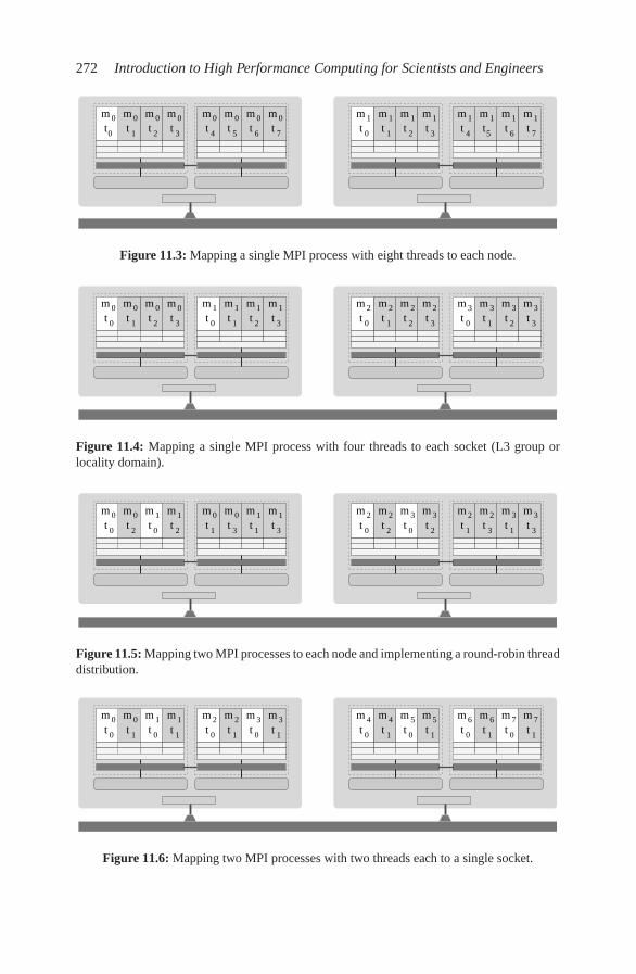
272 Introduction to High Performance Computing for Scientists and Engineers
t7
m0 m0
t4
t5
t6
m0 m0m0 m0
t3
t2
m0
t1
m0
t0
m1 m1
t3
t2
t7
m1 m1
t4
t5
m1
t1
m1
t6
1 m1
t
m
0
Figure 11.3: Mapping a single MPI process with eight threads to each node.
m2 m2
t3
t2
t3
m3 m3
t0
t1
m2
t1
m2
t2
3 m3
t
m
0
m0 m0
t3
t2
m0
t1
m0
t0
t3
m1 m1
t0
t1
t2
m1 m1
Figure 11.4: Mapping a single MPI process with four threads to each socket (L3 group orlocality domain).
m3 m3
t2
t0
t3
m2 m2
t1
t3
m2m2
t1
t2
3 m3
t
m
0t
2t
0
m0
t0
t3
m0 m0
t1
t3
m0
t2
t1
m1 m1m1 m1
Figure 11.5: Mapping two MPI processes to each node and implementing a round-robin threaddistribution.
m1 m1
t1
t0
m0
t1
m0
t0
t1
m2 m2
t0
t1
t0
m3 m3 m5 m5
t1
t0
t1
m6 m6
t0
t1
m4
t1
m4
t0
7 m7
t
m
0
Figure 11.6: Mapping two MPI processes with two threads each to a single socket.

Hybrid parallelization with MPI and OpenMP 273
potential optimization strategy. This decomposition approach can also be beneficialfor memory-intensive codes with limited MPI scalability. Often half of the threadsare already able to saturate the main memory bandwidth of a single socket and theuse of a multithreaded MPI process can add a bit to the performance gain from thesmaller number of MPI processes. Alternatively a functional decomposition can beemployed to explicitly hide MPI communication (see the task mode implementationof the Jacobi solver described above). It is evident that a number of different mappingstrategies is available for this decomposition as well. However, due to the symmetryarguments stressed several times above, the mapping in Figure 11.6 should generallyprovide best performance and thus be tested first.
Unfortunately, at the time of writing most MPI implementations only providevery poor support for defining different mapping strategies and pinning the threadscorrectly to the respective cores. If there is some support, it is usually restrictedto very specific combinations of MPI and compiler. Hence, the correct launch of ahybrid application is mostly the programmer’s responsibility, but indispensable fora profound performance study of hybrid codes. See Section 10.4.1 and Appendix Afor further information on mapping and affinity issues.
11.4 Potential benefits and drawbacks of hybrid programming
The hybrid parallel MPI/OpenMP approach is, for reasons mentioned earlier, stillrarely implemented to its full extent in parallel applications. Thus, it is not surprisingthat there is no complete theory available for whether a hybrid approach does payback the additional costs for code restructuring or designing a complete hybrid ap-plication from scratch. However, several potential fundamental advantages and draw-backs of the hybrid approach as compared to pure MPI have been identified so far.In the following we briefly summarize the most important ones. The impact of eachtopic below will most certainly depend on the specific application code or even onthe choice of input data. A careful investigation of those issues is mandatory if and
only if pure MPI scalability does not provide satisfactory parallel performance.
Improved rate of convergence
Many iterative solvers incorporate loop-carried data dependencies like, e.g., thewell-known lexicographical Gauss–Seidel scheme (see Section 6.3). Those depen-dencies are broken at boundary cells if standard domain decomposition is used forMPI parallelization. While the algorithm still converges to the correct steady-state so-lution, the rate of convergence typically drops with increasing number of subdomains(for strong scaling scenarios). Here a hybrid approach may help reduce the numberof subdomains and improve the rate of convergence. This was shown, e.g., for a CFDapplication with an implicit solver in [A90]: Launching only a single MPI processper node (computing on a single subdomain) and using OpenMP within the nodeimproves convergence in the parallel algorithm. This is clearly a case where parallel

274 Introduction to High Performance Computing for Scientists and Engineers
speedups or overall floating-point performance are the wrong metrics to quantify the“hybrid dividend.” Walltime to solution is the appropriate metric instead.
Re-use of data in shared caches
Using a shared-memory programming model for threads operating on a singleshared cache greatly extends the optimization opportunities: For iterative solvers withregular stencil dependencies like the Jacobi or Gauss–Seidel type, data loaded andmodified by a first thread can be read by another thread from cache and updated onceagain before being evicted to main memory. This trick leads to an efficient and nat-ural parallel temporal blocking, but requires a shared address space to avoid doublebuffering of in-cache data and redundant data copying (as would be enforced by apure MPI implementation) [O52, O53, O63]. Hybrid parallelization is mandatory toimplement such alternative multicore aware strategies in large-scale parallel codes.
Exploiting additional levels of parallelism
Many computational tasks provide a problem-immanent coarse-grained paral-lel level. One prominent example are some of the multizone NAS parallel bench-marks, where only a rather small number of zones are available for MPI paralleliza-tion (from a few dozens up to 256) and additional parallel levels can be exploitedby multithreaded execution of the MPI process [O70]. Potential load imbalance onthese levels can also be addressed very efficiently within OpenMP by its flexible loopscheduling variants (e.g., “guided” or “dynamic” in OpenMP).
Overlapping MPI communication and computation
MPI offers the flexibility to overlap communication and computation by issuingnonblocking MPI communication, doing some computations and afterwards check-ing the MPI calls for completion. However, as described in Section 10.4.3, most MPIlibraries today do not perform truly asynchronous transfers even if nonblocking callsare used. If MPI progress occurs only if library code is executed (which is completelyin line with the MPI standard), message-passing overhead and computations are ef-fectively serialized. As a remedy, the programmer may use a single thread withinan MPI process to perform MPI communication asynchronously. See Section 11.1.3above for an example.
Reducing MPI overhead
In particular for strong scaling scenarios the contribution to the overall runtimeintroduced by MPI communication overhead may increase rapidly with the num-ber of MPI processes. Again, the domain decomposition approach can serve as aparadigm here. With increasing process count the ratio of local subdomain surface(communication) and volume (computation) gets worse (see Section 10.4) and at thesame time the average message size is reduced. This can decrease the effective com-munication bandwidth as well (see also Problem 10.5 about “riding the Ping-Pongcurve”). Also the overall amount of buffer space for halo layer exchange increases

Hybrid parallelization with MPI and OpenMP 275
with the number of MPI processes and may use a considerable amount of main mem-ory at large processor counts. Reducing the number of MPI processes through hy-brid programming may help to increase MPI message lengths and reduce the overallmemory footprint.
Multiple levels of overhead
In general, writing a truly efficient and scalable OpenMP program is entirely non-trivial, despite the apparent simplicity of the incremental parallelization approach.We have demonstrated some of the potential pitfalls in Chapter 7. On a more ab-stract level, introducing a second parallelization level into a program also brings in anew layer on which fundamental scalability limits like, e.g., Amdahl’s Law must beconsidered.
Bulk-synchronous communication in vector mode
In hybrid vector mode, all MPI communication takes place outside OpenMP-parallel regions. In other words, all data that goes into and out of a multithreadedprocess is only transferred after all threads have synchronized: Communication isbulk-synchronous on the node level, and there is not a chance that one thread still doesuseful work while MPI progress takes place (except if truly asynchronous messagepassing is supported; see Section 10.4.3 for more information). In contrast, severalMPI processes that share a network connection can use it at all possible times, whichoften leads to a natural overlap of computation and communication, especially ifeager delivery is possible. Even if the pure MPI program is bulk-synchronous as well(like, e.g., the MPI-parallel Jacobi solver shown in Section 9.3), little variations inruntime between the different processes can cause at least a partial overlap.


Appendix A
Topology and affinity in multicoreenvironments
The need to employ appropriate affinity mechanisms has been stressed many timesin this book: Cache size considerations, bandwidth bottlenecks, OpenMP paralleliza-tion overhead, ccNUMA locality, MPI intranode communication, and the perfor-mance of MPI/OpenMP hybrid codes are all influenced by the way that threads andprocesses are bound to the cores in a shared-memory system. In general, there arethree different aspects to consider when trying to “do it all right.”
• Topology: All systems, independent of processor architecture and operatingsystem, use some numbering scheme that assigns an integer (or set of integers)to each hardware thread (if SMT is available), core and NUMA locality do-main for identification. System tools and libraries for affinity control use thesenumbers, so it is important to know about the scheme. For convenience, thereis sometimes an abstraction layer, which allows the user to specify entities likesockets, cache groups, etc. Note that we use the term core ID for the lowest-level organizational unit. This could be a real “physical” core, or one of severalhardware threads, depending on whether the CPU supports SMT. Sometimesthe term logical core is used for hardware threads.
• Thread affinity: After the entities to which threads or processes should bebound have been identified, the binding (or pinning) must be enforced, eitherby the program itself (using appropriate libraries or system calls) or by externaltools that can do it “from the outside.” Some operating systems are capableof maintaining strong affinity between threads and processors, meaning thata thread (or process) will be reluctant to leave the processor it was initiallystarted on. However, it might happen that system processes or interactive loadpush threads off their original cores. It is not guaranteed that the previous statewill be reestablished after the disturbance. One indicator for insufficient threadaffinity are erratic performance numbers (i.e., varying from run to run).
• NUMA placement: (This is also called memory affinity.) With thread affinityin place, the first-touch page placement policy as described in Section 8.1.1works on must ccNUMA systems. However, sometimes there is a need forfiner control; for instance, if round-robin placement must be enforced becauseload balancing demands dynamic scheduling. As with thread binding, this canbe done under program control, or via separate tools.
277

278 Introduction to High Performance Computing for Scientists and Engineers
Listing A.1: Output from likwid-topology -g on a two-socket Intel “Nehalem” systemwith eight cores.1 -------------------------------------------------------------
2 CPU name: Intel Core i7 processor
3 CPU clock: 2666745374 Hz
5 *************************************************************6 Hardware Thread Topology
7 *************************************************************8 Sockets: 2
9 Cores per socket: 4
10 Threads per core: 2
11 -------------------------------------------------------------
12 HWThread Thread Core Socket
13 0 0 0 0
14 1 0 1 0
15 2 0 2 0
16 3 0 3 0
17 4 0 0 1
18 5 0 1 1
19 6 0 2 1
20 7 0 3 1
21 8 1 0 0
22 9 1 1 0
23 10 1 2 0
24 11 1 3 0
25 12 1 0 1
26 13 1 1 1
27 14 1 2 1
28 15 1 3 1
29 -------------------------------------------------------------
30 Socket 0: ( 0 8 1 9 2 10 3 11 )
31 Socket 1: ( 4 12 5 13 6 14 7 15 )
32 -------------------------------------------------------------
34 *************************************************************35 Cache Topology
36 *************************************************************37 Level: 1
38 Size: 32 kB
39 Cache groups: ( 0 8 ) ( 1 9 ) ( 2 10 ) ( 3 11 ) ( 4 12 ) ( 5 13 ) ( 6 14 ) ( 7 15 )
40 -------------------------------------------------------------
41 Level: 2
42 Size: 256 kB
43 Cache groups: ( 0 8 ) ( 1 9 ) ( 2 10 ) ( 3 11 ) ( 4 12 ) ( 5 13 ) ( 6 14 ) ( 7 15 )
44 -------------------------------------------------------------
45 Level: 3
46 Size: 8 MB
47 Cache groups: ( 0 8 1 9 2 10 3 11 ) ( 4 12 5 13 6 14 7 15 )
48 -------------------------------------------------------------
50 *************************************************************51 Graphical:
52 *************************************************************53 Socket 0:
54 +---------------------------------+
55 | +-----+ +-----+ +-----+ +-----+ |
56 | | 0 8| | 1 9| |2 10| |3 11| |
57 | +-----+ +-----+ +-----+ +-----+ |
58 | +-----+ +-----+ +-----+ +-----+ |
59 | | 32kB| | 32kB| | 32kB| | 32kB| |
60 | +-----+ +-----+ +-----+ +-----+ |
61 | +-----+ +-----+ +-----+ +-----+ |
62 | |256kB| |256kB| |256kB| |256kB| |
63 | +-----+ +-----+ +-----+ +-----+ |
64 | +-----------------------------+ |
65 | | 8MB | |
66 | +-----------------------------+ |
67 +---------------------------------+
68 Socket 1:
69 +---------------------------------+
70 | +-----+ +-----+ +-----+ +-----+ |
71 | |4 12| |5 13| |6 14| |7 15| |
72 | +-----+ +-----+ +-----+ +-----+ |
73 | +-----+ +-----+ +-----+ +-----+ |
74 | | 32kB| | 32kB| | 32kB| | 32kB| |
75 | +-----+ +-----+ +-----+ +-----+ |
76 | +-----+ +-----+ +-----+ +-----+ |
77 | |256kB| |256kB| |256kB| |256kB| |
78 | +-----+ +-----+ +-----+ +-----+ |
79 | +-----------------------------+ |
80 | | 8MB | |
81 | +-----------------------------+ |
82 +---------------------------------+

Topology and affinity in multicore environments 279
It is a widespread misconception that the operating system should care about thoseissues, and they are all but ignored by many users and even application programmers;however, in High Performance Computing we do care about them. Unfortunately,it is not possible to handle topology, affinity and NUMA placement in a system-independent way. Although there have been attempts to provide tools for automaticaffinity control [T30], we believe that manual control and a good understanding ofmachine topology is still required for the time being.
This chapter gives some information about available tools and libraries for x86Linux, because Linux is the dominating OS in the HPC cluster area (the share ofLinux systems in the Top500 list [W121] has grown from zero to 89% between 1998and 2009). We will also ignore compiler-specific affinity mechanisms, since thoseare well described in the compiler documentation.
Note that the selection of tools and practices is motivated purely by our ownexperience. Your mileage may vary.
A.1 Topology
By the term “multicore topology” we mean the logical layout of a multicore-based shared-memory computer as far as cores, caches, sockets, and data paths areconcerned. In Section 1.4 we gave an overview of the possible cache group struc-tures of multicore chips, and Section 4.2 comprises information about the options forbuilding shared-memory computers. How the multicore chips and NUMA domainsin a system are built from those organizational units is usually well documented.
However, it is entirely possible that the same hardware uses different mappingsof core ID numbers depending on the OS kernel and firmware (“BIOS”) versions.So the first question is how to find out about “which core sits where” in the ma-chine. The output of “cat /proc/cpuinfo” is of limited use, because it pro-vides only scarce information on caches. One utility that can display all the relevantinformation in a useful format is likwid-topology from the “LIKWID” HPCtoolset [T20, W120]. Listing A.1 shows output from likwid-topology with the“-g” option (enabling ASCII art graphics output) on a quad-core dual-socket Intel“Nehalem” node (Core i7 architecture) with SMT. The tool identifies all hardwarethreads, physical cores, cache sizes, and sockets. In this particular case, we have twosockets with four cores each and two threads per core (lines 8–10). Lines 13–28 showthe mapping of hardware threads to physical cores and sockets: Hardware thread k
(k ∈ {0 . . .7}) and k + 8 belong to the same physical core. The cache groups andsizes can be found in lines 37–47: A single L3 cache group comprises all cores ina socket. L1 and L2 groups are single-core. The last section starting from line 53contains an ASCII art drawing, which summarizes all the information. Via the -coption, likwid-topology can also provide more detailed information about thecache organization, like associativity, cache line size, etc. (shown here for the L3cache only):

280 Introduction to High Performance Computing for Scientists and Engineers
1 Level: 3
2 Size: 8 MB
3 Type: Unified cache
4 Associativity: 16
5 Number of sets: 8192
6 Cache line size: 64
7 Non Inclusive cache
8 Shared among 8 threads
9 Cache groups: ( 0 8 1 9 2 10 3 11 ) ( 4 12 5 13 6 14 7 15 )
The LIKWID suite supports current Intel and AMD x86 processors. Apart fromthe topology tool it also features simple utilities to read runtime-integrated hardwarecounter information similar to the data shown in Section 2.1.2, and to enforce thread-to-core affinity (see the following section for more information on the latter).
A.2 Thread and process placement
The default OS mechanisms for thread placement are unreliable, because the OSknows nothing about a program’s performance properties. Armed with informationabout hardware thread, core, cache, and socket topology, one can however proceedto implement a thread-to-core binding that fits a parallel application’s needs. Forinstance, bandwidth-bound codes may run best when all threads are spread across allsockets of a machine as sparsely as possible. On the other hand, applications withfrequent synchronization between “neighboring” MPI processes could profit fromplacing consecutive ranks close together, i.e., onto cores in the same cache groups.In the following we will use the terms “thread” and “process” mostly synonymously,and will point out differences where appropriate. All examples in this section assumethat the code runs on a cluster of machines like the one described in Section A.1.
A.2.1 External affinity control
If the application code cannot be changed, external tools must be used to em-ploy affinity mechanisms. This is actually the preferred method, because code-basedaffinity is nonportable and inflexible. Under the Linux OS, the simple taskset tool(which is part of the util-linux-ng package) allows to set an affinity mask for aprocess:
1 taskset [options] <mask> <command> [args]
The mask can be given as a bit pattern or (if the -c command line option is used) alist of core IDs. In the following example we restrict the threads of an application tocore IDs 0–7:
1 $ export OMP_NUM_THREADS=8
2 $ taskset -c 0-7 ./a.out # alternative: taskset 0xFF ./a.out

Topology and affinity in multicore environments 281
This would make sure that all threads run on a set of eight different physical cores.It does, however, not bind the threads to those cores; threads can still move insidethe defined mask. Although the OS tends to prevent multiple threads from runningon the same core, they could still change places and destroy NUMA locality. Like-wise, if we set OMP_NUM_THREADS=4, it would be unspecified which of the eightcores are utilized. In summary, taskset is more suited for binding single-threadedprocesses, but can still be useful if a group of threads runs in a very “symmetric”environment, like an L2 cache group.
In a production environment, a taskset-like mechanism should also be inte-grated into the MPI starting process (i.e., mpirun or one of its variants). A simpleworkaround that works with most MPI installations is to use taskset instead ofthe actual MPI binary:
1 $ mpirun -npernode 8 taskset -c 0-7 ./a.out
The -npernode 8 option specifies that only eight processes per node should bestarted. Every MPI process (a.out) is run under control of taskset with a 0xFFaffinity mask and thus cannot leave the set of eight distinct physical cores. However,as in the previous example the processes are allowed to move freely inside this set.NUMA locality will only be unharmed if the kernel does a good job of maintainingaffinity by default. Moreover, the method in this simple form works only if everyMPI process can be started with the same taskset wrapper.
Real binding of multiple (OpenMP) threads and/or (MPI) processes from out-side the application is more complex. First of all, there is no ready-made tool avail-able that works in all system environments. Furthermore, compilers usually gener-ate code that starts at least one “shepherd thread” in addition to the number givenin OMP_NUM_THREADS. Shepherd threads do not execute application code andshould thus not be bound, so any external tool must have a concept about how andwhen shepherd threads are started (this is compiler-dependent, of course). Luckily,OpenMP implementations under Linux are usually based on POSIX threads, andOpenMP threads are created using the pthread_create() function either whenthe binary starts or when the first parallel region in encountered. By overloadingpthread_create() it is possible to intercept thread creation, pin the applica-tion’s threads, and skip the shepherds in a configurable way [T31]. This works evenwith MPI/OpenMP hybrid code, where additional MPI shepherd processes add tocomplexity. The LIKWID tool suite [T20, W120] contains a lightweight programcalled likwid-pin, which can bind the threads of a process to specific cores on anode. In order to define which threads should not be bound (the shepherd threads), askip mask has to be specified:
1 likwid-pin -s <hex skip mask> -c <core list> <command> [args]
Bit b in the skip mask is associated with the (b+ 1)-th thread that is created via thepthread_create() function. If a bit is set, the corresponding thread will not bebound. The core list has the same syntax as with taskset. A typical usage patternfor an OpenMP binary generated by the Intel compiler would be:

282 Introduction to High Performance Computing for Scientists and Engineers
1 $ export OMP_NUM_THREADS=4
2 $ export KMP_AFFINITY=disabled
3 $ likwid-pin -s 0x1 -c 0,1,4,5 ./stream
4 [likwid-pin] Main PID -> core 0 - OK
5 ----------------------------------------------
6 Double precision appears to have 16 digits of accuracy
7 Assuming 8 bytes per DOUBLE PRECISION word
8 ----------------------------------------------
9 Array size = 20000000
10 Offset = 32
11 The total memory requirement is 457 MB
12 You are running each test 10 times
13 --
14 The *best* time for each test is used
15 *EXCLUDING* the first and last iterations
16 [pthread wrapper] PIN_MASK: 0->1 1->4 2->5
17 [pthread wrapper] SKIP MASK: 0x1
18 [pthread wrapper 0] Notice: Using libpthread.so.0
19 threadid 1073809728 -> SKIP
20 [pthread wrapper 1] Notice: Using libpthread.so.0
21 threadid 1078008128 -> core 1 - OK
22 [pthread wrapper 2] Notice: Using libpthread.so.0
23 threadid 1082206528 -> core 4 - OK
24 [pthread wrapper 3] Notice: Using libpthread.so.0
25 threadid 1086404928 -> core 5 - OK
26 [... rest of STREAM output omitted ...]
This is the output of the well-known STREAM benchmark [W119], run with fourthreads on two sockets (cores 0, 1, 4, and 5) of the Nehalem system described above.In order to prevent the code from employing the default affinity mechanisms of theIntel compiler, the KMP_AFFINITY shell variable has to be set to disabled be-fore running the binary (line 2). The diagnostic output of likwid-pin is prefixedby “[likwid-pin]” or “[pthread wrapper],” respectively. Before any ad-ditional threads are created, the master thread is bound to the first core in the list(line 4). At the first OpenMP parallel region, the overloaded pthread_create()function reports about the cores to use (line 16) and the skip mask (line 17), whichspecifies here that the first created thread should not be bound (this is specific to theIntel compiler). Consequently, the wrapper library skips this thread (line 19). Therest of the threads are then pinned according to the core list.
In an MPI/OpenMP hybrid program, additional threads may be generated by theMPI library, and the skip mask should be changed accordingly. For Intel MPI andthe Intel compilers, running a hybrid code under control of likwid-pin works asfollows:
1 $ export OMP_NUM_THREADS=8
2 $ export KMP_AFFINITY=disabled
3 $ mpirun -pernode likwid-pin -s 0x3 -c 0-7 ./a.out
This starts one MPI process per node (due to the -pernode option) with eightthreads each, and binds the threads to cores 0–7. In contrast to a simple solutionusing taskset, threads cannot move after they have been pinned. Unfortunately,

Topology and affinity in multicore environments 283
the two schemes have the same drawback: They work only if a single, multithreadedMPI process is used per node. For more complex setups like one MPI process persocket (see Section 11.3) the pinning method must be able to interact with the MPIstart mechanism.
A.2.2 Affinity under program control
When external affinity control is not an option, or simply if appropriate tools arenot provided by the system, binding can always be enforced by the application it-self. Every operating system offers system calls or libraries for this. Under Linux,PLPA [T32] is a wrapper library that abstracts sched_setaffinity() and re-lated system calls. The following is a C example for OpenMP where each thread ispinned to a core whose ID corresponds to an entry in a map indexed by the threadID:
1 #include <plpa.h>
2 ...
3 int coremap[] = {0,4,1,5,2,6,3,7};
4 #pragma omp parallel
5 {
6 plpa_cpu_set_t mask;
7 PLPA_CPU_ZERO(&mask);
8 int id = coremap[omp_get_thread_num()];
9 PLPA_CPU_SET(id,&mask);
10 PLPA_NAME(sched_setaffinity)((pid_t)0, sizeof(mask), &mask);
11 }
The mask variable is used as a bit mask to identify those CPUs the thread should berestricted to by setting the corresponding bits to one (this is actually identical to themask used with taskset). The coremap[] array establishes a particular map-ping sequence; in this example, the intention is probably to spread all threads evenlyacross the eight cores in the Nehalem system described above, so that bandwidth uti-lization is optimal. In a real application, the entries in the core map should certainlynot be hard-coded.
After this code has executed, no thread will be able to leave “its” core any more(but it can be re-pinned later). Of course PLPA can also be used to enforce affinityfor MPI processes:
1 plpa_cpu_set_t mask;
2 PLPA_CPU_ZERO(&mask);
3 MPI_Comm_rank(MPI_COMM_WORLD,&rank);
4 int id = (rank % 4);
5 PLPA_CPU_SET(id,&mask);
6 PLPA_NAME(sched_setaffinity)((pid_t)0, sizeof(cpu_set_t), &mask);
No core map was used here for clarity. Finally, a hybrid MPI/OpenMP program couldemploy PLPA like this:
1 MPI_Comm_rank(MPI_COMM_WORLD,&rank);
2 #pragma omp parallel

284 Introduction to High Performance Computing for Scientists and Engineers
3 {
4 plpa_cpu_set_t mask;
5 PLPA_CPU_ZERO(&mask);
6 int cpu = (rank % MPI_PROCESSES_PER_NODE)*omp_num_threads()
7 + omp_get_thread_num();
8 PLPA_CPU_SET(cpu,&mask);
9 PLPA_NAME(sched_setaffinity)((pid_t)0, sizeof(cpu_set_t), &mask);
10 }
We have used “raw” integer core IDs in all examples up to now. There is nothingto be said against specifying entities like cache groups, sockets, etc., if the bindingmechanisms support them. However, this support must be complete; an affinity toolthat, e.g., knows nothing about the existence of multiple hardware threads on a phys-ical core is next to useless. At the time of writing, lot of work is being invested intoproviding easy-to-use affinity interfaces. In the midterm future, the “hwloc” packagewill provide a more powerful solution than PLPA [T33].
Note that PLPA and similar interfaces are only available with C bindings. Usingthem from Fortran will require calling a C wrapper function.
A.3 Page placement beyond first touch
First-touch page placement works remarkably well over a wide range of cc-NUMA environments and operating systems, and there is usually no reason to doanything else if static scheduling is possible. Even so, dynamic or guided schedul-ing may become necessary for reasons of load balancing, whose impact on parallelperformance we have analyzed in Section 8.3.1 and Problem 8.1. A similar problemarises if OpenMP tasking is employed [O58]. Under such conditions, a simple so-lution that exploits at least some parallelism in memory access is to distribute thememory pages evenly (“round-robin”) among the locality domains. This could bedone via first-touch placement again, but only if the initialization phase is predictable(like a standard loop) and accessible. The latter may become an issue if initializationoccurs outside the user’s own code.
Under Linux the numactl tool allows very flexible control of page placementon a “global” basis without changes to an application. Its scope is actually muchbroader, since it can also handle the placement of SYSV shared memory and restrictprocesses to a list of core IDs like taskset. Here we concentrate on the NUMAcapabilities and omit all other options:
1 numactl --hardware
This diagnostic use of numactl is very helpful to check how much memory is avail-able in the locality domains of a system. Using it on the ccNUMA node described inSection A.1 may yield the following result:
1 $ numactl --hardware
2 available: 2 nodes (0-1)

Topology and affinity in multicore environments 285
3 node 0 cpus: 0 1 2 3 8 9 10 11
4 node 0 size: 6133 MB
5 node 0 free: 2162 MB
6 node 1 cpus: 4 5 6 7 12 13 14 15
7 node 1 size: 6144 MB
8 node 1 free: 5935 MB
In numactl terminology, a “node” is a locality domain. While there is plenty ofmemory available in LD1, only about 2 GB are left in LD0, either because thereis a program running or the memory is consumed by file system buffer cache (seeSection 8.3.2). The tool also reports which core IDs belong to each node.
As for page placement, there are several options:
1 numactl [--interleave=nodes] [--preferred=node]
2 [--membind=nodes] [--localalloc] <command> [args] ...
The --interleave option sets an interleaving policy for memory pages on theexecuted command. Instead of following the first-touch principle, pages will be dis-tributed round-robin, preferably among the list of LDs specified:
1 $ export OMP_NUM_THREADS=16 # using all HW threads
2 $ numactl --interleave=0,1 ./a.out # --interleave=all for all nodes
If there is not enough memory available in the designated LDs, other LDs will beused. Interleaving is also useful for quick assessment of codes that are suspected tohave NUMA locality or contention problems: If the parallel application runs fasterjust by starting the untouched binary with numactl --interleave, one maywant to take a look at its array initialization code.
Besides round-robin placement there are also options to map pages into one pre-ferred node (--preferred=node) if space is available there, or to force alloca-tion from a set of nodes via --membind=nodes. In the latter case the programwill crash if the assigned LDs are full. The --localalloc option is similar to thelatter but always implies mapping on the “current” node, i.e., the one that numactlwas started on.
In case an even finer control of placement is required, the libnuma library isavailable under Linux [139]. It allows setting NUMA policies on a per-allocationbasis, after initial allocation (e.g., via malloc()) but before initialization.


Appendix B
Solutions to the problems
Solution 1.1 (page 34): How fast is a divide?
Runtime is dominated by the divide and data resides in registers, so we canassume that the number of clock cycles for each loop iteration equals the dividethroughput (which is assumed to be identical to latency here). Take care if SIMDoperations are involved; if p divides can be performed concurrently, the benchmarkwill underestimate the divide latency by a factor of p.
Current x86-based processors have divide latencies between 20 and 30 cycles atdouble precision.
Solution 1.2 (page 34): Dependencies revisited.
As explained in Section 1.2.3, ofs=1 stalls the pipeline in iteration i until it-eration i− 1 is complete. The duration of the stall is very close to the depth of thepipeline. If ofs is increased, the stall will take fewer and fewer cycles until finally,if ofs gets larger than the pipeline depth, the stalls vanish. Note that we neglect thepossible impact of the recursion on the compiler’s ability to vectorize the code usingSIMD instructions.
Solution 1.3 (page 35): Hardware prefetching.
Whenever a prefetched data stream from memory is significantly shorter than amemory page, the prefetcher tends to bring in more data than needed [O62]. Thiseffect is ameliorated — but not eliminated — by the ability of the hardware to cancelprefetch streams if too many prefetch requests queue up.
Note that if the stream gets very short, TLB misses will be another importantfactor to consider. See Section 3.4 for details.
Solution 1.4 (page 35): Dot product and prefetching.
(a) Without prefetching, the time required to fetch two cache lines is twice thelatency (100 ns) plus twice the pure data transfer (bandwidth) contribution(10 ns), which adds up to 220 ns. Since a cache line holds four entries, eightflops (two multiplications and two additions per entry) can be performed onthis data. Thus, the expected performance is 8 Flops/220 ns = 36 MFlops/sec.
(b) According to Eq. (1.6), 1+100/10 = 11 outstanding prefetches are required tohide latency. Note that this result does not depend on the number of concurrent
287

288 Introduction to High Performance Computing for Scientists and Engineers
streams only if we may assume that achievable bandwidth is independent ofthis number.
(c) If the length of the cache line is increased, latency stays unchanged but it takeslonger to transfer the data, i.e., the bandwidth contribution to total transfer timegets larger. With a 64-byte cache line, we need 1 + 100/20 = 6 outstandingprefetches, and merely 1+100/40 ≈ 4 at 128 bytes.
(d) Transferring two cache lines without latency takes 20 ns, and eight Flops canbe performed during that time. This results in a theoretical performance of4×108 Flops/sec, or 400 MFlops/sec.
Solution 2.1 (page 62): The perils of branching.
Depending on whether data has to be fetched from memory or not, the perfor-mance impact of the conditional can be huge. For out-of-cache data, i.e., large N, thecode performs identically to the standard vector triad, independent of the contents ofC. If N is small, however, performance breaks down dramatically if the branch cannotbe predicted, i.e., for a random distribution of C values. If C(i) is always smalleror greater than zero, performance is restored because the branch can be predictedperfectly in most cases.
Note that compilers can do interesting things to such a loop, especially if SIMDoperations are involved. If you perform actual benchmarking, try to disable SIMDfunctionality on compilation to get a clear picture.
Solution 2.2 (page 62): SIMD despite recursion?
The operations inside a “SIMD unit” must be independent, but they may dependon data which is a larger distance away, either negative or positive. Although pipelin-ing may be suboptimal for offset< 0, offsets that are multiples of 4 (positive ornegative) do not inhibit SIMD vectorization. Note that the compiler will always re-frain from SIMD vectorization in this loop if the offset is not known at compile time.Can you think of a way to SIMD-vectorize this code even if offset is not a multipleof 4?
Solution 2.3 (page 62): Lazy construction on the stack.
A C-style array in a function or block is allocated on the stack. This is an op-eration that costs close to no overhead, so it would not make a difference in termsof performance. However, this option may not always be possible due to stack sizeconstraints.
Solution 2.4 (page 62): Fast assignment.
The STL std::vector<> class has the concept of capacity vs. size. If there isa known upper limit to the vector length, assignment is possible without re-allocation:
1 const int max_length=1000;
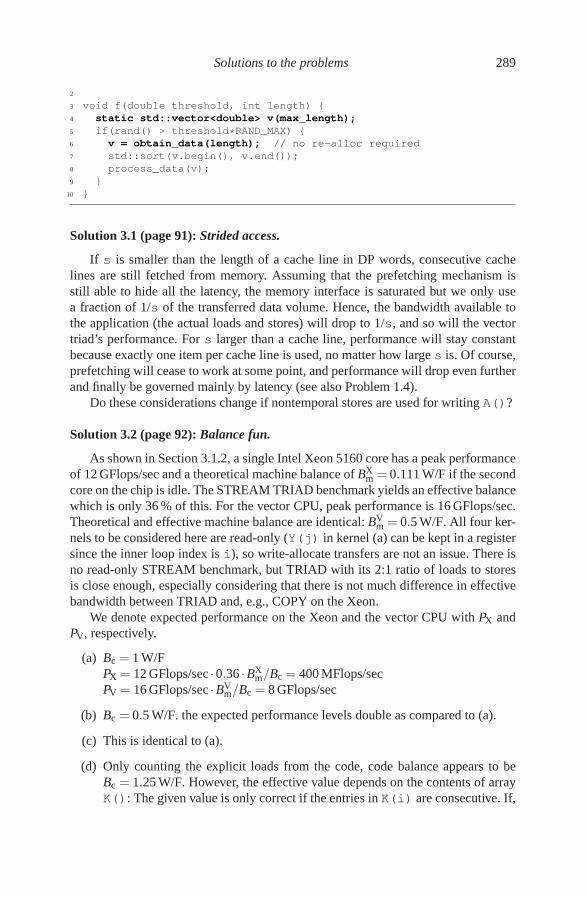
Solutions to the problems 289
2
3 void f(double threshold, int length) {
4 static std::vector<double> v(max_length);
5 if(rand() > threshold*RAND_MAX) {
6 v = obtain_data(length); // no re-alloc required
7 std::sort(v.begin(), v.end());
8 process_data(v);
9 }
10 }
Solution 3.1 (page 91): Strided access.
If s is smaller than the length of a cache line in DP words, consecutive cachelines are still fetched from memory. Assuming that the prefetching mechanism isstill able to hide all the latency, the memory interface is saturated but we only usea fraction of 1/s of the transferred data volume. Hence, the bandwidth available tothe application (the actual loads and stores) will drop to 1/s, and so will the vectortriad’s performance. For s larger than a cache line, performance will stay constantbecause exactly one item per cache line is used, no matter how large s is. Of course,prefetching will cease to work at some point, and performance will drop even furtherand finally be governed mainly by latency (see also Problem 1.4).
Do these considerations change if nontemporal stores are used for writing A()?
Solution 3.2 (page 92): Balance fun.
As shown in Section 3.1.2, a single Intel Xeon 5160 core has a peak performanceof 12 GFlops/sec and a theoretical machine balance of BX
m = 0.111 W/F if the secondcore on the chip is idle. The STREAM TRIAD benchmark yields an effective balancewhich is only 36 % of this. For the vector CPU, peak performance is 16 GFlops/sec.Theoretical and effective machine balance are identical: BV
m = 0.5 W/F. All four ker-nels to be considered here are read-only (Y(j) in kernel (a) can be kept in a registersince the inner loop index is i), so write-allocate transfers are not an issue. There isno read-only STREAM benchmark, but TRIAD with its 2:1 ratio of loads to storesis close enough, especially considering that there is not much difference in effectivebandwidth between TRIAD and, e.g., COPY on the Xeon.
We denote expected performance on the Xeon and the vector CPU with PX andPV, respectively.
(a) Bc = 1 W/FPX = 12 GFlops/sec ·0.36 ·BX
m/Bc = 400 MFlops/secPV = 16 GFlops/sec ·BV
m/Bc = 8 GFlops/sec
(b) Bc = 0.5 W/F. the expected performance levels double as compared to (a).
(c) This is identical to (a).
(d) Only counting the explicit loads from the code, code balance appears to beBc = 1.25 W/F. However, the effective value depends on the contents of arrayK(): The given value is only correct if the entries in K(i) are consecutive. If,
290 Introduction to High Performance Computing for Scientists and Engineers
e.g., K(i) = const., only one entry of B() is loaded, and Bmin,Xc = 0.75 W/F
on the cache-based CPU. A vector CPU does not have the advantage of acache, so it must re-load this value over and over again, and code balanceis unchanged. On the other hand, it can perform scattered loads efficiently,so that BV
c = 1.25 W/F independent of the contents of K() (in reality thereare deviations from this ideal because, e.g., gather operations are less efficientthan consecutive streams). Hence, the vector processor should always end upat PV = 16 GFlops/sec ·BV
m/BVc = 6.4 GFlops/sec.
The worst situation for the cache-based CPU is a completely random K(i)
with a large co-domain, so that each load from array B() incurs a full cacheline read of which only a single entry is used before eviction. With a 64-bytecache line, B
max,Xc = 4.75 W/F. Thus, the three cases are:
1. K(i)= const.:B
min,Xc = 0.75 W/F, and
PX = 12 GFlops/sec ·0.36 ·BXm/B
min,Xc = 639 MFlops/sec.
2. K(i)= i:Bc = 1.25 W/F, andPX = 12 GFlops/sec ·0.36 ·BX
m/BXc = 384 MFlops/sec.
3. K(i)= random:Bc = 4.75 W/F, andPX = 12 GFlops/sec ·0.36 ·BX
m/Bmax,Xc = 101 MFlops/sec.
This estimate is only an upper bound, since prefetching will not work.
Note that some Intel x86 processors always fetch two consecutive cache lineson each miss (can you imagine why?), further increasing code balance in theworst-case scenario.
Solution 3.3 (page 92): Performance projection.
We normalize the original runtime to T = Tm +Tc = 1, with Tm = 0.4 and Tc =0.6. The two parts of the application have different characteristics. A code balanceof 0.04 W/F means that performance is not bound by memory bandwidth but otherfactors inside the CPU core. The absolute runtime for this part will most probably becut in half if the peak performance is doubled, because the resulting machine balanceof 0.06 W/F is still larger than code balance. The other part of the application will notchange its runtime since it is clearly memory-bound at a code balance of 0.5 W/F. Insummary, overall runtime will be T = Tm +Tc/2 = 0.7.
If the SIMD vector length (and thus peak performance) is further increased, ma-chine balance will be reduced even more. At a machine balance of 0.04 W/F, theformerly CPU-bound part of the application will become memory-bound. From thatpoint, no boost in peak performance can improve its runtime any more. Overall run-time is then Tmin = Tm +Tc/3 = 0.6.
Amdahl’s Law comes to mind, and indeed above considerations are reminiscentof the concepts behind it. However, there is a slight complication because the CPU-

Solutions to the problems 291
Listing B.1: An implementation of the 3D Jacobi algorithm with three-way loop blocking.
1 double precision :: oos
2 double precision, dimension(0:imax+1,0:jmax+1,0:kmax+1,0:1) :: phi
3 integer :: t0,t1
4 t0 = 0 ; t1 = 1 ; oos = 1.d0/6.d0
5 ...
6 ! loop over sweeps
7 do s=1,ITER
8 ! loop nest over blocks
9 do ks=1,kmax,bz
10 do js=1,jmax,by
11 do is=1,imax,bx
12 ! sweep one block
13 do k=ks,min(kmax,ks+bz-1)
14 do j=js,min(jmax,js+by-1)
15 do i=is,min(imax,is+bx-1)
16 phi(i,j,k,t1) = oos * ( &
17 phi(i-1,j,k,t0)+phi(i+1,j,k,t0)+ &
18 phi(i,j-1,k,t0)+phi(i,j+1,k,t0)+ &
19 phi(i,j,k-1,t0)+phi(i,j,k+1,t0) )
20 enddo
21 enddo
22 enddo
23 enddo
24 enddo
25 enddo
26 i=t0 ; t0=t1; t1=i ! swap arrays
27 enddo
bound part of the application becomes memory-bound at some critical machine bal-ance so that the absolute performance limit is actually reached, as opposed to Am-dahl’s Law where it is an asymptotic value.
Solution 3.4 (page 92): Optimizing 3D Jacobi.
Compared to the 2D Jacobi case, we can expect more performance breakdownswhen increasing the problem size: If two successive k-planes fit into cache, only oneof the six loads generates a cache miss. If the cache is only large enough to holdtwo successive j-lines per k-plane, three loads go to memory (one for each k-planeinvolved in updating a stencil). Finally, at even larger problem sizes only a singleload can be satisfied from cache. This would only happen with ridiculously largeproblems, or if the computational domain has a very oblong shape, so it will not beobservable in practice.
As in the matrix transpose example, loop blocking eliminates those breakdowns.One sweep over the complete volume can be performed as a series of sweeps oversubvolumes of size bx×by×bz. Those can be chosen small enough so that twosuccessive k-layers fit easily into the outer-level cache. A possible implementation isshown in Listing B.1. Note that we are not paying attention to optimizations like data

292 Introduction to High Performance Computing for Scientists and Engineers
alignment or nontemporal stores here.Loop blocking in the variant shown above is also called spatial blocking. It can
eliminate all performance breakdowns after the problem is too large for the outerlevel cache, i.e., it can maintain a code balance of 0.5 W/F (3 Words per 6 Flops,including write allocates). The question remains: What is the optimal choice for theblock sizes? In principle, a block should be small enough in the i and j directions sothat at least two successive k-planes fit into the portion of the outer-level cache thatis available to a core. A “safety factor” should be included because the full cachecapacity can never be used. Note also that hardware prefetchers (especially on x86processors) and the penalties connected with TLB misses demand that the memorystreams handled in the inner loop should not be significantly shorter than one page.
In order to decrease code balance even further one has to include the iterationloop into the blocking scheme, performing more than one stencil update on everyitem loaded to the cache. This is called temporal blocking. While it is conceptu-ally straightforward, its optimal implementation, performance properties, and inter-actions with multicore structures are still a field of active research [O61, O73, O74,O75, O52, O53].
Solution 3.5 (page 93): Inner loop unrolling revisited.
Stencil codes can benefit from inner loop unrolling because onecan save loadsfrom cache to registers. For demonstration we consider a very simple “two-pointstencil”:
1 do i=1,n-1
2 b(i) = a(i) + s*a(i+1)
3 enddo
In each iteration, two loads and one store appear to be required to perform the updateon b(i). However, a(i+1) could be kept in a register and re-used immediately inthe next iteration (we are ignoring a possible loop remainder here):
1 do i=1,n-1,2
2 b(i) = a(i) + s*a(i+1)
3 b(i+1) = a(i+1) + s*a(i+2)
4 enddo
This saves half of the loads from array a(). However, it is an in-cache optimizationsince the extra load in the version without unrolling always comes from L1 cache.The unrolling will thus have no advantage for long, memory-bound loops. In simplecases, compilers will employ this variant of inner loop unrolling automatically.
It is left to the reader to figure out how inner loop unrolling may be applied to theJacobi stencil.
Solution 3.6 (page 93): Not unrollable?
In principle, unroll and jam is only possible if the loop nest is “rectangular,” i.e.,if the inner loop bounds do not depend on the outer loop index. This condition is
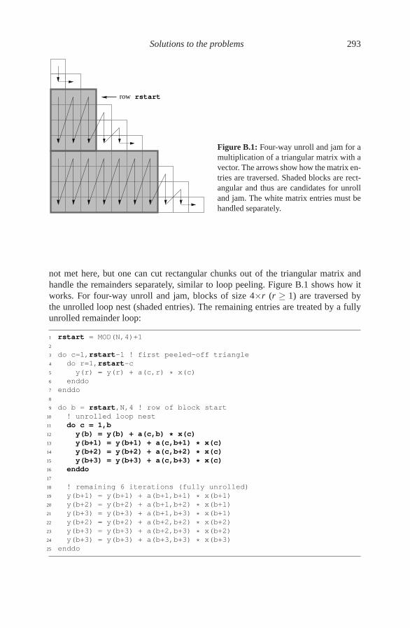
Solutions to the problems 293
row rstart
Figure B.1: Four-way unroll and jam for amultiplication of a triangular matrix with avector. The arrows show how the matrix en-tries are traversed. Shaded blocks are rect-angular and thus are candidates for unrolland jam. The white matrix entries must behandled separately.
not met here, but one can cut rectangular chunks out of the triangular matrix andhandle the remainders separately, similar to loop peeling. Figure B.1 shows how itworks. For four-way unroll and jam, blocks of size 4×r (r ≥ 1) are traversed bythe unrolled loop nest (shaded entries). The remaining entries are treated by a fullyunrolled remainder loop:
1 rstart = MOD(N,4)+1
2
3 do c=1,rstart-1 ! first peeled-off triangle
4 do r=1,rstart-c
5 y(r) = y(r) + a(c,r) * x(c)
6 enddo
7 enddo
8
9 do b = rstart,N,4 ! row of block start
10 ! unrolled loop nest
11 do c = 1,b
12 y(b) = y(b) + a(c,b) * x(c)
13 y(b+1) = y(b+1) + a(c,b+1) * x(c)
14 y(b+2) = y(b+2) + a(c,b+2) * x(c)
15 y(b+3) = y(b+3) + a(c,b+3) * x(c)
16 enddo
17
18 ! remaining 6 iterations (fully unrolled)
19 y(b+1) = y(b+1) + a(b+1,b+1) * x(b+1)
20 y(b+2) = y(b+2) + a(b+1,b+2) * x(b+1)
21 y(b+3) = y(b+3) + a(b+1,b+3) * x(b+1)
22 y(b+2) = y(b+2) + a(b+2,b+2) * x(b+2)
23 y(b+3) = y(b+3) + a(b+2,b+3) * x(b+2)
24 y(b+3) = y(b+3) + a(b+3,b+3) * x(b+3)
25 enddo

294 Introduction to High Performance Computing for Scientists and Engineers
Solution 3.7 (page 93): Application optimization.
This code has the following possible performance issues:
• The inner loop is dominated by computationally expensive (“strong”) trigono-metric functions.
• There is a rather expensive integer modulo operation (much slower than anyother integer arithmetic or logical instruction).
• Access to matrices mat and s is strided because the inner loop goes over j.SIMD vectorization will not work.
Pulling the expensive operations out of the inner loop is the first and most simplestep (this should really be done by the compiler, though). At the same time, we cansubstitute the modulo by a bit mask and the complicated trigonometric expression bya much simpler one:
1 do i=1,N
2 val = DBLE(IAND(v(i),255))
3 val = -0.5d0*COS(2.d0*val)
4 do j=1,N
5 mat(i,j) = s(i,j) * val
6 enddo
7 enddo
Although this optimization boosts performance quite a bit, the strided access in theinner loop is hazardous, especially when N gets large (see Section 3.4). We can’t justinterchange the loop levels, because that would move the expensive operations to theinside again. Instead we note that the cosine is evaluated on 256 distinct values only,so it can be tabulated:
1 double precision, dimension(0:255), save :: vtab
2 logical, save :: flag = .TRUE.
3 if(flag) then ! do this only once
4 flag = .FALSE.
5 do i=0,255
6 vtab(i) = -0.5d0*COS(2.d0*DBLE(i))
7 enddo
8 endif
9 do j=1,N
10 do i=1,N
11 mat(i,j) = s(i,j) * vtab(IAND(v(i),255))
12 enddo
13 enddo
In a memory-bound situation, i.e., for large N, this is a good solution because theadditional indirection will be cheap, and vtab() will be in the cache all the time.Moreover, the table must be computed only once. If the problem fits into the cache,however, SIMD vectorizability becomes important. One way to vectorize the innerloop is to tabulate not just the 256 trigonometric function values but the whole factorafter s(i,j):

Solutions to the problems 295
1 double precision, dimension(0:255), save :: vtab
2 double precision, dimension(N) :: ftab
3 logical, save :: flag = .TRUE.
4 if(flag) then ! do this only once
5 flag = .FALSE.
6 do i=0,255
7 vtab(i) = -0.5d0*COS(2.d0*DBLE(i))
8 enddo
9 endif
10 do i=1,N ! do this on every call
11 ftab(i) = vtab(IAND(v(i),255))
12 enddo
13 do j=1,N
14 do i=1,N
15 mat(i,j) = s(i,j) * ftab(i)
16 enddo
17 enddo
Since v() may change between calls of the function, ftab() must be recomputedevery time, but the inner loop is now trivially SIMD-vectorizable.
Solution 3.8 (page 93): TLB impact.
TLB “cache lines” are memory pages, so the penalty for a miss must be comparedto the time it takes to stream one page into cache. At present, memory bandwidthis a few GBytes/sec per core, leading to a transfer time of around 1 µs for a 4 kBpage. The penalty for a TLB miss varies widely across architectures, but it is usuallyfar smaller than 100 CPU cycles. At clock frequencies of around 2 GHz, one TLBmiss per page on a pure streaming code has no noticeable impact on performance. Ifsignificantly less than a page is transferred before going to the next, this will change,of course.
Some systems have larger memory pages, or can be configured to use them. Atbest, the complete working set of an application can be mapped by the TLB, so thatthe number of misses is zero. Even if this is not the case, large pages can enhance theprobability of TLB hits, because it becomes less likely that a new page is hit at anygiven moment. However, switching to large pages also usually reduces the numberof available TLB entries.
Solution 4.1 (page 114): Building fat-tree network hierarchies.
Static routing assigns a fixed network route to each pair of communication part-ners. With a 2:3 oversubscription, some connections will get less bandwidth into thespine because it is not possible to distribute the leaves evenly among the spine con-nections (the number of leaves on a leaf switch is not a multiple of the number of itsconnections into the spine). Hence, the network gets even more unbalanced, beyondthe contention effects incurred by static routing and oversubscription alone.

296 Introduction to High Performance Computing for Scientists and Engineers
Solution 5.1 (page 140): Overlapping communication and computation.
Hiding communication behind computation is something that sounds straightfor-ward but is usually not easy to achieve in practice; see Sections 10.4.3 and 11.1.3 fordetails. Anyway, assuming that it is possible, the time for parallel execution in thedenominator of the strong scaling speedup function (5.30) becomes
max[
(1− s)/N,(
κN−β +λ)
µ−1]
. (B.1)
This describes a crossover from perfectly to partially hidden communication when
µ(1− s) = κN1−βc +λNc . (B.2)
As the right-hand side of this equation is strictly monotonous in Nc if 0 ≤ β ≤ 1,the crossover will always be shifted to larger N on the slow computer (µ > 1). Byhow much exactly (a factor of at least µ is certainly desirable) is given by the ratioNc(µ)/Nc(µ = 1), but solving for Nc is not easily possible. Fortunately, it is sufficientto investigate the important limits λ = 0 and κ = 0. For vanishing latency,
Nc(λ = 0) =
(
µ(1− s)
κ
)1/(1−β )
, (B.3)
andNc(µ > 1)
Nc(µ = 1)
∣
∣
∣
∣
λ=0= µ1/(1−β ) > µ . (B.4)
In the latency-dominated limit κ = 0 we immediately get
Nc(µ > 1)
Nc(µ = 1)
∣
∣
∣
∣
κ=0= µ . (B.5)
We have derived an additional benefit of slow computers: If communication can behidden behind computation, it becomes noticeable at a certain N, which is at least µtimes larger than on the standard computer.
Can you do the same analysis for weak scaling?
Solution 5.2 (page 141): Choosing an optimal number of workers.
For strong scaling and latency-dominated communication, the walltime for exe-cution (“time to solution”) is
Tw = s+1− s
N+λ (B.6)
if s is the nonparallelizable fraction and λ is the latency. The cost for using N pro-cessors for a time Tw is NTw, yielding a cost-walltime product of
V = NT 2w = N
(
s+1− s
N+λ
)2
, (B.7)

Solutions to the problems 297
which is extremal if
∂V
∂N=
1N2 [(1+λN +(N −1)s)(s−1+N(λ + s))] = 0 . (B.8)
The only positive solution of this equation in N is
Nopt =1− s
λ + s. (B.9)
Interestingly, if we assume two-dimensional domain decomposition with halo ex-change so that
Tw = s+1− s
N+λ +κN−1/2 , (B.10)
the result is the same as in (B.9), i.e., independent of κ . This is a special case, how-ever; any other power of N in the communication overhead leads to substantiallydifferent results (and a much more complex derivation).
Finally, the speedup obtained at N = Nopt is
Sopt =
(
2(s+λ )+κ
√
λ + s
1− s
)−1
. (B.11)
A comparison with the maximum speedup Smax = 1/(λ + s) yields
Smax
Sopt= 2+
κ√
(1− s)(λ + s), (B.12)
so for κ = 0 the “sweet spot” lies at half the maximum speedup, and even lower forfinite κ .
Of course, no matter what the parallel application’s communication requirementsare, if the workload is such that the time for a single serial application run is “toler-able,” and many such runs must be conducted, the most efficient way to use a par-allel computer is throughput mode. In throughput mode, many instances of a serialcode are run concurrently under control of a resource management system (whichis present on all production machines). This provides the best utilization of all re-sources. For obvious reasons, such a workload is not suitable for massively parallelmachines with expensive interconnect networks.
Solution 5.3 (page 141): The impact of synchronization.
Synchronization appears at the same place as communication overhead, leadingto eventual slowdown with strong scaling. For weak scaling, linear scalability is de-stroyed; linear sync overhead even leads to saturation.
Solution 5.4 (page 141): Accelerator devices.
Ignoring communication aspects (e.g., overhead for moving data into and out ofthe accelerator), we can model the situation by assuming that the accelerated parts

298 Introduction to High Performance Computing for Scientists and Engineers
of the application execute α times faster than on the host, whereas the rest staysunchanged. Using Amdahl’s Law, s is the host part and p = 1− s is the acceleratedpart. Therefore, the asymptotic performance is governed by the host part; if, e.g., α =100 and s = 10−2, the speedup is only 50, and we are wasting half of the accelerator’scapability. To get a speedup of rα with 0 < r < 1, we need to solve
1
s+ 1−sα
= rα (B.13)
for s, leading to
s =r−1 −1α −1
, (B.14)
which yields s ≈ 1.1× 10⁻³ at r = 0.9 and α = 100. The lesson is that efficientuse of accelerators requires a major part of original execution time (much more thanjust 1− 1/α) to be moved to special hardware. Incidentally, Amdahl had formu-lated his famous law in his original paper along the lines of “accelerated execu-tion” versus “housekeeping and data management” effort on the ILLIAC IV super-computer [R40], which implemented a massively data-parallel SIMD programmingmodel:
A fairly obvious conclusion which can be drawn at this point is that the effortexpended on achieving high parallel processing rates is wasted unless it is ac-companied by achievements in sequential processing rates of very nearly thesame magnitude. [M45]
This statement fits perfectly to the situation described above. In essence, it was al-ready derived mathematically in Section 5.3.5, albeit in a slightly different context.
One may argue that enlarging the (accelerated) problem size would mitigate theproblem, but this is debatable because of the memory size restrictions on acceleratorhardware. The larger the performance of a computational unit (core, socket, node,accelerator), the larger its memory must be to keep the serial (or unaccelerated) partand communication overhead under control.
Solution 6.1 (page 162): OpenMP correctness.
The variable noise in subroutine f() carries an implicit SAVE attribute, be-cause it is initialized on declaration. Its initial value will thus only be set on the firstcall, which is exactly what would be intended if the code were serial. However, call-ing f() from a parallel region makes noise a shared variable, and there will bea race condition. To correct this problem, either noise should be provided as anargument to f() (similar to the seed in thread safe random number generators), orits update should be protected via a synchronization construct.
Solution 6.2 (page 162): π by Monte Carlo.
The key ingredient is a thread safe random number generator. According to theOpenMP standard [P11], the RANDOM_NUMBER() intrinsic subroutine in Fortran 90

Solutions to the problems 299
is supposed to be thread safe, so it could be used here. However, there are perfor-mance implications (why?), and it is usually better to avoid built-in generators any-way (see, e.g., [N51] for a thorough discussion), so we just assume that there is afunction ran_gen(), which essentially behaves like the rand_r() function fromPOSIX: It takes a reference to an integer random seed, which is updated on each calland stored in the calling function, separately for each thread. The function returns aninteger between 0 and 231, which is easily converted to a floating-point number inthe required range:
1 integer(kind=8) :: sum
2 integer, parameter :: ITER = 1000000000
3 integer :: seed, i
4 double precision, parameter :: rcp = 1.d0/2**31
5 double precision :: x,y,pi
6 !$OMP PARALLEL PRIVATE(x,y,seed) REDUCTION(+:sum)
7 seed = omp_get_thread_num() ! everyone gets their own seed
8 !$OMP DO
9 do i=1,ITER
10 x = ran_gen(seed)*rcp
11 y = ran_gen(seed)*rcp
12 if (x*x + y*y .le. 1.d0) sum=sum+1
13 enddo
14 !$OMP END DO
15 !$OMP END PARALLEL
16 pi = (4.d0 * sum) / ITER
In line 7, the threads’ private seeds are set to distinct values. The “hit count” for thequarter circle in the first quadrant is obtained from a reduction operation (summationacross all threads) in sum, and used in line 16 to compute the final result for π .
Using different seeds for all threads is vital because if each thread produces thesame sequence of pseudorandom numbers, the statistical error would be the same asif only a single thread were running.
Solution 6.3 (page 163): Disentangling critical regions.
Evaluation of func() does not have to be protected by a critical region at all (asopposed to the update of sum). It can be done outside, and the two critical regionswill not interfere any more:
1 !$OMP PARALLEL DO PRIVATE(x)
2 do i=1,N
3 x = SIN(2*PI*DBLE(i)/N)
4 x = func(x)
5 !$OMP CRITICAL
6 sum = sum + x
7 !$OMP END CRITICAL
8 enddo
9 !$OMP END PARALLEL DO
10 ...
11 double precision FUNCTION func(v)
12 double precision :: v
13 !$OMP CRITICAL

300 Introduction to High Performance Computing for Scientists and Engineers
14 func = v + random_func()
15 !$OMP END CRITICAL
16 END SUBROUTINE func
Solution 6.4 (page 163): Synchronization perils.
A barrier must always be encountered by all threads in the team. This is notguaranteed in a workshared loop.
Solution 6.5 (page 163): Unparallelizable?
Thanks to Jakub Jelinek from Red Hat for providing this solution. Clearly, theloop can be parallelized right away if we realize that opt(n)=up**n, but expo-nentiation is so expensive that we’d rather not take this route (although scalabilitywill be great if we take the single-thread performance of the parallel code as a base-line [S7]). Instead we revert to the original (fast) version for calculating opt(n) ifwe are sure that the previous iteration handled by this thread was at n-1 (line 12).On the other hand, if we are at the start of a new chunk, indices were skipped andopt(n) must be calculated by exponentiation (line 14):
1 double precision, parameter :: up = 1.00001d0
2 double precision :: Sn, origSn
3 double precision, dimension(0:len) :: opt
4 integer :: n, lastn
5
6 origSn = 1.d0
7 lastn = -2
8
9 !$OMP PARALLEL DO FIRSTPRIVATE(lastn) LASTPRIVATE(Sn)
10 do n = 0,len
11 if(lastn .eq. n-1) then ! still in same chunk?
12 Sn = Sn * up ! yes: fast version
13 else
14 Sn = origSn * up**n ! no: slow version
15 endif
16 opt(n) = Sn
17 lastn = n ! storing index
18 enddo
19 !$OMP END PARALLEL DO
20 Sn = Sn * up
The LASTPRIVATE(Sn) clause ensures that Sn has the same value as in the serialcase after the loop is finished. FIRSTPRIVATE(lastn) assigns the initial value oflastn to its private copies when the parallel region starts. This is purely for conve-nience, because we could have done the copying manually by splitting the combinedPARALLEL DO directive.
While the solution works for all OpenMP loop scheduling options, it will beespecially slow for static or dynamic scheduling with small chunksizes. In the specialcase of “STATIC,1” it will be just as slow as using exponentiation from the start.

Solutions to the problems 301
Solution 6.6 (page 163): Gauss–Seidel pipelined.
This optimization is also called loop skewing. Starting with a particular site, allsites that can be updated at the same time are part of a so-called hyperplane and fulfillthe condition i+ j+k = const. = 3n, with n ≥ 1. Pipelined execution is now possibleas all inner loop iterations are independent, enabling efficient use of vector pipes(see Section 1.6). Cache-based processors, however, suffer from the erratic accesspatterns generated by the hyperplane method. Cache lines once fetched for a certainstencil update do not stay in cache long enough to exploit spatial locality. Bandwidthutilization (as seen from the application) is thus very poor. This is why the standardformulation of the Gauss–Seidel loop nest together with wavefront parallelizationis preferable for cache-based microprocessors, despite the performance loss frominsufficient pipelining.
Solution 7.1 (page 184): Privatization gymnastics.
In C/C++, reduction clauses cannot be applied to arrays. The reduction mustthus be done manually. A firstprivate clause helps with initializing the privatecopies of s[]; in a “true” OpenMP reduction, this would be automatic as well:
1 int s[8] = {0};
2 int *ps = s;
3
4 #pragma omp parallel firstprivate(s)
5 {
6 #pragma omp for
7 for(int i=0; i<N; ++i)
8 s[a[i]]++;
9 #ifdef _OPENMP
10 #pragma omp critical
11 {
12 for(int i=0; i<8; ++i) { // reduction loop
13 ps[i] += s[i];
14 }
15 } // end critical
16 #endif
17 } // end parallel
Using conditional compilation, we skip the explicit reduction if the code is compiledwithout OpenMP.
Similar measures must be taken even in Fortran if the reduction operator to beused is not supported directly by OpenMP. Likewise, overloaded C++ operators arenot allowed in reduction clauses even on scalar types.
Solution 7.2 (page 184): Superlinear speedup.
Figure B.2 shows that the described situation occurs at a problem size around6002: A single 4 MB L2 cache is too small to accommodate the working set, but8 MB is sufficient. The speedup when going from one (or two) threads to four is 5.4.
When the working set fits into cache, the grid updates are so fast that typical

302 Introduction to High Performance Computing for Scientists and Engineers
100 1000N
0
500
1000
1500
Perf
orm
ance [M
LU
Ps/s
ec] 1 thread
2 threads1 socket
4 threads
8 MB L2
4 MB L2
5.4x speedup
so
cke
t
32k L1D 32k L1D 32k L1D 32k L1D
Chipset
Memory
P P P P
4MB L2 4MB L2
Figure B.2: Superlinear speedup with the 2D Jacobi solver (same data as in Figure 6.3). Ata problem size of 6002, the working set is too large to fit into one socket’s L2 cache, soperformance is close to memory-bound (filled symbols). Using two additional threads (opendiamonds), 8 MB cache become available, which is large enough to accommodate all data.Hence, the 5.4× speedup.
OpenMP overhead, especially implicit barriers (see Section 7.2.2), might dominateruntime if the number of threads is large. To find a criterion for this we must com-pare the time for one sweep with a typical synchronization overhead. Looking atthe maximum two-thread in-cache performance (filled squares), we estimate that asingle sweep takes about 170 µs. As a very rough guideline we may assume that syn-chronizing all threads in a shared-memory machine requires about 1 µs per socket ifthe barrier is implemented efficiently [M41]. Hence, on standard two- or four-socketnodes one should be able to observe superlinear scaling for this kind of problem.
Solution 7.3 (page 184): Reductions and initial values.
If the code is compiled without OpenMP support, it should still produce correctresults, which it doesn’t if R is not initialized. If we could use C(j) as a reductionvariable, this detour would not be necessary, but only named variables are allowed inreduction clauses.
Solution 7.4 (page 184): Optimal thread count.
Parallelism adds overhead, so one should use as few threads as possible. Theoptimal number is given by the scalability of main memory bandwidth versus threadcount. If two out of six threads already saturate a socket’s memory bus, running morethan four threads does not make sense. All the details about cache groups and systemarchitecture are much less relevant.
Note that shared caches often do not provide perfect bandwidth scaling as well,so this reasoning may apply to in-cache computations, too [M41].

Solutions to the problems 303
Solution 8.1 (page 201): Dynamic scheduling and ccNUMA.
As usual, performance (P) is work (W ) divided by time (t). We choose W = 2,meaning that two memory pages are to be assigned to the two running threads. Eachchunk takes a duration of t = 1 to execute locally, so that P = 2p if there is nononlocal access. In general, four cases must be distinguished:
1. Both threads access their page locally: t = 1.
2. Both threads have to access their page remotely: Since the inter-LD network isassumed to be infinitely fast, and there is no contention on either memory bus,we have t = 1.
3. Both threads access their page in LD0: Contention on this memory bus leadsto t = 2.
4. Both threads access their page in LD1: Contention on this memory bus leadsto t = 2.
These four cases occur with equal probability, so the average time to stream the twopages is tavg = (1 + 1 + 2 + 2)/4 = 1.5. Hence, P = W/tavg = 4p/3, i.e., the coderuns 33% slower than with perfect access locality.
This derivation is so simple because we deal with only two locality domains, andthe elementary work package is two pages no matter where they are mapped. Canyou generalize the analysis to an arbitrary number of locality domains?
Solution 8.2 (page 202): Unfortunate chunksizes.
There are two possible reasons for bad performance at small chunksizes:
• This is a situation in which the hardware-based prefetching mechanisms ofx86-based processors are actually counterproductive. Once activated by a num-ber of successive cache misses (two in this case), the prefetcher starts transfer-ring data to cache until the end of the current page is reached (or until can-celed). If the chunksize is smaller than a page, some of this data is not neededand will only waste bandwidth and cache capacity. The closer the chunksizegets to the page size, the smaller this effect.
• A small chunksize will also increase the number of TLB misses. The actualperformance impact of TLB misses is strongly processor-dependent. See alsoProblem 3.8.
Solution 8.3 (page 202): Speeding up “small” jobs.
If multiple streams are required, round-robin placement may yield better single-socket performance than first touch because part of the bandwidth can be satisfiedvia remote accesses. The possible benefit of this strategy depends strongly on thehardware, though.
304 Introduction to High Performance Computing for Scientists and Engineers
Solution 8.4 (page 202): Triangular matrix-vector multiplication.
Parallelizing the inner reduction loop would be fine, but will only work with verylarge problems because of OpenMP overhead and NUMA placement problems. Theouter loop, however, has different workloads for different iterations, so there is asevere load balancing problem:
1 !$OMP PARALLEL DO SCHEDULE(RUNTIME)
2 do r=1,N ! parallel initialization
3 y(r) = 0.d0
4 x(r) = 0.d0
5 do c=1,r
6 a(c,r) =0.d0
7 enddo
8 enddo
9 !$OMP END PARALLEL DO
10 ...
11 !$OMP PARALLEL DO SCHEDULE(RUNTIME)
12 do r=1,N ! actual triangular MVM loop
13 do c=1,r
14 y(r) = y(r) + a(c,r) * x(c)
15 enddo
16 enddo
17 !$OMP END PARALLEL DO
We have added the parallel initialization loop for good page placement in ccNUMAsystems.
Standard static scheduling is certainly not a good choice here. Guided or dynamicscheduling with an appropriate chunksize could balance the load without too muchoverhead, but leads to nonlocal accesses on ccNUMA because chunks are assigneddynamically at runtime. Hence, the only reasonable alternative is static scheduling,and a chunksize that enables proper NUMA placement at least for matrix rows thatare not too close to the “tip” of the triangle.
What about the placement issues for x()?
Solution 8.5 (page 202): NUMA placement by overloading.
The parallel loop schedule is the crucial point. The loop schedules of the ini-tialization and worksharing loops should be identical. Had we used a single loop, apossible chunksize would be interpreted as a multiple of one loop iteration, whichtouches a single char. A chunksize on a worksharing loop handling objects of typeD would refer to units of sizeof(D), and NUMA placement would be wrong.
Solution 9.1 (page 233): Shifts and deadlocks.
Exchanging the order of sends and receives also works with an odd number ofprocesses. The “leftover” process will just have to wait until its direct neighbors havefinished communicating. See Section 10.3.1 for a discussion of the “open chain”case.

Solutions to the problems 305
Solution 9.2 (page 233): Deadlocks and nonblocking MPI.
Quoting the MPI standard (Section 3.7):
In all cases, the send start call [meaning a nonblocking send; note from theauthors] is local: it returns immediately, irrespective of the status of other pro-cesses. If the call causes some system resource to be exhausted, then it will failand return an error code. Quality implementations of MPI should ensure that thishappens only in “pathological” cases. That is, an MPI implementation should beable to support a large number of pending nonblocking operations. [P15]
This means that using nonblocking calls is a reliable way to prevent deadlocks, be-cause the MPI standard does not allow a pair of matching send and receives on twoprocesses to remain permanently outstanding.
Solution 9.3 (page 234): Open boundary conditions.
For open boundary conditions there would be no plateaus up to 12 processes,because the maximum number of faces to communicate per subdomain changes withevery new decomposition. However, we would see a plateau between 12 and 16 pro-cesses: There is no new subdomain type (in terms of communication characteristics)when going from (3,2,2) to (4,2,2). If there are at least three subdomains in each di-rection, there are no fundamental changes any more and the ratio between ideal andreal performance is constant. This is the case at a minimum of 27 processes (3,3,3).
Solution 9.4 (page 234): A performance model for strong scaling of the parallel
Jacobi code.
The smallest subdomain size (at 3× 2× 2 = 12 processors) is 40× 602, takingroughly 1 ms for a single sweep. The 50 µs latency is multiplied by k = 6 in thiscase, so the aggregated latency is already nearly one third of Ts. One may expectthat the overhead for MPI_Reduce() is a small multiple of the PingPong latencyif implemented efficiently (measured value is between 50 µs and 230 µs on 1–12nodes, and this of course depends on N as well). With these refinements, the modelis able to reproduce the strong scaling data quite well.
Solution 9.5 (page 234): MPI correctness.
The receive on process 1 matches the send on process 0, but the latter may neverget around to calling MPI_Send(). This is because collective communication rou-tines may, but do not have to, synchronize all processes in the communicator (ofcourse, MPI_Barrier() synchronizes by definition). If the broadcast is synchro-nizing, we have a classic deadlock since the receive on process 1 waits forever for itsmatching send.

306 Introduction to High Performance Computing for Scientists and Engineers
t1 t2 t3 t4 t5 t6
Rank
0
1
2
3
4
5
6
7
Time step
(a) (b)t1 t2 t3
Time step
0
1
2
3
4
5
6
7
Rank
Figure B.3: “Emulating” MPI_Allreduce() by a reduction followed by a broadcast (a)serializes the two operations and leaves a lot of network resources idling. An optimized“butterfly”-style pattern (b) saves a lot of time if the network is nonblocking.
Solution 10.1 (page 260): Reductions and contention.
The number of transmitted messages is the same in both cases. So if any twotransfers cannot overlap, linear and logarithmic reduction have the same perfor-mance. A bus network (see Section 4.5.2) has this property.
Even on a fully nonblocking switched network, contention can occur if staticrouting is used (see Section 4.5.3).
Solution 10.2 (page 260): Allreduce, optimized.
Doing a reduction followed by a broadcast takes the sum of their runtimes (seeFigure B.3(a)). Instead, an optimized MPI_Allreduce() operation can save a lotof time by utilizing the available parallelism in the network (see Figure B.3(b)).
Solution 10.3 (page 260): Eager vs. rendezvous.
In a typical “master-worker” pattern (see Section 5.2.2) workers may flood themaster with eager messages if the message size is below the eager limit. Most MPIimplementations can be configured to reserve larger buffers for storing eager mes-sages. Using MPI_Issend() could also be an alternative.
Solution 10.4 (page 260): Is cubic always optimal?
Mathematically (see Figure 10.9), “pole” decomposition is better than cubic sub-domains for N < 11. The only whole number below 11 with at least three primefactors is 8. If we decompose a cube into 2× 2× 2 versus 2× 4 subdomains and
Solutions to the problems 307
assume periodic boundary conditions, the latter variant has indeed a smaller domaincut surface. However, the difference vanishes for open boundaries.
Note that we have cheated a little here: The formulae in Figure 10.9 assumethat subdomains are always cubic, and that poles always have a square base. This isnot the case for N = 8. But you may have figured out by now that this is all just areally academic exercise; the rule that 3D decompositions incur less communicationoverhead does hold in practice.
Solution 10.5 (page 260): Riding the PingPong curve.
Beff(N,L,w,Tℓ,B) =
[
TℓN2/3
wL2 +B−1
]−1
(B.15)
As N increases, so does the influence of latency over bandwidth. This effect is partlycompensated by a large site data size w and a large linear problem size L. The latterdependency is just another example for the general rule that larger problems lead tobetter scalability (in this case because of reduced communication overhead).
Note that one should always make sure that parallel efficiency is still acceptableif communication plays any role. The “ping-pong ride” may well be meaningless ifthe application spends a significant fraction of its time communicating. One wouldthen not even consider increasing N even further, except for getting more memory.
Solution 10.6 (page 261): Nonblocking Jacobi revisited.
Each outstanding request requires a separate message buffer, so we need twelveintermediate buffers if all halo communications are to be handled with nonblock-ing MPI. Since this is a surface-versus-volume effect, the additional memory re-quirements are usually negligible. Furthermore, MPI_Wait() must be replaced byMPI_Waitany() or MPI_Waitsome().
Solution 10.7 (page 261): Send and receive combined.
1 call MPI_Isend(...)
2 call MPI_Irecv(...)
3 call MPI_Waitall(...)
A possible useful side effect is that the MPI library may perform full-duplex transfersif a send and a receive operation are outstanding at the same time. Current MPIimplementations do this.
Solution 10.8 (page 261): Load balancing and domain decomposition.
If all subdomains are of equal size, inner subdomains are laggers. Although theircomputational load is no different from all others, they must spend more time com-municating, which leads to load imbalance. However, those inner domains dominate(by number) if the number of processes is large. Boundary subdomains are speeders,

308 Introduction to High Performance Computing for Scientists and Engineers
and few speeders are tolerable (see Section 5.3.9), so this is not a problem on thelarge scale. On the other hand, if there are only like 3× 3× 3 = 27 processes, onemay think about enlarging the boundary subdomains to get better load balancing if
communication overhead is a problem at all.

Bibliography
Standard works
[S1] S. Goedecker and A. Hoisie. Performance Optimization of Numerically
Intensive Codes (SIAM), 2001. ISBN 978-0898714845.
[S2] R. Gerber, A. J. C. Bik, K. Smith and X. Tian. The Software Optimization
Cookbook (Intel Press), 2nd ed., 2005. ISBN 978-0976483212.
[S3] K. Dowd and C. Severance. High Performance Computing (O’Reilly &Associates, Inc., Sebastopol, CA, USA), 1998. ISBN 156592312X.
[S4] K. R. Wadleigh and I. L. Crawford. Software Optimization for High-Per-
formance Computing (Prentice Hall), 2000. ISBN 978-0130170088.
[S5] W. Schönauer. Scientific Supercomputing: Architecture and Use of Shared
and Distributed Memory Parallel Computers (Self-edition), 2000.http://www.rz.uni-karlsruhe.de/~rx03/book
[S6] T. G. Mattson, B. A. Sanders and B. L. Massingill. Patterns for Parallel
Programming (Addison-Wesley), 2004. ISBN 978-0-321-22811-6.
[S7] D. H. Bailey. Highly parallel perspective: Twelve ways to fool the masses
when giving performance results on parallel computers. SupercomputingReview 4(8), (1991) 54–55. ISSN 1048-6836.http://crd.lbl.gov/~dhbailey/dhbpapers/twelve-ways.pdf
Parallel programming
[P8] S. Akhter and J. Roberts. Multi-Core Programming: Increasing Per-
formance through Software Multithreading (Intel Press), 2006. ISBN0-9764832-4-6.
[P9] D. R. Butenhof. Programming with POSIX Threads (Addison-Wesley),1997. ISBN 978-0201633924.
[P10] J. Reinders. Intel Threading Building Blocks: Outfitting C++ for Multi-Core
Processor Parallelism (O’Reilly), 2007. ISBN 978-0596514808.
[P11] The OpenMP API specification for parallel programming.http://openmp.org/wp/openmp-specifications/
309

310 Bibliography
[P12] B. Chapman, G. Jost and R. van der Pas. Using OpenMP (MIT Press), 2007.ISBN 978-0262533027.
[P13] W. Gropp, E. Lusk and A. Skjellum. Using MPI (MIT Press), 2nd ed., 1999.ISBN 0-262-57132-3.
[P14] W. Gropp, E. Lusk and R. Thakur. Using MPI-2 (MIT Press), 1999. ISBN0-262-57133-1.
[P15] MPI: A Message-Passing Interface Standard. Version 2.2, September 2009.http://www.mpi-forum.org/docs/mpi-2.2/mpi22-report.pdf
[P16] A. Geist, A. Beguelin, J. Dongarra, W. Jiang, R. Manchek and V. Sunderam.PVM: Parallel Virtual Machine (MIT Press), 1994. ISBN 0-262-57108-0.http://www.netlib.org/pvm3/book/pvm-book.html
[P17] R. W. Numrich and J. Reid. Co-Array Fortran for Parallel Programming.SIGPLAN Fortran Forum 17(2), (1998) 1–31. ISSN 1061-7264.
[P18] W. W. Carlson, J. M. Draper, D. E. Culler, K. Yelick, E. Brooks and K. War-ren. Introduction to UPC and language specification. Tech. rep., IDA Cen-ter for Computing Sciences, Bowie, MD, 1999.http://www.gwu.edu/~upc/publications/upctr.pdf
Tools
[T19] OProfile — A system profiler for Linux.http://oprofile.sourceforge.net/news/
[T20] J. Treibig, G. Hager and G. Wellein. LIKWID: A lightweight performance-
oriented tool suite for x86 multicore environments. Submitted.http://arxiv.org/abs/1004.4431
[T21] Intel VTune Performance Analyzer.http://software.intel.com/en-us/intel-vtune
[T22] PAPI: Performance Application Programming Interface.http://icl.cs.utk.edu/papi/
[T23] Intel Thread Profiler.http://www.intel.com/cd/software/products/asmo-na/eng/286749.htm
[T24] D. Skinner. Performance monitoring of parallel scientific applications,2005.http://www.osti.gov/bridge/servlets/purl/881368-dOvpFA/881368.pdf
[T25] O. Zaki, E. Lusk, W. Gropp and D. Swider. Toward scalable performance
visualization with Jumpshot. International Journal of High PerformanceComputing Applications 13(3), (1999) 277–288.
Bibliography 311
[T26] Intel Trace Analyzer and Collector.http://software.intel.com/en-us/intel-trace-analyzer/
[T27] VAMPIR - Performance optimization for MPI.http://www.vampir.eu
[T28] M. Geimer, F. Wolf, B. J. Wylie, E. Ábrahám, D. Becker and B. Mohr. The
SCALASCA performance toolset architecture. In: Proc. of the International
Workshop on Scalable Tools for High-End Computing (STHEC 2008) (Kos,Greece), 51–65.
[T29] M. Gerndt, K. Fürlinger and E. Kereku. Periscope: Advanced techniques
for performance analysis. In: G. R. Joubert et al. (eds.), Parallel Comput-
ing: Current and Future Issues of High-End Computing (Proceedings of
the International Conference ParCo 2005), vol. 33 of NIC Series. ISBN3-00-017352-8.
[T30] T. Klug, M. Ott, J. Weidendorfer, and C. Trinitis. autopin - Automated
optimization of thread-to-core pinning on multicore systems. Transactionson High-Performance Embedded Architectures and Compilers 3(4), (2008)1–18.
[T31] M. Meier. Pinning OpenMP threads by overloading pthread_create().http://www.mulder.franken.de/workstuff/pthread-overload.c
[T32] Portable Linux processor affinity.http://www.open-mpi.org/software/plpa/
[T33] Portable hardware locality (hwloc).http://www.open-mpi.org/projects/hwloc/
Computer architecture and design
[R34] J. L. Hennessy and D. A. Patterson. Computer Architecture: A Quantitative
Approach (Morgan Kaufmann), 4th ed., 2006. ISBN 978-0123704900.
[R35] G. E. Moore. Cramming more components onto integrated circuits. Elec-tronics 38(8), (1965) 114–117.
[R36] W. D. Hillis. The Connection Machine (MIT Press), 1989. ISBN 978-0262580977.
[R37] N. R. Mahapatra and B. Venkatrao. The Processor-Memory Bottleneck:
Problems and Solutions. Crossroads 5, (1999) 2. ISSN 1528-4972.
[R38] M. J. Flynn. Some computer organizations and their effectiveness. IEEETrans. Comput. C-21, (1972) 948.
[R39] R. Kumar, D. M. Tullsen, N. P. Jouppi and P. Ranganathan. Heterogeneous
chip multiprocessors. IEEE Computer 38(11), (2005) 32–38.

312 Bibliography
[R40] D. P. Siewiorek, C. G. Bell and A. Newell (eds.). Computer Structures:
Principles and Examples (McGraw-Hill), 2nd ed., 1982. ISBN 978-0070573024.http://research.microsoft.com/en-us/um/people/gbell/Computer_
Structures_Principles_and_Examples/
Performance modeling
[M41] J. Treibig, G. Hager and G. Wellein. Multi-core architectures: Complexities
of performance prediction and the impact of cache topology. In: S. Wag-ner et al. (eds.), High Performance Computing in Science and Engineering,
Garching/Munich 2009 (Springer-Verlag, Berlin, Heidelberg). To appear.http://arxiv.org/abs/0910.4865
[M42] S. Williams, A. Waterman and D. Patterson. Roofline: An insightful vi-
sual performance model for multicore architectures. Commun. ACM 52(4),(2009) 65–76. ISSN 0001-0782.
[M43] P. F. Spinnato, G. van Albada and P. M. Sloot. Performance modeling of dis-
tributed hybrid architectures. IEEE Trans. Parallel Distrib. Systems 15(1),(2004) 81–92.
[M44] J. Treibig and G. Hager. Introducing a performance model for bandwidth-
limited loop kernels. In: Proceedings of PPAM 2009, the Eighth Interna-
tional Conference on Parallel Processing and Applied Mathematics, Wro-
claw, Poland, September 13–16, 2009. To appear.http://arxiv.org/abs/0905.0792
[M45] G. M. Amdahl. Validity of the single processor approach to achieving large
scale computing capabilities. In: AFIPS ’67 (Spring): Proceedings of the
April 18-20, 1967, Spring Joint Computer Conference (ACM, New York,NY, USA), 483–485.
[M46] J. L. Gustafson. Reevaluating Amdahl’s law. Commun. ACM 31(5), (1988)532–533. ISSN 0001-0782.
[M47] M. D. Hill and M. R. Marty. Amdahl’s Law in the multicore era. IEEEComputer 41(7), (2008) 33–38.
[M48] X.-H. Sun and Y. Chen. Reevaluating Amdahl’s Law in the multicore era.Journal of Parallel and Distributed Computing 70(2), (2010) 183–188. ISSN0743-7315.

Bibliography 313
Numerical techniques and libraries
[N49] R. Barrett, M. Berry, T. Chan, J. Demmel, J. Donato, J. Dongarra, V. Ei-jkhout, R. Pozo, C. Romine and H. van der Vorst. Templates for the So-
lution of Linear Systems: Building Blocks for Iterative Methods (SIAM),1993. ISBN 978-0-898713-28-2.
[N50] C. L. Lawson, R. J. Hanson, D. R. Kincaid and F. T. Krogh. Basic Linear Al-
gebra Subprograms for Fortran usage. ACM Transactions on MathematicalSoftware 5(3), (1979) 308–323. ISSN 0098-3500.
[N51] W. H. Press, B. P. Flannery, S. A. Teukolsky and W. T. Vetterling. Numerical
Recipes in FORTRAN 77: The Art of Scientific Computing (v. 1) (CambridgeUniversity Press), 2nd ed., September 1992. ISBN 052143064X.http://www.nr.com/
Optimization techniques
[O52] G. Wellein, G. Hager, T. Zeiser, M. Wittmann and H. Fehske. Efficient
temporal blocking for stencil computations by multicore-aware wavefront
parallelization. Annual International Computer Software and ApplicationsConference (COMPSAC09) 1, (2009) 579–586. ISSN 0730-3157.
[O53] M. Wittmann, G. Hager and G. Wellein. Multicore-aware parallel temporal
blocking of stencil codes for shared and distributed memory. In: Workshop
on Large-Scale Parallel Processing 2010 (IPDPS2010), Atlanta, GA, April
23, 2010.http://arxiv.org/abs/0912.4506
[O54] G. Hager, T. Zeiser, J. Treibig and G. Wellein. Optimizing performance
on modern HPC systems: Learning from simple kernel benchmarks. In:Proceedings of 2nd Russian-German Advanced Research Workshop on
Computational Science and High Performance Computing, Stuttgart 2005
(Springer-Verlag, Berlin, Heidelberg).
[O55] A. Fog. Agner Fog’s software optmization resources.http://www.agner.org/optimize/
[O56] G. Schubert, G. Hager and H. Fehske. Performance limitations for sparse
matrix-vector multiplications on current multicore environments. In:S. Wagner et al. (eds.), High Performance Computing in Science and
Engineering, Garching/Munich 2009 (Springer-Verlag, Berlin, Heidelberg).To appear.http://arxiv.org/abs/0910.4836
[O57] D. J. Kerbyson, M. Lang and G. Johnson. Infiniband routing table optimiza-
tions for scientific applications. Parallel Processing Letters 18(4), (2008)589–608.

314 Bibliography
[O58] M. Wittmann and G. Hager. A proof of concept for optimizing task paral-
lelism by locality queues.http://arxiv.org/abs/0902.1884
[O59] G. Hager, F. Deserno and G. Wellein. Pseudo-vectorization and RISC op-
timization techniques for the Hitachi SR8000 architecture. In: S. Wagneret al. (eds.), High Performance Computing in Science and Engineering Mu-
nich 2002 (Springer-Verlag, Berlin, Heidelberg), 425–442.
[O60] D. Barkai and A. Brandt. Vectorized multigrid poisson solver for the CDC
Cyber 205. Applied Mathematics and Computation 13, (1983) 217–227.
[O61] M. Kowarschik. Data Locality Optimizations for Iterative Numerical Algo-
rithms and Cellular Automata on Hierarchical Memory Architectures (SCSPublishing House), 2004. ISBN 3-936150-39-7.
[O62] K. Datta, S. Kamil, S. Williams, L. Oliker, J. Shalf and K. Yelick. Op-
timization and performance modeling of stencil computations on modern
microprocessors. SIAM Review 51, (2009) 129–159.
[O63] J. Treibig, G. Wellein and G. Hager. Efficient multicore-aware paralleliza-
tion strategies for iterative stencil computations. Submitted.http://arxiv.org/abs/1004.1741
[O64] M. Müller. Some simple OpenMP optimization techniques. In: OpenMP
Shared Memory Parallel Programming: International Workshop on
OpenMP Applications and Tools, WOMPAT 2001, West Lafayette, IN, USA,
July 30-31, 2001: Proceedings. 31–39.
[O65] G. Hager, T. Zeiser and G. Wellein. Data access optimizations for highly
threaded multi-core CPUs with multiple memory controllers. In: Workshop
on Large-Scale Parallel Processing 2008 (IPDPS2008), Miami, FL, April
18, 2008.http://arxiv.org/abs/0712.2302
[O66] S. Williams, L. Oliker, R. W. Vuduc, J. Shalf, K. A. Yelick and J. Demmel.Optimization of sparse matrix-vector multiplication on emerging multicore
platforms. Parallel Computing 35(3), (2009) 178–194.
[O67] C. Terboven, D. an Mey, D. Schmidl, H. Jin and T. Reichstein. Data and
thread affinity in OpenMP programs. In: MAW ’08: Proceedings of the 2008
workshop on Memory access on future processors (ACM, New York, NY,USA). ISBN 978-1-60558-091-3, 377–384.
[O68] B. Chapman, F. Bregier, A. Patil and A. Prabhakar. Achieving performance
under OpenMP on ccNUMA and software distributed shared memory sys-
tems. Concurrency Comput.: Pract. Exper. 14, (2002) 713–739.

Bibliography 315
[O69] R. Rabenseifner and G. Wellein. Communication and optimization aspects
of parallel programming models on hybrid architectures. Int. J. High Per-form. Comp. Appl. 17(1), (2003) 49–62.
[O70] R. Rabenseifner, G. Hager and G. Jost. Hybrid MPI/OpenMP parallel pro-
gramming on clusters of multi-core SMP nodes. In: D. E. Baz, F. Spies andT. Gross (eds.), Proceedings of the 17th Euromicro International Confer-
ence on Parallel, Distributed and Network-based Processing, PDP 2009,
Weimar, Germany, 18–20 Febuary 2009 (IEEE Computer Society). ISBN978-0-7695-3544-9, 427–436.
[O71] G. Hager, G. Jost and R. Rabenseifner. Communication characteristics and
hybrid MPI/OpenMP parallel programming on clusters of multi-core SMP
nodes. In: Proceedings of CUG09, May 4–7 2009, Atlanta, GA.http://www.cug.org/7-archives/previous_conferences/CUG2009/
bestpaper/9B-Rabenseifner/rabenseifner-paper.pdf
[O72] H. Stengel. Parallel programming on hybrid hardware: Models and appli-
cations. Master thesis, Georg Simon Ohm University of Applied Sciences,Nuremberg, 2010.http://www.hpc.rrze.uni-erlangen.de/Projekte/hybrid.shtml
[O73] M. Frigo and V. Strumpen. Cache oblivious stencil computations. In: ICS
’05: Proceedings of the 19th annual international conference on Supercom-
puting (ACM, New York, NY, USA). ISBN 1-59593-167-8, 361–366.
[O74] M. Frigo and V. Strumpen. The memory behavior of cache oblivious stencil
computations. J. Supercomput. 39(2), (2007) 93–112. ISSN 0920-8542.
[O75] T. Zeiser, G. Wellein, A. Nitsure, K. Iglberger, U. Rüde and G. Hager. Intro-
ducing a parallel cache oblivious blocking approach for the lattice Boltz-
mann method. Progress in CFD 8(1–4), (2008) 179–188.
Large-scale parallelism
[L76] A. Hoisie, O. Lubeck and H. Wasserman. Performance and scalability anal-
ysis of teraflop-scale parallel architectures using multidimensional wave-
front applications. Int. J. High Perform. Comp. Appl. 14, (2000) 330.
[L77] F. Petrini, D. J. Kerbyson and S. Pakin. The case of the missing supercom-
puter performance: Achieving optimal performance on the 8,192 processors
of ASCI Q. In: SC ’03: Proceedings of the 2003 ACM/IEEE conference on
Supercomputing (IEEE Computer Society, Washington, DC, USA). ISBN1-58113-695-1, 55.
[L78] D. J. Kerbyson and A. Hoisie. Analysis of wavefront algorithms on large-
scale two-level heterogeneous processing systems. In: Proceedings of the
Workshop on Unique Chips and Systems (UCAS2), IEEE Int. Symposium
on Performance Analysis of Systems and Software (ISPASS), Austin, TX,
2006.

316 Bibliography
Applications
[A79] H. Fehske, R. Schneider and A. Weisse (eds.). Computational Many-
Particle Physics, vol. 739 of Lecture Notes in Physics (Springer), 2008.ISBN 978-3-540-74685-0.
[A80] A. Fava, E. Fava and M. Bertozzi. MPIPOV: A parallel implementation of
POV-Ray based on MPI. In: Proc. Euro PVM/MPI’99, vol. 1697 of Lecture
Notes in Computer Science (Springer), 426–433.
[A81] B. Freisleben, D. Hartmann and T. Kielmann. Parallel raytracing: A case
study on partitioning and scheduling on workstation clusters. In: Proc.
30th International Conference on System Sciences 1997, Hawaii (IEEE),596–605.
[A82] G. Wellein, G. Hager, A. Basermann and H. Fehske. Fast sparse matrix-
vector multiplication for TFlops computers. In: J. Palma et al. (eds.), High
Performance Computing for Computational Science — VECPAR2002,
LNCS 2565 (Springer-Verlag, Berlin, Heidelberg). ISBN 3-540-00852-7,287–301.
[A83] G. Hager, E. Jeckelmann, H. Fehske and G. Wellein. Parallelization
strategies for density matrix renormalization group algorithms on
shared-memory systems. J. Comput. Phys. 194(2), (2004) 795–808.
[A84] M. Kinateder, G. Wellein, A. Basermann and H. Fehske. Jacobi-Davidson
algorithm with fast matrix vector multiplication on massively parallel and
vector supercomputers. In: E. Krause and W. Jäger (eds.), High Perfor-
mance Computing in Science and Engineering ’00 (Springer-Verlag, Berlin,Heidelberg), 188–204.
[A85] H. Fehske, A. Alvermann and G. Wellein. Quantum transport within a
background medium: Fluctuations versus correlations. In: S. Wagner et al.
(eds.), High Performance Computing in Science and Engineering, Garch-
ing/Munich 2007 (Springer-Verlag, Berlin, Heidelberg). ISBN 978-3-540-69181-5, 649–668.
[A86] T. Pohl, F. Deserno, N. Thürey, U. Rüde, P. Lammers, G. Welleinand T. Zeiser. Performance evaluation of parallel large-scale lattice
Boltzmann applications on three supercomputing architectures. In: SC ’04:
Proceedings of the 2004 ACM/IEEE conference on Supercomputing.http://www.sc-conference.org/sc2004/schedule/index.php?module=
Default\&action=ShowDetail\&eventid=13\#2
[A87] C. Körner, T. Pohl, U. Rüde, N. Thürey and T. Zeiser. Parallel Lattice
Boltzmann Methods for CFD Applications. In: Numerical Solution of Par-
tial Differential Equations on Parallel Computers (Springer-Verlag, Berlin,Heidelberg). ISBN 3-540-29076-1, 439–465.

Bibliography 317
[A88] G. Allen, T. Dramlitsch, I. Foster, N. T. Karonis, M. Ripeanu, E. Seideland B. Toonen. Supporting efficient execution in heterogeneous distributed
computing environments with Cactus and Globus. In: Supercomputing ’01:
Proceedings of the 2001 ACM/IEEE conference on Supercomputing (ACM,New York, NY, USA). ISBN 1-58113-293-X, 52–52.
[A89] G. Hager, H. Stengel, T. Zeiser and G. Wellein. RZBENCH: Performance
evaluation of current HPC architectures using low-level and application
benchmarks. In: S. Wagner et al. (eds.), High Performance Computing in
Science and Engineering, Garching/Munich 2007 (Springer-Verlag, Berlin,Heidelberg). ISBN 978-3-540-69181-5, 485–501.http://arxiv.org/abs/0712.3389
[A90] D. Kaushik, S. Balay, D. Keyes and B. Smith. Understanding the perfor-
mance of hybrid MPI/OpenMP programming model for implicit CFD codes.In: Parallel CFD 2009 - 21st International Conference on Parallel Compu-
tational Fluid Dynamics, Moffett Field, CA, USA, May 18–22, 2009, Pro-
ceedings. ISBN 978-0-578-02333-5, 174–177.
C++ references
[C91] A. Fog. Optimizing software in C++: An optimization guide for Windows,
Linux and Mac platforms.http://www.agner.org/optimize/optimizing_cpp.pdf
[C92] D. Bulka and D. Mayhew. Efficient C++: Performance Programming
Techniques (Addison-Wesley Longman Publishing Co., Inc., Boston, MA,USA), 1999. ISBN 0-201-37950-3.
[C93] S. Meyers. Effective C++: 55 Specific Ways to Improve Your Programs
and Designs (3rd Edition) (Addison-Wesley Professional), 2005. ISBN0321334876.
[C94] S. Meyers. More Effective C++: 35 New Ways to Improve Your Programs
and Designs (Addison-Wesley Longman Publishing Co., Inc., Boston, MA,USA), 1995. ISBN 020163371X.
[C95] S. Meyers. Effective STL: 50 Specific Ways to Improve Your Use of the
Standard Template Library (Addison-Wesley Longman Ltd., Essex, UK,UK), 2001. ISBN 0-201-74962-9.
[C96] T. Veldhuizen. Expression templates. C++ Report 7(5), (1995) 26–31.http://ubiety.uwaterloo.ca/~tveldhui/papers/Expression-Templates/
exprtmpl.html
[C97] J. Härdtlein, A. Linke and C. Pflaum. Fast expression templates. In: V. S.Sunderam, G. D. van Albada, P. M. A. Sloot and J. Dongarra (eds.), Com-
putational Science - ICCS 2005, 5th International Conference, Atlanta, GA,
USA, May 22–25, 2005, Proceedings, Part II. 1055–1063.

318 Bibliography
[C98] A. Aue. Improving performance with custom pool allocators for STL.C/C++ Users’s Journal , (2005) 1–13.http://www.ddj.com/cpp/184406243
[C99] M. H. Austern. Segmented iterators and hierarchical algorithms. In:M. Jazayeri, R. Loos and D. R. Musser (eds.), International Seminar on
Generic Programming, Dagstuhl Castle, Germany, April 27 - May 1,
1998, Selected Papers, vol. 1766 of Lecture Notes in Computer Science
(Springer). ISBN 3-540-41090-2, 80–90.
[C100] H. Stengel. C++-Programmiertechniken für High Performance Computing
auf Systemen mit nichteinheitlichem Speicherzugriff unter Verwendung von
OpenMP. Diploma thesis, Georg-Simon-Ohm University of Applied Sci-ences Nuremberg, 2007.http://www.hpc.rrze.uni-erlangen.de/Projekte/numa.shtml
[C101] C. Terboven and D. an Mey. OpenMP and C++. In: Proceedings of
IWOMP2006 — International Workshop on OpenMP, Reims, France, June
12–15, 2006.http://iwomp.univ-reims.fr/cd/papers/TM06.pdf
[C102] British Standards Institute. The C++ Standard: Incorporating Technical
Corrigendum 1: BS ISO (John Wiley & Sons, New York, London, Sydney),2nd ed., 2003. ISBN 0-470-84674-7.
[C103] M. H. Austern. What are allocators good for? C/C++ Users’s Journal,December 2000.http://www.ddj.com/cpp/184403759
Vendor-specific information and documentation
[V104] Intel 64 and IA-32 Architectures Optimization Reference Manual (IntelPress), 2009.http://developer.intel.com/design/processor/manuals/248966.pdf
[V105] Software Optimization Guide for AMD64 Processors (AMD), 2005.http://support.amd.com/us/Processor_TechDocs/25112.PDF
[V106] Software Optimization Guide for AMD Family 10h Processors (AMD),2009.http://support.amd.com/us/Processor_TechDocs/40546-PUB-
Optguide_3-11_5-21-09.pdf
[V107] A. J. C. Bik. The Software Vectorization Handbook: Applying Intel Mul-
timedia Extensions for Maximum Performance (Intel Press), 2004. ISBN978-0974364926.
[V108] Hyper-Threading technology. Intel Technology Journal 6(1), (2002) 1–66.ISSN 1535766X.

Bibliography 319
[V109] R. Gerber and A. Binstock. Programming with Hyper-Threading Technol-
ogy (Intel Press), 2004. ISBN 0-9717861-4-3.
[V110] SUPER-UX Performance Tuning Guide (NEC Corporation), 2006.
[V111] Optimizing Applications on Cray X1 Series Systems (Cray Inc.), 2007.
[V112] Intel C++ intrinsics reference, 2007.http://www.intel.com/cd/software/products/asmo-na/eng/347603.htm
[V113] W. A. Triebel, J. Bissell and R. Booth. Programming Itanium-Based Sys-
tems (Intel Press), 2001. ISBN 978-0970284624.
[V114] N. Adiga et al. An overview of the BlueGene/L supercomputer. In: Super-
computing ’02: Proceedings of the 2002 ACM/IEEE conference on Super-
computing (IEEE Computer Society Press, Los Alamitos, CA, USA), 1–22.
[V115] IBM Journal of Research and Development staff. Overview of the IBM Blue
Gene/P project. IBM J. Res. Dev. 52(1/2), (2008) 199–220. ISSN 0018-8646.
[V116] C. Sosa and B. Knudson. IBM System Blue Gene Solution: Blue Gene/P
Application Development. IBM Redbooks. 2009. ISBN 978-0738433332.http://www.redbooks.ibm.com/Redbooks.nsf/RedbookAbstracts/
sg247287.html
[V117] Cray XT5 Supercomputer.http://www.cray.com/Products/XT5.aspx
Web sites and online resources
[W118] Standard Performance Evaulation Corporation.http://www.spec.org/
[W119] J. D. McCalpin. STREAM: Sustainable memory bandwidth in high perfor-
mance computers. Tech. rep., University of Virginia, Charlottesville, VA,1991-2007. A continually updated technical report.http://www.cs.virginia.edu/stream/
[W120] J. Treibig. Likwid: Linux tools to support programmers in developing high
performance multi-threaded programs.http://code.google.com/p/likwid/
[W121] Top500 supercomputer sites.http://www.top500.org
[W122] HPC Challenge Benchmark.http://icl.cs.utk.edu/hpcc/

320 Bibliography
[W123] A. J. van der Steen and J. J. Dongarra. Overview of recent supercomputers,2008.http://www.euroben.nl/reports/web08/overview.html
[W124] Intel MPI benchmarks.http://software.intel.com/en-us/articles/intel-mpi-benchmarks/
[W125] MPICH2 home page.http://www.mcs.anl.gov/research/projects/mpich2/
[W126] OpenMPI: A high performance message passing library.http://www.open-mpi.org/
[W127] Intel MPI library.http://software.intel.com/en-us/intel-mpi-library/
[W128] MPI forum.http://www.mpi-forum.org
Computer history
[H129] R. Rojas and U. Hashagen (eds.). The First Computers: History and Archi-
tectures (MIT Press, Cambridge, MA, USA), 2002. ISBN 0262681374.
[H130] K. Zuse. The Computer — My Life (Springer), 1993. ISBN 978-3540564539.
[H131] P. E. Ceruzzi. A History of Modern Computing (MIT Press), 2nd ed., 2003.ISBN 978-0262532037.
Miscellaneous
[132] S. E. Raasch and S. K. Reinhardt. The impact of resource partitioning on
SMT processors. In: International Conference on Parallel Architectures and
Compilation Techniques, PACT 2003 (IEEE Computer Society, Los Alami-tos, CA, USA). ISSN 1089-795X, 15.
[133] N. Anastopoulos and N. Koziris. Facilitating efficient synchronization of
asymmetric threads on hyper-threaded processors. In: IEEE International
Symposium on Parallel and Distributed Processing (IPDPS) 2008. ISSN1530-2075, 1–8.
[134] J. D. McCalpin. Memory bandwidth and machine balance in current high
performance computers. IEEE Computer Society Technical Committee onComputer Architecture (TCCA) Newsletter, December 1995.http://tab.computer.org/tcca/NEWS/DEC95/dec95_mccalpin.ps
[135] D. Monniaux. The pitfalls of verifying floating-point computations. ACMTrans. Program. Lang. Syst. 30(3), (2008) 1–41. ISSN 0164-0925.http://arxiv.org/abs/cs/0701192

Bibliography 321
[136] M. Bull. Measuring synchronization and scheduling overheads in OpenMP.In: First European Workshop on OpenMP — EWOMP 99, Lund University,
Lund, Sweden, Sep 30–Oct 1, 1999.http://www.it.lth.se/ewomp99/papers/bull.pdf
[137] R. Thakur, R. Rabenseifner and W. Gropp. Optimization of collective com-
munication operations in MPICH. Int. J. High Perform. Comp. Appl. 19(1),(2005) 49–66.
[138] B. Goglin. High Throughput Intra-Node MPI Communication with
Open-MX. In: Proceedings of the 17th Euromicro International Conference
on Parallel, Distributed and Network-Based Processing (PDP2009) (IEEEComputer Society Press, Weimar, Germany), 173–180.http://hal.inria.fr/inria-00331209
[139] A. Kleen. Developer Central Open Source: numactl and libnuma.http://oss.sgi.com/projects/libnuma/

