NASA Technical Paper 3428

Introduction to Generalized Functions WithApplications in Aerodynamics andAeroacousticsF. FarassatLangley Research Center Hampton, Virginia

Corrected Copy (April 1996)

National Aeronautics and Space AdministrationLangley Research Center Hampton, Virginia 23681-0001

May 1994

https://ntrs.nasa.gov/search.jsp?R=19940029887 2018-02-02T01:58:58+00:00Z

ADDENDUM

F. Farassat: The Integration ofδ′(ƒ) in a Multidimensional Space, Journal of Sound and Vibration, Volume 230, No. 2, February 17, 2000, p. 460-462

ftp://techreports.larc.nasa.gov/pub/techreports/larc/2000/jp/NASA-2000-jsv-ff.ps.Z

http://techreports.larc.nasa.gov/ltrs/PDF/2000/jp/NASA-2000-jsv-ff.pdf

Contents

Symbols . . . . . . . . . . . . . . . . . . . . . . . . . . . . . . . . . . . v

Summary . . . . . . . . . . . . . . . . . . . . . . . . . . . . . . . . . . 1

1. Introduction . . . . . . . . . . . . . . . . . . . . . . . . . . . . . . . . 1

2. What Are Generalized Functions? . . . . . . . . . . . . . . . . . . . . . . 2

2.1. Schwartz Functional Approach . . . . . . . . . . . . . . . . . . . . . . 2

2.2. How Can Generalized Functions Be Introduced in Mathematics? . . . . . . . 6

3. Some Denitions and Results . . . . . . . . . . . . . . . . . . . . . . . . . 7

3.1. Introduction . . . . . . . . . . . . . . . . . . . . . . . . . . . . . . 7

3.2. Generalized Derivative . . . . . . . . . . . . . . . . . . . . . . . . . 14

3.3. Multidimensional Delta Functions . . . . . . . . . . . . . . . . . . . . 19

3.4. Finite Part of Divergent Integrals . . . . . . . . . . . . . . . . . . . . 24

4. Applications . . . . . . . . . . . . . . . . . . . . . . . . . . . . . . . 29

4.1. Introduction . . . . . . . . . . . . . . . . . . . . . . . . . . . . . 29

4.2. Aerodynamic Applications . . . . . . . . . . . . . . . . . . . . . . . 30

4.3. Aeroacoustic Applications . . . . . . . . . . . . . . . . . . . . . . . 34

5. Concluding Remarks . . . . . . . . . . . . . . . . . . . . . . . . . . . 43

References . . . . . . . . . . . . . . . . . . . . . . . . . . . . . . . . . 44

iii

Symbols

A(x) coecient of second order term of linear ordinary dierential equation

A() lower limit of integral in Leibniz rule depending on parameter

a constant

BC, BC1, BC2 boundary conditions

B(x) coecient of rst order term in second order linear ordinary dierential equation

B() upper limit of integral in Leibniz rule depending on parameter

b constant

C; C1; C2 constants

C(x) coecient of zero order term (the unknown function) in second order linearordinary dierential equation

c constant, also speed of sound

D space of innitely dierentiable functions with bounded support (test functions)

D0 space of generalized functions based on D

E1; E2 expressions in integrands of Kirchho formula for moving surfaces

E() function dened by equation (3.70)

Eh shift operator Ehf(x) = f(x+ h)

Eij viscous stress tensor

F in F [] , denes linear functional on test function space; generalized function

F (y;x; t) = [f(y ; )]ret = f(y; t rc )

eF (y;x; t) = [ef(y ; )]ret = ef(y; t rc )

f(x); f(x) arbitrary ordinary functions

f1(x) arbitrary function

fi() components of moving compact force, i = 1 to 3

f(x ; t) equation of moving surface dened as f(x; t) = 0, f > 0 outside surface

ef(x ; t) moving surface dened by ef(x; t) = 0 intersection of which with f(x; t) = 0

denes edge of open surface f = 0, ef > 0

g(x; y); g(x;y) Green's function

g = t + rc

g1(x; y); g2(x; y) dene Green's function for x< y and x > y , respectively

g(2) determinant of coecients of rst fundamental form of surface

g(x); g(x) arbitrary functions

H in H [], linear functionalR1

0 (x) dx based on Heaviside function

Hf local mean curvature of surface f = 0

H(x; ) function dened by equation (3.71)

h constant

h(x) Heaviside function

v

h"(x) function of x indexed by continuou s parameter "

I interval on real line, expression given by integral; expression

i =p1; index

j index

K in K [], denes linear functional on test function space; generalized function

k nonnegative integer

k(x); k(x; t) equation of shock or wake surface given by k = 0

L in dL, length parameter of edge of surface given by F = eF = 0

` in `u, second order linear ordinary dierential equation

M Mach number vector

Mn = M n; local normal Mach number

Mr = M br

M = M

m index of summation of Fourier series

N unit normal to F = 0

eN unit normal to eF = 0

n nonnegative integer

n local unit outward normal to surface

n0 local unit inward normal to surface

n1 vector (n1, 0, 0) based on n = (n1 ; n2; n3)

o in o("), small order of "

PV principal value

Pij compressive stress tensor

p blade surface pressure

p0 acoustic pressure

Q(x; t);Q(x; t) source strength of inhomogeneous term of wave equation

r = jx yj

ri components of vector r= x y, i = 1 to 3

bri components of unit radiation vector rr , i = 1 to 3

S in dS , surface area of given surface; space of rapidly decreasing test functions

S 0 space of generalized functions based on S

Sk portion of surface k = 0 inside surface @

s(t) position vector of compact force in motion

Tij Lighthill stress tensor

t variable; time variable

t1 unit vector in direction of projection of br onto local tangent plane to f(x; t) = 0

vi

t1 in @@t1

, directional derivative in direction of t1

ui components of uid velocity, i = 1 to 3

un local uid normal velocity

ui curvilinear coordinate variables, i = 1 to 3

vn local outward normal velocity of surface

vn0 local inward normal velocity of surface

x observer variable; (x1 ; x2; x3)

y source variable; (y1; y2 ; y3)

constant, parameter

f constant depending on shape of surface f = 0

constant

in d, length parameter along curve of intersection of surfaces f = 0 and g = 0

strength of vorticity

height of cylinder

jump in function at discontinuity

(x); (x); (f) Dirac delta function

[] l inear functional representing Dirac delta function

ij Kronecker delta ij = 0 if i 6= j , ii = 1

" small parameter

Lagrangian variable

angle between rf and rg; angle between radiation direction br and local normalto surface n

1 angle between br and n1

0 angle between N and eN

= jrF j, F = [f]ret, jrfj = 1

e = jreF j, eF = [ef]ret, jrefj = 1

0 = jrF reF j, F , and eF as dened above

unit inward geodesic normal

variable of Fourier transform

density

0 density of undisturbed medium

surface F (y; x; t) = 0

test function, arbitrary function

1; 2 test functions

n sequence of test functions; component of vector eld normal to surface

(k) kth derivative of

(x; t) unknown function of inhomogeneous wave equation

vii

e extension of function to unbounded space

1;i components of vector function 1, i = 1 to 3

source time

open interval or region of space; @ boundary of

() sphere r = c(t );(x; t; ) kept xed

Subscripts:

h in Eh, shift of function by amount h to right or left

n; n0 component of vector eld in direction of local normal n or n0

n index of sequence such as n

0 in 0, indicates condition of undisturbed medium

ret retarded time

x in `x, indicates that derivatives in ` act on variable x in `xg(x; y)

" continuous index in function such as h"(x)

Superscripts:

k in (k), kth derivative of

n in (n), nth derivative of

Notation:

2D'Alembertian, wave operator 1

c2@ 2

@t2r2

[ ] in F [] , indicates functional evaluated for , a test function

supp support of function

e in ~, indicates restriction of to support of delta function

b in b , indicates Fourier transform

in , indicates emission time

r gradient operator

r2 surface gradient operator

ry gradient operator acting on variable y

over derivative such as f 0(x), indicates generalized dierentiation

@ in @, indicates boundary of region

viii

Summary

Since the early 1950's, when Schwartz published his theory of distributions, generalizedfunctions have found many applications in various elds of science and engineering. One ofthe most useful aspects of this theory in applications is that discontinuous functions can be

handled as easily as continuous or dierentiable functions. This provides a powerful tool informulating and solving many problems of aerodynamics and acoustics. Furthermore, generalized

function theory elucidates and unies many ad hoc mathematical approaches used by engineersand scientists in these two elds. In this paper, we dene generalized functions as continuouslinear functionals on the space of innitely dierentiable functions with compact support, then

introduce the concept of generalized dierentiation. Generalized dierentiation is the mostimportant concept in generalized function theory and the applications we present util ize mainly

this concept. First, some results of classical analysis, such as Leibniz rule of dierentiationunder the integral sign and the divergence theorem, are derived with the generalized functiontheory. The divergence theorem is shown to remain valid for discontinuous vector elds provided

that all the derivatives are viewed as generalized derivatives. An implication of this is that allconservation laws of uid mechanics are valid, as they stand for discontinuous elds with all

derivatives treated as generalized derivatives. When the derivatives are written as the sum ofordinary derivatives and the jump in the eld parameters across discontinuities times a deltafunction, the jump conditions can be easily found. For example, the unsteady shock jump

conditions can be derived from mass and momentum conservation laws. Generalized functiontheory makes this derivation very easy. Other applications of the generalized function theory

in aerodynamics discussed here are the derivations of general transport theorems for derivinggoverning equations of uid mechanics, the interpretation of the nite part of divergent integrals,the derivation of the Oswatitsch integral equation of transonic ow, and the analysis of velocity

eld discontinuities as sources of vorticity. Applications in aeroacoustics presented here includethe derivation of the Kirchho formula for moving surfaces, the noise from moving surfaces, andshock noise source strength based on the Ffowcs Will iamsHawkings equation.

1. Introduction

In the early 1950's, Schwartz published his theory of distributions that we call generalizedfunctions. (See ref. 1.) Earlier, Dirac had introduced the delta function (x) by the sifting

property Z1

1

(x)(x) dx = (0) (1:1)

Dirac recognized that no ordinary function could have the sifting property. Nevertheless, he

thought of (x) as a useful mathematical object in algebraic manipulations that could be viewedas the limit of a sequence of ordinary functions. The Dirac delta function is a generalized function

in the theory of distributions. Schwartz established rigorously the properties of generalizedfunctions. His theory has had an enormous impact on many areas of mathematics, particularlyon partial dierential equations. Generalized function theory has been used in many elds of

science and engineering.

To include mathematical objects such as the Dirac delta function into analysis, we must

somehow extend the concept of a function. The process we use to introduce new objectsis familiar in mathematics. We extended natural numbers to integers, integers to rationals,and rationals to real numbers. We also extended real numbers to complex numbers. In each

extension, new objects were introduced in the number system while most properties of the oldnumber system were retained. Furthermore, for each extension, we had to think of the new

number system in a dierent way from the old system. For example, in going from integers to

rationals, we view numbers as ordered pairs of integers (a; b), where b 6= 0. We identify orderedpairs (a; 1) with integer a . The new number system (the rationals) includes the old number

system (the integers). We must now think of numbers as ordered pairs (a; b), which we usuallywrite as a=b, instead of as a single number a for integers. Similarly, to extend the concept of

function to include the Dirac delta function, we must think of functions dierently.

We explain in section 2 how to think of functions as functional (i.e., the mapping of a

suitable function space into scalars). In this way, the Dirac delta function can naturally beincluded in the extended space of functions that we call distributions or generalized functions.The usefulness of this theory stems from the powerful operational properties of generalized

functions. In addition, solutions with discontinuities can be handled easily in the dierentialequation or by using the Green's function approach. Many ad hoc mathematical methods used

by engineers and scientists are unied and elucidated by generalized function theory. In uiddynamics, the derivations of transport theorems, conservation laws, and jump conditions arefacilitated by that theory. Geometric identities for curves, surfaces, and volumes, particularly

when in motion and deformation, can be derived easily with generalized function theory. Insection 2 we also dene generalized functions as continuous linear functionals on some space

of test functions. Some operations on generalized functions are dened in this section, as arevarious approaches to introduce generalized functions in mathematics.

In section 3 we present some denitions and results for generalized functions as well as

some important results for generalized derivatives, multidimensional delta functions, and thenite part of divergent integrals. In section 4 we present various aerodynamic applications

including derivation of two transport theorems|the interpretation of velocity discontinuity asa vortex sheet and the derivation of the Oswatitsch integral equation of transonic ow. Theaeroacoustic applications include the derivation of the solution of the wave equationwith various

inhomogeneous source terms, the Kirchho equation for moving surfaces, the Ffowcs WilliamsHawkings equations, and shock noise source strength. All these applications depend on the

concept of generalized dierentiation. Concluding remarks are in section 5 and the referencesfollow.

Many articles and books have been published on the topic of generalized function theory.Most of these works have extremely abstract presentations. In particular, multidimensionalgeneralized functions, which are most useful in applications, are often treated cursorily in

applied mathematics and physics books. Of course, some exceptions are available. (Seerefs. 27.) Multidimensional generalized functions are relatively easy to learn and use if the

theory is stripped of some abstraction. To work with multidimensional generalized functions,some knowledge of dierential geometry and of tensor analysis is required. (See also refs. 8and 9.) In this paper, we present the rudiments of generalized function theory for engineers and

scientists with emphasis on applications in aerodynamics and aeroacoustics. The presentationis expository. The intent is to interest readers in the subject and to reveal the power of thegeneralized function theory. Some illustrative mathematical examples are given here to help in

the understanding of the abstract concepts inherent in generalized functions.

2. What Are Generalized Functions?

2.1. Schwartz Functional Approach

It can be shown from classical Lebesgue integration theory that the Dirac delta function

cannot be an ordinary function. By an ordinary function we mean a locally Lebesgue integrablefunction (i.e., one that has a nite integral over any bounded region). To include the Dirac

delta function in mathematics, we must change the way we think of an ordinary function f(x).

2

Conventionally, we think of this function as a table of ordered pairs (x; f (x)). Of course, oftenthis table has an uncountably innite number of ordered pairs. We show this table as a curve

representing the function in a plane. In generalized function theory, we also describe f(x) by atable of numbers. These numbers are produced by the relation

F [] =

Z 1

1f (x)(x) dx (2:1)

where the function (x) comes from a given space of functions called the test function space.For a xed function f(x), equation (2.1) is a mapping of the test function space into real orcomplex numbers. Such a mapping is called a functional. We use square brackets to denote

functional (e.g., F [] and []). Therefore, a function f(x) is now described by a table of itsfunctional values over a given space of test functions. We must rst, however, specify the test

function space.

The test function space that we use here is the spaceD of all innitely dierentiable functions

with bounded support. The support supp (x) of a function (x) is the closure of the set onwhich (x) 6= 0. For an ordinary function f(x), the functional F [] is linear in that, if 1 and 2are in D and if and are two constants, then

F [1 + 2] = F [1] + F [2] (2:2)

The functional F [] is also continuous in the following sense. Take a sequence of functions fng

in D and let this sequence have the following two properties:

1. There exists a bounded interval I such that for all n, supp n I .

2. l imn!1

(k)n (x) = 0 uniformly for all k = 0; 1; 2; : : :.

Such a sequence is said to go to 0 in D and is written n! 0D

. Here supp n stands for support

of n. We then say that the functional F [ ] is continuous if F [n] ! 0 for n ! 0D

. We willhave more to say in this section about the space D and why we require the two conditions above

in the denition of n ! 0D

.

As an important example of a function (x) in D , for a given nite a > 0, we dene

(x; a) =

8<:

exp

a2

x2a2

(jxj < a)

0 (jxj a)

(2:3)

Note that supp (x; a) = [a; a ] and is bounded. We can show that (x; a) is innitelydierentiable. Therefore, (x; a) 2 D. The proof of innite dierentiability at x = a issomewhat messy and algebraically complicated and we will not belabor this point here. We can

show that from any continuous function g(x), we can construct another function (x) in D fromthe relation

(x) =

Z c

b

g(t)(x t ; a)dt (2:4)

where the interval [b; c ] is nite. The support of (x) is [b a; c + a] , which is bounded.The innite dierentiability of (x) follows from innite dierentiabil ity of (x; a). Therefore, (x) 2 D. There exists an uncountably innite number of continuous functions. (Consider the

family of continuous functions sin(x), , "(0; 1). This family has an uncountable number ofmembers.) It follows from the above argument that there exists an uncountably innite number

of functions in space D, so our table constructed from F [] by equation (2.1) representing

3

the ordinary function f(x) has an uncountably innite number of elements. This fact has animportant consequence. Two ordinary functions f and g that are not equal in the Lebesgue

sense (i.e. , two functions that are not equal on a set with nonzero measure) generate tables byequation (2.1) that dier in some entries. Thus, the space D is so large that the functionals on

D generated by equation (2.1) can distinguish dierent ordinary functions.

We now give an example of a sequence fng in D such that n ! 0D

. Using the function

(x; a) in equation (2.3), we dene

n(x) =1

n(x; a) (2:5)

This sequence can easily be shown to satisfy the two conditions required for n ! 0D

. We notein particular that suppn = [a; a] for all n.

Now we dene distributions or generalized functions of Schwartz. First, we note that for anordinary function f(x) (i.e., a locally Lebesgue integrable function), the functional F [] given byequation (2.1) is l inear and continuous. The proof of linearity is obvious. The proof of continuity

requires only that n ! 0 uniformly, which already follows from n ! 0D

. Remembering that weare now looking at functions by their table of functional values over the space D and that this

functional is linear and continuous, we ask if all the continuous linear functionals on space D

are generated by ordinary functions through the relation given in equation (2.1). We nd theyare not! Some continuous linear functionals on space D are not generated by ordinary functions.

For example,

[] = (0) (2:6)

Proof of linearity is obvious. Continuity follows again from n ! 0 uniformly. However, thisfunctional has the sifting property that the Dirac delta function requires. As we stated earlier,

no ordinary function has the sifting property. Therefore, this approach introduces the deltafunction rigorously into mathematics. We dene generalized functions as continuous linear

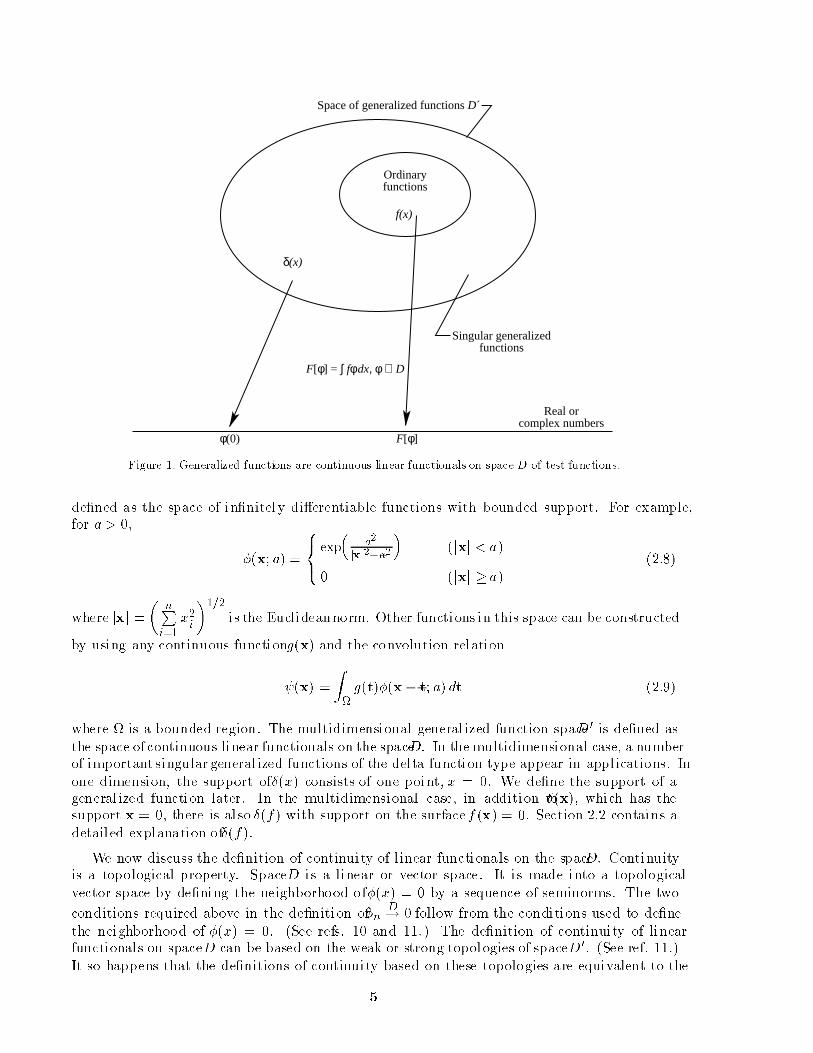
functionals on space D . The space of generalized functions on D is denoted D0. Figure 1 showsschematically how we extended the space of ordinary functions to generalized functions. We callordinary functions regular generalized functions, whereas all other generalized functions (such

as the Dirac delta function) are called singular generalized functions.

For algebraic manipulations, we retain the notation of ordinary functions for generalized

functions for convenience. We symbolically introduce the notation (x) for the Dirac deltafunction by the relation

[] = (0) =

Z(x)(x) dx (2:7)

Note that the integral on the right side of equation (2.7) does not stand for conventional

integration of a function. Rather, it stands for (0). We can now use (x) in mathematicalexpressions as if it were an ordinary function. However, we must remember that singulargeneralized functions are not, in general, dened pointwise; they dene a functional (i.e., a

function from our new point of view) when they are multiplied by a test function and appearunder an integral sign. Thus, when a singular generalized function appears in an expression, it

is always in an intermediate stage in the solution of a real physical problem.

More facts about space D in multidimensions, convergence to 0 in D, and the concept of

continuity of a functional are appropriate now. The multidimensional test function space D is

4

Ordinary functions

f(x)

δ(x)

Singular generalized functions

F[φ]φ(0)

F[φ] = ∫ fφ dx, φ ∈ D

Real or complex numbers

Space of generalized functions D´

Figure 1. Generalized functions are continuous linear functionals on space D of test functions.

dened as the space of innitely dierentiable functions with bounded support. For example,for a > 0,

(x; a) =

8<:

exp

a2

jxj2a2

(jxj < a)

0 (jxj a)

(2:8)

where jxj =

nPi=1

x2i

1=2

is the Euclideannorm. Other functions in this space can be constructed

by using any continuous functiong(x) and the convolution relation

(x) =

Zg(t)(x t; a) dt (2:9)

where is a bounded region. The multidimensional generalized function spaceD 0 is dened as

the space of continuous linear functionals on the spaceD. In the multidimensional case, a numberof importantsingulargeneralized functions of the delta function type appear in applications. In

one dimension, the support of(x) consists of one point, x = 0. We dene the support of ageneralized function later. In the multidimensional case, in addition to(x), which has thesupport x = 0, there is also (f) with support on the surface f (x) = 0. Section 2.2 contains a

detailed explanation of(f).

We now discuss the denition of continuity of linear functionals on the spaceD. Continuityis a topological property. SpaceD is a linear or vector space. It is made into a topological

vector space by dening the neighborhood of(x) = 0 by a sequence of seminorms. The two

conditions required above in the denition ofn ! 0D

follow from the conditions used to dene

the neighborhood of (x) = 0. (See refs. 10 and 11.) The denition of continuity of linearfunctionals on spaceD can be based on the weak or strong topologies of spaceD 0. (See ref. 11.)

It so happens that the denitions of continuity based on these topologies are equivalent to the

5

earl ier denition of F [n] ! 0 if and only if n ! 0D

. Furthermore, we note that because D is

a linear space, we can dene n ! D

if n ! 0D

and because F [ ] is linear, we can also say

that F [] is continuous if when n! D

, we have F [n ] ! F [] .

We conclude this discussion with one more important fact. Although in this paper we conne

ourselves to the test function space D, inmany applicationswe should use adierent test functionspace. For example, to dene Fourier transformation, we should use a test function space S of

innitely dierentiable functions that go to 0 at innity faster than jxjn for any n > 0 (thespace of rapidly decreasing functions). Other test function spaces are dened in Carmichaeland Mitrovic (ref. 10) and in references 12 and 13. Generalized functions on these spaces are

dened as continuous linear functionals after a suitable denition of convergence to 0 in thetest function space is given to get a topological vector space. Note that in all these spacesof generalized functions, the important singular generalized functions (such as the Dirac delta

function) are retained with properties essentially similar to those we study below in space D0.It can be shown that if A B and if A and B are two test function spaces used to dene

generalized function spaces A0 and B 0, respectively, then we have A B B 0 A0 (i.e. , the

space of generalized functions A 0 is larger than B 0). In particular, D S S 0 D0, where Sis the space of rapidly decreasing functions dened above.

2.2. How Can Generalized Functions Be Introduced in Mathematics?

Although Schwartz developed the theory of distributions, like many great ideas in mathe-matics and science, the subject has a long history. Synowiec (ref. 14) has stated that evolution

of the concepts of distribution theory followed a familiar pattern in mathematics of multiple andsimultaneous discoveries because the appropriate ideas were `in the air.' Several good sources onthe history of theory of distributions are available. (See refs. 15 and 16.) Therefore, we will not

present a detailed history here. Also, many dierent approaches in mathematics can be used tointroduce and develop systematically generalized function theory. We mention several of them

here.

2.2.1. Functional approach to generalized functions. In the functional approach, generalizedfunctions are dened as continuous linear functionals. This approach (which we use here) was

originally introduced by Schwartz (ref. 1) and is the most popular and direct method of studyinggeneralized functions. (See refs. 3, 4, and 7.) The operations on ordinary functions such asdierentiation and Fourier transformation are extended by rst writing these operations in the

language of functionals for ordinary functions, then by using them to dene the operations forall generalized functions. After the rules of these operations are obtained, the usual notation of

ordinary functions can be used for all generalized functions. A working knowledge is relativelyeasy to develop with this notation without confusion. Some elementary knowledge of functionalanalysis is needed in this approach.

2.2.2. Sequential approach to generalized functions. The sequential approach is essentiallybased on the original idea of Dirac in dening a delta function as the limit of a sequence ofordinary functions. The approach was originated by Mikusinski from a theorem in distribution

theory that the space of generalized functions is complete. Therefore, singular generalizedfunctions such as the delta function canbe dened as the limit of ordinary (i.e., regular) functions

much like dening irrational numbers as limits of a Cauchy sequence of rational numbers. Manygood books have been published on this subject. (See refs. 2, 6, and 17.) To dene a generalizedfunction, the analyst is required to construct and work with a sequence of innitely dierentiable

functions. Although mathematics only to the level of advanced calculus is involved, the algebraicmanipulations are technical and laborious. An extension to the multidimensional case also

appears more dicult than with the functional approach.

6

2.2.3. Bremermann approach to generalized functions. In the Bremermann approach,general ized functions of real variables are viewed as the boundary values of analytic functions on

the real axis. (See refs. 12 and 13.) The Bremermann approach has its basis in earlier works onFourier transformation in the complex plane to dene Fourier transforms of polynomials. This

approach employs some of the powerful results of analytic function theory and is particularlyuseful in Fourier analysis and partial dierential equations. A recent book on the subject is byCarmichael and Mitrovic. (See ref. 10.)

2.2.4. Mikusinski approach to generalized functions. The Mikusinski approach is based on

ideas from abstract algebra. A commutative ring is constructed from functions with supporton a semi-innite axis by dening the operations of addition and multiplication as ordinary

addition and convolution of functions, respectively. This commutative ring has no zero divisorsby a theorem of Titchmarsh. (See refs. 18 and 20.) Therefore, it can be extended to a eld bythe addition of a multiplicative identity and the multiplicative inverses of all functions. This

multiplicative identity turns out to be the Dirac delta function. The Mikusinski approach givesa rigorous explanation of the Heaviside operational calculus and solves other problems such as

the solution of recursion relations. One limitation of this approach is that the supports of thefunctions are conned to semi-axis or half-space in the multidimensional case. Good sourcesfor this approach are Mikusinski (ref. 18), Mikusinski and Boehme (ref. 19), and an excellent

expository book by Erdelyi (ref. 20)

2.2.5. Other approaches to generalized functions. Several other important approachesintroduce generalized functions in mathematics. One approach is based on the nonstandard

analysis of Robinson. (See ref. 21.) Nonstandard analysis uses formal logic theory to extendthe real line by the rigorous inclusion of Leibniz innitesimals. Many interesting applicationsof this theory, particularly in dynamical systems, are now available. Another more recent

approach is presented in Colombeau (refs. 22 and 23) and Rosinger (ref. 24). This approachuses advanced algebraic and topological concepts to develop a theory of generalized functions in

which multiplication of arbitrary functions is allowed and it is gaining popularity at present.Applications to nonlinear partial dierential equations are given by Rosinger (ref. 24) andOberguggenberger (ref. 25).

3. Some Denitions and Results

3.1. Introduction

In this section, some important denitions and results used later are presented. Then, the

generalized derivative, the multidimensional delta functions, and the nite part of divergentintegrals are discussed. This paper is application oriented so we are selective about the materialpresented here. We also freely refer to a generalized function by a symbolic or a functional

notation.

3.1.1. Multiplication of a generalized function by an innitely dierentiable function. Letf(x) be a generalized function in D 0 dened by the functional F [ ] and let a(x) be an innitely

dierentiable function. Then, a(x)f(x) is dened by the rule

aF [] = F [a] (3:1)

Note that aF stands for the functional that denes af . Also, because is in D , so is a. We

can use this denition to dene a(x)(x). Let [] be the Dirac function given by equation (2.6);then,

a [ ] = [a] = a(0)(0) (3:2)

7

Symbolically, this equation is interpreted as

a(x)(x) = a(0)(x) (3:3)

In the space D 0, multiplication of two arbitrary generalized functions is not dened; however,this statement needs clarication. Obviously, ordinary functions are also generalized functions

and any two ordinary functions can be multiplied; thus, they can also be multiplied in the senseof distributions. However, multiplication of a regular and a singular generalized function or two

singular generalized functions may not always be dened. For example, the multiplication of(x) by itself (i.e. , 2(x)) is not dened, neither is f(x)(x), where f(x) has a jump discontinuityor a singularity at x = 0. In applications, experience or inconsistencies in the results occasionally

show that some multiplications of two generalized functions are not allowed. Sometimes thisproblem can be removed by rewriting the expression such that the troublesome multiplication is

avoided. For example, diculties with multiplication of distributions appear if we use the masscontinuity and momentum equations in nonconservative forms to nd shock jump conditions(section 4.2). These diculties can be removed by using the conservation laws in conservative

forms. To overcome the problem of multiplication of distributions in space D 0, new spaces ofgeneralized functions have been dened. (See refs. 2327.) Colombeau (ref. 27, chapters 13)gives an intuitive description of the problem of multiplication of distributions and shows how to

remedy this problem.

3.1.2. Shift operator. Let f(x) be an ordinary function and dene the shift operator as

Ehf(x) = f(x + h). Then, if F [] is the functional representing f(x) by equation (2.1) and ifthe shifted function Ehf(x) is represented by EhF [] , we have

EhF [] =

Zf(x+ h)(x) dx

=

Zf(x)(x h) dx

= F [Eh ] (3:4)

This rule can now be used for all generalized functions in D0 because Eh is in D . For example,

Eh(x) = (x + h) has the property

Eh[] =

Z(x + h)(x)dx

= [(x h)]

= (h) (3:5)

Note that the integral in equation (3.5) is meaningless and stands for the functional Eh[],which in turn is given by [Eh].

3.1.3. Equality of two generalized functions f(x) and g(x) on an open set. Two generalized

functions f and g in D0 given by functionals F [] and G[ ] on D, respectively, are equal on an open set if F [] = G[] for all such that supp . For example, (x) = 0 on open sets

(0;1) and (1; 0). Note that generalized functions are compared only on open intervals.

3.1.4. Support of a generalized function. The support of a generalized function f(x) is thecomplement with respect to the real l ine of the open set on which f(x) = 0. For example, the

support of (x) is the set f0g; that is, the point x = 0.

8

3.1.5. Sequence of generalized functions. A sequence of generalized functions Fn [] isconvergent if the sequence of numbers fFn [ ]g is convergent for all in D. For example, let

n(x) =

8><>:n21n jxj

jxj 1

n

0jxj > 1

n

(3:6)

This function is shown in gure 2 and is, of course, an ordinary function. It can be shown that

limn!1

n(x) = (x) (3:7)

Thus, for the functional n[] representing n(x),

n [] =

Zn(x)(x) dx (3:8)

when is in D , we have

limn!1

n [] = (0)

= [] (3:9)

The index in the denition of convergence can be a continuous variable. For example, F"[] isconvergent as "! 0 if lim

"!0F"[] exists for all in D.

The following important theorem characterizes D0 and has signicant applications. (See

ref. 7.)

y

n

δn(x)

1 n– 1

n

Figure 2. Example of sequence.

9

Theorem: The space D0 is complete.

This theorem implies that a convergent sequence of generalized functions in D 0 always converges

to a generalized function in D 0.

We use this theorem later in this section whenwe discuss the nite part of divergent integrals.

3.1.6. Odd and even generalized functions. A generalized function F [] is even if F [(x)] =F [(x)] and odd if F [(x)] = F [(x)]. For example (x) is even and x is odd.

3.1.7. Derivative of a generalized function. The derivative of a generalized function is the mostimportant operation used in this paper. Let f (x) be an ordinary function with a continuous rstderivative (i.e. , f is a C1 function). If f(x) is represented by the functional F [] in equation (2.1),

then we naturally identify its derivative f 0(x) with F 0 [] given by the functional

F 0[] =

Zf 0dx (3:10)

Now we integrate by parts and use the fact that has compact support to get

F 0[] =

Zf 0dx

= F [0] (3:11)

Because 2 D, then 0 2 D . Thus, F [ 0] is a functional on D. We now use equation (3.11)to dene the derivative of all generalized functions in D 0. We can keep taking higher order

derivatives and obtain the following result:

F (n)[] = (1)nFh(n)

i(n= 1; 2; :: :) (3:12)

We have thus arrived at the following important theorem.

Theorem: Generalized functions have derivatives of all orders.

We have obtained a very surprising result. Even locally Lebesgue integrable functions that arediscontinuous are innitely dierentiable as generalized functions. What are the implications ofthis theorem in applications? We address this question about generalized derivatives and their

applications in section 3.2. First, some examples would be helpful.

Example 1. The derivative of the delta function 0(x) has the property,

0[] = [0]

= 0(0) (3:13)

Symbolically, we can write Z 0(x)(x) dx = 0(0) (3:14)

Note that 0(x) is an odd generalized function.

Example 2. The Heaviside function is dened as

h(x) =

1 (x > 0)

0 (x < 0)(3:15)

10

or in functional notation,

H [ ] =

Z 1

0(x)dx (3:16)

This function is discontinuous at x = 0. To dene the generalized derivative, we useequation (3.11) as follows:

H 0 [] = H [0]

=

Z 1

00 dx

= (0)

= [] (3:17)

Symbolically, we writeh0(x) = (x) (3:18)

Note the use of the bar over h0 to signify generalized dierentiation because h0(x) = 0 where

now h0 stands for the ordinary derivative.

We give one more important characterization of space D0 (ref. 7) known as the structuretheorem of distribution theory.

Theorem: Generalized functions in D 0 are generalized derivatives of a nite order of continuous

functions.

For example, we note that the Dirac delta function is the second generalized derivative of thecontinuous function

f(x) =

x (x 0)0 (x < 0)

(3:19)

3.1.8. Fourier transforms of generalized functions. We now work with the space of rapidlydecreasing test functions S . (See sec. 2.1, the last paragraph.) In this space the Fourier transform

of each test function is again in S . (See refs. 2, 4, 6, and 7.) We dene the Fourier transform ofan ordinary function (x) as b () = Z 1

1

(x)e2ix dx (3:20)

Let f(x) be an ordinary function that has the Fourier transform f() (e.g., let f be square

integrable on (1;1)). Then for (x) in S , the Parseval relation isZ 1

1

f(x) (x) dx =

Z 1

1

f (x)b (x) dx (3:21)

If now F [ ] is identied with f(x), then we should identify bF [ ] with f(). However,equation (3.21) is actually the relation

bF [ ] = F [b ] (3:22)

We use this relation as the denition of the Fourier transform of generalized functions in space

S 0. For example, b [ ] = [b ] = b (0) = Z 1

1

(x) dx (3:23)

11

The last integral is the functional generated by the function 1 so that

b() = 1 (3:24)

Thus, the Fourier transform of the Dirac delta function is the constant function 1.

We will not discuss this subject further because we do not use Fourier transforms extensively

in this paper. We note, however, that if is in D , then b is not necessarily in D andequation (3.22) is meaningless in D0 . Therefore, we must change the test function space fromD

to S . Another method of xing this problem is to use the Fourier transforms of functionsin space D as a new test function space bD. The Fourier transformations of functions inD0 are now continuous linear functionals on space bD . These generalized functions are called

ultradistributions. (See ref. 28.)

3.1.9. Exchange of limit processes. One of the most powerful results in generalized function

theory is that the limit processes can be exchanged. For example, all the following exchangesare permissible:

d

dx

Z =

Z

d

dx (3 :25a)

d

dx

Xn

=Xn

d

dx (3:25b)

Xn

Z =

Z

Xn

(3:25c)

limn!1

Z =

Z

limn!1

(3:25d)

d

dxlimn!1

= limn!1

d

dx (3:25e)

limn!1

Xm

=Xm

limn!1

(3:25f)

@2

@xi @xj =

@2

@xj @xi (3 :25g)

Here, as before, a bar over the derivative indicates generalized dierentiation. For example, letus consider the Fourier series of the simple periodic function with period 2

f(x) =

1 (0 < x < )

1 ( < x < 0)(3:26)

which is

f(x) =

1Xm=0

4

(2m + 1)sin(2m+ 1)x (3:27)

This function is shown in gure 3. The function f(x) has a jump of 2(1)n at x = n forn = 0; 1; 2. By a result given in section 3.2.1 (eq. (3.43)),

df

dx= 2

1Xn=1

(1)n(x n) (3:28)

12

1

0–π–2π π 2π x

–1

y

Figure 3. Periodic function with jump discontinuity of 2(1)n at x= n, n = 0;1;2;: : :.

Also, by equation (3.25b), we have

df

dx=

d

dx

1X

m=0

4

(2m + 1)sin(2m+ 1)x

=

1X

m=0

d

dx

4

(2m + 1)sin(2m+ 1)x

=

1X

m=0

4

cos(2m + 1)x (3:29)

From equations (3.28) and (3.29), we conclude that

2

1X

m=0

cos(2m+ 1)x=

1X

n=1

(1)n(x n) (3:30)

The series on the left is divergent in the classical sense. Nevertheless, such a result is often usefulin signal analysis. Another important application of exchange of limit processes is in obtaining

the nite part of a divergent integral. (See sec. 3.4.)

3.1.10. Integration of generalized functions. We say that G[] is an integral ofF [ ] if

G0[ ] = F [] (3:31)

For example, we can easily show that the Heaviside function is an integral of the Dirac deltafunctionbecause

H 0 [] = H [0]

= (0)

= [] (3:32)

Let K [] be a generalized function such that

K 0 [] = 0 (3:33)

13

for all 2 D. Then, if G[] is an integral of F [], it follows that (G+ K)[] = G[ ] +K [] isalso an integral of F [] . References 7 and 29 show that the only solution of equation (3.33) in

D0 is

K [] =

Zc(x) dx (3:34)

where c is an arbitrary constant (i.e., K [] is a constant distribution). This result correspondsto the classical indenite integration of a functionZ

f(x)dx = g(x)+ c (3:35)

We use the same notation symbolically for all generalized functions. For example, we writeZ(x) dx = h(x) + c (3:36)

where h(x) is the Heaviside function. Note that the integral on the left of equation (3.36) ismeaningless in terms of the classical integration theories.

3.2. Generalized Derivative

The generalized dierentiation concept is quite important in generalized function theory;

this section focuses on it and gives some very useful results for applications. Indeed, the resultsthemselves, rather than the mathematical rigor used in deriving them, are of interest in thispaper. As before, a bar over the dierentiation symbol denotes generalized derivatives if there

is an ambiguity in interpretation. For example, we use df=dx, f 0(x), @f=@xi , and @2f=@xi @xj

to denote generalized derivatives of ordinary functions, but we do not use a bar over 0(x) and@(f)=@xi because it is obvious that these derivatives can only be generalized derivatives because(x) and (f ) are singular generalized functions.

3.2.1. Functions with discontinuities in one dimension. Let f(x) be a piecewise smoothfunction with one discontinuity at x0 with a jump at this point dened by the relation

f = f(x0+) f(x0) (3:37)

We want to nd the generalized derivative of f (x). Let be in D and let x0 be in the

support of (x). Then if F [] is the functional representing f(x) by equation (2.1), we have forsupp = [a; b ], the result

F 0 [] = F0

=

Z b

af (x)

0

(x) dx

=

"Z x0

a+

Z b

x0+

f(x)0(x)dx

#

=

Z b

af 0(x)(x)dx+ [f(x0+) f (x0)](x0)

=

Z b

af 0(x)(x)dx+ f (x0) (3:38)

14

We have performed an integration by parts to get to the last step. We have also used the fact that(a) = (b) = 0 in the integration by parts. Noting that (x0) = [ (x + x0)] = Ex0

[(x)],

where Ex0 is the shift operator, we write equation (3.38) symbolically as

f0(x) = f 0(x)+ f (x x0) (3:39)

One question is the use of f 0(x) compared with the ordinary derivative f 0(x). Let us studyequation (3.38). The functional F 0[] corresponding to f 0(x) indeed has retained the memory of

the jump f on the right side of the equation. Symbolically, f 0(x) can be integrated over [c; x],where c < x0 < x, to give the result

f(x) =

Z x

cf 0(x)dx + f(c)+ fh(x xo) (3:40)

Thus, we have recovered the original discontinuous function. We note, however, that

f(x) 6=

Z x

cf 0(x)dx + f(c) (3:41)

because the memory of the jump f is not retained in f 0(x) but is retained in f 0(x). If a

function f (x) has n discontinuities at xi; i = 1 n with the jump fi at xi dened by

fi = f(xi+) f(xi) (3:42)

then

f 0(x) = f 0(x) +

nXi=1

fi (x xi) (3:43)

This equation is the rst indication that when we work with discontinuous functions inapplications, the proper setting for the problem is in the space of generalized functions. In

particular, if an integral method, such as the approach that uses the Green's function, is usedto nd the solution, essentially no signicant changes to algebraic manipulations are needed in

nding discontinuous solutions provided we stay in the space of generalized functions. Again,we will have more to say about this later. (See sec. 3.2.3.)

3.2.2. Functions with discontinuities in multidimensions. Let us now consider the functionf(x), which is discontinuous across the surface g(x) = 0. Let us dene the jump f across

g = 0 by the relation

f = f(g = 0+) f(g = 0) (3:44)

Note that g = 0+ is on the side of the surface g = 0 into which rg points. We would like to

nd @f=@xi . To do this we use the results from section 3.2.1 as follows. Let us put a surfacecoordinate system

u1; u2

on g = 0 and extend the coordinates to the space in the vicinity of

this surface along normals. Let u3 = g be the third coordinate variable that is well dened by

the function g in the vicinity of this same surface. We note that f in variables u1 and u2 iscontinuous, but it is discontinuous in variable u3. Therefore, we have

@f

@ui=

@f

@ui(i = 1; 2) (3 :45a)

@f

@u3=

@f

@u3+ f (u3) (3:45b)

15

In equation (3.45b), we used equation (3.39). Thus, using the summation convention on indexj , we get

@f

@xi=

@f

@uj

@uj

@xi

=@f

@uj

@uj

@xi+ f

@u3

@xi(u3)

=@f

@xi+ f

@g

@xi(g) (3:46)

We can write this in vector notation as

rf =rf + frg (g) (3:47)

In section 3.2.3, we discuss how to interpret (g) when g = 0 is a surface. We can simi larly

dene generalized divergence and curl as follows:

r f = r f +rg f (g) (3 :48a)

r f = r f +rg f (g) (3:48b)

The rigorous derivation of both these results requires some knowledge of the invariant denition

of divergence and curl in general curvilinear coordinate systems. (See refs. 8 and 9.) We cancombine the above three results by using for the three operations such that

r f = r f + rg f (g) (3:49)

3.2.3. Ordinary dierential equations and Green's function. We give a few simple results

here. One important question discussed in connection with integrals of generalized functions isthe solution of

f0(x) = 0 (3:50)

in D 0. It can be shown easily that the only solution of this equation is the classical one (refs. 7

and 29)

f(x) = C (3:51)

where C is a constant. However, the solution of the equation

xf(x) = 0 (3:52)

which is not a dierential equation, is

f(x) = C(x) (3:53)

To get this solution, some simple results from the generalized Fourier transform are used. (Seeref. 29.) Taking the Fourier transform of both sides of equation (3.52), we get

d

df () = 0 (3:54)

16

Therefore, after integration of equation (3.54), we have

f () = C (3:55)

By taking the inverse Fourier transform of both sides of equation (3.55), we get equation (3.53).

From this result, the solution ofxf 0(x) = 1 (3:56)

is found asf(x) = lnjxj + C1 + C2h(x) (3:57)

where C1 and C2 are constants and h(x) is the Heaviside function. The solution C2h(x) comesfrom the fact that the generalized function f 0(x) satisfying the equation

xf 0(x) = 0 (3:58)

is, from equation (3.53),f 0(x) = C2(x) (3:59)

Thus, the solution of the homogeneous equation (3.58) is the integral of this function

f(x) = C1 + C2h(x) (3:60)

Let us now consider a second order linear ordinary dierential equation with two linear and

homogeneous boundary conditions (BC) as follows:

`u = A(x)u00 + B(x)u0 + C(x) = f(x)BC1[u] = 0BC2[u] = 0

9=;

(x 2 [0; 1])(3:61)

Let us also assume that we know u is a C1 function and u00 is Lebesgue integrable so that u00 = u00

and u0 = u0. Suppose a function g(x; y) exists, the Green's function, such that

u(x) =

Z 1

0f(y)g(x; y)dy (3:62)

Because u 2 C1, then u = `u by continuity of u and u0. We know we can take into theintegral in equation (3.62) but not ` because g(x; y) may not belong to C1. Therefore, using `xto indicate that derivatives in ` are with respect to x, we get

`u = u

= x

Z 1

0f(y)g(x; y)dy

=

Z 1

0f(y)xg(x; y)dy

= f(x) (3:63)

from equation (3.61). We see that xg(x; y) must have the sifting property

xg(x; y) = (x y) (3:64)

17

Because the BC's are linear, we also have

BC[u] =

Z 1

0f(y)BCx[g(x; y)] dy (3:65)

Therefore, other conditions on g(x; y) are

BC1x[g(x; y)] = 0 (3 :66a)

BC2x[g(x; y)] = 0 (3:66b)

where the x in the subscripts of the BC's indicates that g(x; y) in the variable x satises the twoboundary conditions.

From equation (3.64) we conclude that, because x is a second order ordinary dierential

equation, g(x; y) must be continuous at x = y and @g=@x must have a jump discontinuity at

x= y . The reason is that if g(x; y) has a discontinuity at x= y, the rst generalized derivativewith respect to x will give a (x y) by equation (3.39). A second generalized derivative wouldgive 0(x y) in the result. But because 0(x y) is missing on the right of equation (3.64),

g(x; y) cannot be discontinuous at x= y. Assuming that g(x; y) is dened by

g(x; y) =

(g1(x; y) (0 x < y)

g2(x; y) (y < x 1)

(3:67)

equation (3.64) means that

`xg1(x;y) = `xg2

(x; y) = 0 (3 :68a)

g1(y; y) = g

2(y; y) (3:68b)

@ g2

@x(y; y)

@g1

@x(y; y) =

1

A(y)(3:68c)

Note that equation (3.68a) is the same as `xg = 0 used above. This equation means that g1and

g2in variable x are solutions of the homogeneous equation `u = 0. Equation (3.68b) expresses

continuity of g at x = y and equation (3.68c) gives the jump of @g=@x at x = y. To get

equation (3.68c), we note that

xg = `xg + A(y)

@g

2

@x(y; y)

@g1

@x(y; y)

(x y)

= A(y)

@g

2

@x(y; y)

@g1

@x(y; y)

(x y)

= (x y) (3:69)

The last delta function follows from equation (3.64). Equation (3.68c) follows from the fact thatthe coecient of (x y) in the expression after the second equality sign must be equal to 1.The Green's function is now determined from equations (3.66) and (3.68ac).

3.2.4. Leibniz rule of dierentiation under the integral sign. We want to nd the result of

taking the derivative with respect to variable in the following expression in which A, B , and

18

f are continuous functions and B() > A() for 2 [a; b]. Thus,

E() =d

d

Z B()

A()f(x; ) dx (3:70)

Let us dene the function H(x; ) as follows:

H(x; ) = h[x A()]h[B() x] (3:71)

where h(x) is the Heaviside function. The function H(x; ) = 1 when A() < x < B() and

H(x; ) = 0 otherwise. Using H(x; ), we can write E() as

E() =d

d

Z1

1

H (x; )f(x; ) dx

=

Z1

1

@H

@f + H

@f

@

dx (3:72)

We have

@H

@(x; ) = A0()h[B() x] [x A()]

+ B 0()h[x A()] [B() x]

= A0()[x A()] + B 0() [B() x] (3:73)

Note that we have used

h[B() x] [x A()] = h[B() A()][x A()]

= [x A()] (3:74)

because B() A() > 0; thus, the Heaviside function is 1. Similarly, we do the same as inequation (3.74) for the secondproduct of the Heaviside and the delta functions in equation (3.73).

Using equation (3.73) in equation (3.72) and integrating with respect to x, we get the Leibnizrule of dierentiation under the integral sign,

E() =

Z B()

A()

@f

@(x; ) dx + B 0()f [B(); ] A0()f [A(); ] (3:75)

3.3. Multidimensional Delta Functions

In multidimensions, (x) has a simple interpretation given by

Z(x)(x) dx = (0) (3:76)

Thus,

(x) = (x1)(x2) : : : (xn) (3:77)

where x = (x1; x2 ; : : : ; xn). In this section, we conne ourselves to three-dimensional space. Of

interest in applications are (f) and 0(f) where f = 0 is a surface in three-dimensional space.

19

We can always assume that f is dened so that jrf j = 1 at every point on f = 0. If f does nothave this property, then f1 = f= jrf j does. Thus, redene the surface.

3.3.1. Interpretation of (f ). Consider the integral

I =

Z(x)(f) dx (3:78)

Assume that we dene a curvilinear coordinate systemu1 ; u2

on the surface f = 0 and extend

these variables locally to the space near this surface along local normals. Let u3 = f which,

because jrf j = df=du3 = 1, u3 is the local distance from the surface. Thus, f = u3 = constant6= 0 is a surface parallel to f = 0. Of course, we assume u3 is small. From dierential geometry

(refs. 8 and 9), we have

dx =q

g(2)

u1; u2 ; u3

du1du2 du3 (3:79)

where g(2)u1; u2; u3

is the determinant of the rst fundamental form of the surface f = u3 =

Constant. Using equation (3.79) in equation (3.78) and integrating with respect to u3 gives

I =

Z

hx

u1; u2; u3

i

u3q

g(2)u1; u2; u3

du1du2du3

=

Z

hx

u1; u2; 0

iqg(2)

u1 ; u2 ; 0

du1 du2

=

Zf=0

(x)dS (3:80)

That is, I is the surface integral of over the surface f = 0.

3.3.2. Interpretation of 0(f). We want to interpret

I =

Z(x) 0(f) dx

=

Z

hx

u1 ; u2 ; u3

i0u3 q

g(2)u1 ; u2 ; u3

du1 du2 du3 (3:81)

Here we have used the coordinate systemu1 ; u2 ; u3

dened above. Integrating the above

equation with respect to u3 gives

I =

Z@

@u3

h(x)

qg(2)

u1 ; u2 ; u3

iu3=0

du1 du2 (3:82)

Again, from dierential geometry, we have

@

@u3

qg(2)

u1 ; u2 ; u3

= 2Hf

u1 ; u2 ; u3

qg(2)

u1; u2; u3

(3:83)

20

where Hf stands for the local mean curvature of the surface f = u3 = Constant. Taking thederivative of the integrand of equation (3.82) and using the result of (3.83), we obtain

I =

Z@

@u3

hx

u1 ; u2 ; 0

iqg(2)

u1 ; u2; 0

du1du2

+

Z2Hf

u1; u2; 0

hx

u1 ; u2 ; 0

iqg(2)

u1; u2; 0

du1du2

=

Zf=0

@

@n+ 2Hf(x)(x)

dS (3:84)

where @=@n is the usual normal derivative of . Intuitively, the appearance of the term 2Hf

in the integrand is not at all obvious. This appearance is a clear indication of the importanceof dierential geometry in multidimensional generalized function theory.

3.3.3. A simple trick. We have already shown that (x)(x) = (0)(x). By taking thederivative of both sides of this equation, we get

0(x)(x)+ (x) 0(x) = (0)0(x) (3:85)

Obviously, the right side is simpler than the left side. Let us consider the expression

E = (x)(f) =

hx

u1 ; u2 ; u3

i

u3

(3:86)

where again we have used the coordinate systemu1 ; u2 ; u3

dened in section 3.3.1 above. We

know that

hx

u1 ; u2 ; u3

i

u3=

hx

u1 ; u2 ; 0

i

u3

(3:87)

We use the notation~(x) for

x

u1 ; u2 ; 0

; that is,

~(x) is the restriction of

~(x) to the support

of the delta function that is the surface f = 0. We note that @~=@n =

@=@u3

xu1 ; u2 ; 0

= 0. Using

~(x), we can write E in two forms:

E = (x)(f ) (First form)

E = ~(x)(f ) (Second form)

9=; (3:88)

Is there an advantage of using the second form compared with the rst form? The answer isyes! Let us take the gradient of E for the two forms in equation (3.88). Thus,

rE = r (f) + (x) rf 0(f) (First form)

rE = r2~(f)+

~(x)rf 0(f) (Second form)

9>=>; (3:89)

Here, r2~is the surface gradient of

~(x) on f = 0. From equation (3.84), we note that

in the integration of 0(f) in the rst form, the term @=@n cancels a similar term in the in-

tegration of r (f). In the second form, because @~=@n = 0, @

~=@n does not appear in

the integration of 0(f ) and obviously is also absent in the integration of r2~(f). Therefore,

21

algebraic manipulations are reduced. It is, thus, expedient to restrict functions multiplyingthe Dirac delta function to the support of the delta function. Note carefully that functions

multiplying 0(x) cannot be restricted to the support of 0(x); that is, (x) 0(x) 6= (0) 0(x).

3.3.4. The divergence theorem revisited. Let be a nite volume in space and let (x) be aC1 vector eld. Let us dene the discontinuous vector eld 1(x) as

1(x) =

((x) (x 2 )

0 (x 62 )(3:90)

Let the surface f = 0 denote the boundary @ of region in such a way that n = rf points tothe outside of @ and jrf j = 1 on f = 0. We have

r 1 = r 1 + 1 n (f )

= r 1 (x) n (f) (3:91)

We note that 1 = 1(f = 0+) 1(f = 0) = (f = 0). Integrating over the unbounded

three dimensional space, we get

Z Z Z@1;1

@x1dx1 dx2 dx3 =

Z Z1

11

dx2 dx3 = 0 (3:92)

Similarly, we get zero for integrals of @1;2=@x2 and @1;3=@x3, where 1;i is the ith component

of 1. Therefore, Zr 1 dx = 0 (3:93)

Now, the integration of the right side of equation (3.91) using equation (3.80) gives

Zr dx

Z@

n dS = 0 (3:94)

Here we have used the fact that, from equation (3.90),

r 1 =

(r (x 2 )

0 (x 62 )(3:95)

Also, we dene n = n. Equation (3.94) is the divergence theorem.

We note that equation (3.93) is valid if 1 has a discontinuity across the surface k = 0 within as shown in gure 4. Equation (3.94) is therefore valid ifr in the volume integral is replaced

by r , where the only jump of in the generalized divergence comes from the discontinuityon k = 0. That is, we write

r = r + n0 (k) (3:96)

where n0 = rk is the unit normal to k = 0. Equation (3.94) can now be written

Zr dx =

Z@

n dS (3:97)

22

∇k = n´

n

∂Ω

k = 0

Ω

Sk

Figure 4. Control volume intersecting surface of discontinuity of vector eld used for deriving generalized

divergence theorem.

which, by using equation (3.96),we can also write as

Zr dx =

Z@

n dS

ZSk

n0 dS (3:98)

where n0 = n0 and Sk is the part of the surface k = 0 enclosed in region . (See g. 4.)

The divergence theorem is used in deriving conservation laws in uid mechanics and physics

in dierential form. The fact that it remains valid for discontinuous vector elds, as shownin equation (3.97), implies that such conservation laws are valid when all the derivativesare interpreted as generalized derivatives. Thus, the jump conditions across the surface of

discontinuities are inherent in these conservation laws as shown in section 3.4. This interpretationof conservation laws eliminates the need for the pillbox analysis of jump conditions.

3.3.5. Product of two delta functions. We have said earlier that the product of two arbitrarygeneralized functions generally may not be dened. Here we give the interpretation of theproduct of two multidimensional generalized functions for which multiplication is possible. Let

f = 0 and g = 0 be two surfaces intersecting along a curve as shown in gure 5. Assumerf = n and rg = n

0 , where jnj = jn0 j = 1. We want to interpret

I =

Z(x)(f )(g) dx (3:99)

On the local plane normal to the -curve, deneu1 = f , u2 = g, and u3 = , where is thedistance along the -curve. Extend u1 and u2 to the space in the vicinity of the plane along alocal normal to the plane. We have

dx =du1 du2 du3

sin(3 :100)

23

∇g = n'

f = 0

∇f = n

g = 0

Γ

Figure 5. Integration of (f) (g) for two intersecting surfaces f = 0 and g= 0.

where sin = jn n0j. Using equation (3.100) in equation (3.99) and integrating the resultingintegral with respect to u1 and u2, we get

I =

Z(x)

sin

u1

u2du1du2 du3 =

Zf=0g=0

(x)

sind (3 :101)

This result is useful in applications. (See sec. 4.3.)

3.4. Finite Part of Divergent Integrals

The nite part of divergent integrals is important in aerodynamics. The classical procedure

for nding the nite part of divergent integrals appears ad hoc and leads to questions about thevalidity of the procedure. First, could the appearance of divergent integrals in applications bethe result of errors in modeling the physics of the problem? Second, will the method lead to a

unique analytical expression or do dierent analytical expressions lead to equivalent numericalresults? The generalized function theory clearly answers these questions.

Let us rst examine the function f(x) = lnjxj , which is locally integrable. The ordinaryderivative of this function is

d

dxlnjxj =

1

x(3 :102)

which is not locally integrable over any interval that includesx = 0. We know, however, thatas a generalized function, lnjxj has generalized derivatives of all orders. What is the relation ofthe generalized derivative of lnjxj to the ordinary derivativef 0(x) = 1=x?

Let us work with F [] representing lnjxj as follows:

F [] =

Zlnjxj(x) dx ( 2 D) (3 :103)

We have, using the denition of generalized derivative,

F 0[ ] =

Zlnjxj 0(x)dx (3 :104)

24

hε(x)

1

–ε αε

Figure 6. Function h"(x) used in dening nite part of divergent integralR[(x)=x]dx. "> 0; > 0.

We need some integration by parts to get the term 1=x in the integrand of equation (3.104).

However, this integration cannot be performed because 1=x is not locally integrable. We solvethis problem by using a new functional depending on", the limit of which isF 0[] as follows.

Let h"(x) be a function dened below for some constant > 0 and a parameter " > 0. Thus,

h"(x) =

(0 (" < x < ")

1 (Otherwise)(3 :105)

This function is shown in gure6. Then it is obvious that lnjxj can be written as the limit of

an indexed generalized function as follows:

lim"!0

h"(x)lnjxj = lnjxj (3 :106)

Note that if we dene F 0"[] as

F 0"[] =

Zh"(x)lnjxj

0(x) dx (3 :107)

then we have from the completeness theorem ofD0 (sec. 3.1.5)

lim"!0

F 0"[] = F 0[] (3:108)

The function h"(x)lnjxj has two jump discontinuities atx = " and x = ". We can eitherapply the classical integration by parts to equation (3.107) by breaking the real line into twointervals or by using the generalized derivative

F 0"[] =

Z d

dx[h"(x) lnjxj](x) dx (3 :109)

Here we are integrating oversupp and we do not worry about the terms coming from the limitsof the integral in the integration by parts because = 0 at the limit points.

We now take the derivative of the term in square brackets in equation (3.109):

d

dx[h"(x)lnjxj] =

h"(x)

x ln"(x + ") + ln(")(x ") (3 :110)

25

Here and below, we have used the result that (x) (x x0) = (x0) (x x0). Thus, afterusing equation (3.110) in equation (3.109) and integrating with respect to x, we have

F 0"[] = ln "(") + ln(")(") +

Zh"(x)

x(x) dx

= (0)ln+

Zh"(x)

x(x)dx+ o(") (3 :111)

where o(") stands for terms of order " and higher. Now from equation (3.108) we have

F 0[ ] = lim"!0

F 0"[]

= (0)ln+ lim"!0

Zh"(x)

x(x) dx

= (0)ln+ lim"!0

Z "

1

(x)

xdx +

Z 1

"

(x)

xdx

(3 :112)

We can show that the limit of the integral on the right of equation (3.112) exists. If now = 1,

then ln = 0 and

F 0 [] = lim"!0

Z"

1

(x)

xdx+

Z1

"

(x)

xdx

(3 :113)

which is known as the Cauchy principal value (PV) of the integral. But = 1 need not be takenand equation (3.112) is numerically the same as equation (3.113). The above limit procedure iscalled taking the nite part of a divergent integral.

What have we achieved? Over any open interval that does not include x = 0 we have

d

dxlnjxj =

1

x(3 :114)

but when x = 0 belongs to the open interval, then the classically divergent integral must

be interpreted such that the functional F 0[] corresponding to (d=dx) lnjxj is recovered. Asthe above simple function demonstrates, more than one dierent analytical expression for theprocedure can be used to nd the nite part of a divergent integral. However, all the expressions

are numerically equivalent. We dene the principal value of 1=x as

PV

1

x

=

d

dxlnjxj (3 :115)

Thus, when x = 0 is in the interval of integration of 1=x, the nite part of the divergent integralmust by taken to get the numerical value of F 0[] , where F [] is given by equation (3.103). Note

that the term regularizing a divergent integral is also used in mathematics. The procedure givenhere corresponds to the canonical regularization of Gel 'fand and Shilov. (See ref. 7.)

What is the use of this procedure in applications? Suppose we have reduced the solution of

a problem to the evaluation of the expression

u(x) =d

dx

Z(y) lnjx y j dy (3 :116)

26

where x 2 . Let us assume that we know that the integral is continuous as a function of x sothat d=dx can be replaced by d=dx and taken inside the integral. We get

u(x) =

Z(y)

d

dxlnjx yj dy

=

Z(y)PV

1

x y

dy (3 :117)

which is interpreted as the nite part of the divergent integral by the procedure dened earlier.

We remind the readers that the procedure will result in exactly what equation (3.116) wouldgive had we been able to perform the integration analytically. Also, assuming that = 0 at the

boundaries of , an integration by parts of the rst integral in equation (3.117) would give

u(x) =

Z0(y)lnjx yj dy (3 :118)

which is also a legitimate result if this integral exists. The problem is that often in applications,equation (3.116) is an integral equation for the unknown function (x), which has integrable

singularities at the boundaries of the interval . Thus, the above integration by parts is invalidand, in any case, the integral equation (3.118) is divergent. Therefore, the only choice left isthe integral equation with the principal value of 1=(x y), which is a well-known kernel in the

theory of singular integral equations.

We now give an advanced example in three dimensions with a surprising implication in thenumerical solution of an integral equation of transonic ow which we will discuss in section 4.

Let us consider the integral

I(x) =@2

@x21

Z

(y)

rdy (3 :119)

r2 = (x1 y1)2 + (x2 y2)

2 + (x3 y3)2 (3 :120)

where is a region in space and x 2 . In this problem (x) is a C1 function and is theunknown of the aerodynamic problem. Assuming that the integral is a C1 function in x, we can

replace @2=@x21 with @2=@x21 and take the derivatives inside the integral

I(x) =

Z(y)

@2

@x21

1

r

dy

=

Z(y)

@2

@y21

1

r

dy (3 :121)

We use generalized dierentiation rather than ordinary dierentiation because the latter willresult in a divergent integral. Note that

@

@y1

1

r

=

r1r3

(3:122a)

@2

@ y21

1

r

=

3r21 r2

r5(3:122b)

27

where r1 = x1 y1. Because r1=r3 is integrable, we write

@2

@y21

1

r

=

@

@y1

r1r3

(3 :123)

and we proceed to nd the nite part of the divergent integral in equation (3.121).

Let f(y ;x; ") = g (r1; r2 ; r3) " = 0 be a piecewise smooth surface enclosing the pointy = x where ri = xi yi , i = 13 and g is a homogeneous function of order 1; that is,

g (r1 ; r2 ; r3) = g (r1 ; r2; r3). This condition assures that the surface g (r1 ; r2 ; r3)" = 0corresponds to g (r1 ; r2 ; r3) "= = 0 for 6= 0. Thus, all the surfaces g " = 0 correspondto various values of that are similar in shape. From the homogeneity of g, it follows that

f(y ;x; 0) = g (r1; r2 ; r3) = 0 consists of a single-point y = x. For example, for a sphere with acenter at y = x and radius ", we have

f(y ;x; ") =

qr21 + r22 + r23 " = 0 (3 :124)

In addition, we assume ryf = n, where n is the local unit outward normal to the surface. Let

f > 0 outside and f < 0 inside this surface, respectively. We introduce the function h"(y) bythe relation

h"(y) =

(1 (f > 0)

0 (f < 0)(3 :125)

Now, we dene the required generalized derivative in equation (3.123) by the relation

@2

@y21

1

r

= lim

"!0

@

@y1

h"(y)r1

r3

= lim"!0

"r1n1

r3(f)+

3r21 r2

r5h"(y)

#(3 :126)

where n1 is the component of n along the y1-axis. Therefore, I(x) can be written

I(x) = lim"!0

Zf=0

r1 n1

r3(y) dS

+ lim"!0

Z

3r21 r2

r5h"(y)(y)dy (3 :127)

where we have used equation (3.80) to integrate (f ) in equation (3.126).

Using a Taylor series expansion of (y) at y = x , we nd that

lim"!0

Zf=0

r1 n1r3

(y) dS = f (x) (3 :128)

where f is a constant depending on the shape of the surface f = 0. For example, for the spheregiven by equation (3.124), we have

f =4

3(3 :129)

28

If we take the surface f = 0 to be a circular cylinder with its axis parallel to the y1-axis suchthat the base radius is " and its height is ; "

1, then

f = 4 (3 :130)

Equation (3.127) is thus written

I (x) = f (x) + lim"!0

Z

3r21 r2

r5h"(y)(y)dy (3 :131)

Numerically, I (x) is the same regardless of the shape of f = 0. Because3r21 r2

=r5 near y = x

takes both positive and negative values, the shape of f = 0 as " ! 0 aects the value of theintegral in the summation process. This eect is similar to a well-known result for conditionallyconvergent series, which can be made to converge to any value by rearranging the terms of the

series. The term f(x) in equation (3.131) compensates for the change in the value of thevolume integral when f = 0 is changed so that I(x) is numerically the same.

What is the implication of the above result in applications? In practice, the volumeintegration is performed numerically. The volume integral has a hole enclosing y = x whoseboundary surface is given by f = 0. The value of f must, therefore, correspond to the grid

system used in the volume integration. If the hole is rectangular, which is often the case, thenneither of the above two f 's in equations (3.129) and (3.130) is appropriate for the problem.

One question remains unanswered. When does the appearance of a divergent integral implyanything other than the breakdown of the physical modeling? The answer is when we have

wrongly taken an ordinary derivative inside an improper integral. Such a step can make theintegral divergent and is caused by the wrong mathematics (improper procedure) rather than thewrong physics. Thus, the analyst should always check the cause of the appearance of divergent

integrals in applications. Because in classical aerodynamics, the inappropriate mathematicsgenerally causes the appearance of divergent integrals, the nite part of divergent integrals must

be used.

4. Applications

4.1. Introduction

In this section we give some applications in aerodynamics and aeroacoustics that show

the power and the beauty of generalized function theory. We use the results of the previoussections here. Many areas of aerodynamics and aeroacoustics can use generalized functiontheory, especially because the approach is almost always more direct and simpler than other

methods. In addition, for many problems involving partial dierential equations, no alternatemethod is available for nding a solution. Below is a partial list of applications of generalized

function theory in aerodynamics, uid mechanics, and aeroacoustics:

Aerodynamics and uid mechanics

Derivation of transport theorems

Derivation of governing conservation laws (such as two-phase ows)

Derivation of jump conditions across ow discontinuities, velocity discontinuity as a vortexsheet

Derivation of the governing equation for boundary element or eld panel methods

Subsonic, transonic, and supersonic aerodynamic theory

29

Aeroacoustics

Sound from moving singularities

Derivation of the governing equation for the boundary element method

Derivation of the Kirchho formula for moving surfaces

Study of noise from moving surfaces using the acoustic analogy

Identication of new noise generation mechanisms and their source strength (such as shock

noise)

In addition, in both aerodynamics and aeroacoustics, generalized function theory can help in

the derivation of geometric identities involving curves, surfaces, and volumes, particularly underdeformation and in motion.

4.2. Aerodynamic Applications

We give here four applications that have been previously derived by other classical methods.

The method based ongeneralized function theory, as expected, is much shorter and more elegant.Other examples in aerodynamics are presented by De Jager. (See ref. 5.)

4.2.1. Two transport theorems. We give two results here that are used in the derivation of

conservation laws. We want to take the time derivative inside the integral

I =d

dt

Z(t)

Q(x; t)dx (4:1)

where (t) is a time-dependent region of space and Q(x; t) is a C1 function. Let us assume the

boundary @(t) of is piecewise smooth and is given by the surface f = 0 such that f > 0 in. Assume also that rf = n0 where n0 is the unit inward normal to the surface. Suppose wecan ascertain that the integral in equation (4.1) is continuous in time. Then, we can replace

d=dt with d=dt and bring the derivative inside the integral. We write

I =d

dt

Zh(f )Q(x; t)dx

=

Z @f

@ t(f)Q(x ; t)+ h(f)

@Q

@t

dx

=

Z@(t)

@f

@tQ(x; t) dS +

Z(t)

@Q

@tdx (4:2)

where h(f ) is the Heaviside function. Here we have used equation (3.80) to integrate (f) in the

second step above. We can show that

@ f

@t= vn0 = vn (4:3)

where vn0 and vn are the local normal velocities in the direction of inward and outward normals,respectively. Thus,

I =

Z@(t)

vnQ(x; t) dS +

Z(t)

@Q

@tdx (4:4)

This equation is the generalization of the Leibniz rule of dierentiation of integrals in one

dimension.

30

For the second result, we want to take the time derivative inside the following integral byassuming again that the integral is continuous in time and that Q is a C1 function. Thus,

I =d

dt

Z@(t)

Q(x ; t) dS (4:5)

We rst convert the surface integral into a volume integral

I =d

dt

Z(f)Q

~(x; t) dx (4:6)

Here f = 0 describes @(t) and rf = n, where n is the unit outward normal. Also, note thatQ~is the restriction of Q to f = 0 as explained in section 3.3. Therefore,

I =

Z 24@f@t

0(f)Q~(x ; t) + (f )

@Q~

@t

35dx (4:7)

We now must use the results of section 3.3 to integrate 0(f) and (f ). However, @f=@t = vn~

and this function is restricted already to f = 0. Thus,

@

@n

vn~

Q~(x ; t)

= 0 (4:8)

Using equations (3.80) and (3.84), we get

I =

Z@(t)

24 @Q

~@t

2vnHfQ(x ; t)

35dS (4:9)

where Hf is the local mean curvature of @(t). What is @Q~=@t? We have the following result,

assuming that Q is nonimpulsive,

@Q~

@t=

@Q

@t+ vn

@Q

@n(4:10)

Derivation of equation (4.9) by other methods is not trivial.

4.2.2. Unsteady shock jump conditions. These conditions are usually obtained by the pillboxanalysis. We present a method here based on generalized function theory. We have said thatthe conservation laws such as the mass continuity and the momentum equations are valid as

they stand if we replace all ordinary derivatives with generalized derivatives. We derive here thejump conditions from these two conservation laws. Let k(x; t) = 0 describe an unsteady shock

surface. Let rk = n, where n is the unit normal pointing in the downstream direction. Wedenote this downstream region as region 2 and the upstream region as region 1. We dene thejump Q in any parameter by

Q = [Q]2 [Q]1 (4:11)

31

∇ × u = 0∇k = n

k(x) = 0

WakeWing

Figure 7. Thin wing in incompressible, irrotational ow with wake.

where the subscripts 1 and 2 refer to the upstream and downstream regions, respectively.

Applying the rules of generalized dierentiation to the mass continuity equation, we have

@

@t+r (u) =

@

@t+r (u)

+

@k

@t+ (u) n

(k) = 0 (4:12)

where is the density andu is the uid velocity. The sum of the rst two terms on the right of

the rst equality sign is the ordinary mass continuity equation and is 0. The coecient of(k)must also be 0. Thus,

vn + (un) = [ (un vn)] = 0 (4:13)

where vn = @k=@t is the local shock normal velocity andun = u n is the local uid normalvelocity. This expression is the rst shock jump condition.

The momentum equation in tensor notation using the summation convention gives

@

@t(ui)+

@

@xj

uiuj

+

@p

@xi=

@

@t(ui)+

@

@xj

uiuj

+

@p

@xi

+

(ui)

@k

@t+

uiuj

nj + pni

(k) = 0 (4:14)

where p is the pressure. The sum of the three terms after the rst equality sign is the ordinarymomentum equation. The coecient of(k) must be zero; therefore,

[ui(un vn)] + pni = 0 (4:15)

This expression is the second shock jump condition.We can derive a similar result from theenergy equation.

Note that had we used the mass continuity and momentum equations in nonconservativeform, we would have been faced with ambiguities of multiplication of generalized functions.

This problem is discussed in detail by Colombeau. (See ref. 27.) In that reference, the remedyfor the removal of these ambiguities is discussed from intuitive and mathematically rigorous

aspects.

4.2.3. Velocity discontinuity as a vortex sheet. Let us consider a thin lifting wing in forward ight in an incompressible uid as shown in gure 7. It can be shown that the velocity eld can

be idealized as irrotational (i.e.,r u = 0) where u is the uid velocity. However, a velocity

32

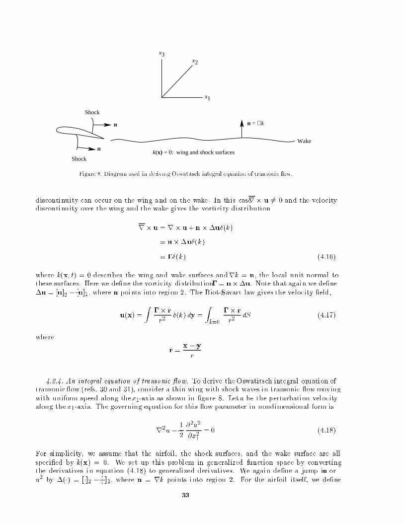
n = ∇k

x3x2

x1

n

Shock

n

Shock

Wake

k(x) = 0: wing and shock surfaces

Figure 8. Diagram used in deriving Oswatitsch integral equation of transonic ow.

discontinuity can occur on the wing and on the wake. In this caser u 6= 0 and the velocitydiscontinuity over the wing and the wake gives the vorticity distribution

r u = r u+ n u(k)

= uu(k)

= (k) (4:16)

where k(x; t) = 0 describes the wing and wake surfaces andrk = n, the local unit normal tothese surfaces. Here we dene the vorticity distribution = nu. Note that again we dene

u = [u]2 [u]1, where n points into region 2. The Biot-Savart law gives the velocity eld,

u(x) =

Z r

r2(k) dy =

Zk=0

r

r2dS (4:17)

where

r =x y

r

4.2.4. An integral equation of transonic ow. To derive the Oswatitsch integral equation oftransonic ow (refs. 30 and 31), consider a thin wing with shock waves in transonic ow moving

with uniform speed along thex1-axis as shown in gure 8. Letu be the perturbation velocityalong the x1-axis. The governing equation for this ow parameter in nondimensional form is

r2u 1

2

@2u2

@x21= 0 (4:18)

For simplicity, we assume that the airfoil, the shock surfaces, and the wake surface are all

specied by k(x) = 0. We set up this problem in generalized function space by convertingthe derivatives in equation (4.18) to generalized derivatives. We again dene a jump inu or

u2 by () = [ ]2 [ ]1, where n = rk points into region 2. For the airfoil itself, we dene

33

[u]1 =u21= 0 because the airfoil is a closed surface. Thus,

r

2u

1

2

@2u2

@x21=

@u

@n

@

@n1

u2

2

(k)

+ r

un

u2

2n1

(k)

(4:19)

where n = (n1; n2; n3) is the unit normal to the surface k = 0 and n1 = (n1; 0; 0). Note thaton the right side of equation (4.19) we dropped the sum of two terms, which by equation (4.18)

is 0.

To get an integral equation, we use the Green's function of the Laplace equation, which is1=4r , and treat @2u2=@x21 as a source term to obtain

4u(x) =

1

2

@2

@x21

Z1

ru2(y) dy

Zk=0

1

r

@u

@n

@

@n1

u2

2

dS

r

Zk=0

1

r

un

u2

2n1

dS (4:20)

Now if we bring the derivatives inside the rst volume integral, which is over the unbounded

space, we must use the nite part of the divergent integral introduced in section 3.4, equa-tion (3.119). Taking Q(y) = u2(y) in equation (3.119), from equation (3.131) we have

@2

@x21

Z1

ru2(y)dy = fu

2(x) + lim"!0

Z3r21 r2

r5h"(y)u

2(y) dy (4:21)

The last integral in equation (4.20) is

r

Zk=0

1

r

un

u2

2n1

dS =

Zk=0

1

r2

u cos

u2

2n1 cos 1

dS (4:22)

where cos = r n, cos 1 = 1=n1 r n1, and r = (x1 y1)=r. Our job is nished. The integralon the right side is convergent. Substitute equations (4.21) and (4.22) in equation (4.20). The

result is the Oswatitsch integral equation of transonic ow. Further approximation is possible,but we stop at this point. This derivation is much shorter and more direct than the original one.

(See refs. 30 and 31.)

4.3. Aeroacoustic Applications

In this section, we give four examples for the linearwave equation. Even for this equation, the

use of generalized function theory leads to important and useful results. Before the examples,we give some standard forms of the inhomogeneous source terms appearing in aeroacoustic

problems. These follow:

2 = Q(x; t) (4 :23a)

2 = Q(x; t)(f ) (4:23b)

34

2 =

@

@t[Q(x; t)(f)] (4:23c)

2 = r [Q(x; t)(f)] (4:23d)

2 = Q

~(x; t)h

~f 0(f ) (4:23e)

2 = Q(x; t)(f )

~f

(4:23f)

In these equations, f(x; t) = 0 is a moving surface, usually assumed a closed surface. Anopen surface, such as a panel on a rotor blade, is described by f = 0 and ~f(x ; t) > 0, wheref(x; t) = ~f(x; t) = 0 describes the edge of the open surface. (See g. 9.) Also, we denote the

Heaviside function as h~f. In equation (4.23e), note that Q

~is the restriction of Q to f = 0.

The solutions of the above equations have been given in many publications of the author and

coworkers. (See refs. 3336.) We give only a brief summary here.

The Green's function of the wave equation is

G(y; ; x; t) =

((g)4r ( t)

0 ( > t)(4:24)

where

g = t +r

c(4:25)

In this equation, (x; t) and (y ; ) are the observer and the eld (source) space-time variables,

respectively. The speed of sound is denoted by c and r = jx yj . The two forms of the solution

n

∇f = n

∇f = ν~

f = f = 0 edge~

f = 0, f > 0~

f = f = 0~

f = 0

f = 0~

f = 0

f > 0~

Figure 9. Denition of open surface by relations f = 0, ~f > 0. Edge is dened by f = ~f = 0 and is the unit inward

geodesic normal.

35

of equation (4.23a) are

4(x; t) =

Z1

r[Q]ret dy (4:26)

and

4(x ; t) =

Z t

1

d

t

Z()

Q(y; )d (4:27)

where the subscript ret stands for retarded time t r=c. The surface ( ) is the spherer = c(t ) (i.e. , the sphere with center at the observer x and radius c(t ) with the elementof the surface denoted by d). The two forms of the solution of equation (4.23a) are known as

the retarded time and the collapsing sphere forms of the solution, respectively.

The solution of equation (4.23b) can also be written in several forms. (See refs. 33 and 34.)We give two forms here. For a rigid surface f(x; t) = 0, let Mr = M r be the local Mach number

in the radiation direction. Then

4(x ; t) =

Zf=0

Q(y ; )

r j1 Mr j

ret

dS (4:28)

Note that to get this equation, the formal Green's function solution, which is

4(x; t) =

Z1

rQ(y; )(f)(g) dy d (4:29)

is integrated as follows. First introduce a Lagrangian variable on and near the surface f = 0such that the Jacobian of the transformation is unity. Note that we have y = y( ; ) and

r = jx y(; )j (4:30)

Next let ! g, which gives @g=@ = 1Mr . Integrate equation (4.29) next with respect to g

and nally integrate (f) by the method of section 3.3 to get equation (4.28).

A more interesting method of integrating the delta functions in equation (4.29) is to let ! g

and integrate with respect to g . The integration gives

4(x; t) =

Z1

r[Q(y; )]ret(F) dy (4:31)

where F (y;x ; t) = [f (y ; )]ret = f [y ; t r=c ]. Note, however, that even if jrf j = 1 bydenition, we have jrF j 6= 1 in equation (4.31). We will, therefore, give a slight modication of

equation (3.80). In the following integral, assume jrf j 6= 1, then

I =

Z(x)(f )dx =

Zf=0

(x)

jrf jdS (4:32)

This result applies to equation (4.31). It is easily shown by dierentiation that

jrF j =1 +M2

n 2Mn cos 12 (4:33)

where Mn = vn=c , vn = @f=@t is the local normal velocity on f = 0, and cos = n r is thecosine of the angle between the local normal to f = 0 and the radiation direction r = (x y)=r.

Using equations (4.32) and (4.33) in equation (4.31), we get

4(x; t) =

ZF=0

1

r

Q(y ; )

ret

d (4:34)

36

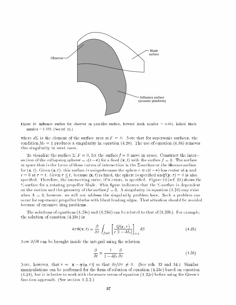
Influence surface (acoustic planform)

Observer

Blade surface

Figure 10. In uence surface for observer on propeller surface, forward Mach number = 0.334, helical Mach

number = 0.880. (See ref. 44.)

where d is the element of the surface area atF = 0. Note that for supersonic surfaces, the

conditionMr = 1 produces a singularity in equation (4.28). The use of equation (4.34) removesthis singularity in most cases.

To visualize the surface : F = 0, let the surface f = 0 move in space. Construct the inter-section of the collapsing spherer = c(t ) for a xed (x; t) with the surface f = 0. The surfacein space that is the locus of these curves of intersection is the -surface or the in uence surface

for (x; t). Given (x; t), this surface is uniquebecause the sphere r = c(t ) has center at x andr = 0 at = t. Given t, because (x; t) is xed, the sphere is specied andf(y; ) = 0 is alsospecied. Therefore, the intersecting curve, if it exists, is specied. Figure 10 (ref. 32) shows the

-surface for a rotating propeller blade. This gure indicates that the -surface is dependenton the motion and the geometry of the surface f = 0. A singularity in equation (4.34) may exist

when = 0; however, we will not address the singularity problem here. Such a problem canoccur for supersonic propeller blades with blunt leading edges. That situation should be avoidedbecause of excessive drag problems.

The solutions of equations (4.23c) and (4.23d) can be related to that of (4.23b). For example,the solution of equation (4.23c) is

4(x; t) =@

@ t

Zf=0

Q(y ; )

r j1 Mr j

ret

dS (4:35)

Now @=@t can be brought inside the integral using the relation

@

@t=

1

1 Mr

@

@(4:36)

Note, however, that r = jx y( ; )j so that @r=@ 6= 0. (See refs. 33 and 34.) Similar

manipulations can be performed for the form of solution of equation (4.23c) based on equation(4.34), but it is better to work with the source terms of equation (4.23c) before using the Green's

function approach. (See section 4.3.3.)

37

The solution of equation (4.23e) is by far the most dicult of the problems considered here.We rst simplify the algebraic manipulations by dening ~f such that r~f = where is the

unit outward geodesic normal to the edge. The geodesic normal is tangent to the surface f = 0,~f > 0 and is orthogonal to edge f = ~f = 0. (See g. 9.) The formal solution of equation (4.23e)

is

4(x ; t) =

Z1

rQ~(y ; )h(~f ) 0(f)(g) dy d

=

Z1

r[Q~(y; )]reth(eF) 0(F) dy (4:37)

where, as before, F = [f ]ret and we dene eF(y; x; t) = [~f(y ; )]ret. Let N be the unit normal to

the surface F = 0. We can show that

N =nMnr

(4:38)

Equation (4.37) is now of the form of equation (3.81). Again, because jrF j = 6= 1, we must

give the modication to equation (3.81) here. In this case, we have for jrf j 6= 1

Z(x) 0(f) dy =

Zf=0

1

jrf j

@

@n

jrf j

+

2Hf

jrf j2

dS (4:39)

Next, using F in place of f here, we get from equation (4.39)

4(x; t) =

ZF=0

8><>:

1

@

@N

0@ [Q

~]ret

rh(eF)

1A +

2HF [Q~]reth(eF )

r2

9>=>; d (4:40)

where HF is the local mean curvature of the -surface given by F = 0. Note that

@

@Nh(eF ) = N reF (eF) (4:41)

so that we must integrate this delta function in equation (4.40). Using a curvil inear coordinatesystem on the -surface, we can show that

ZF=0

(x)jr eF j(eF) d =

ZF=0eF=0

sin0dL (4:42)

where 0 is the angle between N and eN = reF=jreF j. Also, dL is the element of length of the

edge of the -surface given by F = eF = 0. The nal result of manipulations of equation (4.40)based on equation (4.42) is

4(x; t) =

ZF=0eF>0

8<:

1

@

@N

0@ [Q

~]ret

r

1A+

2HF [Q~]ret

r2

9=; d

ZF=0eF=0

[Q~]retcot

0

r2dL (4:43)

38

Note that we have dened eN as the unit normal to eF = 0 and we have

eN = M re (4 :44a)

e = jreF j (4:44b)

cos0 = N eN (4:44c)

Because Q~is the restriction of Q to f = 0, we have @Q

~=@n = 0. In equation (4.43), we nd the

normal derivative of [Q~]ret rst:

@

@N[Q~]ret =

24 @Q

~@N

35ret

+1

c

24 @Q

~@

N r

35ret

(4:45)

Using equation (4.38), we get

N =1

[(1 Mn cos )nMn sint1] (4:46)

where t1 is the unit vector along the projection of r on the local tangent plane to f = 0.Therefore, after using @Q

~=@n = 0 we get

@Q~

@N=

Mn sin

@Q~

@t1(4:47)

where @=@ t1 is the directional derivative ofQ~along t1. In this case, we no longer need restriction

of Q to f = 0 because @Q~=@t1 = @Q=@t1. For @Q

~=@ in equation (4.45), we must use a relation

similar to that in equation (4.10). The curve F = eF = 0 in equation (4.43) is generated by theintersection of the collapsing sphere g = 0 and the edge curve f = ~f = 0 of the open surface

f = 0; ~f > 0.

We next consider equation (4.23f). The formal solution is

4(x ; t) =

Z1

rQ(y; )(f )(~f)(g)dy d

=

Z1

r[Q]ret(F)(eF) dy (4:48)

This equation is similar to equation (3.99) except that jrF j 6= 1 and jr eF j 6= 1. In this

case, sin in equation (3.100) is replaced by jrF reF j , which by denition is 0. Therefore,equation (4.48) gives

4(x; t) =

ZF=0eF=0

1

r

Q

0

ret

dL (4:49)

We now give four applications.

4.3.1. Lowson's formula for a dipole in motion. A dipole is an idealization of a point force.

A point force in motion is described by the wave equation

2p0 =

@

@xiffi(t) [x s(t)]g (4:50)

39

where p0 is the acoustic pressure, fi is the component of the point force, and s(t) is the positionof the force at time t . The formal solution of equation (4.50) is

4p0(x ; t) = @

@xi

Zfi( )

r [y s( )](g) dy d (4:51)

Let us integrate the above integral with respect to y . We get

4p0(x; t) = @

@xi

Zfi( )

r(g) d (4:52)

where

r = jx s()j (4 :53a)

and

g = t +r

c(4:53b)

Now let ! g and note that@g

@ = 1 Mr (4:54)

where Mr = _s r=c is the Mach number of the point force in the radiation direction. Integrate

the resulting equation with respect to g to get

4p 0(x; t) = @

@xi

fi( )

r j1 Mr j

(4:55)

where is the emission time. The solution of g = 0 has only one root if the point force is insubsonic motion. The derivative in equation (4.55) can now be taken inside the square brackets.

The resulting equation is a formula given by Lowson (ref. 37) that is useful in noise predictionof rotating blades where the dipole sources can by assumed compact.

4.3.2. Kirchho formula for moving surfaces. In the 1930's, Morgans published a paper inwhich he derived the Kirchho formula for moving surfaces. (See ref. 38.) The derivation of this

formula was based on classical analysis and was lengthy. In 1988, Farassat and Myers gave amodern derivation of this result based on generalized function theory. (See refs. 39 and 40.) The

derivation is short and avoids the use of four-dimensional Green's identity and the associateddiculties of dealing with surfaces and volumes in four dimensions. We present the basic ideabehind this modern derivation here and refer the readers to reference 39.

Assume that the surface in motion on which conditions on (x; t) are specied is given byf(x; t). This surface can be deformable. Assume that satises the wave equation in the

exterior of the surface f = 0, which is the region dened by f > 0. Now extend to the entireunbounded space as follows:

~(x; t) =

((x; t) (f > 0)

0 (f < 0)(4:56)

Clearly, ~ satises the wave equation in the unbounded space. However, ~ has discontinuities

across f = 0 that appear as source terms of the wave equation. Note that the jumps in~ and its derivatives depend on corresponding values for because ~ = (f = 0+) and

@ ~=@ t = @=@t (f = 0+).

40

Applying the rules of generalized dierentiation to ~ , we get

2~ = n +

1

cMnt

(f) 1

c

@

@t[Mn(f)] r [n(f)] (4:57)

where Mn = vn=c and vn = @f=@t is the local normal velocity of the surface f = 0. As before,we have assumed rf = n, the local outward unit normal to f = 0. The three types of source

terms on the right of equation (4.57) are of the standard types given in equations (4.23af). Thesolution for a deformable surface is given by

4~(x; t) =

ZD(S)

E1

pg(2)

r (1 Mr)

du1 du2 +

ZD(S)

E2

pg(2)

r (1Mr)

du1 du2 (4:58)

where D(S) is a time-independent region in u1u2-space onto which the surface f = 0 is mapped.The determinant of the coecient of the rst fundamental form is denoted g(2). In this equation

is the emission time of the pointu1 ; u2

on the surface f = 0. The expression E1 depends on

, n , r2 (surface gradient of ), and the kinematic and geometric parameters of the surface

f = 0. The expression E2 depends only on the kinematic and geometric parameters of thesurface f = 0. (See ref. 39.)

4.3.3. Noise from moving surfaces. Let an impenetrable surface f = 0 be in motion such

that f > 0 outside the body and rf = n, the unit outward normal. Let us assume that the uid is extended inside this surface with conditions of undisturbed medium (i.e., density 0 and

speed of sound c). We know that the mass continuity and momentum equations are valid whenthe derivatives are written as generalized derivatives. Let us extract only the contribution ofdiscontinuities across f = 0 and leave the eect of all other discontinuities (such as those across

shock waves) in these equations. The mass continuity equation gives

@

@t+r (u) = ( 0)vn(f) + un(f)

= 0vn(f) (4:59)

where n = @f=@t is the local normal velocity of f = 0 and we have used the impenetrabilitycondition on this surface, which is un = n . The momentum equation gives

@

@t(ui) +

@

@xj

uiuj +Pij

=Pij nj(f) (4:60)

where Pij = E ij + (p p0)ij is the compressive stress tensor and Eij is the viscous stress

tensor. Now we take the generalized derivative of both sides of equation (4.59) and @=@xi of

both sides of equation (4.60), subtract the latter from the former, and nally subtract c2 @2=@x2i

from both sides to get

2p0 = @

2

@xi @xj

Tijh(f)

@

@xi

Pij nj(f)

+

@

@t[0vn(f)] (4:61)

where p0 = c2( 0). Here Tij is the Lighthill stress tensor. Now we have added h(f), the

Heaviside function, on the right side to indicate that Tij 6= 0 outside the surface f = 0. This isthe Ffowcs Will iamsHawkings (FW-H) equation. (See ref. 41.) Note that in the far eld, p0 isthe acoustic pressure.

41

The source terms of equation (4.61) are of the standard types in equations (4.23af). Fora surface in subsonic motion, the solution for surface sources involving the Doppler factor is

most appropriate for numerical work. (See refs. 33 and 34.) For supersonic surfaces such asan advanced propeller blade on which jMnj < 1 everywhere, a dierent solution based on the

-surface must be used. We show here brie y how this can be done. In applications, we need tocalculate the sound from an open surface such as a panel on a blade. We, therefore, dene suchan open surface by f = 0; ~f > 0 with the edge dened by f = ~f = 0 as before. The assumptions

concerning the gradients of f and ~f at the beginning of this section hold here. We are interestedin the solution of equations of the types

2p0 =

@

@t

h0vnh(~f)(f)

i(4 :62a)

2p0 =

@

@xi

hpnih(~f)(f)

i(4:62b)

where h(~f) is the Heaviside function. Note that we have approximatedPij in equation (4.61) bypij where p is the surface (gauge) pressure. To derive solutions for equations (4.62a)and (4.62b)

suitable for supersonic panel motion, we write

@

@t

0vn~h(~f)(f)

= 0

@vn~

@th(~f)(f)

0vn~

2h(~f ) 0(f)

0 vn v(~f)(f) (4:63)

where v is the velocity of the edge in the direction of the geodesic normal. A similar operation

can be performed on the right of equation (4.62b) such that

@

@xi

hpnih(

~f )(f)i= r

p~nh(~f)(f )

= p~h(~f) 0(f)+ 2pHfh(

~f)(f ) (4:64)

where Hf is the local mean curvature of the surface f = 0. The source terms of the right of

equations (4.63) and (4.64) are of the types in equations (4.23af). (See refs. 35 and 36.)

4.3.4. Identication of shock noise source strength. The rst term on the right of theFW-H equation (4.61) is known as the quadrupole source. As mentioned in the derivations,

the discontinuities in the region f > 0 (i.e. , outside the body) contribute source terms aftergeneralized dierentiation is performed. If a shock wave described by the equation k(x ; t) = 0

exists on a rotating blade, then the quadrupole term gives surface sources on the shock, the

42

strengths of which are determined as follows. Let us take the generalized second derivative ofTij by

@Tij

@xi

=@Tij

@ xi

+ Tijn0

i(k) (4:64a)

@2Tij

@xi @xj

=@2Tij

@xi @xj

+ @Tij

@xi

n 0j(k) +@

@xj

Tijn

0

i(k)

(4:65b)

where n0 = rk is the unit normal to the shock surface pointing to the downstream region. The

last two terms on the right of this equation are shock surface terms that are of monopole anddipole types, respectively. The rst term on the right of equation (4.65b) is a volume term thatis familiar in Lighthill 's jet noise theory. In the rotating blade noise problem, this term primarily

re ects nonlinearities other than turbulence. Farassat and Tadghighi (ref. 42) conjectured thatthe shock surface terms contributed relatively more than the volume term in equation (4.65b).

Preliminary calculations have supported this conjecture. (See ref. 43.)

The interesting aspect in the above result is that the shock source strength is obtainedpurely by mathematics. Without the use of the operational properties of generalized functions,the identication of shocks as sources of sound and the determination of the source strength

would be rather dicult. Other mechanisms of noise generation can also be identied by thismethod. (See ref. 44.)

5. Concluding Remarks

In this paper, we have given the rudiments of generalized function theory and someapplications in aerodynamics and aeroacoustics. These applications depend on the conceptof generalized dierentiation and on the Green's function approach. We have brie y discussed

the generalized Fourier transformation. Many more examples could be given. The power ofthis theory stems from its operational properties. In addition to the exchange of limit processes

that leads to many useful results, discontinuous solutions of linear equations using the Green'sfunction are easily obtained by posing the problem in generalized function space. As seen in theexample of the Oswatitsch integral equation of transonic ow, a nonlinear partial dierential

equation with a discontinuous solution can be cast into an integral equation based on thefundamental solution of the linear part of the dierential equation. The Schwartz generalized

function theory has unied many ad hoc methods in mathematics and has answered somefundamental questions about linear partial dierential equations. The nonlinear theory nowbeing developed, in which multiplication of generalized functions is allowed, can be even more

useful in applications. Generalized function theory is an extension of classical analysis and givesengineers and scientists added power in applications. This extension is much like the complexanalysis that extends real analysis and is very important in applied mathematics. Finally,

multidimensional generalized functions, particularly the delta function and its derivatives, arequite useful in many applications.

NASA Langley Research Center

Hampton, VA 23681-0001

January 28, 1994

43

References

1. Schwartz, L.: Theories des Distributions, Volumes I and II. Actualities Scientiques et Industrielles, Hermann andCie (Paris, France), 1957.

2. Jones, D. S.: The Theory of Generalised Functions. Second ed., Cambridge Univ. Press, 1982.

3. Stakgold, Ivar: Boundary Value Problems of Mathematical Physics, Volume II. The MacMillan Co., 1968.

4. Kanwal, Ram P.: Generalized Functions|Theory and Technique. Academic Press, 1983.

5. De Jager, E. M.: Applications of Distributions in Mathematical Physics. 2nd ed., Mathematisch Centrum(Amsterdam), 1969.

6. Lighthill, M. J.: Introduction to Fourier Analysis and Generalized Functions. Cambridge Univ. Press, 1964.

7. Gel'fand, I. M.; and Shilov, G. E. (Eugene Saletan, Transl.): Generalized Functions. Volume 1|Properties and

Operations. Academic Press, 1964.

8. Aris, Rutherford: Vectors, Tensors, and the Basic Equations of Fluid Mechanics. Dover Publ. Inc., 1989.

9. McConnell, A. J.: Applications of Tensor Analysis. Dover Publ., Inc., 1957.

10. Carmichael, Richard D.; and Mitrovic, Dragisa: Distributions and Analytic Functions. John Wiley & Sons, Inc.,1989.

11. Robertson, A. P.; and Robertson, Wendy: Topological Vector Spaces. Cambridge Univ. Press, 1964.

12. Bremermann, H. J.; andDurand, L., III: On Analytic Continuation,Multiplication, and Fourier Transformationsof Schwartz Distributions. J. Mathematical Physics, vol. 2, no. 2, Mar.Apr. 1961, pp. 240258.

13. Bremermann, Hans: Distributions, Complex Variables, and Fourier Transforms. Addison-Wesley Publ. Co., Inc.,1965.

14. Synowiec, John: Distributions: The Evolution of a Mathematical Theory. Historia Mathematica, vol. 10, 1983,pp. 149183.

15. Lutzen, Jesper: The Prehistory of the Theory of Distributions. Springer-Verlag, 1982.

16. Dieudonne, Jean: History of Functional Analysis . Elsevier Sci. Publ. Co., Inc., 1981.

17. Antosik, Piotr; Mikusinski, Jan; and Sikorski, Roman: Theory of Distributions|The Sequential Approach.Elsevier Sci. Publ. Co., 1973.

18. Mikusinski, Jan: Operational Calculus|Volume I. Second ed., PergamonPress, Inc., 1983.

19. Mikusinski, Jan; and Boehme, Thomas K.: Operational Calculus|Volume II. Second ed., Pergamon Press Inc.,1983.

20. Erdelyi, Arthur: Operational Calculus and Generalized Functions. Holt, Rinehart and Winston, Inc., 1962.

21. Robinson, Abraham: Non-Standard Analysis. North-Holland Publ. Co., 1966.

22. Colombeau, Jean Francois: New Generalized Functions and Multiplication of Distributions. Elsevier Sci. Publ.Co., Inc., 1984.

23. Colombeau, JeanFrancois: Elementary Introduction to New Generalized Functions. Elsevier Sci. Publ. Co., Inc.,1985.

24. Rosinger, Elemer E.: Non-Linear Partial Dierential Equations|An Algebraic View of Generalized Solutions.Elsevier Sci. Publ. Co., Inc., 1990.

25. Oberguggenberger, M.: Multiplication of Distributions and Applications to Partial Dierential Equations.John Wiley & Sons, Inc., 1992.

26. Rosinger, Elemer E.: Generalized Solutions of Nonlinear Partial Dierential Equations. Elsevier Sci. Publ. Co.,

Inc., 1987.

27. Colombeau, Jean Francois: Multiplication of Distributions. Springer-Verlag, 1992.

28. Zemanian, A. H.: DistributionTheory and Transform Analysis|An Introduction to Generalized Functions, With

Applications. Dover Publ. Inc., 1987.

44

29. Richards, Ian; and Youn, Heekyung: Theory of Distributions: A Non-Technical Introduction. Cambridge Univ.

Press, 1990.

30. Oswatitsch, K.: Die Geschwindigkeitsverteilung bei lokalen Uberschallgebieten an achen Prolen. Z. Angew.

Math. Mech., Bd. 30, Nr. 1/2, Jan.Feb. 1950, pp. 1724.

31. Spreiter, John R.; and Alksne, Alberta: Theoretical Prediction of Pressure Distributions on Nonlifting Airfoils

at High Subsonic Speeds. NACA Rep. 1217, 1955. (Supersedes NACA TN 3096.)

32. Dunn,Mark H.: The Solutionof a Singular Integral EquationArising From a LiftingSurface Theory for Rotating

Blades. Ph.D. Dissertation from the Department of Computational and Applied Mathematics, Old Dominion

Univ., Aug. 1991.

33. Farassat, F.: Linear Acoustic Formulas for Calculation of Rotating Blade Noise. AIAA J., vol. 19, no. 9,

Sept. 1981, pp. 11221130.

34. Brentner, KennethS.: Prediction of Helicopter Rotor Discrete Frequency Noise|A Computer Program Incorpo-

rating Realistic Blade Motions and Advanced Acoustic Formulation. NASA TM-87721, 1986.

35. Farassat,F.; andMyers, M.K.: The MovingBoundary Problem for the Wave Equation: Theory andApplication.

Computational Acoustics|Algorithms and Applications, Volume 2. Ding Lee, Robert L. Sternberg, and

Martin H. Schultz, eds., Elsevier Sci. Publ. B.V., 1988, pp. 2144.

36. Farassat, F.; and Myers, M. K.: Aeroacoustics of High Speed Rotating Blades: The Mathematical Aspect.

Computational Acoustics|AcousticPropagation,Volume 2,Ding Lee, Robert Vichnevetsky, and AllenRobinson,

eds., Elsevier Sci. Publ. B.V., 1993, pp. 117148.

37. Lowson, M. V.: The Sound Field for Singularities in Motion. Proc. R. Soc. London, ser. A, vol. 286, no. 1407,

Aug. 1965, pp. 559572.

38. Morgans, W. R.: The Kirchho Formula Extended to a Moving Surface. Philos. Mag., vol. 9, 1930, pp. 141161.

39. Farassat, F.; and Myers, M. K.: Extension of Kirchho's Formula to RadiationFrom Moving Surfaces. J. Sound

& Vib., vol. 123, no. 3, 1988, pp. 451460.

40. Hawkings, D. L.: Comments on \Extensionof Kirchho'sFormula to RadiationFromMovingSurfaces." J. Sound

& Vib., vol. 133, no. 1, 1989, p. 189. Response by F. Farassat andM. K. Myers (same journal and page).

41. Ffowcs Williams, J. E.; and Hawkings, D. L.: SoundGenerationby Turbulence and Surfaces in Arbitrary Motion.

Philos. Trans. R. Soc. London, ser. A, vol. 264, no. 1151, May 8, 1969, pp. 321342.

42. Farassat, F.; and Tadghighi, H.: Can Shock Waves on Helicopter Rotors Generate Noise? A Study of the

Quadrupole Source. 46th Annual Forum Proceedings, American Helicopter Soc., vol. 1, 1990, pp. 323346.

43. Tadghighi, H.; Holz, R.; Farassat, F.; and Lee, Yung-Jang: Development of a Shock Noise Prediction Code for

High-SpeedHelicopters|The Subsonically Moving Shock. 47th Annual Forum Proceedings, AmericanHelicopter

Soc., vol. 2, 1991, pp. 773790.

44. Farassat, F.; and Myers, M. K.: An Analysis of the Quadrupole Noise Source of High Speed Rotating Blades.

ComputationalAcoustics|Scattering,Gaussian Beams, and Aeroacoustics, Volume 2, Ding Lee, Ahmet Cakmak,

and Robert Vichnevetsky, eds., Elsevier Sci. Publ. Co., Inc., 1990, pp. 227240.

45

REPORT DOCUMENTATION PAGEForm Approved

OMB No. 0704-0188

Public r eporting burden for this co llection of information is estimated to a vera ge 1 hour per response, including the time for reviewing instr uctions, sear ching ex isting data source s,g ather ing and maintaining the data needed, and completing and reviewing the co llection o f inf ormation. Send comments r egar ding this burden estimate or any o ther a spect of thisco llection of inf ormation, including sugg estions for r educing this burden, to Washington Headquar ter s Se rvices, Dir ectora te fo r Information Operations and Repo rts, 1 21 5 J eersonDav is Highway, Suite 12 04 , Arlington, VA 222 02 -4 30 2, and to the Oce o f Mana gement and Budg et, Paperwork Reduction Pr oject (07 04 -0 18 8), Washing ton, DC 2 05 03 .

1. AGENCY USE ONLY(Leave b lank) 2. REPORT DATE 3. REPORT TYPE AND DATES COVERED

May 1994 Technical Paper

4. TITLE AND SUBTITLE

Introduction to Generalized Functions With Applications

in Aerodynamics and Aeroacoustics

6. AUTHOR(S)

F. Farassat

7. PERFORMING ORGANIZATION NAME(S) AND ADDRESS(ES)

NASA Langley Research CenterHampton, VA 23681-0001

9. SPONSORING/MONITORING AGENCY NAME(S) AND ADDRESS(ES)

National Aeronautics and Space Administration

Washington, DC 20546-0001

5 . FUNDING NUMBERS

WU 535-03-11-02

8 . PERFORMING ORGANIZATION

REPORT NUMBER

L-17300

10. SPONSORING/MONITORING

AGENCY REPORT NUMBER

NASA TP-3428

11 . SUPPLEMENTARY NOTES

Corrected for misprints April 3, 1996

12a. DISTRIBUTION/AVAILABILITY STATEMENT 12b . DISTRIBUTION CODE

UnclassiedUnlimited

Subject Category 71

13 . ABSTRACT (Maximum 200 words)

Generalized functions have many applications in science and engineering. One useful aspect is that dis-

continuous functions can be handled as easily as continuous or dierentiable functions and provide a powerful

tool in formulating and solving many problems of aerodynamics and acoustics. Furthermore, generalized

function theory elucidates and unies many ad hoc mathematical approaches used by engineers and scientists.

Wedene generalized functions as continuous linear functionals on the space of innitelydierentiable functions

with compact support, then introduce the concept of generalized dierentiation. Generalized dierentiation

is the most important concept in generalized function theory and the applications we present utilize mainly

this concept. First, some results of classical analysis, are derived with the generalized function theory. Otherapplications of the generalized function theory in aerodynamics discussed here are the derivations of general

transport theorems for deriving governing equations of uid mechanics, the interpretation of the nite part of

divergent integrals, the derivation of the Oswatitsch integral equation of transonic ow, and the analysis of

velocity eld discontinuities as sources of vorticity. Applications in aeroacoustics include the derivation of the

Kirchho formula for moving surfaces, the noise from moving surfaces, and shock noise source strength based

on the Ffowcs WilliamsHawkings equation.

14 . SUBJECT TERMS 15. NUMBER OF PAGES

Generalized functions; Green's function; Aerodynamics; Aeroacoustics; Wave

equation; Rotating blade noise; Ffowcs WilliamsHawkings equation52

16. PRICE CODE

A04

17 . SECURITY CLASSIFICATION 18. SECURITY CLASSIFICATION 19 . SECURITY CLASSIFICATION 20. LIMITATION

OF REPORT OF THIS PAGE OF ABSTRACT OF ABSTRACT

Unclassied Unclassied

NSN 7540-01-280-5500 Standard Form 298(Rev. 2-89)Pre scr ibed by ANSI Std. Z39-1 82 98 -1 02