introduction to earth system modeling framework (esmf): an...
TRANSCRIPT

Introduction to Earth System Modeling Framework (ESMF): An Atmosphere-Ocean
Modeling Application Example������
Ufuk Turuncoglu (1,2)������������
(1) Informatics Institute, ���Computational Science and Engineering, ���
ITU, Turkey���(2) ESP Section, ���
ICTP, Italy
Dev
elop
er S
choo
l for
HPC
app
licat
ions
in E
arth
Sci
ence
s, 10
-12
Nov
. 201
4
Earth System Modeling Framework (ESMF)
• Complete set of Fortran interface and some C/C++ interfaces • Open source project:���
http://www.earthsystemmodeling.org���http://sourceforge.net/projects/esmf���http://sourceforge.net/projects/esmfcontrib
• Well documented and support
• Well tested (nightly builds on different OS, Architecture, Compiler and MPI versions) and very portable
• Interpolation capability also available via Python (ESMP) ���and NCL (NCAR Command Language)
• New layer to simplify model coupling: The National Unified Operational Prediction Capability (NUOPC)���https://www.earthsystemcog.org/projects/nuopc/

ESMF Architecture
• There are two main type of classes – Superstructure
• Components (gridded and coupler) + States
– Infrastructure • Data Structures (Array, Field, Grid, Bundle)
• Utilities (Clock, VM, Config etc.)
ESMF “sandwich” ���architecture

Superstructure
• Components – Gridded – describes a user component (atm, ocn, etc.) that takes
one import and one export State. ���In general, the fields within import and export State will use same discrete grid.
– Coupler – it takes one or more import States as input and applies spatial/temporal interpolation and/or extrapolation onto one or more output export States.���In general, import and export States are in different discrete grid.
• Different combination of gridded and coupler components:
COMP
import export

Superstructure
• It also contains methods related with – State
– Web services • States
– It contains the data and metadata to be transferred between ESMF Components.
– There are two types of States, import and export.
– An import State contains data that is necessary for a Gridded Component or Coupler Component to execute,
– and an export State contains the data that a Gridded Component or Coupler Component can make available.
– States can contain Arrays, ArrayBundles, Fields, FieldBundles, and other States (in a specific VM).

Infrastructure
• Fields and Grids – Array and Field are used to store data
– Array contains a data pointer along with information about data type, precision and dimension
– Field holds model and/or observational data with its underlying grid or set of spatial locations
– Bundles are the collections of Arrays (ArrayBundle) or Fields (FieldBundle)
– Grid definition (Grid, Mesh and XGrid)
• Utilities – They are a set of tools for quickly assembling modeling
applications • Attribute, Time Management (+Clock), Config, LogErr, DELayout, ���
VM and I/O Utilities

Parallelization
• Sequential (Consecutive) vs. Concurrent
Sequential
Concurrent
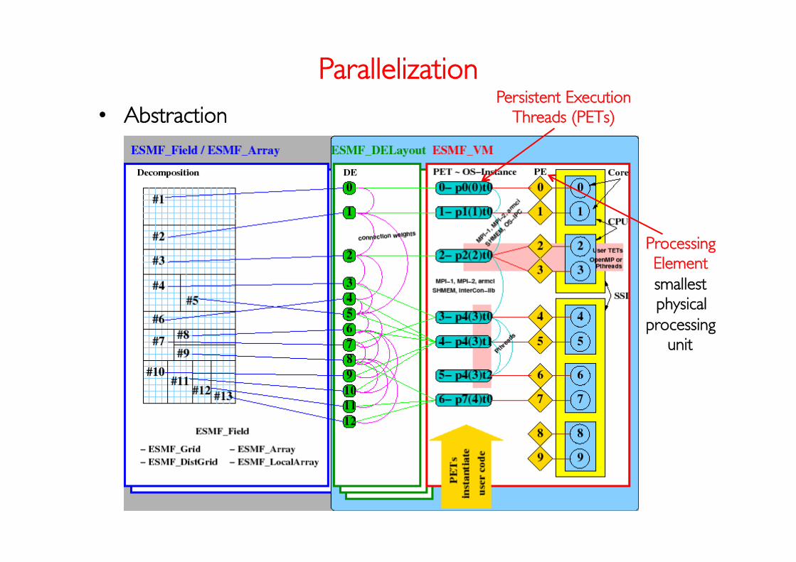
Parallelization
• Abstraction Persistent Execution ���
Threads (PETs)
Processing���Element smallest physical
processing unit
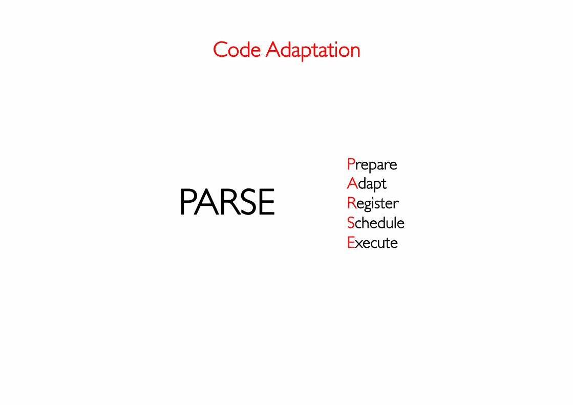
Code Adaptation
PARSE Prepare Adapt Register Schedule Execute

Preparing
1. Prepare user code – Decide on components and model design
– Decide on coupling (or exchange) fields
– Decide on control flow (order of the execution of components) – Split component code into initialize, run and finalize sections

Preparing
• Split model code: initialization, run and finalize (i.e. RegCM)
reads global namelist, read ICBC, ���initialize model and setup output files
run model between given interval get/put routines will retrieve/send data
close files, clean memory and kill processes

Adapting
2. Adapt data structures – Wrap component grid in Grid or Xgrid object
– Wrap data structures in Array and/or Field objects
– Wrap time information in Clock object
ESMF_DistGrid
ESMF_GridCreate
ESMF_GridAddCoord
ESMF_GridAddItem
Retrieve Ptr and Fill
x N (stagger)
x N (mask + area)
defines domain ���decomposition
all coord and item
orde
r
ESMF_FieldCreate
Retrieve Ptr and Fill
Add to State
stagger + type
ESMF_Clock
reference start stop calendar time step

Adapting
• Arrays vs. Fields – Arrays represent user data in index space. They don’t have coordinate
information. So, Arrays can not be used to calculate interpolation weights.
– To do interpolation, user need to supply interpolation weights externally and SMM can be applied to Array.
– Field object includes coordinates. So, it represents user data in physical space.
• Grid Definition – The most important part of the model adaptation.
– Be careful about the definition of halo or ghost regions
– ESMF uses right-hand-coordinate system and smallest stride to the first dimension. The order of dimension can be reversed some times.
– The actual grid definition might be check by ESMF_GridWriteVTK. It creates a set of VTK files (separated for each PET and read by Visit)

Registering
3. Register user methods – Attach user code methods to the framework through
registration calls – Create register routine for each component (gridded or coupler)
– The register routine attaches initialization, run and finalize routines. By this way, ESMF know the routines to control ESMF_[Grid | Cpl]CompSetEntryPoint
– Then register routines called in main application to allow ESMF take control of the model components. ���ESMF_[Grid | Cpl]CompSetServices
• Then, the registered model components can be initialized – Definition of grids – States (import and export)
– Clocks

Scheduling
4. Schedule, synchronize and send the data – The scheduling, synchronization and data exchange can be
controlled via coupler (optional) – In this case, all the data redirected by coupler / driver. There is no
direct interaction among the components. – Regridding, SMM, data redistribution
– Different scheduling options exists • Explicit
• Semi-implicit
• Implicit
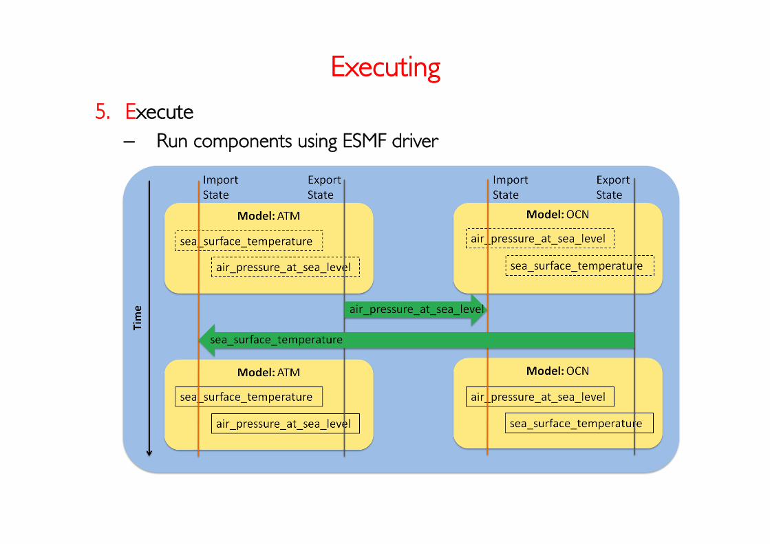
Executing
5. Execute – Run components using ESMF driver

ESMF / NUOPC Layer
• National Unified Operational Prediction Capability – Consortium of U.S. operational weather and water prediction
centers – NOAA, Navy, Air Force, NASA, and other associated modeling
groups – http://earthsystemcog.org/projects/nuopc/
• It is a software layer implemented on top of ESMF
• It defines generic components (Model, Mediator, Connector and Driver). The generic components can be customized by attachable methods.
• It contains utility methods for common tasks
• It contains Field dictionary (standard names and units)
• It is distributed with ESMF
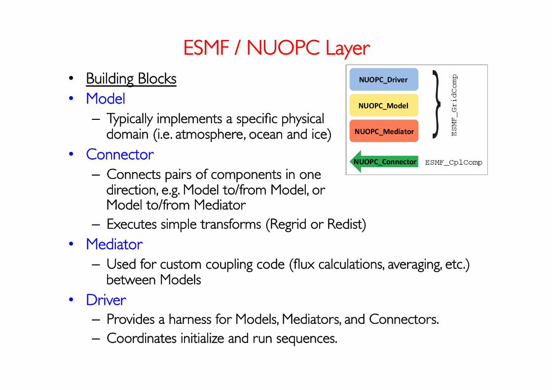
ESMF / NUOPC Layer • Building Blocks • Model
– Typically implements a specific physical ���domain (i.e. atmosphere, ocean and ice)
• Connector – Connects pairs of components in one ���
direction, e.g. Model to/from Model, or ���Model to/from Mediator
– Executes simple transforms (Regrid or Redist) • Mediator
– Used for custom coupling code (flux calculations, averaging, etc.) between Models
• Driver – Provides a harness for Models, Mediators, and Connectors. – Coordinates initialize and run sequences.
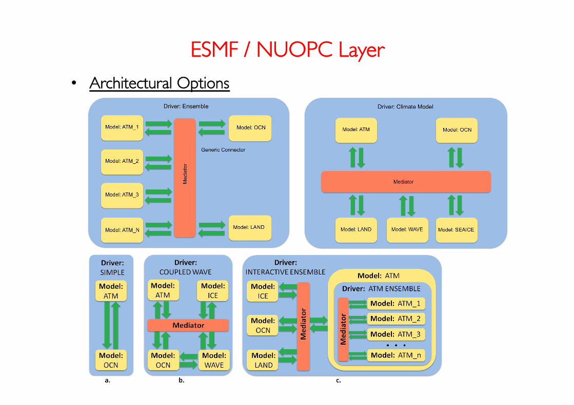
ESMF / NUOPC Layer
• Architectural Options
Test Case
• The code that is used in the test case are extracted from RegESM (Regional Earth System Model)
• The component codes are removed to have a independent, easy to use and understand test code
• It demonstrates: – Creation and running components (gridded + coupler)
– Creating grids via SCRIP formatted netCDF files – Generation of routehandles (online)
• Main component of the regridding and stores weight matrices
• Components need to different routhandle for different grids and interpolation types
– Regridding using routehandles • Two step interpolation to fix land-sea mask mismatch
• Interpolation (bilinear) + Extrapolation (nearest-neighbor)
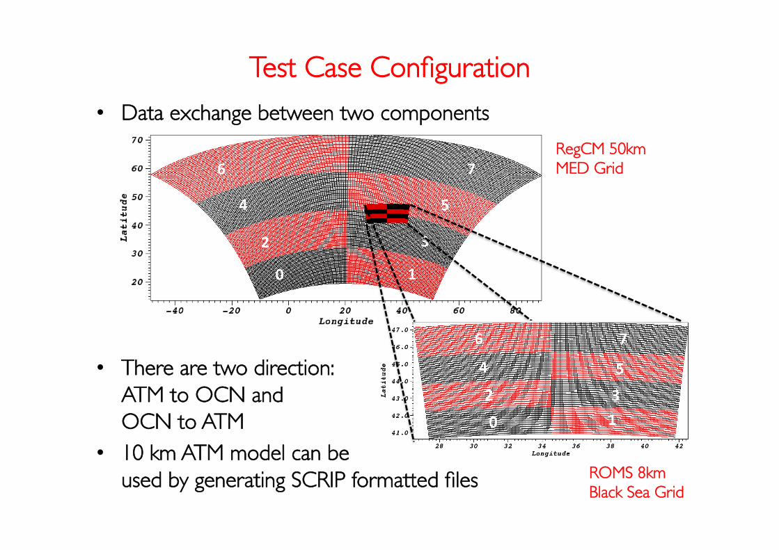
Test Case Configuration
• Data exchange between two components
• There are two direction:���ATM to OCN and ���OCN to ATM
• 10 km ATM model can be���used by generating SCRIP formatted files
0
3
4
7
1
2
5
6
0
4
2
6
1
5
3
7
RegCM 50km ���MED Grid
ROMS 8km ���Black Sea Grid

Exchange Field
• Input field from standard SCRIP tests fields • Pseudo spherical harmonics (L=32, M=16)
• It is good to have a field that has a analytical solution. The interpolation error can be estimated in this case.
http
://oc
eans
11.la
nl.g
ov/t
rac/
SCR
IP
f = 2+ sin16 (2! )cos(16") ! = lat, " = lon
• Regridding is performed���only over sea
• In this case, ATM���component will send���masked data

Description of Test Code
• Get the code
• The list of the files
ESMF_netcdf_read.f
Makefile
fix.sh
main.F90
main.job
namelist.rc
proc
user_coupler.F90
user_model1.F90
user_model2.F90 Gridded components code (model1: ATM, model2: OCN)
Coupler component code (field interpolation) Directory to create SCRIP definition of grids
Reads components grid information (from netCDF) Compiles test case Adds coordinate information to output of the test app Main program (creates components and trigger them)
Job submission script
Configuration file (decomposition, files etc.)
https://www.dropbox.com/s/hwfk4b39bxyovll/smr2613.tar.gz?dl=0

Login and Environment Setup
• Login to Argo cluster • Load required modules
• Still need to define a set of environment variables
module use-append /opt/smr2613/modules/usermodule module purge module load esmf-6.3.0r module load ncl-6.2.1-gcc-4.4.7 module load pnedcdf-1.3.1 module load zlib-1.2.8 module load hdf5-1.8.11-intel module load netcdf-4.3.0 module load xerces-3.1.1
setenv ESMF_LIB "${ESMF_INSTALL_PREFIX}/lib/lib${ESMF_BOPT}/${ESMF_OS}.${ESMF_COMPILER}.${ESMF_ABI}.${ESMF_COMM}.${ESMF_SITE}" setenv ESMFMKFILE "${ESMF_LIB}/esmf.mk" setenv LD_LIBRARY_PATH ${ESMF_LIB}:${LD_LIBRARY_PATH} setenv PATH ${ESMF_INSTALL_PREFIX}/bin/bin${ESMF_BOPT}/${ESMF_OS}.${ESMF_COMPILER}.${ESMF_ABI}.${ESMF_COMM}.${ESMF_SITE}:${PATH}
in csh shell
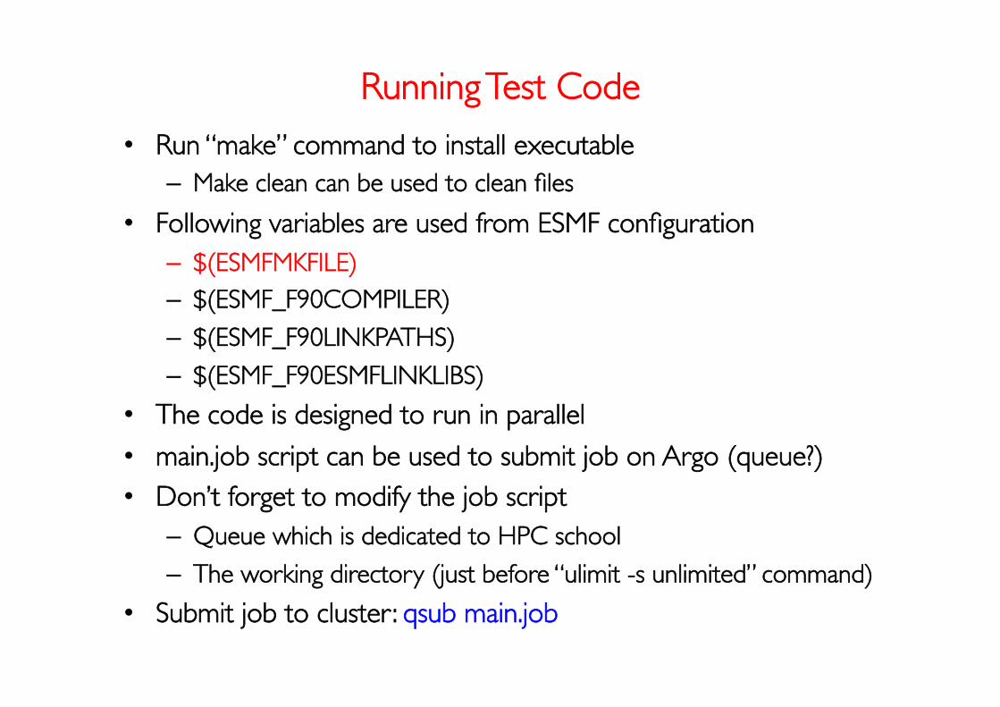
Running Test Code
• Run “make” command to install executable – Make clean can be used to clean files
• Following variables are used from ESMF configuration – $(ESMFMKFILE) – $(ESMF_F90COMPILER)
– $(ESMF_F90LINKPATHS)
– $(ESMF_F90ESMFLINKLIBS)
• The code is designed to run in parallel
• main.job script can be used to submit job on Argo (queue?) • Don’t forget to modify the job script
– Queue which is dedicated to HPC school
– The working directory (just before “ulimit -s unlimited” command)
• Submit job to cluster : qsub main.job

Analyzing Output
• There are four group of files – *.vtk files store information about grid definition for each
component (each PET has its own part) – gcomp*.nc files have initial data stored by components
– remap*.nc files are the fields after interpolation • 1: interpolation,
• 2: interpolation + extrapolation • forward: ATM to OCN
• backward: OCN to ATM
– mask*.nc files store mask information (created by “UTIL_FindUnmapped” subroutine in user_coupler.F90) • 0: land
• 98: mapped grid points (filled just after bilinear interpolation)
• 99: unmapped grid points (needs extrapolation)
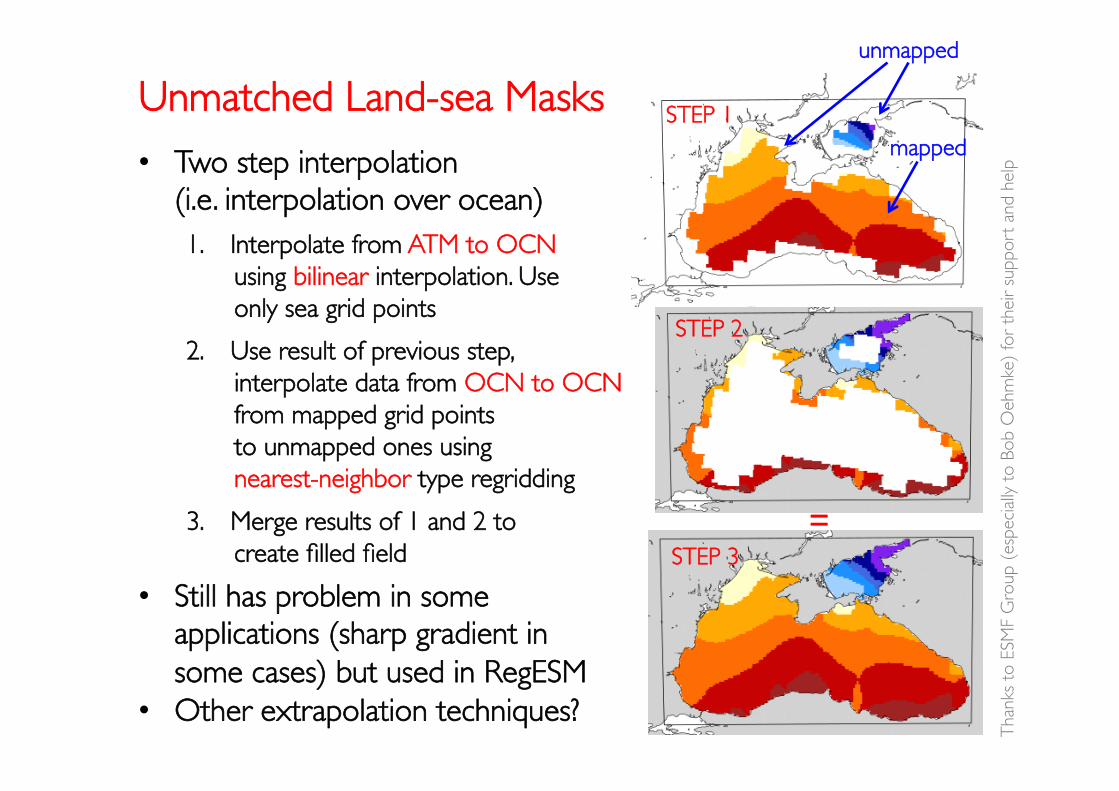
• Two step interpolation ���(i.e. interpolation over ocean)
Unmatched Land-sea Masks
STEP 2 2. Use result of previous step, ���
interpolate data from OCN to OCN ���from mapped grid points ���to unmapped ones using���nearest-neighbor type regridding
3. Merge results of 1 and 2 to���create filled field
+
STEP 3 =
• Still has problem in some applications (sharp gradient in some cases) but used in RegESM
• Other extrapolation techniques?
Tha
nks
to E
SMF
Gro
up (
espe
cial
ly t
o Bo
b O
ehm
ke)
for
thei
r su
ppor
t an
d he
lp
STEP 1
1. Interpolate from ATM to OCN���using bilinear interpolation. Use ���only sea grid points
mapped
unmapped
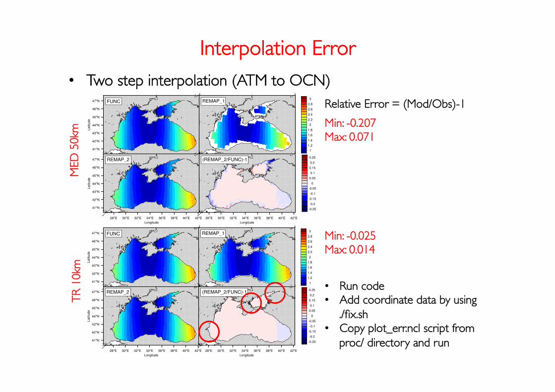
Interpolation Error
• Two step interpolation (ATM to OCN)
Min: -0.207���Max: 0.071
Min: -0.025���Max: 0.014
MED
50k
m
TR
10k
m
Relative Error = (Mod/Obs)-1
• Run code • Add coordinate data by using ���
./fix.sh • Copy plot_err.ncl script from
proc/ directory and run