introduction to depthmap -...
TRANSCRIPT

Introduction to
UCL Depthmap 10
September2010
Version 10.08.00r
Joao Pinelo, Alasdair Turner

Introduction to Depthmap
•Ease-up the first contact with the software
•Understand potential and limitations
•Learn general proceedings
•Cover operational issues which may be less documented
Objectives

Outline
1.Introduction (3)
2.Drawing files (7)
3.Visibility Graph Analysis (14)
4. Convex Map Analysis (27)
5. Axial Map Analysis (37)
6.Segment Map Analysis (44)
7.Data Management/Analysis (50)
8.Agents (57)
9.Conclusion (59)
Introduction to Depthmap
Introduction
Why use Depthmap?
Research findings
What is Depthmap? What it does and doesn’t.
It is a tool for topological analysis
The analysis of layouts is achieved through the
juxtaposition of graphs
The graphs are analysed

A brief summary of Research Findings•Topologically based measures (integration, which is a measure of topological accessibility) correlates significantly with pedestrian and vehicular movement patterns.
•Isovist properties, such as area, correlate with spatial behaviour.
•The representations of layouts (as convex, axial or visibility graphs) and the topological and angular analysis seem to have a correspondence to the way humans cognise space, maybe because they reflect embodiment.
References
Dalton, R. C. 2002, "Is spatial intelligibility critical to the design of large-scale virtual environments?", International Journal of Design Computing, vol. 4.
Hillier, B. 1999, "The hidden geometry of deformed grids: or, why space syntax works, when it looks as though it shouldn't", Environment and Planning B: Planning and Design - Pion Ltd, vol. 26, no. 2, pp. 169-191.
Hillier, B., Penn, A., Hanson, J., Grajewski, T., & Xu, J. 1993, "Natural Movement - Or, Configuration and Attraction in Urban Pedestrian Movement", Environment and Planning B: Planning and Design - Pion Ltd, vol. 20, no. 1, pp. 29-66.
Hillier, B. & Iida, S. "Network and Psychological Effects in Urban Movement", A. G. Cohn & D. M. Mark, eds., Springer-Verlag Berlin Heidelberg, pp. 475-490.
Hölscher, C., Brösamle, M., Vrachliotis, G. (in press). Challenges in Multi-level Wayfinding: A Case-study with Space Syntax technique. Environment and Planning B: Planning & Design.

Research Findings
References (cont.)
Peponis, J., Dalton, R. C., Wineman, J., & Dalton, N. 2004, "Measuring the effects of layout upon visitors' spatial behaviors in open plan exhibition settings", Environment and Planning B: Planning and Design - Pion Ltd, vol. 31, no. 3, pp. 453-473.
Peponis, J., Zimring, C., & Choi, Y. K. 1990, "Finding the Building in Wayfinding", Environment and Behavior, vol. 22, no. 5, pp. 555-590.
Turner, A. (2007) From axial to road-centre lines: a new representation for space syntax and a new model of route choice for transport network analysis. Environment and Planning B: Planning and Design, 34 (3). pp. 539-555.
Turner, A. (2009) The role of angularity in route choice: an analysis of motorcycle courier GPS traces. In: Stewart Hornsby, K. and Claramunt, C. and Denis, M. and Ligozat, G., (eds.) Spatial Information Theory.Lecture Notes in Computer Science: Theoretical Computer Science and General Issues (5756 ). ,Springer Verlag, Berlin/ Heidelberg, Germany, pp. 489-504.
Turner, Alasdair and Doxa, Maria and O'Sullivan, David and Penn, Alan (2001) From isovists to visibility graphs: a methodology for the analysis of architectural space. Environment and Planning B: Planning and Design, 28 (1). pp. 103-121.
Turner, Alasdair and Penn, Alan (2002) Encoding natural movement as an agent-based system: an investigation into human pedestrian behaviour in the built environment. Environment and Planning B: Planning and Design, 29 . pp. 473-490.
Wiener, J. M., Gerald, F., Rossmanith, N., Reichelt, A., Mallot, H. A., & Bulthoff, H. H. 2007, "Isovist analysis captures properties of space relevant for locomotion and experience", Perception, vol. 36, pp. 1066-1083.
Zimring, C. & Dalton, R. C. 2003, "Linking objective measures of space to cognition and action", Environment and Behavior, vol. 35, no. 1, pp. 3-16.

Drawing files
Opening and importing
Viewing
Panning and zooming
Saving Depthmap files

You always need to create a new file. On top menu FILE choose NEW. The file
“Graph1” will be created.
Depthmap only opens .graph files. Other file types must be imported.
Only then you can import the image or drawing files over which you can create
the graphs to analyse.
FILE → NEWOPENING AND IMPORTING

Once you have a new Depthmap file (.graph), you may import graphic files using the
IMPORT option under the MAP menu.
For this demonstration please import file: gallery.dxf
The imported graphics will be listed on the top left pane as Drawing Layers.
MAP → IMPORTOPENING AND IMPORTING
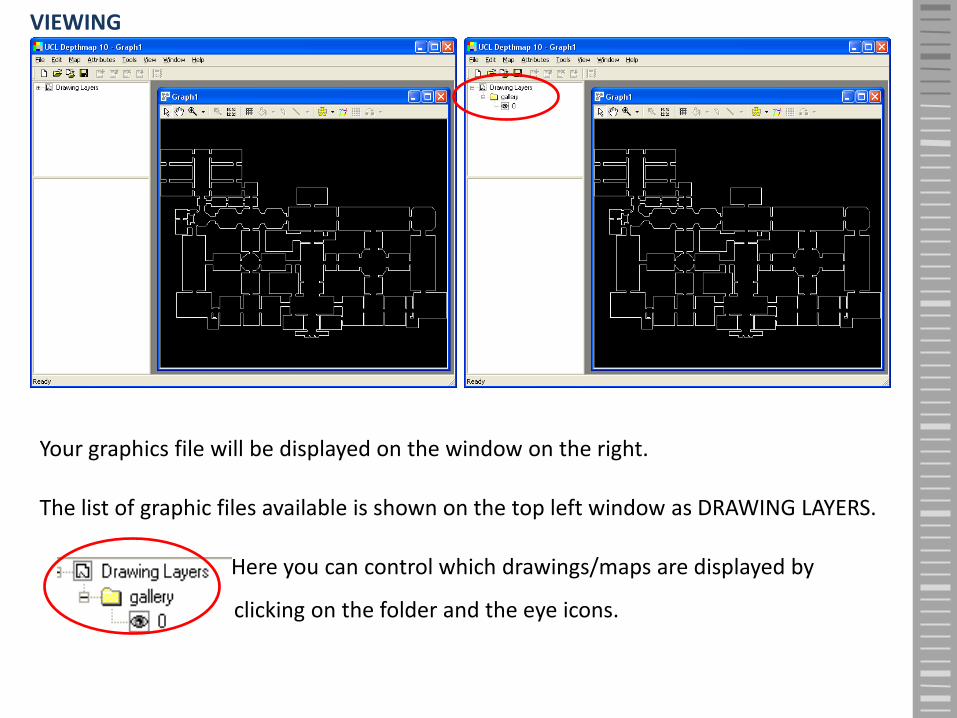
Your graphics file will be displayed on the window on the right.
The list of graphic files available is shown on the top left window as DRAWING LAYERS.
Here you can control which drawings/maps are displayed by
clicking on the folder and the eye icons.
VIEWING
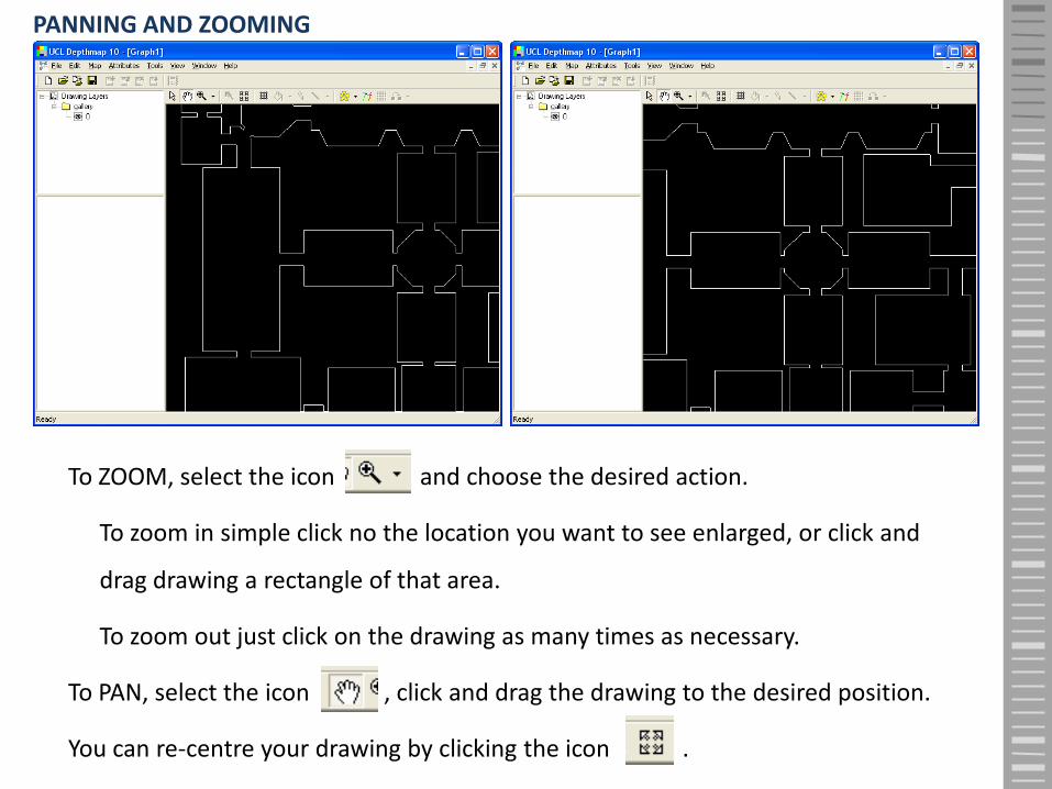
To ZOOM, select the icon and choose the desired action.
To zoom in simple click no the location you want to see enlarged, or click and
drag drawing a rectangle of that area.
To zoom out just click on the drawing as many times as necessary.
To PAN, select the icon , click and drag the drawing to the desired position.
You can re-centre your drawing by clicking the icon .
PANNING AND ZOOMING

To save the Depthmap file you’re working on:
From top menu FILE choose SAVE AS...
Choose the folder where you want to save the file.
Name the file.
Click OK.
FILE → SAVE AS...SAVING A FILE
This part of the tutorial has covered the basic commands of Depthmap, namely opening and importing files, panning, zooming, re-centring the map and saving a file.
Visibility Graph Analysis
Setting the grid
Filling the grid
Creating the graph
Attributes
Step Depth
Isovists
Analysing the graph
This tutorial will show how to perform a VGA analysis of a building layout. In this case an art gallery.
Turner, Alasdair and Doxa, Maria and O'Sullivan, David and Penn, Alan (2001) From isovists to visibility graphs: a methodology for the analysis of architectural space. Environment and Planning B: Planning and Design, 28 (1). pp. 103-121.

Open Depthmap, create new file.
Import file gallery.dxf
Save the Depthmap file you have just created: From top menu FILE choose SAVE AS...
Choose directory and name the file.
FILE → NEW + MAP → IMPORT FILE → SAVE AS
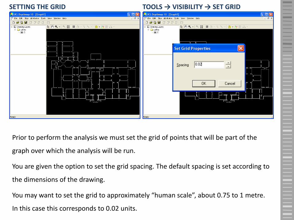
Prior to perform the analysis we must set the grid of points that will be part of the
graph over which the analysis will be run.
You are given the option to set the grid spacing. The default spacing is set according to
the dimensions of the drawing.
You may want to set the grid to approximately “human scale”, about 0.75 to 1 metre.
In this case this corresponds to 0.02 units.
SETTING THE GRID TOOLS → VISIBILITY → SET GRID

Once the grid is set, you can fill it with the fill tool .
The fill tool uses flood to fill the area to analyse with analysis points.
Note that for this tool to work your plan must be closed, otherwise the flood will
reach open areas.
Note that on the list of drawings now there is an item named Visibility Graphs. This is
where the list of your grids for analysis is displayed.
FILLING THE GRID

You can use the pencil tool to make adjustments to your graph.
Use the left mouse button to fill in extra points (adding points to the graph).
Use the right mouse button to delete points.
You can also delete points by selecting them with a click or by dragging creating a
window with the cursor and pressing DEL on the keyboard.
Use Shift key to select more than one range.
FILLING THE GRID - USING THE PENCIL TOOL
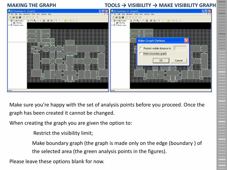
Make sure you’re happy with the set of analysis points before you proceed. Once the
graph has been created it cannot be changed.
When creating the graph you are given the option to:
Restrict the visibility limit;
Make boundary graph (the graph is made only on the edge (boundary ) of
the selected area (the green analysis points in the figures).
Please leave these options blank for now.
MAKING THE GRAPH TOOLS → VISIBILITY → MAKE VISIBILITY GRAPH
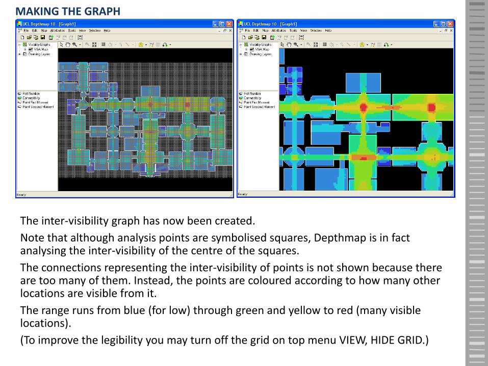
The inter-visibility graph has now been created.
Note that although analysis points are symbolised squares, Depthmap is in fact analysing the inter-visibility of the centre of the squares.
The connections representing the inter-visibility of points is not shown because there are too many of them. Instead, the points are coloured according to how many other locations are visible from it.
The range runs from blue (for low) through green and yellow to red (many visible locations).
(To improve the legibility you may turn off the grid on top menu VIEW, HIDE GRID.)
MAKING THE GRAPH
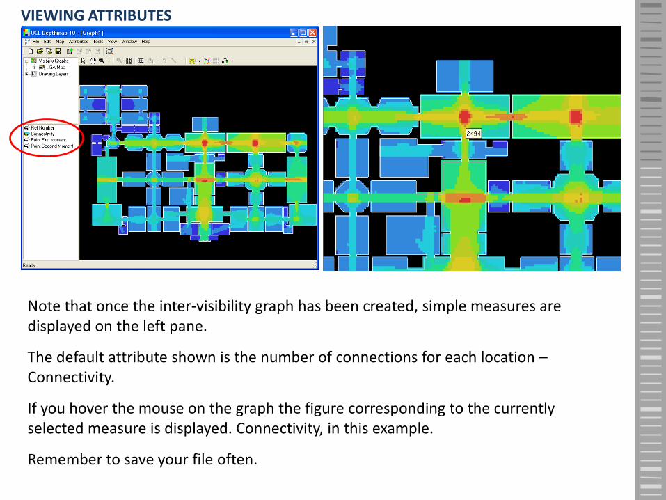
Note that once the inter-visibility graph has been created, simple measures are displayed on the left pane.
The default attribute shown is the number of connections for each location –Connectivity.
If you hover the mouse on the graph the figure corresponding to the currently selected measure is displayed. Connectivity, in this example.
Remember to save your file often.
VIEWING ATTRIBUTES
STEP DEPTH TOOLS → VISIBILITY → STEP DEPTH → VISIBILITY STEP DEPTH
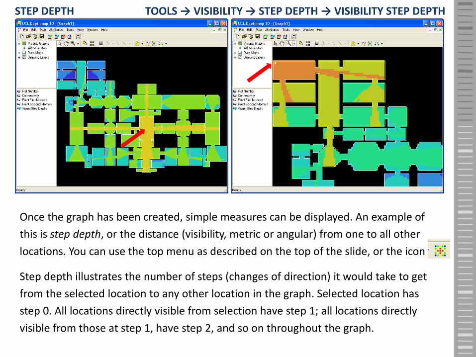
Once the graph has been created, simple measures can be displayed. An example of
this is step depth, or the distance (visibility, metric or angular) from one to all other
locations. You can use the top menu as described on the top of the slide, or the icon
Step depth illustrates the number of steps (changes of direction) it would take to get
from the selected location to any other location in the graph. Selected location has
step 0. All locations directly visible from selection have step 1; all locations directly
visible from those at step 1, have step 2, and so on throughout the graph.

Depthmap can create polygons that represent the potential field of view from a
certain location. These are called ‘isovists’. It is in fact an approximation only.
To create an isovist just click the dropdown menu , choose isovist and click
on the location you want the isovist to be made from.
Some properties of these isovists are automatically calculated and listed on the
bottom left pane.
ISOVISTS

Step depth just shows depth values for one location. If you would like to calculate step
depth to all locations in the graph and be able to compare them to each other, we
must run an analysis on the graph as indicated on the top of the slide (from top menu
TOOLS choose VISIBILITY, then choose RUN VISIBILITY GRAPH ANALYSIS).
On the pop-up window Analysis Options choose ‘Calculate visibility relationships’ to
create the comparative depth measures.
ANALYSING THE GRAPH TOOLS → VISIBILITY → RUN VISIBILITY GRAPH ANALYSIS
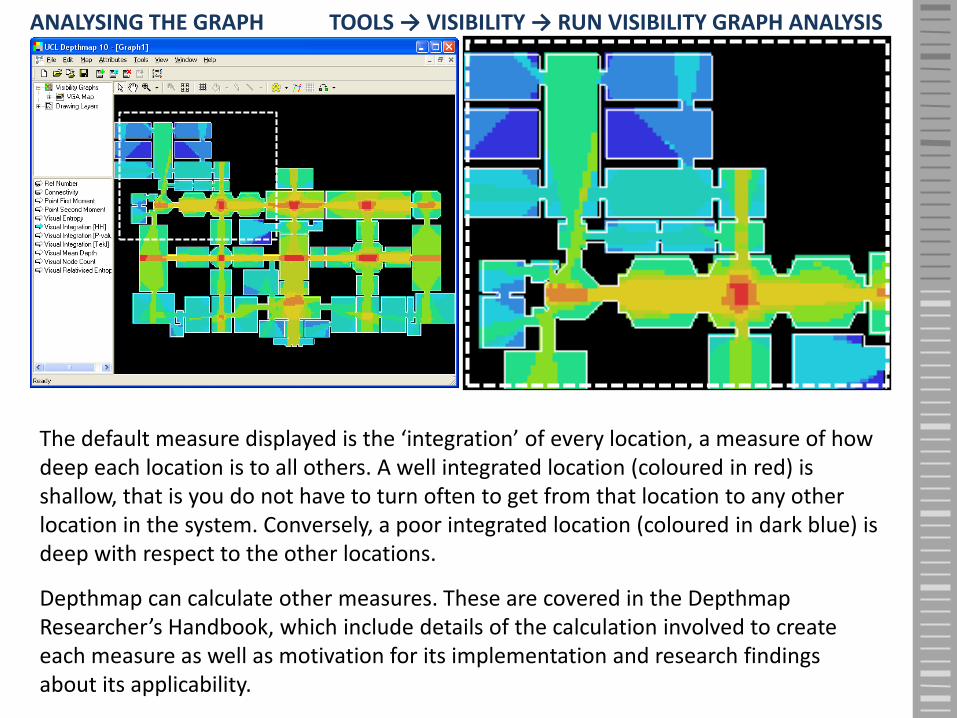
The default measure displayed is the ‘integration’ of every location, a measure of how deep each location is to all others. A well integrated location (coloured in red) is shallow, that is you do not have to turn often to get from that location to any other location in the system. Conversely, a poor integrated location (coloured in dark blue) is deep with respect to the other locations.
Depthmap can calculate other measures. These are covered in the Depthmap Researcher’s Handbook, which include details of the calculation involved to create each measure as well as motivation for its implementation and research findings about its applicability.
ANALYSING THE GRAPH TOOLS → VISIBILITY → RUN VISIBILITY GRAPH ANALYSIS

This part of the tutorial has covered, setting the grid, filling thegrid, creating the graph, choose which attributes to display,calculate step depth, draw isovists and analyse the graph.

Convex Space Analysis
Drawing the convex map
Linking the spaces
Analysing the map
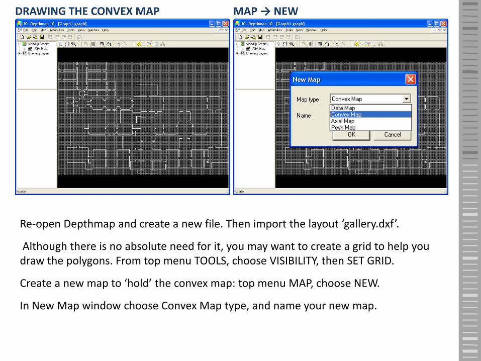
Re-open Depthmap and create a new file. Then import the layout ‘gallery.dxf’.
Although there is no absolute need for it, you may want to create a grid to help you draw the polygons. From top menu TOOLS, choose VISIBILITY, then SET GRID.
Create a new map to ‘hold’ the convex map: top menu MAP, choose NEW.
In New Map window choose Convex Map type, and name your new map.
DRAWING THE CONVEX MAP MAP → NEW

You are now ready to create the polygons.
The icon should already be selected. You can now draw the convex spaces.
To start a polygon, click once with the cross cursor placed where you want to begin. If you wish to align to the grid hold down the Ctrl key while you draw. A small cross will show where the point will snap to when you click.
Move the mouse to the next vertices you want to create and left-click. To close a polygon click roughly in the same position of the first point drawn.
Never double-click, always click only once.
DRAWING THE CONVEX MAP
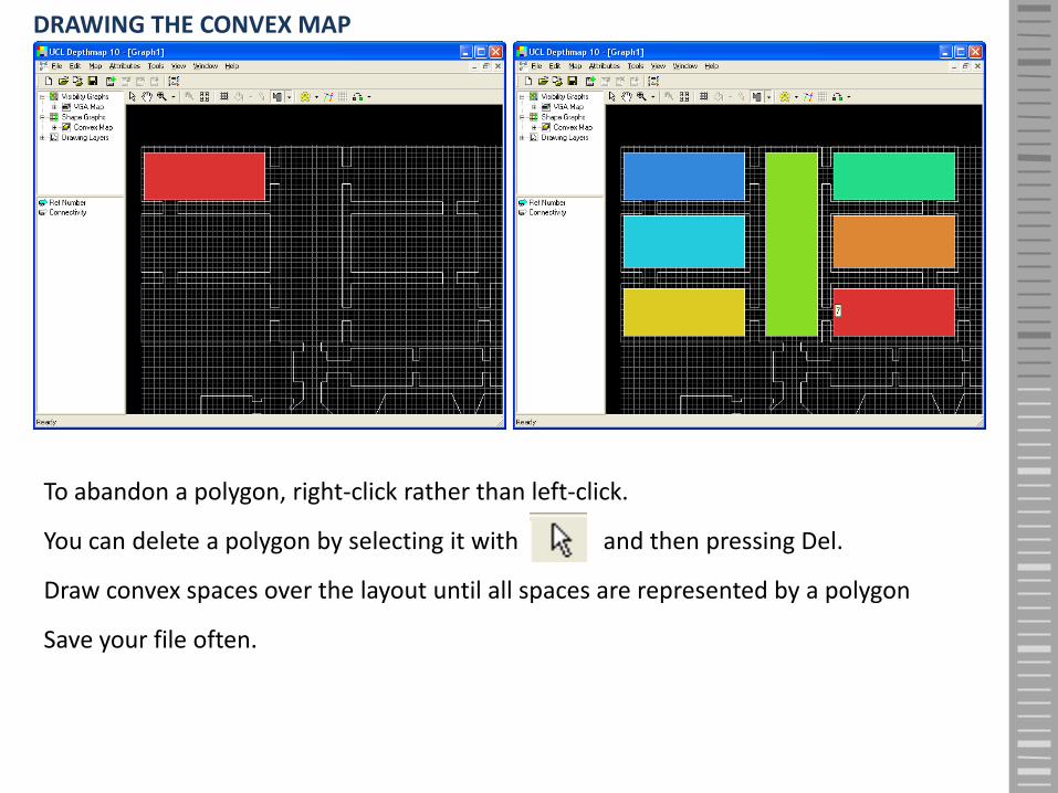
To abandon a polygon, right-click rather than left-click.
You can delete a polygon by selecting it with and then pressing Del.
Draw convex spaces over the layout until all spaces are represented by a polygon
Save your file often.
DRAWING THE CONVEX MAP
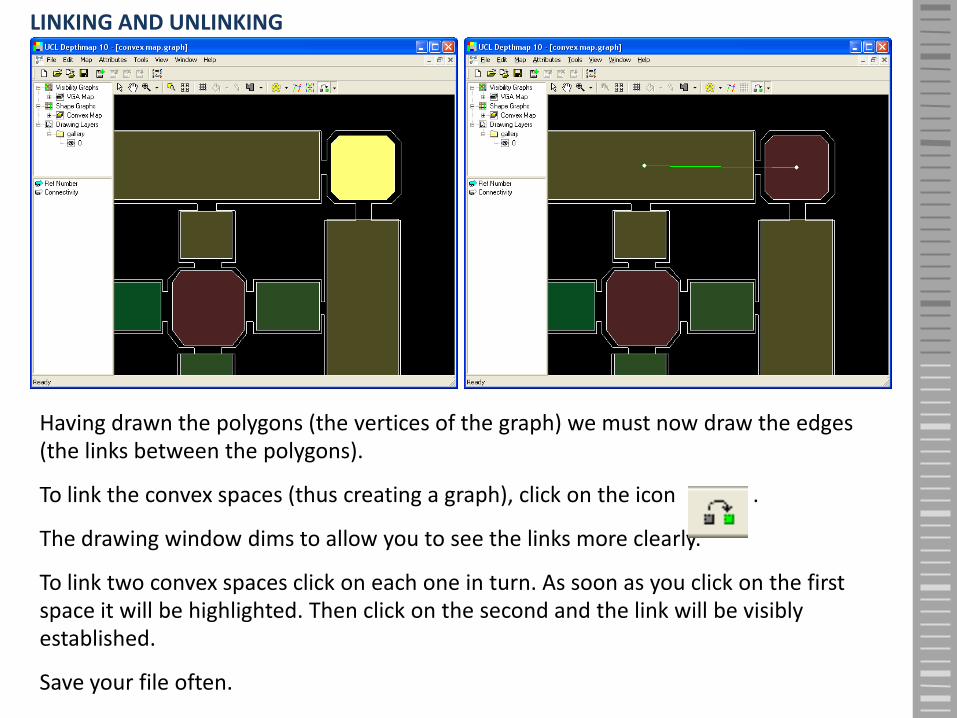
Having drawn the polygons (the vertices of the graph) we must now draw the edges (the links between the polygons).
To link the convex spaces (thus creating a graph), click on the icon .
The drawing window dims to allow you to see the links more clearly.
To link two convex spaces click on each one in turn. As soon as you click on the first space it will be highlighted. Then click on the second and the link will be visibly established.
Save your file often.
LINKING AND UNLINKING

To link two convex spaces click in each one in turn. As soon as you click on the first space it will be highlighted.
Proceed to link all the spaces that adjacent to each other.
To unlink two spaces use the unlink tool from the link pop-down menu, and click on the spaces to unlink in turn.
Save your file often.
LINKING AND UNLINKING
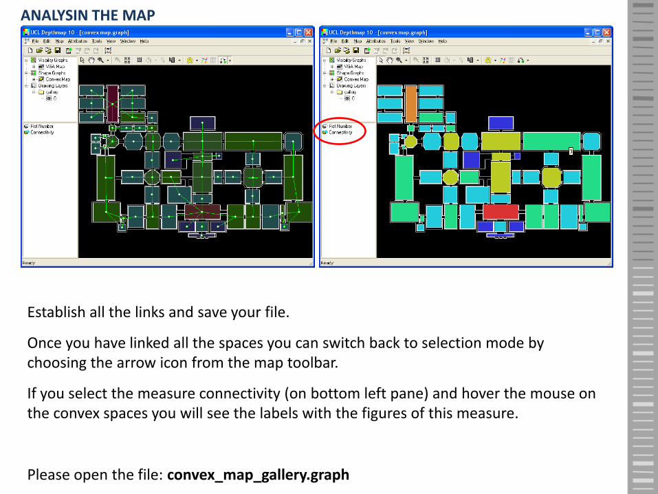
Establish all the links and save your file.
Once you have linked all the spaces you can switch back to selection mode by choosing the arrow icon from the map toolbar.
If you select the measure connectivity (on bottom left pane) and hover the mouse on the convex spaces you will see the labels with the figures of this measure.
Please open the file: convex_map_gallery.graph
ANALYSIN THE MAP

In the same fashion as in VGA, you can analyse step depth by selecting a convex space and then selecting TOOLS from the top menu (as described on the top of the slide).
As with VGA, convex spaces that are one step away from the root space are at depth 1, those two steps away at depth to and so on. Shallow spaces will be coloured red, through to dark blue (deep spaces).
ANALYSIN THE MAP TOOLS → VISIBILITY → STEP DEPTH → VISIBILITY STEP DEPTH
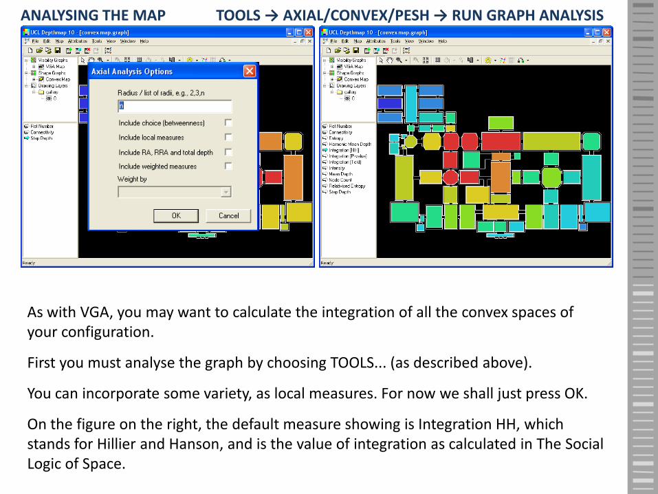
As with VGA, you may want to calculate the integration of all the convex spaces of your configuration.
First you must analyse the graph by choosing TOOLS... (as described above).
You can incorporate some variety, as local measures. For now we shall just press OK.
On the figure on the right, the default measure showing is Integration HH, which stands for Hillier and Hanson, and is the value of integration as calculated in The Social Logic of Space.
ANALYSING THE MAP TOOLS → AXIAL/CONVEX/PESH → RUN GRAPH ANALYSIS

This part of the tutorial has covered drawing a convex map,linking and unlinking spaces, and then analysing it.
For a description of other syntactic measures available pleaserefer to the Depthmap Researcher’s Handbook under thechapter on axial analysis.

Axial Map Analysis
Importing drawing with axial map
Convert drawing to axial map
Automatically create axial map
Analyse the map

If you have a drawing file with the axial map:
Import it; (for this demonstration please import file barnsbury_axial.dxf)
Convert it to axial map: From top menu MAP, choose CONVERT DRAWING MAP.
Choose AXIAL MAP. You may name the file or accept the default name. Click OK.
Notice the new map (Axial Map) listed on the map list on the top left pane.
Your new axial map already has the measure of connectivity. It is now a graph.
IMPORTING/CONVERTING THE MAP MAP → CONVERT DRAWING MAP

If you don’t have a drawing file with the axial map but have a geometrically closed polygon of the layout:
Import the layout;
Create an all-line-axial-map by clicking the icon and clicking inside the polygon to indicate the area to be covered by the map.
AUTOMATIC MAP

Reduce the all-line-map to an axial map. With the command described above: TOOLS...
Notice a new Fewest-Line-Map (minimal) on the top left pane. This is your axial map.
Your new axial map already has the measure of connectivity. It is a graph.
You can now calculate step depth. For other measures it is necessary to run an analysis on the graph.
AUTOMATIC MAP TOOLS → AXIAL/CONVEX... → REDUCE TO FEWEST LINE MAP

Before running an analysis you may make amendments/adjustments to the graph.
As previously done, use icon to link two lines (these can be the lift/staircase between floors on buildings; or ends of tunnel in urban contexts) .
Or use the icon to unlink two lines.
You should also make sure there aren’t isolated lines (or groups of lines) before running the analysis.
UNLINKING/LINKING

When you’re happy with the graph, run the analysis (as described above).
Note the new measures showing on the attributes list (bottom left pane).
You can choose to display any measure.
IMPORTANT: Save this file to use it later on.
ANALYSING THE MAP TOOLS → AXIAL/CONVEX... → RUN GRAPH ANALYSIS
This part of the tutorial has covered importing a drawing of anaxial map and converting it to an axial map, generating anautomatic axial map, linking/unlinking lines, running analysis onthe axial map.
For a description of other syntactic measures available pleaserefer to the Depthmap Researcher’s Handbook under thechapter on axial analysis.
Segment Map Analysis
Converting axial map to segment map
Analysing the map

Segment maps should be created from axial maps. This way they will ‘hold’ the links/unlinks defined.
Open the Depthmap file where you previously analysed an axial map.
Select the Axial Map on the top left pane.
From top menu MAP choose CONVERT DRAWING MAP, choose SEGMENT MAP. (Make sure that the active map is the Axial Map)
A segment map is created and added to the list of maps (top left pane).
CONVERT AXIAL TO SEGMENT MAP MAP → CONVERT ACTIVE MAP

To calculate syntactic measures the graph must be analysed.
From top menu TOOLS choose SEGMENT, then RUN SEGMENT ANALYSIS.
Make sure Tulip is selected
Click include choice (betweenness)
Click metric for radius type. Choose desired radius: walk 400metres or 5 min; 800metres or 10min (the same as cycling 5 min.); 1200 metres imply 15 min. Walking, 7.5 min cycling or 5 min. Driving. (n,200,400,800,1200), for example
Click weighted measures and scroll to segment length. Click OK
ANALYSE SEGMENT MAP TOOLS → SEGMENT → RUN SEGMENT ANALYSIS

Segment map of London _ChoiceR2Km – Space Syntax Ltd

Segment map of London _ChoiceR50Km – Space Syntax Ltd

This part of the tutorial has covered converting an axial map to segment map, and run the analysis on the segment map.

Data Management/Analysis
Maps, Tables and Scatter Plots
Export Maps
Export Tables
Export the Graph

Maps and tables are simply two different views of the same data.
Use the top menu WINDOW to choose the elements you may wish to display (Table, Map, Scatterplot).
From menu WINDOW choose TILE to display the chosen elements simultaneously.
The menu WINDOW also gives you access to COLOUR RANGE. This feature allows you to adjust the colour range of displayed attributes.
MAPS , TABLES AND SCATTERPLOTS

MAPS , TABLES AND SCATTERPLOTS

You can print directly from Depthmap.
Alternatively, you can copy or export the displayed map.
Depthmap can export .eps and .svg file types.
You can then use the image file with other applications. If you copied, the screen (EDIT, COPY SCREEN) just paste it in the desired document (text or image editors).
If you exported the image file, import it to any document (text or image editors).
EXPORT MAPS EDIT → EXPORT SCREEN
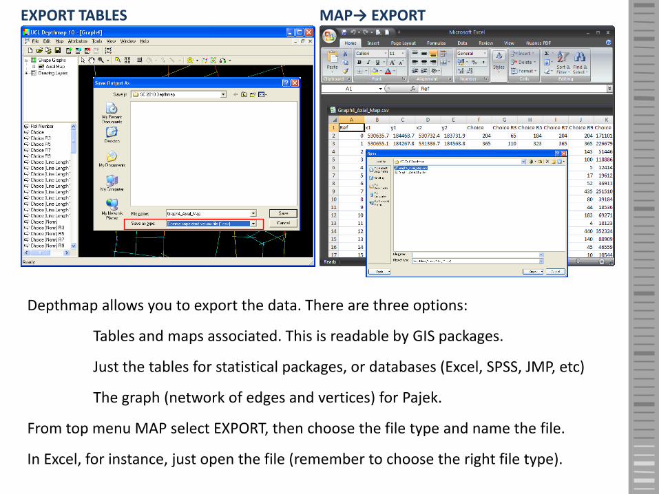
Depthmap allows you to export the data. There are three options:
Tables and maps associated. This is readable by GIS packages.
Just the tables for statistical packages, or databases (Excel, SPSS, JMP, etc)
The graph (network of edges and vertices) for Pajek.
From top menu MAP select EXPORT, then choose the file type and name the file.
In Excel, for instance, just open the file (remember to choose the right file type).
EXPORT TABLES MAP→ EXPORT

In Pajek, just open the file.
EXPORT PAJEK GRAPH MAP→ EXPORT

This part of the tutorial has covered aspects of datamanagement as displaying maps, tables and scatterplots,export maps, tables and the graph to use with geographicinformation systems, text or image editors, statistical andnetwork analysis packages.

Agents
Release agents from selected location
View agents traces and data
Turner, Alasdair and Penn, Alan (2002) Encoding natural movement as an agent-based system: an investigation into human pedestrian behaviour in the built environment. Environment and Planning B: Planning and Design, 29 . pp. 473-490.

Agents are released on a graph, not on a layout per se. The first step is to import a layout (with closed geometry). Second, create a grid and fill it in. There is no need to compute measures though.
Then select a location to release the agents from. Use and click on the graph near the entrance.
Go to TOOLS... (as mentioned above). Choose ‘Release from selected area’. Click OK.
Note a new attribute field ‘Gate counts’ which contains the number of subjects that pass at each location.
RELEASING AGENTS TOOLS → AGENT TOOLS → RUN AGENT ANALYSIS

Conclusion
This tutorial has covered the essentials of Depthmap V10.07.00rincluding VGA, convex analysis, axial analysis, segment analysis, datamanagement/analysis, and agents. You should now have a generalidea of the capabilities of the software as well as of the basicprinciples for using it.
How to get Depthmap
http://www.spacesyntax.org/software/depthmap.asp
Depthmap is free for academic use. You can register to get a license here:
You can also join depthmap’s mailing list where you can get in contact with other users to share experiences, here:
https://www.jiscmail.ac.uk/cgi-bin/webadmin?A0=DEPTHMAP
Other resources available online:
The Depthmap Handbook
http://www.vr.ucl.ac.uk/depthmap/handbook.html
Tutorials (older versions)
http://www.vr.ucl.ac.uk/depthmap/tutorials/
Scripting manual
http://www.vr.ucl.ac.uk/depthmap/scripting/manual.html
Software developer’s kit
http://www.vr.ucl.ac.uk/depthmap/sdk.html
Thank You