introduction to database systems...where we are • motivation for using a dbms for managing data...

1

CSE 344

Lectures 9: Relational Algebra

CSE 344 - Winter 2014

Announcements

• Homework 2 due tonight!

• Homework 3 is posted, due next Thursday!

• Webquiz 3 due tomorrow night!

• Reminder about Discussion Board – Post your question on HW/WQ here

– Feel free to answer your friends’ questions and discuss

concepts (no solution please )

– You can set alert to get email notification

• Today’s lecture: 2.4 and 5.1-5.2 CSE 344 - Winter 2014 2

Where We Are • Motivation for using a DBMS for managing data

• SQL, SQL, SQL

– Declaring the schema for our data (CREATE TABLE)

– Inserting data one row at a time or in bulk (INSERT/.import)

– Modifying the schema and updating the data (ALTER/UPDATE)

– Querying the data (SELECT)

– Tuning queries (CREATE INDEX)

• Next step: More knowledge of how DBMSs work

– Relational algebra and query execution

– Client-server architecture

CSE 344 - Winter 2014 3

Relational Algebra

CSE 344 - Winter 2014 4

Sets v.s. Bags

• Sets: {a,b,c}, {a,d,e,f}, { }, . . .

• Bags: {a, a, b, c}, {b, b, b, b, b}, . . .

Relational Algebra has two semantics:

• Set semantics = standard Relational Algebra

• Bag semantics = extended Relational Algebra

CSE 344 - Winter 2014 5

Relational Algebra Operators

• Union , intersection , difference -

• Selection s

• Projection Π

• Cartesian product , join ⨝

• Rename

• Duplicate elimination d

• Grouping and aggregation g

• Sorting t

CSE 344 - Winter 2014 6

RA

Extended RA

Why learn RA?

• SQL incorporates RA at its center

• When DBMS processes a query, it is

translated into an RA expression

internally and is used by the query

optimizer

• Why Algebra?

7

Why learn RA?

• Why Algebra?

– Has both Operators and Atomic Operands

– (x+y) * (z - 3)

– Similarly,

zip sdisease=‘heart’(Patient))

8

Union and Difference

For set operations, R1 and R2

• must have identical schemas

• their attributes must have the same order,

i.e. R1(A, B) and R2(B, A) is not allowed

R1 R2

R1 – R2

CSE 344 - Winter 2014 9

What about Intersection ?

• Can you derive R1 R2 using

union/minus?

CSE 344 - Winter 2014 10

R1 R2

R2 – (R2 – R1)

R1 – (R1 – R2)

(R1 U R2) – ((R1 U R2) –

R1) - ((R1 U R2) – R2)

What about Intersection ?

• Derived operator using minus

• Derived using join (will explain later)

R1 R2 = R1 – (R1 – R2)

R1 R2 = R1 ⨝ R2

CSE 344 - Winter 2014 11

Union, Difference, Intersection

over Bags

R1 R2

R1 – R2

R1 R2

CSE 344 - Winter 2014 12

What do they mean over bags ?

A

1

1

1

A

1

1

R1 R2

How many 1’s in

• R1 R2: 5

• R1 – R2: 1

• R2 – R1: 0

•R1 R2: 2

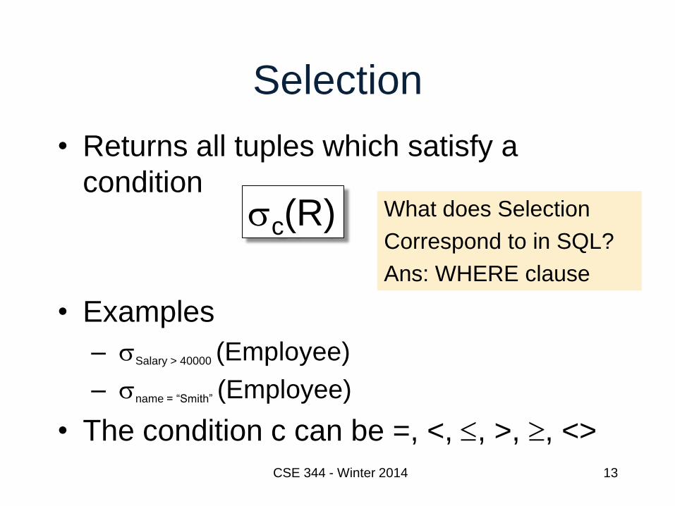
Selection

• Returns all tuples which satisfy a

condition

• Examples

– sSalary > 40000 (Employee)

– sname = “Smith” (Employee)

• The condition c can be =, <, , >, , <>

sc(R)

CSE 344 - Winter 2014 13

What does Selection

Correspond to in SQL?

Ans: WHERE clause

sSalary > 40000 (Employee)

SSN Name Salary

1234545 John 200000

5423341 Smith 600000

4352342 Fred 500000

SSN Name Salary

5423341 Smith 600000

4352342 Fred 500000

Employee

CSE 344 - Winter 2014 14

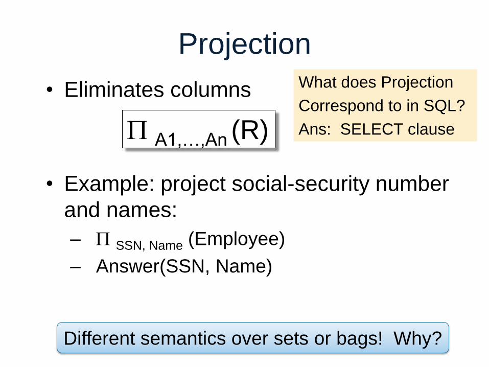
Projection

• Eliminates columns

• Example: project social-security number

and names:

– P SSN, Name (Employee)

– Answer(SSN, Name)

P A1,…,An (R)

CSE 344 - Winter 2014 15 Different semantics over sets or bags! Why?

What does Projection

Correspond to in SQL?

Ans: SELECT clause

P Name,Salary (Employee)

SSN Name Salary

1234545 John 20000

5423341 John 60000

4352342 John 20000

Name Salary

John 20000

John 60000

John 20000

Employee

Name Salary

John 20000

John 60000

Bag semantics Set semantics

Which is more efficient? Ans: Bag

Checking and removing duplicates is expensive 16


Composing RA Operators

no name zip disease

1 p1 98125 flu

2 p2 98125 heart

3 p3 98120 lung

4 p4 98120 heart

Patient

sdisease=‘heart’(Patient)

no name zip disease

2 p2 98125 heart

4 p4 98120 heart

zip disease

98125 flu

98125 heart

98120 lung

98120 heart

zip,disease(Patient)

zip sdisease=‘heart’(Patient))

zip

98120

98125

17

Cartesian/Cross Product

• Each tuple in R1 with each tuple in R2

• Rare in practice; mainly used to express

joins

R1 R2

CSE 344 - Winter 2014 18

Name SSN

John 999999999

Tony 777777777

Employee

EmpSSN DepName

999999999 Emily

777777777 Joe

Dependent

Employee � Dependent

Name SSN EmpSSN DepName

John 999999999 999999999 Emily

John 999999999 777777777 Joe

Tony 777777777 999999999 Emily

Tony 777777777 777777777 Joe

Cross-Product Example

CSE 344 - Winter 2014 19

Disambiguate

attributes if necessary

Employee.EmpSSN

Dependent.EmpSSN

Renaming

• Changes the schema, not the instance

• Example:

– N, S(Employee) Answer(N, S)

– Given R(A, B)

S(R) : Renamed relation S(A, B)

S(X,Y)(R) or S= X,Y(R): Renamed relation S(X, Y)

Sometimes written as S = A->X, B->Y(R)

B1,…,Bn (R)

20 Not really used by systems, but needed on paper

Natural Join

• Meaning: R1⨝ R2 = PA(s(R1 × R2))

• Where:

– Selection s checks equality of all common attributes

– Projection eliminates duplicate common attributes

CSE 344 - Winter 2014 21

R1 ⨝ R2

Natural Join Example A B

X Y

X Z

Y Z

Z V

B C

Z U

V W

Z V

A B C

X Z U

X Z V

Y Z U

Y Z V

Z V W

R S

R ⨝ S =

PABC(sR.B=S.B(R × S))

CSE 344 - Winter 2014 22


Natural Join Example 2

age zip disease

54 98125 heart

20 98120 flu

AnonPatient P Voters V

P V

name age zip

p1 54 98125

p2 20 98120

age zip disease name

54 98125 heart p1

20 98120 flu p2

23

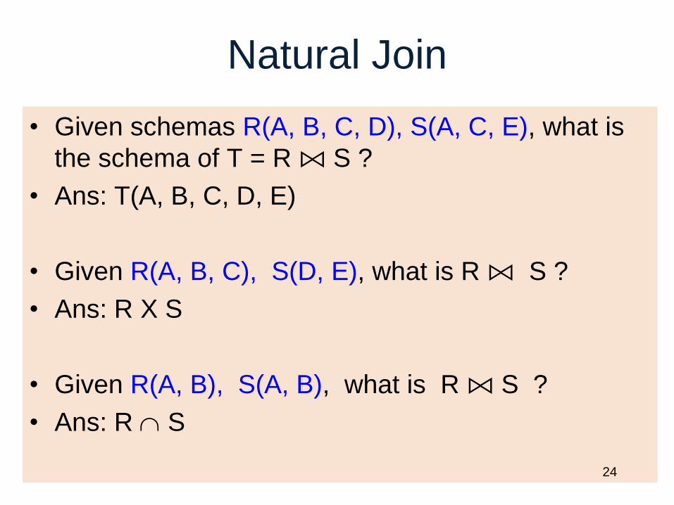
Natural Join

• Given schemas R(A, B, C, D), S(A, C, E), what is

the schema of T = R ⨝ S ?

• Ans: T(A, B, C, D, E)

• Given R(A, B, C), S(D, E), what is R ⨝ S ?

• Ans: R X S

• Given R(A, B), S(A, B), what is R ⨝ S ?

• Ans: R S

24

Theta Join

• A join that involves a predicate

• Here q can be any condition

• For our voters/disease example:

R1 ⨝q R2 = s q (R1 R2)

P ⨝ P.zip = V.zip and P.age < V.age + 5 and P.age > V.age - 5 V

25 CSE 344 - Winter 2014

Equijoin

• A theta join where q is an equality

• This is by far the most used variant of

join in practice

R1 ⨝A=B R2 = sA=B (R1 R2)

CSE 344 - Winter 2014 26


Equijoin Example

age zip disease

54 98125 heart

20 98120 flu

AnonPatient P Voters V

P P.age=V.age V

name age zip

p1 54 98125

p2 20 98120

age P.zip disease name V.zip

54 98125 heart p1 98125

20 98120 flu p2 98120

27


Join Summary

• Theta-join: R q S = sq(R x S)

– Join of R and S with a join condition q

– Cross-product followed by selection q

• Equijoin: R q S = A (sq(R x S))

– Join condition q consists only of equalities

– Projection A drops all redundant attributes

• Natural join: R S = A (sq(R x S))

– Equijoin

– Equality on all fields with same name in R and in S

28

So Which Join Is It ?

• When we write R ⨝ S we usually mean

an equijoin, but we often omit the

equality predicate when it is clear from

the context

CSE 344 - Winter 2014 29


More Joins

• Outer join

– Include tuples with no matches in the output

– Use NULL values for missing attributes

• Variants

– Left outer join

– Right outer join

– Full outer join

30


Outer Join Example

age zip disease

54 98125 heart

20 98120 flu

33 98120 lung

AnonPatient P

P ⋉ V

age zip disease job

54 98125 heart lawyer

20 98120 flu cashier

33 98120 lung null

31

AnnonJob J

job age zip

lawyer 54 98125

cashier 20 98120


Some Examples

Supplier(sno,sname,scity,sstate)

Part(pno,pname,psize,pcolor)

Supply(sno,pno,qty,price)

Q2: Name of supplier of parts with size greater than 10

sname(Supplier Supply (spsize>10 (Part))

Q3: Name of supplier of red parts or parts with size greater than 10

sname(Supplier Supply (spsize>10 (Part) spcolor=‘red’ (Part) ) )

32

CSE 344 - Winter 2014 33

From SQL to RA

34

From SQL to RA

SELECT DISTINCT x.name, z.name

FROM Product x, Purchase y, Customer z

WHERE x.pid = y.pid and y.cid = z.cid and

x.price > 100 and z.city = ‘Seattle’


Product(pid, name, price)

Purchase(pid, cid, store)

Customer(cid, name, city)

35

From SQL to RA

Product Purchase

pid=pid

price>100 and city=‘Seattle’

x.name,z.name

δ

cid=cid

Customer

Π

σ

Product(pid, name, price)

Purchase(pid, cid, store)

Customer(cid, name, city)





36

From SQL to RA

Product Purchase

pid=pid

price>100 and city=‘Seattle’

x.name,z.name

δ

cid=cid

Customer

Π

σ





Can you optimize

this query plan?

37

An Equivalent Expression

Product Purchase

pid=pid

city=‘Seattle’

x.name,z.name

δ

cid=cid

Customer

Π

σ price>100

σ

Query optimization =

finding cheaper,

equivalent expressions

END OF LECTURE09

Extended RA: Operators on

Bags

• Duplicate elimination d

• Grouping g

• Sorting t

CSE 344 - Winter 2014 38

39

Logical Query Plan

SELECT city, count(*)

FROM sales

GROUP BY city

HAVING sum(price) > 100

sales(product, city, price)

g city, sum(price)→p, count(*) → c

s p > 100

P city, c

T1(city,p,c)

T2(city,p,c)

T3(city, c)

T1, T2, T3 = temporary tables



Typical Plan for Block (1/2)

R S

join condition

s selection condition

fields

join condition

…

SELECT-PROJECT-JOIN

Query

40


Typical Plan For Block (2/2)

fields

g fields, sum/count/min/max(fields)

havingcondition

s selection condition

join condition

… … 41


How about Subqueries?

SELECT Q.sno

FROM Supplier Q

WHERE Q.sstate = ‘WA’

and not exists

(SELECT *

FROM Supply P

WHERE P.sno = Q.sno

and P.price > 100)

42



Supply(sno,pno,price)

SELECT Q.sno

FROM Supplier Q


and not exists

(SELECT *

FROM Supply P

WHERE P.sno = Q.sno

and P.price > 100)



43

Correlation !






SELECT Q.sno

FROM Supplier Q


and not exists

(SELECT *

FROM Supply P

WHERE P.sno = Q.sno

and P.price > 100)

44

De-Correlation

SELECT Q.sno

FROM Supplier Q


and Q.sno not in

(SELECT P.sno

FROM Supply P

WHERE P.price > 100)





45

Un-nesting

SELECT Q.sno

FROM Supplier Q


and Q.sno not in

(SELECT P.sno

FROM Supply P


(SELECT Q.sno

FROM Supplier Q

WHERE Q.sstate = ‘WA’)

EXCEPT

(SELECT P.sno

FROM Supply P





EXCEPT = set difference




Supply

ssstate=‘WA’

Supplier

sPrice > 100

46

(SELECT Q.sno

FROM Supplier Q

WHERE Q.sstate = ‘WA’)

EXCEPT

(SELECT P.sno

FROM Supply P


−




Finally…

sno sno

CSE 344 - Winter 2014 47

From Logical Plans

to Physical Plans

Example

CSE 344 - Winter 2014 48

SELECT sname

FROM Supplier x, Supply y

WHERE x.sid = y.sid

and y.pno = 2

and x.scity = ‘Seattle’

and x.sstate = ‘WA’

Give a relational algebra expression for this query

Supplier(sid, sname, scity, sstate)

Supply(sid, pno, quantity)

Relational Algebra

CSE 344 - Winter 2014 49

sname(s scity=‘Seattle’ sstate=‘WA’ pno=2 (Supplier sid = sid Supply))



50

Supplier Supply

sid = sid

s scity=‘Seattle’ sstate=‘WA’ pno=2

sname

Relational Algebra


Relational algebra expression is

also called the “logical query

plan”



51

Physical Query Plan 1

Supplier Supply

sid = sid

s scity=‘Seattle’ sstate=‘WA’ pno=2

sname

(File scan) (File scan)

(Block-nested loop)

(On the fly)

(On the fly)


A physical query plan is a logical

query plan annotated with

physical implementation details



52

Supplier Supply

sid = sid

a s scity=‘Seattle’ sstate=‘WA’

sname

(File scan) (File scan)

(Sort-merge join)

(Scan

write to T2)

(On the fly)

b s pno=2

(Scan

write to T1)


c

d




Supply Supplier

sid = sid

s scity=‘Seattle’ sstate=‘WA’

sname

(Index nested loop)

(Index lookup on sid)

Doesn’t matter if clustered or not

(On the fly)

a s pno=2

(Index lookup on pno )

Assume: clustered


(Use index)

b

c

d

(On the fly)

53




Physical Data Independence

• Means that applications are insulated from

changes in physical storage details

– E.g., can add/remove indexes without changing apps

– Can do other physical tunings for performance

• SQL and relational algebra facilitate physical

data independence because both languages

are “set-at-a-time”: Relations as input and

output

CSE 344 - Winter 2014 54

introduction to database systems...where we are • motivation for using a dbms for managing data...

Documents