introduction to data mining -...
TRANSCRIPT

Introduction to Data Mining
David Banks
Institute of Statistics & Decision Sciences
Duke University
1
Abstract
This shortcourse begins with an introductory overview of data mining: its scope,
classical approaches, and the heuristics that guided the initial development of theory
and methods. Then the course moves towards the treatment of more modern issues
such as boosting, overcompleteness, and large-p-small-n problems. This leads to a
survey of currently popular techniques, including random forests, support vector
machines, and wavelets. The main focus is upon regression inference, as this is a
paradigm that informs all data mining applications, but we also discuss clustering,
classification, and multidimensional scaling. The only prerequisites for the course are
a basic knowledge of applied multivariate inference and a general level of statistical
knowledge comparable to a strong master’s degree. Any math will focus upon
conveying general insight rather than specific details.
2
0. Table of Contents
1. Background and Overview: Nonparametric Regression, Cross-Validation, the
Bootstrap
2. Key Ideas and Methods: Smoothing, Bias-Variance Tradeoff
3. Search and Variable Selection: Experimental Design, Gray Codes, Fitness
4. Nonparametric Regression: Heuristics on Eight Methods
5. Comparing Methods: Designing Experiments in Data Mining
6. Local Dimension: How to Pick Problems Wisely
7. Classification: Boosting, Random Forests, Support Vector Machines
8. Cluster Analysis: Hierarchical, k-Means, and Mixture Models; SOMs
9. Issues with Bases: Hilbert Space, Shrinkage, Overcompleteness
10. Wavelets: Introduction, Construction, Examples
11. Structure Extraction: Regression, Multidimensional Scaling, and Performance
Bounds
3

1. Background and Overview
Data mining tries to find hidden structure in large, high-dimensional datasets.
Interesting structure can arise in regression analysis, discriminant analysis, cluster
analysis, or more exotic situations, such as multidimensional scaling.
Classic applications include:
• Regression models for climate change, wine price, cost of software development.
• Classification models for fraudulent credit card transactions and good credit risk.
• Cluster analyses for market segmentation and microarray data.
• Multidimensional scaling analyses for document retrieval systems.
4
Data mining grew at the interface of statistics, computer science, and database
management.
• Statistical work began in the 1980s, with the invention of CART, and expanded
through increased research on visualization, nonparametric regression, and data
quality.
• Computer scientists coined the term data mining, pioneered neural nets, pursued
aggressive analysis of high-profile problems, and developed a body of ad hoc
techniques.
• Database scientists developed SQL, relational databases, and other key tools.
Data mining has become an important research area, and was the topic of a year-long
program at the Statistical and Applied Mathematical Sciences Institute, 2003-2004.
That program was the impetus to the development of this shortcourse.
5
1.1 Example: Nonparametric Regression
Nonparametric regression is a natural way to introduce the main ideas in data mining.
The core model is
y = f(x) + ε
where x ∈ IRp and f is unknown. The emphasis is upon estimating the function f .
In real problems one observes {yi,xi}, i = 1, . . . , n. We assume that:
• the xi are measured without error
• the εi are i.i.d. with mean zero
• the variance of the εi values is an unknown constant σ.
These are the minor assumptions, and can be weakened in customary ways.
6
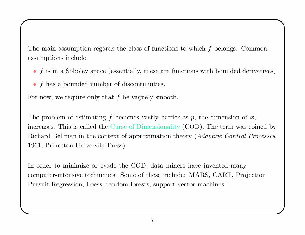
The main assumption regards the class of functions to which f belongs. Common
assumptions include:
• f is in a Sobolev space (essentially, these are functions with bounded derivatives)
• f has a bounded number of discontinuities.
For now, we require only that f be vaguely smooth.
The problem of estimating f becomes vastly harder as p, the dimension of x,
increases. This is called the Curse of Dimensionality (COD). The term was coined by
Richard Bellman in the context of approximation theory (Adaptive Control Processes,
1961, Princeton University Press).
In order to minimize or evade the COD, data miners have invented many
computer-intensive techniques. Some of these include: MARS, CART, Projection
Pursuit Regression, Loess, random forests, support vector machines.
7
The COD applies to all multivariate analyses that choose not to impose strong
modeling assumptions (e.g., that the relationship between x and IE[Y ] is linear, or
that f belongs to a particular parametric family of curves).
Although we use regression as our example, the COD applies equally to classification,
cluster analysis, and multidimensional scaling.
In terms of the sample size n and dimension p, the COD has three nearly equivalent
descriptions:
• For fixed n, as p increases, the data become sparse.
• As p increases, the number of possible models explodes.
• For large p, most datasets are multicollinear (or concurve, which is a
nonparametric generalization).
8
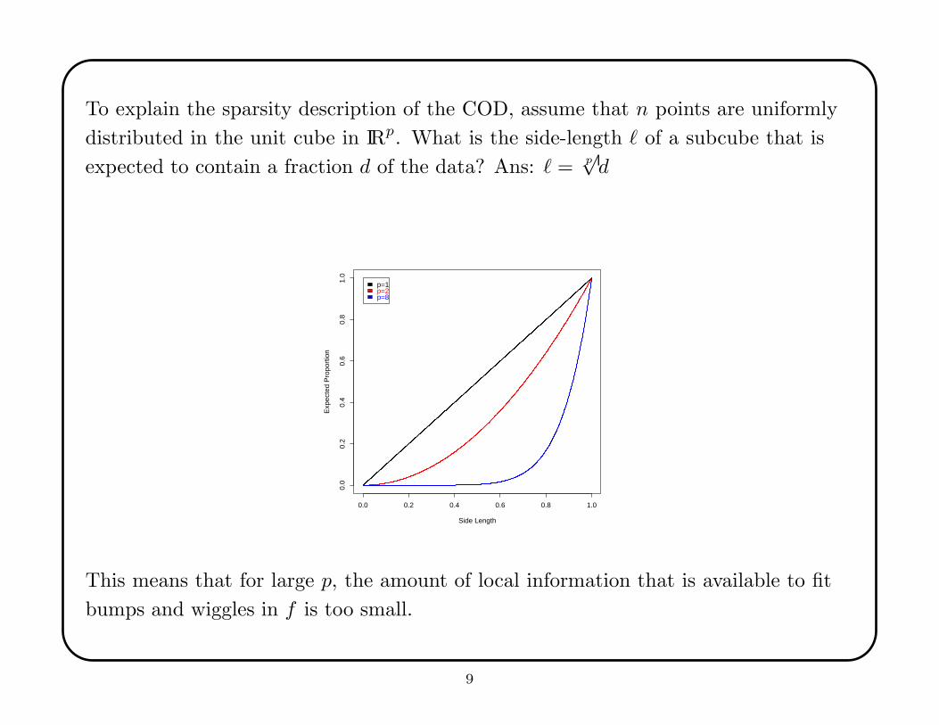
To explain the sparsity description of the COD, assume that n points are uniformly
distributed in the unit cube in IRp. What is the side-length ` of a subcube that is
expected to contain a fraction d of the data? Ans: ` = p√d
0.0 0.2 0.4 0.6 0.8 1.0
0.0
0.2
0.4
0.6
0.8
1.0
Side Length
Exp
ecte
d P
ropo
rtio
n
p=1p=2p=8
This means that for large p, the amount of local information that is available to fit
bumps and wiggles in f is too small.
9
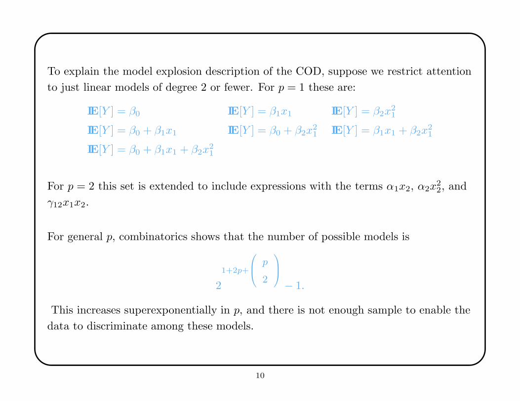
To explain the model explosion description of the COD, suppose we restrict attention
to just linear models of degree 2 or fewer. For p = 1 these are:
IE[Y ] = β0 IE[Y ] = β1x1 IE[Y ] = β2x21
IE[Y ] = β0 + β1x1 IE[Y ] = β0 + β2x21 IE[Y ] = β1x1 + β2x
21
IE[Y ] = β0 + β1x1 + β2x21
For p = 2 this set is extended to include expressions with the terms α1x2, α2x22, and
γ12x1x2.
For general p, combinatorics shows that the number of possible models is
2
1+2p+
0
B
@
p
2
1
C
A
− 1.
This increases superexponentially in p, and there is not enough sample to enable the
data to discriminate among these models.
10
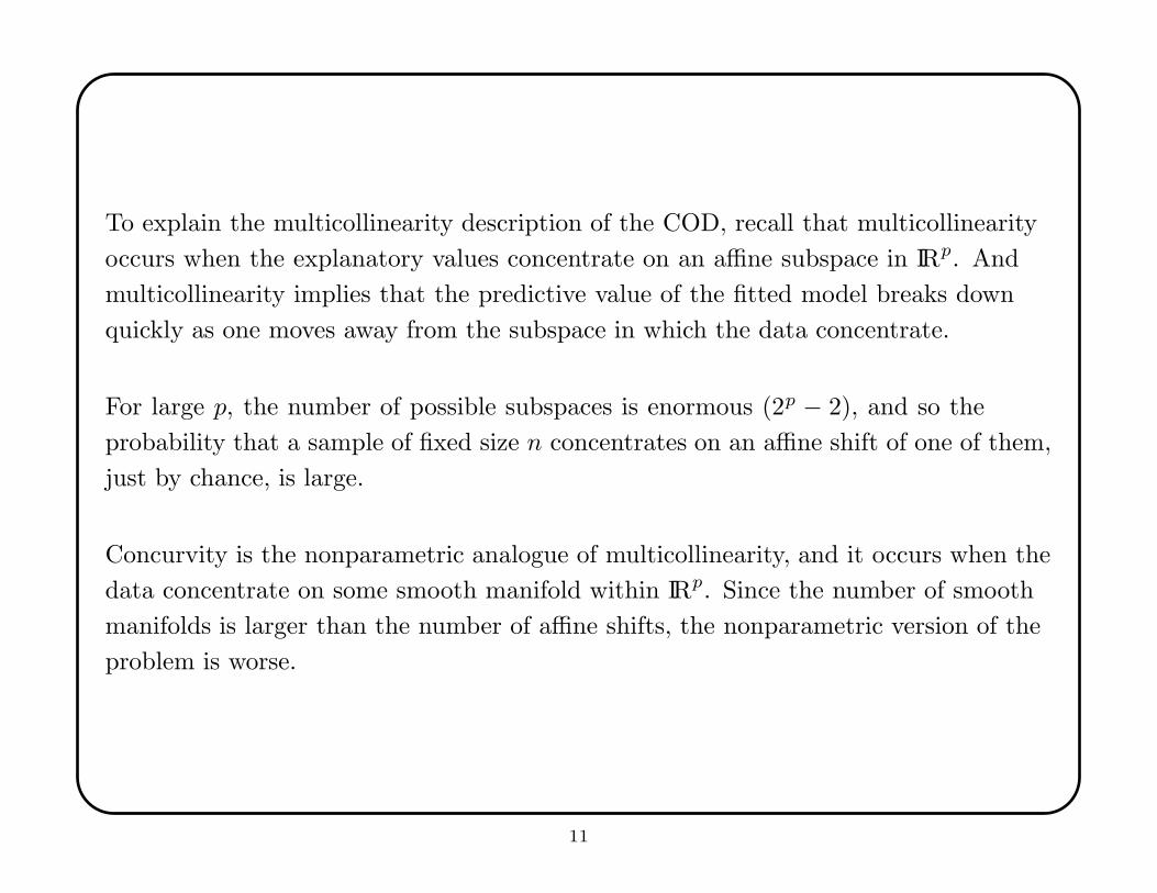
To explain the multicollinearity description of the COD, recall that multicollinearity
occurs when the explanatory values concentrate on an affine subspace in IRp. And
multicollinearity implies that the predictive value of the fitted model breaks down
quickly as one moves away from the subspace in which the data concentrate.
For large p, the number of possible subspaces is enormous (2p − 2), and so the
probability that a sample of fixed size n concentrates on an affine shift of one of them,
just by chance, is large.
Concurvity is the nonparametric analogue of multicollinearity, and it occurs when the
data concentrate on some smooth manifold within IRp. Since the number of smooth
manifolds is larger than the number of affine shifts, the nonparametric version of the
problem is worse.
11
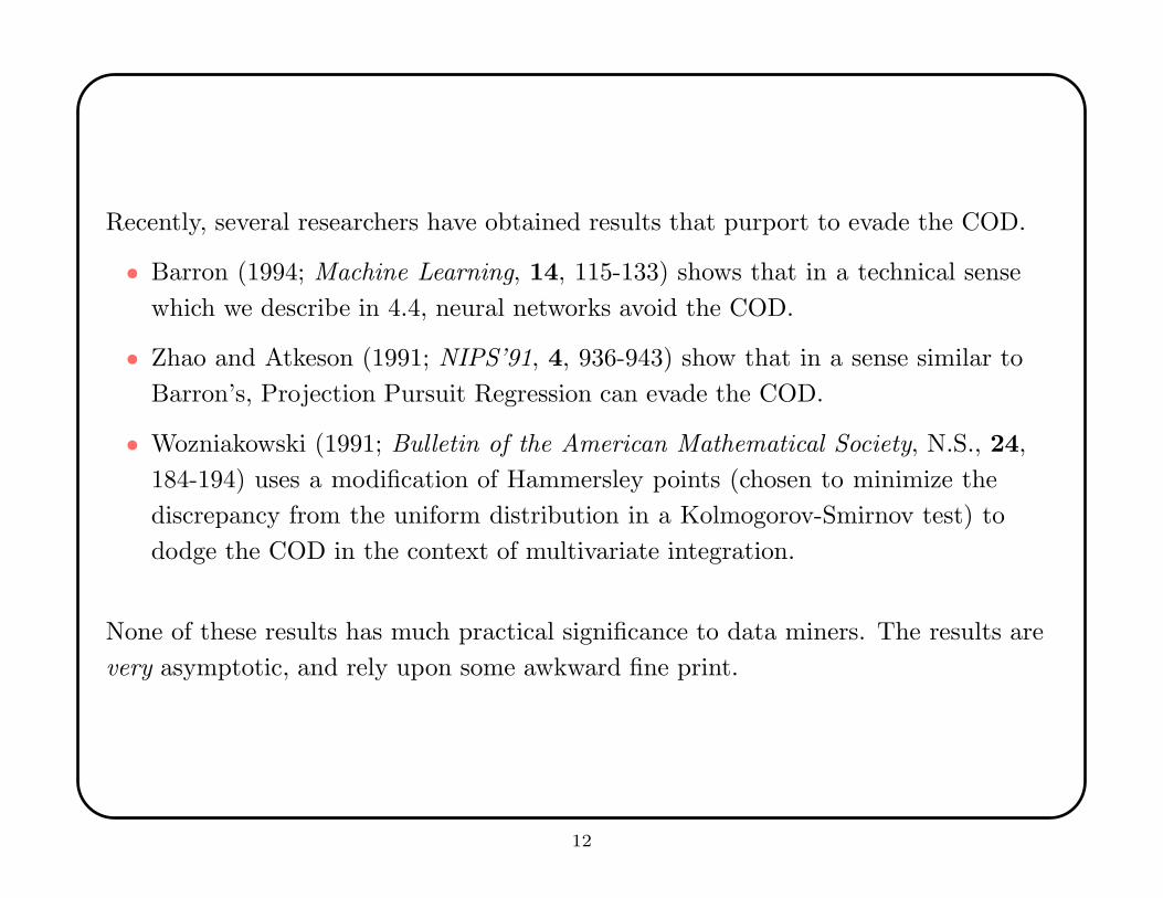
Recently, several researchers have obtained results that purport to evade the COD.
• Barron (1994; Machine Learning, 14, 115-133) shows that in a technical sense
which we describe in 4.4, neural networks avoid the COD.
• Zhao and Atkeson (1991; NIPS’91, 4, 936-943) show that in a sense similar to
Barron’s, Projection Pursuit Regression can evade the COD.
• Wozniakowski (1991; Bulletin of the American Mathematical Society, N.S., 24,
184-194) uses a modification of Hammersley points (chosen to minimize the
discrepancy from the uniform distribution in a Kolmogorov-Smirnov test) to
dodge the COD in the context of multivariate integration.
None of these results has much practical significance to data miners. The results are
very asymptotic, and rely upon some awkward fine print.
12
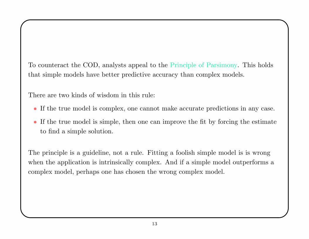
To counteract the COD, analysts appeal to the Principle of Parsimony. This holds
that simple models have better predictive accuracy than complex models.
There are two kinds of wisdom in this rule:
• If the true model is complex, one cannot make accurate predictions in any case.
• If the true model is simple, then one can improve the fit by forcing the estimate
to find a simple solution.
The principle is a guideline, not a rule. Fitting a foolish simple model is is wrong
when the application is intrinsically complex. And if a simple model outperforms a
complex model, perhaps one has chosen the wrong complex model.
13

1.2 Two Tools
In regression, classification, and (often) clustering, there are two key tasks:
• Assessment of model fit.
• Estimation of uncertainty.
The first problem is handled by some variant of cross-validation. The second problem
is handled by the bootstrap.
Both cross-validation and bootstrapping are key methodologies in data mining, and
we review them briefly.
14
1.2.1 Cross-Validation
To assess model fit in complex, computer-intensive situations, the ideal strategy is to
hold out a random portion of the data, fit a model to the rest, then use the fitted
model to predict the response values from the values of the explanatory variables in
the hold-out sample.
This allows a straightforward estimate of predicted mean squared error (PMSE) for
regression, or predictive classification error, or some similar fit criterion. But this
wastes data.
Also, we usually need to compare fits among many models. If the same hold-out
sample is re-used, then the comparisons are not independent and (worse) the model
selection process will tend to choose a model the overfits the hold-out sample, causing
spurious optimism.
15
Cross-validation is a procedure that balances the need to use data to select a model
and the need to use data to assess prediction.
Specifically, v-fold cross-validation is as follows:
• randomly divide the sample into v portions;
• for i = 1, . . . , v, hold out portion i and fit the model from the rest of the data;
• for i = 1, . . . , v, use the fitted model to predict the hold-out sample;
• average the PMSE over the v different fits.
One repeats these steps (including the random division of the sample!) each time a
new model is assessed.
The choice of v requires judgment. If v = n, then cross-validation has low bias but
possibly high variance, and computation is lengthy. If v is small, say 4, then bias can
be large. A common choice is 10-fold cross-validation.
16

Intentional blank.
17

Intentional blank.
18
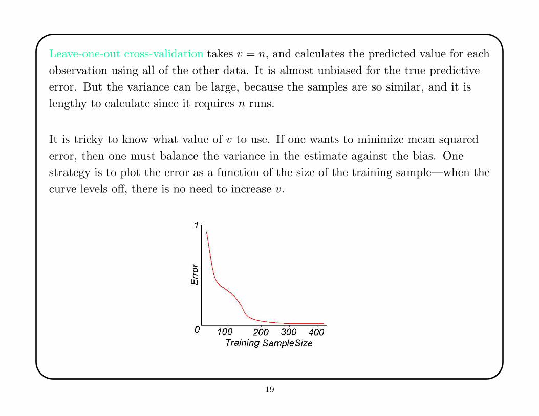
Leave-one-out cross-validation takes v = n, and calculates the predicted value for each
observation using all of the other data. It is almost unbiased for the true predictive
error. But the variance can be large, because the samples are so similar, and it is
lengthy to calculate since it requires n runs.
It is tricky to know what value of v to use. If one wants to minimize mean squared
error, then one must balance the variance in the estimate against the bias. One
strategy is to plot the error as a function of the size of the training sample—when the
curve levels off, there is no need to increase v.
19
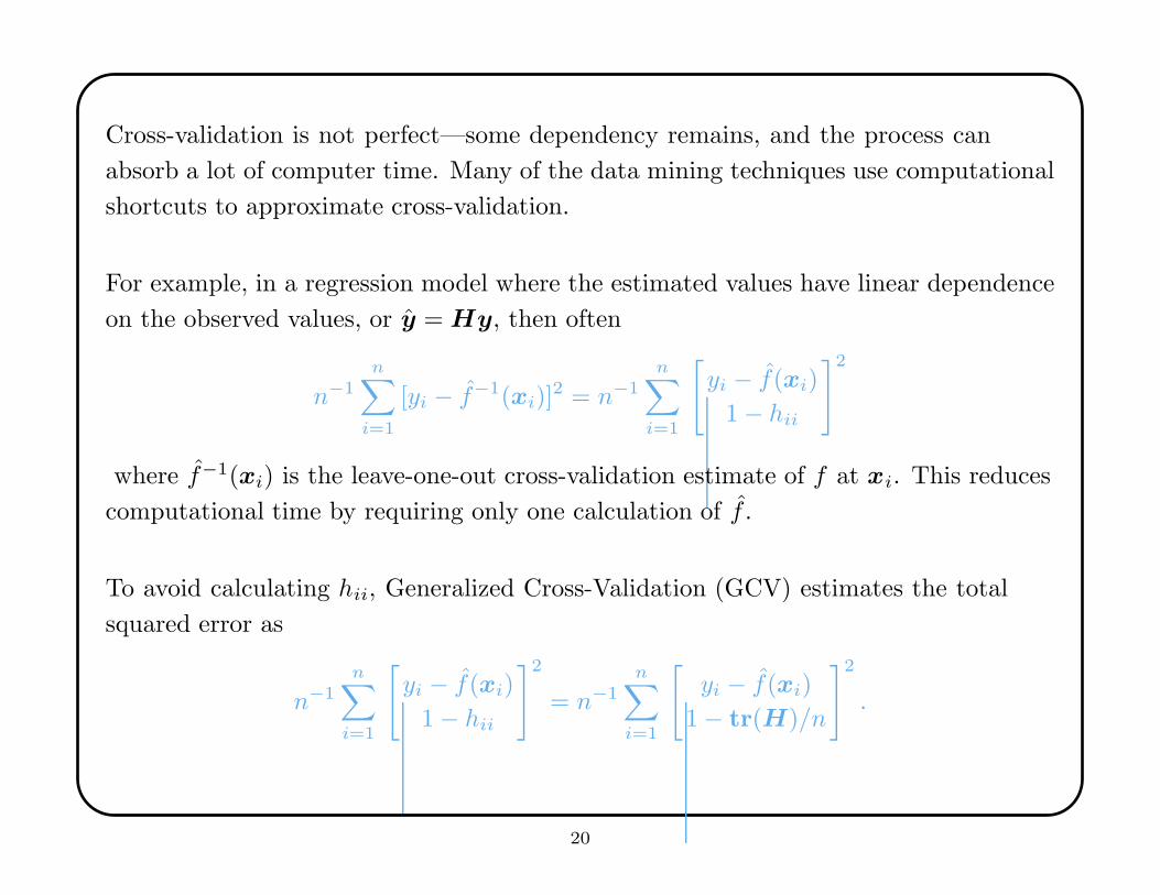
Cross-validation is not perfect—some dependency remains, and the process can
absorb a lot of computer time. Many of the data mining techniques use computational
shortcuts to approximate cross-validation.
For example, in a regression model where the estimated values have linear dependence
on the observed values, or y = Hy, then often
n−1n∑
i=1
[yi − f−1(xi)]2 = n−1
n∑
i=1
[
yi − f(xi)
1 − hii
]2
where f−1(xi) is the leave-one-out cross-validation estimate of f at xi. This reduces
computational time by requiring only one calculation of f .
To avoid calculating hii, Generalized Cross-Validation (GCV) estimates the total
squared error as
n−1n∑
i=1
[
yi − f(xi)
1 − hii
]2
= n−1n∑
i=1
[
yi − f(xi)
1 − tr(H)/n
]2
.
20
Cross-validation fails when the explanatory values in the sample are not representative
of future observations. One example is the presence of twin data.
Twin data often arise in drug discovery. Pharmaceutical companies keep libraries of
the compounds they have studied, and use this to build data mining models that
predict the chemical structure of biologically active molecules. But when the company
finds a good molecule they promptly make a number of similar “twin” molecules
(partly to optimize efficacy, partly to ensure an adequately broad patent).
If cross-validation is applied to this library, the hold-sample usually contains twins of
molecules in the training sample. Thus the predictive accuracy of the fitted model
will seem spuriously good.
21

1.2.2 The Bootstrap
The bootstrap is a popular tool for setting approximate confidence regions on
estimated quantities when the underlying distribution is unknown. It relies upon
samples drawn from the empirical cumulative distribution function (ecdf).
Let X1, . . . , Xn be iid with cdf F . Then
Fn(x) =1
n
n∑
i=1
I(−∞,Xi](x)
is the ecdf. The ecdf is bounded between 0 and 1 with jumps of size n−1 at each
observation.
The ecdf is a nonparametric estimator of the true cdf. It is the basis for Kolmogorov’s
goodness-of-fit test, and plays a key role in many aspects of statistical theory.
22
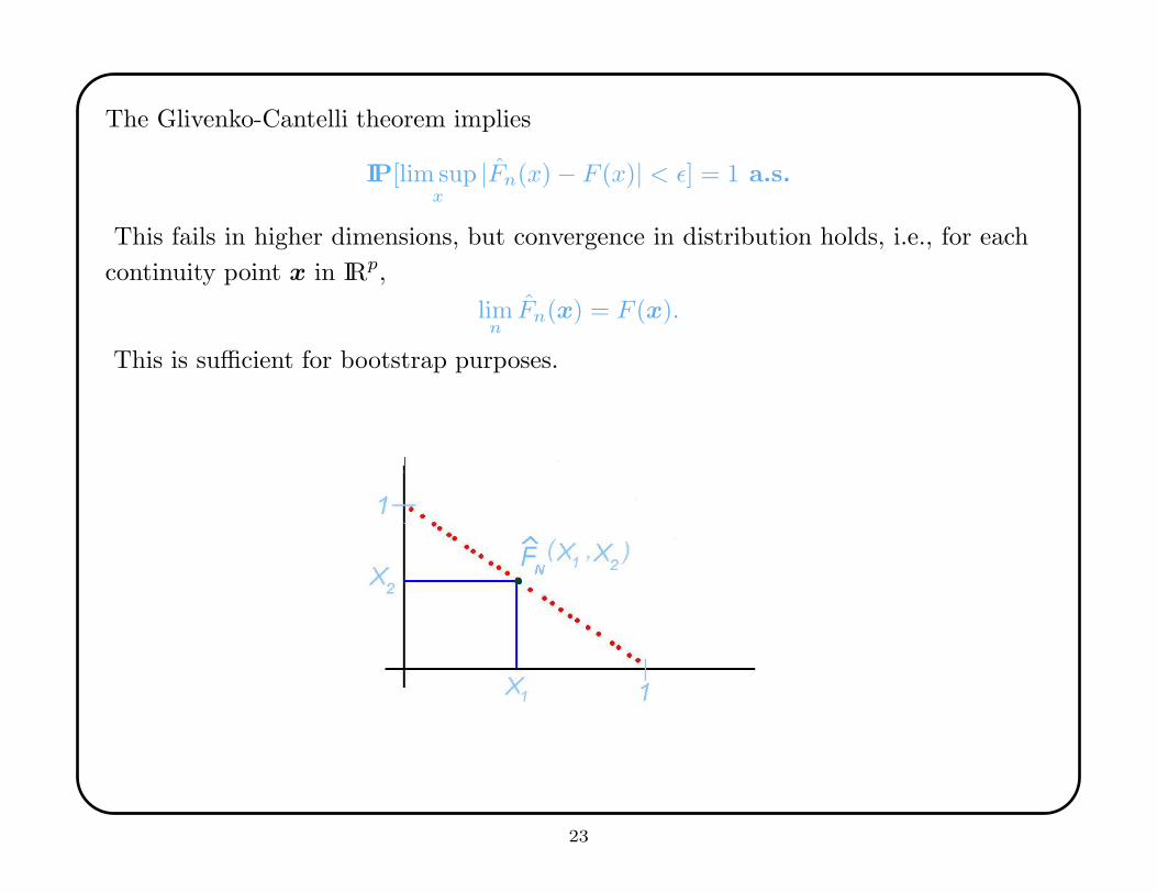
The Glivenko-Cantelli theorem implies
IP[lim supx
|Fn(x) − F (x)| < ε] = 1 a.s.
This fails in higher dimensions, but convergence in distribution holds, i.e., for each
continuity point x in IRp,
limnFn(x) = F (x).
This is sufficient for bootstrap purposes.
23
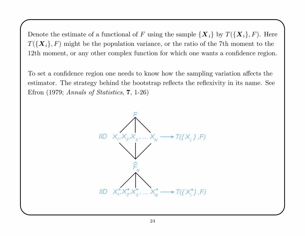
Denote the estimate of a functional of F using the sample {X i} by T ({Xi}, F ). Here
T ({Xi}, F ) might be the population variance, or the ratio of the 7th moment to the
12th moment, or any other complex function for which one wants a confidence region.
To set a confidence region one needs to know how the sampling variation affects the
estimator. The strategy behind the bootstrap reflects the reflexivity in its name. See
Efron (1979; Annals of Statistics, 7, 1-26)
24
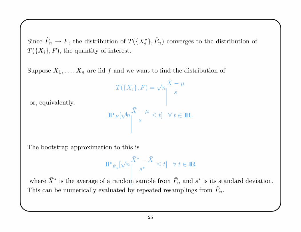
Since Fn → F , the distribution of T ({X∗i }, Fn) converges to the distribution of
T ({Xi}, F ), the quantity of interest.
Suppose X1, . . . , Xn are iid f and we want to find the distribution of
T ({Xi}, F ) =√nX − µ
s
or, equivalently,
IPF [√nX − µ
s≤ t] ∀ t ∈ IR.
The bootstrap approximation to this is
IPFn[√nX∗ − X
s∗≤ t] ∀ t ∈ IR
where X∗ is the average of a random sample from Fn and s∗ is its standard deviation.
This can be numerically evaluated by repeated resamplings from Fn.
25
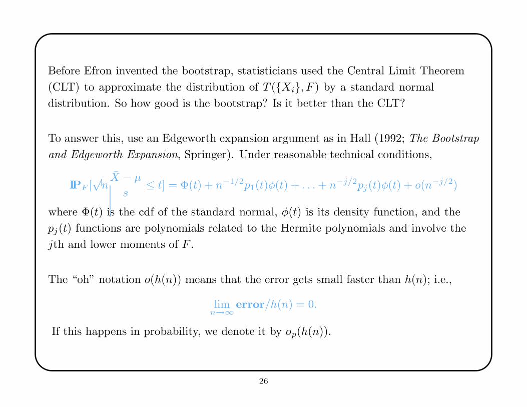
Before Efron invented the bootstrap, statisticians used the Central Limit Theorem
(CLT) to approximate the distribution of T ({Xi}, F ) by a standard normal
distribution. So how good is the bootstrap? Is it better than the CLT?
To answer this, use an Edgeworth expansion argument as in Hall (1992; The Bootstrap
and Edgeworth Expansion, Springer). Under reasonable technical conditions,
IPF [√nX − µ
s≤ t] = Φ(t) + n−1/2p1(t)φ(t) + . . .+ n−j/2pj(t)φ(t) + o(n−j/2)
where Φ(t) is the cdf of the standard normal, φ(t) is its density function, and the
pj(t) functions are polynomials related to the Hermite polynomials and involve the
jth and lower moments of F .
The “oh” notation o(h(n)) means that the error gets small faster than h(n); i.e.,
limn→∞
error/h(n) = 0.
If this happens in probability, we denote it by op(h(n)).
26
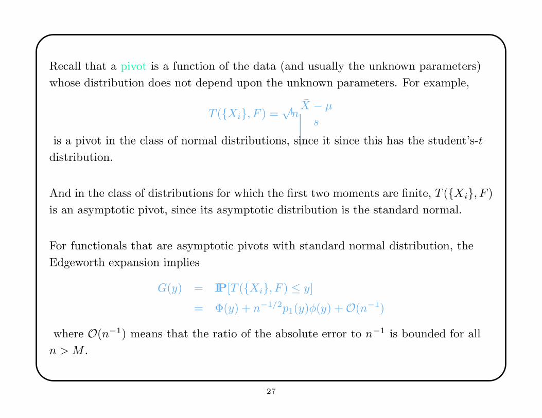
Recall that a pivot is a function of the data (and usually the unknown parameters)
whose distribution does not depend upon the unknown parameters. For example,
T ({Xi}, F ) =√nX − µ
s
is a pivot in the class of normal distributions, since it since this has the student’s-t
distribution.
And in the class of distributions for which the first two moments are finite, T ({Xi}, F )
is an asymptotic pivot, since its asymptotic distribution is the standard normal.
For functionals that are asymptotic pivots with standard normal distribution, the
Edgeworth expansion implies
G(y) = IP[T ({Xi}, F ) ≤ y]
= Φ(y) + n−1/2p1(y)φ(y) + O(n−1)
where O(n−1) means that the ratio of the absolute error to n−1 is bounded for all
n > M .
27
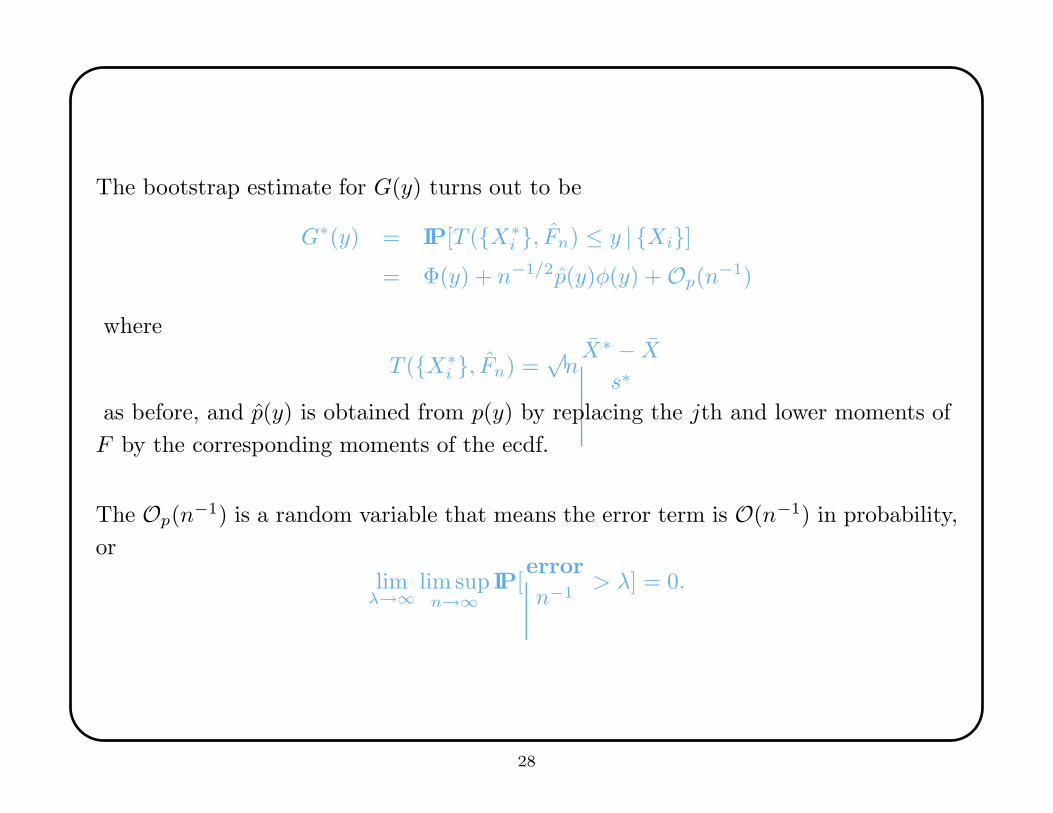
The bootstrap estimate for G(y) turns out to be
G∗(y) = IP[T ({X∗i }, Fn) ≤ y | {Xi}]
= Φ(y) + n−1/2p(y)φ(y) + Op(n−1)
where
T ({X∗i }, Fn) =
√nX∗ − X
s∗
as before, and p(y) is obtained from p(y) by replacing the jth and lower moments of
F by the corresponding moments of the ecdf.
The Op(n−1) is a random variable that means the error term is O(n−1) in probability,
or
limλ→∞
lim supn→∞
IP[error
n−1> λ] = 0.
28
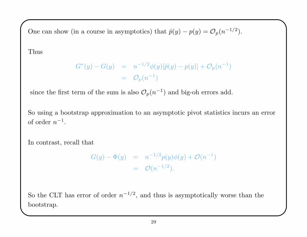
One can show (in a course in asymptotics) that p(y) − p(y) = Op(n−1/2).
Thus
G∗(y) −G(y) = n−1/2φ(y)[p(y) − p(y)] + Op(n−1)
= Op(n−1)
since the first term of the sum is also Op(n−1) and big-oh errors add.
So using a bootstrap approximation to an asymptotic pivot statistics incurs an error
of order n−1.
In contrast, recall that
G(y) − Φ(y) = n−1/2p(y)φ(y) + O(n−1)
= O(n−1/2).
So the CLT has error of order n−1/2, and thus is asymptotically worse than the
bootstrap.
29
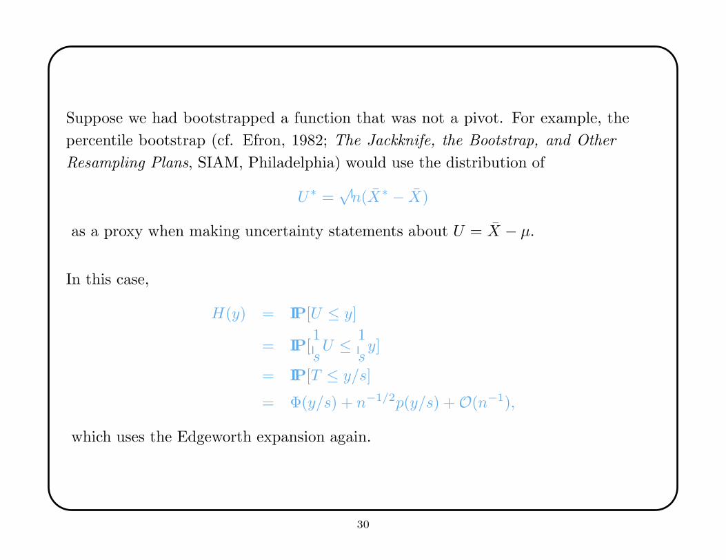
Suppose we had bootstrapped a function that was not a pivot. For example, the
percentile bootstrap (cf. Efron, 1982; The Jackknife, the Bootstrap, and Other
Resampling Plans, SIAM, Philadelphia) would use the distribution of
U∗ =√n(X∗ − X)
as a proxy when making uncertainty statements about U = X − µ.
In this case,
H(y) = IP[U ≤ y]
= IP[1
sU ≤ 1
sy]
= IP[T ≤ y/s]
= Φ(y/s) + n−1/2p(y/s) + O(n−1),
which uses the Edgeworth expansion again.
30
Similarly,
H∗(y) = IP[U∗ ≤ y | {XI}]= Φ(y/s∗) + n−1/2p(y/s∗)φ(y/s∗) + O(n−1).
From asymptotics, it can be shown that:
p(y/s) − p(y/s∗) = Op(n−1/2)
s− s∗ = Op(n−1/2).
Thus
H(y)−H∗(y) = Φ(y/s)−Φ(y/s∗) + n−1/2[p(y/s)φ(y/s)− p(y/s∗)φ(y/s∗)] +Op(n−1).
The second term has order Op(n−1) but the first has order Op(n
−1/2).
So when the statistic is not an asymptotic pivot, the bootstrap and the CLT have the
same asymptotics. It pays to bootstrap a studentized pivot.
31
2. Smoothing
A smoothing algorithm is a summary of trend in Y as a function of explanatory
variables X1, . . . , Xp. The smoother takes data and returns a function, called a
smooth.
We focus on scatterplot smooths, for which p = 1. These usually generalize to p = 2
and p = 3, but the COD quickly renders them impractical. Even so, they can be used
as building blocks for more sophisticated smoothing algorithms that break down less
badly with large p, and we discuss several standard smoothers it illustrate the issues
and tradeoffs.
Essentially, a smooth just finds an estimate of f in the nonparametric regression
function Y = f(x) + ε.
32
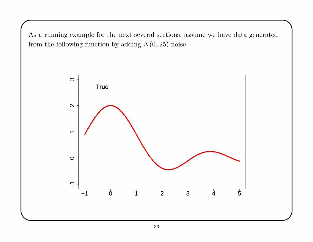
As a running example for the next several sections, assume we have data generated
from the following function by adding N(0..25) noise.
−1 0 1 2 3 4 5
−1
01
23
True
33
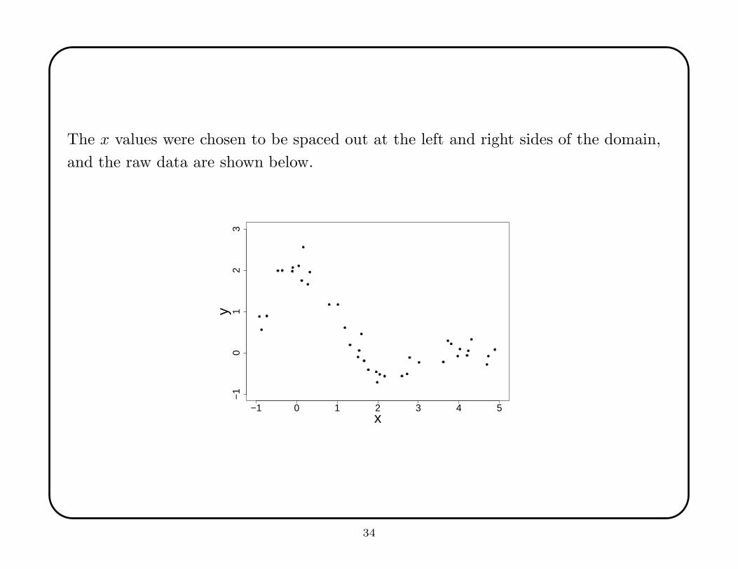
The x values were chosen to be spaced out at the left and right sides of the domain,
and the raw data are shown below.
−1 0 1 2 3 4 5
−1
01
23
x
y
34
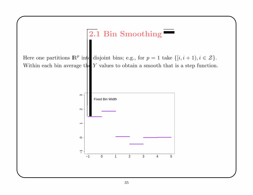
2.1 Bin Smoothing
Here one partitions IRp into disjoint bins; e.g., for p = 1 take {[i, i + 1), i ∈ Z}.Within each bin average the Y values to obtain a smooth that is a step function.
−1 0 1 2 3 4 5
−1
01
23
Fixed Bin Width
35
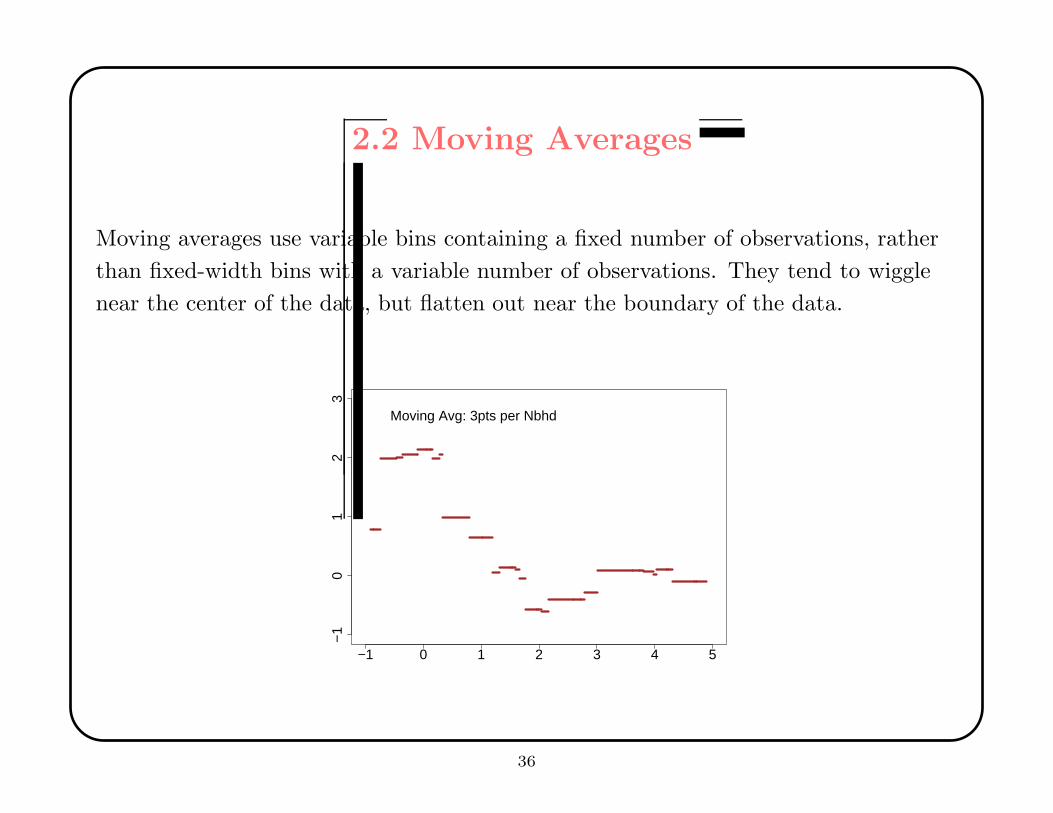
2.2 Moving Averages
Moving averages use variable bins containing a fixed number of observations, rather
than fixed-width bins with a variable number of observations. They tend to wiggle
near the center of the data, but flatten out near the boundary of the data.
−1 0 1 2 3 4 5
−1
01
23
Moving Avg: 3pts per Nbhd
36
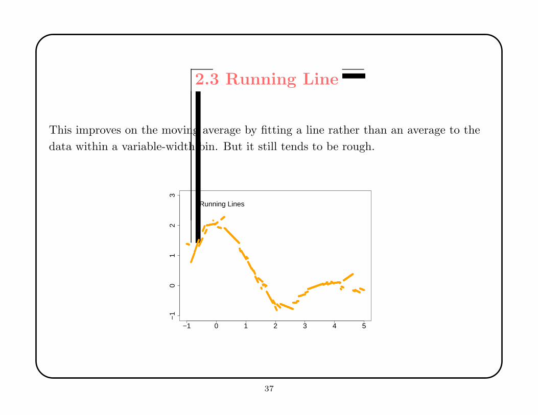
2.3 Running Line
This improves on the moving average by fitting a line rather than an average to the
data within a variable-width bin. But it still tends to be rough.
−1 0 1 2 3 4 5
−1
01
23
Running Lines
37
2.4 Loess
Loess was developed by Cleveland (1979; Journal of the American Statistical
Association, 84, 829-836).
Loess extends the running line smooth by using weighted linear regression inside
the variable-width bins. Loess is more computationally intensive, but is often
satisfactorily smooth and flexible.
LOESS fits the model
IE[Y ] = θ(x)′x
where
θ(x) = argminθ∈IRp
n∑
i=1
wi(x)(Yi − θ′Xi)2
and wi is a weight function that governs the influence of the ith datum according to
the direction and distance of X i from x.
38
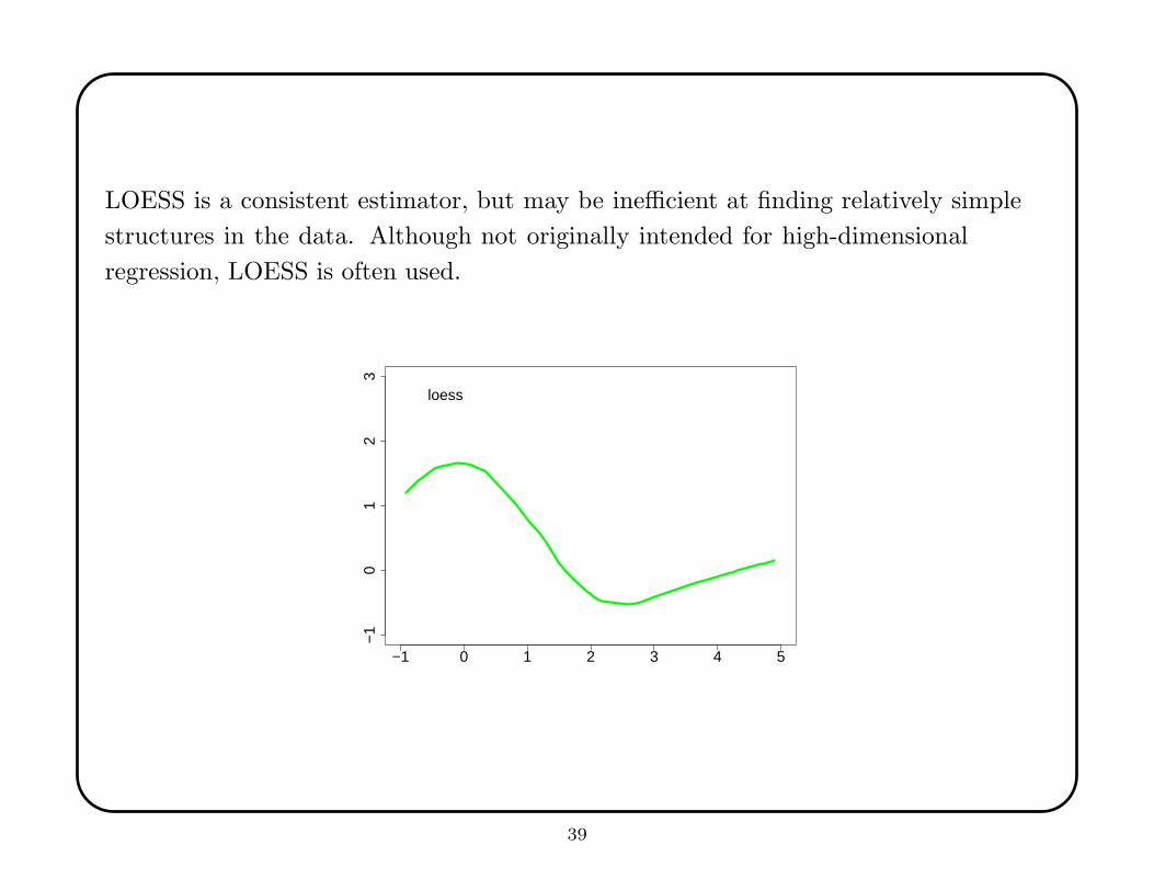
LOESS is a consistent estimator, but may be inefficient at finding relatively simple
structures in the data. Although not originally intended for high-dimensional
regression, LOESS is often used.
−1 0 1 2 3 4 5
−1
01
23
loess
39

2.5 Kernel Smoothers
These are much like moving averages except that the average is weighted and the
bin-width is fixed. Kernel smoothers work well and are mathematically tractable. The
weights in the average depend upon the kernel K(x). A kernel is usually symmetric,
continuous, nonnegative, and integrates to 1 (e.g., a Gaussian kernel).
The bin-width is set by h, also called the bandwidth. This can vary, adapting to
information in the data on the roughness of the function.
Let {(yi,xi)} denote the sample. Set Kh(x) = h−1K(h−1x). Then the
Nadaraya-Watson estimate of f at x is
f(x) =
∑ni=1 Kh(x − xi)yi∑n
i=1 Kh(x − xi).
See Watson (1964; Theory and Probability Applications, 10, 186-190) and Nadaraya
(1964; Sankha A, 26, 359-372).
40
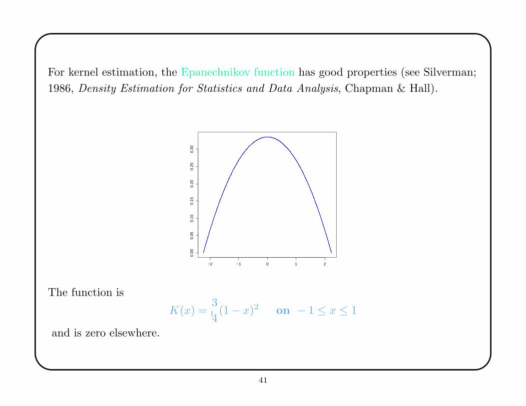
For kernel estimation, the Epanechnikov function has good properties (see Silverman;
1986, Density Estimation for Statistics and Data Analysis, Chapman & Hall).
−2 −1 0 1 2
0.00
0.05
0.10
0.15
0.20
0.25
0.30
The function is
K(x) =3
4(1 − x)2 on − 1 ≤ x ≤ 1
and is zero elsewhere.
41

Intentional blank.
42
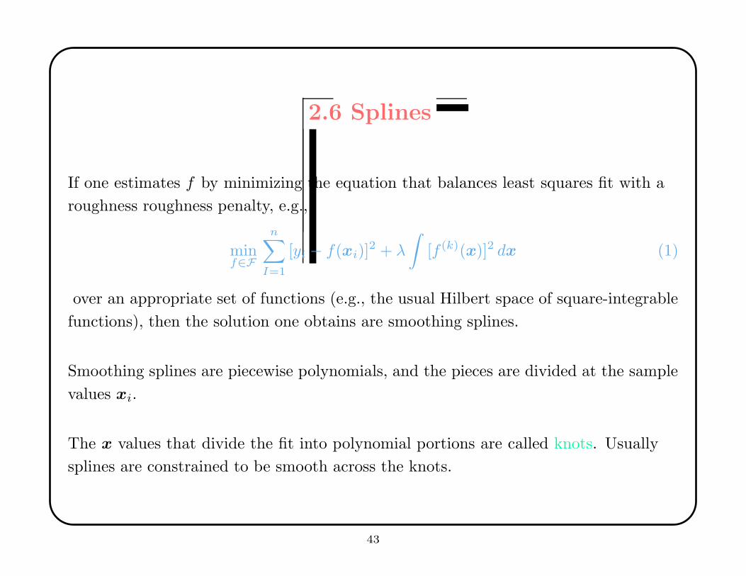
2.6 Splines
If one estimates f by minimizing the equation that balances least squares fit with a
roughness roughness penalty, e.g.,
minf∈F
n∑
I=1
[yi − f(xi)]2 + λ
∫
[f (k)(x)]2 dx (1)
over an appropriate set of functions (e.g., the usual Hilbert space of square-integrable
functions), then the solution one obtains are smoothing splines.
Smoothing splines are piecewise polynomials, and the pieces are divided at the sample
values xi.
The x values that divide the fit into polynomial portions are called knots. Usually
splines are constrained to be smooth across the knots.
43

intentional blank
44

intentional blank
45

Regression splines have fixed knots that need not depend upon the data. Also, knot
selection techniques enable one to find good knots automatically.
Splines are computationally fast, enjoy strong theory, work well, and are widely used.
−1 0 1 2 3 4 5
−1
01
23
Spline
46
2.7 Comparing Smoothers
Most smoothing methods are approximately kernel smoothers, with parameters that
correspond to the kernel K(x) and the bandwidth h.
In practice, one can:
• fix h by judgment,
• find the optimal fixed h,
• fit h adaptively from the data,
• fit the kernel K(x) adaptively from the data.
There is a point of diminishing returns, and this is usually hit when one fits the h
adaptively.
Scott (1992; Multivariate Density Estimation, Wiley) provides a nice discussion of
smoothing issues in the context of density estimation.
47
Breiman and Peters (1992; International Statistics Review, 60, 271-290) give results
on a simulation experiment to compare smoothers. Broadly, they found that:
• adaptive kernel smoothing is good but slow,
• smoothing splines are accurate but too rough in large samples,
• everything else is not really competitive in hard problems (i.e., those with large
sample sizes and/or high dimensions).
Theoretical understanding of the properties of smoothing depends upon the
eigenstructure of the smoothing matrix. Hastie, Tibshirani, and Freidman (2001; The
Elements of Statistical Learning, Springer) provide an introduction and summary of
this area in Chapter 5.
48
In linear regression one starts with a quantity of information equal to n degrees of
freedom where n is the number of independent observations in the sample. Each
estimated parameter reduces the information by 1 degree of freedom. This Occurs
because each estimate corresponds to a linear constraint in IRn, the space in which
the n observations lie.
Smoothing is a nonlinear constraint and costs more information. But most smoothers
can be expressed as a linear operator (matrix) S acting on the response vector
y ∈ IRn. It turns out that the degrees of freedom lost to smoothing is then tr(S).
Most smoothers are shrinkage estimators. Mathematically, they pull the weights on
the coefficients in the basis expansion for y towards zero.
Shrinkage is why smoothing has an effective degrees of freedom between p (as in
regression, which does not shrink) and n (which is what one would expect from a
naive count of the number of parameters).
49
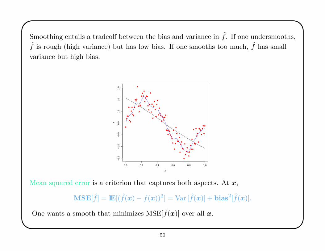
Smoothing entails a tradeoff between the bias and variance in f . If one undersmooths,
f is rough (high variance) but has low bias. If one smooths too much, f has small
variance but high bias.
0.0 0.2 0.4 0.6 0.8 1.0
−1.
5−
1.0
−0.
50.
00.
51.
01.
5
x
y
Mean squared error is a criterion that captures both aspects. At x,
MSE[f ] = IE[(f(x) − f(x))2] = Var [f(x)] + bias2[f(x)].
One wants a smooth that minimizes MSE[f(x)] over all x.
50

intentional blank
51

intentional blank
52

3. Search and Variable Selection
Data mining entails many kinds of search. Some searches are easier than others.
A relatively easy kind of search is univariate. For example, one might want to find
an appropriate bandwidth h for a smoother or the appropriate degree for fitting a
polynomial regression or the number of terms to include in a model.
Search becomes harder in multivariate cases, such as finding an appropriate set of
knots for spline smoothing or a set of weights in a neural network.
Even more difficult is combinatorial search, where there is no natural Euclidean space.
This occurs in variable selection (a/k/a feature selection).
The hardest search is list search, where there is no structure in the problem at all.
This occurs, for example, when there is a list of possible models, each of which is
largely unrelated to the others, and one wants to find the best model for the data.
53
3.1 Univariate Search
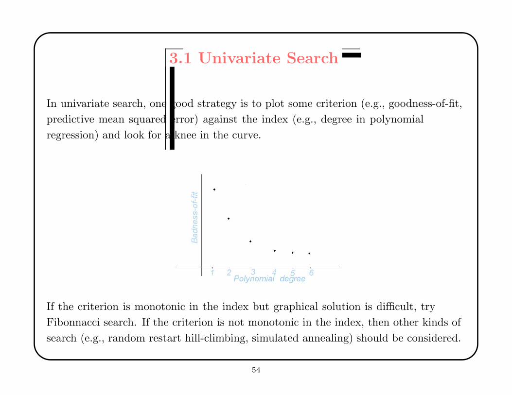
In univariate search, one good strategy is to plot some criterion (e.g., goodness-of-fit,
predictive mean squared error) against the index (e.g., degree in polynomial
regression) and look for a knee in the curve.
If the criterion is monotonic in the index but graphical solution is difficult, try
Fibonnacci search. If the criterion is not monotonic in the index, then other kinds of
search (e.g., random restart hill-climbing, simulated annealing) should be considered.
54

intentional blank
55
3.2 Multivariate Search
For multivariate search, there are dozens of smart algorithms, and the best choice
depends upon the nature of the response surface.
If the surface has a single bump, then steepest ascent works very well. If the surface
has many bumps, then random restart combined with steepest ascent is a strategy
that enables one to make probability statements about the chance that one has found
a global maximum.
The Nelder-Mead algorithm is simple to program and very robust. It sets a simplex
in the space IRk and passes the worst vertex through the center to the opposite side.
(Nelder and Mead; 1965, Computer Journal, 7, 308-313.)
Hybrid methods combine features from standard operations research algorithms and
allow one to learn about the surface as one seeks the maximum.
56
3.3 Variable Selection
For combinatorial search, one wants to take advantage of whatever structure the
problem enjoys.
For example, variable selection is a key problem in data mining. Often one has very
large p and one wants (needs) to discard those that have no or little predictive value.
If one looked at all possible subsets of variables, there are 2p cases to consider.
Something smarter is needed.
The 2p possible models can be identified with the 2p vertices of the unit hypercube in
IRp. The (0, 0, . . . , 0) vertex corresponds to the model with all variables excluded,
whereas the (1, 1, . . . , 1) model is the regression on all variables. From this
perspective, a clever search of the hypercube would be an attractive way to find a
good regression model.
57
3.3.1 Gray Codes
A Hamiltonian circuit of the unit hypercube is a traversal that reaches each vertex
exactly once. There are many possible Hamiltonian circuits—the exact number is not
known.
From the standpoint of model search, one wants a Hamiltonian circuit that has
desirable properties of symmetry, treating all vertices in the same way.
The Gray code is a procedure for listing the vertices of the hypercube in such a way
that there is no repetition, each vertex is one edge from the previous vertex, and all
vertices in a neighborhood are explored before moving on to a new neighborhood.
Wilf (1989; Combinatorial Algorithms: An Update, SIAM) describes the mathematical
theory and properties of the Gray code system.
58
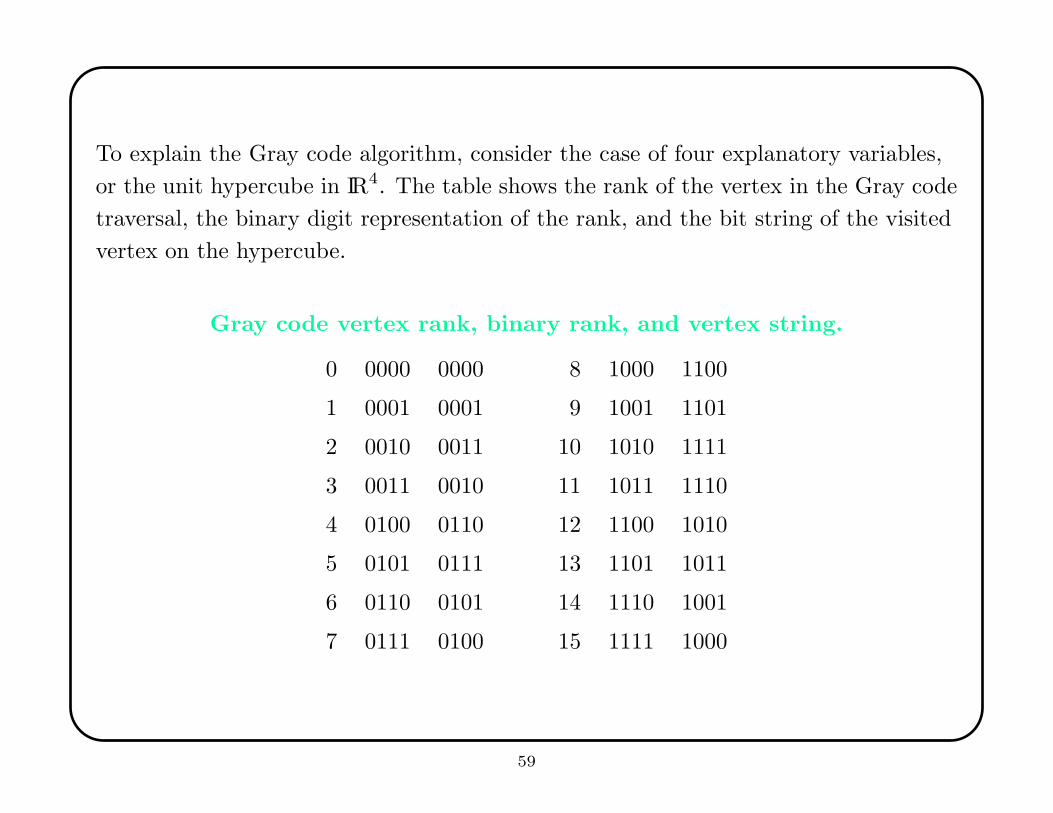
To explain the Gray code algorithm, consider the case of four explanatory variables,
or the unit hypercube in IR4. The table shows the rank of the vertex in the Gray code
traversal, the binary digit representation of the rank, and the bit string of the visited
vertex on the hypercube.
Gray code vertex rank, binary rank, and vertex string.
0 0000 0000 8 1000 1100
1 0001 0001 9 1001 1101
2 0010 0011 10 1010 1111
3 0011 0010 11 1011 1110
4 0100 0110 12 1100 1010
5 0101 0111 13 1101 1011
6 0110 0101 14 1110 1001
7 0111 0100 15 1111 1000
59
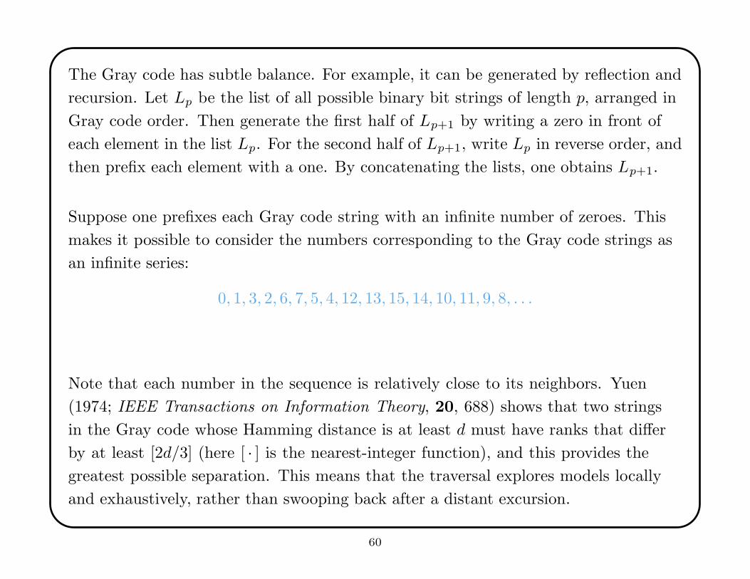
The Gray code has subtle balance. For example, it can be generated by reflection and
recursion. Let Lp be the list of all possible binary bit strings of length p, arranged in
Gray code order. Then generate the first half of Lp+1 by writing a zero in front of
each element in the list Lp. For the second half of Lp+1, write Lp in reverse order, and
then prefix each element with a one. By concatenating the lists, one obtains Lp+1.
Suppose one prefixes each Gray code string with an infinite number of zeroes. This
makes it possible to consider the numbers corresponding to the Gray code strings as
an infinite series:
0, 1, 3, 2, 6, 7, 5, 4, 12, 13, 15, 14, 10, 11, 9, 8, . . .
Note that each number in the sequence is relatively close to its neighbors. Yuen
(1974; IEEE Transactions on Information Theory, 20, 688) shows that two strings
in the Gray code whose Hamming distance is at least d must have ranks that differ
by at least [2d/3] (here [ · ] is the nearest-integer function), and this provides the
greatest possible separation. This means that the traversal explores models locally
and exhaustively, rather than swooping back after a distant excursion.
60
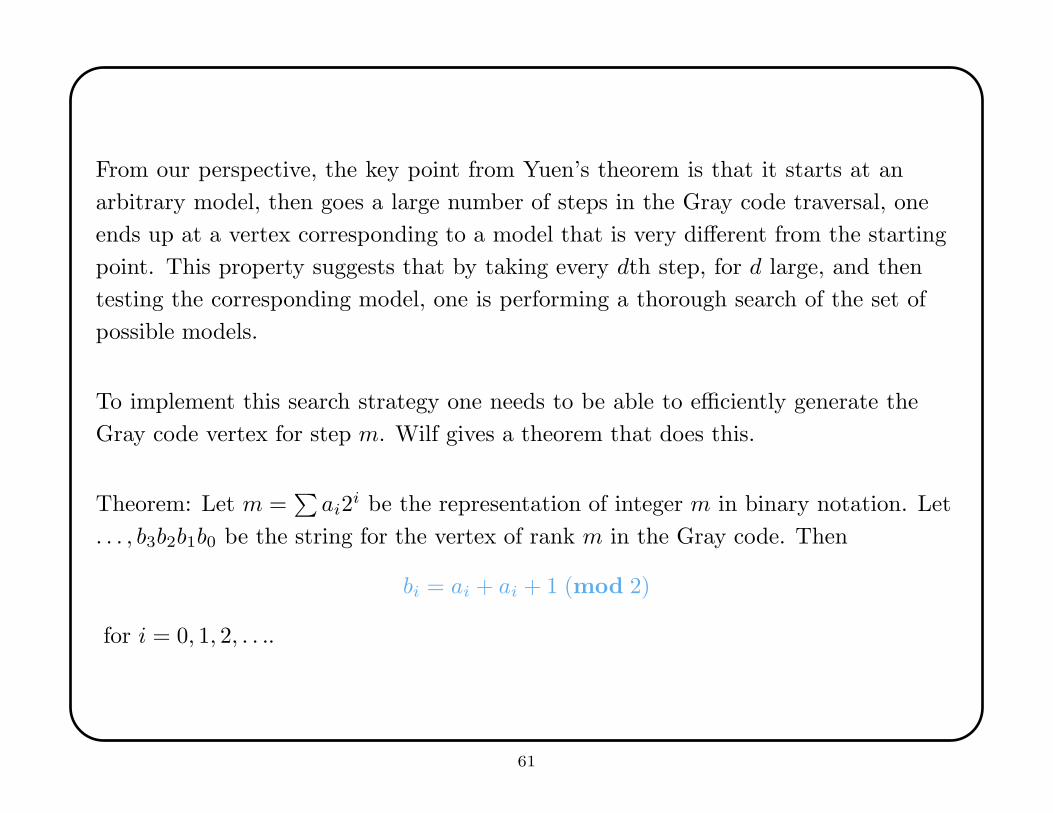
From our perspective, the key point from Yuen’s theorem is that it starts at an
arbitrary model, then goes a large number of steps in the Gray code traversal, one
ends up at a vertex corresponding to a model that is very different from the starting
point. This property suggests that by taking every dth step, for d large, and then
testing the corresponding model, one is performing a thorough search of the set of
possible models.
To implement this search strategy one needs to be able to efficiently generate the
Gray code vertex for step m. Wilf gives a theorem that does this.
Theorem: Let m =∑
ai2i be the representation of integer m in binary notation. Let
. . . , b3b2b1b0 be the string for the vertex of rank m in the Gray code. Then
bi = ai + ai + 1 (mod 2)
for i = 0, 1, 2, . . ..
61
To use this ranking theorem to efficiently explore a set of models, suppose one decides
to examine only 100 models and then infer the final fit.
If there are p explanatory variables, one takes d = [2p/100], and then finds the Gray
code vertex sequences of rank d, 2d, . . . , 100d.
Each sequence defines a particular set of variables that may be included or excluded
in the regression. In practice, one would examine the 100 model fitting results,
probably in terms of the square root of the adjusted R2, and then home in on the
region of the cube that provides good explanation.
This enables one to quickly identify the vertex or bit string corresponding to a set
of variables that provides good explanation. One might make additional Gray code
searches in the region of the best results from the first search, and iterate to find the
final model.
62

3.3.3 Experimental Design Selection
Another approach to variable selection uses ideas from experimental design. The
method is due to Clyde (1999; Bayesian Statistics 6, 157-185, Oxford University
Press).
To implement this approach, one views each explanatory variable as a factor in an
experimental design. All factors have two levels, corresponding to whether or not the
explanatory variable is included in the model. This enables one to perform a 2p−k
fractional factorial experiment in which one fits a multiple regression model to the
included variables and records some measure of goodness-of-fit.
Obviously, one takes k to be sufficiently large that it is possible to perform the
computations in a reasonable amount of time and also to limit the effect of multiple
testing.
63
One uses analysis of variance to examine which factors and factor combinations
have a significant influence on the observations. Significant main effects correspond
to explanatory variables that contribute on their own. Significant interaction terms
correspond to subsets of variables whose joint inclusion in the model provides
explanation.
In multiple linear regression, these results are implicit in significance tests on the
coefficients. But if one using one of the nonparametric regression techniques popular
in data mining (e.g., MARS, PPR, neural nets), this helps find influential variables.
Based on the results of the designed experiment, one can ultimately find and fit
the model that includes all variables corresponding to significant main effects or
interactions. And the factorial design reduces the penalty one pays for multiple
testing, as compared to exhaustive search or other less-efficient searches.
64
Possible measures of goodness-of-fit include:
• R2, the proportion of variance in the observations that is explained by the model;
• Adjusted R2, the proportion of variance in the observations that is explained by
the model, but with an adjustment to account for the number of variables in the
model;
• Mallows’ Cp, a measure of predictive accuracy that takes account of the number
of terms in the model.
• MISE, the mean integrated squared error of the fitted model over a given region
(often the hyperrectangle defined by the minimum and maximum values taken by
each explanatory variable used in the model.
• The square root of the adjusted R2, since this transformation appears to stabilize
the variance and thereby supports use of analysis of variance and response surface
methodology in the model search.
Weisberg (1985, Applied Linear Regression, 185-190, Wiley) discusses the first three.
Scott (1992, Multivariate Density Estimation, chapter 2.4, Wiley) discusses MISE.
65

3.4 List Search
With list search, there is no exploitable structure that links the elements of the list,
and the list is usually so long that exhaustive search is infeasible.
There is not much that one can do. If one tests entries on the list at random, then
one can try some of the following:
• Estimate the proportion of list entries that give results above some threshold.
• Use some modeling to estimate the maximum value on the list from a random
sample of list entries.
• Estimate the probability that further search will discover a new maximum within
a fixed amount of time.
• Use the solution to the Secretary Problem.
66
A strategy invented by computer scientists (Maron and Moore, 1997, Artificial
Intelligence Review, 11 193-225) is to race the testing.
One does pairwise comparisons of models. At first, one fits only a small random
fraction of the data (say a random 1%) to each model on the list. Usually this is
sufficient to discover which model is best and one discards the other.
If that small fraction does not distinguish the models, then one fits another small
fraction. Only very rarely is it necessary to fit all or most of the data to select the
better model.
Racing is an easy way to extend one’s search capability by about 100-fold.
67
4. Nonparametric Regression
The multiple linear regression model is
Y = β0 + β1X1 + . . .+ βpXp + ε
where IE[ε] = 0, Var [ε] = σ2, and ε is independent of x1, . . . , xp.
The model is useful because:
• it is interpretable—the effect of each explanatory variable is captured by a single
coefficient
• theory supports inference and prediction is easy
• simple interactions and transformations are easy
• dummy variables allow use of categorical information
• computation is fast.
68
4.1 Additive Models
But additive linear fits are too flat. And the class of all possible smooths is too
large—the COD makes it hard to smooth in high dimensions. The class of additive
models is a useful compromise.
The additive model is
Y = β0 +
p∑
k=1
fk(xk) + ε
where the fk are unknown smooth functions fit from the data.
The basic assumptions are as before, except we must add IE[fk(Xk)] = 0 in order to
prevent identifiability problems.
The parameters in the additive model are {fk}, β0, and σ2. In the linear model, each
parameter that is fit costs one degree of freedom, but fitting the functions costs more,
depending upon what kind of univariate smoother is used.
69

Some notes:
• one can require that some of the fk be linear or monotone;
• one can include some low-dimensional smooths, such as f(X1, X2);
• one can include some kinds of interactions, such as f(X1X2);
• transformation of variables is done automatically;
• many regression diagnostics, such as Cook’s distance, generalize to additive
models;
• ideas from weighted regression generalize to handle heteroscedasticity;
• approximate deviance tests for comparing nested additive models are available;
• one can use the bootstrap to set pointwise confidence bands on the fk (if these
include the zero function, omit the term);
However, model selection, overfitting, and multicollinearity (concurvity) are serious
problems. And the final fit may still be poor.
70
4.1.1 The Backfitting Algorithm
The backfitting algorithm is used to fit additive models. It allows one to use an
arbitrary smoother (e.g., spline, Loess, kernel) to estimate the {fk}
As motivation, suppose that the additive model is exactly correct. The for all
k = 1, . . . , p,
IE[Y − β0 −∑
k 6=j
fk(Xk) |xj ] = fj(xj).
The backfitting algorithm solves these p estimating equations iteratively. At
each stage it replaces the conditional expectation of the partial residuals, i.e.,
Y − β0 −∑
k 6=j fk(Xk) with a univariate smooth.
Notation: Let y be the vector of responses, let X be the n× p matrix of explanatory
values with columns x·k. Let fk be the vector whose ith entry is fk(xik) for
i = 1, . . . , n.
71
For z ∈ IRn, let S(z |x·k) be a smooth of the scatterplot of z against the values of the
kth explanatory variable.
The backfitting algorithm works as follows:
1. Initialize. Set β0 = Y and set the fk functions to be something reasonable (e.g., a
linear regression). Set the fk vectors to match.
2. Cycle. For j = 1, . . . , p set
fk = S(Y − β0 −∑
k 6=j
fk |x·k)
and update the fk to match.
3. Iterate. Repeat step (2) until the changes in the fk between iterations is
sufficiently small.
One may use different smoothers for different variables, or bivariate smoothers for
predesignated pairs of explanatory variables.
72
The estimating equations that are the basis for the backfitting algorithm have the
form:
Pf = QY
for suitable matrices P and Q.
The iterative solution for this has the structure of a Gauss-Seidel algorithm for linear
systems (cf. Hastie and Tibshirani; 1990, Generalized Additive Models, chap. 5.2).
This structure ensures that the backfitting algorithm converges for smoothers that
correspond to a symmetric smoothing matrix with all eigenvalues in (0, 1). This
includes smoothing splines and most kernel smoothers, but not Loess.
If it converges, the solution is unique unless there is concurvity. In that case, the
solution depends upon the initial conditions.
73
Concurvity occurs when the {xi} values lie upon a smooth manifold in IRp. In our
context, a manifold is smooth if the smoother used in backfitting can interpolate all
the {xi} perfectly.
This is exactly analogous to the non-uniqueness of regression solutions when the X
matrix is not full-rank.
Let P be an operator on p-tuples of functions g = (g1, . . . , gp) and let Q be an
operator on a function h. Then the concurvity space of
Pg = Qh
is the set of additive functions g(x) =∑
gj(xj) such that Pg = 0. That is,
gj(xj) + IE[∑
k 6=j
gk(xk) |xj ] = 0.
We shall now consider several extensions of the general idea in additive modeling.
74
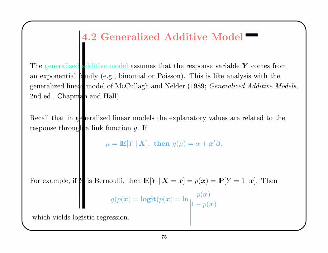
4.2 Generalized Additive Model
The generalized additive model assumes that the response variable Y comes from
an exponential family (e.g., binomial or Poisson). This is like analysis with the
generalized linear model of McCullagh and Nelder (1989; Generalized Additive Models,
2nd ed., Chapman and Hall).
Recall that in generalized linear models the explanatory values are related to the
response through a link function g. If
µ = IE[Y |X], then g(µ) = α+ x′β.
For example, if Y is Bernoulli, then IE[Y |X = x] = p(x) = IP[Y = 1 |x]. Then
g(p(x) = logit(p(x) = lnp(x)
1 − p(x)
which yields logistic regression.
75
The generalized additive model expresses the link function as an additive, rather than
linear, function of x:
g(µ) = β0 +
p∑
j=1
fj(xj).
As before, the link function is chosen by the user based on domain knowledge. Only
the relation to the explanatory variables is modeled.
Thus an additive model version of logistic regression is
logit(p(x)) = β0 +
p∑
j=1
fj(xj).
Generalized linear models are fit by iterative scoring, a form of iteratively reweighted
least squares. The generalized additive model modifies backfitting in a similar way
(cf. Hastie and Tibshirani; 1990, Generalized Additive Models, chap. 6).
76

intentional blank
77
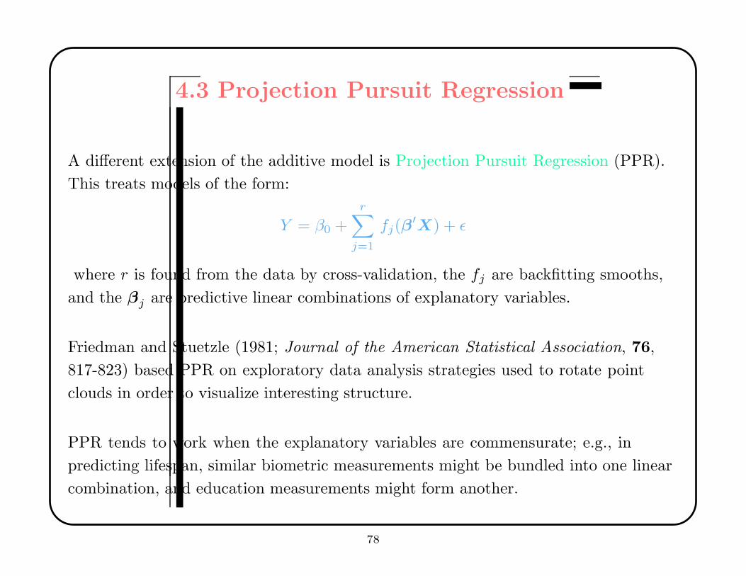
4.3 Projection Pursuit Regression
A different extension of the additive model is Projection Pursuit Regression (PPR).
This treats models of the form:
Y = β0 +r∑
j=1
fj(β′X) + ε
where r is found from the data by cross-validation, the fj are backfitting smooths,
and the βj are predictive linear combinations of explanatory variables.
Friedman and Stuetzle (1981; Journal of the American Statistical Association, 76,
817-823) based PPR on exploratory data analysis strategies used to rotate point
clouds in order to visualize interesting structure.
PPR tends to work when the explanatory variables are commensurate; e.g., in
predicting lifespan, similar biometric measurements might be bundled into one linear
combination, and education measurements might form another.
78
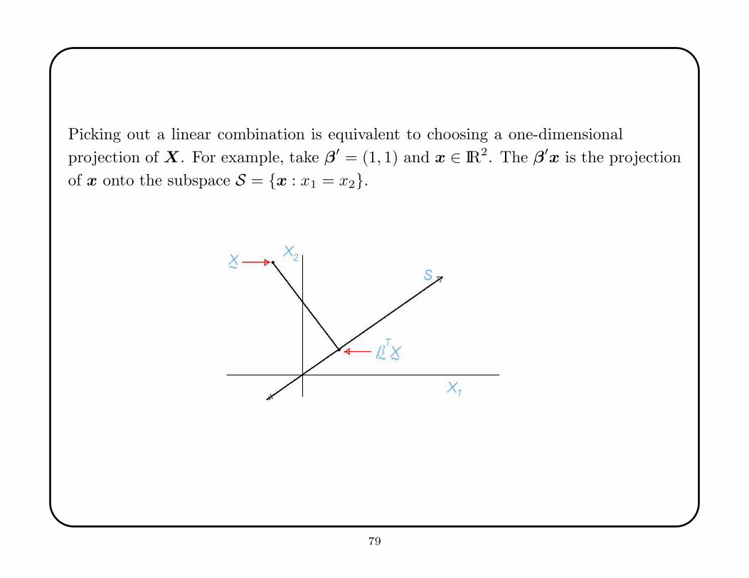
Picking out a linear combination is equivalent to choosing a one-dimensional
projection of X. For example, take β′ = (1, 1) and x ∈ IR2. The β′x is the projection
of x onto the subspace S = {x : x1 = x2}.
79
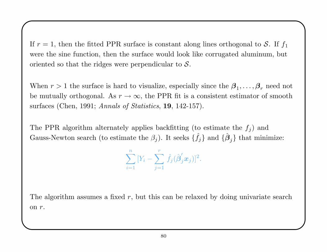
If r = 1, then the fitted PPR surface is constant along lines orthogonal to S. If f1
were the sine function, then the surface would look like corrugated aluminum, but
oriented so that the ridges were perpendicular to S.
When r > 1 the surface is hard to visualize, especially since the β1, . . . ,βr need not
be mutually orthogonal. As r → ∞, the PPR fit is a consistent estimator of smooth
surfaces (Chen, 1991; Annals of Statistics, 19, 142-157).
The PPR algorithm alternately applies backfitting (to estimate the fj) and
Gauss-Newton search (to estimate the βj). It seeks {fj} and {βj} that minimize:
n∑
i=1
[Yi −r∑
j=1
fj(β′jxj)]
2.
The algorithm assumes a fixed r, but this can be relaxed by doing univariate search
on r.
80
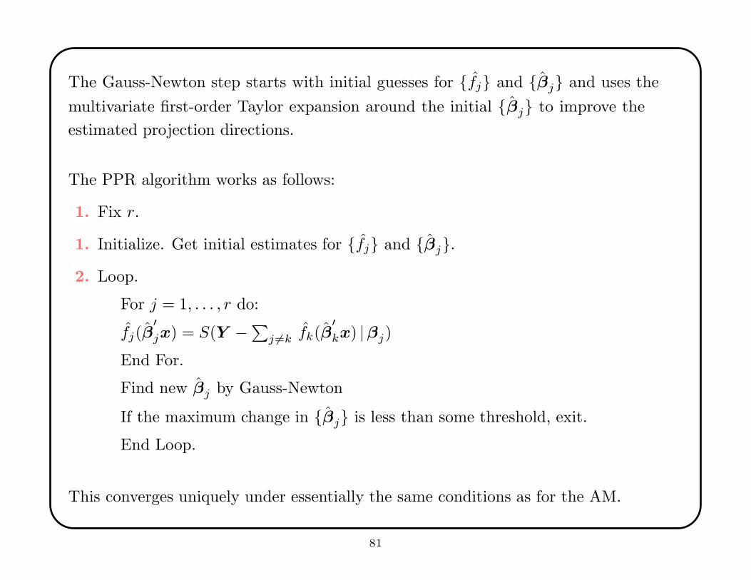
The Gauss-Newton step starts with initial guesses for {fj} and {βj} and uses the
multivariate first-order Taylor expansion around the initial {βj} to improve the
estimated projection directions.
The PPR algorithm works as follows:
1. Fix r.
1. Initialize. Get initial estimates for {fj} and {βj}.
2. Loop.
For j = 1, . . . , r do:
fj(β′jx) = S(Y −∑j 6=k fk(β
′kx) |βj)
End For.
Find new βj by Gauss-Newton
If the maximum change in {βj} is less than some threshold, exit.
End Loop.
This converges uniquely under essentially the same conditions as for the AM.
81
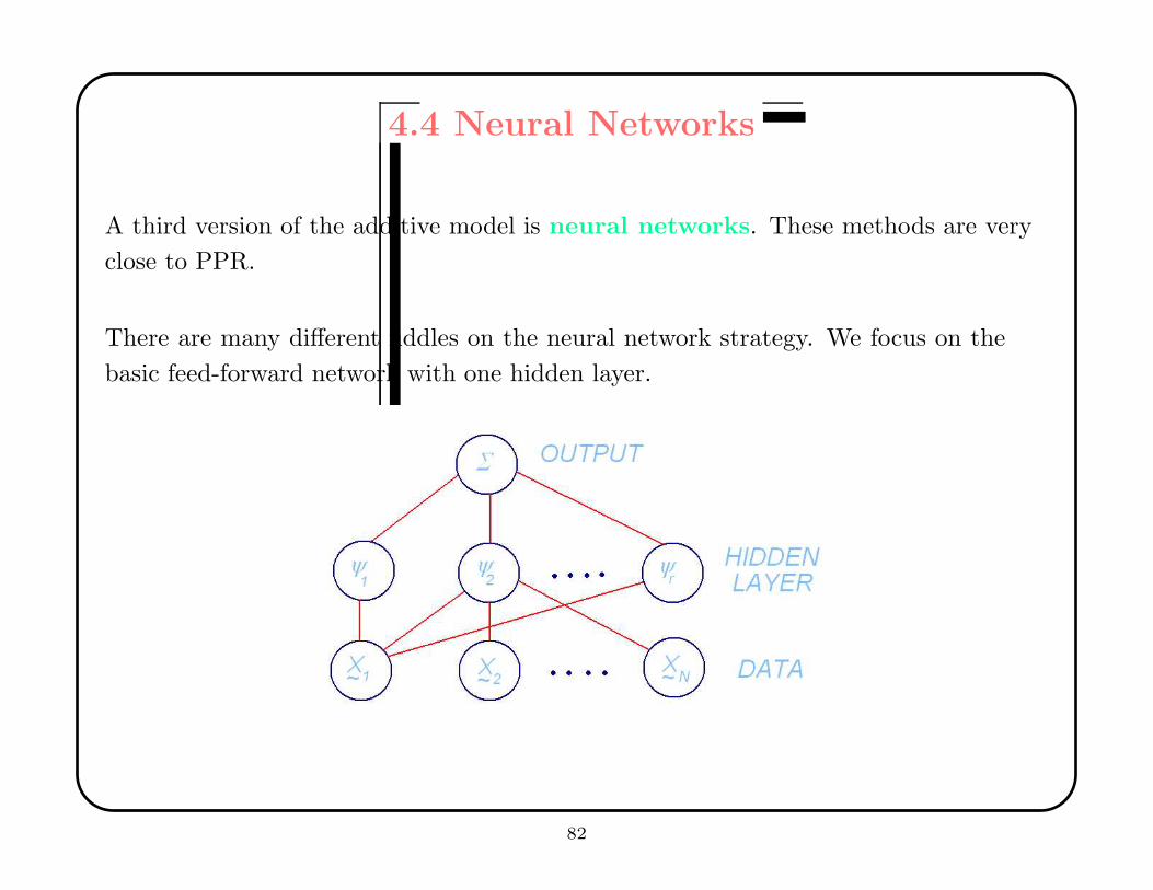
4.4 Neural Networks
A third version of the additive model is neural networks. These methods are very
close to PPR.
There are many different fiddles on the neural network strategy. We focus on the
basic feed-forward network with one hidden layer.
82
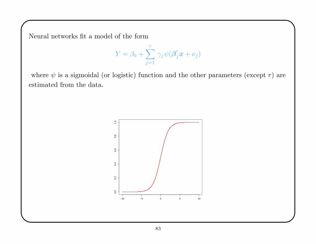
Neural networks fit a model of the form
Y = β0 +r∑
j=1
γjψ(β′jx + νj)
where ψ is a sigmoidal (or logistic) function and the other parameters (except r) are
estimated from the data.
−10 −5 0 5 10
0.0
0.2
0.4
0.6
0.8
1.0
83
The only difference between PPR and the neural net is that neural nets assumes that
the additive functions have a parametric (logistic) form:
ψ(x) =1
1 + exp(α0 + β′x).
The parametric assumption allows neural nets to be trained by backpropagation, an
iterative fitting technique. This is very similar to backfitting, but somewhat faster
because it does not require smoothing.
Barron (1993; IEEE Transactions on Information Theory, 39, 930-945) showed that
neural networks evade the Curse of Dimensionality in specific, rather technical, sense.
We sketch his result.
84
A standard way of assessing the performance of a nonparametric regression procedure
is in terms of Mean Integrated Square Error (MISE). Let g(x) denote the true
function and g(x) denote the estimated function. Then
MISE[g] = IEF
[∫
[g(x) − g(x)]2 dx
]
where the expectation is taken with respect to the randomness in the data {(Yi,Xi)}.
Before Barron’s work, it had been thought that the COD implied that for any
regression procedure, the MISE had to grow faster than linearly in p, the dimension
of the data. Barron showed that neural networks could attain an MISE of order
O(r−1) + O(rp/n) lnn where r is the number of hidden nodes.
Recall that an = O(h(n)) means there exists c such that for n sufficiently large,
an ≤ ch(n). Thus Barron’s error increases only linearly in p.
85

Barron’s theorem is technical. It applies to the class of functions g ∈ Γc on IRp whose
Fourier transforms g(ω) satisfy∫
|ω|g(ω) dω ≤ c
where the integral is in the complex domain and | · | denotes the complex modulus.
The class Γc is thick, meaning that it cannot be parameterized by a finite-dimensional
parameter. But it excludes important functions such as hyperflats.
The strategy in Barron’s proof is:
• Show that for all g ∈ Γc, there exists a neural net approximation g∗ such that
‖g − g∗‖2 ≤ c∗/n.
• Show that the MISE in estimating any of the g∗ functions is bounded.
• Combine these results to obtain a bound on the MISE of a neural net estimate g
for an arbitrary g ∈ Γc.
86
4.5 ACE and AVAS
Alternating Conditional Expectations (ACE) seeks transformations f1, . . . , fp
and g of the p explanatory variables and the response variable Y that maximize the
correlation between
g(Y ) and
p∑
j=1
fj(Xj).
This is equivalent to minimizing
IE[(g(Y ) −p∑
j=1
fj(Xj))2]/IE[g2(Y )]
where the expectations are taken with respect to {(Yi,Xi)}.
ACE modifies the additive modeling strategy by
• allowing arbitrary transformations of the response variable,
• using maximum correlation, squared error, for optimization.
87
ACE was developed by Breiman and Friedman (1985; Journal of the American
Statistical Association, 80, 580-619). It resembles canonical correlation.
The ACE algorithm works as follows:
1. Initialize. Set g(yi) = (yi − y)/sy; set fj(xj) as the regression of Y on Xj .
2. Backfit. Fit an additive model to g(y) to obtain new functions f1(x1), . . . , fp(xp).
3. Compute. Use smoothing to estimate
g(y) = IE[
p∑
j=1
fj(xj) |Yi = yi]
and standardize a new g(y) as
g(y) = g(y)/√
Var [g(y)].
(This standardization ensures that the trivial solution g ≡ 0 does not arise.)
4. Alternate. Do steps 2 and 3 until IE[(g(Y ) −∑p
j=1 fj(Xj))2] converges.
This finds the unique optimal solution, given by the eigenfunctions associated with
the largest eigenvalue of a certain operator.
88

intentional blank
89

intentional blank
90
From the standpoint of nonparametric regression, ACE has several undesirable
features.
• If g(Y ) = f(X) + ε, then ACE generally will not find g and f but rather h ◦ g and
h ◦ f .
• The solution is sensitive to the marginal distributions of the explanatory variables.
• ACE treats the explanatory and response variables in the same way, but
regression should be asymmetric.
• The eigenfunctions for the second-largest eigenvalue can provide better insight on
the problem.
There are a few other pathologies. See the discussion of the Breiman and Friedman
article for additional examples and details.
91
Additivity and Variance Stabilization (AVAS) is a modification of ACE that
removes most of the undesirable features. It was developed by Tibshirani (1988;
Journal of the American Statistical Association, 83, 394-405).
Heteroscedasticity is a common problem in regression and lies at the root of ACE’s
difficulties.
It is known that if a family of distributions for Z has mean µ and variance V (µ), then
the asymptotic variance stabilizing transformation for Z is
h(t) =
∫ t
0
V (s)−1/2 ds.
The AVAS algorithm is like the ACE algorithm except that in step 3 it applies the
estimated variance stabilizing transformation to g(Y ) before standardization.
92
4.6 Recursive Partitioning Regression
Partition methods are designed to handle surfaces with significant interaction
structure. The most famous of these methods is CART, for Classification and
Regression Trees (Breiman, Friedman, Olshen, and Stone; 1984, Wadsworth).
In regression, CART acts as a smart bin-smoother that performs automatic variable
selection. Formally, it fits the model
Y =r∑
j=1
βjI(x ∈ Rj) + ε
where the regions Rj and the coefficients βj are estimated from the data. Usually the
Rj are disjoint and the βj is the average of the Y values in Rj .
The CART model produces a decision tree that is helpful in interpreting the results,
and this is one of the keys to its enduring popularity.
93
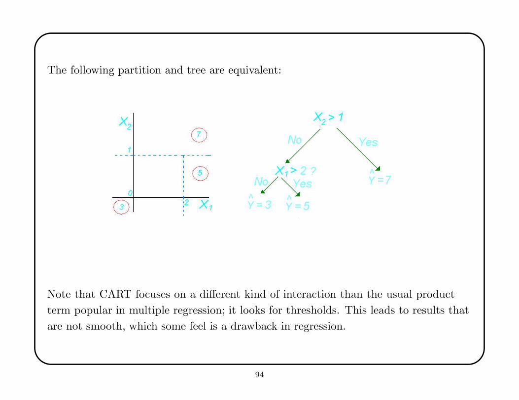
The following partition and tree are equivalent:
Note that CART focuses on a different kind of interaction than the usual product
term popular in multiple regression; it looks for thresholds. This leads to results that
are not smooth, which some feel is a drawback in regression.
94
The CART algorithm has three parts:
1. A way to select a split at each intermediate node.
2. A rule for declaring a node to be terminal.
3. A rule for estimating Y at a terminal node.
The third part is easy—just use the sample average of the cases at that terminal node.
The first part is also easy—split on the value x∗j which most reduces
SSerror =
n∑
i=1
(yi − fc(xi))2
Where fc is the predicted value from the current tree.
95
The second part is the hard one. One must grow an overly complicated tree, and then
use a pruning rule and cross-validation to find a tree with good predictive accuracy.
This entails a complexity penalty.
The main problems with CART are:
• discontinuous boundaries;
• it is difficult to approximate functions that are linear or additive in a small
number of variables;
• it is usually not competitive in low dimensions;
• one cannot tell when a complex CART model is close to a simple model.
The Boston housing data gives an example of the latter situation.
96
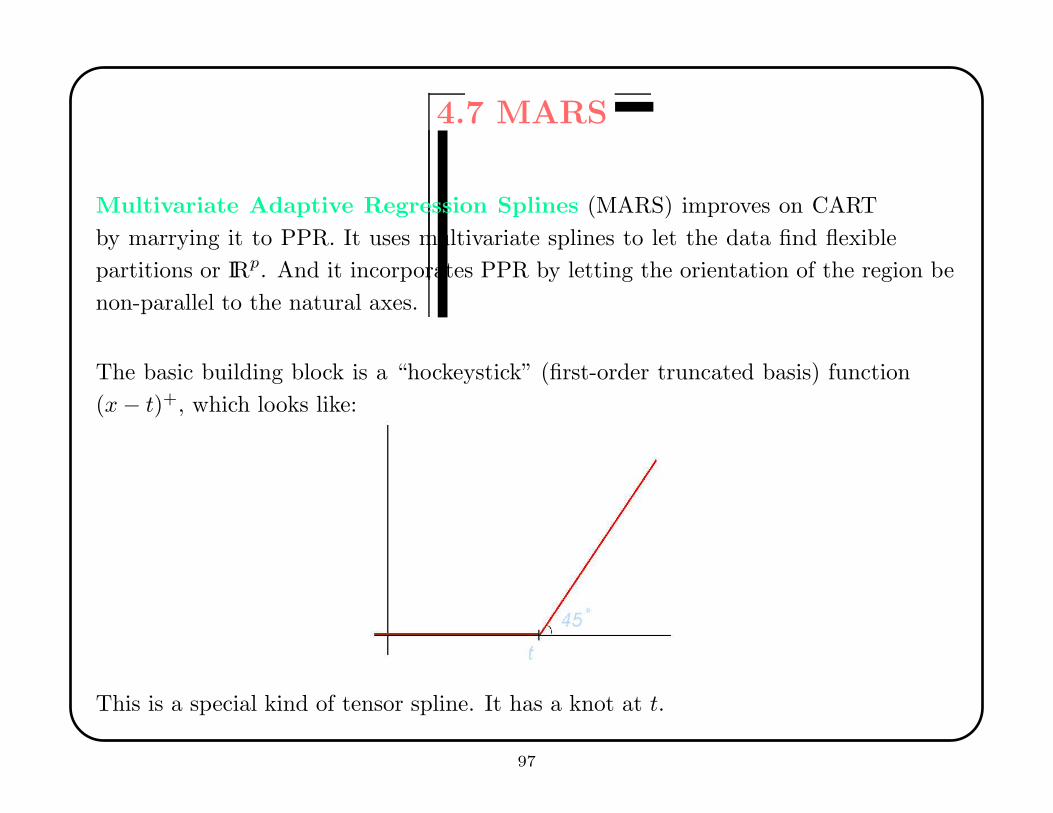
4.7 MARS
Multivariate Adaptive Regression Splines (MARS) improves on CART
by marrying it to PPR. It uses multivariate splines to let the data find flexible
partitions or IRp. And it incorporates PPR by letting the orientation of the region be
non-parallel to the natural axes.
The basic building block is a “hockeystick” (first-order truncated basis) function
(x− t)+, which looks like:
This is a special kind of tensor spline. It has a knot at t.
97
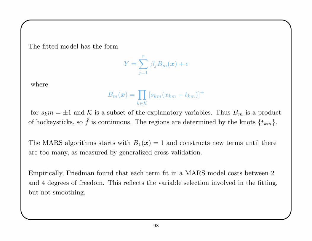
The fitted model has the form
Y =r∑
j=1
βjBm(x) + ε
where
Bm(x) =∏
k∈K[skm(xkm − tkm)]+
for skm = ±1 and K is a subset of the explanatory variables. Thus Bm is a product
of hockeysticks, so f is continuous. The regions are determined by the knots {tkm}.
The MARS algorithms starts with B1(x) = 1 and constructs new terms until there
are too many, as measured by generalized cross-validation.
Empirically, Friedman found that each term fit in a MARS model costs between 2
and 4 degrees of freedom. This reflects the variable selection involved in the fitting,
but not smoothing.
98

For each basis function Bm:
1. For all variables not in Bm,
A. try putting ± hockeysticks at every observation (candidate knot) in the
non-zero region of Bm;
B. select the best pair of hockeysticks according to an estimate of lack-of-fit.
2. Make two new basis functions from the product of Bm and the chosen pair of
hockeystick functions.
After building too many basis functions, prune back as in CART using
cross-validation.
Hockeysticks enter in pairs so that MARS is equivariant to sign changes.
Each Bm contains at most one term from each explanatory variable.
99

intentional blank
100
MARS is sort of interpretable, via an ANOVAesque decomposition:
f(x) = β0 +∑
j∈Jfj(xj) +
∑
(j,k)∈Kfjk(xj , xk) + . . .
where β0 is the coefficient of the B1 basis function, the first sum is over those basis
functions that involve a single explanatory variable, the second sum is over those
basis functions that involve exactly two explanatory variables, and so forth.
These terms can be thought of as the grand mean, the main effects, the two-way
interactions, etc. One can plot these functions to gain insight.
MARS uses a tensor product basis (hence no explanatory variable appears twice in
any Bm). Additive effects are captured by splitting B1 on several variables. Nonlinear
effects are captured by splitting B1 with the same variable more than once.
101

MARS and CART are available commercially from Salford Systems, Inc., and versions
of them are available in S+ and R.
To get an integrated suite of code that that performs ACE, AVAS, MARS, PPR,
neural nets (the CASCOR version), recursive partitioning, and Loess, one can
download the DRAT package from
www-2.cs.cmu.edu/∼bobski/software/software.html
There are many kinds of neural network code. Users should be careful in using
it—there are many possible twiddles and performance may vary. CASCOR is due to
Fahlman and Lebiere (1990; Advances in Neural Information Processing Systems 2,
524-532, Morgan Kaufmann), and has the convenience of adaptively choosing the
number of hidden nodes.
102
5. Comparing Methods
We have described eight methods so far: Loess, Additive Models (AM), PPR, Neural
Nets (NN), ACE, AVAS, Recursive Partitioning Regression (RPR), and MARS. In
addition, a practitioner might consider traditional stepwise linear regression (SLR)
and multiple linear regression (MLR).
One would like to make comparisons among these. In general, one would like to have
a practicum for making comparisons among complex statistical procedures that are
too difficult to analyze using theory.
This section describes a model simulation experiment, and it lays out the general
strategies for such comparisons.
103
Banks, Olszewski, and Maxion (2003; Communications in Statistics: Simulation and
Computation, 32, 541-571) describe a 10× 5× 34 designed experiment to compare the
methods.
The six factors in the experiment were:
1. The ten regression methods.
2. Five target functions.
3. The dimension: p = 2, 6, 12.
4. The sample size: n = 2pk for k = 4, 10, 25.
5. The proportion of spurious variables: this took the values all, half, and none.
6. The noise: this is the variance in ε, the additive Gaussian noise, and took the
values σ = .02, .1, .5.
104
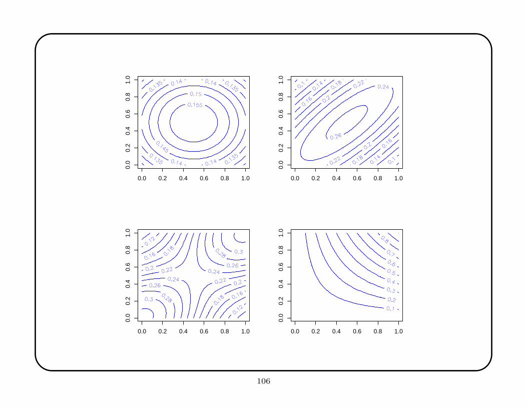
The target functions consist multivariate functions that approximate features likely to
be of scientific interest. The five functions are
• the constant function,
• the hyperflat,
• the standard normal recentered to (.5, . . . , .5)′,
• a normal centered (.5, . . . , .5)′ with covariance matrix .8I
• a mixture of two standard normals, one centered at (0, . . . , 0)′ and the other at
(1, . . . , 1)′
• the product function x1x2 · · ·xp.
The constant function is especially important because in that case the explanatory
values are irrelevant, but some methods tend to discover spurious signal in the noise.
105
0.0 0.2 0.4 0.6 0.8 1.0
0.0
0.2
0.4
0.6
0.8
1.0
0.0 0.2 0.4 0.6 0.8 1.0
0.0
0.2
0.4
0.6
0.8
1.0
0.0 0.2 0.4 0.6 0.8 1.0
0.0
0.2
0.4
0.6
0.8
1.0
0.0 0.2 0.4 0.6 0.8 1.0
0.0
0.2
0.4
0.6
0.8
1.0
106
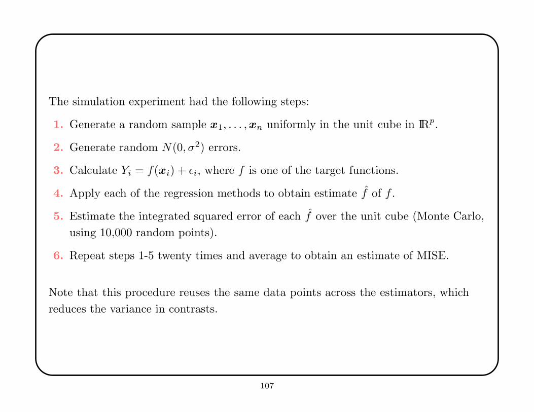
The simulation experiment had the following steps:
1. Generate a random sample x1, . . . ,xn uniformly in the unit cube in IRp.
2. Generate random N(0, σ2) errors.
3. Calculate Yi = f(xi) + εi, where f is one of the target functions.
4. Apply each of the regression methods to obtain estimate f of f .
5. Estimate the integrated squared error of each f over the unit cube (Monte Carlo,
using 10,000 random points).
6. Repeat steps 1-5 twenty times and average to obtain an estimate of MISE.
Note that this procedure reuses the same data points across the estimators, which
reduces the variance in contrasts.
107
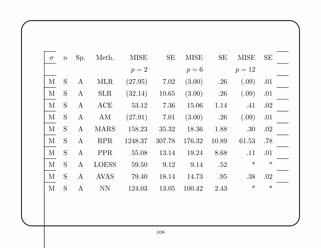
σ n Sp. Meth. MISE SE MISE SE MISE SE
p = 2 p = 6 p = 12
M S A MLR (27.95) 7.02 (3.00) .26 (.09) .01
M S A SLR (32.14) 10.65 (3.00) .26 (.09) .01
M S A ACE 53.12 7.36 15.06 1.14 .41 .02
M S A AM (27.91) 7.01 (3.00) .26 (.09) .01
M S A MARS 158.23 35.32 18.36 1.88 .30 .02
M S A RPR 1248.37 307.78 176.32 10.89 61.53 .78
M S A PPR 55.08 13.14 19.24 8.68 .11 .01
M S A LOESS 59.50 9.12 9.14 .52 * *
M S A AVAS 79.40 18.14 14.73 .95 .38 .02
M S A NN 124.03 13.05 100.42 2.43 * *
108
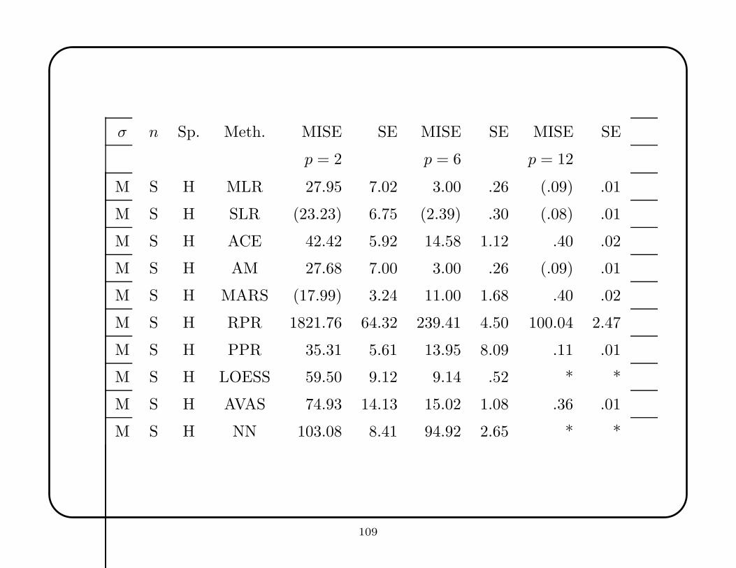
σ n Sp. Meth. MISE SE MISE SE MISE SE
p = 2 p = 6 p = 12
M S H MLR 27.95 7.02 3.00 .26 (.09) .01
M S H SLR (23.23) 6.75 (2.39) .30 (.08) .01
M S H ACE 42.42 5.92 14.58 1.12 .40 .02
M S H AM 27.68 7.00 3.00 .26 (.09) .01
M S H MARS (17.99) 3.24 11.00 1.68 .40 .02
M S H RPR 1821.76 64.32 239.41 4.50 100.04 2.47
M S H PPR 35.31 5.61 13.95 8.09 .11 .01
M S H LOESS 59.50 9.12 9.14 .52 * *
M S H AVAS 74.93 14.13 15.02 1.08 .36 .01
M S H NN 103.08 8.41 94.92 2.65 * *
109
MLR, SLR, and AM perform similarly over all situations considered, and represent
broadly safe choices. They are never disastrous, though rarely the best (except for
MLR when the target function is linear and all variables are used). For the constant
function, SLR shows less overfit than MLR, which is better than AM; however, it is
easy to find functions for which AM would outperform both MLR and SLR. SLR
is usually slightly better with spurious variables, but its strategy becomes notably
less effective as the number of spurious variables increases, especially for non-linear
functions. All three methods have greatest relative difficulty with the product
function, which has substantial curvature.
On theoretical grounds ACE and AVAS should be similar, but this is not always
borne out. ACE is decisively better for the product function, and AVAS for the
constant function. ACE and AVAS are the best methods for the product function
(as expected—the log transformation produces a linear relationship), but among the
worst for the constant function and the mixture of Gaussians; in other cases, their
performance is not remarkable. Both methods are fairly robust to spurious variables.
110
Contrary to expectation, MARS does not show well in higher dimensions, especially
when all variables are used, and especially for the linear function. However, for lower
dimensions, MARS shows adequate performance across the different functions. MARS
is well-calibrated for the constant function when p = 2, but finds spurious structure
for larger values, which may account for some of its failures.
RPR was consistently bad in low dimensions, but sometimes stunningly successful in
high dimensions, especially when all variables were used. Surprisingly, its variable
selection capability was not very successful (MARS’s implementation clearly
outperforms it). Perhaps the CART program, with its flexible pruning, would surpass
RPR, but previous experience with CART makes us dubious. Unsurprisingly, RPR’s
design made it uncompetitive on the linear function.
111
PPR and NN are theoretically similar methods, but PPR was clearly superior in all
cases except the correlated Gaussian. This may reflect peculiarities of the Cascor
implementation of neural nets. PPR was often among the best when the target
function was the Gaussian, correlated Gaussian, or mixture of Gaussians, but
among the worst with the product and constant functions. PPR’s variable selection
was generally good. In contrast, NN was generally poor, except for the correlated
Gaussian when p = 2, 6 and all variables are used and when p = 6 and half the
variables are used. The correlated Gaussian lends itself to approximation by a small
number of sigmoidal functions whose orientations are determined by the data.
LOESS does well in low dimensions with the Gaussian, correlated Gaussian, and
mixture of Gaussians. It is not as successful with the other target functions, especially
the constant function. Often, it is not bad in higher dimensions, though its relative
performance tends to deteriorate.
112
For the constant function, MARS is good when p = 2, SLR is good when p = 6, and
RPR is good when p = 12. For the linear function, MLR and SLR are consistently
strong. For the Gaussian function, with all variables used, LOESS and MARS are
good when p = 2, SLR is good when p = 6, and RPR is good when p = 12; when half
of the variables are used, MARS and PPR perform well. For the correlated Gaussian,
with all variables used, LOESS works well for p = 2, LOESS and NN for p = 6, and
ACE or AVAS for p = 12; with half the variables used, MARS is reliably good. For
the mixture of Gaussians, with all variables used, LOESS works well for p ≤ 6, and
RPR for p = 12; with half of the variables, MARS is consistently good. There is
considerable variability for the product function, but ACE is broadly superior.
Two kinds of variable selection strategies were used by the methods: global variable
selection, as practiced by SLR, ACE, AVAS, and PPR, and local variable reduction,
as practiced by MARS and RPR. Generally, the latter does best in high dimensions,
but performance depends on the target function.
113
LOESS, NN, and sometimes AVAS proved infeasible in high dimensions. The number
of local minimizations in LOESS grew exponentially with p. Cascor’s demands
were high because of the cross-validated selection of the hidden nodes; alternative
NN methods fix these a priori, making fewer computational demands, but this is
equivalent to imposing strong, though complex, modeling assumptions. Typically,
fitting a single high-dimensional dataset with either LOESS or NN took more than
two hours. AVAS was faster, but the combination of high dimension and large sample
size also required substantial time.
114

intentional blank
115

6. Local Dimension
Nearly all methods for multivariate nonparametric regression do local model fitting
(otherwise, they must make strong model assumptions, such as multiple linear
regression). Local fitting is most likely to succeed if the response function f(x) has
locally-low dimension.
A function f : IRp → IR has locally-low dimension if there exists a set of regions
R1, R2, . . . and a set of functions g1, g2, . . . such that⋃
Ri ≈ IRp and for x ∈ Ri,
f(x).= gi(x) where gi depends upon only q components of x for q � p.
This uses a vague sense of approximation, but it can be made precise.
116
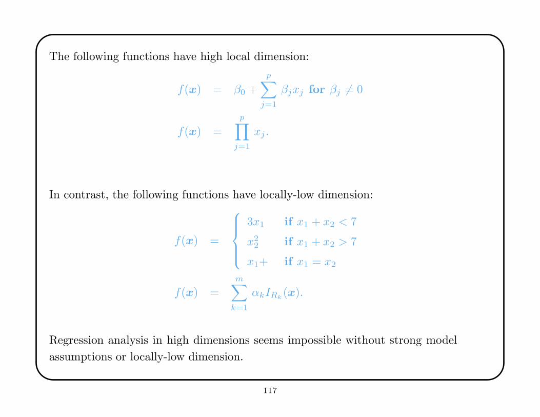
The following functions have high local dimension:
f(x) = β0 +
p∑
j=1
βjxj for βj 6= 0
f(x) =
p∏
j=1
xj .
In contrast, the following functions have locally-low dimension:
f(x) =
3x1 if x1 + x2 < 7
x22 if x1 + x2 > 7
x1+ if x1 = x2
f(x) =
m∑
k=1
αkIRk(x).
Regression analysis in high dimensions seems impossible without strong model
assumptions or locally-low dimension.
117
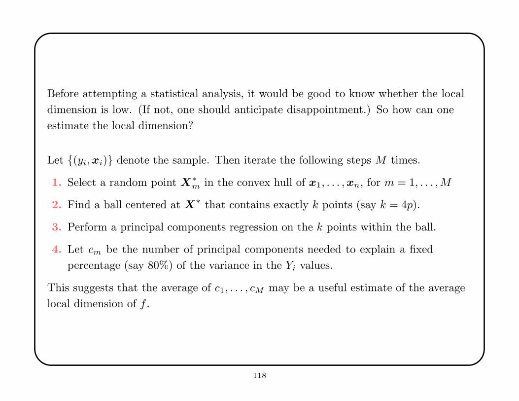
Before attempting a statistical analysis, it would be good to know whether the local
dimension is low. (If not, one should anticipate disappointment.) So how can one
estimate the local dimension?
Let {(yi,xi)} denote the sample. Then iterate the following steps M times.
1. Select a random point X∗m in the convex hull of x1, . . . ,xn, for m = 1, . . . ,M
2. Find a ball centered at X∗ that contains exactly k points (say k = 4p).
3. Perform a principal components regression on the k points within the ball.
4. Let cm be the number of principal components needed to explain a fixed
percentage (say 80%) of the variance in the Yi values.
This suggests that the average of c1, . . . , cM may be a useful estimate of the average
local dimension of f .
118
This heuristic approach assumes a locally linear functional relationship for points
within the ball. The Taylor series motivates this, but the method will break down for
some pathological functions or if the data are too sparse.
To test the approach, Banks and Olszewski (2003; Statistical Data Mining and
Knowledge Discovery, 529-548, Chapman & Hall) performed a simulation experiment
in which random samples were generated from q-cube submanifolds in IRp, and the
approach described above was used to estimate q.
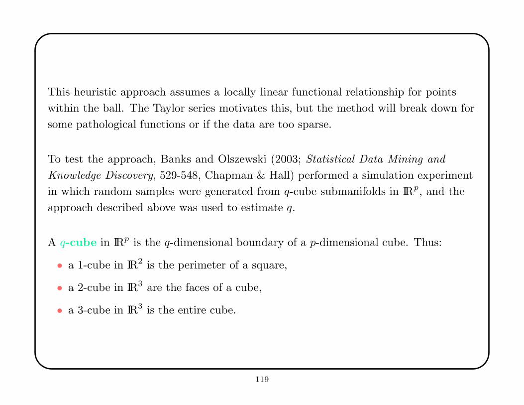
A q-cube in IRp is the q-dimensional boundary of a p-dimensional cube. Thus:
• a 1-cube in IR2 is the perimeter of a square,
• a 2-cube in IR3 are the faces of a cube,
• a 3-cube in IR3 is the entire cube.
119

The following figure shows a 1-cube in IR3, tilted 10 degrees from the natural axes in
each coordinate.
120
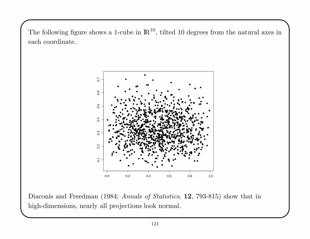
The following figure shows a 1-cube in IR10, tilted 10 degrees from the natural axes in
each coordinate.
0.0 0.2 0.4 0.6 0.8 1.0
0.1
0.2
0.3
0.4
0.5
0.6
0.7
Diaconis and Freedman (1984; Annals of Statistics, 12, 793-815) show that in
high-dimensions, nearly all projections look normal.
121
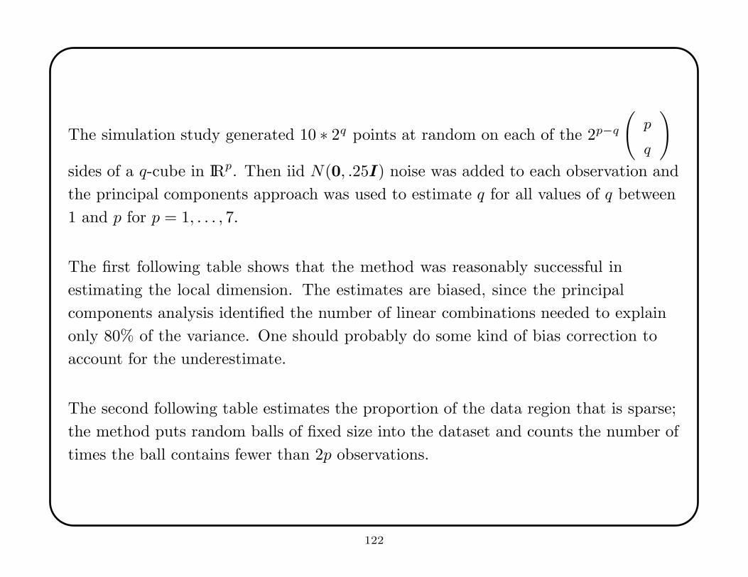
The simulation study generated 10 ∗ 2q points at random on each of the 2p−q
(
p
q
)
sides of a q-cube in IRp. Then iid N(0, .25I) noise was added to each observation and
the principal components approach was used to estimate q for all values of q between
1 and p for p = 1, . . . , 7.
The first following table shows that the method was reasonably successful in
estimating the local dimension. The estimates are biased, since the principal
components analysis identified the number of linear combinations needed to explain
only 80% of the variance. One should probably do some kind of bias correction to
account for the underestimate.
The second following table estimates the proportion of the data region that is sparse;
the method puts random balls of fixed size into the dataset and counts the number of
times the ball contains fewer than 2p observations.
122
q
7 5.03
6 4.25 4.23
5 3.49 3.55 3.69
4 2.75 2.90 3.05 3.18
3 2.04 2.24 2.37 2.50 2.58
2 1.43 1.58 1.71 1.80 1.83 1.87
1 .80 .88 .92 .96 .95 .95 .98
p=1 2 3 4 5 6 7
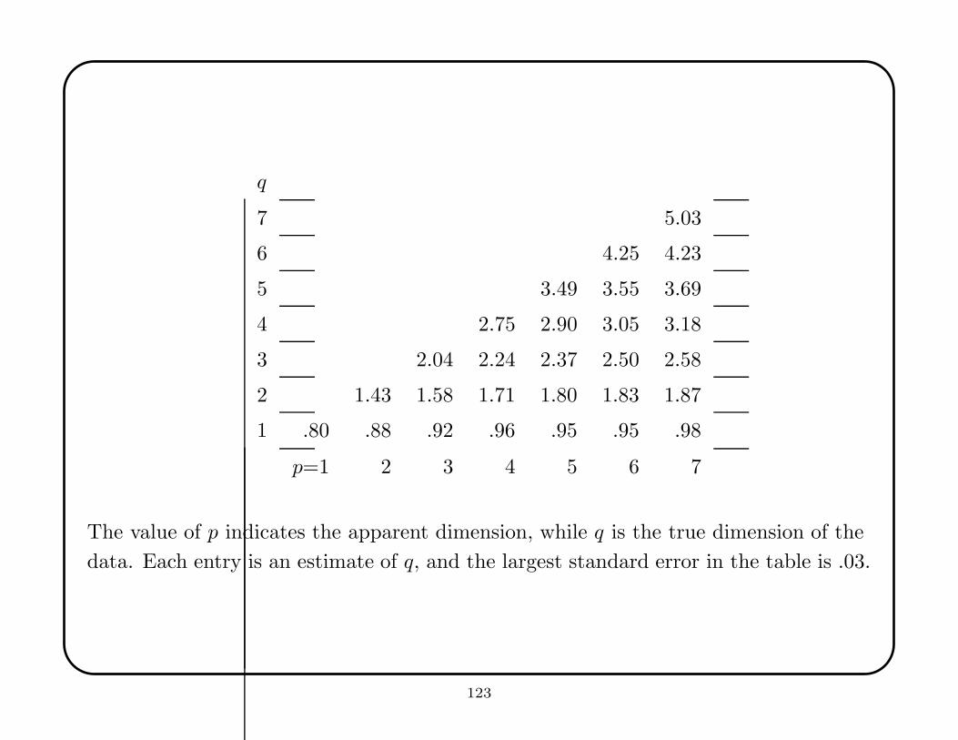
The value of p indicates the apparent dimension, while q is the true dimension of the
data. Each entry is an estimate of q, and the largest standard error in the table is .03.
123
q
7 41.0
6 39.1 52.2
5 34.4 45.3 53.2
4 32.3 36.2 46.1 55.9
3 29.1 27.0 34.7 48.6 57.9
2 28.4 26.5 32.0 41.6 46.6 55.2
1 28.5 40.1 45.8 51.0 51.3 51.0 52.5
p=1 2 3 4 5 6 7
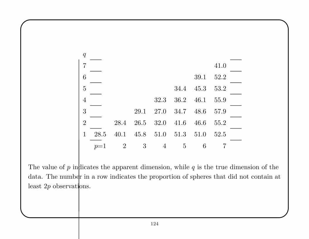
The value of p indicates the apparent dimension, while q is the true dimension of the
data. The number in a row indicates the proportion of spheres that did not contain at
least 2p observations.
124
7. Classification
Classification problems attempt to find rules that assign cases to categories, e.g.:
• correct versus incorrect tax returns
• medical diagnoses
• good versus bad credit risks
• terrorists versus non-terrorists.
One uses a training sample of cases for which the categories are known. Each case has
a vector of covariates that are used to build the classification rule.
For a new observation, one looks at its covariate and classifies it according to the
classification rule.
125
There are three main strategies for building classification rules:
• Geometric, which includes discriminant analysis, flexible discriminant analysis,
and recursive partitioning.
• Algorithmic, which includes neural nets, nearest neighbor rules, support vector
machines, and random forests.
• Probabilistic, which includes Bayes rules and hidden Markov models.
The probabilistic methods make strong assumptions about having random samples of
data.
Most classification problems are very similar to regression problems. For problems
with two categories, it is sometimes just a matter of fitting a model that predicts 1 or
−1 according to the case label.
126
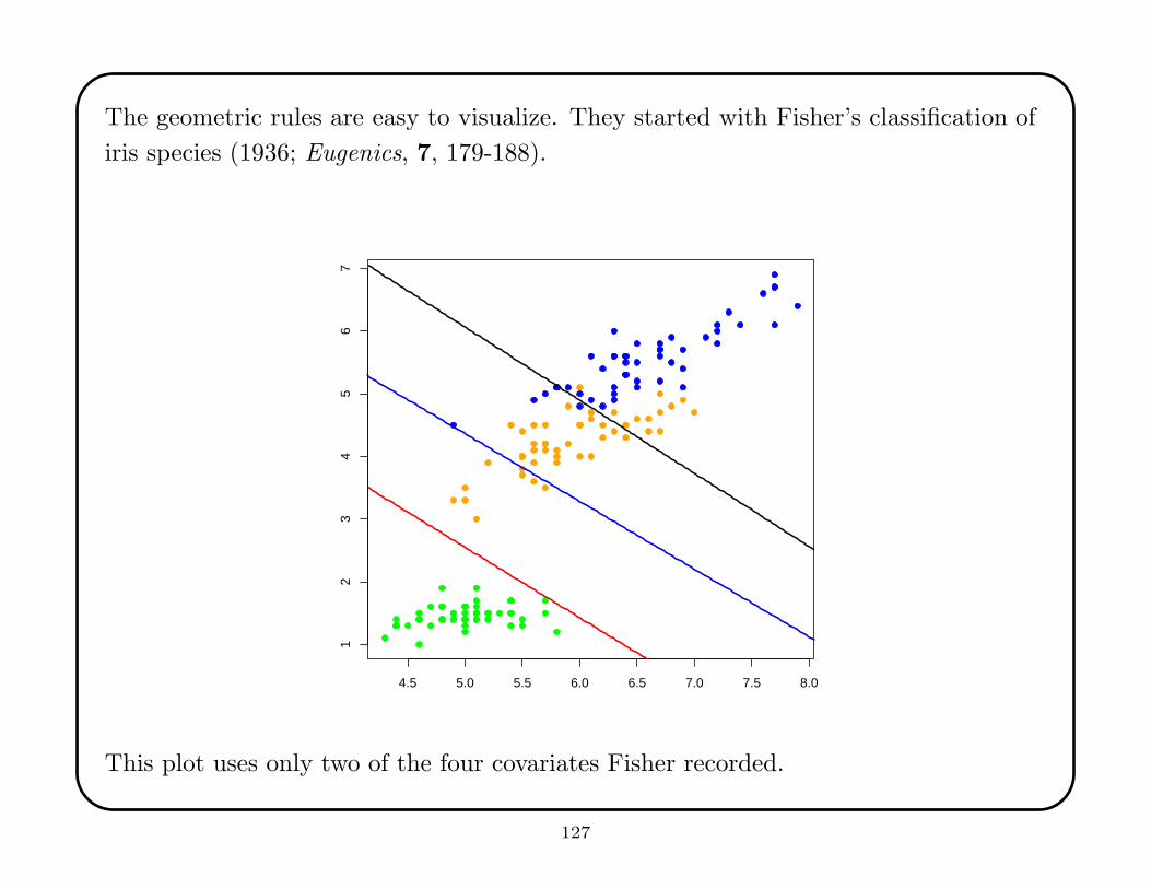
The geometric rules are easy to visualize. They started with Fisher’s classification of
iris species (1936; Eugenics, 7, 179-188).
4.5 5.0 5.5 6.0 6.5 7.0 7.5 8.0
12
34
56
7
This plot uses only two of the four covariates Fisher recorded.
127
For two classes, Fisher’s linear discriminant analysis assumes that the two populations
have multivariate normal distribution with common unknown covariance matrix and
different unknown mean vectors. It assigns a new observation to the population whose
mean has the smallest Mahalanobis distance to the observation:
dM (xi, xj) = [(xi − xj)′S−1(xi − xj)]
1/2
To analyze the effect of noise in linear discriminant analysis, suppose one has a fixed
sample size n and assume the covariance matrices are known to be σ2I . Write the
estimates of the means as:
µ1 = µ1 +σ√n
v1
µ2 = µ2 +σ√n
v2.
Also, write the new observation to classify as:
x = µ1 + v.
128
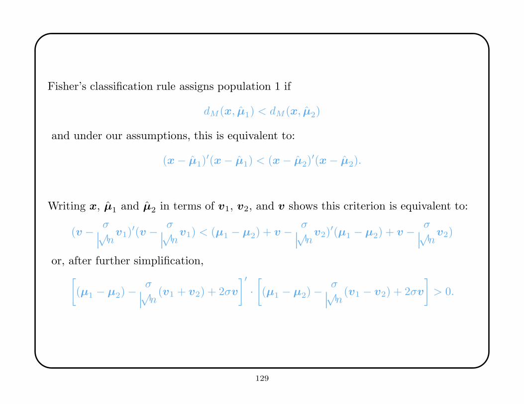
Fisher’s classification rule assigns population 1 if
dM (x, µ1) < dM (x, µ2)
and under our assumptions, this is equivalent to:
(x − µ1)′(x − µ1) < (x − µ2)
′(x − µ2).
Writing x, µ1 and µ2 in terms of v1, v2, and v shows this criterion is equivalent to:
(v − σ√n
v1)′(v − σ√
nv1) < (µ1 − µ2) + v − σ√
nv2)
′(µ1 − µ2) + v − σ√n
v2)
or, after further simplification,
[
(µ1 − µ2) −σ√n
(v1 + v2) + 2σv
]′·[
(µ1 − µ2) −σ√n
(v1 − v2) + 2σv
]
> 0.
129
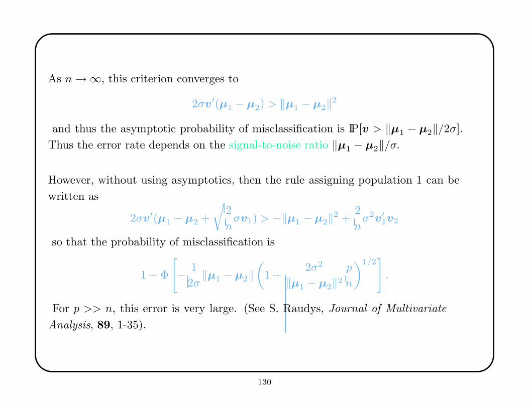
As n→ ∞, this criterion converges to
2σv′(µ1 − µ2) > ‖µ1 − µ2‖2
and thus the asymptotic probability of misclassification is IP[v > ‖µ1 − µ2‖/2σ].
Thus the error rate depends on the signal-to-noise ratio ‖µ1 − µ2‖/σ.
However, without using asymptotics, then the rule assigning population 1 can be
written as
2σv′(µ1 − µ2 +
√
2
nσv1) > −‖µ1 − µ2‖2 +
2
nσ2v′
1v2
so that the probability of misclassification is
1 − Φ
[
− 1
2σ‖µ1 − µ2‖
(
1 +2σ2
‖µ1 − µ2‖2
p
n
)1/2]
.
For p >> n, this error is very large. (See S. Raudys, Journal of Multivariate
Analysis, 89, 1-35).
130

intentional blank
131
A very reasonable approach to classification is kth nearest-neighbor classification. In
order to make a prediction about a new observation, one looks at the labels of its k
nearest neighbors and uses a majority vote to make the prediction.
As the number of neighbors used in making the prediction increases, the decision
boundaries become smoother—the bias increases, but the variance decreases. The
“degrees-of-freedom” for nearest-neighbor rules is n/k.
The following images show how nearest-neighbor classification rules peform on data
simulated from a 20-component mixture of normals, half of which were red, half of
which were green. The effect of the bias-variance tradeoff is quite clear.
132

intentional blank
133

intentional blank
134

intentional blank
135

intentional blank
136
intentional blank
137
intentional blank
138

intentional blank
139
7.1 Support Vector Machines
Support Vector Machines (SVMs) were invented by Vapnik (1996; The Nature of
Statistical Learning, Springer). They use optimization methods to find surfaces that
best separate categories.
SVMs have been developed in many different directions, and have become quite
elaborate. This survey focuses upon classifying two groups, and develop the ideas in
three steps:
• Linear machines trained on separable classes;
• Linear machines trained on overlapping classes;
• Nonlinear machines.
140
7.1.1 Linear Machines, Separable Data
Suppose the n observations are {(xi, yi)} where xi ∈ IRp and yi ∈ {−1, 1}. And
suppose one seeks a simple linear classification rule of the form
g(x) = sign[βT x + β0]
where β is determined from the data. (WLOG, assume ‖β‖ = 1.)
If the two classes are separable then there are many possible β that work. A natural
strategy is to pick the β that creates the biggest margin between the two classes.
The margin is twice perpendicular distance from the closest value with label +1 to the
separating hyperflat (or the sum of the two smallest distances, one from each class).
141

intentional blank
142
Denote the margin by d. Then the optimization problem is to
maxβ,β0,‖β‖=1
d
subject to yi(βT xi + β0) ≥ d, i = 1, . . . n.
One can rewrite this as a convex optimization problem with with a quadratic criterion
and linear constraints:
min ‖β‖subject to yi(β
T xi + β0) ≥ 1, i = 1, . . . n
where the requirement that β have unit norm is dropped. It turns out that
d = ‖β‖−1.
Note that
• this solution is not equivalent to the one obtained from linear discriminant
analysis;
• the solution depends only upon the two closest points in the two classes.
143
To solve the rewritten problem we can use a Lagrangian:
L =1
2‖β‖2 −
n∑
i=1
λiyi(x′iβ + β0) +
n∑
i=1
λi
The goal is to minimize L with respect to β and β0, while simultaneously requiring
λi ≥ 0 and that the derivatives of L with respect to the λi vanish.
The Lagrangian formulation has two advantages:
• the original constraints are replaced by constraints on the Lagrange multipliers,
which are easier to handle;
• the training data only appear once, as dot products in a sum, which allows
generalization to nonlinear machines.
144
The dual problem of the Lagrangian minimization is to maximize L subject to:
0 =∂L
∂βifor all i
0 =∂L
∂β0
0 ≤ λi for all i.
This is called the Wolfe dual (see Fletcher, 1987, Practical Methods of Optimization,
Wiley).
The zero-gradient requirement generates equality constraints, leading to
LD =n∑
i=1
λi −1
2
∑
i,j
λiλjyiyjx′ixj
which is maximized under the constraint that∑n
i=1 λiyi = 0 and λi ≥ 0 for all i.
145
Training the SVM amounts to solving this optimization problem. We used a
primal-dual solution, but anything that satisfies the Karush-Kuhn-Tucker conditions
will be necessary and sufficient.
Note that for each observation, there is a Lagrange multiplier λi. Those observations
with λi > 0 are the support vectors, and determine the margin. For all the other
observations the λi are zero. If the problem were reworked using only the support
vectors data, the same solution would be found.
Also note that the β0 is determined implicitly. Solve
λi[yi(β′xi + β0) − 1] = 0
using any support vector observation.
146
7.1.2 Linear Machines, Nonseparable Data
In practice, it usually happens that the two classes are not separable. In that case one
wants to find the hyperflat that minimizes the sum of the perpendicular distances for
the data that violate the rule. This leads to a slightly more advanced optimization
problem that includes slack variables. This can be solved using Lagrange multipliers.
Cortes and Vapnik (1995; Machine Learning, 20, 273-297) developed support vector
machines to extend the optimization strategy we have described.
One can also view this as a problem in physics, in which each of the support vectors
exerts a force on a rigid sheet. The equilibrium solution determines the separator.
147

7.1.3 Nonlinear Machines
The mathematics in the SVM literature can be serious, but the key idea is to find
linear combinations of basis functions of x that describe good separating surfaces.
As previously noted, in real problems one wants more flexible separating surfaces
than hyperflats. Boser, Guyon, and Vapnik (1992; Fifth Annual Workshop on
Computational Learning Theory, ACM) showed how to do this in the SVM context,
using an old idea of Aizerman et al. (1964; Automation and Remote Control, 25,
821-837).
The main innovation is to express the surfaces in terms of a vastly expanded set of
basis functions. SVMs map the problem to a higher dimensional space, and then solve
the linear separation problem using nonlinear basis elements.
148
Consider the problem of building a classification rule for just two types of objects,
where each object has measurements in IRp. One can find separating hyperplanes or
quadratic surfaces, as in linear or quadratic discriminant analysis, or one can fit more
complex separating surfaces.
In principle, one would like to be able to fit very curvy surfaces, when the data
warrant, that can separate complex structure in the two classes. Such surfaces can be
formed by linear combinations of basis functions.
Recall that some of the standard basis sets are the Fourier basis, the Legendre
polynomials, and so forth.
A basis set is set of functions {fi} such that any function g in the space can be
written as
g(x) =∞∑
i=1
βifi(x)
and no element of {fi} can be written as a linear combination of the other elements.
149
The SVM strategy is to greatly expand the dimension of the input space beyond p,
and then find hyperflats in that expanded space that classify the training sample.
Then one maps back down to the lower-dimensional space, and it generally happens
that the linear separating rules in the high-dimensional space become non-linear rules
in the p dimensional space.
Consider expanding the set of inputs to include additional functions of the inputs, say
h(xi) = (h1(xi, . . . , hq(xi))T . If these are just a single component of the xi data then
q = p and this reduces to the simple case described in 7.1.1.
One can show that the separating surface has the form
g(x) =n∑
i=1
βi < h(x),h(xi) > +β0
where < ·, · > denotes an inner product.
150
Formally, suppose we use a mapping H to take the data from IRp to a (possibly
infinite-dimensional) Euclidean space H.
Recall that the optimization problem can be written so that it only depends upon dot
products of the data, x′ixj . Thus after the mapping, the solution in H depends only
upon functions of the form h(xi)′h(xj).
Therefore it is sufficient to find a function
K(xi,xj) = h(xi)′h(xj).
The nice thing is that we do not need to know the mapping H .
151
Determining the functions in h(x) turns out to be equivalent to selecting a basis for a
particular subspace. This depends upon a kernel function.
A kernel function is a positive semidefinite function
K(x,x∗) = < h(x),h(x∗) >
=
q∑
j=1
hj(x)hj(x∗).
This is related to reproducing kernel Hilbert spaces.
Three common choices for kernel functions in SVM applications are:
• K(x,x∗) = exp(−‖x − x∗‖2/c), known as the radial basis;
• K(x,x∗) = tanh(α1 < x,x∗ > +α2), or the neural network basis; and
• K(x,x∗) = (1+ < x,x∗ >)r, the rth degree polynomials.
152
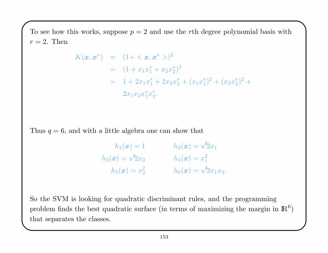
To see how this works, suppose p = 2 and use the rth degree polynomial basis with
r = 2. Then
K(x,x∗) = (1+ < x,x∗ >)2
= (1 + x1x∗1 + x2x
∗2)
2
= 1 + 2x1x∗1 + 2x2x
∗2 + (x1x
∗1)
2 + (x2x∗2)
2 +
2x1x2x∗1x
∗2.
Thus q = 6, and with a little algebra one can show that
h1(x) = 1 h2(x) =√
2x1
h3(x) =√
2x2 h4(x) = x21
h5(x) = x22 h6(x) =
√2x1x2.
So the SVM is looking for quadratic discriminant rules, and the programming
problem finds the best quadratic surface (in terms of maximizing the margin in IR6)
that separates the classes.
153
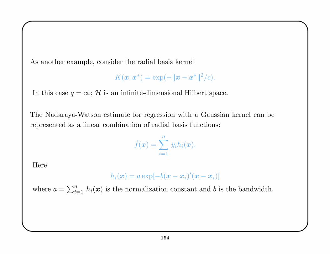
As another example, consider the radial basis kernel
K(x,x∗) = exp(−‖x − x∗‖2/c).
In this case q = ∞; H is an infinite-dimensional Hilbert space.
The Nadaraya-Watson estimate for regression with a Gaussian kernel can be
represented as a linear combination of radial basis functions:
f(x) =n∑
i=1
yihi(x).
Here
hi(x) = a exp[−b(x − xi)′(x − xi)]
where a =∑n
i=1 hi(x) is the normalization constant and b is the bandwidth.
154
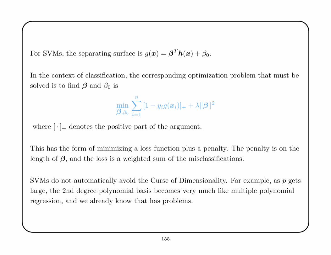
For SVMs, the separating surface is g(x) = βT h(x) + β0.
In the context of classification, the corresponding optimization problem that must be
solved is to find β and β0 is
minβ,β0
n∑
i=1
[1 − yig(xi)]+ + λ‖β‖2
where [ · ]+ denotes the positive part of the argument.
This has the form of minimizing a loss function plus a penalty. The penalty is on the
length of β, and the loss is a weighted sum of the misclassifications.
SVMs do not automatically avoid the Curse of Dimensionality. For example, as p gets
large, the 2nd degree polynomial basis becomes very much like multiple polynomial
regression, and we already know that has problems.
155
7.2 Trees and Random Forests
Recursive partitioning is used for classification as well as regression. CART (Breiman,
Friedman, Olshen, and Stone, 1984, Classification and Regression Trees, Wadsworth)
is the most famous of these methods.
A classification tree starts with a training sample of n cases with known categories.
Case i has a vector of covariates xi, and those are used to build a tree-structured
classification rule.
Recursive partitioning is one of the most popular data mining tools, in large part
because the tree-structured decision rule is easy to represent and often easy to
interpret.
156
Formally, recursive partitioning splits the training sample into increasingly
homogeneous groups, thus inducing a partition on the space of explanatory variables.
At each step, the algorithm considers three possible kinds of splits using the vector of
explanatory values x:
1. Is xi ≤ t? (univariate split)
2. Is∑p
i=1 wixi ≤ t? (linear combination split)
3. Does xiεS? (categorical split, used if xi is a categorical variable).
The algorithm searches over all possible values of t, all coefficients {wi}, and all
possible subsets S of the category values to find the split that best separates the cases
in the training sample into two groups with maximum increase in overall homogeneity.
157

intentional blank
158
Different partitioning algorithms use different methods for assessing improvement in
homogeneity. Classical methods seek to minimize Gini’s index of diversity, or use a
“twoing rule.” Hybrid methods can switch criteria as they move down the decision
tree.
Similarly, some methods seek to find the greatest improvement on both sides of the
split, whereas other methods choose the split that achieves maximum homogeneity on
one side or the other.
Some methods grow elaborate trees, and then prune back to improve predictive
accuracy outside the training sample (this is a partial response to the kinds of overfit
concerns that arise from the Curse of Dimensionality).
The result is a decision tree. The following figure shows a famous application that
assesses whether or not an emergency room patient is at risk for a second heart attack.
159
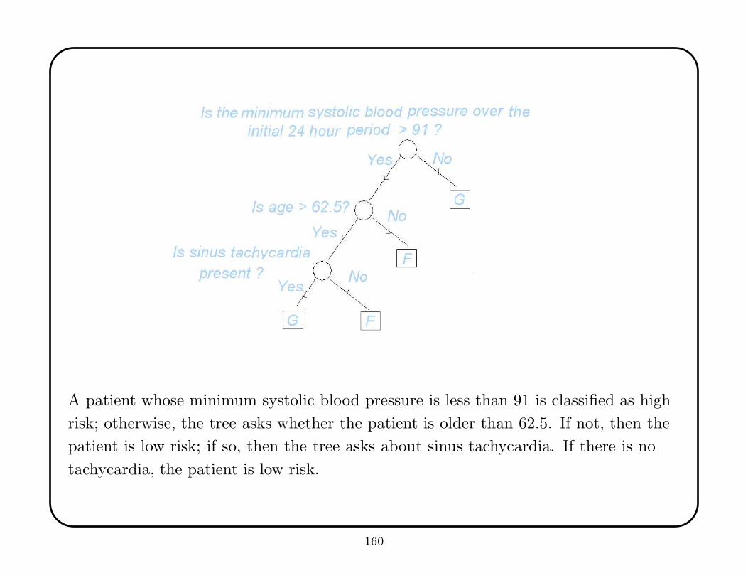
A patient whose minimum systolic blood pressure is less than 91 is classified as high
risk; otherwise, the tree asks whether the patient is older than 62.5. If not, then the
patient is low risk; if so, then the tree asks about sinus tachycardia. If there is no
tachycardia, the patient is low risk.
160

intentional blank
161

intentional blank
162

intentional blank
163
A random forest is a collection of identically distributed trees. Each tree is
constructed by some tree classification algorithm such as CART.
The random forest is formed by taking bootstrap samples from the training set. For
each bootstrap sample, a classification tree is formed, and there is no pruning—the
tree grows until all terminal nodes are pure.
After the tree is grown, one drops a new case down each of the trees. The classification
that receives the majority vote is the one that is assigned.
Random forests were invented by Breiman (2001; Machine Learning, 45, 5-32).
164
The key features of random forests include:
• It is a good classifier—fully competitive with SVMs.
• It generates an internal unbiased estimate of the generalization error.
• It handles missing data very well, and can maintain high levels of accuracy when
up to 80% of the data are missing at random.
• It provides estimates of the relative importance of each of the covariates in the
classification rule.
• It computes proximities between pairs of cases that can be used in clustering,
identifying outliers, and multidimensional scaling.
• It can be applied with unlabelled data, leading to unsupervised clustering.
• It can rebalance the weights when the category proportions in the training data
do not reflect the category proportions in the true population.
165
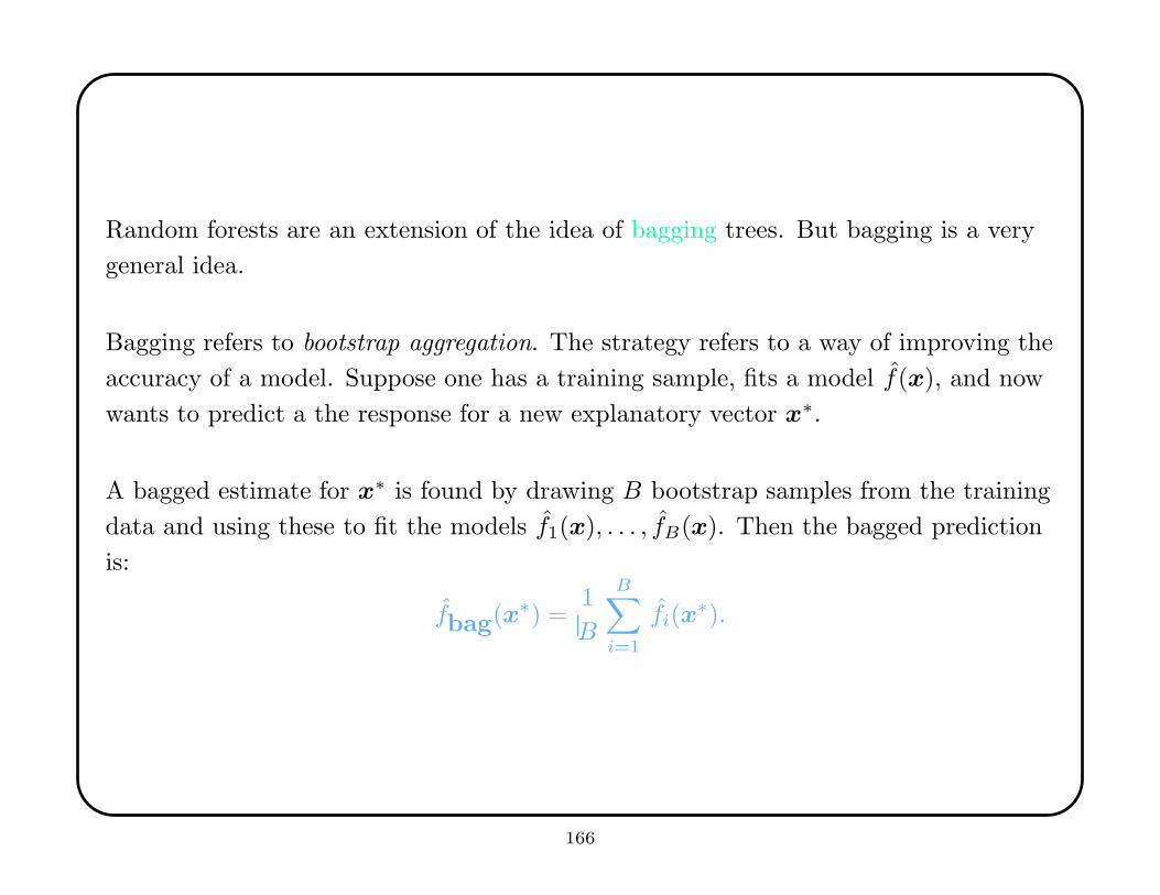
Random forests are an extension of the idea of bagging trees. But bagging is a very
general idea.
Bagging refers to bootstrap aggregation. The strategy refers to a way of improving the
accuracy of a model. Suppose one has a training sample, fits a model f(x), and now
wants to predict a the response for a new explanatory vector x∗.
A bagged estimate for x∗ is found by drawing B bootstrap samples from the training
data and using these to fit the models f1(x), . . . , fB(x). Then the bagged prediction
is:
fbag(x∗) =1
B
B∑
i=1
fi(x∗).
166

intentional blank
167
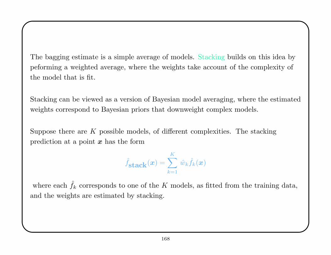
The bagging estimate is a simple average of models. Stacking builds on this idea by
peforming a weighted average, where the weights take account of the complexity of
the model that is fit.
Stacking can be viewed as a version of Bayesian model averaging, where the estimated
weights correspond to Bayesian priors that downweight complex models.
Suppose there are K possible models, of different complexities. The stacking
prediction at a point x has the form
fstack(x) =K∑
k=1
wkfk(x)
where each fk corresponds to one of the K models, as fitted from the training data,
and the weights are estimated by stacking.
168
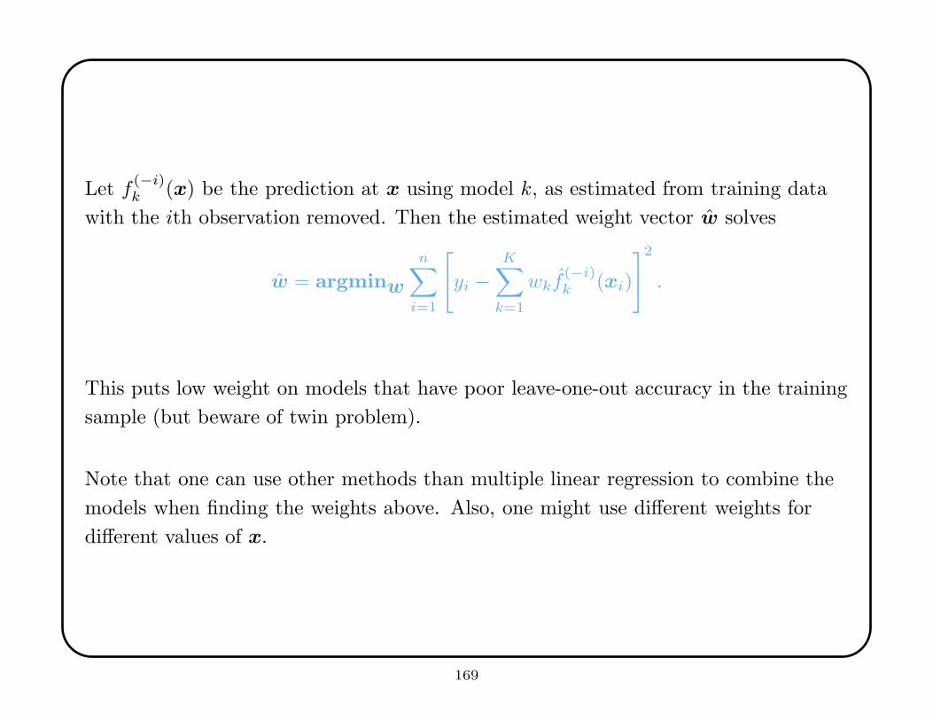
Let f(−i)k (x) be the prediction at x using model k, as estimated from training data
with the ith observation removed. Then the estimated weight vector w solves
w = argminw
n∑
i=1
[
yi −K∑
k=1
wkf(−i)k (xi)
]2
.
This puts low weight on models that have poor leave-one-out accuracy in the training
sample (but beware of twin problem).
Note that one can use other methods than multiple linear regression to combine the
models when finding the weights above. Also, one might use different weights for
different values of x.
169
7.3 Boosting
Boosting is a method invented by computer scientists to improve weak classification
rules.
If one has a classification procedure that does only slightly better than chance at
predicting the true categories, then one can apply the procedure to just the portions
of the training sample that are misclassified to produce new rules, and then weight all
the rules together to achieve better predictive accuracy. Essentially, each rule has a
weighted vote on the final classification of a case.
The procedure was proposed by Schapire (1990; Machine Learning, 5, 197-227) and
subsequently improved under the name AdaBoost. There have been many refinements
since.
170

intentional blank
171
The core algorithm for binary classification assumes one has a weak rule g1(x) that
takes values in the set {1,−1} according to the category.
AdaBoost starts by putting equal weight wi = n−1 on each of the n cases in the
training sample. Next, the algorithm repeats the following steps K times:
1. Apply the procedure gk to the training sample with weights w1, . . . , wn.
2. Find the empirical probability pw of misclassification under these weightings.
3. Calculate ck = ln (1−pw)pw
.
4. If case i is misclassified, replace wi by wi exp ck. Then renormalize so that∑n
i=1 wi = 1 and go to step 1.
The final inference is the sign of∑K
k=1 ckgk(X), which is a weighted sum of the
determinations made by each of the K rules formed from the original rule g1.
172
This boosting rule has several impressive properties:
• It provably improves classification.
• It is resistant to overfit, which arises when K is large.
• The procedure allows quick computation, and thus can be made practical even for
very large datasets.
• It can be generalized to handle more than two categories.
Boosting provides an automatic and effective way to increase the capability of almost
any classification technique.
As a new method, it is the object of active research; Friedman, Hastie, and Tibshirani
(2000; Annals of Statistics, 28, 337-407) link it to formal statistical models such as
logistic regression and generalized additive models.
173
To illustrate the power of boosting, the following graph was constructed by
Hastie, Tibshirani, and Friedman (2001; The Elements of Statistical Learning,
Springer-Verlag).
The graph shows the peformance of a “stump” (i.e., a two-node classfication tree), a
400-node classification tree, and a boosted version of the stump.
The training data are 2000 cases in X i ∈ IR10; each component is drawn
independently from a standard normal distribution. The labels are deterministically
assigned, according to:
Y =
1 if∑
X2i > 9.34
−1 if∑
X2i ≤ 9.34.
Note that the χ210 distribution has median 9.34. The test data consist of 10,000 such
values.
174

intentional blank
175

intentional blank
176
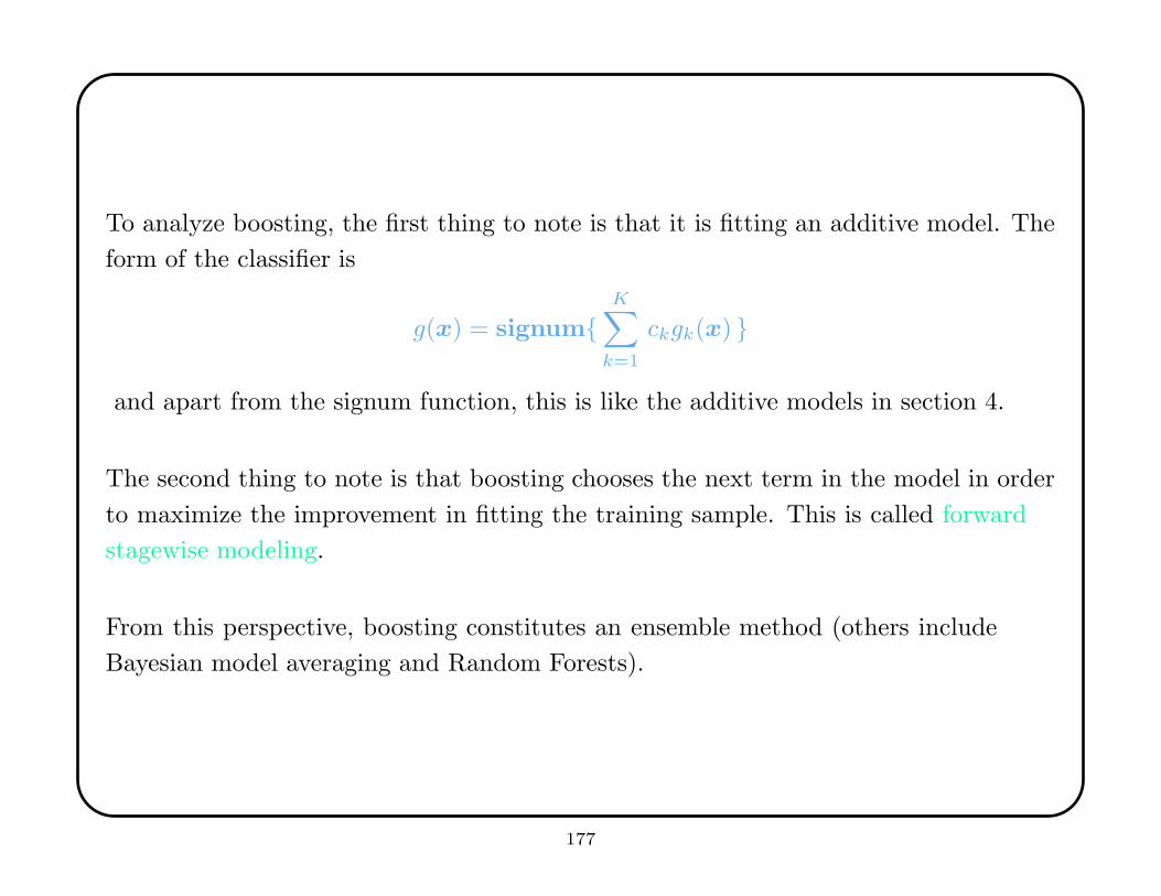
To analyze boosting, the first thing to note is that it is fitting an additive model. The
form of the classifier is
g(x) = signum{K∑
k=1
ckgk(x) }
and apart from the signum function, this is like the additive models in section 4.
The second thing to note is that boosting chooses the next term in the model in order
to maximize the improvement in fitting the training sample. This is called forward
stagewise modeling.
From this perspective, boosting constitutes an ensemble method (others include
Bayesian model averaging and Random Forests).
177
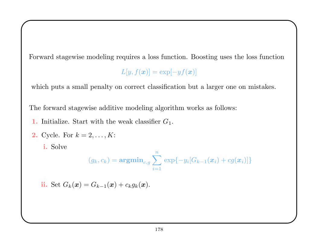
Forward stagewise modeling requires a loss function. Boosting uses the loss function
L[y, f(x)] = exp[−yf(x)]
which puts a small penalty on correct classification but a larger one on mistakes.
The forward stagewise additive modeling algorithm works as follows:
1. Initialize. Start with the weak classifier G1.
2. Cycle. For k = 2, . . . ,K:
i. Solve
(gk, ck) = argminc,g
n∑
i=1
exp{−yi[Gk−1(xi) + cg(xi)]}
ii. Set Gk(x) = Gk−1(x) + ckgk(x).
178
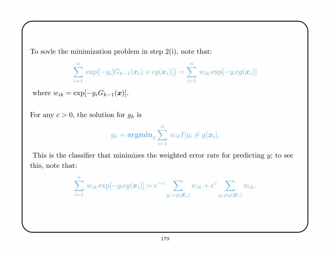
To sovle the minimization problem in step 2(i), note that:
n∑
i=1
exp{−yi[Gk−1(xi) + cg(xi)]} =n∑
i=1
wik exp[−yicg(xi)]
where wik = exp[−yiGk−1(x)].
For any c > 0, the solution for gk is
gk = argming
n∑
i=1
wikI[yi 6= g(xi].
This is the classifier that minimizes the weighted error rate for predicting y; to see
this, note that:
n∑
i=1
wik exp[−yicg(xi)] = e−c∑
yi=g(xi)
wik + ec∑
yi 6=g(xi)
wik.
179
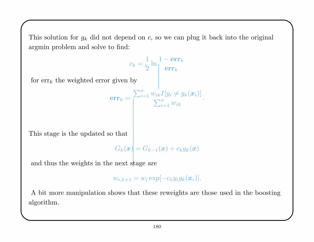
This solution for gk did not depend on c, so we can plug it back into the original
argmin problem and solve to find:
ck =1
2ln
1 − errk
errk
for errk the weighted error given by
errk =
∑ni=1 wikI[yi 6= gk(xi)]
∑ni=1 wik
.
This stage is the updated so that
Gk(x) = Gk−1(x) + ckgk(x)
and thus the weights in the next stage are
wi,k+1 = wi exp[−ckyigk(xi)].
A bit more manipulation shows that these reweights are those used in the boosting
algorithm.
180
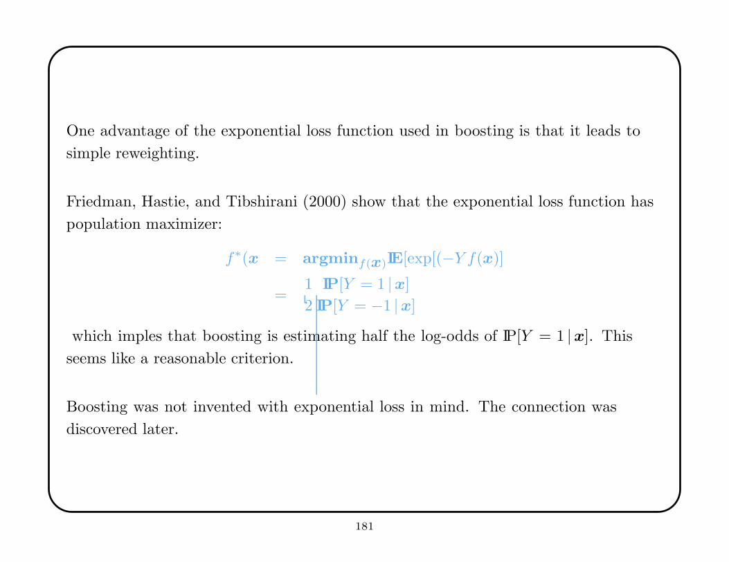
One advantage of the exponential loss function used in boosting is that it leads to
simple reweighting.
Friedman, Hastie, and Tibshirani (2000) show that the exponential loss function has
population maximizer:
f∗(x = argminf(x)IE[exp[(−Y f(x)]
=1
2
IP[Y = 1 |x]
IP[Y = −1 |x]
which imples that boosting is estimating half the log-odds of IP[Y = 1 |x]. This
seems like a reasonable criterion.
Boosting was not invented with exponential loss in mind. The connection was
discovered later.
181
8. Cluster Analysis
In data mining, cluster analysis is often called structure discovery. Traditional
data methods attempt to cluster all of the cases, but in data mining is is often
sufficient to just find some of the clusters.
Recent applications include:
• market segmentation (e.g., Claritas, Inc.)
• syndromic surveillance
• text retrieval
• microarray data
182
Classical statistics invented three kinds of cluster analysis, many of which were
independently reinvented by computer scientists. These three families are:
• hierarchical agglomerative clustering, which developed in the biological sciences
and is the most widely used strategy;
• k-means clustering, which is an algorithmic technique invented by MacQueen
(1967; Proceedings of the Fifth Berkeley Symposium on Mathematical Statistics
and Probability, University of California Press, 281-297);
• mixture models, which were recently proposed by Banfield and Raftery (1993;
Biometrics, 49, 803-821) and are gaining wide currency.
Of these three methods mixture models make the strongest assumptions about the
data being a random sample from a population, but this is also the method which
best supports inference.
183

8.1 Hierarchical Clustering
Hierarchical agglomerative clustering joins cases together according to a fixed set of
rules.
0. One starts with a sample x1, . . . ,xn of cases and a metric d on all possible sets of
cases (including the singleton sets).
1. At the first step, one joins the two cases xi and xj that have the minimum
distances among all possible pairs of cases.
2. At the second step, one joins either two singleton cases or a case xk to {xi,xj},according to whichever situation achieves minimum distance.
3. At subsequent steps one may be joining either pairs of cases, pairs of sets of cases,
or a case to a set.
Sibson and Jardine (1971; Mathematical Taxonomy, Wiley) show that this approach
uniquely satisfies certain theoretically desirable properties.
184
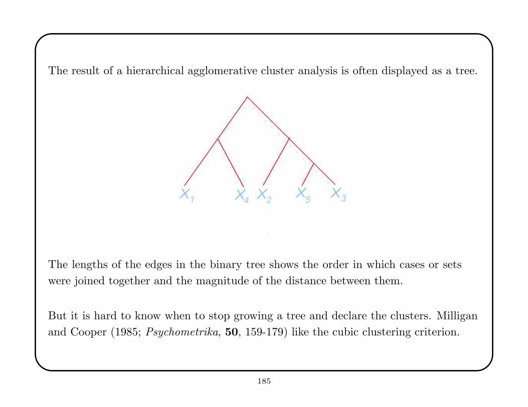
The result of a hierarchical agglomerative cluster analysis is often displayed as a tree.
The lengths of the edges in the binary tree shows the order in which cases or sets
were joined together and the magnitude of the distance between them.
But it is hard to know when to stop growing a tree and declare the clusters. Milligan
and Cooper (1985; Psychometrika, 50, 159-179) like the cubic clustering criterion.
185
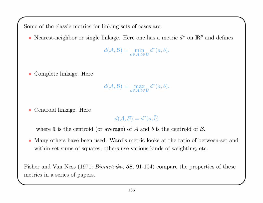
Some of the classic metrics for linking sets of cases are:
• Nearest-neighbor or single linkage. Here one has a metric d∗ on IRp and defines
d(A,B) = mina∈A,b∈B
d∗(a, b).
• Complete linkage. Here
d(A,B) = maxa∈A,b∈B
d∗(a, b).
• Centroid linkage. Here
d(A,B) = d∗(a, b)
where a is the centroid (or average) of A and b is the centroid of B.
• Many others have been used. Ward’s metric looks at the ratio of between-set and
within-set sums of squares, others use various kinds of weighting, etc.
Fisher and Van Ness (1971; Biometrika, 58, 91-104) compare the properties of these
metrics in a series of papers.
186
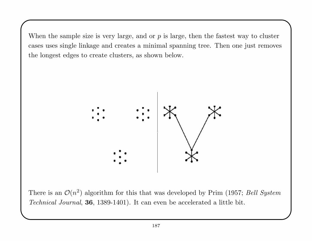
When the sample size is very large, and or p is large, then the fastest way to cluster
cases uses single linkage and creates a minimal spanning tree. Then one just removes
the longest edges to create clusters, as shown below.
There is an O(n2) algorithm for this that was developed by Prim (1957; Bell System
Technical Journal, 36, 1389-1401). It can even be accelerated a little bit.
187
When p is large and most of the measurements are noise, then it is very difficult to
discover true cluster structure. The signal that distinguishes the clusters gets lost in
the chance variation among the spurious variables.
Graphical methods such as G-Gobi take too long to find interesting projections
(via a Hermite polynomial function that measures “interestingness” according to
the “gappiness” of the projection). See Swayne, Cook, and Buja (1998; Journal of
Computational and Graphical Statistics, 7, 113-130).
Visualization techniques probably become infeasible for p > 10 or so.
188
Another thing that can happen with large p is that there are multiple cluster
structures. Here cases show strong clustering with respect to one subset of variables,
and comparably strong, but distinct, clusters with respect to a different subset of the
variables.
This situation gives rise to product structure in the clustering, which quickly becomes
unmanageable.
Friedman and Meulman (2004, Journal of the Royal Statistical Society, Series B, to
appear) discuss this problem and related issues. One strategy for visualizing multiple
cluster structure is to use parallel coordinate plots, invented by Inselberg (1985; The
Visual Computer, 1, 69-91).
189
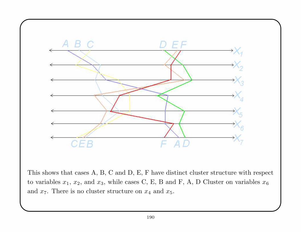
This shows that cases A, B, C and D, E, F have distinct cluster structure with respect
to variables x1, x2, and x3, while cases C, E, B and F, A, D Cluster on variables x6
and x7. There is no cluster structure on x4 and x5.
190
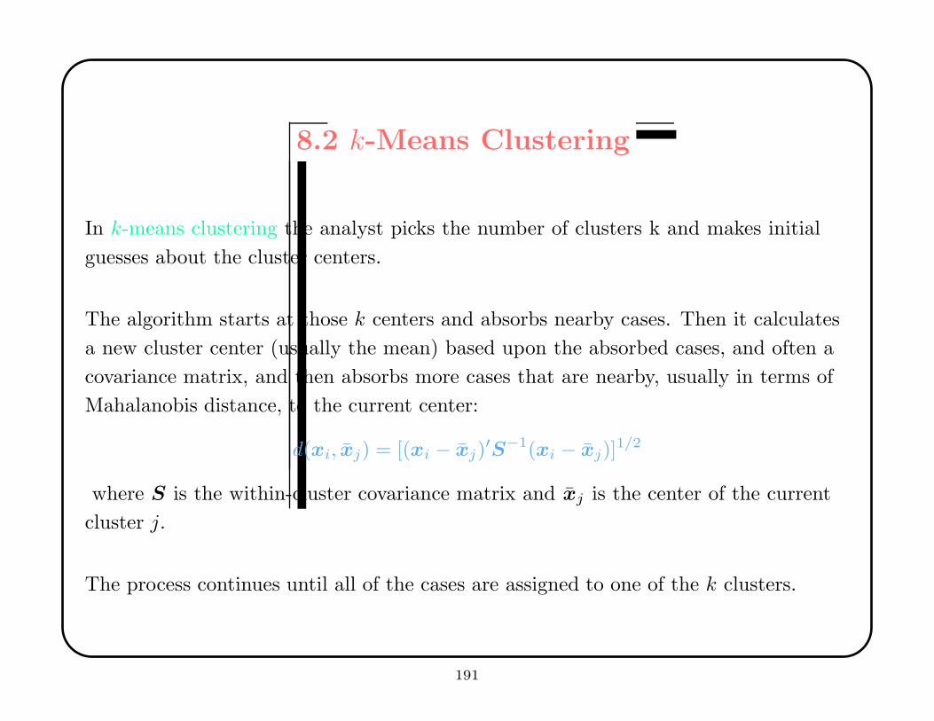
8.2 k-Means Clustering
In k-means clustering the analyst picks the number of clusters k and makes initial
guesses about the cluster centers.
The algorithm starts at those k centers and absorbs nearby cases. Then it calculates
a new cluster center (usually the mean) based upon the absorbed cases, and often a
covariance matrix, and then absorbs more cases that are nearby, usually in terms of
Mahalanobis distance, to the current center:
d(xi, xj) = [(xi − xj)′S−1(xi − xj)]
1/2
where S is the within-cluster covariance matrix and xj is the center of the current
cluster j.
The process continues until all of the cases are assigned to one of the k clusters.
191
Smart computer scientists can do k-means clustering (or approximately this) very
quickly. Andrew Moore presented methods at the NSA conference on streaming data
in December 2002.
As in hierarchical agglomerative clustering, it is hard to know k. But one can do
univariate search—try many values of k, and pick the one at the knee of some
lack-of-fit curve, e.g., the ratio of the average within-cluster to between-cluster sum of
squares.
The cluster centers move over time. If they move too much, this suggests that the
clusters are unstable.
No unique solution is guaranteed for k-means clustering. In particular, if two starting
points fall within the same true cluster, then it can be hard to discover new clusters.
192

8.2.1 Self-Organizing Maps
Kohonen (1989; Self-Organization and Associative Memory, Springer-Verlag)
developed a procedure called Self-Organizing Maps or SOMs. They quickly become
popular for visualizing complex data.
SOMs have become widely used in some aspects of business and information
technology, but their underlying theory may be weak. There is no real way to specify
uncertainty, and the method is highly susceptible to outliers.
It turns out that SOMs can be viewed as k-means clustering with the constraint that
the cluster centers have to lie in a plane.
193
SOMs are rather like multidimensional scaling. The intention is to produce a
two-dimensional (sometimes three-dimensional) picture of high-dimensional data, one
that puts similar observations close together in the visualization.
One starts with a set of prototypes, which are just the integer coordinates in the
plane formed by the first two principal components of the data. This plane is then
distorted, so as to pull the prototypes near to the data. Finally, the data are identified
with their nearest point on the distorted surface.
The following two examples of SOMs are heatmaps showing the number of documents
in the newsgroup corpus comp.ai.neural-nets with different kinds of subject
matter, taken from the WEBSOM homepage. The first is the entire corpus (with
well-populated nodes tagged with their keyword), and the second is a blow-up of the
heatmap focused on the region around “mining”.
194
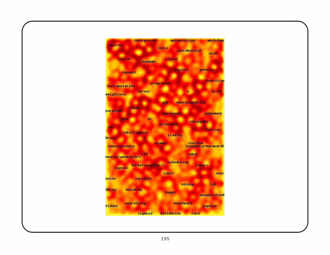
195
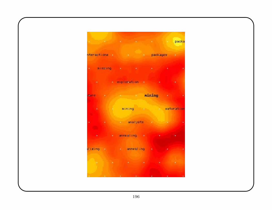
196
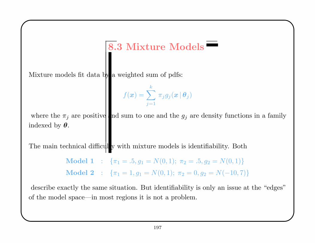
8.3 Mixture Models
Mixture models fit data by a weighted sum of pdfs:
f(x) =k∑
j=1
πjgj(x |θj)
where the πj are positive and sum to one and the gj are density functions in a family
indexed by θ.
The main technical difficulty with mixture models is identifiability. Both
Model 1 : {π1 = .5, g1 = N(0, 1); π2 = .5, g2 = N(0, 1)}Model 2 : {π1 = 1, g1 = N(0, 1); π2 = 0, g2 = N(−10, 7)}
describe exactly the same situation. But identifiability is only an issue at the “edges”
of the model space—in most regions it is not a problem.
197
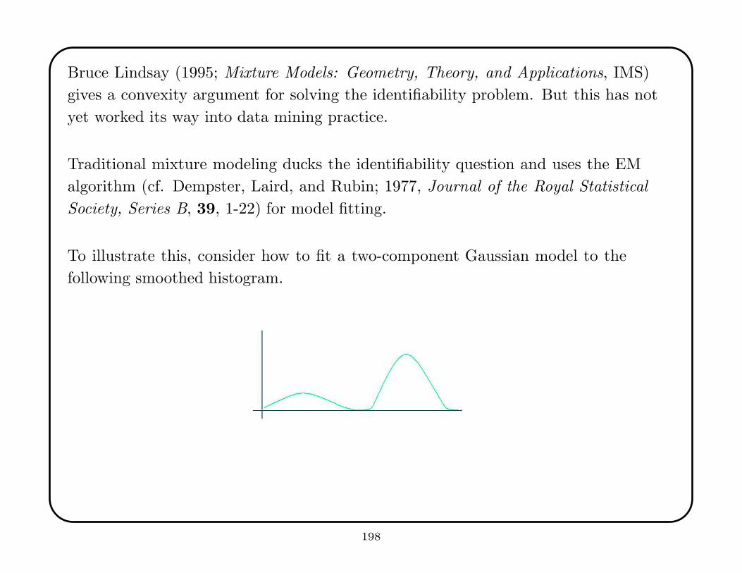
Bruce Lindsay (1995; Mixture Models: Geometry, Theory, and Applications, IMS)
gives a convexity argument for solving the identifiability problem. But this has not
yet worked its way into data mining practice.
Traditional mixture modeling ducks the identifiability question and uses the EM
algorithm (cf. Dempster, Laird, and Rubin; 1977, Journal of the Royal Statistical
Society, Series B, 39, 1-22) for model fitting.
To illustrate this, consider how to fit a two-component Gaussian model to the
following smoothed histogram.
198
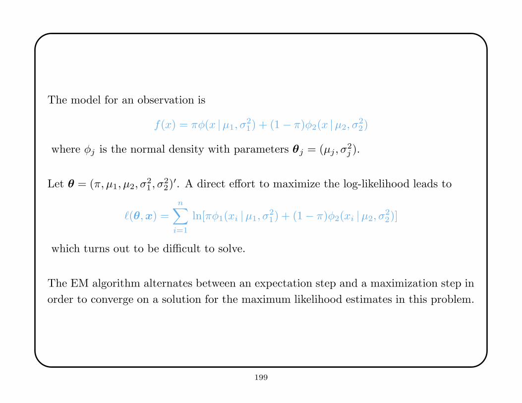
The model for an observation is
f(x) = πφ(x |µ1, σ21) + (1 − π)φ2(x |µ2, σ
22)
where φj is the normal density with parameters θj = (µj , σ2j ).
Let θ = (π, µ1, µ2, σ21 , σ
22)
′. A direct effort to maximize the log-likelihood leads to
`(θ,x) =n∑
i=1
ln[πφ1(xi |µ1, σ21) + (1 − π)φ2(xi |µ2, σ
22)]
which turns out to be difficult to solve.
The EM algorithm alternates between an expectation step and a maximization step in
order to converge on a solution for the maximum likelihood estimates in this problem.
199
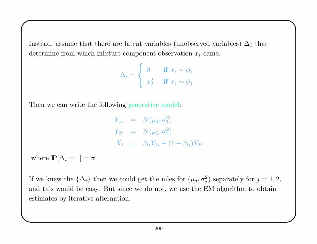
Instead, assume that there are latent variables (unobserved variables) ∆i that
determine from which mixture component observation xi came.
∆i =
0 if xi ∼ φ2
x22 if xi ∼ φ1
Then we can write the following generative model:
Y1i = N(µ1, σ21)
Y2i = N(µ2, σ22)
Xi = ∆iY1i + (1 − ∆i)Y2i
where IP[∆i = 1] = π.
If we knew the {∆i} then we could get the mles for (µj , σ2j ) separately for j = 1, 2,
and this would be easy. But since we do not, we use the EM algorithm to obtain
estimates by iterative alternation.
200
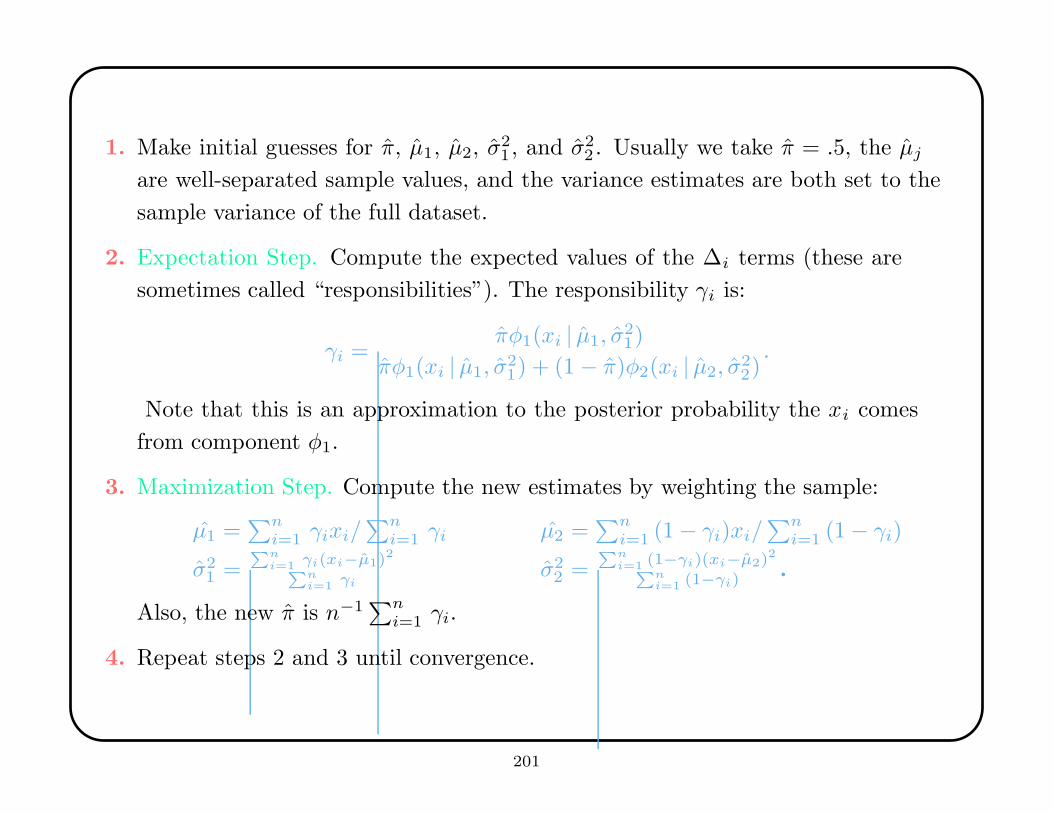
1. Make initial guesses for π, µ1, µ2, σ21 , and σ2
2 . Usually we take π = .5, the µj
are well-separated sample values, and the variance estimates are both set to the
sample variance of the full dataset.
2. Expectation Step. Compute the expected values of the ∆i terms (these are
sometimes called “responsibilities”). The responsibility γi is:
γi =πφ1(xi | µ1, σ
21)
πφ1(xi | µ1, σ21) + (1 − π)φ2(xi | µ2, σ2
2).
Note that this is an approximation to the posterior probability the xi comes
from component φ1.
3. Maximization Step. Compute the new estimates by weighting the sample:
µ1 =∑n
i=1 γixi/∑n
i=1 γi µ2 =∑n
i=1 (1 − γi)xi/∑n
i=1 (1 − γi)
σ21 =
P
ni=1
γi(xi−µ1)2
P
ni=1
γiσ2
2 =P
ni=1
(1−γi)(xi−µ2)2
P
ni=1
(1−γi).
Also, the new π is n−1∑n
i=1 γi.
4. Repeat steps 2 and 3 until convergence.
201

intentional blank
202
The EM algorithm climbs hills, so in general it converges to a local (but possibly not
global) maximum. In part, it is fast because it increases the criterion function on both
steps, not just the maximization step.
The EM algorithm does not solve the identifiability problem that can arise in mixture
models. But it does find a local mle.
The EM algorithm is considerably more flexible than this example indicates, and
it applies in a wide variety of cases (e.g., imputation in missing data problems,
inference on causation through counterfactual data). The review given here follows
the application in Hastie, Tibshirani, and Friedman (2001; The Elements of Statistical
Learning, Wiley, chap. 8.5).
203
8.3.1 Model-Based Cluster Analysis
This is a parametric family of mixture models (usually Gaussian mixtures) that are
becoming widely used in both cluster analysis and data mining.
Essentially, this uses a nested sequence of normal mixtures for cluster analysis. The
nesting enables one to use likelihood ratio tests to determine which level of modeling
is appropriate.
1. At the most nested level, the model assumes that the data come from a
k-component mixture of normal distributions, each with a common covariance
matrix but different means.
2. At the next-most nested level, the covariance matrices are allowed to differ by an
unknown scalar multiple.
3. At the highest level, the covariance matrices for different components are
completely unrelated.
204
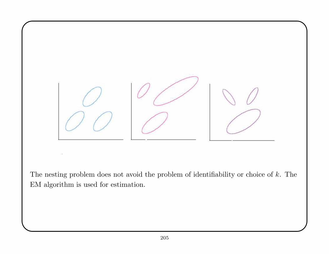
The nesting problem does not avoid the problem of identifiability or choice of k. The
EM algorithm is used for estimation.
205
9. Issues with Bases
Nonparametric regression often tries to fit a model of the form
f(x) =M∑
j=1
βjhj(x) + ε
where the hj functions may pick out specific components of x (multiple linear
regression), or be powers of components of x (polynomial regression), or be
prespecified transformations of components of x (nonlinear regression).
Many functions f cannot be represented by the kinds of hj listed above. But if the
set {hj} is an orthogonal basis for a space of functions that contains f , then we can
exploit many standard strategies from linear regression.
206
9.1 Hilbert Spaces
Usually we are concerned with spaces of functions such as L2[a, b], the Hilbert space
of all real-valued functions defined on the interval [a, b] that are square-integrable:
∫ b
a
f(x) dx <∞.
This definition extends to functions on IRp.
Hilbert spaces have an inner product. For L2[a, b] it is
< f, g >=
∫ b
a
f(x)g(x) dx.
The inner product defines a norm ‖f‖, given by < f, g >1/2, which is essentially a
metric on the space of functions.
There are additional issues for a Hilbert space, such as completeness (i.e., the space
contains the limit of all Cauchy sequences), but we can ignore those.
207
A set of functions {hj} in a Hilbert space is mutually orthogonal if for all j 6= k,
< hj , hk >= 0.
Additionally, if ‖hj‖ = 1 for all j, then the set is orthonormal.
If {hj} is an orthonormal basis for a space H then every function f ∈ H can be
uniquely written as:
f(x) =
∞∑
j=1
βjhj(x)
where
βj =< f, hj > .
Some famous orthogonal bases include the Fourier bases, consisting of {cosnx, sinnx},wavelets, Legendre polynomials, and Hermite polynomials.
208
If one has an orthonormal basis for the space in which f lives, then several nice things
happen:
1. Since f is a linear function of the basis elements, then simple regression methods
allow us to estimate the coefficients βj .
2. Since the basis is orthogonal, the estimates of different βj coefficients are
independent.
3. Since the set is a basis, there is no identifiability problem; each function in H is
uniquely expressed as a weighted sum of basis elements.
But not all orthonormal bases are equally good. If one can find a basis that includes
f itself, that would be ideal. Second best is a basis in which only a few elements in
the representation of f have non-zero coefficients. But this problem is tautological
since we do not know f .
209
One approach to choosing a basis is to use Gram-Schmidt orthogonalization to
construct a basis set such that the first few elements correspond to the kinds of
functions that statisticians expect to encounter.
This approach is often practical if the right kind of domain knowledge is available.
This is often the case in audio signal processing; Fourier series are natural ways to
represent vibration.
But in general, one must pick basis set without regard to f . A common criterion is
that the influence of the basis elements be local. From this standpoint, polynomials
and trigonometric functions are bad, because their support is the whole line, but
splines and wavelets are good, because their support is essentially compact.
210
Given an orthonormal basis, one can try estimating all of the {βj}. But one quickly
runs out of data—even if f is exactly equal to one of the basis elements, noise ensures
that all of the other elements will make some contribution to the fit.
To address this problem one can:
• Restrict the set of functions, so it is no longer a basis (e.g., linear regression);
• select only those basis elements that seem to contribute significantly to the fit of
the model (e.g., variable selection methods, or greedy fitters like MARS, CART,
and boosting);
• regularize, to restrict the values of the coefficients (e.g., through ridge regression
or shrinkage or thesholding).
The first technique is problematic, especially since it prevents flexibility in fitting
nonlinear functions.
The second technique is important, especially when one has large p but small n.
But it is often insufficient, and the theory for aggressive variable selection is not
well-developed yet.
211
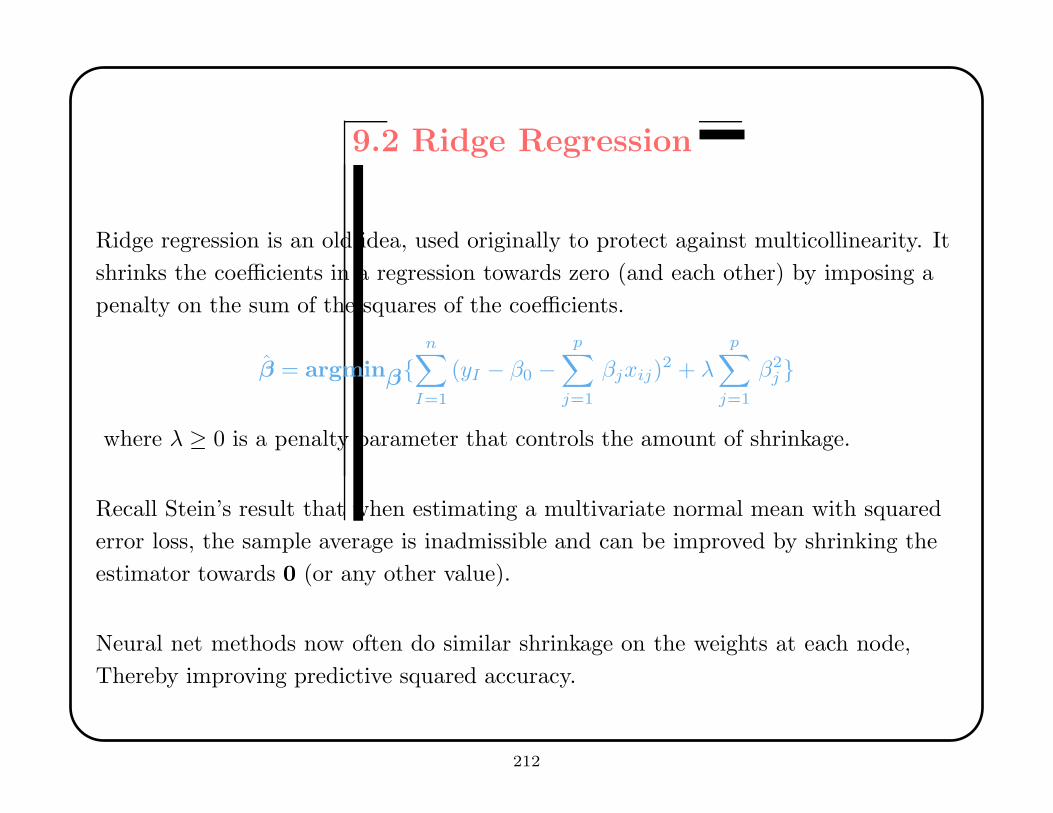
9.2 Ridge Regression
Ridge regression is an old idea, used originally to protect against multicollinearity. It
shrinks the coefficients in a regression towards zero (and each other) by imposing a
penalty on the sum of the squares of the coefficients.
β = argminβ{n∑
I=1
(yI − β0 −p∑
j=1
βjxij)2 + λ
p∑
j=1
β2j }
where λ ≥ 0 is a penalty parameter that controls the amount of shrinkage.
Recall Stein’s result that when estimating a multivariate normal mean with squared
error loss, the sample average is inadmissible and can be improved by shrinking the
estimator towards 0 (or any other value).
Neural net methods now often do similar shrinkage on the weights at each node,
Thereby improving predictive squared accuracy.
212

intentional blank
213
Ridge regression methods are not equivariant under scaling, so one normally
standardizes the xij sample values wrt j so that each has unit variance.
Traditional ridge regression solves
β = (X ′X + λI)−1X ′y
so the name derives from the stabilization of the inverse matrix obtained by adding a
constant to the diagonal.
Note that this increases the trace of the hat matrix, which corresponds to the degrees
of freedom used in fitting the model.
Ridge regression (and shrinkage methods in general) can be obtained as the Bayesian
posterior mode for a suitable prior. In the multivariate normal case, the prior assumes
independent normal distributions for each βj , with common variance.
214

intentional blank
215
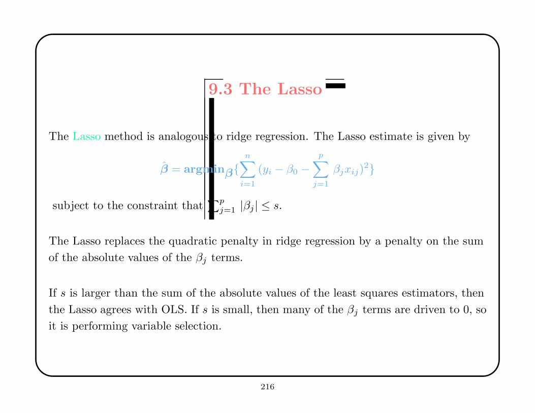
9.3 The Lasso
The Lasso method is analogous to ridge regression. The Lasso estimate is given by
β = argminβ{n∑
i=1
(yi − β0 −p∑
j=1
βjxij)2}
subject to the constraint that∑p
j=1 |βj | ≤ s.
The Lasso replaces the quadratic penalty in ridge regression by a penalty on the sum
of the absolute values of the βj terms.
If s is larger than the sum of the absolute values of the least squares estimators, then
the Lasso agrees with OLS. If s is small, then many of the βj terms are driven to 0, so
it is performing variable selection.
216
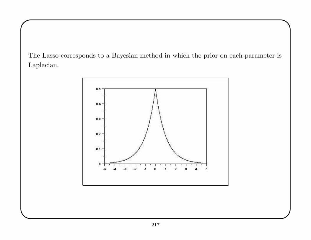
The Lasso corresponds to a Bayesian method in which the prior on each parameter is
Laplacian.
217
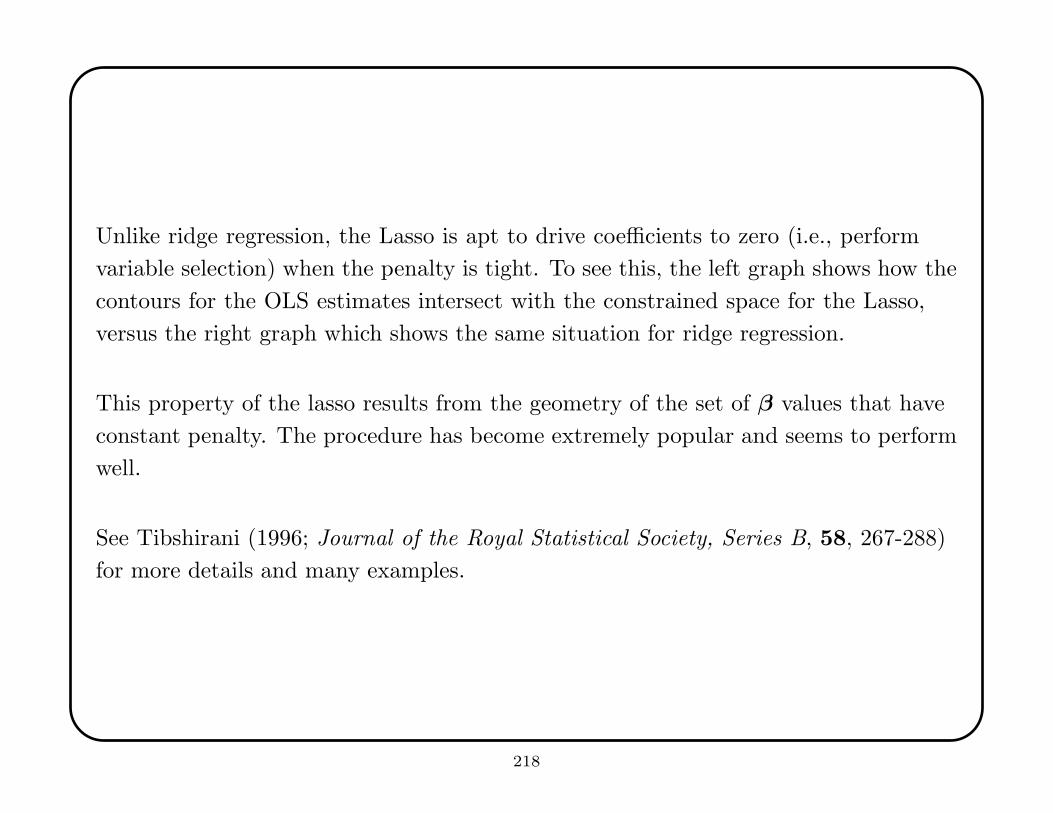
Unlike ridge regression, the Lasso is apt to drive coefficients to zero (i.e., perform
variable selection) when the penalty is tight. To see this, the left graph shows how the
contours for the OLS estimates intersect with the constrained space for the Lasso,
versus the right graph which shows the same situation for ridge regression.
This property of the lasso results from the geometry of the set of β values that have
constant penalty. The procedure has become extremely popular and seems to perform
well.
See Tibshirani (1996; Journal of the Royal Statistical Society, Series B, 58, 267-288)
for more details and many examples.
218

intentional blank
219
intentional blank
220

intentional blank
221

intentional blank
222
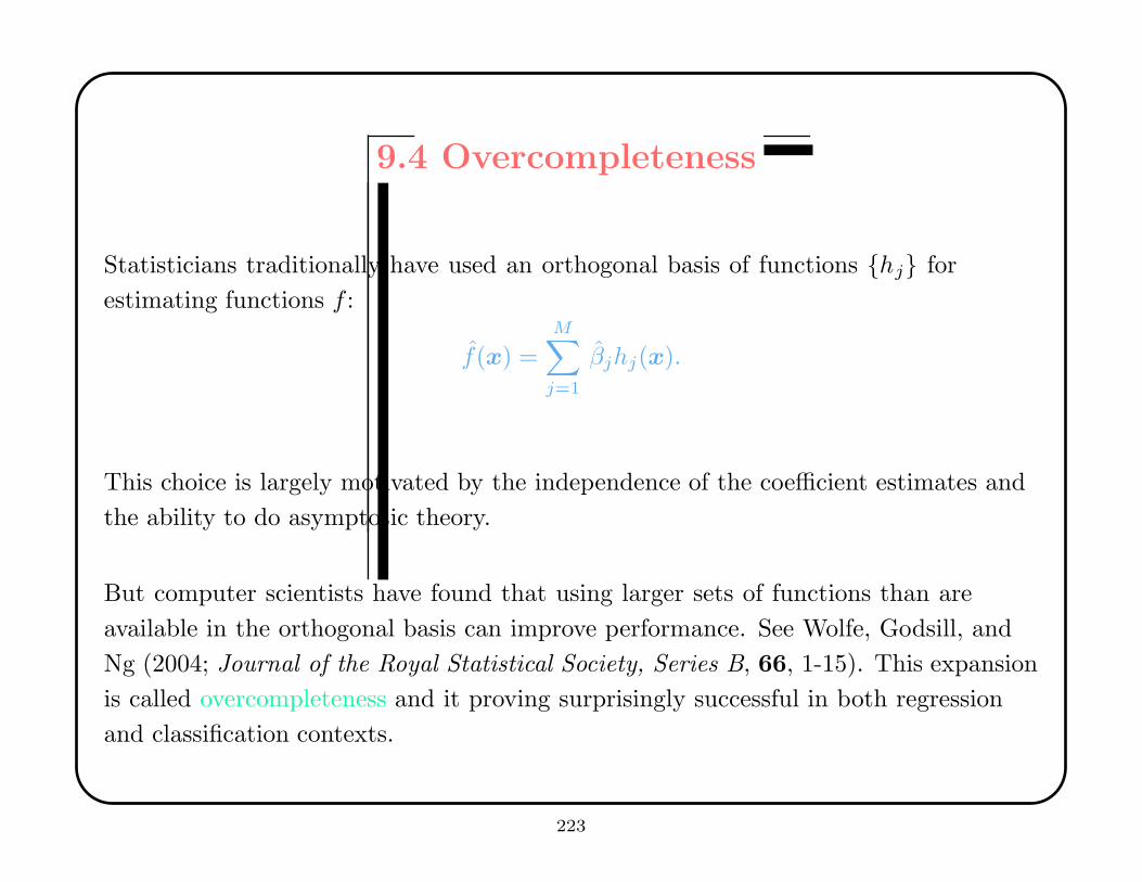
9.4 Overcompleteness
Statisticians traditionally have used an orthogonal basis of functions {hj} for
estimating functions f :
f(x) =M∑
j=1
βjhj(x).
This choice is largely motivated by the independence of the coefficient estimates and
the ability to do asymptotic theory.
But computer scientists have found that using larger sets of functions than are
available in the orthogonal basis can improve performance. See Wolfe, Godsill, and
Ng (2004; Journal of the Royal Statistical Society, Series B, 66, 1-15). This expansion
is called overcompleteness and it proving surprisingly successful in both regression
and classification contexts.
223
This larger set is called a frame. A frame contains a basis for the space of interest
(e.g., L2[a, b]), but may also other functions. Formally, a frame is a set of functions
{hj : j ∈ J} with the property that there are constants A,B > 0 such that
A‖f‖2 ≤∑
j∈J
| < f, hj > |2 ≤ B‖f‖2 ∀f ∈ H.
A frame that is just an ordinary basis has A = B = 1. A frame that is the union of
two ordinary bases has A = B = 2. Some frames have uncountable cardinality.
Nontrivial frames contain at least one non-zero element which can be written as
a linear combination of the other elements in the frame. This contrasts with the
situation for basis sets.
The advantage of frames is that their greater size allows the possibility of finding a
very parsimonious representation for f .
224
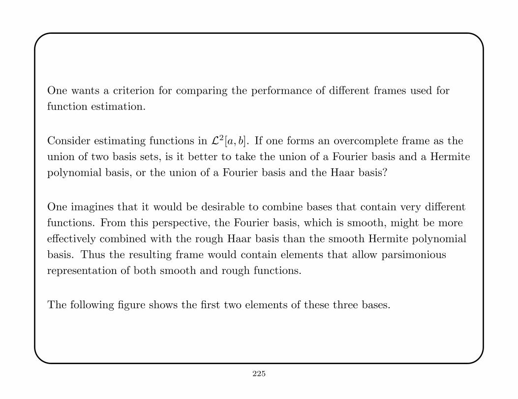
One wants a criterion for comparing the performance of different frames used for
function estimation.
Consider estimating functions in L2[a, b]. If one forms an overcomplete frame as the
union of two basis sets, is it better to take the union of a Fourier basis and a Hermite
polynomial basis, or the union of a Fourier basis and the Haar basis?
One imagines that it would be desirable to combine bases that contain very different
functions. From this perspective, the Fourier basis, which is smooth, might be more
effectively combined with the rough Haar basis than the smooth Hermite polynomial
basis. Thus the resulting frame would contain elements that allow parsimonious
representation of both smooth and rough functions.
The following figure shows the first two elements of these three bases.
225
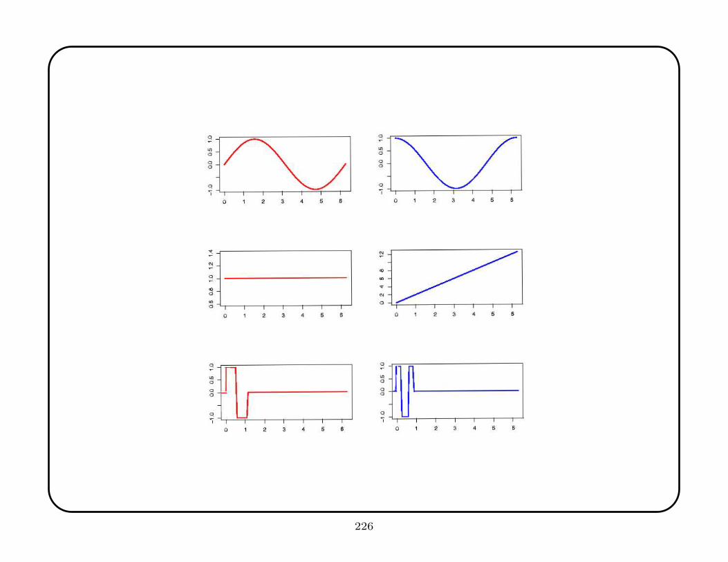
226
One proposal for a criterion that compares two frames depends upon the parsimony
of the approximating functions.
For a given frame F = {hj : j ∈ J }, a function f , and a tolerance ε∗, consider the set
of all approximating functions
S(f, ε∗) = { f : f =
k∑
j=1
βjhj and ‖f − f‖ < ε∗ }.
Each f ∈ S(f, ε∗) has a certain number of terms in the sum. The most parsimonious
approximation is the one that uses the fewest terms hj . Let
k(f, ε∗) = inf{j : f ∈ S(f, ε∗)}.
Some functions f ∈ L2[0, 1] will be hard to approximate with elements in the frame
F , and for these functions k(f, ε∗) will be large (and maybe infinite).
227
To handle the worst case for estimation, let
k(ε∗) = supf∈L2[0,1]
{ k(f, ε∗) }.
This is the number of terms needed to approximate the most difficult function in
L2[0, 1] to within ε∗ using only frame elements.
For some frames and values ε∗, k(ε∗) will be infinite. But there are many cases in
which it is finite. For example, if F contains an ε∗-net, this trivially ensures that
k(ε∗) = 1.
For non-trivial cases in which frames F and G are unions of bases, one would like to
say that frame F is better than frame G at level ε∗ if kF (ε∗) < kG(ε∗), where the
subscript indicates the frame.
If there exists some γ such that the inequality holds for all ε∗ < γ, then one could
broadly claim that F is better than G.
228
10. Wavelets
A wavelet is a function that looks like a localized wiggle. Special collections of
wavelets can be used to obtain approximations of functions by separating then
information at different scales.
The stunning success of wavelets has spurred explosive growth in research. Donoho
and Johnstone (1994; Biometrika, 81, 425-455) led the way in statistics, showing that
wavelets can achieve local asymptotic minimaxity in approximating thick classes of
functions.
Local asymptotic minimaxity is a technical property, but it ensures that the estimates
are asymptotically minimax with respect to a large family of loss functions in a large
class of functions. Such estimates probably evade the COD, in the same technical
sense that neural nets do.
229
In its simplest form, a wavelet representation begins with a single function ψ, often
called th mother wavelet.
We define a collection of wavelets—called a wavelet basis—by dilation and translation
of the mother wavelet ψ:
ψjk(t) = 2j/2ψ(2jt− k)
for j, k ∈ Z, the set of integers.
One obtains an overcomplete frame if one allows j, k to take values in IR rather than
Z. This is called an undecimated wavelet basis.
Each ψjk has a characteristic resolution scale (determined by j) and is roughly
centered on the location k/2j . It turns out that if ψ is properly chosen, any
“reasonable” function can be represented by an infinite linear combination of the ψjk
functions.
230
Wavelets have three key features:
• Wavelets provide sparse representations of a broad class of functions and signals,
• Wavelets can achieve very good localization in both time and frequency,
• There are fast algorithms for computing wavelet representations in practice.
Sparsity means that most of coefficients in the linear combination are nearly zero. A
single wavelet basis can provide sparse representations of many spaces of functions at
the same time.
Good localization means that both the wavelet function ψ and its Fourier transform
have small support; i.e., the functions are essentially zero outside some compact
domain.
Regarding speed, wavelet representations can be computed in O(n log n) and
sometimes O(n) operations (the FFT is O(n logn)).
231
10.1 Constructing Wavelets
We begin with a mathematical description of a smooth localized wiggle.
Let Lp(IR) denote the space of measurable complex-valued functions f on the real
numbers IR such that
‖f‖p =
[∫
|f(x)|p]1/p
dx <∞.
Here L2(IR) is a Hilbert space with inner product defined by
< f, g >=
∫
f(x)g(x) dx,
where g is the complex conjugate of g.
Recall that a complex function g(x) = u(x) + iv(x) has conjugate g(x) = u(x) − iv(x)
where u(x) and v(x) are real-valued functions and i is√−1. The modulus of g(x) is
√
u2(x) + v2(x).
232
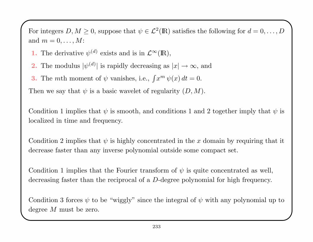
For integers D,M ≥ 0, suppose that ψ ∈ L2(IR) satisfies the following for d = 0, . . . , D
and m = 0, . . . ,M :
1. The derivative ψ(d) exists and is in L∞(IR),
2. The modulus |ψ(d)| is rapidly decreasing as |x| → ∞, and
3. The mth moment of ψ vanishes, i.e.,∫
xm ψ(x) dt = 0.
Then we say that ψ is a basic wavelet of regularity (D,M).
Condition 1 implies that ψ is smooth, and conditions 1 and 2 together imply that ψ is
localized in time and frequency.
Condition 2 implies that ψ is highly concentrated in the x domain by requiring that it
decrease faster than any inverse polynomial outside some compact set.
Condition 1 implies that the Fourier transform of ψ is quite concentrated as well,
decreasing faster than the reciprocal of a D-degree polynomial for high frequency.
Condition 3 forces ψ to be “wiggly” since the integral of ψ with any polynomial up to
degree M must be zero.
233
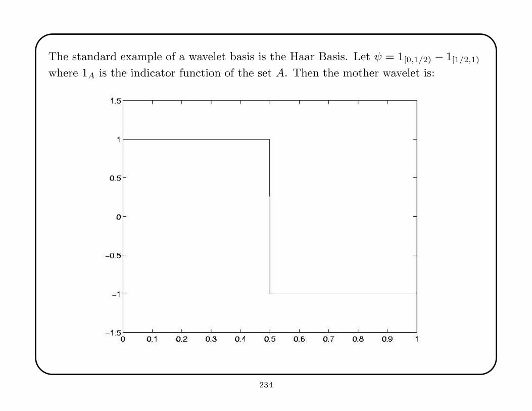
The standard example of a wavelet basis is the Haar Basis. Let ψ = 1[0,1/2) − 1[1/2,1)
where 1A is the indicator function of the set A. Then the mother wavelet is:
234
This function is not differentiable, but it has compact support and integrates any
constant to zero. Thus ψ is a basic wavelet of regularity (0, 0).
If we define ψjk from ψ by translation and dilation, we obtain a doubly-infinite set of
functions with the same properties as ψ.
Moreover, any two ψjk are orthonormal in the sense that < ψj,k, ψj′,k′ >= δjj′δkk′
where δ is a Kronecker delta.
These ψjk form an orthonormal basis for L2(IR). any function in L2(IR) can be
well-approximated by∑
j,k βj,kψjk. (As a first step in seeing this, note that it is
sufficient to be able to approximate any function that is piecewise constant on dyadic
intervals.)
235
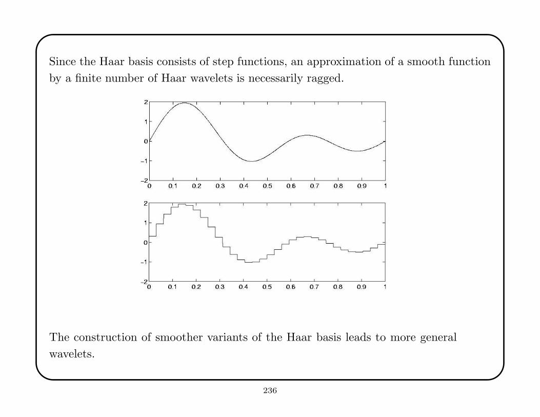
Since the Haar basis consists of step functions, an approximation of a smooth function
by a finite number of Haar wavelets is necessarily ragged.
The construction of smoother variants of the Haar basis leads to more general
wavelets.
236
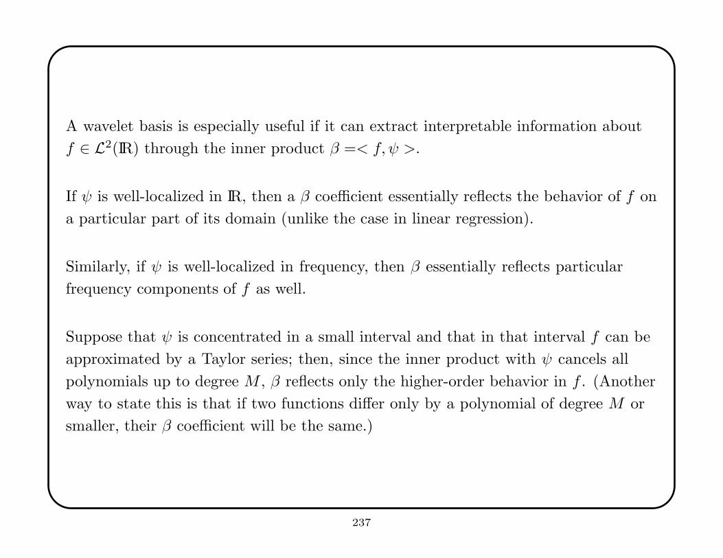
A wavelet basis is especially useful if it can extract interpretable information about
f ∈ L2(IR) through the inner product β =< f, ψ >.
If ψ is well-localized in IR, then a β coefficient essentially reflects the behavior of f on
a particular part of its domain (unlike the case in linear regression).
Similarly, if ψ is well-localized in frequency, then β essentially reflects particular
frequency components of f as well.
Suppose that ψ is concentrated in a small interval and that in that interval f can be
approximated by a Taylor series; then, since the inner product with ψ cancels all
polynomials up to degree M , β reflects only the higher-order behavior in f . (Another
way to state this is that if two functions differ only by a polynomial of degree M or
smaller, their β coefficient will be the same.)
237
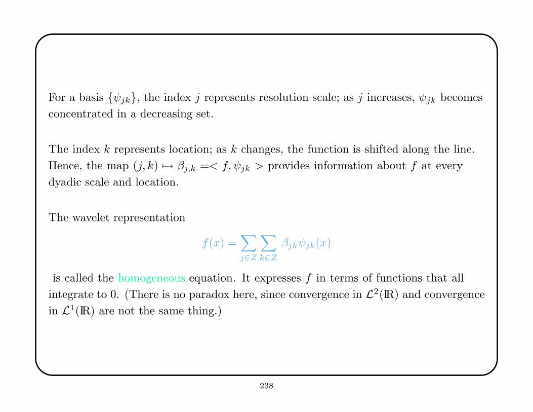
For a basis {ψjk}, the index j represents resolution scale; as j increases, ψjk becomes
concentrated in a decreasing set.
The index k represents location; as k changes, the function is shifted along the line.
Hence, the map (j, k) 7→ βj,k =< f, ψjk > provides information about f at every
dyadic scale and location.
The wavelet representation
f(x) =∑
j∈Z
∑
k∈Z
βjkψjk(x)
is called the homogeneous equation. It expresses f in terms of functions that all
integrate to 0. (There is no paradox here, since convergence in L2(IR) and convergence
in L1(IR) are not the same thing.)
238

10.2 The Father Wavelet
It is often useful to re-express the homogeneous equation in an equivalent but
inhomogeneous form. This form separates “coarse” structure from “fine” structure.
To do this, select a convenient resolution level J0. Resolution levels j ≤ J0 capture
the coarse structure of f and levels j > J0 capture the fine structure.
One approximates the fine-resolution structure of f by a linear combination of the
ψjk at j ≥ J0, and one approximates the coarse-resolution structure by a combination
of the functions φk(t) = φ(t− k) for k ∈ Z, where φ is called the father wavelet(or
scaling function).
The inhomogeneous representation for f ∈ L2(IR) is then
f =∑
k ∈Z
< f, φk > φk +∑
j≥J0
∑
k ∈Z
< f, ψjk > ψjk.
239
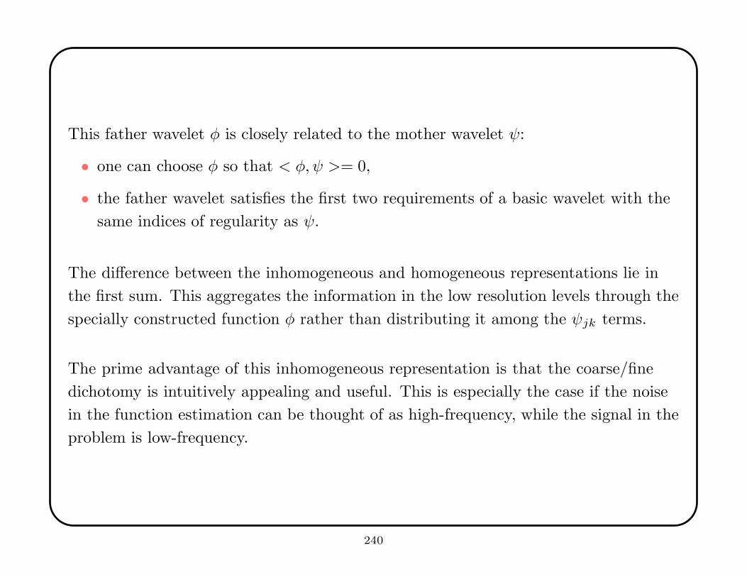
This father wavelet φ is closely related to the mother wavelet ψ:
• one can choose φ so that < φ,ψ >= 0,
• the father wavelet satisfies the first two requirements of a basic wavelet with the
same indices of regularity as ψ.
The difference between the inhomogeneous and homogeneous representations lie in
the first sum. This aggregates the information in the low resolution levels through the
specially constructed function φ rather than distributing it among the ψjk terms.
The prime advantage of this inhomogeneous representation is that the coarse/fine
dichotomy is intuitively appealing and useful. This is especially the case if the noise
in the function estimation can be thought of as high-frequency, while the signal in the
problem is low-frequency.
240
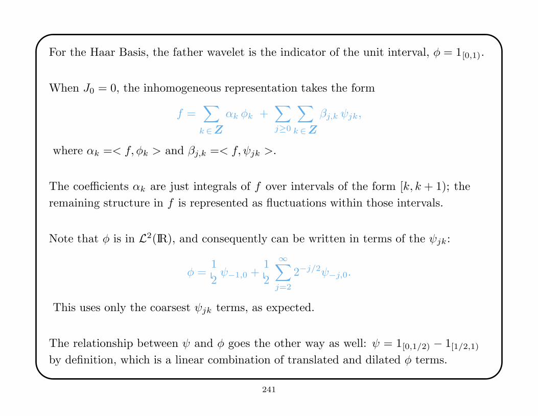
For the Haar Basis, the father wavelet is the indicator of the unit interval, φ = 1[0,1).
When J0 = 0, the inhomogeneous representation takes the form
f =∑
k ∈Z
αk φk +∑
j≥0
∑
k ∈Z
βj,k ψjk,
where αk =< f, φk > and βj,k =< f, ψjk >.
The coefficients αk are just integrals of f over intervals of the form [k, k + 1); the
remaining structure in f is represented as fluctuations within those intervals.
Note that φ is in L2(IR), and consequently can be written in terms of the ψjk:
φ =1
2ψ−1,0 +
1
2
∞∑
j=2
2−j/2ψ−j,0.
This uses only the coarsest ψjk terms, as expected.
The relationship between ψ and φ goes the other way as well: ψ = 1[0,1/2) − 1[1/2,1)
by definition, which is a linear combination of translated and dilated φ terms.
241
10.3 Multiresolution Analysis
A key idea in wavelets is that of successive refinement. If one can approximate at
several levels of accuracy, then the differences between successive approximations
characterize the refinements needed to move from one level to another.
Multiresolution analysis (MRA) formalizes this notion for approximations that are
related by a translation and dilation. An MRA is a sequence of nested approximation
spaces for a containing class of functions.
For the containing class L2(IR), MRA is a nested sequence of closed subspaces
· · · ⊂ V−2 ⊂ V−1 ⊂ V0 ⊂ V1 ⊂ V2 ⊂ · · ·
such that
1. clos{
⋃
j ∈Z Vj
}
= L2(IR) 3. f ∈ Vj ⇔ f(2−j ·) ∈ V0 ∀ j ∈ Z
2.⋂
j ∈Z Vj = {0} 4. f ∈ V0 ⇔ f(· − k) ∈ V0 ∀ k ∈ Z.
242
Condition 1 ensures that the approximation spaces (Vj) are sufficient to approximate
any function in L2(IR).
There are many sequences of spaces satisfying Conditions 1, 2 and 4; the name
“multiresolution” is derived from Condition 3 which implies that all the Vj are
dyadically scaled versions of a common space V0. By Condition 4, V0 is invariant
under integer translations.
When generating orthonormal wavelet bases, we also require that the space V0 of
the MRA contains a function φ such that the integer translations {φ0,n} form
an orthonormal basis for V0. For simplicity, we will focus almost exclusively on
orthonormal bases here.
243
Since V0 ⊂ V1, we can define its orthogonal complement W0 in V1, so V1 = V0 ⊕W0.
We can do likewise for every j, where Vj+1 = Vj ⊕Wj .
The sequence of spaces {Wj}j∈Z are mutually orthogonal and they are inherit
Condition 3 from the Vj ; i.e., f ∈Wj if and only if f(2−j ·) ∈W0.
By themselves, these spaces provide a homogeneous representation of L2(IR), since
L2(IR) = clos{∪j ∈Z Wj}. The Wj are the building blocks for successive refinement
from one approximating space to another.
Given f ∈ L2(IR), the best approximation to f in any Vj is given by Pjf , where Pj is
the orthogonal projection onto Vj . It follows that Qj = Pj − Pj−1 is the orthogonal
projection onto Wj .
244
Given a coarse approximation P0f , one can refine to the finer approximation PJf for
any J > 0 by adding details from successive Wj spaces:
PJf = P0f +
J∑
j=1
Pjf − Pj−1f
= P0f +
J−1∑
j=0
Qjf,
and as J → ∞,
f = P0f +∞∑
j=0
Qjf.
Successive refinement exactly mimics the inhomogeneous wavelet representation. The
coarse approximation P0f corresponds to a linear combination of the φ0,k, and each
Qjf for j ≥ 0 corresponds to a linear combination of the span of the ψjk.
245
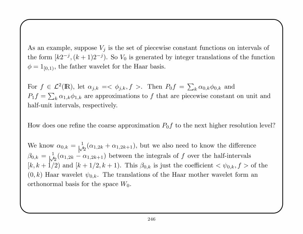
As an example, suppose Vj is the set of piecewise constant functions on intervals of
the form [k2−j, (k + 1)2−j). So V0 is generated by integer translations of the function
φ = 1[0,1), the father wavelet for the Haar basis.
For f ∈ L2(IR), let αj,k =< φj,k, f >. Then P0f =∑
k α0,kφ0,k and
P1f =∑
k α1,kφ1,k are approximations to f that are piecewise constant on unit and
half-unit intervals, respectively.
How does one refine the coarse approximation P0f to the next higher resolution level?
We know α0,k = 1√2(α1,2k + α1,2k+1), but we also need to know the difference
β0,k = 1√2(α1,2k − α1,2k+1) between the integrals of f over the half-intervals
[k, k + 1/2) and [k + 1/2, k + 1). This β0,k is just the coefficient < ψ0,k, f > of the
(0, k) Haar wavelet ψ0,k. The translations of the Haar mother wavelet form an
orthonormal basis for the space W0.
246
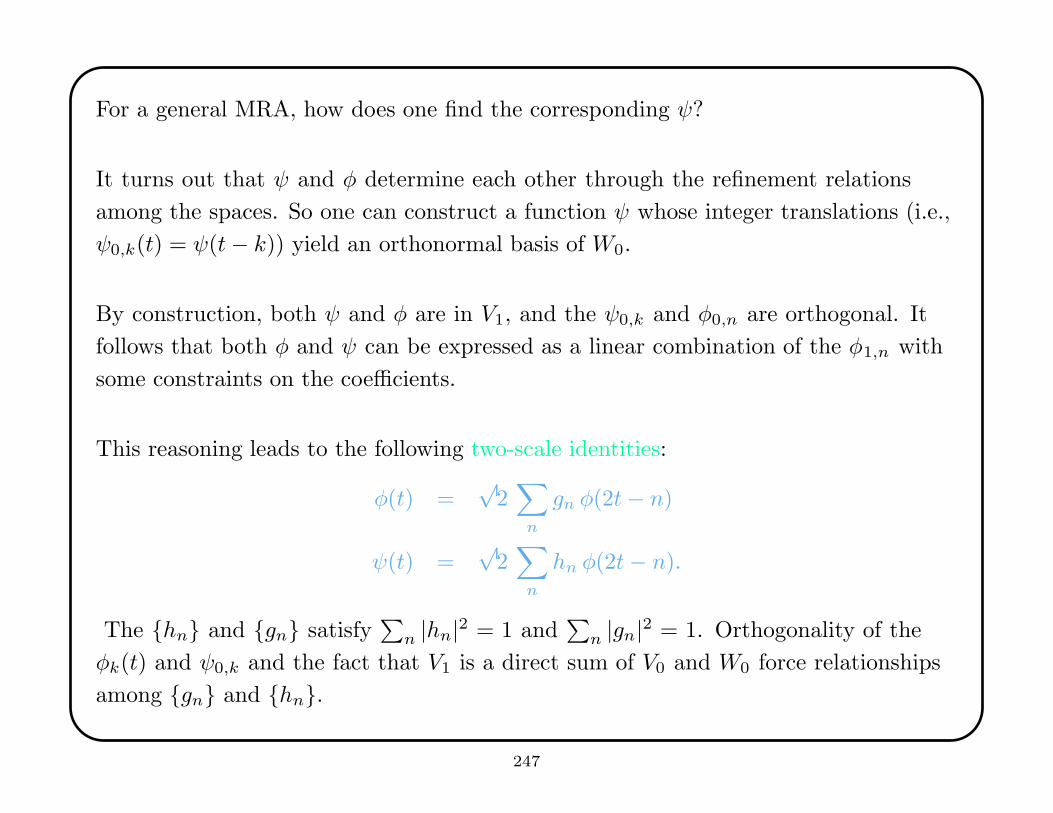
For a general MRA, how does one find the corresponding ψ?
It turns out that ψ and φ determine each other through the refinement relations
among the spaces. So one can construct a function ψ whose integer translations (i.e.,
ψ0,k(t) = ψ(t− k)) yield an orthonormal basis of W0.
By construction, both ψ and φ are in V1, and the ψ0,k and φ0,n are orthogonal. It
follows that both φ and ψ can be expressed as a linear combination of the φ1,n with
some constraints on the coefficients.
This reasoning leads to the following two-scale identities:
φ(t) =√
2∑
n
gn φ(2t− n)
ψ(t) =√
2∑
n
hn φ(2t− n).
The {hn} and {gn} satisfy∑
n |hn|2 = 1 and∑
n |gn|2 = 1. Orthogonality of the
φk(t) and ψ0,k and the fact that V1 is a direct sum of V0 and W0 force relationships
among {gn} and {hn}.
247

For a specific MRA, these relationships provide enough conditions to uniquely identify
mother and father wavelets φ and ψ.
In the Haar case, the sequences are
{gn} = (. . . , 0, 1/√
2, 1/√
2, 0, . . .)
{hn} = (. . . , 0, 1/√
2,−1/√
2, 0, . . .).
In general, it is more convenient to work with the two-scale identities in the Fourier
domain so as to characterize the Fourier transforms φ∗ and ψ∗.
The value of the two-scale identities is in the connections they impose on the wavelet
coefficients. By the two-scale identities,
φjk(t) = 2(j+1)/2∑
n
gnφ(2j+1t− 2k − n)
ψjk(t) = 2(j+1)/2∑
n
hnφ(2j+1t− 2k − n).
248
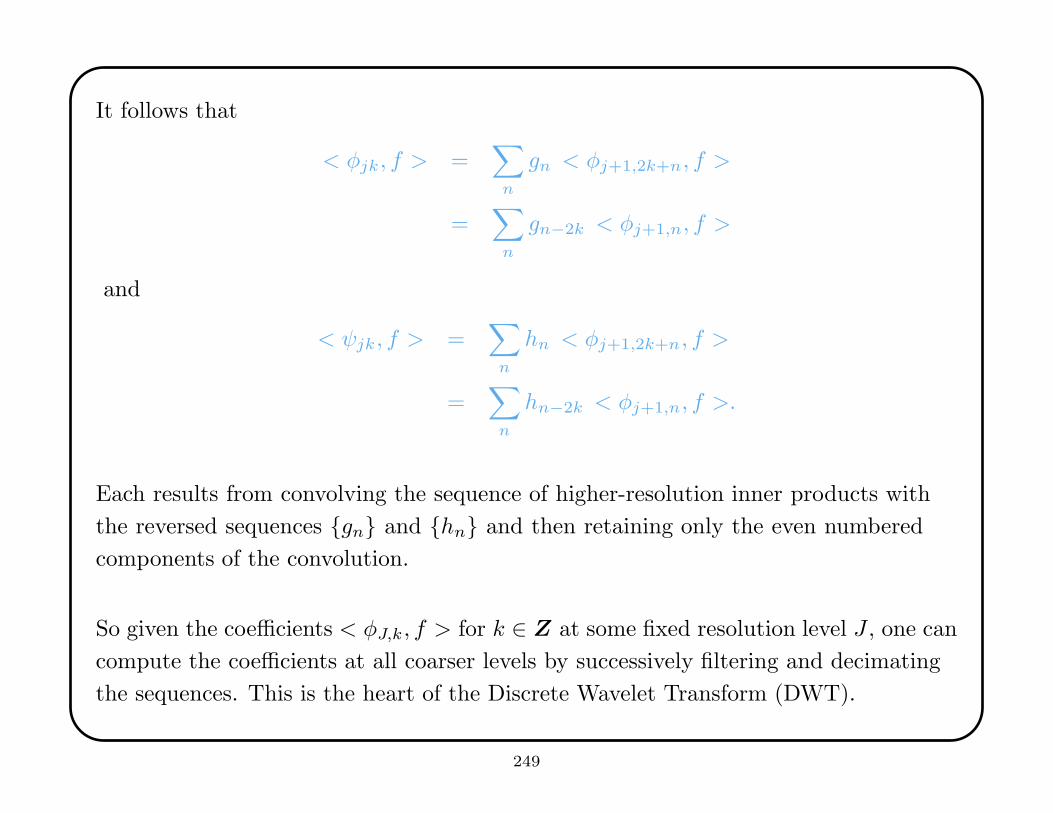
It follows that
< φjk, f > =∑
n
gn < φj+1,2k+n, f >
=∑
n
gn−2k < φj+1,n, f >
and
< ψjk, f > =∑
n
hn < φj+1,2k+n, f >
=∑
n
hn−2k < φj+1,n, f >.
Each results from convolving the sequence of higher-resolution inner products with
the reversed sequences {gn} and {hn} and then retaining only the even numbered
components of the convolution.
So given the coefficients < φJ,k, f > for k ∈ Z at some fixed resolution level J , one can
compute the coefficients at all coarser levels by successively filtering and decimating
the sequences. This is the heart of the Discrete Wavelet Transform (DWT).
249
11. Model Complexity
Our concern is the old bias-variance tradeoff (or overfitting, or capacity control). One
gets the best predictive performance if the family of models strikes the right balance
between the capacity of the family and the accuracy of the performance on the
training set.
Capacity refers to the ability of the model (or machine to perfectly fit the training
sample. If the model is so flexible that it can perform without error on the training
sample, then it is fitting the noise as well as the signal (i.e., overfitting).
A model with too much capacity is like a biologist with perfect memory, who when
shown a dog, cannot identify its species because it has a different number of hairs
than any dog previously studied. A family with too little capacity is like a lazy
biologist who classifies everything with four legs as a dog.
250

11.1 VC Classes
Machine learning theorists have developed clever ways to set bounds on the
performance capability of data mining procedures.
Suppose one has a training sample {(yi,xi)} and wants to predict a future Y value
from measured X values. To do this, one chooses a family of models F = {f(x,θ)}and uses the training sample to find a value of θ that gives “good” performance.
This structure holds in both regression or classification. Here f(·,θ) : IRp → IR, and
the family of functions (the model F) is indexed by θ ∈ Θ.
In multiple linear regression, F consists of all p-dimensional hyperflats and θ are the
regression coefficients. In two-class linear discriminant analysis, F consists of all
p-dimensional hyperflats and the θ are the values in the Mahalanobis-distance rule.
251
The performance of any model in F is assessed through a loss function L[f(x,θ), y].
This measures the deviation between the true value y and a predicted value f(x,θ).
For regression, standard loss functions include:
• absolute loss: L[f(x,θ), y] = |f(x,θ) − y|
• squared error loss: L[f(x,θ), y] = [f(x,θ) − y]2.
For binary classification, labeled so that y ∈ {−1, 1}, a standard loss function is:
• L[f(x,θ], y) = I[−yf(x,θ) > 0].
This last is an indicator function that is 1 iff the sign of y is different from the sign of
f(x,θ). Recall that the usual rule in classification is to predict 1 or -1 according to
the sign of the classification rule f(x,θ).
252
Assume that the joint distribution of future values of (Y,X) is P (y,x). Then the
risk, or expected loss in a future prediction, is
R(θ) =
∫
IRp×IR
L[f(x,θ), y] dP (y,x).
But this cannot be calculated without knowing P (y,x).
Consequently, people use the training sample to calculate the empirical risk:
Re(θ) =1
n
n∑
i=1
L[f(xi,θ), yi].
We want to find a bound on the risk such that with high probability,
R(θ) ≤ Re(θ) +B.
That will tell us how bad our empirical risk is as an estimate of the true risk.
253
In the context of two-class classification, Vapnik (1995, Statistical Learning Theory,
Wiley) showed that with probability q,
R(θ) ≤ Re(θ) +
√
1
n[v + ln(v/h) − ln(q/4)]
where v is a non-negative integer called the Vapnik-Cervonenkis (VC) dimension.
Note that the bound:
• does not depend on the P (y,x);
• assumes that the training sample is a random sample from P (y,x);
• is simple to compute, if v is known;
• can exceed 1, in which case it is useless.
254
The VC dimension depends upon the class F . To start, we consider only the two-class
discrimination problem, so f(x,θ) ∈ {−1, 1}.
A given set of n points can be labeled in 2n possible ways. If for any such labeling,
there is a member of F that can correctly assign those labels, then we say that the set
of points is shattered by F .
The VC dimension for F is defined as the maximum number of points (i.e., training
data) that can be shattered by the elements of F .
Note: If the VC dimension is v, then there exists at least one set of v points that can
be shattered. In general, it is not true that every set of v points can be shattered.
255

intentional blank
256
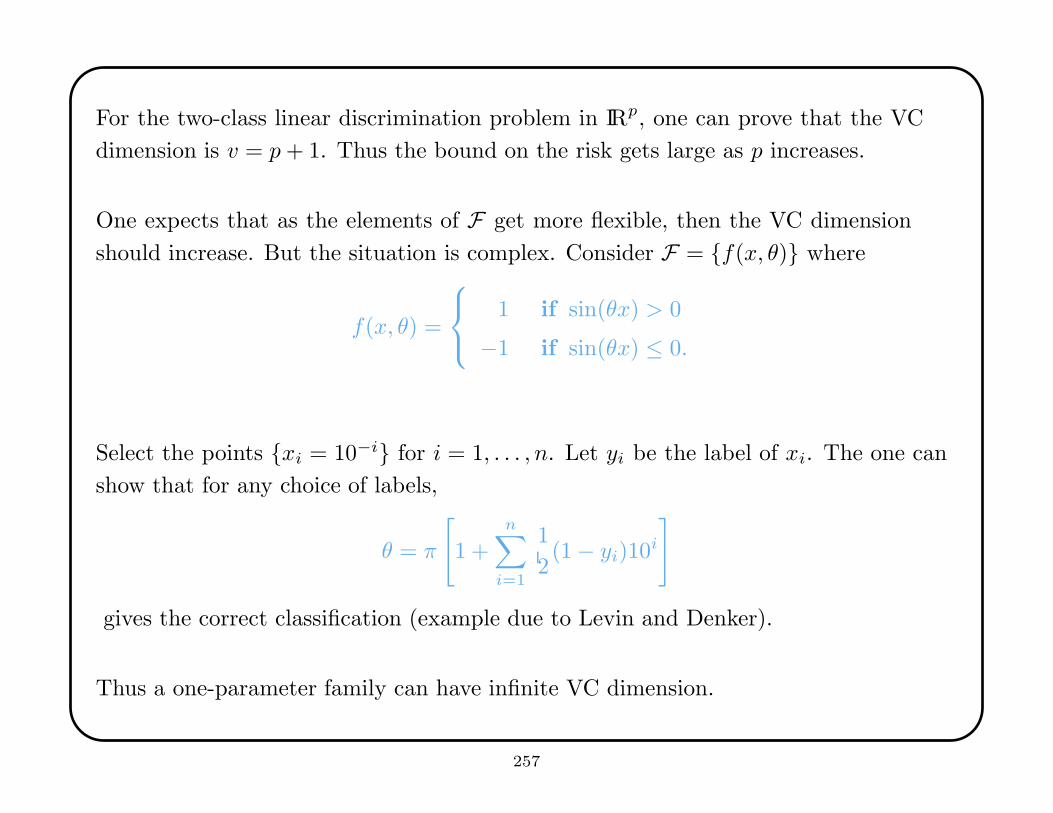
For the two-class linear discrimination problem in IRp, one can prove that the VC
dimension is v = p+ 1. Thus the bound on the risk gets large as p increases.
One expects that as the elements of F get more flexible, then the VC dimension
should increase. But the situation is complex. Consider F = {f(x, θ)} where
f(x, θ) =
1 if sin(θx) > 0
−1 if sin(θx) ≤ 0.
Select the points {xi = 10−i} for i = 1, . . . , n. Let yi be the label of xi. The one can
show that for any choice of labels,
θ = π
[
1 +n∑
i=1
1
2(1 − yi)10i
]
gives the correct classification (example due to Levin and Denker).
Thus a one-parameter family can have infinite VC dimension.
257

intentional blank
258
Consider the 1-nearest neighbor classifier. This F has infinite v, since any number of
arbitrarily labeled points can be shattered. And the empirical risk is zero (unless two
observations with opposite labels coincide). So in this case the VC bound gives no
useful information.
Burges (1998; Data Mining and Knowledge Discovery, 2, 121-167) considers a
“notebook” classifier for a 50/50 mix of population types A and B. The notebook has
m pages; one writes down the labels of the first m training observations, for m < n.
With all subsequent data, predict type A.
The empirical risk (under standard classification loss) for the first m values is 0; the
empirical risk for the next n−m is .5. The true risk on future samples is .5. And the
VC dimension is v = m.
259
The VC-dimension approach to bounding error grew up in the context of support
vector machines. So it is worth noting that for nonlinear machines, the VC dimension
is v = dim(H) + 1, where H is the higher-dimensional space into which the data are
mapped. (Recall section 7.1.3.)
Thus for some kernels, the VC dimension is infinite. To see this in the case the
radial basis function kernel, note that one can shatter a set of points by putting a
small normal distribution on top of each, and labeling it as needed. (This is like the
1-nearest-neighbor classifier.)
Nonetheless, SVMs peform very well. A good choice of kernel enables parsimonious
solutions.
260
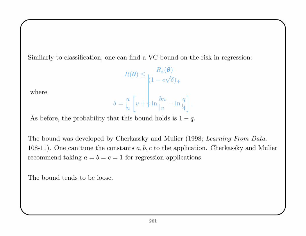
Similarly to classification, one can find a VC-bound on the risk in regression:
R(θ) ≤ Re(θ)
(1 − c√δ)+
where
δ =a
n
[
v + v lnbn
v− ln
q
4
]
.
As before, the probability that this bound holds is 1 − q.
The bound was developed by Cherkassky and Mulier (1998; Learning From Data,
108-11). One can tune the constants a, b, c to the application. Cherkassky and Mulier
recommend taking a = b = c = 1 for regression applications.
The bound tends to be loose.
261
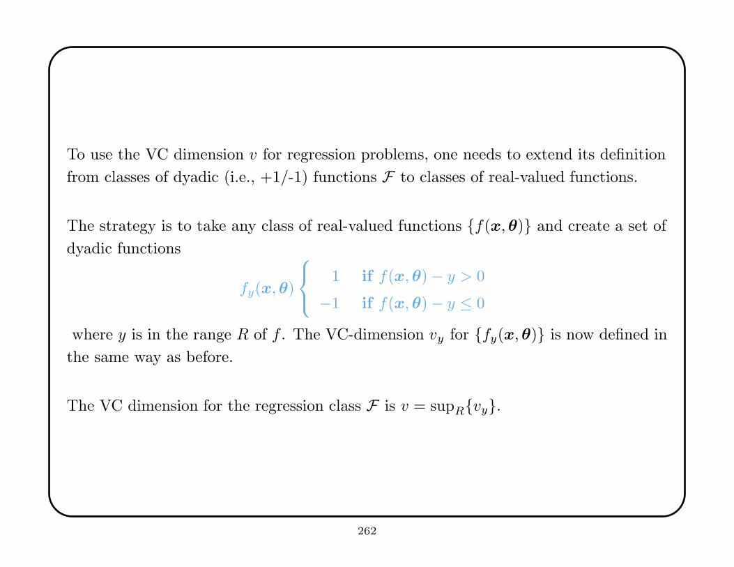
To use the VC dimension v for regression problems, one needs to extend its definition
from classes of dyadic (i.e., +1/-1) functions F to classes of real-valued functions.
The strategy is to take any class of real-valued functions {f(x,θ)} and create a set of
dyadic functions
fy(x,θ)
1 if f(x,θ) − y > 0
−1 if f(x,θ) − y ≤ 0
where y is in the range R of f . The VC-dimension vy for {fy(x,θ)} is now defined in
the same way as before.
The VC dimension for the regression class F is v = supR{vy}.
262
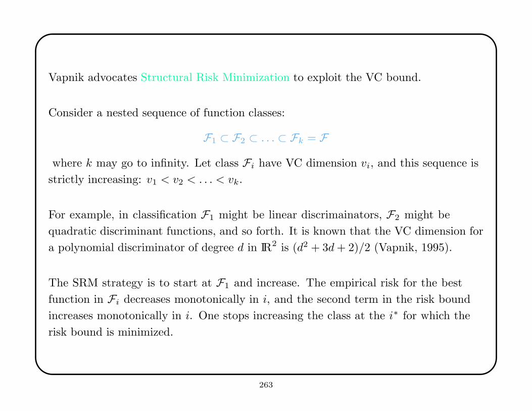
Vapnik advocates Structural Risk Minimization to exploit the VC bound.
Consider a nested sequence of function classes:
F1 ⊂ F2 ⊂ . . . ⊂ Fk = F
where k may go to infinity. Let class Fi have VC dimension vi, and this sequence is
strictly increasing: v1 < v2 < . . . < vk.
For example, in classification F1 might be linear discrimainators, F2 might be
quadratic discriminant functions, and so forth. It is known that the VC dimension for
a polynomial discriminator of degree d in IR2 is (d2 + 3d+ 2)/2 (Vapnik, 1995).
The SRM strategy is to start at F1 and increase. The empirical risk for the best
function in Fi decreases monotonically in i, and the second term in the risk bound
increases monotonically in i. One stops increasing the class at the i∗ for which the
risk bound is minimized.
263
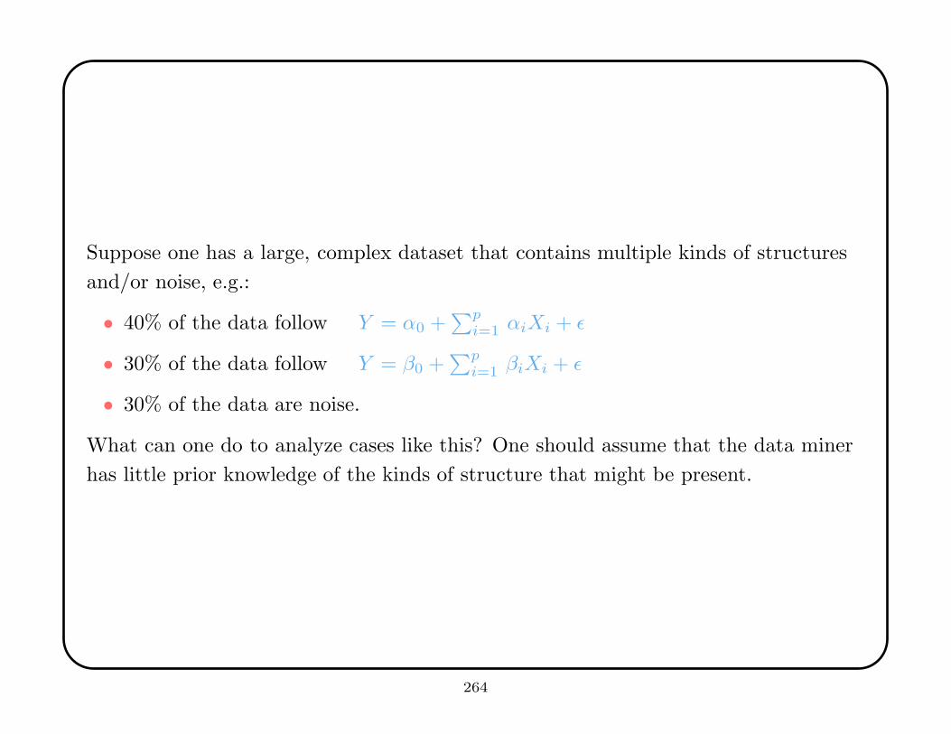
Suppose one has a large, complex dataset that contains multiple kinds of structures
and/or noise, e.g.:
• 40% of the data follow Y = α0 +∑p
i=1 αiXi + ε
• 30% of the data follow Y = β0 +∑p
i=1 βiXi + ε
• 30% of the data are noise.
What can one do to analyze cases like this? One should assume that the data miner
has little prior knowledge of the kinds of structure that might be present.
264
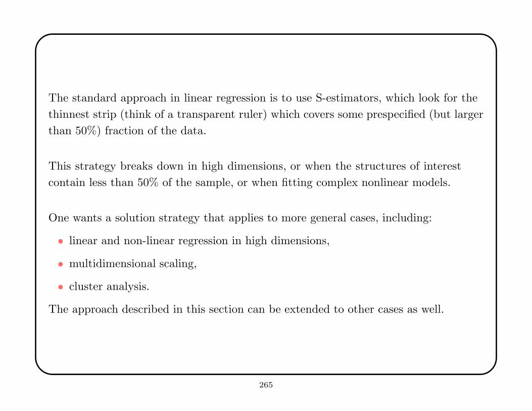
The standard approach in linear regression is to use S-estimators, which look for the
thinnest strip (think of a transparent ruler) which covers some prespecified (but larger
than 50%) fraction of the data.
This strategy breaks down in high dimensions, or when the structures of interest
contain less than 50% of the sample, or when fitting complex nonlinear models.
One wants a solution strategy that applies to more general cases, including:
• linear and non-linear regression in high dimensions,
• multidimensional scaling,
• cluster analysis.
The approach described in this section can be extended to other cases as well.
265
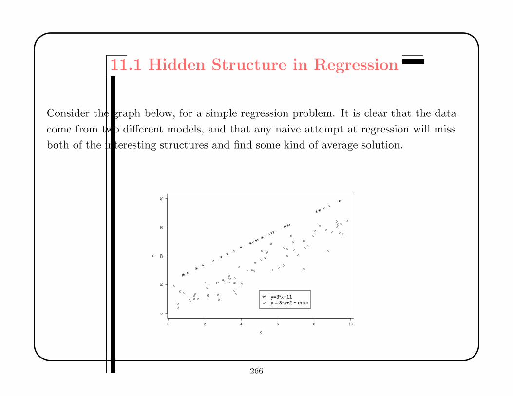
11.1 Hidden Structure in Regression
Consider the graph below, for a simple regression problem. It is clear that the data
come from two different models, and that any naive attempt at regression will miss
both of the interesting structures and find some kind of average solution.
0 2 4 6 8 10
010
2030
40
X
Y
y=3*x+11y = 3*x+2 + error
266
In the linear regression scenario, assume the observations are {Yi,Xi} for i = 1, n and
that Q percent of these follow the model
Yi = β0 + β1Xi1 + . . .+ βpXip + εi where εi ∼ N(0, σ)
where Q, β, and σ are unknown.
One can refer to the Q% of the data as “good” and the rest as “bad”.
Simple Idea:
Start small, with a subsample of only good observations
⇒ add only good observations
⇒ end with a large subsample of good observations.
General procedure:
1. Strategically choose an initial set of d starting subsamples Sj , each of size m
2. Grow the subsamples by adding consistent data
3. Select the largest subsample.
267
The algorithm for choosing the starting subsamples and growing them efficiently is
important in practice.
One starts with a guess about Q, the fraction of good data. In general, this is
unknown, so one might pick a value that is reasonable given
• domain knowledge about the data collection
• scientific interest in a fraction of the data.
From the full dataset {Yi,Xi} one selects, without replacement, d subsamples Sj of
size m.
One needs to choose d and m to ensure that at least one of the starting subsamples
Sj has a very high probability C of consisting entirely of good data (i.e., data that
come from the model).
268
Preset a probability C that determines the chance that the algorithm will work.
The value m, which is the size of the starting-point random subsamples, should be the
smallest possible value that allows one to calculate a goodness-of-fit measure. In the
case of multiple linear regression, that value is p+ 2, and the natural goodness-of-fit
measure is R2.
One solves the following equation for d:
C = IP[ at least one of S1, . . . , Sd is all good ] = 1 − (1 −Qp+2)d.
Example: Q = .8, c = .95, m = 3 (p = 1):
.95 = 1 − [1 − (.8)p+2]d → d = 5
269
Given the d starting-point subsamples Sj , one grows each one of them by adding
observations that do not lower the goodness-of-fit statistic (R2).
Conceptually, for a particular Sj , one could cycle through all of the observations, and
on each cycle augment Sj by adding the observation that provided the largest value of
R2. This cycling would continue until no observation can be added to Sj without
decreasing the R2.
One does this for all of the subsamples Sj . At the end of the process, each augmented
Sj would have size mj and goodness-of-fit R2j . The augmented subsample that
achieves a large value of mj and a large value of R2j is the one that captures the most
important structure in the data.
Then one can remove the data in Sj and iterate to find the next-most important
structure in the dataset.
270
In practice, the conceptual algorithm which adds one observation per cycle is
expensive when the dataset is large or when one is fitting a complex model (e.g.,
doing MARS fits rather than multiple regression). For this reason, one might use a
two-step procedure to add observations.
Fast Search
• Sequentially sweep through all observations not in Si.
• If the observation improves the fitness measure (or perhaps only lowers it by a
small amount η), then
→ add observation to Sj
→ set mj = mj + 1.
If mj < kn then implement slow search.
Slow Search
• Add the observation that improves the FM the most or decreases the fitness
measure the least (regardless of η).
• Repeat until mj = kn.
271
The analyst may pick a value for η that seems appropriately small, and a value for k
that seems appropriately large. These choices determine the runtime of the algorithm
and should reflect practical constraints.
The fast search is greedy, and the order of observations in the cycling matters. The
slow search is less greedy; order does not matter, but it adds myopically. The fast
search can add many observations per cycle through the data, but the slow search
always adds exactly one.
If speed is truly important, then there are other ways to accelerate the algorithm. A
standard strategy would be to increase the number of starting-point subsamples and
combine those that provide similar models and fits as they grow.
The main concern is not to enumerate all
(
n
Qn/100
)
possible subsamples.
272
Some further comments are useful.
1. One does not need to terminate the search at some preset value kn; one can just
grow until the goodness-of-fit measure deteriorates too much.
2. The goodness-of-fit measure should not depend upon the sample size. For R2 this
is easy, since it is just the proportion of variation in Y explained by X. For larger
p, if one is doing stepwise regression to select variables, then one wants to use an
AIC or Mallows’ Cp statistic to adjust the tradeoff in fit between the number of
variables and the sample size.
3. Other measures of fit are appropriate for nonparametric regression, such
as cross-validated within-subsample squared error. But this adds to the
computational burden.
4. One can and should monitor the fit as new observations are added. When one
starts to add bad data, this is quickly visible, and there is a clear “slippery-slope”
effect.
273
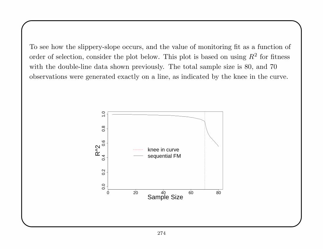
To see how the slippery-slope occurs, and the value of monitoring fit as a function of
order of selection, consider the plot below. This plot is based on using R2 for fitness
with the double-line data shown previously. The total sample size is 80, and 70
observations were generated exactly on a line, as indicated by the knee in the curve.
0 20 40 60 80
0.0
0.2
0.4
0.6
0.8
1.0
Sample Size
R^2 knee in curve
sequential FM
274
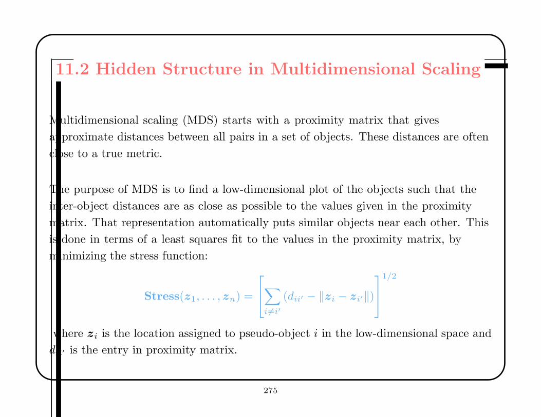
11.2 Hidden Structure in Multidimensional Scaling
Multidimensional scaling (MDS) starts with a proximity matrix that gives
approximate distances between all pairs in a set of objects. These distances are often
close to a true metric.
The purpose of MDS is to find a low-dimensional plot of the objects such that the
inter-object distances are as close as possible to the values given in the proximity
matrix. That representation automatically puts similar objects near each other. This
is done in terms of a least squares fit to the values in the proximity matrix, by
minimizing the stress function:
Stress(z1, . . . , zn) =
∑
i6=i′
(dii′ − ‖zi − zi′‖)
1/2
where zi is the location assigned to pseudo-object i in the low-dimensional space and
dii′ is the entry in proximity matrix.
275
The classic example is to take the entries in the proximity matrix to be the drive-time
between pairs of cities. This is not a perfect metric, since roads curve, but it is
approximately correct. MDS finds a plot in which the relative position of the cities
looks like it would on a map (except the map can be in any orientation; north and
south are not relevant).
MDS seeks is extremely susceptible to bad data. For example, if one had a flight tire
while driving from Rockville to DC, this would create a seemingly large distance. The
MDS algorithm would distort the entire map in an effort to put Rockville far from
DC and still respect other inter-city drive times.
A very small proportion of outliers, or objects that do not fit well in a low-dimensional
representation, can completely wreck the interpretability of an MDS plot. In many
applications, such as text retrieval, this is a serious problem.
276
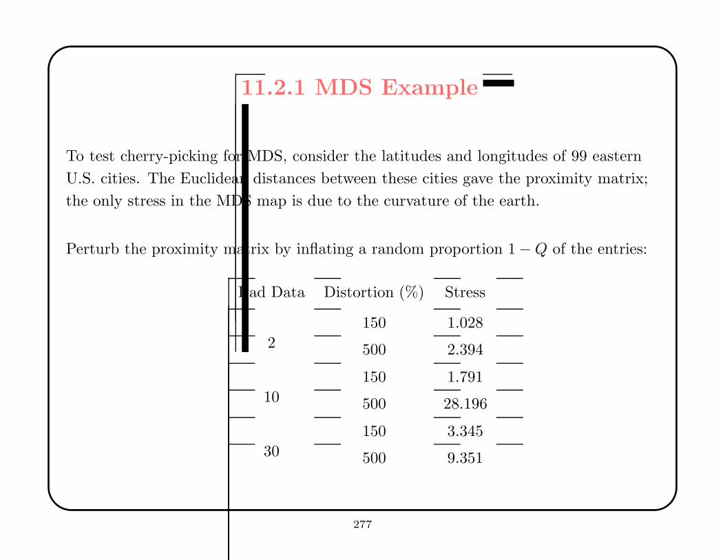
11.2.1 MDS Example
To test cherry-picking for MDS, consider the latitudes and longitudes of 99 eastern
U.S. cities. The Euclidean distances between these cities gave the proximity matrix;
the only stress in the MDS map is due to the curvature of the earth.
Perturb the proximity matrix by inflating a random proportion 1 −Q of the entries:
Bad Data Distortion (%) Stress
150 1.028
2 500 2.394
150 1.791
10 500 28.196
150 3.345
30 500 9.351
277
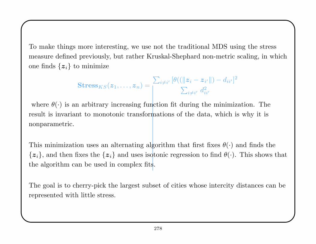
To make things more interesting, we use not the traditional MDS using the stress
measure defined previously, but rather Kruskal-Shephard non-metric scaling, in which
one finds {zi} to minimize
StressKS(z1, . . . , zn) =
∑
i6=i′ [θ((‖zi − zi′‖) − dii′ ]2
∑
i6=i′ d2ii′
where θ(·) is an arbitrary increasing function fit during the minimization. The
result is invariant to monotonic transformations of the data, which is why it is
nonparametric.
This minimization uses an alternating algorithm that first fixes θ(·) and finds the
{zi}, and then fixes the {zi} and uses isotonic regression to find θ(·). This shows that
the algorithm can be used in complex fits.
The goal is to cherry-pick the largest subset of cities whose intercity distances can be
represented with little stress.
278
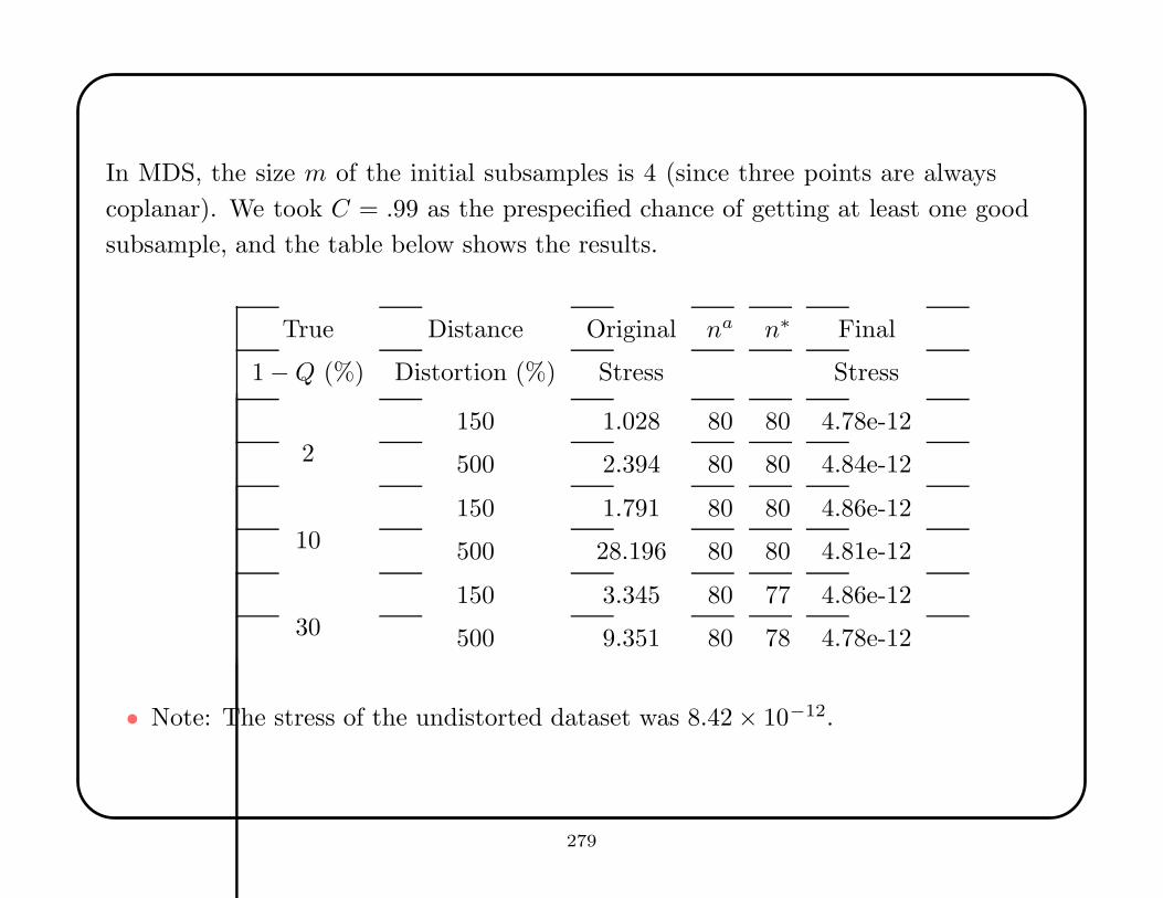
In MDS, the size m of the initial subsamples is 4 (since three points are always
coplanar). We took C = .99 as the prespecified chance of getting at least one good
subsample, and the table below shows the results.
True Distance Original na n∗ Final
1 −Q (%) Distortion (%) Stress Stress
150 1.028 80 80 4.78e-12
2 500 2.394 80 80 4.84e-12
150 1.791 80 80 4.86e-12
10 500 28.196 80 80 4.81e-12
150 3.345 80 77 4.86e-12
30 500 9.351 80 78 4.78e-12
• Note: The stress of the undistorted dataset was 8.42 × 10⁻¹².
279
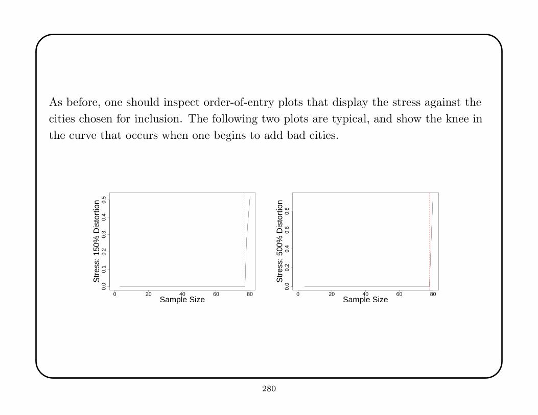
As before, one should inspect order-of-entry plots that display the stress against the
cities chosen for inclusion. The following two plots are typical, and show the knee in
the curve that occurs when one begins to add bad cities.
0 20 40 60 80
0.0
0.1
0.2
0.3
0.4
0.5
Sample Size
Str
ess:
150
% D
isto
rtio
n
0 20 40 60 80
0.0
0.2
0.4
0.6
0.8
Sample Size
Str
ess:
500
% D
isto
rtio
n
280
• This is a simple strategy for identifying primary stucture in complex datasets.
• The calculations are practical in computer-intensive applications, but one needs
to use relatively greedy search algorithms to select observations for inclusion.
• The main computational problem is to scale the algorithm to accommodate very
large samples, but there are obvious ways to address this.
• One can make probabilistic statements about the chance of having a good
starting-point subsample, and this almost leads to a probabilistic guarantee on
the result, but not quite.
• Simulation indicates this works well across a range of problems and situations.
• Once structure is discovered in the data, it can be removed and the process
repeated to find second-order structure.
• The same approach can be used in cluster analysis, where fit is measured by the
ratio of within-cluster variation to between-cluster variation.
281
References
• Breiman, Friedman, Olshen, and Stone, 1984, Classification and Regression Trees,
Wadsworth.
• Green and Silverman, 1994, Nonparametric Regression and Generalized Linear
Models: A Roughness Penalty Approach, Chapman & Hall.
• Hall, 1992, The Bootstrap and Edgeworth Expansion, Springer-Verlag.
• Hastie and Tibshirani, 1990, Generalized Additive Models, Chapman & Hall.
• Hastie, Tibshirani, and Friedman, 2001, The Elements of Statistical Learning,
Springer-Verlag.
• Mitchell, 1997, Machine Learning, McGraw Hill.
• Scott, 1992, Multivariate Density Estimation: Theory, Practice, and
Visualization, Wiley.
• Vapnik, 1996, The Nature of Statistical Learning Theory, Springer-Verlag.
• Vidakovic, 1999, Statistical Modeling by Wavelets, Wiley.
282