introduction to confirmatory analysis · introduction to confirmatory factor analysis multivariate...

Introduction to Confirmatory Factor Analysis

Multivariate Methods in EducationERSH 8350

Lecture #12 – November 16, 2011

ERSH 8350: Lecture 12

Today’s Class

• An Introduction to: Confirmatory Factor Analysis (CFA) Structural Equation Modeling (SEM)

• Placing both within the linear modeling framework The return of the multivariate normal distribution

• A Description of how CFA and EFA differ statistically

• Showing how these methods have subsumed canonical correlation analysis

ERSH 8350: Lecture 12 2

A Brief Review of Exploratory Factor Analysis

• EFA: “Determine nature and number of latent variables that account for observed variation and covariation among set of observed indicators (≈ items or variables)” In other words, what causes these observed responses? Summarize patterns of correlation among indicators Solution is an end (i.e., is of interest) in and of itself

• PCA: “Reduce multiple observed variables into fewer components that summarize their variance” In other words, how can I abbreviate this set of variables? Solution is usually a means to an end


Big Conceptual Difference between PCA and EFA

• In PCA, we get components that are outcomes built from linear combinations of the items: C1 = L11X1 + L12X2 + L13X3 + L14X4 + L15X5 C2 = L21X1 + L22X2 + L23X3 + L24X4 + L25X5 … and so forth – note that C is the OUTCOME

This is not a testable measurement model by itself

• In EFA, we get factors that are thought to be the cause of the observed indicators (here, 5 indicators, 2 factors): X1 = L11F1 + L12F2 + e1 X2 = L21F1 + L22F2 + e1 X3 = L31F1 + L32F2 + e1 … and so forth… but note that F is the PREDICTOR testable


PCA vs. EFA/CFA

Factor

X1 X2 X3 X4

e1 e2 e3 e4

Component

X1 X2 X3 X4

This is not a testable measurement model, because how do we know if we’ve combined items “correctly”?

This IS a testable measurement model, because we are trying to predict the observed covariances between the indicators by creating a factor – the factor IS the reason for the covariance


Big Conceptual Difference between PCA and EFA

• In PCA, the component is just the sum of the parts, and there is no inherent reason why the parts should be correlated (they just are)

But it’s helpful if they are (otherwise, there’s no point in trying to build components to summarize the variables)

“component” = “variable”

The type of construct measured by a component is often called an ‘emergent’ construct – i.e., it emerges from the indicators (“formative”)

Examples: “Lack of Free time”, “SES”, “Support/Resources”

• In EFA, the indicator responses are caused by the factors, and thus should be uncorrelated once controlling for the factor(s)

The type of construct that is measured by a factor is often called a ‘reflective’ construct – i.e., the indicators are a reflection of your status on the latent variable

Examples: Any other hypothetical construct


Intermediate Summary…• PCA and EFA are both exploratory techniques geared loosely

towards examining the structure underneath a series of continuous indicators (items or subscales): PCA: How do indicators linearly combine to produce a set of uncorrelated

linear composite outcomes? EFA: What is the structure of the latent factors that produced the

covariances among the observed indicators (factor = predictor)?

• Involves sequence of sometimes ambiguous decisions: Extraction method Number of factors And then: rotation, interpretation, and factor scores…


Factor Scores in EFA: Just Say No• Factor Indeterminacy (e.g., Grice, 2001):

There is an infinite number of possible factor scores that all have the same mathematical characteristics

Different approaches can yield very different results

• A simple, yet effective solution is simply sum the items that load highly on a factor…“Unit‐weighting” Research has suggested that this ‘simple’ solution is more effective when

applying the results of a factor analysis to different samples – factor loadings don’t replicate all that well

Just make sure to standardize the indicators first if they are on different numerical scales

• Use CFA/SEM – you don’t need the factor scores


CONFIRMATORY FACTOR ANALYSIS


Confirmatory Factor Analysis• Rather than trying to determine the number of factors, and

subsequently, what the factors mean (as in EFA), if you already know (or suspect) the structure of your data, you can use a confirmatory approach

• Confirmatory factor analysis (CFA) is a way to specify which variables load onto which factors

• The loadings of all variables not related to a given factor are then set to zero

• For a reasonable number of parameters, the factor correlation can be estimated directly from the analysis (rotations are not needed)


EFA vs. CFA, continued

• How we get an interpretable solution… EFA: Rotation

All items load on all factors Goal is to pick a rotation that gives closest approximation to simple structure (clear factors, fewest cross‐loadings)

No way of separating ‘content’ from ‘method’ factors CFA: Your job in the first place!

CFA must be theory‐driven You specify number of factors and their inter‐correlations You specify which items load on which factors (yes/no) You specify any unique (error) relations for method variance



• How we judge model fit… EFA: Eye‐balls and Opinion

#Factors? Scree plots, interpretability… Which rotation? Whichever makes most sense… Which indicators load? Cut‐off of .3‐.4ish

CFA: Inferential tests via of Maximum Likelihood Global model fit test Significance of item loadings Significance of error variances (and covariances) Ability to test appropriateness of model constraints or model additions via tests for change in model fit



• What we do with the latent factors… EFA: Don’t compute factor scores…

Factor indeterminacy issues Inconsistency in how factor models are applied to data

– Factor model based on common variance only– Summing items? That’s using total variance (component)

CFA: Let them be part of the model Don’t need factor scores, but they are less indeterminate in CFA than in EFA (although still assumed perfect then)

Better: Test relations with latent factors directly through SEM– Factors can be predictors (exogenous) or outcomes (endogenous) or both at once as needed

– Relationships will be disattenuated for measurement error


CFA Model WITH Factor Means and Item Intercepts

Measurement Model:λ’s = factor loadingse’s = error variancesμ’s = item intercepts

Structural Model:F’s = factor variancesCov = factor covariancesK’s = factor means

F1

X1 X2 X3 X4

e1 e2 e3 e4

λ11 λ21 λ31 λ41

F2

X5 X6 X7 X8

e5 e6 e7 e8

λ52 λ62 λ72 λ82

covF1F2

1μ1

μ2μ3μ4 μ5 μ6

μ7μ8

κ1 κ2

(But some of these values will have to be restricted for the model to be identified)


2 Types of CFA Solutions• CFA output comes in unstandardized and standardized versions:

• Unstandardized predicts scale‐sensitive original item response: Xis = μi + λiFs + eis Useful when comparing solutions across groups or time Note the solution asymmetry: item parameters μi and λi will be given in the item metric, but eis

will be given as the error variance across persons for that item Var(Xi) = [λi2* Var(F)] + Var(ei)

• Standardized solution transformed to Var(Yi)=1, Var(F)=1: Useful when comparing items within a solution (on same scale then) Standardized intercept = μi / SD(Y) not typically reported Standardized factor loading = [λi * SD(F)] / SD(Y) = item correlation with factor Standardized error variance = 1 – standardized λi2 = “variance due to not factor” R2 for item = standardized λi2 = “variance due to the factor”


CFA Model Equations with Item Intercepts

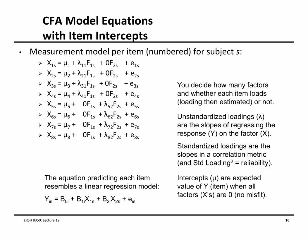
• Measurement model per item (numbered) for subject s: X1s = μ1 + λ11F1s + 0F2s + e1s X2s = μ2 + λ21F1s + 0F2s + e2s X3s = μ3 + λ31F1s + 0F2s + e3s X4s = μ4 + λ41F1s + 0F2s + e4s X5s = μ5 + 0F1s + λ52F2s + e5s X6s = μ6 + 0F1s + λ62F2s + e6s X7s = μ7 + 0F1s + λ72F2s + e7s X8s = μ8 + 0F1s + λ82F2s + e8s

The equation predicting each item resembles a linear regression model:

Yis = Β0i + Β1iX1s + Β2iX2s + eis

You decide how many factors and whether each item loads (loading then estimated) or not.

Unstandardized loadings (λ) are the slopes of regressing the response (Y) on the factor (X).

Standardized loadings are the slopes in a correlation metric (and Std Loading2 = reliability).

Intercepts (μ) are expected value of Y (item) when all factors (X’s) are 0 (no misfit).


Expressing the CFA Model in Matrices: Factor Loadings

• If we put our loadings into a matrix (size p items by m factors)


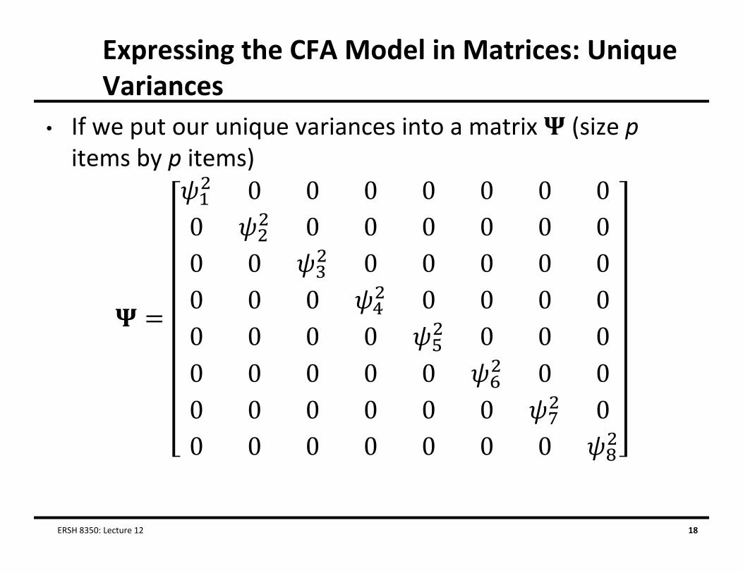
Expressing the CFA Model in Matrices: Unique Variances

• If we put our unique variances into a matrix (size p items by p items)


Expressing the CFA Model in Matrices: Factor Covariances

• If we put our factor covariances into a matrix (size mfactors by m factors):


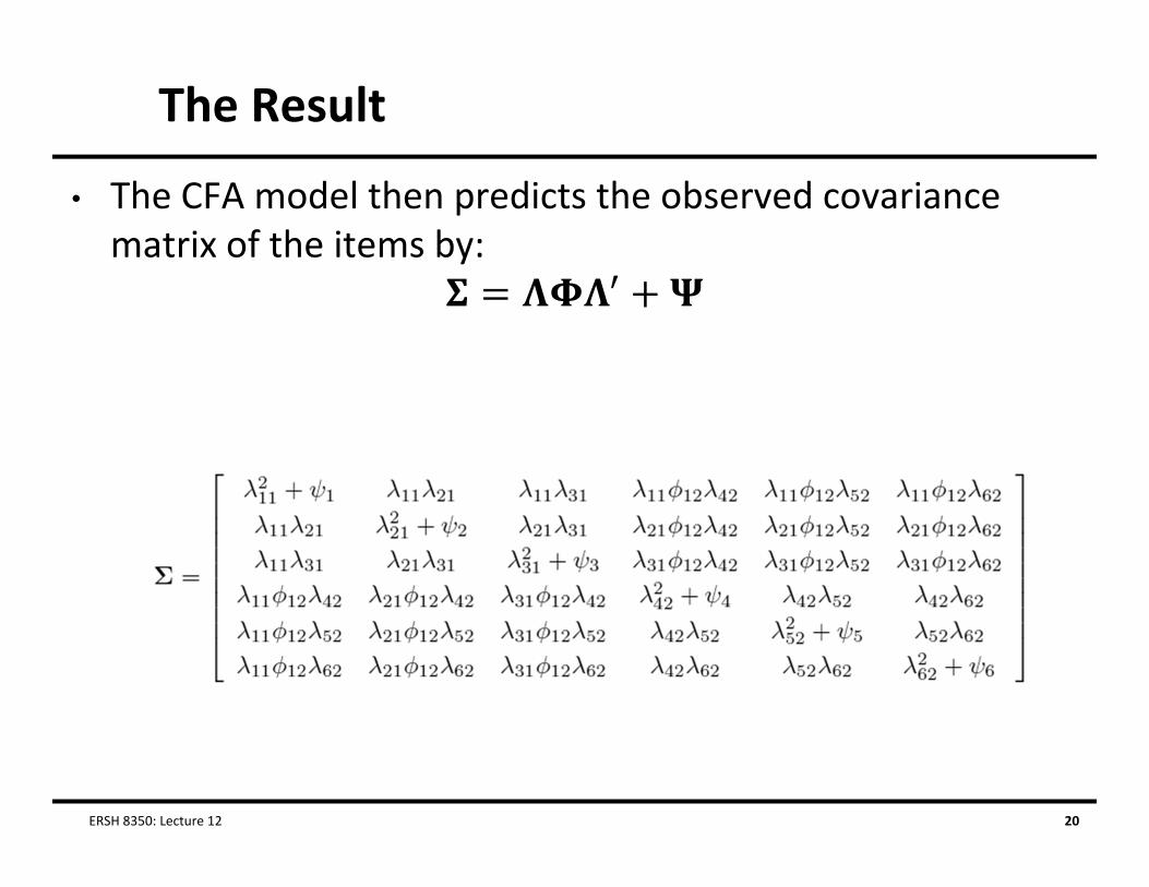
The Result

• The CFA model then predicts the observed covariance matrix of the items by:


CFA Model PredictionsF1 BY X1‐X4, F2 BY X5‐X8

Two items from same factor (room for misfit):• Unstandardized solution: Covariancex1,x4 = λ11*Var(F1)*λ41• Standardized solution: Correlationx1,x4 = λ11*(1)*λ41 std loadings

• ONLY reason for corx1,x4 is common factor (local independence, LI)

Two items from different factors (room for misfit):• Unstandardized solution: Covariancex1,x8 = λ11*covF1,F2*λ82• Standardized solution: Correlationx1,x8 = λ11*corF1,F2*λ82 std loadings

• ONLY reason for corx1,x8 is correlation between factors (again, LI)

Variances are additive (and will be reproduced correctly):• Var(X1) = (λ112)*Var(F1) + Var(e1) note imbalance of λ2 and e


Assumptions of CFA Models• Dimensionality is assumed known (from number of latent traits)

Local Independence e’s are independent after controlling for factor(s)

• Linear model a one‐unit change in latent trait/factor F has same increase in expected item response (Y) at all points of factor (X)

Won’t work well for binary/ordinal data… thus, we need IRT Often of questionable utility for Likert scale data (normality?)

• Goal is to predict covariance between items basis of model fit Variances will always be perfectly reproduced; covariances will not be

• CFA models are usually presented without μi (the item intercept) μi doesn’t really matter in CFA because it doesn’t contribute to the covariance, but

we will keep it for continuity with IRT Item intercepts are also important when dealing with factor mean diffs


CFA Model Identification:Create a Scale for the Latent Variable

• The factor doesn’t exist, so it needs a scale (a mean and variance):

• Two equivalent options to do so

• Create a scale for the VARIANCE: 1) Scale using a marker item

Fix one loading to 1; factor is scaled as reliable part of that marker item

Loading = .9, variance =16? Var(F1) = (.92)*16 = 12.96

2) Fix factor variance to 1 Factor is interpreted as z‐score Can’t be used in other models

with higher‐order factors

F1 = ?

X1 X2 X3 X4

e1 e2 e3 e4

1 λ21 λ31 λ41

F1 = 1

X1 X2 X3 X4

e1 e2 e3 e4

λ11 λ21 λ31 λ41

“Marker Item”

“Z-Score”


CFA Model Identification:Two Options for Scaling the Factor Mean

F1 = 1

X1 X2 X3 X4

e1 e2 e3 e4

λ11 λ21 λ31 λ41

1μ1

μ2 μ3

μ4Κ1 = 0

“Z-Score” Fix factor mean to 0, estimate all item intercepts

Item intercept is expected outcome when factor = 0 (when item = mean)

“Marker Item” Fix 1 item intercept to 0; estimate factor mean

Item intercept is expected outcome when factor = 0 (when item = 0)

F1 = ?

X1 X2 X3 X4

e1 e2 e3 e4

1 λ21 λ31 λ41

10

μ2 μ3

μ4Κ1 = ?


CFA Model Identification:Two Options for Scaling the Factor

• Summary: 2 options for giving the factor a scale: Marker item: Borrow a scale from one of the items

Fix that item’s factor loading to 1 and its intercept to 0 Factor variance is interpreted using the “reliable” part of that item

Z‐score: Put factor on scale of mean=0 and variance=1 Then all item factor loadings and all item intercepts are estimated Can’t be used in higher‐order factor models

• Most common approach is a hybrid: Fix factor mean to 0, estimate all item intercepts “z‐score” Estimate factor variance, fix first item factor loading to 1 “marker”

• In reality, all methods of scaling the factor will fit equivalently well, so long as the marker item loads at all


Factor Model Identification• Goal: Reproduce observed covariance matrix among items with as few estimated

parameters as possible Maximum likelihood usually used to estimate model parameters

Measurement Model: Factor loadings, item intercepts, error variances Structural Model: Factor variances and covariances, factor means

Global model fit is evaluated as difference between model‐predicted matrix and observed matrix (but only the covariances really contribute)

• How many possible parameters can you estimate (total DF)? Total DF depends on # ITEMS p (NOT on # people) Total number of ‘unique elements’ in covariance matrix

Unique elements = each variance, each covariance, each mean Total unique elements = (p(p+1) / 2) + p if 4 items, then ((4*5)/2) + 4 = 14

• Model degrees of freedom (df) Model df = # possible parameters − # estimated parameters


μ2μ1

Under‐Identified Factor: 2 Items

• Model is under‐identified when there are more unknowns then pieces of information with which to estimate them

Cannot be solved because there are an infinite number of different parameter estimates that would result in perfect fit

Example: Solve x + y = 7 ??

F1

X1 X2

e1 e2

λ11 λ21

Total possible df = unique elements = 5

0 factor variances0 factor means2 loadings OR2 item intercepts2 error variances

df = 5 – 6 = -1

If ry1,y2 = .64, then:

λ11 = .800, λ21 = .800 ??λ11 = .900, λ21 = .711 ?? λ11 = .750, λ21 = .853 ??

1 factor variance1 factor mean1 item loading1 item intercept2 error variances

You’d have to set the loadings to be equal for the model to be identified.


Just‐Identified Factor: 3 Items

• Model is just‐identified when there are as many unknowns as pieces of information with which to estimate them

Parameter estimates have a unique solution that will perfectly reproduce the observed matrix

Example: Solve x + y = 7, 3x – y = 1



df = 9 – 9 = 0

Not really a model – more like a description

F1

Y1 Y2 Y3

e1 e2 e3

λ11 λ21 λ31

μ1 μ2 μ3

1 factor variance1 factor mean2 item loadings2 item intercepts3 error variances


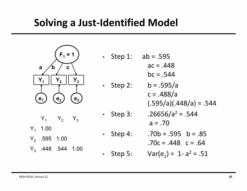
Solving a Just‐Identified Model

• Step 1: ab = .595ac = .448bc = .544

• Step 2: b = .595/ac = .488/a(.595/a)(.448/a) = .544

• Step 3: .26656/a2 = .544a = .70

• Step 4: .70b = .595 b = .85.70c = .448 c = .64

• Step 5: Var(e1) = 1‐ a2 = .51

F1 = 1

Y1 Y2 Y3

e1 e2 e3

a b c

Y1 Y2 Y3

Y1 1.00

Y2 .595 1.00

Y3 .448 .544 1.00


Over‐Identified Factor: 4+ Items

• Model is over‐identified when there are fewer unknowns than pieces of information with which to estimate them

Parameter estimates have a unique solution that will NOT perfectly reproduce the observed matrix

NOW we can test model fit



df = 14 – 12 = 2

Did we do a ‘good enough’ job reproducing the matrix with 2 fewer parameters than was possible to use?

F1

Y1 Y2 Y3 Y4

e1 e2 e3 e4

λ11 λ21 λ31 λ41

1 factor variance1 factor mean3 item loadings3 item intercepts4 error variances

μ1 μ2 μ3 μ4


Indices of Global Model Fit• Primary: obtained model χ2 = FML(N‐1)

Χ2 is evaluated based on model df (# parameters left over) Tests null hypothesis that Σ = S (that model is perfect), so significance is

undesirable (smaller χ2, bigger p‐value is better) Just using χ2 is insufficient, however:

Distribution doesn’t behave like a true χ2 if sample sizes are small or if items are non‐normally distributed

Obtained χ2 depends largely on sample size Is unreasonable null hypothesis (perfect fit??)

• Because of these issues, alternative measures of fit are usually used in conjunction with the χ2 test of model fit Absolute Fit Indices (besides χ2) Parsimony‐Corrected; Comparative (Incremental) Fit Indices


Indices of Global Model Fit• Absolute Fit: χ2

Don’t use ‘ratio rules’ like χ2/df > 2 or χ2/df > 3

• Absolute Fit: SRMR Standardized Root Mean Square Residual Get difference of Σ and S residual matrix Sum the squared residuals in matrix, divide by number of residuals summed Ranges from 0 to 1: smaller is better “.08 or less” good fit

• See also: RMR (Root Mean Square Residual)


Indices of Global Model Fit

Parsimony‐Corrected: RMSEA• Root Mean Square Error of Approximation• Relies on a non‐centrality parameter (NCP)

Indexes how far off your model is χ2 distribution shoved over NCP d = (χ2 – df) / (N‐1) Then, RMSEA = SQRT(d/df) RMSEA ranges from 0 to 1; smaller is better < .05 or .06 = “good”, .05 to .08 = “acceptable”,

.08 to .10 = “mediocre”, and >.10 = “unacceptable” In addition to point estimate, get 90% confidence interval RMSEA penalizes for model complexity – it’s discrepancy in fit per df left in

model (but not sensitive to N, although CI can be) Test of “close fit”: null hypothesis that RMSEA ≤ .05


Indices of Global Model Fit

Comparative (Incremental) Fit Indices• Fit evaluated relative to a ‘null’ model (of 0 covariances)• Relative to that, your model should be great!• CFI: Comparative Fit Index

Also based on idea of NCP (χ2 – df) CFI = 1 – max [(χ2T – dfT),0]

max [(χ2T – dfT), (χ2N – dfN), 0] From 0 to 1: bigger is better, > .90 = “acceptable”, > .95 = “good”

• TLI: Tucker‐Lewis Index (= Non‐Normed Fit Index) TLI = (χ2N/dfN) – (χ2T/dfT)

(χ2N/dfN) – 1 From <0 to >1, bigger is better, >.95 = “good”

T = target modelN = null model


CFA THROUGH AN EXAMPLE


Software for CFA and SEM

• SAS has the CALIS procedure that will estimate the covariance‐portion of a CFA/SEM model Is somewhat dated now

• Instead, I recommend the use of Mplus for CFA and SEM Has many options – fairly easy to use Used in our examples


Our Data: Teacher Ratings

• To demonstrate CFA, we will return to the teacher ratings data we used last week First question: does a one‐factor model fit the data?


One Factor Results


Results Interpretation

• Model parameters: 36 12 item intercepts (means – just ) 12 factor loadings 12 unique variances 0 factor variances (factor variance set to one)

• Model fit: RMSEA: 0.125 (“good” is < 0.05) CFI: 0.867 (“good” > 0.95) TLI: 0.837 (“good” > 0.95)

• Conclusion: One factor model does not fit data very well


Two Factor Model

• What happens when we use some of the information from last week and build a two‐factor model? Competency factor: (13, 14, 15, 16, 17) Friendliness factor: (18, 19, 20, 21)

• But what about items 22, 23, and 24?


Mixing Known Factors with Unknown Items

• Because we more‐or‐less know how 9 of our items work, we can be less specific about the rest of our items Allow them to load onto both factors See if any loadings are significantly different from zero

• There are other methods we could use to see how these items functioned LaGrange multipliers (modification indices)


Two Factor Model #1


Factor Loadings:

• Item 22: No loading onto competency factor

Loading onto friendliness factor

• Items 23 & 24: Loadings about the same magnitude on both factors

Inconclusive results Perhaps we should omit the items?



• Model parameters: 40 12 item intercepts (means – just ) 15 factor loadings 12 unique variances 1 factor covariance 0 factor variances (factor variance set to one)

• Model fit: RMSEA: 0.093 (“good” is < 0.05) CFI: 0.932 (“good” > 0.95) TLI: 0.911 (“good” > 0.95)

• Conclusion: Two factor model does not fit data very well


Perhaps Another Factor?

• Items 23 and 24 seem to have another thing in common: the wording of their questions is very similar Perhaps this indicates another factor


Three Factor Model



• Model parameters: 39 12 item intercepts (means – just ) 12 factor loadings 12 unique variances 3 factor covariances 0 factor variances (factor variance set to one)

• Model fit: RMSEA: 0.082 (“good” is < 0.05) – borderline CFI: 0.947 (“good” > 0.95) – acceptable TLI: 0.931 (“good” > 0.95) – acceptable

• Conclusion: Three factor model fits data adequately


Three Factor Model Estimates


Model Predicted Covariance Matrix

• To show how CFA works…We can confirm in IML the model predicted covariances


SAS…


COMPARING CFA AND EFA


Comparing CFA and EFA

• Although CFA and EFA are very similar, their results can be very different for 2 or more factors

• Recall, EFA typically assumes uncorrelated factors• If we fix our factor correlation to zero, a CFA model becomes very similar to an EFA model But…with one exception…


EFA Model Constraints

• For more than one factor, the EFA model has too many parameters to estimate Uses identification constraints:

where is diagonal

• This constraint puts m*(m‐1)/2 constraints on the loadings and uniquenesses Multivariate constraints


Model Likelihood Function

• Under maximum likelihood estimators, both EFA and CFA use the same likelihood function Multivariate normal Mplus: full information SAS: sufficient statistics (i.e., Wishart distribution for the covariance matrix)


CFA Approaches to EFA

• Therefore, we can approach an EFA model using a CFA We just need to set the right number of constraints for identification

We set the value of factor loadings for a few items on a few of the factors Typically to zero Sometimes to one

We keep the factor covariance matrix as an identity• Benefits:

Our constraints remove rotational indeterminacy of factor loadings

Defines factors with potentially less ambiguity Constraints are easy to see

For some software (SAS), we get more model fit information


EFA with CFA Constraints

• The constraints in CFA are Fixed factor loadings (set to either zero or one)

Use “row echelon” form : One item has only one factor loading estimated One item has only two factor loadings estimated One item has only three factor loadings estimated

Fixed factor covariances Set to zero


Re‐Examining Our EFA of the Teacher Ratings Data – with CFA

• We will fit a series of “just‐identified” CFA models and examine our results

• NOTE: the one factor model CFA model will be identical to the one factor EFA model The loadings and unique variances in the EFA model are the standardized versions from the CFA model


One Factor Results


Two Factor Results


Three Factor Results


Four Factor Results


Model ComparisonModel AIC BIC RMSEA CFI1 Factor 36,747.899 36,823.019 0.125 0.8672 Factor 35,933.855 36,181.232 0.079 0.9583 Factor 35,667.586 35,967.596 0.047 0.9884 Factor 35,593.207 35,940.587 0.025 0.998


Three Factor Model Results


CONCLUDING REMARKS


Wrapping Up

• Today we covered an introduction CFA and SEM• The main point of this lecture is to show how each of these Fits into a mixed modeling framework

Multivariate normal Subsumes the EFA and CCA techniques used in the past

• The link between CFA/SEM and mixed models is important to understand Latent variables = random effects (broadly construed)


Up Next

Date Topic

November 23 No class – Thanksgiving Break

November 30 Structural Equation Modeling/Path ModelingFraming of CFA/SEM in Mixed Models


introduction to confirmatory analysis · introduction to confirmatory factor analysis multivariate...

Documents