introduction to computational physical chemistry · the qualitative model of bonding taught in...

ERICH HUCKEL(1896–1980)

Erich Huckel was born August 9, 1896 in Berlin, Germany and died in 1980. He began uni-

versity studies in physics and mathematics shortly before the outbreak of the First World

War, and was drafted to perform aerodynamics research. He received his doctorate in phys-

ics from the University of Gottingen in 1920 for applications of x-ray diffraction to liquid

crystals, supervised by Peter Debye. After his doctorate, Huckel followed Debye to Zurich,

and it was there that they developed the Debye-Huckel theory of dilute electrolyte solutions.

Following a brief appointment at the Technische Hochschule in Stuttgart, Huckel joined

the faculty of Philips University in Marburg. During a visit to Copenhagen in 1929, Niels

Bohr suggested investigating the carbon-carbon double bond. This led Huckel to develop

the theory of sigma-pi separation in 1930, which he used to explain the restricted rotation

of ethene. Huckel’s brother, Walter—a chemist—suggested applying this to benzene, and in

1931 Huckel generalized his theory to treat conjugated cyclic hydrocarbons, resulting in the

now famous 4n + 2 rule. During the late 1930s he extended this work to pi-conjugated bi-

radicals and unsaturated hydrocarbons. During the Second World War, Huckel was the sole

theoretical physics faculty member at Philips University in Marburg, and was required to

teach all of the courses with any assistants. Overwork and health problems prevented him

from further research work after the war. The importance of Huckel’s pi-electron theory

work was unrecognized for nearly 20 years, which many attribute to poor communication

skills—in particular, his difficult writing style, publishing only in theoretical physics (in-

stead of chemistry) journals, and reluctance to present at conferences.

CHAPTER 6

Huckel Molecular Orbital Theory

The Hartree-Fock calculations discussed in the previous chapter are surprisingly accurate and

relatively easy to perform. Yet neither the underlying conceptual reasons for “why” these an-

swers arise nor the physical interpretation of the results is entirely straightforward. Simplified

model chemistries, such as the Huckel (or “tight-binding”) theory discussed in this chapter,

are one way to make the calculation and its interpretation intelligible. Historically, simplify-

ing the Hamiltonian was a pragmatic way of avoiding numerical calculation before the advent

of computers. Today, these types of simplified electronic structure theories remain useful for

treating the properties of large nanostructures, and as ways of deriving simple explanations

for a variety of chemical phenomena.

6.1 THEORY

Unlike the Hartree-Fock theory discussed in Chapter 5, Huckel theory considers only the pi-

electron wavefunction. This section first reviews the formal sigma-pi separability principle

that enables one to ignore sigma-bonding contributions, and then introduces the simplifying

approximations used to formulate the Huckel model.

6.1.1 Sigma-pi separability

The qualitative model of bonding taught in introductory chemistry courses describes each

atom as having a set of atomic orbitals (AOs) that combine to form molecular orbitals (MOs).

As discussed in our treatment of the variational principle (Section 4.4.2), this is just a state-

ment that the basis functions (AOs) form linear combinations (MOs) that are variational

eigenstates of the molecular Hamiltonian. One also learns that planar molecules with dou-

ble bonds, such as ethylene, C2H2, or benzene, C6H6, combine these AO functions to form

σ and π MOs. Symmetry considerations separate these two different types of MOs. Suppose

that the molecule is oriented in the xy-plane. The σ bonds are symmetrical (even symmetry)

with respect to this plane, and thus can only be comprised of AOs having the same symme-

try. In this case, these are s-like AOs and the 2px- and 2py-like AOs that are in the plane of

the molecule. In contrast the π bond changes sign (odd symmetry) across the plane of the

molecule, and thus can only be comprised of AOs with that symmetry, i.e., a 2pz AO whose

nodal plane coincides with the plane containing the molecule. The separability of the σ and

139

140 6. Huckel Molecular Orbital Theory

π MOs arises from this symmetry difference.1 Therefore, the electronic structure for each

of these sets of MOs can be found independently of each other. The σ -bonding electronic

structure is less interesting, since σ MOs are spatially localized and tend to be less reactive. In

contrast, the π MOs tend to be spatially delocalized over the molecule (and hence can vary

greatly between different types of molecules), and are generally more reactive. The transitions

between occupied and unoccupied π molecular orbitals also give rise to ultraviolet and visi-

ble (UV/vis) spectroscopic features,2 in contrast to the transitions between σ orbitals, which

are much higher in energy for organic molecules. For these reasons, focusing completely on

the π-electron part of the molecular Hamiltonian will shed light on many of the properties,

spectroscopy, and reactivity of this class of molecules.

6.1.2 Simplifying assumptions

Conceptually, the π-electron MO, ψ , is a superposition of 2pz (AO) basis functions, φn, cen-

tered on each atom, n. In principle, one could define this basis in terms of Slater- or Gaussian-

type functions, and then compute the overlap, one-electron Hamiltonian, Coulomb, ex-

change, and Fock matrices needed for the Hartree-Fock equations discussed in Chapter 5.

Such a first-principles or ab initio approach becomes computationally expensive for large

molecules, due to the large number of integrals required. Instead, Huckel theory proposes

a simple model for constructing these matrices, based on three assumptions.

Assumption 1: Basis function orthonormality

The first assumption is that the basis functions are orthonormal, i.e, Snm = ∫φ∗

nφm d3�r =

δnm. Although it is straightforward to construct normalized functions, atomic orbitals cen-

tered on different nuclei are typically not orthogonal (as in previous experiences with the 1s

atomic orbitals of the hydrogen molecule in Section 5.2). Numerical calculations show that

the overlap between adjacent carbon 2pz AOs (i.e., nearest-neighbor atoms “bonded” to each

other) in a typical molecule are on the order of 0.1, and this rapidly goes to zero for more

distant atoms. This relatively small contribution suggests that they can be approximately set

to zero as an assumption in the model. The practical benefit of this assumption is that it elim-

inates the need to compute the overlap matrix elements, and also reduces the problem to a

simple (rather than generalized) eigenvalue problem.

Assumption 2: Ignore the two-electron contributions

The second assumption is that an “effective” one-electron problem—that does not depend on

the charge density matrix—can be used instead of the full many-electron Hamiltonian. This

assumption may be rationalized in two ways: (i) only the one-electron terms in Eq. (5.46)

are necessary because the Coulomb and exchange integral terms are comparatively small; or

(ii) the effective one-electron problem is actually just the (mean field) Fock matrix, whose

1. This separability is only strictly true for planar molecules. In nonplanar molecules, there is a (relatively)small mixing between π and σ MOs that is often ignored.2. i.e., pretty colors

6.1 theory 141

matrix elements may be chosen to contain an average Coulomb and exchange contribution

(but without explicitly calculating these). The practical benefit of this assumption is that it

obviates both the Coulomb and exchange matrix elements integral calculations, as well as the

iterative self-consistent calculation. Two potential negative consequences of this assumption

are that (i) the effects of charge redistribution in the molecule no longer appear in the model

Hamiltonian, since the charge density matrix does not modify the one-electron effective

Hamiltonian; and (ii) there is no difference between the energies of singlet and triplet (or

other) spin configurations having the same orbital occupation, due to the lack of exchange

terms.

Assumption 3: One-electron Hamiltonian terms are parameterized to bond types

The third assumption is that these one-electron Hamiltonian terms, Hnm = ∫φ∗

nHφm d3�r ,

are accurately described by empirical values, obtained by fitting to reproduce experimental

spectroscopic or thermodynamic data. In principle, the experimental properties “know” the

values of these integrals, so one can rationalize this as a circuitous way of having Nature “com-

pute” these values. The fitting procedure assumes that Hnm is only nonzero when n and m are

either the same (i.e., an AO interacting with itself) or adjacent to each other (n and m are

nearest neighbors connected by a “bond” in a Lewis diagram). This is plausible because the

Hamiltonian matrix elements scale roughly as the overlap between AOs, and therefore fall

off very quickly beyond nearest neighbors.3 In practice, this assumption eliminates the need

to perform any integration; the Hamiltonian matrix elements are determined solely by the

connectivity of the atoms. This assumption has the potential negative consequence that the

results no longer derive from the first principles of the Schrodinger (or Hartree-Fock) equa-

tions, but are instead dependent on parameterization to a limited set of (potentially faulty)

experimental data. It would be useless if every molecule needed a unique set of parameters, so

a further implicit assumption is that these matrix elements depend only on the types of atoms

that are connected, independent of details about their molecular environment, such as local

variations in charge or bond length. In other words, the Huckel Hamiltonian matrix element

describing the interaction between two adjacent carbon atoms is assumed to be the same, re-

gardless of whether those two carbon atoms are in an ethylene molecule or in a naphthalene

molecule.

Summary

To summarize:

. the overlap matrix is now simply the identity matrix

. the Hamiltonian matrix is now solely defined by atom connectivity, without depen-

dence on charge redistribution within the molecule or the precise inter atomic geometry

3. The astute reader will note an inconsistency in arguing that the nearest-neighbor Hamiltonian matrixelements are nonzero because the AO overlaps of those atoms are nonzero, while the first assumption tookthe AOs as orthonormal. Apparently, this did not bother Huckel.


Despite this radical oversimplification of the problem, Huckel theory explains many of the

properties of planar aromatic molecules, as discussed in this chapter. We will first perform

a few classic small molecule problems to demonstrate how to perform elementary Huckel

calculations. This is followed by a discussion of some useful advanced features in Mathematica

that will help construct more complicated Huckel calculations and plot your results. Finally,

we will discuss and demonstrate how to calculate various chemical properties and reactivity

trends using Huckel theory.

6.2 ELEMENTARY EXAMPLES

Three canonical examples are typically used to illustrate Huckel theory calculations. First, the

simplest possible π-electron system is the ethylene molecule. Second, the generalization to

larger linear molecules is demonstrated using the butadiene molecule. Third, the generaliza-

tion to cyclic molecules is demonstrated using the benzene molecule.

6.2.1 Ethylene

The simplest example of Huckel molecular orbital theory is the ethylene molecule:

Here the carbons participating in the π-electron system are arbitrarily labeled 1 and 2. Huckel

theory treats only the π-electron Hamiltonian, and thus only the 2pz AOs are used as the ba-

sis. Each row/column in the Hamiltonian matrix corresponds to the matrix element involving

the 2pz AO located on a specific carbon atom.

H =[

H11 H12

H21 H22

](6.1)

Since each carbon atom has only one 2pz AO, the “which atom” index is identical to a

“which AO” (i.e., “which basis function”) index. We’ll construct the Hamiltonian matrix in

this basis, following the approximations discussed above. Because all the atoms are the same,

it is convenient to choose Hrr = 0, i.e., the Hamiltonian matrix element of a carbon 2pz

atomic orbital with itself. This choice makes all the diagonal terms equal to zero. Physically,

this is equivalent to defining the energy of an isolated carbon 2pz AO as the “zero” of energy;

energies that are lower or higher than this zero correspond to net bonding or antibonding

relative to the isolated atoms. Because the two carbon atoms are “bonded” to each other, they

have a nonzero off-diagonal matrix element, Hrs = t = 〈r|H |s〉.

H =[

0 t

t 0

](6.2)

It is easiest to define the connectivity using just ones and zeros,

MatrixForm[ hMatr={{0,1},{1,0}} ] (* ethylene Hamiltonian *)

6.2 elementary examples 143

and then multiply the entire matrix by the desired value of t before computing the eigen-

values and eigenvectors. A typical value, based on reproducing spectroscopic transitions of

small polyaromatic molecules, is t = −2.7 eV. The particular numerical value depends on the

spectroscopic or thermodynamic parameterization. Although this changes the quantitative

eigenvalues, both the eigenvectors and the qualitative ordering of the eigenvalues are inde-

pendent of the precise value. One way to avoid making an explicit choice for this value is to

use t as a unit of energy when describing Huckel theory results for polyaromatic hydrocar-

bons. (Note that t must be negative in order for the “bonding” MO to be lower in energy than

the “antibonding” MO.)

Having constructed the Hamiltonian matrix, hMatr, its eigenvalues (evals) and eigen-

vectors (evecs) are obtained as in previous chapters.

t=-2.7; (* typical π-π Hamiltonian matrix element, in eV *)

{evals,evecs}=Eigensystem[t*hMatr] (* get eigenvalues/vectors *)

{{-2.7 2.7}, {{-0.707107, -0.707107}, {-0.707107, 0.707107}}}

The π MOs are comprised of an equal superposition of the two AO basis functions. The

set of eigenvectors, evecs, contains the linear variational coefficients for each state.

evecs

{{-0.707107, -0.707107}, {-0.707107, 0.707107}}

Note how the low-energy solution (first eigenvector) has both AOs with the same phase

(both terms in the eigenvector have the same sign), and the high-energy solution (second

eigenvector) has a node between the atoms (the terms have opposite signs, so they must cross

through zero). This corresponds to the bonding and antibonding π molecular orbitals that

you learned about during introductory chemistry.

The molecular orbitals should be orthonormal. Consequently, the vector representation of

the molecular orbitals stored in the evecs vector must be orthonormal. Since Huckel theory

assumes the overlap matrix is an identity matrix, evaluating 〈ψ |ψ〉 is equivalent to taking the

vector scalar product (“dot product”) of the two vectors (as was introduced in Section 4.3.2).

Let’s test the normalization of the two eigenstates:

evecs[[1]].evecs[[1]] (* check normalization for first MO... *)

evecs[[2]].evecs[[2]] (* ...and second MO *)

1.

1.

Testing the orthogonality of the two states is left as an exercise for the reader.

Transitions between energy levels occur when the molecule absorbs a photon. Transitions

between electronic states are typically in the UV/vis spectrum for π-conjugated molecules.

The lowest-energy electronic transition, and thus the lowest-energy photon the molecule

can absorb in this spectral region, occurs between the highest-occupied molecular orbital

(HOMO) and the lowest-unoccupied molecular orbital (LUMO). The energy difference be-

tween these is referred to as the HOMO-LUMO gap. Because Huckel theory considers only


the π electrons, each carbon atom contributes one π electron. In the current case of ethylene,

the molecule has two π electrons, and hence one doubly occupied molecular orbital. Thus,

ethylene’s HOMO-LUMO gap is the difference between the second (lowest-unoccupied) and

first (highest-occupied) molecular orbital energy, stored in the list of eigenvalues, evals:

evals[[2]]-evals[[1]] (* in eV, since t is defined in eV units *)

5.4

Since the value of t, defined earlier in the calculation, is in electron volts (eV), the HOMO-

LUMO gap will also be in electron volts.

6.2.2 Butadiene

The next example is the butadiene molecule:

Once again, the diagram includes (arbitrarily ordered) index labels for each carbon atom in

the π-electron system. In this basis, the Hamiltonian matrix has the form

H =

⎡⎢⎢⎢⎢⎣

H11 H12 H13 H14

H21 H22 H23 H24

H31 H32 H33 H34

H41 H42 H43 H44

⎤⎥⎥⎥⎥⎦ . (6.3)

Following the simplifying assumptions described in Section 6.1.2, Huckel theory assumes

that the off-diagonal matrix elements are nonzero only when the two 2pz atomic orbital

basis functions are adjacent to each other. Thus, H12 = t , but H13 = H14 = 0, using the

atomic labeling scheme above. As before, the diagonal matrix elements, Hrr = 0, defines

unbonded carbon atoms as the system’s zero of energy. These simplifying assumptions result

in a Hamiltonian matrix element of the form

H =

⎡⎢⎢⎢⎢⎣

0 t 0 0

t 0 t 0

0 t 0 t

0 0 t 0

⎤⎥⎥⎥⎥⎦ . (6.4)

Observe that the Hamiltonian matrix is Hermitian (Hrs = H ∗sr

)—or more strictly speak-

ing, real symmetric, since t is real valued (t = t∗). This is true regardless of the labeling scheme

used to index the 2pz AO basis functions in the molecule. Moreover, so long as the connec-

tivity is the same, any consistent labeling scheme will give equivalent eigensolutions.

To implement this in Mathematica, we first construct the connectivity matrix and then

multiply by t to scale the energies to experimental units:


t=-2.7;

MatrixForm[ hMatr={{0,1,0,0},{1,0,1,0},{0,1,0,1},{0,0,1,0}} ]

{evals,evecs}=Eigensystem[t*hMatr]

{{4.36869, -4.36869, 1.66869, -1.66869},

{{-0.371748, 0.601501, -0.601501, 0.371748}, {0.371748, 0.601501,

0.601501, 0.371748}, {0.601501, -0.371748, -0.371748, 0.601501},

{0.601501, 0.371748, -0.371748, -0.601501}}}

According to the Aufbau principle, the MO occupations are determined by filling in the

electrons from lowest energy to highest energy. However, Mathematica returns numerical

eigenvalues sorted by magnitude, rather than by value. Simply applying Sort[] would only

sort the eigenvalues, without also shuffling the eigenvectors in the corresponding order. To

sort the corresponding list of eigenvectors, the Ordering[] function can be used to generate

a list that will correctly shuffle the eigenvalues into lowest-to-highest numerical order. This

shuffling list can be applied to both evals (the list of eigenvalues) and evecs (the list of

eigenvectors) to sort them in the same order. More specifically:

sortEigen=Ordering[evals]; (* find ascending sorting pattern *)

evals=evals[[sortEigen]] (* sort eigenvalues *)

evecs=evecs[[sortEigen]] (* sort eigenvectors *)

{-4.36869, -1.66869, 1.66869, 4.36869},

{{0.371748, 0.601501, 0.601501, 0.371748},

{0.601501, 0.371748, -0.371748, -0.601501},

{0.601501, -0.371748, -0.371748, 0.601501},

{-0.371748, 0.601501, -0.601501, 0.371748}}

To simplify the subsequent calculations, let us define a function, sortedEigensystem[],

that returns sorted eigenvalues and eigensystems of an input hamiltonian:

sortedEigensystem[hamiltonian_]:=Module[{evals,evecs,sortEigen},

{evals,evecs}=Eigensystem[hamiltonian];

sortEigen=Ordering[evals]; (* find ascending sorting pattern *)

evals=evals[[sortEigen]]; (* sort eigenvalues *)

evecs=evecs[[sortEigen]]; (* sort eigenvectors *)

{evals,evecs} (* return list of sorted eigenvalues and eigenvectors *)

]

To confirm that it implemented correctly, let’s reproduce the last calculation:

{evals,evecs}=sortedEigensystem[t*hMatr]

{{-4.36869, -1.66869, 1.66869, 4.36869},

{{0.371748, 0.601501, 0.601501, 0.371748}, {0.601501, 0.371748,

-0.371748, -0.601501}, {0.601501, -0.371748, -0.371748, 0.601501},

{-0.371748, 0.601501, -0.601501, 0.371748}}}


What is the significance of this result? The lowest-energy eigenstate of butadiene has no

nodes in the molecular orbital (MO) wavefunction (observe how all the eigenvector coeffi-

cients in evecs[[1]] are positive), and successively higher-energy states have an increasing

number of nodes between the atoms. This is the same type of nodal structure observed in

the 1D-PIB wavefunctions. In fact, the free-electron model of polyenes treats the conjugated

π system as a 1D-PIB problem. This correspondence is unsurprising given the mathemat-

ical similarity of the Hamiltonian matrix here to the 1D finite difference Hamiltonian for

the 1D PIB in Chapter 2. In the finite difference calculation, box-shaped basis functions

were used to describe the eigenvectors and Hamiltonian. Here the basis of the eigenvectors—

and the basis used to construct the Hamiltonian—are the different atom-centered AO basis

functions. Despite the different basis functions, the Hamiltonian matrices in both cases are

tri-diagonal—they have nonzero entries only on the main diagonal and the first diagonals

above and below the main diagonal—and hence the eigenvectors have similar nodal patterns.

Finally, the HOMO-LUMO gap of this 4-π-electron-containing molecule can be calcu-

lated by taking the difference between the highest-occupied and lowest-unoccupied molecu-

lar orbital energies:

evals[[3]]-evals[[2]] (* HOMO-LUMO gap, in eV *)

3.33738

This is smaller than the ethylene HOMO-LUMO gap, consistent with the predictions of the

1D-PIB free-electron model for conjugated π systems.

6.2.3 Benzene

A third classic example of Huckel theory is the benzene molecule:

Each carbon atom is connected to two nearest neighbors (i.e., “left” and “right”), forming

a ring of atoms. Labeling each atom 1, 2, 3, 4, 5, 6 (with each of these corresponding to a

particular row or column index in the Hamiltonian matrix), the connection between atoms

1 and 6 closes the ring. Rather than constructing hMatr as a list of lists, it is simpler to input

this using the graphical editor, accessed by the Insert >Table >Matrix >New . . . menu. As

in the previous examples, the eigenvalues and eigenvectors (molecular orbitals, MOs) of the

Hamiltonian are obtained by solving the matrix eigenvalue problem numerically:4

4. Do not be alarmed if your eigenvectors differ by a minus sign from the ones shown here. Here all ofthe orbital coefficients for the lowest-energy molecular orbital have a negative sign, but in some previousversions of Mathematica these are all positive. Physically and mathematically, the difference in sign is just


{{-5.4, -2.7, -2.7, 2.7, 2.7, 5.4},{{-0.408248, -0.408248, -0.408248, -0.408248, -0.408248, -0.408248},

{0.288675, -0.288675, -0.57735, -0.288675, 0.288675, 0.57735},

{0.5, 0.5, -1.64477 × 10−16, -0.5, -0.5, 0.},

{-0.5, 0.5, 1.64477 × 10−16, -0.5, 0.5, 0.},

{0.288675, 0.288675, -0.57735, 0.288675, 0.288675, -0.57735},

{0.408248, -0.408248, 0.408248, -0.408248, 0.408248, -0.408248}}}

Benzene has six π electrons (one from each carbon 2pz AO), so the first three molecular or-

bitals are doubly occupied. The list of eigenvalues, evals, indicates that the highest-occupied

MO (evals[[3]]) and lowest-unoccupied MO (evals[[4]]) are both doubly degenerate

(with the evals[[2]] and evals[[5]] levels, respectively).

As in Section 6.2.1, we can check the orthonormalization of the states by taking the dot

product of each eigenvector with itself. First, we can test the normalization of the first few

molecular orbitals,

evecs[[1]].evecs[[1]] (* check normalization *)

evecs[[2]].evecs[[2]]


1.

1.

1.

to confirm that the states are properly normalized to one. (Testing the other states is left as an

exercise for the reader.) Second, we test the orthogonality of a few of the pairs of states:5

evecs[[1]].evecs[[2]] (* check orthogonality *)


3.88578 × 10−16

-2.77556 × 10−17

The result is not precisely zero, but instead is a very small number, due to the finite numer-

ical precision of the eigenvectors. (Indeed, you may get a slightly different small number,

an irrelevant global phase; only changes between positive and negative signs within a particular molecularorbital are important.5. In some older versions of Mathematica, degenerate eigenvectors were not always orthogonal to eachother, conflicting with this requirement. However, since any linear combination of degenerate MOs is itselfa valid eigensolution, these can be combined to generate a set of orthogonal solutions, by applying theOrthogonalize[] function to the set of eigenvectors.


depending on the default settings for the eigenvalue solver in your particular version of Math-

ematica.) For our scientific purposes, these very tiny values are effectively zero. If you wish to

have a simpler output, the Chop[] function can be used to replace real numbers such as these

that are very close to zero by the exact integer value of zero. However, in this case it is a purely

aesthetic decision, and will have no impact on subsequent calculations.

6.3 ADVANCED MATHEMATICA TECHNIQUES

The strategy demonstrated in the previous section—drawing a molecule, numbering the

atoms, constructing the corresponding Hamiltonian matrix, and finding the Eigen-

values[] and Eigenvectors[]—corresponds to the traditional approach for solving

Huckel theory problems. This section investigates ways of using Mathematica to stream-

line the calculations and visualize results. First, we’ll demonstrate the use of Mathematica’s

ChemicalData[] functionality to query an online chemical structure database and use the

results to construct the Hamiltonian matrix. Then, we’ll see how to create Graphics[]

comprised of basic shapes.

6.3.1 Using ChemicalData[]

The built-in ChemicalData[] function provides access to a number of chemical properties.

Among these are the atom connectivities, which can be used to automate construction of the

Huckel Hamiltonian matrix, and the atom positions, which can be used to plot the results.

ChemicalData[] takes two arguments, provided as strings: (1) the name of the molecule

and (2) the desired property to return. The property StructureDiagram returns a standard

two-dimensional organic-chemistry skeletal-formula diagram, excluding hydrogen atoms:

struct2d=ChemicalData["Benzene","StructureDiagram"]

The property MoleculePlot is a 3D diagram that can be rotated interactively (try it!):

struct3d=ChemicalData["Benzene","MoleculePlot"]

6.3 advanced mathematica techniques 149

The property AdjacencyMatrix returns a matrix containing the connectivity between

adjacent atoms in the molecule:

MatrixForm[ ChemicalData["Benzene","AdjacencyMatrix"] ]

The entries in this matrix correspond to the Lewis-diagram bond orders 2 indicates a dou-

ble bond and 1 a single bond. The indexing of this matrix corresponds to the ordering of

the atoms in the StructureDiagram. For example, in benzene the 12 columns/rows cor-

respond to each of the 12 atoms (6 carbons, 6 hydrogens) in the molecule, and the “sin-

gle” and “double” bonds correspond to the bond orders shown in the StructureDiagram

figure. These properties—and many others—are documented in the online help entry for

ChemicalData[]; take a few minutes to browse some of the examples.

We can use ChemicalData[] results to construct the Huckel Hamiltonian. The

AdjacencyMatrix is almost correct, except that we need to (1) discard the non-π-bonding

atoms, and (2) only consider connectivity (rather than the Lewis-theory bond types). First,

we need to determine which sites are carbon atoms participating in the π-bonding network.

The VertexTypes property returns a list of which atoms are at which location,

types=ChemicalData["Benzene","VertexTypes"]

{C, C, C, C, C, C, H, H, H, H, H, H}

indicating that the first six atoms are carbon atoms, so the first six rows/columns in the

AdjacencyMatrix correspond to these carbon atoms. In general, hydrogen atoms are always

returned last by ChemicalData[]. The Take[] function can be used to extract the upper-left

corner (rows 1–6 and columns 1–6) of the AdjacencyMatrix:

MatrixForm[

hMatr=Normal[

Take[ChemicalData["Benzene","AdjacencyMatrix"],{1,6},{1,6}] ] ]


Mathematica’s internal representation is a sparse matrix, since most of the entries are

zero (i.e., most atoms are not connected to each other, so this avoids storing mostly zeros).

The Normal[] function converts the sparse matrix into a “normal” matrix containing all

the zeros, to make it easier for you to visualize. Computationally, this is unnecessary, as the

eigenvalue routines will work with the sparse matrix representations.6 This matrix is still not

quite correct, because it still contains Lewis-theory-style “double” and “single” bond informa-

tion (1 and 2 entries), whereas a Huckel Hamiltonian should only have the connectivity. The

Unitize[] function converts all nonzero entries to ones, but leaves all the zero entries as

they are, yielding a properly formed Huckel Hamiltonian matrix like the ones seen earlier in

the chapter:

MatrixForm[ hMatrBenzene=Unitize[hMatr] ]

Note that this Hamiltonian matrix differs from the one in Section 6.2.3, due to the different

row/column ordering of the atoms used by the ChemicalData[] result. However, only the

connectivity matters for computing physical properties such as eigenvalues, not the specific

labels given to each of the atoms. In other words, the matrix here simply corresponds to

labeling the atoms in a different order than before, but the connectivity is the same. To

confirm that the eigenvalues are the same as in Section 6.2.3:

t=-2.7;

{evalsBenzene,evecsBenzene}=sortedEigensystem[t*hMatrBenzene]

{{-5.4, -2.7, -2.7, 2.7, 2.7, 5.4},{{0.408248, 0.408248, 0.408248, 0.408248, 0.408248, 0.408248},

{0., -0.5, 0.5, -0.5, 0.5, 0.},

{-0.57735, -0.288675, -0.288675, 0.288675, 0.288675, 0.57735},

{5.81516 × 10−17, 0.5, -0.5, -0.5, 0.5, 0.},

{0.57735, -0.288675, -0.288675, -0.288675, -0.288675, 0.57735},

{0.408248, -0.408248, -0.408248, 0.408248, 0.408248, -0.408248}}}

Likewise (after proceeding through the orthogonalization steps, etc.) one would obtain the

same eigenvectors, only with a different ordering of the AO basis functions.

6. Moreover, there are numerical efficiency advantages to working with the sparse representation for largerproblems, as mentioned in Section 2.2.1. However, none of this is relevant for the small (< 50 × 50) matricestreated in this chapter.

6.3 advanced mathematica techniques 151

To show how concise this evaluation can be, consider the case of azulene:

ChemicalData["Azulene"]

ChemicalData["Azulene","CompoundFormulaDisplay"]

t=-2.7;

hMatrAzulene=Unitize[Normal[

Take[ChemicalData["Azulene","AdjacencyMatrix"],{1,10},{1,10}]]];

{evalsAzulene,evecsAzulene}=sortedEigensystem[t*hMatrAzulene];

6.3.2 2D graphics in Mathematica

Constructing visual representations of the MOs requires learning the basics of two-

dimensional graphics in Mathematica. This is best learned by considering a simple example:

Graphics[{Blue,Disk[{1,1},1]}]

Graphics[] generates an image from a list of attributes. The list of attributes includes color

(e.g., Blue) and shape. The shape function Disk[] requires two arguments: the Cartesian

coordinates of the center (e.g., {1,1}) and the radius (e.g., 1). The list of graphic primitives

can be arbitrarily long, and can include many objects defined in succession. For example:

blueCenter={1.25,1.25}; redCenter={0,0};

Graphics[

{Blue,Opacity[0.7],Disk[blueCenter,1],

Red, Opacity[0.2],Disk[redCenter,2]} ]

The Opacity[] attribute sets the relative opacity (equal to one minus transparency) of the

figures. The final graphics object returned by Graphics[] shows a visual representation of

all the attributes in the list.

We can use Graphics[] to draw representations of molecular orbitals on top of chemical

structures. The first step is to find out where the atoms are located in the drawing canvas. The


VertexCoordinates property of ChemicalData[] returns a list of 2D Cartesian coordi-

nates of each element in the diagram, with the same ordering as the AdjacencyMatrix and

VertexTypes lists:

xy=ChemicalData["Benzene","VertexCoordinates"] (* atom coords *)

{{100., 286.6}, {50., 200.}, {50., 373.21}, {-50., 200.},

{-50., 373.21}, {-100., 286.6}, {162., 286.6}, {81., 146.31},

{81., 426.9}, {-81., 146.31}, {-81., 426.9}, {-162., 286.6}}

These are not the actual positions of the atoms in three dimensions, but rather the positions

in the two-dimensional StructureDiagram graphic returned by ChemicalData[]. Using

these coordinates, we can draw Graphics[] (such as Disk[]) located at each atomic posi-

tion. The Show[] function combines two or more graphical objects and displays the result.

We can use Show[] to combine the StructureDiagram image (stored as struct2d in Sec-

tion 6.3.1) and a new graphic of our own making, such as a Blue semitransparent Disk[]

centered on the xy-coordinates of atom 1:

Show[ struct2d, Graphics[{Blue,Opacity[0.3],Disk[xy[[1]],50]}] ]

6.3.3 Application: Plotting molecular orbitals

The Graphics[] construction techniques of Section 6.3.2 can be used to superimpose MOs

on the molecule by drawing a series of Disk[]s on top of a StructureDiagram image. The

area of each Disk[] will be scaled to represent the magnitude of the MO coefficients on

the particular site.7 Since Disk[] takes the radius as an argument, we’ll first write a scaling

function to compute the appropriately scaled radius:

scaledRadius[referenceArea_,desiredArea_,arbitraryRadius_:50]:=

Sqrt[desiredArea/referenceArea]*arbitraryRadius;

Note that the third argument of this function is defined as arbitraryRadius_:50. The

colon indicates that this is an optional argument for the function, with an assumed value of 50

if it is not specified otherwise. As the name of the argument implies, this is chosen arbitrarily

so that it has about the right size on the molecular image, but does not have any physical

meaning.

To generate the plot of the molecular orbitals, we’ll provide an indication of whichMO to

plot, a set of atomic coordinates, the entire set of eigenvector coefficients, and the size of the

basis. We’ll then iterate through each atom position using a Do[] loop, and at each position

AppendTo[] a list of graphics object, graphicsList, the desired color, Opacity[], and

Disk[] position and size that will indicate the magnitude of the molecular orbital coefficient.

7. Humans perceive magnitude by area. Using the radius of the circles to indicate magnitude would lead toan exaggerated perception by the typical human viewer of the relative magnitudes.

6.4 heteroatomic aromatic molecules in h¨ uckel theory 153

Positive and negative values of the molecular orbital are typically indicated by Blue and Red,

respectively. One way to do this is with the following function:

plotMO[whichMO_,xyCoords_,coeffs_,nBasis_]:=Module[

{graphicsList={},refArea=1/Sqrt[nBasis]},

Do[ (* loop over the atoms *)

If[ coeffs[[whichMO]][[r]]>0, (* check if positive sign *)

AppendTo[graphicsList,Blue], (* if true, i.e., >0 *)

AppendTo[graphicsList,Red] (* if false, i.e., <0 *)

];

AppendTo[graphicsList,Opacity[0.3]];

AppendTo[graphicsList, Disk[xyCoords[[r]],

N[scaledRadius[refArea,Abs[coeffs[[whichMO]][[r]]]]]] ];

,{r,1,nBasis}];

Graphics[graphicsList] (* return composite graphical object *)

];

We can test this by plotting the lowest-energy π orbital of benzene,

t=-2.7;

struct2d=ChemicalData["Benzene","StructureDiagram"];

xy=ChemicalData["Benzene","VertexCoordinates"];

Show[ struct2d, plotMO[1,xy,evecsBenzene,6] ]

The plotMO[] function can then be called iteratively to display all of the MOs, as a Table[]:

GraphicsGrid[

Transpose[Prepend[

Table[{evalsBenzene[[i]],

Show[struct2d,plotMO[i,xy,evecsBenzene,6]]},{i,1,6}],

{"Energy/eV","MO Diagram"}]]]

6.4 HETEROATOMIC AROMATIC MOLECULES IN HUCKEL THEORY

Different types of atoms have different atomic orbitals, and thus different one-electron,

Coulomb, exchange, and Fock-matrix integrals. Consequently, the on-site and nearest-

neighbor Huckel Hamiltonian matrix elements describing the π electrons of noncarbon

atoms will be different from the ones for carbon atoms. It is simplest to keep the carbon


Element hX kXY

Boron B(0) −1.0 B-C 0.7

B-N 0.8

Nitrogen N(1) 0.5 C-N(1) 1.0

N(2) 1.5 C-N(2) 0.8

Oxygen O(1) 1.0 C=O(1) 1.0

O(2) 2.0 C-O(2) 0.8

Fluorine F(2) 3.0 C-F 0.7

Chlorine Cl(2) 2.0 C-Cl 0.4

Bromine Br(2) 1.5 C-Br 0.3

Table 6.1. Heteroatomic Huckel parameters, referenced to carbon. Thenumber in parentheses after the symbol for the atom is the numberof electrons contributed by that atom to the π-electron system, e.g.,pyridine-type nitrogen atoms contribute one π electron and pyrrole-type nitrogen atoms contribute two. Similarly, carbonyl-type oxygenatoms contribute one π electron and phenol/ether-type oxygen atomscontribute two. Halogen atoms always contribute two π electrons. Thenext column distinguishes types of bonds, e.g., a boron-carbon bonddiffers from a boron-nitrogen bond. From Streitwieser.

2pz on-site energy as the zero of energy, and reference everything else with respect to this.

Suppose that this value is αC = 0. Similarly, the energy scale is determined by the choice of

the off-diagonal matrix elements, t = −2.7 eV. Suppose that this value is βC−C = t . All the

other atoms and bonds between them can be defined with reference to this zero and scale (unit

system), as follows: the on-site (diagonal) Hamiltonian for a particular atom, X, is given by

αX = αC + hxt , (6.5)

and the nearest-neighbor coupling (off-diagonal) Hamiltonian matrix element by

βXY = kXY t . (6.6)

Many researchers have compiled values for the hX and kXY parameters; the values shown

in Table 6.1 are the “canonical” values from Streitwieser’s book;8 but many alternate values

have been proposed.9 Qualitatively, they are all roughly the same, and the differences are

8. A. Streitwieser, Molecular Orbital Theory for Organic Chemists, (New York: Wiley, 1961), p. 135.9. E.g., the set by F. A. Van-Catledge, “A Pariser-Parr-Pople-Based Set of Hueckel Molecular Orbital Param-eters,” J. Org. Chem. 45, 4801–4802, (1980), http://dx.doi.org/10.1021/jo01311a060.

http://dx.doi.org/10.1021/jo01311a060

6.4 heteroatomic aromatic molecules in h¨ uckel theory 155

perhaps less important than the relative inaccuracy of the Huckel method itself. In other

words, do not take any particular set of values too seriously.

Qualitatively, the on-site (diagonal) Hamiltonian terms are proportional to the elec-

tronegativity of the atom. With the electronegativity of carbon as “zero,” species such as

oxygen and nitrogen and halogens will be more electronegative, and species such as boron

will be less electronegative. How does this correspond to the values of hX in Table 6.1? (Hint:

Recall t < 0.) The nearest-neighbor coupling terms indicate the extent to which the AOs can

hybridize with each other. For example, it is easier to delocalize across a C-C bond than across

a C-F bond. How does this correspond to the values of kXY in Table 6.1?

You can construct the heteroaromatic Hamiltonians entirely by hand (as in Section 6.2)

or by using ChemicalData[] (as in Section 6.3.1 with some small modifications to the final

output). As an example, let’s first consider the case of benzaldehyde:

ChemicalData["Benzaldehyde"]

ChemicalData["Benzaldehyde","VertexTypes"]

{O, C, C, C, C, C, C, C, H, H, H, H, H, H}

Just as in the benzene example of Section 6.3.1, only the nonhydrogen atoms participating

in π bonding should be retained in the AdjacencyMatrix and used to build the Hamilto-

nian. The main difference from Section 6.3.1 is that the noncarbon on-site terms and the non-

(carbon-carbon) nearest-neighbor terms must be replaced with values from Table 6.1. The

on-site terms must be changed by modifying the corresponding diagonal entry in the Hamil-

tonian matrix (e.g., hMatrBenzaldehyde[[1,1]] and hMatrAniline[[1,1]]), and the

nearest-neighbor terms can be changed by rescaling the entire row and column contain-

ing that element (e.g., hMatrBenzaldehyde[[1, 1;;8]] and hMatrBenzaldehyde[[1,

1;;8]]), as follows:

t=-2.7;

MatrixForm[ hMatrBenzaldehyde=Unitize[Take[Normal[

ChemicalData["Benzaldehyde","AdjacencyMatrix"]],{1,8},{1,8}]]];

hMatrBenzaldehyde[[1,1;;8]]*=1; (* C=O bond off-diagonal matrix element *)

hMatrBenzaldehyde[[1;;8,1]]*=1;

hMatrBenzaldehyde[[1,1]]=1; (* oxygen atom on-diagonal matrix element *)

MatrixForm[hMatrBenzaldehyde]


After constructing the Hamiltonian matrix, solve for the eigenstates as in previous examples:

{evalsBenzaldehyde,evecsBenzaldehyde}=sortedEigensystem[t*hMatrBenzaldehyde];

Although the C=O matrix elements are the same as the C=C matrix elements, this is not

generally true. Consequently, you’ll need to use the appropriate parameters from Table 6.1.

For example, let us consider the example of the aniline molecule:

ChemicalData["Aminobenzene"] (* i.e., aniline *)

ChemicalData["Aminobenzene","VertexTypes"]

{N, C, C, C, C, C, C, H, H, H, H, H, H, H}

Table 6.1 indicates that amine nitrogens (which contribute two π electrons to the aromatic

system) have an on-site matrix element that is 1.5t , and a C-N nearest-neighbor Hamiltonian

matrix element of 0.8t . Consequently, in constructing the Hamiltonian, the relevant diagonal

and off-diagonal matrix elements must be modified as follows:

t=-2.7;

hMatrAniline=Unitize[Take[Normal[

ChemicalData["Aminobenzene","AdjacencyMatrix"]],{1,7},{1,7}]];

hMatrAniline[[1,1;;7]]*=0.8; (* C-N (amine) matrix elements *)

hMatrAniline[[1;;7,1]]*=0.8;

hMatrAniline[[1,1]]=1.5; (* N (amine) atom matrix element *)

MatrixForm[hMatrAniline]

{evalsAniline, evecsAniline} = sortedEigensystem[t * hMatrAniline];

Check your strategy for constructing the Hamiltonian matrix by building the Hamiltoni-

ans for these two molecules by hand, and comparing your eigenvalues to those computed in

these examples.

6.5 INTERPRETING THE CHARGE DENSITY MATRIX

The charge density matrix, Ptu (Eq. (5.45)), was introduced in Chapter 5 as a means of

computing the two-electron interactions. This section explores its qualitative significance for

chemical properties and reactivity.

6.5 interpreting the charge density matrix 157

6.5.1 Construction

Although we originally wrote a function to compute a charge density matrix in Section 5.1.3,

we’ll generalize it here to allow the basis size and the number of occupied electrons to be

specified as arguments of the function, so that these are not limited to a single global setting

for either of these properties:

chargeDensMatr[coeffs_,nOcc_,nBasis_]:= Table[

Sum[2*coeffs[[i,r]]*coeffs[[i,s]],{i,1,nOcc}],

{r,1,nBasis},{s,1,nBasis}]//Chop;

As before, the factor of two arises from the implied double occupation of each MO, and

no complex conjugation is performed because the eigenvectors are real valued. The Chop[]

function is applied to the resulting Table[] to set very small real-valued entries that arise

from finite numerical precision to be exactly zero (for the same reasons as in Section 6.2.3).

Let’s take a look at the charge density matrix of benzene, using the eigenvectors computed

earlier in the chapter:

MatrixForm[SetPrecision[

pMatrBenzene=chargeDensMatr[evecsBenzene,3,6] , 2]]

The number of digits displayed on the screen has been altered using the SetPrecision[]

function; the second argument sets the number of decimal places (in this case two) for the

sake of making it fit on the screen.

Sometimes looking at a list of numbers is not the most convenient strategy. The Array-

Plot[] function depicts the magnitude of each matrix element graphically:

ArrayPlot[pMatrBenzene]


How does this compare qualitatively to the charge density matrix of azulene (using the

eigenvectors computed in Section 6.3.1)?

ArrayPlot[ pMatrAzulene=chargeDensMatr[evecsAzulene,5,10] ]

6.5.2 Electron density

The charge density matrix provides information on the local electron density in the molecule.

From the premises of Huckel theory, each AO is centered on an individual atom, and there is

no overlap between the AOs on adjacent atoms. Each MO “contains” one electron,10 and the

probability of the electron being at a particular atomic site corresponds to the square of the

relevant AO coefficient. It follows that the diagonal terms in the charge density matrix are just

|ψ |2 in the AO basis. (Because this Hamiltonian only considers the π electrons, this analysis

will only describe the π-electron contributions to the charge density.) The electron density is

contained in the diagonal entries of the charge density matrix. Comparing the ArrayPlot[]

results above, one observes that benzene has an equal number of π electrons on each atom,

whereas azulene does not. However, in both cases the sum of the number of electrons on

each atom must equal the total number of π electrons in the molecule. To make this more

quantitative, we can extract the Diagonal[] matrix entries into their own list so as to have

a list of only electron densities, and compute the trace (sum of the diagonal entries) of the

charge density matrix, using the Tr[] function, to get the total number of electrons. For

example:

ChemicalData["Benzene"]

Diagonal[pMatrBenzene]

Tr[pMatrBenzene]

{1., 1., 1., 1., 1., 1.}

6.

10. We multiply by a factor of two for the doubly occupied MOs.



Diagonal[pMatrAzulene]

Tr[pMatrAzulene]

{1.02743, 1.02743, 1.17288, 1.17288,

0.854946, 0.854946, 1.0466, 0.986447, 0.986447, 0.870001}

10.

Indeed, benzene has six π electrons and azulene has ten.

Rather than showing the total number of π electrons on each site (which will always be a

positive number), it can be more insightful to see how the number of electrons at a particular

atom in the molecule differs from the number of electrons that the atom would have if it were

in isolation, i.e., the extent to which the atom has acquired a net positive or negative charge

by becoming part of the molecule. The charge distribution can be depicted by drawing circles

whose areas correspond to the net charge on each carbon atom in the π-electron system. The

plotCharge[] function follows the same logic as the molecular orbital plotting function

(plotMO[]) defined earlier in this chapter:

plotCharge[netCharges_,xyCoords_,nAtoms_]:=Module[

{graphicsList={},refArea=1},

Do[ (* loop over the atoms *)

If[netCharges[[r]]>0,

AppendTo[graphicsList,Black], (* excess electrons *)

AppendTo[graphicsList,LightGray] ]; (* deficient electrons *)

AppendTo[graphicsList,Opacity[1]];

AppendTo[graphicsList,Disk[xyCoords[[r]],

N[scaledRadius[refArea,Abs[netCharges[[r]]]]]] ];

,{r,1,nAtoms} ];

Graphics[graphicsList]

];

Black and gray represent positive and negative values, respectively, and the area of each disk

represents the magnitude. A list of net charges is obtained by taking the Diagonal[] of

the charge density matrix, and then subtracting the number of electrons associated with the

(neutral) parent atom. Carbon atoms each have one π electron, so for the case of azulene the

net charge is computed by subtracting one (1) from all of these entries before passing it to the

plotCharge[] function.


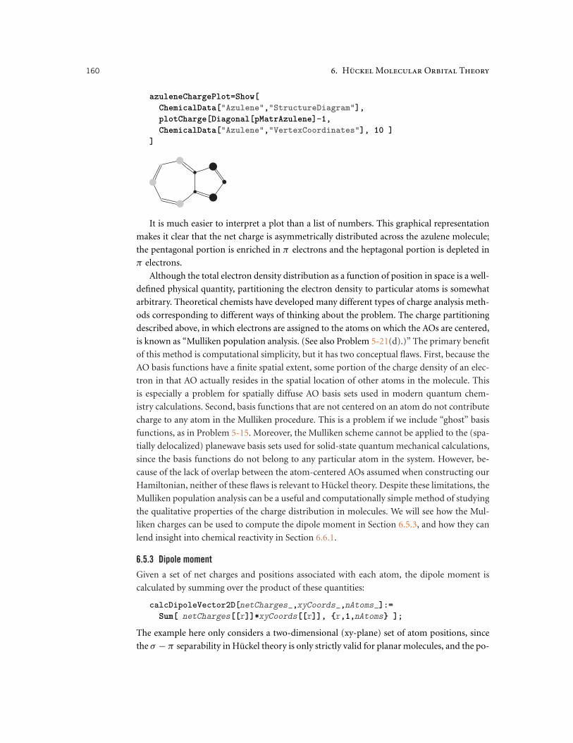
azuleneChargePlot=Show[

ChemicalData["Azulene","StructureDiagram"],

plotCharge[Diagonal[pMatrAzulene]-1,

ChemicalData["Azulene","VertexCoordinates"], 10 ]

]

It is much easier to interpret a plot than a list of numbers. This graphical representation

makes it clear that the net charge is asymmetrically distributed across the azulene molecule;

the pentagonal portion is enriched in π electrons and the heptagonal portion is depleted in

π electrons.

Although the total electron density distribution as a function of position in space is a well-

defined physical quantity, partitioning the electron density to particular atoms is somewhat

arbitrary. Theoretical chemists have developed many different types of charge analysis meth-

ods corresponding to different ways of thinking about the problem. The charge partitioning

described above, in which electrons are assigned to the atoms on which the AOs are centered,

is known as “Mulliken population analysis. (See also Problem 5-21(d).)” The primary benefit

of this method is computational simplicity, but it has two conceptual flaws. First, because the

AO basis functions have a finite spatial extent, some portion of the charge density of an elec-

tron in that AO actually resides in the spatial location of other atoms in the molecule. This

is especially a problem for spatially diffuse AO basis sets used in modern quantum chem-

istry calculations. Second, basis functions that are not centered on an atom do not contribute

charge to any atom in the Mulliken procedure. This is a problem if we include “ghost” basis

functions, as in Problem 5-15. Moreover, the Mulliken scheme cannot be applied to the (spa-

tially delocalized) planewave basis sets used for solid-state quantum mechanical calculations,

since the basis functions do not belong to any particular atom in the system. However, be-

cause of the lack of overlap between the atom-centered AOs assumed when constructing our

Hamiltonian, neither of these flaws is relevant to Huckel theory. Despite these limitations, the

Mulliken population analysis can be a useful and computationally simple method of studying

the qualitative properties of the charge distribution in molecules. We will see how the Mul-

liken charges can be used to compute the dipole moment in Section 6.5.3, and how they can

lend insight into chemical reactivity in Section 6.6.1.

6.5.3 Dipole moment

Given a set of net charges and positions associated with each atom, the dipole moment is

calculated by summing over the product of these quantities:

calcDipoleVector2D[netCharges_,xyCoords_,nAtoms_]:=

Sum[ netCharges[[r]]*xyCoords[[r]], {r,1,nAtoms} ];

The example here only considers a two-dimensional (xy-plane) set of atom positions, since

the σ − π separability in Huckel theory is only strictly valid for planar molecules, and the po-


sitions specified by VertexCoordinates are only given in two dimensions.11 Even with the

“correct” positions, the dipole moments calculated within Huckel theory are at best qualita-

tive, since the σ electrons and distortions of the molecule by the uneven charge distribution

(both ignored by the underlying assumptions) play an important role. As a concrete example,

let us calculate the dipole moment vector and its magnitude for azulene:

azuleneDipole=calcDipoleVector2D[ Diagonal[pMatrAzulene]-1,

ChemicalData["Azulene","VertexCoordinates"], 10 ]

dipoleMoment=Sqrt[azuleneDipole.azuleneDipole] (* units of charge/pm *)

{95.7645, 0.476481}

95.7657

Based on the azulene net charge distribution plot in Section 6.5.2, and the symmetry of the

molecule, the 0.47 component of the azuleneDipole vector seems suspect; there is no rea-

son to expect any such asymmetry. However, this is less than half a percent of the other value,

and arises from numerical round-off of the charges and positions rather than a physically

meaningful asymmetry. Nevertheless, it is clear that azulene has a dipole moment. Note that

a dipole moment has units of charge/length. The “length” is whatever units VertexCoordi-

nates uses, so be careful in your physical interpretation and unit conversion.12

The orientation of the dipole moment is more easily interpreted as a picture. For example,

to draw a vector as a Green Arrow[] centered at the geometric center of the molecule, and

pointing along a specified direction, we could define the function

plotDipoleVector2D[dipoleVec_,xyCoords_,nAtoms_]:=

Graphics[ {Thick, Green, Arrowheads[.1],

Arrow[{Mean[xyCoords]-dipoleVec/2,Mean[xyCoords]+dipoleVec/2}]} ];

and combine it with a plot of the azulene molecule StructureDiagram using the Show[]

function:

Show[


plotDipoleVector2D[azuleneDipole,

ChemicalData["Azulene","VertexCoordinates"],10 ] ]

The insignificance of the 0.47 component is clear when plotted in this way.

11. For nonplanar molecules, VertexCoordinates corresponds to the 2D organic-chemistry-type diagramreturned by StructureDiagram, which is an arbitrarily distorted (nonmetric-conserving) projection ontothe xy-plane. This is a fancy way of saying that the 2D diagram doesn’t correspond to anything particularlyphysical about the 3D structure of the molecule, aside from preserving the Lewis-bond connectivity. This isjust the regular practice of drawing 3D molecules in 2D that you see in every organic chemistry textbook.12. To do this correctly, you should work in 3D and use the AtomPositions property in ChemicalData[],which gives the 3D position in units of picometers. But this level of quantitative accuracy is unwarrantedgiven the limitations of Huckel theory and the Mulliken population analysis.


6.5.4 Bond order/length/strength

What about the off-diagonal entries in the charge density matrix? These can be interpreted

as the bond order between atoms. As you will recall from introductory chemistry, bond order

generalizes the idea of “single,” “double,” and “triple” bonds from Lewis theory to a contin-

uum of possible values. Moreover, bond order serves as a link between the “strength” (bond

dissociation energy) and length of the bond: (i) the higher the bond order, the stronger the

bond; (ii) the stronger the bond, the shorter the bond. This bond-order/length/strength rela-

tionship allows us to gain insight into the relative bond lengths and strengths in the molecule.

Since the Huckel Hamiltonian considers only π electrons, these results only describe the π-

electron bond order. Though the σ bond order is not described by this Hamiltonian, σ bonds

are localized and are only weakly affected by the molecular context in which they occur. To a

first approximation, all σ bonds between carbon atoms have about the same energy. In con-

trast, since the π orbitals are delocalized over the molecule, the π bond order depends on the

total molecular environment, and it is precisely this influence that we seek to understand.

The bond order matrix is defined as the elements of the charge density matrix corre-

sponding to the nearest-neighbor bonds between atoms. You could simply read the entries

contained in the full charge density matrix, but it also contains lots of terms that do not cor-

respond to “bonds between atoms” as they would be understood relative to Lewis structures.

Taking advantage of the fact that the Huckel Hamiltonian has only nonzero entries at exactly

these nearest-neighbor bond positions,13 we will remove these additional terms by perform-

ing an element-by-element multiplication of the charge density and Hamiltonian matrices:

ChemicalData["Benzene"]

MatrixForm[

SetPrecision[nnBOMatrBenzene=pMatrBenzene*Unitize[hMatrBenzene], 2] ]

Note that the asterisk operator (*) is not matrix-matrix multiplication; rather, it proceeds

element by element through the matrices (which are both the same size), and computes a

new matrix by multiplying each particular element by the corresponding element in the other

matrix.

13. With the exception of on-site terms in heteroatomic aromatic molecules, e.g., those in Section 6.4, wherethere would also be diagonal elements to be removed.


Similarly, the bond order matrix for azulene can be computed by


MatrixForm[

SetPrecision[nnBOMatrAzulene=pMatrAzulene*Unitize[hMatrAzulene], 2] ]

All of the bonds in benzene have a greater bond order than any of the bonds in azulene,

suggesting that the aromatic bonds in benzene are more stable than those in azulene (greater

bond order implies greater bond strength). Furthermore, all of the bonds in benzene are

the same (equal bond order implies equal bond length), as expected from the molecular

symmetry. In contrast, the bonds in azulene seem to vary, suggesting that some of the bonds

are shorter or longer than others. A comparison to the bond orders in benzene suggests

that the azulene C-C bonds are all about the same or longer than the C-C bond lengths in

benzene. As before, it is convenient to plot the results. The strategy is basically the same as

in the previous examples of the molecular orbital and charge density plotting functions from

Sections 6.5.1 and 6.5.2, except that each Disc[] is placed between two atom positions rather

than centered on an atom.

plotBondOrders[nnBondOrderMatr_,xyCoords_,nAtoms_]:=Module[

{graphicsList={}},

Do[

AppendTo[graphicsList,Orange];

AppendTo[graphicsList,Opacity[0.5]];

AppendTo[graphicsList,

Disk[ Mean[{xyCoords[[r]], xyCoords[[s]]}],

N[scaledRadius[1.6, Abs[nnBondOrderMatr[[r,s]] ]]]]];

,{r,1,nAtoms-1},{s,r+1,nAtoms}];

Graphics[graphicsList]

];

Plotting the bond orders in azulene,

Show[


plotBondOrders[nnBOMatrAzulene,

ChemicalData["Azulene","VertexCoordinates"], 10] ]


one sees that the bond lengths tend to alternate slightly longer and shorter than average as

one proceeds around the ring, and that the vertical C-C bond shared by the heptagon and

pentagon rings has the lowest bond order, and is thus predicted to be the weakest and the

longest bond in the molecule. How does this compare to experiment or ab initio (i.e., “first-

principles”) calculations?

6.6 MOLECULAR REACTIVITY

Within the Born-Oppenheimer approximation, a “molecule” is just a local minimum of the

total energy, as a function of the spatial arrangement of a collection of nuclei with a certain

number of electrons. The energy of the collection of nuclei and electrons as a function of

their relative positions defines the potential energy surface. If there are N atoms, each located

in a three-dimensional space, then there are roughly 3N dimensions in the potential energy

hypersurface (a few less, depending on the symmetry of the molecules and removing the

center of mass motion of the system). Different electronic states of the molecule have different

potential energy surfaces. “Chemical reactions,” then, are simply transitions between local

minima on these high-dimensional potential energy surfaces. The rates at which transitions

occur (i.e., the reaction kinetics) can be computed using the toolbox of chemical dynamics

theory—the simplest example being classical transition state theory, but more exact methods

that take into account the quantum nature of particles (and factors such as tunneling) are also

used. The “reaction coordinate,” discussed in the typical introductory chemistry treatment of

transition state theory, corresponds to a line between a particular “reactant” and “product”

arrangement in this high-dimensional space. Since the lowest-barrier paths are the fastest

(and hence contribute most to the rate), this reaction coordinate path is chosen to do the

least amount of “hill climbing” along the way from reactants to product. Saddle points along

this reaction coordinate correspond to the “transition state” arrangements. Basins (i.e., local

minima) along this path correspond to reactive intermediates. In this way, the solution to the

electronic Schrodinger equation provides a complete understanding of chemical reactivity.

In practice, this is rather challenging. First, calculating the potential energy surface is

computationally expensive. Second, to have physical meaning, the barrier heights must be

quite accurate, since these appear in an exponential when computing the Boltzmann factors.

Consider the numerical errors seen in previous exercises in this book, relative to kBT ≈10−3 Eh at room temperature. Third, chemical dynamics theory requires a combination of

statistical mechanics and quantum mechanics that may be out of the scope of your present

coursework. So while this comprehensive theory for computing chemical reaction rates is

plausible, the calculations are beyond the scope of this book.

An alternative theory of reactivity is to consider the propensity of certain initial states

toward chemical reactions. This is much simpler, since it only requires computing a single

6.6 molecular reactivity 165

point (i.e., just one molecule, in one particular initial “reactant” state) on the potential energy

surface. In practice, this tends to accurately identify the relative reactivities of different parts

of the molecule, though without the information of the energy along the reaction coordinate

it does not give quantitative rate predictions.

Organic reactions may be broadly classified into three types: polar, nonpolar, and per-

icyclic. In polar reactions, a new bond is formed when a nucleophile provides a pair of

electrons to an electrophile. An electrophilic (“electron-loving”14) reagent is “attracted” to

electrons, and participates in the chemical reaction by accepting an electron pair (i.e., as a

Lewis acid). Consequently, electrophiles are expected to attack the most electron-rich part of

the target molecule, i.e., the region of the target molecule that is best able to provide electrons.

A nucleophilic (“nucleus-loving”) reagent donates electrons, and is thus a Lewis base. Conse-

quently, nucleophiles will attack the most electron-poor part of the target molecule, i.e., the

region of the target molecule that is best able to accept the electrons that are being donated.

As seen earlier in the chapter, the charge distribution can be calculated using Huckel theory,

suggesting that the results can be used to predict these reactive sites. Nonpolar reactions oc-

cur when both species contribute electrons “equally” to the new bond. The classic example of

these are radical reactions, and this property can be described using the free valence index in-

troduced in Section 6.6.3. Finally, pericyclic reactions are concerted processes involving cyclic

transition states where the electrons simultaneously break and form bonds. The classic exam-

ples of pericyclic reactions are electrocyclic reactions and Diels-Alder cycloaddition reactions.

These can be understood in terms of the difference between the HOMO and LUMO energies

and the relative phases of the π molecular orbitals.

6.6.1 Charge density and polar reactions

As discussed above, electrophilic reagents are expected to attack the most electron-rich re-

gions of the target molecule and nucleophilic reagents are expected to attack the most

electron-poor regions of the target molecule. The net charge on each atom (discussed in

Section 6.5.2) quantifies how “rich” or “poor” a site is. If a particular atomic site has more

electrons located on it (as given by the charge density matrix) than the neutral atom, it has a

net negative charge and will be more susceptible to electrophilic attack. If the site is electron

poor, it will have a net positive charge.

Consider the napthalene, azulene, aniline, and benzaldehyde molecules. Construct the ap-

propriate molecular Hamiltonians, determine the eigensolutions, and then create the charge

density plot. I’ll let you do this as an exercise, and just show the result of these plots here:

(* Generate a charge density matrix and use it to construct a

benzaldehydeChargePlot on your own before continuing. *)

GraphicsGrid[{

{"Naphthalene",naphthaleneChargePlot},

{"Azulene",azuleneChargePlot},

14. The sense of “love” in this case is somewhere between the theories presented by Aristophanes, Agathon’sconcessions to Socrates’s questioning, and the theory of Diotima related by Socrates in Plato’s Symposium.


{"Aniline",anilineChargePlot},

{"Benzaldehyde",benzaldehydeChargePlot} }]

Notice how naphthalene has a uniform charge density; the charge density–based initial

state theory of reactivity does not give any information about reactivity (this is resolved in

the next section). Azulene has a clear preference for electrophilic attacks on the pentagon and

nucleophilic attacks on certain sites of the heptagon. The amine group in aniline strongly

activates the ring toward electrophilic reaction by pushing electron density into the ortho

and para sites of the benzene ring. Conversely, the carbonyl group in benzaldehyde is a

deactivating group. By withdrawing electron density from the ring, particularly from the

ortho and para sites, it makes those sites less susceptible to electrophilic aromatic substitution

reactions. Consequently, the meta positions are the least deactivated (they still have the full

number of electrons that an isolated carbon atom has), and thus carbonyl is described as a

meta-directing group. In this way, the patterns of ortho-para-activation by electron-donating

groups and meta-direction by electron-withdrawing groups are a simple consequence of the

π electronic structure. While it is easy to memorize these types of rules for single rings, Huckel

theory allows us to calculate how these directing groups behave in polycyclic aromatics.

Organic chemists tend to enjoy these types of calculations.

6.6.2 Frontier molecular orbitals and polar reactions

Contrary to the charge-density analysis predictions of the previous section, experiment indi-

cates that the positions in naphthalene are not equally reactive. This is a general problem for


most unsubstituted aromatic hydrocarbon molecules,15 resolved by the Nobel Prize–winning

insights of Kenichi Fukui that one must also consider the role of the highest-occupied and

lowest-unoccupied molecular orbitals in the bonding process.16 These molecular orbitals are

referred to as the “frontier” molecular orbitals, since they are at the boundary of the occu-

pied and unoccupied molecular orbital states. If the electron density is uniform in all sites

(i.e., all else being equal), then taking the electron from the highest-occupied molecular or-

bital (HOMO) changes the total energy by the least amount. The sites where the HOMO

density (i.e., |ψ |2) is largest indicate locations with the highest relative propensities for this

reaction. Similarly, when extra electrons are added to the molecule, they will be placed into

the lowest-unoccupied molecular orbital (LUMO). Regions where the LUMO density is low-

est thus correspond to addition sites that induce the least total energy change.

Returning to the specific case of naphthalene, although the charge density is predicted to

be uniform for all the sites, the HOMO and LUMO orbitals are not:

evalsNaphthalene

GraphicsGrid[

Prepend[

Table[

{evalsNaphthalene[[i]], Show[

ChemicalData["Naphthalene","StructureDiagram"],

plotMO[i,ChemicalData["Naphthalene","VertexCoordinates"],

evecsNaphthalene,10] ]},

{i,6,5,-1}],

{"Energy/eV","MO Diagram"}] ]

{-6.21749, -4.36869, -3.51749, -2.7,

-1.66869, 1.66869, 2.7, 3.51749, 4.36869, 6.21749}

15. Specifically, alternant hydrocarbons all have uniform charge density in Huckel theory. An alternanthydrocarbon is one in which neighboring sites can be labeled as “a” or “b” in alternating sequence, withoutever having an “aa” or “bb” nearest neighbor. You can see this yourself by trying to label naphthalene orbenzene (both alternant hydrocarbons) versus azulene (a nonalternant hydrocarbon).16. K. Fukui, T. Yonezawa, H. Shingu, “A Molecular Orbital Theory of Reactivity in Aromatic Hydrocarbons,”J. Chem. Phys. 20, 722–725 (1952), http://dx.doi.org/10.1063/1.1700523.

http://dx.doi.org/10.1063/1.1700523


The nodes on the bridging carbons indicate that these will be the least reactive. Since the

reagent only cares about the magnitude of the wavefunction coefficient and not the sign, it is

clearer to represent |ψ |2 for these frontier MOs:

GraphicsGrid[

Prepend[

Table[

{evalsNaphthalene[[i]],

Show[

ChemicalData["Naphthalene","StructureDiagram"],

plotMO[i,ChemicalData["Naphthalene","VertexCoordinates"],

evecsNaphthalene^2,10] ]},

{i,6,5,-1}],

{"Energy/eV","|ψ|2" Diagram}] ]

This plot shows that the reactivity pattern of naphthalene toward electrophilic and nucle-

ophilic reagents is spatially the same. The α carbons (closer to the middle) are predicted to

have higher reactivity than the β carbons (furthest from center), and the bridging carbons are

predicted to be unreactive. Thus, despite the uniform electron density, the spatial distribution

of the molecular orbitals determines the reactivity patterns of molecules.

6.6.3 Free valence index and radical attack

The free valence index measures the degree that atoms in a molecule are bonded to adjacent

atoms relative to a maximum theoretical bonding power. The free valence index for a partic-

ular atom, r , is defined as

Fr = Nmax −∑

s∈n .n .(r)

Prs , (6.7)


where the sum is performed over other atoms, s, that are nearest neighbors (connected by

a “bond”) of atom r . The maximum π bond order for a carbon atom is Nmax = √3.17 The

carbon atom with the largest free valence index has the greatest propensity to radical attack.

We can rationalize this in the following way: To bond with the radical, the atom must “give

up” one electron. If the adjacent bonds already have a claim on the electron, it will not be

available for the new bond with the radical. The free valence index thus measures the amount

of that atom’s electron that is not already participating in chemical bonding (as measured by

the bond order entries, Prs).

The free valence index can be easily computed using the bond order matrices calculated

in Section 6.5.4. In constructing the bond order matrix, only the nearest-neighbor terms

remain. Thus, summing over a particular row (or column) corresponding to atom r will

give the sum needed for Eq. (6.7). Fr (Eq. (6.7)) is evaluated for each atomic site, r, using

a Table[] function that loops over the atom indices. For example, using the bond order

matrix of benzene (nnBOMatrBenzene) defined in Section 6.5.4,

benzeneFreeValence=Table[

Sqrt[3]-Sum[nnBOMatrBenzene[[r,s]],{s,1,6}]

,{r,1,6}]

{0.398717, 0.398717, 0.398717, 0.398717, 0.398717, 0.398717}

all of the Fr values are identical, in contrast to azulene,

azuleneFreeValence = Table[

Sqrt[3]-Sum[nnBOMatrAzulene[[r,s]],{s,1,10}]

,{r,1,10}]

{0.149677, 0.149677, 0.48038, 0.48038,

0.482214, 0.482214, 0.419972, 0.429112, 0.429112, 0.454253}

in which the atoms have different values of Fr and hence different propensities to radical at-

tack. The positions with greater values of Fr can be visualized by utilizing the plotCharge[]

function, previously defined in Section 6.5.2, to overlay the list of Fr values contained in

azuleneFreeValence on top of the structure of the azulene molecule:

Show[


plotCharge[azuleneFreeValence,

ChemicalData["Azulene","VertexCoordinates"],10] ]

17. An alternative definition uses the total bond order, i.e., for a π-bonded carbon atom this would consistof three σ bonds plus the π bond for a total of Nmax = 3 + √

3. Similarly, then, the bond order sum wouldbe expanded to include each of the σ bonds, which would nominally be 3 (one for each of the σ bonds).


6.6.4 Orbital symmetry conservation in pericyclic reactions

The Woodward-Hoffmann rules and Diels-Alder reactions rely on the conserved symmetry of

the various ring-opening and ring-closing reactions. The basic principle in these pericyclic re-

actions is phase (sign of the wavefunction) matching of the various components. The required

phase matching then enforces a constraint on whether the rotation will occur in a conro-

tatory or disrotatory fashion, ultimately leading to different stereochemical consequences.18

The techniques described in Section 6.3.3 can be used to make diagrams for your own mol-

ecules. Although the π-electron theory discussed in this chapter is often a good start, rotations

of the bonds induce σ–π mixing, breaking the assumed neglect of these AOs. We will not

discuss pericyclic reactions in depth here, but for further reference see the following sources:

. R. B. Woodward and R. Hoffmann, The Conservation of Orbital Symmetry (Wein-

heim/Bergstr.: Verlag Chemie, 1970)

. Keith Yates, Huckel Molecular Orbital Theory (New York: Academic Press, 1978)

6.6.5 Limitations of Huckel theory for chemical reactivity

Although Huckel theory is convenient for illustrating basic quantum theories of chemical

reactivity, many other factors contribute to the outcome of reactions. For example, the cal-

culations discussed above do not account for steric contributions that alter the likelihood of

specific reactions occurring. Using only the initial molecular states ignores the details of the

potential energy landscape; thus it cannot account for cases where the outcome of reactions

is determined by kinetic factors. Restricting ourselves to the π-electron Hamiltonian, effects

of σ -π mixing are ignored. Moreover, the extremely simplified Hamiltonian—particularly

the complete neglect of electron-electron interactions—precludes incorporating many other

factors, such as the effects of solvent polarity. Yet despite these limitations, Huckel theory

makes surprisingly accurate predictions for aromatic hydrocarbon reactivity, and thus can

still provide a conceptual framework for understanding chemical reactions. This is valuable

for explaining your work to others (and yourself!), and can be substantiated with more quan-

titatively accurate ab initio calculations.

6.7 LOOKING FORWARD

Huckel theory’s underlying approximations (described in Section 6.1.2) limit the types of

molecules and properties that can be described and the accuracy of those predictions. Re-

moving these simplifying approximations—by including electron-electron interactions and

σ electrons—provides a path toward predicting molecular structure, spectroscopy, and reac-

tivity for all molecules. We’ll conclude the chapter with a brief discussion of semiempirical

electronic structure theories that implement intermediate approximations, followed by an

18. R. B. Woodward and R. Hoffmann, “Orbital Symmetries and endo-exo Relationships in ConcertedCycloaddition Reactions,” J. Am. Chem. Soc. 87, 395–397 (1965), http://dx.doi.org/10.1021/ja00947a033.

http://dx.doi.org/10.1021/ja00947a033

6.7 looking forward 171

overview of the role of electronic structure calculations in the theory of molecular property

prediction.

6.7.1 Beyond pi-electron theory

Neglecting the Coulomb and exchange interactions is an extreme approximation, with the

consequence of removing the difference between singlet and triplet electronic states. In addi-

tion, there is more to chemistry than planar aromatic hydrocarbons. How can we go beyond

these limitations without going back to the full Hartree-Fock theory discussed in Chapter 5?

One way is to include the Coulomb and exchange interactions in an approximate way.

One class of theories (e.g., the Parr-Parriser-Pople theory, the Hubbard model) extend the

π-electron theory for planar hydrocarbons by adding Coulomb and exchange integrals (de-

scribed as parameterized functions). The parameters of the Coulomb and exchange inte-

gral functions are derived from spectroscopic or thermodynamic experiments, like the one-

electron integrals used here, and the functions represent the average behavior of the integral

between the various carbon 2pz orbitals. By including the Coulomb and exchange integrals,

one can carry out a semiempirical Hartree-Fock calculation, analogous to the hydrogen mol-

ecule calculations in Section 5.2. Because the integrals are approximated as simple functions

of distance, they can be calculated rapidly. Inclusion of the Coulomb and exchange terms al-

lows for a more accurate description of the charge distribution, and allows for different spin

states. Unfortunately, though, this requires an iterative SCF calculation rather than the simple

“one-shot” calculations performed in this chapter. Another benefit is that the two-electron

integrals can be used to perform configuration-interaction calculations that go beyond the

mean field Hartree-Fock scheme. That being said, these theories are still limited to the π-

electronic structure of planar aromatic molecules.

Another strategy for improving Huckel theory is by including the other valence electron

orbitals, while still assuming that the core electrons do not participate in bonding. One ex-

ample is the “extended” Huckel theory (EHT), which includes not only the 2pz orbitals on

the carbons, but all the other valence atomic orbitals on all the atoms (including hydro-

gens). The Hamiltonian is constructed in a similar way as above, but with the use of certain

distance-dependent rules to compute the Hamiltonian matrix elements, e.g., scaling them by

a function of the overlap between the valence atomic orbital functions. Conceptually, this only

adds the complications of dealing with 3D geometries and the additional parameters describ-

ing the integrals between the many basis functions on each atom. The principal advantage

over Huckel theory is that geometric effects such as bond-length changes and nonplanarity

are now included in the Hamiltonian. Like Huckel theory, there are no Coulomb or exchange

integrals in EHT, so it shares the same limitations with respect to the self-consistency of

the charge distribution, lack of distinction between singlet and triplet states with the same

molecular orbital occupation, etc. The natural next step is to account for the interactions by

including Coulomb and exchange terms (again, in the form of semiempirical functions fitted

to reproduce experimental data), yielding the various families of semiempirical Hartree-Fock

methods—e.g., CNDO, ZINDO, AM1, MNDO, PM3, PM6, PM7. With some clever matrix


manipulations and numerical tricks, these semiempirical methods can be scaled up to per-

form quantum calculations on small proteins.

Historically, the development of these semiempirical techniques was motivated by the

high computational cost of performing full ab initio Hartree-Fock calculations using large

basis sets. However, improvements in computer hardware and algorithms have made ab initio

Hartree-Fock and even post-Hartree-Fock corrections computationally unremarkable for

even somewhat large (50–100 atom) systems. Of course, “feasible” depends on your definition

of what a “large” molecule is, what a “good enough” basis set is, how “fast” you want your

results, and how “fast” your computer is. Semiempirical molecular orbital theories might

still be the only appropriate tool for treating large nanostructures containing more than 103

atoms, or computing the many thousands of points needed for the potential energy surface

(indeed, if our calculations are fast enough, we might consider computing the potential

energy surface “on the fly”). From a conceptual point of view, the simpler theories let us “turn

off” certain interactions in predictable ways, and perhaps give us insight into the properties

of molecules.

6.7.2 Understanding molecular spectroscopy and reactivity from electronic structure

The choice of model chemistry provides an approximate solution to the electronic structure

problem, with varying trade-offs between computational feasibility and accuracy. The Huckel

model used in this chapter provides a simple means of performing electronic structure cal-

culations that are amenable to a quick, pedagogical examination. In principle, Hartree-Fock

calculations (Chapter 5), post-Hartree-Fock methods (Section 5.3.1), density functional the-

ory methods (Chapter 8), or quantum Monte Carlo methods (Chapter 9) could all be used

instead for more accurate (but more time-consuming) predictions. The same type of analy-

sis of molecular properties and reactivity can be undertaken with these more sophisticated

methods. For example, going beyond the π-electron theory allows the role of sigma-bonding

electrons in molecular properties and reactivity to be calculated. The total energy of the sys-

tem can be minimized by moving the atoms around (similar to Section 5.2.7, although now

with 3N possible choices rather than just a single internuclear distance). If you want to deter-

mine the energy change as you move a particular atom, reach in to your simulation and move

it! This gives us a new way to study chemical reaction mechanisms by explicitly computing

various hypothetical reaction paths. For an overview of this field, see Bachrach’s textbook.19

The reader with a background in statistical mechanics will realize that this provides a

toolbox for calculating all the possible vibrational, rotational, and electronic states, which

may then be used to construct a partition function for computation of all the thermodynamic

properties for noninteracting systems. (See also Appendix D.) For interacting (nonideal gas

systems or condensed phases), the intermolecular interactions20 can be calculated and used

19. Steven M. Bachrach, Computational Organic Chemistry, 2nd ed., (Hoboken: Wiley-Interscience, 2014).20. At least the simple electrostatic ones like dipole-dipole interactions, and hydrogen bonding. The disper-sion forces arise from electron correlation, necessitating a post-Hartree-Fock theory.

problems 173

to approximate the partition function by Metropolis Monte Carlo sampling (discussed in

Chapter 11). In this way, electronic structure calculations provide a formal basis for molecular

spectroscopy, reactivity, and thermodynamics.

PROBLEMS

6-1. Which is more stable, phenanthrene or anthracene? Both have the same number of

σ bonds, so the difference is due to aromatic stabilization. Because the electrons are non-

interacting, the total π contribution to the total energy is simply the sum of the occupied

eigenstates,

Eπtotal = 2

Nocc∑i=1

Eπi

, (6.8)

where Eπi

is the energy of the ith MO. (The factor of two comes from each state being doubly

occupied.) Use this equation to determine which molecule has the lowest total energy, i.e., is

the most thermodynamically stable.

6-2. An alternative expression for the π contribution to the total energy is

Eπtotal =

Nbasis∑r=1

Prrαr + 2

Nbasis∑r=1

Nbasis∑s>r

Prsβrs , (6.9)

where Prs are the elements in the charge density matrix from Section 6.5, αr is the on-site

Hamiltonian matrix element for atom r , and βrs is the nearest-neighbor coupling Hamil-

tonian matrix between atoms r and s. Calculate the total energies of phenanthrene and an-

thracene and compare to the values you found in the previous problem. (This is one way to

double-check your calculations.)

6-3. Biphenyl consists of two connected phenyl rings that are rotated relative to each other by

an angle θ . While Huckel theory does not account for steric energy contributions, the effect of

this twist on the π molecular orbital structure can be modeled by setting the nearest-neighbor

Hamiltonian matrix element for the bond between the two rings to t cos θ , where t is the usual

carbon-carbon interaction introduced in Section 6.2. Plot Eπtotal (Eq. (6.8)) as a function of θ .

Given that the experimental equilibrium torsional angle is θ = 44.4◦, comment on the relative

roles of steric interactions and π conjugation on the total energy (and hence the geometry).

6-4. Terphenyl (also known as diphenylbenzene or triphenyl) consists of a central benzene

ring with two phenyl substituents. Using Huckel theory, compare the total π energy of ortho-,

meta-, and para-terphenyl and predict the relative abundance of the three isomers. (For

simplicity, assume that these are planar.) Calculate the lowest-energy π transitions for each

species, and comment on how they might be distinguished by UV/vis spectroscopy.


Figure 6.1. “Trapezoid” and “triangle” graphene nanoparticles withnonbonding MOs.

6-5. Nonbonding molecular orbitals. In the text, we have seen examples of bonding MOs

(with energies lower than the parent AOs) and antibonding MOs (with energies higher than

the parent AOs). However, it is also possible to have “nonbonding” MOs, which are linear

combinations with the same energy as the parent AOs. The “triangle” and “trapezoid” pol-

yaromatic hydrocarbons shown in Figure 6.1 are two examples of molecules with nonbonding

π MOs.21 Using Huckel calculations, determine the number of nonbonding MOs for these

two molecules. You will have to build the Huckel matrix by hand since these molecules aren’t

in the ChemicalData[] database. (Hint 1: It is easy to make mistakes; one sanity check is to

verify that your matrix is Hermitian. Hint 2: Use Chop[] to turn numerical values that are

very close to zero (in this case on the order of 10−16) into “zeros” when counting them.)

6-6. Lycopene is a carotenoid pigment found in many foods, such as tomatoes and

watermelon. Perform a Huckel calculation for lycopene (C40H56), and calculate the HOMO-

LUMO gap. What color does Huckel theory predict? (Hint 1: Not all the carbons are part of

the π-electron system; only carbons that are part of the π system should be described in your

Huckel Hamiltonian. Hint 2: Use a color wheel to identify complementary colors.)

6-7. Acidity and basicity. Adding a proton to a base can be considered as a chemical reaction

that converts the molecule from X to XH+. The change in energy, E = EXH+ − EX, is thus

proportional to the equilibrium constant for the reaction, as measured by the pKa.

(a) Protonation of a nitrogen atom in a heterocyclic base changes the nitrogen atom

types from pyridine-like (N) to pyrrole-like (N+), requiring changes in the on-site

and off-diagonal Hamiltonian matrix elements. Calculate the change in the π energy

and rank the following molecules from lowest pKa to highest: acridine, isoquinoline,

pyridine, quinoline.

21. P. Potasz, A. D. Gluclu, P. Hawrylak, “Zero-Energy States in Triangular and Trapezoidal GrapheneStructures,” Phys. Rev. B 81, 033403 (2010), http://dx.doi.org/10.1103/PhysRevB.81.033403.

http://dx.doi.org/10.1103/PhysRevB.81.033403

problems 175

(b) A “rule of thumb” that can be derived from Huckel theory22 is that the change

in energy—and hence the pKa—is proportional to the charge on the nitrogen atom.

Using the charge density matrix for the molecules in the previous part, rank them

from lowest pKa to highest. How does this compare to your previous result?

6-8. Experimentally, 6,6-diphenyl-fulvene has a larger dipole moment than 6,6-bis-

(p-chlorophenyl)fulvene.23 Using Huckel calculations, calculate the dipole moments of these

species. (Hint: The former is available as ChemicalData["Diphenylfulvene"]; you’ll have

to build the latter yourself, being sure to incorporate the correct chlorine matrix elements

from Table 6.1.)

6-9. The infrared N-H stretching frequency for primary aromatic amines is proportional to

the electron density on the nitrogen atom.24 Rank the following molecules in terms of their

predicted N-H stretching frequencies: aniline, ortho-chloroaniline, meta-chloroaniline, para-

chloroaniline.

6-10. The infrared C-H stretching frequency correlates with the free valence index on the

carbon atom.25 Rank the different C-H stretching frequencies for the unique sites in the

styrene molecule.

6-11. Using the bond-order/length/strength relationship, predict the relative bond lengths for

all of the (unique) C-C bonds in biphenylene.

6-12. The infrared C=O stretching frequency can be predicted by using the bond-order/

length/strength relationships in Section 6.5.4. Higher C=O bond order corresponds to

“stiffer” bonds with higher C=O vibrational frequency, and lower C=O bond order corre-

sponds to “looser” bonds with lower C=O vibrational frequency.

(a) Using the C=O bond order, rank these molecules for increasing carbonyl stretching

frequency: acrolein, benzaldehyde, benzophenone, formaldehyde.

22. H. C. Longuet-Higgins, “Some Studies in Molecular Orbital Theory II. Ionization Constants inHeteroaromatic Amines and Related Compounds,” J. Chem. Phys., 18, 275–282 (1950), http://dx.doi.org/10.1063/1.1747619; in fact, this paper takes it one step further and relates the basicity to the charge on thecorresponding nonheteroatomic aromatic hydrocarbon. Back when all these calculations needed to be doneby hand, there was a strong motivation not to perform new calculations! However, the relationship betweenincreasing nitrogen charge and increasing pKa is more rigorous, and holds even for more sophisticated all-electron Hartree-Fock and density functional theory calculations, e.g., S. R. A. Leite, “Basicities of PrimaryArylamines and Calculated Amine Nitrogen Electronic Charges,” Ecl. Quim. (Sao Paulo) 23, 71–80 (1998),http://dx.doi.org/10.1590/S0100-46701998000100006.23. G. W. Wheland and D. E. Mann, “The Dipole Moments of Fulvene and Azulene,” J. Chem. Phys. 17,264–268 (1949), http://dx.doi.org/10.1063/1.1747237.24. S. F. Mason, “The Frequencies and Intensities of the N–H Stretching Vibrations in Primary Amines,”J. Chem. Soc. 3619–3627 (1958), http://dx.doi.org/10.1039/JR9580003619.25. G. M. Badger and A. G. Moritz, “The C-H Stretching Bands of Methyl Groups Attached to Poly-cyclic Aromatic Hydrocarbons,” Spectrochim. Acta 15, 672–678 (1959), http://dx.doi.org/10.1016/S0371-1951(59)80363-5.

http://dx.doi.org/10.1063/1.1747619

http://dx.doi.org/10.1590/S0100-46701998000100006

http://dx.doi.org/10.1063/1.1747237

http://dx.doi.org/10.1039/JR9580003619

http://dx.doi.org/10.1016/S0371-1951(59)80363-5


(b) Is it possible to distinguish between 1-naphthaldehyde and 2-naphthaldehyde

based solely on the C=O stretching frequency?

(c) Modify the benzaldehyde Hamiltonian to investigate the effect of substituting a

chlorine atom in the ortho, meta, and para positions relative to the carbonyl group.

Order your predicted carbonyl stretching frequencies, and compare to experiment.

(d) Put a carbonyl group on the end of a pi-conjugated chain of carbon atoms (e.g.,

ethylene, butadiene, hexatriene, octatetraene). How does the carbonyl stretching fre-

quency change as a function of the length of the pi-conjugated chain?

6-13. At what positions would you expect nucleophilic, electrophilic, and radical attacks to

occur in phenanthrene?

6-14. At what positions would you expect nucleophilic, electrophilic, and radical attacks to

occur in acetophenone?

6-15. Resveratrol is a polyphenol found in grape skins and seeds; it is nearly planar, so assume

that Huckel theory is valid. Where would you expect nucleophilic, electrophilic, and radical

attacks to occur? (Hint: Modify your Hamiltonian to account for the different on-site and

nearest-neighbor matrix elements involving the oxygen atoms, as discussed in Section 6.4.

Also, be sure to count the π electrons correctly.)

6-16. The relative rates of reaction of a trichloromethyl radical toward aromatic hydrocarbons

correlates with the highest free valence index, Fr , of the hydrocarbon—i.e., larger maximum

Fr corresponds to a faster reaction rate.26 Using this principle, rank the following hydrocar-

bons from slowest to fastest reaction with a trichloromethyl radical by using the highest Fr at

any site in the molecule: anthracene, benzene, chrysene, naphthalene, stilbene, phenanthrene.

6-17. Polychlorinated biphenyls (PCBs) are now known as persistent organic pollutants, but

until the 1970s they were widely used in a number of applications due to their high dielectric

constant, thermal conductivity, flashpoint, and relative inertness. PCBs were typically pro-

duced by electrophilic halogenation of biphenyl, resulting in the addition of many chlorines

in many different sites. Use Huckel theory to predict the properties of the PCB mixtures.

(a) Run calculations for planar biphenyl, and biphenyl with a 44.4◦ twist between the

rings (see Problem 6-3). Obtain the charges and frontier molecular orbitals in the two

cases.

(b) Where do you predict the electrophilic addition of the first chlorine atom to occur

on biphenyl, based on your calculations from the previous part? Does the planarity

make a difference? Are there multiple equivalent sites?

(c) Perform Huckel calculations for the monochlorinated biphenyl you predicted in

the previous calculation (again, for both the planar and nonplanar forms). Based on

26. E. C. Kooyman and E. Farenhost, “The Relative Reactivities of Polycyclic Aromatics towards Trichloro-methyl Radicals,” Trans. Faraday Soc. 49, 58–67 (1953), http://dx.doi.org/10.1039/TF9534900058.

http://dx.doi.org/10.1039/TF9534900058

problems 177

the charges and/or frontier MOs, predict the site for the second chlorination. Again,

identify equivalent or nearly equivalent sites, and characterize any differences between

the planar and nonplanar models.

(d) In principle you can continue adding chlorine atoms.27 Repeat the calculations

from the previous steps to determine the most likely positions of the third chlo-

rine atom.

6-18. Hydrocarbon reduction by alkali metals (Birch reduction). When aromatic hydrocar-

bons are put in solution with alkali metals, the dianion of the hydrocarbon is formed. Addi-

tion of a proton source (e.g., an alcohol) results in the addition of two hydrogens. The position

of these additions can be predicted using Huckel theory. For a concrete example, consider the

case of naphthalene.

(a) Naphthalene first gains an electron from the alkali metal. Calculate the charge

density of the molecular anion. (Hint: Be sure to include the singly occupied state

when computing the charges.)

(b) The first proton attacks at the site of the highest electron density of the anion.

Identify this site. (If there are multiple equivalent sites, one is chosen at random.)

(c) After addition of the first proton, the π conjugation of the molecule is disrupted—

the carbon atom to which the first proton was attached now no longer participates in

π bonding. Recalculate the Huckel solution, omitting this carbon atom from your

calculation. This new molecule gains an electron from the alkali metal. Calculate the

charge density of this second molecular anion.

(d) The second proton attacks at the site of the highest electron density of the second

molecular anion (which you calculated in the previous step). Identify this site.

6-19. Carry out the same calculation as in the previous problem, but for reduction of phenan-

threne.

27. In fact, one of the most common PCBs in the United States was Aroclor 1016, a mixture of congenersconsisting of approximately half C12H7Cl3.

introduction to computational physical chemistry · the qualitative model of bonding taught in...

Documents