introduction to aspen plus - beck-shop.de · pdf file2 introduction to aspen plus installation...

CHAPTER ONE

INTRODUCTION TO ASPEN PLUS

Aspen Plus is based on techniques for solving flowsheets that were employed bychemical engineers many years ago. Computer programs were just beginning to beused, were of the stand-alone variety, and were typically used for designing singleunits. The solution of even the simplest flowsheet without recycle required an engineerto design each unit one at a time and, manually, introduce the solution values of apreviously designed unit into the input of the next unit in the flowsheet. When itbecame necessary to deal with a recycle, the calculations began with a guess of therecycle values, and calculations ended when the values produced by the last unit inthe loop matched the guesses. This involved much repetitive work and convergencewas not guaranteed. This procedure evolved through the construction of rating modelsof units, as opposed to design models, which could be tied together by software in away that emulated the procedure above and employed robust mathematical methodsto converge the recycle elements of the process. This type of system is termed asequential modular simulator . An excellent example of such software was MonsantoCorporation’s Flowtran (1974), which eventually became the kernel upon which AspenPlus was built.

Subsequently, Aspen Plus, although still basically a sequential modular simulator,has grown considerably and has many advanced functionalities, such as links to avariety of specialized software, such as detailed heat exchanger design, dynamic sim-ulation, batch process modeling, and many additional functions. It also has a facilityfor using an equation-based approach in some of its models, which permits convenientuse of design specifications in process modeling.

The Aspen Engineering Suite, which incorporates Aspen Plus, can be installedin a variety of ways using network servers or on a stand-alone personal computer.

Teach Yourself the Basics of Aspen Plus™ By Ralph SchefflanCopyright © 2011 John Wiley & Sons, Inc.

1

COPYRIG

HTED M

ATERIAL

2 INTRODUCTION TO ASPEN PLUS

Installation is the responsibility of either the user, with tools provided by Aspen Tech-nology, or the information technology department, which services the user. This is doneonly once and modified, typically annually, with future releases. Whether the user’sinstallation is by network downloads or by CDs, it is necessary that the user selectdesired modules, at a minimum Aspen Plus and its required add-ons and associateddocumentation. No other modules are necessary.

1.1 STARTING ASPEN PLUS

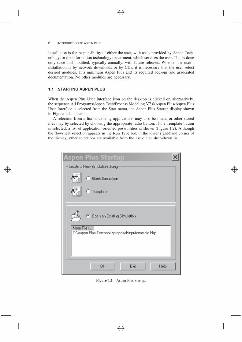
When the Aspen Plus User Interface icon on the desktop is clicked or, alternatively,the sequence All Programs/Aspen Tech/Process Modeling V7.0/Aspen Plus/Aspen PlusUser Interface is selected from the Start menu, the Aspen Plus Startup display shownin Figure 1.1 appears.

A selection from a list of existing applications may also be made, or other storedfiles may by selected by choosing the appropriate radio button. If the Template buttonis selected, a list of application-oriented possibilities is shown (Figure 1.2). Althoughthe flowsheet selection appears in the Run Type box in the lower right-hand corner ofthe display, other selections are available from the associated drop-down list.

Figure 1.1 Aspen Plus startup.

GRAPHIC USERS INTERFACE 3

Figure 1.2 Preconfigured selections.

If the option “blank simulation” is chosen, an application can be custom configured.After selecting the desired option and clicking OK, the Connect to Engine screenappears, and upon selecting OK, a blank workplace that facilitates the graphic usersinterface appears if “flowsheet” was chosen. If the option chosen is anything else, thefirst required input form appears.

1.2 GRAPHIC USERS INTERFACE

The graphic users interface (GUI) is the means by which a flowsheet is defined. Theprocess consists of placing blocks and streams on the workplace and connecting them.Aspen Plus assigns generic names such as B1 to the blocks. The user may change thesenames by right-clicking on the element of interest and using the menu that appears.Blocks are selected by choosing a category tab from the model library—for example,Mixers/Splitters—and clicking on the icon that represents the block desired. Afterclicking, a movable + sign appears on the open area of the display. After positioningit on the screen, a left click will place the block. The + sign remains and can bemoved to insert another instance of the same block. This function ceases when thearrow button at the lower left is selected. In identical fashion, streams can be placedon the flowsheet. Material, heat, and work streams may be selected. When a streaminput is selected and the cursor is moved onto the workplace, the ports to which thestreams may be connected are shown. The connection is made by moving the active


Figure 1.3 Connecting streams.

cursor over an open port and clicking. An example of connecting streams to ports isshown in Figure 1.3.

All icons, block names, and stream names can be selected and moved using standardWindows techniques. Similarly, streams can be moved, rerouted, disconnected, andreconnected. Selecting and right-clicking on any of the objects displays a menu thatprovides many useful functions for manipulating the graphics. These include changingicons, rotating objects, renaming, deleting, and aligning the graphics.

1.3 NEXT BUTTON

Aspen Plus provides the user with a mechanism for filling out forms in an orderlyfashion. At any point after the flowsheet has been fully defined with the GUI, theuser may select the Next button, which appears as the symbol N → on all forms.The Next button moves to the next form required. On occasion, after using the Nextbutton, Aspen Plus will prompt the user to select from a choice of actions to be taken.The Next button provides only the minimum required input. As an example, when anactivity coefficient equation to be used in the simulation is chosen, Aspen Plus will use

SETUP SPECIFICATIONS DISPLAY 5

a default data source, such as a vapor–liquid equilibrium (VLE) source; however, ifthe simulation involves liquid–liquid equilibrium (LLE), it is the users’ responsibilityto select the appropriate data source. Aspen Plus will not open the appropriate displaysby using the Next button.

1.4 SETUP SPECIFICATIONS DISPLAY

After the flowsheet has been defined with the GUI, pushing the Next button bringsup the Setup Specifications—Data Browser display. The Data Browser panel of thedisplay should show a list of all possible categories that can be chosen for selectingvarious options and for entering appropriate data. If the setup information shown inthe left panel of the display does not appear, choosing the upper menu selection, Data,and entry Setup will present the Data Browser panel, shown in Figure 1.4. If the listof process model icons shown at the bottom of Figure 1.4 does not appear, clickingthe View menu Model Library will display them.

When starting a problem, the Setup Specification display provides a drop-down listassociated with the entry box Run type, which shows the six primary functions thatAspen Plus is capable of:

Figure 1.4 Setup specifications for data browser.


1. Data regression: fitting data to models

2. Flowsheet: process simulation

3. Property display: showing properties of a component in Aspen Plus’s database

4. Property analysis: estimating physical and thermodynamic properties

5. Assay data analysis

6. Property plus

The last two functions are not considered here. The user selects the required functionto initiate data input for a specific requirement.

Note that the Data Browser panel shows a blue check next to various items. Thisindicates that the default values are sufficient to proceed with data input; however, thisis the minimum data required and the values may be modified to meet the requirementsfor any problem. The red elements on the browser panel list indicate that user inputis required. A red element may be deleted by right-clicking on it and selecting Deletefrom the menu that appears, or if Aspen Plus permits, and sometimes by using theWindows delete key.

There are drop-down lists for all the categories in the data-entry boxes under theGlobal tab, and all may be changed. For example, the value Mole has been selected forthe option Flow basis. Additionally, under units of measurement, the input and outputunits have engineering (ENG) as default values, while the associated drop-down listoffers Metric and SI units as other possibilities.

Aspen Plus provides a Help button, on the topmost menu, for accessing informationby subject. Additionally, help with any entry on any display is available by movingthe cursor to the entry and pushing F1 or selecting the ↖? button on the tool bar.

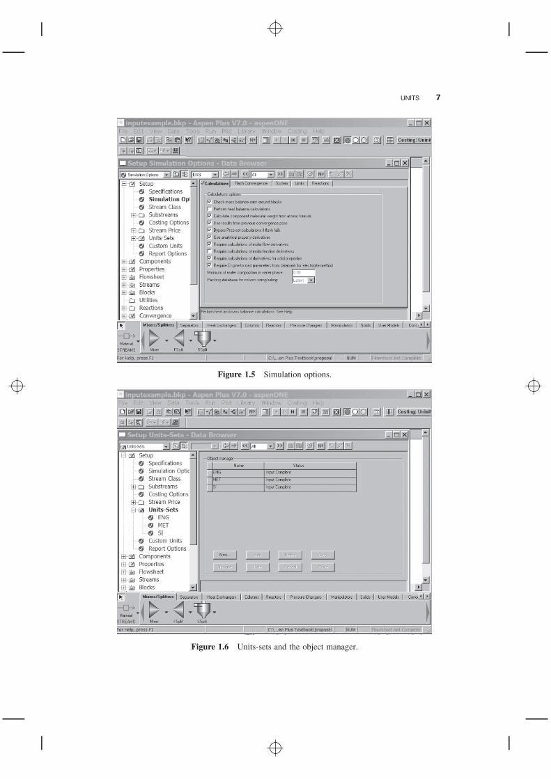
1.5 SIMULATION OPTIONS

If the Simulation Options category is selected, the Simulation Options display shownin Figure 1.5 appears. All of the default values that appear under the various tabs neednot be changed except under the tab Calculations, where the option not to use energybalances in the calculations is available. This is an important option for preliminarycalculations. If simulations do not involve solids or electrolytes, the appropriate optionsmay be unchecked.

1.6 UNITS

Aspen Plus provides a user with a choice of units: engineering, metric, and the inter-national system of units, SI. An important option is the ability to select mixed units;for example, the choice of engineering units with mmHg and degrees C as temperatureand pressure is not uncommon in some pharmaceutical applications. To accomplishthis, Units-Sets is selected from the Data Browser menu, which produces the ObjectManager shown in Figure 1.6. Then, selecting New produces an Identifier for the newunit set, in this case US-1, and a choice as to whether or not to assign this as a globaldata set. Then Figure 1.7 appears.

UNITS 7

Figure 1.5 Simulation options.

Figure 1.6 Units-sets and the object manager.


Figure 1.7 New units.

The Copy from entry permits selection of which unit set to use as a base. Note theselection of degrees C from the temperature drop-down list. Each unit’s entry has anappropriate drop-down list, which will enable a user to customize units.

Custom units for a specific variable—for example, special composition units—maybe defined by selecting the Custom Units entry under the Setup list.

Aspen Plus input forms, displays, and reports are generated using the units selected.Input displays typically have a drop-down list adjacent to input boxes which permitsthe user to select the units of the input data required. This does not, however, affectthe units used for output.

Selection of the Report Options entry under the Setup list permits customization ofthe Aspen Plus results displays and the. txt report, which can optionally be generatedwhen results are available. Details are given in Section 1.11.

1.7 COMPONENTS

Selecting the Components item on the Data Browser panel produces Figure 1.8. Com-ponents may be entered by either component name or chemical formula. Aspen Plusalso requires that a nickname, Component ID, which is used in all stream reports, beprovided for all components.

COMPONENTS 9

Figure 1.8 Component selection.

An entry in the box Component ID is a user-provided component short nameemployed by Aspen Plus for report purposes and in some cases, such as water, isrecognized as the component water. An entry is always required. Alternatively, theuser may enter a proper component name or component formula. If neither is rec-ognized as an entry in the database, the user may select the Find button and AspenPlus will display a set of names or formulas that incorporate the entry. For example,entering the formula C7H8 gives the results shown in Figure 1.9. Upon selection ofthe component of interest, pressing the Add selected compounds button enters thecomponent into the data associated with the current Aspen Plus run.

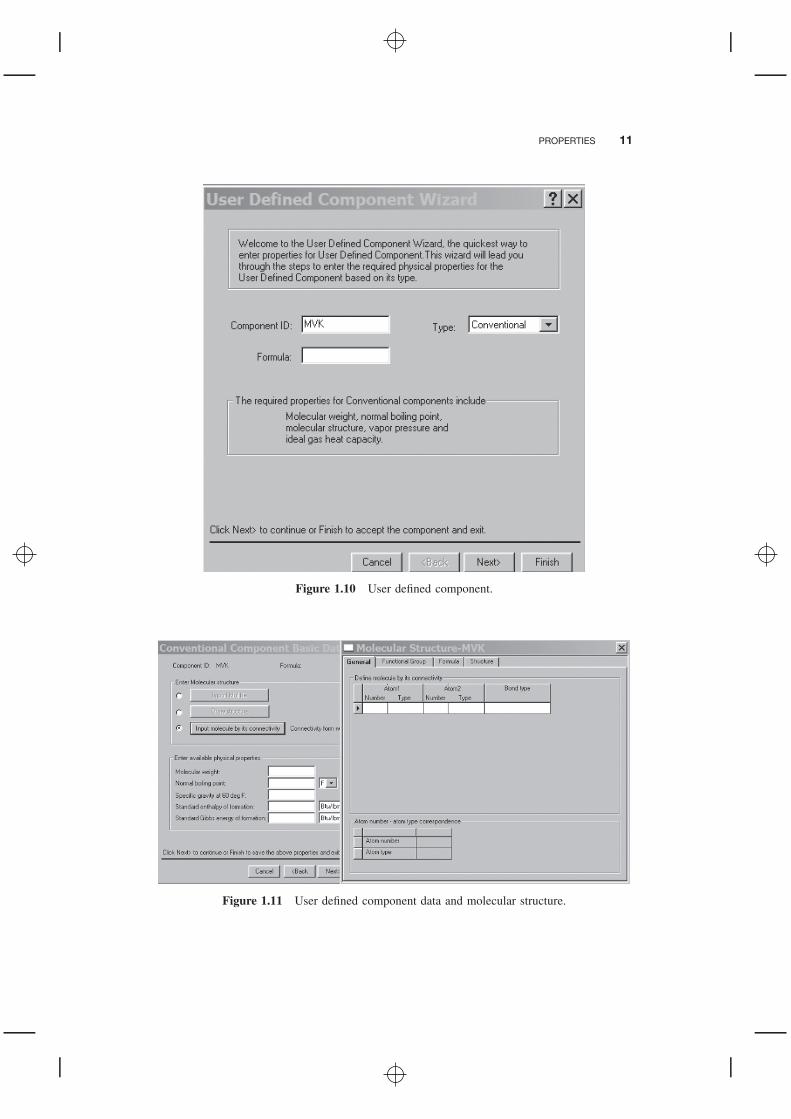
If a component does not exist in the Aspen Plus database, choosing User Definedin Figure 1.8 produces the User Defined Component Wizard shown in Figure 1.10.

Note that several properties are required. After entering the Component ID andformula, the Basic Data and Molecular Structure displays shown in Figure 1.11 appear.Known experimental data and structural information are entered. As the data-entryprocess proceeds, an option for Aspen Plus to estimate any missing data appears.Chapter Two concerns methods for estimating data which may be employed selectivelyfor supplying the missing data above rather than permiting Aspen Plus to providemissing data using default methods.


Figure 1.9 Component search.

1.8 PROPERTIES

The first display when selecting properties for a simulation is given in Figure 1.12,where the choice of a global property method that applies to an entire flowsheet maybe selected. If, however, the simulation involves a situation where more than prop-erty method is required, for example, a process involving distillation (vapor–liquidequilibrium) and extraction (liquid–liquid equilibrium), each block in the flowsheet isidentified as part of a unique flowsheet section when the flowsheet is created, and isidentified with a particular property method by choosing the Flowsheet Sections tab.A display similar to Figure 1.12 appears; the properties method for each flowsheetsection can be identified and a global property method is not used. The Tools menucontains the Property Method Selection Assistant, which can be used as a guide forselection of a property method for specific applications; alternatively, the small boxto the left of the Uniquac selection in this example, although not explicitly labeled,performs the same function.

For this example process, sections S-1 and S-2 are assigned the property methodsUniquac and Uniq-2. Aspen Plus sets up the required Uniquac binary parameters foreach selection. Care must be taken that the appropriate database is accessed for each set

PROPERTIES 11

Figure 1.10 User defined component.

Figure 1.11 User defined component data and molecular structure.


Figure 1.12 Global property method.

of parameters. As an example, if the Data Browser topic Properties/Parameters/BinaryParameters is selected and the listing Uniq-1 is clicked, Figure 1.13 appears. This showsthe values of Aspen Plus–supplied parameters for each binary pair and the source ofthe data used in the regression. In Figure 1.13, note that the source of equilibriumdata for each binary pair is identified. A selection of data sources is available bychoosing the tab Databanks, which produces Figure 1.14. In the current example,section S-1 contains the extractor, and it is therefore important that the data source beliquid–liquid equilibrium data. Section S-2 involves a distillation column; hence thebinary parameters source is vapor–liquid equilibrium data.

1.9 STREAMS

Pushing the Next button moves the input sequence to stream data. All feed streamsare defined using a display such as that given in Figure 1.15. The data entry is verystraightforward and provides a user with the possibility of changing the units of boththe material flow and the state variables. For a stream of a single component or severalcomponents, the number of degrees of freedom calculated by the Gibbs phase ruleapplies:

F = C − P + 2

STREAMS 13

Figure 1.13 UNIQ-1 parameters from Aspen Plus databank.

Figure 1.14 Available databanks.


where F is the degrees of freedom, C the number of components, and P the num-ber of phases. For a single-phase system, F = 2; therefore, two specifications arerequired. For an n-component system, F = n + 1. Since n − 1 mole fractions needto be specified and the last calculated by the sum of the mole fractions equal to 1,only two additional specifications are required. In both cases these are usually, but notnecessarily, temperature and pressure.

When two phases in equilibrium are involved, only one degree of freedom is avail-able. For example, for a one-component stream such as a saturated liquid, specificationof the temperature fixes the (vapor) pressure. But in such circumstances it is neces-sary to state the fraction of the mixed stream that is vapor (or liquid). For a saturatedliquid the V/F specification would be a very small number, such as 0.00001. For amulticomponent stream the situation is identical and it is necessary to specify eithertemperature or pressure and the vapor or liquid fraction.

If the process contains tear (recycle) streams, they will not be treated as requiredinput, and pushing the Next button may not suffice. Typically, Aspen Plus will assignzeros as starting values to the variables that are to be converged, but if a user wishesto provide starting values, the stream name under the streams list in the Data Browsercan be clicked and a display analogous to Figure 1.15 will appear.

1.10 BLOCKS

When all stream input has been completed, pushing the Next button will result inthe appearance of the first input form for a block that requires data. Details of blockinput are addressed in other chapters. After the data input forms for the first block arecompleted, pushing the Next button will produce the forms for the next block in theprocess until all the block data have been entered.

The browser list in Figure 1.15 shows some additional topics that may be appropriatefor a user’s simulation. These will not appear when the Next button is pushed; however,they may be selected by clicking on the subject. For example, clicking the Convergenceentry permits the selection of the convergence method and parametric default values.These subjects are addressed in other chapters. When data entry for all blocks andsupplementary data entry is completed, selecting the Next button produces a dialogueto enable execution. All input can be reviewed, prior or after execution, by selectingthe � or � keys above the Flash Options tab near the top of Figure 1.15 and selectinginput from the drop-down list between the double arrows.

1.11 VIEWING RESULTS

In preparation for viewing the results, prior to execution of a simulation, a user maycustomize reports by selecting Report Options, as shown in Figure 1.16. Customizationis available under each of the tabs. The stream tab illustrates the variety of optionsavailable for selecting the stream information to be displayed.

At the conclusion of a simulation, the run control panel is usually displayed. Ifnot, it can be viewed from the drop-down list under the main menu item View. Thiscontains a brief summary of the execution of each block and a list of error messages. Itis important that users check and correct any errors that might have occurred. When aprocess contains tear streams, errors that occur during the iterations will be presented.

VIEWING RESULTS 15

Figure 1.15 Stream specifications.

Figure 1.16 Report options.


Figure 1.17 Run control panel.

It is not uncommon that errors occur before convergence, but when the process hasconverged, there should be none. Figure 1.17 displays an example of the run controlpanel. The results of the simulation can be viewed by selecting the Results button,which contains a check symbol overlaid on a file symbol on the fourth row from thetop of the display.

Selection of the Results button produces a display similar to Figure 1.15, with thecentral drop-down list displaying results. Selection of the � or � keys permits pagingthrough all the results. If All is selected from the drop-down list, one may view bothinput and results in order.

When a simulation has been completed, selection of Report from the main menuitem View will produce a. txt report of the complete simulation, in a Notepad windowthat can be copied and pasted.

The file Chapter One Examples/inputexample.bkp was used to produce all of thefigures in this chapter as well as the inputexample.txt file.

1.12 OBJECT MANAGER

In certain data input situations there are specialized setups that involve the specificationof material that requires a special set of dialogues to define what is required. Examples

PLOTTING RESULTS 17

Figure 1.18 Object manager.

are: definition of a set of properties to be displayed, regression of a data set to athermodynamic model, and specification of the value of a block output variable. Thistype of input is managed through use of the Object Manager. These situations typicallybegin with the identification of a function, such as a regression, followed by a seriesof choices and specifications. An example of the use of the Object Manager for aCalculator block, which is used for in-line calculations, is given in Figure 1.18. Theuser creates an ID such as C-1, which is followed by all the input forms required,including association of calculation variables to flowsheet variables and definition, inFortran, of the calculation details.

1.13 PLOTTING RESULTS

Aspen Plus has a plotting facility accessed through the Plot menu. The facility eitherprovides the selection of independent and dependent variables manually or by meansof a Plot Wizard, which permits the user to select a preconfigured plot. As an example,after obtaining a converged solution to a distillation column, selecting the Plot Wiz-ard, and pushing the Next button, a collection of distillation-oriented plots, shown inFigure 1.19 is available. Selecting the Comp plot produces Figure 1.20, which showsthe change in vapor composition through the column. For situations where preconfig-ured plots are not available but a display of tabular output is available, such as theresults of a sensitivity analysis (details in Chapter Five), one may select a column ofdata and assign it to either the x or y coordinate. It is also possible to assign two vari-ables to the y coordinate by holding down the control key when selecting the columnsof data that are to be employed. If the scale or title of an axis or title of a plot is


Figure 1.19 Plot wizard.

Figure 1.20 Sample plot.

REFERENCES 19

not suitable, one may select it by clicking, and a display that offers editing optionsappears.

REFERENCES

Aspen Plus version 7.0 documentation.Monsanto Corporation, Flowtran Simulation: An Introduction, 1974.

introduction to aspen plus - beck-shop.de · pdf file2 introduction to aspen plus installation...

Documents