iGETT Tutorial

Introduction to ArcGIS 10

Focused on

Natural Hazards: Landslides and Wild Fires

Student Handout

Ann Johnson Co-Director, iGETT Project

Associate Director, GeoTech Center gisajohnson@delmar.edu

2

iGETT Tutorial

Introduction to ArcGIS 10 Focused on Natural Hazards:

Landslides and Wild Fires

Including Other Topics Useful in Environmental and Earth Science

Introduction and Background Information

This project focuses on a study area in San Bernardino County, California, which includes

numerous landslides, faults, and changes in elevation. It is also an area that has been affected by wildfires and rain induced mudflows. This exercise will focus on areas that experienced wildfires in October 2003 and that may be more prone to landslides. Tragedy struck on December 25, 2003, when 8 inches of rain fell in Waterman and Cable Canyons in a few hours causing mudflows and flash floods killing 16 people.

This exercise uses real-world data to help identify areas that may have higher landside susceptibility and includes such factors as slope, aspect, vegetation and burn severity. You will need access to ArcGIS 10 and Microsoft Excel. To complete Part V you will need access and the ability to download large Landsat imagery from the Internet.

The project is divided into five parts, with each part introducing new and more advanced processes or techniques for displaying and analyzing data. Part I introduces ArcCatalog and geodatabase data structures and includes an introduction to many basic operations, data types and visualization techniques; Part II introduces geoprocessing and analysis of data using various tools and introduces ArcGIS 10 Extensions. Part III introduces Model Builder and Creating a Model to automate analysis. Part IV briefly looks at animating data analysis in 3D. Part V uses the new tools that can be used to do basic remote sensing analysis.

In this project you will use Digital Elevation Data (DEM) to derive slope and aspect datasets and fire data to suggest areas that have a higher susceptibility to landslide. The values and models for determining landside susceptibility are for educational use only and should not be used to determine slide hazards or areas safe from landslides, as there are many factors that are not considered in this exercise.

3

Part I – Student Handout

Introduction to ArcGIS 10ArcMap and ArcCatalog

Natural Hazards: Landslides and Wild Fires in San Bernardino, CA

Part I of this Tutorial will introduce ArcMap and the Dockable Catalog window. It will also introduce basic data access, creation and display. It includes steps to understand the data structure, bring in field (GPS) data, create new data, visually analyze data and share data with other people who do not have access to ArcGIS. ArcCatalog 10 is now imbedded in ArcMap as a dockable window. It is also a separate application that provides access to your geospatial data. While it looks a lot like Windows Explorer, it is much more functional in regard to ArcMap projects and geospatial data access, creation and structure. Step 1: To become more familiar with the file structure and the data used in this project we will begin by opening ArcCatalog and looking at datasets and data structure for the project.

q Double click on the icon for ArcCatalog (or click Start > Programs > ArcGIS > ArcCatalog 10).

q Make a direct connect to SB_CA_Geo project by clicking on the Connect to Folder button and using the dialog box browse to the drive where your ArcProjects folder is stored, then click on name of folder SB_CA_Geo. Click OK

q It should look similar to:

You now have a direct link to C:\ArcProject\SB_CA_Geo when you open ArcCatalog. Step 2: Take a look at the Data Structure for the SB_CA_Geo project. Note: When opening raster datasets you may be prompted to create pyramids – click “Yes” if this prompt is displayed.

q Click on the + to expand the folders in the “Catalog Tree” portion of the application.

q Expand the subfolders (click on + by each subfolder) and look at the names of the files under each subfolder. Right click on one dataset and go to properties and review its properties. Right click on the sb_dem grid data set. Click on the minus – by any folder if you want to close it.

4

q Expand the “LYR_Files” subfolder and the SanBern.gdb (click on +) Local11N27. Note that each feature dataset in the Geodatabase SanBern.gdb has the same Coordinate System and Projection which is noted by its name – LocalN11N27 (local data in UTN 11 North, NAD 1927). Note too that “Layers” do NOT contain data, but are instructions that ArcGIS uses to symbolize the data that is contained the SanBern.gbd Also note the different colors for the layers versus data sets and how the symbol icon next to the name represent points, lines or polygons.

• Right-click on one layer, go to Properties and review • Compare the difference between layer and feature class or

other object properties. Note too that the name of the Layer does not always match exactly the data it represents.

q Click the sb_dem.lyr and then Click on the “Preview Tab” and

select “Geography” in the Preview window. This is elevation data with lower elevation pixels darkest gray to black and highest elevations as white. Click on a couple of other .lyr layers and preview the Geography. Note: When opening Grid datasets you may be prompted to create pyramids – click “Yes” if this prompt is displayed.

q Click the + for LocalU11N27 to expand it and select SB_burn_severity (a polygon feature class).

Pick the Preview Tab and change to “Table”. Note in the table that there are three attribute classes in the VEGBURSEV column (Low, Moderate and High). We will be using this attribute data in our analysis.

q Right Click on the grid file named sb_dem in the San_Bern.gdb and pick Properties. This will open a window that shows details related to this data set such as Cell size and vertical units and Spatial Reference. Click OK to close the Properties

q Collapse all of the folders at once by clicking on the “–“ by any expanded folder while holding

down the CTL key. You can also Open all folders using the Ctrl key.

q Close ArcCatalog application. Step 3: Now that you have seen what data is available, we are ready to open ArcMap and begin investigating the use of ArcGIS 10 for geologic analysis of the region for natural hazards. Collecting field data is integral to natural hazards and geological studies. A GPS can be used to collect location data with attributes about the location. For this study a short field trip was made to the Waterman Canyon area and a GPS was used to collect Latitude and Longitude locations and a digital camera was used to record photos for each location. An ArcGIS project was created for the San Bernardino study area, and the photos where then hyperlinked to the location in the study area. We will continue working on the study area to create two new locations using Excel. We will then use the Editor tools to create a new possible fault in our study area.

q Double-click on Icon for ArcMap or Start > Programs >ArcGIS > ArcMap. q Click on “Existing Maps” then “Browse for More” and

Browse to C:\ArcProjects\SB_CA_Geo\ and click on SB_Geology_V1.mxd and click Open.

q Use the Zoom in Tool to zoom into the region where the point symbols for the Photos are located on the map. (Click on Zoom in Tool and click and drag a box around those symbols – repeat until you can see the individual symbols).

5

Alternatively, you could right-click on the Photo_loc layer in the Table of Contents and choose Zoom to Layer. This will zoom to show all the photo locations.

We may want to return to this map extent so we are going to create a Bookmark that we will use t o return to this region.

q Click on Bookmarks and click Create. Name the Bookmark “Photo Extent” and click OK. . q Now click on icon for Zoom to Full extent and then return to the Photo Extent by

using the Bookmark in the Bookmarks menu. The dark brown polygons are previously mapped landslides and are part of the SB_Lndsld dataset. You may want to go to different regions of the study area so you will create 5 more Bookmarks.

q Zoom in and out to full extent and locate other areas of the map (northeast, southwest, etc.) and

create 4 more bookmarks with appropriate names. Create an additional Bookmark so that the entire region of the study area covers the Map area. Name this Bookmark Study Area.

q Click on Bookmarks > Manage and reorder them using the up and down arrows so they are in a better order. If you don’t like a bookmark, you can remove it using Manage. Click Close when you are finished with reordering bookmarks.

q It is important to know what happens when you click on the + or left click or right click on the name of the dataset or it symbol. If you click on the + by the Geology Polygons it expands and you can see the Legend for the features in the dataset. If you click on the square it draws the dataset in ArcMap. If you click and uncheck it, it is not drawn. Clicking on the symbols (left or right) you can change the color or the size of the feature. Using the above information, expand and click on different datasets or data in the legends to investigate what happens when you click on different parts of a dataset layer in the Table of Contents.

Step 4: Next we are going to look at some photos that are linked to the locations for the Photo_loc points feature dataset using the Hyperlink tool.

q Click on the Hyperlink tool and note that the Photo_loc points now have a blue center. Note:

use the Bookmark you created to zoom in to the location if necessary. q Click on one of the blue dots with the tool. A photo should open for that location. (HINT: If you

have problems getting the hyperlink tool to bring up the photo, go to the menu Selection > Options and change the selection tolerance to 5 and click OK).

q Close the photo (click on X in upper right corner) and click on another location that is hyperlinked.

q We can also Label these locations on the map, but first we will pick what attribute field will be

used as a label. Double click exactly on Photo_loc name in the Table of Contents and select Labels tab. Check the box “Label features in this layer” and in the Label Field box select Photo_Desc. Click OK.

q SAVE your project.

q Optional: Please note: These Hyperlinks are hard coded to C drive in the Hyperlink attribute field. If this is not the drive you are using to store the data, you will need to Edit the table to change to the correct Drive. To do this, Right Click on the Pholo_loc layer name and Open Attribute Table. Add the Editor toolbar (Customize > Toolbar > and check on Editor then on the Editor toolbar click Start Editing. In the table scroll the Hyperlink Attribute field and change each “C” to the correct Drive letter for each photo. Then click Editor > Stop Editing – if prompted, click Yes to save edits.

6

Step 5: It is often necessary to create new feature data sets from data collected in the field. The data can be collected using various methods, but here we have used a GPS unit to determine the Latitude and Longitude of two features that we want to note in our study. We are going to use Excel to show how a dataset can be created using a spreadsheet. If you do not have access to Excel, you can also use other methods for creating point dataset (see Help for other options). After we create the dataset, we will hyperlink a satellite image taken during the 2003 fire provided by Digital Globe to one of the new features.

q Open Excel (Go to Start > Programs > Microsoft Office > Excel). We have Latitude, Longitude and Attribute data for two locations in the study area. One is by a road intersection and one is by a fault contact. Remember when creating an Excel spreadsheet, you must use the first row for the “header” fields. We will use LAT, LONG and ATTRIBUTE as the three headers (no spaces, use only alpha/numeric characters and no more that 13 Characters) for 3 Columns in the spreadsheet. Note: A data dictionary that describes each data set should be created as a separate document. You can also create alias names for column headers (see Help for more information). In the Excel spread sheet create a spreadsheet with 3 Headers and the data EXACTLY shown below:

q Save the Excel Spreadsheet in the C:\ArcProject\SB_CA_Geo\Table folder with the name of Test_Data and close Excel. Return to ArcMap and use File menu > Add Data and click on Add XY Data. Where you see “Choose a table from the map or browse for another table”, browse to your saved Excel spreadsheet, double-click on the name Test_Data, and select Sheet1$ then click Add.

a. Important Note: ArcGIS automatically set the Coordinate System to the one used in

the Geodatabase for this project. This Test_Data dataset is not projected, it uses Latitude and Longitude and is in Geographic. You MUST Edit the Input Coordinates by clicking on Edit. The data was collected on a GPS using NAD 27 Datum, so select Geographic Coordinate Systems and then click on North America and select NAD 19927.prj and Add. Then click OK.

q You will receive a warning; read the details as we will use these steps to create a new

feature class, then click OK. Note that since spatial reference is defined here and for the map data frame, ArcMap will “on-the-fly” project all data to properly align. You can zoom to the layer by right clicking on Sheet1$ Events and “Zoom to Layer”.

q You will now create a point feature class from this XY data so that you can use it more fully. Right

click on the Sheet1$ Events data and select Data > Export Data. In the Export Data dialog window click on the button that says “the feature dataset you export the data into.” For Output feature Class use the Browse folder button and browse to C:\SB_CA_Geo \Geodatabase\SanBern.gdb\LocalU11N27 and highlight the default name and re-name in Name it Test_Data. Click Save and OK then click Yes to add to map layer if asked. Right click on the Sheet$ Events layer and select Remove.

q Note: ArcGIS will usually provide a “default” name to new datasets. If you do not want to use the

default, you must highlight the default name and re-name it. It may be necessary to “scroll” over to see the default name in the Output raster name in order to highlight it.

7

q Zoom back to the full extent of the study area by clicking on the Full Extent tool. Use the Zoom In tool to zoom to new data set region and create a Bookmark called Test Data. You can click on the symbol in the Table of Contents and in the dialog box that opens, increase the size of the symbol and change its color. Close the dialog box.

q Click on the Identify tool

q Click on one of the features in the Test_Data (either the road or fault) in the middle of the study area.

q Right-click on the “name” (road or fault) of the feature in the “Identify Results” dialog box and

click on Add Hyperlink.

q Browse to C:\ArcProjects\SB_CA_Geo\Images\RS_Image and click on fire-unref.jpg and click Open. (Note: you may have to turn off any “popup blockers” to allow images to open.)

q Click OK in Add Hyperlink window.

q Close the Identify Results dialog box and click on the Hyperlink tool.

You will see that the feature you picked above to hyperlink to has a blue center.

q Using the Hyperlink tool, click on that feature and the image will open. You can zoom in on the image and see the region covered by the study area.

q You may have to select the pointer tool to stop the hyperlink tool.

q Right Click on the Test Data name and select Save as a Layer File in the LYR_Files folder that is in the Geodatabase folder in your SB_CA project and leave name as Test_Data and click Save. Note: Each of the Layer Files for all of the feature datasets were created in the same way. Note: Layer files say how data is symbolized, but the data remains in the database.

Step 6: Part of the field work has suggested that there may be other unidentified faults in the study area. We are now going to draw a fault up the central trace of Waterman Canyon. You can locate Waterman Canyon by turning on the sb_drg_clp dataset and turning off other layers. Waterman Canyon is located to the east of the Photo locations or if you are connected to the Internet, you can add data from ArcGIS Online by using the File menu, ArcGIS Online and searching on Topo Maps. Select USA Topo Maps and click on Add. Use your Photo Extent Bookmark and locate Waterman Canyon to the east of the photos.

q Turn off all datasets (uncheck boxes by their names one at a time or hold Ctrl key and click on any one) except the Photo_loc, HillShade and Faults, and use your Bookmarks for Photo Extent to Zoom in to an area that clearly shows this canyon. Turn on the sb_drg_clip and turn off Hillshade to double check location. The sb_drg_clip is a portion of a digital raster graphic covering the study area.

8

q Recheck the sb_dem and Hillshade. Then add the Editor toolbar if you have not done so by using the Customize menu > Toolbars and check on Editor toolbar.

q Using down arrow in the Editor toolbar click Start Editing. A new Create Feature dialog box

opens with the Faults listed in from the Table of Content. This new fault is possibly a Right Lateral Strike Slip Fault so highlight the first one of that type in the Create Features dialog box.

q The Construction Tool shows that a line feature class tool is available and the mouse is now a drawing tool. Click and drag and click along Waterman Canyon drawing a new fault, double clicking at last location. It turns blue. Click Save Edits and Stop Editing on the Editor Toolbar. You now have a new fault.

Step: 7: Now that you have identified a possible new fault, you may want to field check it or have others that do not have access to ArcGIS field check it. You can create a PDF of your project and share it.

q First Save your project (File > Save As) and name it SB_Geology in SB_CA_Geo. Then turn on all layers and Zoom in to an area of interest that clearly shows your new fault. You may want to change the symbols for some of your data sets. Once you are happy with your map, Save again.

q Click File menu > Export Map and change File name to New Fault Map in Waterman Canyon, and select PDF for the file type. Browse to Miscellaneous folder for your project and then click SAVE

q You can now use Microsoft Windows Explorer and browse to Miscellaneous folder and open the PDF. Click on the Layer Stack and click on an “eye” to draw or not draw a layer. You can now send this to other people and have them turn on and off layers.

Waterman Canyon

9

We now want to see if there is any correlation between mapped slides, the rock type (geology) and the proximity to the San Andreas and other faults in the study area.

q First Save your project (File > Save) as SB_Geology.

q Be sure to have the Geology Polygons, Faults and Landslides datasets drawn and legends visible (click on + by dataset name and a check in the box next to the name) to see the symbology for these two data sets. Turn off unneeded layers.

q Now use the Zoom In and Zoom Out and Identify tools (click as needed) or use the Bookmarks

you created to look at the type of rock that the different Landslides occur within. Note: you will need to make the Geology Polygon layer the target layer for the identify tool, then click on various polygons and scroll to the Field named UNIT NAME or SUMMARY1 to see what the rock type is (i.e., igneous, metamorphic, sedimentary, alluvium, etc.). We have created a “Layer” out of the geology dataset so that the different types of rock have unique symbols. A “layer” .Lyr points to (uses) the data in the geodatabase, but retains the specific symbols that have been used for the attributes of the features. The major divisions in the geology dataset are Igneous, Metamorphic and Sedimentary with several different types of Alluvium. There is also a Landslide dataset of mapped landslides.

q Are all the Landslides in one rock type (igneous, metamorphic, sedimentary) or do they appear to be in different types? Are they all near fault lines?

Your visual inspection should suggest to you that slides can occur in different types of rock formations and near or further away from faults. So we can visually conclude that rock type or fault proximity are not useful indicators to suggest where landslides may occur. Step 8: We will now visually investigate the slope of the study area by creating Profiles across a few locations in the study area using the 3D Analyst Toolbar. This will help us understand how the slope changes from the valley floor, across faults and into the higher regions of the San Bernardino mountains. Before doing that, we will create a Contours Dataset so that we will have additional information about the changes in elevation.

q Using sb_dem layer we will determine the range of elevation in the study area. Right click on sb_dem and select Properties > Symbology tab. The Statistics for Band_1 show a minimum of 335..3 (approximately) and 1968.3 maximum. Since this is in meters, the lowest elevation is above 300 meters and the highest is below 2,000 meters. (Note the units in the sb_drg_clip are in feet). We will use that range for our contours with in interval of 30 meters. Close the dataset Properties.

q First be sure to turn on the 3D Analyst extension (Customize menu > Extension > 3D Analyst is checked) and add 3D Toolbar (Customize > Toolbar > 3D Analyst) is checked.

q You can create contour lines from the sb_dem data using a Tool from the ArcToolbox. To find

the tool, use the dockable window for Search (use mouse and hover over the Search dockable window and click). Type “Contour” into the search window and enter. Click on the Contour 3D Analyst tool name. In the Contour window for input raster use the sb_dem. For output, browse to the San_Bern.gdb, LocalU11N27 and name it Contours30. For interval choose 30. For base use 300. Click OK. You will see the tool being run by the blue letters in the lower right of the project window. Once it is completed successfully, the Contours will be added.

We are now going to look at the topography of the area.

10

q Turn off all datasets except Contours and Hillshade to better view the topography (relief) – use your Bookmark to zoom to Photo Extent to see the contours. Then use bookmark and go to Study Area.

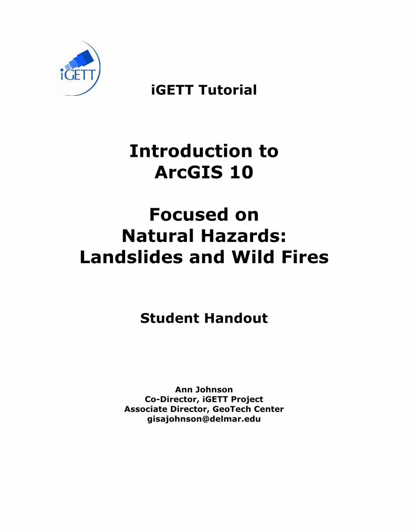
q Set the “Layer” on the 3D Analyst toolbar to sb_dem. Click on the Interpolate Line tool. Then on the map, click and drag a line across the study area from the valley to the mountains (double click where you want it to end). On the 3D Analyst toobar click on the Create Profile tool that becomes active after creating the line (note, you may have to use the down arrow on the create point tool to see it. A profile will be shown that corresponds to the line you have just drawn.

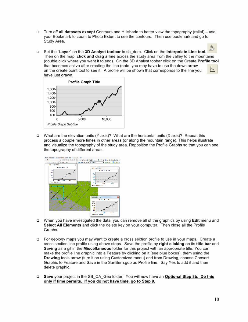
q What are the elevation units (Y axis)? What are the horizontal units (X axis)? Repeat this process a couple more times in other areas (or along the mountain range). This helps illustrate and visualize the topography of the study area. Reposition the Profile Graphs so that you can see the topography of different areas.

q When you have investigated the data, you can remove all of the graphics by using Edit menu and

Select All Elements and click the delete key on your computer. Then close all the Profile Graphs.

q For geology maps you may want to create a cross section profile to use in your maps. Create a

cross section line profile using above steps. Save the profile by right clicking on its title bar and Saving as a gif in the Miscellaneous folder for this project with an appropriate title. You can make the profile line graphic into a Feature by clicking on it (see blue boxes), them using the Drawing tools arrow (turn it on using Customized menu) and from Drawing, choose Convert Graphic to Feature and Save in the SanBern.gdb as Profile line. Say Yes to add it and then delete graphic.

q Save your project in the SB_CA_Geo folder. You will now have an Optional Step 8b. Do this

only if time permits. If you do not have time, go to Step 9.

Profile Graph Title

Profile Graph Subtitle10,0005,0000

1,6001,4001,2001,000800600400

11

Step 8b: Optional – Please go to Step 9 unless you have a lot of time and a great deal of patience: Georeferencing an image to your project. The process is an important one. That is, using a georeferenced vector data set to georeference a raster dataset. You can read through the steps and not actually carry them out to learn the process. This is an Optional Step as it takes a great deal of patience and time to bring this particular image (which is not high resolution and is obscured by smoke) into a position (georeferenced) that closely aligns with the vector and other raster data. If you do not have time to do this, just read the steps and skip to Step 9. The sb_drg_clp layer and the Test_Data (point at road and fault) may help you to orient yourself and check your results. Before beginning, open the fire-unref.jpg in Windows Explorer and note locations of major freeways and the catch basins at the base of Waterman Canyon as well as the Canyon and stream locations. Be sure to make your first location as precisely as possible. The second location should be a distance from the first one and in a location that you can see through the smoke. If you make an error, remove the reference points by using the table that is part of the Georeferencing toolbar. Remember too that you need both the image and at least one vector data set that is in the projection and coordinate system to which you want your image to be aligned (georeferenced).

q First add the Georeferencing toolbar (use menu Customize >Toolbars, Georeferencing) and position it where you find convenient. Turn off all layers except the Roads layer.

q Add (using + button) the fire-unref.jpg image from the Image folder, RS_Image. It may ask to

build pyramids, click yes and tell you the image is unprojected which is correct. Zoom in by right clicking on the fire-unref.jpg name > Properties > Zoom to Layer and locate those areas with roads leading into the Waterman Canyon area and just south of that area. Look for those locations you noted using Windows Explorer including roads you can see as cross roads to use in Georeferencing. Zoom back to full extent.

q On Georeferencing toolbar select the fire-unref.jpg as the Layer and then go to the Roads layer

in the Table of Contents and right click on Road > Properties > Zoom to Layer then using dropdown arrow on the Georeferencing tool bar select Fit to Display.

q To find features in the image and in the road layer, turn on and off the sb_drg_clp. Follow the order of steps for each Georeferencing location which is: click on location in the image, and then click on same location in the roads data vector data. This order is “raster” dataset then vector dataset). Hint: increase the size of the symbol for roads before using the roads layer. The image will auto adjust to this georefencing location (note: you can turn off autoadjust if you don’t like it). If a point moves the image the wrong way or doesn’t look like a good shift, remove the point by going to the table on the Georeferencing toolbar and deleting that point. Note: your first 2 to 3 points are most important and should use your best locations that are NOT close to each other.

q Once you are satisfied with your Georeferencing, you can clip the image using the Spatial Analyst

Tools.

12

Step 9: Clipping an image. Often images are large data sets and difficult to work with or share. You can clip your image by using Spatial Analyst extension tools. First be sure that you have access to Spatial Analyst Extension, then using the ArcToolbox you will clip your image to the extent of your sb_dem. If you did not do Step 8 above use Add Data button and add the fire-631.jpg which has been georeferenced from the Image folder RS_Image.

q Click on the ArcToolbox dockable window to open it. Expand (click on +) the Spatial Analyst Tools and then Extraction and click on Extract by Rectangle. For Input raster, select the georeferenced image (fire_631). For Extent, use the down arrow and select the sb_dem. For Output raster browse to your SanBern.gdb geodabase and type in fire_clip. Then Save and OK. You will see it working as the blue text scrolls across the bottom right of your project. If necessary, add it to your project. You could have used the “Search” dockable window and input Clip to find the same tools.

q Now you can observe how much the fire grew after the image was captured. Add the

sb_burn_severity data set from San_Bern.gdb Local U11N24 to observe the burn areas as of the date of this image. You can resymbolize this dataset (click on the symbol for the Sb_burn_severity data set in the table of contents) and select no fill color and increase the outline width and pick a bright color. You will note that the fire continued to burn for several days after the image was collected.

Save your project. You have now mastered many of the basic steps. Later modules will not write out complete steps – so be sure to keep these instructions and use them to help you.

Part I of a five part tutorial developed by the Integrated Geospatial Education and Technology Training (iGETT) project, with funding from the National Science Foundation (DUE-0703185) to the National Council for Geographic Education. Opinions expressed are those of the author and are not endorsed by NSF. Available for educational use only. See http://igett.delmar.edu for additional remote sensing exercises and other teaching materials. January 2012.