1

1

Introduction to Analysis Methods for Longitudinal/Clustered Data, Part 3: Generalized Estimating Equations

Mark A. Weaver, PhDFamily Health International

Office of AIDS Research, NIHICSSC, FHI

Goa, India, September 2009

2

2

Objectives1. To develop a basic conceptual understanding of

what generalized estimating equation (GEE) methods are and

2. When they might be applicable3. With a focus on interpretation of results

3

3

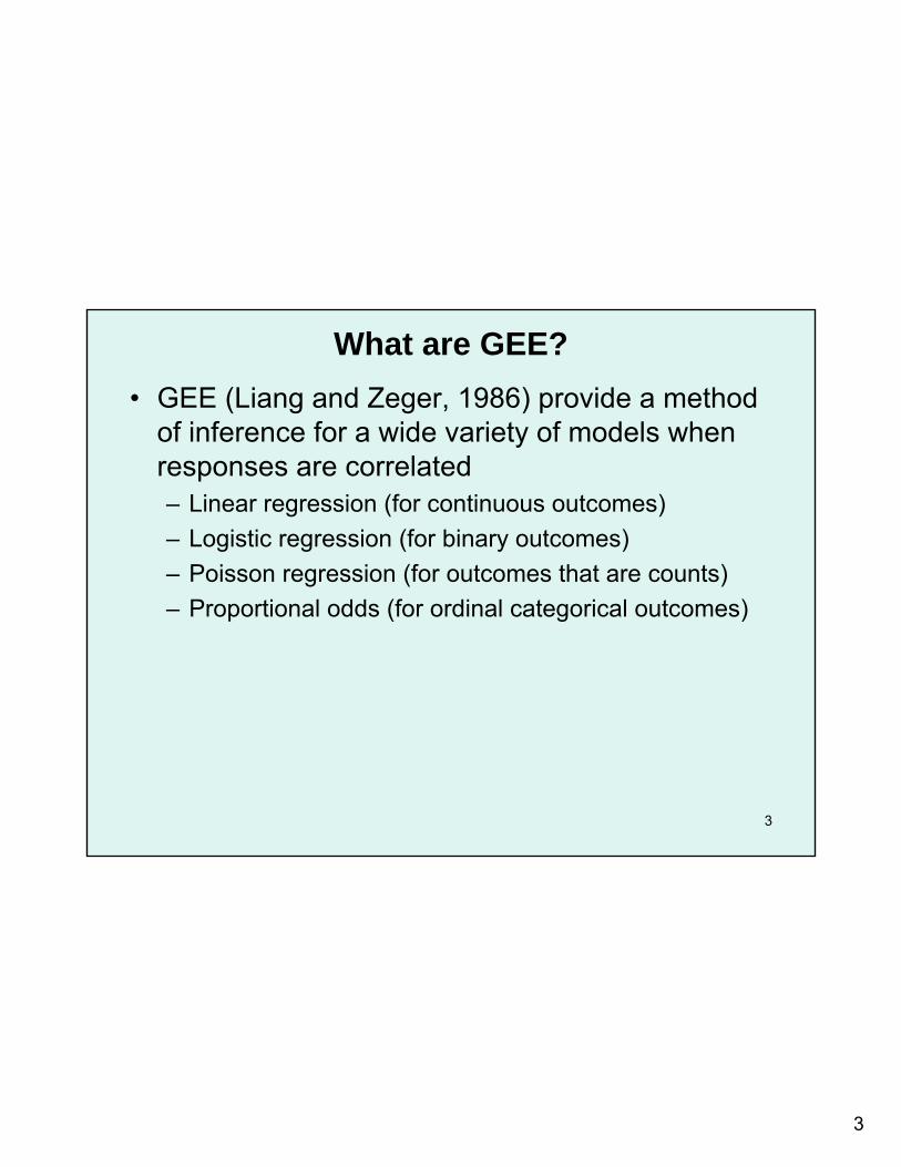
What are GEE?• GEE (Liang and Zeger, 1986) provide a method

of inference for a wide variety of models when responses are correlated– Linear regression (for continuous outcomes)– Logistic regression (for binary outcomes)– Poisson regression (for outcomes that are counts)– Proportional odds (for ordinal categorical outcomes)

4

4

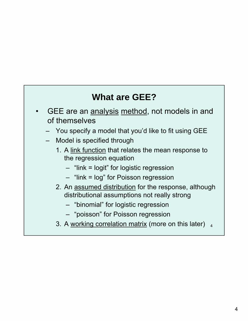
What are GEE?• GEE are an analysis method, not models in and

of themselves– You specify a model that you’d like to fit using GEE– Model is specified through

1. A link function that relates the mean response to the regression equation– “link = logit” for logistic regression– “link = log” for Poisson regression

2. An assumed distribution for the response, although distributional assumptions not really strong– “binomial” for logistic regression– “poisson” for Poisson regression

3. A working correlation matrix (more on this later)

5

5

GEE Benefits• GEE provides many of the same benefits as mixed

models.– Accounts for within-subject/within-cluster correlations– Allows for missing data (but requires stronger

assumption in this regard than mixed models)– Allows for time-varying covariates– Allows for irregularly-timed or mistimed measurements– Range of correlation structures

6

6

Differences Between GEE and Mixed Models

• Mixed models can fit multiple levels of correlations– Ex., longitudinal data from children clustered within

schools• GEE, as implemented in software, is generally

restricted to one level of correlation • Mixed models fit subject-specific models – GEE fit

marginal models (population average).• Mixed models require normality assumptions –

GEE allow for weaker distributional assumptions.

7

7

Differences Between GEE and Mixed Models• Mixed models require assumption that you have

correctly specified the correlation structure – GEE do not.– GEE provide consistent (i.e., asymptotically unbiased)

parameter and standard error estimates even if you do not pick the correct correlation structure.

• Requires number of clusters (or subjects in RCT) to be large (e.g., >50 is probably ok, >100 better)

• As long as “robust” standard errors are used, not “model-based” standard errors

• However, choosing a correlation structure that is closer to the truth improves efficiency of estimates

8

8

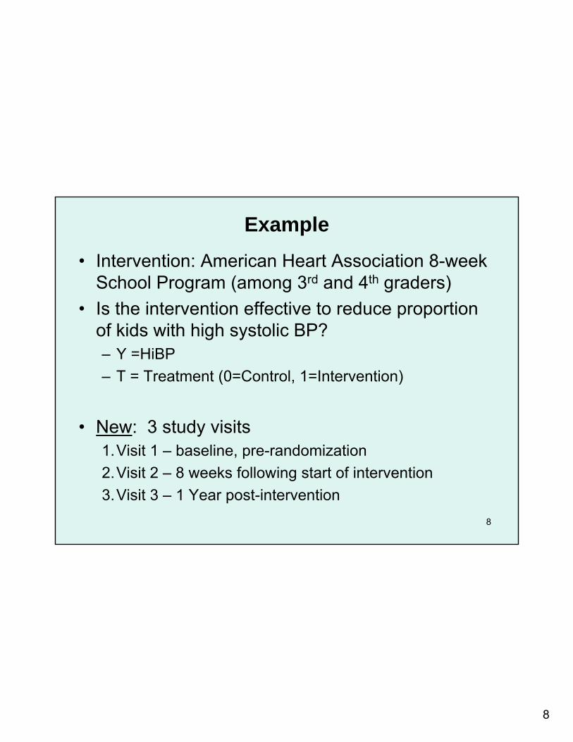
Example• Intervention: American Heart Association 8-week

School Program (among 3rd and 4th graders)• Is the intervention effective to reduce proportion

of kids with high systolic BP?– Y =HiBP– T = Treatment (0=Control, 1=Intervention)

• New: 3 study visits1.Visit 1 – baseline, pre-randomization2.Visit 2 – 8 weeks following start of intervention3.Visit 3 – 1 Year post-intervention

9

9

“Long” Data Structure• Reminder, GEE requires “long” data structure

– One record per observation per subject– True for all standard statistical packages

…F113105…M001202…M002202…M003202

……

Other VARs

…

F102105F101105

SEXTHiBPVISITSTID

10

10

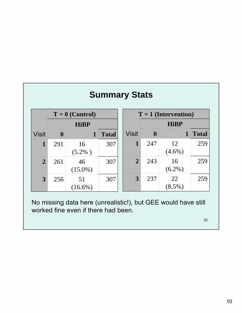
Summary Stats

30751(16.6%)

2563

30746(15.0%)

2612

30716 (5.2% )

2911Total10

HiBPVisit

T = 0 (Control)

25922 (8.5%)

2373

25916 (6.2%)

2432

25912 (4.6%)

2471Total10

HiBPVisit

T = 1 (Intervention)

No missing data here (unrealistic!), but GEE would have still worked fine even if there had been.

11

11

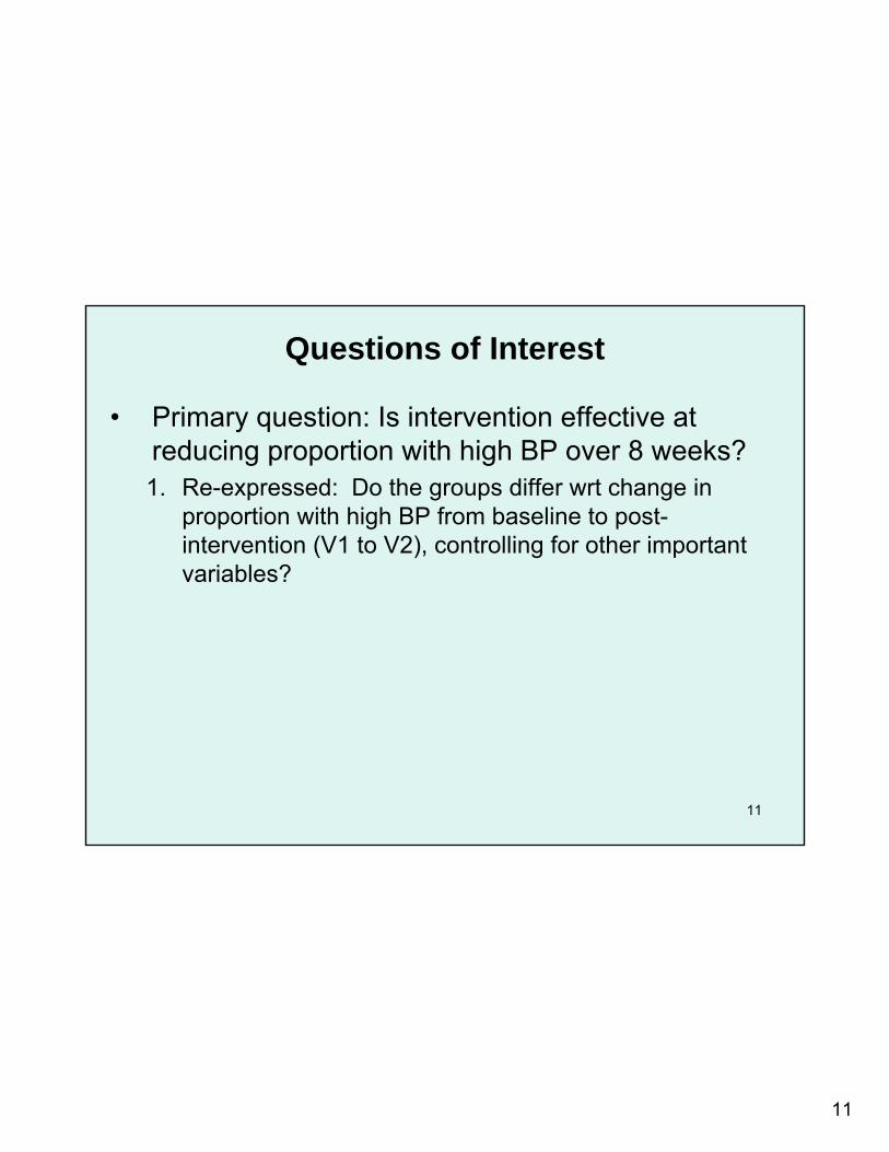
Questions of Interest

• Primary question: Is intervention effective at reducing proportion with high BP over 8 weeks?1. Re-expressed: Do the groups differ wrt change in

proportion with high BP from baseline to post-intervention (V1 to V2), controlling for other important variables?

12

12

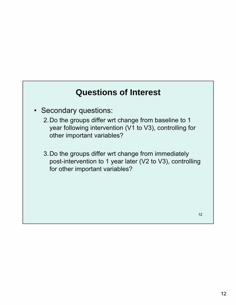
Questions of Interest

• Secondary questions:2.Do the groups differ wrt change from baseline to 1

year following intervention (V1 to V3), controlling for other important variables?

3.Do the groups differ wrt change from immediately post-intervention to 1 year later (V2 to V3), controlling for other important variables?

13

13

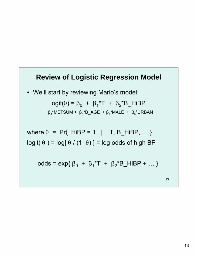
Review of Logistic Regression Model

• We’ll start by reviewing Mario’s model:

logit(θ) = β0 + β1*T + β2*B_HiBP+ β3*METSUM + β4*B_AGE + β5*MALE + β6*URBAN

where θ = Pr{ HiBP = 1 | T, B_HiBP, … }

logit( θ ) = log[ θ / (1- θ) ] = log odds of high BP

odds = exp{ β0 + β1*T + β2*B_HiBP + … }

14

14

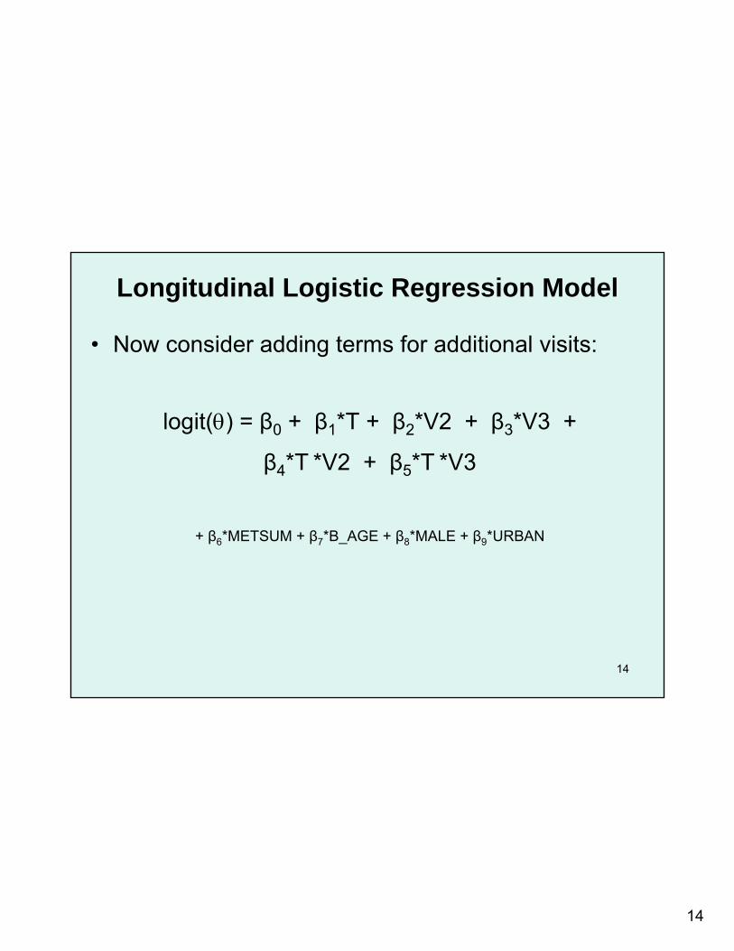
Longitudinal Logistic Regression Model

• Now consider adding terms for additional visits:

logit(θ) = β0 + β1*T + β2*V2 + β3*V3 +

β4*T *V2 + β5*T *V3

+ β6*METSUM + β7*B_AGE + β8*MALE + β9*URBAN

15

15

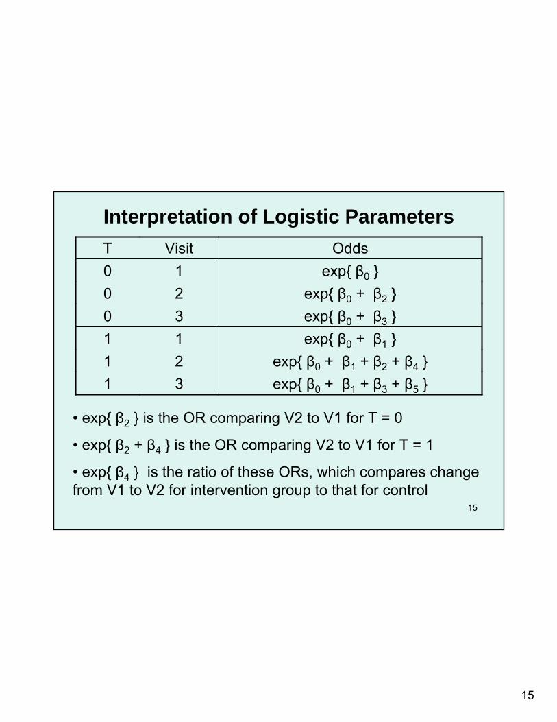
Interpretation of Logistic Parameters

exp{ β0 + β1 + β3 + β5 }31exp{ β0 + β1 + β2 + β4 }21

exp{ β0 + β1 }11exp{ β0 + β3 }30exp{ β0 + β2 }20

exp{ β0 }10OddsVisitT

• exp{ β2 } is the OR comparing V2 to V1 for T = 0

• exp{ β2 + β4 } is the OR comparing V2 to V1 for T = 1

• exp{ β4 } is the ratio of these ORs, which compares change from V1 to V2 for intervention group to that for control

16

16

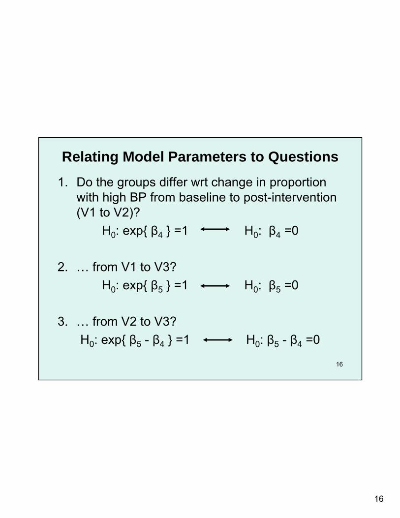
Relating Model Parameters to Questions1. Do the groups differ wrt change in proportion

with high BP from baseline to post-intervention (V1 to V2)?

H0: exp{ β4 } =1 H0: β4 =0

2. … from V1 to V3?H0: exp{ β5 } =1 H0: β5 =0

3. … from V2 to V3?H0: exp{ β5 - β4 } =1 H0: β5 - β4 =0

17

17

Where Does GEE Come In?

• So far, everything we’ve talked about has been a review of standard logistic regression

• So, where does GEE come in?• Keep in mind that the goal of GEE is to account for

within-subject correlations…

18

18

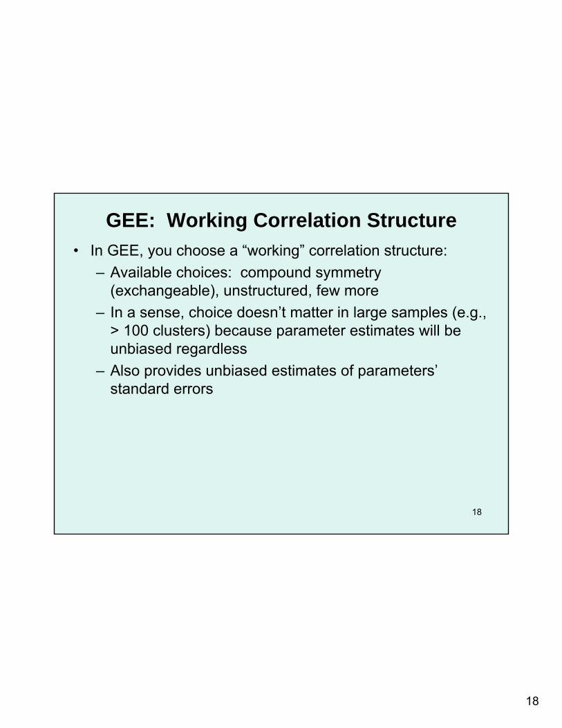
GEE: Working Correlation Structure• In GEE, you choose a “working” correlation structure:

– Available choices: compound symmetry (exchangeable), unstructured, few more

– In a sense, choice doesn’t matter in large samples (e.g., > 100 clusters) because parameter estimates will be unbiased regardless

– Also provides unbiased estimates of parameters’standard errors

19

19

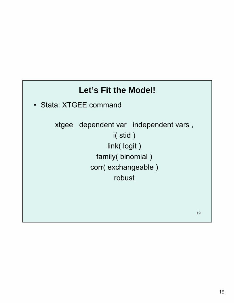
Let’s Fit the Model!• Stata: XTGEE command

xtgee dependent var independent vars , i( stid )

link( logit ) family( binomial )

corr( exchangeable ) robust

20

20

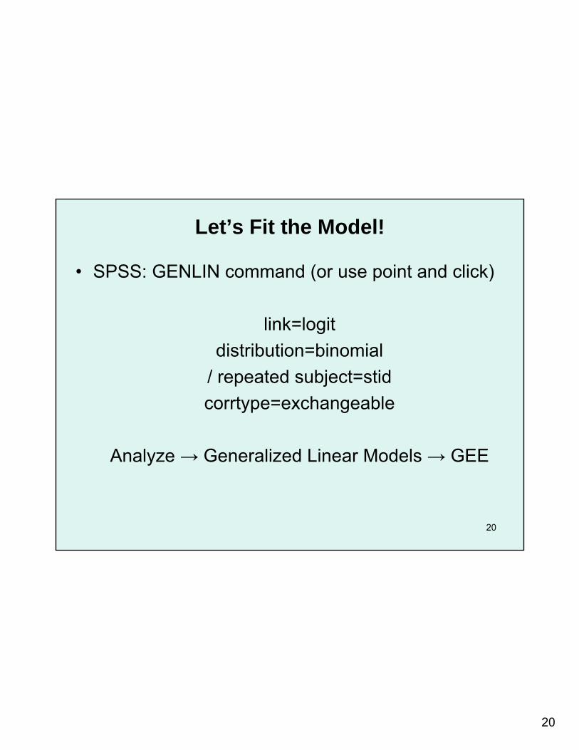
Let’s Fit the Model!

• SPSS: GENLIN command (or use point and click)

link=logitdistribution=binomial

/ repeated subject=stidcorrtype=exchangeable

Analyze → Generalized Linear Models → GEE

21

21

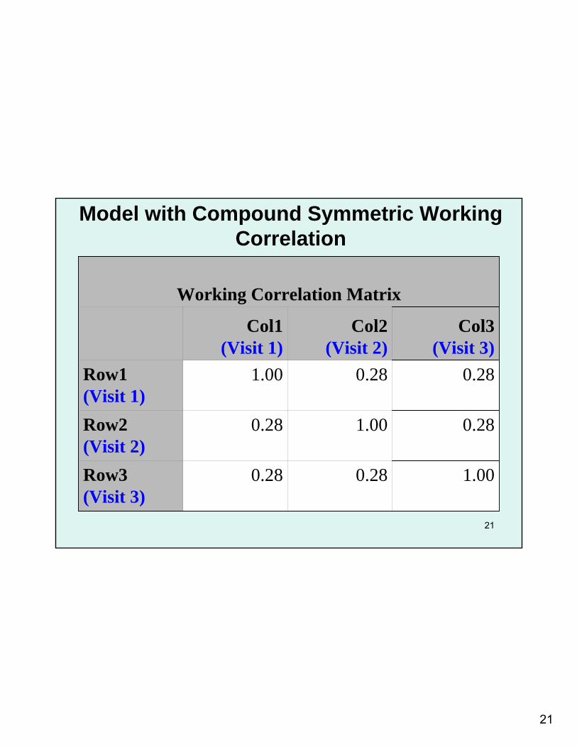
Model with Compound Symmetric Working Correlation

1.000.280.28Row3(Visit 3)

0.281.000.28Row2(Visit 2)

0.280.281.00Row1(Visit 1)

Col3(Visit 3)

Col2(Visit 2)

Col1(Visit 1)

Working Correlation Matrix

22

22

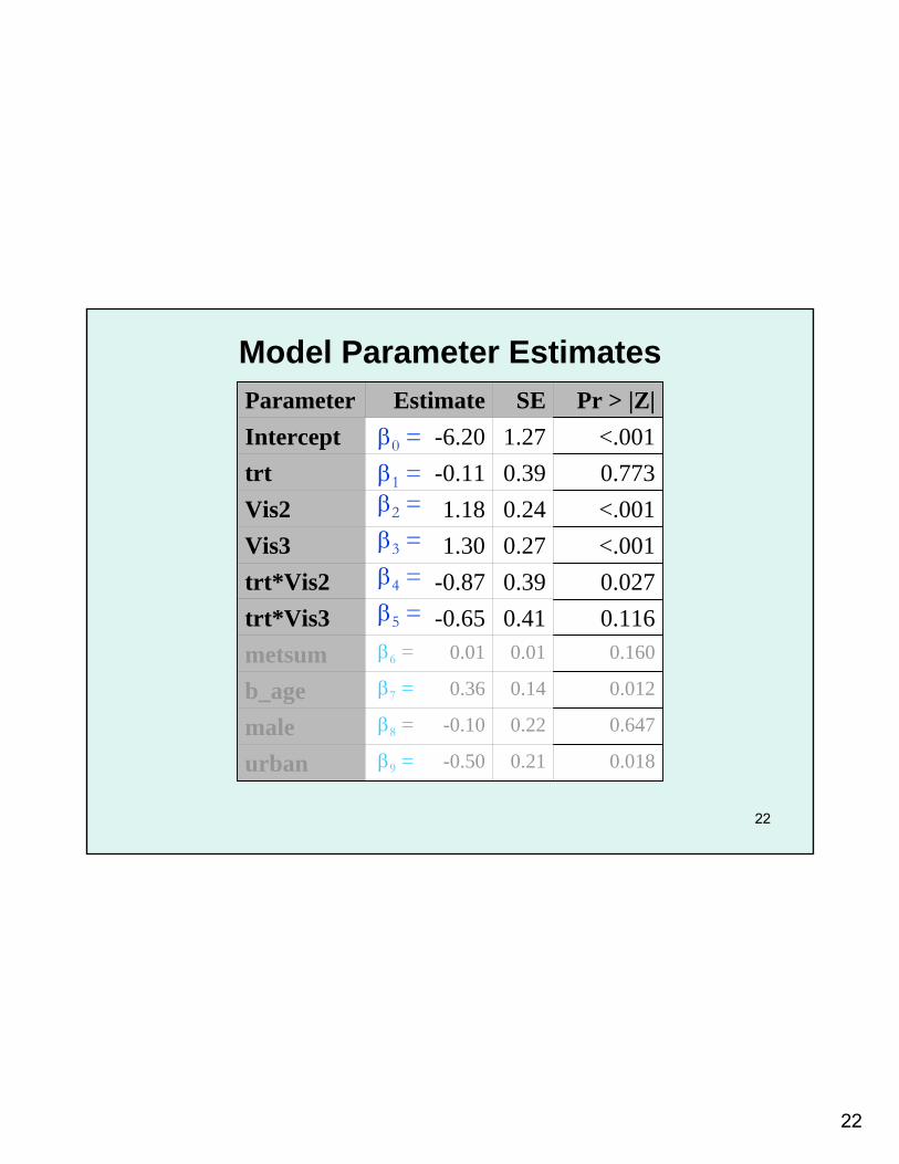
Model Parameter Estimates

0.0180.21-0.50urban

0.6470.22-0.10male

0.0120.140.36b_age

0.1600.010.01metsum0.1160.41-0.65trt*Vis30.0270.39-0.87trt*Vis2<.0010.271.30Vis3<.0010.241.18Vis20.7730.39-0.11trt<.0011.27-6.20Intercept

Pr > |Z|SEEstimateParameterβ0 =β1 =β2 =β3 =β4 =β5 =β6 =

β7 =

β8 =

β9 =

23

23

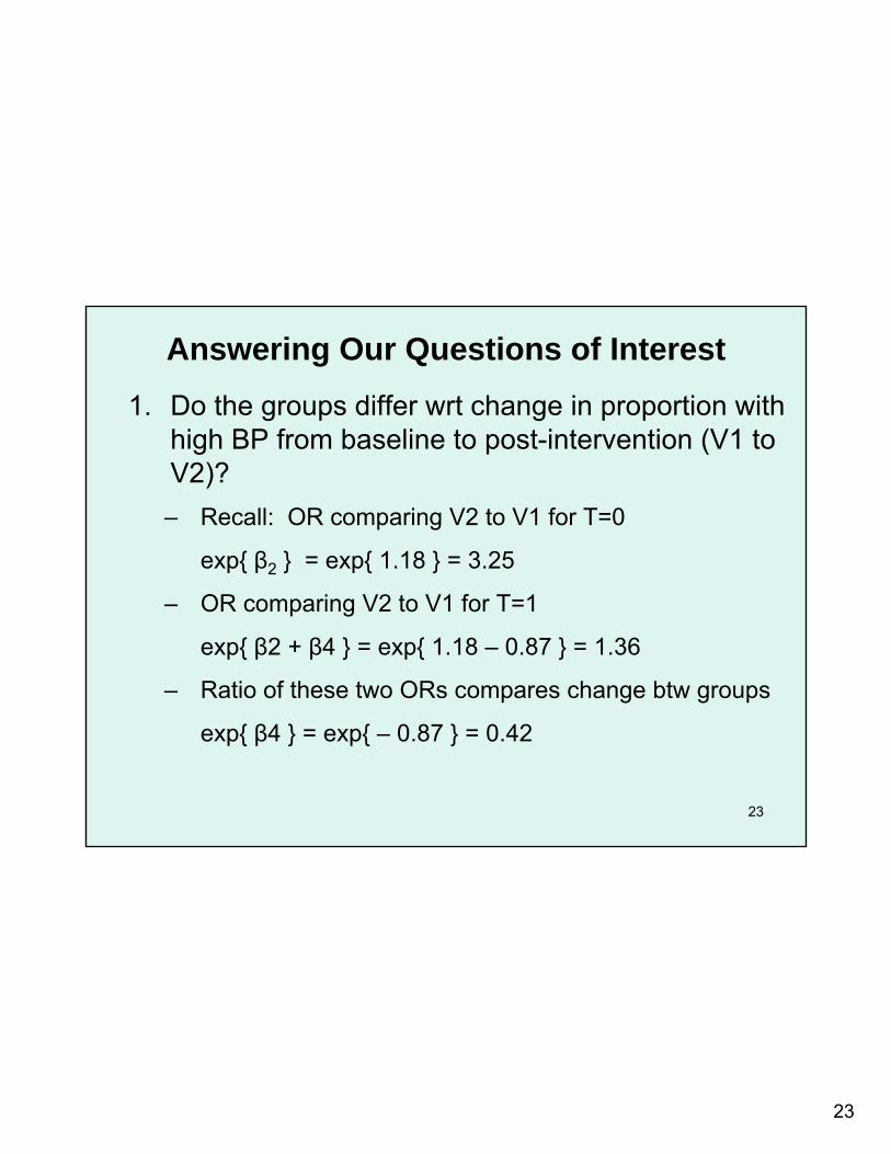
Answering Our Questions of Interest1. Do the groups differ wrt change in proportion with

high BP from baseline to post-intervention (V1 to V2)?– Recall: OR comparing V2 to V1 for T=0

exp{ β2 } = exp{ 1.18 } = 3.25

– OR comparing V2 to V1 for T=1

exp{ β2 + β4 } = exp{ 1.18 – 0.87 } = 1.36

– Ratio of these two ORs compares change btw groups

exp{ β4 } = exp{ – 0.87 } = 0.42

24

24

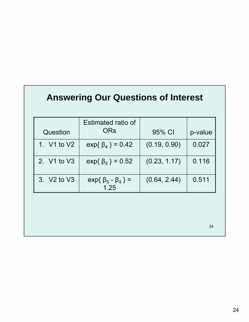
Answering Our Questions of Interest

0.511(0.64, 2.44)exp{ β5 - β4 } = 1.25

3. V2 to V3

0.116(0.23, 1.17)exp{ β5 } = 0.522. V1 to V3

0.027(0.19, 0.90)exp{ β4 } = 0.421. V1 to V2

p-value95% CIEstimated ratio of

ORsQuestion

25

25

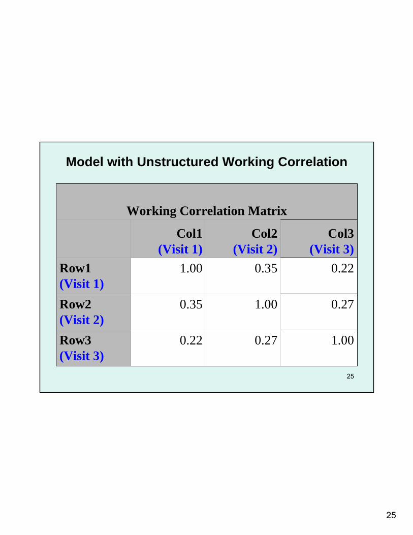
Model with Unstructured Working Correlation

1.000.270.22Row3(Visit 3)

0.271.000.35Row2(Visit 2)

0.220.351.00Row1(Visit 1)

Col3(Visit 3)

Col2(Visit 2)

Col1(Visit 1)

Working Correlation Matrix

26

26

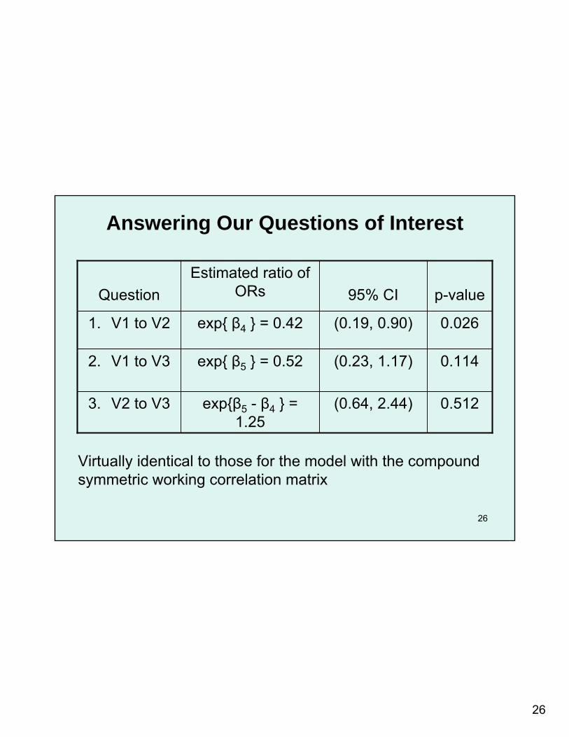
Answering Our Questions of Interest

0.512(0.64, 2.44)exp{β5 - β4 } = 1.25

3. V2 to V3

0.114(0.23, 1.17)exp{ β5 } = 0.522. V1 to V3

0.026(0.19, 0.90)exp{ β4 } = 0.421. V1 to V2

p-value95% CIEstimated ratio of

ORsQuestion

Virtually identical to those for the model with the compound symmetric working correlation matrix

27

27

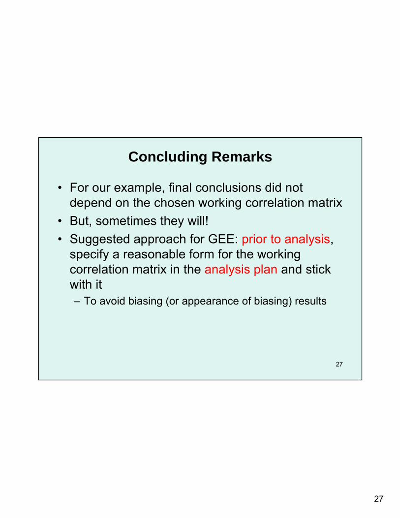
Concluding Remarks

• For our example, final conclusions did not depend on the chosen working correlation matrix

• But, sometimes they will!• Suggested approach for GEE: prior to analysis,

specify a reasonable form for the working correlation matrix in the analysis plan and stick with it– To avoid biasing (or appearance of biasing) results