introduction to 3+1 numerical relativity23. r. e. peierls: quantum theory of solids. introduction to...
TRANSCRIPT

INTERNATIONAL SERIESOF
MONOGRAPHS ON PHYSICS
SERIES EDITORS
J. BIRMAN CITY UNIVERSITY OF NEW YORKS. F. EDWARDS UNIVERSITY OF CAMBRIDGER. FRIEND UNIVERSITY OF CAMBRIDGEM. REES UNIVERSITY OF CAMBRIDGED. SHERRINGTON UNIVERSITY OF OXFORDG. VENEZIANO CERN, GENEVA
International Series of Monographs on Physics
140. M. Alcubierre: Introduction to 3+ 1 numerical relativity139. A. L. Ivanov, S. G. Tikhodeev: Problems of condensed matter physics—quantum
coherence phenomena in electron-hole and coupled matter-light systems138. I. M. Vardavas, F. W. Taylor: Radiation and climate137. A. F. Borghesani: Ions and electrons in liquid helium136. C. Kiefer: Quantum gravity, Second edition135. V. Fortov, I. Iakubov, A. Khrapak: Physics of strongly coupled plasma134. G. Fredrickson: The equilibrium theory of inhomogeneous polymers133. H. Suhl: Relaxation processes in micromagnetics132. J. Terning: Modern supersymmetry131. M. Marino: Chern-Simons theory, matrix models, and topological strings130. V. Gantmakher: Electrons and disorder in solids129. W. Barford: Electronic and optical properties of conjugated polymers128. R. E. Raab, O. L. de Lange: Multipole theory in electromagnetism127. A. Larkin, A. Varlamov: Theory of fluctuations in superconductors126. P. Goldbart, N. Goldenfeld, D. Sherrington: Stealing the gold125. S. Atzeni, J. Meyer-ter-Vehn: The physics of inertial fusion123. T. Fujimoto: Plasma spectroscopy122. K. Fujikawa, H. Suzuki: Path integrals and quantum anomalies121. T. Giamarchi: Quantum physics in one dimension120. M. Warner, E. Terentjev: Liquid crystal elastomers119. L. Jacak, P. Sitko, K. Wieczorek, A. Wojs: Quantum Hall systems118. J. Wesson: Tokamaks, Third edition117. G. Volovik: The Universe in a helium droplet116. L. Pitaevskii, S. Stringari: Bose-Einstein condensation115. G. Dissertori, I.G. Knowles, M. Schmelling: Quantum chromodynamics114. B. DeWitt: The global approach to quantum field theory113. J. Zinn-Justin: Quantum field theory and critical phenomena, Fourth edition112. R. M. Mazo: Brownian motion—fluctuations, dynamics, and applications111. H. Nishimori: Statistical physics of spin glasses and information processing—an
introduction110. N. B. Kopnin: Theory of nonequilibrium superconductivity109. A. Aharoni: Introduction to the theory of ferromagnetism, Second edition108. R. Dobbs: Helium three107. R. Wigmans: Calorimetry106. J. Kubler: Theory of itinerant electron magnetism105. Y. Kuramoto, Y. Kitaoka: Dynamics of heavy electrons104. D. Bardin, G. Passarino: The Standard Model in the making103. G. C. Branco, L. Lavoura, J. P. Silva: CP Violation102. T. C. Choy: Effective medium theory101. H. Araki: Mathematical theory of quantum fields100. L. M. Pismen: Vortices in nonlinear fields99. L. Mestel: Stellar magnetism98. K. H. Bennemann: Nonlinear optics in metals96. M. Brambilla: Kinetic theory of plasma waves94. S. Chikazumi: Physics of ferromagnetism91. R. A. Bertlmann: Anomalies in quantum field theory90. P. K. Gosh: Ion traps88. S. L. Adler: Quaternionic quantum mechanics and quantum fields87. P. S. Joshi: Global aspects in gravitation and cosmology86. E. R. Pike, S. Sarkar: The quantum theory of radiation83. P. G. de Gennes, J. Prost: The physics of liquid crystals73. M. Doi, S. F. Edwards: The theory of polymer dynamics69. S. Chandrasekhar: The mathematical theory of black holes51. C. Møller: The theory of relativity46. H. E. Stanley: Introduction to phase transitions and critical phenomena32. A. Abragam: Principles of nuclear magnetism27. P. A. M. Dirac: Principles of quantum mechanics23. R. E. Peierls: Quantum theory of solids
Introduction to 3+1Numerical Relativity
MIGUEL ALCUBIERRE
Nuclear Sciences Institute,Universidad Nacional Autonoma de Mexico
1

3Great Clarendon Street, Oxford OX2 6DP
Oxford University Press is a department of the University of Oxford.It furthers the University’s objective of excellence in research, scholarship,
and education by publishing worldwide in
Oxford NewYork
Auckland CapeTown Dar es Salaam HongKong KarachiKuala Lumpur Madrid Melbourne MexicoCity Nairobi
NewDelhi Shanghai Taipei Toronto
With offices in
Argentina Austria Brazil Chile CzechRepublic France GreeceGuatemala Hungary Italy Japan Poland Portugal SingaporeSouthKorea Switzerland Thailand Turkey Ukraine Vietnam
Oxford is a registered trade mark of Oxford University Pressin the UK and in certain other countries
Published in the United Statesby Oxford University Press Inc., New York
c© Miguel Alcubierre 2008
The moral rights of the author have been assertedDatabase right Oxford University Press (maker)
First published 2008
All rights reserved. No part of this publication may be reproduced,stored in a retrieval system, or transmitted, in any form or by any means,
without the prior permission in writing of Oxford University Press,or as expressly permitted by law, or under terms agreed with the appropriate
reprographics rights organization. Enquiries concerning reproductionoutside the scope of the above should be sent to the Rights Department,
Oxford University Press, at the address above
You must not circulate this book in any other binding or coverand you must impose this same condition on any acquirer
British Library Cataloguing in Publication Data
Data available
Library of Congress Cataloging in Publication Data
Data available
Printed in Great Britainon acid-free paper by
Biddles Ltd. www.biddles.co.uk
ISBN 978–0–19–920567–7 (Hbk)
1 3 5 7 9 10 8 6 4 2

To Miguel, Raul and Juan,for filling my life with beautiful moments.
To Marıa Emilia and Mili,for being such a wonderful gift.

This page intentionally left blank

ACKNOWLEDGEMENTS
There have been a large number of people that, both directly and indirectly, havehelped me get to a point where I could write this book. First of all, I would liketo thank my mentors and advisors, who put me in the path of studying physicsin general, and relativity in particular. Among them I would like to mention Luisde la Pena and Ana Marıa Cetto who, perhaps somewhat reluctantly, acceptedmy change of heart when I decided to leave the study of the foundations ofquantum mechanics in favor of general relativity. I also thank Eduardo Nahmadfor pointing the way, Bernard F. Schutz for guiding me and being there up tothe present time, and Ed Seidel for always being a friend.
I am also in debt to many friends and colleagues who have been there alongthe road. My old friends from Cardiff, Gabrielle Allen, Gareth Jones, Mario An-tonioletti, Nils Anderson, Kostas Kokkotas, as well as my friends from Potsdam,John Baker, Werner Benger, Steve Brandt, Bernd Bruegmann, Manuela Cam-panelli, Peter Diener, Tony Font, Tom Goodale, Carsten Gundlach, Ian Hawke,Scott Hawley, Frank Herrmann, Daniel Holz, Sasha Husa, Michael Koppitz, GerdLanfermann, Carlos Lousto, Joan Masso, Philippos Papadopoulos, Denis Pollney,Luciano Rezzolla, Alicia Sintes, Nikolaus Stergioulas, Ryoji Takahashi, JonathanThornburg and Paul Walker. There have been other people who have helped mein many ways, either by giving direct answers to my questions, or from whomI have simply learned a lot of what has contributed to this book throughoutthe years, Carles Bona, Matt Choptuik, Eric Gourgoulhon, Pablo Laguna, LuisLehner, Roy Maartens, Mark Miller, Jorge Pullin, Oscar Reula, Olivier Sarbach,Erik Schnetter, Deirdre Shoemaker, Wai-Mo Suen, Manuel Tiglio and Jeff Wini-cour, among others.
I also want to thank my friends and colleagues in Mexico, Alejandro Corichi,Jose Antonio Gonzalez, Francisco S. Guzman, Tonatiuh Matos, Dario Nunez,Luis Urena, Marcelo Salgado, Daniel Sudarsky, Roberto Sussman and HernandoQuevedo. And of course the students of our numerical relativity group, mostof whom have proof-read different sections of the original manuscript, AntonioCastellanos, Juan Carlos Degollado, Cesar Fuentes, Pablo Galaviz, David Mar-tinez, Martha Mendez, Jose Antonio Nava, Bernd Reimann, Milton Ruiz andJose Manuel Torres.
Finally, I wish to thank my editor, Sonke Adlung, who suggested the ideaof writing this book in the first place and has been pushing hard ever since. Iwouldn’t have made it without him.
vii

This page intentionally left blank
PREFACE
General relativity is a highly successful theory. Not only has it radically modifiedour understanding of gravity, space and time, but it also possesses an enormouspredictive power. To date, it has passed with extraordinary precision all theexperimental and observational tests that it has been subjected to. Among itsmore important results are the predictions of exotic objects such as neutronstars and black holes, and the cosmological model of the Big Bang. Also, generalrelativity has predicted the existence of gravitational waves, which might bedetected directly for the first time before this decade is out.
General relativity, for all its conceptual simplicity and elegance, turns outto be in practice a highly complex theory. The Einstein field equations are asystem of ten coupled, non-linear, partial differential equations in four dimen-sions. Written in fully expanded form in a general coordinate system they havethousands of terms. Because of this complexity, exact solutions of the Einsteinequations are only known in cases with high symmetry, either in space or intime: solutions with spherical or axial symmetry, static or stationary solutions,homogeneous and/or isotropic solutions, etc. If we are interested in studyingsystems with astrophysical relevance, which involve strong and dynamical grav-itational fields with little or no symmetry, it is simply impossible to solve thefield equations exactly. The need to study this type of system has given birth tothe field of numerical relativity, which tries to solve the Einstein field equationsusing numerical techniques and complex computational codes.
Numerical relativity appeared as an independent field of research in the mid1960s with the pioneering efforts of Hahn and Lindquist [158], but it wasn’tuntil the mid 1970s when the first truly successful simulations where carried outby Smarr [271] and Eppley [123, 124] in the context of the head-on collision oftwo black holes. At that time, however, the power of the available computerswas very modest, and the simulations that could be performed where limited toeither spherical symmetry or very low resolution axial symmetry. This situationhas changed, and during the decades of the 1980s and 1990s a true revolution hastaken place in numerical relativity. Researchers have studied ever more complexproblems in many different aspects of general relativity, from the simulation ofrotating stars and black holes to the study of topological defects, gravitationalcollapse, singularity structure, and the collisions of compact objects. Maybe themost influential result coming from numerical relativity has been the discovery byChoptuik of critical phenomena in gravitational collapse [98] (for a more recentreview see [153]). A summary of the history of numerical relativity and its morerecent developments can be found in [186].
Numerical relativity has now reached a state of maturity. The appearance of
ix
powerful super-computers, together with an increased understanding of the un-derlying theoretical issues, and the development of robust numerical techniques,has finally allowed the simulation of fully three-dimensional systems with strongand highly dynamic gravitational fields. And all this activity is happening atprecisely the right time, as a new generation of advanced interferometric gravi-tational wave detectors (GEO600, LIGO, VIRGO, TAMA) is finally coming online. The expected gravitational wave signals, however, are so weak that evenwith the amazing sensitivity of the new detectors it will be necessary to extractthem from the background noise. As it is much easier to extract a signal if weknow what to look for, numerical relativity has become badly needed in order toprovide the detectors with precise templates of the type of gravitational wavesexpected from the most common astrophysical sources. We are living a trulyexciting time in the development of this field.
The time has therefore arrived for a textbook on numerical relativity thatcan help as an introduction to this promising field of research. The field hasexpanded in a number of different directions in recent years, which makes writinga fully comprehensive textbook a challenging task. In particular, there are severaldifferent approaches to separating the Einstein field equations in a way thatallows us to think of the evolution of the gravitational field in time. I havedecided to concentrate on one particular approach in this book, namely the3+1 formalism, not because it is the only possibility, but rather because it isconceptually easiest to understand and the techniques associated with it havebeen considerably more developed over the years. To date, the 3+1 formalismcontinues to be used by most researchers in the field. Other approaches, suchas the characteristic and conformal formulations, have important strengths andshow significant promise, but here I will just mention them briefly.
This book is aimed particularly at graduate students, and assumes somebasic familiarity with general relativity. Although the first Chapter gives anintroduction to general relativity, this is mainly a review of some basic concepts,and is certainly not intended to replace a full course on the subject.
Miguel AlcubierreMexico City, September 2007.
x

CONTENTS
1 Brief review of general relativity 11.1 Introduction 11.2 Notation and conventions 21.3 Special relativity 21.4 Manifolds and tensors 71.5 The metric tensor 101.6 Lie derivatives and Killing fields 141.7 Coordinate transformations 171.8 Covariant derivatives and geodesics 201.9 Curvature 251.10 Bianchi identities and the Einstein tensor 281.11 General relativity 281.12 Matter and the stress-energy tensor 321.13 The Einstein field equations 361.14 Weak fields and gravitational waves 391.15 The Schwarzschild solution and black holes 461.16 Black holes with charge and angular momentum 531.17 Causal structure, singularities and black holes 57
2 The 3+1 formalism 642.1 Introduction 642.2 3+1 split of spacetime 652.3 Extrinsic curvature 682.4 The Einstein constraints 712.5 The ADM evolution equations 732.6 Free versus constrained evolution 772.7 Hamiltonian formulation 782.8 The BSSNOK formulation 812.9 Alternative formalisms 87
2.9.1 The characteristic approach 872.9.2 The conformal approach 90
3 Initial data 923.1 Introduction 923.2 York–Lichnerowicz conformal decomposition 92
3.2.1 Conformal transverse decomposition 943.2.2 Physical transverse decomposition 973.2.3 Weighted transverse decomposition 99
3.3 Conformal thin-sandwich approach 101
xi

3.4 Multiple black hole initial data 1053.4.1 Time-symmetric data 1053.4.2 Bowen–York extrinsic curvature 1093.4.3 Conformal factor: inversions and punctures 1113.4.4 Kerr–Schild type data 113
3.5 Binary black holes in quasi-circular orbits 1153.5.1 Effective potential method 1163.5.2 The quasi-equilibrium method 117
4 Gauge conditions 1214.1 Introduction 1214.2 Slicing conditions 122
4.2.1 Geodesic slicing and focusing 1234.2.2 Maximal slicing 1234.2.3 Maximal slices of Schwarzschild 1274.2.4 Hyperbolic slicing conditions 1334.2.5 Singularity avoidance for hyperbolic slicings 136
4.3 Shift conditions 1404.3.1 Elliptic shift conditions 1414.3.2 Evolution type shift conditions 1454.3.3 Corotating coordinates 151
5 Hyperbolic reductions of the field equations 1555.1 Introduction 1555.2 Well-posedness 1565.3 The concept of hyperbolicity 1585.4 Hyperbolicity of the ADM equations 1645.5 The Bona–Masso and NOR formulations 1695.6 Hyperbolicity of BSSNOK 1755.7 The Kidder–Scheel–Teukolsky family 1795.8 Other hyperbolic formulations 183
5.8.1 Higher derivative formulations 1845.8.2 The Z4 formulation 185
5.9 Boundary conditions 1875.9.1 Radiative boundary conditions 1885.9.2 Maximally dissipative boundary conditions 1915.9.3 Constraint preserving boundary conditions 194
6 Evolving black hole spacetimes 1986.1 Introduction 1986.2 Isometries and throat adapted coordinates 1996.3 Static puncture evolution 2066.4 Singularity avoidance and slice stretching 2096.5 Black hole excision 2146.6 Moving punctures 217
xii

6.6.1 How to move the punctures 2176.6.2 Why does evolving the punctures work? 219
6.7 Apparent horizons 2216.7.1 Apparent horizons in spherical symmetry 2236.7.2 Apparent horizons in axial symmetry 2246.7.3 Apparent horizons in three dimensions 226
6.8 Event horizons 2306.9 Isolated and dynamical horizons 234
7 Relativistic hydrodynamics 2387.1 Introduction 2387.2 Special relativistic hydrodynamics 2397.3 General relativistic hydrodynamics 2457.4 3+1 form of the hydrodynamic equations 2497.5 Equations of state: dust, ideal gases and polytropes 2527.6 Hyperbolicity and the speed of sound 257
7.6.1 Newtonian case 2577.6.2 Relativistic case 260
7.7 Weak solutions and the Riemann problem 2647.8 Imperfect fluids: viscosity and heat conduction 270
7.8.1 Eckart’s irreversible thermodynamics 2707.8.2 Causal irreversible thermodynamics 273
8 Gravitational wave extraction 2768.1 Introduction 2768.2 Gauge invariant perturbations of Schwarzschild 277
8.2.1 Multipole expansion 2778.2.2 Even parity perturbations 2808.2.3 Odd parity perturbations 2838.2.4 Gravitational radiation in the TT gauge 284
8.3 The Weyl tensor 2888.4 The tetrad formalism 2918.5 The Newman–Penrose formalism 294
8.5.1 Null tetrads 2948.5.2 Tetrad transformations 297
8.6 The Weyl scalars 2988.7 The Petrov classification 2998.8 Invariants I and J 3038.9 Energy and momentum of gravitational waves 304
8.9.1 The stress-energy tensor for gravitational waves 3048.9.2 Radiated energy and momentum 3078.9.3 Multipole decomposition 313
xiii
9 Numerical methods 3189.1 Introduction 3189.2 Basic concepts of finite differencing 3189.3 The one-dimensional wave equation 322
9.3.1 Explicit finite difference approximation 3239.3.2 Implicit approximation 325
9.4 Von Newmann stability analysis 3269.5 Dissipation and dispersion 3299.6 Boundary conditions 3329.7 Numerical methods for first order systems 3359.8 Method of lines 3399.9 Artificial dissipation and viscosity 3439.10 High resolution schemes 347
9.10.1 Conservative methods 3479.10.2 Godunov’s method 3489.10.3 High resolution methods 350
9.11 Convergence testing 353
10 Examples of numerical spacetimes 35710.1 Introduction 35710.2 Toy 1+1 relativity 357
10.2.1 Gauge shocks 35910.2.2 Approximate shock avoidance 36210.2.3 Numerical examples 364
10.3 Spherical symmetry 36910.3.1 Regularization 37010.3.2 Hyperbolicity 37410.3.3 Evolving Schwarzschild 37810.3.4 Scalar field collapse 383
10.4 Axial symmetry 39110.4.1 Evolution equations and regularization 39110.4.2 Brill waves 39510.4.3 The “Cartoon” approach 399
A Total mass and momentum in general relativity 402
B Spacetime Christoffel symbols in 3+1 language 409
C BSSNOK with natural conformal rescaling 410
D Spin-weighted spherical harmonics 413
References 419
Index 437
xiv
1
BRIEF REVIEW OF GENERAL RELATIVITY
1.1 Introduction
The theory of general relativity, postulated by Einstein at the end of 1915 [120,121], is the modern theory of gravitation. According to this theory, gravity isnot a force as it used to be considered in Newtonian physics, but rather a man-ifestation of the curvature of spacetime. A massive object produces a distortionin the geometry of spacetime around it, and in turn this distortion controls themovement of physical objects. In the words of John A. Wheeler, “matter tellsspacetime how to curve, and spacetime tells matter how to move” [298].
When Einstein introduced special relativity in 1905 it became clear thatNewton’s theory of gravity would have to be modified. The main reason forthis was that Newton’s theory implies that the gravitational interaction wastransmitted between different bodies at infinite speed, in clear contradictionwith one of the fundamental results of special relativity: No physical interactioncan travel faster than the speed of light. It is interesting to note that Newtonhimself was never happy with the existence of this action at a distance, but heconsidered that it was a necessary hypothesis to be used until a more adequateexplanation of the nature of gravity was found. In the years from 1905 to 1915,Einstein focused his efforts on finding such an explanation.
The basic ideas that guided Einstein in his quest towards general relativitywere the principle of general covariance, which says that the laws of physics musttake the same form for all observers, the principle of equivalence, which says thatall objects fall with the same acceleration in a gravitational field regardless oftheir mass, and Mach’s principle, formulated by Ernst Mach at the end of the19th century, which states that the local inertial properties of physical objectsmust be determined by the total distribution of matter in the universe. Theprinciple of general covariance led Einstein to ask for the equations of physics tobe written in tensor form, the principle of equivalence led him to the conclusionthat the natural way to describe gravity was identifying it with the geometry ofspacetime, and Mach’s principle led him to the idea that such geometry shouldbe fixed by the distribution of mass and energy.
The discussion that follows will serve to present some of the basic conceptsof general relativity, but it is certainly not intended to be a detailed introduc-tion to this theory, it is simply too short for that. Readers with no training inrelativity are well advised to read any of the standard textbooks on the subject(for example: Misner, Thorne and Wheeler [206], Wald [295] and Schutz [259]).
1
2 BRIEF REVIEW OF GENERAL RELATIVITY
1.2 Notation and conventions
A comment about notation and conventions is in order. Throughout the book Iwill use the conventions of Misner, Thorne and Wheeler (MTW) [206]. That is,spacetime indices will go from 0 to 3, with 0 representing the time coordinate.Greek indices (α, β, µ, ν, ...) always refer to four-dimensional spacetime and cantake values from 0 to 3, while Latin indices (i, j, k, l, ...) refer to three-dimensionalspace and take values from 1 to 3. The signature of the spacetime metric will betaken to be (−1, +1, +1, +1) (see Section 1.3 below). I will also use Einstein’ssummation convention: Unless otherwise stated, repeated indices are summedover all their possible values.
The system of units used in this book will be the so-called geometric units,in which the speed of light c and Newton’s gravitational constant G are takento be equal to one. Conventional metric (SI) units can always be recovered bymultiplying a given quantity with as many powers of c and G as are neededin each case in order to get back to their correct SI dimensions (for example,making the substitutions t → ct and M → GM/c2). In geometric units allphysical quantities have dimensions of length to some power. In particular, timewill be measured in meters, a meter of time being equal to the time it takeslight to travel one meter (roughly 3× 10⁻⁹ seconds). Mass will also be measuredin meters, with a meter of mass equal to the mass of a point particle that inNewton’s theory has an escape velocity equal to the speed of light at a distanceof two meters (the reason for using two meters instead of one comes from thefactor 2 in the expression for the kinetic energy EK = mv2/2). A meter of massis a fairly large mass, equal to about 1.35×1027 kilograms, i.e. roughly 200 timesthe mass of the Earth (or about 1.4 times the mass of Jupiter). In other words,in these units the mass of the Earth is about half a centimeter, and the mass ofthe Sun about one and a half kilometers.
Finally, for the partial derivatives of a geometric quantity T , I will use in-distinctively the symbols ∂T/∂xµ = ∂µT , and for the covariant derivatives thesymbol ∇µT . When considering covariant derivatives in only three dimensions(as in the 3+1 formalism), I will denote them instead by DiT .
1.3 Special relativity
Before going into general relativity it is important to discuss some of the basicconcepts and results of special relativity. Special relativity was introduced byEinstein in 1905 [118, 119] as a way of reconciling Maxwell’s electrodynamicswith the Galilean principle of relativity that states that the laws of physics arethe same for all inertial observers. It is based on two basic postulates, the firstof which is the principle of relativity itself, and the second the empirical factthat the speed of light is the same for all inertial observers, a fact elevated byEinstein to the status of a physical law. The invariance of the speed of light wasestablished by the null experiment of Michelson and Morley in 1887, thought itis unclear how much influence this experiment had in Einstein’s development of

1.3 SPECIAL RELATIVITY 3
special relativity.1
One can ask what is “special” about special relativity. It is common to hear,even among physicists, that special relativity is special because it can not de-scribe accelerating objects or accelerating observers. This is, of course, quitewrong. Special relativity is essentially a new kinematic framework on which wecan do dynamics, that is, we can study the effects of forces on physical objects,so that accelerations are included all the time. Accelerating observers, or moreto the point accelerating coordinate systems, can also be dealt with, though themathematics becomes more involved. What makes special relativity “special” isthe fact that it assumes the existence of global inertial frames, that is, referenceframes where Newton’s first law holds: Objects free of external forces remainin a state of uniform rectilinear motion. Inertial frames play a crucial role inspecial relativity. In fact, one of the best known results from this theory arethe Lorentz transformations that relate the coordinates in one inertial frame tothose of another. If we assume that we have two inertial frames O and O′, withO′ moving with respect to O with constant speed v along the x axis, then theLorentz transformations are:
t′ = γ (t − vx) , x′ = γ (x − vt) , y′ = y , z′ = z , (1.3.1)
with γ := 1/√
1 − v2 the Lorentz factor. These transformations had been derivedby Lorentz before the work of Einstein as transformations that left Maxwell’sequations invariant. In more compact notation, the Lorentz transformations canbe written as (notice the use of the summation convention)
xµ′= Λµ′
ν xν , (1.3.2)
with xµ = t, x, y, z the coordinates in O, xµ′ the corresponding coordi-nates in O′, and Λµ′
ν the Jacobian matrix:
Λµ′ν =
⎛⎜⎜⎝γ −γv 0 0
−γv γ 0 00 0 1 00 0 0 1
⎞⎟⎟⎠ . (1.3.3)
Notice that the Lorentz transformations mix space and time components, some-thing that was difficult to interpret before special relativity.
The Lorentz transformations have a number of important consequences. Thefirst of these can be easily derived by asking where the events that happen att = 0 according to O end up in the frame O′. From the equations above we seethat these events will have coordinates in O′ such that t′ = −vx′. That is, eventsthat happen at the same time t = 0 in frame O and are thus simultaneous,happen at times that depend on their spatial positions according to O′ and arethen not simultaneous. Simultaneity is therefore relative, or in other words it has
1Einstein did not cite Michelson and Morley in his original papers on relativity [223].
4 BRIEF REVIEW OF GENERAL RELATIVITY
no absolute physical meaning – it is just a convention. Notice that this implies,in particular, that the time order of events is not always fixed: If two eventsare simultaneous in a given inertial frame O, then in a frame O′ moving witha non-zero speed v with respect to O, one of the two events will happen at anearlier time than the other, while in a frame O′′ moving with speed −v withrespect to O it will be the other way around.
The theory of special relativity was put on a more geometric foundationby Herman Minkowski in 1908. Although Einstein initially perceived this as anunnecessarily abstract way of rewriting the same theory, he later realized thatMinkowski’s contribution was in fact crucial for the transition from special togeneral relativity. Minkowski realized that we could rewrite Einstein’s secondpostulate about the invariance of the speed of light in geometric terms if we firstdefined the so-called interval ∆s2 between two events as:2
∆s2 := −∆t2 + ∆x2 + ∆y2 + ∆z2 . (1.3.4)
Einstein’s second postulate then turns out to be equivalent to saying that theinterval defined above between any two events is absolute, that is, all inertial ob-servers will find the same value of ∆s2. This means that we can define a conceptof invariant distance between events, and once we have a measure of distancewe can do geometry. Notice that the ordinary three-dimensional Euclidean dis-tance ∆l2 = ∆x2 + ∆y2 + ∆z2 between two events is not absolute, nor is thetime interval ∆t2, as can be easily seen from the Lorentz transformations. OnlyMinkowski’s four-dimensional spacetime interval is absolute. In Minkowski’s ownwords “... henceforth space by itself, and time by itself, are doomed to fade awayinto mere shadows, and only a kind of union of the two will preserve an inde-pendent reality”.
A crucial property of the spacetime interval defined in (1.3.4) is the fact that,because of the minus sign in front of the first term, it is not positive definite.Rather than this being a drawback, it has an important physical interpretationas it allows us to classify the separation of events according to the sign of ∆s2:
∆s2 > 0 spacelike separation , (1.3.5)∆s2 < 0 timelike separation , (1.3.6)∆s2 = 0 null separation . (1.3.7)
Spacelike separations correspond to events separated in such a way that we wouldhave to move faster than the speed of light to reach one from the other (they areseparated mainly in space), timelike separations correspond to events that can bereached one from the other moving slower than light (they are separated mainlyin time), and null separations correspond to events that can be reached one fromthe other moving precisely at the speed of light. An important consequence of
2The overall sign in the definition of ∆s2 is a matter of convention, and many textbookschoose the opposite sign to the one used here.
1.3 SPECIAL RELATIVITY 5
Causal future
Causal past
ElsewhereElsewhere
time
space
event
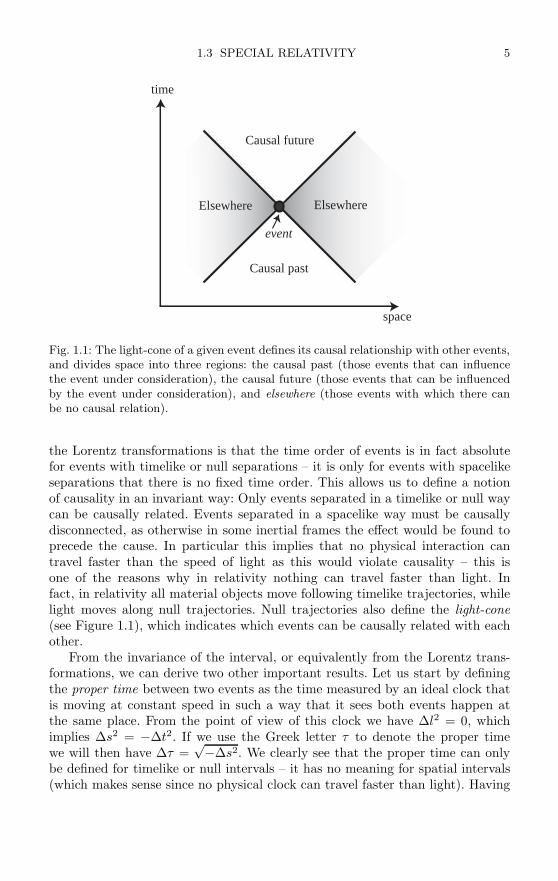
Fig. 1.1: The light-cone of a given event defines its causal relationship with other events,and divides space into three regions: the causal past (those events that can influencethe event under consideration), the causal future (those events that can be influencedby the event under consideration), and elsewhere (those events with which there canbe no causal relation).
the Lorentz transformations is that the time order of events is in fact absolutefor events with timelike or null separations – it is only for events with spacelikeseparations that there is no fixed time order. This allows us to define a notionof causality in an invariant way: Only events separated in a timelike or null waycan be causally related. Events separated in a spacelike way must be causallydisconnected, as otherwise in some inertial frames the effect would be found toprecede the cause. In particular this implies that no physical interaction cantravel faster than the speed of light as this would violate causality – this isone of the reasons why in relativity nothing can travel faster than light. Infact, in relativity all material objects move following timelike trajectories, whilelight moves along null trajectories. Null trajectories also define the light-cone(see Figure 1.1), which indicates which events can be causally related with eachother.
From the invariance of the interval, or equivalently from the Lorentz trans-formations, we can derive two other important results. Let us start by definingthe proper time between two events as the time measured by an ideal clock thatis moving at constant speed in such a way that it sees both events happen atthe same place. From the point of view of this clock we have ∆l2 = 0, whichimplies ∆s2 = −∆t2. If we use the Greek letter τ to denote the proper timewe will then have ∆τ =
√−∆s2. We clearly see that the proper time can onlybe defined for timelike or null intervals – it has no meaning for spatial intervals(which makes sense since no physical clock can travel faster than light). Having
6 BRIEF REVIEW OF GENERAL RELATIVITY
defined the proper time, it is not difficult to show that the interval of time ∆tmeasured between two events in a given inertial frame is related to the propertime between those events in the following way:
∆t = γ∆τ ≥ ∆τ . (1.3.8)
This effect is known as time dilation, and implies that in a given reference frameall moving clocks are measured to go slow. The effect is of course symmetrical:If I measure the clocks of a moving frame as going slow, someone in that framewill measure my clocks as going slow.
Another consequence of the Lorentz transformations is related with the mea-sure of spatial distances. Let us assume that we have a rod of length l as measuredwhen it is at rest (the proper length). If the rod moves with speed v we will mea-sure it as being contracted along the direction of motion. The length L measuredwill be related to l and the speed of the rod v according to:
L = l/γ ≤ l . (1.3.9)
This is known as the Lorentz–Fitzgerald contraction.3
Up until this point we have been considering finite separations in spacetime,but it is more fundamental to consider infinitesimal separations. In the case ofspecial relativity, the fact that spacetime is homogeneous, isotropic and timeindependent allows us to consider finite intervals in an unambiguous way, but ingeneral relativity this will no longer be the case. Because of this, from now onwe will write the spacetime interval of special relativity as
ds2 = −dt2 + dx2 + dy2 + dz2 . (1.3.10)
Moreover, we will use the following compact form
ds2 = ηµν dxµdxν , (1.3.11)
where ηµν is the Minkowski metric tensor defined as
ηµν =
⎛⎜⎜⎝−1 0 0 00 +1 0 00 0 +1 00 0 0 +1
⎞⎟⎟⎠ . (1.3.12)
The infinitesimal interval allows us to think of the length of curves in space-time. For spacelike curves the length is simply defined as the integral of
√ds2
3This contraction had been derived by Lorentz and Fitzgerald before special relativity, butit was considered a dynamical effect due to the interaction between the moving object and theluminiferous aether. However, the fact that the contraction was independent of the physicalproperties of the moving object was difficult to justify. In special relativity the contraction isnot dynamical in origin, but is instead a purely kinematical consequence of the invariance ofthe interval.

1.4 MANIFOLDS AND TENSORS 7
along the curve, while for timelike curves it is defined instead as the integral ofdτ =
√−ds2 and corresponds directly to the time measured by an ideal clockfollowing that trajectory. Null curves, of course, have zero length by definition.We can then easily see that for spacelike curves a straight line between two eventsis the one of minimum length, while for timelike curves the straight line has infact maximum length. In any case straight lines are always extremal curves, alsoknown as geodesics. We can use this fact to rewrite Newton’s first law in geomet-ric terms. Notice first that when thinking about spacetime, Newton’s first lawis simply stated as: Objects free of external forces move along straight timeliketrajectories in spacetime. This simple statement captures both the fact that thetrajectories are straight in three-dimensional space, and also that the motion isuniform. Using the notion of a geodesic we can rewrite this as: Objects free ofexternal forces move along timelike geodesics in spacetime. We can even extendNewton’s first law to light and say: Light rays (photons) in vacuum move alongnull geodesics of spacetime. At this point, we should also mention that it is cus-tomary in relativity to refer to the trajectory of a particle through spacetime asits world-line, so Newton’s first law states that a free particle moves in such away that its world-line corresponds to a geodesic of spacetime.
1.4 Manifolds and tensors
When making the transition from special to general relativity it is important tofirst learn a few basic concepts of differential geometry. Differential geometry isin fact also extremely useful in special relativity, as Minkowski himself showed,but it becomes essential in the general theory.
Differential geometry starts from the notion of a differentiable manifold,which is the formal mathematical way of defining what intuitively is a con-tinuous and smooth space of n dimensions. We are familiar with many manifoldsin physics. For example, Euclidean three-dimensional (3D) space is a 3-manifold,while the spacetime of special relativity is a 4-manifold. But there are many otherinteresting manifolds. The surface of a sphere is a curved, and closed, 2-manifold.The configuration space for a system of two point particles is a 6-manifold, as weneed six coordinates to describe the system. There are also some common mani-folds where there is no notion of distance – the phase space of classical mechanicsis one such manifold. Another interesting manifold is the space of rotations ofa rigid body in three dimensions. Since we can describe any such rotation usingthe three Euler angles, the space of rotations is a 3-manifold, but it has a com-plicated structure: It is not only closed, as rotating an angle of 2π about any axisbrings us back to the original situation, but it also has a non-trivial topology.
Mathematically, a manifold M is defined as a space that can be covered bya collection of charts, that is, one-to-one mappings from n to M . Euclidean3D space can be clearly covered by one such mapping from 3 in a trivial way,while for the surface of a sphere we actually need at least two mappings from 2(standard maps fail at two points, namely the poles, but a stereographic mapfails at only one point, so we need two of those). In more physical language, a

8 BRIEF REVIEW OF GENERAL RELATIVITY
mapping is nothing more than a set of coordinates that label the different pointsin M . Notice that a coordinate system on a given patch of M is not unique,coordinate systems are in fact arbitrary.
Once we have a manifold, we can consider curves in this manifold defined asfunctions from a segment of the real line into the manifold. It is important todistinguish between the image of a curve (i.e. its trajectory), and the curve itself:The curve is the function and contains information both about which points onM we are traversing, and how fast we are moving with respect to the parameter.In terms of a set of coordinates xα on M , a curve is represented as
xα = xα(λ) , λ ∈ . (1.4.1)
Notice that a change of coordinates will alter the explicit functional form above,but will not alter the curve itself. Working with coordinates helps to make manyconcepts explicit, but we should always be careful not to confuse the coordinaterepresentation of a geometric object with the object itself.
Vectors are defined as derivative operators along a given curve. The precisedefinition is somewhat abstract, and although this is certainly convenient froma mathematical point of view, here we will limit ourselves to working with thecomponents of a vector. The components of a vector v tangent to a curve xα(λ)are given simply by
vα = dxα/dλ . (1.4.2)
Vectors are defined at a given point, and on that point they form a vectorspace known as the tangent space of M (one should really think of vectors asrepresenting only infinitesimal displacements on M).
Since vectors form a vector space, we can always represent them as linearcombinations of some basis vectors eα, where here α is an index that identifiesthe different vectors in the basis and not their components. For example, for anarbitrary vector v we have
v = vαeα . (1.4.3)
A common basis choice (though certainly not the only possibility) is the so-called coordinate basis for which we take as the basis those vectors that aretangent to the coordinate lines, using as parameters the coordinates themselves.It is precisely in this basis that the components of a vector are given as definedabove. From here on we will always work with the coordinate basis (but seeChapter 8 where we will discuss the use of a non-coordinate basis known as atetrad frame).
Let us now consider functions of vectors on the tangent space. A linear, real-valued function of one vector is called a one-form. We will denote one-formswith a tilde and write the action of a one-form q on a vector v as q(v).4 It is not
4The name one-form comes from the calculus of differential forms and the notion of exteriorderivatives. Forms are very important in the theory of integration in manifolds. Here, however,we will not consider the calculus of forms, and we will take “one-form” to be just a name –
1.4 MANIFOLDS AND TENSORS 9
difficult to show that one-forms also form a vector space of the same dimensionas that of the manifold – this is known as the dual tangent space, and for thisreason one-forms are often called co-vectors.
The components of a one-form are defined as the value of the one-form actingon the basis vectors:
qα := q(eα) . (1.4.4)
Notice that while the components of a vector are represented with indices up,those of a one-form have the indices down.
We can also define a basis for the space of one-forms, known as the dual basisωα, and defined as those one-forms such that, when acting on the basis vectorseα, give us the identity matrix
ωα(eβ) = δαβ , (1.4.5)
where δαβ is the Kronecker delta. The dual basis has one very important property,
namely that the components of a one-form defined above are precisely the onesthat allow us to write the one-form in terms of the dual basis:
q = qαωα . (1.4.6)
In terms of the basis of vectors and one-forms, the action of an arbitraryone-form q on a vector v can be represented as:
q(v) = qαωα(vβeβ) = qαvβωα(eβ) = qαvβδαβ = qαvα . (1.4.7)
where we have used the linearity of the one-forms and the definition of the dualbasis. The last expression shows that the action of q on v is just the sum of thecomponents of q times the components of v. This operation is called a contraction,and it gives us a real number that is in fact independent of the coordinate systemor basis we are using.
One-forms and vectors are dual in one other respect: We can invert the defi-nition and define a vector v as a real-valued function of a one-form, namely thefunction that, given a one-form q, gives us back the real number q(v). We canthen generalize this idea and think of real-valued functions of m one-forms andn vectors that are linear in all their arguments. This is what defines a tensor oftype
„mn
«. The components of a tensor are then just the values of the tensor
applied to the elements of the basis of vectors and one-forms. For example, fora tensor T of
„22
«type, we have
T αβµν := T
(ωα, ωβ ;eµ, eν
). (1.4.8)
We can then think of vectors and one-forms as„
10
«and
„01
«tensors respectively.
Just like vectors, tensors are defined at each point, but we can easily constructtensor fields by a rule that gives a tensor at each point of the manifold M .
readers interested in this subject can consult any standard text on differential geometry (seee.g. [258]).

10 BRIEF REVIEW OF GENERAL RELATIVITY
A particularly important one-form field is the gradient of a scalar function.Consider a function f from M into the real numbers. This is called a scalarfunction and can be thought of as a
„00
«tensor field. The gradient of f is denoted
by df , and is the one-form with components ∂f/∂xα ≡ ∂αf . The notation usedhere should already make us pay attention – the indices for the components ofthe gradient are down, which suggests that it is a one-form and not a vector.It becomes clear that it is a one-form since we can apply it to an arbitraryvector v to get a real number, namely vα∂αf , which is nothing more than thedirectional derivative of f along the vector v. We will see below that the gradientalso transforms with the rules of a one-form and not of a vector.
An important characteristic of tensors has to do with their symmetry prop-erties with respect to exchange of their arguments. We say that a tensor iscompletely symmetric if it remains the same with respect to exchange of anypair of arguments. Similarly, a tensor is said to be completely antisymmetric ifit changes sign with respect to exchange of any pair of arguments.5 The sym-metric and antisymmetric parts of an arbitrary tensor can be easily constructedby adding together all possible permutations of their arguments with appropri-ate signs: all positive for the symmetric part, and positive or negative for theantisymmetric part depending on whether the permutation is even or odd. Forexample, for a
„02
«tensor T we have:
T(αβ) :=12!
(Tαβ + Tβα) , (1.4.9)
T[αβ] :=12!
(Tαβ − Tβα) , (1.4.10)
where the round and square brackets are standard notation for the symmetricand antisymmetric parts, respectively, and the 1/2! is a normalization factor.Generalizations to tensors of higher rank are straightforward. The symmetriesof tensors are quite important in general relativity where many of the mostimportant tensors have very specific symmetry properties.
1.5 The metric tensorAs we have seen, the crucial contribution of Minkowski to the theory of relativitywas the realization that there exists a measure of invariant distance between twoevents in four-dimensional spacetime. More generally, in a given manifold M anotion of distance is given by the existence of a symmetric, non-degenerate,
„02
«
tensor g that defines the dot or scalar product between two vectors
g(v, u) ≡ v · u = gαβ vαuβ , (1.5.1)
with gαβ the components of g. By non-degenerate we mean that if we have avector w such that g(w,v) = 0 for all v, then we must necessarily have that
5A p-form is defined as a completely antisymmetric„
0p
«tensor.
1.5 THE METRIC TENSOR 11
w = 0 (this also implies that the components gαβ form an invertible matrix).The tensor g giving this scalar product is called the metric tensor, and allows usto define the magnitude or norm of a vector as
|v|2 := g(v,v) = v · v = gαβ vαvβ . (1.5.2)
In particular, we can calculate the magnitude of the displacement vector dxbetween two infinitesimally close points in the manifold as
ds2 = gαβ dxαdxβ , (1.5.3)
which allows us to define a notion of distance between these two points. Notall manifolds have such a metric tensor defined on them, the obvious physicalexample of a manifold with no metric being the phase space of classical mechan-ics. The metric tensor gives an extra degree of structure to a manifold. In theparticular case of special relativity we do in fact have such a notion of distance,with the metric tensor g given by Minkowski’s interval: gαβ = ηαβ . This alsomeans that in special relativity we can not only calculate distances, but in factwe can also construct the scalar product of two arbitrary vectors.
As already mentioned, the metric of special relativity is not positive definite.In general, the signature of a metric is given by the signs of the eigenvalues ofits matrix of components. We call a positive definite metric, i.e. one with alleigenvalues positive, Euclidean, while a metric like the one of special relativitywith signature (−, +, +, +) is called Lorentzian. For a Lorentzian metric like theone in relativity, we classify vectors in the same way as intervals according tothe sign of their magnitude and talks about spacelike, null and timelike vectors.
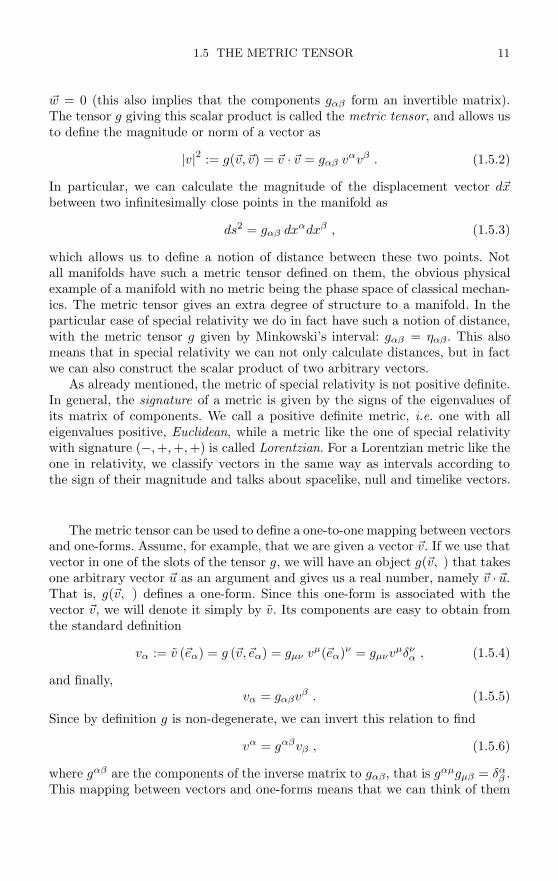
The metric tensor can be used to define a one-to-one mapping between vectorsand one-forms. Assume, for example, that we are given a vector v. If we use thatvector in one of the slots of the tensor g, we will have an object g(v, ) that takesone arbitrary vector u as an argument and gives us a real number, namely v · u.That is, g(v, ) defines a one-form. Since this one-form is associated with thevector v, we will denote it simply by v. Its components are easy to obtain fromthe standard definition
vα := v (eα) = g (v,eα) = gµν vµ(eα)ν = gµνvµδνα , (1.5.4)
and finally,vα = gαβvβ . (1.5.5)
Since by definition g is non-degenerate, we can invert this relation to find
vα = gαβvβ , (1.5.6)
where gαβ are the components of the inverse matrix to gαβ, that is gαµgµβ = δαβ .
This mapping between vectors and one-forms means that we can think of them
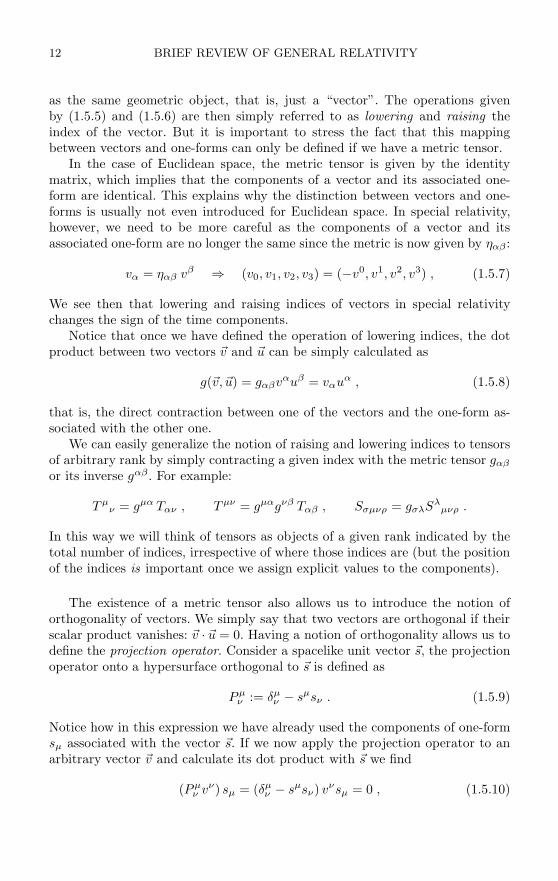
12 BRIEF REVIEW OF GENERAL RELATIVITY
as the same geometric object, that is, just a “vector”. The operations givenby (1.5.5) and (1.5.6) are then simply referred to as lowering and raising theindex of the vector. But it is important to stress the fact that this mappingbetween vectors and one-forms can only be defined if we have a metric tensor.
In the case of Euclidean space, the metric tensor is given by the identitymatrix, which implies that the components of a vector and its associated one-form are identical. This explains why the distinction between vectors and one-forms is usually not even introduced for Euclidean space. In special relativity,however, we need to be more careful as the components of a vector and itsassociated one-form are no longer the same since the metric is now given by ηαβ :
vα = ηαβ vβ ⇒ (v0, v1, v2, v3) = (−v0, v1, v2, v3) , (1.5.7)
We see then that lowering and raising indices of vectors in special relativitychanges the sign of the time components.
Notice that once we have defined the operation of lowering indices, the dotproduct between two vectors v and u can be simply calculated as
g(v, u) = gαβvαuβ = vαuα , (1.5.8)
that is, the direct contraction between one of the vectors and the one-form as-sociated with the other one.
We can easily generalize the notion of raising and lowering indices to tensorsof arbitrary rank by simply contracting a given index with the metric tensor gαβ
or its inverse gαβ . For example:
T µν = gµα Tαν , T µν = gµαgνβ Tαβ , Sσµνρ = gσλSλ
µνρ .
In this way we will think of tensors as objects of a given rank indicated by thetotal number of indices, irrespective of where those indices are (but the positionof the indices is important once we assign explicit values to the components).
The existence of a metric tensor also allows us to introduce the notion oforthogonality of vectors. We simply say that two vectors are orthogonal if theirscalar product vanishes: v · u = 0. Having a notion of orthogonality allows us todefine the projection operator. Consider a spacelike unit vector s, the projectionoperator onto a hypersurface orthogonal to s is defined as
P µν := δµ
ν − sµsν . (1.5.9)
Notice how in this expression we have already used the components of one-formsµ associated with the vector s. If we now apply the projection operator to anarbitrary vector v and calculate its dot product with s we find
(P µν vν) sµ = (δµ
ν − sµsν) vνsµ = 0 , (1.5.10)
1.5 THE METRIC TENSOR 13
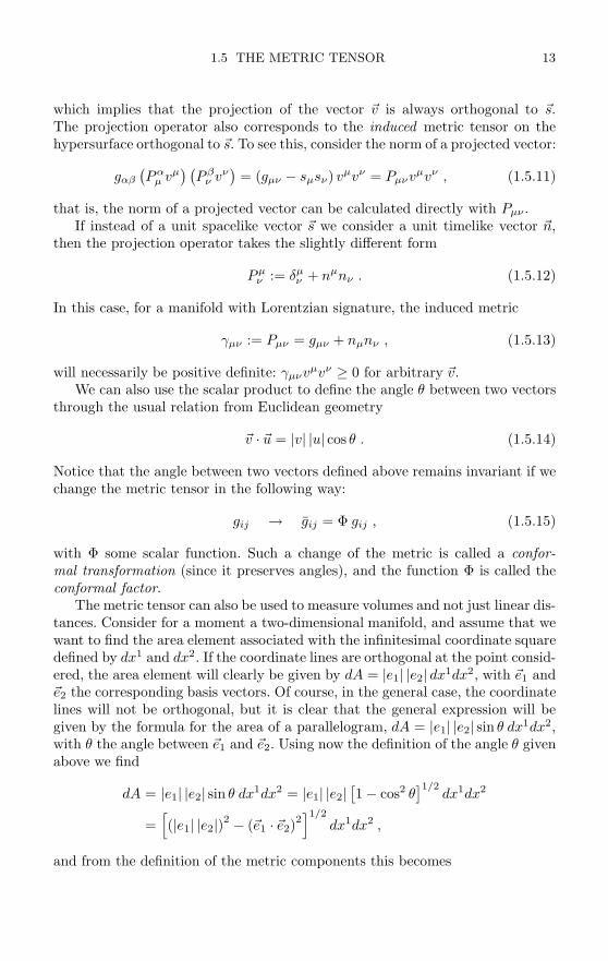
which implies that the projection of the vector v is always orthogonal to s.The projection operator also corresponds to the induced metric tensor on thehypersurface orthogonal to s. To see this, consider the norm of a projected vector:
gαβ
(Pα
µ vµ) (
P βν vν
)= (gµν − sµsν) vµvν = Pµνvµvν , (1.5.11)
that is, the norm of a projected vector can be calculated directly with Pµν .If instead of a unit spacelike vector s we consider a unit timelike vector n,
then the projection operator takes the slightly different form
Pµν := δµ
ν + nµnν . (1.5.12)
In this case, for a manifold with Lorentzian signature, the induced metric
γµν := Pµν = gµν + nµnν , (1.5.13)
will necessarily be positive definite: γµνvµvν ≥ 0 for arbitrary v.We can also use the scalar product to define the angle θ between two vectors
through the usual relation from Euclidean geometry
v · u = |v| |u| cos θ . (1.5.14)
Notice that the angle between two vectors defined above remains invariant if wechange the metric tensor in the following way:
gij → gij = Φ gij , (1.5.15)
with Φ some scalar function. Such a change of the metric is called a confor-mal transformation (since it preserves angles), and the function Φ is called theconformal factor.
The metric tensor can also be used to measure volumes and not just linear dis-tances. Consider for a moment a two-dimensional manifold, and assume that wewant to find the area element associated with the infinitesimal coordinate squaredefined by dx1 and dx2. If the coordinate lines are orthogonal at the point consid-ered, the area element will clearly be given by dA = |e1| |e2| dx1dx2, with e1 ande2 the corresponding basis vectors. Of course, in the general case, the coordinatelines will not be orthogonal, but it is clear that the general expression will begiven by the formula for the area of a parallelogram, dA = |e1| |e2| sin θ dx1dx2,with θ the angle between e1 and e2. Using now the definition of the angle θ givenabove we find
dA = |e1| |e2| sin θ dx1dx2 = |e1| |e2|[1 − cos2 θ
]1/2dx1dx2
=[(|e1| |e2|)2 − (e1 · e2)2
]1/2dx1dx2 ,
and from the definition of the metric components this becomes

14 BRIEF REVIEW OF GENERAL RELATIVITY
dA =[g11g22 − (g12)
2]1/2
= [det(g)]1/2 dx1dx2 ,
where det(g) is the determinant of the matrix of metric components. It turnsout that this relation can be generalized to an arbitrary number of dimensions,and the volume element of an n-dimensional manifold is always given by
dV = |g|1/2 dx1 · · ·dxn . (1.5.16)
In the last expression we have introduced the standard convention of using simplyg to denote the determinant of the metric. Also, the absolute value is there toallow for the possibility of having a non-positive definite metric.
A particularly useful tensor related to the determinant of the metric g isthe Levi–Civita completely antisymmetric tensor ε, which in four dimensions isdefined as6
εαβµν =
⎧⎨⎩+ |g|1/2 for even permutations of 0,1,2,3− |g|1/2 for odd permutations of 0,1,2,3
0 if any indices are repeated(1.5.17)
The factor |g|1/2 guarantees that, in an orthonormal frame, the components of εare always ±1. We can define the Levi–Civita tensor with two or three indices byconsidering lower dimensional manifolds within our four-dimensional spacetime,but notice that the Levi–Civita tensor with five indices is identically zero.
1.6 Lie derivatives and Killing fields
Like vectors, tensors are defined at a specific point on a manifold, and althoughwe can define tensor fields easily enough there is no natural way to comparetensors at different points in the manifold since they live on different spaces. Thismeans, in particular, that there is no natural notion of the derivative of a tensor,since that requires us to compare the values of a tensor field at nearby pointsin the manifold. We will see in the next Sections that, given a metric, we canintroduce a notion of derivative known as the covariant derivative. However, thereis a more primitive notion of derivative that does not depend on the existence ofa metric and that is often quite useful. This is known as the Lie derivative, andis based on the existence of a vector field v defined on the manifold.
Consider a smooth vector field v on a region of a manifold. The congruenceof integral curves of this vector field defines a mapping φ of the manifold intoitself – we simply identify a given point p with another point q = φλ(p) that lieson the same integral curve as p at a distance λ, as defined by the change in the
6In an n-dimensional manifold, the Levi–Civita tensor is strictly speaking an n-form knownas the natural volume element. It is also only defined for orientable manifolds, and the standarddefinition corresponds to a right handed basis.
1.6 LIE DERIVATIVES AND KILLING FIELDS 15
v congruence
u integral curve
u integral curve
u dragged curvep
q
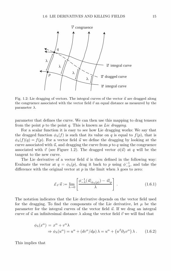
Fig. 1.2: Lie dragging of vectors. The integral curves of the vector u are dragged alongthe congruence associated with the vector field v an equal distance as measured by theparameter λ.
parameter that defines the curve. We can then use this mapping to drag tensorsfrom the point p to the point q. This is known as Lie dragging.
For a scalar function it is easy to see how Lie dragging works: We say thatthe dragged function φλ(f) is such that its value on q is equal to f(p), that isφλ(f)(q) = f(p). For a vector field u we define the dragging by looking at thecurve associated with u, and dragging the curve from p to q using the congruenceassociated with v (see Figure 1.2). The dragged vector φ(u) at q will be thetangent to the new curve.
The Lie derivative of a vector field u is then defined in the following way:Evaluate the vector at q = φλ(p), drag it back to p using φ−1
−λ, and take thedifference with the original vector at p in the limit when λ goes to zero:
£v u := limλ→0
[φ−1−λ(u|φλ(p)
) − u|pλ
]. (1.6.1)
The notation indicates that the Lie derivative depends on the vector field usedfor the dragging. To find the components of the Lie derivative, let µ be theparameter for the integral curves of the vector field u. If we drag an integralcurve of u an infinitesimal distance λ along the vector field v we will find that
φλ(xα) = xα + vαλ
⇒ φλ(uα) = uα + (dvα/dµ)λ = uα +(uβ∂βvα
)λ . (1.6.2)
This implies that
16 BRIEF REVIEW OF GENERAL RELATIVITY
£v uα = limλ→0
⎡⎣ uα|φλ(p)− λ
(uβ∣∣φλ(p)
∂βvα)− uα|p
λ
⎤⎦= duα/dλ − uβ∂βvα
= vβ∂βuα − uβ∂βvα . (1.6.3)
If we now define the Lie bracket or commutator of two vectors as
[v, u]α := vβ∂βuα − uβ∂βvα , (1.6.4)
then we find that£v u = [v, u] . (1.6.5)
That is, the Lie derivative of u with respect to v is nothing more than thecommutator of v and u.
Once we know how to drag vectors, we can also drag one-forms by just askingfor the value of the dragged one-form when applied to the dragged vector tobe equal to the value of the original one-form applied to the original vector:φλ(ω)(φλ(u)) = ω(u). In the same way we can drag tensors of arbitrary rank.We can then define the Lie derivative of tensors in an analogous way to that ofvectors. For a one-form ω we find
£v ωα = vβ∂βωα + ωβ∂αvβ . (1.6.6)
We can do the same for tensors of arbitrary rank, just adding one more term foreach index, with the adequate sign. For example
£v T αβ = vµ∂µT α
β − T µβ∂µvα + T α
µ∂βvµ . (1.6.7)
There is an important property of Lie derivatives that helps considerablywith their interpretation. Assume that we adapt one of our coordinates, say x1,to the integral curves of the vector field v. In that case we have that x1 = λ ande1 = v, which implies vα = δα
1 . It is then easy to see that the Lie derivative of atensor T of arbitrary rank will simplify to
£v T αβ...µν... = ∂1T
αβ...µν... . (1.6.8)
This shows that the Lie derivative is a way to write partial derivatives along thedirection of a given vector field in a way that is independent of the coordinates.
A particularly important application of the Lie derivative is related to thepossible symmetries of a manifold that has a metric tensor defined on it. We saythat the manifold has a specific symmetry if the metric is invariant under Liedragging with respect to some vector field ξ, that is, if we have
£ξ g = 0 . (1.6.9)
1.7 COORDINATE TRANSFORMATIONS 17
From the expression for the Lie derivative of a tensor we find that this implies
ξµ ∂µgαβ + gαµ ∂βξµ + gµβ ∂αξµ = 0 . (1.6.10)
If given a metric gµν there exists a vector field ξ that satisfies the above equation,then ξ is called a Killing field. It is easy to see that the existence of a Killingfield implies a symmetry of the manifold: Assume as before that the coordinatex1 is adapted to the integral curves of ξ, the condition above then reduces to
∂1gαβ = 0 , (1.6.11)
so the components of the metric tensor are in fact independent of the coordinatex1. We will come back to the condition for the existence of a Killing field inSection 1.8, where we will rewrite it in a more standard way.
1.7 Coordinate transformations
Up until this point we have assumed that we are given a specific coordinatesystem xα and its associated coordinate basis eα. However, we must alsoconsider what happens when we transform to a different set of coordinates. Thisis important as coordinates are in fact arbitrary labels for points in a manifold,and we might want to choose different coordinates under different circumstances.For example, in the particular case of special relativity, we might wish to usethe coordinates associated with a given inertial frame, or those associated witha different inertial frame and related to the first ones via the Lorentz transfor-mations.
More generally, we wish to consider arbitrary changes of coordinates of theform xα = f α(xβ). It is easy to see that under this change of coordinates thecomponents of the displacement vector transform as
dxα =∂xα
∂xβdxβ = ∂βxα dxβ ≡ Λα
β dxβ , (1.7.1)
where we have introduced the Jacobian matrix Λαβ := ∂βxα. In the particular
case of special relativity, the Jacobian matrix for the Lorentz transformations isgiven by (1.3.3), but we can consider more general, even non-linear, changes ofcoordinates. An important property of a change of coordinates is that, in theregion of interest, the transformation should be one-to-one, as otherwise the newcoordinates would be useless. This implies that the Jacobian matrix is alwaysinvertible in this region.
From the definition of the components of a vector it is easy to see that theytransform just as the displacement vector:
vα = Λαβ vβ . (1.7.2)
When we transform the coordinates we clearly have also changed our coor-dinate basis, as the new basis must refer to the new coordinates. From the fact

18 BRIEF REVIEW OF GENERAL RELATIVITY
that a vector as a geometric object is invariant under coordinate transformationswe have that
v = vαeα = vµeµ , (1.7.3)
from which we can derive the transformation law for the basis vectors themselves:
eα = Λβα eβ , (1.7.4)
where now Λβα = ∂αxβ is the Jacobian of the inverse transformation: Λα
µΛµβ = δα
β .In a similar way we can find the transformation laws for the components of aone-form and the one-forms that form the dual basis:
pα = Λβα pβ , ωα = Λα
β ωβ . (1.7.5)
Because of the form of the transformation laws, we usually refer to lowerindices as co-variant7 since they transform just like the basis vectors (with theinverse Jacobian), and to upper indices as contra-variant since they transform inthe opposite way (with the direct Jacobian). Some textbooks refer to vectors ascontra-variant vectors and to one-forms as co-variant vectors, but this is some-what misleading. For us, the terms co-variant and contra-variant will always referto the position of the indices, and not to the geometric objects themselves.
As an example of these transformation laws, consider the gradient df of ascalar function f . We have already mentioned that the gradient is a one-formand not a vector. We can see this directly by considering the transformation ofthe components of the gradient. Using the chain rule we find that
∂αf = ∂αxβ ∂βf = Λβα ∂βf . (1.7.6)
We clearly see the components of the gradient transform as those of a one-formand not as those of a vector. Why is it then that in vector calculus we are usedto thinking of the gradient as a vector that points in the direction of steepestascent? The key phrase here is steepest ascent, which means that f becomeslarger in the smallest possible distance, i.e. it requires us to be able to measuredistances. The gradient can only be associated with a vector if we have a metrictensor, with the components of the gradient vector being simply ∂αf := gαβ∂βf ,which for the Euclidean case makes no difference.
We can easily generalize the transformation laws to tensors of arbitrary rank,the rule is simply to use one Jacobian factor for each index, using either the director inverse Jacobian depending on the position of the index, for example:
T αβ = Λα
µ Λνβ T µ
ν .
In special relativity, the change of coordinates is usually given by the Lorentztransformations between inertial frames, which are linear in their arguments.
7One must take care with the word covariant as it can mean different things. We alsosay that an expression is covariant if it involves only tensorial quantities, as in the covariantderivative that we will see in the following section, or in the principle of general covariance.Because of this, when I refer to indices I will use the form co-variant with a hyphen.
1.7 COORDINATE TRANSFORMATIONS 19
However, we often need to consider more complex non-linear coordinate trans-formations even on Euclidean space. Consider, for example, a transformationfrom Cartesian coordinates x, y, z to spherical coordinates r, θ, φ on a three-dimensional Euclidean space:
x = r sin θ cosφ , y = r sin θ sin φ , z = r cos θ . (1.7.7)
By either transforming the differentials directly, or by finding first the Jacobianand then using the transformation laws derived above, we find that the compo-nents of the displacement vector transform as
dx = sin θ cosφ dr − r sin θ sin φ dφ + r cos θ cosφ dθ , (1.7.8)dy = sin θ sinφ dr + r sin θ cosφ dφ + r cos θ sin φ dθ , (1.7.9)dz = cos θ dr − r sin θ dθ . (1.7.10)
We can use this to find the form of the infinitesimal distance in sphericalcoordinates, starting from the Pythagoras rule
dl2 = dx2 + dy2 + dz2 . (1.7.11)
Substituting the expressions for the differentials we find that the distance be-tween two infinitesimally close points in spherical coordinates is
dl2 = gαβdxαdxβ = dr2 + r2dθ2 + r2 sin2 θ dφ2 ≡ dr2 + r2dΩ2 , (1.7.12)
where the last equality defines the element of solid angle dΩ2. The components ofthe metric tensor are now clearly non-trivial. It is also clear that in order to findthe finite distance between two points in these coordinates we need to do a non-trivial line integration. We can, of course, also decide to use spherical coordinatesin special relativity, in which case the components of the metric will no longerbe those of the Minkowski tensor. Moreover, we can even transform coordinatesto those of an accelerated observer, which will again give us a non-trivial metric.
The distance element (1.7.12) above still represents the metric of a flat three-dimensional space. We can use it, however, to find distances on the surface ofa sphere of radius R. It is clear that if we remain on this surface, we will havedr = 0, so the metric reduces to
dl2 = R2(dθ2 + sin2 θ dφ2
). (1.7.13)
The last expression now represents the metric of a curved two-dimensional sur-face, namely the surface of the sphere. We then see that the fact that a metric isnon-trivial does not in general help us to distinguish between a genuinely curvedspace, and a flat space in curvilinear coordinates (we will wait until Section 1.9below to introduce properly the notion of curvature).
Notice also that in spherical coordinates not only is the metric non-trivial,but also the basis vectors themselves become non-trivial. Consider the coordinate
20 BRIEF REVIEW OF GENERAL RELATIVITY
basis associated with the spherical coordinates r, θ, φ. Written in the sphericalcoordinates themselves, the components of this basis are by definition
er → (1, 0, 0) , eθ → (0, 1, 0) , eφ → (0, 0, 1) . (1.7.14)
When written in Cartesian coordinates the components of these vectors become
er → (sin θ cosφ, sin θ sin φ, cos θ) , (1.7.15)eθ → (r cos θ cosφ, r cos θ sin φ,−r sin θ) , (1.7.16)eφ → (−r sin θ sin φ, r sin θ cosφ, 0) , (1.7.17)
as can be found from the transformation law given above. Note, for example,that not all of these basis vectors are unitary; their square-magnitudes are:
|er|2 = (sin θ cosφ)2 + (sin θ sinφ)2 + (cos θ)2 = 1 (1.7.18)|eθ|2 = (r cos θ cosφ)2 + (r cos θ sin φ)2 + (r sin θ)2 = r2 , (1.7.19)|eφ|2 = (r sin θ sinφ)2 + (r sin θ cosφ)2 = r2 sin2 θ , (1.7.20)
where in order to calculate those magnitudes we have simply summed the squaresof their Cartesian components. As we have seen, the magnitude of a vector canalso be calculated directly from the components in spherical coordinates usingthe metric tensor:
|v|2 = gαβ vαvβ . (1.7.21)
It is not difficult to see that if we use the above equation and the expressionfor the metric in spherical coordinates (equation (1.7.12)) we will find the samesquare-magnitudes for the vectors of the spherical coordinate basis given above.This shows that the coordinate basis vectors in general can not be expected tobe unitary. In fact, they don’t even have to be orthogonal to each other.
1.8 Covariant derivatives and geodesics
Since under general changes of coordinates we can have a non-trivial, and non-uniform, field of basis vectors, it is clear that when we consider the change ina tensor field as we move around the manifold we must take into account notonly the change in the components of the tensor, but also the fact that thebasis in which those components are calculated might change from one point toanother. The basic problem here is that, as mentioned before, there is in generalno natural way in which to compare vectors at different points of a manifoldunless we give the manifold some more structure.
We can in fact start in a very abstract way by defining a derivative operator∇ that takes
„lm
«tensors into
„l
m + 1
«tensors. We get one extra index down
because we can take derivatives along any direction xα, an operation we repre-sent by ∇α. This operator must have a series of properties in order to qualify asa derivative: It must be linear, it must obey the Leibnitz rule for the derivative

1.8 COVARIANT DERIVATIVES AND GEODESICS 21
of a product, it must reduce to the standard partial derivative for scalar func-tions, and it must be symmetric in the sense that for a scalar function f we get∇α∇βf = ∇β∇αf .8
Once we have an operator ∇ we can consider, for example, the derivative ofa vector with respect to a given coordinate:
∇αv = ∇α
(vβeβ
)=(∇αvβ
)eβ + vβ (∇αeβ)
=(∂αvβ
)eβ + vβ (∇αeβ) , (1.8.1)
where in the last step we used the fact that the components vβ are scalar func-tions. This equation shows that the derivative of a vector is more than just thederivative of its components. We must also take into account the change in thebasis vectors themselves.
Now, if we choose a fixed direction xα the derivative ∇αeβ must in itselfbe also a vector, since it represents the change in the basis vector along thatdirection. This means that it can be expressed as a linear combination of thebasis vectors themselves. We introduce the symbols Γµ
αβ to denote the coefficientsof such linear combination:
∇αeβ = Γµαβ eµ . (1.8.2)
The Γµαβ are called the connection coefficients, as they allow us to map vectors
at different points in order to take their derivatives.Using the above definition and rearranging indices we finally find that
∇αv =(∂αvβ + vµΓβ
αµ
)eβ , (1.8.3)
which implies that the components of ∇v are given by
∇αvβ = ∂αvβ + vµΓβαµ . (1.8.4)
This is called the covariant derivative, and is also commonly denoted by a semi-colon ∇αvβ ≡ vβ
;α (in an analogous way the partial derivative is often denotedby a comma ∂αvβ ≡ vβ
,α). We can use the above results to show that thecovariant derivative of a one-form p takes the form
∇αpβ = ∂αpβ − pµΓµαβ . (1.8.5)
And if we now take our one-form to be the gradient of a scalar function we canfind that the symmetry requirement reduces to
Γµαβ = Γµ
βα . (1.8.6)
It is important to mention the fact that this is only true for a coordinate basis– for a non-coordinate basis the connection coefficients are generally not sym-metric even if the derivative operator itself is symmetric. This is because, for a
8The last requirement defines a manifold with no torsion. This requirement can in fact belifted, but we will only consider the case of zero torsion here.

22 BRIEF REVIEW OF GENERAL RELATIVITY
non-coordinate basis, the components of the derivatives of a scalar function cor-respond to directional derivatives along the basis vectors, and there is no reasonwhy directional derivatives along two arbitrary vectors (v, u) should commuteeven in flat space:
∂v∂uf − ∂u∂vf = vµ∂µ(uν∂νf) − uµ∂µ(vν∂νf)= (vµ∂µuν − uµ∂µvν) ∂νf = 0 . (1.8.7)
We can generalize the concept of covariant derivative to tensors of arbitraryrank. The rule is to add one term with Γµ
αβ for each free index, with the adequatesign depending on whether the index is up or down. For example:
T µν;α = ∂αT µν + Γµ
αβ T βν + Γναβ T µβ ,
Tµν;α = ∂αTµν − Γβαµ Tβν − Γβ
αν Tµβ ,
T µν;α = ∂αT µ
ν + Γµαβ T β
ν − Γβαν T µ
β .
There is in fact a lot of freedom left in the derivative operator we haveintroduced: Given any smooth field of coefficients Γµ
αβ that are symmetric intheir lower indices, there will be a specific derivative operator associated withthem.
The map defined by the connection coefficients defines the notion of paralleltransport, which allows us to drag a vector along a certain curve keeping itunchanged. We say that a vector v is parallel transported along a curve withtangent u if the following condition is satisfied:
uβ∇βvα = 0 . (1.8.8)
Parallel transport defines a unique map of vectors at a given point to vectorsat infinitesimally close points, and the covariant derivative uses this map tocalculate the change in the vector field.
When our manifold has a metric, there is an extra requirement that we canask from our derivative operator, namely that the scalar product of two vectorsbe preserved under parallel transport. We can then ask for
uβ∇β (v · w) = 0 , (1.8.9)
for any vector u, and any pair of vectors v, w such that
uβ∇βvα = uβ∇βwα = 0 . (1.8.10)
From the definition of the scalar product we can easily show that this requirementreduces to
∇αgµν = 0 . (1.8.11)
That is, in order for parallel transport to preserve the scalar product thecovariant derivative of the metric must vanish (which in particular means that
1.8 COVARIANT DERIVATIVES AND GEODESICS 23
the operation of raising and lowering indices commutes with the covariant deriva-tives). Using now the general expression for the covariant derivative of a tensorwe find that this last condition implies that the connection coefficients must begiven in terms of the metric components as
Γαβγ =
gαµ
2
[∂gβµ
∂xγ+
∂gγµ
∂xβ− ∂gβγ
∂xµ
]. (1.8.12)
These specific connection coefficients are known as Christoffel symbols. Sincefrom now on we will always use this particular derivative operator, we willconsider that the connection coefficients and the Christoffel symbols are thesame thing. Clearly, for the case of Euclidean space in Cartesian coordinates theChristoffel symbols vanish. But they will generally not vanish if we use curvilin-ear coordinates, or if we have a curved manifold.
An important application of the definition of covariant derivative and paralleltransport has to do with the generalization of the idea of a straight line to thecase of curvilinear coordinates or curved manifolds. In Euclidean space, a straightline is a line such that it always remains parallel to itself. We can use the sameidea here and define a geodesic as a curve that parallel transports its own tangentvector, that is, a curve whose tangent vector satisfies
vβ∇βvα = 0 . (1.8.13)
A geodesic is simply a curve that remains locally as straight as possible. Fromthe definition above, we can rewrite the equation for a geodesic as
d2xα
dλ2+ Γα
βγ
dxβ
dλ
dxγ
dλ= 0 , (1.8.14)
where λ is the parameter associated with the curve.9 Clearly, in Euclidean spacewith Cartesian coordinates this equation simply reduces to vα = constant, but inspherical coordinates the equation is not that simple because not all the Christof-fel symbols vanish. As we have seen, geodesics are important as they are the pathsfollowed by objects free of external forces in special relativity. We will see laterthat they also play a crucial role in general relativity.
Geodesics have another very important property. We can in fact show thatthey are extremal curves, i.e. curves that extremize the distance between nearbypoints on the manifold (they are not always curves of minimum length since themetric need not be positive definite, as in the case of special relativity).
9Strictly speaking, the geodesic equation only has this form when we use a so-called affineparameter, for which we asks not only that the tangent vector remains parallel to itself butalso that it has constant magnitude. But here we will take the point of view that a geodesic isa curve and not just its image. We will then say that if we don’t have an affine parameter wein fact don’t have a geodesic, but rather a different curve with the same image.

24 BRIEF REVIEW OF GENERAL RELATIVITY
Up until this point I have avoided associating the connection coefficients tothe components of a tensor, and for a good reason. From the number of indicesin Γµ
αβ we could naively think that they are components of a„
12
«tensor, but
this is not the case. Looking at their definition in equation (1.8.2), we can seethat the connection coefficients map a vector v onto a new vector vβ∇βeα, so
they are in fact coefficients of„
11
«tensors, one such tensor for each basis vector
eα. This becomes more clear if we write the coefficients as (Γα)µβ , where the
index α identifies the tensor, and the indices µ, β identify the components ofthat tensor. So, contrary to what is often said, the connection coefficients areindeed components of tensors, only not the tensors we might at first think about.However, this fact is not very useful in practice since when we change coordinateswe are also changing the basis vectors and hence the tensors associated with theconnection coefficients.
Because of all this we can clearly not expect the Γµαβ to transform as com-
ponents of a„
12
«tensor, and indeed they don’t. The transformation law for the
connection coefficients is more complicated and takes the form:
Γµ
αβ= Λµ
νΛγαΛδ
β Γνγδ + ∂γxµ ∂α∂βxγ . (1.8.15)
Notice that the first term is precisely what we would expect from the compo-nents of a tensor, but there is a second term that involves second derivatives ofthe coordinate transformation. Another way in which we can understand thatthe Christoffel symbols can not transform as tensors is precisely the fact that inCartesian coordinates they vanish. And if we have a tensor that has all its com-ponents equal to zero in a given coordinate system, then the tensor itself mustbe zero and its components in any other coordinate system must also vanish.
The transformation law (1.8.15) is in fact independent of any relation be-tween the connection coefficients and the metric, i.e. it is valid for any derivativeoperator ∇. An important consequence of this is the following: Consider the con-nection coefficients associated with two different derivative operators ∇ and ∇,and define ∆µ
αβ := Γµαβ − Γµ
αβ . It turns out that ∆µαβ transforms as a tensor since
the term involving second derivatives of the coordinate transformation in (1.8.15)cancels out (it is independent of the Γs). In other words, ∆µ
αβ are the componentsof a properly defined tensor. Similarly, assume that we have a manifold with agiven coordinate system and consider two different metric tensors gµν and gµν
defined on it. The difference between the Christoffel symbols associated with thedifferent metrics also transforms as a tensor. As we will see in later Chapters,this observation has some interesting applications in numerical relativity.
Before finishing this section, there is an important fact about the relation be-tween covariant derivatives and Lie derivatives that deserves mention. Consider,for example, the commutator of two vectors but written in terms of covariantderivatives instead of partial derivatives:
1.9 CURVATURE 25
vβ∇βuα − uβ∇βvα = vβ(∂βuα + Γα
βγuγ)− uβ
(∂βvα + Γα
βγvγ)
= vβ∂βuα − uβ∂βvα = £vuα . (1.8.16)
We see that all contributions from the Christoffel symbols in the covariant deriva-tives have canceled out. In fact, it is easy to convince oneself that this happensfor the Lie derivative of any tensor, i.e. the Lie derivatives can be written indis-tinctively in terms of partial or covariant derivatives.
We can use this last observation to rewrite the condition for the existence ofa Killing field, equation (1.6.10), in the following way
£ξ gαβ = 0 = ξµ ∂µgαβ + gαµ ∂βξµ + gµβ ∂αξµ
= ξµ ∇µgαβ + gαµ ∇βξµ + gµβ ∇αξµ . (1.8.17)
Using the fact that the covariant derivative of the metric vanishes (so the metriccan move inside the covariant derivatives), we find that this reduces to
£ξ gαβ = ∇αξβ + ∇βξα = 0 . (1.8.18)
This is known as the Killing equation. It is interesting to notice that the conditionfor the existence of a Killing vector field is more compact when written in termsof the co-variant components of ξ instead of the contra-variant ones.
1.9 Curvature
As we have seen, the metric tensor is not in itself the most convenient way ofdescribing a curved manifold as it can become quite non-trivial even in Euclideanspace by considering curvilinear coordinates. The correct way to differentiatebetween flat and curved manifolds is by considering what happens to a vector as itis parallel transported around a closed circuit on the manifold. On a flat manifold,the vector does not change when this is done, while on a curved manifold it does.This can be clearly seen if we think about moving a vector on the surface of theEarth. Assume that we start on the equator with a vector pointing east. Wemove north following a meridian all the way up to the north pole, then we comeback south along another meridian that is 90 degrees to the east of the first oneuntil we get back to the equator. Finally, we move back to our starting pointfollowing the equator itself. If we do this we will find that our vector now pointssouth. That is, although on a curved manifold parallel transport defines a localnotion of parallelism, there is in fact no global notion of parallelism.
In order to define a tensor that is associated with the curvature of a man-ifold we must consider the parallel transport of a vector along an infinitesimalclosed circuit. If we take this closed circuit as one defined by the coordinate linesthemselves (see Figure 1.3), we can show that the change of the components ofa vector v as it is parallel transported along this circuit is given by
δvα = Rαβµν dxµdxνvβ , (1.9.1)
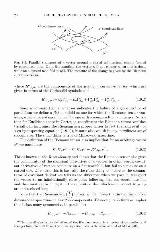
26 BRIEF REVIEW OF GENERAL RELATIVITY
x1 coordinate lines x2 coordinate lines
dx1
dx2
Fig. 1.3: Parallel transport of a vector around a closed infinitesimal circuit formedby coordinate lines. On a flat manifold the vector will not change when this is done,while on a curved manifold it will. The measure of the change is given by the Riemanncurvature tensor.
where Rαβµν are the components of the Riemann curvature tensor, which are
given in terms of the Christoffel symbols as10
Rαβµν := ∂µΓα
βν − ∂νΓαβµ + Γα
ρµΓρβν − Γα
ρνΓρβµ . (1.9.2)
Since a non-zero Riemann tensor indicates the failure of a global notion ofparallelism we define a flat manifold as one for which the Riemann tensor van-ishes, while a curved manifold will be one with a non-zero Riemann tensor. Noticethat for Euclidean space in Cartesian coordinates the Riemann tensor vanishestrivially. In fact, since the Riemann is a proper tensor (a fact that can easily beseen by inspecting equation (1.9.1)), it must also vanish in any curvilinear set ofcoordinates. The same thing is true of Minkowski spacetime.
The definition of the Riemann tensor also implies that for an arbitrary vectorvµ we must have
∇µ∇νvα −∇ν∇µvα = Rαβµνvβ . (1.9.3)
This is known as the Ricci identity and shows that the Riemann tensor also givesthe commutator of the covariant derivatives of a vector. In other words, covari-ant derivatives of vectors commute on a flat manifold, but fail to commute on acurved one. Of course, this is basically the same thing as before as the commu-tator of covariant derivatives tells us the difference when we parallel transportthe vector to an infinitesimally close point following first one coordinate lineand then another, or doing it in the opposite order, which is equivalent to goingaround a closed loop.
Note that the Riemann is a„
13
«tensor, which means that in the case of four
dimensional spacetime it has 256 components. However, its definition impliesthat it has many symmetries, in particular:
Rαβµν = −Rβαµν = −Rαβνµ = Rµναβ , (1.9.4)
10The overall sign in the definition of the Riemann tensor is a matter of convention andchanges from one text to another. The sign used here is the same as that of MTW [206].
1.9 CURVATURE 27
that is, the fully co-variant Riemann tensor is antisymmetric on the first andsecond pair of indices, and symmetric with respect to exchange of these twopairs. Also, it obeys a cyclic relation on the last three indices of the form
Rαβµν + Rα
µνβ + Rανβµ = 0 . (1.9.5)
Using the anti-symmetry with respect to exchange of the last two indices, wefind that this cyclic relation can also be expressed as
Rα[βµν] = 0 , (1.9.6)
so the completely antisymmetric part of Riemann with respect to the last threeindices vanishes.
The symmetries of the Riemann tensor imply that in the end it has onlyn2(n2 − 1)/12 independent components in n dimensions, that is 20 independentcomponents in four dimensions. These symmetries also imply that the trace (i.e.the contraction) of the Riemann tensor over its first and last pairs of indicesvanishes. On the other hand, the trace over the first and third indices does notvanish and is used to define the Ricci curvature tensor:
Rµν := Rλµλν . (1.9.7)
The Ricci tensor is clearly symmetric in its two indices, and in four dimensionshas 10 independent components. Notice that in four dimensions having the Riccitensor vanish does not mean that the manifold is flat, as the remaining 10 com-ponents of Riemann can still be different from zero. However, in three dimensionsit does happen that the vanishing of the Ricci tensor implies that the Riemannis zero, as in that case both these tensors have only six independent componentsand Riemann turns out to be given directly in terms of the Ricci tensor.
Finally, the Ricci scalar, also known as the scalar curvature, is defined as thetrace of the Ricci tensor itself
R := Rµµ . (1.9.8)
An important result regarding the form of the metric and the Christoffelsymbols is the fact that any differentiable manifold with a metric is locally flatin the sense that at any given point on the manifold we can always find a setof coordinates such that the metric tensor becomes diagonal with ±1 elements,and all the Christoffel symbols vanish at that point. This means that we canalways choose orthogonal coordinates at the given point p and guarantee thatsuch coordinates will remain orthogonal in the immediate vicinity of that pointso that ∂µgαβ|p = 0. What we can not do is guarantee that all second derivativesof the metric will vanish because there are in general fewer third derivatives of thecoordinate transformation that can be freely specified than second derivatives ofthe metric tensor itself. In four dimensions, for example, we have 80 independentthird derivatives of the coordinate transformation ∂µ∂ν∂σxα, while there are

28 BRIEF REVIEW OF GENERAL RELATIVITY
100 second derivatives of the metric ∂α∂βgµν that we would need to cancel.This leaves 20 degrees of freedom in the second derivatives of the metric whichcorrespond precisely with the 20 independent components of the Riemann tensor.
1.10 Bianchi identities and the Einstein tensor
Starting from the definition of the Riemann tensor it is possible to show thatthe covariant derivatives of this tensor have the following important property:
Rαβµν;λ + Rα
βλµ;ν + Rαβνλ;µ = 0 , (1.10.1)
or equivalentlyRα
β[µν;λ] = 0 . (1.10.2)
These relations are known as the Bianchi identities, and play a very importantrole in general relativity. One of their most important consequences comes fromcontracting them twice, which results in
Gµν;ν = 0 , (1.10.3)
where Gµν is the so-called Einstein tensor defined as
Gµν := Rµν − 12
gµνR . (1.10.4)
Because of its property of having zero divergence, the Einstein tensor playsa crucial role in the field equations of general relativity, as we will see below.
1.11 General relativity
As already mentioned, the equivalence principle led Einstein to the idea thatgravity could be identified with the curvature of spacetime. This principle saysthat all objects fall with the same acceleration in a gravitational field, some-thing that in the Newtonian theory arises from the fact that the inertial andgravitational masses of a given object are the same. Einstein’s key insight wasto realize that the equivalence principle implies that in a freely falling referenceframe the gravitational force effectively vanishes and the laws of physics lookjust like they do in special relativity. In other words, the equivalence princi-ple implies that there exist local inertial frames, namely those that are fallingfreely. In the presence of a non-uniform gravitational field, however, these localinertial frames can not be glued together to form a global inertial frame, sincefreely falling frames at different locations have accelerations that differ in bothmagnitude and direction.
But the fact that we have local inertial frames can be described geometricallyby saying that locally the spacetime metric is that of Minkowski, and the factthat no global inertial frame exists will correspond to saying that there is no setof coordinates in which the spacetime metric has this simple form everywhere.In other words, spacetime must be a curved manifold, and freely falling frames

1.11 GENERAL RELATIVITY 29
must correspond to locally flat coordinates on that manifold. This remarkableinsight forms the basis of the whole theory of general relativity, which takes as itsbasic postulate the following: Spacetime is a four-dimensional curved manifoldwith a Lorentzian metric.
General relativity therefore generalizes special relativity by considering thepossibility of having a curved spacetime with no global inertial frames. Since noglobal inertial frame exists there is also no natural set of coordinates, so from thestart we must be ready to work on a completely arbitrary coordinate system. Thename “general relativity” comes precisely from the fact that we can use a generalcoordinate system. However, the crucial point is that curvature is allowed, theuse of a general coordinate system in Minkowski spacetime is still only specialrelativity.
Of course, saying that spacetime is curved does not take us too far – one mustsay how to generalize the laws of physics to such a curved spacetime, in particularthe laws of motion of test particles, and also we must say how this curvaturearises in the first place. The second issue is related to the field equations, whichwe will consider in Section 1.13 below; here we will concentrate on the first issue:What are the laws of physics on a curved spacetime?
The first point to stress is the fact that, in general relativity, the gravitationalfield will not correspond to the gravitational force of Newton, as the equivalenceprinciple tells us that such force vanishes in a freely falling frame, i.e. it is justan inertial force analogous to the centrifugal force on a rotating frame. Whatdoes not vanish, even in a freely falling frame, are the tidal forces arising fromthe fact that the gravitational field is not uniform. It is these tidal forces thatare associated with the curvature of spacetime. The laws of physics in generalrelativity come from two basic postulates: the principle of general covariancethat states that these laws must be written in tensor form, and the strong equiv-alence principle that states that in a freely falling frame they must reduce to theform that they have in special relativity. These postulates are not always com-pletely unambiguous, but they work well in most cases and provide us with thesimplest possible generalizations of the laws of physics to a curved background.In particular, these two principles suggest the rule of minimal coupling, whichbasically says that once we have a law of physics that we know holds in specialrelativity, we can generalize it to a curved spacetime by replacing the Minkowskimetric ηαβ for a general metric gαβ, and at the same time replacing all partialderivatives ∂µ for covariant derivatives ∇µ, that is, there should be no explicitcouplings to the curvature. Of course, in all cases, experiments should say if thegeneralizations obtained from these postulates are indeed the correct laws.
A first example of these principles in action corresponds to the motion of afree particle in a curved background. Since in a freely falling frame the particlemust move as it does in special relativity, i.e. in a straight line, in the curvedspacetime it must move following a geodesic. This means that in a gravitationalfield Newton’s first law becomes: A free particle in a curved spacetime movesfollowing timelike geodesics, and light rays move following null geodesics. But
30 BRIEF REVIEW OF GENERAL RELATIVITY
notice that the geodesics of a curved spacetime need not look straight whenprojected into three-dimensional space. Notice also that gravity is not considereda force here – a particle in the presence of a gravitational field with no otherforces acting on it is considered free. This simple law is enough to describe themotion of the planets around the Sun, for example.
It is usual to parameterize a geodesic using the particle’s own proper time τ ,so the equation of motion for a free particle in spacetime takes the form11
d2xα
dτ2+ Γα
βγ
dxβ
dτ
dxγ
dτ= 0 . (1.11.1)
The geodesic equation of motion can also be written as
uµ∇µuα = 0 , (1.11.2)
where u is just the tangent vector to the geodesic curve: uα = dxα/dτ . This vectoris know as the 4-velocity of the particle, and is the relativistic generalization ofthe Newtonian concept of velocity. It is important to notice that
u2 = u · u = gαβdxα
dτ
dxβ
dτ=
ds2
dτ2= −1 , (1.11.3)
that is, the 4-velocity is a unit timelike vector. In an analogous way to Newtonianphysics, the 4-momentum is defined simply as the vector
p := mu , (1.11.4)
where m is the rest mass of the particle.The energy of a particle with 4-momentum p, as measured by an observer
moving with 4-velocity v that has the same position as the particle, is defined interms of the 4-momentum as12
E := −v · p = −vαpα . (1.11.5)
In the particular case when the observer is static in a given coordinate systemits 4-velocity will have components vα = (1/
√−g00, 0, 0, 0), which is easy to seefrom the fact that we must have v · v = −1, so that for this static observerE = p0/
√−g00. In special relativity this reduces to E = mγ, with γ the Lorentzfactor associated with the motion of the particle (or, in SI units, E = mγc2).Notice that since on a curved spacetime there is no global notion of parallelismand no preferred family of observers, in general a given observer can only definean energy for a particle at his own location but not for a particle far away. In
11Of course, this doesn’t work for a light ray for which proper time is always zero, so in thecase of a null geodesic we simply use an arbitrary affine parameter.
12The minus sign in this definition comes from the Lorentzian nature of the metric thatimplies that the time components of co-variant vectors have the opposite sign to what onewould expect.

1.11 GENERAL RELATIVITY 31
special relativity, however, given a specific inertial frame such a preferred familyof observers does exist, and the energy of a particle on that inertial frame cantherefore be globally defined.
There are, however, some special situations when one can define a usefulnotion of energy and other conserved quantities in a global sense on a curvedmanifold. Let us assume that we have a manifold with some symmetry. As wehave seen, associated with that symmetry there will be a Killing vector satisfyingequation (1.8.18). If we now take u to be the 4-velocity of a free particle, or moregenerally the tangent vector to a geodesic curve, we will have
uµ∇µ
(ξ · u
)= uµ∇µ (ξνuν) = ξνuµ∇µuν + uνuµ∇µξν = uµuν∇µξν , (1.11.6)
where we have used the fact that the curve is a geodesic. If we now notice thatthe Killing equation implies that ∇µξν is antisymmetric so that uµuν∇µξν = 0,we finally find
uµ∇µ
(ξ · u
)= 0 . (1.11.7)
This equation implies that if a Killing field ξ exists, then the scalar quantity ξ ·uis constant along the geodesic, so it represents a conserved quantity associatedwith the motion of the particle.
In particular, assume that we have a Killing field that is everywhere timelike.In such a case the spacetime is said to be static, as we can always choose coordi-nates adapted to the Killing field for which the metric coefficients gαβ will be timeindependent. In such adapted coordinates the Killing vector field will have com-ponents ξ = (1, 0, 0, 0), so the above result implies that on a static spacetime thequantity ξ · u = gµνξµuν = g0νuν = u0 is constant along a particle’s trajectory.This means that the co-variant time component of the 4-momentum p0 = mu0is conserved in a static gravitational field and can therefore be defined as thetotal energy of the particle E := −p0. Notice that, in general, this quantity willnot only include the kinetic energy, but will also include contributions from therelativistic equivalent of the gravitational potential energy (as clearly the kineticenergy alone will not be conserved in a gravitational field).13 If the spacetime isnot static, however, this notion of conserved energy is lost.
There are other conserved quantities associated with different symmetries.For example, on a spacetime that has axial symmetry we will find a conservedquantity that can be associated with the angular momentum of the particle.
13One might find confusing the fact that the conserved energy on a static spacetime isE = −p0, while the energy measured locally by a static observer is instead E = −p0/
√−g00.The reason for the difference is that the energy measured locally only corresponds to kineticplus rest mass energy without the potential energy contribution. This can be seen more clearlyin the case of weak gravitational fields and small velocities (see Section 1.14 below), for whichg00 −1− 2φ, with φ 1 the Newtonian potential, and where we find E m + mv2/2 + mφand E = E/
√−g00 m + mv2/2 (neglecting contributions quadratic in φ and v).
32 BRIEF REVIEW OF GENERAL RELATIVITY
1.12 Matter and the stress-energy tensor
In the Newtonian theory, the source of the gravitational field is given by themass density. The equivalence of mass and energy means that we should expectthe energy density to be the source of the gravitational field in general relativity.The first problem we have to deal with, however, is the fact that the energydensity is not a scalar quantity. This is easy to see from the fact that the Lorentztransformations imply that the volume itself is not scalar, and also from thefact that the energy of a particle is a component of the 4-momentum. In fact,it is not difficult to show that the energy density must be a component of arank 2 tensor that includes as its other components the momentum densityand the fluxes of energy and momentum. This tensor is called the stress-energytensor (or sometimes the energy-momentum tensor), and is denoted by T αβ. Thecomponents of this tensor have the following physical interpretations:
T 00 = energy density , (1.12.1)T 0i = momentum density , (1.12.2)T ij = flux of i momentum in direction j. (1.12.3)
The stress-energy tensor can be shown to be symmetric in the general case (forexample, momentum density and energy flux are physically the same thing).Notice that this tensor can be defined for any continuous distribution of matteror energy, that is, it can be defined not only for matter, but also for fields otherthan gravity itself such as the electromagnetic field. Because of this, in generalrelativity it has become customary to simply call matter any type of field thathas a stress-energy tensor associated with it.
Consider now the case of a perfect fluid, that is, a fluid with zero viscosityand zero heat conduction. Such a fluid is characterized by the energy density ρand pressure p as measured by an observer co-moving with the fluid elements,and also by the 4-velocity field u of the fluid elements themselves. In such a case,the stress-energy tensor takes the particularly simple form
T αβ = (ρ + p)uαuβ + p gαβ . (1.12.4)
This expression can be easily derived by noticing that in the Lorentz frame co-moving with the fluid it implies T 00 = ρ, T ii = p and T αβ = 0 for α = β, whichcorresponds to a fluid with energy density ρ, pressure p, zero viscosity (T ij = 0for i = j), and zero heat conduction (T 0i = 0). Equation (1.12.4) is just the fullycovariant expression for such a tensor.
The stress-energy tensor also allows us to write the differential form of thelaws of conservation of energy and momentum in a simple way. The conservationlaw for energy in differential form, for example, states that the change in timeof the energy density inside a small volume element must be balanced by thedifference between the energy that enters the volume element and the energythat leaves (energy is not created or destroyed). In other words, in locally flatcoordinates we should have a continuity equation of the form
1.12 MATTER AND THE STRESS-ENERGY TENSOR 33
∂tT00 + ∂iT
0i = 0 .
The covariant generalization of this conservation law is clearly
∇βT αβ = 0 . (1.12.5)
Notice that this equation includes the conservation of energy for α = 0, andthe conservation of momentum for α = i. This conservation law for energy andmomentum is a fundamental requirement of any physical theory, so we mustdemand the stress-energy tensor of any matter field to satisfy it. As we will seebelow, it also plays a crucial role in the field equations of general relativity.
There is another important comment to be made about equation (1.12.5).Strictly speaking this equation only leads to true conservation of energy, in thesense that the change of energy in a finite region equals the integrated flux ofenergy into that region, when we have a flat spacetime. For a curved spacetimestrict conservation no longer holds as the gravitational field can do work andchange the energy and momentum of the matter (the conservation law (1.12.5)actually represents local conservation as seen by freely falling observers). Wemight think that the obvious thing to do would be to include the stress-energytensor for the gravitational field itself in order to recover full conservation ofenergy, but it turns out that in general relativity no local expression for theenergy of the gravitational field exists.
The conservation laws can in fact also be derived from a variational principle.This can be done in the case when we have a matter field that can be specified bya Lagrangian, that is a scalar function L that depends only on the field variables,their derivatives, and the metric coefficients. Assume that our system is describedby a series of field variables φa, where here a is just a label that numbers thedifferent fields, and not a spacetime index. The Lagrangian will then be a scalarfunction such that L = L(φa, ∂αφa, gαβ). We define the action as the integral ofthe Lagrangian over an (open) region Ω of our manifold
S (Ω) =∫Ω
L dV , (1.12.6)
with dV =√|g| dnx the volume element. We then assume that the dynami-
cal equations are obtained from a least action variational principle, that is, wedemand that the action is stationary with respect to variation in the fields. No-tice, in particular, that the metric gαβ must be considered a dynamical fieldin this variation. Variation with respect to the field variables φa will give usthe so-called field equations, that is the dynamical equations for the field underconsideration, while variation with respect to the metric gives us an equationthat represents the equilibrium between the geometry and the fields, or in otherwords, the conservation laws.
34 BRIEF REVIEW OF GENERAL RELATIVITY
Consider then a variation of the action with respect to the geometry:
δgS = δg
∫Ω
L dV
=∫Ω
[√|g| ∂L
∂gαβδgαβ + L δ
(√|g|)]
dnx
=∫Ω
[√|g| ∂L
∂gαβδgαβ +
12√|g| L δ|g|
]dnx . (1.12.7)
A general result from linear algebra tells us that δ|g| = |g| gαβ δgαβ, so the lastequation can be rewritten as
δgS =∫Ω
T αβδgαβ dV , (1.12.8)
where we have defined the stress-energy tensor as
T αβ :=∂L
∂gαβ+
gαβ
2L
= −gαµgβν ∂L
∂gµν+
gαβ
2L . (1.12.9)
It is usually more convenient to rewrite this definition of the stress-energy tensorin terms of its co-variant components. The expression then becomes
Tαβ := − ∂L
∂gαβ+
gαβ
2L . (1.12.10)
Asking now for the action to be stationary with respect to the variation, i.e. ask-ing for δgS = 0, can be shown to directly imply the conservation laws (1.12.5).14
There is an important comment to be made here. Instead of working with theLagrangian L as the basic dynamical function, we might choose to absorb thevolume element and work with the Lagrangian density L :=
√|g| L. In termsof the Lagrangian density the expression for the stress-energy tensor is morecompact, and takes the simple form:
Tαβ = − 1√|g|∂L
∂gαβ. (1.12.11)
Both expressions for Tαβ are entirely equivalent, but in practice it is faster andmore transparent to use equation (1.12.10) directly to find the stress-energytensor of a field for which we have a Lagrangian L.
14The proof of this involves assuming that the field equations are satisfied, and then consid-ering an arbitrary change of coordinates inside the region Ω. By making use of the fact thatthis change of coordinates can not affect the action integral, and looking at the change in theform of the integrand itself, the conservation laws follow.

1.12 MATTER AND THE STRESS-ENERGY TENSOR 35
Consider, for example, a Klein–Gordon field φ with mass m, also known asa scalar field. Its Lagrangian is given by
L = − (∇αφ∇αφ + m2φ2)
= − (gαβ∇αφ ∇βφ + m2φ2)
. (1.12.12)
Using (1.12.10) we find immediately that the corresponding stress-energy tensorhas the form
Tαβ = ∇αφ ∇βφ − gαβ
2(∇µφ∇µφ + m2φ2
). (1.12.13)
Fundamental scalar fields are not known to exist in nature. Still, the simplicity oftheir stress-energy tensor and dynamical equation (see below) means that theyare an ideal test system for studying properties of solutions to the field equa-tions of general relativity, and because of this they are often used in numericalrelativity. Also, fundamental theories of particle physics demand the existenceof scalar fields, an example of this is the Higgs field of the standard model.
Consider now the case of an electromagnetic field described by the potential4-vector A := (ϕ, Ai), with ϕ the scalar potential and Ai the vector potential (butnotice that in tensorial terms neither ϕ is a scalar nor Ai a vector; they are infact different components of the same 4-vector). Define now the electromagneticfield as the following antisymmetric tensor
Fαβ = 2 ∇[αAβ] . (1.12.14)
The electric field E and magnetic field B are then defined through
Fαβ =
⎛⎜⎜⎝0 Ex Ey Ez
−Ex 0 Bz −By
−Ey −Bz 0 Bx
−Ez By −Bx 0
⎞⎟⎟⎠ . (1.12.15)
This shows that the electric and magnetic fields are in fact not two separate3-vectors, but rather the six independent components of an antisymmetric rank2 tensor. In particular, under Lorentz transformations the components of theelectric and magnetic fields mix together. The Lagrangian for the electromagneticfield turns out to be
L = − 18π
FαβFαβ = − 18π
gαµgβνFµνFαβ , (1.12.16)
which is not surprising since, apart from normalization factors, it is the onlyscalar we can form that is quadratic in the field. From this Lagrangian we findthe following stress-energy tensor:
Tαβ =14π
(FαµFβ
µ − gαβ
4FµνFµν
). (1.12.17)
We can readily verify that this gives the standard expressions for the energydensity and momentum density (Poynting vector) for the electromagnetic field.

36 BRIEF REVIEW OF GENERAL RELATIVITY
A Lagrangian can in fact also be defined for a perfect fluid, but the derivationof the corresponding stress-energy tensor from such a Lagrangian is considerablyless transparent than in the cases of the Klein-Gordon and electromagnetic fields,so we will not consider it here.
The conservation laws (1.12.5) are often enough to find the dynamical equa-tions for the system under consideration. For example, in the case of a perfectfluid they reduce to the first law of thermodynamics (conservation of energy)and the relativistic Euler equations (conservation of momentum). In the case ofa scalar field, the conservation laws imply directly the Klein–Gordon equation:
φ − m2φ = 0 , (1.12.18)
where := gµν∇µ∇ν is the d’Alambertian operator.
1.13 The Einstein field equationsOnce we know how to generalize the laws of physics to curved spacetimes, thefinal building block still missing from the theory of general relativity is the onethat relates the geometry of spacetime with the distribution of mass and en-ergy. This last element is contained in the Einstein field equations, or simplyEinstein’s equations. These equations can be derived in several different ways,either looking for a consistent relativistic generalization of Newton’s theory (theroad followed by Einstein), or deriving them in a formal way from a variationalprinciple starting with an adequate Lagrangian (the road followed by Hilbert).
The more intuitive way to derive these equations is to go back for a while toNewton’s theory of gravity. Assume we have a Newtonian gravitational potentialφ. The gravitational force will be given by dv/dt = −∇φ.15 In general relativity,on the other hand, the motion of free particles is described by the geodesicequation, which can be written in the form
duα
dτ= −Γα
µν
duµ
dτ
duν
dτ. (1.13.1)
From this it is clear that the Christoffel symbols play the role of ∇φ, so themetric coefficients must play the role of the potential φ. However, as mentionedbefore, the metric and Christoffel symbols are not the best way to describe thecurvature of spacetime since they can be made to become trivial by choosinglocally flat coordinates, which physically means going to a freely falling framewhere the gravitational force vanishes. We should then concentrate on the tidalforces which carry the real physical information about the gravitational field.
In Newton’s theory, the tidal acceleration between two nearby freely fallingparticles with separation z = x2 − x1 is given by d2z/dt2 = −(z · ∇) ∇φ. In gen-eral relativity the tidal acceleration will correspond to the acceleration between
15One should not be confused with the use of the ∇ symbol here. When referring to Newton’stheory this symbol should be understood to mean just the standard three-dimensional gradient,and not a covariant derivative.
1.13 THE EINSTEIN FIELD EQUATIONS 37
nearby geodesics, also known as geodesic deviation. Consider a congruence ofgeodesics with tangent vector uα and parameter λ, and define the separation be-tween two nearby geodesics as zα(λ) = xα
1 (λ) − xα2 (λ). The tidal acceleration will
then be given by aα := uµ∇µ(uν∇νzα). We can show that this tidal accelerationis given in terms of the Riemann curvature tensor as:
aα = −Rαµβνuµuνzβ . (1.13.2)
We then see that, in flat space, geodesics do not deviate from each other, or inother words parallel straight lines remain parallel (which is Euclid’s famous fifthpostulate). In a curved space, however, geodesic lines deviate from each other.
Comparing the Newtonian and relativistic expressions for the tidal accel-eration we see that Rα
µβνuµuν plays the role of ∂i∂jφ. On the other hand,the energy density measured by an observer following the geodesic is given byρ = Tµνuµuν , which suggests that the relativistic version of Newton’s field equa-tion ∇2φ = 4πρ should have the form Rα
µανuµuν = 4πTµνuµuν , and since thevector uα is arbitrary this reduces to Rµν = 4πTµν . The last equation has thestructure we would expect, as it relates second derivatives of the metric (thegravitational “potential”) with the energy density, just as in Newton’s theory.This field equation was in fact considered by Einstein, but he quickly realizedthat it can’t be correct since the conservation laws ∇µT µν = 0 would imply that∇µRµν = 0, which imposes a serious restriction in the allowed geometries ofspacetime.
The solution to the problem of the compatibility of the field equations andthe conservation laws comes from considering the contracted Bianchi identities.In particular, these identities imply that the Einstein tensor (1.10.4) has zerodivergence, so a consistent version of the field equations would be
Gµν ≡ Rµν − 12
gµνR = 8πTµν , (1.13.3)
where the factor of 8π is there in order to recover the correct Newtonian limit.These are the field equations of general relativity, or in short Einstein’s equations.Note that they are in fact ten equations, as the indices µ and ν take values from0 to 3, and both the Einstein and stress-energy tensors are symmetric. Noticealso that, as written above, the field equations imply the conservation laws, as∇µT µν = 0 follows from pure geometric consistency.
It is sometimes useful to rewrite the field equations in the equivalent form
Rµν = 8π
(Tµν − 1
2gµνT
), (1.13.4)
with T := T µµ the trace of the stress-energy tensor. This equation can be ob-
tained by simply taking the trace of the original field equations and noticingthat they imply R = −8πT (the trace of the metric is always equal to the totalnumber of dimensions of the manifold, which in the case of spacetime is 4).
38 BRIEF REVIEW OF GENERAL RELATIVITY
The Einstein equations just introduced could not appear to be more simple.This simplicity, however, is only apparent since each term is a short-hand forconsiderably more complex objects. Written in their most general form, in anarbitrary coordinate system and with all terms expanded out, the Einstein equa-tions become a system of ten coupled, non-linear, second order partial differentialequations with thousands of terms.
In the case of vacuum the stress-energy tensor vanishes, and Einstein’s equa-tions reduce to:
Gµν = 0 , (1.13.5)
or equivalently,Rµν = 0 . (1.13.6)
Note that, as mentioned before, the fact that the Ricci tensor vanishes does notimply that spacetime is flat. This is as it should be, since we know that thegravitational field of an object extends beyond the object itself, which meansthat the curvature of spacetime in the empty space around a massive objectcan not be zero. The Einstein equations in vacuum have another importantconsequence, they describe the way in which the gravitational field propagates inempty space and, in an analogous way to electromagnetism, predict the existenceof gravitational waves: perturbations in the gravitational field that propagate atthe speed of light. The prediction of the existence of gravitational waves tellsus that, in Einstein’s theory, gravitational interactions do not propagate at aninfinite speed, but rather at the speed of light (see Section 1.14 below).
The field equations (1.13.3) can also be derived from a variational principle,we only need to introduce a Lagrangian for the gravitational field itself. Sincegravity is associated with the Riemann tensor, and the Lagrangian must be ascalar, the only possibility is to take the Ricci scalar as the Lagrangian:
LG = R . (1.13.7)
If we now consider the total Lagrangian to be L = LG + LM , with LM theLagrangian associated with the matter, and ask for the action integral to bestationary, Einstein’s field equations follow. This was the approach followed byD. Hilbert, who derived the field equations independently of Einstein (in fact,Hilbert’s derivation came first by a few days). Because of this the field equationsare also known as the Einstein–Hilbert equations.
There are two important final comments to be made about the Einstein fieldequations. The first has to do with the relation between the field equations andthe conservation laws. Since the conservation laws are a consequence of the fieldequations, and they in turn contain all the dynamical information in many cases,it turns out that often we do not need to postulate the equations of motion for thematter as they can be derived directly from the field equations. In particular, for

1.14 WEAK FIELDS AND GRAVITATIONAL WAVES 39
a perfect fluid with zero pressure (known as dust in relativity), the field equationspredict that the flow lines should be timelike geodesics. Also, it can be shownthat a small test body with weak self-gravity will necessarily move on a geodesic.So there is really no need to postulate geodesic motion of test particles in generalrelativity – it is a consequence of the field equations.
The second comment has to do with the meaning of a solution to the Ein-stein equations. Notice that we have ten second-order differential equations forthe ten components of the metric tensor gµν , so naively we might expect that,given a matter distribution and appropriate boundary conditions, the full met-ric tensor would be completely determined. But this can not be since the gµν
are components of a tensor in some specific coordinate system. If we changethe coordinates the components of the metric tensor will change, but the phys-ical content of the solution can not depend on the choice of coordinates. Thismeans that a “solution” of the field equations should really be understood asthe equivalence class of all four-dimensional metrics related to each other by achange of coordinates. Since there are four coordinates, there are four arbitrarydegrees of freedom in the metric components, so the field equations should onlyfix the remaining six components. But this is precisely the content of the Bianchiidentities ∇νGµν = 0 – they provide us with four differential relations betweenthe ten field equations, so there are in fact only six independent equations. Ingeneral there is no “natural” way of separating the six independent componentsof gµν in a clear way. However, such a separation can be achieved by choosing aspecific set of coordinates such as the one used in the 3+1 formulation that wewill study in Chapter 2.
1.14 Weak fields and gravitational wavesNewton’s theory served well for over two centuries. The reason is that the grav-itational fields on the Solar System, including that of the Sun, are actually veryweak. In fact, Einstein’s motivation for developing general relativity was purelytheoretical, as at the time there were no strong observational reasons to aban-don Newton’s theory (the advance of Mercury’s perihelion was known, but itwas a very small effect and at the time there was still hope that some unknownNewtonian perturbation could account for it). The study of weak gravitationalfields is therefore very important, not only because they correspond to a verycommon case, but also because they lead to the prediction of the existence ofgravitational radiation.
Since in general relativity the gravitational field is associated with the curva-ture of spacetime, weak gravitational fields will correspond to nearly flat space-times. In such a case there must exist coordinates such that the metric tensor isnearly that of Minkowski, that is
gµν = ηµν + hµν , |hµν | 1 . (1.14.1)
Notice that here we are assuming not only that the curvature is small, but alsothat our spatial coordinates are nearly Cartesian.
40 BRIEF REVIEW OF GENERAL RELATIVITY
An interesting observation arises from considering what is known as a back-ground Lorentz transformation. If we transform our nearly flat coordinates usingthe Lorentz transformations (1.3.2) we find that
gµν = ΛαµΛβ
ν gαβ = ΛαµΛβ
ν (ηαβ + hαβ)
= ηµν + ΛαµΛβ
νhαβ = ηµν + hµν , (1.14.2)
where we have defined hµν := ΛαµΛβ
νhαβ . We then see that hµν transforms justas it would if it were a rank 2 tensor in special relativity. This implies thatwe can reinterpret a weak gravitational field as just a field in special relativityassociated with a symmetric rank 2 tensor hµν . We can then work as if we hada flat spacetime with a tensor field hµν defined on it, and use the Minkowskimetric to raise and lower indices of tensors. The only exception to the rule ofusing ηµν to move indices around will be the metric tensor gµν itself. Since gµν
is by definition the inverse matrix to gµν , to first order in hµν we must have
gµν = ηµν − hµν . (1.14.3)
The linearized field equations are now easy to derive. We can show that tolinear order in hµν the Riemann tensor turns out to be
Rαβµν =12
(∂β∂µhαν + ∂α∂νhβµ − ∂β∂νhαµ − ∂α∂µhβν) , (1.14.4)
and the Ricci tensor becomes
Rµν = ∂α∂(µhν)α − 12
(∂µ∂νh + ∂α∂αhµν) , (1.14.5)
with h := hαα the trace of hµν , and ∂α ≡ ηαβ∂β . If we define the trace reversed
field tensor hµν := hµν − ηµνh/2, the Einstein tensor turns out to be
Gµν = ∂α∂(µhν)α − 12(∂α∂αhµν + ηµν∂α∂βhαβ
), (1.14.6)
and the linearized field equations become
∂α∂(µhν)α − 12(∂α∂αhµν + ηµν∂α∂β hαβ
)= 8πTµν . (1.14.7)
These equations, however, are still more complicated than they need to be.In order to simplify them further, consider for a moment a small, but arbitrary,change of coordinates of the form xµ = xµ + ξµ, where ξ is a small vector in thesense that |∂νξµ| 1. The Jacobian matrix will then be given by
Λµν = ∂νxµ = δµ
ν + ∂νξµ , (1.14.8)
and the inverse transformation will be (to first order)
1.14 WEAK FIELDS AND GRAVITATIONAL WAVES 41
Λνµ = δν
µ − ∂µξν . (1.14.9)
The transformation of the metric is gµν = ΛαµΛβ
ν gαβ, which to first order becomes
gµν = ηµν + hµν − 2∂(µξν) . (1.14.10)
Since this is only a coordinate transformation, we find that a transformationof the metric of this type leaves the physical situation intact for arbitrary (butstill small) ξα. This is called a gauge transformation, and we say that linearizedgravity has a gauge freedom of the form
hµν → hµν − 2∂(µξν) , (1.14.11)
or in terms of hµν :hµν → hµν − 2∂(µξν) + ηµν∂αξα . (1.14.12)
This is entirely analogous to the electromagnetic case, where we find that theelectromagnetic field Fαβ (and hence the physics) remains unaffected by trans-formations in the potential of the form Aµ → Aµ + ∂µf , for an arbitrary scalarfunction f . In the case of gravity the word gauge is perhaps even more appro-priate as we are in fact dealing with a change in the conventions for measuringdistances, i.e. the coordinates.
We can now use the gauge freedom to simplify the equations by choosing avector ξ that solves the equation
∂α∂αξβ = ∂αhαβ . (1.14.13)
That this equation can always be solved is easy to see from the fact that it isnothing more than the wave equation for ξβ with a source given by ∂αhαβ . If wedo this we find that the gauge transformation implies that
∂ν hνµ → ∂ν hνµ − ∂ν∂νξµ = 0 , (1.14.14)
That is, we can always find a gauge such that hµν has zero divergence. Such agauge is called the Lorentz gauge, a name taken from the analogous condition inelectromagnetism ∂µAµ = 0.
If we assume that we are in the Lorentz gauge we will have
∂ν hνµ = 0 , (1.14.15)
and the field equations (1.14.7) will reduce to
hµν = −16πTµν , (1.14.16)
where now stands for the d’Alambertian operator in flat space, or in otherwords the wave operator. These are the field equations for a weak gravitationalfield in their standard form.

42 BRIEF REVIEW OF GENERAL RELATIVITY
One particularly important application of the weak field approximation is theNewtonian limit of general relativity. Notice that this limit will correspond notonly to weak fields, but also to small velocities of the sources. Small velocitiesimply that the energy density T 00 is much larger than both the momentumdensity and the stresses. In that case we can in fact consider only the componenth00 and ignore all others (h0i hij 0). The field equations then reduce to
h00 = −16πρ . (1.14.17)
Moreover, small velocities also imply that time derivatives in the d’Alambertianoperator are much smaller than spatial derivatives, so the equation simplifies to
∇2h00 = −16πρ , (1.14.18)
where here the symbol ∇2 should be understood as the three-dimensional Laplaceoperator. This approximation implies that the speed of the sources is muchsmaller than the speed of light, so we might take the gravitational field to prop-agate essentially instantaneously. Comparing this with Newton’s field equation∇2φ = 4πρ, we conclude that in this limit h00 = −4φ and h0i = hij = 0. Go-ing back to the definition of hαβ in terms of hαβ , we find that this impliesh00 = hii = −2φ. The spacetime metric in the Newtonian approximation thentakes the final form
ds2 = − (1 + 2φ) dt2 + (1 − 2φ)(dx2 + dy2 + dz2
), (1.14.19)
with φ the standard Newtonian gravitational potential. Notice that in geometricunits φ is dimensionless, and for the weak field approximation to be valid wemust have φ 1, which in fact is always the case for gravitational fields in theSolar System.16One should also stress the fact that, even if in this limit the fieldequation is the same as that of Newton, the Newtonian limit of general relativityis a considerably richer theory as the metric above can be shown to directlyimply the effects of gravitational time dilation and the bending of light rays ina gravitational field, both of which are absent in Newton’s theory.
Another consequence of fundamental importance coming from the weak fieldequations is the existence of gravitational waves. Consider the weak field equa-tions in vacuum, without assuming anything about the sources that might haveproduced that field. The Einstein equations in this case take the form
hµν =(−∂2t + ∇2) hµν = 0 , (1.14.20)
which is nothing more than the wave equation for waves propagating at the speedof light (c = 1). So we find that perturbations in the gravitational field behave
16The Newtonian gravitational field at the surface of the Sun in geometric units is φ ∼ 10−6,while at the surface of the Earth it is φ ∼ 10−9.

1.14 WEAK FIELDS AND GRAVITATIONAL WAVES 43
as waves that propagate at the speed of light, i.e. the field equations predict theexistence of gravitational waves. The simplest solution to the above equation areplane gravitational waves of the form
hµν = Aµν exp (ikαxα) , (1.14.21)
with Aµν the amplitude tensor of the waves and kµ the wave vector. Substitutingthis into the wave equation we immediately find that
ηαβkαkβ = kαkα = 0 , (1.14.22)
that is, the wave vector must be null, which is just another way of saying that thewaves propagate at the speed of light. We must remember, however, that the fieldequations only take the simplified form (1.14.20) in the Lorentz gauge (1.14.15),which in this case implies that
Aαβkβ = 0 , (1.14.23)
that is, the amplitude tensor Aµν must be orthogonal to the wave vector.At this point we might think that gravitational waves have six independent
degrees of freedom: The ten independent components of the symmetric tensorAαβ , minus the four constraints imposing the Aαβ must be orthogonal to kα. Thisis, however, not true since there is still considerable gauge freedom left withinthe Lorentz gauge. The reason is that when we impose the Lorentz gauge bychoosing a specific gauge transformation vector ξα, we are in fact only restrictingthe value of ξα, so we can add to this ξα any new vector ξα such that ξα = 0without changing anything. In particular, we can take ξα = Bα exp(ikβxβ) forany arbitrary constant vector Bα. We then have four extra gauge degrees offreedom, which reduces the independent components of Aµν to only two. In fact,we can always choose a Bα such that two further conditions are imposed on Aµν
Aµµ = 0 , Aµνuν = 0 , (1.14.24)
for an arbitrary constant 4-velocity uα (i.e. an arbitrary timelike unit vector).The first condition means that Aµν is traceless (which implies that in thisgauge hµν = hµν), and the second that it is orthogonal to uµ. If we move to aLorentz frame such that uα = (1, 0, 0, 0), then in that frame conditions (1.14.23)and (1.14.24) imply that
Aµ0 = 0 ,∑
j
Aijkj = 0 ,∑
j
Ajj = 0 . (1.14.25)
Any tensor that satisfies these conditions is called a transverse-traceless (TT)tensor, traceless since its trace clearly vanishes, and transverse because it is bothpurely spatial and orthogonal to its own direction of propagation. If we take the
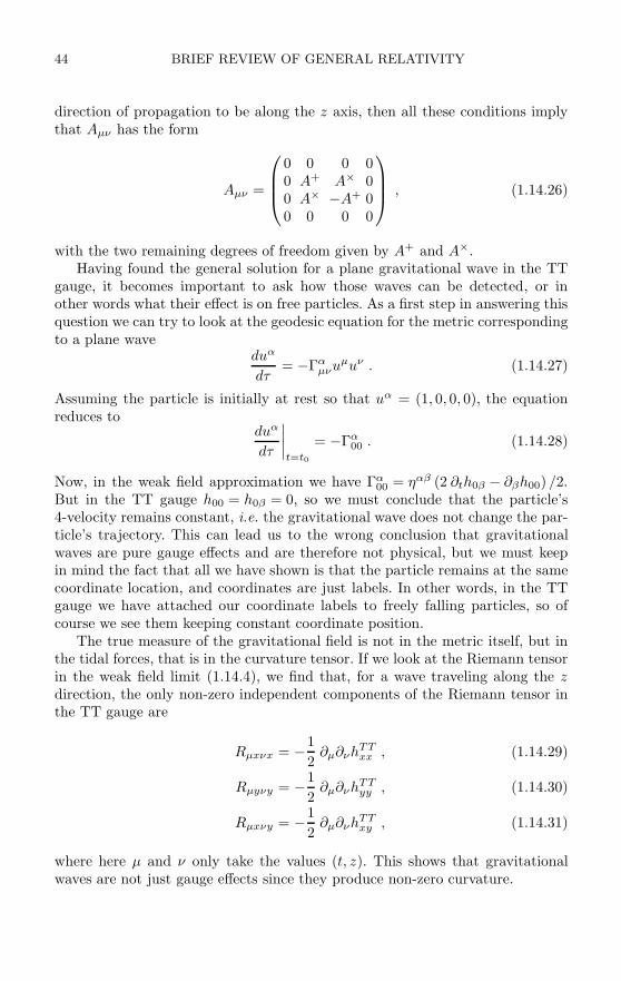
44 BRIEF REVIEW OF GENERAL RELATIVITY
direction of propagation to be along the z axis, then all these conditions implythat Aµν has the form
Aµν =
⎛⎜⎜⎝0 0 0 00 A+ A× 00 A× −A+ 00 0 0 0
⎞⎟⎟⎠ , (1.14.26)
with the two remaining degrees of freedom given by A+ and A×.Having found the general solution for a plane gravitational wave in the TT
gauge, it becomes important to ask how those waves can be detected, or inother words what their effect is on free particles. As a first step in answering thisquestion we can try to look at the geodesic equation for the metric correspondingto a plane wave
duα
dτ= −Γα
µνuµuν . (1.14.27)
Assuming the particle is initially at rest so that uα = (1, 0, 0, 0), the equationreduces to
duα
dτ
∣∣∣∣t=t0
= −Γα00 . (1.14.28)
Now, in the weak field approximation we have Γα00 = ηαβ (2 ∂th0β − ∂βh00) /2.
But in the TT gauge h00 = h0β = 0, so we must conclude that the particle’s4-velocity remains constant, i.e. the gravitational wave does not change the par-ticle’s trajectory. This can lead us to the wrong conclusion that gravitationalwaves are pure gauge effects and are therefore not physical, but we must keepin mind the fact that all we have shown is that the particle remains at the samecoordinate location, and coordinates are just labels. In other words, in the TTgauge we have attached our coordinate labels to freely falling particles, so ofcourse we see them keeping constant coordinate position.
The true measure of the gravitational field is not in the metric itself, but inthe tidal forces, that is in the curvature tensor. If we look at the Riemann tensorin the weak field limit (1.14.4), we find that, for a wave traveling along the zdirection, the only non-zero independent components of the Riemann tensor inthe TT gauge are
Rµxνx = −12
∂µ∂νhTTxx , (1.14.29)
Rµyνy = −12
∂µ∂νhTTyy , (1.14.30)
Rµxνy = −12
∂µ∂νhTTxy , (1.14.31)
where here µ and ν only take the values (t, z). This shows that gravitationalwaves are not just gauge effects since they produce non-zero curvature.
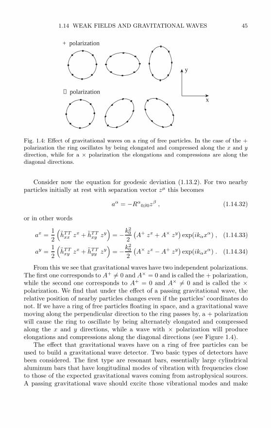
1.14 WEAK FIELDS AND GRAVITATIONAL WAVES 45
+ polarization
× polarizationx
y
Fig. 1.4: Effect of gravitational waves on a ring of free particles. In the case of the +polarization the ring oscillates by being elongated and compressed along the x and ydirection, while for a × polarization the elongations and compressions are along thediagonal directions.
Consider now the equation for geodesic deviation (1.13.2). For two nearbyparticles initially at rest with separation vector zµ this becomes
aα = −Rα0β0z
β , (1.14.32)
or in other words
ax =12
(hTT
xx zx + hTTxy zy
)= −k20
2(A+ zx + A× zy
)exp(ikαxα) , (1.14.33)
ay =12
(hTT
xy zx + hTTyy zy
)= −k20
2(A× zx − A+ zy
)exp(ikαxα) . (1.14.34)
From this we see that gravitational waves have two independent polarizations.The first one corresponds to A+ = 0 and A× = 0 and is called the + polarization,while the second one corresponds to A+ = 0 and A× = 0 and is called the ×polarization. We find that under the effect of a passing gravitational wave, therelative position of nearby particles changes even if the particles’ coordinates donot. If we have a ring of free particles floating in space, and a gravitational wavemoving along the perpendicular direction to the ring passes by, a + polarizationwill cause the ring to oscillate by being alternately elongated and compressedalong the x and y directions, while a wave with × polarization will produceelongations and compressions along the diagonal directions (see Figure 1.4).
The effect that gravitational waves have on a ring of free particles can beused to build a gravitational wave detector. Two basic types of detectors havebeen considered. The first type are resonant bars, essentially large cylindricalaluminum bars that have longitudinal modes of vibration with frequencies closeto those of the expected gravitational waves coming from astrophysical sources.A passing gravitational wave should excite those vibrational modes and make
46 BRIEF REVIEW OF GENERAL RELATIVITY
the bars resonate. The first of these bars were constructed by Joseph Weberin the 1960s, and several modern versions that work at cryogenic temperaturesare still in use today. The second type of detectors are laser interferometers,where we track the separation of freely suspended masses using highly accurateinterferometry. The first prototype interferometers where build in the 1980s,and today several advanced kilometer-scale interferometric detectors are eitheralready working or in the last stages of development: The LIGO project in theUnited States, the VIRGO and GEO 600 projects in Europe, and the TAMAproject in Japan.
To this day, there has been no unambiguous detection of gravitational waves,though this might change in the next few years as the new interferometers slowlyreach their design sensitivities. The main reason why gravitational waves havenot been observed yet has to do with the fact that gravity is by far the weakest ofall known interactions. Estimates of the amplitudes of gravitational waves comingfrom violent astrophysical events such as the collisions of neutron stars or blackholes from distances as far away as the Virgo Cluster put the dimensionlessamplitude of the waves as they reach Earth at the level of A ∼ 10−21. In otherwords, a ring of particles one meter in diameter would be deformed a distanceof roughly one millionth of the size of a proton (the effect scales with the sizeof the system, which explains why the large interferometric detectors have armswith lengths of several kilometers). Detecting such small distortions is clearly ahuge challenge. However, with modern technology such a detection has becomenot only possible but even likely before this decade is out.
The prediction of the gravitational wave signal coming from highly relativisticgravitational systems is one of the most important applications of numericalrelativity, and because of this we will come back to the subject of gravitationalwaves in later Chapters.
1.15 The Schwarzschild solution and black holes
One particularly important application of general relativity is related to theexterior gravitational field of a static and spherically symmetric object. Thegeneral metric of such a spacetime can be shown to have the simple form
ds2 = −f(r)dt2 + h(r)dr2 + R(r)2dΩ2 , (1.15.1)
where r is some radial coordinate, and f , h and R are functions of r only. Wecan simplify this further by choosing a radial coordinate r′ such that r′ := R(r).In that case the metric reduces to
ds2 = −f(r)dt2 + h(r)dr2 + r2dΩ2 , (1.15.2)
where for simplicity we have dropped the prime from r′. In the general case wehave therefore only two unknown functions to determine, f(r) and h(r). Thecoordinates (r, θ, φ) are known as Schwarzschild coordinates, and in particularthe radial coordinate is called the areal radius since in this case the area of the

1.15 THE SCHWARZSCHILD SOLUTION AND BLACK HOLES 47
sphere is always given by 4πr2.17 Equation (1.15.2) for the metric allows fora huge simplification in the field equations: Instead of having to solve for 10independent metric components we only need to find two functions of r.
The next step is to substitute the metric (1.15.2) into the Einstein fieldequations in order to find f and h. Since we are interested in the exterior field,we must use the vacuum field equations Rµν = 0. Doing this we find
0 = Rtt =12(fh)−1/2
d
dr
[(fh)−1/2
df
dr
]+
1rfh
df
dr, (1.15.3)
0 = Rrr = −12(fh)−1/2
d
dr
[(fh)−1/2
df
dr
]+
1rh2
dh
dr, (1.15.4)
0 = Rθθ = Rφφ = − 12rfh
df
dr+
12rh2
dh
dr+
1r2
(1 − 1
h
), (1.15.5)
with all other components of Rµν equal to zero. The first two equations imply
d ln f
dr+
d ln h
dr= 0 , (1.15.6)
which can be trivially integrated to find f = K/h, with K some constant. With-out loss of generality we can take K = 1, as this only requires rescaling the timecoordinate. Substituting this into the third equation we find
−df
dr+
1 − f
r= 0 ⇒ d
dr(rf) = 1 , (1.15.7)
whose solution isf = 1 + C/r , (1.15.8)
with C another constant. The metric then takes the form
ds2 = −(
1 +C
r
)dt2 +
(1 +
C
r
)−1dr2 + r2dΩ2 . (1.15.9)
The value of the constant C can be obtained by comparing with the Newto-nian limit (1.14.19), which should correspond to r >> 1. Taking the Newtonianpotential to be φ = −M/r we find C = −2M , which implies
ds2 = −(
1 − 2M
r
)dt2 +
(1 − 2M
r
)−1dr2 + r2dΩ2 . (1.15.10)
17Notice, however, that there is no reason why the distance to the origin of the coordinatesystem r = 0 should be equal to r. In fact, there is no reason why the point r = 0 should bepart of the manifold at all. For example, consider the geometry of a parabola of revolution.The areal radius in this case will measure the circumference of the surface at a given place,but there is clearly no point with r = 0 on the surface. In fact, the areal radius is not alwayswell behaved. Think of a two-dimensional surface of revolution that resembles a bottle with anarrow throat (this is called a bag of gold geometry). It is clear that as we go from inside thebottle towards the throat and then out of the bottle, the areal radius first becomes smallerand then larger again, i.e. it is not monotone so it is not a good coordinate.
48 BRIEF REVIEW OF GENERAL RELATIVITY
This is known as the Schwarzschild solution, in honor of K. Schwarzschild whodiscovered it in 1916 [260], a few months after Einstein first postulated the fieldequations of general relativity. Among the properties of the previous solution wecan first mention the fact that it is asymptotically flat, that is, it approaches theMinkowski metric when r → ∞. This is to be expected as the gravitational fieldbecomes weaker as we move away from the source. More interesting is the factthat the metric coefficients become singular at both r = 0 and r = 2M . Theradius rs := 2M is known as the Schwarzschild or gravitational radius, and forconventional astrophysical objects (planets, stars, etc.) it is usually much smallerthan the actual radius of the object itself. Since the Schwarzschild solution is avacuum solution it is no longer valid for r smaller than the radius of the object,so in those cases we do not need to worry about the metric singularities.
If, on the other hand, we wish to consider Schwarzschild’s solution as thatcorresponding to a point particle, we must deal with the metric singularities atr = 0 and r = 2M . In order to study the nature of these singularities it isconvenient to first calculate the Riemann tensor for this spacetime. Doing thiswe find that the only non-zero components of Riemann are
Rtrtr = −2M/r3 , (1.15.11)Rtθtθ = Rtφtφ = M/r3 , (1.15.12)
Rθφθφ = 2M/r3 , (1.15.13)Rrθrθ = Rrφrφ = −M/r3 . (1.15.14)
Notice that none of these components are singular at r = 2M , but they are allsingular at r = 0. This means that the gravitational field is singular at r = 0(as we would expect for a point particle), but perfectly regular at r = 2M . Theonly possibility is therefore that at r = 2M something goes wrong with theSchwarzschild coordinates.
There is something else to notice about Schwarzschild’s solution. For r < 2Mit turns out that the coordinates r and t change roles: r becomes a timelikecoordinate (grr < 0), while t becomes spacelike (gtt > 0). This implies that oncean object has crossed r = 2M , the advance of time becomes equivalent with adecrease in r, that is, the object must continue toward smaller values of r forthe same reason that time must flow to the future. As nothing can stop the flowof time, there is no force in the Universe capable of preventing the object fromreaching r = 0, where it will find infinite tidal forces (the Riemann is singular)that will destroy it. The Schwarzschild radius represents a surface of no return:Further out it is always possible to escape the gravitational field, but move closerthan r = 2M and the fall all the way down to r = 0 becomes inevitable.
Since the regularity of Riemann implies that the problem at r = 2M mustbe caused by a poor choice of coordinates, we can ask the question of whetheror not a better set of coordinates exists to study the Schwarzschild spacetime.In fact, we can construct several coordinate systems that are regular at r = 2M .One of the first are the so-called Eddington–Finkelstein coordinates, discovered
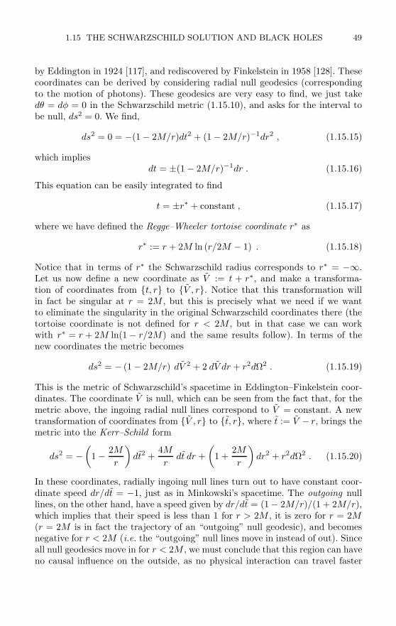
1.15 THE SCHWARZSCHILD SOLUTION AND BLACK HOLES 49
by Eddington in 1924 [117], and rediscovered by Finkelstein in 1958 [128]. Thesecoordinates can be derived by considering radial null geodesics (correspondingto the motion of photons). These geodesics are very easy to find, we just takedθ = dφ = 0 in the Schwarzschild metric (1.15.10), and asks for the interval tobe null, ds2 = 0. We find,
ds2 = 0 = −(1 − 2M/r)dt2 + (1 − 2M/r)−1dr2 , (1.15.15)
which impliesdt = ±(1 − 2M/r)−1dr . (1.15.16)
This equation can be easily integrated to find
t = ±r∗ + constant , (1.15.17)
where we have defined the Regge–Wheeler tortoise coordinate r∗ as
r∗ := r + 2M ln (r/2M − 1) . (1.15.18)
Notice that in terms of r∗ the Schwarzschild radius corresponds to r∗ = −∞.Let us now define a new coordinate as V := t + r∗, and make a transforma-tion of coordinates from t, r to V , r. Notice that this transformation willin fact be singular at r = 2M , but this is precisely what we need if we wantto eliminate the singularity in the original Schwarzschild coordinates there (thetortoise coordinate is not defined for r < 2M , but in that case we can workwith r∗ = r + 2M ln(1 − r/2M) and the same results follow). In terms of thenew coordinates the metric becomes
ds2 = − (1 − 2M/r) dV 2 + 2 dV dr + r2dΩ2 . (1.15.19)
This is the metric of Schwarzschild’s spacetime in Eddington–Finkelstein coor-dinates. The coordinate V is null, which can be seen from the fact that, for themetric above, the ingoing radial null lines correspond to V = constant. A newtransformation of coordinates from V , r to t, r, where t := V − r, brings themetric into the Kerr–Schild form
ds2 = −(
1 − 2M
r
)dt2 +
4M
rdt dr +
(1 +
2M
r
)dr2 + r2dΩ2 . (1.15.20)
In these coordinates, radially ingoing null lines turn out to have constant coor-dinate speed dr/dt = −1, just as in Minkowski’s spacetime. The outgoing nulllines, on the other hand, have a speed given by dr/dt = (1 − 2M/r)/(1 + 2M/r),which implies that their speed is less than 1 for r > 2M , it is zero for r = 2M(r = 2M is in fact the trajectory of an “outgoing” null geodesic), and becomesnegative for r < 2M (i.e. the “outgoing” null lines move in instead of out). Sinceall null geodesics move in for r < 2M , we must conclude that this region can haveno causal influence on the outside, as no physical interaction can travel faster
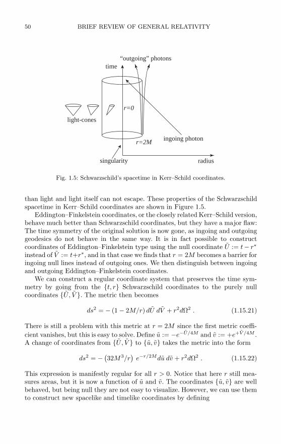
50 BRIEF REVIEW OF GENERAL RELATIVITY
time
r=2M
r=0
ingoing photon
radius
light-cones
“outgoing” photons
singularity
Fig. 1.5: Schwarzschild’s spacetime in Kerr–Schild coordinates.
than light and light itself can not escape. These properties of the Schwarzschildspacetime in Kerr–Schild coordinates are shown in Figure 1.5.
Eddington–Finkelstein coordinates, or the closely related Kerr–Schild version,behave much better than Schwarzschild coordinates, but they have a major flaw:The time symmetry of the original solution is now gone, as ingoing and outgoinggeodesics do not behave in the same way. It is in fact possible to constructcoordinates of Eddington–Finkelstein type using the null coordinate U := t− r∗
instead of V := t+r∗, and in that case we finds that r = 2M becomes a barrier foringoing null lines instead of outgoing ones. We then distinguish between ingoingand outgoing Eddington–Finkelstein coordinates.
We can construct a regular coordinate system that preserves the time sym-metry by going from the t, r Schwarzschild coordinates to the purely nullcoordinates U , V . The metric then becomes
ds2 = − (1 − 2M/r) dU dV + r2dΩ2 . (1.15.21)
There is still a problem with this metric at r = 2M since the first metric coeffi-cient vanishes, but this is easy to solve. Define u := −e−U/4M and v := +e+V /4M .A change of coordinates from U , V to u, v takes the metric into the form
ds2 = − (32M3/r)
e−r/2Mdu dv + r2dΩ2 . (1.15.22)
This expression is manifestly regular for all r > 0. Notice that here r still mea-sures areas, but it is now a function of u and v. The coordinates u, v are wellbehaved, but being null they are not easy to visualize. However, we can use themto construct new spacelike and timelike coordinates by defining
1.15 THE SCHWARZSCHILD SOLUTION AND BLACK HOLES 51
ξ := (v − u) /2 , η := (v + u) /2 , (1.15.23)
which takes the metric into the final form
ds2 =(32M3/r
)e−r/2M
(−dη2 + dξ2)
+ r2dΩ2 . (1.15.24)
Clearly ξ is always a spacelike coordinate, while η is always timelike. The coordi-nates ξ, η that we have just defined are known as Kruskal–Szekeres coordinates,after Kruskal and Szekeres who discovered them independently in 1960 [182, 277].Notice that the singularity at r = 2M is now completely gone, but the singu-larity at r = 0 remains. The new coordinates η, ξ are related to the originalSchwarzschild coordinates by
(r/2M − 1) er/2M = ξ2 − η2 , tanh (t/4M) = η/ξ . (1.15.25)
The allowed range for η, ξ is given by r > 0, which implies η2 < ξ2 + 1.In Kruskal–Szekeres coordinates the radial null lines turn out to be given
by dξ/dη = 1, i.e. they are lines at 45 degrees on the spacetime diagram. Thismeans that light-cones (and the causal relationships tied to them) behave just asthey do in flat space. Figure 1.6 shows a diagram of the metric (1.15.24). Whenlooking at this diagram one must remember that only η, ξ are represented, theangular coordinates have been suppressed so that every point in the diagram infact corresponds to a sphere.
There are several important things to learn from the Kruskal diagram and therelations (1.15.25). First, notice that lines of constant r correspond to hyperbolaein the diagram, vertical for r > 2M and horizontal for r < 2M . This means thata line of constant r is timelike for r > 2M , and hence an allowed trajectory for aparticle, but becomes spacelike for r < 2M , so objects can not stay at constant rthere. The degenerate hyperbola r = 2M is in fact a null line. The two branchesof the hyperbola at r = 0 mark the boundary of spacetime since there is aphysical singularity there. On the other hand, lines of constant Schwarzschildtime t correspond to straight lines through the origin in the diagram. Infinitetime t = ±∞ corresponds to the lines at 45 degrees and coincides with r = 2M .We clearly see here the problem with Schwarzschild coordinates: At r = 2Mthey collapse the full line into a single coordinate point.
Even more interesting is the fact that the lines r = 2M separate the spacetimeinto four regions. In region I we have r > 2M so it is an exterior region, whileregion II has r < 2M and is clearly the interior. An object that moves fromregion I to region II can never get out again and must reach the singularityat r = 0 sometime in its future. Since neither light nor any physical influencecan leave region II this region in called a black hole. The line at r = 2M thatseparates the black hole from the exterior is called the black hole horizon.
There is a very important relationship between the area of the horizon andthe mass of the Schwarzschild spacetime. Notice that, by the very definition of

52 BRIEF REVIEW OF GENERAL RELATIVITY
horiz
onr =
2M (
t =)
future sin
gularity
r = 0
past singularity r = 0
r = cons
t > 2M
r = cons
t < 2M
t = const
Fig. 1.6: Schwarzschild spacetime in Kruskal–Szekeres coordinates.
the areal radius, the area of a sphere of radius r is given by A = 4πr2. At thehorizon we have r = 2M , so that
M2 = AH/16π . (1.15.26)
Let us consider now regions III and IV. Notice first that region IV is equivalentto II but inverted in time: The singularity is in the past, and nothing can enterregion IV from the outside. This region is called a white hole. Finally, region IIIis clearly also an exterior region, but it is completely disconnected from regionI: It is another exterior region, or in other words, another universe.
To understand more clearly the relationship between the two exterior regionsconsider the surface t = 0 (the horizontal line in the diagram). If we approachthe origin from region I, we see that r becomes smaller and smaller until itreaches a minimum value of r = 2M , then as we penetrate into region III itstarts growing again. The resulting geometry is known as an Einstein–Rosenbridge or a wormhole: two asymptotically flat regions joined through a narrowtunnel. There are two important things to mention about the Einstein–Rosenbridge. First, it is impossible to traverse it since objects moving from region Imust always remain inside their light-cones, so if they attempt to reach regionIII they will find themselves first in region II and will end up in the future
1.16 BLACK HOLES WITH CHARGE AND ANGULAR MOMENTUM 53
singularity. Second, if a black hole forms through the gravitational collapse of astar then the bridge never forms as regions III and IV would in fact be insidethe star where the Schwarzschild solution is no longer valid (it is a vacuumsolution). Nevertheless, as we will discuss in later Chapters, the wormhole picturehas important applications in numerical relativity where it is used to constructmultiple black hole initial data.
At the risk of boring the reader with yet another coordinate system for theSchwarzschild spacetime, I will introduce one last set of coordinates that is fre-quently used in numerical relativity. It turns out that it is possible to rewrite themetric in such a way that the spatial part is conformally flat, that is, the spatialmetric is just the Minkowski metric times a scalar function. In order to do thiswe must define a new radial coordinate r such that
r = r (1 + M/2r)2 . (1.15.27)
A transformation from Schwarzschild coordinates t, r to the coordinates t, rresults in the metric
ds2 = −(
1 − M/2r
1 + M/2r
)2dt2 + ψ4
(dr2 + r2dΩ2
), (1.15.28)
with the conformal factor given by ψ = 1+M/2r. In these coordinates the spatialmetric is regular at the horizon, which now corresponds to r = M/2. Notice alsothat far away r and r approach each other. The coordinate r is usually called theisotropic radius since the spatial metric is just the flat metric, which is clearlyisotropic, times a conformal factor. The metric (1.15.28) is clearly singular atr = 0, but the transformation of coordinates shows that r = 0 corresponds tor = ∞, so this is in fact not the physical singularity at r = 0. It turns out thatthe region r ∈ [0, M/2] represents the other side of the Einstein–Rosen bridge,or in other words the whole other universe has been compactified to this finiteregion. The singularity at r = 0 is then just a coordinate singularity associatedwith this compactification. Notice also that this metric has an isometry (i.e.it is invariant) with respect to the transformation r → M2/4r. This isometrycorresponds to changing a point in our universe with the corresponding point onthe other side of the wormhole.
1.16 Black holes with charge and angular momentum
In the previous section we introduced the Schwarzschild metric and showed that,if taken as the solution for the full spacetime, it describes a spherically symmetricblack hole. However, the Schwarzschild black hole is not the most general blackhole solution known. A solution for a spherical black hole with an electric chargewas found independently by Reissner and Nordstrom soon after Schwarzschild’swork [240, 221]. But a non-spherically symmetric black hole solution had to waituntil 1963 when Kerr found the spacetime metric for a rotating black hole [170].

54 BRIEF REVIEW OF GENERAL RELATIVITY
Finally, in 1965 the charged rotating black hole solution, that contains all otherprevious solutions as special cases, was found by Newman et al. [217]. The metricfor this so-called Kerr–Newman black hole is given by
ds2 = −(
∆ − a2 sin2 θ
ρ2
)dt2 − 2a sin2 θ
(r2 + a2 − ∆
)ρ2
dtdφ
+
((r2 + a2
)2 − ∆ a2 sin2 θ
ρ2
)sin2 θ dφ2 +
ρ2
∆dr2 + ρ2 dθ2 , (1.16.1)
where
∆ = r2 + a2 + Q2 − 2Mr , ρ2 = r2 + a2 cos2 θ , (1.16.2)
and with a, M and Q free parameters. For a = Q = 0 the metric reduces to thatof Schwarzschild’s spacetime, for a = 0 and Q = 0 it reduces to the Reissner–Nordstrom solution, while for Q = 0 and a = 0 it reduces to the Kerr solution.The Kerr–Newman spacetime is clearly stationary (i.e. the metric coefficients aretime independent), and axisymmetric (the metric is independent of the angle φ),but the spacetime is not time-symmetric for a = 0.
Though here we will not derive equation (1.16.1), the reader can verify thatfor Q = 0 this is indeed a vacuum solution of Einstein’s equations. For Q = 0,however, the metric (1.16.1) is not a vacuum solution and corresponds instead toa solution of the Einstein–Maxwell equations, i.e. the Einstein field equations inthe presence of an electromagnetic field. The potential one-form for this solutionis given by
Aµ = −rQ
ρ2(1, 0, 0, a sin2 θ
). (1.16.3)
The parameters a, M, Q have clear physical interpretations. The parameterQ is interpreted as the total electric charge of the black hole. To see this, considerfor a moment the case a = 0, then the electromagnetic potential reduces to
Aµ = −Q/r (1, 0, 0, 0) . (1.16.4)
Now, since the metric is asymptotically flat, far away we can make the identifica-tion Aµ = (ϕ, Ai), with ϕ the electrostatic potential and Ai the magnetic vectorpotential. This implies A0 = −ϕ, and comparing with the above equation wefind ϕ = Q/r. This clearly shows that far away observers will measure Q to bethe electric charge of the black hole. The calculation also follows for a = 0 butit becomes more involved since in that case we have a non-zero magnetic field.
For the other two parameters, we can use the results about global measuresof mass and momentum discussed in Appendix A to see that M corresponds tothe total mass of the spacetime, while the total angular momentum is given byJ = aM (so that a is the angular momentum per unit mass).
1.16 BLACK HOLES WITH CHARGE AND ANGULAR MOMENTUM 55
The Kerr–Newman metric has some other interesting properties. For example,it becomes singular when either ∆ = 0 or ρ2 = 0. The singularity at ρ2 = 0 canbe shown to be a true curvature singularity and corresponds to
r2 + a2 cos2 θ = 0 , (1.16.5)
which implies cos θ = 0, so that the singularity lies on the equatorial plane, andr = 0 which naively would seem to imply that it is just a point at the origin(but it would still be rather strange to have a singularity only on the equatorialplane). In fact, the singularity has the structure of a ring, a fact that can be seenmore clearly if we take the case M = Q = 0, a = 0, for which we find that thecircumference of a ring in the equatorial plane is given by C = 2π
√r2 + a2, so
that r = 0 corresponds to a ring of radius a (in fact, in this case the spacetimeis Minkowski in spheroidal coordinates).
The singularity at ∆ = 0, on the other hand, can be shown to be only acoordinate singularity (the curvature tensor is regular there) and corresponds to
r2 + a2 + Q2 − 2Mr = 0 ⇒ r = M ±√
M2 − Q2 − a2 . (1.16.6)
In the general case we then have two different coordinate singularities corre-sponding to two distinct horizons. For the case a = Q = 0 the exterior horizoncoincides with the Schwarzschild radius r = 2M , while the interior horizon col-lapses to r = 0. Notice that for M2 < a2 + Q2 there are no horizons, and thegeometry describes a naked singularity (i.e. a singularity unprotected by a hori-zon), a situation which is considered to be unphysical (see the following Section).The limiting case M2 = a2 + Q2 is called an extremal black hole.
Finally, there is another interesting surface in the Kerr–Newman geometry.Notice that for a static observer the metric component g00 changes sign when
∆ − a2 sin2 θ = r2 + Q2 − 2Mr + a2 cos2 θ = 0 , (1.16.7)
corresponding to
r = M +√
M2 − Q2 − a2 cos2 θ . (1.16.8)
This means that for smaller values of r an observer can not remain static sincethat would be a spacelike trajectory. Instead, inside this surface an observer withfixed r and θ must in fact rotate around the black hole in the same directionas the hole spins. This effect is known as the dragging of inertial frames, and itshows that to some extent general relativity does incorporate Mach’s principle(local inertial properties are severely affected close to a rotating black hole).This static limiting surface lies everywhere outside the horizon, except at thepoles where it coincides with it. The region between the static limiting surfaceand the horizon is called the ergosphere, as we can show that inside this region
56 BRIEF REVIEW OF GENERAL RELATIVITY
it is possible to extract rotational energy from the black hole via the so-calledPenrose process.18
The relationship between the area and the radius of the exterior horizon fora Kerr–Newman black hole is not as simple as in Schwarzschild. In this case wefind that the area of the exterior horizon is
AH = 4π(r2+ + a2
)= 4π
(2M2 − Q2 + 2M
√M2 − Q2 − a2
). (1.16.9)
In the particular case when Q = 0 this relationship implies that
M2 =AH
16π+
4πJ2
AH. (1.16.10)
Since the rotational energy of the black hole can be extracted, it is usual todefine the irreducible mass as MI :=
√AH/16π, so that the above expression
becomes M2 = M2I + J2/4M2
I .
The Kerr–Newman metric (1.16.1) is given in so-called Boyer–Lindquist co-ordinates. Another important set of coordinates are the Kerr–Schild coordinates,which are related to the Boyer–Lindquist coordinates by the transformations
t = V − r , (1.16.11)
x = sin θ(r cosφ − a sin φ
), (1.16.12)
y = sin θ(r sin φ + a cos φ
), (1.16.13)
z = r cos θ , (1.16.14)
with
dV = dt +r2 + a2
∆dr , dφ = dφ +
a
∆dr . (1.16.15)
In terms of Kerr–Schild coordinates t, x, y, z, the metric of the Kerr–Newmanspacetime takes the particularly simple form
ds2 = gµνdxµdxν = (ηµν + 2H lµlν) dxµdxν , (1.16.16)
with ηµν the Minkowski metric, and
H =rM − Q2/2r2 + a2z2/r2
, lµ =(
1,rx + ay
r2 + a2,ry − ax
r2 + a2,z
r
). (1.16.17)
In the previous expressions r is now considered a function of the new coordinatesdefined implicitly through
18The Penrose process involves separating a particle in two inside the ergosphere, then send-ing one part into the black hole and allowing the other to escape to infinity carrying part ofthe rotational energy of the hole.

1.17 CAUSAL STRUCTURE, SINGULARITIES AND BLACK HOLES 57
x2 + y2
r2 + a2+
z2
r2= 1 . (1.16.18)
There are several interesting things to notice about the metric (1.16.16). First,this form of the metric is now clearly not singular at the horizon. Second, fora = Q = 0 it reduces precisely to the Kerr–Schild metric for the Schwarzschildspacetime (1.16.16). Finally, the one-form lµ defined above turns out to be nullwith respect to the Minkowski metric, that is, ηµν lµlν = 0. In particular, thismeans that the inverse metric gµν can be written as
gµν = ηµν − 2H lµ∗ lν∗ , (1.16.19)
with lµ∗ := ηµν lν .
1.17 Causal structure, singularities and black holes
As mentioned in the previous section, black holes are characterized by the factthat there exists a region of spacetime that is causally disconnected from theoutside. Black holes are of fundamental importance in the study of strong grav-itational fields as they are the end result of gravitational collapse, and becauseof this they are a recurrent theme in numerical relativity. It therefore becomesvery important to develop a notion of the causal structure of spacetime and theconcept of black hole in the general case. The study of these issues in general rel-ativity is usually done in the formal mathematical context of topological spaces.The discussion here, however, will be short and considerably less formal, focusingonly on the main physical ideas and results (for a more detailed discussion seee.g. [161] and [295]).
In special relativity, the causal structure of Minkowski’s spacetime is verysimple. The light-cone of a given event indicates which other events can bereached from it by physical signals. In general relativity, on the other hand, thingscan be considerably more complex since we are dealing with general Lorentzianmanifolds. Because all spacetimes are locally flat it is clear that local causalrelations will work in the same way as in special relativity, but globally thingscan be very different both because of the possibility of a topologically non-trivial structure, and because of the possible existence of singularities like thatof Schwarzschild’s spacetime. A particular problem we might face is that for somespacetimes it might not even be possible to define in a consistent way what wemean by future and past. For example the light-cones can rotate continuouslyas we go around a closed loop in such a way that when we get back to thestarting point what we thought was the future of a given event is now the past.Such manifolds are said not to be time orientable and we will not consider themfurther, but they are a good example of the fact that in general relativity wehave to take care when thinking about global causal relationships.
On a time orientable manifold M , we define the causal future J+(p) of anevent p as the set of all events on M that can be reached from p by a futuredirected causal curve, where by causal curve we mean a curve that is either

58 BRIEF REVIEW OF GENERAL RELATIVITY
timelike or null. Similarly, the chronological future I+(p) of p is defined by re-placing causal curve with timelike curve in the previous definition. The causaland chronological pasts are defined in an analogous way. The concept of causalpast and future is the generalization of the light-cone of special relativity.
The notion of chronological future allows us to define what is known as anachronal set, which is a subset S of our manifold M such that no two eventsin S are inside each other’s chronological futures. In more loose language, anachronal set is either null or spacelike everywhere. Given an achronal set S wedefine its future domain of dependence D+(S) as the set of all events p in themanifold such that every past directed causal curve through p intersects S. Inphysical terms the future domain of dependence of S are those events that arecompletely causally determined by events in S itself, i.e. knowledge of eventsin S is enough to predict future events in D+(S) with absolute certainty, asno physical signals from outside of S can reach them in time. Similarly, we candefine the past domain of dependence D−(S) of S. The union of the past andfuture domains of dependence is called the full domain of dependence D(S), andthe boundary of D(S) is called the Cauchy horizon H(S).
A very important application of these concepts is the notion of a Cauchysurface, which is an achronal (i.e. spacelike or null) set Σ such that its fulldomain of dependence is the whole manifold, or in other words its Cauchy horizonis empty H(Σ) = ∅. In physical terms, given a Cauchy surface we can predictthe whole history of the spacetime both to the future and to the past.19 ACauchy surface can be considered an instant in time, but notice that if a Cauchysurface exists it will necessarily be highly non-unique, as we could clearly deformit slightly everywhere to obtain a new Cauchy surface (which corresponds tothe fact that in relativity there is no absolute notion of simultaneity). Not allconceivable spacetimes have a Cauchy surface. When a Cauchy surface does existwe say that the spacetime is globally hyperbolic. It is believed that all physicallyrelevant spacetimes are globally hyperbolic, and indeed this is one of the basicassumptions in the formulations of general relativity used in numerical work.
An important property of general relativity is the fact that solutions to Ein-stein’s equations can have physical singularities. Two examples of such singulari-ties are the singularity at r = 0 on Schwarzschild’s spacetime, and the singularityat the beginning of time in the Big Bang cosmological models. For some timeit was hoped that such singularities were a consequence of the high degree ofsymmetry in such solutions, but in the 1960s the work of Penrose and Hawkingshowed that this was not the case and that singularities are a generic feature ofgeneral relativity under certain circumstances. We will not discuss these issueshere in detail, but some results are of relevance in numerical relativity.
The first point that needs to be considered is the fact that nothing can be said
19This corresponds to the idea of causal determinism in classical mechanics: If we know thephysical state of the whole Universe now, we can predict completely the future and the past.
1.17 CAUSAL STRUCTURE, SINGULARITIES AND BLACK HOLES 59
about generic solutions to the Einstein field equations unless something is saidfirst about the properties of the matter that is the source of the gravitational field.Notice that any spacetime can be considered a “solution” of Einstein’s equationsby simply defining the corresponding stress-energy tensor as Tµν := Gµν/8π, butdoing this we would generally find a stress-energy tensor that corresponds to acompletely nonsensical form of matter. There are a series of conditions that canbe imposed on the stress-energy tensor that are satisfied by all known formsof matter. These so-called energy conditions are not physical laws as such, butthey are rather assumptions about how any reasonable form of matter shouldbehave.20 The three most common energy conditions are the following:
1. Weak energy condition: The energy density seen by all observers should benon-negative. That is, Tµνuµuν ≥ 0 for any unit timelike vector uµ.
2. Strong energy condition: The energy density plus the sum of the principalpressures must be non-negative (for a perfect fluid ρ+3p ≥ 0). In covariantterms this condition is stated as Tµνuµuν + T/2 ≥ 0, with uµ an arbitraryunit timelike vector and T ≡ T µ
µ. The field equations imply that thiscondition is equivalent to Rµνuµuν ≥ 0.
3. Null energy condition: The energy density plus any of the principal pres-sures must be non-negative (for a perfect fluid ρ+p ≥ 0). In covariant termsthis takes the form Tµνkµkν ≥ 0 for any null vector kµ, which through thefield equations is equivalent to Rµνkµkν ≥ 0.
The strong and weak energy conditions are independent of each other, butthey both imply the null energy condition.
In order to see the relevance of the energy conditions in the context of gravi-tational collapse; we will start by considering the two-dimensional boundary S ofa closed region in a three-dimensional spatial hypersurface Σ. Let sµ be the unitspacelike vector orthogonal to S in Σ, and nµ the timelike unit vector orthogonalto Σ. Define now
lµ := (nµ + sµ) /√
2 , kµ := (nµ − sµ) /√
2 . (1.17.1)
The vectors lµ and kµ are clearly null, and correspond to the tangent vectors tothe congruence of outgoing and ingoing null geodesics through S. The projectionoperator onto the surface S is given by
P µν = δµ
ν + nµnν − sµsν , (1.17.2)
20Energy conditions, however, are notoriously problematic when dealing with quantum fields,as such fields often violate them. Worse, even quite reasonable looking classical scalar fields canviolate all energy conditions (see e.g. [47]). The issue of the range of applicability and generalrelevance of the energy conditions remains a largely open problem.
60 BRIEF REVIEW OF GENERAL RELATIVITY
where the second term projects an arbitrary vector onto Σ, and the third projectsit onto S once it is in Σ. Define now the tensor κµν as the projection of thecovariant derivatives of the null vector lµ:21
κµν := Pαµ P β
ν ∇αlβ . (1.17.3)
The expansion of the congruence of outgoing null geodesics is then defined asthe trace of κµν
θ := κµµ . (1.17.4)
The expansion θ measures the increase in the separation of the null geodesics asthey leave the surface. If the expansion is negative everywhere on S, then we saythat the surface is trapped, and if it is zero everywhere we say that the surfaceis marginally trapped. Physically this means that if light rays are sent outwardfrom a trapped surface, then a moment later the volume enclosed by them willbe smaller than the initial volume, i.e they are all getting closer. Notice thatin flat space there can be no trapped surfaces (the outgoing light rays must beseparating somewhere for any closed two-dimensional surface), but in the caseof Schwarzschild’s spacetime we find that all spheres with r < 2M are in facttrapped (“outgoing” light rays actually fall in).
A crucial result of Penrose states that in a globally hyperbolic spacetime thatsatisfies the null energy condition, the existence of a trapped surface implies thata singularity will form in the future (for a formal proof see [161] or [295]). In otherwords, if a trapped surface ever develops in the dynamical evolution of a stronggravitational field, then gravitational collapse to a singularity is inevitable.
The previous result establishes the fact that singularities are inevitable ingravitational collapse, however, it does not guarantee that a black hole will formas the singularity can be naked, i.e. not protected by the presence of a horizon.If a horizon is absent then the singularity can be causally connected to the restof the Universe which will mark the breakdown of predictability, as in principleanything could come out of a singularity (the field equations make no sensethere). In other words the presence of a naked singularity would imply thatthe spacetime is not be globally hyperbolic. It turns out that in most casesstudied so far naked singularities do not develop, which has given rise to thecosmic censorship conjecture which basically says that all physically reasonablespacetimes are globally hyperbolic, and that apart from a possible initial BigBang type singularity all other singularities are hidden inside black hole horizons.
The cosmic censorship conjecture has not been proven except in some specialcases, and there are in fact a number of counterexamples to it, but all of them arenon-generic in the sense that naked singularities only seem to occur for finelytuned sets of initial data. Still, the issue has not been settled and there are
21The tensor κµν corresponds to the extrinsic curvature of the null hypersurface generatedby the outgoing null geodesics from S. See Chapter 2 for a more detailed discussion of theextrinsic curvature.
1.17 CAUSAL STRUCTURE, SINGULARITIES AND BLACK HOLES 61
still attempts to find generic counterexamples to cosmic censorship. Numericalrelativity can play a major role in guiding further developments in this area.
There is still one final issue to discuss related to the formal definition of ablack hole. The presence of a black hole must imply that there is a horizon, thatis, a boundary that separates a region where light can escape to infinity from aregion where it can not. The precise definition of a black hole involves the notionof conformal infinity. This notion is very important in the modern theoreticalframework of general relativity, but its precise definition would require a fullChapter on its own so here we will just mention some of the basic ideas. Westart by considering a conformal transformation of our physical spacetime M toan unphysical, or conformal, spacetime M such that
gµν = Ω2gµν . (1.17.5)
The conformal factor Ω is a smooth function that vanishes at the boundaryof some finite region in M , which through the conformal transformation abovecan be seen to correspond to events that are infinitely far away in the physicalspacetime M . This is then considered to be the boundary of spacetime and iscalled conformal infinity. The transformation is constructed in such a way thatconformal infinity has a series of properties. In the first place, all spacelike curvesthat are infinitely extended in M intersect the boundary at the same point i0 inM , known as spacelike infinity. 22 In the neighborhood of i0 we have a region ofthe boundary corresponding to null curves that are infinitely extended either tothe future or to the past, called future null infinity J + and past null infinityJ−, respectively (the symbol J is referred to as scri). Null infinity in Mis formed by a series of spheres with decreasing radius as we move away fromi0. In simple spacetimes like Minkowski, as we move to the future the spherescorresponding to J + touch at a point i+ called future timelike infinity whereall timelike curves infinitely extended to the future intersect, and similarly as wemove to the past the spheres corresponding to J − touch at the point i− calledpast timelike infinity where all timelike curves infinitely extended to the pastintersect. Figure 1.7 shows the conformal diagram for Minkowski spacetime.
We can use the concept of conformal infinity to define a black hole in thefollowing way: A globally hyperbolic spacetime is said to contain a black hole ifthe past domain of dependence of future null infinity D−(J +) is not the wholespacetime. In other words, there are future directed null lines that do not reachinfinity, they end instead at the singularity. Figure 1.8 shows the conformaldiagram of Schwarzschild spacetime. In this diagram, null geodesics are linesat 45 degrees, and we can clearly see that some of those lines end up at thesingularity. The boundary of the region of spacetime not covered by the pastdomain of dependence of J + is called the event horizon.
22Spacelike infinity is truly only one point, independently of the direction of the spatial curveconsidered, so that the topology of M closes at i0 in the outgoing radial direction.

62 BRIEF REVIEW OF GENERAL RELATIVITY
i0i0
i+
i
J +J +
JJ
Fig. 1.7: Conformal diagram for Minkowski spacetime. The angular coordinates aresuppressed, so that each point on the diagram represents a sphere in spacetime. Theexception is the point i0 which is really only one point even though it appears twice inthe diagram (the correct picture is obtained by wrapping the diagram around a cylinderin such a way that the two points i0 touch).
i0
i+
i
J +
J
i0
J +
J
i+
i
singularity
singularity
horiz
on
horizon
II
IIII
IV
Fig. 1.8: Conformal diagram for Schwarzschild spacetime.

1.17 CAUSAL STRUCTURE, SINGULARITIES AND BLACK HOLES 63
The event horizon marks the true boundary of a black hole, but it is clearthat, if one wishes to locate an event horizon (assuming there is one), we mustknow the entire history of spacetime in order to be able to decide which outgoingnull lines escape to infinity and which do not. The event horizon is therefore anon-local notion.
When we are considering the dynamical evolution of a spacetime from someinitial data as is done in numerical relativity, it is convenient to have a more localcriteria that can be used to determine the presence of a black hole at any givenpoint in time. This is achieved by the notion of an apparent horizon, which isdefined as the outermost marginally trapped surface on the spacetime. A crucialproperty of apparent horizons is the fact that if the cosmic censorship conjectureholds, and the null energy condition is satisfied, then the presence of an apparenthorizon implies the existence of an event horizon that lies outside, or coincideswith, the apparent horizon. In the static Schwarzschild spacetime the apparentand event horizons in fact coincide, and we can talk simply of the “horizon”.

2
THE 3+1 FORMALISM
2.1 Introduction
The Einstein field equations for the gravitational field described in the previousChapter are written in a fully covariant way, where there is no clear distinctionbetween space and time. This form of the equations is quite natural from thepoint of view of differential geometry, and has important implications in ourunderstanding of the relationship between space and time. However, there aresituations when we would like to recover a more intuitive picture where we canthink of the dynamical evolution of the gravitational field in “time”. For example,we could be interested in finding the future evolution of the gravitational fieldassociated with an astrophysical system given some appropriate initial data. Onthe other hand, we might also be interested in studying gravity as a field theorysimilar to electrodynamics, and define a Hamiltonian formulation that can beused, for example, as the starting point for a study of the quantization of thegravitational field.
There exist several different approaches to the problem of separating theEinstein field equations in a way that allows us to give certain initial data, andfrom there obtain the subsequent evolution of the gravitational field. Specificformalisms differ in the way in which this separation is carried out. Here wewill concentrate on the 3+1 formalism, where we split spacetime into three-dimensional space on the one hand, and time on the other. The 3+1 formalismis the most commonly used in numerical relativity, but it is certainly not theonly one. The two main alternatives to the 3+1 approach are known as thecharacteristic formalism where spacetime is separated into light-cones emanatingfrom a central timelike world-tube, and the conformal formalism where we usehyperboloidal slices that are everywhere spacelike but intersect asymptotic nullinfinity, plus a conformal transformation that brings the boundary of spacetimeto a finite distance in coordinate space. Both these alternatives will be discussedbriefly in Section 2.9.
We should also mention yet another approach that is based on evolving thefull four-dimensional spacetime metric directly by simply expanding out the Ein-stein equations is some adequate coordinate system. Indeed, this was the originalapproach taken by Hahn and Lindquist in their pioneering work on numericalrelativity [158], and has also been recently used by Pretorius with considerablesuccess in the context of the collision of two orbiting black holes [231]. The dif-ferent formalisms have advantages and disadvantages depending on the specificphysical system under consideration.
64
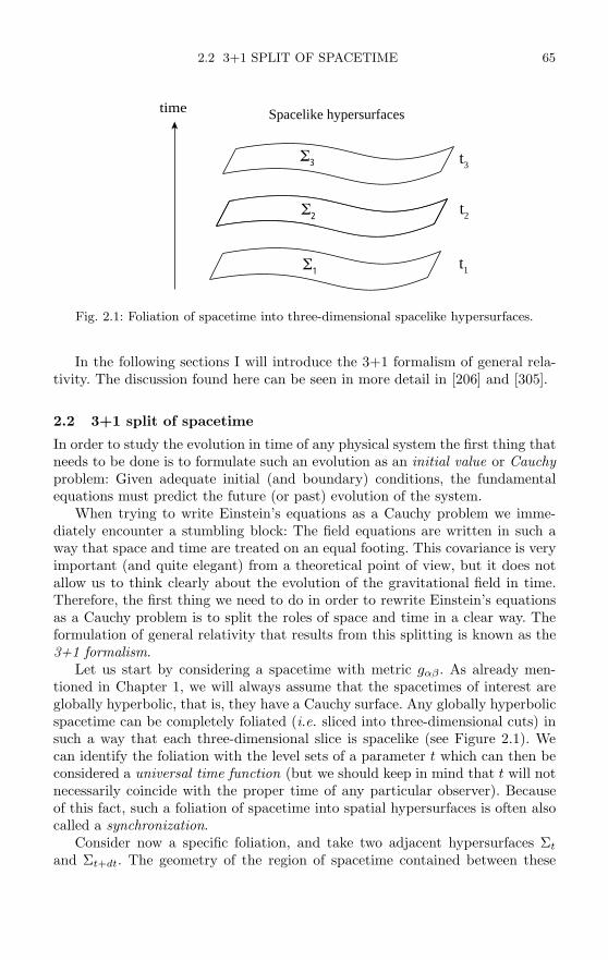
2.2 3+1 SPLIT OF SPACETIME 65
time
3
2
1
t3
t1
t2
Spacelike hypersurfaces
Fig. 2.1: Foliation of spacetime into three-dimensional spacelike hypersurfaces.
In the following sections I will introduce the 3+1 formalism of general rela-tivity. The discussion found here can be seen in more detail in [206] and [305].
2.2 3+1 split of spacetime
In order to study the evolution in time of any physical system the first thing thatneeds to be done is to formulate such an evolution as an initial value or Cauchyproblem: Given adequate initial (and boundary) conditions, the fundamentalequations must predict the future (or past) evolution of the system.
When trying to write Einstein’s equations as a Cauchy problem we imme-diately encounter a stumbling block: The field equations are written in such away that space and time are treated on an equal footing. This covariance is veryimportant (and quite elegant) from a theoretical point of view, but it does notallow us to think clearly about the evolution of the gravitational field in time.Therefore, the first thing we need to do in order to rewrite Einstein’s equationsas a Cauchy problem is to split the roles of space and time in a clear way. Theformulation of general relativity that results from this splitting is known as the3+1 formalism.
Let us start by considering a spacetime with metric gαβ . As already men-tioned in Chapter 1, we will always assume that the spacetimes of interest areglobally hyperbolic, that is, they have a Cauchy surface. Any globally hyperbolicspacetime can be completely foliated (i.e. sliced into three-dimensional cuts) insuch a way that each three-dimensional slice is spacelike (see Figure 2.1). Wecan identify the foliation with the level sets of a parameter t which can then beconsidered a universal time function (but we should keep in mind that t will notnecessarily coincide with the proper time of any particular observer). Becauseof this fact, such a foliation of spacetime into spatial hypersurfaces is often alsocalled a synchronization.
Consider now a specific foliation, and take two adjacent hypersurfaces Σt
and Σt+dt. The geometry of the region of spacetime contained between these

66 THE 3+1 FORMALISM
t
t + dt
dt
xi
xixi – idt
normal line coordinate line
Fig. 2.2: Two adjacent spacelike hypersurfaces. The figure shows the definitions of thelapse function α and the shift vector βi.
two hypersurfaces can be determined from the following three basic ingredients(see Figure 2.2):
• The three-dimensional metric γij (i, j = 1, 2, 3) that measures proper dis-tances within the hypersurface itself:
dl2 = γij dxidxj . (2.2.1)
• The lapse of proper time dτ between both hypersurfaces measured by thoseobservers moving along the direction normal to the hypersurfaces (the so-called normal or Eulerian observers):
dτ = α(t, xi) dt . (2.2.2)
Here α is known as the lapse function.• The relative velocity βi between the Eulerian observers and the lines of
constant spatial coordinates:
xit+dt = xi
t − βi(t, xj) dt , (for Eulerian observers) (2.2.3)
The 3-vector βi is known as the shift vector.
Notice that both the way in which spacetime is foliated, and also the wayin which the spatial coordinate system propagates from one hypersurface to thenext, are not unique. The lapse function α and the shift vector βi are thereforefreely specifiable functions that carry information about our choice of coordinatesystem, and are known as the gauge functions.23
23The notation for lapse and shift used here is common, but certainly not universal. Afrequently used alternative is to denote the lapse function by N , and the shift vector by N i.

2.2 3+1 SPLIT OF SPACETIME 67
In terms of the functions α, βi, γij, the metric of spacetime can be easilyseen to take the following form:
ds2 =(−α2 + βiβ
i)dt2 + 2βi dtdxi + γij dxidxj , (2.2.4)
where we have defined βi := γij βj (from here on we will assume that indices ofpurely spatial tensors are raised and lowered with the spatial metric γij). Thelast equation is known as the 3+1 split of the metric.
More explicitly we have:
gµν =( −α2 + βkβk βi
βj γij
), (2.2.5)
gµν =( −1/α2 βi/α2
βj/α2 γij − βiβj/α2
). (2.2.6)
From the above expressions we can also show that the four-dimensional volumeelement in 3+1 language turns out to be given by
√−g = α√
γ , (2.2.7)
with g and γ the determinants of gµν and γij respectively.Consider now the unit normal vector nµ to the spatial hypersurfaces. It is
not difficult to show that, in the coordinate system just introduced, this vectorhas components given by
nµ =(1/α,−βi/α
), nµ = (−α, 0) . (2.2.8)
Note that this unit normal vector corresponds by definition to the 4-velocity ofthe Eulerian observers.
We can use the normal vector nµ to introduce the 3+1 quantities in a moreformal way that is not tied up with the choice of a coordinate system adaptedto the foliation. The spatial metric γij is simply defined as the metric inducedon each hypersurface Σ by the full spacetime metric gµν :
γµν = gµν + nµnν . (2.2.9)
Notice that written in this way the spatial metric is a full four-dimensional tensor,but when written in the adapted coordinates its time components become trivial.Also, the last expression shows that the spatial metric is nothing more than theprojection operator onto the spatial hypersurfaces.
Consider now our global time function t associated with the foliation. Thelapse function is defined as
α = (−∇t · ∇t)−1/2 . (2.2.10)
(The vector ∇t is clearly timelike because the level sets of t are spacelike). Theunit normal vector to the hypersurfaces can then be expressed in terms of α andt as
nµ = −α∇µt , (2.2.11)where the minus sign is there to guarantee that n is future pointing.

68 THE 3+1 FORMALISM
For the definition of the shift vector we start by introducing three scalarfunctions βi such that when we move from a given hypersurface to the nextfollowing the normal direction, the change in the spatial coordinates is given asbefore by
xit+dt = xi
t − βidt , (2.2.12)
from which we can easily find
βi = −α(n · ∇xi
), (2.2.13)
Thus defined, the βi are scalars, but we can use them to define a 4-vector βby asking for its components in the adapted coordinate system to be given byβµ = (0, βi). The vector constructed in this way is clearly orthogonal to n. Wecan then use the vectors n and β to construct a time vector t defined as
tµ := αnµ + βµ . (2.2.14)
The vector t is nothing more than the tangent vector to the time lines, i.e. thelines of constant spatial coordinates. Notice that, in general, we have tµ = ∇µt.From the above definition we find that t is such that tµnµ = −α, which implies
tµ∇µt = 1 . (2.2.15)
We then find that the shift is nothing more than the projection of t onto thespatial hypersurface
βµ := γµνtν . (2.2.16)
From this we see that we can introduce the shift vector in a completelycoordinate-independent way by first choosing a vector field t satisfying (2.2.15),and then defining the shift through (2.2.16). It is important to stress the factthat the vector field t does not need to be timelike – it can easily be null or evenspacelike (we will later see that this situation frequently arises in the case ofblack hole spacetimes). All we need to ask is that t is not tangent to the spatialhypersurfaces, and that it points to the future, which is precisely the content ofequation (2.2.15). It might seem strange to allow t to be spacelike, since thatwould correspond to a faster than light motion of the coordinate lines, that is, asuperluminal or tachionic shift. But we must remember that it is not a physicaleffect but only the coordinate lines that are moving “faster than light”, and thecoordinates can be chosen freely.
2.3 Extrinsic curvature
When considering the spatial hypersurfaces that constitute the foliation of space-time, we need to distinguish between the intrinsic curvature of those hypersur-faces coming from their internal geometry, and the extrinsic curvature associatedwith the way in which those hypersurfaces are immersed in four-dimensionalspacetime. The intrinsic curvature is given by the three-dimensional Riemann

2.3 EXTRINSIC CURVATURE 69
n
parallel transport
n
Fig. 2.3: The extrinsic curvature tensor is defined as a measure of the change of thenormal vector under parallel transport.
tensor defined in terms of the 3-metric γij . The extrinsic curvature, on the otherhand, is defined in terms of what happens to the normal vector n as it is parallel-transported from one point in the hypersurface to another. In general, we will findthat as we parallel transport this vector to a nearby point, the new vector willnot be normal the hypersurface anymore. The extrinsic curvature tensor Kαβ isa measure of the change of the normal vector under such parallel transport (seeFigure 2.3).
In order to define the extrinsic curvature, we need to introduce the projectionoperator Pα
β onto the spatial hypersurfaces:
Pαβ := δα
β + nαnβ , (2.3.1)
which as we have seen is in fact nothing more than the induced spatial metric,Pαβ = γαβ . Using this projection operator, the extrinsic curvature tensor isdefined as:
Kµν := −Pαµ ∇αnν = − (∇µnν + nµnα∇αnν) , (2.3.2)
As defined above, the tensor Kµν is clearly a purely spatial tensor, that is,nµKµν = nνKµν = 0. This means, in particular, that in a coordinate systemadapted to the foliation we will have K00 = K0i = 0 (though in general we findthat K00 and K0i are not zero). Because of this, we will usually only considerthe spatial components of Kij . Moreover, the tensor Kµν also turns out to besymmetric:
Kµν = Kνµ . (2.3.3)
A couple of remarks are important regarding the definition of Kµν . First,notice that the projection of ∇µnν is crucial in order to make Kµν purely spatial.We could argue that because nµ is unitary, its gradient is necessarily orthogonalto it. This is of course true in the sense that nν∇µ nν = 0, but ∇µnν is in generalnot symmetric and nν∇νnµ = 0 unless the normal lines are geodesic (which is notalways the case). Let us now consider the symmetry of Kµν . As just mentioned∇µnν is not in general symmetric even though nµ is hypersurface orthogonal. Thereason for this is that nα is a unitary vector and thus in general is not equal tothe gradient of the time function t, except when the lapse is unity. However, once

70 THE 3+1 FORMALISM
we project onto the hypersurface, it turns out that Pαµ ∇αnν is indeed symmetric
(the non-symmetry of ∇µnν has to do with the lapse, which is not intrinsic to thehypersurface). In order to see this, consider the congruence of timelike geodesicsorthogonal to Σ, with unit tangent vector ξ. In the neighborhood of Σ consider anew foliation of spacetime given by a time function t such that ξµ = ∇µ t. Since ξis the gradient of a scalar function we clearly will have ∇µξν = ∇νξµ. Moreover,∇µξν will be purely spatial without the need to project it since ξ is tangent tothe timelike geodesics. Now, the vector field n will generally not coincide withξ outside of Σ, but it will coincide within Σ, so its derivatives along directionstangential to Σ must be equal to those of ξ, that is
Pαµ ∇αnν = Pα
µ ∇αξν = ∇µξν = ∇νξµ = Pαν ∇αξµ = Pα
ν ∇αnµ , (2.3.4)
which proves the symmetry of Kµν .Notice, in particular, that the symmetry of the projected part of ∇µnν also
implies that when we contract it with a purely spatial antisymmetric tensor wewill obtain zero, that is
T µν∇µnν = 0 , (2.3.5)
for all Tµν such that Tµν = −Tνµ, nµTµν = 0.From its definition above, it is in fact not difficult to show that the extrinsic
curvature Kµν can be written in an entirely equivalent way as the Lie derivativeof the spatial metric along the normal direction
Kµν = −12
£n γµν . (2.3.6)
That this is so can be easily seen from the definition of the Lie derivative:
£n γµν = nα∇αγµν + γµα∇νnα + γνα∇µnα
= nα∇α (nµnν) + gµα∇νnα + gνα∇µnα
= nαnµ∇αnν + nαnν∇αnµ + ∇νnµ + ∇µnν
=(γα
µ − gαµ
)∇αnν + (γαν − gα
ν )∇αnµ + ∇νnµ + ∇µnν
= γαµ∇αnν + γα
ν ∇αnµ = −2Kµν , (2.3.7)
where we have used the fact that the covariant derivative of gµν is zero and alsothat nα∇µnα = 0. We then find that the extrinsic curvature is essentially the“velocity” of the spatial metric as seen by the Eulerian observers. Notice thatthe extrinsic curvature depends only on the behavior of n within the slice Σ – itis therefore a geometric property of the slice itself.
Now, since n is normal to the hypersurface, it turns out that for any scalarfunction φ we have
£n γµν =1φ
£φn γµν . (2.3.8)
If, in particular, we take as our scalar function the lapse, we find that

2.4 THE EINSTEIN CONSTRAINTS 71
Kµν = − 12α
£αn γµν = − 12α
(£t − £β
)γµν , (2.3.9)
which implies (£t − £β
)γµν = −2αKµν . (2.3.10)
Concentrating now only on the spatial components, and remembering that inthe adapted coordinate system we have £t = ∂t, we finally find
∂tγij − £βγij = −2αKij . (2.3.11)
The last expression can also be rewritten as
∂tγij = −2αKij + Diβj + Djβi , (2.3.12)
where here Di represents the three-dimensional covariant derivative, that is, theone associated with the 3-metric γij , which is in fact nothing more than theprojection of the full four-dimensional covariant derivative: Dµ := Pα
µ ∇α.This brings us half-way to our goal of writing Einstein’s equations as a Cauchy
problem: We already have an evolution equation for the spatial metric γij . Inorder to close the system we still need an evolution equation for Kij . It is im-portant to notice that until now we have only worked with purely geometricconcepts, and we have not used the Einstein field equations at all. It is preciselyfrom the field equations that we will obtain the evolution equations for Kij . Inother words, the evolution equation (2.3.11) for the 3-metric is purely kinematic,while the dynamics of the system will be contained in the evolution equationsfor Kij .
2.4 The Einstein constraints
The true dynamics of the gravitational field are contained in the Einstein fieldequations. In order to proceed further, we need to rewrite these equations in 3+1language. This can be done by considering contractions of these equations withthe normal vector n and with the projector operator onto the hypersurface P µ
ν .We will proceed with this in two stages. In this Section we will consider thosecontractions involving the normal vector, and will leave the rest of the equationsuntil the next Section.
The starting point is to express the four-dimensional Riemann curvaturetensor Rα
βµν in terms of the intrinsic three-dimensional Riemann tensor of thehypersurface itself (3)Rα
βµν , and the extrinsic curvature tensor Kµν . The deriva-tion of these relations is straightforward but rather long, so we will just state thefinal results here (the interested reader can see e.g. [295]). The full projection ofthe Riemann tensor onto the spatial hypersurfaces turns out to be given by theso-called Gauss–Codazzi equations
P δαP κ
β Pλµ P σ
ν Rδκλσ = (3)Rαβµν + KαµKβν − KανKβµ , (2.4.1)

72 THE 3+1 FORMALISM
Similarly, the projection onto the hypersurfaces of the Riemann tensor contractedonce with the normal vector results in the Codazzi–Mainardi equations
P δαP κ
β Pλµ nν Rδκλν = DβKαµ − DαKβµ , (2.4.2)
where as before Dµ = Pαµ ∇α.
In order to start rewriting the Einstein field equations in 3+1 language, noticefirst that
PαµP βνRαβµν = (gαµ + nαnµ)(gβν + nβnν
)Rαβµν
= R + 2nµnνRµν
= 2nµnνGµν , (2.4.3)
with Gµν the Einstein tensor. On the other hand, the Gauss–Codazzi relationsimply that
PαµP βνRαβµν = (3)R + K2 − KµνKµν (2.4.4)
where K := Kµµ is the trace of the extrinsic curvature. We then find
2 nµnνGµν = (3)R + K2 − KµνKµν , (2.4.5)
which through the Einstein equations becomes
(3)R + K2 − KµνKµν = 16πρ , (2.4.6)
where we have defined the quantity ρ := nµnνTµν that corresponds to the localenergy density as measured by the Eulerian observers. Notice that this equationinvolves no explicit time derivatives, so it is not an evolution equation but rathera constraint that must be satisfied at all times. This equation is known as theHamiltonian or energy constraint.
Consider now the mixed contraction of the Einstein tensor. We find,
PαµnνGµν = PαµnνRµν . (2.4.7)
The Codazzi–Mainardi equations then imply
γαµnνGµν = DαK − DµKαµ , (2.4.8)
which again through the field equations becomes
Dµ (Kαµ − γαµK) = 8πjα , (2.4.9)
where now jα := −PαµnνTµν corresponds to the momentum density as measuredby the Eulerian observers. Notice that there are in fact three equations in the lastexpression, as the index α is free, but the case α = 0 is trivial. As before, thereare no time derivatives in these equations so they are also constraints. They areknown as the momentum constraints.

2.5 THE ADM EVOLUTION EQUATIONS 73
In a coordinate system adapted to the foliation, the Hamiltonian and mo-mentum constraints take the final form
(3)R + K2 − KijKij = 16πρ , (2.4.10)
Dj
(Kij − γijK
)= 8πji , (2.4.11)
withρ := nµnνTµν , ji := −P iµnνTµν . (2.4.12)
It is important to notice that the constraints not only do not involve timederivatives, but they are also completely independent of the gauge functions αand βi. This indicates that the constraints are relations that refer purely to agiven hypersurface.
Notice that having a set of constraint equations is not a feature of generalrelativity alone. In electrodynamics we have the Maxwell equations which inthree-dimensional vector calculus notation, and in Gaussian units, take the form
∇ ·E = 4πρ , ∇ · B = 0 , (2.4.13)
∂tE = ∇× B− 4πj , ∂tB = −∇× E , (2.4.14)
where E and B are the electric and magnetic fields respectively, ρ is the chargedensity and j the current density (here ∇ stands for the ordinary flat spacegradient operator and should not be confused with a four-dimensional covariantderivative). The first two equations involving the divergence of the electric andmagnetic fields do not involve time derivatives, so they are in fact constraints,just as in general relativity. The main difference is that Maxwell’s theory hasonly two constraint equations, while general relativity has four (one Hamilto-nian constraint and three momentum constraints). The remaining two Maxwellequations (or rather six since they are vector-valued equations) are the true evo-lution equations for electrodynamics. The corresponding equations for gravitywill be derived in the next Section.
The existence of the constraints implies, in particular, that in the 3+1 formu-lation it is not possible to specify arbitrarily all 12 dynamical quantities γij , Kijas initial conditions. The initial data must already satisfy the constraints, other-wise we will not be solving Einstein’s equations. We will come back to this issuein Chapter 3 when we discuss how to find initial data. The constraints also playother important roles. For example, they are crucial in the Hamiltonian formu-lation of general relativity (see Section 2.7). They are also very important in thestudy of the well-posedness of the system of evolution equations, something wewill have a chance to discuss briefly in Section 2.8 and also in Chapter 5.
2.5 The ADM evolution equations
The Hamiltonian and momentum constraints give us four of the ten independentEinstein field equations, and as we have seen they do not correspond to theevolution equations of the gravitational field, but rather to relations between
74 THE 3+1 FORMALISM
the dynamical variables that must be satisfied at all times. The evolution of thegravitational field is contained in the remaining six field equations.
In order to find these equations we still need the projection onto the hyper-surfaces of the Riemann tensor contracted twice with the normal vector. Thiswill give us the last six independent components of Riemann (the Gauss–Codazziand Gauss–Mainardi equations give us 14 components of Riemann). These pro-jections turn out to be given by
P δµP κ
ν nλnσRδλκσ = £nKµν + KµλKλν +
1α
DµDνα . (2.5.1)
The first thing to notice is that these relations do involve the lapse function α.Also, they make reference to the Lie derivative of the extrinsic curvature alongthe normal direction, which clearly corresponds to evolution in time.
Now, from the Gauss–Codazzi equations (2.4.1) we also find
P δµP κ
ν
(nλnσRδλκσ + Rδκ
)= (3)Rµν + KKµν − KµλKλ
ν , (2.5.2)
which, together with (2.5.1), implies
£tKµν − £βKµν = −DµDνα
+ α(−P δ
µP κν Rδκ + (3)Rµν + KKµν − 2KµλKλ
ν
), (2.5.3)
Using now the Einstein equations written in terms of Rµν , equations (1.13.4),we find
£tKµν − £βKµν = −DµDνα + α[(3)Rµν + KKµν − 2KµλKλ
ν
]+ 4πα [γµν (S − ρ) − 2Sµν ] , (2.5.4)
where ρ is the same as before, and where we have defined Sµν := Pαµ P β
ν Tαβ asthe spatial stress tensor measured by the Eulerian observers (with S := Sµ
µ).Concentrating on the spatial components and again writing £t = ∂t, the lastexpression becomes
∂tKij − £βKij = −DiDjα + α[(3)Rij + KKij − 2KikKk
j
]+ 4πα [γij (S − ρ) − 2Sij ] , (2.5.5)
or expanding the Lie derivative along the shift vector
∂tKij = βk∂kKij + Kki∂jβk + Kkj∂iβ
k − DiDjα
+ α[(3)Rij + KKij − 2KikKk
j
]+ 4πα [γij (S − ρ) − 2Sij ] . (2.5.6)
These equations give us the dynamical evolution of the six independent com-ponents of the extrinsic curvature Kij . Together with equations (2.3.11) for the
2.5 THE ADM EVOLUTION EQUATIONS 75
evolution of the spatial metric they finally allow us to write down the field equa-tions for general relativity as a Cauchy problem. It is important to notice thatwe do not have evolution equations for the gauge quantities α and βi. As wehave mentioned before, these quantities represent our coordinate freedom andcan therefore be chosen freely.
The evolution equations (2.5.5) are known in the numerical relativity com-munity as the Arnowitt–Deser–Misner (ADM) equations. However, as writtenabove, these equations are in fact not in the form originally derived by ADM [31],but they are instead a non-trivial rewriting due to York [305]. It is important tomention exactly what the difference is between the original ADM equations andthe ADM equations a la York, which we will call from now on standard ADM.The two groups of equations differ in two main aspects. In the first place, theoriginal ADM variables are the spatial metric γij and its canonical conjugatemomentum πij coming from the Hamiltonian formulation of general relativity(see the following Section), and which is related to the extrinsic curvature as 24
Kij = − 1√γ
(πij − 1
2γij π
), (2.5.7)
with π = πii and γ the determinant of γij . This change of variables is, of course,
a rather minor detail. However, even if we rewrite the original ADM evolutionequations in terms of Kij , they still differ from (2.5.5) and have the form
∂tKij − £βKij = −DiDjα + α[(3)Rij + KKij − 2KikKk
j
]+ 4πα [γij (S − ρ) − 2Sij ] − αγij
2H , (2.5.8)
with H the Hamiltonian constraint (2.4.10) written as:
H :=12
((3)R + K2 − KijK
ij)− 8πρ = 0 , (2.5.9)
and where the factor 1/2 in the definition of H is there for later convenience.The difference between the ADM and York evolution equations can be traced
back to the fact that the version of ADM comes from the field equations written interms of the Einstein tensor Gµν , whereas the version of York was derived insteadfrom the field equations written in terms of the Ricci tensor Rµν . It is clear thatboth sets of evolution equations for Kij are physically equivalent since they onlydiffer by the addition of a term proportional to the Hamiltonian constraint, whichmust vanish for any physical solution. However, the different evolution equationsfor Kij are not mathematically equivalent. There are basically two reasons whythis is so:
24One must remember that the original goal of ADM was to write a Hamiltonian formulationfor general relativity that could be used as a basis for quantum gravity, and not a system ofevolution equations for dynamical simulations.
76 THE 3+1 FORMALISM
1. In the first place, the space of solutions to the evolution equations is differ-ent in both cases, and only coincides for physical solutions, that is, thosethat satisfy the constraints. In other words, both systems are only equiv-alent in a subset of the full space of solutions. This subset is called theconstraint hypersurface (but notice that this is not a hypersurface in space-time, but instead a hypersurface in the space of solutions to the evolutionequations). Of course, we could always argue that since in the end we areonly interested in physical solutions, this distinction is irrelevant. This isstrictly true only if we can solve the equations exactly. But in the case ofnumerical solutions there will always be some error that will take us out ofthe constraint hypersurface, and the issue then becomes not only relevantbut crucial: If we move slightly off the constraint hypersurface, does thesubsequent evolution remain close to it, or does it diverge rapidly awayfrom it?
2. The second reason why both systems of evolution equations differ math-ematically is related to the last point and is of greater importance. Sincethe Hamiltonian constraint has second derivatives of the spatial metric(hidden inside the Ricci scalar), then by adding a multiple of it to the evo-lution equations we are in fact altering the very structure of the differentialequations.
These types of considerations take us to a fundamental observation that hastoday become one of the most active areas of research associated with numericalrelativity: The 3+1 evolution equations are highly non-unique since we can al-ways add to them arbitrary multiples of the constraints. The different systems ofevolution equations will still coincide in the physical solutions, but might differdramatically in their mathematical properties, and particularly in the way inwhich they react to small violations of the constraints (inevitable numerically).This observation is crucial, and we will come back to it both in Section 2.8, andin Chapter 5.
A final consideration about the 3+1 evolution equations has to do with thepropagation of the constraints: If the constraints are satisfied initially, do theyremain satisfied during the evolution? The answer to this question is, not surpris-ingly, yes, but it is interesting to see how this comes about. In fact it is throughthe Bianchi identities that the propagation of the constraints during the evolu-tion is guaranteed. To see this, we will follow an analysis due to Frittelli [136],and define the following projections of the Einstein field equations
H := nαnβGαβ − 8πρ , (2.5.10)Mµ := −nαP β
µ Gαβ − 8πjµ , (2.5.11)
Eµν := Pαµ P β
ν Gαβ − 8πSµν , (2.5.12)
with ρ, jµ and Sµν defined as before in terms of the stress-energy tensor Tµν . No-tice that here H = 0 corresponds precisely to the Hamiltonian constraint (2.5.9)

2.6 FREE VERSUS CONSTRAINED EVOLUTION 77
(with the correct 1/2 factor), while Mµ = 0 corresponds to the momentum con-straints. On the other hand, Eµν = 0 reduces to the original ADM evolutionequations (multiplied by 2). An important observation is that in this contextYork’s version of the evolution equations in fact corresponds to Eµν − γµνH = 0.The Einstein field equations in terms of these quantities can then be written as
Gµν − 8πTµν = Eµν + nµMν + nνMµ + nµnνH = 0 , (2.5.13)
and the (twice contracted) Bianchi identities imply
∇µ (Eµν + nµMν + nνMµ + nµnνH) = 0 . (2.5.14)
By taking the normal projection and the projection onto the hypersurface of theseidentities and rearranging terms, we obtain the following system of evolutionequations for the constraints
nν∇νH = −DνMν − EµνDµnν + LH(H,Mσ) , (2.5.15)nν∇νMµ = −DνEµν − Eµνnλ∇λnν + LMµ(H,Mσ) , (2.5.16)
where the L’s are shorthand for terms proportional to H and Mµ that haveno derivatives of these quantities. That these are evolution equations for theconstraints can be seen from the fact that the terms on the left hand side arederivatives along the normal direction, i.e. out of the hypersurface. Notice that,if we have initial data such that H = Mµ = 0, and we use the ADM evolutionequations Eµν = 0, the above equations guarantee that on the next hypersurfacethe constraints will still vanish. This proves that the constraints will remainsatisfied. If, on the other hand, we use York’s evolution equations Eµν = γµνH,the same result clearly follows. In fact, it is clear that we could take Eµν to beequal to any combination of constraints.
There is, however, an important difference in the structure of the constraintevolution equations when taking either the ADM or York’s version of the 3+1evolution equations, and we will come back to it later, in Chapter 5. For themoment, it is sufficient to mention that the constraint evolution equations aremathematically well-posed for York’s system, but they are not well posed for theoriginal ADM system, so York’s system should be preferred.
2.6 Free versus constrained evolution
In the previous Sections we have separated the Einstein field equations into evo-lution equations and constraints equations. As already mentioned, the Bianchiidentities guarantee that if the constraints are initially satisfied they will remainsatisfied during the subsequent evolution. This is, however, an exact statement,and since here we are ultimately interested in numerical simulations it is impor-tant to consider the problem of how to evolve the geometric quantities γij andKij while keeping the constraints satisfied. Ideally, we would like to have somediscretized version of the 3+1 evolution equations and constraints that would
78 THE 3+1 FORMALISM
guarantee that the discrete constraints remain satisfied during evolution. Unfor-tunately, such a discretized form of the 3+1 equations is not known to exist atthis time. We must then live with the fact that not all 10 Einstein equations willremain satisfied at the discrete level during a numerical simulation. Of course, weexpect that a good numerical implementation would be such that as we approachthe continuum limit we would recover a solution of the full set of equations.
In practice, we can take two different approaches to the problem of choosingwhich set of equations to solve numerically. The first approach is known as freeevolution, and corresponds to the case when we start with a solution of theconstraint equations as initial data (see Chapter 3), and later advances in timeby solving all 12 evolution equations for γij and Kij . The constraints are thenonly monitored to see how much they are violated during evolution, which givesa rough idea of the accuracy of the simulation. Alternatively, we can choose tosolve some or all of the constraint equations at each time step for a specificsubset of the components of the metric and extrinsic curvature, and evolve theremaining components using the evolution equations. This second approach isknown as constrained evolution.
Constrained evolution is in fact ideal in situations with high degree of sym-metry, like spherical symmetry for example, but is much harder to use in thecase of fully three-dimensional systems. Also, the mathematical properties of aconstrained scheme are much more difficult to analyze in the sense of studyingthe well-posedness of the system of equations (see Chapter 5). And finally, sincethe constraints involve elliptic equations, a constrained scheme is also far slowerto solve numerically in three dimensions than a free evolution scheme. Becauseof all these reasons, in the remainder of the book we will always assume that weare using a free evolution scheme.
For completeness, we should mention a third alternative known as constrainedmetric evolution. In this approach, we choose some extra condition on the metrictensor, such as for example conformal flatness, and impose this condition duringthe whole evolution, thus simplifying considerably the equations to be solved.Such an approach has been used with some success by Wilson and Mathews inhydrodynamical simulations [300]. However, imposing extra conditions on themetric is not in general compatible with the Einstein field equations, and theresults from such simulations should therefore be regarded just as approximationseven in the continuum limit. For example, the condition of conformal flatnessessentially eliminates the gravitational wave degrees of freedom. Whether such anapproximation is good or not will depend on the specific physical system understudy, and the physical information we wish to extract from the simulation.
2.7 Hamiltonian formulation
A field theoretical formulation of general relativity starts from the Hilbert La-grangian which was already introduced in the previous Chapter:
L = R , (2.7.1)

2.7 HAMILTONIAN FORMULATION 79
with R the Ricci scalar of the spacetime. As already mentioned, from a variationalprinciple we can obtain the field equations taking this Lagrangian as the startingpoint.
The Lagrangian formulation of a field theory takes a covariant approach. Inthe first place, the Lagrangian itself must be a scalar function, and also the fieldequations derived from the variational principle come out in fully covariant form.A different approach is to take instead a Hamiltonian formulation of the theory.This approach has important advantages, and in particular is the starting pointof quantum field theory. However, a Hamiltonian formulation requires a cleardistinction to be made between space and time, so it is therefore not covariant.In field theories other than general relativity, and particularly when workingon a flat spacetime background, there is already a natural way in which spaceand time can be split. In general relativity, on the other hand, no such naturalsplitting exists. However, we can take the 3+1 perspective and use this splittingas a basis to construct a Hamiltonian formulation of the theory. Of course, wecan not interpret the time function t directly as a measure of the proper time ofany given observer, since the spacetime metric needed in order to do this is theunknown dynamical variable under study.
The first step in a Hamiltonian formulation is to identify the configurationvariables that describe the state of the field at any given time. For this purposewe will choose the spatial metric variables γij , together with the lapse α andthe co-variant shift vector βi. We now need to rewrite the Hilbert Lagrangian interms of these quantities and their derivatives. Notice that, from the definitionof the Einstein tensor we have
nµnνGµν = nµnνRµν +12
R ⇒ R = 2 (nµnνGµν − nµnνRµν) . (2.7.2)
The first term on the right hand side of the last equation was already obtainedfrom the Gauss–Codazzi relations and is given by equation (2.4.5). For the sec-ond term we use the Ricci identity that relates the commutator of covariantderivatives to the Riemann tensor (equation (1.9.3)):
nµnνRµν = nµnνRλµλν
= nν(∇λ∇νnλ −∇ν∇λnλ
)= ∇λ
(nν∇νnλ
)−∇ν
(nν∇λnλ
)−∇λnν∇νnλ + ∇νnν∇λnλ
= ∇λ
(nν∇νnλ
)−∇ν
(nν∇λnλ
)− KλνKλν + K2 . (2.7.3)
In the previous expression, we have directly identified some terms with the ex-trinsic curvature even though no projection operator is present. We can readilyverify that the contractions in those expressions guarantee that the result follows.The Ricci scalar then takes the form
R = (3)R + KµνKµν − K2 − 2 ∇λ
(nν∇νnλ − nλ∇νnν
). (2.7.4)
The last term in this equation is a total divergence, and since in the end weare only interested in the action S which is an integral of the Lagrangian over a

80 THE 3+1 FORMALISM
given volume Ω, this term can be transformed into an integral over the boundaryof Ω and can therefore be ignored. The Lagrangian of general relativity in 3+1language can then be written as
L = (3)R + KijKij − K2 . (2.7.5)
Notice that L has a similar structure to that of the Hamiltonian constraint, butwith the sign of the quadratic terms in the extrinsic curvature reversed.
To obtain the Lagrangian density L we first need to remember that the four-dimensional volume element in 3+1 adapted coordinates is given by
√−g = α√
γ,so the Lagrangian density takes the form
L = α√
γ((3)R + KijK
ij − K2)
. (2.7.6)
The canonical momenta conjugate to the dynamical field variables are definednow as derivatives of the Lagrangian density with respect to the velocities ofthose fields. For the spatial metric we have the following conjugate momenta
πij :=∂L∂γij
, (2.7.7)
which, using the fact that γij = −2αKij + £βγij , can be reduced to
πij = −√γ(Kij − γijK
). (2.7.8)
By taking now the trace, we can invert this relation between πij and Kij torecover equation (2.5.7):
Kij = − 1√γ
(πij − 1
2γij π
), (2.7.9)
Since the Lagrangian density is independent of any derivatives of the lapse andshift, it is clear that the momenta conjugate to these variables are zero.
The Hamiltonian density is now the defined as
H = πij γij − L , (2.7.10)
which in this case implies
H =[−α
√γ((3)R + K2 − KijK
ij)
+ 2πijDiβj
]. (2.7.11)
After ignoring a total divergence, this can be rewritten as
H = −√γ[α((3)R + K2 − KijK
ij)
+ 2βiDj
(Kij − γijK
)]= −2
√γ[αH + βiMi
], (2.7.12)
2.8 THE BSSNOK FORMULATION 81
with H and Mi defined as before, but without the matter contributions (whichwould arise when we add the Hamiltonian density for the matter). The totalHamiltonian is now defined as
H :=∫
H d3x . (2.7.13)
Variation of this Hamiltonian with respect to α and βi immediately yields theHamiltonian and momentum constraints for vacuum, H = 0 and Mi = 0. Inother words, the lapse and shift behave as Lagrange multipliers for a constrainedsystem.
The evolution equations for the gravitational field now simply follow fromHamilton’s equations:
γij =δHδπij
, πij = − δHδγij
. (2.7.14)
From the first of these equations we find
γij =2α√
γ
(πij − 1
2γijπ
)+ £βγij , (2.7.15)
which is nothing more than the standard evolution equation for γij written interms of πij instead of Kij , and from the second equation we recover the ADMevolution equations for πij , which are equivalent to (2.5.8).
There is an interesting observation we can make at this point, due to An-derson and York [22]. When using the Hamilton equations to derive the 3+1evolution equations, we usually take the lapse function α as an independentquantity to be kept constant during the variation with respect to γij . However,we might take a different point of view and assume that the independent gaugefunction is not the lapse as such, but rather the densitized lapse defined as
α := α/√
γ . (2.7.16)
This change is far from trivial, as keeping α constant alters the dependency ofthe Hamiltonian density on the metric during the variation (we have effectivelymultiplied it by a factor of
√γ). The resulting evolution equations for πij are
now different, and correspond precisely to those of York, equations (2.5.5). Thisobservation points to the fact that perhaps the densitized lapse α is a morefundamental free gauge function than the lapse α itself. We will encounter thedensitized lapse several times throughout the text.
2.8 The BSSNOK formulation
We have already mentioned that the 3+1 evolution equations are in fact non-unique since we can always add to them arbitrary multiples of the constraintsto obtain new evolution equations that are just as valid. In fact, a large number

82 THE 3+1 FORMALISM
of alternative formulations to ADM have been proposed in the literature. InChapter 5, when we discuss the concept of well-posedness of a Cauchy problemand the hyperbolicity of a system of partial differential equations, we will havethe opportunity to discuss some of the different reformulations and why someshould be expected to be better than others in practical applications.
Here, however, we will introduce a specific reformulation that has proven tobe particularly robust in the numerical evolution of a large variety of spacetimes,both with and without matter. Over the past few decades, and particularly sinceresearchers started to work with full three-dimensional evolution codes for nu-merical relativity in the early 1990s, it was realized that the ADM equationslacked the necessary stability properties for long-term numerical simulations,something which is now known to be related to the fact that these equationsare only weakly hyperbolic (see Chapter 5). In 1987, Nakamura, Oohara andKojima presented a reformulation of the ADM evolution equations based on aconformal transformation that showed improved stability properties when com-pared to ADM [215]. This formulation evolved over the following years, though itremained largely unnoticed by the majority of researchers in numerical relativityuntil in 1998 Baumgarte and Shapiro systematically compared it to ADM in aseries of spacetimes showing that the new formulation had far superior stabilityproperties in all cases considered [50]. It was at this point that this reformulationbecame more widely noticed, and today it is used in one form or another by mostlarge three-dimensional codes in numerical relativity. The more common versionof this formulation is based on the work of Shibata and Nakamura [268], andBaumgarte and Shapiro [50], and is commonly known as the BSSN (Baumgarte,Shapiro, Shibata and Nakamura) formulation. This formulation has also beencalled “conformal ADM”, though this name is not particularly good as it failsto make reference to the most important difference between the new formula-tion and ADM. A better name would probably be “conformal Γ formulation”,since as we will see below the crucial element is the introduction of the auxiliaryvariables Γi. However, here we will use the name “BSSNOK formulation” (BS+ Shibata, Nakamura, Oohara and Kojima) in order to make reference to themore commonly used name, and at the same time give due credit to the originalauthors.
In order to introduce the BSSNOK formulation, consider first a conformalrescaling of the spatial metric of the form
γij := ψ−4γij . (2.8.1)
Here ψ is a conformal factor that can in principle be chosen in a number of dif-ferent ways. For example, when evolving black hole spacetimes with conformallyflat initial data, we can simply take ψ to be the initial singular conformal factorand then ask for this conformal factor to remain fixed in time, something thatallows us to evolve only the non-singular part of the metric and is known as thepuncture method for evolutions (see Chapter 6). Alternatively, we can take the

2.8 THE BSSNOK FORMULATION 83
conformal factor to be initially given by some arbitrarily chosen scalar functionand then propose some convenient evolution equation for this scalar function.
In the BSSNOK formulation, we choose the conformal factor in such a waythat the conformal metric γij has unit determinant, that is
ψ4 = γ1/3 ⇒ ψ = γ1/12 , (2.8.2)
with γ the determinant of γij . Furthermore, we ask for this relation to remainsatisfied during the evolution. Now, from (2.3.11) we find that the evolutionequation for the determinant of the metric is
∂tγ = γ(−2αK + 2Diβ
i)
= −2γ(αK − ∂iβ
i)
+ βi∂iγ , (2.8.3)
which implies
∂tψ = −16
ψ(αK − ∂iβ
i)
+ βi∂iψ . (2.8.4)
In practice we usually works with φ = lnψ = 112 ln γ, so that γij = e−4φγij and
∂tφ = −16(αK − ∂iβ
i)
+ βi∂iφ . (2.8.5)
Recently, however, it has been suggested by Campanelli et al. [93] that evolvinginstead χ = 1/ψ4 = exp(−4φ) is a better alternative when considering black holespacetimes for which ψ typically has a 1/r singularity (so that φ has a logarithmicsingularity), while χ is a C4 function at r = 0. For regular spacetimes, of course,it should make no difference if we evolve φ, ψ or χ.
The BSSNOK formulation also separates the extrinsic curvature into its traceK and its tracefree part
Aij = Kij − 13γijK . (2.8.6)
We further make a conformal rescaling of the traceless extrinsic curvature of theform25
Aij = ψ−4Aij = e−4φAij . (2.8.7)
A crucial point is that BSSNOK also introduces three auxiliary variablesknown as the conformal connection functions and defined as
25As we will see in Chapter 3 when we discuss initial data, the “natural” conformal rescal-ing of the traceless extrinsic curvature is in fact Aij = ψ10Aij , which implies Aij = ψ2Aij
(assuming we raise and lower indices of conformal quantities with the conformal metric). SinceI wish to present the standard form of the BSSNOK equations, here I will continue to usethe rescaling Aij = ψ−4Aij . However, in order to avoid possible confusion later, the reader isadvised to keep in mind that this rescaling is different from the one we will use in the nextChapter. It is also important to mention that if we choose to use Aij = ψ2Aij instead, someof the equations in the BSSNOK formulation in fact simplify (most notably the momentumconstraints and the evolution equations for Γi and Aij itself), and it also becomes clear that
the densitized lapse α = αγ−1/2 = αψ−6 plays an important role (the BSSNOK equationswith the natural conformal rescaling can be found in Appendix C).

84 THE 3+1 FORMALISM
Γi := γjkΓijk = −∂j γ
ij , (2.8.8)
where Γijk are the Christoffel symbols of the conformal metric, and where the
second equality comes from the definition of the Christoffel symbols in the casewhen the determinant γ is equal to 1 (which must be true by construction). So,instead of the 12 ADM variables γij and Kij , BSSNOK uses the 17 variablesφ, K, γij , Aij and Γi.26 We can take the point of view that there are only 15dynamical variables since Aij is traceless and γij has unit determinant, but herewe will take the point of view that we are freely evolving all components of Aij
and γij (however, enforcing the constraint A = 0 during a numerical calculationdoes seem to improve the stability of the simulations significantly, so it hasbecome standard practice in most numerical codes).
Up to this point all we have done is redefine variables and introduce threeadditional auxiliary variables. The evolution equation for φ was already foundabove, while those for γij , K and Aij can be obtained directly from the standardADM equations. The system of evolution equations then takes the form27
d
dtγij = −2αAij , (2.8.9)
d
dtφ = −1
6αK , (2.8.10)
d
dtAij = e−4φ
−DiDjα + αRij + 4πα [γij (S − ρ) − 2Sij ]
TF+ α
(KAij − 2AikAk
j
), (2.8.11)
d
dtK = −DiD
iα + α
(AijA
ij +13K2
)+ 4πα (ρ + S) , (2.8.12)
with d/dt := ∂t −£β, and where TF denotes the tracefree part of the expressioninside the brackets. In the previous expressions we have adopted the conventionthat indices of conformal quantities are raised and lowered with the conformalmetric so that, for example, Aij = e4φAij . It is also important to notice that, inthe evolution equation for K, the Hamiltonian constraint has been used in orderto eliminate the Ricci scalar:
R = KijKij − K2 + 16πρ = AijA
ij − 23
K2 + 16πρ . (2.8.13)
We then see how we have already started to add multiples of constraints toevolution equations.
Notice that in the evolution equations for Aij and K there appear covariantderivatives of the lapse function with respect to the physical metric γij . These
26It should be noted that the formulation of [268] uses instead of the Γi the auxiliary variablesFi := −P
j ∂j γij .27From now on, and where there is no possibility of confusion, we will simply drop the index
(3) from the three-dimensional Ricci tensor.
2.8 THE BSSNOK FORMULATION 85
can be easily calculated by using the fact that the Christoffel symbols are relatedthrough:
Γkij = Γk
ij −13(δki Γm
jm + δkj Γm
im − γijγklΓm
lm
)= Γk
ij − 2(δki ∂jφ + δk
j ∂iφ − γijγkl∂lφ
), (2.8.14)
where Γkij are the Christoffel symbols of the conformal metric, and where we
have used the fact that ∂iφ = 112 ∂i ln γ = 1
6 Γmim. This implies, in particular, that
Γi = e4φΓi + 2γij∂jφ . (2.8.15)
In the evolution equation for Aij we also need to calculate the Ricci tensor as-sociated with the physical metric, which can be separated into two contributionsin the following way:
Rij = Rij + Rφij , (2.8.16)
where Rij is the Ricci tensor associated with the conformal metric γij :
Rij = −12γlm∂l∂mγij + γk(i∂j)Γk + ΓkΓ(ij)k
+ γlm(2Γk
l(iΓj)km + ΓkimΓklj
). (2.8.17)
and where Rφij denotes additional terms that depend on φ:
Rφij = −2DiDjφ − 2γijD
kDkφ + 4Diφ Djφ − 4γijDkφ Dkφ , (2.8.18)
with Di the covariant derivative associated with the conformal metric.We must also be careful with the fact that in the evolution equations above
we are computing Lie derivatives with respect to β of tensor densities, that istensors multiplied by powers of the determinant of the metric γ. If a given objectis a tensor times γw/2, then we say that it is a tensor density of weight w. TheLie derivative of a tensor density of weight w is simply given by
£βT =[£βT
]w=0
+ w T ∂iβi , (2.8.19)
where the first term denotes the Lie derivative assuming w = 0, and the secondis the additional contribution due to the density factor. The density weight ofψ = eφ = γ1/12 is clearly 1/6, so the weight of γij and Aij is −2/3, and theweight of γij is 2/3. In particular we have
£βφ = βk∂kφ +16
∂kβk , (2.8.20)
£β γij = βk∂kγij + γik∂jβk + γjk∂iβ
k − 23γij∂kβk . (2.8.21)
There are several motivations for the change of variables introduced above.First, the conformal transformation and the separating out of the trace of the

86 THE 3+1 FORMALISM
extrinsic curvature are done in order to have better control over the slicing con-ditions that, as we will see in Chapter 4, are generally related with the trace ofKij . On the other hand, the introduction of the conformal connection variablesΓi has the important consequence that when these functions are considered asindependent variables, then the second derivatives of the conformal metric thatappear on the right hand side of equation (2.8.11) (contained in the Ricci ten-sor (2.8.17)) reduce to the simple scalar Laplace operator γlm∂l∂mγij . All otherterms with second derivatives of γij have been rewritten in terms of first deriva-tives of the Γi.
If the Γi are to be considered as independent variables, we are of course stillmissing an evolution equation for them. This equation can be obtained directlyfrom (2.8.8) and (2.3.11):
∂tΓi = −∂j
(£βγij
)− 2
(α∂jA
ij + Aij∂jα)
, (2.8.22)
which after expanding out the Lie derivative term becomes
∂tΓi = γjk∂j∂kβi +13
γij∂j∂kβk + βj∂jΓi − Γj∂jβi +
23
Γi∂jβj
− 2(α∂jA
ij + Aij∂jα)
.
The last three terms of the first line clearly form the Lie derivative for a vectordensity of weight 2/3, while the extra terms involving second derivatives of theshift arise from the fact that the Γi are not really components of a vector den-sity, but are rather contracted Christoffel symbols. Bearing this in mind we canrewrite the last equation in more compact form as
d
dtΓi = γjk∂j∂kβi +
13
γij∂j∂kβk − 2(α∂jA
ij + Aij∂jα)
. (2.8.23)
We are still missing one key element of the BSSNOK formulation. In practiceit turns out to be that, in spite of the motivations mentioned above, if we useequations (2.8.9), (2.8.10), (2.8.11), (2.8.12), and (2.8.23) in a numerical simula-tion the system turns out be violently unstable. In order to fix this problem weneed to consider the momentum constraints, which in terms of the new variablestake the form
∂jAij = −Γi
jkAjk − 6Aij∂jφ +23γij∂jK + 8πji , (2.8.24)
with ji := e4φji. We can now use this equation to substitute the divergence ofAij that appears in the evolution equation for the Γi. We find:
d
dtΓi = γjk∂j∂kβi +
13
γij∂j∂kβk − 2Aij∂jα
+ 2α
(Γi
jkAjk + 6Aij∂jφ − 23γij∂jK − 8πji
). (2.8.25)

2.9 ALTERNATIVE FORMALISMS 87
The final system of evolution equations is then (2.8.9), (2.8.10), (2.8.11),(2.8.12), and (2.8.25). This new system not only does not present the violentinstability mentioned before, but it also turns out to be far more stable thanADM in all cases studied until now. That this is so was first shown empirically(that is, through direct comparison of numerical simulations) by Baumgarte andShapiro [50], and was later put on somewhat firmer ground by Alcubierre et al. [6]by considering linear perturbations of flat space. However, a full understanding ofwhy BSSNOK is much more robust that ADM will have to wait until Chapter 5when we discuss the concept of hyperbolicity.
The use of the momentum constraints to modify the evolution equation forthe Γi is the key ingredient of the BSSNOK formulation, and it is used in one wayor another in all current implementations of this system of equations. There aresome additional tricks that have been developed by different groups to make thenumerical simulations even better behaved, like actively forcing the trace of theconformal-traceless extrinsic curvature Aij to remain zero during the evolutionand using the independently evolved Γi only in terms where derivatives of thesefunctions appear, but we will not go into such details here.
2.9 Alternative formalisms
In this Chapter we have discussed the 3+1, or Cauchy, formalism for studying theevolution of spacetime. However, it is also important to mention other approachesto the problem of constructing a solution of Einstein’s equations given adequateinitial data. I will consider here two alternative approaches that have importantstrengths, namely the characteristic formulation and the conformal approach.The discussion here will be very brief, focusing mainly on the basic ideas behindeach approach.
2.9.1 The characteristic approach
The characteristic formulation originates from the idea of using a foliation ofspacetime based not on spacelike but rather on null hypersurfaces. Here we willdiscuss the main ideas behind this approach only briefly; a more detailed discus-sion can be found in the review paper by Winicour [301].
The idea of using null hypersurfaces is very attractive if we are interested inextracting gravitational wave information from an astrophysical system. Whenworking with spatial hypersurfaces, this extraction typically requires the use ofperturbative expansions around some Schwarzschild background (see Chapter 8)that in theory only work well at infinity. On the other hand, there is a completelyunambiguous and rigorous description of gravitational waves on null hypersur-faces even in the non-linear context. This is the main motivation for the use of thecharacteristic approach, but it has yet another important advantage. In practice,in numerical simulations we can only evolve a finite region of spacetime, so whenusing spatial hypersurfaces we are forced to introduce some artificial boundarycondition at a finite distance. Rigorous outgoing wave boundary conditions can

88 THE 3+1 FORMALISM
(a) (b) (c)
Fig. 2.4: Domain of dependence for the characteristic formulation. (a) A single nullhypersurface has an empty domain of dependence as there are light rays coming frominfinity that pass arbitrarily close to it but never intersect it. (b) The double nullapproach uses two null hypersurfaces. (c) A different approach is to use a centraltimelike world-tube (or world-line) to have a non-trivial domain of dependence.
in fact only be imposed at asymptotic null infinity, so the use of hypersurfacesthat are null far away is ideal for this purpose.
There are, however, two important points to consider when using null hyper-surfaces. The first is that even relatively small perturbations can cause the lightrays generating such a hypersurface to cross, leading to the formation of causticswhich are very difficult to handle numerically. The other point to consider is thatthe domain of dependence of a single regular null hypersurface is always empty.This is easy to understand as there can always be light rays coming from infinitythat will come arbitrarily close to any point in the hypersurface without evertouching it, no matter how far the hypersurface extends. It turns out then thatwe must always add a second boundary surface in order to have a non-trivialfuture domain of dependence. Typical choices are to use either a second nullhypersurface (the double null approach), or a central timelike world-tube thatin some cases is collapsed to a single world-line (see Figure 2.4).
In the characteristic approach, we consider a foliation of null hypersurfacescorresponding to the level sets of a coordinate function u. On each hypersur-face, different generating light rays are identified with angular coordinates xA
(A = 2, 3), and an extra radial coordinate λ is used to parameterize these rays.In terms of these coordinates, the Einstein field equations take the followingschematic form:
∂λF = HF (F, G) , (2.9.1)∂u∂λG = HG (F, G, ∂uG) , (2.9.2)
where F is a set of geometric variables related to the null hypersurface and Ga set of evolution variables. The functions HF and HG are non-linear operatorsacting on the values of the variables on the hypersurface. The specific form ofthe equations depends on the choice of the form of the metric and other details.
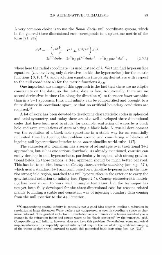
2.9 ALTERNATIVE FORMALISMS 89
A very common choice is to use the Bondi–Sachs null coordinate system, whichin the general three-dimensional case corresponds to a spacetime metric of theform [71, 247]
ds2 = −(
e2βV
r− r2hABUAUB
)du2
− 2e2βdudr − 2r2hABUBdudxA + r2hABdxAdxB , (2.9.3)
where here the radial coordinate r is used instead of λ. We then find hypersurfaceequations (i.e. involving only derivatives inside the hypersurface) for the metricfunctions β, V, UA, and evolution equations (involving derivatives with respectto the null coordinate u) for the metric functions hAB.
One important advantage of this approach is the fact that there are no ellipticconstraints on the data, so the initial data is free. Additionally, there are nosecond derivatives in time (i.e. along the direction u), so there are fewer variablesthan in a 3+1 approach. Plus, null infinity can be compactified and brought to afinite distance in coordinate space, so that no artificial boundary conditions arerequired.28
A lot of work has been devoted to developing characteristic codes in sphericaland axial symmetry, and today there are also well-developed three-dimensionalcodes that have been used to study, for example, scattering of waves by a blackhole and even simulations of stars orbiting a black hole. A crucial developmentwas the evolution of a black hole spacetime in a stable way for an essentiallyunlimited time by turning the problem around and considering a foliation ofingoing null hypersurfaces interior to an outer timelike world-tube [147].
The characteristic formalism has a series of advantages over traditional 3+1approaches, but is has one serious drawback. As already mentioned, caustics caneasily develop in null hypersurfaces, particularly in regions with strong gravita-tional fields. In those regions, a 3+1 approach should be much better behaved.This has led to an idea known as Cauchy-characteristic matching (see e.g. [57]),which uses a standard 3+1 approach based on a timelike hypersurface in the inte-rior strong field region, matched to a null hypersurface in the exterior to carry thegravitational radiation to infinity (see Figure 2.5). Cauchy-characteristic match-ing has been shown to work well in simple test cases, but the technique hasnot yet been fully developed for the three-dimensional case for reasons relatedmainly to finding a stable and consistent way of injecting boundary data comingfrom the null exterior to the 3+1 interior.
28Compactifying spatial infinity is generally not a good idea since it implies a reduction inresolution at large distances: Wave packets get compressed as seen in coordinate space as theymove outward. This gradual reduction in resolution acts on numerical schemes essentially as achange in the refraction index and causes waves to be “back-scattered” by the numerical grid.Compactifying null infinity, however, does not have this problem. Nevertheless, some numericalimplementations do compactify spatial infinity but require the use of strong artificial dampingof the waves as they travel outward to avoid this numerical back-scattering (see e.g. [231]).
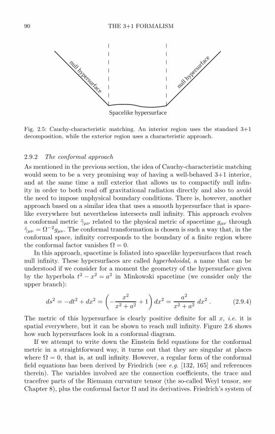
90 THE 3+1 FORMALISM
Spacelike hypersurface
null
hype
rsurfa
cenull hypersurface
Fig. 2.5: Cauchy-characteristic matching. An interior region uses the standard 3+1decomposition, while the exterior region uses a characteristic approach.
2.9.2 The conformal approachAs mentioned in the previous section, the idea of Cauchy-characteristic matchingwould seem to be a very promising way of having a well-behaved 3+1 interior,and at the same time a null exterior that allows us to compactify null infin-ity in order to both read off gravitational radiation directly and also to avoidthe need to impose unphysical boundary conditions. There is, however, anotherapproach based on a similar idea that uses a smooth hypersurface that is space-like everywhere but nevertheless intersects null infinity. This approach evolvesa conformal metric γµν related to the physical metric of spacetime gµν throughγµν = Ω−2gµν . The conformal transformation is chosen is such a way that, in theconformal space, infinity corresponds to the boundary of a finite region wherethe conformal factor vanishes Ω = 0.
In this approach, spacetime is foliated into spacelike hypersurfaces that reachnull infinity. These hypersurfaces are called hyperboloidal, a name that can beunderstood if we consider for a moment the geometry of the hypersurface givenby the hyperbola t2 − x2 = a2 in Minkowski spacetime (we consider only theupper branch):
ds2 = −dt2 + dx2 =(− x2
x2 + a2+ 1)
dx2 =a2
x2 + a2dx2 . (2.9.4)
The metric of this hypersurface is clearly positive definite for all x, i.e. it isspatial everywhere, but it can be shown to reach null infinity. Figure 2.6 showshow such hypersurfaces look in a conformal diagram.
If we attempt to write down the Einstein field equations for the conformalmetric in a straightforward way, it turns out that they are singular at placeswhere Ω = 0, that is, at null infinity. However, a regular form of the conformalfield equations has been derived by Friedrich (see e.g. [132, 165] and referencestherein). The variables involved are the connection coefficients, the trace andtracefree parts of the Riemann curvature tensor (the so-called Weyl tensor, seeChapter 8), plus the conformal factor Ω and its derivatives. Friedrich’s system of
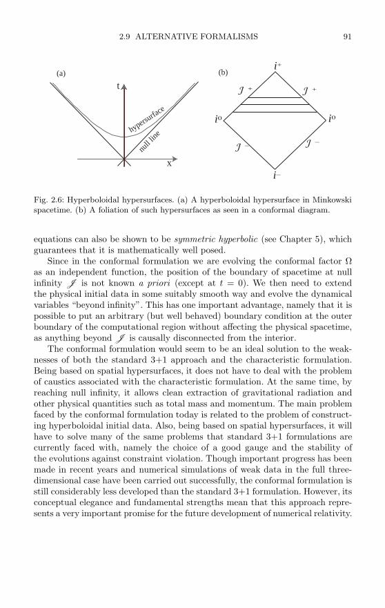
2.9 ALTERNATIVE FORMALISMS 91
t
x
hypersurfa
ce
null
line
i0i0
i+
i–
J +J +
J –J –
(a) (b)
Fig. 2.6: Hyperboloidal hypersurfaces. (a) A hyperboloidal hypersurface in Minkowskispacetime. (b) A foliation of such hypersurfaces as seen in a conformal diagram.
equations can also be shown to be symmetric hyperbolic (see Chapter 5), whichguarantees that it is mathematically well posed.
Since in the conformal formulation we are evolving the conformal factor Ωas an independent function, the position of the boundary of spacetime at nullinfinity J is not known a priori (except at t = 0). We then need to extendthe physical initial data in some suitably smooth way and evolve the dynamicalvariables “beyond infinity”. This has one important advantage, namely that it ispossible to put an arbitrary (but well behaved) boundary condition at the outerboundary of the computational region without affecting the physical spacetime,as anything beyond J is causally disconnected from the interior.
The conformal formulation would seem to be an ideal solution to the weak-nesses of both the standard 3+1 approach and the characteristic formulation.Being based on spatial hypersurfaces, it does not have to deal with the problemof caustics associated with the characteristic formulation. At the same time, byreaching null infinity, it allows clean extraction of gravitational radiation andother physical quantities such as total mass and momentum. The main problemfaced by the conformal formulation today is related to the problem of construct-ing hyperboloidal initial data. Also, being based on spatial hypersurfaces, it willhave to solve many of the same problems that standard 3+1 formulations arecurrently faced with, namely the choice of a good gauge and the stability ofthe evolutions against constraint violation. Though important progress has beenmade in recent years and numerical simulations of weak data in the full three-dimensional case have been carried out successfully, the conformal formulation isstill considerably less developed than the standard 3+1 formulation. However, itsconceptual elegance and fundamental strengths mean that this approach repre-sents a very important promise for the future development of numerical relativity.

3
INITIAL DATA
3.1 IntroductionAs we saw in the previous Chapter, out of the ten Einstein field equations only sixcontain time derivatives and therefore represent the true evolution equations ofthe spacetime geometry. The remaining four equations are constraints that mustbe satisfied at all times. These are the Hamiltonian and momentum constraints,which for concreteness we will rewrite here in a 3+1 adapted coordinate system
(3)R + K2 − KijKij = 16πρ , (3.1.1)
Dj
(Kij − γijK
)= 8πji , (3.1.2)
with ρ and ji the energy and momentum densities seen by the Eulerian (normal)observers and defined as
ρ := nµnνTµν , ji := −P iµnνTµν . (3.1.3)
The existence of the constraint equations implies that it is not possible ingeneral to choose arbitrarily all 12 dynamical quantities γij , Kij as initial data.The initial data has to be chosen in such a way that the constraints are satisfiedfrom the beginning, otherwise we will not be solving Einstein’s equations. Thismeans that before starting an evolution, it is necessary to first solve the initialdata problem to obtain adequate values of γij , Kij that represent the physicalsituation that we are interested in.
The constraints form a system of four coupled partial differential equationsof elliptic type, and in general they are difficult to solve. Still, there are severalwell-known procedures to solve these equations in specific circumstances. Untila few years ago, the most common procedure was the conformal decompositionof York and Lichnerowicz [189, 303, 304]. More recently, the so-called conformalthin-sandwich approach [307] has become more and more popular when solvingthe constraints, as it allows for a clearer interpretation of the freely specifiabledata. In this Chapter we will consider both these approaches to the problem offinding initial data. As a particular application of these techniques, we will alsoconsider the special case of initial data for black hole spacetimes. A recent reviewby Cook of the initial data problem in numerical relativity can be found in [102].
3.2 York–Lichnerowicz conformal decompositionWhen trying to solve the constraint equations one is immediately faced withthe problem of having four differential equations for the 12 degrees of freedom
92

3.2 YORK–LICHNEROWICZ CONFORMAL DECOMPOSITION 93
associated with the spatial metric and extrinsic curvature γij , Kij. The firstquestion that must be answered is which of those 12 quantities will be taken asfree data, and which will be solved for using the constraints. Except in very simplecases like that of the linearized theory, there is no natural way of identifying whichare the “true” dynamical components and which are the constrained components.One must therefore develop some procedure that chooses eight components asfree data and allows one to solve for the remaining four in a clear way. The mostcommon procedure for doing this is known as the York–Lichnerowicz conformaldecomposition.
The York–Lichnerowicz conformal decomposition starts from a conformaltransformation of the 3-metric of the form29
γij = ψ4γij , (3.2.1)
where the conformal metric γij is considered as given. It is not difficult to showthat, in terms of the conformal metric, the Hamiltonian constraint takes the form
8D2ψ − R ψ + ψ5(KijK
ij − K2)
+ 16πψ5ρ = 0 , (3.2.2)
where D2 and R are the Laplace operator and Ricci scalar associated with γij .The extrinsic curvature is also separated into its trace K and its tracefree
part given by
Aij = Kij − 13γij K . (3.2.3)
The Hamiltonian constraint then becomes
8D2ψ − R ψ + ψ5(
AijAij − 2
3K2
)+ 16πψ5ρ = 0 . (3.2.4)
Notice that we have transformed the Hamiltonian constraint into an elliptic equa-tion for the conformal factor ψ, and solving it will clearly allow us to reconstructthe full physical metric γij from a given conformal metric γij .
Let us now consider the momentum constraints, which in terms of Aij takethe form
DjAij − 2
3DiK − 8πji = 0 . (3.2.5)
In order to transform the momentum constraints into three equations forthree unknowns, we can now use a general algebraic result that states that anysymmetric-tracefree tensor Sij can be split in the following way
Sij = Sij∗ + (LW )ij
, (3.2.6)
29In order to avoid confusion we will denote conformal quantities here with an over-barinstead of a tilde. The tilde will be used only for the specific conformal transformation thatfactors out the volume element for which ψ = γ1/12 (as in the BSSNOK formulation discussedin Chapter 2).
94 INITIAL DATA
where Sij∗ is a symmetric, traceless and transverse tensor (i.e. with zero diver-
gence DjSij∗ = 0), W i is a vector, and L is an operator defined as
(LW )ij := DiW j + DjW i − 23
γijDkW k , (3.2.7)
The quantity (LW )ij is known as the conformal Killing form associated withthe vector W i, and its contribution is called the longitudinal part of Sij . If theconformal Killing form vanishes, then the vector W i is called a conformal Killingvector, since in that case one has
£ W
(γ−1/3γij
)= DiWj + DjWi − 2
3γijDkW k = (LW )ij = 0 , (3.2.8)
that is, the conformal metric γij = γ−1/3γij with the volume element factoredout is invariant along the vector field (one should not confuse γij , which has unitvolume element, with γij which has a volume element given by γ = γ/ψ12).
Notice that the operator L can be defined using any metric tensor. Twonatural choices present themselves at this point for the decomposition of Aij :One can use the operator L associated with the conformal metric, or the oper-ator L associated with the physical metric. We will consider both these casesin turn, and later introduce a different type of tensor splitting that resolves theincompatibility between the first two approaches.
3.2.1 Conformal transverse decomposition
We start by performing a conformal transformation on Aij in the following way
Aij = ψ10Aij . (3.2.9)
The factor of ψ10 is chosen since one can easily show that for any symmetric-tracefree tensor Sij the following identity holds
DjSij = ψ−nDj
(ψnSij
)+ (10 − n)Sik∂k lnψ , (3.2.10)
where as before Di is the covariant derivative associated with the conformalmetric. The choice n = 10 is therefore clearly natural.30 Notice that we willraise and lower indices of conformal tensors with the conformal metric, so thatin particular we find Aij = ψ2Aij . In terms of Aij the momentum constraintsbecome
DjAij − 2
3ψ6DiK − 8πψ10ji = 0 , (3.2.11)
We now apply the transverse decomposition to Aij using the operator Lassociated with the conformal metric γij :
30To avoid confusion, the reader is reminded that when discussing the BSSNOK formulationin the last Chapter the alternative, less “natural”, rescaling Aij = ψ4Aij was used in order torecover the standard form of this formulation.

3.2 YORK–LICHNEROWICZ CONFORMAL DECOMPOSITION 95
Aij = Aij∗ +
(LW
)ij. (3.2.12)
From this one can easily show that the momentum constraints reduce to
∆L W i − 23ψ6DiK − 8πψ10ji = 0 , (3.2.13)
where we have defined
∆L W i := Dj(LW )ij
= D2W i + DjDiW j − 2
3DiDjW
j
= D2W i +13
DiDjWj + Ri
jWj . (3.2.14)
The conformal Ricci tensor Rij appears in the last expression when we commute
covariant derivatives. Equations (3.2.13) clearly form a set of three coupled el-liptic equations for W i.
Let us now assume that we are given the conformal metric γij , the traceof the extrinsic curvature K, and the transverse-traceless part of the conformalextrinsic curvature Aij
∗ . We can then use the Hamiltonian constraint (3.2.4) andmomentum constraints (3.2.13) to find the conformal factor ψ and the vectorW i, and thus reconstruct the physical metric γij and extrinsic curvature Kij .
There is still, however, an important point to consider here. Even though itis a simple task to find a symmetric-tracefree tensor, it is quite a different matterto construct a transverse tensor. In order to construct such a tensor one needsto start from an arbitrary symmetric-tracefree tensor M ij that is not necessarilytransverse. Its transverse part can clearly be expressed as
M ij∗ = M ij − (LY
)ij, (3.2.15)
for some vector Y i still to be determined. Now, since M ij∗ is transverse by defi-
nition, the following relation between Y i and M ij must hold
∆L Y i = DjMij . (3.2.16)
Given M ij , this equation must be solved to find the vector Y i, which will in turnallows us to construct the transverse tensor M ij
∗ .The above procedure can in fact be incorporated into the solution of the
constraints. Taking Aij∗ = M ij
∗ we will have
Aij = M ij∗ +
(LW
)ij = M ij +(LV)ij
, (3.2.17)
with V i := W i− Y i, and where we have used the fact that L is a linear operator.

96 INITIAL DATA
One can now rewrite the Hamiltonian and momentum constraints in termsof Aij , V i and M ij to find
8D2ψ − R ψ + ψ−7AijAij − 2
3ψ5K2 + 16πψ5ρ = 0 , (3.2.18)
∆L V i + DjMij − 2
3ψ6DiK − 8πψ10ji = 0 . (3.2.19)
It is common to define ρ := ψ8ρ and ji := ψ10ji as the conformally rescaledenergy and momentum densities. The weight of the conformal factor in the def-inition of ji is chosen in order to eliminate factors of ψ from the matter termsin the momentum constraints and thus decouple them more easily from theHamiltonian constraint. The weight of ψ in the definition of ρ is then fixed forconsistency reasons (for example, ρ2 and jkjk must have the same power of ψwhen written in terms of conformal quantities for the energy conditions to beindependent of ψ).
Equations (3.2.18) and (3.2.19) are to be solved for ψ and V i, with free datagiven in the form of the conformal metric γij , a symmetric-tracefree tensor M ij ,the trace of the extrinsic curvature K, and the energy and momentum densitiesρ and ji. The physical quantities are then reconstructed as
γij = ψ4γij , (3.2.20)
Kij = ψ−10Aij +13
γijK , (3.2.21)
withAij =
(LV)ij + M ij . (3.2.22)
The equations just found are the most common way of writing the constraintsin the York–Lichnerowicz approach.31
Notice how all four equations are coupled with each other. A way to sim-plify the problem considerably is to simply choose K constant, corresponding toa constant mean curvature spatial hypersurface, in which case the momentumconstraints decouple completely from the Hamiltonian constraint. One wouldthen start by solving the momentum constraints (3.2.19) for V i, use this toreconstruct Aij , and only later solve the Hamiltonian constraint (3.2.18) for ψ.
The problem simplifies even more if, apart from taking K constant, one alsotakes the conformal metric to be the one corresponding to flat space (i.e. thephysical metric is conformally flat). The Hamiltonian constraint then reduces to
8D2flatψ + ψ−7AijA
ij − 23ψ5K2 + 16πψ5ρ = 0 , (3.2.23)
where now D2flat is just the flat space Laplacian. In the particular case of time-
symmetric initial data, corresponding to Kij = 0 at t = 0, the momentum
31In fact, Lichnerowicz found the expression for the conformal decomposition of the Hamil-tonian constraint [189], but the full decomposition of the momentum constraints is due toYork [303, 304].
3.2 YORK–LICHNEROWICZ CONFORMAL DECOMPOSITION 97
constraints are trivially satisfied. If, moreover, we assume that we are in vacuumthe Hamiltonian constraint reduces even further to
D2flatψ = 0 , (3.2.24)
which is nothing more than the standard Laplace equation. We will come backto this equation later when we study black hole initial data.
3.2.2 Physical transverse decomposition
Let us now consider the transverse decomposition of Aij (without a conformalrescaling), using the operator L associated with the physical metric γij :
Aij = Aij∗ + (LW )ij
. (3.2.25)
The momentum constraints then take the form
∆L W i − 23DiK − 8πji = 0 . (3.2.26)
We now need to rewrite the covariant derivative operators in this expression interms of the conformal metric. Notice first that if we take
Wi = ψnWi ⇒ W i = ψ(n−4)W i , (3.2.27)
then in general one finds that
(LW )ij = ψn(LW
)ij
+ ψn (n − 4)[Wi∂j ln ψ + Wj∂i ln ψ − 2
3γijW
k∂k lnψ
]. (3.2.28)
Taking n = 4 therefore results in
(LW )ij = ψ4(LW
)ij
⇒ (LW )ij = ψ−4 (LW)ij
, (3.2.29)
with W i = W i (so that the contra-variant vector W i remains equal to itselfunder a conformal rescaling). Using now the relation (3.2.10) with n = 4 we find
∆L W i = Dj (LW )ij = Dj
[ψ−4 (LW
)ij]= ψ−4
[Dj
(LW
)ij+ 6
(LW
)ij∂j lnψ
]= ψ−4
[∆L W i + 6
(LW
)ij∂j lnψ
]. (3.2.30)
The momentum constraints then become
∆L W i + 6(LW
)ij∂j ln ψ − 2
3DiK − 8πψ4ji = 0 , (3.2.31)
where we used ψ4DiK = ψ4γij∂jK = γij∂jK = DiK.
98 INITIAL DATA
Just as before, we will incorporate the procedure for obtaining the transversepart of a general symmetric-tracefree tensor into the solution of the constraints.What we want is to obtain the transverse part of Aij , that is Aij
∗ , which hasnot been conformally rescaled. Assuming then that we are given a symmetric-tracefree tensor M ij , its transverse part can clearly be written as
M ij∗ = M ij − (LY )ij
, (3.2.32)
for some vector Y i. As before, the fact that M ij∗ implies that the following
relation must hold:∆L Y i = DjM
ij , (3.2.33)
but notice that all quantities here are in the physical space. Taking now Aij∗ =
M ij∗ , we then have
Aij = M ij + (LV )ij , (3.2.34)
with V i := W i − Y i.Combining all previous results, the momentum constraints become,
∆L V i + 6(LV)ij
∂j ln ψ + ψ4DjMij − 2
3DiK − 8πψ4ji = 0 , (3.2.35)
where as before we have used V i = V i.The last expression, however, still has the divergence DjM
ij written in termsof the physical metric. In order to express the momentum constraints completelyin terms of the conformal metric we take M ij = ψ10M ij . Using again (3.2.10),we can rewrite the momentum constraints in the final form
∆L V i + 6(LV)ij
∂j ln ψ + ψ−6DjMij − 2
3DiK − 8πψ4ji = 0 . (3.2.36)
The full system of equations to be solved is then
8D2ψ − R ψ + ψ5(
AijAij − 2
3K2
)+ 16πψ5ρ = 0 , (3.2.37)
∆L V i + 6(LV)ij
∂j ln ψ + ψ−6DjMij − 2
3DiK − 8πψ4ji = 0 , (3.2.38)
with the physical quantities reconstructed as
γij = ψ4γij , (3.2.39)
Kij = Aij +13
γijK , (3.2.40)
withAij = ψ−4 (LV
)ij + ψ−10M ij . (3.2.41)
Notice that we have the same set of initial data as before, namely γij , M ij , Kand the energy and momentum densities ρ and ji. The Hamiltonian constraint
3.2 YORK–LICHNEROWICZ CONFORMAL DECOMPOSITION 99
is in fact identical to equation (3.2.18) when we remember that Aij = ψ10Aij ,but the momentum constraint differs from (3.2.19) in both the powers of ψ inseveral terms and the fact that there is an extra term involving derivatives of ψ.
The difference between the two versions of the momentum constraints,(3.2.19) and (3.2.38), can be seen more easily if we notice that
ψ−nDj
[ψn(LV)ij] = ∆L V i + n
(LV)ij
∂j lnψ , (3.2.42)
so that (3.2.38) can in fact be rewritten as
Dj
[ψ6(LV)ij]+ DjM
ij − 23ψ6DiK − 8πψ10ji = 0 . (3.2.43)
Comparing with (3.2.19) we see that the two equations are identical except forthe factor ψ6 inside the divergence in the first term. So there is a weight differencein the conformal rescaling and as a consequence the momentum constraints arenow more tightly coupled with the Hamiltonian constraint. In particular, themomentum constraints now do not decouple from the Hamiltonian constraintfor K constant.
It is clear that starting from identical free data we will then obtain differentphysical data if we use the conformal or physical transverse decompositions.Of course, we will obtain consistent solutions of the constraints in both casesthat will represent roughly the same physical situation, but there will be cleardifferences.
3.2.3 Weighted transverse decomposition
In the previous Section we considered the conformal and physical transversedecomposition of the extrinsic curvature and arrived at different forms of themomentum constraint. The conformal transverse decomposition results in some-what simpler equations, and because of this it has been used more in practice.Still, the existence of two different methods of splitting the traceless extrinsiccurvature suggests that perhaps neither is optimal. The root of the problem liesin the fact that the conformal rescaling and tensor splitting do not commute.
More explicitly, from equation (3.2.10) we learn that the natural conformaltransformation for a symmetric-tracefree tensor is
Aij = ψ−10Aij . (3.2.44)
However, equation (3.2.28) shows that the natural conformal transformation ofthe longitudinal part is instead
(LW )ij = ψ−4 (LW)
. (3.2.45)
The mismatched powers of ψ in these transformation rules are at the root of thenon-commutativity of conformal transformation and tensor splitting.
100 INITIAL DATA
Recently, however, Pfeiffer and York have introduced a new splitting of ten-sors that completely resolves the problem [226]. The main idea is to split thetraceless extrinsic curvature Aij as
Aij = Aij∗ +
1σ
(LW )ij, (3.2.46)
with σ a positive definite scalar. One then introduces the following conformaltransformations
Aij∗ = ψ10Aij , W i = W i , σ = ψ−6σ . (3.2.47)
The new splitting then has the important property that
Aij = Aij∗ +
1σ
(LW )ij
= ψ−10[Aij
∗ +1σ
(LW
)ij] = ψ−10Aij , (3.2.48)
so conformal transformation and tensor splittings are now fully consistent.32
With this splitting the momentum constraints become
Dj
[1σ
(LW
)ij]− 23ψ6DiK − 8πψ10ji = 0 . (3.2.50)
Just as in the previous two cases, we can start from an arbitrary symmetrictracefree tensor M ij which we split as
M ij = M ij∗ +
1σ
(LY)ij
. (3.2.51)
If we define again V i := W i − Y i, the momentum constraints take the final form
Dj
[1σ
(LV)ij]+ DjM
ij − 23ψ6DiK − 8πψ10ji = 0 . (3.2.52)
The Hamiltonian constraint has the same form as before, so the final equa-tions to solve are
8D2ψ − R ψ + ψ−7AijAij − 2
3ψ5K2 + 16πψ5ρ = 0 , (3.2.53)
Dj
[1σ
(LV)ij]+ DjM
ij − 23ψ6DiK − 8πψ10ji = 0 . (3.2.54)
The free data is now given by the conformal metric γij , the symmetric-tracefreetensor M ij , the trace of the extrinsic curvature K, the energy and momentum
32It is important to notice that, with this new splitting, the two parts of Aij are orthogonalboth before and after the conformal transformation in the sense thatZ
Aij∗
»1
σ(LW )kl
–γikγjl dV =
ZAij
∗»
1
σ
`LW
´kl–
γikγjl dV = 0 , (3.2.49)
with the volume elements given by dV = σ√
γ d3x and dV = σ√
γ d3x.

3.3 CONFORMAL THIN-SANDWICH APPROACH 101
densities ρ and ji, plus the weight factor σ. Given this data, the constraints aresolved for V i and ψ, and the physical quantities are reconstructed as
γij = ψ4γij , (3.2.55)
Kij = ψ−10Aij +13
γijK , (3.2.56)
withAij = M ij +
1σ
(LV)ij
. (3.2.57)
The new splitting introduced here, though certainly more consistent andelegant than the previous two cases, produces yet another form of the momentumconstraints that now depends on a new scalar weight σ that has to be chosen asfree data. One is then faced with the question of what physical meaning one cangive to this weight function. In the next section we will see that there is a verynatural choice indeed for this function.
3.3 Conformal thin-sandwich approach
The York–Lichnerowicz conformal decomposition described in the previous sec-tion gives us a clear way to find solutions to the constraint equations, i.e. initialdata, starting from some free data given in the form of a conformal metric γij , asymmetric-tracefree tensor M ij , the trace of the extrinsic curvature K, and theenergy and momentum densities ρ and ji. However, there is in general no clearinsight as to how to choose the symmetric-tracefree tensor M ij to represent aparticular dynamical situation, and worse, the different possible decompositionswill give us different initial data starting from identical free data. Arguably, theweighted decomposition of Pfeiffer and York is the best approach, but in thatcase one needs to specify yet another free function in the form of the scalarweight σ, for which there is no clear physical interpretation.
A different approach to construct initial data has also been proposed byYork – the so-called thin-sandwich decomposition [307]. The basic idea here is toprescribe the conformal metric on each of two nearby spatial hypersurfaces (the“thin-sandwich”), or equivalently the conformal metric and its time derivativeon a given hypersurface. We then start with the same conformal decompositionof the metric γij = ψ−4γij , and define
uij := ∂tγij . (3.3.1)
We will further demand that the volume element of the conformal metric remainsmomentarily fixed (though not equal to unity necessarily), which implies
γij uij = 0 . (3.3.2)
Consider now the tracefree part of the evolution equation for the physicalmetric γij , and define
102 INITIAL DATA
uij := ∂tγij − 13
γij (γmn∂tγmn)
= −2αAij + (Lβ)ij , (3.3.3)
with α and βi the lapse function and shift vector, respectively. Notice also thatequation (3.3.2) implies in particular that
∂t ln ψ = ∂t ln γ1/12 , (3.3.4)
so that one finds
uij = ∂t
(ψ−4γij
)= ψ−4 (∂tγij − 4γij∂t lnψ)
= ψ−4(
∂tγij − 13γij∂t ln γ
)= ψ−4uij . (3.3.5)
Let us now go back to the expression for uij . Solving for Aij and using the factthat (Lβ)ij = ψ−4 (Lβ
)ij (where we remember that the natural transformationfor a vector is βi = βi) we find
Aij =12α
[(Lβ)ij − uij
]=
ψ−4
2α
[(Lβ)ij − uij
], (3.3.6)
and taking as before Aij = ψ10Aij this becomes
Aij =12α
[(Lβ)ij − uij
], (3.3.7)
where we have defined the conformal lapse as α := ψ−6α, which in the case whenψ = γ1/12 corresponds precisely to the densitized lapse α = γ1/2α. Notice thatthis rescaling for the lapse comes naturally out of the standard rescalings for theother quantities.
We are now almost finished with this approach to construct initial data. TheHamiltonian constraint takes the same form as in the other approaches, namely
8D2ψ − R ψ + ψ−7AijAij − 2
3ψ5K2 + 16πψ5ρ = 0 . (3.3.8)
The momentum constraint, on the other hand, now becomes
Dj
[12α
(Lβ)ij]− Dj
[12α
uij
]− 2
3ψ6DiK − 8πψ10ji = 0 . (3.3.9)
In this case one needs to solve (3.3.8) and (3.3.9) for the conformal factorψ and the shift vector βi, given free data in the form of the conformal metricγij , its time derivative uij , the trace of the extrinsic curvature K, the conformal
3.3 CONFORMAL THIN-SANDWICH APPROACH 103
(densitized) lapse α, and the matter densities ρ and ji. One then reconstructsthe physical quantities as
γij = ψ4γij , (3.3.10)
Kij = ψ−10Aij +13
γijK , (3.3.11)
with
Aij =12α
[(Lβ)ij − uij
]. (3.3.12)
There are several important points to mention about the conformal thin-sandwich approach. First, with this approach we end up with a physical metricγij and extrinsic curvature Kij that satisfy the constraints, plus a shift vectorβi that we obtain from the solution of the momentum constraint, and a physicallapse function α = ψ6α. That is, we obtain initial data not only for the dynamicalquantities, but also for the gauge functions. Of course, we are perfectly free toignore these values for the gauge functions and start the evolution with arbitrarylapse and shift – the metric and extrinsic curvature obtained will still satisfythe constraints. But if we choose to keep the values for lapse and shift comingfrom the thin-sandwich approach, then we know that the time derivative of thephysical metric will be directly given by
∂tγij = ∂t
(ψ4γij
)= uij +
23γij
(Dkβk − αK
)= ψ4
[uij +
23γij
(Dkβk + 6 βk∂k lnψ − ψ6αK
)]. (3.3.13)
We then have a clear interpretation of the free data in terms of their effects onthe initial dynamics of the system.
Another important point to mention is the fact that although we have ob-tained a value for the shift vector through the solution of the momentum con-straints, the conformal lapse α is still free and we might worry about what wouldbe a good choice for this quantity. Of course, any choice would be equally valid,for example we could simply take α = 1, but there is a more natural way todetermine α. We can take the point of view that the natural free data are reallyγij and its velocity uij = ∂tγij , plus K and its velocity K = ∂tK. We can thenuse this information to reconstruct α in the following way: Consider the ADMevolution equation for K, which can be easily shown to be given by
∂tK = βj∂jK − D2α + α(R + K2
)+ 4πα (S − 3ρ)
= βj∂jK − D2α + αKijKij + 4πα (S + ρ)
= βj∂jK − D2α + α
(AijA
ij +13
K2
)+ 4πα (S + ρ) , (3.3.14)

104 INITIAL DATA
where in the second line we have used the Hamiltonian constraint (3.1.1) toeliminate the Ricci scalar R. The Laplacian of the lapse can be rewritten as
D2α = ψ−4 [D2α + 2 γmn∂mα ∂n lnψ]
, (3.3.15)
so that we find
∂tK = βj∂jK − ψ−4D2α − 2 ψ−5Dmα Dmψ
+ α
(ψ−12AijA
ij +13
K2
)+ 4πα (S + ρ) . (3.3.16)
We now write α = ψ6α and notice that
D2(ψ6α
)= ψ6D2α + 6 αψ5D2ψ
+ 30 αψ4Dmψ Dmψ + 12 ψ5Dmα Dmψ ,
andDm
(ψ6α
)Dmψ = ψ6Dmα Dmψ + 6 αψ5Dmψ Dmψ . (3.3.17)
Substituting this into the time derivative of K, and using the Hamiltonian con-straint in conformal form (3.3.8) to eliminate D2ψ, we finally find
D2α + α
[34
R − 74ψ−8AijA
ij +16ψ4K2 + 42
(Dm lnψ
)2]+ 14 Dmα Dm lnψ
+ ψ−2 (∂tK − βm∂mK) − 4πα ψ4 (S + 4ρ) = 0 . (3.3.18)
This gives us an elliptic equation to solve for α. The equation is coupledwith the other four equations coming from the constraints, so we end up with asystem of five coupled equations from which we can find ψ, α, and βi given γij ,K, and their time derivatives.
There is one final important comment to make concerning the relationship be-tween the conformal thin-sandwich approach and the York–Lichnerowicz confor-mal decomposition. Notice that if, in the weighted decomposition of Section 3.2.3,we make the choices
V i = βi = βi , σ = 2α , M ij = −uij/2α , (3.3.19)
then the equations to solve become identical with those of the thin-sandwichapproach. This not only reinforces the fact that the weighted decomposition isthe natural decomposition of Aij into transverse and longitudinal parts, butit also provides a natural interpretation for the free data in that approach. Inparticular, it tells us that the natural choice for the weight function σ is twicethe conformal lapse. This observation closes the circle and we find that theYork–Lichnerowicz conformal decomposition and the conformal thin-sandwichapproach are completely consistent with each other.
3.4 MULTIPLE BLACK HOLE INITIAL DATA 105
3.4 Multiple black hole initial data
As an example of how to apply the methods described in the previous sections tothe problem of finding initial data that represents a specific physical situation, wewill consider the case of multiple black hole spacetimes. This type of initial datahas the advantage of being a pure vacuum solution, so we will not have to worryabout how to describe the matter content. Moreover, binary black hole data areastrophysically important because the merger of two black holes is consideredto be a very strong source of gravitational waves, likely to be among the firstgravitational wave signals detected in the next few years.
3.4.1 Time-symmetric data
We will start by considering the case of time-symmetric initial data, correspond-ing to a time when the black holes are momentarily static. Clearly this situationis not very physical, because in astrophysical systems the black holes will be or-biting each other and will therefore not be static at any time. Still, it representsan important simplification that allows us to discuss some important issues.
For time-symmetric initial data we clearly have Kij = 0. The momentumconstraints are therefore trivially satisfied, and all methods discussed in theprevious sections become equivalent. We only need to solve the Hamiltonianconstraint, which in this case reduces to
8D2ψ − R ψ = 0 , (3.4.1)
where we have also used the fact that we are in vacuum, so that ρ = 0.We will simplify the problem further by choosing a flat conformal metric, so
that R = 0. We are then left with the simple equation
D2flatψ = 0 , (3.4.2)
where again D2flat is the standard flat-space Laplace operator. The boundary
conditions correspond to an asymptotically flat spacetime (far away, the gravi-tational field goes to zero), so that at infinity we must have ψ = 1. The simplestsolution to this equation that satisfies the boundary conditions is clearly
ψ = 1 , (3.4.3)
which implies that the physical metric is simply:
dl2 = dx2 + dy2 + dz2 . (3.4.4)
That is, we have recovered initial data for Minkowski spacetime (though througha rather elaborate route).
The next interesting solution is clearly
ψ = 1 + k/r , (3.4.5)

106 INITIAL DATA
with k an arbitrary constant, so the physical metric (in spherical coordinates)takes the form:
dl2 = (1 + k/r)4[dr2 + r2dΩ2
]. (3.4.6)
We have in fact encountered this metric before in Chapter 1 – it correspondsprecisely to the spatial metric for a Schwarzschild black hole written in isotropiccoordinates, equation (1.15.28), with the mass of the black hole given by M = 2k.We have therefore found the solution to the initial data problem correspondingto a single Schwarzschild black hole.
Notice that we have only found the spatial part of the metric – the time partis of course still free, as it corresponds to a choice of lapse and shift. In the spiritof the thin-sandwich approach we could, for example, ask for the time derivativeof the trace of the extrinsic curvature to vanish. In this case equation (3.3.18)reduces to
D2flatα + 42 α ∂m ln ψ ∂m ln ψ + 14 ∂mα ∂m lnψ = 0 . (3.4.7)
Now, for an arbitrary scalar function f we have that in general
D2 (fψn) = fψn−1D2ψ
+ ψn[D2f + n(n − 1) f ∂m ln ψ ∂m lnψ + 2n ∂mf∂m lnψ
]. (3.4.8)
Taking n = 7 and using the fact that D2ψ = 0, the equation for the lapsebecomes
D2flat
(αψ7
)= D2
flat (αψ) = 0 . (3.4.9)
Again, we have to choose boundary conditions. If we ask for the lapse to be-come unity far away and vanish at the horizon, which in isotropic coordinatescorresponds to r = M/2, we find
αψ = 1 − M/2r , (3.4.10)
which implies
α =1 − M/2r
1 + M/2r. (3.4.11)
We have then also recovered the isotropic lapse of equation (1.15.28).
As Laplace’s equation is linear, we can simply superpose solutions to obtainnew solutions. For example, we can take the conformal factor to be given by
ψ = 1 +N∑
i=1
mi
2 |r − ri| . (3.4.12)
This solution will represent N black holes that are momentarily at rest, located atthe points ri. The parameters mi are known as the bare masses of each black hole,and in terms of them the total ADM mass of the spacetime (see Appendix A)
3.4 MULTIPLE BLACK HOLE INITIAL DATA 107
turns out to be simply MADM =∑
i mi. The bare mass corresponds with theindividual mass only in the case of a single black hole, for more than one blackhole the definition of the individual masses is somewhat trickier. One possibledefinition is obtained by going to the asymptotically flat end associated with eachhole and calculating the ADM mass there. This can be easily done by consideringspherical coordinates around the ith center and using a new radial coordinateri = M2
i /4ri that goes to infinity at r = ri. We then find that the ADM mass ofeach individual black hole is
Mi = mi
⎛⎝1 +∑i=j
mj
2rij
⎞⎠ , (3.4.13)
with rij := |ri − rj | the coordinate distance between the black hole centers.Another way in which we can define the mass of each hole is by locating the in-dividual apparent horizons and using the relationship between mass and horizonarea for Schwarzschild (equation (1.15.26)). Numerical experiments have in factfound that this agrees extremely well (to within numerical accuracy) with theindividual ADM masses given above [289].
Since the initial data is time-symmetric, the location of the individual ap-parent horizons will coincide with the surfaces of minimal area, that is, withthe throats of the wormholes. Strictly speaking, however, the solution will onlyrepresent N black holes if the points ri are sufficiently far apart, as otherwisewe might find that the black hole horizons have merged and there are reallyfewer black holes (maybe even only one) with complicated interior topologies.For example, if we have two equal-mass black holes with m1 = m2 = 1, we findthat there is indeed a common apparent horizon if the centers are separated incoordinate space by less that |r1 − r2| ∼ 1.5, so in that case we have in fact asingle distorted black hole [79, 56, 8].
The solution (3.4.12) is known as the Brill–Lindquist initial data [79, 192].As in the case of Schwarzschild, for Brill–Lindquist data each singular pointrepresents infinity in a different asymptotically flat region, so that our Universeis connected with N different universes through Einstein–Rosen bridges (worm-holes). The points r = ri are strictly speaking not part of the manifold. We canthen think of this solution as given in 3 with N points removed. These removedpoints are commonly know as punctures. Since Brill–Lindquist data representsin fact N + 1 joined asymptotically flat universes, its topological structure ismuch more complex than that of Schwarzschild. Still, this non-trivial topologywill be “hidden” inside the black hole horizons, so it should have no effect onthe exterior Universe.
It turns out that we can in fact construct a solution that represents N blackholes but that contains only two isometric (i.e. identical) universes (see Fig-ure 3.1). In this case all N wormholes will connect the same two universes. Thissolution was found by Misner [205] and is known as Misner initial data. Thesolution involves an infinite series expansion and is constructed using a method
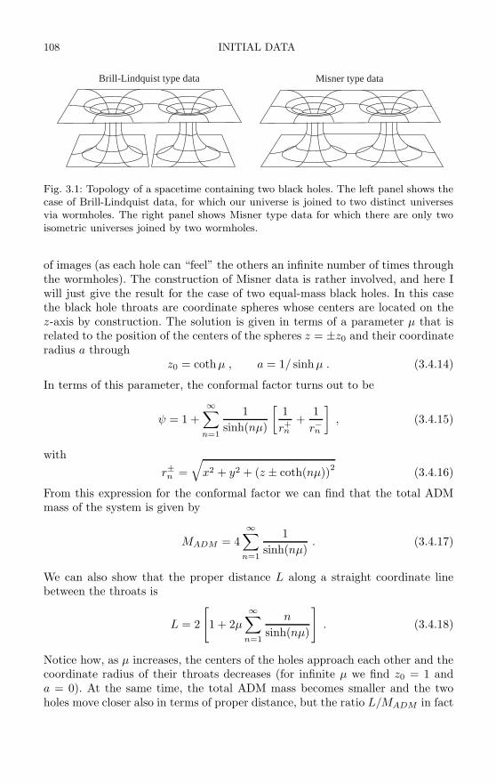
108 INITIAL DATA
Brill-Lindquist type data Misner type data
Fig. 3.1: Topology of a spacetime containing two black holes. The left panel shows thecase of Brill-Lindquist data, for which our universe is joined to two distinct universesvia wormholes. The right panel shows Misner type data for which there are only twoisometric universes joined by two wormholes.
of images (as each hole can “feel” the others an infinite number of times throughthe wormholes). The construction of Misner data is rather involved, and here Iwill just give the result for the case of two equal-mass black holes. In this casethe black hole throats are coordinate spheres whose centers are located on thez-axis by construction. The solution is given in terms of a parameter µ that isrelated to the position of the centers of the spheres z = ±z0 and their coordinateradius a through
z0 = cothµ , a = 1/ sinhµ . (3.4.14)
In terms of this parameter, the conformal factor turns out to be
ψ = 1 +∞∑
n=1
1sinh(nµ)
[1r+n
+1r−n
], (3.4.15)
withr±n =
√x2 + y2 + (z ± coth(nµ))2 (3.4.16)
From this expression for the conformal factor we can find that the total ADMmass of the system is given by
MADM = 4∞∑
n=1
1sinh(nµ)
. (3.4.17)
We can also show that the proper distance L along a straight coordinate linebetween the throats is
L = 2
[1 + 2µ
∞∑n=1
n
sinh(nµ)
]. (3.4.18)
Notice how, as µ increases, the centers of the holes approach each other and thecoordinate radius of their throats decreases (for infinite µ we find z0 = 1 anda = 0). At the same time, the total ADM mass becomes smaller and the twoholes move closer also in terms of proper distance, but the ratio L/MADM in fact
3.4 MULTIPLE BLACK HOLE INITIAL DATA 109
increases. For values of µ less than µ ∼ 1.36 we finds a single apparent horizonaround the two throats [86], while numerical evolutions indicate that for valuesless than µ ∼ 1.8 there is also a common event horizon around the throats onthe initial time slice [23].
Owing to its topological simplicity, for a long time Misner data was consideredmore “natural”. It was frequently used in the numerical simulation of the head-oncollision of two black holes, and as such it has become a reference case. Notice thatprecisely because of the property of having an isometry at each of the wormholethroats, the natural way to evolve Misner type data is to take advantage of theisometry and evolve in 3 minus N balls on which symmetry boundary conditionsare applied. This approach works well in the case of the head-on collision of twoblack holes, where there is rotational symmetry around the axis joining the blackholes and the coordinates can be adapted to the horizons, but it becomes muchmore difficult in the case of orbiting black holes where there are no symmetries,and Cartesian coordinates are used. Because of this, plus the fact that it involvesan infinite number of singular points inside each throat, Misner type initial datais not often used anymore and approaches based on Brill–Lindquist type dataare preferred.
3.4.2 Bowen–York extrinsic curvature
Time-symmetric initial data are a good example of how we can solve the con-straints in simple cases, and are good test cases for numerical codes. Still, theyclearly have no physical relevance because astrophysical black holes would beexpected to have both linear momentum and spin. In this Section we will there-fore consider initial data for moving and spinning black holes, in which case themomentum constraints will no longer be trivial. Remarkably, it turns out thatthere is an analytical solution to the momentum constraints that has the prop-erties we are looking for. Let us start by assuming that we are in vacuum, andalso that the conformal metric is flat γij = δij and the trace of the extrinsiccurvature vanishes K = 0. This last condition is known as that for a maximalslice, as we can show that the volume of a spatial hypersurface for which K = 0is a maximum with respect to small variations.
Consider the momentum constraints in the York–Lichnerowicz conformal de-composition as given by (3.2.19). If we now choose M ij = 0, the constraintsreduce to
∆L V i = D2V i +13
DiDj Vj = 0 . (3.4.19)
It is not difficult to show that this equation has the following solution
V i = − 14r
[7P i + ninjP
j]+
1r2
εijknjSk , (3.4.20)
with P i and Si constant vectors, ni the outward-pointing unit radial vector, andεijk the completely antisymmetric Levi–Civita tensor in three dimensions. To
110 INITIAL DATA
make it more transparent, the last expression can be rewritten in conventionalthree-dimensional vector notation as
V = − 14r
[7P + n (n ·P)] +1r2
n× S . (3.4.21)
Having found the vector V i, the conformal tracefree extrinsic curvature willsimply be given by
Aij =(LV)ij
=3
2r2[niPj + njPi + nkP k (ninj − δij)
]− 3
r3(εilknj + εjlkni)nlSk , (3.4.22)
with Kij = ψ−2Aij (remember that we are taking K = 0). This solution to themomentum constraints is known as the Bowen–York extrinsic curvature [73, 74].
The constant vectors P i and Si have clear physical interpretations. Using theexpressions for the ADM integrals found in Appendix A, we see that the linearand angular momenta at spatial infinity can be calculated as
P i =18π
limr→∞
∮ (Ki
l − δilK)nldS , (3.4.23)
J i =1
16πlim
r→∞
∮εijkxjKkl nldS , (3.4.24)
where the integrals are done over spheres of constant r, with ni the unit outward-pointing normal vector to the sphere, and where the xi are taken to be asymp-totically Cartesian coordinates (notice that in our case K = 0, so the first integralsimplifies somewhat). Assuming now that for large r the conformal factor be-comes unity, and substituting (3.4.22) in the above expressions, we find aftersome algebra that the vectors P i and Si are precisely the linear and angularmomenta for this spacetime. And since the momentum constraints are linear, wecan add solutions of this form at different centers r = ri to represent a set of“particles” with the given momenta and spins.
The Bowen–York extrinsic curvature can be used directly as a solution ofthe momentum constraints, but as it stands it is not isometric when we considerMisner-type initial data. we can, however, find a somewhat more general solutionthat is symmetric with respect to inversions through a coordinate sphere (see [74]for details about the inversion through a sphere). The more general expressionis
Aij =(LV)ij
=3
2r2[niPj + njPi + nkP k (ninj − δij)
]± 3a2
2r4[niPj + njPi − nkP k (5ninj − δij)
]− 3
r3(εilknj + εjlkni)nlSk , (3.4.25)
3.4 MULTIPLE BLACK HOLE INITIAL DATA 111
The extra term proportional to a2 does not contribute to either the linear orangular momenta, but guarantees that the solution is symmetric under inversionthrough a sphere of radius a, the throat of the Einstein–Rosen bridge, whichcan later be identified with the black hole horizon. The two different signs inthe extra term correspond to the cases where the linear momentum on the otherside of the wormhole is either +P i or −P i. When we have more than one blackhole, we can still find solutions that have inversion symmetry with respect toeach throat, but just as before this requires an infinite series expression.
3.4.3 Conformal factor: inversions and punctures
In the last section we found the Bowen–York exact solution to the momentumconstraints that represents a “particle” with a given linear momentum and spin.Of course, in order to complete the initial data specification we still need to solvethe Hamiltonian constraint for the conformal factor ψ. However, the presence of anon-trivial extrinsic curvature implies that we can no longer solve this constraintexactly, so numerical solutions are required.
At this point we have to decide on the type of boundary conditions we willimpose on the solution for the conformal factor. The boundary condition forlarge r comes from the requirement of asymptotic flatness. From our discussionof the Newtonian approximation in Section 1.14, we see that this implies
ψ 1 +M
2r, (3.4.26)
or in differential terms∂rψ =
1r
(1 − ψ) . (3.4.27)
The inner boundary condition is more interesting. Recall that even in thecase of Schwarzschild we found that ψ = 1 + M/2r, which is singular at r = 0.The solution can therefore also be expected to be singular in the more generalcase. There are two different approaches we can take in order to deal with thissingularity.
The first approach is to insist on the inversion symmetry through the throatsof the wormholes using the Bowen–York extrinsic curvature in the form (3.4.25).We then solve the Hamiltonian constraint only on the exterior of the throats,which by construction are fixed at coordinate spheres, using the following bound-ary condition on each of the throats (see Section 6.2)
∂rψ|r=a = − ψ
2r
∣∣∣∣r=a
, (3.4.28)
where r is the coordinate distance to the center of the throat and a is its radius.The inversion method results in data that can be thought of as generalizations
of the Misner type data for the case of non-trivial extrinsic curvature. In fact,this was the first approach used in practice, and resulted in the first initial datasets for orbiting black holes obtained by Cook in the early 1990s [101].

112 INITIAL DATA
The generalization of Brill–Lindquist type initial data was achieved in 1997by Brandt and Bruegmann using what is now known as the puncture method [76].In this case we drop the requirement of inversion symmetry and start from thesimpler form of the Bowen–York extrinsic curvature (3.4.22), adding one termof that type for each black hole. Dropping the inversion symmetry, however,implies that now there are no natural inner boundaries where we can stop theintegration, so we must integrate through the complete 3 interior and deal withthe singularities in the solution for the conformal factor directly.
The basic idea behind the puncture method is to write the conformal factorwith the singular piece explicitly separated as
ψ = ψBL + u , ψBL =N∑
i=1
mi
2 |r − ri| . (3.4.29)
The singular piece is therefore assumed to have the same behavior as in Brill–Lindquist data (but notice that the additive 1 from the Brill-Lindquist conformalfactor (3.4.12) has now been absorbed in the u). It is clear that the term ψBLhas zero Laplacian on 3 with the points r = ri excised, i.e. on a “punctured”3. The Hamiltonian constraint then reduces to
D2flatu + η
(1 +
u
ψBL
)−7= 0 , (3.4.30)
withη =
18ψ7BL
AijAij , (3.4.31)
and we have used the fact that K = 0, and also that the spatial metric isconformally flat so that R = 0. The last equation must now be solved for u.
As before, we must now consider what boundary conditions must be imposedon u, both at infinity and at the punctures. At infinity, asymptotic flatness againimplies that we must have u = 1 + k/r for some constant k, or in differentialform ∂ru = (1 − u)/r.
The key observation of the puncture method is that we can in fact solve foru with no special boundary conditions at the punctures. To see this, notice that,near a given puncture, we have ψBL ∼ 1/|r − ri|, while for Bowen–York extrinsiccurvature of the form (3.4.22) we find that AijA
ij diverges for non-zero spin as|r − ri|−6 and for zero spin as |r − ri|−4, so that η goes to zero as |r − ri| fornon-zero spin and as |r − ri|3 for zero spin. The Hamiltonian constraint thenreduces near the punctures to D2
flatu = 0. Brandt and Bruegmann show thatunder these conditions there exists a unique C2 solution u to the Hamiltonianconstraint in all of 3, so that we can ignore the punctures when solving for u.
Another interesting property of this method is that we can show that eachpuncture corresponds to a separate asymptotically flat region, and that as seenfrom those regions the corresponding black holes have zero linear momentum.This is because the linear momentum on the other side of a given throat arises
3.4 MULTIPLE BLACK HOLE INITIAL DATA 113
through the terms proportional to a2 in (3.4.25), while the puncture methoduses (3.4.22) instead. In fact, we can not use the inversion-symmetric extrin-sic curvature (3.4.25) with this method since in that case we would find thatAijA
ij ∼ |r − ri|−8 near the punctures and η would diverge.We can also show that for puncture type data the ADM masses of the in-
dividual black holes, as calculated on the other asymptotically flat regions, aregiven in terms of the mass parameters mi as
Mi = mi
⎛⎝1 + ui +∑i=j
mj
2rij
⎞⎠ , (3.4.32)
with ui = u(r = ri).The puncture approach is considerably easier to implement numerically than
the inversion-symmetric approach, and because of this in recent years it hasbecome more common in practice.
3.4.4 Kerr–Schild type data
The methods described in the previous section for finding multiple black holedata are very general and can be used to find configurations for multiple blackholes with arbitrary masses, momenta and spins. Still, the basic assumptionsmade, namely K = 0, γij = δij , and an extrinsic curvature of Bowen–York typeimply that we can not generate all possible black hole initial data. In particular, itturns out that while a single Bowen–York black hole with zero linear momentumand zero spin reduces to a Schwarzschild black hole in isotropic coordinates, thecase with zero linear momentum and non-zero spin does not reduce to a Kerrblack hole in any set of coordinates. That this is so can be seen from a result ofGarat and Price that shows that there is no slicing of a Kerr black hole that isaxisymmetric and conformally flat [139].
As it is known that the Kerr solution is the only axisymmetric stationaryblack hole solution, we might wonder what a Bowen–York black hole actuallydescribes, since by construction it is a black hole and it is axisymmetric. Theobvious answer is that a Bowen–York black hole is not stationary, i.e. it is initialdata for a dynamical spacetime that corresponds to Kerr plus some spuriousgravitational waves. In fact, for the particular case of an inversion-symmetricBowen–York black hole, we can explicitly show that it corresponds to a Kerrblack hole plus a Brill wave, that is, a specific type of gravitational wave distor-tion [77, 78]. Something similar is also found for a Bowen–York black hole withlinear momentum and zero spin: It does not correspond to a simple boostedSchwarzschild black hole and contains some spurious gravitational wave contri-bution.
The existence of this spurious gravitational wave content with no clear phys-ical interpretation has led to the search for alternative ways of finding black
114 INITIAL DATA
hole initial data.33 It is important to stress the fact that the problem does notcome from the use of the techniques described in Sections 3.2 and 3.3 whichare completely general, but rather from the specific choices made for the freedata: a maximal initial slice (K = 0) with a conformally flat metric and a purelylongitudinal Bowen–York extrinsic curvature.
Although there has been some work on trying to find alternatives to theBowen–York extrinsic curvature while still retaining a conformally flat metric(see for example [106]), most work has centered around the idea of using Kerrblack holes, originally proposed by Matzner, Huq and Shoemaker [201]. Theproposal calls for the use of superposed boosted Kerr black holes as initial data,but written in Kerr–Schild form to make sure that there are no singularities atthe black hole horizons. Thus, when the black holes are far apart no spuriousgravitational wave content will be present.
Of course, since the Einstein equations are non-linear the principle of super-position is not satisfied, so that we must “correct” this initial data by solvingthe constraints. The method starts by first identifying the 3+1 quantities fromthe Kerr–Schild metric (1.16.16), which turn out to be
α2 =1
1 + 2H, (3.4.33)
βi =2Hli∗
1 + 2H, βi = 2Hli , (3.4.34)
γij = δij + 2Hlilj , γij = δij − 2Hli∗lj∗
(1 − 2H
1 + 2H
), (3.4.35)
with li∗ := δij lj. Now, for a time-symmetric situation we would want the timederivative of the metric to vanish at t = 0. Using this we can find that theextrinsic curvature is given by
Kij =12α
(Diβj + Djβi)
=1√
1 + 2H[∂i (Hlj) + ∂j (Hli) + 2H la∗∂a (Hlilj)] . (3.4.36)
In the particular case of Schwarzschild we have H = M/r and li = xi/r, so thatthe extrinsic curvature becomes
Kij =2M
r4√
1 + 2M/r
[r2δij − xixj (2 + M/r)
]. (3.4.37)
33The total gravitational wave energy content of a single spinning Bowen–York black hole isin fact quite small. Both perturbative and fully non-linear numerical simulations indicate thatfor an angular momentum of J/M2 ∼ 0.5 the energy radiated by such a black hole is of order10−4M [145, 106, 91], which should be compared with ∼ 10−3M for the energy radiated by ahead-on collision of two black holes [28], and ∼ 10−2M for the energy radiated by the inspiralcollision of two orbiting black holes [42, 43].

3.5 BINARY BLACK HOLES IN QUASI-CIRCULAR ORBITS 115
If, on the other hand, we want to have a black hole with some initial linearmomenta, we can use instead a boosted Schwarzschild or Kerr black hole asstarting point and compute the corresponding extrinsic curvature.
In order to find binary black hole initial data we now choose the conformalmetric γij as a direct superposition of two Kerr–Schild metrics
γijdxidxj =[δij + 2H(1)(r1) l
(1)i l
(1)j + 2H(2)(r2) l
(2)i l
(2)j
]dxidxj , (3.4.38)
where H(a) and l(a)i are the functions corresponding to a single black hole. As
before, the physical metric will be related to this metric by γij = ψ4γij , and wewould need to solve the Hamiltonian constraint to find ψ.
For the momentum constraints, we take as a trial extrinsic curvature simplythe direct sum of the extrinsic curvatures for the two Kerr–Schild black holes. Wethen take the trace of the resulting extrinsic curvature as K, and the tracefreepart as M ij , and solve the momentum constraints using the techniques describedin Section 3.2 to find the physical extrinsic curvature.
Since the work of Matzner et al., other approaches based on the idea ofusing Kerr–Schild data as a starting point have also been proposed [58, 210]. Wemight expect that these approaches would result in smaller amounts of spuriousgravitational waves than the Bowen–York approach. Kerr–Schild initial data forbinary black hole collisions have in fact been used in practice, though their totalcontent of gravitational waves has not yet been estimated.
3.5 Binary black holes in quasi-circular orbits
Perhaps the most important motivation for constructing multiple black hole ini-tial data is the study of the inspiral coalescence of binary black holes. This is thesimplest form of the two body problem in general relativity, which is well knownto have no solution in closed form. The reason for this is easy to understand: Asthe black holes orbit each other they continually radiate gravitational waves. Asa result of this the system loses energy and the black holes spiral in, orbitingfaster and faster until they eventually collide and merge.
To study this problem numerically, we would first need to find initial datafor a binary system of black holes in quasi-circular orbits. This is because theemission of gravitational waves is expected to circularize an initially ellipticalorbit in time-scales much shorter than the merger time-scale. To date, there arebasically two approaches for constructing quasi-circular initial data for binaryblack holes. The first approach was introduced in the early 1990s and is based onthe idea of minimizing a measure of the total energy of the binary while keepingthe total angular momentum fixed. This approach is known to result in circularorbits in the case of Newtonian gravity, and is therefore expected to producequasi-circular orbits in the general relativistic case. The second approach wasproposed by Grandclement et al. in 2001 and is based on the idea of lookingfor solutions in quasi-equilibrium, for which an approximate Killing field exists.
116 INITIAL DATA
Below we will briefly discuss each of these two approaches to finding initial datafor black holes in quasi-circular orbits.
3.5.1 Effective potential method
As already mentioned, the effective potential method is based on the fact thatminimizing the total energy of a binary system in Newtonian gravity, while keep-ing the total angular momentum fixed, results in circular orbits. The problemwith applying this idea to the case of general relativity is twofold. First, it isclear that we can not find perfectly circular orbits since the black holes will ra-diate gravitational waves. However, we would expect that for a system that isnot too close to the final plunge phase the time-scale for energy loss due to grav-itational wave emission will be considerably larger than the orbital time-scale.The second problem has to do with the definition of the energy of the system ingeneral relativity. Notice that although a measure of the total energy content ofthe spacetime can in fact be found in terms of the ADM mass as described inAppendix A, this total energy includes both the gravitational “binding energy”of the system and the mass energy of the individual black holes. We must clearlyonly minimize the effective potential energy defined as
Eb := MADM − M1 − M2 , (3.5.1)
where MADM is the ADM mass of the full spacetime, and Mi are the individualmasses of each black hole. The basic problem here is how to define the massesof the individual black holes, as these are not well-defined concepts for blackholes that are close to each other. The usual approach is to use the relationshipbetween the area of the horizon A and the mass M of a single Kerr black hole
M2 = M2I + S2/4M2
I = A/16π + 4πS2/A , (3.5.2)
where MI =√
A/16π is the irreducible mass and S is the spin of the black hole.In order to find quasi-circular orbits we then have to fix the spin Si and
horizon areas Ai of the individual black holes so that their total masses remainconstant, fix also the total angular momentum of the spacetime J , and thenminimize the binding energy as a function of the separation L between the blackhole horizons. In practice we must move the black holes to a certain separation,locate the individual horizons (see Chapter 6) and adjust the parameters of thefree data until the physical parameters Si, Ai and J reach the desired values.After that, we compute the ADM mass MADM for that separation and startagain at a different separation until we find a minimum.
Quasi-circular data using the effective potential method, together with anextrinsic curvature of the Bowen–York type, were computed for isometric databy Cook [101], and later for puncture data by Baumgarte [49], with very similarresults found in both cases. As we decrease the total angular momentum of thesystem, the minimum in the binding energy becomes shallower and is found atprogressively closer separations. At a certain critical separation the minimum

3.5 BINARY BLACK HOLES IN QUASI-CIRCULAR ORBITS 117
disappears altogether so that no quasi-circular orbit is found. This critical sepa-ration is known as the innermost stable circular orbit (ISCO), and if the holes arecloser than this they will stop orbiting and will just plunge toward each other.34
For non-spinning equal-mass black holes, Cook finds the ISCO at a proper sep-aration between the black hole horizons of L/m ∼ 4.88, with m = 2M and Mthe mass parameter of the individual black holes, corresponding to a coordinateseparation between the black hole centers of D/m ∼ 2.2. The two black holeshave equal and opposite linear momenta given by P/m ∼ 0.33, and the totalangular momentum of the system is J/m2 ∼ 0.74. The angular velocity can alsobe estimated using
Ω =∂Eb
∂J, (3.5.3)
which for the ISCO results in mΩ ∼ 0.17. A table of parameters for quasi-circularorbits scaled in terms of the ADM mass of the system can be found in [43].
The use of the effective potential method together with Bowen–York extrinsiccurvature can only be expected to be a good approximation for large separations,so the position of the ISCO found with this method should not be trusted. Indeed,numerical simulations of this ISCO show that the black holes do not orbit andinstead rapidly plunge toward each other [42, 11]. However, the quasi-circularorbit estimations should rapidly improve as the separation is increased.
3.5.2 The quasi-equilibrium method
As mentioned above, the effective potential method coupled to the use of extrinsiccurvature of the Bowen–York type provides us with initial data that are a goodapproximation to black holes in quasi-circular orbit at large separations, but thedata can not be trusted for separations close to the ISCO.
Recently, an alternative method for finding initial data for black holes inquasi-circular orbits has been proposed by Grandclement et al. [150], based onan approach that has been used very successfully in the past to construct initialdata for orbiting neutron stars. The basic idea is that for sufficiently separatedblack holes the spacetime can be supposed to be quasi-stationary, which meansthat there should exist an approximate helical Killing field ξ. We can then usethis idea to construct initial data for which the conformal 3-geometry remainsmomentarily constant. Notice that, in order to do this consistently, we need tobe on a coordinate frame corotating with the black holes. Since the idea is basedon trying to reduce as much as possible the rate of change of the conformalmetric, the natural framework for this approach is the conformal thin-sandwichformalism described in Section 3.3.
34The ISCO also exists for a test particle orbiting a Schwarzschild black hole, and in thatcase it is found at an areal radius of r = 6M , corresponding to a proper distance betweenthe black hole horizon and the test mass of ∼ 4.58. This shows a very important differencebetween general relativity and Newton’s theory for which circular orbits exist arbitrarily closeto a point mass.

118 INITIAL DATA
Let us then start from the standard conformal decomposition of the met-ric γij = ψ−4γij . We will now assume that the initial conformal metric is flatγij = δij , and also that we start from a maximal slice K = 0. Since we wantquasi-stationary initial data, it is natural to ask for
uij := ∂tγij = 0 , ∂tK = 0 . (3.5.4)
Notice that with these choices we have now completely exhausted the free datafor the conformal thin-sandwich method. In particular, the previous choices willfix the lapse and shift through equations (3.3.9) and (3.3.18).
Even though by construction we will have momentarily stationary values forthe conformal metric and extrinsic curvature, in general we will not have ∂tψ = 0or ∂tAij = 0. This is where the existence of an approximate Killing field comesinto play. It implies that it should be possible to choose coordinates such that∂tψ ∼ 0 and ∂tAij ∼ 0. Of course, as already mentioned the lapse and shifthave already been fixed by our previous choices, but only up to the boundaryconditions used for the elliptic equations.
Consider the boundary conditions at infinity. Asymptotic flatness impliesthat the lapse must be such that limr→∞ α = 1. The shift, however, is moreinteresting. As already mentioned it is clear that if want to minimize changes inthe geometry we must go to a corotating frame, so that far away the shift vectormust approach a rigid rotation:
limr→∞
β = Ω eφ , (3.5.5)
where eφ is the basis vector associated with the azimuthal angle φ.At this point, however, we still don’t have information that will allow us to
fix the angular velocity Ω. Grandclement et al. suggest that this can be doneby comparing two different definitions of the mass of the spacetime, namely theADM mass and the Komar mass. As discussed in Appendix A, the total mass andangular momentum at spatial infinity can be expressed via the ADM integrals:
MADM =1
16πlim
r→∞
∮γij [γik,j − γij,k]dSk , (3.5.6)
JADM =18π
limr→∞
∮Kijeφ
idSj , (3.5.7)
where the integrals are taken over coordinate spheres, and where dSi = sidAwith si the unit outward-pointing normal vector to the sphere (in the first in-tegral above, the spatial metric must be expressed in asymptotically Cartesiancoordinates). In the particular case of a conformally flat spatial metric like theone we are using here, the first integral can be shown to reduce to
MADM = − 12π
limr→∞
∮∂iψ dSi . (3.5.8)
3.5 BINARY BLACK HOLES IN QUASI-CIRCULAR ORBITS 119
Now, in the case when the spacetime admits a Killing field ξ, we can alsodefine conserved quantities through the Komar integral (remember that for aKilling field we have ∇(µξν) = 0):
IK
(ξ)
= − 14π
∮sµnν∇µξν dA , (3.5.9)
where here nµ is the timelike unit normal to the spacelike hypersurfaces. If ξµ istimelike and such that ξµξµ = 1 at infinity, then the above integral correspondsto the total mass of the spacetime M , while if it is an axial vector associatedwith an angular coordinate φ it will correspond to −2J , with J the total angularmomentum (the factor −2 is needed to obtain the correct normalization). TheKomar mass and angular momentum should coincide with the ADM integrals.
In our case we have neither a timelike nor an axial Killing field, but we dohave an (approximate) helical Killing field. If we choose the boundary conditionson the shift appropriately, this Killing field should correspond to the time vectorξµ = tµ = αnµ + βµ, and we would expect the following relation to hold [290]
Ik
(αn + β
)= MADM − 2ΩJADM , (3.5.10)
where the factor Ω appears because far away β = Ωeφ. Notice now that
sµnν∇µξν = sµnν (α∇µnν + nν∇µα + ∇µβν) . (3.5.11)
Using the fact that nµnµ = −1 and nµβµ = 0 we can rewrite this as
sµnν∇µξν = sµ (−∇µα − βν∇µnν) = −sµ (∇µα − βνKµν) . (3.5.12)
The Komar integral then becomes
IK
(ξ)
=14π
∮ (∇kα − βjKjk
)dSk
=14π
∮∇kα dSk − Ω
4π
∮Kjkeφ
j dSk . (3.5.13)
Comparing the last result with the ADM expressions given above, we see thatthe angular momentum part is identical while the mass part differs, being givenin the Komar case in terms of the lapse α and in the ADM case in terms of theconformal factor ψ. The relation (3.5.10) then reduces to∮
∇kα dSk = −2∮
∇kψ dSk . (3.5.14)
The last condition must hold if tµ = αnµ +βµ is a Killing vector, but for thisto be the case we must know the correct angular velocity in order to have theshift correspond to a true corotation frame. The key observation here is that we

120 INITIAL DATA
can turn the condition around and use it to determine the angular velocity. Theidea is to solve the conformal thin-sandwich equations with a given value of Ωfixing the exterior boundary condition for the shift, and then change the value ofΩ until (3.5.14) is satisfied. Of course, in our case we only have an approximateKilling field, but we would expect that this way of fixing the angular velocitywill still bring us to the correct corotating frame. Notice that for Schwarzschildthe asymptotic behavior of the lapse and the conformal factor is
ψ 1 + M/2r , α 1 − M/r , (3.5.15)
which is precisely of the form (3.5.14). In the more general case we will stillhave ψ 1 + Mψ/2r and α 1 − Mα/r, but Mψ and Mα can not be expectedto coincide unless we use the correct angular velocity for the shift boundarycondition. This is the fundamental element of the quasi-equilibrium approach.
Of course, we still need to worry about the inner boundary conditions eitherat the black hole horizons or at the punctures. This issue is very technical andwe will not discuss it in detail here. However, it should be mentioned that inthe original approach of Grandclement et al. the initial data is assumed to beinversion-symmetric at the black hole throats, which also correspond to apparenthorizons, a condition that requires the black holes to be corotating (i.e. their spinis locked with the orbital motion). However, as pointed out by Cook [103], thisset of boundary conditions does not guarantee regularity, and when an artificialregularization procedure is used it leads to solutions that no longer satisfy theconstraints near the throats. In [103] Cook has generalized the original proposalto allow for regular boundary conditions by giving up the inversion symmetry,and has thus been able to obtain solutions for black holes that can have arbitraryspins. Tichy et al. have also applied the quasi-stationary idea to puncture typedata with Bowen–York extrinsic curvature [289, 290].
As a final note it is important to mention that very recently Caudill et al.have shown that, when using the conformal thin-sandwich approach, the effectivepotential method and the Komar mass method give results that are remarkablyclose to each other [95]. The main differences between the quasi-equilibrium andthe puncture approaches should therefore be attributed to the use of the Bowen–York extrinsic curvature and not to the effective potential method itself.
4
GAUGE CONDITIONS
4.1 Introduction
As already mentioned in Chapter 2, in the 3+1 formalism the choice of thecoordinate system is given in terms of the gauge variables: the lapse function αand the shift vector βi. These functions appear in the evolution equations (2.3.11)and (2.5.5) for the metric and extrinsic curvature. However, Einstein’s equationssay nothing about how the gauge variables should be chosen. This is what shouldbe expected, since it is clear that the coordinates can be chosen freely.
The freedom in choosing the gauge variables is a mixed blessing. On the onehand, it allows us to choose the coordinates in a way that either simplifies theevolution equations or makes the solution better behaved. On the other hand,we are immediately faced with the following question: What is a “good” choicefor the functions α and βi?
There are, of course, some guidelines that one would like to follow whenchoosing good gauge conditions, which can be summarized in the following “wishlist”:
• Whenever possible, gauge conditions should be adapted to the underlyingsymmetries of the problem. Ideally the gauge conditions should automati-cally “seek” exact or approximate symmetries of the spacetime and makethem evident in the evolution.
• The gauge conditions should avoid the formation of coordinate singulari-ties. In the case of black hole spacetimes, they should also avoid reachingthe physical singularity.
• Gauge conditions should be well behaved mathematically, and wheneverpossible easy to implement numerically.
• Ideally, gauge conditions should be expressed in 3-covariant form, this willguarantee that we will have the same gauge when using different spatialcoordinate systems (e.g. Cartesian vs. spherical).
In order to find gauge conditions with these properties, the natural approachis to relate the gauge choice to the evolution of certain combinations of geometricquantities in such a way that the gauge will either freeze completely the evolutionof those quantities (typically by solving some elliptic equations), or will attemptto do so with some time delay (by solving parabolic or hyperbolic equations in-stead). Below I will describe the most common gauge conditions used in practicein numerical relativity.
121

122 GAUGE CONDITIONS
4.2 Slicing conditions
In order to specify a foliation of spacetime into spacelike hypersurfaces, alsoknown as a synchronization, we need to prescribe a way to calculate the lapsefunction α which measures the proper time interval between neighboring hyper-surfaces along the normal direction.
Typically, the different possible lapse choices can be classified in the followingway: 1) Prescribed slicing conditions where the lapse is specified as an a prioriknown function of space and time, 2) algebraic slicing conditions where thelapse is specified as some algebraic function of the geometric variables at eachhyper-surface, 3) evolution-type slicing conditions where the time derivative ofthe lapse is specified as an algebraic function of the geometric variables andthe lapse is evolved as just another dynamical quantity, and 4) elliptic slicingconditions where the lapse is obtained by solving an elliptic differential equationat every time step that typically enforces some geometric condition on the spatialhypersurfaces.
Before considering different slicing conditions we must mention a couple ofresults that are very important when discussing this issue. First, consider themotion of the Eulerian (normal) observers. There is no reason to assume thatthese observers will be in free fall, so in general they should have a properacceleration that measures the force that would be required to keep them ina trajectory different from free fall. This acceleration is given in terms of thedirectional derivative of the 4-velocity of the Eulerian observers, i.e. the normalvector nµ, along itself:
aµ = nν∇νnµ . (4.2.1)
Notice first that nµaµ = nµnν∇νnµ = 0, i.e the vector aµ is orthogonal to nµ (asexpected since nµ is unitary), so the proper acceleration is a purely spatial vector.Using now the expressions for nµ in terms of α and βi given in equation (2.2.8),and the expressions for the 4-Christoffel symbols found in Appendix B, we caneasily show that
a0 = βm∂m ln α , (4.2.2)ai = ∂i ln α . (4.2.3)
We then see that the spatial components of the proper acceleration are given bythe gradient of the lapse.
Another important relationship comes from the evolution of the volume ele-ments associated with the Eulerian observers. The change in time of these volumeelements is simply given by the divergence of their 4-velocities ∇µnµ. Using nowthe definition of the extrinsic curvature we find that:
∇µnµ = −K , (4.2.4)
that is, the rate of change of the volume elements in time is just (minus) thetrace of the extrinsic curvature.
4.2 SLICING CONDITIONS 123
4.2.1 Geodesic slicing and focusing
The most obvious way to choose the lapse function would be to ask for thecoordinate time t to coincide everywhere with the proper time of the Eulerianobservers, that is α = 1. After all, what could be more natural? This is an exam-ple of a prescribed slicing condition and is known as geodesic slicing. The namecomes from the fact that according to equation (4.2.3) the proper accelerationof the Eulerian observers vanishes for constant α, which implies that in this casethe Eulerian observers follow timelike geodesics (i.e. they are in free fall).
Geodesic slicing was in fact used in the pioneering work of Hahn and Lindquistin the mid 1960s [158]. However, it is now well known that geodesic slicing is avery poor coordinate choice. The reason for this is easy to see if we think fora moment about what will happen to observers in free fall in a non-uniformgravitational field. As the field is non-uniform, different observers will fall in dif-ferent directions, and nothing can prevent them from eventually colliding withone another. When this happens, our coordinate system (which is tied to theseobservers) stops being one-to-one: One point has now more than one set of co-ordinates associated with it. This means that the coordinate system has becomesingular.
In order to see this, consider the evolution equation for the trace of theextrinsic curvature. From the ADM evolution equations (2.3.12) and (2.5.6) wefind that
∂tK = βi∂iK − D2α + α[KijK
ij + 4π (ρ + S)]
, (4.2.5)
where we have used the Hamiltonian constraint (2.4.10) to eliminate the Ricciscalar. For geodesic slicing this equation reduces to
∂tK − βi∂iK = α[KijK
ij + 4π (ρ + S)]
. (4.2.6)
The first term on the right hand side is clearly always positive, and so is thesecond term if the strong energy condition holds. This means that along thenormal direction the trace of the extrinsic curvature K will increase withoutbound, which through (4.2.4) implies that the volume elements associated withthe Eulerian observers will collapse to zero. Because of this, geodesic slicing isnever used in practice except to test numerical codes. For example, it is wellknown that the free fall time to the singularity for an observer initially at restat the Schwarzschild horizon is t = πM . We can then set up initial data forSchwarzschild in isotropic coordinates, evolve using geodesic slicing, and expectthe code to crash at that time.
4.2.2 Maximal slicing
In order to look for a better slicing condition, we must think about what preciselywas wrong with geodesic slicing. The main problem was that observers in free fallare “focused” by the gravitational field. This means that they will get closer toeach other, so the volume elements associated with them will become smaller andsmaller until they become zero. We can then try to built a better slicing condition
124 GAUGE CONDITIONS
by demanding that the volume elements associated with the Eulerian observersremain constant. From equation (4.2.4) we can see that this is equivalent toasking for
K = ∂tK = 0 . (4.2.7)
It is clear that we must require not only that K vanishes initially, but also thatit remains zero during the evolution. Asking now for the above condition to hold,we find through (4.2.5) that the lapse function must satisfy the following ellipticequation
D2α = α[KijK
ij + 4π (ρ + S)]
. (4.2.8)
This condition is known as maximal slicing.35 The name comes from the factthat we can prove that when K = 0 the volume of the spatial hypersurface ismaximal with respect to small variations in the hypersurface itself.
Maximal slicing was suggested originally by Lichnerowicz [189], and was al-ready discussed in the classic papers of Smarr and York [272, 305]. It has beenused over the years for many numerical simulations of a number of different sys-tems, including black holes, and is still in use today. It has the advantage ofbeing given by a simple equation whose solution is smooth (because it comesfrom an elliptic equation), and also of guaranteeing that the Eulerian observerswill not focus. It is important to mention also that this slicing condition canonly be used for asymptotically flat spacetimes and can not be used in the caseof cosmological spacetimes where volume elements always expand or contractwith time (on a closed Universe only one maximal slice exists at the momentof time symmetry). However, in that case we can relax the condition and useK = constant, with a different constant for each slice (in fact, in such cases Kcan be used as a time coordinate). For asymptotically flat spacetimes we can infact also use the condition K = K0 = constant, ∂tK = 0. This corresponds tohyperboloidal slices that reach null infinity J ± (depending on the sign of K0).Such hyperboloidal slices can be useful to study gravitational radiation at infin-ity, and are natural choices in Friedrich’s conformal approach (see Section 2.9.2).They have also been used in numerical simulations based on the standard 3+1approach to improve the stability of the evolution [142].
A very important property of maximal slicing is that of singularity avoidance,by which we mean that it does not allow the spatial hypersurfaces to come arbi-trarily close to a physical singularity. In the particular case of the Schwarzschildspacetime the maximal slices can be constructed analytically (see the followingSection), and it is well known that inside the horizon the maximal slices approacha limiting surface given by r = 3M/2, with r the Schwarzschild areal radius (re-member that inside the horizon the hypersurfaces r = constant are spacelike), so
35Maximal slicing is given by an elliptic equation similar to the Helmholtz equation, whichin standard 3D vector notation is ∇2φ+ k2φ = 0. However, since as long as the strong energycondition holds we have KijKij + 4π(ρ + S) ≥ 0, the sign of the source term in the maximalslicing equation is opposite to that of the standard Helmholtz equation.
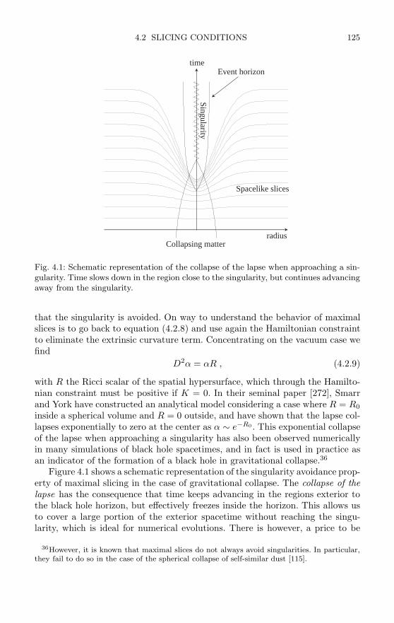
4.2 SLICING CONDITIONS 125
Collapsing matter
Spacelike slices
time
radius
Event horizon
Singularity
Fig. 4.1: Schematic representation of the collapse of the lapse when approaching a sin-gularity. Time slows down in the region close to the singularity, but continues advancingaway from the singularity.
that the singularity is avoided. On way to understand the behavior of maximalslices is to go back to equation (4.2.8) and use again the Hamiltonian constraintto eliminate the extrinsic curvature term. Concentrating on the vacuum case wefind
D2α = αR , (4.2.9)
with R the Ricci scalar of the spatial hypersurface, which through the Hamilto-nian constraint must be positive if K = 0. In their seminal paper [272], Smarrand York have constructed an analytical model considering a case where R = R0inside a spherical volume and R = 0 outside, and have shown that the lapse col-lapses exponentially to zero at the center as α ∼ e−R0 . This exponential collapseof the lapse when approaching a singularity has also been observed numericallyin many simulations of black hole spacetimes, and in fact is used in practice asan indicator of the formation of a black hole in gravitational collapse.36
Figure 4.1 shows a schematic representation of the singularity avoidance prop-erty of maximal slicing in the case of gravitational collapse. The collapse of thelapse has the consequence that time keeps advancing in the regions exterior tothe black hole horizon, but effectively freezes inside the horizon. This allows usto cover a large portion of the exterior spacetime without reaching the singu-larity, which is ideal for numerical evolutions. There is however, a price to be
36However, it is known that maximal slices do not always avoid singularities. In particular,they fail to do so in the case of the spherical collapse of self-similar dust [115].

126 GAUGE CONDITIONS
paid. As time advances outside and freezes inside, the spatial slices become moreand more distorted, leading to a phenomenon known as slice stretching whichresults in a rapid growth of the radial metric component and the developmentof large gradients, which eventually cause numerical codes to fail.37 As pointedout by Reimann in [237, 236], slice stretching is in fact a combination of two sep-arate effects, referred to by Reimann as slice sucking and slice wrapping. Slicesucking refers to the fact that the mere presence of the black hole results in thedifferential infall of coordinate observers, as those closer to the black hole fallfaster, resulting in their radial separations increasing and the radial metric com-ponent growing. This means that slice stretching will occur even for geodesicslicing. The second effect of slice wrapping is the one that one usually has inmind when thinking about singularity avoidance and is precisely a consequenceof the collapse of the lapse and the slices “wrapping” around the singularity.Slice stretching results in a power law growth of the radial metric. For the max-imal slicing of Schwarzschild, Reimann finds that at late times the peak in theradial metric grows as ∼ τ4/3, with τ proper time at infinity (the loose statementoften found in the numerical literature indicating that slice stretching results in“exponential” growth of the radial metric is therefore incorrect).
If there is a major disadvantage to maximal slicing it is the fact that solvingelliptic equations numerically in three dimensions is a very slow process. Evenwith fast elliptic solvers, we can find that over 90% of the processor time is usedto solve just the maximal slicing equation (with zero shift; if we also have ellipticshift conditions things get much worse). Also, setting up boundary conditionsfor complicated inner boundaries such as those that can be found when excisingblack hole interiors (see Chapter 6) can be a very hard problem. Because of thisin the past few years maximal slicing has been giving place to hyperbolic-typeslicing conditions like those that we will discuss in Section 4.2.4. Still, whencomputer time restrictions are not an issue and good boundary conditions areknown, maximal slicing is probably the best slicing condition available.
Since maximal slicing requires the solution of an elliptic problem, the issueof boundary conditions is very important (here I will consider only the exteriorboundaries and ignore the possible presence of complicated interior boundaries).For asymptotically flat spacetimes we can assume that far from the sources weshould approach the Schwarzschild solution, in which case the lapse functionbehaves asymptotically as
α = 1 − c/r , (4.2.10)
with c some constant (in static coordinates we find c = M) . We can eliminatethe unknown constant by taking a derivative with respect to r to find
∂rα = (1 − α) /r . (4.2.11)
37In older literature one often finds that this is called grid stretching, but the name ismisleading as this is a geometric effect that happens at the continuum level, and is quiteindependent of the existence of a numerical grid.

4.2 SLICING CONDITIONS 127
This is known as a Robin boundary condition and is the standard condition usedwhen solving maximal slicing.
4.2.3 Maximal slices of Schwarzschild
In the case of a Schwarzschild black hole, the maximal slicing equation can infact be solved analytically [51, 52, 126, 224, 238, 239]. This allows us to under-stand many of the properties of this slicing in detail, and even make quantitativestatements about the late time behavior of the lapse. In the discussion presentedhere I will follow closely the work of Beig and O’Murchadha [51, 52] (there areother ways to derive the same results – in particular Estabrook et al. take adifferent route that starts from the constraint equations [126]). We start fromthe Schwarzschild metric in standard Schwarzschild coordinates:
ds2 = −(
1 − 2M
r
)dt2 +
(1 − 2M
r
)−1dr2 + r2dΩ2 . (4.2.12)
Consider for a moment a hypersurface r = constant. We know that for r < 2Mthese hypersurfaces will be spacelike. The trace of the extrinsic curvature Kfor such a hypersurface can be easily obtained. By taking t to be a space co-ordinate and r to be the time coordinate (but moving backwards as r becomessmaller with proper time), the spatial volume elements are found to be given byγ = r4 sin2 θ (2M/r − 1) and the lapse function becomes α = 1/
√2M/r − 1. In
that case K can be found through the ADM equations by
d
drln γ = 2αK ⇒ K =
3M − 2r
r2√
2M/r − 1. (4.2.13)
Notice that here r is taken to be constant, so K is the same along the slice.In particular, we see that the hypersurface r = 3M/2 is a maximal slice. Wewill see below that this will be the limiting slice for the maximal foliation ofSchwarzschild.
Consider now some arbitrary spherically symmetric spatial hypersurface inthe Schwarzschild spacetime given as
σ(t, r) = t − F (r) = constant ⇒ t = F (r) + σ . (4.2.14)
Let us now construct the normal vector nµ to this hypersurface
nµ = −N ∇µσ = −N (1,−F ′) , (4.2.15)
with F ′ := dF/dr, and where N is a normalization coefficient fixed by asking fornµ to be a unit vector
nµnµ = N2
[−(
1 − 2M
r
)−1+(
1 − 2M
r
)F ′2]
= −1 . (4.2.16)
Solving the last equation for F ′ we find
128 GAUGE CONDITIONS
F ′2 =(
1 − 2M
r
)−2− 1
N2
(1 − 2M
r
)−1. (4.2.17)
Let us now ask for our slice to be maximal, that is
K = −∇µnµ = − 1|g|1/2 ∂µ
(|g|1/2nµ
)= 0 . (4.2.18)
Using the Schwarzschild metric above and the expression for nµ we find
0 =1r2
∂r
[r2NF ′
(1 − 2M
r
)]⇒ r2NF ′
(1 − 2M
r
)= C , (4.2.19)
with C some constant (C is often called the Estabrook–Wahlquist time as it canbe used to parameterize the different slices [126]). Inserting now the expressionfor F ′ in the equation above and solving for N we find
N =1r2(r4 − 2Mr3 + C2
)1/2. (4.2.20)
And substituting this back into the expression for F ′ we finally find
F ′ = ± C
(1 − 2M/r)(r4 − 2Mr3 + C2)1/2. (4.2.21)
There are a couple of comments to be made here before proceeding anyfurther. First, consider the sign in the previous expression. As we have seen, thetimelike normal vector is given by nµ = −N (1,−F ′), with N > 0. For r > 2Mthe coordinate t is timelike, and the vector nµ will clearly be future pointingregardless of the sign of F ′. For r < 2M , however, the timelike coordinate isnow r, and r becomes smaller to the future, so that in order for nµ to be futurepointing we must ask for nr > 0, that is F ′ > 0. We therefore take the minussign in the expression for F ′ above.
The second point has to do with the fact that we are looking for slices thatdo not reach the singularity at r = 0. That is, as seen in the Kruskal diagram,we want slices that come in from infinity, reach a minimum value of r at thethroat of the Einstein–Rosen bridge, and then go back to infinity on the otherasymptotically flat region. At the throat the slices should in fact be tangential toa surface r = constant, so that dt/dr = F ′ becomes infinite. Looking at (4.2.21),we see that F ′ becomes infinite both at the horizon r = 2M and at any root ofthe quartic polynomial
P (r) = r4 − 2Mr3 + C2 . (4.2.22)
As we will see below, at r = 2M the infinite value of F ′ is related to the singular-ity of the Schwarzschild coordinates, and the slices in fact go smoothly throughthe horizon. We then conclude that we must have a non-trivial real root of P (r)if we want to obtain slices that do not reach the singularity at r = 0. Looking

4.2 SLICING CONDITIONS 129
at the form of the polynomial P (r) it is not difficult to show that there will betwo distinct real roots for C2 < 27M4/16 (both roots are such that r > 0), andno roots if C2 exceeds this value.38 We will therefore ask for C2 < 27M4/16.Define now rC as the position of the largest real root of P (r). The particularcase C2 = 0 corresponds to rC = 2M and in fact reduces to the Schwarzschildt = 0 slice (or t = constant for a non-zero value of σ). On the other hand, as C2
approaches the critical value 27M4/16, rC becomes smaller and approaches thevalue 3M/2 corresponding to the limiting maximal slice of Schwarzschild.
The function F will now be given by integrating (4.2.21):
F (r, C) = −∫ r
rC
C
(1 − 2M/x) [P (x)]1/2dx , (4.2.23)
where the integral over the pole at x = 2M is taken in the sense of the principalvalue. In order to see that the surfaces are indeed smooth at r = 2M , define first
H(r, C) := F (r, C) + 2M ln (r/2M − 1) . (4.2.24)
This implies thatdH
dr= −Cr − 2M [P (r)]1/2
(r − 2M) [P (r)]1/2. (4.2.25)
Taking now the limit of the last expression when r approaches 2M we find
limr→2M
dH
dr=
8M4
C2− 1 . (4.2.26)
That is, H(r, C) is a smooth function of r at the horizon. But notice now that
H(r, C) = t − σ + 2M ln (1 − r/2M) = t − σ , (4.2.27)
with t = t+2M ln (1 − r/2M), the Eddington–Finkelstein time used to transformthe Schwarzschild metric to the regular Kerr–Schild form (1.15.20). We then findthat in terms of the regular coordinate t, the slices defined above cross the horizonsmoothly.
Let us now go back to the expression for F (r, C), equation (4.2.23). Thereare two ways we can use this to derive a maximal foliation of the Schwarzschildspacetime. The first is to simply take C = 0 in which case the foliation re-duces to t = σ = constant, so that we recover the standard Schwarzschild slices(which are of course maximal since the metric is time independent and the shiftvector vanishes, which implies Kij = 0). We call these the odd maximal slicesof Schwarzschild since they correspond to the lapse going to 1 at one of theasymptotically flat regions and to −1 at the other asymptotically flat region.
38Notice that since there are two roots with r > 0, we in fact have two families of solutions,one from r = 0 to the left root, and another from the right root to r = ∞. The first family willclearly reach the singularity at r = 0 so we are not interested in it.

130 GAUGE CONDITIONS
A more interesting situation is obtained by varying the value of C, startingfrom 0 and reaching the limiting value Clim = 3
√3M2/4. In this case we take
σ = 0 since changing the value of σ will give us precisely the same foliation onlystarting at a different value of the Schwarzschild time t. Instead of parameterizingthese slices with the value of the constant C, we will use as parameter the propertime measured at infinity, which is clearly given by
τ(C) = F (∞, C) = −∫ ∞
rC
C
(1 − 2M/x) [P (x)]1/2dx . (4.2.28)
The lapse function α associated with this foliation is then defined through
nµ = −α∇µτ . (4.2.29)
Notice now that et ·n = nt = −N , with et the coordinate basis vector associatedwith t, and also that et · ∇τ = ∂τ/∂t. This implies
N = α∂τ
∂t. (4.2.30)
Solving for α we find
α = N∂t
∂τ= N
∂F
∂τ= N
∂F
∂C
dC
dτ. (4.2.31)
The problem now is to find ∂F/∂C, which is a non-trivial task. To see why thisis so, notice that the lower limit of integration in (4.2.23) is rC which clearlydepends on C. We therefore pick up a boundary term when differentiating withrespect to C, given essentially by the integrand itself evaluated at rC , whichclearly diverges (remember that rC is a root of P (r)). There is, however, a trickthat can be used to calculate this derivative (the derivation is rather long so wewill not include it here; the interested reader can see Appendix B of [51]). Wefind that
∂F (r, C)∂C
=r2
2 (r − 3M/2)P (r)1/2− 1
2
∫ r
rC
x (x − 3M)(x − 3M/2)2 P (x)1/2
dx . (4.2.32)
Using now the expression for N , the lapse finally becomes
α =12
dC
dτ
[1
r − 3M/2− P (r)1/2
r2
∫ r
rC
x (x − 3M)(x − 3M/2)2 P (x)1/2
dx
]. (4.2.33)
Notice that this expression is regular at r = rC . We can in fact also show thatboth α and N are linearly independent spherically symmetric solutions of themaximal slicing equation (D2 − KijK
ij)f = 0, but with different boundaryconditions: Both N and α go to 1 at the right infinity, but at the left infinity Ngoes to −1 while α goes to 1.

4.2 SLICING CONDITIONS 131
We can now use expression (4.2.33) to study the late time behavior of thelapse at different interesting locations. Notice first that, as C goes to Clim =3√
3M2/4, τ(C) goes to infinity and the areal radius r goes to 3M/2. Definenow
δ := rC − 3M/2 , (4.2.34)
that is, δ is the difference between the radius at the throat and its limiting value.In terms of δ, the parameter C can be rewritten as
C = (δ + 3M/2)3/2 (M/2 − δ)1/2 . (4.2.35)
A long calculation (see [51]) shows that, for small δ, the following relation holds
τ
M= −Ω ln
δ
M+ A + O(δ) , (4.2.36)
with Ω and A constants given by
Ω =3√
64
1.8371 , (4.2.37)
A =3√
64
ln[18(3√
2 − 4)]
− 2 ln
[3√
3 − 59√
6 − 22
] −0.2181 . (4.2.38)
We then have
dτ
dC=
dτ
dδ
dδ
dC(−3
√6
4M
δ
)(− 1√
2√
6 δ
)=
34√
2M
δ2. (4.2.39)
Notice also that from (4.2.33) the lapse at the throat can be seen to be given by
α(rC) =dC
dτ
(12δ
), (4.2.40)
so that we finally find
α(rC) 2√
23
δ
M 2
√2
3exp (A/Ω) exp (−τ/ΩM) . (4.2.41)
This shows that for the Schwarzschild spacetime the value of the lapse atthe throat collapses exponentially with time as the slices approach the limitingsurface r = 3M/2. The time-scale of this exponential collapse, normalized withrespect to the mass M , is given by Ω = 3
√6/4 1.8371. This decay rate was in
fact discovered very early on. For example, by using a combination of numericalresults and a model problem, Smarr and York estimated this time-scale to be∼ 1.82 [272].
It is also interesting to study the late time behavior of the lapse at the blackhole horizon. For a long time it has been known empirically that for maximal

132 GAUGE CONDITIONS
slicing the lapse at the horizon approaches the value α ∼ 0.3, and in fact innumerical simulations there is a “rule of thumb” that says that once the collapseof the lapse is well under way the level surface α ∼ 0.3 is a rough indicator ofthe position of the apparent horizon. In [238], Reimann and Bruegmann havestudied the late time behavior of the lapse at the horizon using the techniquesdescribed above. Notice that from equation (4.2.28) we find
dτ
dC=
∂F (∞, C)∂C
. (4.2.42)
The lapse (4.2.33) can therefore be rewritten as
α = − 1KC(∞)
[1
r − 3M/2− P (r)1/2
r2KC(r)
], (4.2.43)
with
KC(r) :=∫ r
rC
x (x − 3M)(x − 3M/2)2 P (x)1/2
dx . (4.2.44)
The lapse at the horizon r = 2M will then be
αr=2M = − 1KC(∞)
[2M
− C
4M2KC(2M)
]. (4.2.45)
Reimann and Bruegmann show that at late times KC(∞) blows up as 1/δ2, andKC(2M) KC(∞) + η +O(δ2), with η a numerical constant whose exact valueis known but is of no consequence here. This implies that at late times
αr=2M =Clim4M2
=3√
316
∼ 0.3248 , (4.2.46)
which is very close to the value ∼ 0.3 found empirically.
There is one last important issue to discuss regarding the maximal slicingof Schwarzschild. Notice that for the symmetric (even) slices we have been dis-cussing here, the lapse collapses at the throat but remains equal to one at thetwo asymptotic infinities. If we evolve puncture data then this means that thelapse will remain equal to one at the puncture, which is in fact a point in themiddle of the computational domain corresponding to r = 0 with r the isotropicradial coordinate. However, if we solve the maximal slicing condition numericallyover the whole computational domain using Robin boundary conditions on theouter boundary, we find that the lapse in fact collapses at the puncture. That is,the numerical algorithm does not settle on the “even” solution, but rather on asolution that corresponds to having ∇iα = 0 at the puncture, the so-called zerogradient at puncture, or simply the puncture lapse. This solution has also been
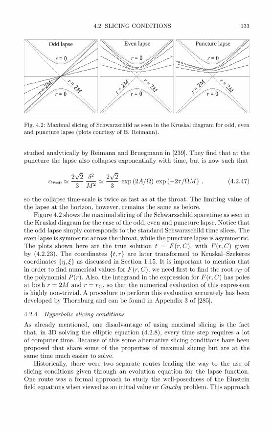
4.2 SLICING CONDITIONS 133
r = 0
r = 0
r = 2M
r = 2M
Odd lapse
r = 0
r = 0
Even lapse
r = 2M
r = 2M
r = 0
r = 0r = 2M
r = 2MPuncture lapse
Fig. 4.2: Maximal slicing of Schwarzschild as seen in the Kruskal diagram for odd, evenand puncture lapse (plots courtesy of B. Reimann).
studied analytically by Reimann and Bruegmann in [239]. They find that at thepuncture the lapse also collapses exponentially with time, but is now such that
αr=0 2√
23
δ2
M2 2
√2
3exp (2A/Ω) exp (−2τ/ΩM) , (4.2.47)
so the collapse time-scale is twice as fast as at the throat. The limiting value ofthe lapse at the horizon, however, remains the same as before.
Figure 4.2 shows the maximal slicing of the Schwarzschild spacetime as seen inthe Kruskal diagram for the case of the odd, even and puncture lapse. Notice thatthe odd lapse simply corresponds to the standard Schwarzschild time slices. Theeven lapse is symmetric across the throat, while the puncture lapse is asymmetric.The plots shown here are the true solution t = F (r, C), with F (r, C) givenby (4.2.23). The coordinates t, r are later transformed to Kruskal–Szekerescoordinates η, ξ as discussed in Section 1.15. It is important to mention thatin order to find numerical values for F (r, C), we need first to find the root rC ofthe polynomial P (r). Also, the integrand in the expression for F (r, C) has polesat both r = 2M and r = rC , so that the numerical evaluation of this expressionis highly non-trivial. A procedure to perform this evaluation accurately has beendeveloped by Thornburg and can be found in Appendix 3 of [285].
4.2.4 Hyperbolic slicing conditions
As already mentioned, one disadvantage of using maximal slicing is the factthat, in 3D solving the elliptic equation (4.2.8), every time step requires a lotof computer time. Because of this some alternative slicing conditions have beenproposed that share some of the properties of maximal slicing but are at thesame time much easier to solve.
Historically, there were two separate routes leading the way to the use ofslicing conditions given through an evolution equation for the lapse function.One route was a formal approach to study the well-posedness of the Einsteinfield equations when viewed as an initial value or Cauchy problem. This approach

134 GAUGE CONDITIONS
used the so-called harmonic coordinates, which are defined by asking for the waveoperator acting on the coordinate functions xα to vanish:
xα = gµν ∇µ∇ν xα = 0 . (4.2.48)
Harmonic coordinate conditions have the important property of allowing theEinstein field equations to be written as a series of wave equations (with non-linear source terms) for the metric coefficients gµν . Because of this, these condi-tions have been used in many analytical studies of the properties of the Einsteinequations, and in particular were used by Choquet-Bruhat to prove the firsttheorems on the existence and uniqueness of solutions to these equations [84](we will come back to the issue of the well-posedness of the Einstein evolutionequations in Chapter 5).
Expanding the harmonic coordinate condition (4.2.48) in adapted coordinateswe find
Γα := gµνΓαµν = 0 , (4.2.49)
where Γαµν are the Christoffel symbols associated with the 4-metric gµν . Concen-
trating on the condition for the time coordinate x0 = t, and using the expressionsfor the 4-Christoffel symbols in 3+1 language found in Appendix B, the aboveequation can be shown to reduce to
d
dtα ≡
(∂t − £β
)α = −α2K . (4.2.50)
This is known as the harmonic slicing condition. Notice that, through the ADMequations, this condition implies that
d
dtα = 0 , (4.2.51)
with α := α/√
γ the densitized lapse introduced in Chapter 2. This implies that,in the case of zero shift, harmonic slicing can also be written in integrated form asα = h(xi)
√γ, with h(xi) an arbitrary (but positive) time independent function.
It is very important to stress the fact that the integrated relation holds onlywhen moving along the normal direction to the hypersurfaces, and not whenmoving along the time lines which will differ from the normal direction for anynon-zero shift vector. That is, harmonic slicing relates the lapse to the volumeelements associated with the Eulerian observers.
A second route to the use of evolution type slicing conditions started withthe first three-dimensional evolution codes in the early 1990s. Since solving themaximal slicing condition was very time consuming, some attempts were madeto use algebraic slicing conditions, starting from the integrated form of harmonicslicing α =
√γ. However, it was quickly realized that such a slicing condition
was not very useful for evolving black hole spacetimes as it approached the sin-gularity very rapidly (we will see below that harmonic slicing is only marginally
4.2 SLICING CONDITIONS 135
singularity avoiding). This led to the empirical search for better behaved alge-braic slicing conditions [25, 54], and in particular resulted in the discovery thata slicing condition of the form α = 1 + ln γ, the so-called 1+log slicing, was veryrobust in practice and mimicked the singularity avoiding properties of maximalslicing.
Both routes finally merged with the work on hyperbolic re-formulations ofthe 3+1 evolution equations of Bona and Masso in the early and mid 1990s [62,63, 64]. This resulted in the Bona–Masso family of slicing conditions [65], whichis a generalization of harmonic slicing for which the lapse is chosen to satisfy thefollowing evolution equation
d
dtα = −α2f(α)K , (4.2.52)
with f(α) a positive but otherwise arbitrary function of α (the reason why f(α)has to be positive will become clear below). Notice that the particular case f = 1reduces to harmonic slicing, while f = N/α, with N constant, corresponds (in thecase of zero shift) to α = h(xi) + ln γN/2, so that N = 2 reduces to the standard1+log slicing. The Bona–Masso version of 1+log slicing, i.e. equation (4.2.52)with f = 2/α, has been found in practice to be extremely robust and wellbehaved for spacetimes with strong gravitational fields [13, 15, 30], and in recentyears has supplanted maximal slicing in most three-dimensional evolution codesdealing with either black holes or neutron stars.
Let us go back to condition (4.2.52). Taking an extra time derivative we find
d2
dt2α = −α2f
[d
dtK − α(2f + αf ′)K2
], (4.2.53)
with f ′ := df/dα. Using now the evolution equation for K, equation (4.2.5), wefind that (in vacuum)
d2
dt2α − α2fD2α = −α3f
[KijK
ij − (2f + αf ′) K2]. (4.2.54)
The last equation shows that the lapse obeys a wave equation with a quadraticsource term in Kij . It is because of this that we say that the slicing condi-tion (4.2.52) is a hyperbolic slicing condition: It implies that the lapse evolveswith a hyperbolic equation. The wave speed associated with equation (4.2.54)along a specific direction xi can be easily seen to be
vg = α√
fγii . (4.2.55)
Notice that this gauge speed will only be real if f(α) ≥ 0, which explains whywe asked for f(α) to be positive. In fact, f(α) must be strictly positive becauseif it were zero we would not have a strongly hyperbolic system (see Chapter 5).

136 GAUGE CONDITIONS
To see how the gauge speed vg is related to the speed of light consider fora moment a null world-line. It is not difficult to find that such a world-line willhave a coordinate speed along the direction xi given by
vl = α√
γii , (4.2.56)
so the gauge speed (4.2.55) can be smaller or larger that the speed of light de-pending on the value of f . In the particular case of harmonic slicing we havef = 1, so the gauge speed coincides with the speed of light, but for the 1+logslicing with f = 2/α the gauge speed can easily become superluminal. Havinga gauge speed that is larger than the speed of light does not in fact lead to anycausality violations, as the superluminal speed is only related with the propaga-tion of the coordinate system, and the coordinate system can be chosen freely.Physical effects, of course, still propagate at the speed of light.
A variation of the Bona–Masso slicing condition has also been proposed thathas the property that for static spacetimes it guarantees that the lapse functionwill not evolve [10, 17, 302]. This condition can easily be obtained by asking forthe evolution of the lapse to be such that
∂tα =αf(α)γ1/2
∂tγ1/2 , (4.2.57)
which results in∂tα = −αf(α)
(αK − Diβ
i)
. (4.2.58)
The modified condition then substitutes the Lie derivative of the lapse withrespect to the shift with the divergence of the shift itself (essentially the Liederivative of γ). This has the consequence that it will not result in the samefoliation of spacetime for a different shift vector, i.e. the foliation of spacetimewe obtain will depend on the choice of shift. However, having a slicing condi-tion that is compatible with a static solution might have advantages in somecircumstances.
4.2.5 Singularity avoidance for hyperbolic slicingsAs mentioned in our discussion of maximal slicing, a very important propertyof slicing conditions is that of singularity avoidance. The singularity avoidingproperties of the Bona–Masso slicing condition have been studied in [3, 66].Following [66], we will start our discussion of this issue by defining a focusingsingularity as a place where the spatial volume elements γ1/2 vanish at a boundedrate. Let us assume that such a singularity occurs after a finite proper time τs
away from our initial time slice (as measured by the normal observers). We willfurther say that we have a singularity of order m if γ1/2 approaches zero as
γ1/2 ∼ (τs − τ)m , (4.2.59)
with m some constant power (we will see below that the expected order of afocusing singularity is in fact m = 1). Notice that we must have m > 0 for there
4.2 SLICING CONDITIONS 137
to be a singularity at all, and m ≥ 1 for the singularity to be approached at abounded rate. From now on we will therefore assume that m ≥ 1. In the followinganalysis we will also assume that the shift vector vanishes, so our statements willcorrespond to the relation between the lapse and the normal volume elements.
In order to study the behavior of the lapse as the singularity is approached,we will start from the fact that the Bona–Masso slicing condition (4.2.52) impliesthe following relation between α and γ1/2
d ln γ1/2 =dα
αf(α), (4.2.60)
from which we find
γ1/2 = F (xi) exp∫
dα
αf(α)
, (4.2.61)
with F (xi) a time independent function. Also, from the definition of the lapsewe see that the elapsed coordinate time at the formation of the singularity willbe
∆t =∫ τs
0
dτ
α. (4.2.62)
Let us now consider what happens to the lapse as the volume elements γ1/2
approach zero. One possibility would be for α to remain finite as γ1/2 vanishes,which would clearly mean that the coordinate time remains finite at the singular-ity, so the singularity would not be avoided. Equation (4.2.61), however, impliesthat if the lapse remains always finite it is impossible for the volume elementsto vanish (remember that f(α) is never allowed to be zero). We then concludethat this case can never arise: The Bona–Masso slicing condition (4.2.52) alwayscauses the lapse to collapse when the volume elements approach zero, for anyf(α) > 0.
Since the lapse can not remain finite at a focusing singularity, we are left withonly two other possibilities: Either the lapse becomes zero at the singularity, orit becomes zero before reaching the singularity. The last case implies that thetime slices will stop advancing a finite coordinate time before the singularityis reached. We call such behavior strong singularity avoidance. If, on the otherhand, the lapse becomes zero at the singularity we could still find that theintegrated coordinate time is finite or infinite, depending on the speed at whichα approaches zero. We will say that a slicing is marginally singularity avoidingif the singularity is reached after an infinite coordinate time (but do notice thatmarginal singularity avoidance implies that we will get arbitrarily close to thesingularity after a finite time).
To see under which conditions we can have strong or marginal singularityavoidance we must say something about the form of the function f(α) as weapproach the singularity. For this analysis we will assume that as α approacheszero the function f(α) behaves as a power law
f(α) = Aαn , (4.2.63)

138 GAUGE CONDITIONS
with both A > 0 and n constants. Such an assumption implies that∫dα
αf(α)=
1A
∫dα
αn+1=
ln α1/A n = 0 ,−1/(nAαn) n = 0 .
(4.2.64)
Consider first the case n = 0. Equation (4.2.61) can now be integrated to find
γ1/2 ∼ exp(− 1
nAαn
). (4.2.65)
We then see that for n < 0 the volume elements remain finite as the lapseapproaches zero, in other words for this case we have strong singularity avoid-ance. Notice that 1+log family of slicing conditions f(α) = N/α corresponds ton = −1, which implies that it is singularity avoiding in a strong sense, explain-ing why it has been found to mimic maximal slicing in practice. If, on the otherhand, n > 0 then both the lapse and the volume elements go to zero at the sametime so we can at most have marginal singularity avoidance.
Let us now go back now to the case n = 0. Using again (4.2.61) we find that
γ1/2 ∼ α1/A ⇒ α ∼ γA/2 .
It is then clear that in this case α and γ1/2 also vanish at the same time.We then find that n < 0 guarantees strong singularity avoidance, while for
n ≥ 0 we can have at most marginal singularity avoidance. In order to see if inthis last case we reach the singularity in an infinite or a finite coordinate time weneed to study the behavior of α as a function of proper time τ as we approachthe singularity. Starting from equation (4.2.62) for the elapsed coordinate timewe find
∆t =∫ τs
0
dτ
α=∫ 0
α0
dτ/dα
αdα , (4.2.66)
with α0 the initial lapse. Equation (4.2.66) implies that if dτ/dα remains differentfrom zero as the lapse collapses then ∆t will diverge and we will have marginalsingularity avoidance. On the other hand, if dτ/dα vanishes at the singularity asαp with p > 0 (or faster), then the integral will converge and the singularity willbe reached in a finite coordinate time, i.e. the singularity will not be avoided.To find the behavior of dτ/dα as we approach the singularity, we notice thatequation (4.2.59) implies
d ln γ1/2
dτ= − m
(τs − τ). (4.2.67)
Using now equation (4.2.60) we find
dα/dτ
αf(α)= − m
(τs − τ), (4.2.68)

4.2 SLICING CONDITIONS 139
which can be integrated to give
τ = τs − exp(
1m
∫dα
αf(α)
). (4.2.69)
Substituting now f(α) = Aαn we obtain
τ =
τs − α1/mA n = 0 ,τs − exp [−1/(nmAαn)] n > 0 .
(4.2.70)
Consider first the case n > 0. The derivative of τ with respect to α thenbecomes
dτ
dα= − 1
mAαn+1exp
(− 1
nmAαn
), (4.2.71)
from which it is easy to see that as α approaches zero dτ/dα also approacheszero faster than any power. This means that the singularity is reached in a finitecoordinate time and the singularity is not avoided.
For n = 0 we have, on the other hand,
dτ
dα= − 1
mAα(1/mA−1) . (4.2.72)
The behavior of dτ/dα as the singularity is approached therefore depends on thesign of (mA− 1). We find that for mA < 1 the derivative dτ/dα goes to zero asa positive power of α and the singularity is reached in a finite coordinate time,while in case mA ≥ 1 the singularity is reached in an infinite coordinate timeand we have marginal singularity avoidance.
The final result is that, if f(α) behaves as f = Aαn for small α and we havea focusing singularity of order m, then for n < 0 we have strong singularityavoidance, and for n = 0 and mA ≥ 1 we have marginal singularity avoidance.In the cases n > 0, and n = 0 with mA < 1, the singularity is not avoided eventhough the lapse collapses to zero, i.e. the collapse of the lapse does not alwaysimply singularity avoidance.
We still have not addressed the issue of what value of m should be expected,that is, how fast do the volume elements collapse to zero at the singularity. It isin fact not difficult to give an estimate of this. First, notice that from the ADMequations the volume elements behave as
∂t ln γ1/2 = −αK , (4.2.73)
so along the normal lines we have (dτ = αdt)
d
dτln γ1/2 = −K . (4.2.74)
Consider now the evolution equation for K (4.2.5). Using the Hamiltonian con-straint we find

140 GAUGE CONDITIONS
∂tK − βi∂iK = α[R + K2 + 4π (S − 3ρ)
]. (4.2.75)
Now, according to the well known BKL conjecture (Belinskii, Khalatnikov andLifshitz [53]), in the approach to a singularity the velocity terms can be expectedto dominate (the solution is velocity term dominated or VTD), and both the Ricciscalar and the matter terms can be ignored compared to the quadratic term K2,so that along the normal lines we have
d
dτK ∼ K2 ⇒ K ∼ 1
τs − τ. (4.2.76)
Substituting this back into the evolution equation for γ1/2 we finally find
γ1/2 ∼ τs − τ . (4.2.77)
The expected order of the singularity is therefore m = 1. This means that forn = 1 we will have marginal singularity avoidance if A ≥ 1. In other words, thecase f = 1 corresponding to harmonic slicing marks the limit of the region withmarginal singularity avoidance.
There is one final important point to consider in the strongly singularityavoiding case n < 0. From the form of the slicing condition (4.2.52) we see thatif n ≤ −2, then as the lapse approaches zero we can not guarantee that ∂tα willalso approach zero. In fact, ∂tα could remain finite or even become arbitrarilynegative; the slices will therefore not only avoid the singularity, but will in factmove back away from it as the lapse function becomes negative. This type ofbehavior is not desirable as the time slices could easily stop being spacelike.If we want to guarantee that we have strong singularity avoidance without thelapse becoming negative we must therefore choose f(α) such that as α approacheszero n remains in the region −2 < n < 0. Since the 1+log family correspondsto n = −1 it is just in the middle of this region, making it a very good choiceindeed.
4.3 Shift conditions
Considerably less is know about shift conditions than about slicing conditions.The main reason is that simply taking the shift equal to zero works well in manycases. Still, there are indeed many proposals for how to choose the shift vector,and it is known that in some cases taking a zero shift vector is a very poor choice.In particular, evolving black hole spacetimes with a vanishing shift vector causesthe black hole horizon to grow rapidly in coordinate space (since the Eulerianobservers keep falling in), which means that eventually all the computationaldomain will be inside the black hole. This implies that for long-term evolutionsof black hole spacetimes it is crucial to have an outward pointing shift vectorthat will prevent the time lines from falling into the black hole. Also, in the pastfew years it has been realized that for systems with angular momentum (rotatingneutron stars or black holes), the dragging of inertial frames can be so severe
4.3 SHIFT CONDITIONS 141
that a non-zero rotational shift vector is absolutely essential in order to avoidhaving large shears developing in the spatial metric that will rapidly cause thesimulation to crash. This type of situation also occurs in the case of orbitingcompact objects, and it is because of this that the study of shift conditions hasbecome a topic of great relevance in the past few years.
Below I will discuss both the classic elliptic shift conditions and the recentlyproposed hyperbolic-type conditions that have been very successful in the contextof simulation of orbiting compact objects.
4.3.1 Elliptic shift conditions
The classic elliptic shift conditions where originally proposed by Smarr and Yorkin their work on the so-called radiation gauge in the late 1970s [272, 273]. Con-sider a congruence of timelike curves with unit tangent vector Zµ. The projectionoperator normal to Zµ is given by
Pµν = gµν + ZµZν . (4.3.1)
In terms of Pµν , the twist ωµν , strain θµν and acceleration ζµ of the congruenceare defined as
ωµν := Pαµ P β
ν ∇[αZβ] , (4.3.2)
θµν := Pαµ P β
ν ∇(αZβ) , (4.3.3)ζµ := Zν∇νZµ . (4.3.4)
The strain tensor θµν can be further decomposed into its trace θ = ∇µZµ, alsoknow as the expansion, and its free part σµν = θµν − (θ/3)Pµν , known as theshear. In terms of the quantities defined above, the covariant derivative of Zµ
can be expressed as∇µZν = ωµν + θµν − ζµZν . (4.3.5)
Assume now that our congruence corresponds to the world-lines of the Eule-rian observers. We then have Zµ = nµ, with nµ the normal vector to the spatialhypersurfaces. This immediately implies that ωµν = 0, since the congruence ishypersurface orthogonal. We also find ζµ = aµ, with aµ the acceleration of theEulerian observers, and θµν = −Kµν , with Kµν the extrinsic curvature.
The strain tensor θµν = −Kµν = 1/2£nγµν corresponds to motion along thenormal lines. In an analogous way, we can define a strain tensor along the timelies tµ in the following way
Θij :=12
£t γij = −αKij +12
£β γij , (4.3.6)
where we have only considered the spatial components, as the strain tensor isclearly purely spatial.
The strain tensor Θij just defined measures the change in both the size andform of the volume elements along the time lines. We can then try to use a shift

142 GAUGE CONDITIONS
vector to minimize some measure of the strain tensor in order to reduce as muchas possible the changes in the spatial metric itself. Smarr and York propose tominimize the non-negative square of the strain tensor ΘijΘij in a global senseover the spatial hypersurface. If we integrate ΘijΘij over the slice, variation withrespect to the shift vector βi can be shown to result in the equation
DjΘij = 0 ⇒ Dj (Diβj + Djβi) = 2Dj (αKij) , (4.3.7)
which can be rewritten as
D2βi + DiDjβj + Rijβ
j = 2Dj (αKij) , (4.3.8)
where the Ricci tensor appears when we commute covariant derivatives of theshift. This equation is known as the minimal strain shift condition and gives usthree elliptic equations that can be used to find the three components of theshift vector given appropriate boundary conditions.
The minimal strain condition minimizes a global measure of the change in thevolume elements associated with the time lines. However, as the change in thevolume is related to the trace of the extrinsic curvature K, it would seem betterto use the shift vector to minimize only the changes in the shape of the volumeelements, independently of their size. We then define the shear associated withthe time lines as the tracefree part of Θij :
Σij := Θij − 13γijΘ . (4.3.9)
Smarr and York call Σij the distortion tensor in order to distinguish it from theshear tensor σij associated with the normal lines. From the definition above wefind that the distortion tensor is given by
Σij = −αAij +12(Lβ)ij , (4.3.10)
where as before Aij = Kij − (γij/3) K is the tracefree part of the extrinsiccurvature, and (Lβ)ij is the conformal Killing form associated with the shift(see equation (3.2.7)):
(Lβ)ij := Diβj + Djβi − 23
γijDkβk . (4.3.11)
We can also rewrite the distortion tensor in a way that is perhaps more illustra-tive by noticing that (4.3.10) is equivalent to
Σij =12γ1/3£t γij , (4.3.12)
with γij = γ−1/3γij the conformal metric. The distortion tensor is thereforeessentially the velocity of the conformal metric.
4.3 SHIFT CONDITIONS 143
Minimizing now the integral of ΣijΣij over the spatial hypersurface withrespect to the shift yields the condition
DjΣij = 0 , (4.3.13)
which implies∆L βi = 2Dj
(αAij
), (4.3.14)
where the operator ∆L is defined as
∆L βi := Dj(Lβ)ij = D2βi + DjDiβj − 2
3DiDjβ
j
= D2βi +13
DiDjβj + Ri
jβj . (4.3.15)
Equation (4.3.14) is known as the minimal distortion shift condition, andagain gives us three elliptic equations for the three components of the shift.The minimal distortion condition is a very natural condition that will minimizechanges in the shape of volume elements during an evolution. It can also beshown that when the gravitational field is weak, it includes the TT gauge usedto study gravitational waves [273]. Still, the fact that it is given through threecoupled elliptic equations has meant that it has not been extensively used inthree-dimensional numerical simulations.
Notice that, in particular, the expression (4.3.12) for the distortion tensorimplies that the minimal distortion condition can also be written as
Dj
(∂tγ
ij)
= 0 . (4.3.16)
This is very closely related to a proposal of Dirac for finding an analog of theradiation gauge in general relativity [111, 273], for which he suggested using
∂j∂tγij = ∂t∂j γ
ij = 0 . (4.3.17)
Remarkably, this equation has been recently rediscovered in the context of theBSSNOK formulation of the 3+1 evolution equations. Notice that, from equa-tion (2.8.8), the conformal connection functions are given by Γi = −∂j γ
ij , so theabove gauge condition is equivalent to
∂tΓi = 0 , (4.3.18)
This shift condition, known as Gamma freezing, has been proposed as a naturalshift condition in the context of the BSSNOK formulation, as it freezes three ofthe independent degrees of freedom. To see the relationship between the minimaldistortion and Gamma freezing conditions we notice that the evolution equationfor the conformal connection functions (2.8.25) can be written in terms of Σij as
∂tΓi = 2∂j
(γ1/3Σij
). (4.3.19)
144 GAUGE CONDITIONS
More explicitly, we have
∂tΓi = 2e4φ[DjΣij − Γi
jkΣjk − 6Σij∂jφ]
. (4.3.20)
We then see that the minimal distortion condition DjΣij = 0, and theGamma freezing condition ∂tΓi = 0, are equivalent up to terms involving firstspatial derivatives of the conformal metric and the conformal factor. In particu-lar, all terms involving second derivatives of the shift are identical in both cases(but not so terms with first derivatives of the shift which appear in the distortiontensor itself). That the difference between both conditions involves Christoffelsymbols should not be surprising since the minimal distortion condition is covari-ant while the Gamma freezing condition is not.
Very recently there has been an important development in looking for morenatural shift conditions. Jantzen and York [168] have proposed a modified formof the minimal distortion shift vector that takes into account the new weightedconformal decomposition of symmetric tensors, and the role that the densitizedlapse plays in the ADM evolution equations (see Section 3.2.3). The proposalof Jantzen and York is to minimize the square of a lapse-corrected distortiontensor Σij/α (corresponding to the change of the conformal metric with respectto proper time), and use the full spacetime metric determinant as measure inthe integral (thus giving an extra factor α in the volume element). This newvariation results in the modified condition
Dj
(Aij/α
)= 0 ⇒ Dj
[(Lβ)ij
/2α− Aij]
= 0 , (4.3.21)
The difference between the original minimal distortion condition and themodified version is essentially the position of the factor α inside the divergence.However, the new version has a closer relationship to the initial data problem,in particular in terms of the conformal thin-sandwich approach of Section 3.3.To see this, we first rewrite the modified minimal distortion condition (4.3.21)in terms of conformal quantities using the transformations given in Chapter 3.We find that the new condition is equivalent to
Dj
[(Lβ)ij
/2α − Aij]
= 0 , (4.3.22)
Compare now this last equation with the expression for the conformal tracefreeextrinsic curvature in terms of the shift and the velocity of the conformal metric,equation (3.3.7). We see that if the shift vector satisfies the new minimal distor-tion condition, then the time derivative of the conformal metric uij will remaintransverse during the evolution, i.e. Dj u
ij = 0, so that only the transverse-traceless part of the conformal metric evolves (uij is traceless by construction).Thus the new shift condition reduces the evolution of the conformal metric toits “dynamical” part. This new version of minimal distortion is therefore more

4.3 SHIFT CONDITIONS 145
natural and is closer to the original motivation of finding a gauge in general rel-ativity that separates out the evolution of the physical degrees of freedom fromthe gauge degrees of freedom.
4.3.2 Evolution type shift conditionsJust as in the case of the lapse, solving the elliptic minimal distortion and Gammafreezing shift conditions is very computationally demanding in three dimensions(considerably more so than maximal slicing since there are three coupled equa-tions). Because of this, in the past few years, there has been a search for robustshift conditions that can be implemented as evolution equations for the shiftcomponents. One natural approach is based on the idea that in order to solveelliptic conditions numerically we usually replace such equations by parabolicequations in a fictitious time, and then evolve the parabolic equation until itssolution relaxes to the solution of the elliptic equation we are looking for. As-sume, for example, that we wish to solve Laplace’s equation with some givenboundary conditions of either Dirichlet or Newmann type:
D2φ = 0 . (4.3.23)
In practice we replace this equation with the heat equation
∂τφ = εD2φ , (4.3.24)
where τ is a fictitious time and ε > 0 is some constant that fixes the time-scale of relaxation. We can then start with arbitrary initial data and evolvethis equation until φ relaxes to a stationary solution that satisfies the givenboundary conditions. If we reach a stationary situation clearly we have ∂τψ = 0,so we have found the solution of the Laplace equation we wanted. In practice,direct relaxation methods to solve elliptic equations are very slow to convergeand are hardly ever used anymore. More powerful methods like multi-grid are thepreferred choice nowadays, but at their core they still use the relaxation idea. Themain problem has to do with the fact that numerical stability for an equation ofparabolic type like the heat equation requires that we take ∆τ ε(∆x)2, so thatas we refine the spatial grid the time step rapidly becomes prohibitively small.In principle, instead of using the heat equation we could substitute Laplace’sequation with the wave equation in fictitious time,
∂2τφ − v2D2φ = 0 , (4.3.25)
for which the restriction on the time step is much less severe and is given insteadby the CFL condition v∆τ ∆x, with v the characteristic speed of the system(see Chapter 9). However, this approach does not work well in practice sincethe wave equation with arbitrary boundary conditions will typically not relax aswaves keep getting reflected by the boundaries.39
39For some special boundary conditions, however, using the wave equation does work andconverges much faster than using the heat equation.
146 GAUGE CONDITIONS
An important development in the search for evolution-type gauge conditionswas the observation by Balakrishna et al. [46] that since in the case of the minimaldistortion condition we are actually solving for a gauge function, and the gaugeis arbitrary, it does not really matter too much if we have an exact solution tothe minimal distortion equation, as an approximate solution might already workextremely well in practice. We can therefore relax the elliptic equation in realtime instead of fictitious time. This led to the proposal of the so-called driverconditions, of which the first is the parabolic minimal distortion driver:
∂tβi = ε
[D2βi +
13
DiDjβj + Ri
jβj − 2Dj
(αAij
)], (4.3.26)
where the parameter ε > 0 is chosen small enough to guarantee numerical sta-bility in the range of resolutions considered, but large enough to allow the shiftto react to changes in the geometry.
We can now make a second observation. In practice we find that parabolicdrivers like the one introduced above usually do not allow the shift to respondrapidly enough to changes in the geometry unless ε is large, but in that case thenumerical stability of the whole evolution system rapidly becomes dominated bythe parabolic shift condition. One way to fix this is to use instead a hyperbolicdriver condition of the form
∂2t βi = α2ξ
[D2βi +
13
DiDjβj + Ri
jβj − 2Dj
(αAij
)], (4.3.27)
where now ξ > 0 is an arbitrary positive function of position and/or α thatcontrols the wave speed of the different shift components, and the explicit factorof α2 is there for later convenience when analyzing this wave speed (we will comeback to this issue below). At this point we might worry about the fact mentionedabove that relaxing via wave equations usually does not work since waves willreflect from the boundaries for generic boundary conditions. But again we noticethat we are solving for a gauge function, so we are also free to choose boundaryconditions any way we like. In particular, we can use outgoing wave boundaryconditions that allow the gauge waves to leave the computational domain withminimal reflections.
Driver conditions have recently become very important in the context ofthree-dimensional evolutions using the BSSNOK system of equations. As alreadymentioned, the minimal distortion condition is very closely related to the Gammafreezing condition (4.3.18). This has led to the suggestion of Alcubierre et al. ofusing a Gamma driver shift condition of the form [13]
∂2t βi = α2ξ ∂tΓi . (4.3.28)
In practice, a damping term is added to this condition to obtain
∂2t βi = α2ξ ∂tΓi − η ∂tβi , (4.3.29)
4.3 SHIFT CONDITIONS 147
where the parameter η > 0 is used to avoid strong oscillations in the shift (asimilar damping term can also be added to the minimal distortion driver).40
Both the hyperbolic minimal distortion driver and the hyperbolic Gammadriver provide us with shift conditions that will attempt to control the distor-tion of the volume elements with some time delay. In practice, the hyperbolicGamma driver condition has been found to be extremely robust and well be-haved in black hole simulations with puncture initial data, controlling both theslice stretching and the shear due to the rotation of the hole. The minimal dis-tortion hyperbolic driver condition has not been used extensively in practice, butwe could expect that it would be just as robust. In fact, on purely theoreticalgrounds the minimal distortion driver condition should probably be preferred asit results in a condition that is 3-covariant. The Gamma driver condition, onthe other hand, is clearly not 3-covariant implying that if we change our spatialcoordinates (say from Cartesian to spherical), we will obtain a different shift.
Before moving to a more general class of hyperbolic shift conditions, thereis an important point related to the characteristic speeds associated with thehyperbolic driver conditions that should be mentioned. A formal description ofhow to obtain such characteristic speeds will have to wait until Chapter 5, buthere we can anticipate some of the results. Notice that the hyperbolic minimaldistortion and Gamma driver conditions are in fact identical up to the principalpart (i.e. all terms with second derivatives are the same in both cases), so thattheir characteristic structure is the same. Consider first the asymptotically flatregion where the covariant derivatives can be substituted by partial derivatives. Itis easy to see that the characteristic speeds in that region along a fixed directionxi are
λl ±α√
4γiiξ/3 , λt ±α√
γiiξ , (4.3.30)
where here λl refers to the speed associated with the longitudinal shift compo-nent and λt to the speed associated with the transverse shift components, sothat longitudinal and transverse components propagate at different speeds. Innumerical simulations it is usual to take ξ = 3/4 (or ξ = αn3/4, with n someinteger), so that the longitudinal components propagate at the speed of lightasymptotically.41
There is yet another important point to make, related to the characteristicspeeds. A more formal analysis using the techniques described in Chapter 5shows that the characteristic cones associated with the shift modes for the driverconditions (4.3.27) and (4.3.29) have rather strange properties when comparedwith the characteristic cones associated with all other modes. For all other modes
40When using the Gamma driver shift, the specific value of the damping parameter η has animportant effect in achieving long-lasting evolutions of black hole spacetimes. Notice, however,that in contrast with ξ, the parameter η is not dimensionless, so that it must be scaled with thetotal mass of the spacetime M . The typical value used in black hole simulations is η ∼ 2/M .
41Recently it has been found that taking n = −2, which effectively makes the gauge speedsindependent of the lapse α, is a good choice in black hole simulations since it allows the shiftto evolve even in regions where the lapse has collapsed to zero.

148 GAUGE CONDITIONS
it turns out that the width of the characteristic cones is independent of the shift,and the shift’s only effect is to tilt the cones by −βi, which is precisely what wewould expect from the geometrical interpretation of the shift vector. In the caseof the driver conditions as given above we find, however, that the characteristiccones associated with the shift modes are only tilted by −βi/2, and also thattheir width depends on the magnitude of the shift. This unexpected behaviorcan be easily cured by changing the minimal distortion driver to
∂0βi = Bi , (4.3.31)
∂0Bi = α2ξ
[D2βi +
13
DiDjβj + Ri
jβj − 2Dj
(αAij
)], (4.3.32)
with ∂0 := ∂t−βi∂i. The Gamma driver condition is also changed in an analogousway to
∂0βi = Bi , (4.3.33)
∂0Bi = α2ξ ∂0Γi − ηBi . (4.3.34)
Apart from a trivial rewriting of the above conditions in first order in time form,all we have actually done is added an advection term to the time derivatives tofix the structure of the light cones. An advection term of this type was in factconsidered initially by the authors of [13] but later rejected (and never published)as it brings the shift condition to a form very similar to the simple equation∂tv − v ∂xv = 0, known as Burger’s equation, which is well know to result inthe formation of shocks. However, recent numerical simulations indicate that, atleast in the case of the Gamma driver condition, the advection terms do not giverise to shocks (the shift condition is coupled to all other dynamical equations, sothat this superficial resemblance to Burger’s equation is misleading). Moreover,in simulations of binary black hole systems with moving punctures [44] (seeChapter 6), it has been found that the inclusion of advection terms is importantin order to avoid having a perturbation in the constraints remaining at the initiallocation of the punctures.42
The driver conditions described above have been proposed as a way of findinga shift vector that is close to the solution of the corresponding elliptic equationsand at the same time is easy to solve for. As such these conditions, though cer-tainly robust in practice, are rather ad hoc. There is, however, a more naturalapproach to obtaining hyperbolic shift conditions similar to those used for thelapse. In Section 4.2.4 we introduced the idea of generalizing the condition fora harmonic time coordinate to obtain different slicing conditions. This led us
42Recently there has been both a formal analysis, and a series of numerical tests involvingmoving black holes, of variations in the way in which advection terms are be added to theGamma driver shift condition [156, 293] and their impact on the hyperbolicity of the systemand the accuracy of the numerical simulations.
4.3 SHIFT CONDITIONS 149
to the Bona–Masso family which has been found to be extremely successful inpractice. Recently, it has been suggested to use a similar approach to find hy-perbolic shift conditions as generalizations of the condition for harmonic spatialcoordinates [16].
Let us start from the harmonic condition for spatial coordinates
xi = 0 , (4.3.35)
which impliesΓi := gµνΓi
µν = 0 , (4.3.36)
with Γαµν the Christoffel symbols associated with the spacetime metric gµν . Using
the expressions found in Appendix B, we can easily show that in 3+1 languagethe above condition reduces to
∂tβi = βa∂aβi − α∂iα + α2 (3)Γi
+βi
α
(∂tα − βa∂aα + α2K
), (4.3.37)
where now (3)Γi is defined in terms of the three-dimensional Christoffel symbols(3)Γi
jk. This condition has in fact been known for a long time (see e.g. [140, 305]),though it is usually written down assuming that the lapse is also harmonic so thatthe term in parenthesis vanishes.43 Having the evolution equation for the shiftdepend on the time derivative of the lapse is clearly inconvenient if we want touse harmonic spatial coordinates with a different slicing condition, say maximalslicing. Remarkably, it turns out that if we rewrite the evolution equation for theshift in terms of a rescaled shift vector of the form σi = βi/α, then the spatialharmonic condition decouples completely from the evolution of the lapse so wecan work with an arbitrary slicing condition. We find
∂tσi = ασa∂aσi − ∂iα + α
(σiK + (3)Γi
). (4.3.38)
This can now be generalized in a natural way by considering instead thefollowing evolution equation for σi
∂tσl = ασm∂mσl − ∂lα + αh
(σlK + (3)Γl
), (4.3.39)
with h(α) > 0 an arbitrary function of the lapse [16]. The last condition isknown as the generalized harmonic shift condition, and is closely related to shiftconditions recently proposed by Lindblom and Scheel [190], and by Bona andPalenzuela [67]. It is not difficult to see that by choosing the free parametersin these references appropriately, we can in fact recover the above condition,but only provided we also take the lapse to evolve via the Bona–Masso slicingcondition (4.2.52) and take h(α) = f(α).
43Equation (4.3.37) fixes a sign error in [305], and includes a term missing in [140].

150 GAUGE CONDITIONS
There are several properties of the shift condition (4.3.39) that are importantto mention. First, in an analogous way to the Bona–Masso slicing condition, itleads to a characteristic speed associated with the shift modes of the form
λ = α(−σi ±
√hγii
)= −βi ± α
√hγii , (4.3.40)
so that we clearly must ask for h > 0. In fact, the function h plays exactly thesame role for the shift as the function f did in the case of the Bona–Masso slicingcondition. Notice also that the generalized harmonic shift condition (4.3.39) hasagain the Burger’s type structure ∂tv − v∂xv = 0, but a detailed analysis showsthat it does not lead to the formation of shocks (see [16] and also Chapter 5).
There is a final issue to discuss regarding the generalized harmonic shiftcondition (4.3.39). Notice that, just as was the case with the Gamma driver,this condition is not covariant with respect to changes in the spatial coordinates.That is, starting from exactly the same 3-geometry but with different spatialcoordinates we will get a different evolution of the shift vector. In particular,for curvilinear systems of coordinates we could find that even starting from aflat slice of Minkowski spacetime we would still have non-trivial shift evolutiondriven by the fact that the initial (3)Γi do not vanish. Worse still, in many casesit can happen that the (3)Γi of flat space are not only non-zero but are alsosingular, as is the case with spherical coordinates for which (3)Γr is of order 1/r.In response to this it has been suggested in [16] that the generalized harmonicshift condition should be interpreted as always being applied in a coordinatesystem that is topologically Cartesian.
Of course, we would still like to be able to express the condition in a generalcurvilinear coordinate system. Let us denote by xa the reference topologicallyCartesian coordinates, and by xi the general curvilinear coordinates. We findthat in the curvilinear coordinate system the shift condition should in fact bereplaced with
∂tσl = ασmDmσl − Dlα + αh σlK
+ α (hγmn − σmσn)∆lmn , (4.3.41)
where as before Di is the three-dimensional covariant derivative and where wehave defined
∆lmn := (3)Γl
mn − F lmn , (4.3.42)
withF i
jk := ∂axi ∂j∂kxa . (4.3.43)
The shift condition (4.3.41) is in fact 3-covariant, as we can readily verify thatthe ∆l
mn transform as the components of a 3-tensor. But the price we have paidis that we have chosen a privileged Cartesian coordinate system to be used as areference in order to define the F l
mn. A similar idea can also be used to obtain afully covariant version of the Gamma driver condition (4.3.28).
4.3 SHIFT CONDITIONS 151
In practice, we can use the fact that for flat space in Cartesian coordinatesthe Christoffel symbols vanish, which implies
F lmn = (3)Γl
mn
∣∣∣flat
, (4.3.44)
so that∆l
mn = (3)Γlmn − (3)Γl
mn
∣∣∣flat
. (4.3.45)
The covariant version of the generalized harmonic shift has been used success-fully in evolutions of spherically symmetric systems, but so far has not been triedin the full three-dimensional case where the hyperbolic Gamma driver conditionstill dominates.
4.3.3 Corotating coordinates
Consider a system of two orbiting compact objects (neutron stars or black holes).If the objects are sufficiently far away, the inspiral time-scale of the binary dueto emission of gravitational waves will be large compared to the orbital period.In such a case we can in fact use a shift vector to go to a corotating coordinateframe where the metric dynamics will be greatly reduced and numerical errorswill become smaller (in particular, numerical conservation of angular momentumwill improve in a corotating frame). Corotating coordinates have been used, forexample, in [114] for the case of binary neutron stars, and in [11, 80, 110] forthe case of binary black holes. Also, a shift vector corresponding to a corotatingframe is the expected result of the quasi-equilibrium approach to constructinginitial data for orbiting binaries (see Section 3.5.2), as only for such a shift canwe expect to have a quasi-stationary evolution.
Let us consider how we can implement a corotating reference frame. A firstapproach is simply to go to a frame that rotates with some fixed angular velocityΩ. Now let t, x, y, z be the non-rotating original coordinates and t, x, y, z bethe rotating coordinates. Assuming a rotation on the x-y plane, i.e Ω = Ω ez,the transformation of coordinates is given by
t = t , (4.3.46)z = z , (4.3.47)x = x cos (Ωt) − y sin (Ωt) , (4.3.48)y = x sin (Ωt) + y cos (Ωt) . (4.3.49)
This corresponds to the following gauge transformation
α = α , (4.3.50)
βi = βi +(Ω × ρ
)i
, (4.3.51)
with ρ := (x, y, 0). So in order to go to a corotating frame all we need to dois add a rigid rotation to the shift vector. Of course, we must know the correct

152 GAUGE CONDITIONS
value of the orbital angular velocity Ω, but this can usually be obtained (at leastapproximately) from the initial data.44
Notice that if we are using an elliptic shift condition like minimal distortion,the rigid rotation term will only fix the boundary condition, and the value ofthe shift in the interior will be given by the solution of the elliptic equation.If, on the contrary, we use an evolution equation for the shift, then the rigidrotation will fix the initial data for the shift everywhere. There is, however, animportant point that should be mentioned. Having an initial shift given by a purerigid rotation term assumes that we are working on a flat spacetime. In practicewe can expect this to work well in the asymptotically flat region far from thesources, but not in the inner regions where the spacetime can be far from flat.To see the type of problem we face let us consider for a moment maximal slicing(K = 0) and conformally flat initial data (γij = ψ4δij) for an orbiting binary,and an initial shift given by a rigid rotation as above. Now, the ADM evolutionequation for the volume elements implies that the conformal factor ψ evolves as
∂tψ = −ψ
6(αK − ∂iβ
i)
+ βi∂iψ . (4.3.52)
But in this case we have K = 0, and also for a rigid rotation it is easy to verifythat ∂iβ
i = 0. The last equation then reduces to
∂tψ − βi∂iψ = 0 . (4.3.53)
This is nothing more than the advection equation. We then find that ψ willkeep its original profile and will just advect with a speed given by −βi (atleast initially). The curious thing about this result is that naively we could haveexpected that some value of Ω would bring us to a corotating frame where ψessentially does not evolve, but we have instead found that given a rigid rotationwith any value of Ω, the conformal factor ψ will just start rotating the oppositeway, so we would have been better off having zero shift. Of course, this is onlyinitially, we would expect that if we have a good value of the angular velocityeverything would settle after some initial transient to the true corotating frame.
A extreme example of the situation just mentioned occurs for binary blackholes that use puncture type data. In that case the initial conformal factor be-haves as 1/r near the puncture, so that as long as K and ∂iβ
i remain regularwe will find that near the puncture the advection term βi∂iψ will dominate sothat again ψ will just advect with speed −βi. In other words, if the shift is notzero at the puncture then the puncture will move. Since the whole point of goingto a corotating frame is to have the black holes approximately stationary, wefind that the rigid rotation must be modified at the puncture position to ensure
44The effective potential method gives an approximate value of the angular velocity asΩ = ∂Eb/∂J , with Eb the effective potential energy and J the ADM angular momentum. Thequasi-equilibrium approach usually gives a much better value of Ω by asking for the Komarand ADM masses to be equal (see Chapter 3).

4.3 SHIFT CONDITIONS 153
that the shift becomes zero. The standard way to achieve this in practice is tomultiply the initial rigid rotation term with a negative power of ψ to guaranteethat the shift will vanish at the puncture [11, 80]:
βt=0 =1ψ3
Ω × ρ . (4.3.54)
The third power is chosen because this guarantees that the magnitude of theshift will become zero at the puncture in the non-conformal physical metric, andalso guarantees that the puncture will not evolve [13].
There is another important issue to consider when dealing with corotatingcoordinates. Notice that as we move away from the center of rotation, the mag-nitude of the rigid rotation shift vector increases as ρΩ. For a given value of Ωthere will then be a distance such that the shift will become superluminal – this isknown as the light-cylinder. We might then worry that outside the light-cylindercausality effects will cause problems with a numerical simulations. In fact, somesimple numerical methods do indeed become unstable when the light-cones tipbeyond the vertical, but this problem is in fact very easy to overcome. Methodsusing first-order in time evolution equations can be made to remain stable wellbeyond the light-cylinder by simply using one-sided differences for the advectionterms on the shift (i.e. terms of the form βi∂i). What we do have to worry aboutnumerically is the fact that, as the magnitude of the corotating shift vector in-creases with distance, the restrictions on numerical stability associated with theCFL condition become more severe and the time step must be taken smaller andsmaller.
There is, however, a serious issue related to causality for superluminal shiftvectors that has to do with the outer boundary conditions. If we are evolving ona cubical numerical grid and the boundary is located beyond the light-cylinder,then there will be regions of the boundary whose entire causal past is outsidethe computational domain (see Figure 4.3). We then have absolutely no physicalinformation that can be used to set up boundary conditions at those points.In real-life simulations, standard practice has been to just keep using the sameboundary conditions we would use for simulations with a small shift at the bound-ary and “hope for the best”, taking the pragmatic position that as long as theboundaries remain stable and are sufficiently far away we can live with unphys-ical boundary conditions. But it is well understood that the boundary issue is aserious problem for corotating grids. A much better solution would be to use acylindrical computational domain.
As already mentioned, although corotating frames seem attractive in somecircumstances, they have a series of disadvantages associated mainly with theboundary conditions applied at the edge of the computational domain. Anothermajor disadvantage is the fact that it is more difficult to extract gravitationalradiation from a corotating frame, plus this radiation will be seriously contami-nated by errors coming from the boundary conditions. Finally, recent advances

154 GAUGE CONDITIONS
Light-cylinder = 1
Fig. 4.3: The light-cylinder marks the boundary of the region where the shift becomessuperluminal (essentially ρΩ > 1); outside this region the light cones are tilted beyondthe vertical. The arrows at the boundaries indicate those points whose causal past iscompletely outside the computational domain so that there is no physical informationavailable to set up boundary conditions.
in gauge conditions and formulations of the evolution equations, and in partic-ular the development of new techniques that permit the simulation of binaryblack hole spacetimes without the need of singularity excision by allowing thepunctures to move [44, 93] (see Chapter 6), have shown that the use of coro-tating coordinates is not necessary to achieve stable and accurate numericalevolutions of binary black hole systems. Because of all this the use of corotat-ing coordinates is rapidly becoming less common, though they are still used inthe particular case of numerical codes based on spectral methods and multiplecoordinate patches [191].

5
HYPERBOLIC REDUCTIONS OF THE FIELD EQUATIONS
5.1 Introduction
When discussing the ADM equations in Chapter 2 we encountered the fact thatthe 3+1 evolution equations are not unique, as we can add arbitrary multiplesof the constraints to obtain new systems of evolution equations that will havethe same physical solutions but will differ in their unphysical (i.e. constraintviolating) solutions and, more importantly, in their mathematical properties.The original ADM equations differ from the standard version used in numericalrelativity (due to York) by precisely the addition of a term proportional to theHamiltonian constraint to the evolution equation of Kij . Also, the BSSNOKsystem uses both the Hamiltonian constraint to modify the evolution equationfor the trace of the extrinsic curvature K, and the momentum constraints tomodify the evolution equations for the conformal connection functions Γi.
There are of course an infinite number of ways in which we can add multiplesof the constraints to the evolution equations. The key question is then: Whichof these possible systems of equations will be better behaved both mathemati-cally and numerically? Historically, attempts to write down different physically-equivalent forms of the evolution equations for general relativity have followedtwo different routes: an empirical route that started in the late 1980s and lookedfor systems of equations that were simply better-behaved numerically than ADM,and a mathematically formal route that looked for well-posed, particularly hy-perbolic, reformulations of the evolution equations and that can be traced backto the work of Choquet-Bruhat in the 1950s on the existence and uniqueness ofsolutions to the Einstein equations [84]. In recent years these two approaches havefinally merged, and the traditionally more pragmatic numerical community hasrealized that well-posedness of the underlying system of evolution equations isessential in order to obtain stable and robust numerical simulations. At the sametime, it has been empirically discovered that well-posedness in not enough, assome well-posed formulations have been found to be far more robust in practicethan others.
From the early 1990s a large number of alternative formulations of the 3+1evolution equations have been proposed. We have now reached a point wheremore formulations exist than there are numerical groups capable of testing them.Because of this, here we will limit ourselves to discussing a small number of for-mulations, chosen both because they are a representative sample of the differentapproaches used, and because they correspond to the formulations used by themajority of numerical evolution codes that exist today. The discussion of well-
155
156 HYPERBOLIC REDUCTIONS
posedness and hyperbolicity presented here is of necessity brief and touches onlyon the main ideas, a more formal discussion can be found in the book by Kreissand Lorenz [177] (see also the review paper of Reula [241]).
5.2 Well-posedness
Consider a system of partial differential equations of the form
∂tu = P (D)u , (5.2.1)
where u is some n-dimensional vector-valued function of time and space, andP (D) is an n × n matrix with components that depend smoothly on spatialderivative operators.45 The Cauchy or initial value problem for such a systemof equations corresponds to finding a solution u(t, x) starting from some knowninitial data u(t = 0, x).
A crucial property of a system of partial differential equations like the oneconsidered above is that of well-posedness, by which we understands that thesystem is such that its solutions depend continuously on the initial data, orin other words, that small changes in the initial data will correspond to smallchanges in the solution. More formally, a system of partial differential equationsis called well-posed if we can define a norm || · || such that
||u(t, x)|| ≤ keαt||u(0, x)|| , (5.2.2)
with k and α constants that are independent of the initial data. That is, thenorm of the solution can be bounded by the same exponential for all initial data.
Most systems of evolution equations we usually find in mathematical physicsturn out to be well-posed, which explains why there has been some complacencyin the numerical relativity community about this issue. However, it is in factnot difficult to find rather simple examples of evolution systems that are notwell-posed. We will consider three such examples here. The easiest example isthe inverse heat equation which can be expressed as
∂tu = −∂2xu . (5.2.3)
Assume now that as initial data we take a Fourier mode u(0, x) = eikx. In thatcase the solution to the last equation can be easily found to be
u(x, t) = ek2t+ikx . (5.2.4)
We then see that the solution grows exponentially with time, with an exponentthat depends on the frequency of the initial Fourier mode k. It is clear that by
45One should not confuse the vectors we are considering here with vectors in the senseof differential geometry. A vector here only represents an ordered collection of independentvariables.

5.2 WELL-POSEDNESS 157
increasing k we can increase the rate of growth arbitrarily, so the general solutioncan not be bounded by an exponential that is independent of the initial data.This also shows that given any arbitrary initial data, we can always add to ita small perturbation of the form εeikx, with ε 1 and k 1, such that aftera finite time the solution can be very different, so there is no continuity of thesolutions with respect to the initial data.
A second example is the two-dimensional Laplace equation where one of thetwo dimensions is taken as representing “time”:
∂2t φ = −∂2xφ . (5.2.5)
This equation can be trivially written in first order form by defining u1 := ∂tφand u2 := ∂xφ. We find
∂tu1 = −∂xu2 , (5.2.6)∂tu2 = +∂xu1 , (5.2.7)
where the second equation simply states that partial derivatives of φ commute.Again, consider a Fourier mode as initial data. The solution is now found to be
φ = φ0ekt+ikx , u1 = kφ0e
kt+ikx , u2 = ikφ0ekt+ikx . (5.2.8)
We again see that the solution grows exponentially with a rate that dependson the frequency of the initial data k, so it can not be bounded in a way thatis independent of the initial data. This shows that the Laplace equation is ill-posed when seen as a Cauchy problem, and incidentally explains why numericalalgorithms that attempt to solve the Laplace equation by giving data on oneboundary and then “evolving” to the opposite boundary are bound to fail (nu-merical errors will explode exponentially as we march ahead).
The two examples above are rather artificial, as the inverse heat equationis unphysical and the Laplace equation is not really an evolution equation. Ourthird example of an ill-posed system is more closely related to the problem ofthe 3+1 evolution equations. Consider the simple system
∂tu1 = ∂xu1 + ∂xu2 , (5.2.9)∂tu2 = ∂xu2 . (5.2.10)
This system can be rewritten in matrix notation as
∂tu = M∂xu , (5.2.11)
with u = (u1, u2) and M the matrix
M =(
1 10 1
). (5.2.12)

158 HYPERBOLIC REDUCTIONS
Again, consider the evolution of a single Fourier mode. The solution of the systemof equations can then be easily shown to be
u1 = (ikAt + B) eik(t+x) , u2 = Aeik(t+x) , (5.2.13)
with A and B constants. Notice that u2 is oscillatory in time, so it is clearlybounded. However, u1 has both an oscillatory part and a linear growth in timewith a coefficient that depends on the initial data. Again, it is impossible tobound the growth in u1 with an exponential that is independent of the initialdata, as for any time t we can always choose k large enough to surpass any suchbound. The system is therefore ill-posed.
Systems of this last type in fact often appear in reformulations of the 3+1evolution equations (particularly in the ADM formulation). The problem can betraced back to the form of the matrix M above. Such a matrix is called a Jordanblock (of order 2 in this case), and has two identical real eigenvalues but can notbe diagonalized.
In the following Section we will consider a special type of system of partialdifferential equations called hyperbolic that can be shown to be well-posed undervery general conditions.
5.3 The concept of hyperbolicity
Consider a first order system of evolution equations of the form
∂tu + M i∂iu = s(u) , (5.3.1)
where M i are n × n matrices, with the index i running over the spatial dimen-sions, and s(u) is a source vector that may depend on the u’s but not on theirderivatives. In fact, if the source term is linear in the u’s we can show thatthe full system will be well-posed provided that the system without sources iswell-posed. We will therefore ignore the source term from now on. Also, we willassume for the moment that the coefficients of the matrices M i are constant.
There are several different ways of introducing the concept of hyperbolic-ity of a system of first order equations like (5.3.1).46 Intuitively, the conceptof hyperbolicity is associated with systems of evolution equations that behaveas generalizations of the simple wave equation. Such systems are, first of all,well-posed, but they also should have the property of having a finite speed ofpropagation of signals, or in other words, they should have a finite past domainof dependence.
We will start by defining the notion of hyperbolicity based on the properties ofthe matrices M i, also called the characteristic matrices. Consider an arbitraryunit vector ni, and construct the matrix P (ni) := M ini, also known as the
46One can in fact also define hyperbolicity for systems of second order equations (see forexample [154, 155, 212]), but here we will limit ourselves to first order systems as we canalways write the 3+1 evolution equations in this form.

5.3 THE CONCEPT OF HYPERBOLICITY 159
principal symbol of the system of equations (one often finds that P is multipliedwith the imaginary unit i, but here we will assume that the coefficients of theM i are real so we will not need to do this). We then say that the system (5.3.1)is strongly hyperbolic if the principal symbol has real eigenvalues and a completeset of eigenvectors for all ni. If, on the other hand, P has real eigenvalues for allni but does not have a complete set of eigenvectors then the system is said tobe only weakly hyperbolic (an example of a weakly hyperbolic system is preciselythe Jordan block considered in the previous Section). For a strongly hyperbolicsystem we can always find a positive definite Hermitian (i.e. symmetric in thepurely real case) matrix H(ni) such that
HP − PT HT = HP − PT H = 0 , (5.3.2)
where the superindex T represents the transposed matrix. In other words, thenew matrix HP is also symmetric, and H is called the symmetrizer. The sym-metrizer is in fact easy to find. By definition, if the system is strongly hyperbolicthe symbol P will have a complete set of eigenvectors ea such that (here theindex a runs over the dimensions of the space of solutions u)
Pea = λaea , (5.3.3)
with λa the corresponding eigenvalues. Define now R as the matrix of columneigenvectors. The matrix R can clearly be inverted since all the eigenvectors arelinearly independent. The symmetrizer is then given by
H = (R−1)T R−1 , (5.3.4)
which is clearly Hermitian and positive definite. To see that HP is indeed sym-metric notice first that
R−1PR = Λ , (5.3.5)
with Λ = diag(λa) (this is just a similarity transformation of P into the basis ofits own eigenvectors). We can then easily see that
HP = (R−1)T R−1P = (R−1)T ΛR−1 . (5.3.6)
But Λ is diagonal so that ΛT = Λ, which immediately implies that (R−1)T ΛR−1
is symmetric. Of course, since the eigenvectors ea are only defined up to an arbi-trary scale factor and are therefore not unique, the matrix R and the symmetrizerH are not unique either.
We furthermore say that the system of equations is symmetric hyperbolic ifall the M i are symmetric, or more generally if the symmetrizer H is independentof ni. Symmetric hyperbolic systems are therefore also strongly hyperbolic, butnot all strongly hyperbolic systems are symmetric. Notice also that in the caseof one spatial dimension any strongly hyperbolic system can be symmetrized,so the distinction between symmetric and strongly hyperbolic systems does not

160 HYPERBOLIC REDUCTIONS
arise. We can also define a strictly hyperbolic system as one for which the eigen-values of the principal symbol P are not only real but are also distinct for allni. Of course, this immediately implies that the symbol can be diagonalized, sostrictly hyperbolic systems are automatically strongly hyperbolic. This last con-cept, however, is of little use in physics where we often find that the eigenvaluesof P are degenerate, particularly in the case of many dimensions.
The importance of the symmetrizer H is related to the fact that we can useit to construct an inner product and norm for the solutions of the differentialequation in the following way
〈u, v〉 := u†Hv , (5.3.7)||u||2 := 〈u, u〉 = u†Hu , (5.3.8)
where u† is the adjunct of u, i.e. its complex-conjugate transpose (we will allowcomplex solutions in order to use Fourier modes in the analysis). In geometricterms the matrix H plays the role of the metric tensor in the space of solutions.The norm defined above is usually called an energy norm since in some simplecases it coincides with the physical energy.
We can now use the evolution equations to estimate the growth in the energynorm. Consider a Fourier mode of the form
u(x, t) = u(t)eikx·n . (5.3.9)
We will then have
∂t||u||2 = ∂t
(u†Hu
)= ∂t(u†)Hu + u†H∂t(u)
= ikuT PT Hu − ikuT HPu
= ikuT(PT H − HP
)u = 0 , (5.3.10)
where on the second line we have used the evolution equation (assuming s = 0).We then see that the energy norm remains constant in time. This shows thatstrongly and symmetric hyperbolic systems are well-posed. We can in fact showthat hyperbolicity and the existence of a conserved energy norm are equivalent,so instead of analyzing the principal symbol P we can look directly for theexistence of a conserved energy to show that a system is hyperbolic. Notice thatfor symmetric hyperbolic systems the energy norm will be independent of thevector ni, but for systems that are only strongly hyperbolic the norm will ingeneral depend on ni.
Now, for a strongly hyperbolic system we have by definition a complete setof eigenvectors and we can construct the matrix of eigenvectors R. We will usethis matrix to define the eigenfunctions wi (also called eigenfields) as
u = R w ⇒ w = R−1 u . (5.3.11)
Notice that, just as was the case with the eigenvectors, the eigenfields are onlydefined up to an arbitrary scale factor. Consider now the case of a single spatialdimension x. By multiplying equation (5.3.1) with R−1 on the left we find that

5.3 THE CONCEPT OF HYPERBOLICITY 161
∂tw + Λ ∂xw = 0 , (5.3.12)
so that the evolution equations for the eigenfields decouple. We then have a set ofindependent advection equations, each with a speed of propagation given by thecorresponding eigenvalue λa. This is the mathematical expression of the notionthat associates a hyperbolic system with having independent “wave fronts” prop-agating at (possibly different) finite speeds. Of course, in the multidimensionalcase the full system will generally not decouple even for symmetric hyperbolicsystems, as the eigenfunctions will depend on the vector ni.
We can in fact use the eigenfunctions also to study the hyperbolicity of a sys-tem; the idea here would be to construct a complete set of linearly independenteigenfunctions wa that evolve via simple advection equations starting from theoriginal variables ua. If this is possible then the system will be strongly hyper-bolic. For systems with a large number of variables this method is often simplerthan constructing the eigenvectors of the principal symbol directly, as findingeigenfunctions can often be done by inspection (this is in fact the method wewill use in the following Sections to study the hyperbolicity of the different 3+1evolution systems).
Up until now we have assumed that the characteristic matrices M i haveconstant coefficients, and also that the source term s(u) vanishes. In the moregeneral case when s(u) = 0 and M i = M i(t, x, u) we can still define hyperbol-icity in the same way by linearizing around a background solution u(t, x) andconsidering the local form of the matrices M i, and we can also show that strongand symmetric hyperbolicity implies well-posedness. The main difference is thatnow we can only show that solutions exist locally in time, as after a finite timesingularities in the solution may develop (e.g. shock waves in hydrodynamics,or spacetime singularities in relativity). Also, the energy norm does not remainconstant in time but rather grows at a rate that can be bounded independentlyof the initial data. A particularly important sub-case is that of quasi-linear sys-tems of equations where we have two different sets of variables u and v suchthat derivatives in both space and time of the u’s can always be expressed as(possibly non-linear) combinations of v’s, and the v’s evolve though equations ofthe form ∂tv + M i(u) ∂iv = s(u, v), with the matrices M i functions only of theu’s. In such a case we can bring the u’s freely in and out of derivatives in theevolution equations of the v without changing the principal part by replacing allderivatives of u’s in terms of v’s, and all the theory presented here can be ap-plied directly. As we will see later, the Einstein field equations have precisely thisproperty, with the u’s representing the metric coefficients (lapse, shift and spatialmetric) and the v’s representing both components of the extrinsic curvature andspatial derivatives of the metric.
First order systems of equations of type (5.3.1) are often written instead as
∂tu + ∂iFi(u) = s(u) , (5.3.13)
where F i are vector valued functions of the u’s (and possibly the spacetime

162 HYPERBOLIC REDUCTIONS
coordinates), but not of their derivatives. The vectors F i are called the fluxvectors, and it terms of them the characteristic matrices are simply given by
M iab :=
∂F ia
∂ub, (5.3.14)
that is, the matrices M i are simply the Jacobian matrices associated with thefluxes F i (notice that here i ∈ (1, 2, 3) runs over the spatial dimensions, while(a, b) ∈ (1, ..., n) run over the dimensions of the space of solutions). A system ofthe form (5.3.13) is called a balance law, since the change in u within a smallvolume element is given by a balance between the fluxes entering (or leaving) thevolume element and the sources. In the special case where the sources vanish,the system is called instead a conservation law. This is because in such a casewe can use the divergence theorem to show that if u has compact support thenthe integral of u over a volume outside such support is independent of time, i.e.it is conserved.
The simplest example of a strongly hyperbolic equation is of course the one-dimensional advection equation itself
∂tu + v ∂xu = 0 , (5.3.15)
with v a real constant. The solution of this equation simply propagates theinitial data with a speed v without changing its original profile. In other wordsif u(t = 0, x) = f(x), then u(t, x) = f(x − vt). Advection terms like this appearall the time in the 3+1 evolution equations, as the Lie derivative with respect tothe shift introduces terms of precisely the type βi∂i.
The next interesting example is the one-dimensional wave equation
∂2t φ − v2∇2φ = 0 , (5.3.16)
with v the wave speed. This equation can written in first order form by defining
Π := ∂tφ , (5.3.17)Ψi := v ∂iφ . (5.3.18)
The wave equation then turns into the system
∂tΠ − v∑
i
∂iΨi = 0 , (5.3.19)
∂tΨi − v ∂iΠ = 0 . (5.3.20)
Choose now a vector ni. The principal symbol is clearly
P (ni) = v
⎛⎜⎜⎝0 −nx −ny −nz
−nx 0 0 0−ny 0 0 0−nz 0 0 0
⎞⎟⎟⎠ . (5.3.21)

5.3 THE CONCEPT OF HYPERBOLICITY 163
Notice that the symbol is already symmetric, so the symmetrizer H is unityand the system is symmetric hyperbolic. Remembering now that the vector ni
is unitary (i.e. n2x + n2y + n2z = 1), we find that the eigenvalues of the principalsymbol are
λ1 = +v , λ2 = −v , λ3 = λ4 = 0 . (5.3.22)
So we have two degenerate eigenvalues and the system is not strictly hyperbolic.The matrix of column eigenvectors is given by
R(ni) =
⎛⎜⎜⎝1 1 0 0
−nx nx −nz −ny
−ny ny 0 nx
−nz nz nx 0
⎞⎟⎟⎠ , (5.3.23)
and its inverse is
R−1(ni) =
⎛⎜⎜⎝1/2 −nx/2 −ny/2 −nz/21/2 nx/2 ny/2 nz/20 −nz −nynz/nx (n2x + n2y)/nx
0 −ny (n2x + n2z)/nx −nynz/nx
⎞⎟⎟⎠ . (5.3.24)
The eigenfields then turn out to be (we have rescaled them for convenience)
w1 = Π −∑
i
niΨi , (5.3.25)
w2 = Π +∑
i
niΨi , (5.3.26)
w3 =∑
i
piΨi , (5.3.27)
w4 =∑
i
qiΨi , (5.3.28)
with p = (−nxnz,−nynz, n2x + n2y) and q = (−nynx, n2x + n2z,−nynz). Notice
that both pi and qi are orthogonal to ni. So we see that the longitudinal modes(parallel to ni) propagate at speeds ±v, and the transverse modes (orthogonalto ni) do not propagate. This example clearly shows that for symmetric hyper-bolic systems the eigenfields wa in general depend on the vector ni, even if thesymmetrizer does not.
Consider now the energy norm. Since the symmetrizer for the wave equationis unity (the principal symbol is already symmetric), our energy norm is simply
||u||2 = Π2 +∑
i
(Ψi)2 = (∂tφ)2 + v2
∑i
(∂iφ)2 , (5.3.29)
which in this case coincides with the physical energy density of the wave. Noticethat we should really understand this energy in an integrated sense:
164 HYPERBOLIC REDUCTIONS
E =∫
||u||2dV =∫ (
Π2 +∑
i
(Ψi)2
)dV . (5.3.30)
The change in time of the energy will then be
d
dtE =
d
dt
∫ (Π2 +
∑i
(Ψi)2
)dV = 2
∫ (Π ∂tΠ +
∑i
Ψi ∂tΨi
)dV
= 2v∑
i
∫(Π ∂iΨi + Ψi ∂iΠ) dV = 2v
∑i
∫∂i (ΠΨi) dV . (5.3.31)
The divergence theorem now implies that for initial data with compact supportdE/dt = 0.
As a final comment we should mention the fact there is one more equationthat we have left out of the above analysis, namely ∂tφ = Π. But this equationhas no fluxes and evolves only through a source term. If we included it in theanalysis we would simply have to add one new row and column to the matrixP with zeroes as entries. The result would be one more eigenfunction that doesnot propagate – namely φ itself. Since this does not add any new informationwe will generally leave out of the analysis the evolution equations of lower orderquantities such as φ.
5.4 Hyperbolicity of the ADM equations
We will now return to the 3+1 evolution equations and study under which con-ditions they are well-posed. In order to do this we will rewrite these equations asa system of the form (5.3.13), and study the structure of its characteristic matri-ces, i.e. its characteristic structure. There are many different ways in which wecan do this, the direct way would be to write down the principal symbols andfind its eigenvalues and eigenvectors. In some cases, however, it turns out thatwe can in fact discover the eigenfields by inspection. This is the method we willuse here and in the following Sections.
We will start by rewriting the standard ADM equations (2.3.11) and (2.5.5)described in Chapter 2
∂tγij − £βγij = −2αKij , (5.4.1)
∂tKij − £βKij = −DiDjα + α(Rij + KKij − 2KikKk
j
), (5.4.2)
where for simplicity we have assumed that we are in vacuum (the matter termscan in any case be considered as sources). This system is first order in time butsecond order in space, as the Ricci tensor Rij contains second derivatives of thespatial metric γij , and also there are second derivatives of the lapse function αin the evolution equation for Kij . In order to have a purely first order systemwe introduce the quantities
ai := ∂i ln α , dijk :=12
∂iγjk . (5.4.3)

5.4 HYPERBOLICITY OF THE ADM EQUATIONS 165
We will also assume that the shift vector βi is a known (i.e. a priori given)function of space and time. The lapse, on the other hand, will be considered adynamical quantity that evolves through an equation of the form
∂tα − βi∂iα = −α2Q , (5.4.4)
with the explicit form of the gauge source function Q to be fixed later.Since the characteristic structure is only related to the principal part, from
now on we will ignore all source terms, that is all terms that do not containderivatives of ai, dijk, and Kij . In terms of the dijk , the Ricci tensor can bewritten as
Rij −12γlm∂l∂mγij + γk(i∂j)Γk
−∂mdmij + 2 ∂(id
mmj) − ∂(idj)m
m , (5.4.5)
where here the symbol denotes “equal up to principal part”. There is in factan ordering ambiguity in the last expression, as the definition of dijk implies theconstraint
∂idjmn = ∂jdimn , (5.4.6)
so that we can write the Ricci tensor in different ways that are only equivalent ifthe constraint above is satisfied. However, here we will ignore this issue and usethe expression for the Ricci tensor given above (known as the De Donder–Fockdecomposition). We are now in a position to write down the evolution equationsfor ai, dijk and Kij :
∂0 ai −α ∂iQ , (5.4.7)∂0 dijk −α ∂iKjk , (5.4.8)∂0 Kij −α ∂kΛk
ij , (5.4.9)
where ∂0 := ∂t − βk∂k, and where we have defined (following [65])
Λkij := dk
ij + δk(i
(aj) + dj)m
m − 2dmmj)
). (5.4.10)
Notice that here we have another ordering ambiguity with the second derivativesof α, but this ambiguity can be resolved in a unique way by taking the explicitlysymmetric expression: ∂i∂jα = [∂i(αaj) + ∂j(αai)]/2.
As mentioned in the previous Section, for the characteristic analysis we willignore the evolution of the lower order quantities α and γij . We then have asystem of 27 equations to study corresponding to the three components of ai,the 18 independent components of dijk, and the six independent components ofKij .
To proceed with the characteristic analysis we will choose a specific directionx and ignore derivatives along the other directions; in effect we will only beanalyzing the matrix Mx. The reason why we can do this instead of analyzing

166 HYPERBOLIC REDUCTIONS
the full symbol P = niMi is that the tensor structure of the equations makes all
spatial directions have precisely the same structure, so it is enough to analyzejust one of them. The idea is then to find 27 independent eigenfunctions thatwill allow us to recover the 27 original quantities, where by eigenfunctions herewe mean linear combinations of the original quantities u = (ai, dijk, Kij) of theform wa =
∑b Cabub, that up to principal part evolve as ∂twa + λa∂xwa 0,
with λa the corresponding eigenspeeds. Notice that even if the coefficients Cab
should not depend on the u’s, they can in fact be functions of the lapse α andthe spatial metric γij (in order to avoid confusion we will use the Latin indicesat the beginning of the alphabet a, b, c, ... to identify the different fields, andthose starting from i, j, k, ... to denote tensor indices).
Then taking into account only derivatives along the x direction we immedi-ately see that there is a set of fields that propagate along the time lines withvelocity λ0 = −βx. These fields are
aq , dqij (q = x) . (5.4.11)
We have therefore already found 14 out of a possible 27 characteristic fields.Consider now the evolution equation for the Λx
pq, with p, q = x. Ignoringagain derivatives along directions different from x we find
∂0 Λxpq = ∂0 dx
pq −αγxx ∂xKpq , (5.4.12)
Comparing with (5.4.9) we see that we have found another set of characteristicfields that propagate along the light-cones with speeds47
λlight± = −βx ± α√
γxx . (5.4.13)
These eigenfields are √γxx Kpq ∓ Λx
pq . (5.4.14)
This gives us six new characteristic fields, so we now have a total of 20 out of27.
From this point on things become somewhat more complicated. Notice thatwe still need to find characteristic fields that will allow us to recover the sevenfields ax, dxxi, and Kxi. We start by writing down the evolution equation forΛx
xq:
∂0 Λxxq = ∂0 dx
xq +12
∂0 (aq + dqmm − 2dm
mq)
−αγxx ∂xKxq + α ∂xKxq
αγxp ∂xKpq . (5.4.15)
47Here we have used the observation that a pair of functions (u1, u2) that evolve throughequations of the form
∂tu1 = a ∂xu2 , ∂tu2 = b ∂xu1 ,
have the structure of the simple one-dimensional wave equation. The speeds of propagation forthis system are simply ±√
ab, and the corresponding eigenfields are w± = u1 ∓ (a/b)1/2u2.

5.4 HYPERBOLICITY OF THE ADM EQUATIONS 167
This equation presents us with a serious problem: It shows that while Kxq evolvesthrough derivatives of Λx
xq, the evolution of Λxxq is independent of Kxq and only
involves derivatives of Kpq. This subsystem can therefore not be diagonalized.Notice in particular that if the metric γij is diagonal then Λx
xq will remain con-stant up to principal part, which implies that Kxq will grow linearly unless Λx
xq
vanishes initially (of course, the presence of source terms makes things morecomplicated). This shows that the ADM system is not strongly hyperbolic; itis only weakly hyperbolic as we can in fact show that the eigenvalues of theprincipal symbol are all real.
We have then found that we can not recover the four quantities Kxq and Λxxq
(and hence dxxq) from characteristic fields. What about the quantities ax, dxxx,and Kxx? Even though we already know that the full system is not stronglyhyperbolic, there is still something very important to learn from these last threequantities. As it turns out, it is in fact easier to work with the traces K andΛx := γmnΛx
mn. The evolution equation for K clearly has the form
∂0 K −α ∂xΛx . (5.4.16)
The evolution equation for Λx, on the other hand, becomes
∂0 Λx = ∂0ax + 2 ∂0 (dxm
m − dmmx)
−αγxx ∂xQ − 2α (γxx ∂xK − ∂xKxx) . (5.4.17)
Notice first that this is the only equation that involves the gauge source functionQ, so that the explicit form of Q only affects the evolution of K and Λx (and ax
of course). Before discussing the form of Q let us for a moment recall the explicitform of the momentum constraints:
Dj
(Kij − γijK
)= 8πji , (5.4.18)
which up to principal part becomes
∂jKij − γij∂jK 0 . (5.4.19)
Considering now only derivatives along x we see that this implies, in particular,
∂xKxx γxx∂xK , (5.4.20)∂xKx
q 0 . (5.4.21)
This means that if the momentum constraints are satisfied identically the evo-lution equations for Λx
xq and Λx, equations (5.4.15) and (5.4.17), become
∂0 Λxxq −αγxx ∂xKxq (5.4.22)
∂0 Λx −αγxx ∂xQ (5.4.23)
This immediately solves our problem with the pair Kxq and Λxxq, as now they
behave exactly like Kpq and Λxpq, so this subsystem would also be strongly hy-
perbolic with the eigenfunctions√
γxx Kxq ∓ Λxxq propagating at the speed of
light.
168 HYPERBOLIC REDUCTIONS
On the other hand, for K and Λx we still need to say something about theform of Q. The simplest choice is to say that, just like the shift, the lapse is alsoan a priori known function of spacetime, in which case Q is just a source termand can be ignored. We can now clearly see, however, that this is a very bad ideaas we would then have Λx constant up to principal part and K evolving throughderivatives of Λx, which is precisely the same type of problem we had identifiedbefore. So having a prescribed lapse will result in a weakly hyperbolic systemeven if the momentum constraints are identically satisfied. Notice, however, thatif we were to take instead the densitized lapse α = α/
√γ as a prescribed function
of spacetime, then we would have(∂t − £β
)α =
α
2√
γ
(∂t − £β
)γ +
√γ(∂t − £β
)α
= −α2K +√
γ F (x, t) , (5.4.24)
with F (x, t) := (∂t−£β) α. This essentially means that Q = K (the second termcan be ignored as it contributes only to a source term). The equations for K andΛx would now become
∂0 K −α ∂xΛx , (5.4.25)∂0 Λx −αγxx ∂xK , (5.4.26)
so that we have another pair of modes propagating at the speed of light, namely√γxx K∓Λx. More generally, we can take a slicing condition of the Bona–Masso
family (4.2.52), which implies Q = f(α)K. The gauge eigenfields would then be√fγxx K ∓ Λx, and they would propagate with the gauge speeds
λgauge± = −βx ± α√
fγxx . (5.4.27)
These two gauge eigenfields will allow us to recover two of the three quantitiesax, dxxx, and Kxx. The last quantity can be recovered by noticing that
∂0 (ax − fdxmm) −α ∂x (Q − fK) = 0 , (5.4.28)
so that we have another independent eigenfield propagating along the time lines.We have then found that, provided that 1) the momentum constraints can
be guaranteed to be identically satisfied, and 2) either the densitized lapse α isassumed to be a known function of spacetime (but not the lapse itself), or weuse a slicing condition of the Bona–Masso family, then the ADM system wouldbe strongly hyperbolic.48
Taking a slicing condition of the Bona–Masso type is simple enough, butguaranteeing that the momentum constraints are identically satisfied is alto-gether a different matter. First, numerically the constraints will inevitably be
48In fact, we could also use maximal slicing since in that case K = 0 and the ai are obtainedthrough an elliptic equation. We would then have a coupled elliptic-hyperbolic system.
5.5 THE BONA–MASSO AND NOR FORMULATIONS 169
violated, and second, even at the continuum level strong hyperbolicity wouldonly be guaranteed for a very specific type of initial data, so the system wouldnot be well-posed as such. We are then forced to conclude that ADM is in factonly weakly hyperbolic. Still, we have learned two important lessons here: Thelapse itself can not be assumed to be a known function of spacetime, and themomentum constraints must play a crucial role.
As a final comment, notice that here we have only considered the standard(York) version of the ADM equations. The original ADM evolution equationsadd a multiple of the Hamiltonian constraint which makes the analysis somewhatmore difficult. Still, we will come back to the original ADM system in the nextSection.
5.5 The Bona–Masso and NOR formulations
In the last Section we showed that the standard ADM evolution system is onlyweakly hyperbolic and is therefore not well-posed. It is no wonder then that thefirst fully three-dimensional codes written in the early and mid 1990s based onthe ADM equations had serious stability problems (as we will see in Chapter 9,numerical stability can be seen essentially as a discrete version of well-posedness).Well-posed versions of the Einstein equations have in fact been known since the1950s and where used to prove the first theorems on the existence and unique-ness of solutions [84], but they were not based on a 3+1 decomposition andrequired the use of fully harmonic spacetime coordinates, so they were by andlarge ignored by the numerical community (but not completely, see e.g. [231] fora very recent and highly successful application of such techniques). Efforts tofind well-posed versions of the 3+1 evolution equations had to wait until the late1980s and early 1990s.
I will concentrate first on the Bona–Masso formulation, which is arguablythe simplest way to write down a strongly hyperbolic reformulation of the 3+1evolution equations [62, 63, 64, 65, 66].49 The Bona–Masso formulation starts bydefining the three auxiliary variables
Vi := dimm − dm
mi . (5.5.1)
In terms of the Vi, the Ricci tensor can be written up to principal part as
Rij −∂mdmij − ∂i
(Vj − 1
2djm
m
)− ∂j
(Vi − 1
2dim
m
). (5.5.2)
We then write the evolution equations for ai, dijk and Kij just as before as
49One often finds some confusion between the Bona–Masso family of slicing conditions de-scribed in Chapter 4 (and also used here), and the Bona–Masso formulation of the 3+1 evolutionequations. The Bona–Masso formulation uses their slicing condition, but the slicing conditionitself is in fact quite general and can be used with any form of the evolution equations.
170 HYPERBOLIC REDUCTIONS
∂0 ai −α ∂iQ , (5.5.3)∂0 dijk −α ∂iKjk , (5.5.4)∂0 Kij −α ∂kΛk
ij , (5.5.5)
where now
Λkij := dk
ij + δk(i
(aj) + 2Vj) − dj)m
m)
. (5.5.6)
Up to this point we have done nothing more than introduce a short-hand fora certain combination of d’s, but now we will take a big leap and consider theVi to be independent dynamical quantities in their own right and take theirdefinition (5.5.1) as a constraint. If the Vi are independent quantities we willneed an evolution equation for them, which can be obtained directly from theirdefinition. In order to write these evolution equations we first notice that
V i =12(dim
m − Γi)
, (5.5.7)
with Γi := γlmΓilm the contracted Christoffel symbols. We can show, after some
algebra, that
∂tΓi = £βΓi + γlm∂l∂mβi − Dl
[α(2Kil − γilK
)]+ 2αK lmΓi
lm , (5.5.8)
where the Lie derivative of Γi is to be understood as that of an ordinary vector.The fact that the Γi are not components of a true vector is what gives rise tothe term with the flat Laplacian of the shift. An interesting observation at thispoint is that we can rewrite the flat Laplacian of the shift as
γlm∂l∂mβi = D2βi − £βΓi − 2ΓilmDmβn + Ri
mβm , (5.5.9)
so that the evolution equation for Γi can be written in a more covariant-lookingway as
∂tΓi = D2βi+Rimβm−Dl
[α(2Kil − γilK
)]+2[αK lm − Dlβm
]Γi
lm . (5.5.10)
Using now the evolution equation for Γi we find that the Vi evolve up to principalpart as
∂0Vi α(∂jK
ji − ∂iK
). (5.5.11)
This is a very beautiful result, as it shows that the principal part of the evolutionequation for Vi is precisely the same as the principal part of the momentumconstraints.
Assume now that we add 2αM i to the evolution equation for Γi, whereM i := Dj
(Kij − γijK
)− 8πji = 0 are the momentum constraints. We are of
5.5 THE BONA–MASSO AND NOR FORMULATIONS 171
course perfectly free to do this as the physical solutions will remain the same.We would then have
∂tΓi = £βΓi + γlm∂l∂mβi − αγil∂lK
+ αal
(2Kil − γilK
)+ 2αK lmΓi
lm − 16πji , (5.5.12)
with ai = ∂i lnα as before. The evolution equation for the Vi up to principalpart now becomes
∂0Vi 0 , (5.5.13)
so that Vi evolves along the time lines.We can now repeat the analysis we did before for ADM, but now for the 30
independent quantities u = (ai, dijk, Kij , Vi). Considering as before only deriva-tives along the x direction we immediately see that there are now 17 fields thatpropagate along the time lines, namely
aq , dqij , Vi (q = x) . (5.5.14)
For Λxpq and Kpq with p, q = x, we find the same thing as in the ADM case, as
independently of the introduction of the Vi we still find that Λxpq = dx
pq, so thatagain we have the six eigenfields
√γxx Kpq ∓ Λx
pq , (5.5.15)
propagating along the light-cones.The difference with ADM is related to the remaining seven fields ax, dxxi,
and Kxi. For the evolution of Λxxq we now find
∂0 Λxxq = ∂0 dx
xq +12
∂0 (aq + 2Vq − dqmm)
−αγxx ∂xKxq , (5.5.16)
so that the four eigenfields√
γxx Kxq ∓ Λxxq , (5.5.17)
also propagate along the light-cones. Moreover, for the evolution of the traceΛx := γmnΛx
mn we now have
∂0 Λx = ∂0ax + 2 ∂0V
x
−αγxx ∂xQ . (5.5.18)
If we again take a slicing condition of the Bona–Masso type so that Q = f(α)K,we find the two gauge eigenfields√
fγxx K ∓ Λx , (5.5.19)
that propagate with the gauge speeds
λgauge± = −βx ± α√
fγxx . (5.5.20)
The last eigenfield is again ax − fdxmm which also propagates along the
time lines. In summary, we have 18 eigenfields propagating along the time lines,
172 HYPERBOLIC REDUCTIONS
namely aq, dqij , Vi, ax − fdxmm, 10 more eigenfields propagating along the light
cones, wliq± =
√γxx Kiq ∓ Λx
iq, and two gauge eigenfields wf± =
√fγxx K ∓ Λx.
The Bona–Masso formulation is therefore strongly hyperbolic as long as theevolution equation for the Vi is modified using the momentum constraints tomake its principal part vanish.
Instead of the Vi, we can choose to evolve the Γi as auxiliary quantitiesusing (5.5.12), and write the Ricci tensor Rij as
Rij −∂mdmij + ∂(iΓj) , (5.5.21)
which results in the Λkij being given by
Λkij = dk
ij + δk(i
(aj) − Γj)
). (5.5.22)
This is entirely equivalent since changing the Vi for the Γi only corresponds toa simple change of basis in the characteristic matrices, and does not alter theireigenvalues or eigenvectors.
The Bona–Masso formulation just presented can in fact be easily generalizedby introducing two parameters that corresponds to adding an arbitrary multipleof the momentum constraints to the evolution equation for the Γi (or equivalentlythe Vi), and a multiple of the Hamiltonian constraints to the evolution equationfor Kij . The resulting equations are known as the Nagy–Ortiz–Reula (NOR)formulation [212]. The NOR formulation modifies the evolution equations forKij in the following way
∂tKij − £βKij = −DiDjα + α(Rij + KKij − 2KikKk
j
)+ αηγijH , (5.5.23)
with H := R + K2 − KijKij − 16πρ = 0 the Hamiltonian constraint and η a
constant parameter. At the same time, the evolution equation for Γi is taken as
∂tΓi = £βΓi+γlm∂l∂mβi−Dl
[α(2Kil − γilK
)]+2αK lmΓi
lm+αξM i , (5.5.24)
where as before M i are the momentum constraints and ξ is also a constant pa-rameter. Notice that the particular case η = 0, ξ = 2 reduces to the Bona–Massoformulation.50 Also, the case η = ξ = 0 is essentially equivalent to the standardADM formulation (a la York), while ξ = 0 and η = −1/4 corresponds to theoriginal ADM formulation. The fact that the Γi are introduced as independentquantities has no effect if we take ξ = 0, since in that case their evolution equa-tions are not modified and the characteristic structure of the system is identicalto that of ADM with the addition of three extra eigenfields that propagate alongthe time lines, namely Γi − 2dm
mi + dimm.
50In fact, the Bona–Masso formulation also considered non-zero values of η, with the specialcases η = 0 and η = −1/4 called the “Ricci” and “Einstein” systems respectively.

5.5 THE BONA–MASSO AND NOR FORMULATIONS 173
The hyperbolicity analysis for the NOR system can be done in a numberof different ways. For example, Nagy, Ortiz, and Reula use a method based onpseudo-differential operators in order to analyze directly the second order systemwithout the need to introduce the first order quantities dijk [212]. For simplicity,however, here we will keep with our first order approach, but will not go into adetailed analysis since it proceeds in just the same way as before. If we againuse a slicing condition of the Bona–Masso type51, and consider only derivativesalong the x direction, we find that there are 18 fields that propagate along thetime lines with speed −βx; they are
aq, dqij , ax − fdxmm, Γi + (ξ − 2) dm
mi + (1 − ξ) dimm , (5.5.25)
with q = x. For the rest of the characteristic fields it turns out to be convenientto define the projected metric onto the two-dimensional surface of constant x ashij := γij − (sx)i(sx)j , with s x the normal vector to the surface:
(sx)i = δxi /
√γxx (sx)i = γxi/
√γxx . (5.5.26)
We can now use this projected metric to define the “surface-trace” of Kij as
K := hijKij = K − Kxx/γxx , (5.5.27)
with an analogous definition for Λx. Using this we find that the following char-acteristic fields
√γxx
(Kpq − hpq
2K
)∓(
Λxpq −
hpq
2Λx
), (p, q) = x , (5.5.28)
propagate along the light-cones with speeds
λlight± = −βx ± α√
γxx . (5.5.29)
Notice that these are only four independent eigenfields, since the combinationKpq − hpqK/2 is both symmetric and surface-traceless. This result is to be ex-pected, as these fields represent the transverse-traceless part associated with thegravitational waves. The four fields correspond to having two independent po-larizations that can travel in either the positive or negative x directions. Thetraces K and Λx also form an eigenfield pair given by
γxx [1 + 2η (2 − ξ)]1/2 K ∓ Λx , (5.5.30)
propagating with the speeds
λtrace± = −βx ± α γxx [1 + 2η (2 − ξ)]1/2 . (5.5.31)
Notice that for ξ = 2 these two fields also propagate at the speed of light.
51The original NOR system in fact does not use the Bona–Masso slicing condition, but rathertakes a general densitized lapse of the form Q = αγ−σ/2, with σ =constant, as a fixed functionof spacetime. The results, however, are entirely equivalent to the ones discussed here if we takeσ = f .

174 HYPERBOLIC REDUCTIONS
Another set of four eigenfields, corresponding to the longitudinal componentsof the extrinsic curvature, turns out to be given by√
γxx(ξ/2) Kxq ∓ Λxx
q , (5.5.32)
with a characteristic speed of
λlong± = −βx ± α√
γxx(ξ/2) . (5.5.33)
Again, for ξ = 2 these fields propagate along the light-cones.The last two eigenfields are again related to the gauge choice, and propagate
with the gauge speedsλgauge± = −βx ± α
√fγxx . (5.5.34)
These fields are √fγxx
(K + FK
)∓(Λx + F Λx
), (5.5.35)
with F := (1 + 3η)(2 − ξ)/[f − 1 − 2η(2 − ξ)].Collecting all these results we find that the NOR system is strongly hyperbolic
if the function f(α) and the parameters η and ξ fall into any of the three cases:
1. η = 0, ξ = 2 and f > 0.2. η = 0, ξ > 0, f > 0, and f = 1.3. η = 0, ξ > 0, f > 0, and η (2 − ξ) > −1/2.
We see that if we take η = 0 and ξ = 2, then the system is strongly hyperbolicfor any f > 0, but this we already knew as it corresponds to the Bona–Massosystem. More generally, if we take η = 0 and any ξ > 0, the system remainsstrongly hyperbolic as long as f > 0 and f = 1. This case, however, is probablynot very useful as it explicitly excludes harmonic slicing f = 1. More interestingis the last case that shows that we can take any f > 0 and any ξ > 0, providedthat η = 0 and η (2 − ξ) > −1/2. Notice that standard ADM corresponds toη = ξ = 0, so that it fails to be strongly hyperbolic since in all cases theparameter ξ must be strictly positive. The original ADM system, with η = −1/4and ξ = 0, is in fact worse as it would in principle fall into the third case but itfails to satisfy two of the necessary inequalities, since we now have both ξ = 0 andη (2 − ξ) = −1/2. By “worse” here we mean that there will be a smaller numberof independent eigenfunctions, but in any case both versions of the ADM systemare still weakly hyperbolic since they violate the inequalities only marginally andthe eigenspeeds are still real (satisfying the reversed inequalities would result insystems that are not even weakly hyperbolic as the eigenspeeds would becomecomplex). Taking ξ = 2, as in the Bona–Masso case, seems to be an optimalchoice as in that case all fields other than those related to the slicing conditionpropagate either along the time lines or with the speed of light. Also, in that casethe value of η plays no role in any of the eigenfields or eigenspeeds, so we arefree to choose an arbitrary value without affecting the characteristic structurein any way (using different values of η in this case might in fact improve the

5.6 HYPERBOLICITY OF BSSNOK 175
numerical stability as even though the characteristic structure in unaffected, thesource terms will certainly change, but this issue has not been studied in anydetail).
5.6 Hyperbolicity of BSSNOK
As already mentioned in Chapter 2, in the past few years the BSSNOK formu-lation has become the most widely used in three-dimensional numerical codesbased on the 3+1 decomposition.52 The reason for this is that this formulationhas been found to be very robust in practice in a large class of systems withstrong and dynamical gravitational fields, both with and without matter. In theoriginal paper of Baumgarte and Shapiro [50], the success of the new formulationwas attributed to the fact that it had a “more hyperbolic flavor”. This statementwas later put on somewhat ground by Alcubierre et al. in [6]. Finally, Sarbachet al. showed that the BSSNOK formulation is in fact strongly hyperbolic [249],so it should come as no surprise that it behaves better than ADM which, as wehave seen, is only weakly hyperbolic. Hyperbolicity, however, is clearly not theonly important property of this formulation, because BSSNOK has also beenfound empirically to out-perform other strongly hyperbolic formulations, suchas the Bona–Masso formulation presented in the previous Section. Since themain difference between these two formulations is the conformal decompositionof BSSNOK, such a decomposition clearly seems to be important, though at thispoint it is still not understood why this should be so.
The BSSNOK formulation takes as independent variables the conformal met-ric γij , the conformal factor φ, the trace of the extrinsic curvature K, the con-formally rescaled tracefree extrinsic curvature Aij , and the contracted conformalChristoffel symbols Γi := γmnΓi
mn, plus the lapse α and shift vector βi. In orderto study its characteristic structure we will again introduce the spatial derivativesof α, γij , and φ as independent quantities,
ai := ∂i ln α , dijk :=12
∂iγjk , Φi := ∂iφ , (5.6.1)
and assume the shift to be a given function of spacetime. For the hyperbolicityanalysis we now have to consider the 30 quantities u = (ai, Φi, dijk, K, Aij , Γi).Notice that these are in fact only 30 quantities and not 34, as Aij is tracelessby definition, and also γjkdijk = 0 as a consequence of the fact that γij hasunit determinant. The evolution equations guarantee that if these constraintsare satisfied initially they will remain satisfied during evolution (numerically,however, we finds that this does not hold exactly and the trace of Aij drifts, sothat the constraint trAij = 0 must be actively enforced during a simulation).
52At the time of writing this text, BSSNOK has become the dominant formulation usedin 3D numerical relativity, and is used in one way or another in practically all 3+1 basedcodes. The only real contenders to BSSNOK are hyperbolic formulations that evolve the fullfour-dimensional spacetime metric and are not directly based on the 3+1 formalism [191, 231].
176 HYPERBOLIC REDUCTIONS
Starting from the BSSNOK evolution equations of Section 2.8, we find thatup to principal part the evolution equations for our dynamical quantities become
∂0 ai −α ∂iQ , (5.6.2)
∂0 Φi −16
α ∂iK , (5.6.3)
∂0 dijk −α ∂iAjk , (5.6.4)∂0 K −αe−4φγmn∂man (5.6.5)
∂0 Aij −αe−4φ∂kΛkij , (5.6.6)
∂0 Γi α∂k
[(ξ − 2) Aik − 2
3ξγikK
], (5.6.7)
where we have now defined
Λkij :=
[dk
ij + δk(i
(aj) − Γj) + 2Φj)
)]TF
, (5.6.8)
and where we have allowed for an arbitrary multiple of the momentum constraintto be added to the evolution equation for Γi (standard BSSNOK corresponds tochoosing ξ = 2). In the following we will again assume that we are using a slicingcondition of the Bona–Masso family so that Q = fK.
For the hyperbolicity analysis we again consider only derivatives along thex direction. Again we immediately find that there are 18 fields that propagatealong the time lines with speed −βx:
aq , Φq , dqij , ax − 6fΦx , Γi + (ξ − 2) dmmi − 4ξ γikΦk , (5.6.9)
with q = x (again, these are only 18 fields since dqij is traceless). Now, the factthat in the BSSNOK formulation the trace of the extrinsic curvature K has beenpromoted to an independent variable and the Hamiltonian constraint has beenused to simplify its evolution equation, makes the gauge eigenfields very easy toidentify. The two gauge eigenfields are
e−2φ√
fγxxK ∓ ax , (5.6.10)
which propagate with the gauge speeds
λgauge± = −βx ± αe−2φ√
fγxx . (5.6.11)
There is another set of four eigenfields that again correspond to longitudinalcomponents and are be given by
e2φ√
γxx (ξ/2) Axq ∓ Λxx
q , (5.6.12)
with corresponding characteristic speeds
λlong± = −βx ± αe−2φ√
γxx (ξ/2) . (5.6.13)
These eigenfields in fact correspond to the fields (5.5.32) of the NOR formulationdiscussed in the previous Section. Notice that for standard BSSNOK we have

5.6 HYPERBOLICITY OF BSSNOK 177
ξ = 2, so that these eigenfields propagate along the light-cones. In any case, wesee that we must have ξ > 0 for the characteristic speeds to be real.
The transverse-traceless part is now represented by the eigenfields
e2φ√
γxx
(Apq +
γpq
2γxxAxx
)∓(
Λxpq +
γpq
2γxxΛxxx
), (5.6.14)
with p, q = x, which propagate with speeds
λlight± = −βx ± αe−2φ√
γxx , (5.6.15)
i.e. along the light-cones. There are in fact only four independent eigenfieldshere, because we can easily check that
Apq +γpq
2γxxAxx = e−4φ
(Kpq − hpq
2K
), (5.6.16)
with hij the metric tensor projected onto the surface of constant x introduced inthe previous Section and K = hijKij . These eigenfields are therefore symmetricand surface-traceless, so that they have only four independent components.
The final two characteristic fields represent the trace of the transverse com-ponents and are given by
e2φ√
γxx(2ξ − 1)/3(
Axx − 23γxxK
)∓(
Λxxx − 23γxx ax
), (5.6.17)
where ax := γxmam. These eigenfields propagate with the characteristic speeds
λtrace = −βx + αe−2φ√
γxx(2ξ − 1)/3 , (5.6.18)
which will only be real if
2ξ − 1 > 0 ⇒ ξ > 1/2 . (5.6.19)
We then conclude that the generalized BSSNOK system is strongly hyperboliconly for ξ > 1/2. The standard BSSNOK system corresponding to ξ = 2 is againan optimal choice, as in that case all eigenfields other than those associatedwith the gauge propagate either along the time lines or along the light-cones.It is important to observe that the BSSNOK system with no modification ofthe evolution equation for the Γi, i.e. ξ = 0, is not even weakly hyperbolic asthe eigenspeeds (5.6.18) become complex, so this choice would be far worse thanADM.
As a final observation it should be mentioned that Sarbach et al. [249] havealso shown that in some special cases the generalized BSSNOK system can bemade to be symmetric hyperbolic. In order to see this, we will attempt to write

178 HYPERBOLIC REDUCTIONS
down a conserved energy norm for this system that is independent of any partic-ular direction. By “conserved” what we really mean here is that up to principalpart its time derivative can be written as a full divergence, so that its integralin space vanishes for data of compact support.
The energy norm must be positive definite, and must include all the 30 inde-pendent fields we are considering. In order to construct this energy norm we willstart by noticing that the terms corresponding to fields that propagate along thetime lines are trivial. For example,
∂t (an − 6fΦn)2 2γmn (am − 6fΦm) ∂t (an − 6fΦn)= −2αγmn (am − 6fΦm) (f − f) ∂nK = 0 , (5.6.20)
where again we are only considering principal terms. Here and in what follows,the square of an object with indices will be understood as the norm calculatedusing the conformal metric, i.e. (Tn)2 ≡ γmnTmTn and so on. In a similar waywe also find that
∂t
(Γn + (ξ − 2)dm
mn − 4Φn
)2 0 . (5.6.21)
So we already have two terms in the energy norm. The gauge sector is also easilyfound, as we have
∂tK2 −2αKe−4φγmn∂man , (5.6.22)
∂t (an)2 −2αfγmnan∂mK , (5.6.23)
so that
∂t
[K2 +
e−4φ
f(an)2
] −2∂m (αγmnanK) , (5.6.24)
that is, we have a complete divergence.For the energy terms involving Amn and dkmn we notice that
∂t
(dkmn
)2 −2α dkmn∂kAmn , (5.6.25)
∂t
(Amn
)2 −2α e−4φAmn
[∂kdk
mn + ∂m
(an − Γn + 2Φn
)]. (5.6.26)
The time derivative of (Amn)2 involves terms other than the divergence of dkmn,so we need to study how these other terms evolve. Consider then
∂t
(an − Γn + 2Φn
)2 2γmn
(an − Γn + 2Φn
)∂t
(am − Γm + 2Φm
)(5.6.27)
−2α(an − Γn + 2Φn
) [(ξ − 2) ∂lA
lm −(
2ξ − 13
− f
)∂mK
]. (5.6.28)
The first term involves a divergence of Amn so that we can in principle use ittogether with the time derivative of (Amn)2 to form a total divergence, but the

5.7 THE KIDDER–SCHEEL–TEUKOLSKY FAMILY 179
second term involving the gradient of K spoils this. In order to build our totaldivergence we must then ask for
2ξ − 13
− f = 0 ⇒ ξ =1 + 3f
2. (5.6.29)
This means that if we want to have a symmetric hyperbolic system, the amount ofmomentum constraint added to the evolution equation for Γi must be determinedby the gauge source function f . Doing this we find that
∂t
[(Amn
)2+ e−4φ
(dkmn
)2+
e−4φ
ξ − 2
(an − Γn + 2Φn
)2](5.6.30)
−2αe−4φ
∂k
(Amndk
mn
)+ ∂k
[Akm
(an − Γn + 2Φn
)], (5.6.31)
so we have another total divergence. Collecting terms we obtain the followingfinal expression for the conserved energy norm
E = (an − 6fΦn)2 +(Γn + (ξ − 2)dm
mn − 4Φn
)2+ K2 +
e−4φ
f(an)2
+(Anm
)2+ e−4φ
(dkmn
)2+
e−4φ
ξ − 2
(an − Γn + 2Φn
)2. (5.6.32)
Notice that since the energy norm must be positive definite, we must also askfor ξ > 2, as otherwise the last term would be negative. In particular, standardBSSNOK with ξ = 2 is not symmetric hyperbolic. The restriction ξ > 2, togetherwith f = (2ξ − 1)/3, implies that we must also have f > 1 (i.e. the gaugespeed must be superluminal), so that for the BSSNOK family we cannot havea symmetric hyperbolic system with harmonic slicing. However, for the case of1+log slicing with f = 2/α, the above restriction implies α < 2 which willtypically always be satisfied (the lapse usually collapses below 1 in the presenceof a gravitational field – it does not grow), so that we could in principle use asymmetric hyperbolic version of BSSNOK with 1+log slicing.53
5.7 The Kidder–Scheel–Teukolsky family
As mentioned in the previous Sections, the Bona–Masso, NOR and BSSNOKformulations are closely related to each other and in particular follow the sameroute to obtain a strongly hyperbolic system. The main idea in those formula-tions is to introduce three new independent quantities related to contractionsof the Christoffel symbols associated with either the physical or the conformalmetric, and then to modify the evolution equations for these quantities using the
53Gundlach and Martın-Garcıa have in fact found a different conserved energy norm for BSS-NOK (i.e. a different symmetrizer) for which all characteristic speeds can remain causal, andthat, in particular, allows us to have a symmetric hyperbolic system with harmonic slicing [154].Such an energy norm, however, involves mixed terms of the form γnldm
mn(al − Γl + 2Φl), sothat showing that it is positive definite becomes considerably more difficult.
180 HYPERBOLIC REDUCTIONS
momentum constraints. These formulations also remain second order in space,though they can trivially be rewritten as fully first order formulations by intro-ducing the first derivatives of the spatial metric dijk as independent quantitiesand considering their definitions dijk := ∂iγjk/2 as new constraints (which iswhat we have done in order to study their hyperbolicity properties). An impor-tant point is that in these first order versions the evolution equations for the dijk
are obtained directly from their definition and are left unmodified. This has theconsequence that the derivative constraints remain trivially satisfied if they weresatisfied initially (even at the numerical level it is possible to arrange things sothat these constraints remain satisfied to the level of machine round-off error).
There is a different approach that can be used to obtain hyperbolic formula-tions of the 3+1 evolution equations based on the idea of going to a fully firstorder system and modifying directly the evolution equations for the dijk usingthe momentum constraints, but without introducing extra independent quanti-ties like the V i of Bona–Masso or the Γi of BSSNOK. This approach can betraced back to the work of Frittelli and Reula [135], and Anderson and York [21](the so-called Einstein–Christoffel formulation) from the mid and late 1990s. Themost general version of these type of formulations is known as the Kidder–Scheel–Teukolsky (KST) family and has twelve free parameters [172] (there have beensome further generalizations of this idea that have resulted in formulations witheven more free parameters, see e.g. [250]). Here, however, we will limit ourselvesto presenting a very simplified version of KST with only three free parametersthat nevertheless includes the main features of this formulation.
The KST system starts by introducing the derivatives of the spatial metricas independent quantities
dijk :=12
∂iγjk . (5.7.1)
The factor 1/2 above in fact does not appear in the original KST formulation,but here we introduce it in order to have a notation consistent with that of theprevious Sections.
For the Ricci tensor we use again (5.5.2), which we rewrite here for complete-ness
Rij −∂mdmij − ∂(i
(2Vj) − dj)m
m)
, (5.7.2)
with the Vi given byVi := dim
m − dmmi . (5.7.3)
Notice that these are the same quantities used in the Bona–Masso formulation,but here we will not promote them to independent variables and will insteadconsider them just a shorthand for the given combination of d’s. It is importantto mention the fact that in the standard KST formulation a parameter is addedto the above expression for the Ricci tensor Rij to allow for different ways toresolve the ordering ambiguity of the second derivatives of the metric. However,in order to simplify the system, here we have chosen the same specific orderingused in previous Sections.

5.7 THE KIDDER–SCHEEL–TEUKOLSKY FAMILY 181
We will now proceed to modify the evolution equations for the extrinsic cur-vature Kij and the metric derivatives dijk by adding multiples of the constraintsin the following way
∂tdijk = (· · · ) + αξγi(jMk) + αχγjkMi , (5.7.4)∂tKij = (· · · ) + αηγijH , (5.7.5)
with (ξ, χ, η) constant parameters, and where (· · · ) denotes the original ADMvalues for the right hand side prior to adding multiples of the constraints, andwhere, as before, H and M i are the Hamiltonian and momentum constraints,which up to principal part become
H R −2∂mV m , (5.7.6)Mi ∂mKm
i − ∂iK . (5.7.7)
For the analysis of this system we will again use a Bona–Masso type slicingcondition ∂tα = −α2fK, and introduce the derivatives of the lapse ai := ∂i ln α.There is, however, an important point related to the slicing condition that shouldbe mentioned. Just as is done in the NOR system, the standard KST formulationuses a fixed densitized lapse of the form Q = αγ−σ/2 instead of the Bona–Massoslicing condition we will use here. When discussing the NOR system in Section 5.5we mentioned the fact that these two approaches were actually equivalent; how-ever, in the case of KST this is not true anymore. The reason for this is thatby densitizing the lapse we are transforming derivatives of ai into derivatives ofdim
m. Now, as long as the evolution equations for the d’s are not modified wefind that dim
m evolves only through K, so using a Bona–Masso slicing conditionis completely equivalent to densitizing the lapse. But if the evolution equationsfor the d’s are modified using the momentum constraints, as is done in KST, thenthe evolution of dim
m involves other components of Kij , and the two approachesare not equivalent anymore. Still, the use of a Bona–Masso slicing conditioninstead of a densitized lapse results in simpler equations so we will follow thisapproach here.
Going back to our evolution equations we find that up to principal part theytake the form
∂0ai −αf∂iK , (5.7.8)∂0dijk −α∂iKjk + αξγi(jMk) + αχγjkMi , (5.7.9)∂0Kij −α∂mΛm
ij , (5.7.10)
where as before ∂0 = ∂t − βi∂i, and where we have now defined
Λkij := dk
ij + δ(i(aj) + 2Vj) − dj)m
m)
+ 2ηγijVk . (5.7.11)
Notice that in this case we have 27 independent dynamical variables, given bythe three ai, the six Kij , and the 18 dijk. The hyperbolicity analysis is simplifiedconsiderably by noticing that
182 HYPERBOLIC REDUCTIONS
∂0Vi α (1 − ξ + 2χ)Mi , (5.7.12)
so that the combination of d’s represented by Vi evolves only through the mo-mentum constraints. However, and in contrast with what happened in the Bona–Masso formulation, it is now not a good idea to choose the parameters in sucha way that the Vi remain constant up to principal part, for a reason that willbecome clear below.
The analysis now proceeds in much the same way as before. If we consideronly derivatives along the x direction we find that there are now 15 fields thatpropagate along the time lines, namely (q = x)
aq , dqij − 11 − ξ + 2χ
(ξγq(iVj) + χγijVq
), (5.7.13)
ax − f
(dxm
m − ξ + 3χ
1 − ξ + 2χVx
). (5.7.14)
From the above expressions it is clear that we must ask for
1 − ξ + 2χ = 0 , (5.7.15)
as otherwise these fields will degenerate. In other words, we need certain combi-nation of d’s, namely the Vi, to evolve through the momentum constraints to beable to cancel out terms in the evolution of dqij and dxm
m that will otherwisemake it impossible to diagonalize the system. It is therefore not possible to ar-range things in such a way that the Vi remain constant up to principal part andstill obtain a strongly hyperbolic system.
For the remaining 12 fields we start by noticing that the longitudinal com-ponents again result in four eigenfields given by√
γxx (ξ − χ/2) Kxq ∓ Λxx
q , (5.7.16)
with corresponding characteristic speeds
λlong± = −βx ± α√
γxx (ξ − χ/2) , (5.7.17)
so that we clearly must ask for ξ − χ/2 > 0.In order to proceed we again introduce the surface-trace of Kij as
K := hijKij = K − Kxx/γxx , (5.7.18)
with hij the projected metric onto the surface of constant x (with an analogousdefinition for Λx). Doing this we find the four transverse-traceless eigenfields
√γxx
(Kpq − hpq
2K
)∓(
Λxpq −
hpq
2Λx
), (p, q) = x , (5.7.19)
propagating along the light-cones with speeds
5.8 OTHER HYPERBOLIC FORMULATIONS 183
λlight± = −βx ± α√
γxx . (5.7.20)
The surface-traces also result in two eigenfields given by
γxx [1 + 2χ + 4η (1 − ξ + 2χ)]1/2 K ∓ Λx , (5.7.21)
and propagating with the speeds
λtrace± = −βx ± α γxx [1 + 2χ + 4η (1 − ξ + 2χ)]1/2 . (5.7.22)
Finally, the two gauge modes are√fγxx
(K + FK
)∓(Λx + F Λx
), (5.7.23)
with F = 2(1+3η)(1−ξ+2χ)/[f − (1+2χ+4η(1−ξ+2χ)], and they propagatewith the gauge speeds
λgauge± = −βx ± α√
fγxx . (5.7.24)
We then conclude that the system will be strongly hyperbolic as long as
f > 0 , (5.7.25)ξ − χ/2 > 0 , (5.7.26)
1 + 2χ + 4η (1 − ξ + 2χ) > 0 , (5.7.27)1 − ξ + 2χ = 0 . (5.7.28)
In particular we see that ξ = χ = 0 is not allowed, so the evolution equation forthe dijk must be modified. An optimal choice seems to be
η = −1/3 , ξ = 1 + χ/2 , χ = 0 , (5.7.29)
in which case F = 0 and all fields other than those associated with the gaugepropagate either along the time lines or the light-cones.
As we have seen, the KST formulation has the advantage of providing uswith a strongly hyperbolic system without the need to introduce extra quantitieslike the V i or Γi of the Bona–Masso and BSSNOK formulations. However, bymodifying the evolution equations for the metric derivatives dijk it forces us to goto a fully first order form of the equations. This is in contrast with formulationslike Bona–Masso or BSSNOK for which we can keep working at second orderwithout the need to introduce all the dijk as independent variables, so in practicalapplications KST has a larger number of independent variables.
5.8 Other hyperbolic formulations
All the formulations discussed in the previous Sections are based directly in the3+1 evolution equations, and differ from ADM in the fact that they introduce

184 HYPERBOLIC REDUCTIONS
either all the first derivatives of the spatial metric γij , or some special combina-tions of them, as new independent quantities whose evolution equations are thenmodified using the momentum constraints. There are, however, other routes toconstructing hyperbolic systems of evolution equations for relativity. Here we willbriefly introduce two such routes, one based on going to higher order derivativesand another one that in fact starts by modifying the four-dimensional Einsteinequations themselves. Below we will present the basic ideas behind these ap-proaches, but will not go into a detailed analysis.
It is important to mention the fact that there are still other forms of obtaininghyperbolic systems of evolution equations for general relativity. In particular, wecan mention the formulations of Friedrich that involve the Bianchi identities [131]and make use of the conformal Weyl tensor and its decomposition into “electric”and “magnetic” parts (see Chapter 8). These formulations are very elegant, butso far have not been used in practical applications, so here we will not discussthem further and will refer the reader to [131].
5.8.1 Higher derivative formulations
Higher derivative formulations start by calculating the time derivative of thespatial Ricci tensor Rij using the ADM equations. Consider the change in theRicci tensor under an infinitesimal variation of the spatial metric δγij . Up toprincipal part we find
δRij γmn
2(−∂m∂nδγij − ∂i∂jδγmn + 2∂(i∂mδγj)n
), (5.8.1)
which implies that
∂0Rij α(γmn∂m∂nKij + ∂i∂jK − 2∂(i∂mKm
j)
), (5.8.2)
where as before ∂0 := ∂t − βi∂i. From the ADM equations we find that thisimplies, in particular that
∂20Kij −∂i∂j (∂0α) + α2(γmn∂m∂nKij + ∂i∂jK − 2∂(i∂mKm
j)
). (5.8.3)
If we now assume that the lapse evolves via a Bona–Masso type slicing conditionwe can transform the last expression into
∂20Kij α2f ∂i∂jK + α2(γmn∂m∂nKij + ∂i∂jK − 2∂(i∂mKm
j)
) α2
[γmn∂m∂nKij + (f − 1) ∂i∂jK − 2∂(iMj)
], (5.8.4)
where Mi ∂mKmi − ∂iK 0 are the momentum constraints. Using now the
fact that the momentum constraints vanish we finally find that
∂20Kij α2 [γmn∂m∂nKij + (f − 1) ∂i∂jK] . (5.8.5)

5.8 OTHER HYPERBOLIC FORMULATIONS 185
Assume now that we have harmonic slicing, i.e. f = 1 (or equivalently, takethe densitized lapse α = αγ−1/2 as a known function of spacetime). The Kij
now satisfy the second order equation
∂20Kij α2γmn∂m∂nKij , (5.8.6)
which is nothing more than the wave equation with a wave speed given by thephysical speed of light. We now have a system of six simple wave equations forthe independent components of Kij coupled only through source terms, so thesystems is clearly not only strongly hyperbolic, but even symmetric hyperbolic.The price we have paid is that now we have moved to a system that essentiallyinvolves third derivatives in time of the spatial metric. A system of this typehas been proposed by Choquet-Bruhat and York in [100], and also by Abrahamset al. in [1]. We can in fact relax the gauge choice and take any f > 0 toobtain a system that, though no longer symmetric, is still strongly hyperbolic.These results shouldn’t be surprising since we can see them as essentially a timederivative of the Bona–Masso or NOR systems. The interesting feature of thesethird order formulations is the fact that by taking an extra time derivative thereis no need to introduce auxiliary quantities.
5.8.2 The Z4 formulation
A very different approach to constructing a hyperbolic system of evolution equa-tions has been proposed by Bona et al. [59, 60] (see also [68]). The main ideaof this so-called Z4 system is to modify the Einstein field equations at the four-dimensional level by rewriting them as (cf. (1.13.4))
Rµν + ∇µZν + ∇νZµ = 8π
(Tµν − 1
2gµνT
), (5.8.7)
where an extra 4-vector Zµ has been introduced that is assumed to vanish forphysical solutions (Zµ is a “zero” 4-vector). That is, we introduce the extraconstraints
Zµ = 0 . (5.8.8)
By taking the trace of (5.8.7) we find the following useful relationship
∇µZµ = −12R − 4πT . (5.8.9)
Taking now a divergence of (5.8.7), and using the conservation of the Einsteintensor Gµν = Rµν − gµνR/2 and of the stress-energy tensor Tµν , we find thatthe vector Zµ must evolve via
∇ν∇νZµ + RµνZν = 0 . (5.8.10)
The four-dimensional equations (5.8.7) can now be written in 3+1 form as(in vacuum)

186 HYPERBOLIC REDUCTIONS
(∂t − £β
)γij = −2αKij , (5.8.11)(
∂t − £β
)Kij = −Diαj + α [Rij + DiZj + DjZi
−2KimKmj + (K − 2Θ)Kij
], (5.8.12)(
∂t − £β
)Θ =
α
2[R + (K − 2Θ)K − KmnKmn
+2DmZm − 2Zm∂m lnα] , (5.8.13)(∂t − £β
)Zi = α [DmKm
i − DiK
+∂iΘ − 2Kmi Zm − Θ ∂i lnα] , (5.8.14)
where for simplicity we have assumed that we are in vacuum, and where wehave introduced the scalar quantity Θ defined as the projection of Zµ along thenormal direction to the spatial hypersurfaces
Θ := nµZµ = αZ0 . (5.8.15)
Notice that the equations above represent all 10 field equations, in other words,we have 10 evolution equations and no independent constraint equations. Theevolution equations for Θ and Zi now play the role of the Hamiltonian andmomentum constraints, and they clearly reduce to them in the case when Θand Zi vanish. The crucial point is that we now have no elliptic constraints, butrather 10 evolution equations and four algebraic constraints, namely
Θ = 0 , Zi = 0 . (5.8.16)
One can now study the hyperbolicity properties of the Z4 system. We willnot do a detailed analysis here, but just mention the main points. One keyobservation is the fact that in order to obtain a hyperbolic system we must nowuse a slicing condition of the form(
∂t − £β
)α = −α2f(α) (K − mΘ) , (5.8.17)
which is a generalization of the standard Bona–Masso slicing condition, andin fact reduces to it for physical solutions since in that case Θ vanishes. Themotivation for this change in the slicing condition can be traced back to the factthat the principal part of the fully covariant field equations (5.8.7) now takes theform
gµν − ∂µ (Γν + 2Zν) − ∂ν (Γµ + 2Zµ) 0 , (5.8.18)
with Γµ := gνλΓµνλ, so that these equations will transform into wave equations
for the 4-metric if we ask forΓµ = −2Zµ , (5.8.19)
which for the standard Einstein equations reduces to the harmonic conditionΓµ = 0. This means, in particular, that the condition for harmonic slicing mustbe modified to
5.9 BOUNDARY CONDITIONS 187
Γ0 = −2Z0 = −2Θα
, (5.8.20)
which, using the expressions of Appendix B, becomes(∂t − £β
)α = −α2f(α) (K − 2Θ) . (5.8.21)
The final result is that, when using a slicing condition of the form (5.8.17),the Z4 formulation is strongly hyperbolic for f > 0, but we must take m = 2 inthe particular case when f = 1, so that m = 2 is the preferred choice.
5.9 Boundary conditions
When we do a numerical simulation of a gravitational system (or for that mat-ter any other physical system with no boundaries), we have to deal with thefact that the memory of the computer is necessarily finite, while space is infi-nite in extent. We therefore can only cover a finite region of space and mustimpose some artificial boundary condition on a timelike boundary at a finitedistance. There are, in fact, some alternatives to this approach. We can, for ex-ample, use a transformation of coordinates to bring spatial infinity to a finitedistance, and impose boundary conditions there, though this is generally nota good idea as waves traveling outwards become less and less resolved in thecomputational grid causing the waves to be “back-scattered” by the numericalgrid (nevertheless, this approach has been used recently by Pretorius with goodresults [231]). Another approach is to use hyperboloidal slices that reach nullinfinity instead, and then bring null infinity to a finite distance (see [132, 165]) .Yet another possibility is to use a 3+1 interior region and a characteristic exte-rior region where again null infinity is brought to a finite distance, a techniqueknown as Cauchy-characteristic matching (see e.g. [57]). However, for Cauchy-characteristic matching to work we still need to be able to identify which degreesof freedom we are allowed to “inject” at the boundary from one region to theother between the Cauchy interior and characteristic exterior.
In the case of the 3+1 formalism, there are in fact two separate issues relatedto the choice of boundary condition. The first has to do with the well-posednessof the resulting initial-boundary value problem. We can find examples of well-posed systems of evolution equations that become ill-posed when the “wrong”boundary condition is used. Fortunately, there exist results that show that for thecase of symmetric hyperbolic systems we can impose boundary conditions in sucha way that the full initial-boundary value problem will remain well-posed. Thesecond issue has to do with the constraint equations, as we can have perfectlywell-posed boundary conditions that violate the constraints and are thereforeinconsistent with the Einstein field equations. This second issue is a matter ofcurrent research and has not yet been fully resolved in the general case, thoughsignificant progress has been made in some special cases.54
54For systems of equations that have no elliptic constraints, like the Z4 system of Section 5.8,this issue is less important, a property that makes such formulations particularly attractive.
188 HYPERBOLIC REDUCTIONS
In practice, most codes today attempt to solve the boundary problem by us-ing some simple ad hoc boundary condition and pushing the boundaries as faraway as possible, ideally sufficiently far away so that they will remain causallydisconnected from the interior regions during the dynamical time-scale of theproblem under consideration. This approach, however, is extremely expensive interms of computational resources (though the use of mesh refinement can alle-viate the problem). Also, if we are solving a coupled elliptic-hyperbolic problem(for example when using elliptic gauge conditions), boundary effects will propa-gate at an infinite speed and will affect the interior regardless of how far awaythe boundaries are. Because of this, the correct treatment of the boundaries israpidly becoming a very important issue in numerical relativity.
5.9.1 Radiative boundary conditions
Before going into a more formal discussion of the boundary conditions, it is in-teresting to describe what many existing numerical codes based on the BSSNOKformulation use in practice as a simple “naive” boundary condition. Since most ofthese codes do not decompose the dynamical fields into eigenfields at the bound-aries, they use an ad hoc boundary condition based on the idea that far away allfields behave as spherical waves traveling outward, that is f ∼ f0 + u(r − vt)/r,which results in the so-called radiative boundary condition:
∂tf + v ∂rf + v (f − f0)/r ∼ 0 , (5.9.1)
where f0 is an asymptotic value for the specific variable considered (typically 1for the lapse and diagonal metric components and 0 for everything else), and vis some wave speed. The radiative boundary condition above is a boundary con-dition of Sommerfeld type, that is, a condition that assumes outgoing radiationat the boundaries.
If the boundary is sufficiently far away we can assume that the spacetimeis close to being flat so that the coordinate speed of light is approximately 1.We then take v = 1 for most fields. However, the gauge variables can easilypropagate with a different speed implying a different value of v (for example, forBona–Masso slicing we would take v =
√f for the lapse itself and the trace of
the extrinsic curvature). Boundary conditions of this type work well in practicein the sense that they remain stable. They depend on three basic assumptions:1) The spacetime is asymptotically flat, 2) the sources of the gravitational fieldare localized in a small region so that far away we have a spherical front ofgravitational waves, and 3) the shift is small far away so that its effect on thecharacteristic speeds can be ignored (this is why standard radiative boundaryconditions fail for corotating coordinate systems for which the shift is typicallyvery large at the boundaries). Of course, since these radiative conditions com-pletely ignore the constraints we would expect that some constraint violationwill be introduced by the boundary conditions that will subsequently propagateinward at essentially the speed of light. Because of this it is important to place

5.9 BOUNDARY CONDITIONS 189
the boundaries as far away as possible.55
In practical applications, condition (5.9.1) is modified in a number of differentways since even though it models reasonably well the radiative behavior, it isvery poor at modeling the behavior of the non-radiative Coulomb part of thegravitational field (see for example [13]).
Quite apart from the issue of the constraint violation introduced by the ra-diative boundary condition, we might also worry about it being well-posed. In-tuitively, it would seem that we are imposing two many conditions, since eventhough we can model incoming fields in any way we like, outgoing fields must beleft alone. In order to see what is the effect of the radiative boundary conditions,let us for a moment consider the case of simple wave equation in flat space
∂2t ϕ − v2∇2ϕ = 0 , (5.9.2)
where as before the operator ∇2 refers to the standard three-dimensional flatspace Laplacian. Now, in spherical coordinates the Laplacian takes the form
∇2ϕ =1r2
∂r
(r2∂rϕ
)+
1r2 sin θ
∂θ (sin θ∂θϕ) +1
r2 sin2 θ∂2φϕ
= ∂2rϕ +2r
∂rϕ +1
r2 sin θ∂θ (sin θ∂θϕ) +
1r2 sin2 θ
∂2φϕ . (5.9.3)
Notice that, far away, the first two terms dominate, so that we can ignore theangular dependency. Far away we can therefore take the wave equation to be
∂2t ϕ − v2(
∂2rϕ +2r
∂rϕ
)= 0 , (5.9.4)
It is now clear thatϕ = ϕ0 + u(r − vt)/r (5.9.5)
is an exact solution of the last equation for any arbitrary function u and constantϕ0. This solution also satisfies
∂tϕ + v ∂rϕ + v (ϕ − ϕ0)/r = 0 , (5.9.6)
which justifies the radiative boundary condition given above.Of course, the Einstein equations are not simple wave equations of this type
for at least two reasons. First, we have source terms that in principle should be
55We typically measure distances in terms of the total ADM mass of the system (see Ap-pendix A). In practice, we find that “sufficiently far away” means that the boundaries shouldbe at least at a distance of ∼ 50M in order to have violations of the constraints at the bound-aries of the order of a few percent. Recently, however, simulations using different forms ofmesh refinement have placed the boundaries at ∼ 500M or more in order to make sure thatthe boundaries remain causally disconnected from the central regions during the dynamicaltime-scale of the systems under study.
190 HYPERBOLIC REDUCTIONS
taken into account, but these are typically quadratic in quantities that becomesmall far away, so that ignoring them is a reasonable approximation. Second, inthe case of the Einstein equations not all fields propagate with the same speed,so that we must be careful with the value of v chosen. However, as we have seenin previous sections, the standard BSSNOK formulation has only eigenfields thatpropagate along the time lines, at the speed of light which far away is essentially1, or at the gauge speed which far away is
√f . We can therefore take all speeds
equal to 1 except for the fields associated with the gauge, namely the lapseitself, the conformal factor φ, and the trace of the extrinsic curvature K. Whatabout the fields that propagate along the time lines? It turns out that due tothe presence of source terms, these fields also behave as pulses moving outward,but since the sources have contributions from many different fields, choosing onefixed value for the wave speed might introduce numerical reflections from theboundaries.56
Let us now rewrite the wave equation in a more “ADM-like” form by definingΠ := ∂tϕ. We then have
∂tϕ = Π , (5.9.7)
∂tΠ = v2(
∂2rϕ +2r
∂rϕ
). (5.9.8)
Notice that if we have a solution of the form ϕ = u(r − vt)/r, then the behaviorof Π will be
Π = −vu′(r − vt)/r , (5.9.9)
which is precisely of the form Π = u0(r − vt)/r, with u0 = −vu′. This justifiesthe fact that in relativity we can use a radiative boundary condition for theextrinsic curvature as well as for the metric components. What about the spatialderivative? Defining Ψ := v∂rϕ, we now find that if ϕ = u(r − vt)/r then
Ψ = v(u′(r − vt)/r − u/r2
), (5.9.10)
which is not of the same form as ϕ. We therefore should not use the radiativeboundary condition for spatial derivatives.
Notice that in the case of the BSSNOK formulation, as long as we keep theevolution equations second order in space, we will in fact be using the radiativeboundary condition for the six components of the extrinsic curvature, and thethree Γi (plus the quantities α, φ, γij). Now, since we know that we have threequantities associated with the Γi that propagate along the time lines, namelyΓi − 8 γik∂kφ (cf. equation (5.6.9)), giving boundary data for the Γi is clearlyinconsistent, but probably not too bad since the fields are not outgoing (a much
56A good idea might be to choose the gauge function f such that far away it goes to 1.Harmonic slicing corresponds precisely to f = 1, but as we saw in Chapter 4 it does not havegood singularity avoiding properties. The standard 1+log slicing takes f = 2/α, so that faraway f ∼ 2, which will cause precisely the boundary reflections mentioned here.

5.9 BOUNDARY CONDITIONS 191
better alternative would be to evolve the quantity V i := Γi − 8 γik∂kφ, insteadof the Γi, because it propagates along time lines and would therefore require noboundary condition in the case of zero shift). Far worse, however, would be toimpose a radiative boundary condition on the spatial derivatives of the γij , sincein that case we would be giving boundary data for outgoing fields as well. Butas already mentioned, this is not done when we works with evolution equationsthat are second order in space.
5.9.2 Maximally dissipative boundary conditions
Let us now go back to the issue of finding well-posed boundary conditions fora symmetric hyperbolic system of equations. The restriction to symmetric hy-perbolic systems is important in order to be able to prove well-posedness. Forsystems that are only strongly hyperbolic but not symmetric, like BSSNOK,no rigorous results exist about the well-posedness of the initial-boundary valueproblem. We then start by considering, as before, an evolution system of theform
∂tu + M i∂iu = 0 , (5.9.11)
where the matrices M i are constant, and the domain of dependence of the solu-tion is restricted to the region x ∈ Ω. Let us now construct the principal symbolP (ni) := M ini, with ni an arbitrary unit vector. We will assume that the systemis symmetric hyperbolic, which implies that there exists a symmetrizer H , inde-pendent of the vector ni, that is a Hermitian matrix such that HP − PT H = 0.Consider now the energy norm
E(t) =∫Ω
u†Hu dV . (5.9.12)
Taking a time derivative of this energy we find
dE
dt= −
∫Ω
[(∂iu
†)M iT Hu + u†HM i(∂iu)]dV
= −∫Ω
[(∂iu
†)HM iu + u†HM i(∂iu)]dV
= −∫Ω
∂i
(u†HM iu
)dV , (5.9.13)
where in the second line we used the fact that H is the same symmetrizer for allni, which in particular means that all three matrices HM i are symmetric. Thisis precisely the place where the assumption that we have a symmetric hyperbolicsystem becomes essential. Using now the divergence theorem we finally find
dE
dt= −
∫∂Ω
(u†HM iu
)ni dA = −
∫∂Ω
(u†HP (n)u
)dA , (5.9.14)
where ∂Ω is the boundary of Ω, n and dA are the normal vector to the boundaryand its corresponding area element, and P (n) = M ini is the symbol associated
192 HYPERBOLIC REDUCTIONS
with n. In contrast to what we have done before, we will now not assume that thesurface integral above vanishes. Instead, we now make use of equation (5.3.6):
HP = (R−1)T R−1P = (R−1)T ΛR−1 , (5.9.15)
with R the matrix of column eigenvectors of P (n) and Λ = diag(λi) the matrixof corresponding eigenvalues. We can therefore rewrite the change in the energynorm as
dE
dt= −
∫∂Ω
(u†(R−1)T ΛR−1u
)dA = −
∫∂Ω
(w†Λw
)dA , (5.9.16)
where w := R−1u are the eigenfields. Let w+, w−, w0 now denote the eigenfieldscorresponding to eigenvalues of P (n) that are positive, negative and zero re-spectively, i.e. eigenfields that propagate outward, inward, and tangential to theboundary respectively.57 We then find
dE
dt= −
∫∂Ω
(w†+Λ+w+
)dA −
∫∂Ω
(w†
−Λ−w−)
dA
=∫
∂Ω
(w†
− |Λ−|w−)
dA −∫
∂Ω
(w†+ |Λ+|w+
)dA , (5.9.17)
with Λ+ and Λ− the sub-matrices of positive and negative eigenvalues. We clearlysee that the first term in the last expression is always positive, while the secondterm is always negative. This shows that outward propagating fields (those withpositive speed) reduce the energy norm since they are leaving the region Ω, whileinward propagating modes (those with negative speed) increase it since they arecoming in from the outside.
Assume that we now impose a boundary condition of the following form
w−|∂Ω = S w+|∂Ω , (5.9.18)
with S some matrix that relates incoming fields at the boundary to outgoingones. We then have
dE
dt=∫
∂Ω
(w†+ST |Λ−|S w+
)dA −
∫∂Ω
(w†+ |Λ+|w+
)dA
=∫
∂Ω
[w†+
(ST |Λ−|S − |Λ+|
)w+
]dA . (5.9.19)
From this we clearly see that if we take S to be “small enough” in the sensethat w†
+ST |Λ−|S w+ ≤ w†+ |Λ+| w+, then the energy norm will not increase
57We should be careful with the interpretation of w+ and w−, because in many references wefind their meaning reversed. This comes from the fact that we often find the evolution systemwritten as ∂tu = M i∂iu instead of the form ∂tu + M i∂iu = 0 used here, which of coursereverses the signs of all the matrices and in particular of the matrix of eigenvalues Λ.
5.9 BOUNDARY CONDITIONS 193
with time and the full system including the boundaries will remain well-posed.Boundary conditions of this form are known as maximally dissipative [185]. Theparticular case S = 0 corresponds to saying that the incoming fields vanish, andthis results in a Sommerfeld-type boundary condition. This might seem the mostnatural condition, but it is in fact not always a good idea, as we might find thatin order to reproduce the physics correctly (e.g. to satisfy the constraints) wemight need to have some non-zero incoming fields at the boundary.
We can in fact generalize the above boundary condition somewhat to allowfor free data to enter the domain. We can then take a boundary condition of theform
w−|∂Ω = S w+|∂Ω + g(t) , (5.9.20)
where g(t) is some function of time that represents incoming radiation at theboundary, and where as before we ask for S to be small. In this case we areallowing the energy norm to grow with time, but in a way that is bounded bythe integral of |g(t)| over the boundary, so the system remains well-posed. In thesame way we can also allow for the presence of source terms on the right handside of the evolution system (5.9.11).
As a simple example of the above results we will consider again the waveequation in spherical symmetry
∂2t ϕ − v2(
∂2rϕ +2r
∂rϕ
)= 0 . (5.9.21)
Introducing the first order variables Π := ∂tϕ and Ψ := v∂rϕ, the wave equationcan be reduced to the system
∂tϕ = Π , (5.9.22)
∂tΠ = v∂rΨ +2v
rΠ , (5.9.23)
∂tΨ = v∂iΠ . (5.9.24)
The system above is clearly symmetric hyperbolic, with eigenspeeds 0,±v andcorresponding eigenfields
w0 = ϕ , w± = Π ∓ Ψ . (5.9.25)
Let us consider now the maximally dissipative boundary conditions at asphere of radius r = R. These boundary conditions have the form
w− = Sw+ + g(t) . (5.9.26)
The requirement for S to be small now reduces simply to S2 ≤ 1. We will considerthree particular cases:

194 HYPERBOLIC REDUCTIONS
• S = −1. This implies Π+Ψ = −(Π−Ψ)+g(t), or in other words Π = g(t)/2.Since Π = ∂tϕ, this boundary condition fixes the evolution of ϕ at theboundary, so it corresponds to a boundary condition of Dirichlet type. Theparticular case g = 0 results in a standard reflective boundary condition,where the sign of ϕ changes as it reflects from the boundary.
• S = +1. This now implies Ψ = g(t)/2, which fixes the evolution of thespatial derivative of the wave function ϕ and corresponds to a boundarycondition of Newmann type. Again, the case g = 0 corresponds to reflec-tion, but preserving the sign of ϕ.
• S = 0. In this case we have Π + Ψ = g(t), or in terms of the wave function∂tϕ + v∂rϕ = g(t). This is therefore a boundary condition of Sommerfeldtype.
From the expressions for dE/dt given above, it is easy to see that the choicesS = ±1 with g = 0 imply that the energy norm is preserved (all the energythat leaves the domain through the outgoing modes comes back in through theincoming modes), so the wave is reflected at the boundary. Notice also that inthe Sommerfeld case S = 0 we have not quite recovered the radiative boundarycondition of the previous Section. But this is not a serious problem and onlyreflects the fact that we have excluded the source terms from all of our analysis.However, it does show that in many cases we need to consider a more generalboundary condition of the form
w−|∂Ω = (S+w+ + S0w0)|∂Ω + g(t) . (5.9.27)
5.9.3 Constraint preserving boundary conditions
As discussed in the previous Section, the use of maximally dissipative boundaryconditions for a symmetric hyperbolic system is crucial if we wish to have awell-posed initial-boundary value problem. However, this is not enough in thecase of the 3+1 evolution equations since well-posed boundary conditions canstill introduce a violation of the constraints that will then propagate into thecomputational domain at essentially the speed of light (the specific speed willdepend on the form of the evolution equations used). We then have to worryabout finding boundary conditions that are not only well-posed, but at the sametime are compatible with the constraints. In a seminal work [133], Friedrich andNagy have shown for the first time that it is possible to find a well-posed initial-boundary value formulation for the Einstein field equations that preserves theconstraints. Their formulation, however, is based on the use of an orthonormaltetrad and takes as dynamical variables the components of the connection andthe Weyl curvature tensor, so it is very different from most 3+1 formulationsthat evolve the metric and extrinsic curvature directly. It is therefore not clearhow to apply their results to these standard “metric” formulations.
In the past few years, there have been numerous investigations related to theissue of finding well-posed constraint preserving boundary conditions [40, 61, 87,88, 89, 137, 138, 154, 174, 191, 251, 278, 279, 280]. Here we will just present the
5.9 BOUNDARY CONDITIONS 195
basic idea behind these approaches without considering any specific formulationof the evolution equations. In order to simplify the discussion further, we will alsoassume that the shift vector vanishes at the boundary (the results can be easilygeneralized to the case when the shift vector is tangential to the boundary, butthe presence of a component of the shift normal to the boundary complicatesthe analysis considerably). The discussion presented here follows closely thatof [154].
Consider an arbitrary strongly or symmetrically hyperbolic formulation ofthe 3+1 Einstein evolution equations. The system therefore has the form
∂tu + M i∂iu = s(u) , (5.9.28)
with M i the characteristic matrices, s(u) some source terms, and u the vector ofmain evolution variables, essentially the extrinsic curvature Kij and the spatialderivatives of the metric dijk = ∂iγjk/2, plus possibly some combinations of these(such as the Γi of the NOR formulation, or the Γi of the BSSNOK formulation).Given such a formulation we will have a series of constraints that involve spatialderivatives of the main evolution variables u. These constraints will include boththe Hamiltonian and the momentum constraints, plus constraints related to thedefinition of some first order quantities of the form Cijk := dijk − ∂iγjk/2 = 0.Let us collectively denote the constraints as ca, where the index a runs over allthe constraints. Using now the evolution equations plus the (twice contracted)Bianchi identities, it is always possible to derive a system of evolution equa-tions for the constraints. Since the constraints are compatible with the evolutionequations, this system will have the form
∂tc + N i∂ic = q(c) , (5.9.29)
with N i some characteristic matrices and q(c) some source terms. This systemis clearly closed in the sense that if all constraints are initially zero they willremain zero during the subsequent evolution.
Now, if the main evolution system (5.9.28) is strongly or symmetrically hy-perbolic, the constraint evolution system will inherit this property. This comesabout because the constraints must be compatible with the evolution equations.Let us denote by w the eigenfields of the main evolution system, and by W thoseof the constraint system. Consider now a boundary surface with unit normalvector ni. The compatibility of the constraints with the main evolution systemimplies, in particular, that for every pair of constraint characteristic variablesW± that propagate with speeds ±λ along the normal direction, there will bean associated pair of main characteristic variables w± that propagate with thesame speeds.58 Since the constraints are given in terms of spatial derivatives of
58The inverse of this statement is clearly not true as there are in general more main variablesthan constraints. In particular, both gauge and physical characteristic modes (those associatedwith the gravitational waves) can have no counterpart in the constraint system.

196 HYPERBOLIC REDUCTIONS
the main variables, it will always be possible to choose the normalization suchthat these associated pairs of variables are related through
W± = ∂nw± + . . . , (5.9.30)
where ∂n := ni∂i is the normal derivative and the dots indicate transversalderivatives and lower order terms.
If we want the constraint evolution system to be well-posed we would needto impose maximally dissipative boundary conditions of the form (5.9.20)
W− − SW+ = 0 . (5.9.31)
However, in practice it is not possible to impose this condition as we are notevolving the constraints directly. The above condition must therefore be rewrittenin terms of the main variables as
∂nw− − S∂nw+ 0 , (5.9.32)
where we are ignoring transverse derivatives, and as before denotes equal upto principal part. Unfortunately, the last condition is not maximally dissipa-tive as it does not involve the characteristic variables directly but rather theirnormal derivatives. We can, however, use the evolution equations for the w±,namely ∂tw±±λ∂nw± 0, to trade normal derivatives for time derivatives. Theboundary condition then becomes
∂tw− + S∂tw+ 0 . (5.9.33)
Define now a new variable X := w− + Sw+ which is restricted to the boundary.The boundary condition then implies that X evolves through
∂tX 0 , (5.9.34)
i.e. X is constant up to principal part. We can then go back and impose thefollowing boundary condition on the main system
w− + Sw+ = X . (5.9.35)
This gives us boundary conditions for those characteristic variables of the mainevolution system that are associated with constraint modes. For the remainingcharacteristic variables (those associated with the gauge and physical degrees offreedom) we are of course free to choose any maximally dissipative boundaryconditions we desire.
If the quantities X were truly constant on the boundary, then the aboveboundary conditions would in fact be maximally dissipative conditions. How-ever, in general X is only constant up to principal part, and its evolution iscoupled to the other variables through both source terms and tangential deriva-tives, so that we do not have a true maximally dissipative boundary condition.

5.9 BOUNDARY CONDITIONS 197
There are in fact some interesting exceptions to this where, for some specificevolution systems, we can find special choices of the matrix S for which theboundary system becomes closed in the sense that the evolution of the differentX ’s is given only in terms of the X ’s themselves (the boundary system decouplesfrom the “bulk” system). In such a case we can evolve the boundary system first,and then treat the X ’s as a priori given functions so that boundary conditionsfor the w− become truly maximally dissipative. Such special cases can be shownto yield boundary conditions of the Dirichlet or Newmann types, as they reduceto imposing boundary data either on the components of the extrinsic curvatureor on the components of the metric derivatives (for details see [154] and refer-ences therein). However, these special cases are very restrictive and will resultin reflections of the constraint violations at the boundaries. A much more inter-esting case would be that of a Sommerfeld type boundary condition but this isstill a matter for further research.
The requirement of having maximally dissipative boundary conditions mightin fact be too strong, and there are some current efforts to find conditions forthe well-posedness of initial-boundary value problems with more general differ-ential boundary conditions (see e.g. [251]). At the time of writing this book, theproblem of having well-posed and constraint-preserving boundary conditions formetric formulations of the 3+1 evolution equation is still not entirely solved andpromises to be a very active area of research in the near future.

6
EVOLVING BLACK HOLE SPACETIMES
6.1 IntroductionThe study of black hole spacetimes has been a central theme in numerical rela-tivity since its origins. Black holes are important for a variety of reasons. Firstthey correspond to the final state of the gravitational collapse of compact objectsand are therefore expected to form even in situations that start from completelyregular initial data, such as supernova core collapse or the collision of neutronstars. At the same time, spacetimes containing black holes can be seen as thesimplest representation of gravitating bodies in general relativity. Indeed, be-ing vacuum solutions, black holes avoid the need to consider non-trivial matterdistributions with their corresponding complications, i.e. dealing with hydro-dynamics, thermodynamics, micro-physics, electromagnetic fields, etc.59 Also,we should remember the fact that general relativity is a self-consistent theorywhere energy and momentum conservation, and as a consequence the dynamicsof matter, are intimately linked to the Einstein field equations. Because of this,in relativity it is inconsistent to think of distributions of matter whose motion isdetermined “from the outside”. For example, trying to solve for the gravitationalfield associated with two solid spheres at rest is not entirely consistent in generalrelativity since we would immediately need to ask which forces are responsibleboth for the solid nature of the spheres and for keeping them at rest, and what isthe stress-energy tensor associated with those forces, with is corresponding effecton the gravitational field itself (solutions of this type typically contain artifactssuch as singularity “struts” connecting the two bodies to cancel the gravitationalattraction that would otherwise move them toward each other). Considerationsof this type imply that black holes are in fact the cleanest way to approach thetwo body problem in general relativity. Black holes, however, are clearly not thesimple point particles of Newtonian dynamics and they bring extra complica-tions of their own associated with the presence of horizons and singularities, aswell as the possibility of non-trivial internal topologies.
Historically, the numerical study of binary black hole spacetimes started in1964 with the work of Hahn and Lindquist [158] (though at that time the term“black hole” had not yet been coined). The binary black hole problem has con-tinued as a major area of research in numerical relativity for the past 40 years,both because of purely theoretical considerations, and because of the fact that
59We must remember that from the point of view of general relativity, anything other thanthe gravitational field itself is seen as “matter”, including physical entities such as scalar fieldsand electromagnetic fields.
198

6.2 ISOMETRIES AND THROAT ADAPTED COORDINATES 199
binary black hole inspiral collisions are considered one of the most promisingsources of gravitational waves, and as such are potentially observable in the nextfew years by the large interferometric gravitational wave observatories that areonly just coming on line. Indeed, the binary black hole problem has been con-sidered for a long time as the “holy grail” of numerical relativity. The problemhas proved a difficult one to solve, hitting serious stumbling blocks and tak-ing numerous detours over the years. In the past two years, however, enormousprogress has been made following two different routes, first by Pretorius using anapproach based on evolving the full 4-metric using generalized harmonic coordi-nates [232, 231, 233], and more recently by the Brownsville and Goddard groups(independently of each other) using a more traditional 3+1 approach based onthe BSSNOK formulation with advanced hyperbolic gauge conditions and thecrucial new ingredient of allowing for moving punctures [44, 45, 92, 93].
In the following Sections we will consider the different issues associated withthe numerical evolution of black hole spacetimes. These issues can roughly beseparated into three areas: 1) How to evolve black holes successfully and inparticular how to deal with the presence of singularities, 2) how to locate theblack hole horizons in a numerically generated spacetime, and 3) how to measurephysical quantities such as mass and angular momentum associated with a blackhole. There are a series of good references where we can look at all of these issues.In particular, for locating event and apparent horizons there is an excellent reviewby Thornburg [287].
6.2 Isometries and throat adapted coordinates
When we want to evolve black hole initial data, the first problem that needs tobe considered is the fact that black holes have both singularities and horizonsassociated with them. Perhaps surprisingly, the presence of horizons is not reallya serious problem in black hole evolutions as the geometry is locally well behavedat a horizon. The problem with standard Schwarzschild coordinates at the blackhole horizon is a consequence of insisting on having a time independent metricwith a vanishing shift vector, which by necessity implies that the coordinatescan not penetrate the horizon. This problem is in fact very easy to fix by goingto e.g. isotropic coordinates (see equation (1.15.28)). We only need to worryabout the causal structure inside a horizon if we wish to use horizon penetratingcoordinates that keep the horizon at an approximately fixed coordinate location,in which case we need to use a superluminal shift vector which might cause somesimple numerical schemes to become unstable.
The more serious problem when evolving black hole spacetimes is the presenceof singularities where the geometric quantities become infinite. Since we can notdeal with infinite quantities directly in a numerical simulation, it is clear that wemust somehow hide the infinity from the numerics. There are in fact two differenttypes of singularities associated with black holes. On the one hand we have thereal physical singularity where the gravitational field becomes infinite, and on theother hand there are also possible coordinate singularities where the spacetime
200 EVOLVING BLACK HOLE SPACETIMES
is regular but the metric components are nevertheless ill-behaved. Fortunately,as discussed in Chapter 3, we can construct initial data for multiple black holesfor which the physical singularity is in the future, so it does not represent aproblem during the first stages of an evolution (though we still have to worryabout not reaching it as time moves forward – see Section 6.4 below). The price topay is that these types of initial data have non-trivial topologies, with multipleuniverses connected to each other through a series of wormholes. We can, ofcourse, also construct initial data that do contain the physical singularity, as inthe Kerr–Schild type initial data, but for the moment we will assume that thisis not the case.
Let us then consider the evolution of initial data of Brill–Lindquist or Misnertype that does not contain the physical singularity, but has instead a series ofwormholes connecting different asymptotically flat regions. As already seen inChapter 3, such initial data can be represented by a conformally flat metric witha conformal factor ψ that is infinite at a series of points inside each black holehorizon. If we insist on representing such initial data in 3, then we find that ateach of these points the metric is ill-defined, resulting in a series of coordinatesingularities. For Brill–Lindquist type data, there is just one such coordinatesingularity for each hole (the so-called “puncture”), but for Misner type datathere is in fact an infinite number of coordinate singularities for each hole (cf.equations (3.4.12) and (3.4.15)).
We can think of two different strategies for dealing with such coordinatesingularities, one better adapted to Brill–Lindquist type puncture data and theother to Misner type data. Since the number of singularities for Brill–Lindquistdata is small, we can try to factor out the singular part from the metric and evolvethe regular and singular parts separately. This is the basic idea of the punctureevolution method, and we will have more to say about it in the following Sections.For Misner data, on the other hand, there is an infinite number of singularpoints so this strategy is doomed to failure. Still, Misner type data has one keyproperty that we can exploit in a numerical simulation. Since it is constructedprecisely so that it represents two completely isometric universes, we can in factdo an evolution in 3 minus a series of spheres and impose isometry boundaryconditions on each of these spheres.
To see how this idea works let us start by considering a single Schwarzschildblack hole in isotropic coordinates, for which the metric has the form (1.15.28):
ds2 = −(
1 − M/2r
1 + M/2r
)2dt2 + ψ4
(dr2 + r2dΩ2
), (6.2.1)
with the conformal factor given by ψ = 1+M/2r. The isotropic radial coordinater is related to the standard “areal” Schwarzschild radius rSchwar by
rSchwar := rψ2 = r (1 + M/2r)2 . (6.2.2)
Let us for the moment ignore the time component of the metric and concentrateon the spatial metric
6.2 ISOMETRIES AND THROAT ADAPTED COORDINATES 201
dl2 = ψ4(dr2 + r2dΩ2
). (6.2.3)
As already mentioned in Chapter 1, for this metric the horizon is located atr0 = M/2 and coincides with the throat of the wormhole (the Einstein–Rosenbridge).60 This metric has an isometry with respect to the transformation
r → M2/4r = r20/r . (6.2.4)
To evolve the initial data (6.2.3) we now place a boundary at the throat r =r0, evolve the exterior metric, and impose isometry boundary conditions at thethroat. In order to find the form that these isometry boundary conditions shouldtake, let us consider a map x = J(x) from one side of the wormhole to the otherthat has the following form in spherical coordinates
r = r0/r , θ = θ , φ = φ , (6.2.5)
The isometry now implies that any field should remain identical under the abovemap. For example, for a scalar field Φ this implies
Φ (x) = ±Φ (J(x)) . (6.2.6)
In the previous expression we allow the possibility of a minus sign since thesquare of the map x is clearly the identity, plus the fact that considering theantisymmetric case has some important applications (see below). For a vector vi
and a one-form wi, the isometry condition will take the form
vi (x) = ± (Λim
)−1vm (J(x)) , wi (x) = ±Λm
i wm (J(x)) , (6.2.7)
where
Λij :=
∂J i
∂xj. (6.2.8)
The transformation above looks very much like a standard coordinate transfor-mation, the main difference being that here we assume that the components vi
and wi have the same functional form before and after the transformation.Finally, for a tensor Tij the isometry condition becomes
Tij (x) = ±Λmi Λn
j Tmn (J(x)) . (6.2.9)
For the spatial metric γij the minus sign is clearly unphysical, but this is notnecessarily so for other tensors, such as for example the extrinsic curvature.
If we now differentiate the above expressions and evaluate them at the fixedpoint of the isometry we will obtain boundary conditions for the different geo-metric quantities at the throat. For a scalar field the antisymmetric case must
60For a single Schwarzschild black hole Brill–Lindquist and Misner data are in fact identical.
202 EVOLVING BLACK HOLE SPACETIMES
clearly satisfy Φ|throat = 0, while the boundary condition for the symmetric casetakes the form
(∂iΦ)|throat = (Λmi ∂mΦ)|throat , (6.2.10)
which for the transformation (6.2.5) reduces to ∂rΦ|r0= 0. For vectors and
one-forms the boundary conditions become
∂ivj∣∣r0
= ±(vm∂i
(Λj
m
)−1+(Λj
m
)−1Λn
i ∂nvm)∣∣∣
r0
, (6.2.11)
∂iwj |r0= ± (wm∂iΛm
j + Λmj Λn
i ∂nwj
)∣∣r0
, (6.2.12)
while for tensors they take the form
∂iTjk|r0= ± (Tmn∂i
(Λm
j Λnk
)+ Λm
j ΛnkΛp
i ∂pTmn
)∣∣r0
. (6.2.13)
In the particular case of the transformation (6.2.5), these boundary conditionsreduce, in the symmetric case, to
vr|r0= 0 , wr|r0
= 0 , ∂rTrr|r0= −2
Trr|r0
r0, (6.2.14)
and in the antisymmetric case to,
∂rvr|r0
=vr|r0
r0, ∂rwr|r0
= − wr|r0
r0, Trr|r0
= 0 . (6.2.15)
Notice that different fields can have different symmetry properties, for examplewe can have a symmetric spatial metric and an antisymmetric extrinsic curvature.
Antisymmetric fields are interesting if we wish, for example, to use a lapsefunction that vanishes at the throat. In that case we can take the lapse to be anantisymmetric scalar function, and use an antisymmetric extrinsic curvature toguarantee that the spatial metric itself remains symmetric. This is precisely whathappens if we choose the lapse associated with the full isotropic metric (6.2.1),which takes the form
α =1 − M/2r
1 + M/2r. (6.2.16)
In this case time will move in opposite directions on the different sides of thewormhole and the throat will not evolve, which implies that the spatial sliceswill not penetrate inside the horizon.
Notice also that the conformal factor ψ is not a scalar function but rather ascalar density. Its boundary conditions are therefore inherited from those for thespatial metric, and for the symmetric case take the form
∂rψ|r0= −ψ(r0)/2r0 . (6.2.17)
It is easy to see that the conformal factor ψ = 1 + r0/r satisfies this condition.
6.2 ISOMETRIES AND THROAT ADAPTED COORDINATES 203
The isometry boundary conditions simplify considerably is instead of r weuse a logarithmic radial coordinate defined as
η := ln (r/r0) . (6.2.18)
Notice that η now goes from −∞ to ∞, with the throat located at η0 = 0 andthe isometry map taking the simple form η = −η. The boundary conditions thenbecome, in the symmetric case
∂ηΦ|0 = vη|0 = wη|0 = ∂ηTηη|0 = 0 , (6.2.19)
and in the antisymmetric case
Φ|0 = ∂ηvη|0 = ∂ηwη|0 = Tηη|0 = 0 , (6.2.20)
Because of the simplicity of these boundary conditions, the evolution of isometricsingle black hole spacetimes is best done using the logarithmic coordinate η.
The isometry boundary conditions described above can also be used in thecase of two or more black holes, the main difference being that we now have aseries of isometry maps, one for each throat. There is, however, one importantissue that must be addressed: The isometry boundary conditions become verydifficult to implement if we use a coordinate system that is not adapted to thethroats of the individual black holes. Ideally we should then use a coordinate sys-tem such that the individual throats correspond to surfaces where some “radial”coordinate remains constant, and with the lines associated with the “angular”coordinates perpendicular to this surface.
In order to construct such throat adapted coordinates, it turns out to beconvenient to think of a coordinate transformation starting from the standardcylindrical coordinates (z, ρ =
√x2 + y2) as a map from the complex plane onto
itself (see [271]). In order to do this we define the complex variable ζ = z+iρ andconsider a complex function χ(ζ). The new coordinates (η, ξ) will correspond tothe real and imaginary parts of χ:
η = Re(χ) , ξ = Im(χ) . (6.2.21)
The simplest example corresponds to the function
χ = ln ζ . (6.2.22)
If we rewrite ζ as ζ = reiθ , with r =√
ρ2 + z2 and θ = arctan(ρ/z), we findimmediately find that
χ = ln r + iθ , (6.2.23)
which impliesη = ln r , ξ = θ . (6.2.24)
We then see that this transformation corresponds to polar coordinates on the(ρ, z) plane, with η a logarithmic radial coordinate and ξ just the standardangular coordinate.
204 EVOLVING BLACK HOLE SPACETIMES
A more interesting example corresponds to bipolar coordinates (also calledbispherical), which are obtained by considering the sum of two opposite poles atz = ±Z:
χ = ln (ζ + Z) − ln (ζ − Z) = ln[ζ + Z
ζ − Z
]. (6.2.25)
In this case we find after some algebra that
coth η =(
ρ2 + z2 + Z2
2zZ
), (6.2.26)
cot ξ =(
ρ2 + z2 − Z2
2ρZ
), (6.2.27)
where we have in fact taken ξ with the opposite sign as before in order to recoverthe standard convention for bipolar coordinates. The inverse transformation is
z =Z sinh η
cosh η − cos ξ, (6.2.28)
ρ =Z sin ξ
cosh η − cos ξ. (6.2.29)
Figure 6.1 shows a representation of bipolar coordinates in the (ρ, z) plane. Noticethat this coordinate system is in fact singular at η = ξ = 0, which corresponds topoints at infinity. The coordinate η goes to ±∞ at the poles (z = ±Z, ρ = 0), andbehaves as a logarithmic radial coordinate close to each pole. The coordinate ξ,on the other hand, goes from 0 to π and behaves as a standard angular coordinateclose to the poles (measured from the z axis). The value ξ = π corresponds tothe line joining the two poles. Notice also that both the η and ξ coordinate linescorrespond to circles on the (ρ, z) plane. In particular, the lines of constant η arecircles centered at the points z0 = Z coth η, with radii a = Z/ sinh η.
As discussed in Chapter 3, binary black hole initial data of the Misner typeare given in terms of a parameter µ that is related to the coordinate center ofthe black hole throats and their coordinate radius through z0 = ± cothµ anda = 1/ sinhµ (cf. equation (3.4.14)). We then see that if we take Z = 1, theblack hole horizons will correspond to the surfaces η = ±µ. Bipolar coordinateswere in fact used by Hahn and Lindquist in their pioneering work on black holecollisions [158], and also by Misner [204] for his work on initial data.
Another common choice for throat-adapted coordinates are the so-calledCadez coordinates. Here we choose the function χ(ζ) as the sum of two equalsign logarithmic poles plus a series of higher multipoles:
χ =12
[ln (ζ + Z) + (ζ − Z)] +∞∑
n=1
Cn
(1
(ζ + Z)n +1
(ζ − Z)n
). (6.2.30)
The coefficients Cn need to be chosen by a least-squares method in such a wayas to guarantee that the black hole throats lie on an η = constant line. Cadez

6.2 ISOMETRIES AND THROAT ADAPTED COORDINATES 205
= const.
= const.
z
= 0
= 0
=
Fig. 6.1: Bipolar coordinates in the (ρ, z) plane.
coordinates must therefore be constructed numerically for each value of the pa-rameter µ. Figure 6.2 shows a representation of the Cadez coordinate grid in the(ρ, z) plane for the case when µ = 2.5.
The advantage of using Cadez coordinates is that these coordinates approachspherical coordinates close to the black hole throats and also far away from bothholes. The coordinate η goes to 0 at the center of both throats, while ξ goes from0 to π/2 as we go half way around the throat close to a black hole, or a quarterof the way around the origin in the faraway region. The coordinates are clearlysingular at the saddle point ρ = z = 0 between both holes, where the coordinateline ξ = π/2 has a kink. Cadez coordinates have been used extensively for thesimulation of black hole collisions using Misner initial data [27, 28, 85, 123, 270,271].
Notice that since both for bipolar and Cadez coordinates η behaves as a loga-rithmic radial coordinate close to the throats, the isometry boundary conditionssimplify just as they did in the case of a single black hole.
There are yet other throat adapted coordinate systems that have been pro-posed in the literature (see e.g. [24]), but we will not discuss them here. Finally,we can mention another approach to adapt our coordinates to the black holethroats: Instead of using a global coordinate system that is adapted to bothblack hole throats, we can use multiple coordinate patches with ordinary spher-ical coordinates close to each hole and a Cartesian patch everywhere else. Thisapproach has been recently advocated and is being actively pursued by a numberof groups (particularly in the context of black hole excision).
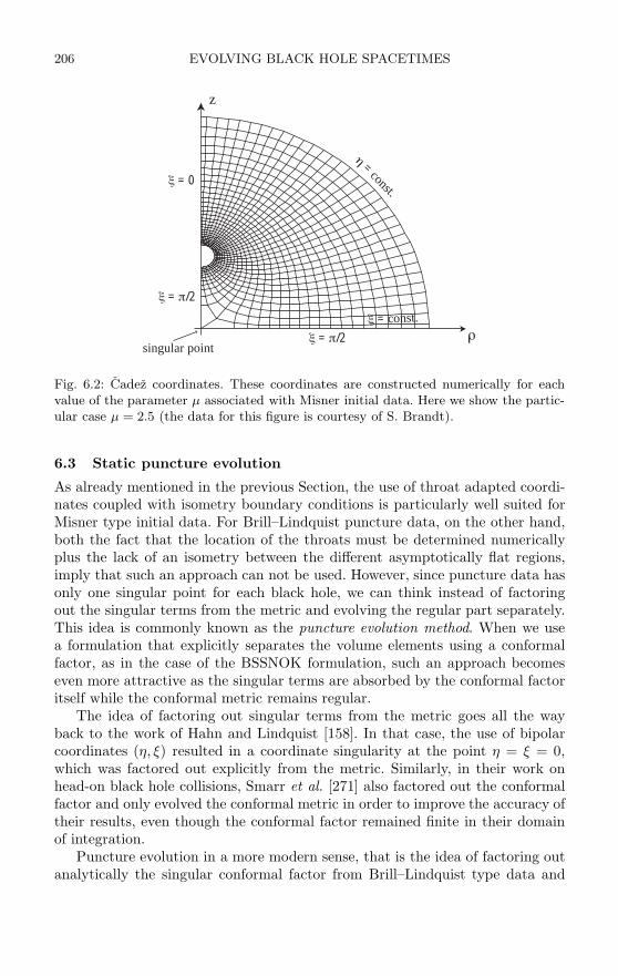
206 EVOLVING BLACK HOLE SPACETIMES
z
= const.
= const.
= 0
= /2
= /2
singular point
Fig. 6.2: Cadez coordinates. These coordinates are constructed numerically for eachvalue of the parameter µ associated with Misner initial data. Here we show the partic-ular case µ = 2.5 (the data for this figure is courtesy of S. Brandt).
6.3 Static puncture evolution
As already mentioned in the previous Section, the use of throat adapted coordi-nates coupled with isometry boundary conditions is particularly well suited forMisner type initial data. For Brill–Lindquist puncture data, on the other hand,both the fact that the location of the throats must be determined numericallyplus the lack of an isometry between the different asymptotically flat regions,imply that such an approach can not be used. However, since puncture data hasonly one singular point for each black hole, we can think instead of factoringout the singular terms from the metric and evolving the regular part separately.This idea is commonly known as the puncture evolution method. When we usea formulation that explicitly separates the volume elements using a conformalfactor, as in the case of the BSSNOK formulation, such an approach becomeseven more attractive as the singular terms are absorbed by the conformal factoritself while the conformal metric remains regular.
The idea of factoring out singular terms from the metric goes all the wayback to the work of Hahn and Lindquist [158]. In that case, the use of bipolarcoordinates (η, ξ) resulted in a coordinate singularity at the point η = ξ = 0,which was factored out explicitly from the metric. Similarly, in their work onhead-on black hole collisions, Smarr et al. [271] also factored out the conformalfactor and only evolved the conformal metric in order to improve the accuracy oftheir results, even though the conformal factor remained finite in their domainof integration.
Puncture evolution in a more modern sense, that is the idea of factoring outanalytically the singular conformal factor from Brill–Lindquist type data and
6.3 STATIC PUNCTURE EVOLUTION 207
evolving only the regular conformal metric in all 3, was first used by Anninoset al. in 1994 [25] for a single Schwarzschild black hole. In that reference the punc-ture idea was arrived at empirically by using a code that was originally designedto follow the approach of Smarr et al. that consisted of imposing an isometrycondition at the throat and at the same time factoring out the conformal factor,and then simply turning off the isometry boundary condition and evolving theconformal metric everywhere. In 1997 Brugmann [82] proposed puncture evolu-tions as a general method for the evolution of black hole spacetimes constructedwith a conformally flat metric and Bowen–York extrinsic curvature (i.e. punctureinitial data). The idea was later described in detail by Alcubierre et al. in [13],both for the ADM and BSSNOK formulations of the evolution equations. Sincethe BSSNOK formulation already separates out the volume elements from theconformal metric, it is perhaps more natural to discuss puncture evolutions inthis context.
Starting from the BSSNOK rescaling of the spatial metric:
γij := e−4φγij , (6.3.1)
we further split the conformal factor as
φ = φ + ln ψBL , (6.3.2)
where ψBL is the singular Brill–Lindquist conformal factor. For pure Brill–Lindquist type data initially we will have φ(t = 0) = 0, but for more generalpuncture data the initial conformal factor has an extra regular piece so thatφ(t = 0) = 0 (see Chapter 3). During the subsequent evolution, the regularpart of the conformal factor φ is evolved, but the singular part is kept constantin time. Terms in the evolution equations that make reference to the singularpiece of the conformal factor or its derivatives are calculated analytically. Sincethe singular piece of the conformal factor is kept constant in time, it is perhapsbetter to refer to this method as the static puncture evolution method.
We can argue that it is possible to obtain regular evolutions using this ap-proach by examining the evolution equations for the geometric quantities andthe gauge conditions close to a puncture. For simplicity, let us assume that wehave a single puncture located at the origin with zero linear momentum andspin, and consider the limit r → 0 (in the more general case the analysis ismore complicated but the results are similar). For the conformal factor we haveψBL = O(1/r) initially, and the different BSSNOK quantities will have the fol-lowing initial behavior and assumed subsequent evolution:
φ = O(1) → O(1) , (6.3.3)γrr = O(1) → O(1) , (6.3.4)K = 0 → O(r2) , (6.3.5)
Arr = 0 → O(r2) , (6.3.6)Γr = 0 → O(r) . (6.3.7)
208 EVOLVING BLACK HOLE SPACETIMES
Assume furthermore that the initial lapse is α = O(1), and the shift is purelyradial at the punctures with βr = O(r). Notice also that first derivatives of O(1)quantities are O(r) and second derivatives are again order O(1). The BSSNOKevolution equations (2.8.9), (2.8.10), (2.8.11), (2.8.12), and (2.8.25) can then beshown to imply the following behavior near the puncture
∂tφ = O(1) + O(r2) , (6.3.8)∂tγrr = O(1) + O(r2) , (6.3.9)∂tK = O(r2) + O(r4)(O(1) + O(r2) + r O(∂rφ)) , (6.3.10)
∂tArr = O(r2) + O(r4)(O(1) + O(r2) + r O(∂rφ)
+ O(∂2rφ) + O(∂rφ)2)
, (6.3.11)
∂tΓr = O(r) + O(r3) + O(r2)O(∂rφ) , (6.3.12)
where we have kept the explicit dependence on derivatives of φ. If the assumptionabout the behavior of the different quantities during evolution is to hold for alltimes, then we must clearly say something about the derivatives of the conformalfactor φ. Since we are assuming that φ is regular, we will have
φ = O(ln r) , ∂rφ = O(1/r) , ∂2rφ = O(1/r2) . (6.3.13)
Substituting this into the above expressions we see that it is compatible withour assumptions, so that to leading order we have
∂tφ = O(1) , (6.3.14)∂tγrr = O(1) , (6.3.15)∂tK = O(r2) , (6.3.16)
∂tArr = O(r2) , (6.3.17)∂tΓr = O(r) . (6.3.18)
Notice, in particular, that K, Aij and Γi will remain zero at the puncture. Incontrast, φ and the conformal metric γij will evolve at the puncture for non-zeroshift, but will remain at their initial values if the shift vanishes or if it behavesas O(r3) instead of O(r).
In the previous analysis we have assumed that the initial lapse is α = O(1),but we can start instead the evolution with a lapse of the form α = O(rn) withn an even positive number (a “pre-collapsed” lapse). In that case the abovecounting arguments will change for vanishing shift, but they will remain thesame if βr = O(r) because the shift terms will dominate.
The static puncture evolution method allows us to deal with the infinities inthe spatial metric in a clean and efficient way. Nevertheless, it has a series ofdisadvantages. From a purely numerical point of view, the infinity still exists inthe static conformal factor, so we must be careful to avoid placing a grid point
6.4 SINGULARITY AVOIDANCE AND SLICE STRETCHING 209
directly at the puncture. In practice, the numerical grid is set up in such a waythat the puncture lies between grid points, i.e. the puncture is staggered. Still,as resolution is increased it is clear that we will have to deal with larger andlarger values of the conformal factor, so that convergence near the puncture willnot be achieved.61 Other more serious effects are related to the fact that sincethe singular conformal factor is static, we are connected at all times with theother asymptotic infinities.
Perhaps the worst disadvantage of this approach, however, is the fact thathaving a static singular term implies that the punctures can not move by con-struction, so that the black hole horizons must always surround the originalposition of the puncture, even when the individual black holes have non-zerolinear momentum. This is really a serious drawback, as it forces us to use co-ordinate systems that follow the motion of the individual black holes so thatthey remain at an approximately fixed position in coordinate space. For binaryblack holes in orbiting configurations, for example, this implies that we mustuse a coordinate system that is corotating with the black holes. Still, the staticpuncture approach has been used successfully for the simulation of the grazingcollision of two black holes [7, 82], and also of orbiting black holes with corotatingcoordinates [12, 110].
The static puncture method has been recently superseded by an approachthat allows the punctures to move, resulting in much more accurate and sta-ble simulations of black hole spacetimes. We will discuss this moving puncturemethod in Section 6.6 below.
6.4 Singularity avoidance and slice stretching
When we use initial data of Misner or Brill–Lindquist type, the singularitiespresent are purely coordinate singularities. The physical singularity associatedwith the black holes is not present in the initial data. During evolution, however,the physical singularity will be rapidly approached unless our slicing conditionis chosen in such a way as to avoid the singularity. The issue of singularityavoidance was already mentioned in Chapter 4 when we discussed different slicingconditions, so here we will just summarize the main results.
The simplest possible slicing condition, namely geodesic slicing which corre-sponds to choosing α = 1 during the whole evolution, has the problem that itwill rapidly encounter the physical singularity of the black hole. For example, inthe case of a single Schwarzschild black hole, the isotropic initial data touchesthe horizon but does not penetrate inside it. The time to reach the singularitywhen using geodesic slicing will then coincide with the free-fall time for an ob-server initially at rest at the Schwarzschild horizon, which can be easily foundto be t = πM .
61Empirical experience shows, however, that this lack of convergence does not leak out ofthe black hole horizon. In fact, it usually does not extend more than a few grid points awayfrom the puncture itself.
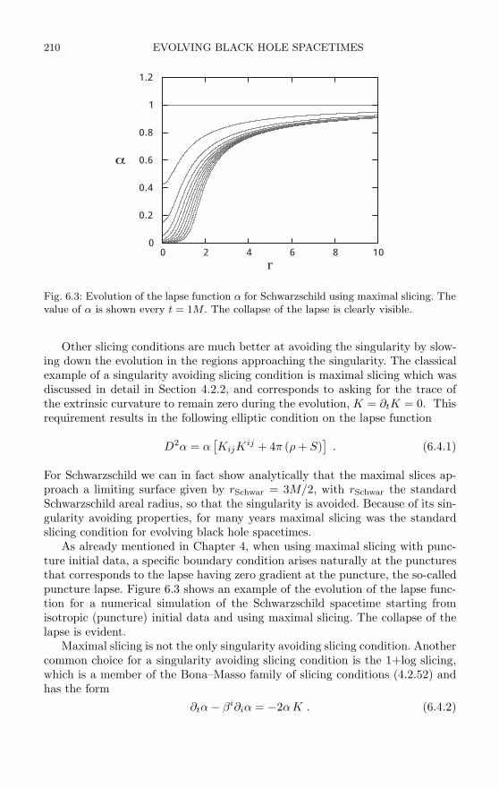
210 EVOLVING BLACK HOLE SPACETIMES
0
0.2
0.4
0.6
0.8
1
1.2
0 2 4 6 8 10r
Fig. 6.3: Evolution of the lapse function α for Schwarzschild using maximal slicing. Thevalue of α is shown every t = 1M . The collapse of the lapse is clearly visible.
Other slicing conditions are much better at avoiding the singularity by slow-ing down the evolution in the regions approaching the singularity. The classicalexample of a singularity avoiding slicing condition is maximal slicing which wasdiscussed in detail in Section 4.2.2, and corresponds to asking for the trace ofthe extrinsic curvature to remain zero during the evolution, K = ∂tK = 0. Thisrequirement results in the following elliptic condition on the lapse function
D2α = α[KijK
ij + 4π (ρ + S)]
. (6.4.1)
For Schwarzschild we can in fact show analytically that the maximal slices ap-proach a limiting surface given by rSchwar = 3M/2, with rSchwar the standardSchwarzschild areal radius, so that the singularity is avoided. Because of its sin-gularity avoiding properties, for many years maximal slicing was the standardslicing condition for evolving black hole spacetimes.
As already mentioned in Chapter 4, when using maximal slicing with punc-ture initial data, a specific boundary condition arises naturally at the puncturesthat corresponds to the lapse having zero gradient at the puncture, the so-calledpuncture lapse. Figure 6.3 shows an example of the evolution of the lapse func-tion for a numerical simulation of the Schwarzschild spacetime starting fromisotropic (puncture) initial data and using maximal slicing. The collapse of thelapse is evident.
Maximal slicing is not the only singularity avoiding slicing condition. Anothercommon choice for a singularity avoiding slicing condition is the 1+log slicing,which is a member of the Bona–Masso family of slicing conditions (4.2.52) andhas the form
∂tα − βi∂iα = −2αK . (6.4.2)

6.4 SINGULARITY AVOIDANCE AND SLICE STRETCHING 211
0
0.2
0.4
0.6
0.8
1
1.2
0 2 4 6 8 10r
Fig. 6.4: Evolution of the lapse function α for Schwarzschild using 1+log slicing. Thevalue of α is shown every t = 1M . Notice how the lapse remains equal to one at thepuncture and large gradients develop.
The 1+log slicing condition has been found to be very robust in black holeevolutions. It is also much easier to solve than maximal slicing, and becauseof this it has supplanted maximal slicing in recent years. There is, however,an important point to keep in mind when using 1+log slicing with puncturedata. Since 1+log slicing is a hyperbolic slicing condition, it has a finite speedof propagation given by v = α
√2γrr = α
√2γrr/ψ2. At the puncture ψ diverges,
so the speed of propagation vanishes (this reflects the fact that the puncture isan infinite proper distance away). As a result of this, for standard 1+log slicingthe lapse will collapse in the region around the throat of the wormhole, but willremain equal to one both at infinity and at the puncture location. Having thelapse remain equal to one at the puncture will cause extremely large gradients todevelop close to the puncture that can cause the numerical simulation to fail.62
This phenomenon can be clearly seen in Figure 6.4, which shows the evolutionof the lapse function for a numerical simulation of the Schwarzschild spacetimestarting from puncture initial data and using the 1+log slicing.
This problem of 1+log slicing with puncture data can be cured in a numberof different ways. First, we can simply ignore the region close to the puncture andcut it from the simulation using so-called excision techniques (see Section 6.5).Another possibility is to modify the 1+log condition so that the speed of prop-agation of signals becomes infinite in physical space, while remaining finite incoordinate space. This can be done by changing the 1+log condition to
62Depending on the numerical method used, we can find instead that the numerical dissipa-tion is so strong that these large gradients force the lapse to collapse at the puncture. But thisis a purely numerical artifact.

212 EVOLVING BLACK HOLE SPACETIMES
∂tα = βi∂iα − 2αψm K , (6.4.3)
with m > 0. A natural choice is m = 4, in which case the speed of propa-gation becomes finite at the puncture. Yet another possibility is to keep theoriginal form of the 1+log slicing condition, but start the simulation with a“pre-collapsed” lapse that is already zero at the puncture. We can choose, forexample, α(t = 0) = 1/ψn with n ≥ 2, which will result in an initial lapse that iszero at the puncture and also has zero gradient. Choosing n = 2 has the advan-tage that the initial lapse has the same limit for r → ∞ as the lapse of the staticSchwarzschild metric in isotropic coordinates α = (1 − M/2r)/(1 + M/2r).
The use of a pre-collapsed initial lapse has recently become the standard inblack hole simulations. In particular, the choice n = 4 seems to be required in thecase where we have spinning punctures, for which the initial extrinsic curvaturediverges as 1/r3.
There is a phenomenon related to singularity avoidance that can also causeproblems for black hole simulations. Since time freezes inside the black hole butkeeps advancing outside, the spatial slices become distorted, giving rise to thephenomenon of slice stretching which results in a rapid growth of the radialmetric component and the development of large gradients near the throat of theblack hole. We have already discussed this phenomenon in Chapter 4, where wementioned that it is in fact a combination of two separate effects, one of themrelated to the differential infall of coordinate observers close to the black hole, andthe other the result of the slices “wrapping” around the singularity. Figure 6.5shows an example of the slice stretching effect for a numerical simulation of theSchwarzschild spacetime using maximal slicing. The figure shows the evolutionof the conformal radial metric component γrr = γrr/ψ4. From the figure we canclearly see how the metric grows rapidly in the region around the horizon of theblack hole.
Historically, there have been two main strategies to avoid slice stretching. Onestrategy is again to simply ignore what happens inside the horizon by excisingthe black hole interior. The second strategy has involved the use of a shift vectorto counter the effects of slice stretching. For some time there was the hope thatshift conditions such as minimal distortion (4.3.14) would suffice to cure slicestretching, but early numerical simulations of Schwarzschild seemed to indicatedthat this was not the case [55]. In those simulations, the evolutions with no shiftresulted in the familiar growth of the radial metric component γrr in the regionaround the horizon of the black hole. Evolutions using a minimal distortion shift,on the other hand, did indeed eliminate the growth in γrr close to the horizon,but at the price of producing an even larger growth in the region close to thethroat. With hindsight, it is clear why in such simulations the shift conditionfailed to cure slice stretching. We must bear in mind the fact that all the shiftvector can do is move the coordinate lines around, but these coordinate linesmust come from somewhere. For a black hole evolved in isotropic coordinates
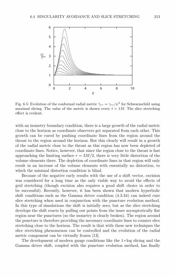
6.4 SINGULARITY AVOIDANCE AND SLICE STRETCHING 213
0
1
2
3
4
5
6
0 2 4 6 8 10r
rr
Fig. 6.5: Evolution of the conformal radial metric γrr = γrr/ψ4 for Schwarzschild usingmaximal slicing. The value of the metric is shown every t = 1M . The slice stretchingeffect is evident.
with an isometry boundary condition, there is a large growth of the radial metricclose to the horizon as coordinate observers get separated from each other. Thisgrowth can be cured by pushing coordinate lines from the region around thethroat to the region around the horizon. But this clearly will result in a growthof the radial metric close to the throat as this region has now been depleted ofcoordinate lines. Notice, however, that since the region close to the throat is fastapproaching the limiting surface r = 3M/2, there is very little distortion of thevolume elements there. The depletion of coordinate lines in that region will onlyresult in an increase of the volume elements with essentially no distortion, towhich the minimal distortion condition is blind.
Because of the negative early results with the use of a shift vector, excisionwas considered for a long time as the only viable way to avoid the effects ofgrid stretching (though excision also requires a good shift choice in order tobe successful). Recently, however, it has been shown that modern hyperbolicshift conditions such as the Gamma driver condition (4.3.34) can indeed cureslice stretching when used in conjunction with the puncture evolution method.In this type of simulations the shift is initially zero, but as the slice stretchingdevelops the shift reacts by pulling out points from the inner asymptotically flatregion near the punctures (so the isometry is clearly broken). The region aroundthe puncture is therefore providing the necessary coordinate lines to counter slicestretching close to the horizon. The result is that with these new techniques theslice stretching phenomenon can be controlled and the evolution of the radialmetric component can be virtually frozen [13].
The development of modern gauge conditions like the 1+log slicing and theGamma driver shift, coupled with the puncture evolution method, has finally
214 EVOLVING BLACK HOLE SPACETIMES
allowed the use of singularity avoiding slicings without the negative effects ofslice stretching, and this has resulted in the possibility of having long-lived andaccurate evolutions of black hole spacetimes.
6.5 Black hole excisionWhen evolving black hole spacetimes we are mostly interested in studying physi-cal effects outside of the black hole itself, such as for example the orbital dynamicsof the black holes and the gravitational wave signal emitted to infinity. Since theblack hole horizon is a causal boundary, it is clear that whatever happens insidethe black hole can not affect the physics outside. This observation gave rise tothe idea of cutting or excising the black hole interior from the simulations alto-gether, thus eliminating the need to deal with the singularities present inside theblack hole, either physical or coordinate, and also cleanly solving the problemsassociated with punctures, singularity avoidance and slice stretching. Black holeexcision was first attempted successfully by Seidel and Suen in spherical sym-metry in 1992 [261], and was later studied in more detail by Anninos et al. [26].However, the original idea has been attributed by Thornburg [284, 285] to asuggestion by Unruh from 1984.63
Black hole excision in fact consists of two separate ingredients: First, we placea boundary inside the black hole and excise its interior from the computationaldomain. Second, we use a non-zero shift vector that keeps the horizon roughlyin the same coordinate location during the evolution. Since no information canleave the interior of the black hole, excision should have no effect on the physicsoutside. Ideally, we would like to know the position of the event horizon whichmarks the true causal boundary, but the global character of its definition meansthat in principle we can only locate it once the whole evolution of the spacetimeis known. The apparent horizon, on the other hand, can be located on everytime slice and is guaranteed to be inside the event horizon (assuming cosmiccensorship holds). In practice we therefore needs to find the apparent horizonand excise a region inside it.
Over the years, a number of different excision techniques have been developedby different researchers, with limited degrees of success. Early on it was realizedthat in order for excision to work, and for the black hole horizon to remain withan approximately fixed size in coordinate space, a superluminal shift vector wasrequired. It is in fact easy to see why this should be so. Consider for a momenta point with fixed spatial coordinates xi directly on the black hole horizon. Ifthe shift is zero, this point will move on a timelike trajectory (the normal to thehypersurfaces), so at any later time it must be well inside the black hole, butsince it still has the same spatial coordinates this means that the horizon musthave moved outward in coordinate space (in other words, the black hole swallowsthe coordinate lines). So for the horizon to remain fixed in coordinate space we
63In the early literature the name “apparent horizon boundary condition” is used instead ofthe more modern name of “black hole excision” [26, 261]. This older name is now consideredinadequate as no boundary condition is placed at the apparent horizon directly.

6.5 BLACK HOLE EXCISION 215
need an outward pointing shift vector to counter this effect. In fact, the shiftvector must be such that the coordinate lines move out at the speed of light atthe horizon, and faster than light inside the horizon. This is, of course, no causefor alarm as we are only talking about the “motion” of the coordinates and notany physical effect.
As it turns out, some simple numerical methods become unstable when theshift is superluminal, so in the early 1990s numerical techniques known as “causaldifferencing” [261] and “causal reconnection” [20] where developed that tried totilt the computational molecules in order for them to follow the physical light-cones. However, later on it was realized that when using hyperbolic formulationsof the evolution equations this was unnecessary, and quite standard numericaltechniques should be able to cope with superluminal shifts as long as the CFLstability condition remains satisfied (see Chapter 9).64 Moreover, when usinghyperbolic formulations of the evolution equations we find that inside the blackhole all characteristics move inward, so there is no need for a boundary conditionon the excision surface as all the necessary causal information is in fact known.In more geometric terms, the excision surface is spacelike, so it is not a boundaryas such, but rather a “time” at which we simply stop integrating – see Figure 6.6(a possible exception to this would be the existence of gauge modes that movefaster than light and that could have incoming characteristics at the excisionsurface, but we can always choose a gauge that does not behave in this way).
Though black hole excision has been successful in spherical symmetry [26,196, 173, 151, 253, 254, 256, 261], it has been very difficult to implement with a3+1 approach in three dimensions [25, 81, 104, 107, 286, 296] (black hole excisionusing a characteristic formulation, on the other hand, has been very successful in3D, allowing stable evolutions of perturbed black holes for essentially unlimitedtimes [147]). The main problem is related to the fact that the excision surface istypically of spheroidal shape and this is hard to represent on a Cartesian grid. Itis therefore difficult to even define at a given point on the excision surface whatis the “outward” direction. This inevitably leads to the use of extrapolationsin several directions in order to be able to do the finite differencing, and thisextrapolation is typically very unstable. One important development in this areawas the introduction of so-called simple excision techniques [10]. The originalidea behind such techniques was to excise a simple surface in Cartesian coordi-nates (e.g. a cube), and then to apply very simple boundary conditions on thatsurface, in particular simply copying the values of all dynamical variables ontothe excision cube from the point directly adjacent to it. Such techniques havehave later been generalized to the case of more complicated excision surfaces (so-called “lego-spheres”), and have allowed the simulation of black hole collisionsfor some limited times [12, 15]. Still, excision techniques in Cartesian grids have
64A common practice is to use one-sided differences in the shift advection terms (terms involv-ing βi∂i) to improve accuracy and stability, this being the only place where any considerationabout causality enters the numerical code (i.e. the direction of the tilt of the light-cones).
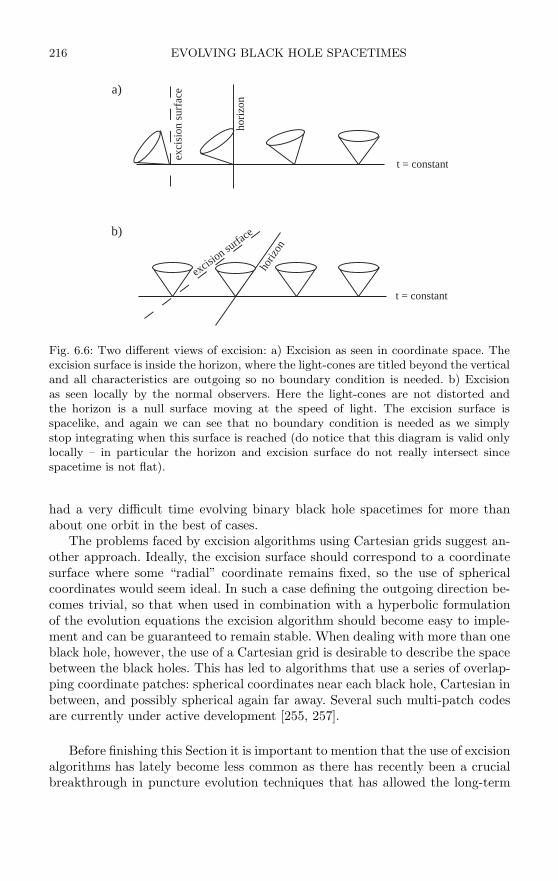
216 EVOLVING BLACK HOLE SPACETIMES
hori
zon
exci
sion
sur
face
t = constant
a)
b)
t = constant
horiz
onex
cision su
rface
Fig. 6.6: Two different views of excision: a) Excision as seen in coordinate space. Theexcision surface is inside the horizon, where the light-cones are titled beyond the verticaland all characteristics are outgoing so no boundary condition is needed. b) Excisionas seen locally by the normal observers. Here the light-cones are not distorted andthe horizon is a null surface moving at the speed of light. The excision surface isspacelike, and again we can see that no boundary condition is needed as we simplystop integrating when this surface is reached (do notice that this diagram is valid onlylocally – in particular the horizon and excision surface do not really intersect sincespacetime is not flat).
had a very difficult time evolving binary black hole spacetimes for more thanabout one orbit in the best of cases.
The problems faced by excision algorithms using Cartesian grids suggest an-other approach. Ideally, the excision surface should correspond to a coordinatesurface where some “radial” coordinate remains fixed, so the use of sphericalcoordinates would seem ideal. In such a case defining the outgoing direction be-comes trivial, so that when used in combination with a hyperbolic formulationof the evolution equations the excision algorithm should become easy to imple-ment and can be guaranteed to remain stable. When dealing with more than oneblack hole, however, the use of a Cartesian grid is desirable to describe the spacebetween the black holes. This has led to algorithms that use a series of overlap-ping coordinate patches: spherical coordinates near each black hole, Cartesian inbetween, and possibly spherical again far away. Several such multi-patch codesare currently under active development [255, 257].
Before finishing this Section it is important to mention that the use of excisionalgorithms has lately become less common as there has recently been a crucialbreakthrough in puncture evolution techniques that has allowed the long-term
6.6 MOVING PUNCTURES 217
simulation of binary black hole spacetimes without the need to excise the blackhole interior (see the following Section).
6.6 Moving puncturesIn Section 6.3 we described the basic ideas behind the static puncture evolutionmethod. This method allows us to handle the infinities associated with punctureinitial data in a clean way, but it has one major disadvantage, namely that byfactoring out the infinities analytically and keeping them static it forces thepunctures to remain at a fixed coordinate location even for black holes that havenon-zero linear momentum.
Very recently there has been a true breakthrough in black hole simulationsby taking some of the basic ideas of the puncture evolution method while at thesame time allowing the punctures to evolve. This simple idea has finally allowedthe accurate simulation of binary black holes for multiple orbits, with the blackholes moving through the grid as we would expect, instead of remaining gluedin a fixed position as the static puncture evolution method required. The idea ofevolving the punctures was arrived at independently, using slightly different butequivalent methods, by Campanelli et al. [92, 93] and Baker et al. [44, 45].65
6.6.1 How to move the puncturesThe moving puncture idea starts from the BSSNOK formulation, as in the staticpuncture approach, but now the singular part of the conformal factor is notfactored out. The dynamical conformal factor φ = lnψ then has a logarithmicsingularity which is directly evolved. The approaches of Campanelli et al. andBaker et al. differ on how this singularity is evolved in practice.
The approach of Baker et al. is to simply evolve φ directly. Notice that as longas we make sure that initially the point r = 0 does not correspond to a grid point(the puncture is staggered) no actual infinities will be present on the numericalgrid. Of course, we could worry about the effect of taking numerical derivativesacross the logarithmic singularity in φ. Empirically we find that such derivatives,though certainly introducing large numerical errors, nevertheless result in stableevolutions. Moreover, the numerical errors associated with taking derivativesacross the puncture do not seem to leak out of the black hole and in fact onlyaffect the region immediately adjacent to the puncture.
In contrast, Campanelli et al. define a new function χ through
χ = ψ−4 = e−4φ . (6.6.1)
65One should mention the fact that the first simulation of binary black holes through sev-eral orbits with the black holes moving through the grid was in fact done by Pretorius usingan approach based on evolving the full 4-metric of the spacetime in generalized harmonic co-ordinates [231, 232, 233]. This method seems to be extremely robust and powerful and it isactively being used by several numerical relativity groups, but as it is not directly based ona 3+1 approach we will not discuss it here. Both the approach of Pretorius and the movingpuncture method where developed within a year of each other in 2004–05, showing the tremen-dous amount of progress that the field of black hole simulations has seen within the last fewyears.
218 EVOLVING BLACK HOLE SPACETIMES
The evolution equation for χ follows from that for φ and has the form
∂tχ − βi∂iχ =23χ(αK − ∂iβ
i)
. (6.6.2)
Notice that while ψ has a 1/r pole at the puncture, χ is instead O(r4) at thepuncture. We then do not have to differentiate an infinite quantity at the punc-ture, but rather a C4 quantity. Still, since there will be explicit divisions by χ inthe evolution equations, we must ensure that χ is never exactly zero (in practicewe can set the value of χ to some very small positive number whenever it eithergets too close to zero or becomes negative due to numerical error).
Of course, evolving the puncture directly does not immediately imply that itwill move across the grid. From the discussion in Section 6.3 we can see that forvanishing shift the punctures will simply not evolve. We therefore need to havea good choice of gauge conditions. Moving puncture approaches typically use a1+log slicing condition
∂tα − βi∂iα = −2αK , (6.6.3)
together with a shift vector of the Gamma driver family (4.3.34) of the form
∂0βi = Bi , ∂0B
i =34
∂0Γi − ηBi . (6.6.4)
Notice that no power of the lapse is present in the coefficient in front of ∂0Γi, aswe want the shift to evolve at the puncture where the lapse will collapse to zero.The operator ∂0 is taken to be equal to ∂t in some approaches and to ∂t−βi∂i inothers (and even different combinations are used in the different terms). Noticethat having a non-zero shift at the position of the puncture is precisely whatallows it to move. The position of the puncture xi
p can be tracked by integratingthe equation of motion66
dxip
dt= −βi
(xj
p
). (6.6.5)
The shift is typically chosen to vanish initially, but the Gamma driver condi-tion rapidly causes the shift to evolve in such a way that it not only counteractsthe longitudinal slice stretching effect, but for orbiting black holes it also auto-matically acquires a tangential component that allows the punctures to orbit oneanother. Also, because of the problem of the lack of collapse of the 1+log lapse atthe puncture discussed in the previous Section, the initial lapse is usually takento be of a pre-collapsed type α(t = 0) = ψ−n, with n equal to 2 or 4.
Both the φ-method and the χ-method have been shown empirically to leadto robust and stable simulations of black hole spacetimes, allowing us to followbinary black holes for several orbits through the merger and ring-down, and to
66In practice, this equation does not need to be integrated very accurately, since with the shiftconditions typically used (i.e. the Gamma driver shift) the position of the puncture behavesas an attractor.
6.6 MOVING PUNCTURES 219
extract accurate gravitational waves, with evolution times that can last for manyhundreds of M ’s. A recent review of the moving puncture approach can be foundin [83].67
6.6.2 Why does evolving the punctures work?
The fact that moving puncture evolutions work can seem at first sight to bequite surprising. After all, we are “moving” through the numerical grid a pointthat corresponds to another infinitely far away, asymptotically flat region, andat which the conformal factor diverges. The sole idea of taking finite differencesacross this singular point should be enough to send any experienced numericalanalyst into a panic attack. Clearly, we would expect numerical errors to getworse close, the puncture as the resolution is increased, destroying any chanceof convergence. These errors should then quickly contaminate the entire domainof integration, rendering the whole numerical solution useless. Indeed, it wasprecisely this fear of dealing numerically with infinities that gave rise to theideas of black hole excision and static puncture evolutions in the first place. Butnumerical experiments have shown that the fears were exaggerated, and that sim-ulations involving moving punctures not only do converge but can also be highlyaccurate. Of course, empirical evidence aside, we would like to understand thereason why evolving the punctures works. The problem can in fact be separatedin two distinct issues: First, from the point of view of numerical analysis, whyis it that the formally infinite errors near the puncture do not contaminate thewhole solution? And second, from a point of view of general relativity, how is itpossible that near each puncture the lapse and shift conditions seem to drive thesolution into a stationary situation?
The first question has in fact not been tackled formally yet, but there is aheuristic argument as to why numerical errors do not contaminate the wholesolution. First, we must remember that the punctures are inside the black holehorizons, so that the effects of the numerical errors would have to propagatefaster than light to contaminate the exterior solution. As puncture evolutions aretypically done using hyperbolic formulations it is clear that errors will propagateat a finite speed. If this speed is smaller than the speed of light the errors shouldnot be able to “escape” from the black hole. Moreover, as we will see below, itturns out that at late times the puncture is in fact not at asymptotic infinity, butrather truly inside the black hole, so that all characteristics near the puncturepoint inwards, and the errors can be expected to remain “trapped” close tothe puncture. Of course, this heuristic explanation is not sufficient as it is clearthat when using a centered numerical scheme (as is usually done) numericalerrors must propagate to the whole grid regardless of the sign of the physicalcharacteristics. So what is really needed is a formal proof that shows that as
67Systematic studies have also shown that extremely high numerical resolution is requiredto evolve the black holes accurately. Because of this, modern algorithms use fourth orderdifferencing in both space and time, plus some form of mesh refinement, to allow high resolutionclose to each of the black holes while keeping the outer boundaries as far away as possible.
220 EVOLVING BLACK HOLE SPACETIMES
resolution is increased, the effect of these errors leaking out of the black holebecome smaller and smaller so that the simulation converges. At the time ofwriting this book such an analysis has not yet been done, but in some simplifiedsystems it might not be so difficult to address.
There has been more progress on the second issue regarding the final sta-tionary state reached near each puncture. Recent work by Hannam et al. [159]has shown that, at least in the case of Schwarzschild, the 1+log slicing conditiontogether with a Gamma driver shift condition does indeed allow us to find anexplicitly time independent form of the Schwarzschild metric that penetrates thehorizon and corresponds to the final state of the “evolving puncture” simulationsto within numerical error. The surprising result has been that as the simulationproceeds the numerical puncture ceases to correspond to another asymptoticallyflat region and moves to a minimal surface inside the black hole. Also, the singu-larity in the conformal factor changes character. Without going into the detailsof their argument, Hannam et al. show that once the stationary state is reached,the lapse and conformal factor behave near the puncture as
α ∼ r , ψ ∼ 1/√
r , (6.6.6)
which is in contrast with the initial conformal factor of the isometric initial dataψ ∼ 1/r, and the initial pre-collapsed lapse typically chosen for these simulationsα ∼ r2. More interesting is the fact that since the area of spheres close to thepuncture goes as r2ψ4, we now find that at the puncture itself this area remainsfinite, so that the puncture no longer corresponds to asymptotic infinity. Forstandard 1+log slicing we can in fact show that the puncture corresponds to acylinder with areal radius R0 ∼ 1.31M < 2M , i.e. well inside the black holehorizon (the puncture, however, is still an infinite proper distance away from thehorizon).
We can ask how it is possible that a slice that initially reaches the otherasymptotic infinity ends up instead reaching a cylinder inside the black hole.What is happening is that, as the evolution proceeds, the slicing condition causesthe throat of the Einstein-Rosen bridge to collapse toward the limiting cylinderwith radius R0, while at the same time the shift condition makes the throatapproach the puncture exponentially in coordinate space. After a relatively shorttime, the throat is less that one grid point away from the puncture, so the wholespace between the throat and the inner asymptotic infinity is squeezed into aregion that can simply not be resolved numerically, and in practice the puncturecan now be assumed to correspond to the throat itself.
As a final comment, the fact that we start with two asymptotically flat regionsbut end up with a single region that reaches an inner throat at the punctureimmediately raises the possibility of constructing initial data that already hasthis final topology, and using it instead of the standard Brill–Lindquist type data.This is an issue that will no doubt receive much attention in the near future.
6.7 APPARENT HORIZONS 221
6.7 Apparent horizons
Being able to evolve a black hole spacetime in a stable and consistent way, thoughclearly crucial, is not enough. We would also like to be able to extract physical in-formation from the numerically generated spacetime. Such physical informationincludes both far field studies such as the extraction of the emitted gravitationalwaves (see Chapter 8), and near field studies related to the dynamics of theblack hole horizons and the extraction of physical quantities such as the blackhole mass and spin. Locating black hole horizons is also crucial if we are usingan approach based on singularity excision, since in that case we need to be surethat the region excised from the computational domain is safely inside the blackhole.
There are in fact two different types of horizon associated with black holes.On the one hand, we define the event horizon as the boundary between null linesthat “escape” to infinity and those that fall back into the black hole and hit thesingularity instead. Since an event horizon is defined in a global way we need inprinciple to know the full evolution of the spacetime (or a significant part of it)in order to locate it, which means that it can not be used as an indicator of thepresence and location of a black hole during an evolution. Apparent horizons, onthe other hand, are defined locally as the outermost marginally trapped surfaceon a given spatial hypersurface, that is, a closed two-dimensional surface S suchthat the expansion of outgoing null geodesics orthogonal to S is zero everywhere.An important property of apparent horizons is the fact that, if the cosmic censor-ship conjecture holds and the null energy condition is satisfied, then an apparenthorizon implies the existence of an event horizon exterior to it, or coincidentwith it in the stationary case.
Apparent horizons can be located during an evolution on each spatial hyper-surface. They are thus ideal indicators of the presence of a black hole, and can beused both to locate the black holes in order to use e.g. black hole excision tech-niques, and also to measure physical quantities associated with each black holesuch as mass and angular momentum. In order to locate apparent horizons ona given spatial hypersurface we must first derive an equation that characterizesthem.
Consider then a closed two-dimensional surface S immersed in our three-dimensional spatial hypersurface Σ. Let s be the spacelike unit outward-pointingnormal vector to S, and n the timelike unit future-pointing normal vector to Σ.We can now use these vectors to construct the outgoing null vector l as68
l = n + s . (6.7.1)
The expansion of the null lines is essentially the change in the area elements ofS along l. If we denote by hµν the two-dimensional metric on S induced by thespacetime metric gµν we will have
68The normalization of the null vector l is in fact arbitrary. Throughout most of the book wewill usually take l = ( n + s)/
√2, but here we drop the factor 1/
√2 to simplify the notation.
222 EVOLVING BLACK HOLE SPACETIMES
hµν = gµν + nµnν − sµsν . (6.7.2)
The expansion H of the outgoing null geodesics will then be
H = −12
hµν£l hµν = −12
hµν (£s hµν + £n hµν) . (6.7.3)
But £s hµν = −2Xµν, with Xµν the extrinsic curvature of S, so that
hµν£s hµν = −2 hµνXµν = −2X = −2Dmsm , (6.7.4)
with Di the three-dimensional covariant derivative in Σ. On the other hand
hµν£n hµν = hµν [£n gµν + £n nµnν − £n sµsν ]= −2hµνKµν + hµν [£n nµnν − £n sµsν ] , (6.7.5)
where Kµν is the extrinsic curvature of Σ. Using now the fact that nαnα = −1,sαsα = 1 and nαsα = 0 we find
hµν£n nµnν = hµν£n sµsν = 0 , (6.7.6)
so that
hµν£n hµν = −2 hµνKµν = −2K + 2Kmnsmsn , (6.7.7)
with K the trace of Kµν . Collecting results we finally find
H = Dmsm − K + Kmnsmsn
= (γmn − smsn) (Dmsn − Kmn) , (6.7.8)
where in the latter equality we used the fact that smsm = 1 implies smDnsm = 0.The condition for having an apparent horizon is by definition H = 0, so that
the equation that characterizes the apparent horizon takes the final form
H = Dmsm − K + Kmnsmsn = (γmn − smsn) (Dmsn − Kmn) = 0 . (6.7.9)
Notice that the condition for having a minimal (or rather extremal) surface,like the throat of a wormhole for example, is simply
Dmsm = 0 , (6.7.10)
so that for time symmetric data with Kij = 0 the apparent horizon will coincide(at least initially) with the minimal surface, i.e. with the throat of the Einstein–Rosen bridge.
6.7 APPARENT HORIZONS 223
It is often convenient to characterize an apparent horizon by assuming thatthe surface has been parameterized as a level set of some scalar function F :
F (xi) = 0 . (6.7.11)
It is then straightforward to rewrite H in terms of the function F and its deriva-tives. First, we write the unit normal vector si as
si = DiF/u , (6.7.12)
with u := |DF | = (γmnDmFDnF )1/2. Substituting this in equation (6.7.9)results, after some algebra, in
H =(
γmn − DmFDnF
u2
)(DmDnF
u− Kmn
)= 0 . (6.7.13)
Having found the equation that must be satisfied by an apparent horizon,the next step is to develop an algorithm to solve this equation. For this we willconsider the cases of spherical and axial symmetry separately since in those casesthe problem simplifies considerably. A very complete discussion of the differentalgorithms for finding apparent horizons can be found in the recent review byThornburg [287].
As a final comment, it is important to mention the fact that apparent horizonsdo not evolve in a smooth way during gravitational collapse. On the contrary,we typically find that an apparent horizon can jump discontinuously when a newlarger marginally trapped surface appears outside the earlier apparent horizon.This is typical of black hole collisions where a common apparent horizon suddenlyappears outside the individual apparent horizons.
6.7.1 Apparent horizons in spherical symmetryLet us consider first a spherically symmetric spacetime. We can write the spatialmetric quite generally in terms of spherical coordinates r, θ, φ as
dl2 = A(r, t)dr2 + r2B(r, t) dΩ2 , (6.7.14)
with A and B positive, and where dΩ2 = dθ2 + sin2 θdφ2 is the standard solidangle element. In order to obtain an expression for the expansion of the outward-pointing null geodesics we can take s as the unit radial vector: s = (1/
√A, 0, 0).
After some simple algebra the expansion H can be found to be
H =1√A
(2r
+∂rB
B
)− 2Kθ
θ , (6.7.15)
so that the condition for an apparent horizon reduces to
1√A
(2r
+∂rB
B
)− 2Kθ
θ = 0 . (6.7.16)
Notice that this should not be understood as a differential equation for the metriccoefficient B, but rather as a condition that indicates the presence of an apparenthorizon at some value of the radial coordinate r.

224 EVOLVING BLACK HOLE SPACETIMES
As an example, consider the case of a single black hole in Schwarzschildcoordinates for which we have Kθ
θ = 0, A = 1/(1 − 2M/r) and B = 1, so thatthe horizon condition becomes
2r
√1 − 2M/r = 0 ⇒ r = 2M . (6.7.17)
On the other hand, in isotropic coordinates we have Kθθ = 0 and A = B =
ψ4, with ψ = 1 + M/2r (cf. equation (1.15.28)), so that the apparent horizoncondition takes the form
1ψ2
(2r
+4 ∂rψ
ψ
)= 0 ⇒ r = M/2 . (6.7.18)
Here we must remember that the radial coordinate r in each case has a differ-ent meaning, with the isotropic and Schwarzschild radii riso and rSchwar relatedthrough rSchwar = riso (1 + M/2riso)
2, so that riso = M/2 implies rSchwar = 2M ,in agreement with the above results.
In a more general case all we need to do in order to locate an apparent horizonin spherical symmetry is to simply evaluate the expansion (6.7.15) over the wholecomputational domain and look for places where it vanishes (accuracy higherthan the grid spacing can be obtained by using linear or quadratic interpolation).The outermost zero will indicate the apparent horizon, while regions with H < 0will correspond to trapped surfaces. In some cases we can find that H vanishes atmore than one place, implying the presence of other marginally trapped surfaces,so-called inner horizons. This situation is typical of black holes formed throughgravitational collapse, where a single marginally trapped surface forms first asH becomes zero at a single point while remaining positive everywhere else. Thisinitial apparent horizon later splits into an inner and an outer horizon, with atrapped region in between. The inner horizon then moves toward a smaller radiusas the physical singularity is approached.
When dealing with black hole spacetimes represented through wormholes,however, there is a final subtlety that should be kept in mind. Although outsidethe wormhole it is clear that the direction of increasing r points outward, insidethe wormhole this is not true and the “outward” direction corresponds in fact tothat of decreasing r (we are going out on the other side). This means that if weare trying to locate an apparent horizon on the other side of the wormhole thenormal vector should instead be s = (−1/
√A, 0, 0), and the expression for the
expansion H must be changed to
H = − 1√A
(2r
+∂rB
B
)− 2Kθ
θ . (6.7.19)
6.7.2 Apparent horizons in axial symmetryConsider next the case of an axisymmetric spacetime. In this case the apparenthorizon will be a surface of revolution around the axis of symmetry. It can thenbe described in spherical coordinates as a level surface of the form
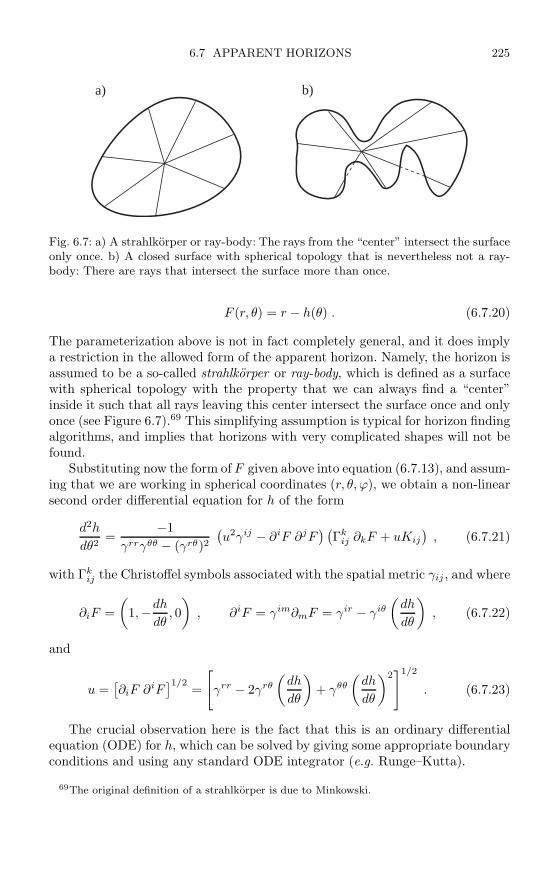
6.7 APPARENT HORIZONS 225
a) b)
Fig. 6.7: a) A strahlkorper or ray-body: The rays from the “center” intersect the surfaceonly once. b) A closed surface with spherical topology that is nevertheless not a ray-body: There are rays that intersect the surface more than once.
F (r, θ) = r − h(θ) . (6.7.20)
The parameterization above is not in fact completely general, and it does implya restriction in the allowed form of the apparent horizon. Namely, the horizon isassumed to be a so-called strahlkorper or ray-body, which is defined as a surfacewith spherical topology with the property that we can always find a “center”inside it such that all rays leaving this center intersect the surface once and onlyonce (see Figure 6.7).69 This simplifying assumption is typical for horizon findingalgorithms, and implies that horizons with very complicated shapes will not befound.
Substituting now the form of F given above into equation (6.7.13), and assum-ing that we are working in spherical coordinates (r, θ, ϕ), we obtain a non-linearsecond order differential equation for h of the form
d2h
dθ2=
−1γrrγθθ − (γrθ)2
(u2γij − ∂iF ∂jF
) (Γk
ij ∂kF + uKij
), (6.7.21)
with Γkij the Christoffel symbols associated with the spatial metric γij , and where
∂iF =(
1,−dh
dθ, 0)
, ∂iF = γim∂mF = γir − γiθ
(dh
dθ
), (6.7.22)
and
u =[∂iF ∂iF
]1/2=
[γrr − 2γrθ
(dh
dθ
)+ γθθ
(dh
dθ
)2]1/2. (6.7.23)
The crucial observation here is the fact that this is an ordinary differentialequation (ODE) for h, which can be solved by giving some appropriate boundaryconditions and using any standard ODE integrator (e.g. Runge–Kutta).
69The original definition of a strahlkorper is due to Minkowski.

226 EVOLVING BLACK HOLE SPACETIMES
The boundary conditions can be derived from the fact that the apparenthorizon should be a smooth surface. If we integrate from θ = 0 to θ = π,smoothness requires that h(θ) should have zero derivative at both boundaries,that is
∂θh = 0 , θ = 0, π . (6.7.24)
In some cases we have equatorial symmetry as well as axial symmetry, in whichcase we can stop the integration at θ = π/2 and impose the boundary condition∂θh = 0 there.
The way to find a horizon in practice is to start at some arbitrary pointr = r0 on the symmetry axis (say, a few grid points away from the origin),and integrate the second order differential equation (6.7.21) with the boundaryconditions h = r0 and ∂θh = 0 at θ = 0. When we reach θ = π (or θ = π/2for equatorial symmetry), we check whether the boundary condition ∂θh = 0is satisfied at that point to some numerical tolerance. If it is, we have foundan apparent horizon, but if it isn’t we move up along the axis and start again.If no horizon has been found as we reach the end of the axis, then no horizonexists in our spacetime. This method is usually called a shooting method in theODE literature, because we start with some initial guess at one boundary and“shoots” to the other boundary, adjusting the initial guess (we “aim better”)until we obtain the desired boundary condition on the other side (we “hit thetarget”).
6.7.3 Apparent horizons in three dimensions
As we have seen in the previous Sections, finding apparent horizons in sphericalsymmetry reduces to locating the zeros of a one-dimensional function, while inaxial symmetry it reduces to integrating an ordinary differential equation subjectto certain boundary conditions. In three dimensions, however, the problem isconsiderably more complicated. Nevertheless, a number of different algorithmsdesigned for finding apparent horizons in three dimensions have been proposedover the years. Here I will concentrate on three such algorithms and mention onlythe main ideas associated with each of them. For a more detailed description ofthe algorithms the reader is directed to the recent review by Thornburg [287](this review includes an extensive list of references of working implementationsof the different algorithms).
6.7.3.1 Minimization algorithms. Minimization algorithms for finding appar-ent horizons were among the first methods ever tried and were in fact the originalmethods used by Brill and Lindquist [79] and by Eppley [124]. The basic idea be-hind a minimization algorithm is to expand the parameterization function F (xi)in terms of some set of basis functions, and then minimize the surface integralof the square of the expansion H2 over the space of these basis functions. At anapparent horizon this integral will vanish and we will have a global minimum.Numerically, of course, the integral will never vanish exactly so we set a tolerancelevel below which a horizon is assumed to have been found.

6.7 APPARENT HORIZONS 227
A typical minimization apparent horizon finder uses a parameterization ofthe horizon of the form
F (r, θ, φ) = r − h(θ, φ) , (6.7.25)
again, assuming the horizon is a ray-body. The function h(θ, φ) in then expandedin terms of spherical harmonics as
h(θ, φ) =lmax∑l=0
l∑m=−l
al,mY l,m(θ, φ) , (6.7.26)
with al,m some constant coefficients.Given a trial function h (i.e. a trial set of al,m), we reconstruct F = r − h,
find the expansion H , and calculate the surface integral of H2. A standard min-imization algorithm can then be used to determine the values of the coefficientsal,m for which the integral reaches a minimum. Notice that we can in principlecalculate H over the entire three-dimensional grid by using finite differences inCartesian coordinates, and later interpolate it into the surface r = h(θ, φ) inorder to do the integral. This procedure is computationally expensive but verysimple to code. Alternatively, we can calculate H directly on the surface by usingfinite differencing in the angular coordinates.
Even though the idea behind minimization algorithms is straightforward,they have at least two serious drawbacks. First, the algorithm can very easilysettle on a local minimum for which the expansion is not zero, so a good initialguess is often required. Also, minimization algorithms tend to be very slow: IfN is the total number of terms in the spectral decomposition, a minimizationalgorithm requires a few times N2 evaluations of the surface integrals. Finally,minimization algorithms are only as accurate as the tolerance given, and inpractice the tolerance can not be too small since we run the risk of not findingthe horizon at all. Because of this, minimization algorithms are now rarely usedin practice.
6.7.3.2 Flow algorithms. Flow algorithms work by evolving an initial trial sur-face in some unphysical time λ in such a way that the trial surface approachesthe apparent horizon asymptotically. The basic idea behind a flow algorithm isthe following: We starts with a spherical trial surface that is considerably fur-ther out than the expected apparent horizon, and calculate the expansion Hover the whole surface which, being well outside the horizon, should be positiveeverywhere. At each point, the trial surface is now moved inward a distance pro-portional to the value of H at that point. If we have a point on the trial surfacewith coordinates xi, it will then move according to the equation
dxi
dλ= −Hsi , (6.7.27)
where si is the unit normal to the surface at that point. A flow algorithm of thistype for finding apparent horizons was first proposed by Tod in 1991 [291]. In
228 EVOLVING BLACK HOLE SPACETIMES
the case when the extrinsic curvature vanishes we have H = ∇isi, the apparent
horizon then reduces to a minimal surface and the flow method is guaranteedto converge (the method is then known as mean curvature flow). In the moregeneral case no such proof exists, but in practice flow algorithms do seem toconverge to the apparent horizon.
If we parameterize our family of surfaces as F (xi, λ) = 0, we then find
dF
dλ= ∂λF +
dxi
dλ∇iF = 0 , (6.7.28)
which using the flow equation can be reduced to
∂λF = Hsi∇iF = |∇F |H , (6.7.29)
where we have used the fact that the normal vector is given in terms of F assi = ∇iF/ |∇F |. Taking now as usual F = r−h(θ, φ), the flow equation becomes
∂λh = − |∇(r − h)|H . (6.7.30)
We can now use this equation directly to evolve the function h in the unphysicaltime λ until the right hand side vanishes and the evolution reaches a stationarystate, at which point we have found the apparent horizon.
The direct flow algorithm just described has one serious disadvantage: Whenwe write the expansion H explicitly, it turns out to be a second order ellipticoperator on the function h(θ, φ). The flow equation then has the structure ofa non-linear heat equation, so that numerical stability demands a very smalltime-step (the stability condition takes the form ∆λ ∼ (∆x)2, with x any of theangular coordinates). For a reasonably high angular resolution the algorithm canthen become too slow to use more than a few times during an evolution.
In order to improve on its speed, the basic flow algorithm can be generalizedin a number of different ways. For example, we can use implicit integrators inthe unphysical time λ (see for example [269]). Gundlach, however, has suggesteda very different way of improving flow algorithms by considering a generalizedflow equation of the form [152]
∂λh = −A(1 − BL2
)−1ρH , (6.7.31)
with ρ some scalar function constructed from Kij, gij , si, and where L2 denotes
the angular part of the flat-space Laplace operator:
L2f :=1
sin θ∂θ (sin θ ∂θ) +
1sin2 θ
∂2ϕf . (6.7.32)
The expression(1 − BL2
)−1 denotes the inverse of the operator(1 − BL2
). We
can compute this inverse explicitly by expanding the function h in terms ofspherical harmonics as in (6.7.26). Gundlach’s flow equation then becomes

6.7 APPARENT HORIZONS 229
∂λal,m = − A
1 + Bl(l + 1)(ρH)l,m . (6.7.33)
This can now be solved by forward differencing to obtain the following iterativeprocedure
a(n+1)l,m = a
(n)l,m − A
1 + Bl(l + 1)(ρH)(n)l,m . (6.7.34)
Notice that if we take ρ = |∇F |, A > 0 and B = 0 we recover the standardflow algorithm. Gundlach shows that for values of B different from zero, and forother choices of ρ, we can obtain flows that are significantly faster (essentiallybecause of the smoothing property of the (1−BL2)−1 operator), giving rise to theterm fast flow algorithms. In particular, the well known algorithm of Nakamura,Kojima and Oohara of 1984 [214] can be rewritten as a fast flow for a specificform of ρ in the limit when A = B → ∞.
Flow algorithms have one important strength and one main drawback. Theirstrength is related to the fact that they are global algorithms is the sense thatthey do not need a good initial guess in order to find the apparent horizon. Theirmain disadvantage is the fact that, even in their faster versions, they are stillconsiderably slower than the direct solvers we will discuss below (there is at leastone major exception in the flow algorithm of Meztger which uses finite elementsand is reported to be very fast [203]). However, flow algorithms are still usedby a number of different groups and their conceptual simplicity will probablyguarantee that they will remain in use for the foreseeable future.
6.7.3.3 Direct elliptic solvers. This family of algorithms takes the standardparameterization of the level surface H(r, θ, φ) = r − h(θ, φ), and interpretsthe horizon equation (6.7.13) as a non-linear second order elliptic differentialequation for the function h in the space of the two angular coordinates. Theidea is then to solve this equation using standard techniques for solving non-linear elliptic problems. Typically, we can calculate all derivatives using finitedifferences and later use Newton’s method to solve the resulting system of non-linear algebraic equations.
Many different versions of these direct elliptic solvers have been used to locateapparent horizons in three dimensions, and we will not go into the details herehere (but see Thornburg’s review for a more detailed description [287]). Thesetypes of finder have the advantage that they can be very fast indeed (for example,Thornburg reports that his direct elliptic solver finder can be over 30 times fasterthan a horizon finder based on Gundlach’s fast-flow algorithm on the same datasets). The main disadvantage is that they need a good initial guess to convergerapidly, or even to converge at all (Newton’s method can in fact diverge if theinitial guess is too far off). Still, in many cases we usually have a reasonably goodidea of the region where an apparent horizon is expected, so this is not such aserious drawback (in particular, during an evolution we can always use the lastknown location of the apparent horizon as an initial guess).

230 EVOLVING BLACK HOLE SPACETIMES
6.8 Event horizons
In contrast with apparent horizons, the event horizon is defined globally as theboundary between those light rays that reach infinity, and those that fall backinto the singularity. The event horizon is therefore the true boundary of theblack hole, so that locating it in a numerical simulation becomes important inorder to decide when a black hole has really formed. The global nature of itsdefinition, however, means that in principle we can only locate an event horizonif we know the entire evolution of the spacetime, though in practice it is sufficientto know the evolution of the spacetime up to the time when the final black holehas settled down.
The first studies of event horizons in numerical simulations go back to thework of Shapiro and Teukolsky in the early 1980s [262, 263, 265, 266]. In thispioneering work, the event horizon was located approximately by continuouslyshooting null geodesics outward and tracking them during the simulation. Atthe end of the simulation one would look back to check which of these null rayswent back into the black hole interior and which moved outward, thus gettinga rough idea of the position of the event horizon. Since this technique requiresus to follow a representative number of the outgoing null geodesics, it is betteradapted to systems with a high degree of symmetry where the possible directionsin which light rays can move is limited. Tracking outgoing null rays in this way,however, has the serious disadvantage that the event horizon “repels” null linesin the sense that if we start slightly outside of it the corresponding light ray willquickly move outward, while if we start slightly inside the event horizon the lightray will rapidly fall inward toward the singularity.
Fortunately, we can use the fact that light rays rapidly diverge from the eventhorizon to our advantage by noticing that if we reverse the flow of time then thelight rays will converge on the event horizon; in other words, the event horizonbehaves as an attractor for null geodesics propagating backward in time. Thiswas first realized by Anninos et al. [23] and Libson et al. [188], who proposedsaving the data for a full numerical run and then integrating the outgoing nullgeodesics backward in time in order to locate the event horizon. As the eventhorizon attracts light rays when we go back in time, this technique is much morestable than the forward integration of null geodesics.
The backward in time integration of null geodesics, though a major improve-ment in itself, nevertheless has one drawback. This has to do with the fact thatif we are not in spherical symmetry it is not immediately obvious what are thecorrect “inward” and “outward” directions, and any tangential motion of thenull geodesics with respect to the event horizon can cause large inaccuracies todevelop. For example, the different null geodesics can cross, or worse, they canleave the vicinity of the event horizon entirely. The problem, together with itssolution, was already pointed out by Libson et al. in [188] (see also [296]). Theidea is to consider the evolution not of independent null geodesics, but ratherof a complete null surface, where by a null surface we mean a three-dimensionalsurface in spacetime such that its normal vectors l are null everywhere.
6.8 EVENT HORIZONS 231
Just as we did when looking for apparent horizons, let us assume that wewant to parameterize our null surface as a level set of some function F (xµ) ofthe form F = 0, the main difference being that F (xµ) is now a function of allfour spacetime dimensions so that its level sets are in fact three-dimensional.Since we are looking for a horizon, we will also assume that F is constructed insuch a way that the intersections of the different level sets of F with the spatialhypersurfaces are always closed two-dimensional surfaces. The condition for thesurface to be null will just be
gµν∂µF ∂νF = 0 , (6.8.1)
where gµν is the full spacetime metric. Since we want to integrate F in time, letus explicitly separate its time and space derivatives:
gtt (∂tF )2 + 2git∂tF ∂iF + gij∂iF ∂jF = 0 . (6.8.2)
This is a quadratic equation for ∂tF which can be easily solved to find
∂tF =1
gtt
−git∂iF ±
[(git∂iF
)2 − gttgij∂iF ∂jF]1/2
. (6.8.3)
The positive sign in the above equation corresponds to outgoing light rays andthe negative sign to ingoing ones. Since the event horizon is associated withoutgoing light rays, from now on we will keep only the positive sign. In terms of3+1 quantities, the null surface equation takes the simple form
∂tF = βi∂iF − α(γij∂iF∂jF
)1/2. (6.8.4)
In order to locate the horizon we then start with a given initial profile for thefunction F (t = 0) that grows monotonically outward, and then integrates theabove equation back in time. Since the event horizon behaves as an attractor,the initial surface F (t = 0) = 0 can in principle correspond to any arbitraryclosed surface. However, convergence will be faster if we choose F such thatF (t = 0) = 0 is already close to the expected position of the event horizon. Thelocation of the apparent horizon on the last slice of our numerical spacetime isa good initial guess, as for a black hole that is almost stationary it will be veryclose to the true event horizon (the apparent horizon will be somewhat insidethe event horizon).
As a simple example, assume that we are in Minkowski spacetime. The aboveequation will then reduce to
∂tF = −∂rF . (6.8.5)
If at t = 0 we take F = r − r0, so that F = 0 corresponds to a sphere ofradius r = r0, then the solution of this equation will be F = r − r0 − t. Our nullsurface will then be given by r = r0 + t. It is clear that this solution does notsettle on any stationary surface as the light rays just keep moving out, which

232 EVOLVING BLACK HOLE SPACETIMES
is expected since Minkowski has no event horizon (notice that since we have anexact solution there is no need to look at the evolution of the surface backwardin time).
It is important to notice that, in contrast with the geodesic equation needed tointegrate null rays, the above equation for the evolution of a null surface makesno reference to derivatives of the metric (no Christoffel symbols are present).This means that the numerical integration of this equation will be more accu-rate than the integration of individual geodesics. Another important property ofthis method is the fact that, even if we are focusing on the particular level setF = 0, all the different level sets of F will correspond to a separate null surface.This implies that by evolving the single scalar function F we are actually track-ing a whole sequence of concentric light-fronts as they propagate through ourspacetime.
The idea of tracking null surfaces backward in time in order to locate theevent horizon is extremely robust, but there are two important issues that mustbe taken into account. The first has to do with the fact that, since the eventhorizon behaves as an attractor as we go back in time, light-fronts that arealready close to it will approach it very slowly, while those further away willapproach it much faster. This has the effect that close to the event horizon thefunction F will rapidly become very steep as the different level sets (i.e. differentlight-fronts) approach each other, resulting in large gradients that can cause thenumerical integration to lose accuracy.
To see how this happens consider the case of a single Schwarzschild black holein Kerr–Schild coordinates described by the metric (1.15.20), which correspondsto the 3+1 quantities
α =1
(1 + 2M/r)1/2, βr =
2M/r
1 + 2M/r, γrr = 1 + 2M/r . (6.8.6)
The evolution equation for the null surface then becomes
∂tF =[βr − α (γrr)1/2
]∂rF =
2M/r − 11 + 2M/r
∂rF . (6.8.7)
Remember now that we want to evolve this back in time, so we must in fact take
∂tF =1 − 2M/r
1 + 2M/r∂rF , (6.8.8)
with t = −t. Figure 6.8 shows the evolution of the function F for a black hole ofmass M = 1, starting from F (t = 0) = r − 2 and evolving up to t = 1. Since inthis case the horizon position is precisely at r = 2, we expect the level set F = 0to remain fixed at the horizon location. We can clearly see from the figure howthis is indeed the case. Notice also how the other level sets rapidly approach thehorizon from both sides causing the function F to become steeper very rapidly.
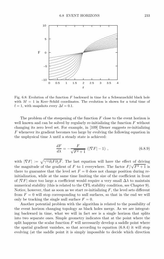
6.8 EVENT HORIZONS 233
–10
–5
0
5
10
0 0.5 1 1.5 2 2.5 3 3.5 4
r
F
Fig. 6.8: Evolution of the function F backward in time for a Schwarzschild black holewith M = 1 in Kerr–Schild coordinates. The evolution is shown for a total time oft = 1, with snapshots every ∆t = 0.1.
The problem of the steepening of the function F close to the event horizon iswell known and can be solved by regularly re-initializing the function F withoutchanging its zero level set. For example, in [109] Diener suggests re-initializingF whenever its gradient becomes too large by evolving the following equation inthe unphysical time λ until a steady state is achieved:
dF
dλ= − F√
F 2 + 1(|∇F | − 1) , (6.8.9)
with |∇F | :=√
γij∂iF∂jF . The last equation will have the effect of drivingthe magnitude of the gradient of F to 1 everywhere. The factor F/
√F 2 + 1 is
there to guarantee that the level set F = 0 does not change position during re-initialization, while at the same time limiting the size of the coefficient in frontof |∇F | since too large a coefficient would require a very small ∆λ to maintainnumerical stability (this is related to the CFL stability condition, see Chapter 9).Notice, however, that as soon as we start re-initializing F , the level sets differentfrom F = 0 will stop corresponding to null surfaces, so that in the end we willonly be tracking the single null surface F = 0.
Another potential problem with the algorithm is related to the possibility ofthe event horizon changing topology as black holes merge. As we are integrat-ing backward in time, what we will in fact see is a single horizon that splitsinto two separate ones. Simple geometry indicates that at the point where thesplit happens the scalar function F will necessarily develop a saddle point wherethe spatial gradient vanishes, so that according to equation (6.8.4) it will stopevolving (at the saddle point it is simply impossible to decide which direction

234 EVOLVING BLACK HOLE SPACETIMES
is “outward”). Luckily, this seems to be one of those situations where the in-accuracies of numerical approximations come to our help: Numerically, we willnever be exactly on the saddle point of F , so that the gradient will never vanishcompletely. Empirically we find that the surface simply evolves right through atopology change without any problem.
The discussion presented here has been very brief. For a much more detailedexplanation of the null surface algorithm the reader should look at the recent pa-per by Diener on a general-purpose three-dimensional event horizon finder [109].
6.9 Isolated and dynamical horizons
As we have already mentioned, the formal definition of a black hole is basedon the notion of an event horizon, which marks the boundary between thoselight rays that escape to infinity and those that do not. The global nature ofthis definition, however, means that it can not be used to characterize a blackhole locally during an evolution. Recently, however, a new theoretical paradigmhas emerged to describe black holes locally, based on the notions of isolated anddynamical horizons.70 These notions allow us, for example, to define the mass andangular momentum associated with a black hole during a dynamical evolution,and have rapidly been adopted in numerical relativity simulations [113, 181].The theory behind these new concepts is still being actively developed, and weare now at the point where numerical relativity is inspiring, and perhaps evendriving, further theoretical developments.
There is already an extensive literature devoted to isolated and dynamicalhorizons [32, 33, 34, 38, 35, 36, 39, 148, 149]. Here we will just consider some ofthe basic notions and their application to numerical relativity. We will start byrecalling the definition of a trapped surface: A closed two-dimensional surface Sis said to be an outer trapped surface if the expansion of the outgoing null vectorsnormal to S is everywhere negative. In the special case when this expansion iszero the surface is called marginally trapped. An apparent horizon is then definedas the outermost marginally trapped surface.
We can prove that provided the weak energy condition holds (and in par-ticular it does in vacuum), then the existence of a trapped surface implies theformation of a singularity. This means, in particular, that if cosmic censorshipis true then a trapped surface implies the existence of an event horizon, i.e. ablack hole (see e.g. [161]).
We now define a non-expanding horizon as a null three-dimensional hyper-surface H , with topology S2×, that is foliated by marginally trapped surfaces(see Figure 6.9). Notice that if we have a stationary black hole, then necessarilythe world-tube formed by simply stacking the apparent horizons at each spatialhypersurface will form a non-expanding horizon.
70One might argue that black holes are by definition non-local. However, the new conceptsapply to geometric objects that are more closely related to the astrophysical notion of a blackhole: something that forms as a result of gravitational collapse and has a horizon around it.
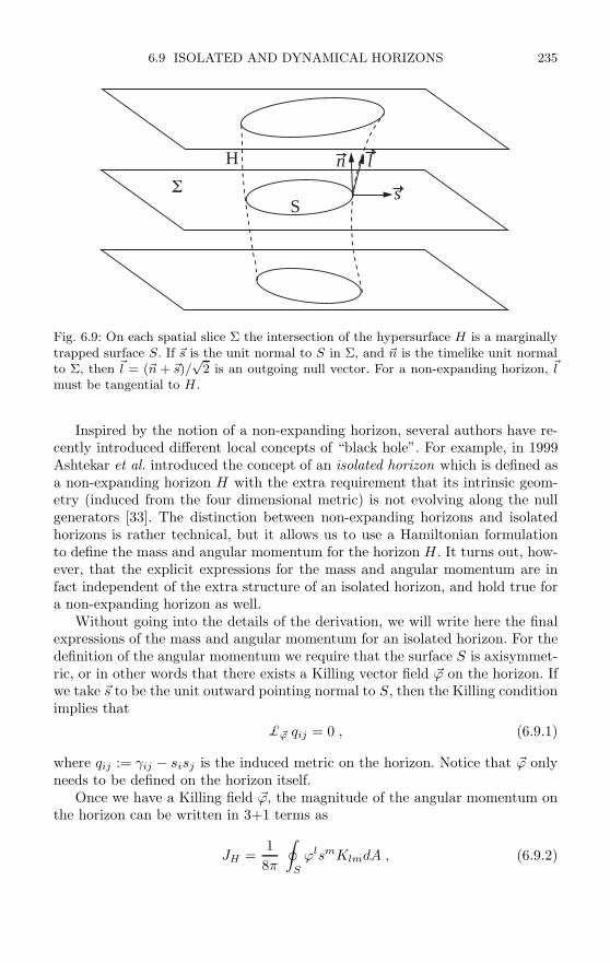
6.9 ISOLATED AND DYNAMICAL HORIZONS 235
Ss
n lH
Fig. 6.9: On each spatial slice Σ the intersection of the hypersurface H is a marginallytrapped surface S. If s is the unit normal to S in Σ, and n is the timelike unit normalto Σ, then l = (n + s)/
√2 is an outgoing null vector. For a non-expanding horizon, l
must be tangential to H .
Inspired by the notion of a non-expanding horizon, several authors have re-cently introduced different local concepts of “black hole”. For example, in 1999Ashtekar et al. introduced the concept of an isolated horizon which is defined asa non-expanding horizon H with the extra requirement that its intrinsic geom-etry (induced from the four dimensional metric) is not evolving along the nullgenerators [33]. The distinction between non-expanding horizons and isolatedhorizons is rather technical, but it allows us to use a Hamiltonian formulationto define the mass and angular momentum for the horizon H . It turns out, how-ever, that the explicit expressions for the mass and angular momentum are infact independent of the extra structure of an isolated horizon, and hold true fora non-expanding horizon as well.
Without going into the details of the derivation, we will write here the finalexpressions of the mass and angular momentum for an isolated horizon. For thedefinition of the angular momentum we require that the surface S is axisymmet-ric, or in other words that there exists a Killing vector field ϕ on the horizon. Ifwe take s to be the unit outward pointing normal to S, then the Killing conditionimplies that
£ϕ qij = 0 , (6.9.1)
where qij := γij − sisj is the induced metric on the horizon. Notice that ϕ onlyneeds to be defined on the horizon itself.
Once we have a Killing field ϕ, the magnitude of the angular momentum onthe horizon can be written in 3+1 terms as
JH =18π
∮S
ϕlsmKlmdA , (6.9.2)
236 EVOLVING BLACK HOLE SPACETIMES
with Kij the extrinsic curvature of the tri-dimensional spatial hypersurfaces Σand dA the area element on S. It is instructive to compare the expression forJH above with the expression for the ADM angular momentum discussed inAppendix A, equation (A.8). Both expressions are essentially identical with theexception that one is calculated at the horizon and the other at infinity. TheKilling field ϕ is needed in equation (6.9.2) in order to identify the correct angularcoordinate around the horizon. In [113], Dreyer at al. describe an algorithm forfinding an approximate Killing field ϕ on a closed surface S (which may or maynot be an apparent horizon). This algorithm is now being used by a large numberof groups doing numerical simulations of black holes spacetimes.
Having found the angular momentum, the horizon mass MH turns out to begiven by
M2H =
AH
16π+
4πJ2HAH
, (6.9.3)
with AH the area of the surface S. This is nothing more than the standardrelation for a rotating black hole, equation (1.16.10). Notice, however, that thisis not just a definition, but the result of the Hamiltonian approach.
The definition of isolated horizons, though extremely useful, has neverthelessthe drawback that it only applies to black holes that are stationary. Becauseof this, theoretical work has now shifted to the study of the so-called dynam-ical horizons. In 1994 Hayward introduced the notion of a future outer trap-ping horizon, which is essentially a three-dimensional hypersurface foliated bymarginally trapped surfaces [162]. This definition, though very similar to that ofa non-expanding horizon, is nevertheless more general as it does not ask for thehypersurface to be null. Notice that in a dynamical situation we in fact expectthe world-tube formed by the apparent horizons to be spacelike. This last state-ment can in fact be proven formally, but for our purposes it is enough to noticethat if a black hole is dynamical, the area of the apparent horizon must grow(this is the so-called second law of black hole dynamics, see e.g. [160]), whilethe area of a null surface that momentarily coincides with the apparent horizonremains constant by definition (the expansion is zero). The apparent horizonmust therefore move outwards faster than light, i.e. the world-tube of apparenthorizons is spacelike. This result motivates the definition of a dynamical horizonas a spacelike three-dimensional hypersurface H with topology S2 × that isfoliated by marginally trapped surfaces [37]. Notice that this definition is almostthe same as that of a non-expanding horizon given above, with the importantdifference that now the hypersurface is not null, but is instead spacelike.
We can use the notion of a dynamical horizon to define fluxes and balancelaws for mass and angular momentum on a horizon, and we can also define theangular momentum of the dynamical horizon itself [37, 72, 148]. In this case westill need to find a “rotation” vector ϕ which, however, does not need to be aKilling field anymore. It is enough now for the vector ϕ to be such that it hasclosed orbits on the horizon and zero divergence. This definition, unfortunately,

6.9 ISOLATED AND DYNAMICAL HORIZONS 237
is somewhat ambiguous since in general we can have many different vector fieldson the horizon that satisfy these conditions, and each will give us a differentvalue for the angular momentum.
As a final comment, it should be mentioned that the need to study the evo-lution of the direction as well as the magnitude of the angular momentum of ablack hole during a dynamical simulation has recently led to the introduction ofthe so-called coordinate angular momenta, for which we simply take the standardEuclidean rotational vector fields around the coordinate axis, ϕx = (0,−z, y),ϕy = (z, 0,−x) and ϕz = (−y, x, 0), to define the three components of the angu-lar momentum of the horizon [94]. These coordinate angular momenta are notwell defined in any formal way, the main problem being that it is difficult toassociate a “vector” with the horizon, because, in differential geometry vectorsare only defined at points, and a single vector cannot be related clearly with asurface. Still, we would like to be able to recover the notion from classical me-chanics that requires three numbers to completely define the angular momentumof a physical object. Keeping this in mind, the informal definition of coordinateangular momenta has already been found to provide useful physical informationduring the simulation of black hole collisions. We are now in a situation wherecurrent numerical simulations are demanding further theoretical developments.These are indeed exciting times.
7
RELATIVISTIC HYDRODYNAMICS
7.1 Introduction
In the previous Chapter we considered the simulation of black hole spacetimes,which corresponds to the study of the Einstein field equations in their purestform, i.e. in vacuum. It is clear, however, that most relativistic astrophysicalsystems involve matter sources: stars, accretion flows, jets, gravitational col-lapse, etc. Since many of these systems involve gases it is natural to model themusing the theory of fluid dynamics. The fluid approximation describes matter asa continuum, this means that when we consider an “infinitesimal” fluid elementwe are in effect assuming that the fluid element is small compared to the systemas a whole, but still big enough to contain a very large number of particles. Inorder for the fluid model to be a good approximation there are two basic condi-tions that must be satisfied: Both the mean distance between the particles andthe mean free path between collisions must be much smaller than the macro-scopic characteristic length of the system. Fluids are therefore particularly badat modeling collisionless particles, unless their paths are not expected to cross,in which case we can use a fluid with zero pressure (known as “dust”).
The state of the fluid is usually described in terms of the velocity field of thefluid elements vi, the mass-energy density ρ, and the pressure p. There are twodistinct approaches that can be used to follow the fluid motion. One possibility isto consider a fixed coordinate system and study the motion of the fluid as seen byobservers at rest in this coordinate system – such an approach is called Eulerian(as in the Eulerian observers of the 3+1 formulation). The other possibility is totie the coordinate system to the fluid elements themselves, corresponding to theso-called Lagrangian approach. The Lagrangian point of view has some advan-tages in the case of simple fluid motion (e.g. spherical collapse), as conservationof mass can be trivially guaranteed. However, a Lagrangian scheme becomes in-adequate when the fluid motion has large shears since in that case the coordinatesystem can easily become entangled. Because of this, in the presentation givenhere we will always consider a Eulerian approach.
In the following Sections we will derive the dynamical equations governingthe motion of a perfect fluid, known as the Euler equations, both in the specialand general relativistic cases, and will also consider some simple equations ofstate. We will later discuss the hyperbolicity properties of the hydrodynamicsystem of evolution equations, and consider the concept of weak solutions andshock waves. Finally, we will discuss how to generalize the Euler equations to thecase of imperfect fluids with heat conduction and viscosity. The description pre-
238

7.2 SPECIAL RELATIVISTIC HYDRODYNAMICS 239
sented here will be very brief. There exists, however, a large literature dedicatedexclusively to the study of fluid mechanics, most notably the beautiful book ofLandau and Lifshitz [184]. There are also many books that discuss the numeri-cal treatment of the hydrodynamic equations, particularly in the non-relativisticcase. In the case of relativity there is the recent book by Wilson and Mathewson relativistic numerical hydrodynamics [300], and the review papers by Martiand Muller [200], and Font [129].
7.2 Special relativistic hydrodynamics
The starting point to the study of relativistic hydrodynamics is the stress-energytensor for a perfect fluid, i.e. a fluid with zero viscocity and no heat conduction.Such a stress-energy tensor has already been introduced in equation (1.12.4) ofChapter 1, and has the form
Tµν = (ρ + p)uµuν + p ηµν , (7.2.1)
where uµ is the 4-velocity of the fluid elements (the average 4-velocity of theparticles), ρ and p are the energy density and pressure as measured in the fluid’srest frame, and where, for the moment, we have assumed that we are in specialrelativity so the metric is given by the Minkowski tensor gµν = ηµν .
The stress-energy tensor above is usually written in a simplified form by firstseparating the total energy density ρ into contributions coming from the restmass energy density ρ0 and the internal energy:
ρ = ρ0 (1 + ε) , (7.2.2)
where ε is the specific internal energy (internal energy per unit mass) of the fluid.Let us now introduce the so-called specific enthalpy of the fluid defined as71
h := 1 + ε +p
ρ0. (7.2.3)
In terms of h, the stress-energy tensor then takes the simple form
Tµν = ρ0h uµuν + p ηµν . (7.2.4)
The rest mass energy density is also often written in terms of the particlenumber density n as
ρ0 = nm , (7.2.5)
with m the rest mass of the fluid particles.
71In thermodynamics the enthalpy H is defined as the sum of the internal energy U plusthe pressure times the volume, H = U + pV . In other words, the enthalpy represents the totalenergy in the system capable of doing mechanical work. In relativity we also add the rest massenergy M to the definition of enthalpy, so that H = M +U +pV = M(1+ ε)+pV . The specificenthalpy is then defined as the enthalpy per unit mass: h = H/M = 1 + ε + p/ρ0.
240 RELATIVISTIC HYDRODYNAMICS
A note about the interpretation of the fluid variables is important at thispoint. In the case of general relativity, the 3+1 evolution equations and theHamiltonian constraint involve the energy density of matter as a source of thegravitational field. However, this energy density is assumed to be measured in theEulerian reference frame (the one associated with the observers whose 4-velocityis normal to the spatial hypersurface), which will in general differ from the fluid’sframe of reference (the Lagrangian frame). In order to avoid confusion we willfrom now on denote the energy density that appears in the ADM equations byρADM. We can derive the relationship between the different energy densities bystarting from the definition of ρADM:
ρADM := nµnνTµν , (7.2.6)
with nµ the unit normal to the spacelike hypersurfaces. Substituting the abovestress-energy tensor here and using the fact that nµnµ = −1 we find
ρADM = ρ0h (uµnµ)2 − p = ρ0hW 2 − p , (7.2.7)
where we have definedW := −uµnµ = u0 . (7.2.8)
The last equality follows from the fact that, in special relativity, we havenµ = (−1, 0). Finally, using the fact that uµuµ = −1 we obtain
W =
(1 +
∑i
ui
)1/2. (7.2.9)
But this is nothing more than the Lorentz factor 1/√
1 − v2, since the standardthree-dimensional speed of the fluid is given by
vi = ui/u0 =(1 − v2
)1/2ui , (7.2.10)
which can be shown to imply
W = 1/√
1 − v2 . (7.2.11)
In the particular case when the local coordinates follow the fluid element wehave W = 1, and the energy densities become equal:
ρADM = ρ0hW 2 − p = ρ0h − p = ρ0(1 + ε) = ρ . (7.2.12)
Notice, however, that if the flow is non-uniform we can not adapt the coordinatesystem to follow the fluid elements (the Lagrangian approach) without beingforced to replace the Minkowski metric ηµν with a more general metric gαβ ,since the fluid motion will in general deform the volume elements.
7.2 SPECIAL RELATIVISTIC HYDRODYNAMICS 241
The state of the fluid at any given time is given in terms of the six variables(ρ0, ε, p, vi), which from now on will be called the primitive variables. The evo-lution equations for the fluid now follow from the conservation laws. We have infact two sets of conservation laws, namely the conservation of particles and theconservation of energy-momentum:
∂µ (ρ0uµ) = 0 , (7.2.13)∂µT µν = 0 . (7.2.14)
Notice that these conservation laws provide us with five equations. In order toclose the system we therefore need an equation of state which can be assumedto be of the form
p = p (ρ0, ε) . (7.2.15)
To proceed let us now introduce the quantity
D := ρ0W , (7.2.16)
which is nothing more than the rest mass density as seen in the Eulerian frame.The conservation of particles now implies
∂tD + ∂k
(Dvk
)= 0 . (7.2.17)
This is known as the continuity equation and has exactly the same form as in theNewtonian case, but now D includes the relativistic correction coming from theLorentz factor W . The continuity equation can be interpreted as an evolutionequation for D.
For the conservation of momentum we first define the quantities
Sµ := ρ0hWuµ . (7.2.18)
Notice that since ui = Wvi, the spatial components Si = ρ0hW 2vi are nothingmore that the momentum density as seen in the Eulerian frame, with the correctLorentz factors (the fact that the enthalpy h appears in the expression for Si
shows that in relativity the pressure contributes to the momentum density). Interms of Sµ, the mixed components of the stress-energy tensor become
T µν =
Sνuµ
W+ p δµ
ν , (7.2.19)
The conservation of momentum then takes the form
∂µ (Siuµ/W + p δµ
i ) = 0⇒ ∂tSi + ∂k
(Siv
k)
+ ∂ip = 0 . (7.2.20)
These are the evolution equations for the momentum density and are knownas the Euler equations. Notice that they have a structure similar to that of the
242 RELATIVISTIC HYDRODYNAMICS
continuity equation, but now there is an extra term given by the gradient of thepressure. The momentum density can then change both because of the flow ofmomentum out of the volume element represented by the term ∂j
(Siv
j), and
because of the existence of a force given by the gradient of the pressure ∂ip. TheEuler equations above have again exactly the same form as in the Newtoniancase, but now the definition of the momentum density Si includes the relativisticcorrections.
We are still missing an evolution equation for the energy density. Such anequation can be obtained in a number of different ways. Experience has shownthat it is in fact convenient to subtract the rest mass energy density in orderto have higher accuracy, since for systems that are not too relativistic the restmass can dominate the total energy density. However, there are several non-equivalent ways to do this. As a first approach, consider the internal energydensity as measured in the Eulerian frame:
E = ρ0εW . (7.2.21)
Notice that there is only one Lorentz factor W coming from the Lorentz contrac-tion of the volume elements, since the specific internal energy ε can be considereda scalar (this is by definition the internal energy per particle in the fluid’s frame).In order to derive an evolution equation for E we first notice that the conserva-tion equations imply that
∂µ (uνT µν) = T µν∂µuν . (7.2.22)
Substituting here the expression for the stress-energy tensor, and rememberingthat uµuµ = −1 implies uµ∂νuµ = 0, we find
∂µ (uνT µν) = p ∂µuµ . (7.2.23)
On the other handuνT µν = −ρ0 (1 + ε)uµ , (7.2.24)
and using now the conservation of particles, this implies
∂µ (uνT µν) = −∂µ (ρ0εuµ) . (7.2.25)
Collecting results we obtain
∂µ (ρ0εuµ) + p ∂µuµ = 0 , (7.2.26)
which can be rewritten as
∂tE + ∂k
(Evk
)+ p
[∂tW + ∂k
(Wvk
)]= 0 . (7.2.27)
This equation has been used successfully by Wilson and collaborators to evolverelativistic fluids (see e.g. [300]). However, as an evolution equation for E it has
7.2 SPECIAL RELATIVISTIC HYDRODYNAMICS 243
one serious drawback, namely that it also involves the time derivative of W ,so that it can not be written as a balance law, which in particular makes itimpossible to use for analyzing the characteristic structure of the system.
Fortunately, there exists an alternative way of subtracting the rest mass en-ergy from the system that does yield an equation in balance law form. We cansimply decide to evolve instead the difference between the total energy densityand the mass energy density as measured in the Eulerian frame:
E := ρADM − ρ0W = ρADM − D = ρ0hW 2 − p − D . (7.2.28)
Notice that the energies E and E differ since E does not include contributionsfrom the kinetic energy while E does. To find the evolution equation for E we firstnotice that from the definition of Sµ we have S0 = ρ0hW 2. The conservation ofenergy then takes the form
0 = ∂µT 0µ = ∂µ
(S0uµ/W + pη0µ
), (7.2.29)
which immediately yields
∂tS0 + ∂k
(S0vk
)− ∂tp = 0 . (7.2.30)
Using now the evolution equation for D we finally find
∂tE + ∂k
[(E + p) vk
]= 0 , (7.2.31)
where we used the fact that S0 = E + D + p.Our set of evolution equations then becomes a system of conservation laws
of the form72
∂tD + ∂k
(Dvk
)= 0 , (7.2.32)
∂tSi + ∂k
(Siv
k + p δki
)= 0 , (7.2.33)
∂tE + ∂k
[(E + p) vk
]= 0 , (7.2.34)
with the conserved quantities (D, Si, E) given in terms of the primitive quantities(ρ0, ε, p, vi) as
D = ρ0W , Si = ρ0hW 2vi , E = ρ0hW 2 − p − ρ0W . (7.2.35)
Note that the Euler equations are frequently written for the speed vi insteadof the flux Si and have the form (see e.g. [297])
∂tvi + vk∂kvi = − [∂ip + vi∂tp] /(ρ0hW 2) . (7.2.36)
These equations can be easily derived by combining the evolution equations forD, Si and E . However, they are not as convenient as the evolution equations for
72The hydrodynamic equations in the conservative form given here were first derived byMarti, Ibanez, and Miralles at the University of Valencia in Spain and are often called theValencia formulation of relativistic hydrodynamics [130, 198] (see also [129, 200]).
244 RELATIVISTIC HYDRODYNAMICS
Si since they are not written as conservation laws, and in particular involve thetime derivative of the pressure.
There is another important consequence of the conservation equations. Con-sider the contraction
uµ∂νT µν = 0 . (7.2.37)
Substituting the expression for T µν, and using again the fact that uµ∂νuµ = 0,we find
uµ∂µp − ∂ν (ρ0huµ) = 0 . (7.2.38)
This can be further simplified with the help of the equation for conservation ofparticles to
uµ∂µp − ρ0uµ∂µh = 0 , (7.2.39)
and using now the expression for the specific enthalpy h we finally obtain
dε
dτ+ p
d
dτ
(1ρ0
)= 0 , (7.2.40)
where d/dτ := uµ∂µ is the derivative along the trajectory of the fluid elements.This equation is in fact nothing more than the local version of the first law ofthermodynamics. To see this, consider a fluid element with rest mass M , internalenergy U , and volume V . We then have in general that
ρ0 =M
V⇒ dV = Md
(1ρ0
), (7.2.41)
and similarly
ε =U
M⇒ dU = Mdε . (7.2.42)
The first law of thermodynamics then implies that
dQ = dU + pdV = M
[dε + p d
(1ρ0
)]. (7.2.43)
This shows that (7.2.40) is precisely the first law of thermodynamics for a fluidelement for which dQ = 0 (this is to be expected since by definition a perfectfluid has no heat conduction). And since in general dQ = TdS, with T thetemperature and S the entropy of the fluid, we see that a perfect fluid behavesin such a way that entropy is preserved along flow lines.
Let us now go back and consider the relation between the primitive and con-served variables (7.2.35). In the Newtonian limit these relations reduce to D = ρ0,Si = ρ0vi and E = ρ0(ε + v2/2), so that they are very easy to invert. In the rela-tivistic case, however, inverting the relations becomes much more difficult sincefirst W involves v2, and also the pressure appears explicitly in the expression for
7.3 GENERAL RELATIVISTIC HYDRODYNAMICS 245
E , so the equation of state is needed in order to recover the primitive variables.Unfortunately, the evolution equations for the conserved quantities involve theprimitive variables directly, so that these must be recovered every time step. Thisrequires that an algorithm for recovering such variables is implemented. Such analgorithm starts by choosing some trial value of the pressure p∗ (for example theold value at the corresponding grid cell). Then, from the expressions for D andE we can recover the speed vi in the following way
vi(p∗) =Si
ρ0hW 2=
Si
E + D + p∗. (7.2.44)
Having found vi we then compute W as
W (p∗) =1√
1 − v2(p∗). (7.2.45)
This allows us to find the density ρ0 as
ρ0(p∗) =D
W (p∗). (7.2.46)
Finally, we find the specific internal energy ε through the definition of h
ε(p∗) =E + ρ0W (1 − W ) + p∗
(1 − W 2
)ρ0W 2
=E + D (1 − W (p∗)) + p∗
(1 − W 2(p∗)
)DW (p∗)
(7.2.47)
Of course, the chosen value of p∗ will almost certainly not satisfy the equationof state p = p(ρ0, ε), so we must now evaluate the residual r(p∗) defined as
r(p∗) := p(ρ0(p∗), ε(p∗)) − p∗ , (7.2.48)
and change the value of p∗ until this residual vanishes. This can typically be ac-complished by standard non-linear root-finding techniques (e.g. one-dimensionalNewton–Raphson). For some simple equations of state, such as that of an idealgas discussed in Section 7.5, the whole procedure can in fact be done analyticallyand involves finding the physically admissible root of a high order polynomial (afourth order polynomial in the case of an ideal gas). However, this is typicallymore computationally expensive than using the non-linear root finder directly.
7.3 General relativistic hydrodynamics
The generalization of the evolution equations (7.2.32)–(7.2.34) to the case of anon-trivial gravitational field is rather straightforward. We again start from thestress-energy tensor for a perfect fluid, but now for an arbitrary metric gµν :
Tµν = ρ0huµuν + p gµν , (7.3.1)
246 RELATIVISTIC HYDRODYNAMICS
where as before uµ is the 4-velocity of the fluid elements, ρ0 is the rest massenergy density measured in the fluid’s rest frame, p is the pressure and h is thespecific enthalpy
h := 1 + ε +p
ρ0, (7.3.2)
with ε the specific internal energy. The evolution equations for the fluid againfollow from the conservation laws, which however now take the form
∇µ (ρ0uµ) = 0 , (7.3.3)∇µT µν = 0 . (7.3.4)
Using the fact that the divergence of a vector can be written in general as
∇µξµ =1√−g
∂µ
(√−g ξµ)
, (7.3.5)
with g the determinant of the metric tensor gµν , we can immediately rewrite theconservation of particles as
∂µ
(√−g ρ0uµ)
= 0 , (7.3.6)
and the conservation of energy and momentum as
∂µ
(√−g T µν
)=
√−g ΓαµνT µ
α , (7.3.7)
with Γαµν the Christoffel symbols associated with the metric gµν .
We now assume that we are using a standard 3+1 decomposition of spacetime,in which case we find
g = −α2γ ⇒ √−g = α√
γ , (7.3.8)
with α the lapse function and γ the determinant of the spatial metric γij .Just as we did in special relativity, let us define the scalar parameter W as
W := −uµnµ , (7.3.9)
with nµ the unit normal to the spatial hypersurfaces. In this case we havenµ = (−α, 0), so that
W = αu0 . (7.3.10)
Define now
vi :=ui
αu0+
βi
α, (7.3.11)
with βi the shift vector. With this definition vi is precisely the speed of the fluidelements as seen by the Eulerian observers. To see this notice that ui/u0 is thecoordinate speed of the fluid elements, so we first need to add the shift to go tothe Eulerian reference frame and then divide by the lapse to use the proper time

7.3 GENERAL RELATIVISTIC HYDRODYNAMICS 247
of the Eulerian observers instead of coordinate time. Notice also that since uµ isa 4-vector while vi is only a 3-vector, when we lower the indices we have
ui = giµuµ = βiu0 + γikuk
= βiu0 + γiku0
(αvk − βk
)= αu0vi = Wvi . (7.3.12)
Using again the fact that uµuµ = −1, we find that W takes the simple form
W = 1/√
1 − v2 , (7.3.13)
where now v2 := γijvivj , i.e. W is again the Lorentz factor as seen by the
Eulerian observers. Define again D as the rest mass density measured by theEulerian observers
D := ρ0W , (7.3.14)
we can then rewrite the conservation of particles as
∂t (√
γ D) + ∂k
[√γ D
(αvk − βk
)]= 0 . (7.3.15)
This is again a conservation law for D, but in contrast to the case of specialrelativity it involves the lapse α, the shift vector βk, and the determinant of thespatial metric γ (compare with equation (7.2.32)).
For the conservation of momentum we again introduce the quantities
Sµ := ρ0hWuµ , (7.3.16)
and rewrite the stress-energy tensor as
T µν =
uµSν
W+ p δµ
ν . (7.3.17)
The conservation of momentum then becomes
∂t (√
γSi) + ∂k
√γ[Si
(αvk − βk
)+ αp δk
i
]= α
√γ Γµ
νiTνµ , (7.3.18)
where Si = ρ0hWui = ρ0hW 2vi. The last equations are the general relativisticversion of the Euler equations. When we compare them with their special rela-tivistic version (7.2.33) we see that in the case of general relativity, apart fromthe lapse and shift factors that correct for the motion of the Eulerian observers,we don’t have strict conservation of momentum anymore since there is a sourceterm on the right hand side that represents the gravitational forces.
Finally, for the conservation of energy we again start by defining
E = ρ0hW 2 − p − D . (7.3.19)
The conservation of energy then takes the form
∂µ
(α√
γ T 0µ)
= −α√
γ Γ0µνT µν . (7.3.20)
248 RELATIVISTIC HYDRODYNAMICS
It is in fact convenient to rewrite the term on the left hand side as
∂µ
(α√
γ T 0µ)
=1α
∂µ
(α2
√γ T 0µ
)−√γ T 0µ∂µα , (7.3.21)
so that the conservation of energy becomes
∂µ
(α2
√γ T 0µ
)= α2
√γ(T 0µ∂µ ln α − Γ0µνT µν
). (7.3.22)
Using now the expression for T 0µ we obtain, after some algebra,
∂µ
(α2
√γ T 0µ
)= ∂t
[√γ(ρ0hW 2 − p
)]+ ∂k
√γ[ρ0hW 2
(αvk − βk
)+ pβk
], (7.3.23)
and using the evolution equation for D we find that the final expression for theconservation of energy takes the form
∂t (√
γ E) + ∂k
√γ[E (αvk − βk
)+ αpvk
]= α2
√γ(T 0µ∂µ lnα − Γ0µνT µν
).
The final set of evolution equations is then
∂t (√
γ D) + ∂k
[√γ D
(αvk − βk
)]= 0 , (7.3.24)
∂t (√
γ Si) + ∂k
√γ[Si
(αvk − βk
)+ αpδk
i
]= α
√γ Γµ
νiTνµ , (7.3.25)
∂t (√
γ E) + ∂k
√γ[E (αvk − βk
)+ αpvk
]= α2
√γ(T 0µ∂µ lnα
− Γ0µνT µν)
, (7.3.26)
where the conserved quantities (D, Si, E) and primitive variables (ρ0, ε, p, vi) arerelated through
D = ρ0W , Si = ρ0hW 2vi , E = ρ0hW 2 − p − D . (7.3.27)
Notice that the system of equations (7.3.24)–(7.3.26) reduces to the special rel-ativistic counterpart (7.2.32)-(7.2.34) when we take α = 1, βi = 0 and γij = δij ,in which case Γα
µν = 0 and the system is truly conservative. The presence of anon-trivial gravitational field implies that there is no longer true conservation ofenergy and momentum, but the equations are still in the form of balance laws:∂tu + ∂kF k(u) = s(u).
Before concluding this Section, it is important to write down the relationbetween the quantities (D, Si, E) and the matter terms measured by the Eulerianobservers that appear in the ADM equations, namely the energy density ρADM,the momentum density ji
ADM and the stress tensor SijADM. Using the expression
for T µν we find
ρADM := nµnνTµµ = ρ0hW 2 − p = E + D , (7.3.28)jiADM := −nµP νiTµν = ρ0hW 2vi = Si , (7.3.29)
SijADM := PµiP νjTµν = ρ0hW 2vivj + γijp , (7.3.30)
where P µν = gµν + nµnν is the standard projection operator onto the spatialhypersurfaces.

7.4 3+1 FORM OF THE HYDRODYNAMIC EQUATIONS 249
7.4 3+1 form of the hydrodynamic equations
The general relativistic hydrodynamic evolution equations (7.3.24)–(7.3.26) de-rived in the previous Section have been written as a set of balance laws, whichhas some advantages from a numerical point of view. However, from the per-spective of the 3+1 formulation of general relativity they are not written in themost convenient form as they are not manifestly 3-covariant. In this Section wewill rewrite these equations as tensor equations in 3+1 language.
Let us start from the evolution equation for the rest mass density D. Sincethis is just the particle density as seen by the Eulerian observers, times the restmass of the individual particles, it is in fact a scalar in 3+1 terms. The originalevolution equation has the form
∂t (√
γ D) + ∂k
[√γ D
(αvk − βk
)]= 0 . (7.4.1)
Notice first that, for any three-dimensional vector wi we have
1√γ
∂k
(√γwk
)= Dkwk , (7.4.2)
with Dk the covariant derivative associated with the spatial metric γij . Thisimplies that
1√γ
∂k
[√γ D
(αvk − βk
)]= Dk
(αDvk
)− (Dkβk)D − βk∂kD . (7.4.3)
On the other hand
1√γ
∂t (√
γ D) = ∂tD +D
2∂t ln γ . (7.4.4)
Now, from the ADM evolution equations for the spatial metric (2.3.12), we caneasily find that
∂t ln γ = −2αK + 2Dkβk , (7.4.5)
with K the trace of the extrinsic curvature Kij . Collecting results we find thatthe evolution equation for D in 3+1 language takes the final form
∂tD − βk∂kD + Dk
(αDvk
)= αKD . (7.4.6)
This equation is clearly a scalar equation. The different terms are easy to inter-pret: The shift appears only in the advection term, as it should, since the onlyrole of the shift is to move the coordinate lines. The last term on the left handside shows that the change in D along the normal lines is given essentially by thedivergence of the flux of particles. Finally, the source term shows that the densityof particles D can also change because of an overall change in the spatial volumeelements. For example, in the case of cosmology the so-called cosmological fluidis co-moving with the Eulerian observers so that vi = βi = 0, but the density of

250 RELATIVISTIC HYDRODYNAMICS
particles still becomes smaller with time because of the overall expansion of theUniverse (K < 0).
It is also interesting to note that in the last equation the shift appears asan advection term that is not in flux-conservative form (the shift is outside thespatial derivatives). The flux conservative form (7.3.24) comes about because aswe bring the shift vector into the spatial derivative we pick up a term with thedivergence of the shift. This term is canceled by a corresponding term comingfrom the time derivative of the volume element. This shows that, quite generally,advection terms on the shift can be transformed into flux conservative type termsby bringing a
√γ factor into the time derivative.
Consider next the evolution equation for E . Again, since this is by definitionthe energy density measured by the Eulerian observers minus the rest massdensity, E = ρADM − D = ρ0hW 2 − p − D, it is clearly a scalar quantity in 3+1terms. Its original evolution equation is
∂t (√
γ E) + ∂k
√γ[E (αvk − βk
)+ αpvk
]= α2
√γ(T 0µ∂µ lnα − Γ0µνT µν
).
Let us first look at the source term. Using the expression for the stress-energy ten-sor (7.3.1), the definition of vi (7.3.11), and the expressions for the 4-Christoffelsymbols in 3+1 language found in Appendix B, it is not difficult to show that
α2(T 0µ∂µ lnα − Γ0µνT µν
)= ρ0hW 2 (αvmvnKmn − vm∂mα) + αpK
= (E + p + D) (αvmvnKmn − vm∂mα) + αpK . (7.4.7)
We can now rewrite the left hand side of the evolution equation for E in ex-actly the same way as the evolution equation for D. We then find the followingevolution equation for E in 3+1 form
∂tE − βk∂kE + Dk
[αvk (E + p)
]= (E + p + D) (αvmvnKmn − vm∂mα)+ αK (E + p) . (7.4.8)
The last term on the right hand side is interesting. Assume that we have a fluidthat is co-moving with the Eulerian observers so that vk = βk = 0, we then findthat ∂tE = αK(E +p). This shows that the internal energy density changes bothas a reflection of a simple change in the volume elements (αKE), and because ofthe existence of a non-zero pressure (αpK). But we know that αK = −∂t ln
√γ,
so that αpK = −p ∂t ln√
γ, which is nothing more than the work done by thefluid as space expands. That is, the term αpK in the source term is there inaccordance with the first law of thermodynamics.
Finally, let us consider the evolution equation for the momentum density Si.Since we have Si = ρ0hW 2vi, then we can consider Si a vector with respect tothe 3-geometry. Its original evolution equation is
∂t (√
γSi) + ∂k
√γ[Si
(αvk − βk
)+ αp δk
i
]= α
√γ Γµ
νiTνµ , (7.4.9)
7.4 3+1 FORM OF THE HYDRODYNAMIC EQUATIONS 251
From the expression for the stress-energy tensor, the right hand side of thisequation can easily be shown to be
α√
γ ΓµνiT
νµ = p ∂i (α
√γ) + α
√γ
ρ0h
2uµuν∂igµν . (7.4.10)
Substituting now the components of the 4-metric gµν in terms of 3+1 quantitieswe find, after some algebra, that
α
2uµuν∂igµν = W 2
[−∂iα + vkDiβk + (3)Γm
ik
ukvm
u0
], (7.4.11)
where (3)Γmik are the Christoffel symbols associated with the 3-geometry. On the
other hand we have1√γ
∂t (√
γSi) = ∂tSi − αKSi + SiDkβk , (7.4.12)
and1√γ
∂k
[√γSi
(αvk − βk
)]= Dk
[αSi
(vk − βk
)]+ Sm (αvn − βn) (3)Γm
in . (7.4.13)
Collecting results we find that the evolution equation for Si becomes
∂tSi − αKSi + Dk
(αSiv
k)− βkDkSi + Sm
(αvk − βk
)(3)Γm
ik +1√γ
∂i (α√
γ p)
=p√γ
∂i (α√
γ) + ρ0hW 2
[−∂iα + vkDiβk + (3)Γm
ik
ukvm
u0
], (7.4.14)
which can be simplified to
∂tSi − £βSi + Dk
(αSiv
k)
+ ∂i (αp) = − (E + D) ∂iα + αKSi . (7.4.15)
Notice that the shift vector again only appears in the Lie derivative term, asexpected.
The full set of hydrodynamic equations in 3+1 form can then be written as
∂tD − βk∂kD + Dk
(αDvk
)= αKD , (7.4.16)
∂tSi − £βSi + Dk
[α(Sivk + γikp
)]= − (E + D)Diα + αKSi , (7.4.17)
∂tE − βk∂kE + Dk
[αvk (E + p)
]= (E + p + D) (αvmvnKmn − vm∂mα)+ αK (E + p) . (7.4.18)
The above equations are now manifestly 3-covariant when we consider (D, E , p)as scalars and Si as a 3-vector.73 The 3+1 equations just derived can also be used
73These 3+1 hydrodynamic equations have also been derived previously by Salgado using asomewhat different notation in [248].

252 RELATIVISTIC HYDRODYNAMICS
in the case of special relativity with curvilinear coordinate systems, in which casewe only need to take α = 1, βi = 0 and Kij = 0.
7.5 Equations of state: dust, ideal gases and polytropes
As we have mentioned, the hydrodynamic evolution equations by themselves arenot enough as we only have five equations for six unknowns, namely (ρ0, ε, p, vi).In order to close the system we still need an equation of state of the formp = p(ρ0, ε). Ideally, an equation of state should be obtained from the micro-physics of the fluid we are considering, but there are some particularly simpleequations of state that are widely used in numerical simulations.
The simplest choice we can make for an equation of state is to say that thepressure vanishes:
p = 0 . (7.5.1)
Such a fluid is known as dust in relativity, and though it is not particularlyrealistic it is nevertheless a good approximation in some special cases. Since thereis no pressure, the motion of the fluid elements in this case is just along geodesicsof the spacetime. In terms of particles, we can think of dust as a collection ofparticles all of which have exactly the same speed locally, so that there is norandom component (i.e. zero internal energy). We should be careful with theuse of the term “dust”, as it does not correspond directly with what we usuallyhave in mind when talking about dust particles. In relativity dust is a pressurelessfluid, but a continuous fluid nonetheless. In particular, dust can be used to modela collection of cold collisionless particles, such as a uniform matter distributionin cosmology, the structure of rotating rings or disks of particles, or the collapseof a shell of matter initially at rest (known as Oppenheimer–Snyder collapse).However, the dust approximation has a serious drawback in the fact that fora flow that is initially non-uniform there is nothing that can prevent the fluidelements from “colliding” when their trajectories cross, resulting in the so-calledshell-crossing singularities. Shell-crossings are a particularly simple example ofshock formation, though they are not usually seen as such since the dust modelis just too simplistic (we will have more to say about shocks in Section 7.7). Assoon as a shell-crossing singularity occurs the dust approximation breaks downcompletely, and because of this, dust is only interesting in situations where wehave collisionless particles whose trajectories are not expected to cross.74
A much more realistic choice is the equation of state for an ideal gas whichhas the form75
74If we wish to study a system of collisionless particles in cases where the particle paths maycross then we can’t think in terms of a continuous fluid anymore and need to go instead to adescription based on kinetic theory and the Boltzmann equation.
75The terms “perfect fluid” and “ideal gas”, though similar, refer in fact to very differentthings. A perfect fluid is defined as one with no viscosity and no heat conduction, but theequation of state can still be very general. An ideal gas, on the other hand, refers to a veryspecific equation of state.
7.5 EQUATIONS OF STATE 253
p = (γ − 1)ρ0ε , (7.5.2)
with γ a constant known as the adiabatic index (not to be confused with the de-terminant of the spatial metric of the previous Section). To see how this equationcomes about consider the standard equation of state for an ideal gas:
pV = nkT , (7.5.3)
where V is the volume, n the number of particles, T the temperature and k theBoltzmann constant. Define now the specific heat of the gas as the amount ofheat Q per unit mass needed to raise the temperature by one degree. The specificheat is in fact different if we keep the volume or the pressure constant, so wedefine the specific heats at constant volume and at constant pressure as
cV =1M
(dQ
dT
)V
, cp =1M
(dQ
dT
)p
, (7.5.4)
with M = nm the total mass and m the mass of the individual particles. Theadiabatic index γ of the gas is defined as the ratio of these two quantities:
γ :=cp
cV. (7.5.5)
Notice that in general we expect to find cp > cV , so that γ > 1. This is becauseit takes more heat to increase the temperature at constant pressure than atconstant volume since in the first case part of the heat produces work (pdV ),while in the second case no work is allowed (dV = 0).
Now, the first law of thermodynamics states that dQ = dU + pdV . Thisimplies that, at constant volume, dQ = dU , from which we find
cV =1M
dU
dT⇒ dU = McV dT . (7.5.6)
If we now assume that cV is constant, this relation can be integrated to yield
U = McV T . (7.5.7)
On the other hand, at constant pressure the equation of state implies
pdV = nkdT , (7.5.8)
and the first law takes the form
dQ = dU + pdV = McV dT + nkdT , (7.5.9)
so that
cp =1M
(dQ
dT
)p
=McV dT + nkdT
M dT= cV + k/m . (7.5.10)

254 RELATIVISTIC HYDRODYNAMICS
The adiabatic index then becomes
γ =cp
cV= 1 +
k
mcV. (7.5.11)
Going back to the equation of state, the relation U = McV T allows us to rewriteit as
pV =kU
mcV= (γ − 1)U , (7.5.12)
and dividing by the volume we finally find
p = (γ − 1)U
V= (γ − 1)ρ0ε , (7.5.13)
with ρ0 the mass density and ε the internal energy per unit mass.In the description of the ideal gas that uses the equation of state (7.5.2)
instead of (7.5.3) the temperature is not explicit, but it can be recovered fromT = U/(McV ) = (γ − 1)U/nk which, using the fact that U = nmε, reduces to
T =m
k(γ − 1)ε . (7.5.14)
Notice that even if in the previous derivation we have assumed that the specificheat cV is constant, in the general case it can be expected to be a (typically slowlyvarying) function of temperature. For example, in the particular case of a mono-atomic gas we find from the equipartition theorem that in the non-relativisticlimit corresponding to low temperatures cV = 3k/2m which implies γ = 5/3,while in the ultra-relativistic regime corresponding to very high temperatures wehave instead cV = 3k/m, so that γ = 4/3 (this is also the value of γ for a gas ofphotons).76
Another very common choice that is closely related to the ideal gas case isthe so-called polytropic equation of state that has the form
p = KρΓ0 ≡ Kρ1+1/N0 , (7.5.15)
where K is a constant and N is called the polytropic index. The parameterΓ := 1 + 1/N is usually called the adiabatic index of the polytrope, but as wewill see below we should be careful before identifying it with the true adiabaticindex γ introduced above.77
76The factor of two difference in the values of cV for the non-relativistic and ultra-relativisticcase comes from the relativistic relation between energy E and momentum p, E2 = m2 + p2,which at low speeds reduces to E m + p2/2m implying ρ0ε 3p/2, while at high speedsbecomes instead instead E p which implies ρ0ε 3p.
77In some references we find that, somewhat confusingly, the parameter Γ is called thepolytropic index instead of N . Also, we sometimes find that the polytropic equation of state isdefined as p = KρΓ = KρΓ
0 (1 + ε)Γ, which is not equivalent to the standard version discussedhere.
7.5 EQUATIONS OF STATE 255
To understand the origin of the polytropic equation of state consider anadiabatic process for an ideal gas, i.e. a process with no heat transfer. The firstlaw (7.2.43) then becomes
0 = dε + p d
(1ρ0
)=
1γ − 1
d
(p
ρ0
)+ p d
(1ρ0
), (7.5.16)
which impliesdp
p= γ
dρ0ρ0
. (7.5.17)
This can now be easily integrated to find
p = Kργ0 , (7.5.18)
with K some constant. Comparing this with equation (7.5.15) we see that Γplays the role of γ. However, we must remember that the thermodynamic rela-tion (7.5.18) above is only valid for an adiabatic process involving an ideal gas,while equation (7.5.15) is often promoted to an equation of state valid even whenthere is heat exchange, so they are not entirely equivalent and in the general caseΓ will not correspond to the true adiabatic index.
For a polytrope we also finds the following relation between the specific in-ternal energy and the rest mass density
ε =K
γ − 1ργ−10 . (7.5.19)
This relation can be easily obtained by substituting the polytropic relationp = Kργ
0 into the equation of state for an ideal gas p = (γ − 1)ρ0ε. Again,the relation only holds for an adiabatic situation.
In the particular case of a perfect fluid there is no heat exchange by definition,so using the polytropic relation (7.5.18) is equivalent to using the equation ofstate of an ideal gas (7.5.2). In fact, in this case we can show that the evolutionequation for E can be derived from the evolution equations for D and Si, togetherwith the equation of state and the polytropic relation p = Kργ
0 , so that we canignore E completely (remember that the evolution equation for the energy den-sity E is essentially the local version of the first law of thermodynamics, and thepolytropic relation is an integral of this law). There is, however, one final subtletyto this argument. The hydrodynamic equations only imply the first law of ther-modynamics along the trajectory of the fluid elements (cf. equation (7.2.40)), sothat the constant K in the integrated polytropic relation (7.5.18) can in principlebe different along different flow lines. The value of this constant can in fact beshown to be related to the entropy of the fluid element. To see this, notice thatin the situation where there is heat transfer the first law of thermodynamics hasthe general form
Tdσ = dε + p d
(1ρ0
)= dε − p
ρ20dρ0 , (7.5.20)

256 RELATIVISTIC HYDRODYNAMICS
where T is the temperature and σ the specific entropy (entropy per unit mass)of the gas. Dividing by T and using the expression for the temperature for anideal gas (7.5.14) we find
m
kdσ =
dε
ε(γ − 1)− dρ0
ρ0= d ln
(ε1/(γ−1)
ρ0
), (7.5.21)
so that
σ =k
m
[C + ln
(ε1/(γ−1)
ρ0
)], (7.5.22)
with C some integration constant. For an adiabatic process we can substitutethe polytropic relation (7.5.19) to find
σ =k
m
[C +
1γ − 1
ln(
K
γ − 1
)]. (7.5.23)
Choosing the integration constant such that C = ln(γ − 1)/(γ − 1) we find
σ =k
m(γ − 1)ln K = cV lnK . (7.5.24)
This can now be inverted to give
K = eσ/cV = em(γ−1)σ/k . (7.5.25)
We then see that taking K to be the same constant everywhere implies that σis not only constant along flow lines, but is also uniform. Because of this a fluidwith K constant everywhere is called isentropic. Notice finally that even thoughfor a perfect fluid we expect the flow to be adiabatic, this is only true as longas the flow remains smooth. When shocks develop, kinetic energy is transformedinto internal energy (the so-called shock heating), so there is heat transfer andthe polytropic relation is no longer equivalent to the ideal gas equation of state.
The origin of the word polytrope, which comes from the Greek for “manyturns”, is in the study of adiabatic processes in convective gases. Polytropicmodels where first studied by R. Emden in 1907 [122] and they are particularlyuseful for the study of hydrostatic equilibrium in the Earth’s atmosphere. Theyhave also been extensively used in astrophysics for studying stellar structure.
In the particular case of cold compact objects such as white dwarfs andneutron stars that are supported mainly by the Pauli exclusion principle (forelectrons in the first case and neutrons in the second), we can not use the idealgas equation of state discussed above since it only applies to classical gases anddoes not describe correctly a highly degenerate Fermi gas. However, we canderive from first principles an equation of state for an ideal Fermi gas at zerotemperature and it turns out that this equation reduces to a polytropic formboth in the non-relativistic and extremely relativistic limits, with γ = 5/3 and4/3 respectively. More generally, polytropic equations of state with an adiabatic

7.6 HYPERBOLICITY AND THE SPEED OF SOUND 257
index in the range 1 < γ < 3 can be used as very simple models of neutronstars made of “non-ideal” Fermi gases. High values of γ result in stiff equationsof state, and low values in soft equations of state (the words “soft” and “stiff”relate to the speed of sound in the fluid – see Section 7.6).
The true equation of state for neutron stars is still largely unknown owing toour lack of knowledge of the interactions of nuclear matter at very high densities.There are, however, a number of proposed equations of state that are consider-ably more realistic than a simple polytrope, but we will not discuss them here(the interested reader can see e.g. [264, 275]).
7.6 Hyperbolicity and the speed of sound
Just as in the case of the evolution equations for the gravitational field, it isalso important to analyze the well-posedness of the hydrodynamical evolutionequations. As we will see below, it turns out that the equations for hydrodynamicsare strongly hyperbolic, but the analysis itself is interesting since it allows us tointroduce some physical concepts, in particular the speed of sound. For clarity,we will do the analysis first in the Newtonian case and only later consider therelativistic case.
7.6.1 Newtonian case
In order to study the characteristic structure of the hydrodynamic equations, wewill start by considering the Newtonian limit since in that case the analysis isconsiderably simpler. The Newtonian hydrodynamic equations can be written as
∂tρ0 + ∂k
(ρ0v
k)
= 0 , (7.6.1)
∂tSi + ∂k
(Siv
k + p δki
)= 0 , (7.6.2)
∂tE + ∂k
[(E + p) vk
]= 0 , (7.6.3)
where now Si = ρ0vi and E = ρ0(ε+v2/2). For the hyperbolicity analysis we willconcentrate on the x direction and ignore derivatives along y and z. The firststep is to solve for the primitive variables (ρ0, ε, vi) in terms of the conservedquantities:
u1 := ρ0, u2 := Sx, u3 := Sy, u4 := Sz, u5 := E . (7.6.4)
Inverting these relations we find
ρ0 = u1, ε =u5u1
− u22 + u23 + u242u21
, vx =u2u1
, vy =u3u1
, vz =u4u1
. (7.6.5)
The fluxes can then be written as

258 RELATIVISTIC HYDRODYNAMICS
F1 = ρ0vx = u2 , (7.6.6)
F2 = Sxvx + p =u22u1
+ p , (7.6.7)
F3 = Syvx =u2u3u1
, (7.6.8)
F4 = Szvx =u2u4u1
, (7.6.9)
F5 = (E + p) vx =(u5 + p)u2
u1. (7.6.10)
Here we must remember that p = p(ρ0, ε), so that in general we have
∂p
∂ui=
∂p
∂ρ0
∂ρ0∂ui
+∂p
∂ε
∂ε
∂ui. (7.6.11)
The characteristic matrix is now defined as the Jacobian of the fluxes, i.e.Mij = ∂Fi/∂uj. When we construct this matrix explicitly we find that it hasfive real eigenvalues and a complete set of eigenvectors, so the system is stronglyhyperbolic. The characteristic speeds (eigenvalues) are
λ0 =u2u1
= vx , (with multiplicity 3) (7.6.12)
λ± =u2u1
±√
χ +p
u21κ = vx ±
√χ +
p
ρ20κ , (7.6.13)
where we have definedχ :=
∂p
∂ρ0, κ :=
∂p
∂ε. (7.6.14)
We clearly see that λ0 is nothing more than the fluid’s flow speed, while λ± aresymmetric around the flow lines. We can rewrite λ± as
λ± = vx ± cs , (7.6.15)
where cs is given byc2s := χ +
p
ρ20κ . (7.6.16)
The quantity cs is known as the local speed of sound , and measures the speedat which density perturbations travel as seen in the fluid’s reference frame. Thespeed of sound cs can also be rewritten in a different way by remembering thatfor an adiabatic process the first law of thermodynamics has the form
0 = dε + p d
(1ρ0
)= dε − p
ρ20dρ0 , (7.6.17)
which impliesdε =
p
ρ20dρ0 . (7.6.18)

7.6 HYPERBOLICITY AND THE SPEED OF SOUND 259
This shows that for an adiabatic process, ε can be considered a function of ρ0.The change in pressure p given a change in ρ0 is then
dp =∂p
∂ρ0dρ0 +
∂p
∂εdε =
(χ +
p
ρ20κ
)dρ0 = c2sdρ0 , (7.6.19)
which can be rewritten as
c2s =dp
dρ0
∣∣∣∣σ
, (7.6.20)
where as before σ = S/M is the specific entropy that must remain constant foran adiabatic process.
In the particular case of an ideal gas, we know from Section 7.5 that for anadiabatic process the pressure is given in terms of the mass density through thepolytropic relation p = Kργ
0 . In that case the local speed of sound becomes
c2s = γKργ−10 = γ
p
ρ0. (7.6.21)
This shows that, for a fixed ratio of pressure to density p/ρ0, large values of theadiabatic index γ correspond to a large speed of sound (a “stiff” fluid), whilelow values of γ correspond to a low speed of sound (a “soft” fluid).
We can easily construct three linearly independent eigenvectors correspond-ing to the eigenvalues λ0. One convenient such set takes the form
e1 =[1, vx, vy, vz, ε + v2/2 − ρ0χ/κ
], (7.6.22)
e2 =[vy, vyvx, v2y − v2/2, vyvz, vy (ε − ρ0χ/κ)
], (7.6.23)
e3 =[vz , vzvx, vzvy , v2z − v2/2, vz (ε − ρ0χ/κ)
], (7.6.24)
where v2 := v2x + v2y + v2z . Also, the eigenvectors corresponding to λ± can beexpressed as
e± =[1, vx ± cs, vy, vzε + v2/2 + p/ρ0 ± vxcs
]. (7.6.25)
As we will see in Chapter 9, knowing the form of the eigenvectors can be veryuseful for developing numerical methods that can adequately handle shocks. Onthe other hand, the concept of eigenfunction is not particularly useful in thiscase since the equations are nonlinear, so that we can’t move the matrix ofeigenvectors in and out of derivatives without changing the principal part of thesystem.78 In other words, there is in general no set of functions that simply prop-agate along characteristic lines. Of course, we can always linearize the solutionaround a given background state (ρ0, Si, E). In this case the eigenfunctions can
78In the case of the Einstein field equations we can define eigenfunctions meaningfully sinceeven though those equations are also non-linear, they are nevertheless quasi-linear and thenonlinearities appear in the source terms.
260 RELATIVISTIC HYDRODYNAMICS
be defined in a meaningful way and one does find that small perturbations dotravel along characteristic lines. However, even if we do this explicitly the formof the eigenfunctions is somewhat complicated and not particularly illuminating.
There is, however, at least one simple case where looking at the eigenfunctionsis interesting. Consider a perturbation around a state in which the fluid is at restwith uniform density and internal energy. In that case we have:
ρ0 = ρ0 + δρ0 , Si = δSi , E = E + δE , (7.6.26)
with ρ0 and E constant. We then find that the eigenvalues are λ0 = 0 withmultiplicity three (since the background speed vanishes), and λ± = ±cs, with cs
the speed of sound on the background. The three eigenfunctions associated withλ0 turn out to be
w1 = δSy , w2 = δSz , w3 = δE −(
ε +p
ρ0
)δρ0 . (7.6.27)
In other words, δSy and δSz remain at their initial values, and δE−(ε + p/ρ0) δρ0also remains constant. On the other hand, the eigenfunctions associated with λ±are found to be
w± =
(χ − κE
ρ20
)δρ0 +
κ
ρ0δE ± csδSx . (7.6.28)
Notice now that since w± obey the evolution equations
∂tw± ± cs∂xw± = 0 , (7.6.29)
then we can take an extra time derivative to find that
∂2t w± − c2s ∂2xw± = 0 . (7.6.30)
That is, w± obey a simple scalar wave equation with speed cs. And since bothobey the same wave equation, it is clear that their sum and difference also do.Finally, since (7.6.27) implies that δρ0 and δE are linearly related to each otherwith constant coefficients, then we can easily deduce that all three perturbationsδρ0, δE , and δSx obey the same scalar wave equation.
7.6.2 Relativistic caseLet us now consider the relativistic hydrodynamic equations. We will start fromthe 3+1 version of these equations which for concreteness we rewrite here:
∂tD − βk∂kD + Dk
(αDvk
)= αKD , (7.6.31)
∂tSi − £βSi + Dk
[α(Sivk + γikp
)]= − (E + D)Diα + αKSi , (7.6.32)
∂tE − βk∂kE + Dk
[αvk (E + p)
]= (E + p + D) (αvmvnKmn − vm∂mα)+ αK (E + p) , (7.6.33)
with D = ρ0W , Si = ρ0hW 2vi, E = ρ0hW 2−p−D, and where h = 1 + ε + p/ρ0is the enthalpy and W = 1/
√1 − γijvivj is the Lorentz factor. As before, for
7.6 HYPERBOLICITY AND THE SPEED OF SOUND 261
the hyperbolicity analysis we will concentrate on the x direction and ignorederivatives along the y and z directions.
The next task would be to find the Jacobian matrix, but in contrast with theNewtonian case, here we face a serious problem. The definitions of the conservedquantities (D, Si, E) are now considerably more complex since first they involvethe Lorentz factor W , and much worse they also involve the pressure p. Thismeans that we can’t invert these relations if we don’t assume a specific formfor the equation of state, and even for simple equations of state the procedurewould require finding roots of high order polynomials. And if we can’t solve forthe primitive variables (ρ0, ε, vi) in terms of the conserved quantities then wecan’t find the Jacobian matrix and we can’t continue the analysis.
Fortunately, there exists a generalization of the concept of hyperbolicity forsystems of this type due to Friedrichs [134]. The idea is to write the system ofequations in the following form
∂µFµ(u) = s(u) , (7.6.34)
where u is the vector of main variables (in our case the primitive variables),each F µ is a vector of fluxes, and s is a source vector that does not involvederivatives. Construct now the Jacobian matrices Aµ
ij = ∂Fµi /∂uj. The system
will be strongly hyperbolic if given any arbitrary pair of vectors ξµ and ζµ suchthat79
ξµξµ = −1 , ζµζµ = 1 , ξµζµ = 0 , (7.6.35)
then the matrix Aµξµ is invertible (its determinant is different from zero), and thecharacteristic matrix M := (Aµξµ)−1(Aµζµ) has real eigenvalues and a completeset of eigenvectors. Notice that the matrix M just defined plays the role of theprincipal symbol in the standard definition of hyperbolicity.
In the case of the relativistic hydrodynamic equations we will take as mainvariables u = (ρ0, vx, vy, vz , ε) (in that order). Notice that now it is importantto distinguish between contra-variant and co-variant indices in the speed vi, andfor the main variables we have chosen to use the contra-variant components. Thefluxes along the time direction are just the definition of the conserved quantitiesthemselves:
F 01 := D , F 02 := Sx , F 03 := Sy , F 04 := Sz , F 05 := E , (7.6.36)
while the fluxes along the direction x are
79The notation used here would seem to suggest that F µ is a 4-vector in the language ofdifferential geometry. However, we are only interested in the fact that it is a collection of fourflux vectors, one of which is associated with the time direction. Also, the norm of the vectorsξµ and ζµ is constructed using the Minkowski metric, as all that really matters is that ξµ istimelike and ζµ spacelike.

262 RELATIVISTIC HYDRODYNAMICS
F x1 := (αvx − βx)D , (7.6.37)
F x2 := (αvx − βx)Sx + αγxxp , (7.6.38)
F x3 := (αvx − βx)Sy + αγxyp , (7.6.39)
F x4 := (αvx − βx)Sz + αγxzp , (7.6.40)
F x5 := (αvx − βx) E + αpvx . (7.6.41)
To continue the analysis we construct the Jacobian matrices A0 = ∂F 0/∂uand Ax = ∂F x/∂u, choose ξµ = (1, 0, 0, 0) and ζµ = (0, 1, 0, 0), and constructthe characteristic matrix which in this case becomes M = (A0)−1Ax. After along algebra we find that M has five real eigenvalues and a complete set ofeigenvectors, so the evolution system is strongly hyperbolic. The eigenvalueshave the form
λ0 = −βx + αvx , (multiplicity 3) (7.6.42)
λ± = −βx +α
1 − v2c2s
vx(1 − c2s
)± cs
√(1 − v2) [γxx (1 − v2c2s) − (vx)2 (1 − c2s)]
, (7.6.43)
where v2 := γijvivj , and where now the local speed of sound cs is defined as
c2s =1h
(χ +
p
ρ20κ
), (7.6.44)
with χ = ∂p/∂ρ0 and κ = ∂p/∂ε as before. Notice that, in contrast to theNewtonian case, the local speed of sound cs is now divided by the enthalpy(compare with equation (7.6.16)).
The eigenvalues λ± have the interesting property that even though they rep-resent the speed of modes propagating along the x direction, they neverthelessinvolve the tangential speeds vy and vz through the combination v2 (this is a con-sequence of the relativistic length contraction). One interesting limit is obtainedwhen vy = vz = 0 and the spacetime metric is flat (α = 1, βi = 0, γij = δij),corresponding to the case of one-dimensional special relativity. In that case theeigenvalues reduce to
λ0 = vx , λ± =vx ± cs
1 ± vxcs. (7.6.45)
We then see that λ± is nothing more than the standard expression for the rela-tivistic composition of the velocities vx and cs.
Another special case corresponds to the situation where the fluid is at restas seen by the Eulerian observers so that vx = vy = vz = 0, but the metric isstill quite general. In this case the eigenvalues take the simple form
λ0 = −βx , λ± = −βx ± αcs
√γxx . (7.6.46)
The local speed of sound cs is now just corrected by the geometric factor α√
γxx
and shifted by −βx.

7.6 HYPERBOLICITY AND THE SPEED OF SOUND 263
Let us again look at the expression for the speed of sound cs for an adiabaticprocess. As we found in the Newtonian case, for an adiabatic process we have
dε =p
ρ20dρ0 , (7.6.47)
dp =(
χ +p
ρ20
)dρ0 (7.6.48)
which now implies
c2s =1h
dp
dρ0
∣∣∣∣σ
. (7.6.49)
On the other hand, if we remember that the total energy density measured inthe fluid’s reference frame is given by ρ = ρ0(1 + ε), then the previous relationsimply that for an adiabatic process we have
dρ = (1 + ε) dρ0 + ρ0dε = h dρ0 , (7.6.50)
so that the speed of sound can be written in the final form
c2s =dp
dρ
∣∣∣∣σ
. (7.6.51)
This is identical to the Newtonian expression (7.6.21), except for the fact thatthe relativistic expression involves the total energy density and not just the restmass energy density. For the particular case of an ideal gas we find again fromthe polytropic relation
c2s =γp
ρ0h=
γp
ρ + p. (7.6.52)
In contrast with the Newtonian case, we now need to worry about the fact thatat high temperature the speed of sound might be larger than the speed of lightfor some values of the adiabatic index γ, so in general we should ask for the valueof γ to be such that cs < 1. For an ultra-relativistic mono-atomic gas we haveγ = 4/3 so that p = (γ − 1)ρ0ε = ρ0ε/3, and also ρ ρ0ε. The speed of soundthen becomes cs 1/
√3 0.58 which is still lower than the speed of light but
already quite large. More generally, inserting the equation of state for an idealgas into the above expression for c2s we find that
c2s =γ (γ − 1) ε
1 + γε. (7.6.53)
In the limit of very high temperatures (ε >> 1) this reduces to c2s γ − 1 < 1,so that we must ask for 1 < γ < 2. Of course, if we choose γ to be a slowlyvarying function of temperature, we can still have values larger than 2 at lowtemperatures (this is the reason why we can sometimes consider models forneutron stars at T = 0 that have values of γ as high as 3).
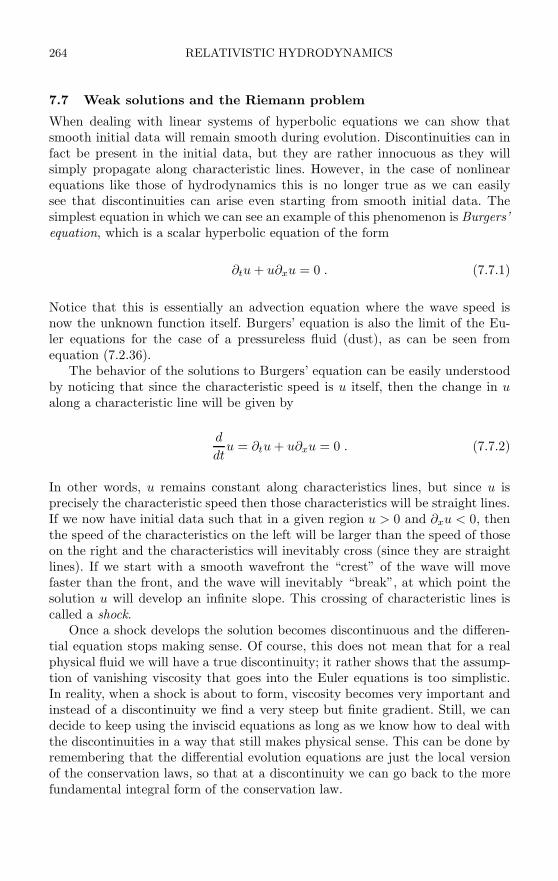
264 RELATIVISTIC HYDRODYNAMICS
7.7 Weak solutions and the Riemann problem
When dealing with linear systems of hyperbolic equations we can show thatsmooth initial data will remain smooth during evolution. Discontinuities can infact be present in the initial data, but they are rather innocuous as they willsimply propagate along characteristic lines. However, in the case of nonlinearequations like those of hydrodynamics this is no longer true as we can easilysee that discontinuities can arise even starting from smooth initial data. Thesimplest equation in which we can see an example of this phenomenon is Burgers’equation, which is a scalar hyperbolic equation of the form
∂tu + u∂xu = 0 . (7.7.1)
Notice that this is essentially an advection equation where the wave speed isnow the unknown function itself. Burgers’ equation is also the limit of the Eu-ler equations for the case of a pressureless fluid (dust), as can be seen fromequation (7.2.36).
The behavior of the solutions to Burgers’ equation can be easily understoodby noticing that since the characteristic speed is u itself, then the change in ualong a characteristic line will be given by
d
dtu = ∂tu + u∂xu = 0 . (7.7.2)
In other words, u remains constant along characteristics lines, but since u isprecisely the characteristic speed then those characteristics will be straight lines.If we now have initial data such that in a given region u > 0 and ∂xu < 0, thenthe speed of the characteristics on the left will be larger than the speed of thoseon the right and the characteristics will inevitably cross (since they are straightlines). If we start with a smooth wavefront the “crest” of the wave will movefaster than the front, and the wave will inevitably “break”, at which point thesolution u will develop an infinite slope. This crossing of characteristic lines iscalled a shock.
Once a shock develops the solution becomes discontinuous and the differen-tial equation stops making sense. Of course, this does not mean that for a realphysical fluid we will have a true discontinuity; it rather shows that the assump-tion of vanishing viscosity that goes into the Euler equations is too simplistic.In reality, when a shock is about to form, viscosity becomes very important andinstead of a discontinuity we find a very steep but finite gradient. Still, we candecide to keep using the inviscid equations as long as we know how to deal withthe discontinuities in a way that still makes physical sense. This can be done byremembering that the differential evolution equations are just the local versionof the conservation laws, so that at a discontinuity we can go back to the morefundamental integral form of the conservation law.

7.7 WEAK SOLUTIONS AND THE RIEMANN PROBLEM 265
We can use the integral form of the conservation law to define the so-calledweak solutions of the conservation law.80 To see how this works, assume thenthat we have a conservation law of the form
∂tu + ∂xF (u) = 0 . (7.7.3)
We now multiply this equation with a smooth test function φ(x, t) with compactsupport (both in space and time), and integrate over space and time∫ ∞
0
∫ ∞
−∞φ (∂tu + ∂xF ) dxdt = 0 . (7.7.4)
Integrating by parts the first term in time and the second term in space, andusing the fact the φ has compact support, we find∫ ∞
0
∫ ∞
−∞(u∂tφ + F∂xφ) dxdt = −
∫ ∞
−∞φ(x, 0)u(x, 0)dx . (7.7.5)
We now say that u is a weak solution of the conservation law if the last identityholds for all test functions φ.
To understand how weak solutions behave we must consider the so-calledRiemann problem, which is the solution corresponding to piecewise constantinitial data with a single discontinuity. As a simple example, assume that wehave initial data for Burgers’ equation of the form
u(x, 0) =
ul x < 0 ,ur x > 0 .
(7.7.6)
We can consider two distinct possibilities. Assume first that ul > ur. In this casethere is a unique weak solution corresponding to the discontinuity propagatingwith a speed s = (ul + ur)/2. To see that this is the case assume that we have adiscontinuity propagating at a speed s. We then have
d
dt
∫ xr
xl
u dx =∫ xr
xl
∂tu dx = −∫ xr
xl
∂xF (u) dx = F (ul) − F (ur) , (7.7.7)
where xl and xr are such that the discontinuity remains in the interior regionduring the time considered, and F (u) is the flux function. On the other hand,for a discontinuity propagating with speed s we clearly have
d
dt
∫ xr
xl
u dx =d
dt[(xr − xl)ur + st (ul − ur)] = s (ul − ur) , (7.7.8)
where without loss of generality we have assumed that at t = 0 the discontinuityis at x = xl. This shows that for a traveling discontinuity we should generallyhave
80The discussion that follows is based on that of [187].
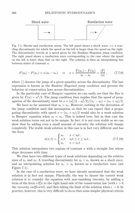
266 RELATIVISTIC HYDRODYNAMICS
Shock wave Rarefaction wave
Fig. 7.1: Shocks and rarefaction waves. The left panel shows a shock wave, i.e. a trav-eling discontinuity for which the speed on the left is larger than the speed on the right.The discontinuity travels at a speed given by the Rankine–Hugoinot jump condition.The right panel shows a rarefaction wave corresponding to the case where the speedon the left is lower than that on the right. The solution is then an interpolating linebetween states of constant u.
F (ul) − F (ur) = s (ul − ur) ⇒ s =F (ur) − F (ul)
ur − ul=
[F ][u]
, (7.7.9)
where [·] denotes the jump of a given quantity across the discontinuity. The lastexpression is known as the Rankine–Hugoinot jump condition and governs thebehavior of conservation laws across discontinuities.
In the particular case of Burgers’ equation we can easily see that the flux isgiven by F (u) = u2/2. The jump condition then implies that the speed of prop-agation of the discontinuity must be s = (u2r/2 − u2l /2)/(ur − ul) = (ur + ul)/2.
We have so far assumed that ul > ur. However, nothing in the derivation ofthe jump condition used this assumption, so that we can expect that a propa-gating discontinuity with speed s = (ur + ul)/2 would also be a weak solutionto Burgers’ equation when ul < ur. This is indeed true, but in that case theweak solution turns out not to be unique. In fact, it is not even stable as we canshow that by adding even a small amount of viscosity the solution will changecompletely. The stable weak solution in this case is in fact very different and hasthe form
u(x, t) =
⎧⎨⎩ul x < ult ,x/t ult ≤ x ≤ urt ,ur x > urt .
(7.7.10)
This solution interpolates two regions of constant u with a straight line whoseslope decreases with time.
We then have two different types of weak solutions depending on the relativesizes of ur and ul: A traveling discontinuity for ul > ur known as a shock wave,and an interpolating solution for ur > ul known as a rarefaction wave (seeFigure 7.1).
In the case of a rarefaction wave, we have already mentioned that the weaksolution is in fact not unique. Physically, the way to choose the correct weaksolution is to consider the equation with non-vanishing viscosity, by adding aterm of the form ε ∂2xu to the right hand side of the conservation law (with ε > 0the viscosity coefficient), and then taking the limit of the solution when ε → 0. Inpractice, however, this is very difficult to do so that some simpler physical criteria

7.7 WEAK SOLUTIONS AND THE RIEMANN PROBLEM 267
are required to choose among the different weak solutions. Such simpler criteriaare commonly known as entropy conditions, since they are based on an analogywith the hydrodynamic equations where the relevant physical condition we haveto apply is to say that the entropy of the fluid elements must not decrease.There are many different formulations of entropy conditions for conservationlaws, but in essence they can all be reduced to the statement that for a travelingdiscontinuity to be an “entropy solution” (i.e. a physically acceptable solution)the characteristic lines must converge at the discontinuity. If the characteristiclines instead diverge from an initial discontinuity, then the entropy solution is ararefaction wave instead.81
In the previous discussion we have assumed that we have a single non-linearscalar conservation law, in which case the solution of the Riemann problem iseither a shock wave or a rarefaction wave. There is in fact another possiblesolution known as a contact discontinuity that corresponds to the case of alinear conservation law for which the characteristic speed is constant and theinitial discontinuity simply moves along characteristic lines.
When we deal with a system of conservation laws, as opposed to a simplescalar conservation law, an extra complication arises. In this case the Rankine–Hugoinot jump condition still has the form (7.7.9), but now both [u] and [F ] arevectors so that we have in fact a set of jump conditions. However, the speed sremains a scalar, which means that not all possible jumps in the initial data areallowed as there might simply not exist a value of s that satisfies all the jumpconditions at the same time. The simplest example of this corresponds to a linearsystem of conservation laws for which the flux vector is given by F (u) = Mu,with M a constant matrix. In this case the jump conditions reduce to
M [u] = s [u] . (7.7.11)
This implies that [u] must be an eigenvector of the characteristic matrix M , withs the corresponding eigenvalue. That is, only jumps corresponding to eigenvectorsof M will result in a single propagating discontinuity, and they will move withthe corresponding characteristic speed.
What happens if we take as initial data a jump [u] that does not correspondto an eigenvector of M? After all, we are allowed to choose the initial datafreely. In this case the initial discontinuity will “split” into a group of separatediscontinuities traveling at different speeds. The original jump [u] needs to bedecomposed into a linear combination of eigenvectors of M , with each componenttraveling at its own characteristic speed. Since we are considering a linear system,all these discontinuities will correspond to simple contact discontinuities.
In the case of non-linear systems of equations like the Euler equations thesituation is more complicated, but the general idea is the same. The general
81Rarefaction waves are often also called rarefaction fans, as characteristic lines “fan out”from the discontinuity.

268 RELATIVISTIC HYDRODYNAMICS
solution of the Riemann problem involves separating an initial jump [u] into aseries of jumps, but now the different jumps might develop into shock waves thatsatisfy the entropy condition, rarefaction waves, or simple contact discontinuities.Contact discontinuities, in particular, can be expected to be present wheneverwe have a situation where a given eigenvalue λi(u) is constant along the integralcurves of the corresponding eigenvector ei(u) (i.e the curves that are tangent tothe eigenvector), that is, if
∇uλi · ei(u) = 0 , (7.7.12)
with ∇u the gradient of λi(u) with respect to the u’s (not with respect to thespatial coordinates). When this happens we say that the corresponding eigenfieldwi is linearly degenerate. If, on the other hand, the above expression is non-zerofor some i, then the corresponding eigenfield wi is called genuinely non-linear.This situation does in fact occur for the hydrodynamic equations, in which casewe can see that all three eigenfields that propagate along the flow lines arelinearly degenerate, while the sound waves are genuinely non-linear. For thelinearly degenerate fields we can have at most contact discontinuities, for whichthe density ρ0 and specific internal energy ε are discontinuous, while the pressurep and flow speed vi remain continuous.
We will not describe here in any detail the theory behind the general solutionof the Riemann problem for non-linear systems; the interested reader can see forexample [187] and references therein. It is sufficient to say that the solution tothe Riemann problem for the hydrodynamic equations in the Newtonian case iswell known, see e.g. [105]. The corresponding solution in the relativistic case wasrecently found in the case of special relativity by Marti and Muller [199], and inthe case of general relativity by Pons, Marti and Muller [229].82 A particular caseof the Riemann problem for the hydrodynamic equations, known as the shocktube problem and consisting of a fluid that is initially at rest with a discontinuityin both the density ρ0 and the specific internal energy ε (or equivalently in thepressure p), is often used as a test of numerical hydrodynamic codes.
As a simple illustration, we will consider here a propagating shock in the caseof the one-dimensional Newtonian hydrodynamic equations. The idea is to lookfor a solution corresponding to a single propagating shock moving to the rightinto a region in which the fluid is at rest. We will further assume that the fluidis an ideal gas with equation of state p = (γ − 1)ερ0. The Rankine–Hugoinotconditions in this case are
[ρ0v] = s [ρ0] , (7.7.13)[Sv + p] = s [S] , (7.7.14)
[(E + p) v] = s [E ] , (7.7.15)
82A Fortran code for computing the exact solution to the Riemann problem in the Newtoniancase can be found in the recent book by Toro [292], and another one for the relativistic casecan be found in the online version of the review paper by Marti [200].
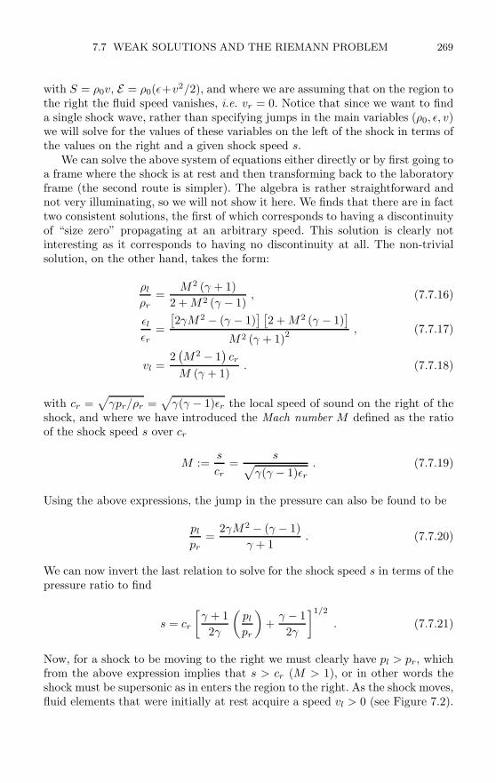
7.7 WEAK SOLUTIONS AND THE RIEMANN PROBLEM 269
with S = ρ0v, E = ρ0(ε+v2/2), and where we are assuming that on the region tothe right the fluid speed vanishes, i.e. vr = 0. Notice that since we want to finda single shock wave, rather than specifying jumps in the main variables (ρ0, ε, v)we will solve for the values of these variables on the left of the shock in terms ofthe values on the right and a given shock speed s.
We can solve the above system of equations either directly or by first going toa frame where the shock is at rest and then transforming back to the laboratoryframe (the second route is simpler). The algebra is rather straightforward andnot very illuminating, so we will not show it here. We finds that there are in facttwo consistent solutions, the first of which corresponds to having a discontinuityof “size zero” propagating at an arbitrary speed. This solution is clearly notinteresting as it corresponds to having no discontinuity at all. The non-trivialsolution, on the other hand, takes the form:
ρl
ρr=
M2 (γ + 1)2 + M2 (γ − 1)
, (7.7.16)
εl
εr=
[2γM2 − (γ − 1)
] [2 + M2 (γ − 1)
]M2 (γ + 1)2
, (7.7.17)
vl =2(M2 − 1
)cr
M (γ + 1). (7.7.18)
with cr =√
γpr/ρr =√
γ(γ − 1)εr the local speed of sound on the right of theshock, and where we have introduced the Mach number M defined as the ratioof the shock speed s over cr
M :=s
cr=
s√γ(γ − 1)εr
. (7.7.19)
Using the above expressions, the jump in the pressure can also be found to be
pl
pr=
2γM2 − (γ − 1)γ + 1
. (7.7.20)
We can now invert the last relation to solve for the shock speed s in terms of thepressure ratio to find
s = cr
[γ + 12γ
(pl
pr
)+
γ − 12γ
]1/2. (7.7.21)
Now, for a shock to be moving to the right we must clearly have pl > pr, whichfrom the above expression implies that s > cr (M > 1), or in other words theshock must be supersonic as in enters the region to the right. As the shock moves,fluid elements that were initially at rest acquire a speed vl > 0 (see Figure 7.2).
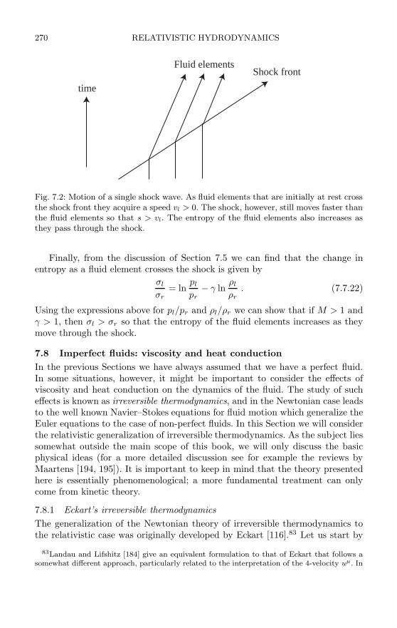
270 RELATIVISTIC HYDRODYNAMICS
time
Shock front Fluid elements
Fig. 7.2: Motion of a single shock wave. As fluid elements that are initially at rest crossthe shock front they acquire a speed vl > 0. The shock, however, still moves faster thanthe fluid elements so that s > vl. The entropy of the fluid elements also increases asthey pass through the shock.
Finally, from the discussion of Section 7.5 we can find that the change inentropy as a fluid element crosses the shock is given by
σl
σr= ln
pl
pr− γ ln
ρl
ρr. (7.7.22)
Using the expressions above for pl/pr and ρl/ρr we can show that if M > 1 andγ > 1, then σl > σr so that the entropy of the fluid elements increases as theymove through the shock.
7.8 Imperfect fluids: viscosity and heat conductionIn the previous Sections we have always assumed that we have a perfect fluid.In some situations, however, it might be important to consider the effects ofviscosity and heat conduction on the dynamics of the fluid. The study of sucheffects is known as irreversible thermodynamics, and in the Newtonian case leadsto the well known Navier–Stokes equations for fluid motion which generalize theEuler equations to the case of non-perfect fluids. In this Section we will considerthe relativistic generalization of irreversible thermodynamics. As the subject liessomewhat outside the main scope of this book, we will only discuss the basicphysical ideas (for a more detailed discussion see for example the reviews byMaartens [194, 195]). It is important to keep in mind that the theory presentedhere is essentially phenomenological; a more fundamental treatment can onlycome from kinetic theory.
7.8.1 Eckart’s irreversible thermodynamicsThe generalization of the Newtonian theory of irreversible thermodynamics tothe relativistic case was originally developed by Eckart [116].83 Let us start by
83Landau and Lifshitz [184] give an equivalent formulation to that of Eckart that follows asomewhat different approach, particularly related to the interpretation of the 4-velocity uµ. In

7.8 IMPERFECT FLUIDS 271
assuming that the state of a fluid element is always close to equilibrium so thatwe can still define a local temperature T . The state of the fluid will still bedescribed by the rest mass energy density ρ0, the specific internal energy ε, andthe 4-velocity of the fluid elements uµ, but now the pressure is assumed to includean extra contribution coming from the viscosity and known as the bulk viscouspressure Π,
p → p + Π , (7.8.1)
The non-viscous part of the pressure p is still assumed to be given by the sameequation of state as before.
The stress-energy tensor of the fluid is generalized by considering the generaldecomposition of a symmetric tensor in terms of parallel and normal projectionsalong the fluid’s 4-velocity field uµ. Doing this we find the following expressionfor the stress-energy tensor
Tµν = ρ0 (1 + ε)uµuν + (p + Π)hµν + qµuν + qµuν + πµν , (7.8.2)
with hµν = gµν + uµuν the projection operator into the fluid’s rest frame, andwhere qµ and πµν are a vector and a symmetric tensor such that
qµuµ = 0 , πµνuµ = 0 , πµµ = 0 . (7.8.3)
The vector qµ can be interpreted as the energy flux in the fluid’s frame, orin other words the heat flow. The tensor πµν , on the other hand, representsthe presence of possible anisotropic stresses (the pressure corresponds to theisotropic stresses). The quantities Π, qµ and παβ together are usually called thethermodynamic fluxes.
The dynamics of the fluid are still obtained from the conservation laws
∇µ (ρ0uµ) = 0 , ∇µT µν = 0 . (7.8.4)
Conservation of particles still leads to the same continuity equation as before,which for our purposes we will write in the form
dρ0dτ
+ ρ0∇µuµ = 0 , (7.8.5)
with d/dτ := uµ∇µ. The conservation of energy-momentum, on the other hand,is now modified because of the presence of the extra dissipative terms. In par-ticular, contracting the energy-momentum conservation with uµ results in
dρ
dτ+ (ρ + p + Π)∇µuµ + ∇µqµ + qµ duµ
dτ+ πµνσµν = 0 , (7.8.6)
the Eckart approach used here uµ corresponds to the flow of particles, while in the approach ofLandau and Lifshitz it corresponds instead to the flow of energy. Of course, in the absence ofheat conduction energy flows only with the particles, so that for a perfect fluid the two pointsof view are identical.
272 RELATIVISTIC HYDRODYNAMICS
with ρ = ρ0(1 + ε), and where σµν is the shear tensor associated with the fluidmotion, i.e the symmetric tracefree part of the projection of ∇µuν :
σµν := hαµhβ
ν
(∇(αuβ) − 1
3hαβ∇λuλ
). (7.8.7)
It is clear that the energy-momentum conservation involves the thermodynamicfluxes Π, qµ and πµν . The system of equations will therefore not be closed unlesswe can relate these fluxes to quantities associated with the fluid state, also knownas the thermodynamic potentials.
The standard approach due to Eckart starts by considering the entropy cur-rent Sµ and asking for its covariant divergence (i.e. the entropy production) tobe non-negative, in accordance with the second law of thermodynamics:
∇µSµ ≥ 0 . (7.8.8)
In the case of a perfect fluid the entropy current is simply given by Sµ = σρ0uµ,
with σ the specific entropy, and as we have seen the conservation equationsdirectly imply ∇µSµ = 0. When there is heat flow qµ, however, it contributes tothe entropy flux with a term given qµ/T (dS = dQ/T ), with T the temperatureof the fluid element, so that
Sµ = σρ0uµ +
qµ
T. (7.8.9)
Calculating the divergence and using the conservation of particles we find that
T∇µSµ = ρ0Tdσ
dτ− qµ∇µ ln T + ∇µqµ . (7.8.10)
Using now the conservation equations (7.8.5) and (7.8.6), together with the firstlaw of thermodynamics in the form
Tdσ = dε + p d
(1ρ0
), (7.8.11)
we can rewrite the entropy divergence as
T∇µSµ = −[Π ∇µuµ + qµ
(duµ
dτ+ ∇µ ln T
)+ πµνσµν
]. (7.8.12)
It is now clear that we can guarantee that this divergence will always be posi-tive if we postulate a linear relation between the thermodynamic fluxes and thethermodynamic potentials of the form
qµ = −χ
(T
duµ
dτ+ hν
µ∇νT
), (7.8.13)
Π = −ζ∇µuµ , (7.8.14)πµν = −2ησµν , (7.8.15)
with χ, ζ and η positive parameters known respectively as the coefficients of heatconduction, bulk viscosity and shear viscosity (the projection operator applied

7.8 IMPERFECT FLUIDS 273
to ∇µT in the equation for qµ is there to guarantee that qµuµ = 0). The aboveexpressions are the direct relativistic generalization of the corresponding Newto-nian expressions (except for the correction term Tduµ/dτ in the expression forqµ). We can now substitute these laws for the thermodynamic fluxes into theexpression for the stress-energy tensor and use the conservation laws to derivethe relativistic version of the Navier–Stokes equations, but we will not go intosuch detail here.
The Eckart theory just presented has a serious drawback in the sense that itis not causal. This can be seen from the fact that if a thermodynamic potentialis turned off, the corresponding flux vanishes instantaneously. To make this moreconcrete consider the problem of heat flow for a fluid at rest in flat spacetime. Inthat case we have uµ = δµ
0 and also q0 = 0, so the conservation equation (7.8.6)reduces to
∂tρ = −∑
i
∂iqi , (7.8.16)
For a fluid at rest we also have ∂tρ = ρ0∂tε = ρ0cV ∂tT , which implies
ρ0cV ∂tT = −∑
i
∂iqi . (7.8.17)
On the other hand, the heat flux is now given by qi = −χ∂iT , so that we find
ρ0cV ∂tT = χ∇2T , (7.8.18)
with ∇2 the ordinary flat space Laplacian. This is nothing more than the stan-dard heat equation. It is a parabolic equation which involves propagation ofsignals at an infinite speed, which is clearly in contradiction with the basic rela-tivistic law that no physical signal can travel faster than the speed of light. Wethen see that Eckart’s theory, though providing us with a covariant generaliza-tion of the Newtonian equations for irreversible thermodynamics, is neverthelessphysically unsatisfactory.
7.8.2 Causal irreversible thermodynamicsLet us now consider how we can modify the Eckart theory in order to recovercausality. The expression for the stress-energy tensor (7.8.2) is clearly correctsince it is just the general decomposition of a symmetric tensor in terms ofparallel and orthogonal projections to uµ. The main problem with Eckart’s theoryis that the modification of the entropy flux is just too simple. We should alsoconsider dissipative contributions to this flux, which according to kinetic theoryshould be second order in the thermodynamic fluxes. We then postulate thefollowing form for the entropy flux
Sµ = σρ0uµ +
qµ
T− uµ
2T
(β0Π2 + β1qαqα + β2παβπαβ
), (7.8.19)
with βi > 0 new thermodynamic coefficients (one can in principle also includemixed terms, but we will not consider them here). The coefficients βi need not

274 RELATIVISTIC HYDRODYNAMICS
be constant and might in fact depend on the fluid variables ρ and ε, but forsimplicity we will take them to be constant in what follows.
We can now calculate the divergence of the entropy flux (7.8.19) in the sameway as before to obtain
T∇µSµ = −Π[∇µuµ + β0
dΠdτ
+β0T
2∇µ
(uµ
T
)]−qµ
[duµ
dτ+ ∇µ ln T + β1
dqµ
dτ+
β1T
2qµ∇ν
(uν
T
)]−πµν
[σµν + β2
dπµν
dτ+
β2T
2πµν∇λ
(uλ
T
)]. (7.8.20)
Again, if we want to guarantee that this divergence is non-negative, we postulatea linear relation between the terms inside square brackets and the thermody-namic fluxes:
Π = −ζ
[∇µuµ + β0
dΠdτ
+β0T
2∇µ
(uµ
T
)], (7.8.21)
qµ = −χT
[duµ
dτ+ hν
µ∇ν ln T + β1hνµ
dqν
dτ+
β1T
2qµ∇ν
(uν
T
)], (7.8.22)
πµν = −2η
[σµν + β2h
αµhβ
ν
dπαβ
dτ+
β2T
2πµν∇λ
(uλ
T
)], (7.8.23)
with the coefficients χ, ζ and η the same as before, and where we have againintroduced the projection operator hµ
ν to guarantee that qµ and πµν remainorthogonal to uµ. The terms proportional to ∇ν (uν/T ) are usually omitted asit can be argued that they are small compared to the other terms. In that casewe can rewrite the last expressions as
τ0dΠdτ
+ Π = −ζ∇µuµ , (7.8.24)
τ1hνµ
dqν
dτ+ qµ = −χ
(T
duµ
dτ+ hν
µ∇νT
), (7.8.25)
τ2hαµhβ
ν
dπαβ
dτ+ πµν = −2ησµν , (7.8.26)
where we have introduced the shorthand
τ0 = ζβ0 , (7.8.27)τ1 = χTβ1 , (7.8.28)τ2 = 2ηβ2 . (7.8.29)
The form of the relations (7.8.24)–(7.8.26) is known as the Maxwell–Cattaneoform of the transport equations (or rather, its relativistic generalization), and
7.8 IMPERFECT FLUIDS 275
they are evolution equations instead of simple algebraic relations as before. Theparameters τi play the role of relaxation times. We now see that if a thermody-namic potential is suddenly switched off, the corresponding flux will die awayslowly in a time of order τi. The values of the τi, or correspondingly the βi, canbe roughly estimated as the mean collision time between particles. The theoryjust presented is known as the (truncated) Israel–Stewart theory of relativisticirreversible thermodynamics [167].
To see how this theory solves the causality problem, consider again heatflow in a static fluid in flat spacetime. As before, the conservation equation stillimplies
ρ0cV ∂tT = −∑
i
∂iqi . (7.8.30)
But the heat flux now satisfies the equation
τ1∂tqi = −χ∂iT − qi . (7.8.31)
This implies that
τ1ρ0cV ∂2t T = −τ1∑
i
∂i∂tqi
= χ∇2T +∑
i
∂iqi , (7.8.32)
and finallyτ1∂
2t T − χ
ρ0cV∇2T + ∂tT = 0 . (7.8.33)
Instead of the standard parabolic heat equation we have now obtained a dampedwave equation. The new equation is clearly hyperbolic, so the speed of propaga-tion is now finite.
8
GRAVITATIONAL WAVE EXTRACTION
8.1 Introduction
Gravitational waves, that is perturbations in the geometry of spacetime thatpropagate at the speed of light, are one of the most important predictions ofgeneral relativity. Though such gravitational radiation has not yet been detecteddirectly, there is strong indirect evidence of its existence in the form of thenow famous binary pulsar PSR 1913+16, whose change in orbital period overtime matches to very good accuracy the value predicted by general relativityas a consequence of the emission of gravitational waves [164, 282]. Moreover,there is every reason to believe that the new generation of large interferometricobservatories (LIGO, VIRGO, GEO 600, TAMA) will finally succeed in detectinggravitational radiation within the next few years.
Gravitational waves are one of the most important physical phenomena as-sociated with the presence of strong and dynamic gravitational fields, and assuch they are of great interest in numerical relativity. Gravitational radiationcan carry energy and momentum away from an isolated system, and it encodesinformation about the physical properties of the system itself. Predicting thegravitational wave signal coming from astrophysical systems has been one of themain themes in numerical relativity over the years, because such predictions canbe used as templates that can significantly improve the possibility of detection.
There are two main approaches to the extraction of gravitational wave in-formation from a numerical simulation. For a number of years the traditionalapproach has been based on the theory of perturbations of a Schwarzschildspacetime developed originally by Regge and Wheeler [235], Zerilli [308, 309],and a number of other authors, and later recast as a gauge invariant frameworkby Moncrief [209]. In recent years, however, it has become increasingly commonin numerical relativity to extract gravitational wave information in terms of thecomponents of the Weyl curvature tensor with respect to a frame of null vectors,using what is known as the Newman–Penrose formalism [218]. In the followingSections, I will present a brief introduction to both these approaches, and will de-scribe how we can calculate the energy and momentum radiated by gravitationalwaves in each case.
Finally, a word of warning. Unfortunately, though the main ideas and resultspresented here are well known, there are no standard conventions in either thedefinitions or the notation used for many of the concepts introduced here (inparticular, sign conventions in the definitions of Weyl scalars, spacetime invari-ants, etc., can be very different from author and to author). Here I will use of
276

8.2 PERTURBATIONS OF SCHWARZSCHILD 277
notation and definitions that are common, though not universal, and I will try tokeep the conventions consistent throughout. However, the reader is advised notto mix expressions taken from different sources without first carefully comparingthe conventions used.
8.2 Gauge invariant perturbations of Schwarzschild
In this Section we will briefly discuss some of the ideas behind the theory ofperturbations of a Schwarszchild black hole, concentrating particularly on thoseaspects that are important for gravitational wave extraction. For a more detaileddiscussion the reader is directed to the classic book by Chandrasekar [96], or therecent reviews by Kokkotas and Schmidt [175], Martel and Poisson [197], andNagar and Rezolla [211].
Let us start by assuming that we have a metric of the form
gµν = g(0)µν + hµν , (8.2.1)
where |hµν | 1 is a small perturbation, and g(0)µν is the Schwarzschild metric in
standard coordinates
g(0)µν dxµdxν = −(
1 − 2M
r
)dt2 +
(1 − 2M
r
)−1dr2 + r2dΩ2 . (8.2.2)
Because of the spherical symmetry of the background metric, it is convenientto think of the full spacetime manifold M as the product of two sub-manifolds,namely a Lorentzian two-dimensional manifold M2 associated with the coor-dinates (t, r), and the two-sphere of unit radius S2 associated with (θ, ϕ). Wecan then write our full four-dimensional manifold as M = M2 × S2. Follow-ing [211], in what follows we will make this separation explicit by using lowercase Latin indices (a, b, . . . ) to represent the coordinates in S2, and upper caseindices (A, B, . . . ) for the coordinates in M2. We can then rewrite the metric as
ds2 = gAB dxAdxB + r2Ωab dxadxb , (8.2.3)
with Ωab the metric of the unit two-sphere, Ωab = diag(1, sin2 θ). We will alsodistinguish covariant derivatives in the full spacetime from covariant derivativesin the sub-manifolds in the following way: ∇µ will represent covariant deriva-tives in M, while DA and Da will denote covariant derivatives in M2 and S2
respectively.
8.2.1 Multipole expansionAt this point it is in fact convenient to expand the metric perturbations hµν inmultipoles using spherical harmonics Y l,m(θ, ϕ), and separate those multipolesaccording to their properties with respect to parity transformations (i.e. reflec-tions through the origin) (θ, ϕ) → (π − θ, π + ϕ). We say that a given multipoleis even or polar if it transforms as (−1)l, and odd or axial if it transforms in-stead as (−1)l+1. The names even and odd come from the fact that once we

278 GRAVITATIONAL WAVE EXTRACTION
multiply with the corresponding spherical harmonic, even perturbations remainunchanged under a parity transformation, while odd perturbations change sign.The names polar and axial, on the other hand, refer to the behavior under a localchange from a right handed to a left handed basis: Polar perturbations remainunchanged, while axial perturbations again change sign.
In order to decompose hµν , we further need to introduce the scalar, vectorand tensor spherical harmonics. These tensorial properties refer only to trans-formations of coordinates in the unit sphere, so that in this sense we can regardthe components hAB as three scalars, hAb as two vectors, and hab as one tensor.Scalar harmonics are the usual functions Y l,m(θ, ϕ) (see Appendix D). Vectorharmonics, on the other hand, come in two different types. The even vector har-monics are simply defined as the gradient of the scalar harmonics on the sphere
Y l,ma := DaY l,m , (8.2.4)
while the odd vector harmonics are
X l,ma := −εa
bDbYl,m = −εac ΩcbDbY
l,m , (8.2.5)
where εab is the Levi–Civita completely antisymmetric tensor on the two-sphere(εθϕ = −εϕθ = Ω1/2 = sin θ).
Similarly, we can define tensor harmonics of even and odd type. Even tensorharmonics can be constructed in two ways, either by multiplying the scalar har-monics with the angular metric Ωab, or by taking a second covariant derivativeof the Y l,m:
ΩabYl,m , DaDbY
l,m . (8.2.6)
However, there is a subtle point here. It turns out that these functions do notform a linearly independent set, so instead of the DaDbY
l,m, it is better to usethe so-called Zerilli–Mathews tensor harmonics defined as
Z l,mab := DaDbY
l,m +12
l (l + 1)ΩabYl,m . (8.2.7)
Remembering now that the scalar spherical harmonics are eigenfunctions of theLaplace operator on the sphere, that is
DaDaY l,m =[∂2θ +
1sin2 θ
∂2ϕ + cot θ ∂θ
]Y l,m = −l (l + 1)Y l,m , (8.2.8)
we can easily see that the Zerilli–Mathews tensor harmonics Zl,mab are in fact
traceless. We can also show that the divergence of Zl,mab is given by
DbZ l,mab = −1
2(l − 1)(l + 2) Y l,m
a , (8.2.9)
where in order to derive this expression we need to use the fact that the Riccitensor for the two-sphere is just equal to the angular metric Rab = Ωab.

8.2 PERTURBATIONS OF SCHWARZSCHILD 279
Odd parity tensor harmonics, on the other hand, can be constructed in onlyone way, namely
X l,mab =
12
(DaX l,m
b + DbXl,ma
). (8.2.10)
From the definition of the X l,ma we can easily see that the odd tensor harmonics
are again traceless. We also find for the divergence of X l,mab
DbX l,mab = −1
2(l − 1)(l + 2) X l,m
a . (8.2.11)
At this point it is important to mention the fact that, since Y 00 is a constant,both vector and tensor harmonics vanish for l = 0. On the other hand, for l = 1the vector harmonics do not vanish, but the tensor harmonics can still be easilyshown to vanish from the explicit expressions for Y 1m. This means that vectorharmonics are only non-zero for l ≥ 1, and tensor harmonics for l ≥ 2. The scalarmode with l = 0 can be interpreted as a variation in the mass of the Schwarzschildspacetime, the odd vector mode with l = 1 as an infinitesimal contribution to theangular momentum (the “Kerr” mode [252]), while the scalar and even vectormodes with l = 1 are just gauge [197]. Also, for any given value of l, the indexm can only take integer values from −l to l.
Having defined the vector and tensor harmonics, the perturbed metric isexpanded in multipoles, and separated into its even sector given by(
hl,mAB
)(e)= H l,m
AB Y l,m , (8.2.12)(hl,m
Ab
)(e)= H l,m
A Y l,mb , (8.2.13)(
hl,mab
)(e)= r2
(K l,m ΩabY
l,m + Gl,mZ l,mab
), (8.2.14)
and its odd sector given by (hl,m
AB
)(o)= 0 , (8.2.15)(
hl,mAb
)(o)= hl,m
A X l,mb , (8.2.16)(
hl,mab
)(o)= hl,m X l,m
ab , (8.2.17)
where the coefficients (H l,mAB , H l,m
A , K l,m, Gl,m, hl,mA , hl,m) are in general functions
of r and t.The vector and tensor harmonics introduced above are related to the spin-
weighted spherical harmonics defined in Appendix D. In order to find this rela-tion, consider the two unit complex vectors (these vectors will appear again inSection 8.5 when we discuss the Newman–Penrose formalism)

280 GRAVITATIONAL WAVE EXTRACTION
ma :=1√2
(1, i sin θ) , ma :=1√2
(1,−i sin θ) , (8.2.18)
where z denotes the complex conjugate of z. In terms of (ma, ma), we find thatthe vector harmonics Y l,m
a and X l,ma can be written as
Y l,ma =
(l(l + 1)
2
)1/2 [−1Y l,m ma − 1Y
l,m ma
], (8.2.19)
X l,ma = −i
(l(l + 1)
2
)1/2 [−1Y l,m ma + 1Y
l,m ma
]. (8.2.20)
Similarly, for the tensor harmonics we find
Z l,mab =
12
((l + 2)!(l − 2)!
)1/2 [−2Y l,m mamb + 2Y
l,m mamb
], (8.2.21)
X l,mab = − i
2
((l + 2)!(l − 2)!
)1/2 [−2Y l,m mamb − 2Y
l,m mamb
], (8.2.22)
where in order to derive the last expressions we have again used the fact thatthe scalar harmonics are eigenfunctions of the Laplace operator on the sphere.Notice again that, since the spin-weighted harmonics are defined only for l > |s|,the above expressions are consistent with the fact that vector harmonics startwith l = 1 and tensor harmonics with l = 2.
8.2.2 Even parity perturbations
As we have seen, even parity perturbations are characterized by the coefficients(H l,m
AB , H l,mA , K l,m, Gl,m). These coefficients are clearly coordinate dependent,
and in particular change under infinitesimal coordinate transformations, i.e.gauge transformations, of the form
xµ → xµ + ξµ , (8.2.23)
with |ξµ| << 1. Such gauge transformations were already discussed in Chapter 1,and we can easily show that they result in a change in the metric perturbationof the form
hµν → hµν −∇µξν −∇νξµ . (8.2.24)
The only difference between this expression and that of Chapter 1 is the fact thatwe now have a non-trivial background metric and, as a consequence, the gaugetransformation involves covariant derivatives with respect to the backgroundmetric.
It turns out that we can in fact construct gauge invariant combinations ofthe coefficients (H l,m
AB , H l,mA , K l,m, Gl,m). In order to do this, let us consider an

8.2 PERTURBATIONS OF SCHWARZSCHILD 281
even-parity gauge transformation ξµ = (ξA, ξa), which can be expanded in termsof scalar and vector harmonics as
ξA =∑l,m
El,mA Y l,m , ξa =
∑l,m
El,mY l,ma , (8.2.25)
We now need to use this expression to find the transformation of the coefficientscorresponding to an even perturbation. We start from the expression for themixed Christoffel symbols which can be easily shown to be
ΓABc = Γa
BC = 0 , ΓAbc = −rrAΩbc , Γa
Bc =rB
rδac , (8.2.26)
where rA := DAr. Using this we find that
∇AξB =∑l,m
(DAEl,m
B
)Y l,m , (8.2.27)
∇Aξb =∑l,m
(DAEl,m − rA
rEl,m
)Y l,m
b , (8.2.28)
∇aξB =∑l,m
(El,m
B − rB
rEl,m
)Y l,m
a , (8.2.29)
∇aξb =∑l,m
[(DaY l,m
b
)El,m + rΩab rCEl,m
C Y l,m]
. (8.2.30)
The gauge transformation of (H l,mAB , H l,m
A , K l,m, Gl,m) then takes the form
H l,mAB → H l,m
AB − DAEl,mB − DBEl,m
A , (8.2.31)
H l,mA → H l,m
A − El,mA − DAEl,m +
2rA
rEl,m , (8.2.32)
K l,m → K l,m − 2r
rAEl,mA +
l(l + 1)r2
El,m , (8.2.33)
Gl,m → Gl,m − 2r2
El,m . (8.2.34)
We can now use these results to construct gauge invariant combinations of coef-ficients. Two such invariant combinations are [143]
K l,m := K l,m +12
l(l + 1) Gl,m − 2r
rAεl,mA , (8.2.35)
H l,mAB := H l,m
AB − DAεl,mB − DBεl,m
A , (8.2.36)
withεl,m
A := H l,mA − 1
2r2DAGl,m . (8.2.37)
Instead of looking for gauge invariant combinations we can choose to workon a specific gauge. For example, from the transformations above it is clear that

282 GRAVITATIONAL WAVE EXTRACTION
we can choose El,m and El,mA such that Gl,m = H l,m
A = 0. This is known asthe Regge–Wheeler gauge, and with that choice we clearly has K l,m = K l,m,H l,m
AB = H l,mAB .
In terms of the gauge invariant perturbations K l,m and H l,mAB we define the
so-called Zerilli–Moncrief master function as
Ψl,meven :=
2r
l(l + 1)
[K l,m +
2Λ
(rArBH l,m
AB − rrADAK l,m)]
, (8.2.38)
with Λ := (l − 1)(l + 2) + 6M/r. The importance of this definition comes fromthe fact that using the perturbed Einstein field equations we can show thatΨl,meven obeys a simple wave-like equation known as the Zerilli equation, or more
generally the even-parity master equation:
∂2t Ψl,meven − ∂2r∗Ψl,m
even + V l,meven Ψl,m
even = Sl,meven , (8.2.39)
with r∗ the tortoise radial coordinate defined as r∗ := 1 + 2M ln (r/2M − 1),and where V l,m
even and Sl,meven are a potential and a source term that depend on r
and l, but whose explicit expression is not important for the present discussion(but see e.g. [197]).
The Zerilli equation is specially useful in the frequency domain, for whichwe assume that Ψl,m
even(t, r) = exp(iωnt)F (r), with ωn some complex frequency.Substituting this into the Zerilli equation, and imposing boundary conditionssuch that we have purely outgoing waves at spatial infinity (r∗ → ∞) and purelyingoing waves at the black hole horizon (r∗ → −∞), we obtain an eigenvalueproblem for the complex frequencies ωn. The different values of ωn found in thisway give us the allowed frequencies of oscillation of the perturbations (the realpart of ωn) and their corresponding decay rates (the imaginary part of ωn). Suchsolutions are known as the quasi-normal modes of the black hole.
We will not go into a discussion of the quasi-normal modes of Schwarzschild,but we will mention a few important points. First, all the resulting modes aredamped, with the higher frequency (shorter wavelength) modes damped thefastest. The so-called fundamental mode l = 2, which is often the most exitedand decays the slowest, has a wavelength of Re(ω) ∼ 16.8M . When the blackhole is excited (e.g. by throwing matter into it), it behaves much like a bell inthe sense that it oscillates at its characteristic frequencies, losing energy in theform of gravitational waves, and eventually settling down to a stationary state.Such behavior is known as “ringing”, and we typically find that the late timegravitational wave signal coming from a system that has collapsed to a singleblack hole can always be matched to a superposition of the quasi-normal modesof the final black hole. The reader interested in studying these issues in moredetail is directed to references [96, 175].

8.2 PERTURBATIONS OF SCHWARZSCHILD 283
8.2.3 Odd parity perturbations
Just as we did for the even perturbations, we can also construct gauge invariantquantities for the case of odd perturbations. We then start by considering anodd gauge transformation ξµ = (ξA, ξa), which can now be expanded in terms ofscalar and vector harmonics as
ξA = 0 , ξa =∑l,m
El,mX l,ma . (8.2.40)
Using this we now find that
∇AξB = 0 , (8.2.41)
∇Aξb =∑l,m
(DAEl,m − rA
rEl,m
)X l,m
b , (8.2.42)
∇aξB = −∑l,m
rB
rEl,mX l,m
a , (8.2.43)
∇aξb =∑l,m
(DaX l,m
b
)El,m , (8.2.44)
with rA the same as before. The coefficients (hl,mA , hl,m) for the odd perturbations
then transform as
hl,mA → hl,m
A − DAEl,m +2rA
rEl,m , (8.2.45)
hl,m → hl,m − 2El,m . (8.2.46)
Just as before, we can use these transformations to construct a gauge invariantquantity in the following way [143]
hl,mA := hl,m
A − 12
DAhl,m +rA
rhl,m . (8.2.47)
Notice that, from the transformations above, it is clear that we can always chooseEl,m such that hl,m = 0, in which case we will have hl,m
A = hl,mA , corresponding
to the Regge–Wheeler gauge.In terms of hl,m
A we define the Cunningham–Price–Moncrief master function:
Ψl,modd :=
2r
(l − 1)(l + 2)εAB
[DAhl,m
B − 2rA
rhl,m
B
]=
2r
(l − 1)(l + 2)εAB
[DAhl,m
B − 2rA
rhl,m
B
]. (8.2.48)
The second equality shows that Ψl,modd in fact depends only on hl,m
A and not onhl,m (the contributions from hl,m cancel when contracted with the εAB), but it
284 GRAVITATIONAL WAVE EXTRACTION
is nevertheless gauge invariant (we can also change DAhl,mB for ∂Ahl,m
B since theChristoffel symbols also drop out, but we leave the covariant derivative to showexplicitly that Ψl,m
odd is covariant).Again, using the perturbed Einstein field equations we can show that Ψl,m
odd
obeys a wave-like equation of the form
∂2t Ψl,modd − ∂2r∗Ψl,m
odd + V l,modd Ψl,m
odd = Sl,modd , (8.2.49)
where again V l,modd and Sl,m
odd are a potential and a source term whose explicitexpression we will not write here. The above equation is known as the Regge–Wheeler equation, or more generally the odd-parity master equation.
8.2.4 Gravitational radiation in the TT gauge
We now need to relate the gauge invariant perturbations introduced in the lasttwo sections with the gravitational waves amplitudes in the transverse-traceless(TT) gauge, h+ and h×. As we will see in Section 8.9, this will allow us tocompute the energy and momentum carried by the gravitational waves.
Consider first the even parity perturbations. If asymptotically we approachthe TT gauge then we will find that hAB and hAb decay much faster than hab.According to the multiple expansion we can then ignore the coefficients H l,m
AB andH l,m
A , and concentrate only on K l,m and Gl,m. Consider now an orthonormalangular basis (eθ, eϕ). From the discussion on gravitational waves of Chapter 1we see that in this basis we will have
h+ =12(hθθ − hϕϕ
)=
12r2
(hθθ − hϕϕ
sin2 θ
), (8.2.50)
h× = hθϕ =hθϕ
r2 sin θ. (8.2.51)
Using now the multiple expansion we find that this implies
(h+)l,meven =
Gl,m
2
(Zl,m
θθ − Zl,mϕϕ
sin2 θ
), (8.2.52)
(h×)l,meven = Gl,m
(Z l,m
θϕ
sin θ
). (8.2.53)
On the other hand, from the traceless condition we have
Ωab(K l,mΩabY
l,m + Gl,mZ l,mab
)= 0 . (8.2.54)
But we have already seen that Z l,mab is itself traceless, so the last condition reduces
to K l,m = 0. The Zerilli–Moncrief function defined in (8.2.38) then simplifies to
Ψl,meven = r Gl,m . (8.2.55)
8.2 PERTURBATIONS OF SCHWARZSCHILD 285
We then see that the contribution from the even perturbations to the TT metricfunctions is given in terms of Ψl,m
even as
(h+)l,meven =
Ψl,meven
2r
(Z l,m
θθ − Zl,mϕϕ
sin2 θ
)
=Ψl,meven
r
[∂2
∂θ2+
12
l(l + 1)]
Y l,m , (8.2.56)
(h×)l,meven =
Ψl,meven
r
(Z l,m
θϕ
sin θ
)
=Ψl,meven
r
(im
sin θ
)[∂
∂θ− cot θ
]Y l,m , (8.2.57)
where we used the fact that ∂ϕY l,m = imY l,m.
Consider now the odd perturbations, for which we have
(h+)l,modd =
hl,m
2r2
(X l,m
θθ − X l,mϕϕ
sin2 θ
), (8.2.58)
(h×)l,modd =
hl,m
r2
(X l,m
θϕ
sin θ
). (8.2.59)
We now need to relate hl,m to Ψl,modd. In this case, however, we can not just
ignore hl,mA in favor of hl,m since from the definition of Ψl,m
odd, equation (8.2.48),we see that it in fact depends only on hl,m
A and not on hl,m. However, in the TTgauge these quantities are related to each other. In order to see this, considerthe transverse condition on hµa:
∇µhµa = 0 . (8.2.60)
Using now the multipole expansion and the expression for the mixed Christoffelsymbols we find that this implies
X l,ma DA
(r2hl,m
A
)+ hl,mDbX l,m
ab = 0 . (8.2.61)
Substituting now the divergence of X l,mab from equation (8.2.11), this becomes
DA(r2hl,m
A
)=
12
(l − 1)(l + 2) hl,m . (8.2.62)
Now, remember also that in the TT gauge we have the extra freedom of takinghµν to be purely spatial, so that hµ0 = 0. Also, asymptotically the metric gAB
is just the Minkowski metric. The previous expression then reduces to
286 GRAVITATIONAL WAVE EXTRACTION
∂r
(r2hl,m
r
)=
12
(l − 1)(l + 2) hl,m . (8.2.63)
Moreover, we can also rewrite expression (8.2.48) for Ψl,modd as
Ψl,modd =
2r
(l − 1)(l + 2)∂th
l,mr . (8.2.64)
Collecting results we find that
∂r
(rΨl,m
odd
)=
2(l − 1)(l + 2)
∂t∂r
(r2hl,m
r
)= ∂th
l,m . (8.2.65)
For an outgoing wave we have ∂thl,m ∼ −∂rh
l,m, so that we can integrate theabove expression to find
hl,m ∼ −r Ψl,modd . (8.2.66)
We can then rewrite the odd metric perturbations as
(h+)l,modd = −Ψl,m
odd
2r
(X l,m
θθ − X l,mϕϕ
sin2 θ
)
= −Ψl,modd
r
(im
sin θ
)[∂
∂θ− cot θ
]Y l,m , (8.2.67)
(h×)l,modd = −Ψl,m
odd
r
(X l,m
θϕ
sin θ
)
=Ψl,modd
r
[∂2
∂θ2+
12
l(l + 1)]
Y l,m . (8.2.68)
The full TT coefficients h+ and h× then take the final form
h+ =12r
∑l,m
[Ψl,meven
(Zl,m
θθ − Zl,mϕϕ
sin2 θ
)− Ψl,m
odd
(X l,m
θθ − X l,mϕϕ
sin2 θ
)], (8.2.69)
h× =1r
∑l,m
[Ψl,meven
(Z l,m
θϕ
sin θ
)− Ψl,m
odd
(X l,m
θϕ
sin θ
)]. (8.2.70)
Notice that since the above expressions involve only tensor harmonics, the sumover l starts with l = 2, while the sum over m goes from −l to l. In what followswe will always assume this to be the case, and will never write the summationlimits explicitly.84
84For summations involving coefficients with indices l′ = l±1 and m′ = m±1, such as thosethat will appear when discussing the linear and angular momentum carried by gravitationalwaves in Section 8.9, we should only remember that the expansion coefficients vanish wheneverl′ < 2 and |m′| > l.

8.2 PERTURBATIONS OF SCHWARZSCHILD 287
Notice that while the functions (Ψl,meven, Ψ
l,meven) are in general complex, the
TT coefficients h+ and h× must be real. Using the properties of the sphericalharmonics under complex conjugation we can easily show that this implies
Ψl,meven = (−1)m Ψl,−m
even , Ψl,modd = (−1)m Ψl,−m
odd . (8.2.71)
We can also rewrite the above expressions for h+ and h× in terms of spin-weighted spherical harmonics. For this it is in fact more convenient to considerthe complex combination H := h+ − ih×, for which we find
H =12r
∑l,m
((l + 2)!(l − 2)!
)1/2 [Ψl,meven + iΨl,m
odd
]−2Y l,m . (8.2.72)
Before leaving this section it is important to mention one very common con-vention used in numerical relativity. We start by considering a different oddmaster function originally introduced by Moncrief [209]:
Ql,mM :=
2rAhl,mA
r=
2rA
r
(hl,m
A − 12
DAhl,m +rA
rhl,m
). (8.2.73)
Notice that with this definition Ql,mM is clearly gauge invariant and a scalar.
The Moncrief function just defined has traditionally been the most commonchoice for studying odd perturbations of Schwarzschild, and because of this,many existing numerical implementations use this function instead of Ψl,m
odd. Us-ing again (8.2.63), we can show that asymptotically and in the TT gauge Ql,m
M
reduces to
Ql,mM ∼ − 2r
(l − 1)(l + 1)∂2rhl,m
r ∼ − 2r
(l − 1)(l + 1)∂2t hl,m
r , (8.2.74)
so thatQl,mM ∼ −∂tΨ
l,modd . (8.2.75)
We finally introduce the following rescaling
Ql,meven :=
((l + 2)!2(l − 2)!
)1/2Ψl,meven , (8.2.76)
Ql,modd :=
((l + 2)!2(l − 2)!
)1/2Ql,mM = −
((l + 2)!2(l − 2)!
)1/2∂tΨ
l,modd . (8.2.77)
Again, the fact that h+ and h× are real implies that
Ql,meven = (−1)m Ql,−m
even , Ql,modd = (−1)m Ql,−m
odd . (8.2.78)
In terms of Ql,meven and Ql,m
odd we now find for the complex coefficient H :
H =1√2r
∑l,m
[Ql,meven − i
∫ t
−∞Ql,modd dt′
]−2Y l,m . (8.2.79)
288 GRAVITATIONAL WAVE EXTRACTION
8.3 The Weyl tensorA second approach to the extraction of gravitational wave information is basedon definition of the Weyl tensor. In a general n-dimensional space the Riemanntensor Rα
βµν has n4 components, but all its symmetries reduce the number ofindependent components to only n2(n2−1)/12. On the other hand, the Ricci ten-sor Rµν := Rα
µαν , being symmetric in its two indices, has in general n(n + 1)/2independent components. Notice that, in two dimensions, both the Riemann andRicci tensors have only one independent component so they are both proportionalto the scalar curvature R, while in three dimensions they both have six inde-pendent components, and the Riemann is proportional to the Ricci.85 However,for dimensions larger than three, as in the case of the four-dimensional physicalspacetime, the Riemann tensor has more independent components than the Riccitensor, which implies that it can be decomposed in terms of the Ricci and anadditional object known as the Weyl tensor, and defined for an n-dimensionalspace as
Cαβµν := Rαβµν − 2n − 2
[gα[µRν]β − gβ[µRν]α
]+
2(n − 1)(n − 2)
gα[µgν]βR . (8.3.1)
From the definition above it is clear that the Weyl tensor has the same symme-tries as the Riemann tensor. Moreover, we can also easily see that it is traceless:
Cαµαν = 0 . (8.3.2)
In n dimensions, the Weyl tensor has n(n + 1)(n + 2)(n − 3)/12 independentcomponents (i.e. 10 independent components in four dimensions), and vanishesidentically for n ≤ 3. Notice that if we are in vacuum, and the Einstein fieldequations hold, then the Ricci tensor vanishes and the Riemann and Weyl tensorscoincide.
Another important property of the Weyl tensor is related to its behaviorunder conformal transformations of the form
gij = Ω gij . (8.3.3)
It turns out that even though, under such a transformation, the two metrics gij
and gij have, in general, different Riemann curvature tensors, they neverthelesshave the same Weyl tensor:
Cαβµν = Cα
βµν . (8.3.4)
In other words, the Weyl tensor is conformally invariant, and because of this itis often called the conformal curvature tensor.
85The formula n(n+1)/2 for the number of independent components of the Ricci tensor doesnot apply for dimensions less than three, since being constructed from the Riemann tensor,the Ricci tensor can not have more independent components. In the particular case of only onedimension the Riemann tensor in fact vanishes, i.e. a single line has no intrinsic curvature.

8.3 THE WEYL TENSOR 289
Let us now concentrate in the four-dimensional physical spacetime. We canwrite the Bianchi identities (1.10.2) in terms of the Weyl tensor as
∇αCαβµν = ∇[µRν]β +
16
gβ[µ∇ν]R , (8.3.5)
which through the Einstein field equations reduces to
∇αCαβµν = 8π
[∇[µTν]β +
13
gβ[µ∇ν]T
]. (8.3.6)
We then see that, in vacuum, the Weyl tensor has zero divergence.Given an arbitrary timelike unit vector nµ, we define the electric Eµν and
magnetic Bµν parts of the Weyl tensor as
Eµν := nαnβ Cαµβν , (8.3.7)Bµν := nαnβ C∗
αµβν , (8.3.8)
where C∗αµβν is the so-called dual Weyl tensor
C∗αβµν :=
12
Cαβλσ ελσµν , (8.3.9)
with εαβµν the Levi–Civita completely antisymmetric tensor. The word “dual”refers in general to a transformation such that when applied twice it returns youto the original situation with at most a change of sign (or a factor ±i). In thiscase we find that
C∗∗αβµν = −Cαβµν . (8.3.10)
To prove this we need to use the fact that the contraction of two Levi–Civitasymbols in an n-dimensional space is given in general by
εµ1···µpα1···αn−pεµ1···µpβ1···βn−p = (−1)sp! (n − p)! δ[α1β1
· · · δαn−p]βn−p
, (8.3.11)
where s is the number of negative eigenvalues of the metric (which in the caseof a Lorentzian spacetime is 1).
The names of the electric and magnetic tensors come from the fact that whenwe rewrite the Bianchi identities in terms of Eij and Bij , the resulting equationshave the same structure as Maxwell’s equations.
The symmetries of Weyl imply that the electric and magnetic tensors areboth symmetric, traceless, and spacelike in the sense that
nµEµν = 0 , nµBµν = 0 . (8.3.12)
The symmetry of the magnetic part is not evident from its definition, but it isin fact not difficult to prove (see below). This means that both Eµν and Bµν
have five independent components, giving a total of 10. Since this is precisely

290 GRAVITATIONAL WAVE EXTRACTION
the number of independent components of the Weyl tensor, we can expect tobe able to express Cαβµν in terms of the electric and magnetic tensors. This isindeed the case, and the Weyl tensor can in general be written as
Cαβµν = 2[lα[µEν]β − lβ[µEν]α − n[µBν]λελ
αβ − n[αBβ]λελµν
], (8.3.13)
withlµν := gµν + 2nµnν . (8.3.14)
If we now take the vector nµ to be the unit normal vector to the spacelikehypersurfaces in the 3+1 formalism, we can use the Gauss–Codazzi and Codazzi–Mainardi equations (2.4.1) and (2.4.2) to write the electric and magnetic tensorsin 3+1 language as
Eij = Rij + KKij − KimKmj − 4π
[Sij +
γij
3(4ρ − S)
], (8.3.15)
Bij = εimn [DmKnj − 4πγjmjn] , (8.3.16)
with ρ, Sij and ji the energy density, stress tensor and momentum density mea-sured by the Eulerian observers, and where εijk is now the Levi–Civita tensor inthree dimensions which is constructed from εαβµν as 86
εβµν = nαεαβµν . (8.3.17)
Notice that the Hamiltonian constraint (2.4.10) guarantees that the trace of Eij
vanishes, while the trace of Bij can be seen to vanish trivially from the anti-symmetry of the Levi–Civita tensor. In contrast, the symmetry of Eij is evident,while the symmetry of Bij comes about through the momentum constraints. Tosee this consider the contraction of Bij with the Levi–Civita tensor
εijaBij = εijaεimn
[DmKn
j − 4πδmj jn
]. (8.3.18)
Now, from the general expression for the contraction of two Levi–Civita symbolsgiven above we find
εiabεimn = δamδb
n − δbmδa
n , (8.3.19)
which implies
εijaBij =(δjmδa
n − δamδj
n
) [DmKn
j − 4πδmj jn
]= [DmKa
m − DaK − 8πja] = 0 , (8.3.20)
where the last equality follows from the momentum constraints (2.4.11). Thisshows that Bij is indeed a symmetric tensor.
86The definition of the three-dimensional εijk is one of those few places where it actuallymakes a difference to define the spacetime coordinates as (x0, x1, x2, x3) = (t, x, y, z) or as(x1, x2, x3, x4) = (x, y, z, t). Notice that, even in Minkowski spacetime, if we take the firstchoice we find ε123 = nµεµ123 = ε0123 = 1, while with the second choice we have insteadε123 = nµεµ123 = ε4123 = −1. So that when we work with (x1, x2, x3, x4) = (x, y, z, t) it is infact better to define εαβµ := nνεαβµν .
8.4 THE TETRAD FORMALISM 291
8.4 The tetrad formalism
Up to this point we have assumed that the components of tensors are alwaysexpressed in terms of a coordinate basis eµ. However, in many cases it isparticularly useful to work instead with a basis that is independent of the co-ordinates. In particular, the use of such non-coordinate basis is at the heart ofmany important theoretical advances in relativity theory and, as we will see inthe next Section, forms the foundation of the Newman–Penrose formalism.
At every point of spacetime, consider a set of four linearly independent vectorse(a), where the Latin index in parenthesis identifies the different vectors (herewe will modify our usual convention and allow Latin indices inside parenthesisto take values (0, 1, 2, 3)). Moreover, assume that these vectors are such that
e(a) · e(b) = η(a)(b) , (8.4.1)
with η(a)(b) a constant matrix independent of the position in spacetime. In sucha case the set of vectors e(a) is called a tetrad. Notice that the η(a)(b) arenothing more than the components of the metric tensor in the tetrad basis.In the particular case when the tetrad is orthonormal, η(a)(b) reduces to theMinkowski tensor, but for the moment we will only assume that it is constant.
Since the vectors e(a) are linearly independent, it is clear that the matrixη(a)(b) can be inverted. We denote its inverse by η(a)(b), so that we have
η(a)(c)η(c)(b) = δ(a)(b) . (8.4.2)
Let us now introduce a new set of vectors e (a) defined as
e (a) = η(a)(b)e (a). (8.4.3)
From this definition it is easy to show that these vectors are such that
e (a) · e(b) = δ(a)(b) . (8.4.4)
Figure 8.1 shows a graphical representation of the relationship between the twosets of vectors.
The tetrad vectors e(a) can be used as a basis, so that we can express anyarbitrary vector v as
v = v(a)e(a) . (8.4.5)
In order to solve for v(a), we multiply both sides of the above expression withe (b) to obtain
e (b) · v = e (b) ·(v(a)e(a)
)= v(a)
(e (b) · e(a)
). (8.4.6)
Using now (8.4.4) we findv(a) = v · e (a) . (8.4.7)

292 GRAVITATIONAL WAVE EXTRACTION
e(1)
e(2)
e (1)
e (2)
Fig. 8.1: Starting from the two vectors (e(1), e(2)), we construct a new vectors (e (1), e (2))
such that e(1) · e (2) = 0, e(2) · e (1) = 0, e(1) · e (1) = 1, e(2) · e( 2) = 1.
The same can clearly be done with the vectors e (a); we then have in general
v = v(a)e(a) = v(a)e(a) , (8.4.8)
withv(a) = v · e (a) , v(a) = v · e(a) . (8.4.9)
This implies, in particular, that the scalar product of any two vectors v and utakes the form
v · u = vµuµ = v(a)u(a) . (8.4.10)
The scalar product can then be expressed either as the contraction of the co-variant and contra-variant spacetime components, or the contraction of the cor-responding components in terms of the tetrad.
Using the above results we also find that
v = v(a)e(a) = (v · e (a))e(a) = (vµe (a)µ)(e(a)νeν) , (8.4.11)
where we have expressed the tetrad vector e(a) in terms of the coordinate basiseµ. The previous equation implies that
e(a)µ e(a)ν = δν
µ . (8.4.12)
Together, equations (8.4.4) and (8.4.12) can be written as
e(a)µ e(b)µ = δ
(b)(a) , (8.4.13)
e(a)µ e(a)ν = δµ
ν . (8.4.14)
A very important consequence of this is the following
gµν = e(a)µ e(a)ν = η(a)(b)e(a)µ e(b)µ . (8.4.15)
This expression allows us to recover the metric components in the coordinateframe in terms of the components of the tetrad vectors.
8.4 THE TETRAD FORMALISM 293
There are several advantages to the use of tetrads instead of a coordinatebasis. In the first place, the components of the metric tensor are constant in atetrad basis. But more important, since the tetrad is defined independently ofthe coordinates, the tetrad components of any geometric object behave as scalarswith respect to coordinate changes.
We can also show that it is possible to go back and forth from the coordinatecomponents of any tensor to its tetrad components by simply contracting theappropriate indices with the tetrad itself. For example, for a rank 2 tensor wehave
T(a)(b) = Tµνe(a)µe(b)
ν , Tµν = T(a)(b)e(a)
µe(b)ν . (8.4.16)
In general, the tetrad vectors can be used to define directional derivatives ofa scalar function f as
f,(a) := e(a)µ∂µf . (8.4.17)
Since the tetrad components of a vector are scalar functions, we can also find thedirectional derivatives of an arbitrary vector A = A(a)e(a) in the following way
A(a),(b) := e(b)µ∂µA(a) = e(b)
µ∂µ
(e(a)
νAν
)= e(b)
µ(e(a)
ν∂µAν + Aν∂µe(a)ν)
. (8.4.18)
In this expression, the partial derivatives can in fact be changed for covariantderivatives since the Christoffel symbols cancel out. We can then rewrite thedirectional derivative as
A(a),(b) = e(a)νe(b)
µ∇µAν + e(b)µe(c)
νA(c)∇µe(a)ν . (8.4.19)
We now define the Ricci rotation coefficients as
γ(a)(b)(c) := e(a)µe(c)
ν∇νe(b)µ , (8.4.20)
so the directional derivative takes the final form
A(a),(b) = e(a)νe(b)
µ∇µAν + γ(c)(a)(b)A(c) . (8.4.21)
From the definition of the Ricci rotation coefficients it is also easy to show that
∇(a) e(b) ≡ e(a)µ∇µe(b) = γ(c)(b)(a)e(c) . (8.4.22)
We then see that the γ(c)(b)(a) are nothing more than the connection coefficientsin the tetrad basis. Notice, however, that since the tetrad is not a coordinatebasis, in general we will have that
γ(c)(a)(b) = γ(c)(b)(a) . (8.4.23)
On the other hand, from the fact that e(a) ·e(b) = η(a)(b), with η(a)(b) constant,we can see that
294 GRAVITATIONAL WAVE EXTRACTION
∇µ
(e(a)
νe(b)ν)
= 0 ⇒ e(a)ν∇µe(b)ν = −e(b)ν∇µe(a)
ν , (8.4.24)
which impliesγ(a)(b)(c) = −γ(b)(a)(c) . (8.4.25)
The Ricci rotation coefficients are therefore antisymmetric in their first two in-dices. This means that in a general four-dimensional spacetime there are only 24independent γ(a)(b)(c), which is in contrast with the 40 independent componentsof the Christoffel symbols Γα
µν in a coordinate basis. This is another advantageof the tetrad approach.
We now define the intrinsic derivative of a vector A as
A(a)|(b) := e(a)µe(b)
ν∇νAµ = A(a),(b) − γ(c)(a)(b)A(c) . (8.4.26)
The intrinsic derivative is in fact nothing more than the covariant derivativeexpressed in the tetrad basis. Equation (8.4.26) can be generalized in a straight-forward way to tensors of arbitrary rank.
The final ingredient is the expression for the Riemann curvature tensor intetrad components. Starting from the Ricci identity for the tetrad vectors (equa-tion (1.9.3)):
Rαβµν e(b)
β = ∇µ∇νe(b)α −∇ν∇µe(b)
α , (8.4.27)
and projecting onto the tetrad
R(a)(b)(m)(n) = Rαβµνe(a)αe(b)
βe(m)µe(n)
ν , (8.4.28)
we find, after some algebra, that
R(a)(b)(m)(n) = γ(a)(b)(n),(m) − γ(a)(b)(m),(n) + γ(a)(b)(c)
(γ(c)(m)(n) − γ(c)(n)(m)
)+ γ(a)(c)(m)γ
(c)(b)(n) − γ(a)(c)(n)γ
(c)(b)(m) . (8.4.29)
Notice that the second term is different from zero only in the case when therotation coefficients are not symmetric and vanishes for a coordinate basis, inwhich case the last expression reduces to the standard one (cf. equation (1.9.2)).
8.5 The Newman–Penrose formalism8.5.1 Null tetradsA variation on the tetrad formalism inspired by spinor techniques, and partic-ularly well adapted to the study of gravitational radiation, was introduced byNewman and Penrose in 1962 [218]. The basic idea of the Newman–Penrose for-malism is to introduce a tetrad of null vectors. In order to do this we first startfrom an orthonormal tetrad e(a), so that the matrix η(a)(b) corresponds to theMinkowski matrix. In such a case, we can use equation (8.4.15) to rewrite thespacetime metric as
gµν = −e(0)µe(0)ν + e(1)µe(1)ν + e(2)µe(2)ν + e(3)µe(3)ν . (8.5.1)
Typically, we choose the vector eµ(0) as the unit normal to the spatial hy-
persurfaces eµ(0) = nµ, eµ
(1) as the unit radial vector in spherical coordinates
8.5 THE NEWMAN–PENROSE FORMALISM 295
eµ(1) = eµ
r , and (eµ(2), e
µ(3)) as unit vectors in the angular directions. Notice, how-
ever, that even in flat space the coordinate vectors eµθ and eµ
ϕ are not unit vectors,so they have to be normalized. Moreover, in a general spacetime eµ
θ and eµϕ can
not be expected to be orthogonal to eµr or to each other, so a Gram–Schmidt
orthogonalization procedure is required in order to construct eµ(2) and eµ
(3).Once we have an orthonormal basis, we can construct the two null vectors:
lµ :=1√2
(eµ(0) + eµ
(1)
), kµ :=
1√2
(eµ(0) − eµ
(1)
). (8.5.2)
With the above choices for eµ(0) and eµ
(1), lµ is an outgoing null vector while kµ
is ingoing.87 As long as we only consider real quantities we can not constructtwo more null vectors that are at the same time independent of lµ and kµ andorthogonal to them, but this is no longer the case if we allow for complex vectors,in which case we can define the vectors:
mµ :=1√2
(eµ(2) + ieµ
(3)
), mµ :=
1√2
(eµ(2) − ieµ
(3)
). (8.5.3)
The four complex vectors (lµ, kµ, mµ, mµ) form what is known as a null tetrad,and are such that
lµlµ = kµkµ = mµmµ = mµmµ = 0 , (8.5.4)lµmµ = lµmµ = kµmµ = kµmµ = 0 , (8.5.5)
lµkµ = −mµmµ = −1 . (8.5.6)
In terms of the null tetrad, the matrix η(a)(b) becomes
η(a)(b) = η(a)(b) =
⎛⎜⎜⎝0 −1 0 0
−1 0 0 00 0 0 +10 0 +1 0
⎞⎟⎟⎠ , (8.5.7)
and the spacetime metric gµν takes the form
gµν = −lµkν − kµlν + mµmν + mµmν . (8.5.8)
In the Newman–Penrose formalism the directional derivative operators alongthe tetrad components are given special names:
D := lµ∇µ , ∆ := kµ∇µ , δ := mµ∇µ , δ := mµ∇µ . (8.5.9)
The Ricci rotation coefficients are now called spin coefficients, and are also givenindividual names. We will separate them into two groups:
87It is standard notation to use nµ instead of kµ as the ingoing null vector. Here, however,we reserve nµ for the timelike unit normal to the spatial hypersurfaces.
296 GRAVITATIONAL WAVE EXTRACTION
κ := γ(3)(1)(1) = mµDlµ , (8.5.10)τ := γ(3)(1)(2) = mµ∆lµ , (8.5.11)σ := γ(3)(1)(3) = mµδlµ , (8.5.12)ρ := γ(3)(1)(4) = mµδlµ , (8.5.13)τ ′ := γ(4)(2)(1) = mµDkµ ≡ −π , (8.5.14)κ′ := γ(4)(2)(2) = mµ∆kµ ≡ −ν , (8.5.15)ρ′ := γ(4)(2)(3) = mµδkµ ≡ −µ , (8.5.16)σ′ := γ(4)(2)(4) = mµδkµ ≡ −λ , (8.5.17)
and
ε :=12(γ(2)(1)(1) − γ(4)(3)(1)
)=
12
(kµDlµ − mµDmµ) , (8.5.18)
γ :=12(γ(2)(1)(2) − γ(4)(3)(2)
)=
12
(kµ∆lµ − mµ∆mµ) , (8.5.19)
β :=12(γ(2)(1)(3) − γ(4)(3)(3)
)=
12
(kµδlµ − mµδmµ) , (8.5.20)
α :=12(γ(2)(1)(4) − γ(4)(3)(4)
)=
12(kµδlµ − mµδmµ
). (8.5.21)
We then have 12 complex spin coefficients, corresponding to 24 independent realquantities, as expected. The different names introduced above have historicalorigins (notice in particular that the four coefficients τ ′, κ′, ρ′, σ′ have in facttwo different names).
Several of the spin coefficients have clear geometrical interpretations. Forexample, since lν∇ν lµ is a vector we can expand it in terms of the tetrad as
Dlµ = lν∇ν lµ = alµ + bkµ + cmµ + dmµ . (8.5.22)
The values of the coefficients can be obtained by taking contractions with allfour tetrad vectors and using conditions (8.5.4)–(8.5.6). We then find that
lν∇ν lµ = − (ε + ε) lµ + κmµ + κmµ . (8.5.23)
This implies that if κ = 0, then the flow lines of lµ are geodesics. Moreover, ifwe also have ε + ε = 0 then those geodesics are parameterized with an affineparameter.88 If we now change lµ for kµ, we find in a similar way that the kµ
flow lines are geodesics if κ′ = 0, and have an affine parameter if γ + γ = 0.Moreover, by expanding ∇µlν as a linear combination of products of tetrad
vectors we can also show that if ε + ε = 0, then
∇µlµ = (ρ + ρ) . (8.5.24)
88If a geodesic is not parameterized with an affine parameter then under parallel transportthe tangent vector is allowed to change as long as it keeps its direction (locally) fixed, so thatwe have lµ∇ν lµ ∝ lµ.

8.5 THE NEWMAN–PENROSE FORMALISM 297
This shows that the real part of ρ corresponds to the expansion of the lµ flowlines. Similarly, we can show that the shear of the lµ flow lines (i.e. the changein shape) is related to σσ, and the rotation is related to (ρ − ρ).
8.5.2 Tetrad transformationsThe definition of the null tetrad (lµ, kµ, mµ, mµ) is based on the choice of theoriginal orthonormal tetrad e(a). We can, of course, change this tetrad by anarbitrary rotation in space plus a Lorentz boost in a given direction while stillkeeping it orthonormal. We then have six degrees of freedom corresponding topossible transformations of the tetrad that will not change the formalism justdeveloped. Such transformations are usually separated into three distinct classes:
• Null rotations of class I which leave the vector l unchanged:
lµ → lµ , mµ → mµ + alµ , mµ → mµ + alµ ,kµ → kµ + amµ + amµ + aalµ .
(8.5.25)
• Null rotations of class II which leave the vector k unchanged:
kµ → kµ , mµ → mµ + bkµ , mµ → mµ + bkµ
lµ → lµ + bmµ + bmµ + bbkµ .(8.5.26)
• Null rotations of class III which leave the directions of l and k and theproduct lµkµ unchanged:
lµ → λ−1lµ , kµ → λkµ , mµ → eiθmµ , mµ → e−iθmµ . (8.5.27)
Notice that the six degrees of freedom correspond to the two real parameters(λ, θ), plus the two complex parameters (a, b).
The class III rotation can be easily interpreted – it represents a Lorentzboost in the (e0, e1) plane plus a rotation in the (e2, e3) plane. The parameter θcorresponds to the angle of rotation in the (e2, e3) plane (actually −θ), while λis given by
λ = [(1 − v)/(1 + v)]1/2 , (8.5.28)with v the boost speed along the e1 direction. Because of this the class III nullrotations are also called spin-boost transformations.
The rotations of class I and II are harder to interpret directly since they cor-respond to complicated combinations of boosts and three-dimensional rotationsthat leave either l or k unchanged. The important thing to remember is that anycombination of boosts and rotations in arbitrary directions can be expressed asa combination of these three types of null rotations. For example, a little algebrashows that a simple rotation in the (e1, e2) plane by an angle φ correspondsto a class I transformation with a = (cos(φ) − 1)/ sinφ, followed by a class IItransformation with b = sin(φ)/2, followed by a class III transformation withλ = (cos(φ) + 1)/2 and θ = 0.
The tetrad rotations just described play a very important role in the Petrovclassification of spacetimes that will be introduced in Section 8.7.
298 GRAVITATIONAL WAVE EXTRACTION
8.6 The Weyl scalars
As we have seen, the Weyl tensor has, in general, 10 independent components.In the Newman–Penrose formalism those components can be conveniently repre-sented by five complex scalar quantities known as the Weyl scalars, and definedas (the sign convention in these definitions is by no means universal and is fre-quently reversed)
Ψ0 := C(1)(3)(1)(3) = Cαβµν lαmβlµmν , (8.6.1)
Ψ1 := C(1)(2)(1)(3) = Cαβµν lαkβlµmν , (8.6.2)
Ψ2 := C(1)(3)(4)(2) = Cαβµν lαmβmµkν , (8.6.3)
Ψ3 := C(1)(2)(4)(2) = Cαβµν lαkβmµkν , (8.6.4)
Ψ4 := C(2)(4)(2)(4) = Cαβµν kαmβkµmν . (8.6.5)
Notice that, as with all other Newman–Penrose quantities, the Ψa are scalarswith respect to coordinate transformations, but they clearly depend on the choiceof the null tetrad. These five complex scalars are enough to specify all 10 inde-pendent components of the Weyl tensor. The symmetries of the Weyl tensorimply that all other possible contractions of Cαβµν with combinations of thetetrad vectors either vanish or can be expressed as combinations of the Ψa.
Similarly, the 10 independent components of the Ricci tensor can also bedescribed in terms of the Ricci scalars, which are separated into four real scalars(again, the sign convention is not universal)
Φ00 :=12
R(1)(1) , (8.6.6)
Φ11 :=14(R(1)(2) + R(3)(4)
), (8.6.7)
Φ22 :=12
R(2)(2) , (8.6.8)
Λ :=124
R =112(R(3)(4) − R(1)(2)
), (8.6.9)
and three complex scalars
Φ01 :=12
R(1)(3) =12
R(1)(4) = Φ10 , (8.6.10)
Φ02 :=12
R(3)(3) =12
R(4)(4) = Φ20 , (8.6.11)
Φ12 :=12
R(2)(3) =12
R(2)(4) = Φ21 . (8.6.12)
We have introduced these Ricci scalars here for completeness, but will not usethem in what follows.

8.7 THE PETROV CLASSIFICATION 299
Using the definition of the electric and magnetic parts of the Weyl tensor,equations (8.3.7) and (8.3.8), we can rewrite the Weyl scalars as
Ψ0 = Qij mimj , (8.6.13)
Ψ1 = − 1√2
Qij miejr , (8.6.14)
Ψ2 =12
Qij eire
jr , (8.6.15)
Ψ3 =1√2
Qij miejr , (8.6.16)
Ψ4 = Qij mimj , (8.6.17)
withQij := Eij − iBij , (8.6.18)
and where er is the unit radial vector. These expressions can be easily obtainedstarting from equation (8.3.13) and using the fact that, for any arbitrary three-dimensional vector vi, the following relations hold:
εijk viejrm
k = −ivkmk , εijk viejrm
k = +ivkmk , (8.6.19)
plus the fact that
gµνBµν = 0 ⇒ Bijmimj = −1
2Bije
ire
jr . (8.6.20)
We can also invert these relations to express Qij in terms of the Ψa:
Qij = Ψ0 mimj + Ψ4 mimj + Ψ2 (2rirj − mimj − mimj)
−√
2 Ψ1 (rimj + mirj) +√
2 Ψ3 (rimj + mirj) . (8.6.21)
The expressions given above for the Ψa in terms of the electric and magnetictensors provide us with a particularly simple way of calculating these scalars inthe 3+1 approach: We start from the 3+1 expressions for Eij and Bij , equa-tions (8.3.15) and (8.3.16), and then use these tensors to construct the Ψa.
8.7 The Petrov classification
The Weyl scalars play a very important role in the so-called Petrov classificationof spacetimes [225]. Notice first that the Weyl tensor can be completely specifiedin terms of the five scalars Ψa. On the other hand, the Ψa clearly depend on thechoice of tetrad. We can then ask if it is possible to make a transformation ofthe tetrad that will result in one or more of the Ψa becoming zero.
Without loss of generality let us assume that Ψ4 = 0, which can always bedone if the spacetime is not flat. It is now important to see how the different Ψa
change under class I and II transformations (class III transformations are not
300 GRAVITATIONAL WAVE EXTRACTION
necessary for the following discussion). For a class I transformation the differentWeyl scalars can be shown to transform as
Ψ0 → Ψ0 , (8.7.1)Ψ1 → Ψ1 + aΨ0 , (8.7.2)Ψ2 → Ψ2 + 2aΨ1 + a2Ψ0 , (8.7.3)Ψ3 → Ψ3 + 3aΨ2 + 3a2Ψ1 + a3Ψ0 , (8.7.4)Ψ4 → Ψ4 + 4aΨ3 + 6a2Ψ2 + 4a3Ψ1 + a4Ψ0 , (8.7.5)
There is one very important point to notice about the above transformations.Simple inspection shows that the transformations of (Ψ3, Ψ2, Ψ1, Ψ0) can beobtained by taking subsequent derivatives with respect to a of the transformationof Ψ4, with appropriate rescalings.
Similarly, under a class II transformation we find that
Ψ0 → Ψ0 + 4bΨ1 + 6b2Ψ2 + 4b3Ψ3 + b4Ψ4 , (8.7.6)Ψ1 → Ψ1 + 3bΨ2 + 3b2Ψ3 + b3Ψ4 , (8.7.7)Ψ2 → Ψ2 + 2bΨ3 + b2Ψ4 , (8.7.8)Ψ3 → Ψ3 + bΨ4 , (8.7.9)Ψ4 → Ψ4 . (8.7.10)
Again, the transformations of (Ψ1, Ψ2, Ψ3, Ψ4) can be found by taking derivativesof the transformation of Ψ0 with respect to b and rescaling them appropriately.
Let us concentrate now on the class II transformations. It is clear that aftersuch a transformation we can make Ψ0 vanish as long as we choose the parameterb as one of the roots of the following quartic equation
Ψ0 + 4bΨ1 + 6b2Ψ2 + 4b3Ψ3 + b4Ψ4 = 0 . (8.7.11)
The above equation has in general four complex roots. The resulting directionsassociated with the new vector lµ,
lµ → lµ + bmµ + bm + bbkµ , (8.7.12)
are known as the principal null directions of the Weyl tensor. When some ofthe roots of equation (8.7.11) coincide the spacetime is said to be algebraicallyspecial. This leads to the Petrov classification that separates different spacetimesinto six types according to the number of distinct root of (8.7.11):
Petrov type I: All four roots are distinct: b1, b2, b3, b4. In this case we can makea transformation of class II, with b equal to any of the distinct roots, that willresult in Ψ0 = 0. Furthermore, we can later make a transformation of classI to make Ψ4 also vanish while keeping Ψ0 = 0. This is because, for a class I

8.7 THE PETROV CLASSIFICATION 301
transformation, Ψ0 remains unchanged while Ψ4 transforms according to (8.7.5),so that Ψ4 will vanish if we choose a as any of the roots of the following equation
Ψ4 + 4aΨ3 + 6a2Ψ2 + 4a3Ψ1 + a4Ψ0 = 0 . (8.7.13)
Notice that this equation will in fact be cubic since after the first class II trans-formation we already have Ψ0 = 0. For a Petrov type I spacetime we can thenalways choose a tetrad such that only (Ψ1, Ψ2, Ψ3) are different from zero.
Petrov type II: Two roots coincide: b1 = b2, b3, b4. In this case it is clear thatthe derivative of (8.7.11) with respect to b must also vanish for b = b1 (since it isa double root). But looking at the transformation of Ψ1 we see that this impliesthat Ψ1 will also become zero. We can then make both Ψ0 and Ψ1 vanish just bytaking b = b1. And as before, we can now use a transformation of class I to makeΨ4 also vanish (but notice that equation (8.7.13) will now be quadratic sinceΨ0 = Ψ1 = 0). Now, a class I transformation leaves Ψ0 unaltered but in generalchanges Ψ1 according to (8.7.2), but the new Ψ1 is a linear combination of theprevious values of Ψ0 and Ψ1, and since both vanish then Ψ1 will still vanishafter the transformation. For a type II spacetime we can then always choose atetrad such that only (Ψ2, Ψ3) are different from zero.
Petrov type III: Three roots coincide: b1 = b2 = b3, b4. Following the sameargument as before we see that by choosing now b = b1 both the first andsecond derivatives of (8.7.11) with respect to b must vanish, so that we obtainΨ0 = Ψ1 = Ψ2 = 0. We can now perform a class I transformation to make Ψ4also vanish while still keeping Ψ0 = Ψ1 = Ψ2 = 0 (equation (8.7.13) is now linearand has only one root). For a type III spacetime we can therefore always choosea tetrad such that only Ψ3 is different from zero.
Petrov type N: All four roots coincide: b1 = b2 = b3 = b4. Again, the sameargument as before implies that, with a class II transformation, we can makeΨ0 = Ψ1 = Ψ2 = Ψ3 = 0. However, now it is not possible to make Ψ4 alsovanish since after the class II transformation all other Ψ’s are zero and there isno more room left to transform Ψ4 (equation (8.7.13) now has no solutions). Fora type N spacetime we can then choose a tetrad such that only Ψ4 is non-zero.
Petrov type D: Two pairs of roots coincide: b1 = b2, b3 = b4. This case is partic-ularly interesting so I have have left it until last. Notice first that since we havetwo double roots, then necessarily the transformation (8.7.6) for Ψ0 must havethe form
Ψ0 → Ψ4(b − b1)2(b − b2)2 . (8.7.14)
This must be true regardless of the values of the other Ψ’s, as otherwise we wouldnot have two double roots. Now, since we can obtain the transformations of theother Ψ’s as derivatives of this transformation with respect to b with adequaterescalings, we find that

302 GRAVITATIONAL WAVE EXTRACTION
Ψ1 → Ψ42
(b − b1)(b − b2)(2b − b1 − b2) , (8.7.15)
Ψ2 → Ψ46[6b2 − 6b(b1 + b2) + b21 + b22 + 4b1b2
], (8.7.16)
Ψ3 → Ψ42
(2b − b1 − b2) , (8.7.17)
Ψ4 → Ψ4 . (8.7.18)
We can now substitute these new values into a class I transformation to find thatafter both transformations Ψ4 becomes
Ψ4 → Ψ4 [a(b − b1) + 1]2 [a(b − b2) + 1]2 . (8.7.19)
Choose now b = b1, so that, after the first transformation, we have Ψ0 = Ψ1 = 0(it is a double root). Then, after the second transformation we find
Ψ4 → Ψ4 [a(b1 − b2) + 1]2 . (8.7.20)
This shows that the quadratic equation needed to make Ψ4 vanish has a doubleroot itself, namely a = 1/(b2−b1). By taking now this value for a we can thereforemake both Ψ4 and Ψ3 vanish while still keeping Ψ0 = Ψ1 = 0. The final resultis that for a type D spacetime we can always choose a tetrad such that only Ψ2remains non-zero.
Petrov type O: The Weyl tensor vanishes identically (the spacetime is confor-mally flat).
Examples of D type spacetimes include both the Schwarzschild and Kerr so-lutions, while a plane gravitational wave spacetime is of type N. Both Minkowski,and the Friedmann–Robertson–Walker cosmological spacetimes are of type O.
Finally, there is a very important property of the spacetime associated withan isolated source that must be mentioned here. It turns out that, under verygeneral conditions, it is possible to show that the asymptotic behavior of thedifferent Weyl scalars is of the form [218]
Ψn ∼ 1r5−n
, (8.7.21)
so that the Riemann tensor behaves as
R ∼ N
r+
III
r2+
II
r3+
I
r4. (8.7.22)
This is known as the “peeling theorem”, and in particular implies that the farfield of any source of gravitational waves behaves locally as a plane wave.
8.8 INVARIANTS I AND J 303
8.8 Invariants I and J
In four dimensions we can in general construct 14 independent invariant quan-tities from the Riemann curvature tensor, starting from the scalar curvature Rand considering polynomial contractions of Rαβµν . These invariants can be un-derstood as corresponding to the 20 independent components of Riemann, minusthe six degrees of freedom associated with a general Lorentz transformation (thethree components of the boost speed plus the three Euler angles correspondingto a rotation in space). In vacuum, however, only four of these invariants arenon-zero. These four vacuum invariants can be expressed as the real and imag-inary parts of two complex quantities commonly known as the I and J scalarsand defined as
I :=12CαβµνCαβµν , J :=
16CαβλσCλσ
µνCαβµν , (8.8.1)
where Cαβµν := (Cαβµν − iC∗αβµν)/4 is known as the self dual Weyl tensor, since
clearly Cαβµν = iC∗αβµν . The above expressions for I and J can be rewritten in
terms of the electric and magnetic parts of Weyl as
I =12
QabQab
=12[(
EabEab − BabB
ab)− 2iEabB
ab], (8.8.2)
J = −16
QijQikQjk
= −16[Eij
(Ei
kEjk − 3BikBjk
)+ iBij
(Bi
kBjk − 3EikEjk
)], (8.8.3)
with Qij given by equation (8.6.18) as before.The normalization used above for I and J is not universal but is nevertheless
quite common, and is particularly convenient when we rewrite I and J in termsof the Weyl scalars Ψa. Using (8.6.21) we find that
I = 3Ψ22 − 4Ψ1Ψ3 + Ψ0Ψ4 , (8.8.4)J = Ψ0Ψ2Ψ4 + 2Ψ1Ψ2Ψ3 − Ψ0Ψ23 − Ψ21Ψ4 − Ψ32 . (8.8.5)
The expression for J can in fact be written in more compact form as the followingdeterminant
J =
⎛⎝Ψ0 Ψ1 Ψ2Ψ1 Ψ2 Ψ3Ψ2 Ψ3 Ψ4
⎞⎠ . (8.8.6)
The invariants I and J can be very useful in the characterization of numericalspacetimes. For example, they can be used to compare a numerical solution toan exact solution, or two numerical solutions corresponding to the same phys-ical system but computed in different gauges. In particular, for Petrov type Dspacetimes like Schwarzschild and Kerr it is possible to choose a null tetrad such
304 GRAVITATIONAL WAVE EXTRACTION
that the only non-zero Weyl scalar is Ψ2. In such a case the above expressionsimply that
I = 3Ψ22 , J = −Ψ32 ⇒ I3 = 27J2 . (8.8.7)
Notice that even if the Ψ’s depend on the choice of the null tetrad, the I and Jinvariants do not (they are true scalars), so that for a type D spacetime we willalways have I3 = 27J2, regardless of the choice of tetrad. This result is in factmore general, as it is not difficult to see that for a spacetime of type II we alsohave I3 = 27J2, while for spacetimes of types III and N we have I = J = 0.
Following Baker and Campanelli [41], we define the speciality index S as
S := 27J2/I3 . (8.8.8)
We then find that S = 1 for type II or D spacetimes (for type III or N spacetimesS can not be defined as I = J = 0). More generally, we can use the deviationof S from unity as a measure of how close we are to a type II or D spacetime.For isolated systems the regions where S is close to unity will correspond to thewave zone where we have small perturbations of a Kerr background. Baker andCampanelli show that for small perturbations of a type D spacetime, the indexS differs from unity by terms that are quadratic on the perturbation parameter,which means that when S is significantly different from unity we can no longertrust quantities derived from a first order theory.
8.9 Energy and momentum of gravitational wavesWhen studying the evolution of isolated systems that emit gravitational radia-tion, a very important question is how much energy and momentum (includingangular momentum) is carried away by the radiation. This is not a trivial prob-lem since, as we have already mentioned in Chapter 1, in general relativity thereis no notion of the energy density of the gravitational field itself. This can be eas-ily understood if we remember that in the Newtonian theory the energy densityof gravity is proportional to ∇iφ∇iφ, with φ the gravitational potential. Sincein the Newtonian limit φ plays the role of the metric, we would expect thatin relativity the energy of gravity would be a combination of quadratic termsin first derivatives of the metric. But this will not work in general since metricderivatives are combinations of Christoffel symbols, and these vanish in locallyflat coordinates.
There are, however, some cases in which we can define a meaningful notion ofthe energy associated with the gravitational field. For example, we can define thetotal energy and momentum for asymptotically flat spacetimes (see Appendix A).More important for our present discussion is the fact that it is also possible todefine the flux of energy and momentum carried away by gravitational waves inthe weak field approximation.
8.9.1 The stress-energy tensor for gravitational wavesIn order to find an expression for the energy and momentum carried by grav-itational waves, we must first remember that gravitational waves arise as first

8.9 ENERGY AND MOMENTUM OF GRAVITATIONAL WAVES 305
order perturbations to a background spacetime. On the other hand, from ourdiscussion in Chapter 1 we know that the stress-energy tensor associated witha scalar or electromagnetic field is in fact second order in the field variables(cf. equations (1.12.13) and (1.12.17)). This indicates that if we want to assign astress-energy tensor to the gravitational wave we must consider second order per-turbations of the metric. We then start again by considering small perturbationsto a background metric but keeping terms to second order:
gµν = g(0)µν + εh(1)µν + ε2h(2)µν , (8.9.1)
where as before g(0)µν is the background metric (which we will assume to be a solu-
tion of the vacuum Einstein equations), and where we have introduced explicitlythe parameter ε 1 to keep track of the order of the different terms.
The Ricci tensor can also be expanded in terms of ε in the form
Rµν = εR(1)µν + ε2R(2)µν , (8.9.2)
where we have already taken R(0)µν = 0 since by construction the background
metric is a solution of the vacuum equations. A straightforward calculation showsthat the different pieces of the Ricci tensor have the form89
R(1)µν = F (1)µν (h(1)) , (8.9.3)
R(2)µν = F (1)µν (h(2)) + F (2)µν (h(1)) , (8.9.4)
where F(1)µν and F
(2)µν are defined as
F (1)µν (h) :=12(−h|µν − hµν|α
α + hαµ|να + hαν|µ
α)
, (8.9.5)
F (2)µν (h) :=14hαβ|µhαβ |ν +
12hαβ
(hαβ|µν + hµν|αβ − 2hα(µ|ν)β
)+ hν
α|βhµ[α|β] +12
(hαβ |β − 1
2h|α)(
hµν|α − 2hα(µ|ν))
, (8.9.6)
with h the trace of hµν , h := hµµ (indices are raised and lowered with g
(0)µν ), and
where the bar denotes covariant derivative with respect to g(0)µν .
Once we have expanded the Ricci tensor we must then consider the vacuumEinstein equations for each power of ε:
R(0)µν = 0 , (8.9.7)
R(1)µν = F (1)µν (h(1)) = 0 , (8.9.8)
R(2)µν = F (1)µν (h(2)) + F (2)µν (h(1)) = 0 . (8.9.9)
89This can be most easily derived by considering gµν and g(0)µν as two different metrics on the
same manifold, and using the difference between the connection coefficients associated witheach metric (which is a tensor) to find the difference between the corresponding Ricci tensors,see [206].

306 GRAVITATIONAL WAVE EXTRACTION
The first of these equations is automatically satisfied, while the second describesthe dynamics of the gravitational waves. The third equation, on the other hand,can be rewritten in terms of the Einstein tensor as
F (1)µν (h(2)) − 12g(0)µν F (1)(h(2)) = 8π tµν , (8.9.10)
with
tµν := − 18π
[F (2)µν (h(1)) − 1
2g(0)µν F (2)(h(1))
]. (8.9.11)
When it is written in this way we see that the contribution to the Einstein tensorcoming from h
(2)µν has tµν as its source. This suggests that tµν can be interpreted
as the stress-energy tensor of the gravitational waves described by h(1)µν . There
are several reasons why this is in fact a good definition. First, tµν is clearlysymmetric and quadratic in h
(1)µν , as expected. But moreover, from the Bianchi
identities to order ε2 we can in fact show that
tµν |µ = 0 , (8.9.12)
so that tµν is conserved in the background metric.The quantity tµν is in fact not gauge invariant; that is, it changes under a
transformation of the metric perturbation h(1)µν of the form
h(1)µν → h(1)µν − ξµ|ν − ξν|µ , (8.9.13)
corresponding to the infinitesimal coordinate transformation xµ → xµ + ξµ with|ξµ| 1. Because of this tµν is called the stress-energy pseudo-tensor of thegravitational waves, where “pseudo-tensor” refers to the fact that its definitionrequires some extra structure such as a special coordinate system. In a generalcase when we do not consider small perturbations, an analogous quantity to tµν
can also be defined which is known as the Landau–Lifshitz pseudo-tensor [183],and in fact our expression for tµν can be found by calculating the general Landau–Lifshitz pseudo-tensor for small perturbations of a fixed background.
The fact that tµν is not gauge invariant does not imply that it is devoid ofany meaning. It is indeed true that we can always choose coordinates such thattµν vanishes at a given point, but in the presence of non-trivial gravitationalwaves it is in general not possible to make tµν vanish over a finite region ofspacetime. This implies that the energy and momentum carried by the gravita-tional waves can not be precisely localized and only has physical meaning in afinite region. This idea can be made more precise by introducing the so-calledshort wavelength approximation in which we consider the average of tµν over aregion that covers several wavelengths but is at the same time small comparedwith the characteristic lengths associated with the background metric (noticethat this kind of averaging over several wavelengths is not exclusive to gravita-tional waves, and in fact is done when we calculates the energy and momentum
8.9 ENERGY AND MOMENTUM OF GRAVITATIONAL WAVES 307
of any type of wave). Through a rather lengthy calculation we can show that theaveraged stress-energy tensor for a gravitational wave is given by (from now onwe will drop the super-index (1) from h
(1)µν )
Tµν := 〈tµν〉 =1
32π
⟨hαβ|µhαβ |ν − 1
2h|µh|ν − 2hαβ |β hα(µ|ν)
⟩, (8.9.14)
where 〈 〉 denotes an average over several wavelengths, and where hµν is thetrace-reverse of hµν defined as
hµν := hµν − 12g(0)µν h . (8.9.15)
The tensor Tµν just defined is known as the Isaacson stress-energy ten-sor [166]. It is also not difficult to show that Tµν is in fact gauge invariant.In the particular case where we consider the transverse-traceless (TT) gaugecorresponding to h = hαβ |β = 0, the Isaacson stress-energy tensor reduces to
Tµν =1
32π
⟨hαβ|µ hαβ |ν
⟩. (8.9.16)
8.9.2 Radiated energy and momentum
In the previous Section we derived the stress-energy tensor associated with grav-itational waves. We are now in a position to use this stress-energy tensor tocalculate the energy and momentum lost by an isolated system in the form ofgravitational radiation. We will start by rewriting the Isaacson stress-energytensor in the TT gauge (8.9.16) in a more convenient way. Assume first thatwe are far from the source, so that we can describe the gravitational waves asspherical waves propagating in a flat background. As was already discussed inChapter 1, in the TT gauge we find that, in locally Cartesian coordinates, themetric perturbation hµν can be written as
hµν = h+A+µν + h×A×µν , (8.9.17)
where h+,× are the amplitudes of the two independent wave polarizations, andA+,×
µν are constant symmetric polarization tensors such that
Aµν lν = 0 , Aµµ = 0 , Aµνuν = 0 , (8.9.18)
with lµ a null vector (the wave vector), and uµ an arbitrary unit timelike vector.Let us now consider the spatial orthonormal basis (er, eθ, eϕ) induced by thespherical coordinates (r, θ, ϕ) (notice that this is not the spherical coordinatebasis). If we choose uµ = (1, 0, 0, 0) (the unit timelike vector in the flat back-ground), and take lµ as an outgoing radial null vector (since for an isolated source

308 GRAVITATIONAL WAVE EXTRACTION
we only expect outgoing waves), we find that the only non-zero components ofthe polarization tensors are
A+θθ
= −A+φφ
= 1 , (8.9.19)
A×θφ
= A×φθ
= 1 , (8.9.20)
where we have chosen the normalization A+θθ
= A×θφ
= 1. This implies that
A+µνA+µν = A×
µνA×µν = 2 , A+µνA×µν = 0 . (8.9.21)
Using this we can rewrite the Isaacson stress-energy tensor (8.9.16) in locallyCartesian coordinates as
Tµν =1
16π
⟨∂µh+∂νh+ + ∂µh×∂νh×⟩ , (8.9.22)
or equivalently
Tµν =1
16πRe⟨∂µH∂νH
⟩, (8.9.23)
with H = h+ − ih×, and where Re(z) denotes the real part of z.It turns out that the complex quantity H can in fact also be written in terms
of the Weyl scalar Ψ4. In order to see this, notice first that if we are in vacuumfar from the source of the gravitational waves the Weyl and Riemann tensorscoincide. Using now the expression for the Riemann tensor in the linearizedapproximation from Chapter 1, equation (1.14.4), we can easily show that, forplane waves in the TT gauge traveling along the r direction, the Weyl scalarsΨa become
Ψ1 = Ψ2 = Ψ3 = 0 , (8.9.24)
Ψ0 = −14(∂2t h+ + 2∂t∂rh
+ + ∂2rh+)− i
4(∂2t h× + 2∂t∂rh
× + ∂2rh×) , (8.9.25)
Ψ4 = −14(∂2t h+ − 2∂t∂rh
+ + ∂2rh+)
+i
4(∂2t h× − 2∂t∂rh
× + ∂2rh×) . (8.9.26)
Now, for outgoing waves we have h = h(r − t), so that ∂rh = −∂th. The Weylscalars then reduce to
Ψ0 = Ψ1 = Ψ2 = Ψ3 = 0 , (8.9.27)Ψ4 = −h+ + ih× = −H . (8.9.28)
This implies that for outgoing waves we can write
H = −∫ t
−∞
∫ t′
−∞Ψ4 dt′′dt′ . (8.9.29)
(For ingoing waves we would have instead that ∂rh = ∂th, so that the onlynon-vanishing Weyl scalar would be Ψ0 = − ¨H .)

8.9 ENERGY AND MOMENTUM OF GRAVITATIONAL WAVES 309
It is important to notice that in the above derivation we have assumed thatthe null tetrad is that obtained from the standard spherical coordinates in flatspace, so the expressions are only valid asymptotically. At a finite radius thereis in fact no “standard” choice of tetrad, though there have been some recentproposals for such a choice (see e.g. [216, 91]). However, any choice of tetrad thatreduces to the standard flat space tetrad asymptotically should give the sameresults in the limit of large r.
We can now use equation (8.9.23) to find the flux of energy and momentumcarried away from an isolated system by the gravitational waves. Consider firstthe flux of energy along the direction i, which is given in general by T 0i. Theenergy flux along the radial direction for gravitational waves will then be givenin locally Cartesian coordinates by
dE
dtdA= T 0r =
116π
Re⟨∂0H∂rH
⟩= − 1
16πRe⟨∂tH∂rH
⟩, (8.9.30)
with dA the area element orthogonal to the radial direction. Since for outgoingwaves we have ∂rh = −∂th, we find that
dE
dtdA=
116π
⟨H ˙H
⟩=
116π
⟨|H |2
⟩. (8.9.31)
The last expression is manifestly real, so there is no need to ask for the real part.If we now want the total flux of energy leaving the system at a given time we
need to integrate over the sphere to find (see, e.g. [90])
dE
dt= lim
r→∞r2
16π
∮|H |2dΩ = lim
r→∞r2
16π
∮ ∣∣∣∣∫ t
−∞Ψ4 dt′
∣∣∣∣2 dΩ , (8.9.32)
where we have taken dA = r2dΩ, with dΩ the standard solid angle element,and where the limit of infinite radius has been introduced since the Isaacsonstress-energy tensor is only valid in the weak field approximation. Notice alsothat we have dropped the averaging since the integral over the sphere is alreadyperforming an average over space, plus the expression above is usually integratedover time to find the total energy radiated, which again eliminates the need totake an average.
Consider next the flux of momentum which corresponds to the spatial com-ponents of the stress-energy tensor Tij . The flux of momentum i along the radialdirection will then be given by
dPi
dtdA= Tir =
116π
Re⟨∂iH∂rH
⟩. (8.9.33)
Now, if we are sufficiently far away the radiation can be locally approximatedas a plane wave, so that ∂iH (xi/r) ∂rH (in effect we are assuming that for
310 GRAVITATIONAL WAVE EXTRACTION
large r the angular dependence can be neglected). Using again the fact that foroutgoing waves ∂rh = −∂th we find that, for large r,
dPi
dtdA 1
16πli
⟨|H |2
⟩, (8.9.34)
where l is the unit radial vector in flat space
l = (sin θ cosϕ, sin θ sin ϕ, cos θ) . (8.9.35)
Notice that the above expression implies that the magnitude of the momentumflux is equal to the energy flux, which is to be expected for locally plane waves.
The total flux of momentum leaving the system will again be given by anintegral over the sphere as (again, see [90])
dPi
dt= lim
r→∞r2
16π
∮li |H |2dΩ = lim
r→∞r2
16π
∮li
∣∣∣∣∫ t
−∞Ψ4 dt′
∣∣∣∣2 dΩ . (8.9.36)
Finally, let us consider the flux of angular momentum. Locally, the flux of thei component of the angular momentum along the radial direction should corre-spond to εijkxjT kr, with εijk the three-dimensional Levi–Civita antisymmetrictensor and T ij the stress-energy tensor of the field under study (this correspondsto r × p in vector notation). However, in the case of gravitational waves such anexpression is in fact wrong since the averaging procedure that is used to derivethe Isaacson stress-energy tensor ignores terms that go as 1/r3, and it is preciselysuch terms the ones that contribute to the flux of angular momentum. A correctexpression for the flux of angular momentum due to gravitational waves was firstderived by DeWitt in 1971, and in the TT gauge has the form (see e.g. [288])
dJ i
dt= lim
r→∞r2
32π
∮εijk (xj∂khab + 2δajhbk) ∂rh
ab dΩ . (8.9.37)
Remember that in the TT gauge all the time components of hαβ vanish, so thesummations above are only over spatial indices.
The last expression can be rewritten in a more compact and easy to interpretform if we introduce the angular vectors ξi associated with rotations around thethree-coordinate axis. These vectors are clearly Killing fields of the flat metric,and in Cartesian coordinates have components given by ξk
i = εijkxj , where ξk
i
represents the k component of the vector ξi. In terms of the vectors ξi the fluxof angular momentum can now be written as
dJi
dt= − lim
r→∞r2
32π
∮(£ξihab) ∂th
ab dΩ , (8.9.38)
where £ξihab is the Lie derivative of hab with respect to ξi, and where we haveagain taken ∂rh = −∂th for outgoing waves. The appearance of the Lie derivative

8.9 ENERGY AND MOMENTUM OF GRAVITATIONAL WAVES 311
is to be expected on physical grounds, since for rotational symmetry around agiven axis (£ξihab = 0) we should find that the corresponding angular momen-tum flux vanishes.
In order to write the angular momentum flux in terms of H or ψ4, as wehave done with the flux of energy and linear momentum, we must now be carefulto take correctly into account the effect of the Lie derivative in (8.9.38). Theeasiest way to do this is to work in spherical coordinates (r, θ, ϕ), in which casethe angular vectors have components
ξx = (0,− sinϕ,− cosϕ cot θ) , (8.9.39)ξy = (0, + cosϕ,− sinϕ cot θ) , (8.9.40)ξz = (0, 0, 1) . (8.9.41)
It is clear that the vector ξz corresponds to one of the vectors of the coordinatebasis, which implies that Lie derivatives along it reduce to simple partial deriva-tives. However, this is no longer the case for the vectors ξx and ξy. In orderto calculate these Lie derivatives let us start by introducing the two complexangular vectors ξ± := ξx ± iξy. We then have
ξ± = e±iϕ (0,±i,− cot θ) . (8.9.42)
We will furthermore introduce an orthonormal spherical basis (er, eθ, eϕ), anddefine the two unit complex vectors (notice the counterintuitive signs in thisdefinition)
e± :=1√2
(eθ ∓ ieϕ) , (8.9.43)
so thate± =
1r√
2(0, 1,∓i csc θ) . (8.9.44)
The vectors e± clearly correspond to the vectors m and m of the Newman–Penrose formalism. We can then show after some algebra that the Lie derivativeof e± with respect to ξ± is given by
£ξ±ea± = ∓ (ie±iϕ csc θ
)ea± . (8.9.45)
Let us now rewrite the metric perturbation hab in the TT gauge in terms ofthe orthonormal basis as:
hab = h+ [(eθ)a(eθ)b − (eϕ)a(eϕ)b] + h× [(eθ)a(eϕ)b + (eϕ)a(eθ)b]=(h+ − ih×) (e−)a(e−)b +
(h+ + ih×) (e+)a(e+)b
= H (e−)a(e−)b + H (e+)a(e+)b . (8.9.46)
We are now in a position to calculate the Lie derivative of hab with respect toξ±. We find
312 GRAVITATIONAL WAVE EXTRACTION
£ξ±hab = (e−)a(e−)b J±H + (e+)a(e+)b J±H , (8.9.47)
where we have defined the operators
J± := ξa±∂a − is e±iϕ csc θ = e±iϕ [±i∂θ − cot θ ∂ϕ − is csc θ] , (8.9.48)
with s the spin weight of the function on which the operator is acting: s = −2for H , and s = +2 for H (see Appendix D). The last result implies that
(£ξ±hab) ∂thab = J±H ∂tH + J±H ∂tH , (8.9.49)
from which we find
(£ξxhab) ∂thab = JxH ∂tH + JxH ∂tH = 2Re
JxH ∂tH
, (8.9.50)
(£ξyhab) ∂thab = JyH ∂tH + JyH ∂tH = 2Re
JyH ∂tH
, (8.9.51)
with Jx := (J+ + J−)/2 and Jy := −i(J+ − J−)/2.Collecting results, the flux of angular momentum becomes
dJi
dt= − lim
r→∞r2
16πRe∮
JiH ∂tH dΩ
, (8.9.52)
with the different angular momentum operators defined as
Jx =12
(J+ + J−
)= − sinϕ ∂θ − cosϕ (cot θ ∂ϕ − is csc θ) , (8.9.53)
Jy =i
2
(J− − J+
)= + cosϕ ∂θ − sin ϕ (cot θ ∂ϕ − is csc θ) , (8.9.54)
Jz = ∂ϕ . (8.9.55)
Notice that, except for a factor of −i, these are just the quantum mechanicalangular momentum operators with the correct spin weight (see Appendix D).
Finally, the flux of angular momentum can be calculated in terms of Ψ4 as(see [90, 246])
dJi
dt= − lim
r→∞r2
16πRe
∮ (∫ t
−∞Ψ4 dt′
)
× Ji
(∫ t
−∞
∫ t′
−∞Ψ4 dt′′dt′
)dΩ
. (8.9.56)

8.9 ENERGY AND MOMENTUM OF GRAVITATIONAL WAVES 313
8.9.3 Multipole decomposition
In the previous Section we derived expressions for the flux of energy and momen-tum carried by gravitational waves. Though these expressions are quite general,it is convenient to rewrite them in terms of a multipole expansions of either thecomplex metric perturbation H , or the Weyl scalar Ψ4. The multipole expan-sion of H was already calculated in terms of the gauge invariant perturbations(Ψl,meven, Ψ
l,modd) and (Ql,m
even, Ql,modd) in Section 8.2, and is given by equations (8.2.72)
and (8.2.79). On the other hand, the Weyl scalar Ψ4 can be easily shown to havespin weight s = −2 (see Appendix D), so that we can expand it as
Ψ4 =∑l,m
Al,m(−2Y l,m(θ, φ)
), (8.9.57)
with Al,m the expansion coefficients given by
Al,m =∮
Ψ4(−2Y l,m(θ, φ)
)dΩ . (8.9.58)
Notice that since we are expanding over the harmonics of spin weight s = −2,the sum over l also starts at l = 2. Comparing the multipole expansion for Ψ4with the expansion for the metric perturbation (8.2.72), and using the fact thatasymptotically Ψ4 = −H, we can relate the coefficients Al,m to (Ψl,m
even, Ψl,modd)
and (Ql,meven, Q
l,modd) in the following way
Al,m = − 12r
((l + 2)!(l − 2)!
)1/2 (Ψl,meven + iΨl,m
odd
)= − 1√
2 r
(Ql,meven − iQl,m
odd
). (8.9.59)
Using this we can translate expressions in terms of the Al,m directly into expres-sions in terms of (Ψl,m
even, Ψl,modd) and/or (Ql,m
even, Ql,modd).
Consider first the radiated energy given by equation (8.9.32). If we substi-tute the multipole expansion for Ψ4, and use the orthogonality of the sY
l,m
(equation (D.28) of Appendix D), we immediately find that
dE
dt= lim
r→∞r2
16π
∑l,m
∣∣∣∣∫ t
−∞Al,m dt′
∣∣∣∣2 , (8.9.60)
or equivalently in terms of the multipole expansion for H
dE
dt= lim
r→∞1
64π
∑l,m
(l + 2)!(l − 2)!
(∣∣∣Ψl,meven
∣∣∣2 +∣∣∣Ψl,modd
∣∣∣2)
= limr→∞
132π
∑l,m
(∣∣∣Ql,meven
∣∣∣2 +∣∣∣Ql,modd
∣∣∣2) , (8.9.61)

314 GRAVITATIONAL WAVE EXTRACTION
where, in order to derive these last expressions, we must use the fact that, as aconsequence of (8.2.71), we have∑
m
(Ψl,meven
˙Ψl,modd − ˙Ψl,m
evenΨl,modd
)= 0 . (8.9.62)
The calculation for the linear momentum flux is somewhat more complicated.Substituting the multipole expansion of Ψ4 in (8.9.36) we find
dPi
dt= lim
r→∞r2
16π
∑l,m
∑l′,m′
∮li
(−2Y l,m
)(−2Y l′,m′)
dΩ
×∫ t
−∞Al,m dt′
∫ t
−∞Al′,m′
dt′ . (8.9.63)
In order to calculate the integral over the sphere, notice first that the componentsof the radial unit vector li can be expressed in terms of scalar (i.e. spin zero)spherical harmonics as
lx = sin θ cosϕ =
√2π
3
[Y 1,−1 − Y 1,1
], (8.9.64)
ly = sin θ sin ϕ = i
√2π
3
[Y 1,−1 + Y 1,1
], (8.9.65)
lz = cos θ = 2√
π
3Y 1,0 . (8.9.66)
We then see that the flux of linear momentum involves integrals over threespin-weighted spherical harmonics. Such integrals can be calculated using equa-tion (D.30) of Appendix D. They involve the Wigner 3-lm symbols with l3 = 1,which are also explicitly given in Appendix D.
Instead of Px and Py it turns out to be easier to work with the complexquantity P+ := Px + iPy. After a straightforward, but rather long, calculationwe finally arrive at the following expressions for the multipole expansion of theflux of linear momentum in terms of the Al,m coefficients
dP+dt
= limr→∞
r2
8π
∑l,m
∫ t
−∞dt′Al,m
×∫ t
−∞dt′(al,mAl,m+1 + bl,−mAl−1,m+1 − bl+1,m+1A
l+1,m+1)
, (8.9.67)
dPz
dt= lim
r→∞r2
16π
∑l,m
∫ t
−∞dt′Al,m
×∫ t
−∞dt′(cl,mAl,m + dl,mAl−1,m + dl+1,mAl+1,m
), (8.9.68)

8.9 ENERGY AND MOMENTUM OF GRAVITATIONAL WAVES 315
where we have defined the quantities
al,m :=
√(l − m)(l + m + 1)
l(l + 1), (8.9.69)
bl,m :=12l
√(l − 2)(l + 2)(l + m)(l + m − 1)
(2l − 1)(2l + 1), (8.9.70)
cl,m :=2m
l(l + 1), (8.9.71)
dl,m :=1l
√(l − 2)(l + 2)(l − m)(l + m)
(2l − 1)(2l + 1). (8.9.72)
Using now (8.9.59) we can also rewrite these expressions in terms of the multipoleexpansion for H . The calculation is again quite long, and in order to simplify theexpressions we must make use several times of (8.2.71). The final result is 90
dP+dt
= − limr→∞
116π
∑l,m
(l + 2)!(l − 2)!
[ial,mΨl,m
even˙Ψl,m+1odd
+ bl+1,m+1
((l + 3)(l − 1)
)1/2 (Ψl,meven
˙Ψl+1,m+1even + Ψl,m
odd˙Ψl+1,m+1odd
)](8.9.73)
= − limr→∞
18π
∑l,m
[−ial,mQl,m
evenQl,m+1odd
+ bl+1,m+1
(Ql,meven
˙Ql+1,m+1even + Ql,m
oddQl+1,m+1odd
)], (8.9.74)
dPz
dt= lim
r→∞1
32π
∑l,m
(l + 2)!(l − 2)!
[−icl,mΨl,m
even˙Ψl,modd
+ dl+1,m
((l + 3)(l − 1)
)1/2 (Ψl,meven
˙Ψl+1,meven + Ψl,m
odd˙Ψl+1,modd
)](8.9.75)
= limr→∞
116π
∑l,m
[icl,mQl,m
evenQl,modd
+ dl+1,m
(Ql,meven
˙Ql+1,meven + Ql,m
oddQl+1,modd
)], (8.9.76)
For the flux of angular momentum we now go back to equation (8.9.56).Expressing Ψ4 in terms of its multipole expansion and integrating over the spherewe find
90These expressions can be easily shown to be equivalent to those derived by Pollney et al.in [228], and Sopuerta et al. in [274].
316 GRAVITATIONAL WAVE EXTRACTION
dJi
dt= − lim
r→∞r2
16πRe
∑l,m
∑l′m′
∫ t
−∞Al′,m′
dt′∫ t
−∞
∫ t′
−∞Al,m dt′′dt′
×∮
−2Y l′,m′Ji
(−2Y l,m
)dΩ
. (8.9.77)
The action of the angular momentum operators Ji on the spin-weighted sphericalharmonics can be found in Appendix D. We again obtain integrals that involveproducts of two spin-weighted spherical harmonics which satisfy the usual ortho-normalization relations. We can then easily find the following expressions for theangular momentum carried by the gravitational waves 91
dJx
dt= − lim
r→∞ir2
32πIm
∑l,m
∫ t
−∞
∫ t′
−∞Al,m dt′′dt′
×∫ t
−∞
(fl,mAl,m+1 + fl,−mAl,m−1
)dt′, (8.9.78)
dJy
dt= − lim
r→∞r2
32πRe
∑l,m
∫ t
−∞
∫ t′
−∞Al,m dt′′dt′
×∫ t
−∞
(fl,mAl,m+1 − fl,−mAl,m−1
)dt′, (8.9.79)
dJz
dt= − lim
r→∞ir2
16πIm
∑l,m
m
∫ t
−∞
∫ t′
−∞Al,m dt′dt′′
×∫ t
−∞Al,m dt′
, (8.9.80)
with
fl,m :=√
(l − m)(l + m + 1) =√
l(l + 1) − m(m + 1) , (8.9.81)
and where we use the convention that Im(a + ib) = ib, for a and b real. Again,we can rewrite the last expressions in terms of gauge invariant perturbationsusing (8.9.59). We find
91These expressions for the flux of angular momentum can also be found in [193] (with anextra factor of 4 coming from a different normalization of the null tetrad used to define Ψ4).
8.9 ENERGY AND MOMENTUM OF GRAVITATIONAL WAVES 317
dJx
dt= lim
r→∞i
64πIm∑l,m
fl,m(l + 2)!(l − 2)!
(Ψl,mevenΨ
l,m+1even + Ψl,m
oddΨl,m+1odd
)= lim
r→∞i
32πIm∑l,m
fl,m
(Ql,mevenQ
l,m+1even + P l,m
oddQl,m+1odd
), (8.9.82)
dJy
dt= − lim
r→∞1
64πRe∑l,m
fl,m(l + 2)!(l − 2)!
(Ψl,mevenΨ
l,m+1even + Ψl,m
oddΨl,m+1odd
)= − lim
r→∞1
32πRe∑l,m
fl,m
(Ql,mevenQ
l,m+1even + P l,m
oddQl,m+1odd
), (8.9.83)
dJz
dt= lim
r→∞i
64π
∑l,m
m(l + 2)!(l − 2)!
(Ψl,mevenΨ
l,meven + Ψl,m
oddΨl,modd
)= lim
r→∞i
32π
∑l,m
m(Ql,mevenQ
l,meven + P l,m
oddQl,modd
), (8.9.84)
where we have defined
P l,modd :=
∫ t
−∞Ql,modd dt′ , (8.9.85)
Notice that the expressions for dJx/dt and dJy/dt are manifestly real. On theother hand, for dJz/dt the term inside the sum can be easily shown to be purelyimaginary, so that the final result is also real.
As a final comment, the above expressions for the radiated energy, linearmomentum and angular momentum can also be shown to be equivalent to theexpressions derived by Thorne in [288] by noticing that
Al,m =1√2r
[(l+2)I l,m − i
((l+2)Sl,m
)],
Al,m =(−1)m
√2r
[(l+2)I l,−m + i
((l+2)Sl,−m
)], (8.9.86)
where, in Thorne’s notation, the coefficients I l,m are the mass multipole momentaof the radiation field, Sl,m are the current multipole momenta, and where (l)I l,m
and (l)Sl,m denote the lth time derivative of these quantities.
9
NUMERICAL METHODS
9.1 Introduction
Field theories play a fundamental role in modern physics. From Maxwell’s clas-sical electrodynamics, to quantum field theories, through the Schrodinger equa-tion, hydrodynamics and general relativity, the notion of a field as a physicalentity on its own right has had profound implications in our understanding ofthe Universe. Fields are continuous functions of space and time, and the math-ematical description of their dynamics must be done in the context of partialdifferential equations.
The partial differential equations associated with physical theories are in gen-eral impossible to solve exactly except in very idealized cases. This difficulty canhave different origins, from the presence of irregular boundaries, to the existenceof non-linear terms in the equations themselves. In order to solve this type ofequation in general dynamical situations it becomes inevitable to use numericalapproximations.
There are many different ways in which we can solve partial differentialequations numerically. The most popular methods are three: Finite differenc-ing [178, 208, 243], finite elements [179, 207] and spectral methods [281]. In thisChapter I will describe the main ideas behind finite differencing methods, sincethis is the most commonly used approach in numerical relativity (though notthe only one; in particular spectral methods have become increasingly popularin recent years [70, 171, 173]).
Finally, I should mention the fact that, for simplicity, in this Chapter, Iwill only discuss methods for the numerical solution of systems of evolutionequations of essentially “hyperbolic” type, and will not discuss the solution ofelliptic equations, such as those needed for obtaining initial data. The numericalsolution of elliptic equations is a very important subject in its own right, andeven a very simple introduction would demand a full Chapter on its own. Theinterested reader can find a discussion of some of the basic techniques for solvingelliptic equations in [230], but we should point out that even if simple methodsare quite easy to code they tend to be extremely slow in practice. Fast andefficient algorithms for solving elliptic equations (such as e.g. multi-grid) areusually much more complex.
9.2 Basic concepts of finite differencing
When we study a field in a continuous spacetime, we are faced with consideringan infinite and non-countable number of unknown variables: the value of the
318

9.2 BASIC CONCEPTS OF FINITE DIFFERENCING 319
t
x
x
t
Fig. 9.1: Discretization of spacetime used in finite differencing.
field at every point of space and for all times. In order to find the value of thefield using numerical approximations, the first thing that needs to be done isto reduce these unknowns to a finite number. There are several different waysof doing this. Spectral methods, for example, expand the solution as a finitelinear combination of some appropriate basis functions. The variables to solvefor are then the coefficients of such an expansion. A different approach is takenby finite differencing and finite elements. In both cases the number of variablesis reduced by discretizing the domain of dependence of the functions, althoughusing different strategies in each case.
The basic idea of finite differencing approximations is to substitute the con-tinuous spacetime with a set of discrete points. This set of points is known as thecomputational grid or mesh. The distances in space between points on the griddo not necessarily have to be uniform, but in this Chapter we will assume for sim-plicity that they are. The time step between two consecutive levels is denoted by∆t, and the distance between two adjacent points by ∆x. Figure 9.1 is a graph-ical representation of the computational grid. There is a huge literature on thesubject of finite differencing; the interested reader can see, e.g. [178, 208, 243].
Once we have established the computational grid, the next step is to sub-stitute our differential equations with a system of algebraic equations. This isdone by approximating the differential operators by finite differences betweenthe values of our functions at nearby points on the grid. In this way we obtainan algebraic equation at each grid point for each differential equation. Thesealgebraic equations involve the values of the functions at the point under con-sideration and its nearest neighbors. The system of algebraic equations can thenbe solved in a simple way, but the price we have paid is that now we have a hugenumber of algebraic equations, so that a computer is needed in order to solvethem all.
320 NUMERICAL METHODS
In order to make the ideas more concrete, let us write our differential equationin the general form
Lu = 0 , (9.2.1)
where u denotes a set of functions of the spacetime coordinates (t, xi), and Lis some differential operator acting on u. Furthermore, let us denote by u∆ thediscretized approximation to u evaluated at the points of the computationalgrid, and by L∆ the finite difference version of the original differential operator.Here ∆ can represent either ∆x or ∆t, which can in general be assumed tobe proportional to each other. The finite difference version of our differentialequation then takes the form
L∆u∆ = 0 . (9.2.2)
The notation just introduced serves the purpose of indicating explicitly thata given finite difference approximation depends on the grid size parameter ∆.Indeed, since we are approximating a differential equation, the behavior of u∆in the limit when ∆ vanishes is the crucial property of our approximation.
The truncation error of our finite difference approximation is defined as
τ∆ := L∆u , (9.2.3)
that is, the result of applying the finite difference operator L∆ to the solutionof the original differential equation. Typically, the truncation error will not bezero, but it should approach zero as ∆ becomes smaller. A related concept (oftenconfused with the truncation error) is that of solution error, which is definedinstead as the difference between the exact solution to the differential equationu and the exact solution to the finite difference equation u∆
ε∆ := u − u∆ . (9.2.4)
Of course, ε∆ can only be evaluated at the points of our computational grid.A minimum requirement for any given finite difference approximation is that,
as the grid is refined (i.e. as ∆t and ∆x become smaller), the truncation errorsshould go to zero:
lim∆→0
τ∆ = 0 . (9.2.5)
We then look for approximations that, in the continuous limit, approach theoriginal differential equation and not a different one. When this happens locallywe say that our approximation is consistent. In general, this property is quiteeasy to see from the structure of the finite difference approximation, and canoften by checked by “eye”. The important exceptions are situations where thecoordinate system becomes singular, since proving consistency at a singular pointmight be non-trivial. For example, it is common for standard finite differenceapproximations to fail at the point r = 0 when using spherical coordinates.
Consistency is clearly fundamental for any finite difference approximation.When it fails, even if it is at just one point, we will not be able to recover

9.2 BASIC CONCEPTS OF FINITE DIFFERENCING 321
the correct solution to the original differential equation. For a consistent finitedifference approximation, in the continuum limit the truncation error typicallyapproaches zero as a power of the discretization parameter ∆. We then say thata given approximation is of order n if 92
lim∆→0
τ∆ ∼ ∆n . (9.2.6)
Consistency, however, is only a local property: A consistent finite differenceapproximation reduces locally to the differential equation in the continuum limit.In practice, we are really interested in a more global property. What we reallylook for is an approximation that improves after a finite time as the grid isrefined. That is, the solution error ε∆ at fixed time must go to zero in thecontinuum limit. This condition is known as convergence.
Convergence is clearly different from consistency, as consistent schemes canquite easily fail to converge. This can be understood if we remember that inthe limit when ∆t becomes zero, a finite time t can only be reached after aninfinite number of time steps. This implies that even if the error in each timestep is infinitesimal, its total integral could very well be finite. The numericalsolution can even diverge and the solution error can in fact become infinite inthe continuum limit! It is in general quite difficult to verify analytically if a givenapproximation scheme is convergent or not. Numerically, on the other hand, itis easy to check if the approximate solution is converging to something (thatis, it is not diverging). The difficult part is to know if the numerical solution isconverging to the exact solution and not to something else.
There is another very important property of finite differencing approxima-tions. Independently of the behavior of the solution to the differential equation u,we must ask that the exact solution to the finite difference equations u∆ shouldremain bounded after a given finite time t for any time step ∆t. This requirementis known as stability, and implies that no component of the initial data shouldbe amplified arbitrarily.
In order to give a more formal definition of stability, let us first introduce thefollowing notation for the values of the finite difference approximation u∆ on thecomputational grid:
(u∆)nm := u∆(t = n∆t, x = m∆x) . (9.2.7)
Notice that, in general, x can represent several spatial dimensions, in whichcase the subindex m will in fact stand for several indices, one for each spatialdimension. Also, in order to simplify the notation, when we are considering onlya fixed ∆ we will simply write un
m.
92This is in contrast to spectral methods where the error approaches zero exponentially asthe number of basis functions is increased. This is the main strength of spectral methods overfinite differencing.
322 NUMERICAL METHODS
Let us now introduce the L2 norm of our finite difference approximation as
||un∆|| :=
[∆x∑m
|(u∆)nm|2]1/2
, (9.2.8)
where the sum is over all points in the spatial grid. This norm is also commonlyknown as the root mean square (or simply r.m.s.) norm.
We will now say that the finite difference approximation is stable if for anyt > 0 there exists a constant Ct such that
||un∆|| ≤ Ct||u0∆|| , (9.2.9)
for all 0 < n∆t < t, in the limit when ∆x and ∆t go to zero. That is, in thecontinuum limit the norm of the finite difference solution up to a finite timet is bounded by the norm at t = 0 times a constant that is independent of∆x and ∆t. Stability is a property of the system of finite difference equations,and is essentially the discrete version of the definition of well-posedness for asystem of evolution equations (cf. equation (5.2.2)). An unstable finite differenceapproximation is simply useless in practice.
A fundamental result of the theory of finite difference approximations is theLax equivalence theorem (for a proof see e.g. [243]):
Given an initial value problem that is mathematically well posed, and a finitedifference approximation to it that is consistent, then stability is a necessary andsufficient condition for convergence.
This theorem is of great importance since it relates the final objective of anyfinite difference approximation, namely convergence to the exact solution, witha property that is usually much easier to prove: stability.
9.3 The one-dimensional wave equation
In order to make the concepts introduced in the previous Section more concrete,we will consider, as a simple example, the one-dimensional wave equation. Thisequation has a number of advantages. In the first place it can be solved exactlyand the exact solution can then be used to compare with the numerical solu-tion. Also, most fundamental equations in modern field theory can be seen asgeneralizations of one type of wave equation or another.
The one-dimensional wave equation (in flat space) has the following form:
∂2t φ − c2 ∂2xφ = 0 , (9.3.1)
where φ is the wave function and c the wave speed.

9.3 THE ONE-DIMENSIONAL WAVE EQUATION 323
9.3.1 Explicit finite difference approximationLet us denote simply by (n, m) the point (t = n∆t, x = m∆x). We can nowapproximate the differential operators that appear in equation (9.3.1) by usingTaylor expansions of φ around the point (n, m). Consider, for example, the valueof φ at the points (n, m + 1) and (n, m − 1):
φnm+1 = φn
m + (∂xφ)∆x +12(∂2xφ
)(∆x)2 +
16(∂3xφ
)(∆x)3 + · · · , (9.3.2)
φnm−1 = φn
m − (∂xφ)∆x +12(∂2xφ
)(∆x)2 − 1
6(∂3xφ
)(∆x)3 + · · · , (9.3.3)
where all derivatives are to be evaluated at the point (n, m). From these expres-sions it is easy to see that
∂2xφ =φn
m+1 − 2φnm + φn
m−1(∆x)2
+(∆x)2
12(∂4xφ
)+ · · · . (9.3.4)
We can then approximate the second derivative as
∂2xφ φnm+1 − 2φn
m + φnm−1
(∆x)2. (9.3.5)
From the above expressions we see that the truncation error is of order (∆x)2,so this approximation is second order accurate.
The second derivative of φ with respect to t can be approximated in exactlythe same way. In this way we find the following finite difference approximationfor the wave equation:
φn+1m − 2φn
m + φn−1m
(c∆t)2− φn
m+1 − 2φnm + φn
m−1(∆x)2
= 0 . (9.3.6)
We can rewrite this equation in more compact form if we introduce the so-called Courant parameter, ρ := ∆t/∆x.93 Our approximation then takes the finalform: (
φn+1m − 2φn
m + φn−1m
)− c2ρ2(φn
m+1 − 2φnm + φn
m−1)
= 0 . (9.3.7)
This equation has a very important property: It involves only one value ofthe wave function at the last time level; the value φn+1
m . We can then solve forthis value in terms of values at previous time levels to obtain:
φn+1m = 2φn
m − φn−1m + c2ρ2
(φn
m+1 − 2φnm + φn
m−1)
. (9.3.8)
Because of this property, the last approximation is known as an explicit approx-imation. If we know the values of the function φ at the time levels n and n − 1,
93It is common to define the Courant parameter absorbing the wave speed into it asρ = c∆t/∆x. This is very useful in the case of simple scalar equations, but becomes less so forsystems of equations where we can have several different characteristic speeds.

324 NUMERICAL METHODS
we can use the last equation to calculate directly the values of φ at the new timelevel n + 1. The process can then be iterated as many times as desired.
It is clear that all that is required in order to start the evolution is to knowthe values of the wave function at the first two time levels, and finding these twofirst levels is easy to do. As we are dealing with a second order equation, theinitial data must include
f (x) := φ (0, x) , g (x) := ∂tφ|t=0 . (9.3.9)
The knowledge of f(x) evidently gives us the first time level:
φ0m = f (m∆x) . (9.3.10)
For the second time level it is enough to approximate the first time derivativeusing finite differences. One possible approximation is given by
g (m∆x) =φ1m − φ0m
∆t, (9.3.11)
from where we findφ1m = g (m∆x) ∆t + φ0m . (9.3.12)
The previous expression, however, has one important drawback: From the Taylorexpansion we can easily see that the truncation error for this expression is of order∆t, so the approximation is only first order. It is clear that we start our evolutionwith a first order error, the second order accuracy of the whole scheme will belost. However, this problem is quite easy to fix. A second order approximationto the first time derivative is
g (m∆x) =φ1m − φ−1
m
2∆t. (9.3.13)
The problem now is that this expression involves the value of the function φ−1m ,
which is also unknown. But we already have one other equation that makes ref-erence to φ1m and φ−1
m ; the approximation to the wave equation (9.3.7) evaluatedat n = 0. We can then use these two equations to eliminate φ−1
m and solve forφ1m. In this way we find the following second order approximation for the secondtime level
φ1m = φ0m +c2ρ2
2(φ0m+1 − 2φ0m + φ0m−1
)+ ∆t g (m∆x) . (9.3.14)
Equations (9.3.10) and (9.3.14) give us all the information we require in orderto start our evolution.
There is another important point that must be mentioned here. In order toreduce the total number of variables to a finite number, it is also necessary toconsider a finite region of space with a finite number of points N , the so-calledcomputational domain. It is therefore crucial to specify the boundary conditions
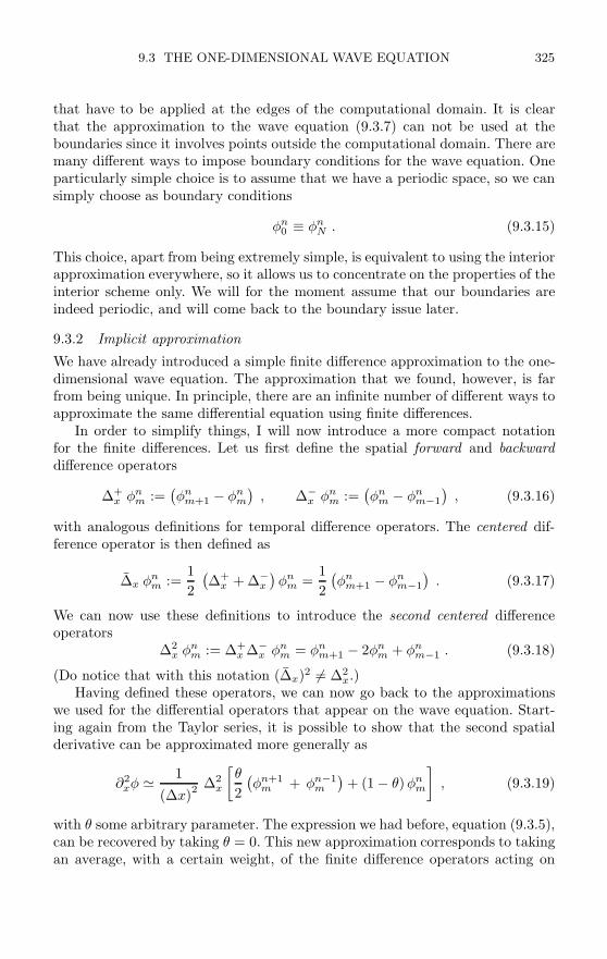
9.3 THE ONE-DIMENSIONAL WAVE EQUATION 325
that have to be applied at the edges of the computational domain. It is clearthat the approximation to the wave equation (9.3.7) can not be used at theboundaries since it involves points outside the computational domain. There aremany different ways to impose boundary conditions for the wave equation. Oneparticularly simple choice is to assume that we have a periodic space, so we cansimply choose as boundary conditions
φn0 ≡ φn
N . (9.3.15)
This choice, apart from being extremely simple, is equivalent to using the interiorapproximation everywhere, so it allows us to concentrate on the properties of theinterior scheme only. We will for the moment assume that our boundaries areindeed periodic, and will come back to the boundary issue later.
9.3.2 Implicit approximation
We have already introduced a simple finite difference approximation to the one-dimensional wave equation. The approximation that we found, however, is farfrom being unique. In principle, there are an infinite number of different ways toapproximate the same differential equation using finite differences.
In order to simplify things, I will now introduce a more compact notationfor the finite differences. Let us first define the spatial forward and backwarddifference operators
∆+x φn
m :=(φn
m+1 − φnm
), ∆−
x φnm :=
(φn
m − φnm−1
), (9.3.16)
with analogous definitions for temporal difference operators. The centered dif-ference operator is then defined as
∆x φnm :=
12(∆+
x + ∆−x
)φn
m =12(φn
m+1 − φnm−1
). (9.3.17)
We can now use these definitions to introduce the second centered differenceoperators
∆2x φn
m := ∆+x ∆−
x φnm = φn
m+1 − 2φnm + φn
m−1 . (9.3.18)
(Do notice that with this notation (∆x)2 = ∆2x.)
Having defined these operators, we can now go back to the approximationswe used for the differential operators that appear on the wave equation. Start-ing again from the Taylor series, it is possible to show that the second spatialderivative can be approximated more generally as
∂2xφ 1(∆x)2
∆2x
[θ
2(φn+1
m + φn−1m
)+ (1 − θ)φn
m
], (9.3.19)
with θ some arbitrary parameter. The expression we had before, equation (9.3.5),can be recovered by taking θ = 0. This new approximation corresponds to takingan average, with a certain weight, of the finite difference operators acting on
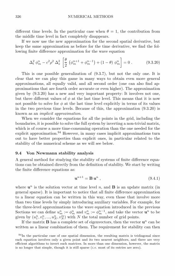
326 NUMERICAL METHODS
different time levels. In the particular case when θ = 1, the contribution fromthe middle time level in fact completely disappears.
If we now use the new approximation for the second spatial derivative, butkeep the same approximation as before for the time derivative, we find the fol-lowing finite difference approximation for the wave equation
∆2t φn
m − c2ρ2 ∆2x
[θ
2(φn+1
m + φn−1m
)+ (1 − θ) φn
m
]= 0 . (9.3.20)
This is one possible generalization of (9.3.7), but not the only one. It isclear that we can play this game in many ways to obtain even more generalapproximations, all equally valid, and all second order (one can also find ap-proximations that are fourth order accurate or even higher). The approximationgiven by (9.3.20) has a new and very important property: It involves not one,but three different values of φ at the last time level. This means that it is nownot possible to solve for φ at the last time level explicitly in terms of its valuesin the two previous time levels. Because of this, the approximation (9.3.20) isknown as an implicit approximation.
When we consider the equations for all the points in the grid, including theboundaries, it is possible to solve the full system by inverting a non-trivial matrix,which is of course a more time-consuming operation than the one needed for theexplicit approximation.94 However, in many cases implicit approximations turnout to have better properties than explicit ones, in particular related to thestability of the numerical scheme as we will see below.
9.4 Von Newmann stability analysis
A general method for studying the stability of systems of finite difference equa-tions can be obtained directly from the definition of stability. We start by writingthe finite difference equations as:
un+1 = B un , (9.4.1)
where un is the solution vector at time level n, and B is an update matrix (ingeneral sparse). It is important to notice that all finite difference approximationto a linear equation can be written in this way, even those that involve morethan two time levels by simply introducing auxiliary variables. For example, forthe three-level approximations to the wave equation introduced in the previousSections we can define un
m := φnm and vn
m := φn−1m , and take the vector un to be
given by (un1 , v
n1 , ..., un
N , vmN ) with N the total number of grid points.
If the matrix B has a complete set of eigenvectors, then the vector un can bewritten as a linear combination of them. The requirement for stability can then
94In the particular case of one spatial dimension, the resulting matrix is tridiagonal sinceeach equation involves only a given point and its two nearest neighbors, and there are veryefficient algorithms to invert such matrices. In more than one dimension, however, the matrixis no longer that simple, though it is still sparse (i.e. most of its entries are zero).

9.4 VON NEWMANN STABILITY ANALYSIS 327
be reduced to asking for the matrix B not to amplify any of its eigenvectors,that is, we must ask for the magnitude of its largest eigenvalue of B, known asits spectral radius, to be less than or equal to 1.
The stability analysis based on the idea just described is quite general, but itrequires a knowledge of the entries of B over all space, including the boundary.There is, however, a very popular stability analysis method that, even though itcan only be shown to give necessary conditions for stability, in many cases turnsout to also give sufficient conditions. This method, originally introduced by vonNewmann, is based on a Fourier decomposition.
To introduce von Newmann’s method, we start by expanding the solutionof (9.4.1) as a Fourier series
un (x) =∑k
un (k) ei k·x , (9.4.2)
where the sum is over all wave vectors k that can be represented on the grid.95
If we now substitute this into the original equation (9.4.1) we find
un+1 = B un , (9.4.3)
where now B is the Fourier transform of the original matrix B, also known asthe amplification matrix. The stability condition now corresponds to asking thatno Fourier mode should be amplified, that is, for the spectral radius of B to beless than or equal to 1. This is von Newmann’s stability condition.
It is important to stress the fact that in order to use this stability criteriawe have assumed two things: 1) The boundary conditions are periodic, sinceotherwise we can not make a Fourier expansion, and 2) the entries of the matrixB are constant (i.e. independent of position), since otherwise it is not possibleto decouple the different Fourier modes.
As an example of von Newmann’s stability analysis we can now study the sta-bility of the implicit approximation to the wave equation we derived previously,equation (9.3.20). Consider a Fourier mode of the form
φnm = ξneimk∆x . (9.4.4)
If we substitute this back into the finite difference equation we find, after somealgebra, a quadratic equation for ξ of the form
Aξ2 + Bξ + C = 0 , (9.4.5)
with coefficients given by
95The shortest wavelength that can be represented on the grid is clearly 2∆x, also knownas the Nyquist limit. This implies that the maximum value that any component of the wavevector can take is π/∆x.
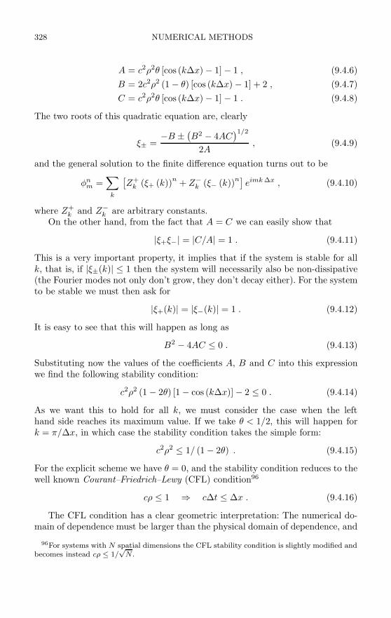
328 NUMERICAL METHODS
A = c2ρ2θ [cos (k∆x) − 1] − 1 , (9.4.6)B = 2c2ρ2 (1 − θ) [cos (k∆x) − 1] + 2 , (9.4.7)C = c2ρ2θ [cos (k∆x) − 1] − 1 . (9.4.8)
The two roots of this quadratic equation are, clearly
ξ± =−B ± (B2 − 4AC
)1/22A
, (9.4.9)
and the general solution to the finite difference equation turns out to be
φnm =
∑k
[Z+k (ξ+ (k))n + Z−
k (ξ− (k))n]eimk∆x , (9.4.10)
where Z+k and Z−k are arbitrary constants.
On the other hand, from the fact that A = C we can easily show that
|ξ+ξ−| = |C/A| = 1 . (9.4.11)
This is a very important property, it implies that if the system is stable for allk, that is, if |ξ±(k)| ≤ 1 then the system will necessarily also be non-dissipative(the Fourier modes not only don’t grow, they don’t decay either). For the systemto be stable we must then ask for
|ξ+(k)| = |ξ−(k)| = 1 . (9.4.12)
It is easy to see that this will happen as long as
B2 − 4AC ≤ 0 . (9.4.13)
Substituting now the values of the coefficients A, B and C into this expressionwe find the following stability condition:
c2ρ2 (1 − 2θ) [1 − cos (k∆x)] − 2 ≤ 0 . (9.4.14)
As we want this to hold for all k, we must consider the case when the lefthand side reaches its maximum value. If we take θ < 1/2, this will happen fork = π/∆x, in which case the stability condition takes the simple form:
c2ρ2 ≤ 1/ (1 − 2θ) . (9.4.15)
For the explicit scheme we have θ = 0, and the stability condition reduces to thewell known Courant–Friedrich–Lewy (CFL) condition96
cρ ≤ 1 ⇒ c∆t ≤ ∆x . (9.4.16)
The CFL condition has a clear geometric interpretation: The numerical do-main of dependence must be larger than the physical domain of dependence, and
96For systems with N spatial dimensions the CFL stability condition is slightly modified andbecomes instead cρ ≤ 1/
√N .

9.5 DISSIPATION AND DISPERSION 329
c t < x stable
c t > x unstable
Fig. 9.2: CFL stability condition. For c∆t ≤ ∆x, the numerical domain of dependenceis larger than the physical domain of dependence (shaded region), and the system isstable. For c∆t > ∆x we have the opposite situation, and the system is unstable.
not the other way around (see Figure 9.2). If this weren’t the case, it would beimpossible for the numerical solution to converge to the exact solution, since asthe grid is refined there will always be relevant physical information that wouldremain outside the numerical domain of dependence. And, as we have seen, theLax theorem implies that if there is no convergence then the system is unstable.
The argument we have just given clearly only applies to explicit schemes.This is because for an implicit scheme, the numerical domain of dependence isin fact the whole grid. In that case there is no simple geometric argument thatcan tell us what the stability condition should be.
In order to obtain the stability condition (9.4.15) we assumed that θ < 1/2.If, on the other hand, we take θ ≥ 1/2 then we must go back to the generalcondition (9.4.14). However, in this case it is easy to see that the condition isalways satisfied. This means that an implicit scheme with θ ≥ 1/2 is stable forall values of ρ, that is, it is unconditionally stable.
This takes us to one of the most important lessons of the theory of finitedifferencing: Simple schemes not always have the best stability properties.97
9.5 Dissipation and dispersion
The idea of decomposing the solution of our finite difference approximation ina Fourier series is not only useful to determine the stability of a scheme. It alsogives us the opportunity to study other related properties of the solutions. Letus concentrate our attention on the case of one spatial dimension, and assumethat we have a linear differential equation that admits solutions of the form
φ (x, t) = e−iωt eikx , (9.5.1)
where for every real wave number k there exists a complex frequency ω given by
97This is even more so for systems of equations of parabolic type (such as the heat equation),for which explicit schemes are practically useless since the stability condition becomes ∆t ∆x2. The problem with this is that it means that if we reduce ∆x by half, we must reduce∆t by a factor of four, so integrating to a desired finite time T quickly becomes prohibitive interms of computer time.

330 NUMERICAL METHODS
ω = ω (k) . (9.5.2)
The explicit form of this relation will of course be determined by the propertiesof our original differential equation. Clearly, the imaginary part of ω will givethe rate of growth or decay of a given Fourier mode with time. A differentialequation that admits solutions for which the imaginary part of ω is negative iscalled a dissipative equation.
It is also useful to define the concept of dispersion: A differential equationis said to be non-dispersive if the real part of ω is a linear function of k, anddispersive otherwise. For this reason, equation (9.5.2) is known as the dispersionrelation.
The wave equation is one example of a differential equation that admits solu-tions of the form (9.5.1). In this case the dispersion relation is simply ω = ±ck,which implies that the wave equation is both non-dissipative and non-dispersive.
The dispersion relation contains within itself very important informationabout the behavior of the solution of a given differential equation. Consider, forexample, a non-dissipative differential equation. Equation (9.5.1) implies that wewill have solutions in the form of traveling sinusoidal waves. The speed of eachwave will be given in terms of its wave number k and its frequency ω by theso-called phase velocity vp(k) defined as
vp(k) :=ω
k. (9.5.3)
In practice, however, we never deal with infinite plane waves but rather withlocalized wave packets. A wave packet that has a narrow Fourier transform,centered at a wavenumber k, doesn’t travel with the phase velocity v(k), butrather with a speed given by:
vg(k) =dω
dk, (9.5.4)
and known as the group velocity. Non-dispersive systems like the wave equationhave the property that the phase velocity and group velocity are equal for allmodes, vp(k) = vg(k).
Even when we are dealing with a differential equation that is both non-dissipative and non-dispersive, it turns out that quite generally these propertiesare not preserved when we consider a finite difference approximation. These ap-proximations are almost always dispersive, and are often also dissipative (noticethat an instability can be interpreted as the result of negative dissipation).
The finite difference approximations to the simple one-dimensional waveequation discussed in the previous sections provide an excellent example of thistype of phenomenon. Let us again consider the general implicit approximationto the 1D wave equation (equation (9.3.20)). Comparing equation (9.5.1) withthe Fourier mode decomposition (9.4.4) used for the von Newmann stability,
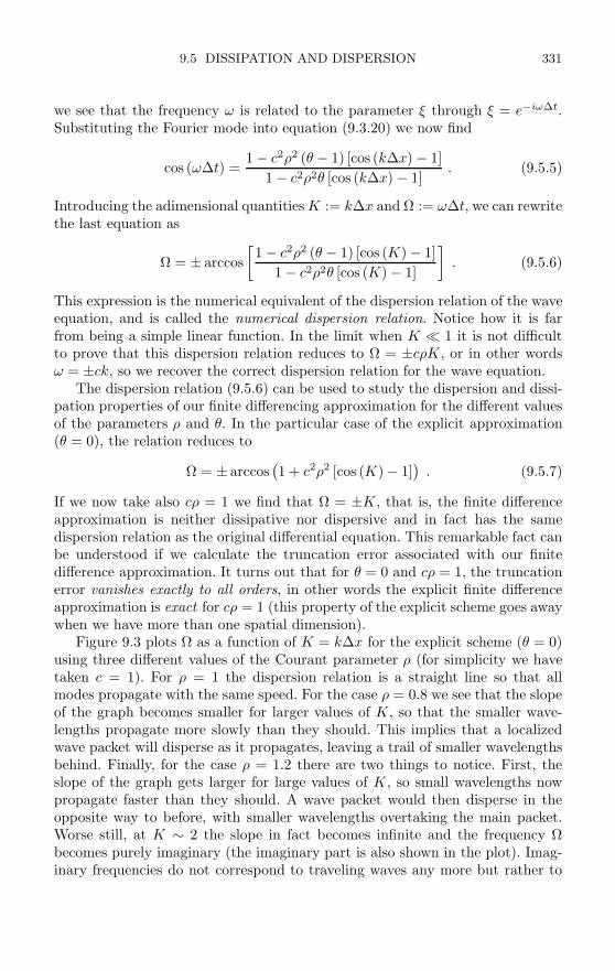
9.5 DISSIPATION AND DISPERSION 331
we see that the frequency ω is related to the parameter ξ through ξ = e−iω∆t.Substituting the Fourier mode into equation (9.3.20) we now find
cos (ω∆t) =1 − c2ρ2 (θ − 1) [cos (k∆x) − 1]
1 − c2ρ2θ [cos (k∆x) − 1]. (9.5.5)
Introducing the adimensional quantities K := k∆x and Ω := ω∆t, we can rewritethe last equation as
Ω = ± arccos[1 − c2ρ2 (θ − 1) [cos (K) − 1]
1 − c2ρ2θ [cos (K) − 1]
]. (9.5.6)
This expression is the numerical equivalent of the dispersion relation of the waveequation, and is called the numerical dispersion relation. Notice how it is farfrom being a simple linear function. In the limit when K 1 it is not difficultto prove that this dispersion relation reduces to Ω = ±cρK, or in other wordsω = ±ck, so we recover the correct dispersion relation for the wave equation.
The dispersion relation (9.5.6) can be used to study the dispersion and dissi-pation properties of our finite differencing approximation for the different valuesof the parameters ρ and θ. In the particular case of the explicit approximation(θ = 0), the relation reduces to
Ω = ± arccos(1 + c2ρ2 [cos (K) − 1]
). (9.5.7)
If we now take also cρ = 1 we find that Ω = ±K, that is, the finite differenceapproximation is neither dissipative nor dispersive and in fact has the samedispersion relation as the original differential equation. This remarkable fact canbe understood if we calculate the truncation error associated with our finitedifference approximation. It turns out that for θ = 0 and cρ = 1, the truncationerror vanishes exactly to all orders, in other words the explicit finite differenceapproximation is exact for cρ = 1 (this property of the explicit scheme goes awaywhen we have more than one spatial dimension).
Figure 9.3 plots Ω as a function of K = k∆x for the explicit scheme (θ = 0)using three different values of the Courant parameter ρ (for simplicity we havetaken c = 1). For ρ = 1 the dispersion relation is a straight line so that allmodes propagate with the same speed. For the case ρ = 0.8 we see that the slopeof the graph becomes smaller for larger values of K, so that the smaller wave-lengths propagate more slowly than they should. This implies that a localizedwave packet will disperse as it propagates, leaving a trail of smaller wavelengthsbehind. Finally, for the case ρ = 1.2 there are two things to notice. First, theslope of the graph gets larger for large values of K, so small wavelengths nowpropagate faster than they should. A wave packet would then disperse in theopposite way to before, with smaller wavelengths overtaking the main packet.Worse still, at K ∼ 2 the slope in fact becomes infinite and the frequency Ωbecomes purely imaginary (the imaginary part is also shown in the plot). Imag-inary frequencies do not correspond to traveling waves any more but rather to

332 NUMERICAL METHODS
0
0.5
1
1.5
2
2.5
3
0.5 1 1.5 2 2.5 3
k x
= 1
= 1.2
= 0.8
(imaginary part) = 1.2
Fig. 9.3: Dispersion relation Ω(k∆x) for the explicit scheme (θ = 1), and for threedifferent values of the Courant parameter ρ (taking c = 1).
solutions that grow exponentially with time, i.e. the corresponding modes areunstable, which is to be expected since we are now violating the CFL condition.
9.6 Boundary conditions
In the previous sections I have discussed different finite difference approximationsto the wave equation assuming that we are using periodic boundary conditions.However, it is clear that periodic boundary conditions generally do not corre-spond to what we expect from a realistic physical scenario. In the general case,we would expect to have one of the following situations:
1. The computational domain represents a finite region of space that is de-limited by real physical boundaries where some kind of exact boundaryconditions should be applied.
2. The computational domain represents a finite region of an infinite space.In this situation, the fact that we must necessarily have a finite compu-tational domain implies that we must use some sort of artificial boundarycondition. This condition, however, should allow the waves to leave thecomputational domain as cleanly as possible (there is no “real” boundarythere). Numerical boundary conditions that have this property are gener-ally known as absorbing boundary conditions, since their work is to absorbmost of the energy of the waves that reach the boundaries, reflecting aslittle as possible back into the grid.98
98There is, in fact, a different approach to the problem of representing an infinite spaceusing a finite computational domain. This approach consists of using a “compactification” ofspace, that is, introducing a new coordinate system that maps all of infinite space into a finiteinterval. In this way, the boundary of the finite differencing grid will correspond to physical
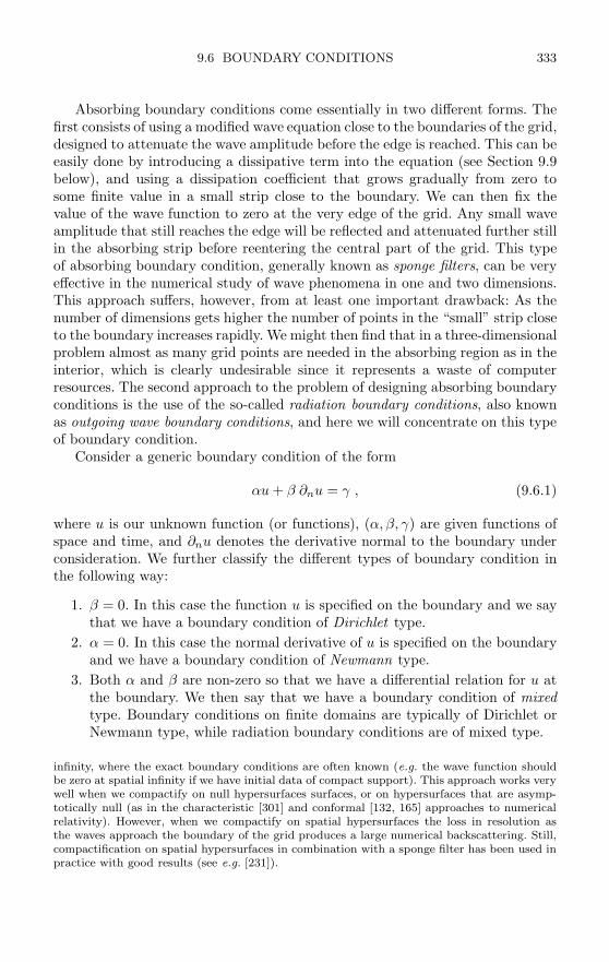
9.6 BOUNDARY CONDITIONS 333
Absorbing boundary conditions come essentially in two different forms. Thefirst consists of using a modified wave equation close to the boundaries of the grid,designed to attenuate the wave amplitude before the edge is reached. This can beeasily done by introducing a dissipative term into the equation (see Section 9.9below), and using a dissipation coefficient that grows gradually from zero tosome finite value in a small strip close to the boundary. We can then fix thevalue of the wave function to zero at the very edge of the grid. Any small waveamplitude that still reaches the edge will be reflected and attenuated further stillin the absorbing strip before reentering the central part of the grid. This typeof absorbing boundary condition, generally known as sponge filters, can be veryeffective in the numerical study of wave phenomena in one and two dimensions.This approach suffers, however, from at least one important drawback: As thenumber of dimensions gets higher the number of points in the “small” strip closeto the boundary increases rapidly. We might then find that in a three-dimensionalproblem almost as many grid points are needed in the absorbing region as in theinterior, which is clearly undesirable since it represents a waste of computerresources. The second approach to the problem of designing absorbing boundaryconditions is the use of the so-called radiation boundary conditions, also knownas outgoing wave boundary conditions, and here we will concentrate on this typeof boundary condition.
Consider a generic boundary condition of the form
αu + β ∂nu = γ , (9.6.1)
where u is our unknown function (or functions), (α, β, γ) are given functions ofspace and time, and ∂nu denotes the derivative normal to the boundary underconsideration. We further classify the different types of boundary condition inthe following way:
1. β = 0. In this case the function u is specified on the boundary and we saythat we have a boundary condition of Dirichlet type.
2. α = 0. In this case the normal derivative of u is specified on the boundaryand we have a boundary condition of Newmann type.
3. Both α and β are non-zero so that we have a differential relation for u atthe boundary. We then say that we have a boundary condition of mixedtype. Boundary conditions on finite domains are typically of Dirichlet orNewmann type, while radiation boundary conditions are of mixed type.
infinity, where the exact boundary conditions are often known (e.g. the wave function shouldbe zero at spatial infinity if we have initial data of compact support). This approach works verywell when we compactify on null hypersurfaces surfaces, or on hypersurfaces that are asymp-totically null (as in the characteristic [301] and conformal [132, 165] approaches to numericalrelativity). However, when we compactify on spatial hypersurfaces the loss in resolution asthe waves approach the boundary of the grid produces a large numerical backscattering. Still,compactification on spatial hypersurfaces in combination with a sponge filter has been used inpractice with good results (see e.g. [231]).
334 NUMERICAL METHODS
As an example of a radiation boundary condition, consider again the case ofthe one-dimensional wave equation. It is easy to see that the appropriate exactradiation boundary conditions are given by
∂tφ − c ∂xφ = 0 , at the left boundary∂tφ + c ∂xφ = 0 , at the right boundary (9.6.2)
These are simple advection equations that represent waves traveling out from thecomputational domain on either side. For initial data of compact support theywill allow the waves to leave the integration region very cleanly without anyreflections. Of course, this is only true if we can apply these boundary conditionsexactly. As soon as we substitute (9.6.2) for some finite difference approximationto it we generally find that outgoing waves are not completely eliminated andsome amount of reflection is always present.
Without loss of generality, let us consider only the condition for the leftboundary. There are many different ways of approximating this condition usingfinite differences. We can consider, for example, a forward difference in both timeand space, resulting in the numerical boundary condition(
φn+10 − φn
0
)− cρ (φn1 − φn
0 ) = 0 , (9.6.3)
where again ρ = ∆t/∆x is the Courant parameter, and where we have assumedthat the numerical grid starts with the grid point m = 0. The approximationabove is clearly explicit, but it is only first order accurate in both space and time(this approximation in fact corresponds to the upwind method for the advectionequation that we will discuss in the next Section). A better approximation tothe radiation boundary condition is obtained by using an implicit approximationfor the spatial derivative, and at the same time introducing an averaged timedifference to approximate the time derivative. Doing this we find[(
φn+10 − φn
0
)+(φn+11 − φn
1
)]− cρ[(
φn+11 − φn+1
0
)+ (φn
1 − φn0 )]
= 0 . (9.6.4)
This approximation is now second order accurate in both space and time. Thefact that it is implicit can seem at first glance to be a drawback, but one mustremember that the boundary condition will be applied once we have alreadyupdated all the interior points. This means that we will already know the valueof φn+1
1 and we can simply solve the above equation for φn+10 :
φn+10 =
11 + cρ
[(cρ − 1)φn+1
1 + (1 + cρ)φn1 + (1 − cρ)φn
0
]. (9.6.5)
In situations where we have more than one spatial dimension, radiationboundary conditions become more complicated. For example, for spherical wavesin three dimensions we typically expect the solution to behave as φ = u(r−ct)/rfor large r. This can be expressed in differential terms as
∂tφ + c ∂rφ + c φ/r = 0 . (9.6.6)
If we are using a Cartesian coordinate system, this equation will usually have tobe applied at the boundaries of a cube, where the normal direction corresponds

9.7 NUMERICAL METHODS FOR FIRST ORDER SYSTEMS 335
to one of the Cartesian directions xi. In that case we can use the fact thatfor a spherically symmetric function, ∂iφ = (xi/r) ∂rφ, and use as a boundarycondition:
xi
r∂tφ + c ∂iφ − cxi
r2φ = 0 . (9.6.7)
This condition can now be applied at each of the Cartesian boundaries by takingxi equal to (x, y, z). Of course, typically our function φ can not be expectedto be spherically symmetric, but if the boundaries are sufficiently far away theangular derivatives will be much smaller than the radial derivative and can besafely ignored without introducing large reflections.
The specific boundary conditions described above only work well for simplesystems like the wave equation. For more complex systems we would need tocarefully consider what are the appropriate boundary conditions at the differ-ential level, which will of course be determined by the type of problem beingsolved. For example, for hyperbolic systems of equations we should first decom-pose the solution into ingoing and outgoing modes at the boundary, and applyboundary conditions only to ingoing modes because applying them to outgoingmodes would violate causality. Only after we have found adequate (and well-posed) boundary conditions at the differential level can we start constructingfinite difference approximations to them.
9.7 Numerical methods for first order systems
In the previous Sections we have introduced the basic concepts behind finite dif-ferencing approximations, using as an example the one-dimensional wave equa-tion. However, the systems of evolution equations that we are mainly interestedin for numerical relativity are typically written as either mixed first order in timeand second order in space systems like the ADM or BSSNOK equations, or fullyfirst order systems like the Euler equations of hydrodynamics. Because of this wewill review here some of the standard numerical methods used for this type ofsystem. We will start by considering numerical methods for the one-dimensionaladvection equation
∂tu + v ∂xu = 0 , (9.7.1)
where u is the wave function and v some constant wave speed. For the finitedifferencing approximation to this equation we take the standard discretizationof spacetime: xm = m∆x, tn = n∆t, un
m = u(tn, xm), with n and m integers.The most obvious method for solving the advection equation numerically is toapproximate ∂tu by a forward time difference, and ∂xu by a centered spacedifference:
un+1m − un
m
∆t+ v
unm+1 − un
m−12∆x
= 0 . (9.7.2)
Solving for un+1m we then find
336 NUMERICAL METHODS
un+1m = un
m − vρ
2(un
m+1 − unm−1
), (9.7.3)
where again ρ stands for the Courant parameter ρ = ∆t/∆x. This approxima-tion is known as the forward Euler method (also called FTCS for forward timecentered space). This method has one very serious drawback: A von Newmannstability analysis shows that the method is unconditionally unstable, i.e. it isunstable for any choice of ∆x and ∆t, so it is useless in practice.
A stable method is obtained by using a backward time difference instead:
un+1m = un
m − vρ
2(un+1
m+1 − un+1m−1
). (9.7.4)
This method, known as backward Euler, is stable but clearly implicit. Both Eu-ler methods are also only first order accurate because of the off-centered timedifferences.
Remarkably, the stability problem with the standard Euler method can befixed if instead of un
m we take the average (unm+1 + un
m−1)/2 in the first term ofequation (9.7.3):
un+1m =
12(un
m+1 + unm−1
)− vρ
2(un
m+1 − unm−1
). (9.7.5)
This method is known as Lax–Friedrichs, and although it is still only first orderaccurate, it is explicit and stable provided the CFL condition vρ ≤ 1 is satisfied.This is another example of how finite difference is sometimes an art as much asa science.
Other more sophisticated methods can be obtained from a Taylor series ex-pansion of the form
u(t + ∆t, x) = u(t, x) + ∆t ∂tu +(∆t)2
2∂2t u + · · ·
= u(t, x) − v∆t ∂xu + v2(∆t)2
2∂2xu + · · · , (9.7.6)
where in the second line we have used the original advection equation to ex-change time derivatives for spatial derivatives. Approximating now the spatialderivatives using centered differences we obtain the so-called Lax–Wendroff finitedifference approximation
un+1m = un
m − vρ
2(un
m+1 − unm−1
)+
v2ρ2
2(un
m+1 − 2unm + un
m−1)
. (9.7.7)
Because of the Taylor expansion, the Lax–Wendroff method is second order ac-curate in both time and space. It is also clearly explicit and turns out to bestable if the CFL condition is satisfied.
The improved stability of Lax–Wendroff can in fact be intuitively understood.First, notice that Lax–Wendroff is basically the forward Euler method plus a

9.7 NUMERICAL METHODS FOR FIRST ORDER SYSTEMS 337
correction term. This correction term is proportional to the second derivative ofu, so we can see the method as a finite difference approximation to the equation
∂tu + v ∂xu =v2∆t
2∂2xu . (9.7.8)
But this is nothing more than the advection-diffusion equation. That is, Lax–Wendroff adds a diffusion (i.e. dissipative) term as a correction to forward Euler,improving its stability properties. The diffusion term vanishes in the continuumlimit, so in the end we will still converge to the solution of the non-diffusiveadvection equation. A similar argument shows that the first order Lax–Friedrichsmethod also adds a diffusive correction term to forward Euler, only in this casewe are in fact adding
[(∆x)2/2∆t
]∂2xu.
There are still other quite standard finite difference approximations to theadvection equation. For example, instead of centered spatial differences we canuse one-sided spatial differences. However, when doing this we must be carefulto use one-sided differences that respect the causal flow of information in orderto obtain a stable system. This leads to the so-called upwind method that takesthe following form
The name of the method comes from the fact that, in order to have stability,we must take finite differences along the direction of the flow. Upwind is againstable as long as the CFL condition is satisfied. It is also only first order accuratein both space and time. Nevertheless, it is at the heart of the modern shockcapturing methods we will discuss in Section 9.10.
un+1m = un
m − vρ(un
m − unm−1
)v ≥ 0 ,
un+1m = un
m − vρ(un
m+1 − unm
)v ≤ 0 .
(9.7.9)
Another quite common method is based on the idea of using centered differ-ences in both space and time. This results in the following method:
un+1m = un−1
m − vρ(un
m+1 − unm−1
). (9.7.10)
There are several things to notice about this method. First, in contrast to allother methods presented so far this is a three-level method. This method isknown as leapfrog, as at each iteration we are using the centered time differenceto “jump” over the middle time level. Leapfrog is second order accurate in bothspace and time, and stable if the CFL condition is satisfied. It can also be easilygeneralized to non-linear equations (which is not the case for Lax–Wendroff, forexample). Still, it has two main drawbacks: First, since it is a three-level method,in order to start it we need to know the solution on the first two time levels. Butfor first order systems the initial data can only give us the very first time leveland nothing more, so that leapfrog needs to be initialized using one of the othermethods for at least one time step. Also, because of the way it is constructed itis not difficult to convince oneself that leapfrog in fact produces an evolution ontwo distinct, and decoupled, numerical grids, one of them taking even values of

338 NUMERICAL METHODS
t
x
n
n–1
n+1
m m+2m+1m–1m–2
Fig. 9.4: Structure of the numerical grid for the leapfrog scheme. Notice how the pointsrepresented by the circles are decoupled from those represented by the stars, so in factwe have two distinct grids.
m for even values of n and odd values of m for odd values of n, and the otherone doing the opposite (see Figure 9.4). This decoupling of the grid can lead tothe development of numerical errors that have a checker board pattern in spaceand time typically known as red-black errors.
Finally, we will introduce one more implicit finite difference approximationto the advection equation. For this we simply take the average of the forwardand backward Euler methods:
un+1m = un
m − vρ
4[(
unm+1 − un
m−1)
+(un+1
m+1 − un+1m−1
)]. (9.7.11)
This approximation is known as the Crank–Nicholson scheme. It turns out tobe second order accurate in both time and space and stable for all values of ρ(i.e it is unconditionally stable). It also forms the basis for a method that hasbecome very common in numerical relativity in the past few years and that wewill discuss in the next Section.
Figure 9.5 shows a schematic representation of the different finite differenceschemes introduced so far using the concept of computational stencil or molecule,i.e. a diagram that shows the relationship between the different grid points usedin the approximation.
Up to this point we have considered only the simple scalar advection equa-tion. However, the methods discussed above can be easily generalized to linearhyperbolic systems of the form
∂tu + A ∂xu = 0 , (9.7.12)
where now u denotes a set of unknowns u = (u1, u2, ...), and A is some matrixwith constant coefficients (the characteristic matrix). Most of the methods dis-cussed above can be used directly by simply replacing the scalar function u withthe vector of unknowns and the speed v with the characteristic matrix A. TheCFL condition now takes the form
max |λa| ∆t ≤ ∆x , (9.7.13)
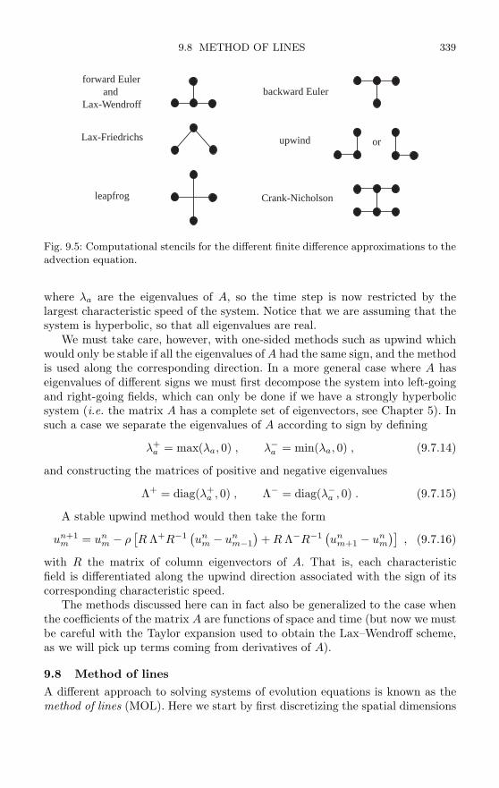
9.8 METHOD OF LINES 339
forward Euler andLax-Wendroff
Crank-Nicholsonleapfrog
upwind or
backward Euler
Lax-Friedrichs
Fig. 9.5: Computational stencils for the different finite difference approximations to theadvection equation.
where λa are the eigenvalues of A, so the time step is now restricted by thelargest characteristic speed of the system. Notice that we are assuming that thesystem is hyperbolic, so that all eigenvalues are real.
We must take care, however, with one-sided methods such as upwind whichwould only be stable if all the eigenvalues of A had the same sign, and the methodis used along the corresponding direction. In a more general case where A haseigenvalues of different signs we must first decompose the system into left-goingand right-going fields, which can only be done if we have a strongly hyperbolicsystem (i.e. the matrix A has a complete set of eigenvectors, see Chapter 5). Insuch a case we separate the eigenvalues of A according to sign by defining
λ+a = max(λa, 0) , λ−a = min(λa, 0) , (9.7.14)
and constructing the matrices of positive and negative eigenvalues
Λ+ = diag(λ+a , 0) , Λ− = diag(λ−a , 0) . (9.7.15)
A stable upwind method would then take the form
un+1m = un
m − ρ[R Λ+R−1 (un
m − unm−1
)+ R Λ−R−1 (un
m+1 − unm
)], (9.7.16)
with R the matrix of column eigenvectors of A. That is, each characteristicfield is differentiated along the upwind direction associated with the sign of itscorresponding characteristic speed.
The methods discussed here can in fact also be generalized to the case whenthe coefficients of the matrix A are functions of space and time (but now we mustbe careful with the Taylor expansion used to obtain the Lax–Wendroff scheme,as we will pick up terms coming from derivatives of A).
9.8 Method of linesA different approach to solving systems of evolution equations is known as themethod of lines (MOL). Here we start by first discretizing the spatial dimensions
340 NUMERICAL METHODS
while leaving the time dimension continuous. For concreteness, let us assumethat we have a single scalar partial differential equation of the form
∂tu = S(u) , (9.8.1)
with S some spatial differential operator. If we use standard finite differencesfor the spatial derivatives we can rewrite our original differential equation as acoupled system of ordinary differential equations of the form
dudt
= S u , (9.8.2)
where now u is a vector constructed from the values of the function u in thedifferent spatial grid points, and S is a matrix (typically sparse) that couples thedifferent grid points. If the resulting system of ordinary differential equations isstable, we can use any standard numerical technique for solving them and wewill obtain a stable evolution.
The method of lines has the advantage that it decouples the choice of spatialand time differencing, so that we can change the order of the spatial differenc-ing or the time integration method independently of each other. It can also begeneralized in a straightforward way to non-linear systems of equations, whichis not always the case with some of the more standard methods (for exampleLax–Wendroff). Moreover, it makes it quite easy to couple codes developed fordifferent systems of equations, like for example the Euler equations for fluid dy-namics and the 3+1 evolution equations for the spacetime. Because of this, codesbased on the method of lines have become increasingly common in numerical rel-ativity over the past decade.
As a simple example, consider again the advection equation (9.7.1), and as-sume that we discretize the spatial derivatives using centered differences. Wethen arrive at the following system of ordinary differential equations
dum
dt= − v
2∆x(um+1 − um−1) . (9.8.3)
We can now solve these equations using, for example, second order Runge–Kuttawhich for a system of equations of the form
du
dt= S(u) , (9.8.4)
takes the formu∗ = un + ∆t S(un)/2 ,
un+1 = un + ∆t S(u∗) .(9.8.5)
Second order Runge–Kutta can be summarized in the following way: Calculatethe sources in the old time step and use them to advance the solution half a timestep. Use now this intermediate step to recalculate the sources, go back and thenadvance the full time step.
9.8 METHOD OF LINES 341
Using Runge–Kutta we can now rewrite our method for solving the advectionequation as
u∗ = un + ∆t S(un)/2 ,
un+1 = un + ∆t S(u∗) .(9.8.6)
which after some algebra becomes
un+1m = un
m − vρ
2(un
m+1 − unm−1
)+
v2ρ2
8(un
m+2 − 2unm + un
m−2)
, (9.8.7)
where as before ρ = ∆t/∆x. We can call this method MOL-RK2 for short. Ifwe now compare the last expression with the Lax–Wendroff method discussedin the previous Section, equation (9.7.7), we see that it has essentially the samestructure except for the fact that the correction term has now been approximatedusing twice the grid spacing. Unfortunately, a von Newmann stability analysisshows that the MOL-RK2 method just described is unstable for any value of ρ,so it is useless in practice.
A stable method is obtained if we use fourth order Runge–Kutta [180] instead,which corresponds to first recursively calculating the quantities
k1 = S(un) , (9.8.8)k2 = S(un + k1∆t/2) , (9.8.9)k3 = S(un + k2∆t/2) , (9.8.10)k4 = S(un + k3∆t) , (9.8.11)
and then taking
un+1 = un +∆t
6(k1 + 2k2 + 2k3 + k4) . (9.8.12)
Notice that fourth order Runge–Kutta requires four evaluations of the sourcesto advance one time step. We can call the method of lines obtained in this wayMOL-RK4. Since this method gives us fourth order accuracy in time, it is naturalto use it with fourth order spatial differencing as well.
Another very common choice for the time integration in the method of lines isthe iterative Crank–Nicholson (ICN) scheme. The idea behind this method is touse an iterative scheme to approach the solution of the standard implicit Crank–Nicholson scheme described in the last Section (equation (9.7.11)). Viewed as amethod of lines, the iteration can be described as follows
u∗(1) = un + ∆t S(un) , (9.8.13)
u∗(l) = un +∆t
2
[S(un) + S(u∗(l−1))
], l = 2, ..., N, (9.8.14)
un+1 = u∗(N) , (9.8.15)
with N ≥ 2. The method takes one initial forward Euler step, uses this tocalculate an approximation to the source in the next time level, and then iterates

342 NUMERICAL METHODS
using the average of the source in the old time level and the latest approximationto the new time level. It is clear that if the iterations converge in the limitN → ∞, we will recover the implicit Crank–Nicholson scheme:
un+1 − un
∆t=
12[S(un) + S(un+1)
]. (9.8.16)
Assuming that the source function S(u) is a linear operator, the iterativemethod can be written formally as
un+1 = un +N∑
k=1
(∆t)k
2k−1 Sk(un) . (9.8.17)
Also, for linear source functions the iterations can be written in an entirelyequivalent way as
u∗(l) = un +∆t
2S(u∗(l−1)) , l = 1, ..., N − 1, (9.8.18)
un+1 = un + ∆t S(u∗(N−1)) , (9.8.19)
with u∗(l) and u∗(l) related through u∗(l) = (un + u∗(l)). The method now takesa series of half steps and a final full step. Viewed in this way we can see that thecase N = 2 is in fact identical to second order Runge–Kutta. Notice that the twodifferent versions of ICN are only equivalent for linear equations; for non-linearequations this equivalence is lost and since there is no a priori reason to preferone version over the other it is a matter of personal choice which version is usedin a given code.
For linear systems, it is also possible to show that the ICN method has thefollowing important properties [14, 283]:
1. In order to obtain a stable scheme we must take at least three steps, that isN ≥ 3. The case N = 2 is enough to achieve second order accuracy, but itis unstable (it is equivalent to second order Runge–Kutta). Stability in factcomes in pairs in terms of the number of steps: 1 and 2 steps are unstable,3 and 4 are stable, 5 and 6 are unstable, and so on (see e.g. [283]).
2. The iterative scheme itself is only convergent if the standard CFL stabilitycondition is satisfied, otherwise the iterations diverge [14].
These two results taken together imply that there is no reason (at least fromthe point of view of stability) to ever do more than three ICN steps. Three stepsare already second order accurate, and provide us with a scheme that is stableas long as the CFL condition is satisfied.99 Increasing the number of iterationswill not improve the stability properties of the scheme any further. In particular,
99Some authors call the N = 3 method a “two-iteration” ICN scheme, since we do an initialEuler step and then iterate twice. This is identical to the “three-step” scheme discussed here.

9.9 ARTIFICIAL DISSIPATION AND VISCOSITY 343
we will never achieve the unconditional stability properties of the full implicitCrank–Nicholson scheme, since if we violate the CFL condition the iterationswill diverge.
Three-step ICN became a workhorse method in numerical relativity for anumber of years. Recently, however, the demand for higher accuracy has seenICN replaced by fourth order Runge–Kutta with fourth order spatial differencing.Still, for applications that do not require very high accuracy, three-step ICN hasproven to be a very robust method.
9.9 Artificial dissipation and viscosity
When we work with non-linear systems of equations like those of relativity orhydrodynamics, many of the stable numerical methods we have described in theprevious Sections become slightly unstable because of the effects of both coef-ficients that depend on the dynamical variables, and lower order terms. Also,in the particular case of hydrodynamics, shock waves can develop that causestandard numerical algorithms to become very inaccurate owing to the appear-ance of spurious high frequency oscillations, known as Gibbs phenomena, nearthe shock front. In order to solve these problems we can add dissipative termsto the finite difference operators that act as “low pass filters” in the sense thatthey preferentially damp modes with wavelength similar to the grid spacing.Such high frequency modes are already unresolved and are therefore severelyaffected by truncation errors, and they are also frequently the source of the in-stabilities (though not always), so that we are often better off dissipating themaway as otherwise they might become unstable and ruin the simulation. Wehave already seen an example of this when we discussed the stability propertiesof the Lax–Friedrichs and Lax–Wendroff schemes. Adding such dissipative termsto a numerical scheme goes under the name of artificial dissipation or artificialviscosity. Although these two terms are often used interchangeably, here I willuse the name artificial dissipation for the more general idea and will keep thename artificial viscosity for a specific technique for dealing with shock waves inhydrodynamical simulations.
The standard way of adding artificial dissipation to a finite difference approx-imation is known as Kreiss–Oliger dissipation [178]. The basic idea is as follows:Assume that we have a finite difference scheme that can be written as
un+1m = un
m + ∆t S(unm) , (9.9.1)
with S(un) some spatial finite difference operator. Let us now modify this schemeby adding a term of the form
un+1m = un
m + ∆t S(unm) − ε
∆t
∆x(−1)N ∆2N
x (unm) , (9.9.2)
with ε > 0, N ≥ 1 an integer, and where ∆2Nx := (∆+
x ∆−x )N is the 2N cen-
tered difference operator. These ∆2Nx operators appear in the finite difference
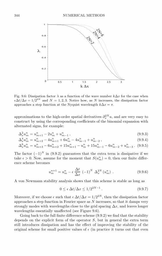
344 NUMERICAL METHODS
0
0.2
0.4
0.6
0.8
1
0.5 1 1.5 2 2.5 3
k x
2=2
2=4
2=6
Fig. 9.6: Dissipation factor λ as a function of the wave number k∆x for the case whenε∆t/∆x = 1/22N and N = 1, 2, 3. Notice how, as N increases, the dissipation factorapproaches a step function at the Nyquist wavelength k∆x = π.
approximations to the high-order spatial derivatives ∂2Nx u, and are very easy toconstruct by using the corresponding coefficients of the binomial expansion withalternated signs, for example:
∆2xun
m = unm+1 − 2un
m + unm−1 , (9.9.3)
∆4xun
m = unm+2 − 4un
m+1 + 6unm − 4un
m−1 + unm−2 , (9.9.4)
∆6xun
m = unm+3 − 6un
m+2 + 15unm+1 − un
m + 15unm−1 − 6un
m−2 + unm−3 . (9.9.5)
The factor (−1)N in (9.9.2) guarantees that the extra term is dissipative if wetake ε > 0. Now, assume for the moment that S(un
m) = 0, then our finite differ-ence scheme becomes
un+1m = un
m − ε∆t
∆x(−1)N ∆2N
x (unm) . (9.9.6)
A von Newmann stability analysis shows that this scheme is stable as long as
0 ≤ ε ∆t/∆x ≤ 1/22N−1 . (9.9.7)
Moreover, if we choose ε such that ε ∆t/∆x = 1/22N , then the dissipation factorapproaches a step function in Fourier space as N increases, so that it damps verystrongly modes with wavelengths close to the grid spacing ∆x, and leaves longerwavelengths essentially unaffected (see Figure 9.6).
Going back to the full finite difference scheme (9.9.2) we find that the stabilitydepends on the explicit form of the operator S, but in general the extra termstill introduces dissipation and has the effect of improving the stability of theoriginal scheme for small positive values of ε (in practice it turns out that even

9.9 ARTIFICIAL DISSIPATION AND VISCOSITY 345
quite small values of ε can result in important improvements in stability). Thebest strategy to improve stability would clearly be to add as much dissipationas possible without either making the scheme unstable (too large ε), or spoilingthe accuracy of the scheme.
The crucial question then becomes: What is the effect of the dissipativeterm on the accuracy of the numerical scheme? In order to see this, let usrewrite (9.9.2) as
un+1m − un
m
∆t= S(un
m) − ε1
∆x(−1)N ∆2N
x (unm) . (9.9.8)
In the limit of small ∆t and ∆x this can be replaced by
∂tu = S(u) − ε (−1)N (∆x)2N−1 ∂2Nx u . (9.9.9)
We then see that we have added a new term to the original differential equationthat vanishes in the continuum limit as (∆x)2N−1. In other words, if the originalnumerical scheme has an accuracy of order m, we would need to use a dissipativeterm such that 2N − 1 ≥ m to be sure that we have not spoiled the accuracyof the scheme. We typically say that the “order” of the dissipative term is givenby the number of derivatives in it, that is 2N , so that if our original schemewas second order accurate we would need to add fourth order dissipation to it(4 − 1 = 3 > 2), and if we had a fourth order scheme we must add sixth orderdissipation (6 − 1 = 5 > 4). Higher order dissipative terms clearly have problemswhen we get very close to the boundaries since we don’t have enough points toapply the dissipative operators. This means that, close to the boundaries, wemust either not use artificial dissipation, or we have to use one-sided dissipativeoperators.
A related, but more specialized, form of artificial dissipation is known asartificial viscosity and is a technique designed to deal with shock waves in hy-drodynamical simulations. The main problem with the Euler equations is thatthe non-linearities give rise to the formation of shocks, i.e. propagating disconti-nuities that arise even from smooth initial data and that are associated with thefact that the characteristic lines cross. Of course, in a realistic physical situationwe do not expect a shock wave to correspond to a true discontinuity, but ratherto a sharp gradient in the hydrodynamical variables. Indeed, if we consider thepresence of viscosity as is done in the Navier–Stokes equations, this is preciselywhat happens. However, in many physical situations, and in most astrophysicalapplications, the viscosity of the fluid is such that the characteristic width of ashock wave is much smaller than the size of the numerical grid, so the shock cannot be resolved numerically. In such cases the numerical methods cause largespurious oscillations to appear close to the shock (Gibbs phenomena), and theseoscillations can seriously affect the accuracy and stability of our finite difference

346 NUMERICAL METHODS
approximation.100 One way to fix this problem is to add by hand an artificialdissipation term that will smooth out the shock into a few grid zones.
There are several important considerations to be made when adding dissipa-tive terms to the Euler equations. In the first place, if we just add a dissipationterm with a constant coefficient we will be affecting the numerical solution every-where. It would clearly be much better to use a dissipation term that will becomelarger in a zone where a shock is likely to develop, and smaller (or even zero) inother regions. Also, if we wish to mimic the physical situation in a realistic way,we need to make sure that the kinetic energy lost because of the presence of thedissipative term does not just vanish from the system, but is in fact convertedinto internal energy.
The original formulation of artificial viscosity is due to von Newmann andRichtmyer [220], and involves modifying the Euler equations by adding an extraviscous contribution Π to the pressure, such that
p → p + Π . (9.9.10)
This already guarantees that energy conservation will be maintained as the vis-cous term will transform kinetic energy into internal energy. In the original workof von Newmann and Richtmyer, the artificial viscosity term was taken to be ofthe form
Π1 = c1ρ (∆x ∂xv)2 , (9.9.11)
where c1 > 0 is a constant coefficient, ρ is the density of the fluid at a given gridpoint, and v is the flow speed. This form of Π is motivated by considering the lossof kinetic energy when two fluid particles have a completely inelastic collision.A different type of artificial viscosity that vanishes less rapidly for small changesin v, and has the effect of reducing unphysical oscillations behind the shock, hasthe form
Π2 = c2ρ cs∆x |∂xv| , (9.9.12)
with c2 > 0 again a constant coefficient, and where cs is the local speed of sound.A more generic form of artificial viscosity will then consist of adding togetherboth types of terms:
Π = c1ρ (∆x ∂xv)2 + c2ρ cs∆x |∂xv| . (9.9.13)
The values of the constants c1 and c2 are adjusted for each simulation, with c2typically an order of magnitude smaller than c1 (notice that the linear viscosityterm introduces an truncation error of order ∆x, while the error associated withthe quadratic term has order (∆x)2 instead). Also, in order to make sure thatviscosity is only added in regions where shocks are likely to form, the coefficients
100The oscillations associated which such Gibbs phenomena are equivalent to those that arisein the Fourier expansion of a discontinuous function and have the same origin. As the resolutionis increased their wavelength becomes smaller and they appear closer and closer to the shockfront, but their amplitude remains essentially the same.

9.10 HIGH RESOLUTION SCHEMES 347
c1 and c2 are usually taken to be different from zero only for regions where theflow lines are converging, that is ∂xv < 0, and are set to zero otherwise.
The simple form of artificial viscosity just described has been modified overthe years, and considerably more sophisticated versions have been proposed,though the basic idea has remained (see for example the recent textbook byWilson and Mathews [300] for the use of artificial viscosity in relativistic hydro-dynamical simulations). Here, however, we will not go into the details of thosemore advanced artificial viscosity techniques and will refer the interested readerto any standard textbook on computational fluid dynamics.
9.10 High resolution schemesAs already mentioned in the last Section, standard finite difference methods haveproblems when dealing with discontinuous solutions such as those associated withhydrodynamical shock waves. Essentially, first order methods show severe dissi-pation close to a discontinuity, while second order methods introduce dispersioneffects that produce large spurious oscillations (Gibbs phenomena). The rate ofconvergence can also be shown to drop near the discontinuity, to order (∆t)1/2
for first order methods, and order (∆t)2/3 for second order methods.As we have seen, one way of dealing with discontinuous solutions is to add
artificial viscosity to our finite difference methods. Indeed, such an approach isstill quite common. The main disadvantage is that artificial viscosity tends to besomewhat ad hoc and must be tailored to the particular problem under study.Because of this we will consider here a more systematic approach to constructingnumerical methods capable of dealing with discontinuous solutions. The discus-sion here will be very brief; for more details the reader can consult the books byLeVeque [187], and by Gustafsson, Kreiss and Oliger [157].
9.10.1 Conservative methodsAs a simple example of an equation that gives rise to discontinuous solutionsstarting from smooth initial data let us consider again Burger’s equation:
∂tu + u ∂xu = 0 . (9.10.1)
As was already discussed in Chapter 7, this equation is a simple non-lineargeneralization of the advection equation, where the wave speed is now given bythe wave function u itself. Burger’s equation is simple enough so that we cansolve it exactly even for discontinuous initial data (the Riemann problem), andwe find that for u > 0, and initial data such that u has a jump from somelarger value at the left to a smaller value to the right, the discontinuity simplypropagates at a constant speed that is the direct average of the values of u tothe left and right (see Section 7.7 for a more detailed explanation).
Let us now assume that we approximate (9.10.1) using a simple generalizationof the upwind method of the form
un+1m = un
m − ∆t
∆xun
m
(un
m − unm−1
). (9.10.2)
348 NUMERICAL METHODS
This method is good for smooth solutions, and stable as long as u > 0 and∆t/∆x ≤ 1. However, it will not converge to the correct solution of the Rie-mann problem for discontinuous initial data. What we find in practice is thateven though the numerical solution looks qualitatively correct, with a propa-gating discontinuity smoothed out over a few grid points because of numericaldissipation, the discontinuity in fact moves at the wrong speed, and this doesnot improve with resolution.
Fortunately, there is a simple way to solve this problem. We must use anumerical method that is written in conservation form. That is, our numericalmethod must have the form
un+1m = un
m − ∆t
∆x
[F
n+1/2m+1/2 − F
n+1/2m−1/2
], (9.10.3)
with Fn+1/2m+1/2 a function that depends on the values of um and um+1 (plus maybe
a few more nearest neighbors), but that has the same functional form as we movefrom one grid point to the next. The function F is known as the numerical fluxfunction. Equation (9.10.3) can be understood as the numerical analog of theintegral form of the conservation law if we think of un
m not as the value of u(x, t)at a single grid point, but rather as the average over the grid cell.
We will usually obtain numerical methods in conservation form if we startfrom the conservative form of the differential equation. For Burger’s equation wecan start from
∂tu + ∂x
(u2/2
)= 0 , (9.10.4)
which can easily be seen to be equivalent to (9.10.1). This leads to the followingupwind method
un+1m = un
m − ∆t
2∆x
[(un
m)2 − (unm−1)
2]
, (9.10.5)
where we have taken Fn+1/2m+1/2 = (un
m)2/2. With this method we now find thatdiscontinuities propagate at the correct speed.
This brings us to the Lax–Wendroff theorem (1960): For hyperbolic systemsof conservation laws, a numerical approximation written in conservation form,if it converges, will converge to a weak solution of the original system.
9.10.2 Godunov’s method
Godunov’s method [146] is an approach to the finite difference approximationof hyperbolic conservation laws that is designed to work well on discontinuoussolutions. It is based on the idea of updating the value of the function by solvingRiemann problems at each cell interface. In this method, we define a piece-wise constant function un that has the value un
m over a given grid cell (with thecell interfaces located halfway between grid points), and we then solve Riemannproblems at each cell interface (see Figure 9.7). This can be done without prob-lems for times short enough so that the wave fronts from neighboring Riemann
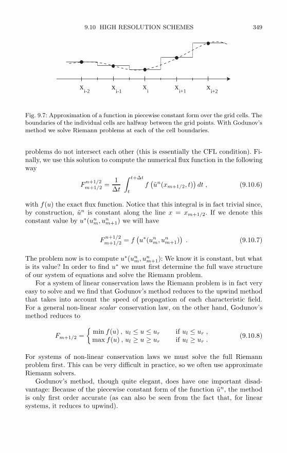
9.10 HIGH RESOLUTION SCHEMES 349
xi-2
xi-1
xi
xi+1
xi+2
Fig. 9.7: Approximation of a function in piecewise constant form over the grid cells. Theboundaries of the individual cells are halfway between the grid points. With Godunov’smethod we solve Riemann problems at each of the cell boundaries.
problems do not intersect each other (this is essentially the CFL condition). Fi-nally, we use this solution to compute the numerical flux function in the followingway
Fn+1/2m+1/2 =
1∆t
∫ t+∆t
t
f(un(xm+1/2, t)
)dt , (9.10.6)
with f(u) the exact flux function. Notice that this integral is in fact trivial since,by construction, un is constant along the line x = xm+1/2. If we denote thisconstant value by u∗(un
m, unm+1) we will have
Fn+1/2m+1/2 = f
(u∗(un
m, unm+1)
). (9.10.7)
The problem now is to compute u∗(unm, un
m+1): We know it is constant, but whatis its value? In order to find u∗ we must first determine the full wave structureof our system of equations and solve the Riemann problem.
For a system of linear conservation laws the Riemann problem is in fact veryeasy to solve and we find that Godunov’s method reduces to the upwind methodthat takes into account the speed of propagation of each characteristic field.For a general non-linear scalar conservation law, on the other hand, Godunov’smethod reduces to
Fm+1/2 =
min f(u) , ul ≤ u ≤ ur if ul ≤ ur ,max f(u) , ul ≥ u ≥ ur if ul ≥ ur .
(9.10.8)
For systems of non-linear conservation laws we must solve the full Riemannproblem first. This can be very difficult in practice, so we often use approximateRiemann solvers.
Godunov’s method, though quite elegant, does have one important disad-vantage: Because of the piecewise constant form of the function un, the methodis only first order accurate (as can also be seen from the fact that, for linearsystems, it reduces to upwind).

350 NUMERICAL METHODS
9.10.3 High resolution methodsFinite difference approximations that are at least second order accurate onsmooth solutions, and give well resolved, non-oscillatory solutions near discon-tinuities, are commonly known as high resolution methods. One natural (thoughnot absolutely necessary) requirement for a high resolution method is that itshould be monotonicity preserving. This means that if the initial data is mono-tonic, then the solution should retain this property for all time. In other words,a monotonicity preserving method would give rise to no spurious oscillations byconstruction.
However, the idea of constructing high resolution, monotonicity preserving,numerical methods is immediately faced with one very serious problem: Godunovhas shown that a linear, monotonicity preserving, finite difference approximationis at most first order accurate. This implies that we must consider non-linearnumerical methods if we want to have a high resolution monotonicity preservingmethod, even for linear systems of equations!
There are two related approaches to constructing non-linear monotonicitypreserving methods that go under the names of flux limiters and slope limiters.Flux limiters use a high order flux FH in smooth regions (e.g. Lax–Wendroff), anda low order flux FL from a monotonic method (e.g. upwind) near a discontinuity.We can then write the full flux F in general as
F = FH − (1 − φ) (FH − FL) , (9.10.9)
where the weight factor φ, known as the limiter, should be close to unity if thedata is smooth, and should approach zero near a discontinuity. The questionis then: How do we measure the smoothness of the data? The most naturalpossibility is to measure this smoothness by comparing the slope of the dynamicalfunction u to the left and right of a given point by defining
θ :=um − um−1um+1 − um
. (9.10.10)
We can then take the limiter φ to be a function of θ.As an example, let us go back to the advection equation (9.7.1) and consider
the Lax–Wendroff method (9.7.7), which for our purposes we will rewrite as
un+1m = un
m − vρ(un
m − unm−1
)− vρ
2(1 − vρ)
(un
m+1 − 2unm + un
m−1), (9.10.11)
with ρ = ∆t/∆x the Courant parameter. Here we have assumed that v > 0,which of course makes no difference for the stability of the Lax–Wendroff method,but does affect the way in which we have chosen to write it since we have clearlyseparated out an “upwind type” first term. We can now rewrite this last methodin flux conservative form and simply read from it the form of the numerical flux.Doing this we find
Fn+1/2m+1/2 = vun
m +v
2(1 − vρ)
(un
m+1 − unm
). (9.10.12)

9.10 HIGH RESOLUTION SCHEMES 351
( )
superbee limiter
minmod limiter
Van Leer's limiter
1 2 3 40
1
2
Fig. 9.8: Different limiter function φ(θ): The solid line corresponds to Sweby’s minmodlimiter, the dashed line to Van Leer’s limiter, and the dotted line to Roe’s superbeelimiter.
The idea now is to change the above flux to
Fn+1/2m+1/2 = vun
m +v
2(1 − vρ)
(un
m+1 − unm
)φ(θ) , (9.10.13)
that is, we have multiplied the second term with the limiter function φ. Noticethat for φ = 1 we recover the Lax–Wendroff flux, while for φ = 0 the expressionreduces to the upwind flux.
How do we choose the form of φ? There are in fact many possibilities thathave been suggested in the literature. For example, Beam and Warming proposetaking φ(θ) = θ, though this is not really a flux limiter and only differs from Lax–Wendroff in the fact that the dissipative term is not centered but is upwindedinstead. Other more interesting limiter functions are the following:
• Sweby’s “minmod” limiter:
φ(θ) = minmod (1, θ) ≡⎧⎨⎩
0 , θ ≤ 0 ,θ , 0 < θ ≤ 1 ,1 , θ ≥ 1 .
(9.10.14)
• Van Leer’s limiter:
φ(θ) =θ + |θ|1 + |θ| . (9.10.15)
• Roe’s “superbee” limiter
φ(θ) = max (0, min(1, 2θ), min(θ, 2)) . (9.10.16)

352 NUMERICAL METHODS
Notice that all three limiters set φ(θ) = 0 for θ < 0, which implies that atextrema the scheme will become only first order accurate. Also, all these limitersare constructed in such a way as to guarantee that the total variation of thenumerical solution, defined as
TV (u) :=∑m
|um − um−1| , (9.10.17)
never increases, i.e. they result in so-called total-variation-diminishing (TVD)schemes. By construction, TVD schemes can not give rise to spurious oscilla-tions since these necessarily would increase the total variation of the function.Because of this, flux limiter methods can resolve discontinuities very sharply.The different limiters result in somewhat different behaviors at discontinuities,with the minmod limiter having more dissipation, the superbee limiter less, andvan Leer’s limiter somewhere in the middle.
Figure 9.8 shows the function φ(θ) for the different limiters. It is in factpossible to show that φ(θ) must lie in the region between the minmod andsuperbee limiters for the resulting scheme to be TVD. As can be seen from thefigure, van Leer’s limiter lies nicely in the middle of this region.
A related, but more geometric, approach to constructing high resolutionmethods is that of slope limiters. The idea here is to generalize Godunov’s methodby replacing the piecewise constant representation by something more accuratesuch as a piecewise linear function (or even a piecewise parabolic). For example,in a given cell we can approximate our function as
u = um + σm(x − xm) , for x ∈ [xm−1/2, xm+1/2
], (9.10.18)
with σm a slope to be determined in terms of the data. For a linear equation theobvious choice for this slope is
σm =um+1 − um
∆x. (9.10.19)
Now, in order to get a second order method we need to calculate the flux at thepoint (xm + ∆x/2, tn + ∆t/2). For the advection equation we will have
Fn+1/2m+1/2 = v u(xm + ∆x/2, tn + ∆t/2)
= vu(xm + (∆x − v∆t)/2, tn)= v (un
m + σnm (1 − vρ)∆x/2)
= vunm +
v
2(1 − vρ)
(un
m+1 − unm
). (9.10.20)
We then see that this choice of σm reduces to Lax–Wendroff, which as we knowis bad for discontinuous solutions.

9.11 CONVERGENCE TESTING 353
A much better choice is to “limit” the value of the slope σm. For example,we can choose the slope as
σm =(
1∆x
)× minmod (um+1 − um, um − um−1)
=(
um+1 − um
∆x
)× minmod (1, θ) , (9.10.21)
which for linear equations is equivalent to the minmod flux limiter. Similarly, wecan use a slope of the form
σm =(
1∆x
)(2 (um+1 − um) (um − um−1)(um+1 − um) + (um − um−1)
)=(
um+1 − um
∆x
)(2θ
1 + θ
), (9.10.22)
for θ > 0, and σm = 0 otherwise, which for linear equations reduces to van Leer’sflux limiter.
There is also a family of limiter methods that relax the TVD condition inorder to increase accuracy near extrema (where TVD methods become onlyfirst order accurate). These higher order methods are known as essentially non-oscillatory (ENO) methods, and instead of asking for the total variation to benon-increasing they allow it to increase as long as its growth is bounded by anexponential that is independent of the initial data. This means that such methodsare total variation stable. However, we will not discuss ENO methods here.
As a final comment, it is important to stress the fact that in the previousdiscussion we have always assumed that the characteristic speed is positive. Thishas entered in the fact that, in order to limit the flux F
n+1/2m+1/2 (or the slope of u in
that region), we have considered the ratio θ = (um − um−1)/(um+1 − um). Thatis, we are considering the differences in the given cell and the cell that is directlyto the left. In the case when the characteristic speed is negative we should haveused instead θ = (um+1 − um)/(um+2 − um+1). More generally, for a stronglyhyperbolic system of equations we need to first diagonalize the system in orderto find the eigenfields and eigenspeeds, and then use one or the other ratio for agiven eigenfunction depending on the sign of its associated eigenspeed. Becauseof this “upwinding”, limiter methods result in considerably more complex codesthan standard methods.
9.11 Convergence testing
Before finishing this Chapter it is important to discuss what is perhaps the mostimportant lesson related to any numerical calculation: A numerical calculationdone at only one resolution (i.e. only one value of ∆x and ∆t) without study-ing how the solution behaves as the resolution is increased is meaningless. We

354 NUMERICAL METHODS
must remember that numerical calculations are approximations to the underly-ing differential equations, and unless we have some idea of the size of the error inthose approximations we have simply no way of knowing if the result of a givennumerical calculation is already close to the correct solution, or if it is simplygarbage.
In order to quantify the error we must carry out what is usually known as aconvergence test. The key idea behind convergence testing is the observation byRichardson [242] that the solution of a stable finite difference approximation canbe interpreted as a continuum function that can be expanded as a power seriesthe discretization parameter ∆
u∆(t, x) = u(t, x) + ∆ e1(t, x) + ∆2e2(t, x) + · · · , (9.11.1)
where u(t, x) is the solution of the original differential equation, and the ei(t, x)are error functions at different orders in ∆. For a first order accurate approxi-mation we expect e1 = 0, for a second order approximation we expect e1 = 0and e2 = 0, etc.
Let us for a moment assume that we know the exact solution to the problem(as in the case of the one-dimensional wave equation). To test the convergenceof our finite difference approximation we perform a calculation at two differentresolutions ∆1 and ∆2, with r ≡ ∆1/∆2 > 1, and calculate the solution error ineach case
ε∆1 = u − u∆1 , ε∆2 = u − u∆2 . (9.11.2)
Notice that in practice this error can only be calculated at the points correspond-ing to the numerical grid under consideration. We then find the r.m.s. norm ofeach solution error and calculate the ratio of both norms
c(t) :=||ε∆1 ||||ε∆2 ||
. (9.11.3)
This ratio is clearly a function of time only, and is known as the convergencefactor (again, it can only be calculated at times when both solution errors aredefined). If we have a finite difference approximation of order n we can now usethe Richardson expansion to find that in the continuum limit the convergencefactor will become
lim∆→0
c(t) =(
∆1
∆2
)n
≡ rn . (9.11.4)
The convergence test is typically done taking r = 2, so that we expect c(t) ∼ 2n.In practice we perform the calculation at several different resolutions and looksat the behavior of c(t) as the resolution increases. If it is close (or getting closer)to the expected value we say that we are in the convergence regime.
Of course, the above procedure will only work if we know the exact solution.This is not true in most cases (after all, if it were true, we would not be usinga numerical approximation), so the best thing that we can hope for is to prove
9.11 CONVERGENCE TESTING 355
that the numerical solution converges to some continuum function.101 In orderto do this we need to use at least three different resolutions ∆1 > ∆2 > ∆3.We then calculate the relative errors between different resolutions and define theconvergence factor as
c(t) :=||u∆1 − u∆2 ||||u∆2 − u∆3 ||
, (9.11.5)
where the differences between solutions must be calculated at the points wherethe grids coincide (alternatively we can interpolate the coarse solution into thefiner grid, but we must remember that interpolation also introduces errors). Inthe continuum limit we then expect the convergence factor to behave as
lim∆→0
c(t) =∆n1 − ∆n
2
∆n2 − ∆n
3
. (9.11.6)
It is usual to take ∆1/∆2 = ∆2/∆3 ≡ r, in which case this again reduces to
lim∆→0
c(t) = rn . (9.11.7)
Because we are taking norms of errors, the convergence test that we have justdescribed is known as a global convergence test. It is also possible to performso-called local convergence tests by simply plotting the relative errors u∆1 −u∆2
and u∆2 −u∆3 directly as functions of position in order to compare them by eye.Since for an order n scheme the Richardson expansion implies that both theseerrors will be proportional to en(t, x), we expect that if the relative errors arerescaled appropriately they should lie approximately one on top of the other.For example, if we have ∆1/∆2 = ∆2/∆3 = r, then after we multiply u∆2 −u∆3
with rn it should coincide (roughly) with u∆1 − u∆2 .Convergence testing not only allows us to verify that the errors are indeed
becoming smaller at the correct rate as the grid is refined, but it also allows usto estimate the remaining solution error. Assume for example that we have anorder n scheme and two numerical calculations with resolutions ∆1 and ∆2, thenthe Richardson expansion implies that
u∆1 − u∆2 = en (∆n1 − ∆n
2 ) + O(∆n+1)= en∆n
2 (rn − 1) + O(∆n+1)∼ ε∆2 (rn − 1) . (9.11.8)
We can then estimate the solution error on our highest resolution grid as
ε∆2 ∼ 1rn − 1
(u∆1 − u∆2) . (9.11.9)
This error estimate is accurate to at least order n+1, and often to order n+2 sincefor centered schemes there are only even powers of n in the Richardson expansion.
101In some cases we in fact do know the exact solution, at least in part. For example, in the3+1 formalism we know that the constraints must vanish, so we can check the convergence ofthe constraints to zero.
356 NUMERICAL METHODS
This allows us to put error bars in a numerical simulation. For example, if wehave a second order accurate scheme and two numerical solutions at differentresolutions with r = ∆1/∆2 = 2, then the solution error on the highest resolutionwill be roughly one-third (22−1 = 3) of the difference between the two numericalsolutions (assuming that we are already in the convergence regime).
As a final comment, the Richardson expansion also allows us to improve ournumerical solution by simply using the results of two or more simulations withdifferent resolutions to estimate the exact solution. For example, once we haveestimated the solution error in our highest resolution we can see that
u = u∆2 − ε∆2 + O(∆n+1) , (9.11.10)
so that
u = u∆2 −1
rn − 1(u∆1 − u∆2) + O(∆n+1) ∼ rnu∆2 − u∆1
rn − 1. (9.11.11)
We then have an estimate of the final solution that is at least one order higherthan our original approximation. This estimate is known as the Richardson ex-trapolation and can improve our solution significantly provided that we startwith an error that is already small.102
I will finish by stressing again the importance of convergence tests in anynumerical calculation: We should simply never believe a numerical calculationfor which no convergence studies have been made.103
102As with any type of extrapolation, Richardson extrapolation is not very good if the initialerror is very large, in which case it might even make things worse. So it should be used withcare.103Boyd goes so far as to define an “idiot” as someone who publishes a numerical calculation
without checking it against an identical calculation with a different resolution [75].

10
EXAMPLES OF NUMERICAL SPACETIMES
10.1 Introduction
In this Chapter we will discuss the application of the techniques of numericalrelativity to some simple spacetimes. We will consider in turn three differenttypes of example, starting from 1+1 “toy” relativity, and moving on to the caseof spherical and axial symmetry. We will discuss some of the special problemsthat arise in each case, such as the issue of gauge shocks in the 1+1 case, and theregularization of the equations in both spherical and axial symmetry, and willalso give examples of numerical simulations of simple physical systems, such asthe evolution of Schwarzschild, the collapse of a scalar field, and the evolutionof a Brill wave spacetime.
10.2 Toy 1+1 relativity
As our first example, let us consider vacuum general relativity in one spatialdimension. It is well known that in such a case the gravitational field is trivialand there are no true dynamics. This is because in a two-dimensional manifoldthe Riemann curvature only has one independent component, namely the Ricciscalar, and this component vanishes in vacuum. However, we can still have non-trivial gauge dynamics that can be used as a simple example of the type ofbehavior we can expect in the higher dimensional case.
In particular, we will be interested in studying the gauge dynamics producedby a slicing condition of the Bonna–Masso family, equation (4.2.52)
∂tα = −α2f(α)K , (10.2.1)
where for simplicity we have taken the shift vector to be zero. Notice that since weonly have one spatial dimension, in this case the trace of the extrinsic curvatureis simply given by K = Kx
x .104
The ADM evolution equations in the 1+1 case, together with the Bona–Massoslicing condition, can be written in first order form as
∂tα = −α2fK , (10.2.2)∂tg = −2αgK , (10.2.3)
and
104This means, in particular, that maximal slicing is trivial since setting K = Kxx = 0 in
vacuum immediately implies α = 1, so that we do not even have gauge dynamics.
357
358 EXAMPLES OF NUMERICAL SPACETIMES
∂tDα + ∂x (αfK) = 0 , (10.2.4)∂tDg + ∂x (2αK) = 0 , (10.2.5)
∂tK + ∂x (αDα/g) = α(K2 − DαDg/2g
), (10.2.6)
where we have defined g := gxx, Dα := ∂x ln α and Dg := ∂x ln g.Before going any further, it is important to notice that the evolution equation
for K can in fact be rewritten as a conservation law in the following way
∂t
(g1/2K
)+ ∂x
(αDα/g1/2
)= 0 . (10.2.7)
If we now define the vector v := (Dα, Dg, K), with K := g1/2K, then the evo-lution equations for the first order variables can be written as a fully conservativesystem of the form
∂tv + ∂x (M v) = 0 , (10.2.8)
with the characteristic matrix M given by:
M =
⎛⎝ 0 0 αf/g1/2
0 0 2α/g1/2
α/g1/2 0 0
⎞⎠ . (10.2.9)
Now, in Chapter 5 it was shown that the ADM evolution equations are notstrongly hyperbolic in the 3+1 case, even when using the Bona–Masso slicingcondition. However, this is no longer true in the case of 1+1 and we find thatthe matrix M defined above has eigenvalues
λ0 = 0 , λ± = ±α (f/g)1/2 , (10.2.10)
with corresponding eigenvectors
e0 = (0, 1, 0) , e± =(f, 2,±f1/2
). (10.2.11)
Since the eigenvalues are clearly real for f > 0, and the two eigenvectors arelinearly independent, the system (10.2.8) is in fact strongly hyperbolic. Theeigenfunctions of the system are defined by (see Chapter 5)
ω = R−1v , (10.2.12)
with R the matrix of column eigenvectors. Using an adequate choice of normal-ization we find that
ω0 = Dα/f − Dg/2 , ω± = K ± Dα/f1/2 , (10.2.13)
which can be easily inverted to give

10.2 TOY 1+1 RELATIVITY 359
K =(ω+ + ω−)
2, (10.2.14)
Dα =f1/2 (ω+ − ω−)
2, (10.2.15)
Dg =(ω+ − ω−)
f1/2− 2ω0 . (10.2.16)
It is important to notice that with the eigenfunctions scaled as above, theirevolution equations also turn out to be conservative and have the simple form
∂tω + ∂x (Λ ω) = 0 , (10.2.17)
with Λ := diag λi. If, however, the eigenfunctions are rescaled in the wayω′
i = Fi(α, g)ωi, then the evolution equations for the ω′i will in general no longer
be conservative, and non-trivial sources will be present. The important point isthat there is in fact one normalization in which the equations are conservative.
10.2.1 Gauge shocksAlthough the 1+1 evolution equations derived above are strongly hyperbolicand therefore well-posed, it turns out that in the general case they can give riseto singular solutions (i.e. gauge pathologies). These singular solutions are verysimilar to the shock waves that develop in hydrodynamics, and because of thisthey are known as gauge shocks [2, 3, 4, 19].
There are at least two different ways in which we can see how gauge shocksdevelop. Let us first consider the evolution equations for the traveling eigenfunc-tions ω±:
∂tω± + ∂x (λ±ω±) = 0 . (10.2.18)
We can rewrite these equations as
∂tω± + λ±∂xω± = −ω±∂xλ± . (10.2.19)
Using now the expressions for λ±, and denoting f ′ ≡ df/dα, we find
∂xλ± = ∓αf1/2
2g3/2∂xg ± f1/2
g1/2
(1 +
αf ′
2f
)∂xα
= λ±
[(f +
αf ′
2
)Dα
f− Dg
2
]= λ±
[(f − 1 +
αf ′
2
)ω+ − ω−
2f1/2+ ω0
], (10.2.20)
and finally
∂tω± + λ±∂xω± =
λ±ω±
[(1 − f − αf ′
2
)ω+ − ω−
2f1/2− ω0
]. (10.2.21)
Assume now that we are in a region such that ω0 = ω− = 0. It is clear thatω0 will not be excited since it does not evolve, nor will ω− be excited since from
360 EXAMPLES OF NUMERICAL SPACETIMES
the equation above we see that all its sources vanish. The evolution equation forω+ then simplifies to
∂tω+ + λ+∂xω+ =λ+
2f1/2
(1 − f − αf ′
2
)ω2+ . (10.2.22)
But this equation implies that ω+ will blow up along its characteristics unlessthe term in parenthesis vanishes:
1 − f − αf ′
2= 0 . (10.2.23)
We will call this the shock avoiding condition. This condition can in fact be easilyintegrated to give
f(α) = 1 + κ/α2 , (10.2.24)
with κ an arbitrary constant. Notice that harmonic slicing corresponds to f = 1which is of this form, but f = const. = 1 is not. Notice also that 1+log slic-ing, for which f = 2/α, though not of the form (10.2.24), nevertheless satisfiescondition (10.2.23) when α = 1 (we will come back to the case of 1+log slicingbelow).
In some cases it is even possible to predict exactly when a blow up willoccur. In order to see this we first need to define the rescaled eigenfunctionsΩ± := αω±/g1/2. For their evolution equations we now find
∂tΩ± + λ±∂xΩ± =(
1 − f − αf ′
2
)Ω2±2
+(
1 − f +αf ′
2
)Ω±Ω∓
2. (10.2.25)
Notice that with this new scaling, all contributions from ω0 to the sources havedisappeared. If we now assume that we have initial data such that Ω− = 0, thenthe evolution equation for Ω+ simplifies to
∂tΩ+ + λ+∂xΩ+ =(
1 − f − αf ′
2
)Ω2+2
, (10.2.26)
which can be rewritten as
dΩ+dt
=(
1 − f − αf ′
2
)Ω2+2
, (10.2.27)
with d/dt the derivative along the characteristic. The last equation has a veryimportant property: For constant f the coefficient of the quadratic source termis itself also constant. In that case the equation can be easily integrated to find(assuming f = 1)
Ω+ =Ω0+
1 − (1 − f) Ω0+ t/2, (10.2.28)
where Ω0+ ≡ Ω+(t = 0). The solution will then blow up at a finite time given byt∗ = 2/[(1 − f) Ω0+]. Clearly, this time will be in the future if (1 − f) Ω0+ > 0,
10.2 TOY 1+1 RELATIVITY 361
otherwise it will be in the past. Since, in general, Ω0+ will not be constant inspace, the first blow-up will occur at the time
t∗ = 2/[(1 − f) max(Ω0+(x))] . (10.2.29)
This shows that blow-ups can easily develop when we use the Bona–Massoslicing condition with a function f(α) such that (10.2.23) does not hold. Ofcourse, this does not imply that such blow-ups will always develop, since theirappearance will clearly depend on the specific form of the initial data being used,but it does show that we should not be terribly surprised if they do.
There is another way in which we can see how these blow-ups develop thatprovides us with a more direct geometrical interpretation of the problem. Con-sider now the evolution of the eigenspeeds themselves along their correspondingcharacteristic lines. From (10.2.10) we find that
∂tλ± = ±∂t
(αf1/2/g1/2
), (10.2.30)
and using the evolution equations for α and g this reduces to
∂tλ± =αλ±g1/2
(1 − f − αf ′
2
)K
=αλ±g1/2
(1 − f − αf ′
2
)(ω+ + ω−)
2. (10.2.31)
In a similar way we find for the spatial derivative
∂xλ± = λ±
[Dα
f
(f +
αf ′
2
)− Dg
2
]= λ±
[(1 − f − αf ′
2
)(ω− − ω+)
2f1/2+ ω0
]. (10.2.32)
The last two equations together imply that
∂tλ± + λ±∂xλ± =αλ±g1/2
[(1 − f − αf ′
2
)ω∓ ± f1/2ω0
]. (10.2.33)
If we now consider again a region where ω− = ω0 = 0, the last equation reducesto
∂tλ+ + λ+∂xλ+ = 0 . (10.2.34)
But this is nothing more than Burgers’ equation, the prototype for studyingshock formation (see Chapter 7). This shows that the blow-ups studied abovecorrespond to places where the characteristic lines cross. At those points thespatial derivative of λ+ becomes infinite, and since this derivative is given interms of eigenfields, some of the eigenfields must blow up. In other words, the
362 EXAMPLES OF NUMERICAL SPACETIMES
blow-ups associated with the Bona–Masso slicing condition develop precisely asshocks do, and it is because of this that we refer to them as gauge shocks.
At this point we could worry about a possible inconsistency in our analysis.The fact that we obtain Burgers’ equation independently of the value of thefunction f(α) would seem to indicate that gauge shocks should develop even ifthe shock avoiding condition (10.2.23) is satisfied. But this not the case sincefrom the derivation above we can easily see that if (10.2.23) is satisfied, andwe are in a region with ω0 = 0, then ∂tλ+ = ∂xλ+ = 0. So Burgers’ equation,though formally still correct, becomes trivial.
A very important question is what happens to the geometry of the spacetimebeing evolved when a gauge shock develops. Since we are simply considering theevolution of a non-trivial foliation of Minkowski spacetime, it is clear that thebackground geometry remains perfectly regular. Therefore, the only thing thatcan become pathological are the spatial hypersurfaces that determine the folia-tion. As the numerical examples of the following Section will show, the formationof a gauge shock indicates that the spatial hypersurface has in fact become non-smooth (it has developed a kink).
10.2.2 Approximate shock avoidance
Before showing some numerical examples of the formation of gauge shocks, let usgo back to the issue of what form of the function f(α) we should use in order toavoid gauge shocks. As already mentioned, the shock avoiding condition (10.2.23)can be trivially integrated and we find that in order to avoid gauge shocks it isnecessary to choose f(α) of the form (10.2.24). In fact, in that expression wemust take κ > 0, to be sure that f remains positive for small values of α, asotherwise the system of evolution equations would stop being hyperbolic.
Now, for κ > 0 and small α we find that f ∼ 1/α2, so from our discussionon singularity avoidance in Chapter 4 we see that the slicing will be stronglysingularity avoiding. However, we can also see that in this case we are in theregime for which the lapse can easily become negative. This means that the so-lution (10.2.24) has a serious drawback for any non-zero value of κ, since it canallow the lapse to become negative as it collapses to zero. This would seem toimply that the requirements of avoiding gauge shocks while at the same timeguaranteeing that the lapse will not become negative are mutually incompati-ble, except in the particular case of harmonic slicing f = 1. On the other hand,harmonic slicing is only marginally singularity avoiding and is therefore not de-sirable when evolving black hole spacetimes (unless we are interested in studyingthe singularity itself).
In order to look for a useful slicing condition we will therefore relax ourrequirements and look for approximate solutions of the shock avoiding condi-tion (10.2.23). We start by assuming that the lapse is very close to 1, that is
α = 1 + ε , (10.2.35)
with ε 1. Notice that the limit above applies to situations that are close to

10.2 TOY 1+1 RELATIVITY 363
flat space, but generally does not apply to strong field regions (like the regionclose to a black hole) where the lapse can be expected to be very different from 1.However, in such regions considerations about singularity avoidance are probablymore important. Our aim is to find slicing conditions that can avoid singularitiesin strong field regions, and at the same time do not have a tendency to generateshocks in weak field regions.
We can now expand f in terms of ε as
f = a0 + a1ε + O(ε2) = a0 + a1(α − 1) + O(ε2) , (10.2.36)
and look for solutions to (10.2.23) to lowest order in ε. Substituting (10.2.36)into (10.2.23) we find
1 − a0 − a1/2 + O(ε) = 0 . (10.2.37)
This means that if we want condition (10.2.23) to be satisfied to lowest order inε we must ask for
a1 = 2 (1 − a0) , (10.2.38)
which implies
f = a0 + 2 (1 − a0) ε + O(ε2)= (3a0 − 2) + 2 (1 − a0)α + O(ε2) . (10.2.39)
Here we must remember that (10.2.39) is just an expansion for small ε. Anyform of the function f(α) that has the same expansion to first order in ε willalso satisfy condition (10.2.23) to lowest order. For example, one family of suchfunctions emerges if we ask for f(α) to have the form
f =p0
1 + q1ε. (10.2.40)
It is not difficult to show that for this to have an expansion of the form (10.2.39)we must ask for
p0 = a0 , q1 = 2 (a0 − 1) /a0 , (10.2.41)
which implies
f =a20
a0 + 2 (a0 − 1) ε=
a20(2 − a0) + 2 (a0 − 1)α
. (10.2.42)
Notice that if we take a0 = 1 we recover harmonic slicing. But there is oneother case that is of special interest: For a0 = 2 the previous solution reduces to
f = 2/α , (10.2.43)
which corresponds to a member of the 1+log family. The crucial observation hereis that, as already mentioned in Chapter 4, this specific member of the 1+logfamily is precisely the one that has been found empirically to be very robust

364 EXAMPLES OF NUMERICAL SPACETIMES
in black hole simulations, and because of this it is considered as the standard1+log slicing. The fact that it is the only member of the 1+log family thatsatisfies condition (10.2.23), even approximately, means that we should expectit to be particularly well behaved.
Notice, however, that standard 1+log slicing avoids gauge shocks only if thelapse function α is close to 1, so we should not be surprised to find that 1+logdevelops gauge shocks when the lapse has collapsed to values close to 0, as istypical in regions close to a black hole. Moreover, the analysis presented hereapplies only to the simple 1+1-dimensional case, and while gauge shocks willcertainly still exist in the higher dimensional case (since after all 1+1 is just aspecial case of 3+1), we could easily expect other potential gauge pathologiesto appear. Nevertheless, empirically it has been found that standard 1+log is(perhaps surprisingly) extremely robust in black hole simulations, and becauseof this it has become the de facto standard slicing condition when studying, forexample, inspiral black hole collisions. Still, there is evidence that, at least insome cases, black hole simulations using a 1+log slicing condition do developgauge problems [141], but whether such problems are gauge shocks in the sensediscussed here (i.e. singularities associated with the crossing of characteristics)or some different type of gauge pathology still remains an open question.
10.2.3 Numerical examples
We will now show some examples of numerical simulations of a 1+1 vacuumspacetime to see how gauge shocks can appear very easily, and how the shockavoiding condition derived in the previous Section does indeed eliminate them.
We start by describing the initial data used in the simulations. Since the argu-ment presented in the previous Section that allows us to predict the precise timeof formation of a gauge shock depends on having only a mode propagating in aspecific direction, we will be interested in constructing initial data correspondingto such a purely traveling mode.
Notice that the simplest way to construct initial data is to just take a trivialinitial slice in Minkowski coordinates, and use a non-trivial initial lapse functionto introduce a later distortion. However, since in this case the initial extrinsiccurvature vanishes, we can see from (10.2.13) that, inevitably, modes travelingin both directions will be excited. We then conclude that in order to have wavespropagating in only one direction we are forced to consider a non-trivial initialslice.
The initial data considered here has already been discussed in [2], and isconstructed as follows: We start by considering an initial slice given in Minkowskicoordinates (tM , xM ) as
tM = h(xM ) , (10.2.44)
with h some profile function that decays rapidly (e.g. a Gaussian function). It isthen not difficult to show that if we keep x = xM as our spatial coordinate, thespatial metric and extrinsic curvature turn out to be
10.2 TOY 1+1 RELATIVITY 365
g = 1 − h′2 ⇒ Dg = −2h′h′′/g , (10.2.45)
Kxx = −h′′/√
g ⇒ K = −h′′/g . (10.2.46)
Assume now that we want to have waves traveling to the right (the oppositesituation can be done in an analogous way). This means that we want ω− = 0,which in turn implies that
Dα =√
f K = −√
f h′′/g . (10.2.47)
This results in the following differential equation for α:
∂xα = −α√
f h′′/(1 − h′2) . (10.2.48)
In the particular case when f is a constant the above equation can be easilyintegrated to find
α =(
1 − h′
1 + h′
)√f/2
. (10.2.49)
From this we can reconstruct the rescaled eigenfunction Ω+, and use equa-tion (10.2.29) to predict the time of shock formation given a specific form ofh(x). In all the simulations shown here, the profile function h has been chosento be a simple Gaussian of the form
h(x) = e−x2/10 . (10.2.50)
But do notice that even if we keep h(x) always the same, changing the value off will change the initial lapse (10.2.49).
The evolution code used for the simulations is based on a method of linesintegration with three-step iterative Crank–Nicholson. For the spatial differenti-ation the code uses a slope limiter method of van Leer’s type (see Chapter 9).No artificial dissipation is introduced. Since the slope limiter method requires
information about the direction of propagation, the code evolves the eigenfields(ω0, ω±) directly, and the variables (Dα, Dg, K) are later reconstructed fromthese.
Consider first an evolution with f = 0.5. Figure 10.1 shows the numericalevolution of the eigenfield ω+ and the lapse function α, using a resolution of∆x = 0.003125 and a Courant factor of ∆t/∆x = 0.5. For the initial data usedhere, according to (10.2.29) a blow-up is expected at time T ∗ 9.98. The plotshows both the initial data (dotted lines) and the numerical solution at timet = 10 (solid lines), just after the expected blow-up. We clearly see how theeigenfield ω+ has developed a large spike at the center of the pulse, while thelapse has developed a corresponding sharp gradient (the numerical solution forω+ does not in fact become infinite because the numerical method has someinherent dissipation). Notice also that after t = 10 the pulse has propagated adistance of ∼ 7, in accordance with the fact that the characteristic speed in thiscase is λ = α
√f/g ∼ √
f ∼ 7.07.

366 EXAMPLES OF NUMERICAL SPACETIMES
1 0 1 2 3 4 5 6 7 8
4 2 0 2 4 6 8 10 12
x
Eigenfield +
0.9
0.95
1
1.05
1.1
4 2 0 2 4 6 8 10 12
x
Lapse function
Fig. 10.1: Evolution of the eigenfield ω+ and the lapse function α for the case wheref = 0.5. The dotted lines show the initial data, and the solid lines the solution att = 10, just after the expected blow-up.
32.5
21.5
10.5 0
0.5 1
5 0 5 10 15 20 25 30
x
Eigenfield +
0.8 0.85
0.9 0.95
1 1.05
1.1 1.15
1.2
5 0 5 10 15 20 25 30
x
Lapse function
Fig. 10.2: Evolution of the eigenfield ω+ and the lapse function α for the case wheref = 1.5. The dotted lines show the initial data, and the solid lines the solution att = 21, just after the expected blow-up.
Next, consider the case where f = 1.5. For the same profile function h(x) asbefore, equation (10.2.29) now predicts a blow-up at time T ∗ = 20.84. Figure 10.2shows the numerical evolution of ω+ and α in this case, using the same resolutionand Courant parameter as before. The plot again shows both the initial data(dotted lines), and the numerical solution at time t = 21 (solid lines), just afterthe expected blow-up. Notice that ω+ has now developed two large spikes at thefront and back of the pulse, with corresponding sharp gradients developing inthe lapse function α. The sign of the spikes in ω+ has also been reversed. Noticealso that in this case the pulse has traveled a distance of ∼ 25 after t = 21,corresponding to a characteristic speed of λ ∼ √
f ∼ 1.22.We then see that for both cases with f = const. = 1, gauge shocks develop as
expected. For completeness, Figure 10.3 shows a simulation of the same initialdata, but now using harmonic slicing corresponding to f = 1. The plot shows
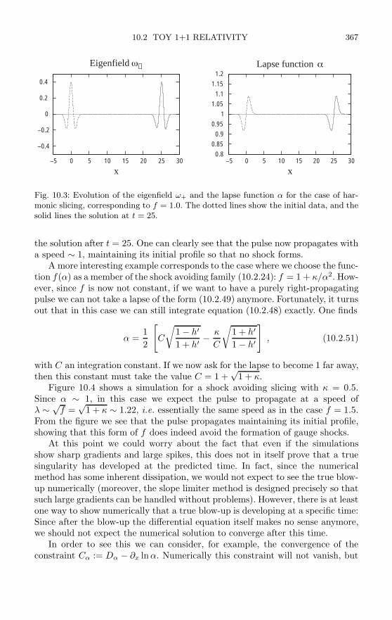
10.2 TOY 1+1 RELATIVITY 367
0.4
0.2
0
0.2
0.4
5 0 5 10 15 20 25 30
x
Eigenfield +
0.8 0.85
0.9 0.95
1 1.05
1.1 1.15
1.2
5 0 5 10 15 20 25 30
x
Lapse function
Fig. 10.3: Evolution of the eigenfield ω+ and the lapse function α for the case of har-monic slicing, corresponding to f = 1.0. The dotted lines show the initial data, and thesolid lines the solution at t = 25.
the solution after t = 25. One can clearly see that the pulse now propagates witha speed ∼ 1, maintaining its initial profile so that no shock forms.
A more interesting example corresponds to the case where we choose the func-tion f(α) as a member of the shock avoiding family (10.2.24): f = 1 + κ/α2. How-ever, since f is now not constant, if we want to have a purely right-propagatingpulse we can not take a lapse of the form (10.2.49) anymore. Fortunately, it turnsout that in this case we can still integrate equation (10.2.48) exactly. One finds
α =12
[C
√1 − h′
1 + h′ −κ
C
√1 + h′
1 − h′
], (10.2.51)
with C an integration constant. If we now ask for the lapse to become 1 far away,then this constant must take the value C = 1 +
√1 + κ.
Figure 10.4 shows a simulation for a shock avoiding slicing with κ = 0.5.Since α ∼ 1, in this case we expect the pulse to propagate at a speed ofλ ∼ √
f =√
1 + κ ∼ 1.22, i.e. essentially the same speed as in the case f = 1.5.From the figure we see that the pulse propagates maintaining its initial profile,showing that this form of f does indeed avoid the formation of gauge shocks.
At this point we could worry about the fact that even if the simulationsshow sharp gradients and large spikes, this does not in itself prove that a truesingularity has developed at the predicted time. In fact, since the numericalmethod has some inherent dissipation, we would not expect to see the true blow-up numerically (moreover, the slope limiter method is designed precisely so thatsuch large gradients can be handled without problems). However, there is at leastone way to show numerically that a true blow-up is developing at a specific time:Since after the blow-up the differential equation itself makes no sense anymore,we should not expect the numerical solution to converge after this time.
In order to see this we can consider, for example, the convergence of theconstraint Cα := Dα − ∂x ln α. Numerically this constraint will not vanish, but
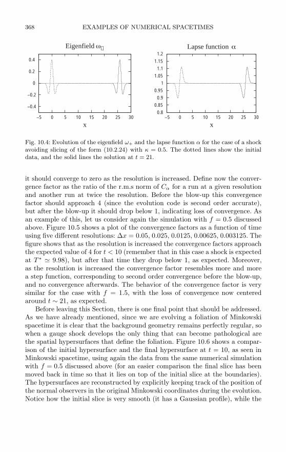
368 EXAMPLES OF NUMERICAL SPACETIMES
0.4
0.2
0
0.2
0.4
5 0 5 10 15 20 25 30
x
Eigenfield +
0.8 0.85
0.9 0.95
1 1.05
1.1 1.15
1.2
5 0 5 10 15 20 25 30
x
Lapse function
Fig. 10.4: Evolution of the eigenfield ω+ and the lapse function α for the case of a shockavoiding slicing of the form (10.2.24) with κ = 0.5. The dotted lines show the initialdata, and the solid lines the solution at t = 21.
it should converge to zero as the resolution is increased. Define now the conver-gence factor as the ratio of the r.m.s norm of Cα for a run at a given resolutionand another run at twice the resolution. Before the blow-up this convergencefactor should approach 4 (since the evolution code is second order accurate),but after the blow-up it should drop below 1, indicating loss of convergence. Asan example of this, let us consider again the simulation with f = 0.5 discussedabove. Figure 10.5 shows a plot of the convergence factors as a function of timeusing five different resolutions: ∆x = 0.05, 0.025, 0.0125, 0.00625, 0.003125. Thefigure shows that as the resolution is increased the convergence factors approachthe expected value of 4 for t < 10 (remember that in this case a shock is expectedat T ∗ 9.98), but after that time they drop below 1, as expected. Moreover,as the resolution is increased the convergence factor resembles more and morea step function, corresponding to second order convergence before the blow-up,and no convergence afterwards. The behavior of the convergence factor is verysimilar for the case with f = 1.5, with the loss of convergence now centeredaround t ∼ 21, as expected.
Before leaving this Section, there is one final point that should be addressed.As we have already mentioned, since we are evolving a foliation of Minkowskispacetime it is clear that the background geometry remains perfectly regular, sowhen a gauge shock develops the only thing that can become pathological arethe spatial hypersurfaces that define the foliation. Figure 10.6 shows a compar-ison of the initial hypersurface and the final hypersurface at t = 10, as seen inMinkowski spacetime, using again the data from the same numerical simulationwith f = 0.5 discussed above (for an easier comparison the final slice has beenmoved back in time so that it lies on top of the initial slice at the boundaries).The hypersurfaces are reconstructed by explicitly keeping track of the position ofthe normal observers in the original Minkowski coordinates during the evolution.Notice how the initial slice is very smooth (it has a Gaussian profile), while the

10.3 SPHERICAL SYMMETRY 369
0
1
2
3
4
5
0 2 4 6 8 10 12t
Convergence factor
Fig. 10.5: Convergence of the constraint Cα for the simulation with f = 0.5 done at thefive different resolutions: ∆x = 0.05, 0.025, 0.0125, 0.00625, 0.003125. As the resolutionincreases, the convergence factors approach the expected value of 4 for t < 10, but afterthat time they drop sharply indicating loss of convergence.
final slice has developed a sharp kink. This shows that the formation of a gaugeshock indicates that the hypersurface, though still spacelike everywhere, is nolonger smooth (its derivative is now discontinuous).
10.3 Spherical symmetry
As our second example we will consider the case of spherically symmetric space-times – a case that, though still relatively simple, nevertheless has many im-portant physical applications. This case is interesting for several reasons. In thefirst place, even though it already represents a full three-dimensional spacetime(as opposed to the 1+1 case studied in the previous sections), the dynamicalvariables depend only on the radial coordinate, so the numerical codes are stillonly one-dimensional. Because of this it is standard in numerical relativity to re-fer codes for spherically symmetric spacetimes as “one-dimensional” (1D) codes.On the other hand, many interesting astrophysical systems, in particular starsand black holes, are spherically symmetric to a very good approximation, so thatspherical symmetry already allows us to study interesting physical problems suchas the stability of stars, gravitational collapse, horizon dynamics, etc. Perhapsthe main drawback of spherical symmetry is the fact that in such a case there areno gravitational waves, so we are missing one key element of general relativity.Still, it was precisely in spherical symmetry that the first major contributionof numerical relativity to the understanding of general relativity was made: thediscovery of critical phenomena in gravitational collapse by Choptuik [98].
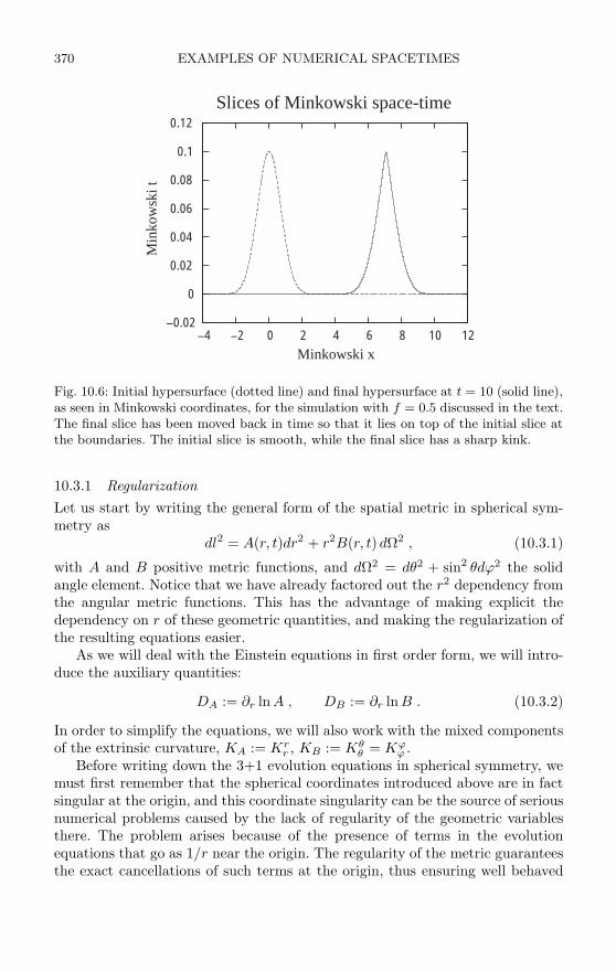
370 EXAMPLES OF NUMERICAL SPACETIMES
0.02
0
0.02
0.04
0.06
0.08
0.1
0.12
4 2 0 2 4 6 8 10 12
Min
kow
ski t
Minkowski x
Slices of Minkowski space-time
Fig. 10.6: Initial hypersurface (dotted line) and final hypersurface at t = 10 (solid line),as seen in Minkowski coordinates, for the simulation with f = 0.5 discussed in the text.The final slice has been moved back in time so that it lies on top of the initial slice atthe boundaries. The initial slice is smooth, while the final slice has a sharp kink.
10.3.1 RegularizationLet us start by writing the general form of the spatial metric in spherical sym-metry as
dl2 = A(r, t)dr2 + r2B(r, t) dΩ2 , (10.3.1)
with A and B positive metric functions, and dΩ2 = dθ2 + sin2 θdϕ2 the solidangle element. Notice that we have already factored out the r2 dependency fromthe angular metric functions. This has the advantage of making explicit thedependency on r of these geometric quantities, and making the regularization ofthe resulting equations easier.
As we will deal with the Einstein equations in first order form, we will intro-duce the auxiliary quantities:
DA := ∂r ln A , DB := ∂r lnB . (10.3.2)
In order to simplify the equations, we will also work with the mixed componentsof the extrinsic curvature, KA := Kr
r , KB := Kθθ = Kϕ
ϕ .Before writing down the 3+1 evolution equations in spherical symmetry, we
must first remember that the spherical coordinates introduced above are in factsingular at the origin, and this coordinate singularity can be the source of seriousnumerical problems caused by the lack of regularity of the geometric variablesthere. The problem arises because of the presence of terms in the evolutionequations that go as 1/r near the origin. The regularity of the metric guaranteesthe exact cancellations of such terms at the origin, thus ensuring well behaved

10.3 SPHERICAL SYMMETRY 371
solutions. This exact cancellation, however, though certainly true for analyticalsolutions, usually fails to hold for numerical solutions. One then finds that the1/r terms do not cancel and the numerical solution becomes ill-behaved nearr = 0: It not only fails to converge at the origin, but it can also easily turn outto be violently unstable after just a few time steps.
The usual way to deal with the regularity problem is to use the so-called areal(or radial) gauge, where the radial coordinate r is chosen in such a way that theproper area of spheres of constant r is always 4πr2 (so that B = 1 during thewhole evolution). If, moreover, we also choose a vanishing shift vector we endup in the so-called polar-areal gauge [48, 97], for which the lapse is forced tosatisfy a certain ordinary differential equation in r. The name polar comes fromthe fact that, for this gauge choice, there is only one non-zero component of theextrinsic curvature tensor, namely Krr [48]. In the polar-areal gauge the problemof achieving the exact cancellation of the 1/r terms is reduced to imposing theboundary condition A = 1 at r = 0, which can be easily done if we solve forA directly from the Hamiltonian constraint (which in this case reduces to anordinary differential equation in r), and ignore its evolution equation. If we dothis in vacuum, we end up inevitably with Minkowski spacetime in the usual co-ordinates (we can also recover Schwarzschild by working in isotropic coordinatesand factoring out the conformal factor analytically).
The main drawback of the standard approach is that the gauge choice hasbeen completely exhausted. In particular, the polar-areal gauge can not penetrateapparent horizons, since inside an apparent horizon it is impossible to keep theareas of spheres fixed without a non-trivial shift vector.105 One would then liketo have a way of dealing with the regularity issue that allows more genericgauge choices to be made. Because of this I will discuss here a more generalregularization procedure originally introduced in [18, 29].
There are in fact two different types of regularity conditions that the variablesA, B, DA, DB, KA, KB must satisfy at r = 0. The first type of conditions aresimply those imposed by the requirement that the different variables should bewell defined at the origin, and imply the following behavior for small r:
A ∼ A0 + O(r2) , B ∼ B0 + O(r2) ,DA ∼ O(r) , DB ∼ O(r) ,KA ∼ K0
A + O(r2) , KB ∼ K0B + O(r2) ,
with A0, B0, K0A, K0
B in general functions of time. These regularity conditionsare in fact quite easy to implement numerically. For example, we can use a finitedifferencing grid that staggers the origin, and then obtain boundary data ona fictitious point at r = −∆r/2 by demanding for A, B, KA, KB to be evenfunctions at r = 0, and for DA, DB to be odd.
105The polar-areal gauge has in fact been used successfully in many situations, particularly inthe study of critical collapse to a black hole, where the presence of the black hole is identifiedby the familiar “collapse of the lapse” even if no apparent horizon can be found [98].

372 EXAMPLES OF NUMERICAL SPACETIMES
The second type of regularity conditions is considerably more troublesome.In order to see the problem, we will first write the ADM evolution equations infirst order form for the case of spherical symmetry, which for vanishing shift takethe form
∂tA = −2αAKA , (10.3.3)∂tB = −2αBKB , (10.3.4)
∂tDA = −2α[KADα + ∂rKA] , (10.3.5)∂tDB = −2α[KBDα + ∂rKB] , (10.3.6)
∂tKA = −α
A
[∂r(Dα + DB) + D2
α − DαDA
2+
D2B
2− DADB
2
− AKA(KA + 2KB) − 1r(DA − 2DB)
]+ 4παMA , (10.3.7)
∂tKB = − α
2A
[∂rDB + DαDB + D2
B − DADB
2− 1
r(DA − 2Dα − 4DB)
− 2 (A − B)r2B
]+ αKB(KA + 2KB) + 4παMB , (10.3.8)
where, as before, we have introduced Dα := ∂r lnα, and where MA and MB arematter terms given by
MA = 2SB − SA − ρ , MB = SA − ρ , (10.3.9)
with ρ the energy density of the matter, Sij the stress tensor, and where wehave defined SA := Sr
r , SB := Sθθ . On the other hand, the Hamiltonian and
momentum constraints take the form
H = −∂rDB +1
r2B(A − B) + AKB (2KA + KB)
+1r
(DA − 3DB) +DADB
2− 3D2
B
4− 8πAρ = 0 , (10.3.10)
M = −∂rKB + (KA − KB)[1r
+DB
2
]− 4πjA = 0 , (10.3.11)
where jA := jr is just the momentum density of matter in the radial direction.Since Dα, DA, DB go as r near the origin, terms of the type D/r are in fact
regular and represent no problem. However, both in the Hamiltonian constraint,and in the evolution equation for KB there is a term of the form (A − B)/r2,while in the momentum constraint there is a term of the form (KA−KB)/r, and,given the behavior of these variables near the origin, these terms would seem toblow up. The reason why this does not in fact happen is that, near the origin,we must also ask for the extra regularity conditions
A − B ∼ O(r2) , KA − KB ∼ O(r2) , (10.3.12)

10.3 SPHERICAL SYMMETRY 373
or in other words A0 = B0, K0A = K0
B. These conditions arise as a consequenceof the fact that space must remain locally flat at r = 0. The local flatnesscondition implies that near r = 0 it must be possible to write the metric as
dl2R∼0 = dR2 + R2dΩ2 , (10.3.13)
with R a radial coordinate that measures proper distance from the origin. Alocal transformation of coordinates from R to r takes the metric into the form
dl2r∼0 =(
dR
dr
)2r=0
(dr2 + r2dΩ2
), (10.3.14)
which implies that A0 = B0 and, since this must hold for all time, also thatK0
A = K0B.
Implementing numerically both the symmetry regularity conditions and thelocal flatness regularity conditions at the same time is not entirely trivial. Thereason for this is that at r = 0 we now have three boundary conditions for justtwo variables, i.e. both the derivatives of A and B must vanish, plus A andB must be equal to each other (and similarly for KA and KB). The boundaryconditions for the exact equations are also over-determined, but in that case theconsistency of the equations implies that if they are satisfied initially they remainsatisfied for all time. In the numerical case, however, this is not true owing totruncation errors, and very rapidly one of the three boundary conditions failsto hold. Notice also that, from the above equations, we can easily see why thepolar-areal gauge has no serious regularity problem. In that gauge we have B = 1by construction. If we now impose the boundary condition A(r = 0) = 1, andsolve for A(r) by integrating the Hamiltonian constraint (ignoring the evolutionequations), then the (A − B)/r2 term causes no trouble.
There are several different ways in which we can solve the regularity problem.When we discuss axial symmetry in the following sections we will introduce a verygeneral way to deal with the regularity issue, but here we will follow a somewhatsimpler approach. We start by introducing an auxiliary variable defined as [18, 29]
λ :=1r
(1 − A
B
). (10.3.15)
Local flatness then implies that the variable λ has the following behavior nearthe origin
λ ∼ O(r) . (10.3.16)
Just as before, this condition on λ can also be easily imposed numerically byusing a grid that staggers the origin, and asking for λ to be odd across r = 0.In this way λ serves the dual purpose of absorbing the ill-behaved terms in ourequations and solving the problem of the over-determined boundary conditions:
374 EXAMPLES OF NUMERICAL SPACETIMES
The extra boundary condition is imposed on λ itself. In terms of λ, the evolutionequation for KB takes the form
∂tKB = − α
2A
[∂rDB + DαDB + D2
B − DADB
2− 1
r(DA − 2Dα − 4DB)
+2λ
r
]+ αKB(KA + 2KB) + 4παMB , (10.3.17)
while the Hamiltonian constraint becomes
H = −∂rDB − λ
r+ AKB (2KA + KB)
+1r
(DA − 3DB) +DADB
2− 3D2
B
4− 8πAρ . (10.3.18)
Now, if λ is considered as a new independent degree of freedom we still needto add an evolution equation for it. Such an evolution equation can be obtaineddirectly from the definition of λ:
∂tλ =2αA
B
(KA − KB
r
). (10.3.19)
Unfortunately, this last equation presents us with a new problem since it clearlyhas the dangerous term (KA − KB)/r, but this term can be removed with thehelp of the momentum constraint (10.3.11) to find
∂tλ =2αA
B
[∂rKB − DB
2(KA − KB) + 4πjA
], (10.3.20)
which is now regular at the origin.The regularized ADM evolution equations are then given by (10.3.5)–(10.3.7),
with (10.3.8) replaced by (10.3.17), plus the evolution equation for λ given by(10.3.20).
10.3.2 Hyperbolicity
Having found a regular version of the ADM evolution equations, the next stepis to construct a strongly hyperbolic evolution system. As we have already dis-cussed in Chapter 5, the 3+1 ADM evolution equations are generally only weaklyhyperbolic and are therefore not well-posed. However, in our discussion on 1+1we mentioned the fact that, in that simple case, the ADM equations are in factstrongly hyperbolic. It turns out that in the case of spherical symmetry some-thing similar happens, and the ADM equations are already strongly hyperbolicin most cases, though not in all, and the one exception is so important that thesystem must still be modified.
10.3 SPHERICAL SYMMETRY 375
It is clear that for the hyperbolicity analysis we still need to say somethingabout the lapse function, and as usual we will choose the Bona–Masso slicingcondition
∂tα = −α2f(α)K = −α2f(α)(KA + 2KB) , (10.3.21)
which implies∂tDα = −∂r [αf(α)(KA + 2KB)] . (10.3.22)
Consider then the evolution system for the variables (Dα, DA, DB, KA, KB)given by equations (10.3.22) and (10.3.5)–(10.3.8). Notice that for the hyperbol-icity analysis of this system the regularity issue is not relevant.
One finds that in general the system as it stands is strongly hyperbolic, withthe following characteristic structure:
• There is one eigenfield with eigenspeed λ = 0 given by
w0 = Dα/f − (DA + 2DB) /2 . (10.3.23)
• There are two eigenfields with eigenspeeds λ = ±α/√
A (i.e. the coordinatespeed of light) given by
wl± = A1/2KB ∓ DB/2 . (10.3.24)
• Finally, there are two eigenfields with eigenspeeds λ = ±α√
f/A (gaugespeeds) given by
wf± = A1/2
(KA + 2
f + 1f − 1
KB
)∓(
Dα
f1/2+ 2
DB
f − 1
). (10.3.25)
However, as can be clearly seen from the above expressions, there is one par-ticular case where hyperbolicity fails. If we choose harmonic slicing correspondingto f = 1, then the eigenfields wf
± become ill-defined. In fact, by multiplying wf±
with f − 1, we can see that for f = 1 the eigenfields wf± and wl
± become pro-portional to each other, so that we do not have a complete set anymore and thesystem is only weakly hyperbolic. Since harmonic slicing is such an importantgauge condition, having a system that fails to be strongly hyperbolic in that caseis clearly unacceptable.
There are many different ways in which we can modify the evolution equationsto obtain a strongly hyperbolic system for all f > 0. For example, one possibilitywould be to use the BSSNOK system adapted to the special case of sphericalsymmetry (this would probably be a very good choice, particularly when dealingwith black hole spacetimes). However, for simplicity we will consider here a muchsimpler alternative. We start by making a change of variables, so that insteadof using DA and KA as fundamental variables, we take D = DA − 2DB andK = KA + 2KB. We then rewrite the evolution equations in terms of the newvariables, and use the Hamiltonian and momentum constraints to eliminate the

376 EXAMPLES OF NUMERICAL SPACETIMES
terms proportional to ∂rDB and ∂rKB from the evolution equations of K andD respectively. Doing this we find
∂tD = −2α [∂rK + Dα (K − 4KB)
− 4 (K − 3KB)(
1r
+DB
2
)+ 16πjA
], (10.3.26)
∂tK = −α
A
(∂rDα + D2
α +2Dα
r− DαD
2
)+ α
(K2 − 4KKB + 6K2
B
)+ 4πα (ρ + SA + 2SB) . (10.3.27)
In terms of the original variables this is equivalent to adding −2(α/A)H to theevolution equation for KA, and 8αM to the evolution equation for DA. In thisway we obtain a new system of evolution equations that is strongly hyperbolicfor all f > 0, and has the following characteristic structure:
• One eigenfield with eigenspeed λ = 0 given by
w0 = Dα/f − D/2 . (10.3.28)
• Two eigenfields with eigenspeeds λ = ±α/√
A given by
wl± = A1/2KB ∓ DB/2 . (10.3.29)
• Two eigenfields with eigenspeeds λ = ±α√
f/A given by
wf± = A1/2K ∓ Dα/f1/2 . (10.3.30)
There is still one important issue that should be addressed here. In the discus-sion of the hyperbolicity of the original ADM evolution equations we mentionedthe fact that the regularity problem was irrelevant for this analysis. However,when modifying the system by adding multiples of the constraints we need tobe more careful. Adding multiples of the Hamiltonian constraint in fact repre-sents no problem, as the introduction of the variable λ already regularized thisconstraint, as seen in (10.3.18). The momentum constraint, however, is not reg-ularized as it still includes the term (KA − KB)/r. One could try to play thesame game as before and introduce yet another auxiliary variable of the formΛ = (KA − KB)/r to absorb this term (this is essentially what we will do belowwhen considering the case of axial symmetry). However, it turns out that in thiscase this is not really necessary.
Let us then consider some arbitrary first order formulation of the Einsteinevolution equations in spherical symmetry that has the generic form
∂tui = qi(u, v) , (10.3.31)∂tvi = M j
i (u) ∂rvj + pi(u, v) , (10.3.32)
where u = (α, A, B, λ) and v = (Dα, DA, DB, KA, KB). The source terms q andp are assumed not to depend on derivatives of any of the fields. The formula-tion might be hyperbolic or not, depending on the characteristic structure of

10.3 SPHERICAL SYMMETRY 377
the matrix M . We will assume that we have arrived at such a formulation byadding multiples of the Hamiltonian and momentum constraints to the evolutionequations for the v’s. This means that we can expect that the source terms pi
will in general contain terms proportional to (KA −KB)/r. We will then rewritethe evolution equations for the vi as
∂tvi = M ji (u) ∂rvj + p′i(u, v) +
fi(u)r
(KA − KB) . (10.3.33)
Here we are assuming that the coefficient fi(u) of the (KA−KB)/r terms dependson the u’s, but not on the v’s, which will typically be the case. Using nowequation (10.3.19) we find
∂tvi = M ji (u) ∂rvj + p′i(u, v) +
fi(u)B2αA
∂tλ , (10.3.34)
which implies
∂t
(vi − fi(u)B
2αAλ
)= M j
i (u) ∂rvj + p′i(u, v) − λ ∂t
(fi(u)B2αA
). (10.3.35)
If we now definev′i := vi − fi(u)B
2αAλ , (10.3.36)
we can transform the last equation into
∂tv′i = M j
i (u) ∂rvj + p′i(u, v) − λFi , (10.3.37)
with F ti := ∂t (fi(u)B/2αA). Notice that F t
i so defined will involve no spatialderivatives of u’s or v’s. The final step is to substitute the spatial derivative ofvj for that of v′j to find
∂tv′i = M j
i (u) ∂rv′j + p′i(u, v) − λF t
i + M ji (u) ∂r
(fj(u)B2αA
λ
)= M j
i (u) ∂rv′j + p′i(u, v) + λ
(F r
i − F ti
)+
(M j
i (u)fj(u)B2αA
)∂rλ , (10.3.38)
with F ri = M j
i (u) ∂r[fj(u)B/2αA]. Using now the fact that
∂rλ = −1r
[λ +
A
B(DA − DB)
], (10.3.39)
we finally find
∂tv′i = M j
i (u) ∂rv′j + p′i(u, v) + λ
(F r
i − F ti
)− M j
i (u)fj(u)B2αAr
[λ +
A
B(DA − DB)
]. (10.3.40)
This last system is now regular, and has precisely the same characteristic struc-ture as the original system. What we have done is transform the original evolution
378 EXAMPLES OF NUMERICAL SPACETIMES
equations for the vi variables into evolution equations for the new v′i variables,for which the principal part is the same and the source terms are regular. Noticethat typically only some of the fi(u) will be different from zero, so we do notneed to transform all variables.
In the particular case of the strongly hyperbolic system introduced above wehave only used the momentum constraint to modify the evolution equation forD, so that this variable must be replaced with
U := D − 4Bλ/A . (10.3.41)
The evolution equation for U then becomes
∂tU = −2α [∂rK + Dα (K − 4KB)− 2 (K − 3KB) (DB − 2λB/A) + 16πjA] . (10.3.42)
10.3.3 Evolving Schwarzschild
As our first example of numerical simulations of a spherically symmetric space-time we will consider evolutions of a single Schwarzschild black hole. One couldthink that, since the Schwarzschild spacetime is static, there would simply beno evolution in such a numerical simulation. This is not true for two reasons: Inthe first place, the Schwarzschild spacetime is only static outside the black holehorizon; inside the horizon the solution is dynamic and the singularity is reachedin a finite proper time. Second, as we have already seen in the previous Section,even in static spacetimes it is interesting to study the artificial evolution inducedby a non-trivial gauge choice. Studying the case of Schwarzschild allows us toacquire valuable experience that can later be used in truly dynamic situations,such as gravitational collapse or the collision of compact objects, where we ex-pect to find black holes during the evolution even if none were present initially.
As always, we must start with the choice of initial data. It is clear that simplytaking the Schwarzschild metric at t = 0 in standard coordinates is not a goodchoice since this metric is singular at the horizon. A much better choice is to useisotropic coordinates. In such coordinates the spatial metric has the form (seeequation (6.2.3))
dl2 = ψ4(dr2 + r2dΩ2
), (10.3.43)
with the conformal factor given by ψ = 1 + M/2r, and where r is related to thestandard “areal” Schwarzschild radius through rSchwar = rψ2 = r (1 + M/2r)2.
As we have already mentioned in Chapter 6, there are several different ways inwhich we could choose to deal with the singularity at r = 0 (remember that thisis a coordinate singularity associated with the compactification of infinity on theother side of the Einstein–Rosen bridge, and not the physical singularity). Forexample, we could place a boundary at the throat, which at t = 0 coincides withthe horizon and is located at r = M/2, and use an isometry boundary condition.Alternatively, we could excise the black hole interior. For simplicity, however, we
10.3 SPHERICAL SYMMETRY 379
will use here the static puncture evolution technique (see Section 6.3). We thenstart by extracting analytically the singular conformal factor and defining newdynamical variables as:
A := A/ψ4 , B := B/ψ4 , (10.3.44)DA := DA − 4 ∂r ln ψ , DB := DB − 4 ∂r lnψ , (10.3.45)
(notice that the variables KA and KB are not rescaled). We now rewrite the ADMequations, or any equivalent strongly hyperbolic reformulation, in terms of thenew variables. In terms of our rescaled variables, the initial data for Schwarzschildis simply:
A = B = 1 , DA = DB = 0 . (10.3.46)
As the Schwarzschild metric is static, and the shift vector is zero in isotropiccoordinates, the initial extrinsic curvature is just
KA = KB = 0 . (10.3.47)
We still have to choose the gauge condition. For the shift vector we simplychoose to keep it equal to zero, while for the lapse we will use either 1+log slicing,which corresponds to equation (10.3.21) with f = 2/α, or maximal slicing (seeequation (4.2.8)), which in this case reduces to:
1Aψ4
[∂2rα +
(2r
+ DB − DA
2+ 2∂r ln ψ
)∂rα
]= K2
A + 2K2B . (10.3.48)
This equation must be integrated numerically every time step. As it is asecond order differential equation in r, it requires two boundary conditions. Theboundary condition at infinity (or in practice, at the edge of the computationaldomain) is just:
∂rα|r→∞ =1 − α
r. (10.3.49)
This is a Robin type boundary condition that demands that, as r → ∞, thelapse behaves as α = 1 + O(r−1). That is, the lapse approaches 1 (its value inflat space) as 1/r. The other boundary condition has to be given in the interior,and there are three interesting possibilities. The first possibility is to ask forα(r = 0) = −1. In this case it is in fact possible to show that there is an exactsolution to the maximal slicing equation given by:
α =1 − M/2r
1 + M/2r. (10.3.50)
This lapse function is antisymmetric with respect to the throat of the wormholeat r = M/2, and is precisely the lapse that gives us a static solution, that is,it is the standard Schwarzschild lapse written in terms of the isotropic radius.This choice is not very interesting for our purposes, since besides taking us to a
380 EXAMPLES OF NUMERICAL SPACETIMES
completely static situation, it does not penetrate inside the black hole horizon.Another possibility is to ask for:
∂rα|r=0 = 0 . (10.3.51)
This no longer results in the Schwarzschild lapse and gives us a dynamical situ-ation (even if the dynamics are just a result of the gauge choice). Also, this casedoes penetrate the black hole horizon. This is in fact the choice we will use inthe numerical simulations shown below.
A third possibility is to ask for the lapse to be symmetric at the throat ofthe wormhole at r = M/2. This choice also results in dynamical evolution andpenetrates the horizon. In the case of a puncture evolution the throat is not anatural boundary of the computational domain, and this makes the symmetriclapse hard to use. However, if instead of a puncture evolution we choose to locatea boundary at the throat and impose isometry conditions, then the symmetriclapse becomes a natural choice. Notice that, as was already discussed in Sec-tion 4.2.3, the maximal slicing equation can in fact be solved analytically in thecase of Schwarzschild, so we know what to expect from a numerical simulation.
With the ingredients we have introduced so far we are now ready to do anumerical simulation. The simulations shown here use a code based on the regu-larized strongly hyperbolic system introduced in the last Section, with simplesecond order centered differences in space and a three-step iterative Crank–Nicholson time integrator. All simulations have been performed using a gridwith 1000 points in the radial direction, and an interval of ∆r = 0.01. The timestep used was ∆t = ∆r/2, and a total of 4000 time steps have been calculatedin order to reach a final time of t = 10. The initial data corresponds to a blackhole of mass M = 1, so that in these units the simulation reaches a time equalto t = 10M .
Let us first consider the case of maximal slicing. Figure 10.7 shows the evo-lution of the lapse every t = 1M (this figure is in fact identical to Figure 6.3of Chapter 6). From the figure we can see how the lapse evolves rapidly towardzero in the region close to the puncture (r = 0). This is the well known “col-lapse of the lapse”, and happens because the maximal slicing condition does notallow the volume elements to change, and close to the singularity the only wayto achieve this is to freeze the time evolution. In the central regions the lapse infact approach zero exponentially.
Figure 10.8 shows the evolution of the radial metric A for the same simulation(again, this is identical to Figure 6.5 of Chapter 6). We see how the radial metricis growing in the region close to the black hole horizon. This phenomenon is alsowell known, and is called slice stretching. What happens here is a combinationof two effects. In the first place, as the lapse has collapsed in the central regions,time freezes there while it keeps moving forward outside, so the result is thatthe hypersurfaces stretch. Also, even if the lapse remained equal to 1 duringthe whole evolution, we should expect a growth in the radial metric, owing to

10.3 SPHERICAL SYMMETRY 381
0
0.2
0.4
0.6
0.8
1
1.2
0 2 4 6 8 10r
Fig. 10.7: Evolution of the lapse function α for Schwarzschild using maximal slicing.The value of α is shown every t = 1M .
0
1
2
3
4
5
6
0 2 4 6 8 10r
A
Fig. 10.8: Evolution of the conformal metric variable A for Schwarzschild using maximalslicing. The value of the metric is shown every t = 1M .
the fact that the normal observers at different distances from the black hole fallwith different accelerations, so the distance between them increases (rememberthat since the shift is zero in this simulation, our coordinates are tied to theseobservers).
From the figures it is clear that, with the gauge conditions that we havechosen, the Schwarzschild spacetime does not appear static. This can be seen evenmore dramatically if we study the position of the horizon during the evolution.Figure 10.9 shows the radius of the black hole horizon rh as a function of time.

382 EXAMPLES OF NUMERICAL SPACETIMES
0
0.5
1
1.5
2
0 2 4 6 8 10
Hor
izon
radi
us
t
Fig. 10.9: Horizon radius as a function of time. At t = 0 the horizon is located atrh = 0.5, and by t = 10 it has moved out to rh = 1.8.
At t = 0 the horizon is located at rh = 0.5, as corresponds to the isotropiccoordinates (for M = 1), but during the evolution the horizon moves outward,and by t = 10 it is already at rh ∼ 1.8. This apparent growth is not real; itis simply a coordinate effect caused by the fact that our radial coordinate r istied to the normal observers, and these observers are falling into the black hole.To convince ourselves that the growth is only apparent, Figure 10.10 shows thehorizon area ah = 4πr2hψ4B as a function of time during the simulation. We seethat the area remains constant at ah 50.2 for the duration of the run, a valuethat corresponds to the area of the horizon of a Schwarzschild black hole of unitmass, namely ah = 16π ∼ 50.2.
Finally, let us consider an evolution using 1+log slicing instead of maxi-mal slicing. Since 1+log corresponds to an evolution equation for α we need tospecify the initial value of the lapse, and the obvious choice is to take α = 1.Figure 10.11 shows the evolution of the lapse function for a numerical simulationof the Schwarzschild spacetime starting from puncture initial data and using1+log slicing (again, this is just Figure 6.4 of Chapter 6). Notice that somethingvery interesting has happened in this evolution: The lapse has failed to collapseat the puncture. The reason for this is that the speed of propagation for the1+log slicing is v = (2α/A)1/2 = (2α/Aψ4)1/2, which vanishes at the punctureso that no information can reach that point. The 1+log slicing condition thenkeeps the lapse equal to one at both asymptotic ends. Of course, this behav-ior can be improved if we use a pre-collapsed lapse that is already zero at thepuncture initially, such as e.g. α = 1/ψ2. The use of such a pre-collapsed lapseis now typical of black hole simulations that use the moving puncture method(as opposed to the static puncture approach used here), as otherwise the largegradients that develop in the lapse can cause the simulations to fail quite rapidly.

10.3 SPHERICAL SYMMETRY 383
0
10
20
30
40
50
60
70
0 2 4 6 8 10
Hor
izon
are
a
t
Fig. 10.10: The area of the horizon remains constant during the evolution, with a valueclose to ah = 16π ∼ 50.2.
0
0.2
0.4
0.6
0.8
1
1.2
0 2 4 6 8 10r
Fig. 10.11: Evolution of the lapse function α for Schwarzschild using 1+log slicing. Thevalue of α is shown every t = 1M .
10.3.4 Scalar field collapse
For our second example of a simulation in spherically symmetry we will consider anon-vacuum case where the matter corresponds to a simple massless scalar field.When we consider matter, there are two extra ingredients that must be addedto the picture. First, we need to know how to construct the energy density ρ,momentum density ja, and stress tensor Sab that appear in the ADM equations,plus we also need to know the evolution equations for the matter field itself.
Let us first construct the ADM matter quantities (ρ, ja, Sab). Even though

384 EXAMPLES OF NUMERICAL SPACETIMES
the simulations shown below will be restricted to the case of a massless scalarfield, for completeness we will consider the general expressions for a scalar fieldwith an arbitrary self-interaction potential V (φ). We start from the stress-energytensor for the scalar field which is given by
Tµν = ∇µφ ∇νφ − gµν
2(∇αφ∇αφ + 2V ) , (10.3.52)
with gµν the spacetime metric. Notice that for a scalar field whose self-interactionincludes only a mass term we will have V (φ) = m2φ2/2, while for the masslesscase we have V (φ) = 0. Using the spherical metric (10.3.1) we find that
ρ = nµnνTµν =1
2A
(Π2
B2+ Ψ2
)+ V , (10.3.53)
jA = −nµTµr = − ΠΨA1/2B
, (10.3.54)
SA = γrrTrr =1
2A
(Π2
B2+ Ψ2
)− V , (10.3.55)
SB = γθθTθθ =1
2A
(Π2
B2− Ψ2
)− V , (10.3.56)
where we have defined
Π := (A1/2B/α) ∂tφ , Ψ := ∂rφ . (10.3.57)
Having found the form of the matter terms that appear in the 3+1 evolutionequations, let us go back to the issue of the evolution equation for the scalar fielditself. Starting from the conservation law ∇νT µν = 0, we can easily show thatthe scalar field must evolve through the Klein–Gordon equation:
φ = ∂φV ⇒ ∂µ
((−g)1/2 ∂µφ
)= (−g)1/2∂φV , (10.3.58)
with g the determinant of gµν , which is given in terms of the lapse and thedeterminant of the spatial metric as g = −α2γ. In the particular case of sphericalsymmetry the Klein–Gordon equation reduces to
∂tΠ =1r2
∂r
(αBr2
A1/2Ψ)− αA1/2B ∂φV . (10.3.59)
Notice that this only gives us an evolution equation for Π. The evolution equa-tion for Ψ, on the other hand, can be obtained from the fact that the partialderivatives of φ commute. The final system of equations is then
∂tφ =α
A1/2BΠ , (10.3.60)
∂tΨ = ∂r
( α
A1/2BΠ)
, (10.3.61)
∂tΠ =1r2
∂r
(αBr2
A1/2Ψ)− αA1/2B ∂φV . (10.3.62)

10.3 SPHERICAL SYMMETRY 385
This system of evolution equations couldn’t look simpler. However, its ap-proximation in terms of finite differences presents us with a beautiful example ofhow the naive use of simple centered spatial differences can sometimes fail to beconsistent at places where the coordinate system becomes singular, such as thepoint r = 0 in our spherical coordinates. The problem comes from the evolutionequation for Π. Consider a general term of the form
T =1r2
∂r
(r2f(r)
), (10.3.63)
with f(r) some arbitrary smooth function of r that for small r behaves as f = ar.This implies that close to the origin we will have T = 3a. Now consider a centeredfinite difference approximation to T , and assume for simplicity that the gridstaggers the origin so that r0 = −∆r/2, r1 = ∆r/2, r2 = 3∆r/2, etc. (similarresults are obtained if the grid is not staggered, but we then have to do somethingspecial at the point r = 0). At the point r1 = ∆r/2 we will have
T1 =1r21
[r2f2 − r0f0
2∆r
]=
a
r21
[r32 − r30
]= 7a . (10.3.64)
But this is clearly very different from the expected value of T = 3a. This meansthat, close to the origin, the finite difference approximation has a serious problem,and even though we can expect this problem to be confined to a very small regionaround r = 0, it can still make the entire numerical scheme go unstable.
What has gone wrong? The problem can be easily understood if we no-tice that, since our finite difference approximation is second order, the trun-cation error should have the form τ∆ ∼ (∆r)2 ∂2rT . But close to the origin wehave, to leading order, ∂2rT ∼ 4f(r)/r3 = 4a/r2, so the truncation error becomesτ∆ ∼ a(∆r/r)2. Now, close to the origin we also have r ∼ ∆r, which implies thatthe truncation error remains finite regardless of how small ∆r becomes, so thefinite difference approximation is inconsistent!
Fortunately, there is a well known trick that can fix this problem [127]. Noticefirst that, quite generally,
1r2
∂r = 3 ∂r3 . (10.3.65)
Let us then define T ′ = 3 ∂r3(r2f(r)), and consider the centered finite differenceapproximation to this new expression. At the point r1 = ∆r/2 we will have
T ′1 = 3
(r22f2 − r20f0
r32 − r30
)= 3a . (10.3.66)
We now find the correct value at the origin. Since this trick is consistent forall r, we can in fact use the above approximation everywhere, even for larger. Similar problems can also arise when finite differencing the 3+1 evolutionequations of general relativity, so we must always be careful about the consistency
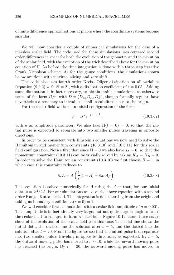
386 EXAMPLES OF NUMERICAL SPACETIMES
of finite difference approximations at places where the coordinate systems becomesingular.
We will now consider a couple of numerical simulations for the case of amassless scalar field. The code used for these simulations uses centered secondorder differences in space for both the evolution of the geometry and the evolutionof the scalar field, with the exception of the trick described above for the evolutionequation of Π. As before, the time integration is done with a three-step iterativeCrank–Nicholson scheme. As for the gauge conditions, the simulations shownbelow are done with maximal slicing and zero shift.
The code also uses fourth order Kreiss–Oliger dissipation on all variables(equation (9.9.2) with N = 2), with a dissipation coefficient of ε = 0.05. Addingsome dissipation is in fact necessary, to obtain stable simulations, as otherwiseterms of the form D/r, with D = (Dα, DA, DB), though formally regular, havenevertheless a tendency to introduce small instabilities close to the origin.
For the scalar field we take an initial configuration of the form
φ = ar2e−(r−5)2
, (10.3.67)
with a an amplitude parameter. We also take Π(t = 0) = 0, so that the ini-tial pulse is expected to separate into two smaller pulses traveling in oppositedirections.
In order to be consistent with Einstein’s equations we now need to solve theHamiltonian and momentum constraints (10.3.10) and (10.3.11) for this scalarfield configuration. Notice first that since Π = 0 we also have jA = 0, so that themomentum constraint (10.3.11) can be trivially solved by taking KA = KB = 0.In order to solve the Hamiltonian constraint (10.3.10) we first choose B = 1, inwhich case this constraint reduces to
∂rA = A
(1r(1 − A) + 8πrAρ
). (10.3.68)
This equation is solved numerically for A using the fact that, for our initialdata, ρ = Ψ2/2A. For our simulations we solve the above equation with a secondorder Runge–Kutta method. The integration is done starting from the origin andtaking as boundary condition A(r = 0) = 1.
We will consider first a simulation with a scalar field amplitude of a = 0.001.This amplitude is in fact already very large, but not quite large enough to causethe scalar field to collapse to form a black hole. Figure 10.12 shows three snap-shots of the evolution of the scalar field φ in this case: The solid line shows theinitial data, the dashed line the solution after t = 5, and the dotted line thesolution after t = 20. From the figure we see that the initial pulse first separatesinto two smaller pulses traveling in opposite directions, as expected. By t = 5,the outward moving pulse has moved to r ∼ 10, while the inward moving pulsehas reached the origin. By t = 20, the outward moving pulse has moved to

10.3 SPHERICAL SYMMETRY 387
0.02
0.00
0.02
0.04
0.06
0.08
0.10
0.12
0.14
0 5 10 15 20 25 30
Scalar field
t=0 t=20
t=5
r
Fig. 10.12: Evolution of the scalar field φ for an initial configuration with amplitudea = 0.001.
0.5
0.6
0.7
0.8
0.9
1
0 5 10 15 20 25t
Central value of
Fig. 10.13: Central value of the lapse as a function of time for an initial scalar fieldconfiguration with amplitude a = 0.001.
r ∼ 25, while the pulse that was originally moving inward has imploded throughthe origin, changing sign in the process, and is now also moving outward havingreached r ∼ 14. The evolution then proceeds with both pulses moving out andleaving flat space behind.
As we can see, the evolution of φ behaves much as we would expect for anevolution in flat space, so we might be tempted to think that spacetime is almostflat during the whole evolution. This is in fact not so, and there is a period whenspacetime has a large curvature as the inward moving pulse reaches the origin.In order to see this, Figure 10.13 shows the value of the lapse at the origin asa function of time. Notice that, just after the inward moving pulse reaches theorigin (t ∼ 5), the central value of the lapse drops to ∼ 0.6, indicating thatsignificant curvature has developed. However, since the scalar field density is notlarge enough to collapse to a black hole the central value of the lapse eventually
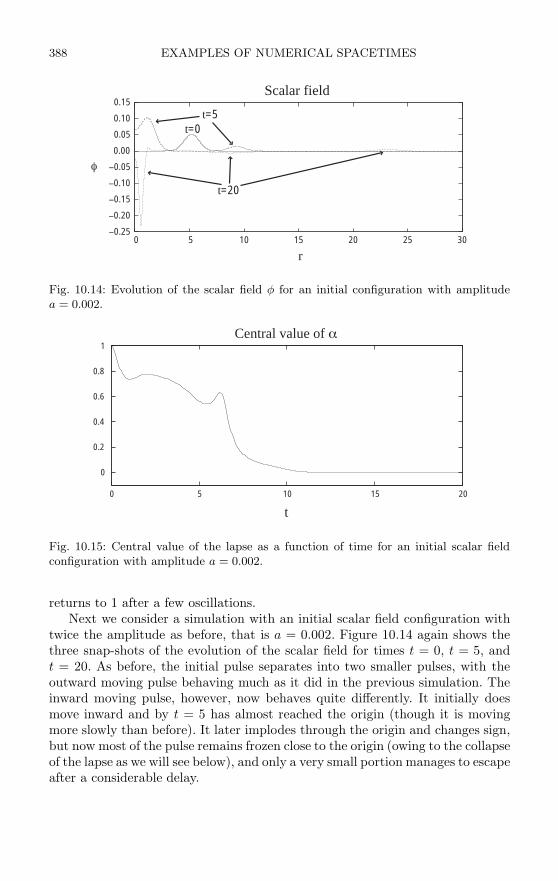
388 EXAMPLES OF NUMERICAL SPACETIMES
0.25
0.20
0.15
0.10
0.05
0.00
0.05
0.10
0.15
0 5 10 15 20 25 30
Scalar field
t=0t=5
t=20
r
Fig. 10.14: Evolution of the scalar field φ for an initial configuration with amplitudea = 0.002.
0
0.2
0.4
0.6
0.8
1
0 5 10 15 20
Central value of
t
Fig. 10.15: Central value of the lapse as a function of time for an initial scalar fieldconfiguration with amplitude a = 0.002.
returns to 1 after a few oscillations.Next we consider a simulation with an initial scalar field configuration with
twice the amplitude as before, that is a = 0.002. Figure 10.14 again shows thethree snap-shots of the evolution of the scalar field for times t = 0, t = 5, andt = 20. As before, the initial pulse separates into two smaller pulses, with theoutward moving pulse behaving much as it did in the previous simulation. Theinward moving pulse, however, now behaves quite differently. It initially doesmove inward and by t = 5 has almost reached the origin (though it is movingmore slowly than before). It later implodes through the origin and changes sign,but now most of the pulse remains frozen close to the origin (owing to the collapseof the lapse as we will see below), and only a very small portion manages to escapeafter a considerable delay.
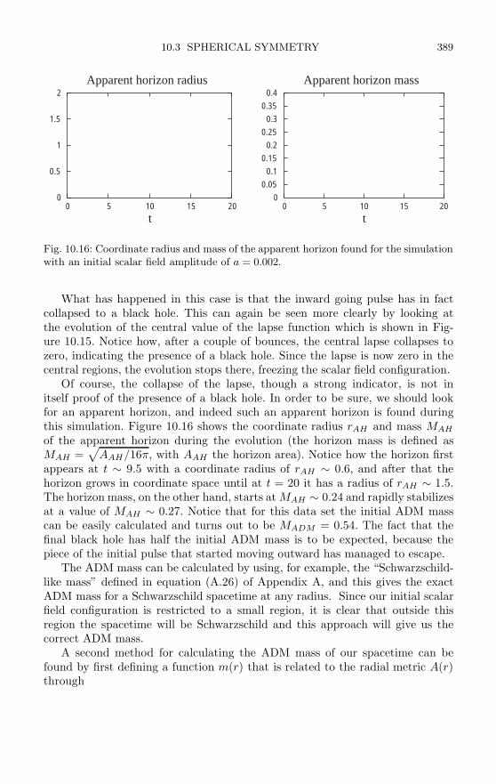
10.3 SPHERICAL SYMMETRY 389
0
0.5
1
1.5
2
0 5 10 15 20t
Apparent horizon radius
0 0.05
0.1 0.15
0.2 0.25
0.3 0.35
0.4
0 5 10 15 20t
Apparent horizon mass
Fig. 10.16: Coordinate radius and mass of the apparent horizon found for the simulationwith an initial scalar field amplitude of a = 0.002.
What has happened in this case is that the inward going pulse has in factcollapsed to a black hole. This can again be seen more clearly by looking atthe evolution of the central value of the lapse function which is shown in Fig-ure 10.15. Notice how, after a couple of bounces, the central lapse collapses tozero, indicating the presence of a black hole. Since the lapse is now zero in thecentral regions, the evolution stops there, freezing the scalar field configuration.
Of course, the collapse of the lapse, though a strong indicator, is not initself proof of the presence of a black hole. In order to be sure, we should lookfor an apparent horizon, and indeed such an apparent horizon is found duringthis simulation. Figure 10.16 shows the coordinate radius rAH and mass MAH
of the apparent horizon during the evolution (the horizon mass is defined asMAH =
√AAH/16π, with AAH the horizon area). Notice how the horizon first
appears at t ∼ 9.5 with a coordinate radius of rAH ∼ 0.6, and after that thehorizon grows in coordinate space until at t = 20 it has a radius of rAH ∼ 1.5.The horizon mass, on the other hand, starts at MAH ∼ 0.24 and rapidly stabilizesat a value of MAH ∼ 0.27. Notice that for this data set the initial ADM masscan be easily calculated and turns out to be MADM = 0.54. The fact that thefinal black hole has half the initial ADM mass is to be expected, because thepiece of the initial pulse that started moving outward has managed to escape.
The ADM mass can be calculated by using, for example, the “Schwarzschild-like mass” defined in equation (A.26) of Appendix A, and this gives the exactADM mass for a Schwarzschild spacetime at any radius. Since our initial scalarfield configuration is restricted to a small region, it is clear that outside thisregion the spacetime will be Schwarzschild and this approach will give us thecorrect ADM mass.
A second method for calculating the ADM mass of our spacetime can befound by first defining a function m(r) that is related to the radial metric A(r)through

390 EXAMPLES OF NUMERICAL SPACETIMES
0
0.1
0.2
0.3
0.4
0.5
0.6
0 5 10 15 20
t
Fig. 10.17: Mass function m(r) at t = 0 for the scalar field configuration with amplitudea = 0.002.
A(r) =1
1 − 2m(r)/r, (10.3.69)
and then rewriting the Hamiltonian constraint at t = 0, equation (10.3.68), interms of m(r). Doing this we find that the Hamiltonian constraint simplifies to:
∂rm = 4πρr2 . (10.3.70)
Notice that, since at t = 0 we are using the areal radius (B = 1), in the vacuumregion we must recover the Schwarzschild metric, which implies that m(r) mustin fact be constant and equal to the total ADM mass. We can then find the ADMmass by simply integrating the above equation up to a point where the scalarfield is negligible:
m(r) =∫ r
0
4πρr2dr , MADM = limr→∞ m(r) . (10.3.71)
It is quite remarkable that the above integral is precisely the expression for theNewtonian mass contained inside a sphere of radius r. This is a general resultin spherical symmetry as long as B = 1 and KA = KB = 0. In that case wealso finds that m(r) is precisely the Schwarzschild-like mass (A.26), so that bothmass measures coincide for all r. Figure 10.17 shows a plot of the function m(r)at t = 0. From the figure we can clearly see that m(r) increases monotonicallyin the region where the scalar field is non-zero, and settles down to a constantvalue of ∼ 0.54.
Simulations similar to those presented here, but focusing on the thresholdof black hole formation (i.e. the smallest value of the amplitude a for which ablack hole is formed), led Choptuik to the discovery of critical phenomena ingravitational collapse [98]. We will not discuss these important results here, butthe interested reader can look at e.g. [153] and references therein.
10.4 AXIAL SYMMETRY 391
10.4 Axial symmetry
As our last example of numerical spacetimes we will consider the case of axialsymmetry. Axisymmetric spacetimes have been studied in numerical relativitysince very early on. The pioneering work of Hahn and Lindquist in 1964 [158], aswell as the first successful calculations of head-on black hole collisions of Smarrand Eppley in the 1970s [123, 270, 271], were done assuming axial symmetry,and as early as 1983 there was already a beautiful review article on axisymmet-ric numerical relativity by Bardeen and Piran [48]. However, regularity issuesat both the origin and the axis of symmetry, no doubt worsened by the factthat researchers at the time were still not aware of the well-posedness problemsof the standard ADM formulation, made axisymmetric simulations particularlydifficult to keep well behaved. As a consequence of this, axisymmetric codes werepractically abandoned as soon as computers became powerful enough to be ableto handle full three-dimensional simulations in the early 1990s. Nevertheless,because of the introduction of well-posed strongly hyperbolic formulations anda better understanding of the regularity problem, it is now possible to go backto considering axisymmetric codes. Such codes have the advantage that, beingonly two-dimensional, they demand considerably less computer resource thanfull three-dimensional codes, and also they allow one to isolate the simulationsfrom possible purely three-dimensional effects (such as e.g. non-axisymmetricinstabilities).
10.4.1 Evolution equations and regularization
There are at least two different approaches to deriving evolution equations inaxisymmetry and study their regularity conditions. The simplest approach, andthe one we will consider here, is to take the standard 3+1 decomposition andrestrict it to the case of axial symmetry. However, for completeness it is importantto mention a different approach that is more geometric in nature and is basedon a decomposition of spacetime that first projects out the axial symmetry, andonly later does an ADM-like split of the resulting three-dimensional spacetime.This approach, known as the (2+1)+1 decomposition, was originally suggestedby Geroch [144] and used by Nakamura and collaborators [213], and is frequentlyused to this day (see e.g. [99]). However, as here we are just interested in somesimple aspects of axisymmetric simulations we will not discuss it further.
The first step in considering axisymmetric spacetimes is to decide on thechoice of the spatial coordinates to be used. Two different possibilities seem nat-ural, namely spherical coordinates (r, θ, ϕ) and cylindrical coordinates (ρ, z, ϕ),which are related to Cartesian coordinates (x, y, z) through
r =√
x2 + y2 + z2 , (10.4.1)
ρ =√
x2 + y2 (10.4.2)θ = arctan (z/ρ) , (10.4.3)ϕ = arctan (x/y) . (10.4.4)
392 EXAMPLES OF NUMERICAL SPACETIMES
Spherical coordinates have the advantage of being well adapted to the asymptoticboundary conditions, as well as to the propagation of gravitational waves, butthey make the regularity conditions more complicated since we have to worryabout regularity both at the origin r = 0, and at the axis of symmetry θ = 0.Because of this, here we will consider only cylindrical coordinates, for which theonly regularity problems are associated with the axis of symmetry ρ = 0.
The next step is to consider the form of the spatial metric. In the case ofspherical symmetry it was in fact possible to choose the spatial metric as diago-nal, with the two angular metric components proportional to each other so thatonly two metric components were truly independent. One might then think thatsuch a simplification of the metric is also possible in axisymmetry. Unfortunately,a little thought can convince us that this is not so in the general case, and that allsix spatial metric components must be considered independently. For example,asymptotically the metric component γzϕ corresponds to the h× polarization ofgravitational waves, so it will in general not vanish. Also, there is no reason toassume that the coordinate lines associated with z and ρ should be orthogonal,so that γρz will in general not vanish. Finally, if there is angular momentum inthe spacetime there will be dragging of inertial frames so that even if initiallywe have γρϕ = 0, this will not necessarily remain so during evolution as the ρcoordinate lines can be dragged differentially around the axis of symmetry. Insummary, all three off-diagonal components of the metric will in general be non-zero. Nevertheless, it is possible to impose the condition that γρϕ = 0 during theentire evolution by choosing appropriately the shift vector component βϕ (seee.g. [48]), and this is often done in practice.
Here, however, we will follow a different route and simplify the metric byconsidering only a restricted class of axisymmetric spacetimes, namely thosethat have zero angular momentum and no odd-parity gravitational waves (i.e.h× = 0), so that we can always take γzϕ = γρϕ = 0. In such a case the spatialmetric can be simplified to
dl2 = γρρdρ2 + γzzdz2 + 2γρzdρdz + γϕϕdϕ2
≡ Adρ2 + B dz2 + 2ρC dρdz + ρ2T dϕ2 , (10.4.5)
with the quantities (A, B, C, T ) functions of (ρ, z) only, and where we have ex-plicitly extracted some factors of ρ in order to make the regularization proceduresomewhat simpler. We can also assume that βϕ = 0, so that there are only twonon-zero shift components. Notice that with the above restrictions we can stillstudy a wide variety of interesting physical systems, such as the collapse of non-rotating stars, and even non-trivial strong gravitational wave spacetimes witheven-parity such as the Brill waves that we will discuss in the following Section.
Let us now consider the regularity of the metric functions at the axis ofsymmetry. Just as in spherical symmetry, there are two different types of reg-ularity conditions. In the first place, axial symmetry implies that the metricshould remain unchanged under the transformation ρ → −ρ, which implies that(A, B, C, T ) must all be even (and smooth) functions of ρ. As before, this can be
10.4 AXIAL SYMMETRY 393
easily implemented numerically by staggering the origin, introducing a fictitiouspoint ρ = −∆ρ/2, and setting the values of the metric variables (A, B, C, T ) atthis point by just copying them from the point ρ = +∆ρ/2.
The second type of regularity conditions are again associated with the factthat space must be locally flat at ρ = 0. In order to see where these conditionscome from, let us start from the metric components in Cartesian coordinates. Inthis case axisymmetry implies that the metric must be invariant under reflectionsabout the x and y axes and under exchange of x for y, while local flatness impliesthat it must also be smooth on the axis. These two requirements together implythat for fixed z we must have
γxx ∼ kρ + O(x2 + y2) ∼ kρ + O(ρ2) , (10.4.6)γyy ∼ kρ + O(x2 + y2) ∼ kρ + O(ρ2) , (10.4.7)γzz ∼ kz + O(x2 + y2) ∼ kz + O(ρ2) , (10.4.8)γxy ∼ O(xy) ∼ O(ρ2) , (10.4.9)γxz ∼ O(x) ∼ O(ρ) , (10.4.10)γyz ∼ O(y) ∼ O(ρ) , (10.4.11)
where kρ and kz are constants. Let us now consider a transformation to cylin-drical coordinates (ρ, z, ϕ): x = ρ cosϕ, y = ρ sinϕ, z = z. Under such a trans-formation we find
γρρ = γxx cos2 ϕ + γyy sin2 ϕ + 2γxy sinϕ cos ϕ , (10.4.12)γzz = γzz , (10.4.13)γϕϕ = ρ2
(γxx sin2 ϕ + γyy cos2 ϕ − 2γxy sinϕ cos ϕ
), (10.4.14)
γρz = γxz cosϕ + γyz sin ϕ , (10.4.15)γρϕ = ρ (γyy − γxx) sin ϕ cosϕ + ρ γxy
(cos2 ϕ − sin2 ϕ
), (10.4.16)
γzϕ = ρ (−γxz sin ϕ + γyz cosϕ) . (10.4.17)
From the behavior of the different Cartesian metric components near the axiswe then see that
γρρ ∼ kρ + O(ρ2) , (10.4.18)γzz ∼ kz + O(ρ2) , (10.4.19)γϕϕ ∼ ρ2
(kρ + O(ρ2)
), (10.4.20)
γρz ∼ O(ρ) , (10.4.21)γρϕ ∼ O(ρ3) , (10.4.22)γzϕ ∼ O(ρ2) . (10.4.23)
Going back to the definition of the functions (A, B, C, T ), we see that, closeto the axis, A and T are such that A − T ∼ O(ρ2), so that they can be writtenin general as
394 EXAMPLES OF NUMERICAL SPACETIMES
A := H + ρ2J , T := H − ρ2J , (10.4.24)
where H and J are regular functions that are even in ρ. The expressions abovecan be easily inverted to find
H :=A + T
2, J :=
A − T
2ρ2. (10.4.25)
Since the above relation between A and T must hold for all time, the componentsof the extrinsic curvature must have a similar behavior, so that we can write(again assuming no angular momentum and no odd-parity gravitational waves)
Kij =
⎛⎝ KA ρ KC 0ρ KC KB 0
0 0 ρ2KT
⎞⎠ , (10.4.26)
with KA = KH + ρ2KJ , KT = KH − ρ2KJ , and where (KH , KJ , KB, KC) areeven functions of ρ. The regularity conditions above have been derived ratherinformally; a more formal proof based on solving the Killing equation for axialsymmetry can be found in e.g. [244].
A regular system of equations in axial symmetry can now be found by simplyevolving directly the variables (H, J, KH , KJ), instead of (A, T, KA, KT ). Theevolution equations for KH and KJ can be obtained from those of KA and KT
(i.e. directly from the ADM equations or any hyperbolic reformulation of them).The resulting equations are very long and we will not write them here, but theyare trivial to obtain.
There is still, however, one important point that should be mentioned. Evenif the evolution equations for KH and KJ are regular, this regularity is notnecessarily apparent and care must be taken with some terms that are irregularon their own but become regular when added together. Such terms typically havethe form
1ρ2
(∂ρD − D
ρ
), (10.4.27)
with D the derivative of either the lapse, or some combination of the metriccoefficients (A, B, C, T ), with respect to either ρ or z. Since such derivativesbehave as O(ρ) near the axis, the term above seems to be ill-behaved. However,it is easy to see that
1ρ2
(∂ρD − D
ρ
)=
1ρ
∂ρ
(D
ρ
). (10.4.28)
The term on the right hand side is now clearly regular since D/ρ ∼ 1 + O(ρ2).The specific form of such terms depends on the details of the formulation beingused (i.e. ADM, BSSNOK, NOR, etc.), and the equations must be carefullyinspected before writing a numerical code (see e.g. [245]).
10.4 AXIAL SYMMETRY 395
10.4.2 Brill waves
As an example of the evolution of an axially symmetric spacetime we will con-sider a non-trivial system consisting of strong non-linear gravitational waves invacuum, commonly known as Brill waves [78, 124, 125]. The construction of sucha spacetime starts by considering an axisymmetric initial slice with a metric ofthe form
ds2 = Ψ4[e2q(dρ2 + dz2
)+ ρ2dϕ2
], (10.4.29)
with (ρ, z, ϕ) cylindrical coordinates, and where both q and Ψ are functions of(t, ρ, z) only. The function q is quasi-arbitrary, and must only satisfy the followingboundary conditions
q |ρ=0 = 0 , (10.4.30)∂n
ρ q |ρ=0 = 0 for odd n , (10.4.31)
q |r→∞ = O(r−2)
, (10.4.32)
where r =√
ρ2 + z2. In order to find the conformal factor Ψ, we first imposethe condition of time symmetry, which implies that the momentum constraintsare identically satisfied. The Hamiltonian constraint, on the other hand, takesthe form
D2flatΨ +
14(∂2ρq + ∂2zq
)Ψ = 0 , (10.4.33)
with D2flat the flat space Laplacian. Since this is an elliptic equation we must
also say something about the boundary conditions. At infinity we must clearlyhave Ψ = 1; however since our computational domain is finite we must ask forboundary condition at a finite distance. Notice that we expect that far away thesolution should approach a Schwarzschild spacetime, which implies that Ψ mustbehave asymptotically as Ψ ∼ 1 + M/2r. This provides us with our boundarycondition for large r.
Once a function q has been chosen, all we need to do is solve the above ellipticequation numerically for Ψ. Different forms of the function q have been used bydifferent authors [124, 125, 163, 267]. Here we will consider the one introducedby Holz and collaborators in [163], which has the form
q = aρ2e−(ρ2+z2) , (10.4.34)
with a a constant that determines the initial amplitude of the wave (for smalla the waves should disperse to infinity, while for large a they should collapse toform a black hole).
Before considering any evolutions, let us first discuss the solution of the ini-tial data, which involves solving the elliptic equation (10.4.33) numerically. InChapter 9 we did not discuss the solution of elliptic equations, but here we canpresent a quick and dirty method that is very easy to code (it is also extremelyinefficient, so the reader should not use it for any serious applications). The
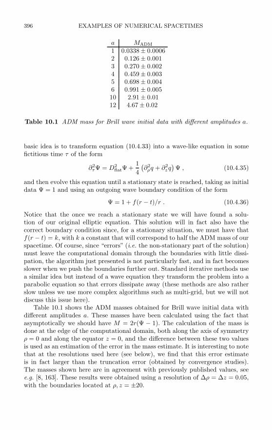
396 EXAMPLES OF NUMERICAL SPACETIMES
a MADM
1 0.0338± 0.00062 0.126 ± 0.0013 0.270 ± 0.0024 0.459 ± 0.0035 0.698 ± 0.0046 0.991 ± 0.00510 2.91 ± 0.0112 4.67 ± 0.02
Table 10.1 ADM mass for Brill wave initial data with different amplitudes a.
basic idea is to transform equation (10.4.33) into a wave-like equation in somefictitious time τ of the form
∂2τΨ = D2flatΨ +
14(∂2ρq + ∂2zq
)Ψ , (10.4.35)
and then evolve this equation until a stationary state is reached, taking as initialdata Ψ = 1 and using an outgoing wave boundary condition of the form
Ψ = 1 + f(r − t)/r . (10.4.36)
Notice that the once we reach a stationary state we will have found a solu-tion of our original elliptic equation. This solution will in fact also have thecorrect boundary condition since, for a stationary situation, we must have thatf(r − t) = k, with k a constant that will correspond to half the ADM mass of ourspacetime. Of course, since “errors” (i.e. the non-stationary part of the solution)must leave the computational domain through the boundaries with little dissi-pation, the algorithm just presented is not particularly fast, and in fact becomesslower when we push the boundaries further out. Standard iterative methods usea similar idea but instead of a wave equation they transform the problem into aparabolic equation so that errors dissipate away (these methods are also ratherslow unless we use more complex algorithms such as multi-grid, but we will notdiscuss this issue here).
Table 10.1 shows the ADM masses obtained for Brill wave initial data withdifferent amplitudes a. These masses have been calculated using the fact thatasymptotically we should have M = 2r(Ψ − 1). The calculation of the mass isdone at the edge of the computational domain, both along the axis of symmetryρ = 0 and along the equator z = 0, and the difference between these two valuesis used as an estimation of the error in the mass estimate. It is interesting to notethat at the resolutions used here (see below), we find that this error estimateis in fact larger than the truncation error (obtained by convergence studies).The masses shown here are in agreement with previously published values, seee.g. [8, 163]. These results were obtained using a resolution of ∆ρ = ∆z = 0.05,with the boundaries located at ρ, z = ±20.
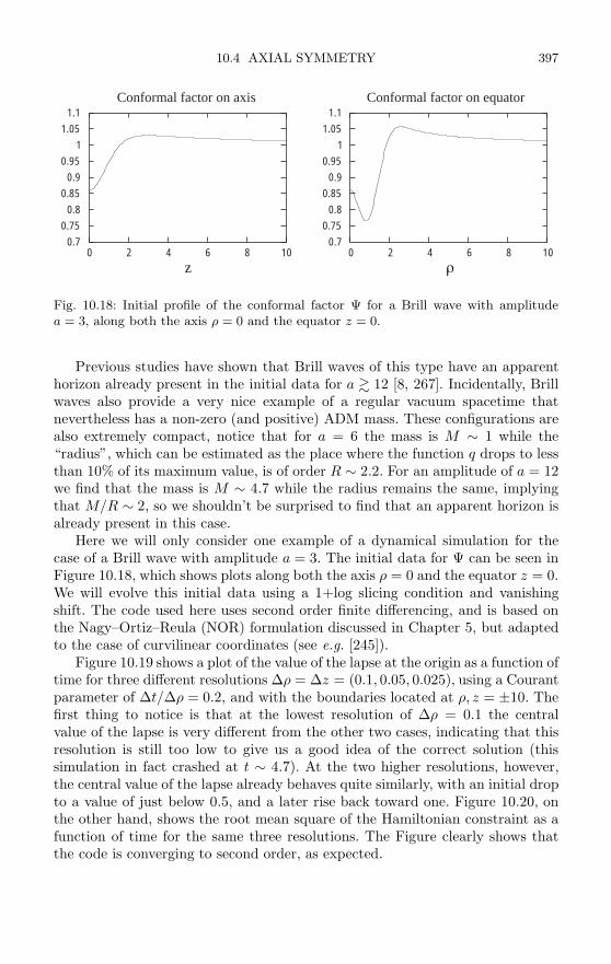
10.4 AXIAL SYMMETRY 397
0.7 0.75
0.8 0.85
0.9 0.95
1 1.05
1.1
0 2 4 6 8 10z
Conformal factor on axis
0.7 0.75
0.8 0.85
0.9 0.95
1 1.05
1.1
0 2 4 6 8 10
Conformal factor on equator
Fig. 10.18: Initial profile of the conformal factor Ψ for a Brill wave with amplitudea = 3, along both the axis ρ = 0 and the equator z = 0.
Previous studies have shown that Brill waves of this type have an apparenthorizon already present in the initial data for a 12 [8, 267]. Incidentally, Brillwaves also provide a very nice example of a regular vacuum spacetime thatnevertheless has a non-zero (and positive) ADM mass. These configurations arealso extremely compact, notice that for a = 6 the mass is M ∼ 1 while the“radius”, which can be estimated as the place where the function q drops to lessthan 10% of its maximum value, is of order R ∼ 2.2. For an amplitude of a = 12we find that the mass is M ∼ 4.7 while the radius remains the same, implyingthat M/R ∼ 2, so we shouldn’t be surprised to find that an apparent horizon isalready present in this case.
Here we will only consider one example of a dynamical simulation for thecase of a Brill wave with amplitude a = 3. The initial data for Ψ can be seen inFigure 10.18, which shows plots along both the axis ρ = 0 and the equator z = 0.We will evolve this initial data using a 1+log slicing condition and vanishingshift. The code used here uses second order finite differencing, and is based onthe Nagy–Ortiz–Reula (NOR) formulation discussed in Chapter 5, but adaptedto the case of curvilinear coordinates (see e.g. [245]).
Figure 10.19 shows a plot of the value of the lapse at the origin as a function oftime for three different resolutions ∆ρ = ∆z = (0.1, 0.05, 0.025), using a Courantparameter of ∆t/∆ρ = 0.2, and with the boundaries located at ρ, z = ±10. Thefirst thing to notice is that at the lowest resolution of ∆ρ = 0.1 the centralvalue of the lapse is very different from the other two cases, indicating that thisresolution is still too low to give us a good idea of the correct solution (thissimulation in fact crashed at t ∼ 4.7). At the two higher resolutions, however,the central value of the lapse already behaves quite similarly, with an initial dropto a value of just below 0.5, and a later rise back toward one. Figure 10.20, onthe other hand, shows the root mean square of the Hamiltonian constraint as afunction of time for the same three resolutions. The Figure clearly shows thatthe code is converging to second order, as expected.
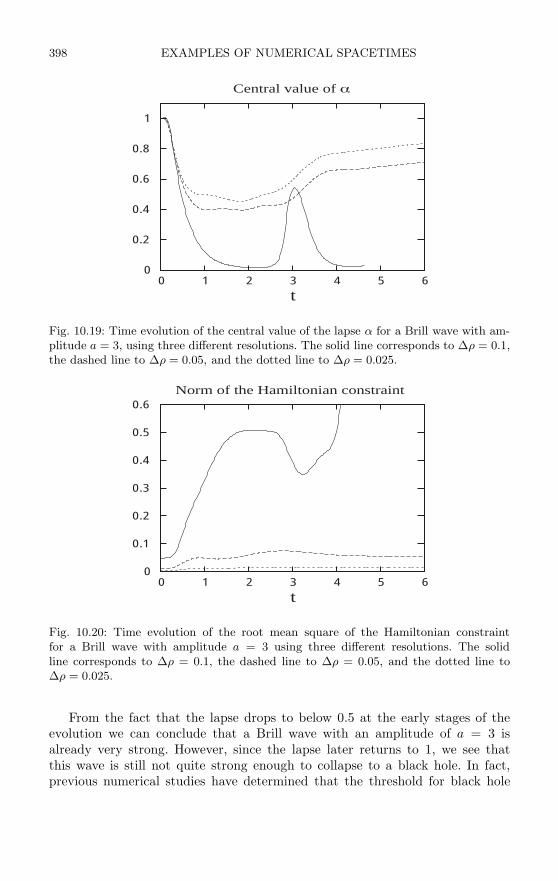
398 EXAMPLES OF NUMERICAL SPACETIMES
0
0.2
0.4
0.6
0.8
1
0 1 2 3 4 5 6t
Central value of
Fig. 10.19: Time evolution of the central value of the lapse α for a Brill wave with am-plitude a = 3, using three different resolutions. The solid line corresponds to ∆ρ = 0.1,the dashed line to ∆ρ = 0.05, and the dotted line to ∆ρ = 0.025.
0
0.1
0.2
0.3
0.4
0.5
0.6
0 1 2 3 4 5 6t
Norm of the Hamiltonian constraint
Fig. 10.20: Time evolution of the root mean square of the Hamiltonian constraintfor a Brill wave with amplitude a = 3 using three different resolutions. The solidline corresponds to ∆ρ = 0.1, the dashed line to ∆ρ = 0.05, and the dotted line to∆ρ = 0.025.
From the fact that the lapse drops to below 0.5 at the early stages of theevolution we can conclude that a Brill wave with an amplitude of a = 3 isalready very strong. However, since the lapse later returns to 1, we see thatthis wave is still not quite strong enough to collapse to a black hole. In fact,previous numerical studies have determined that the threshold for black hole

10.4 AXIAL SYMMETRY 399
x
y
Fig. 10.21: The Cartoon approach: The points on the y = 0 plane are evolved usingstandard three-dimensional finite differencing. Those on the adjacent planes are thenobtained by rotating around the z axis and interpolating.
formation corresponds to an amplitude of a ∼ 5 [5]. Simulations with such largeamplitudes, however, are extremely hard to do since the dynamics are so strongthat numerical instabilities become very difficult to control, and because of thiswe will not consider them here.106
10.4.3 The “Cartoon” approach
Before finishing this Chapter it is important to mention a different approach tothe evolution of axisymmetric spacetimes. This approach in commonly known asthe “Cartoon” technique [9], and consists of evolving an axisymmetric spacetimeusing a three-dimensional code with a computational domain that is only a fewgrid points thick (typically 3 or 5) in the y direction, i.e. we consider only a thinslab consisting of the y = 0 plane plus one or two more planes on either side.107
The field variables in the central y = 0 plane can then be updated using standardCartesian finite differencing, while those in the extra y = 0 planes can be com-puted from the data in the central plane by making tensor rotations around the zaxis, and then interpolating to the desired grid point (see Figure 10.21). In otherwords, the boundary conditions on the y direction are obtained by enforcingaxial symmetry on all tensor quantities.
In order to apply the Cartoon approach it is necessary to consider the effecton tensor quantities of a rotation around the z axis. Assume that we are usingcylindrical coordinates (ρ, z, ϕ). A rotation around the z axis can then be seenas the following change of coordinates
ρ′ = ρ , ϕ′ = ϕ + ϕ0 , z′ = z , (10.4.37)
106In fact, the code described above already requires a very large Kreiss–Oliger dissipationparameter in order to handle the a = 3 case.107The original idea, as well as the name, were first suggested by S. Brandt. The name makes
reference to the fact the we use a Cartesian code to do a two-dimensional simulation, that isCartesian-2D or simply “Cartoon”.
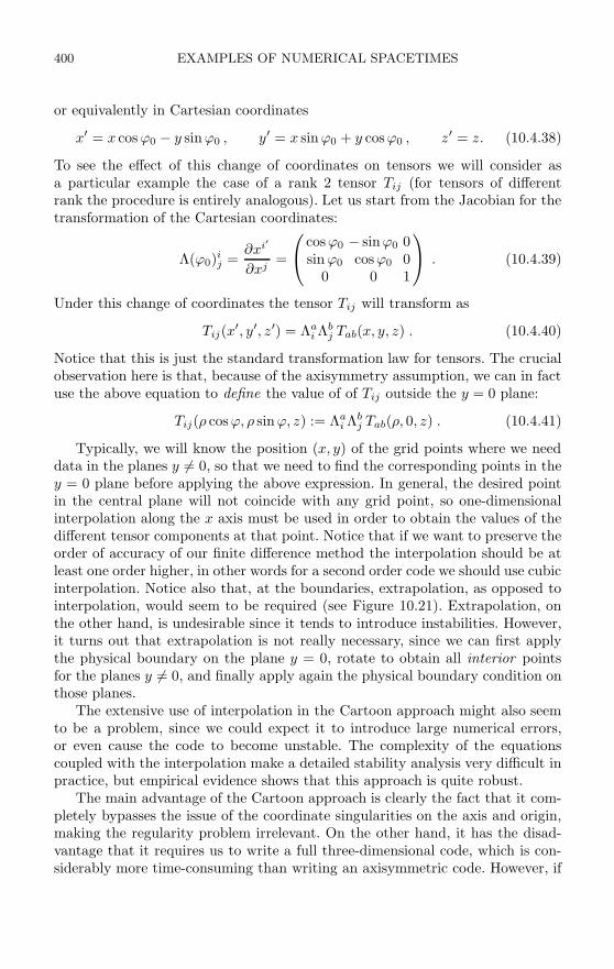
400 EXAMPLES OF NUMERICAL SPACETIMES
or equivalently in Cartesian coordinates
x′ = x cos ϕ0 − y sin ϕ0 , y′ = x sin ϕ0 + y cosϕ0 , z′ = z. (10.4.38)
To see the effect of this change of coordinates on tensors we will consider asa particular example the case of a rank 2 tensor Tij (for tensors of differentrank the procedure is entirely analogous). Let us start from the Jacobian for thetransformation of the Cartesian coordinates:
Λ(ϕ0)ij =
∂xi′
∂xj=
⎛⎝ cosϕ0 − sinϕ0 0sin ϕ0 cosϕ0 0
0 0 1
⎞⎠ . (10.4.39)
Under this change of coordinates the tensor Tij will transform as
Tij(x′, y′, z′) = Λai Λb
j Tab(x, y, z) . (10.4.40)
Notice that this is just the standard transformation law for tensors. The crucialobservation here is that, because of the axisymmetry assumption, we can in factuse the above equation to define the value of of Tij outside the y = 0 plane:
Tij(ρ cosϕ, ρ sinϕ, z) := Λai Λb
j Tab(ρ, 0, z) . (10.4.41)
Typically, we will know the position (x, y) of the grid points where we needdata in the planes y = 0, so that we need to find the corresponding points in they = 0 plane before applying the above expression. In general, the desired pointin the central plane will not coincide with any grid point, so one-dimensionalinterpolation along the x axis must be used in order to obtain the values of thedifferent tensor components at that point. Notice that if we want to preserve theorder of accuracy of our finite difference method the interpolation should be atleast one order higher, in other words for a second order code we should use cubicinterpolation. Notice also that, at the boundaries, extrapolation, as opposed tointerpolation, would seem to be required (see Figure 10.21). Extrapolation, onthe other hand, is undesirable since it tends to introduce instabilities. However,it turns out that extrapolation is not really necessary, since we can first applythe physical boundary on the plane y = 0, rotate to obtain all interior pointsfor the planes y = 0, and finally apply again the physical boundary condition onthose planes.
The extensive use of interpolation in the Cartoon approach might also seemto be a problem, since we could expect it to introduce large numerical errors,or even cause the code to become unstable. The complexity of the equationscoupled with the interpolation make a detailed stability analysis very difficult inpractice, but empirical evidence shows that this approach is quite robust.
The main advantage of the Cartoon approach is clearly the fact that it com-pletely bypasses the issue of the coordinate singularities on the axis and origin,making the regularity problem irrelevant. On the other hand, it has the disad-vantage that it requires us to write a full three-dimensional code, which is con-siderably more time-consuming than writing an axisymmetric code. However, if
10.4 AXIAL SYMMETRY 401
we already have a three-dimensional code available, adapting it to do axisym-metric simulations using the Cartoon method should be quite straightforward.The main idea can, of course, also be used for spherical symmetry by consideringa thin pencil of grid points centered around the x axis that is only a few gridpoints thick along the y and z directions, though spherical symmetry is usuallysufficiently simple on its own so that using the Cartoon method is probably notnecessary.
APPENDIX A
TOTAL MASS AND MOMENTUM IN GENERAL RELATIVITY
The concept of energy is of fundamental importance in most physical theories.Indeed, even in relativity the stress-energy tensor of matter T µν plays a keyrole both in the conservation laws, from which the dynamics can often by fullydetermined, and as a source of the gravitational field. In general relativity, thestress-energy tensor satisfies a conservation law of the form ∇νT µν = 0, but incontrast to special relativity this local conservation law does not lead to globalconservation of energy integrated over a finite volume. The reason is clear, asT µν represents only the energy of matter and does not take into account thecontribution from the gravitational field. However, it turns out that, in relativity,we can in general not define the energy density of the gravitational field itself.
On the other hand, in general relativity we can in fact define the total energyof an isolated system in a meaningful way. We will consider here two differentapproaches to defining both the total energy and the momentum of an asymp-totically flat spacetime. The presentation here will be brief and not rigorous; fora more rigorous discussion see e.g. [31, 222, 306].
The first approach is motivated by considering weak gravitational fields forwhich gµν = ηµν + hµν , with |hµν | 1. In such a case, it is clear that thetotal mass (energy) and momentum can be defined as the integral of the energydensity ρ and momentum density ji of matter, respectively
M =∫
ρ dV , Pi =∫
ji dV . (A.1)
Using now the Hamiltonian and momentum constraints of the 3+1 formalism,equations (2.4.10) and (2.4.11), plus the fact that, in the weak field limit, theextrinsic curvature Kij is itself a small quantity, we can rewrite this as (in allfollowing expressions sum over repeated indices is understood)
M =1
16π
∫R dV , Pi =
18π
∫∂j (Kij − δijK) dV , (A.2)
where R is the Ricci scalar of the spatial metric, which in the linearized theoryis given by
R = ∂j (∂ihij − ∂jh) , (A.3)
with h the trace of hij . Notice that both the mass and momentum are nowwritten as volume integrals of a divergence, so using Gauss’ theorem we canrewrite them as
402
TOTAL MASS AND MOMENTUM IN GENERAL RELATIVITY 403
M =1
16π
∮S
(∂ihij − ∂jh) dSj , Pi =18π
∮S
(Kij − δijK) dSj , (A.4)
where the integrals are calculated over surfaces outside the matter sources, andwhere γij = δij + hij is the spatial metric and dSi = sidA, with si the unitoutward-pointing normal vector to the surface and dA the area element. Theexpressions above are called the ADM mass and ADM momentum of the space-time (ADM stands for Arnowitt, Deser, and Misner [31]). Notice that the ADMmass depends only on the behavior of the spatial metric, while the ADM mo-mentum depends on the extrinsic curvature instead. We should stress the factthat for these expressions to hold we must be working with quasi-Minkowski, i.e.Cartesian type, coordinates.
In order to derive the ADM integrals above, we started from the weak fieldtheory and used Gauss’ theorem to transform the volume integrals into surfaceintegrals. In the case of strong gravitational fields, the total mass and momentumcan not be expected to be given directly by the volume integrals of the energy andmomentum densities, precisely because these integrals fail to take into accountthe effect of the gravitational field. However, we in fact define the total mass andmomentum of an isolated system through its gravitational effects on farawaytest masses, and far away the weak field limit does hold, so the surface integralsabove will still give the correct values we physically associate with the total massand momentum, but they must be evaluated at infinity to guarantee that we arein the weak field regime. We then define the ADM mass and momentum in thegeneral case as
MADM =1
16πlim
r→∞
∮S
(δij∂ihjk − ∂kh
)dSk , (A.5)
P iADM =
18π
limr→∞
∮S
(Ki
j − δijK)
dSj , (A.6)
Using the same idea we can also construct a measure of the total angularmomentum J i of the system starting from the density of angular momentumgiven by εijkxjjk, with xi Cartesian coordinates (this is just r × j in standardthree-dimensional vector notation). The ADM angular momentum then becomes
J iADM =
18π
limr→∞
∮S
εijkxj (Kkl − δklK) dSl . (A.7)
Notice that, in fact, in the limit r → ∞, the term proportional to K can bedropped out since at spatial infinity the Cartesian vector x is collinear with thearea element dS so that εijlxjdSl = 0. The integral can then be rewritten as
J iADM =
18π
limr→∞
∮S
εijkxjKkl dSl . (A.8)
In particular, for the projection along the z axis we find

404 TOTAL MASS AND MOMENTUM IN GENERAL RELATIVITY
JzADM =
18π
limr→∞
∮S
εzjkxjKkl dSl
=18π
limr→∞
∮S
ϕkKkl dSl , (A.9)
with ϕ the coordinate basis vector associated with the azimuthal angle ϕ.There is a very important property of the ADM mass and momentum defined
above. Since these quantities are defined at spatial infinity i0, and since anygravitational waves taking energy and momentum away from the system willinstead reach null infinity J +, the ADM mass and momentum will remainconstant during the evolution of the system.
The expression for the ADM mass given in (A.5) has the disadvantage that itis not covariant and must be calculated in Cartesian-type coordinates. This canin fact be easily remedied. In an arbitrary curvilinear coordinate system definethe tensor hij := γij −γ0ij, with γ0ij the metric of flat space expressed in the samecoordinates. It is easy to convince oneself that hij does indeed transform like atensor. We can now rewrite the ADM mass as
MADM =1
16πlim
r→∞
∮S
(D0
jhjk − D0
kh)
dSk , (A.10)
where D0i is the covariant derivative with respect to the flat metric γ0ij in the
corresponding curvilinear coordinates, and where indices are raised and loweredalso with γ0ij . Notice that the tensor hij is not unique because we can still makeinfinitesimal coordinate transformations that will change hij without changingD0
jhjk − D0
kh (gauge transformations in the context of linearized theory).From the last result we can also obtain a particularly useful expression for
the ADM mass:
MADM =18π
limr→∞
∮S
(k − k0
)dA , (A.11)
where dA is the area element of the surface S, k is the trace of the extrinsiccurvature of S, and k0 is the trace of the extrinsic curvature of S when em-bedded in flat space.108 It is important to mention that the surface S, whenembedded in flat space, must have the same intrinsic curvature as it did whenembedded in curved space. The derivation of this expression is not difficult andcan be obtained by considering an adapted coordinate system, with one of thecoordinates measuring proper distance along the normal direction and the othertwo coordinates transported orthogonally off S; see for example [227] (in 3+1terms, we would have a “lapse” equal to 1 and zero “shift”, but in this case theorthogonal direction is spacelike and the surface is bi-dimensional).
108This expression for the ADM mass is due to Katz, Lynden-Bell, and Israel [169] (seealso [227], but notice that our definition of extrinsic curvature has a sign opposite to thatreference).
TOTAL MASS AND MOMENTUM IN GENERAL RELATIVITY 405
In the case when the spatial metric is conformally flat, i.e. γij = ψ4δij , theexpression for the ADM mass simplifies considerably and reduces to [222]
MADM = − 12π
limr→∞
∮S
∂jψ dSj , (A.12)
where we have assumed that far away ψ becomes unity.
There is another common approach to defining global energy and momentumthat works for spacetimes that have a Killing field ξµ. I will give here a roughderivation of the corresponding expressions; a more formal derivation can befound in e.g. [108]. Notice first that for any antisymmetric tensor Aµν we have
|g|1/2∇νAµν = ∂ν
(|g|1/2Aµν
), (A.13)
|g|1/2∇µ∇νAµν = ∂µ∂ν
(|g|1/2Aµν
)= 0 . (A.14)
Integrating the second expression above and using Gauss’ theorem we find
0 =∫Ω
∇µ∇νAµνdΩ =∫Ω
|g|1/2∇µ∇νAµνd4x
=∫Ω
∂µ∂ν
(|g|1/2Aµν
)d4x =
∮∂Ω
∂ν
(|g|1/2Aµν
)nµ d3x , (A.15)
where Ω is some four-dimensional region of spacetime, ∂Ω is its boundary andnµ is the unit outward-pointing normal vector to the boundary, with the normdefined using a flat metric. Assume now that Ω is the region bounded by twospacelike hypersurfaces Σ1 and Σ2 (with Σ1 to the future of Σ2), and a timelikecylindrical world-tube σ. We then find∫
Σ1
∂ν
(|g|1/2Aµν
)nµ d3x −
∫Σ2
∂ν
(|g|1/2Aµν
)nµ d3x
+∫
σ
∂ν
(|g|1/2Aµν
)nµ d3x = 0 , (A.16)
where in both the integrals over Σ1 and Σ2 the normal vector nµ is taken to befuture pointing.
Take now Aµν = ∇µξν , which will be antisymmetric if ξµ is a Killing vector.For the integrals over the timelike cylinder we then have∫
σ
∂ν
(|g|1/2∇µξν
)nµ d3x =
∫σ
|g|1/2 (∇ν∇µξν) nµ d3x
=∫
σ
|g|1/2Rµνξν nµ d3x
= 8π
∫σ
|g|1/2(
T µν − 12gµνT
)ξν nµ d3x , (A.17)
where Rµν is the Ricci tensor and Tµν the stress-energy tensor of matter. Inthe second line above we used the Ricci identity to relate the commutator of

406 TOTAL MASS AND MOMENTUM IN GENERAL RELATIVITY
covariant derivatives to the Riemann tensor (1.9.3) plus the fact that ξµ is aKilling field, and in the third line the Einstein field equations. If we now assumethat we have an isolated source and the cylindrical world-tube is outside it thenthe above integral clearly vanishes. Equation (A.16) then implies that∫
Σ1
∂ν
(|g|1/2∇µξν
)nµ d3x =
∫Σ2
∂ν
(|g|1/2∇µξν
)nµ d3x , (A.18)
This means that the spatial integral is in fact independent of the hypersurfaceΣ chosen, or in other words, the spatial integral is a conserved quantity.
To proceed further we choose coordinates such that nµ = δµ0 . Using the fact
that ∇µξν is antisymmetric, and applying again Gauss’ theorem, the spatialintegral becomes∫
Σ
∂i
(|g|1/2∇0ξi
)d3x =
∮∂Σ
|g|1/2∇0ξi si d2x
=∮
∂Σ
|g|1/2∇µξν sν nµ d2x , (A.19)
where ∂Σ is now the two-dimensional boundary of Σ and sµ is the spatial unitoutward-pointing normal vector to ∂Σ. In the last expression we can notice that|g|1/2nµsν d2x = nµsν dA, where now nµ and sµ are unit vectors with respectto the full curved metric gµν , and dA is the proper area element of ∂Σ. We canthen write the integral as
IK
(ξ)
:= − 14π
∮∂Σ
sµnν∇µξν dA . (A.20)
This is known as the Komar integral [176] and as we have seen is a conservedquantity (the quantity Aµν = ∇µξν is also frequently called the Komar poten-tial).109 The integral can in fact be calculated over any surface ∂Σ outside thematter sources. The normalization factor −1/4π has been chosen to ensure that,for the case of a timelike Killing field that has unit magnitude at infinity, theKomar integral will coincide with the ADM mass of the spacetime. If, on theother hand, ξµ is an axial vector associated with an angular coordinate φ (i.e.ξµ = δµ
φ), then the Komar integral turns out to be −2J , with J the total angularmomentum (we can check that this is so by considering a Kerr black hole). Thefact that, for a static spacetime, the Komar integral and the ADM mass coincidecan be used to derive a general relativistic version of the virial theorem, but wewill not consider this issue here (the interested reader can see e.g. [69]).
109The Komar integral is usually written in differential form notation as
IK = − 1
4π
I∇µξνdSµν = − 1
8π
Iεµναβ∇µξν dxα ∧ dxβ .
In fact, in the last expression, the area element dxα ∧ dxβ is frequently not even written.
TOTAL MASS AND MOMENTUM IN GENERAL RELATIVITY 407
Incidentally, we can use the same derivation that allowed us to show that theintegral over the timelike cylinder σ vanishes to rewrite the Komar integral as avolume integral of the stress-energy of matter as
IK
(ξ)
:= 2∫Σ
(T µν − 1
2gµνT
)nµξν dV , (A.21)
with dV the proper volume element of the spatial hypersurface.The Komar integral can in fact also be used to define mass at null infinity
J + in the case of non-stationary asymptotically flat spacetimes. This is knownas the Bondi mass, and is defined as
MB := − 14π
limS→J
∮S
sµnν∇µξν dA , (A.22)
where now ξµ is assumed to be the generator of an asymptotic time translationsymmetry, and where the surface of integration is now taken to approach a crosssection J of J + (when ξµ is not an exact Killing field we must ask for an extranormalization condition, see e.g. [295]). While the ADM mass measures the totalenergy available in a spacetime, the Bondi mass represents the remaining energyat a retarded time. This means that, in particular, the Bondi mass can be used tocalculate the change in the total energy of an isolated system that goes througha phase in which it radiates gravitational waves.
Before finishing this Appendix it is important to mention that the ADMexpressions for mass and momentum given above, though correct, in practiceconverge very slowly as r goes to infinity, so that if we evaluate them at a finiteradius in a numerical simulation the errors might be quite large. We can of courseevaluate them at several radii and then extrapolate to the asymptotic value. Forthe mass, however, there are other approaches that work well in practice. Onesuch approach is based on the use of the so-called Hawking mass, which is a quasi-local measure of energy defined for any given closed surface S as (see e.g. [276])
MH :=
√A
16π
(1 +
116π
∮S
HinHoutdS
), (A.23)
where A is the area of the surface, and Hin and Hout are the expansions of theingoing and outgoing null geodesics which are given in terms of 3+1 quantitiesas (see equation (6.7.8))
Hin = Kmnsmsn − K − Dmsm , (A.24)Hout = Kmnsmsn − K + Dmsm , (A.25)
with s being the unit outward-pointing normal vector to S, and Di the standardthree-dimensional covariant derivative. The Hawking mass is defined by thinkingthat the presence of a mass must cause light rays to converge, and it turns

408 TOTAL MASS AND MOMENTUM IN GENERAL RELATIVITY
out that the only gauge invariant measure of this on the surface is given byHinHout.110 We would then expect the mass to be given by an expression of theform M = A + B
∮HinHoutdS, with the constants A and B fixed by looking at
special cases.For spheres in Minkowski spacetime the Hawking mass vanishes identically
since Hin = −Hout = 2/r. For spheres in Schwarzschild (in standard coordinates)we have Hin = −Hout = 2(1 − 2M/r)1/2/r and A = 4πr2, so that MH = M .That is, the Hawking mass gives us the correct mass at all radii, which makesit a more useful measure of energy than the ADM mass. The Hawking mass ingeneral is not always positive definite, and is not always monotonic either, butfor sufficiently “round” surfaces (and particularly in spherical symmetry) boththese properties can be shown to be satisfied if the dominant energy conditionholds.
Another less formal but very useful approach to obtaining a local expressionfor the mass of the spacetime is based on the fact that many astrophysicallyrelevant spacetimes will not only be asymptotically flat, but they will also beasymptotically spherically symmetric. In such a case we know that the spacetimewill approach Schwarzschild far away. For Schwarzschild we can easily prove thefollowing exact relation between the mass M and the area A of spheres
M =(
A
16π
)1/2 [1 − (dA/dr)2
16πgrrA
], (A.26)
where r is some arbitrary radial coordinate. In numerical simulations of space-times that are asymptotically spherically symmetric we can calculate the area Aof coordinate spheres at finite radii, the rate of change of the area with radiusdA/dr, and the average radial metric over the sphere grr, and then use the aboveexpression to estimate the mass. In practice we often find that as r is increasedthis “Schwarzschild-like” mass converges very rapidly to the correct ADM mass,much more rapidly than the ADM integral itself. This works even for spacetimeswith non-zero angular momentum like Kerr, as the angular momentum terms inthe metric decay faster than the mass term.
110More specifically, the product of the Newman–Penrose spin coefficients ρ and ρ′ is gaugeinvariant under a spin-boost transformation of the null tetrad, and in general it is given byρρ′ = HinHout/8.
APPENDIX B
SPACETIME CHRISTOFFEL SYMBOLS IN 3+1 LANGUAGE
In the derivation of 3+1 equations we often need to write the 4-metric of space-time and its associated Christoffel symbols in 3+1 language. The 4-metric interms of 3+1 quantities has the form
g00 = − (α2 − γij βiβj)
, (B.1)
g0i = γij βj = βi , (B.2)gij = γij , (B.3)
and the corresponding inverse metric is
g00 = −1/α2 , (B.4)g0i = βi/α2 , (B.5)gij = γij − βiβj/α2 . (B.6)
From this we can obtain the following expressions for the 4-Christoffel sym-bols in terms of 3+1 quantities
Γ000 = (∂t α + βm∂m α − βmβnKmn) /α , (B.7)Γ00i = (∂iα − βmKim) /α , (B.8)Γ0ij = −Kij/α , (B.9)
Γl00 = α∂lα − 2αβmK l
m − βl (∂tα + βm∂mα − βmβnKmn) /α
+ ∂tβl + βm Dmβl , (B.10)
Γlm0 = −βl (∂mα − βnKmn) /α − αK l
m + Dmβl , (B.11)Γl
ij = (3)Γlij + βlKij/α , (B.12)
with Di the covariant derivative associated with the spatial metric γij , and (3)Γlij
the corresponding three-dimensional Christoffel symbols. The 3-covariant deriva-tives of the shift that appear in these expressions come from partial derivativesof the metric along the time direction contained in the Γα
µν .The contracted Christoffel symbols Γα := gµνΓα
µν then become
Γ0 = − 1α3(∂tα − βm∂mα + α2K
), (B.13)
Γi = (3)Γi +βi
α3(∂tα − βm∂mα + α2K
)− 1
α2(∂tβ
i − βm∂mβi + α∂iα)
. (B.14)
409

APPENDIX C
BSSNOK WITH NATURAL CONFORMAL RESCALING
The BSSNOK formulation of the 3+1 evolution equations described in Sec-tion 2.8 is based on a conformal rescaling of the metric and extrinsic curvature.However, in its standard version this formulation uses a rescaling of the extrinsiccurvature that is in fact not the most natural rescaling for this quantity. Here Iwill present a version of the BSSNOK equations that uses the natural rescalingfor a tracefree symmetric tensor.
We start by summarizing the standard BSSNOK equations. We perfom aconformal transformation of the spatial metric and extrinsic curvature of theform
γij := e−4φ γij , (C.1)
Aij := e−4φ(
Kij − 13γijK
), (C.2)
where the conformal factor is taken to be φ = 112 ln γ, so that the conformal
metric γij has unit determinant. In the previous expression K is the trace of Kij ,which implies that the tensor Aij is traceless. We also introduces the auxiliaryvariables
Γi = γjkΓijk = −∂j γ
ij , (C.3)
where the second equality follows from the fact that γij has unit determinant.The full system of evolution equations then becomes
d
dtγij = −2αAij , (C.4)
d
dtφ = −1
6αK , (C.5)
d
dtK = −DiD
iα + α
(AijA
ij +13K2
)+ 4πα (ρ + S) , (C.6)
d
dtAij = e−4φ
−DiDjα + αRij + 4πα [γij (S − ρ) − 2Sij ]
TF+ α
(KAij − 2AikAk
j
), (C.7)
d
dtΓi = γjk∂j∂kβi +
13
γij∂j∂kβk − 2Aij∂jα
+ 2α
(Γi
jkAjk + 6Aij∂jφ − 23γij∂jK − 8πe4φji
), (C.8)
410

BSSNOK WITH NATURAL CONFORMAL RESCALING 411
where TF denotes the tracefree part of the expression inside the brackets, andwhere we have used the Hamiltonian constraint to eliminate the Ricci scalar fromthe evolution equation for K, and the momentum constraints to eliminate thedivergence of Aij from the evolution equation for Γi. In the previous expressionswe have d/dt := ∂t−£β , with £β the Lie derivative with respect to the shift thatmust be calculated for tensor densities: ψ, a scalar density of weight 1/6, and γij
and Aij , tensor densities with weight −2/3. Also, even though the Γi is strictlyspeaking not a vector, its Lie derivative is understood as that corresponding toa vector density of weight 2/3. Finally, the Ricci tensor is separated into twocontributions in the following way:
Rij = Rij + Rφij , (C.9)
where Rij is the Ricci tensor associated with the conformal metric γij :
Rij = −12γlm∂l∂mγij + γk(i∂j)Γk + ΓkΓ(ij)k
+ γlm(2Γk
l(iΓj)km + ΓkimΓklj
), (C.10)
and where Rφij is given by φ:
Rφij = −2DiDjφ − 2γijD
kDkφ + 4Diφ Djφ − 4γijDkφ Dkφ , (C.11)
with Di the covariant derivative associated with the conformal metric.The Hamiltonian and momentum constraints also take the form
R = AijAij − 2
3K2 + 16πρ , (C.12)
∂jAij = −Γi
jkAjk − 6Aij∂jφ +23γij∂jK + 8πe4φji . (C.13)
Now, in Chapter 3 it was shown that the natural conformal transformationfor the tracefree extrinsic curvature is in fact Aij = ψ10Aij (Aij = ψ2Aij), withφ = lnψ. We will then consider the following conformal transformation
γij := e−4φ γij , (C.14)
Aij := e+2φ(
Kij − 13γijK
). (C.15)
We will furthermore introduce the densitized lapse
α = αγ−1/2 = e−6φα . (C.16)
With this new conformal scaling, the evolution equations become instead (donotice that in some places there is α and in others just α)

412 BSSNOK WITH NATURAL CONFORMAL RESCALING
d
dtγij = −2αAij , (C.17)
d
dtφ = −e6φ
6αK , (C.18)
d
dtK = −DiD
iα + α
[e−6φAijA
ij +13e6φK2 + 4πe6φ (ρ + S)
], (C.19)
d
dtAij = e2φ
−DiDjα + αRij + 4πα [γij (S − ρ) − 2Sij ]
TF− 2αAikAk
j , (C.20)d
dtΓi = γjk∂j∂kβi +
13
γij∂j∂kβk − 2Aij∂jα
+ 2α
(Γi
jkAjk − 23e6φγij∂jK − 8πe10φji
), (C.21)
and the constraints become
R = e−12φAijAij − 2
3K2 + 16πρ , (C.22)
∂jAij = −Γi
jkAjk +23e6φγij∂jK + 8πe10φji . (C.23)
Notice that with this new rescaling, a term involving derivatives of the con-formal factor φ has disappeared from both the evolution equation for Γi and themomentum constraints.
APPENDIX D
SPIN-WEIGHTED SPHERICAL HARMONICS
Consider the Laplace operator written in spherical coordinates as
∇2f =1r2
∂2r(r2f)
+1r2
L2f , (D.1)
where L2 is the angular operator
L2f :=1
sin θ∂θ (sin θ ∂θf) +
1sin2 θ
∂2ϕf . (D.2)
By separation of variables, we can show that f will be a solution of the Laplaceequation ∇2f = 0 if it can be written as
f(r, θ, ϕ) = rlg1(θ, ϕ) +1
rl+1g2(θ, ϕ) , (D.3)
where g1,2(θ, ϕ) are eigenfunctions of the L2 operator such that
L2g = −l (l + 1) g . (D.4)
The solutions of the last equation are known as spherical harmonics. They areusually denoted by Y l,m(θ, ϕ) and have the form
Y l,m(θ, ϕ) =[(2l + 1)
4π
(l − m)!(l + m)!
]1/2P l,m (cos θ) eimϕ , (D.5)
where l and m are integers such that |m| ≤ l, and P l,m(z) are the associated Leg-endre polynomials. The Y l,m(θ, ϕ) are orthogonal to each other when integratedover a sphere, and the normalization chosen above is such that∮
Y l,m(θ, ϕ) Y l′,m′(θ, ϕ) dΩ = δll′δmm′ , (D.6)
where dΩ = sin θdθdϕ is the standard area element of the sphere. Using the factthat the associated Legendre functions are such that
P l,−m(z) = (−1)m (l − m)!(l + m)!
P l,m(z) , (D.7)
we can show that the complex conjugate of the Y l,m is given by
Y l,m(θ, ϕ) = (−1)m Y l,−m(θ, ϕ) . (D.8)
When we work with non-scalar functions defined on the sphere we introducethe so-called spin-weighted spherical harmonics as generalizations of the ordinary
413

414 SPIN-WEIGHTED SPHERICAL HARMONICS
spherical harmonics. Spin-weighted spherical harmonics were first introduced byNewman and Penrose [219] for the study of gravitational radiation, but they canalso be used to study solutions of the Maxwell equations, the Dirac equation, orin fact dynamical equations for fields of arbitrary spin.
Consider a complex function f on the sphere that might correspond to somecombination of components of a tensorial (or spinorial) object in the orthonormalbasis (er, eθ, eϕ) induced by the spherical coordinates (r, θ, ϕ). We will say thatf has spin weight s if, under a rotation of the angular basis (eθ, eϕ) by an angleψ, it transforms as f → e−isψf . A trivial example is a scalar function whosespin weight is clearly zero. A more interesting example corresponds to a three-dimensional vector v with components (vr , vθ, vφ). Notice that these componentsare different from those in the coordinate basis (which is not orthonormal), andare related to them through (vr, vθ, vφ) = (vr, rvθ , r sin θ vφ). Define now twounit complex vectors as
e± := (eθ ∓ ieϕ) /√
2 . (D.9)
The vector v can then be written as
v = v0er + v+e+ + v−e− , (D.10)
where
v0 := vr , v+ :=(vθ + ivφ
)/√
2 , v− :=(vθ − ivφ
)/√
2 . (D.11)
By considering a rotation of the vectors (eθ, eϕ) by an angle ψ it is now easy tosee that v0 has spin weight zero, while the spin weight of v± is ±1.
The spin-weighted spherical harmonics, denoted by sYl,m(θ, ϕ), form a basis
for the space of functions with definite spin weight s. They can be introduced ina number of different ways. We can start by defining the operators
ðf := − sins θ
(∂θ +
i
sin θ∂ϕ
)(f sin−s θ
)= −
(∂θ +
i
sin θ∂ϕ − s cot θ
)f , (D.12)
ðf := − sin−s θ
(∂θ − i
sin θ∂ϕ
)(f sins θ)
= −(
∂θ − i
sin θ∂ϕ + s cot θ
)f , (D.13)
where s is the spin weight of f . The spin-weighted spherical harmonics are thendefined for |m| ≤ l and l ≥ |s| in terms of the standard spherical harmonics as
sYl,m :=
[(l − s)!(l + s)!
]1/2ð
s(Y l,m
), +l ≥ s ≥ 0 , (D.14)
sYl,m := (−1)s
[(l + s)!(l − s)!
]1/2ð−s(Y l,m
), −l ≤ s ≤ 0 . (D.15)

SPIN-WEIGHTED SPHERICAL HARMONICS 415
In particular we have 0Y l,m = Y l,m. The above definition implies that
ð(sY
l,m)
= + [(l − s)(l + s + 1)]1/2 s+1Yl,m , (D.16)
ð(sY
l,m)
= − [(l + s)(l − s + 1)]1/2 s−1Y l,m . (D.17)
Because of this, ð and ð are known as the spin raising and spin lowering opera-tors. We also find that
ðð(sY
l,m)
= − [l(l + 1) − s(s + 1)] sYl,m , (D.18)
ðð(sY
l,m)
= − [l(l + 1) − s(s − 1)] sYl,m , (D.19)
so the sYl,m are eigenfunctions of the operators ðð and ðð, which are gen-
eralizations of L2. For a function with zero spin weight we in fact find thatL2f = ððf = ððf .
From the above definitions it is possible to show that the complex conjugateof the sY
l,m is given by
sYl,m(θ, ϕ) = (−1)s+m −sY
l,−m(θ, ϕ) , (D.20)
which is just the generalization of (D.8) to the case of non-zero spin.We can also find generalizations of the standard angular momentum operators
for the case of non-zero spin weight by looking for operators Jz and J± suchthat (here we are ignoring the factor −i that normally appears in quantummechanics) [112]
Jz sYl,m = im sY
l,m, (D.21)
J± sYl,m = i [(l ∓ m)(l + 1 ± m)]1/2 sY
l,m±1. (D.22)
We then find that such operators must have the form
Jz = ∂ϕ , (D.23)
J± = e±iϕ [±i∂θ − cot θ ∂ϕ − is csc θ] . (D.24)
The operators for the x and y components of the angular momentum are thensimply obtained from J± = Jx ± iJy, so that we find:
Jx =(J+ + J−
)/2 , Jy = −i
(J+ − J−
)/2 , (D.25)
The sYl,m can also be constructed in terms of the so-called Wigner rotation
matrices dlms, which are defined in quantum mechanics as the following matrix
elements of the operator for rotations around the y axis:
dlms(θ) :=
⟨l, m
∣∣∣e−iJyθ∣∣∣ l, s⟩ . (D.26)
416 SPIN-WEIGHTED SPHERICAL HARMONICS
We then find that the sYl,m have the form
sY l,m(θ, φ) = (−1)m
(2l + 1
4π
)1/2eimφ dl
−ms(θ) . (D.27)
Closed expressions for the rotation matrices dlms, as well as their principal prop-
erties, are well known but we will not go into the details here (the interestedreader can look at standard textbooks on quantum mechanics, e.g. [202, 294]).
There are several very important properties of the spin-weighted sphericalharmonics that can be obtained directly from the properties of the rotationmatrices dl
ms. In the first place, just as the ordinary spherical harmonics, thedifferent sY
l,m are orthonormal,∮sY
l,m(θ, ϕ) s′ Y l′,m′(θ, ϕ) dΩ = δss′δll′δmm′ . (D.28)
Also, for a given value of s, the sYl,m form a complete set. This property can be
expressed in the form∑l,m
sYl,m(θ, ϕ) sY
l,m(θ′, ϕ′) = δ(ϕ − ϕ′) δ(cos θ − cos θ′) . (D.29)
The integral of three spin-weighted spherical harmonics is also frequentlyneeded (for example in the calculation of the momentum flux of gravitationalwaves) and can be expressed in general as∮
s1Yl1,m1(θ, ϕ) s2Y
l2,m2(θ, ϕ) s3Yl3,m3(θ, ϕ) dΩ =[
(2l1 + 1) (2l2 + 1) (2l3 + 1)4π
]1/2(l1 l2 l3−s1 −s2 −s3
)(l1 l2 l3m1 m2 m3
). (D.30)
In the above expression we have used the Wigner 3-lm symbols, which are relatedto the standard Clebsch–Gordan coefficients 〈l1, m1, l2, m2|j3, m3〉 through(
l1 l2 l3m1 m2 m3
)=
(−1)l1−l2−m3
√2l3 + 1
〈l1, m1, l2, m2|l3,−m3〉 , (D.31)
or equivalently
〈l1, m1, l2, m2|l3, m3〉 = (−1)l1−l2+m3√
2l3 + 1(
l1 l2 l3m1 m2 −m3
). (D.32)
The Clebsch–Gordan coefficients arise from the addition of angular momen-tum in quantum mechanics, and correspond to the coefficients of the expansion ofan eigenstate |L, M〉 with total angular momentum L and projection M , in terms

SPIN-WEIGHTED SPHERICAL HARMONICS 417
of a basis formed by the product of the individual eigenstates |l1, m1〉 |l2, m2〉.These coefficients are always real, and are only different from zero if
−li < mi < li , |l1 − l2| < l3 < l1 + l2 . (D.33)
The Clebsch–Gordan coefficients have some important symmetries, thoughthese symmetries are easier to express in terms of the 3-lm symbols. In particular,the 3-lm symbols are invariant under an even permutation of columns, and pickup a factor (−1)l1+l2+l3 under an odd permutation. Also,(
l1 l2 l3−m1 −m2 −m3
)= (−1)l1+l2+l3
(l1 l2 l3m1 m2 m3
). (D.34)
A closed expression for the Clebsch–Gordan coefficients was first found byWigner (see e.g. [299]). This expression is somewhat simpler when written interms of the 3-lm coefficients, and has the form(
l1 l2 l3m1 m2 m3
)= (−1)l1−m1 δm1+m2,−m3
×[(l1 + l2 − l3)! (l1 + l3 − l2)! (l2 + l3 − l1)! (l3 + m3)! (l3 − m3)!(l1 + l2 + l3 + 1)! (l1 + m1)! (l1 − m1)! (l2 + m2)! (l2 − m2)!
]1/2×∑k≥0
(−1)k
k!
[(l2 + l3 + m1 − k)! (l1 − m1 + k)!
(l3 − l1 + l2 − k)! (l3 − m3 − k)! (l1 − l2 + m3 + k)!
]. (D.35)
In the above expression the sum runs over all values of k for which the argu-ments inside the factorials are non-negative. Also, if the particular combinationof li, mi is such that the arguments of the factorials outside of the sum arenegative, then the corresponding coefficient vanishes. A more symmetric (thoughlonger) expression that is equivalent to (D.35) was later derived by Racah [234],but we will not write it here.
In the general case, (D.35) is rather complicated, but this is not a seriousproblem as we can find tables of the most common coefficients in the literature,and even web-based “Clebsch–Gordan calculators”. Moreover, in some specialcases the coefficients simplify considerably. For example, in the case where m1 =l1, m2 = l2, and l3 = m3 = l1 + l2 we find(
l1 l2 l1 + l2l1 l2 l1 + l2
)=
1√2(l1 + l2) + 1
⇒ 〈l1, l1, l2, l2|l1 + l2, l1 + l2〉 = 1 . (D.36)
Another particularly interesting case corresponds to taking l3 = m3 = 0 (i.e.zero total angular momentum in quantum mechanics). In that case we find(
l1 l2 0m1 m2 0
)= 〈l1, m1, l2, m2|0, 0〉 =
(−1)l1−m1
√2l1 + 1
δl1,l2 δm1,−m2 . (D.37)
Taking this result, together with (D.20) and the fact that 0Y 00 = 1/√
4π, wecan easily recover the orthonormality condition (D.28) from the integral of threesY l,m, (D.30).
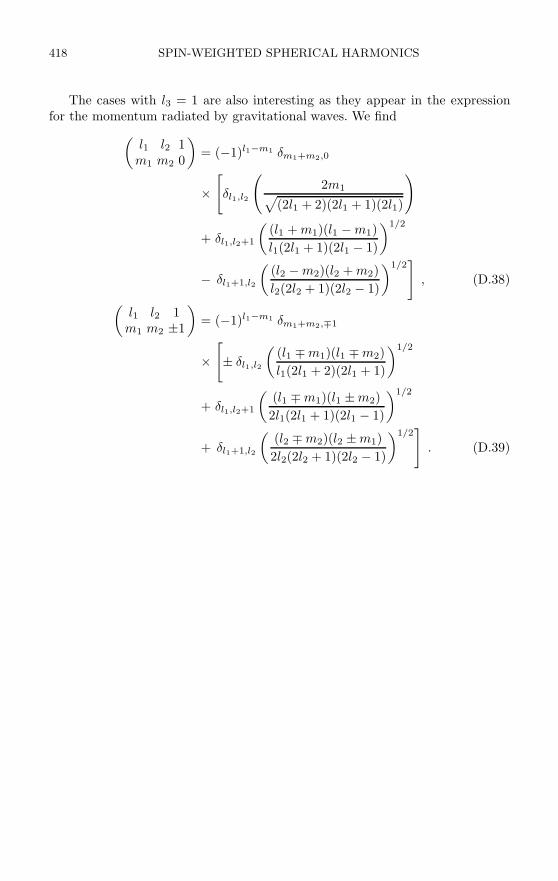
418 SPIN-WEIGHTED SPHERICAL HARMONICS
The cases with l3 = 1 are also interesting as they appear in the expressionfor the momentum radiated by gravitational waves. We find(
l1 l2 1m1 m2 0
)= (−1)l1−m1 δm1+m2,0
×[δl1,l2
(2m1√
(2l1 + 2)(2l1 + 1)(2l1)
)
+ δl1,l2+1
((l1 + m1)(l1 − m1)l1(2l1 + 1)(2l1 − 1)
)1/2− δl1+1,l2
((l2 − m2)(l2 + m2)l2(2l2 + 1)(2l2 − 1)
)1/2], (D.38)(
l1 l2 1m1 m2 ±1
)= (−1)l1−m1 δm1+m2,∓1
×[± δl1,l2
((l1 ∓ m1)(l1 ∓ m2)l1(2l1 + 2)(2l1 + 1)
)1/2+ δl1,l2+1
((l1 ∓ m1)(l1 ± m2)2l1(2l1 + 1)(2l1 − 1)
)1/2+ δl1+1,l2
((l2 ∓ m2)(l2 ± m1)2l2(2l2 + 1)(2l2 − 1)
)1/2]. (D.39)

REFERENCES
[1] Abrahams, A., Anderson, A., Choquet-Bruhat, Y., and York, J. Einstein andYang-Mills theories in hyperbolic form without gauge-fixing. Phys. Rev.Lett., 75:3377–3381, 1995.
[2] Alcubierre, M. The appearance of coordinate shocks in hyperbolic formulationsof general relativity. Phys. Rev. D, 55:5981–5991, 1997.
[3] Alcubierre, M. Hyperbolic slicings of spacetime: singularity avoidance and gaugeshocks. Class. Quantum Grav., 20(4):607–624, 2003.
[4] Alcubierre, M. Are gauge shocks really shocks? Class. Quantum Grav., 22:4071–4082, 2005.
[5] Alcubierre, M., Allen, G., Brugmann, B., Lanfermann, G., Seidel, E., Suen,W.-M., and Tobias, M. Gravitational collapse of gravitational waves in 3Dnumerical relativity. Phys. Rev. D, 61:041501 (R), 2000.
[6] Alcubierre, M., Allen, G., Brugmann, B., Seidel, E., and Suen, W.-M. Towardsan understanding of the stability properties of the 3+1 evolution equationsin general relativity. Phys. Rev. D, 62:124011, 2000.
[7] Alcubierre, M., Benger, W., Brugmann, B., Lanfermann, G., Nerger, L., Seidel,E., and Takahashi, R. 3D Grazing Collision of Two Black Holes. Phys. Rev.Lett., 87:271103, 2001.
[8] Alcubierre, M., Brandt, S. R., Brugmann, B., Gundlach, C., Masso, J., Seidel,E., and Walker, P. Test-beds and applications for apparent horizon findersin numerical relativity. Class. Quantum Grav., 17:2159–2190, 2000.
[9] Alcubierre, M., Brandt, S. R., Brugmann, B., Holz, D., Seidel, E., Takahashi,R., and Thornburg, J. Symmetry without symmetry: Numerical simula-tion of axisymmetric systems using Cartesian grids. Int. J. Mod. Phys. D,10(3):273–289, 2001.
[10] Alcubierre, M. and Brugmann, B. Simple excision of a black hole in 3+1numerical relativity. Phys. Rev. D, 63:104006, 2001.
[11] Alcubierre, M., Brugmann, B., Diener, P., Guzman, F. S., Hawke, I., Hawley,S., Herrmann, F., Koppitz, M., Pollney, D., Seidel, E., and Thornburg, J.Dynamical evolution of quasi-circular binary black hole data. Phys. Rev. D,72(4):044004, 2005.
[12] Alcubierre, M., Brugmann, B., Diener, P., Guzman, F. S., Hawke, I., Hawley,S., Herrmann, F., Koppitz, M., Pollney, D., Seidel, E., and Thornburg, J.Dynamical evolution of quasi-circular binary black hole data. Phys. Rev. D,72:044004, 5 August 2005.
[13] Alcubierre, M., Brugmann, B., Diener, P., Koppitz, M., Pollney, D., Seidel, E.,and Takahashi, R. Gauge conditions for long-term numerical black holeevolutions without excision. Phys. Rev. D, 67:084023, 2003.
419
420 REFERENCES
[14] Alcubierre, M., Brugmann, B., Dramlitsch, T., Font, J. A., Papadopoulos, P.,Seidel, E., Stergioulas, N., and Takahashi, R. Towards a stable numericalevolution of strongly gravitating systems in general relativity: The conformaltreatments. Phys. Rev. D, 62:044034, 2000.
[15] Alcubierre, M., Brugmann, B., Pollney, D., Seidel, E., and Takahashi, R. Blackhole excision for dynamic black holes. Phys. Rev. D, 64:061501(R), 2001.
[16] Alcubierre, M., Corichi, A., Gonzalez, J. A., Nunez, D., Reimann, B., and Sal-gado, M. Generalized harmonic spatial coordinates and hyperbolic shiftconditions. Phys. Rev. D, 72:124018, 2005.
[17] Alcubierre, M., Corichi, A., Gonzalez, J. A., Nunez, D., and Salgado, M. Ahyperbolic slicing condition adapted to killing fields and densitized lapses.Class. Quantum Grav., 20(18):3951–3968, 21 September 2003.
[18] Alcubierre, M. and Gonzalez, J. A. Regularization of spherically symmetricevolution codes in numerical relativity. Comp. Phys. Comm., 167:76–84,2005. gr-qc/0401113.
[19] Alcubierre, M. and Masso, J. Pathologies of hyperbolic gauges in general rela-tivity and other field theories. Phys. Rev. D, 57(8):R4511–R4515, 1998.
[20] Alcubierre, M. and Schutz, B. Time–symmetric ADI and causal reconnection:Stable numerical techniques for hyperbolic systems on moving grids. J.Comput. Phys., 112:44, 1994.
[21] Anderson, A. and York, J. W. Fixing Einstein’s equations. Phy. Rev. Lett.,82:4384–4387, 1999.
[22] Anderson, A. and York, J. W. Hamiltonian time evolution for general relativity.Phys. Rev. Lett., 81:1154–1157, 1998.
[23] Anninos, P., Bernstein, D., Brandt, S., Libson, J., Masso, J., Seidel, E., Smarr,L., Suen, W.-M., and Walker, P. Dynamics of apparent and event horizons.Phys. Rev. Lett., 74(5):630–633, 30 January 1995.
[24] Anninos, P., Brandt, S. R., and Walker, P. New coordinate systems for axisym-metric black hole collisions. Phys. Rev. D, 57:6158–6167, 1998.
[25] Anninos, P., Camarda, K., Masso, J., Seidel, E., Suen, W.-M., and Towns, J.Three-dimensional numerical relativity: The evolution of black holes. Phys.Rev. D, 52(4):2059–2082, 1995.
[26] Anninos, P., Daues, G., Masso, J., Seidel, E., and Suen, W.-M. Horizon bound-ary conditions for black hole spacetimes. Phys. Rev. D, 51(10):5562–5578,1995.
[27] Anninos, P., Hobill, D., Seidel, E., Smarr, L., and Suen, W.-M. The collisionof two black holes. Phys. Rev. Lett., 71(18):2851–2854, 1993.
[28] Anninos, P., Hobill, D., Seidel, E., Smarr, L., and Suen, W.-M. The head-oncollision of two equal mass black holes. Phys. Rev. D, 52:2044–2058, 1995.
[29] Arbona, A. and Bona, C. Dealing with the center and boundary problemsin 1d numerical relativity. Comput. Phys. Commun., 118:229–235, 1999.gr-qc/9805084.
[30] Arbona, A., Bona, C., Masso, J., and Stela, J. Robust evolution system fornumerical relativity. Phys. Rev. D, 60:104014, 1999. gr-qc/9902053.

REFERENCES 421
[31] Arnowitt, R., Deser, S., and Misner, C. W. The dynamics of general relativity.In Witten, L., editor, Gravitation: An introduction to current research, pages227–265. John Wiley, New York, 1962.
[32] Ashtekar, A., Beetle, C., Dreyer, O., Fairhurst, S., Krishnan, B., Lewandowski,J., and Wisniewski, J. Generic isolated horizons and their applications.Phys. Rev. Lett., 85:3564–3567, 2000.
[33] Ashtekar, A., Beetle, C., and Fairhurst, S. Isolated horizons: A generalizationof black hole mechanics. Class. Quantum Grav., 16:L1–L7, 1999.
[34] Ashtekar, A., Beetle, C., and Fairhurst, S. Mechanics of isolated horizons. Class.Quantum Grav., 17:253–298, 2000.
[35] Ashtekar, A., Fairhurst, S., and Krishnan, B. Isolated horizons: Hamiltonianevolution and the first law. Phys. Rev. D, 62:104025, 2000.
[36] Ashtekar, A. and Galloway, G. Some uniqueness results for dynamical horizons.Advances in Theoretical and Mathematical Physics, 9(1):1–30, 2005.
[37] Ashtekar, A. and Krishnan, B. Dynamical Horizons: Energy, angular momen-tum, fluxes, and balance laws. Phys. Rev. Lett., 89:261101, 2002.
[38] Ashtekar, A. and Krishnan, B. Dynamical horizons and their properties. Phys.Rev. D, 68:104030, 2003.
[39] Ashtekar, A. and Krishnan, B. Isolated and dynamical horizons and theirapplications. Living Rev. Relativity, 7:10, 2004.
[40] Babiuc, M. C., Szilagyi, B., and J.Winicour. Harmonic initial-boundary evolu-tion in general relativity. Phys. Rev. D, 73:064017, 2006.
[41] Baker, J. and Campanelli, M. Making use of geometrical invariants in blackhole collisions. Phys. Rev. D, 62:127501, 2000.
[42] Baker, J., Brugmann, B., Campanelli, M., Lousto, C. O., and Takahashi, R.Plunge waveforms from inspiralling binary black holes. Phys. Rev. Lett.,87:121103, 2001.
[43] Baker, J., Campanelli, M., Lousto, C. O., and Takahashi, R. Modeling gravita-tional radiation from coalescing binary black holes. Phys. Rev. D, 65:124012,2002.
[44] Baker, J. G., Centrella, J., Choi, D.-I., Koppitz, M., and van Meter, J. Binaryblack hole merger dynamics and waveforms. Phys. Rev. D, 73:104002, 2006.
[45] Baker, J. G., Centrella, J., Choi, D.-I., Koppitz, M., and van Meter, J. Gravi-tational wave extraction from an inspiraling configuration of merging blackholes. Phys. Rev. Lett., 96:111102, 2006.
[46] Balakrishna, J., Daues, G., Seidel, E., Suen, W.-M., Tobias, M., and Wang,E. Coordinate conditions in three-dimensional numerical relativity. Class.Quantum Grav., 13:L135–L142, 1996.
[47] Barcelo, C. and Visser, M. Twilight for the energy conditions? Int. J. Mod.Phys. D, 11:1553–1560, 2002.
[48] Bardeen, J. M. and Piran, T. General relativistic axisymmetric rotating sys-tems: Coordinates and equations. Phys. Reports, 196:205–250, 1983.
[49] Baumgarte, T. W. Innermost stable circular orbit of binary black holes. Phys.Rev. D, 62:024018, 2000.

422 REFERENCES
[50] Baumgarte, T. W. and Shapiro, S. L. On the numerical integration of Einstein’sfield equations. Phys. Rev. D, 59:024007, 1999.
[51] Beig, R. and Murchadha, N. O. Late time behavior of the maximal slicingof the Schwarzschild black hole. Phys. Rev. D, 57(8):4728–4737, 1998. gr-qc/9706046.
[52] Beig, R. The maximal slicing of a Schwarzschild black hole. Ann. Phys.,11(5):507–510, 2000.
[53] Belinski, V., Khalatnikov, I., and Lifshitz, E. Oscillatory approach to a singularpoint in the relativistic cosmology. Adv. Phys., 19:525–573, 1970.
[54] Bernstein, D. A Numerical Study of the Black Hole Plus Brill Wave Spacetime.PhD thesis, University of Illinois Urbana-Champaign, 1993.
[55] Bernstein, D., Hobill, D., and Smarr, L. Black hole spacetimes: Testing numer-ical relativity. In Evans, C., Finn, L., and Hobill, D., editors, Frontiers inNumerical Relativity, pages 57–73. Cambridge University Press, Cambridge,England, 1989.
[56] Bishop, N. T. The closed trapped region and the apparent horizon of twoSchwarzschild black holes. Gen. Rel. Grav., 14(9):717–723, 1982.
[57] Bishop, N. T. Numerical relativity: Combining the Cauchy and characteristicinitial value problem. Class. Quantum Grav., 10:333–341, 1993.
[58] Bishop, N. T., Isaacson, R., Maharaj, M., and Winicour, J. Black hole data viaa Kerr-Schild approach. Phys. Rev. D, 57:6113–6118, 1998.
[59] Bona, C., Ledvinka, T., Palenzuela, C., and Zacek, M. General-covariant evo-lution formalism for numerical relativity. Phys. Rev. D, 67:104005, 2003.
[60] Bona, C., Ledvinka, T., Palenzuela, C., and Zacek, M. A symmetry-breakingmechanism for the Z4 general-covariant evolution system. Phys. Rev. D,69:064036, 2004.
[61] Bona, C., Ledvinka, T., Palenzuela-Luque, C., and Zacek, M. Constraint-preserving boundary conditions in the Z4 numerical relativity formalism.Class. Quantum Grav., 22:2615–2634, 2005.
[62] Bona, C. and Masso, J. Einstein’s evolution equations as a system of balancelaws. Phys. Rev. D, 40(4):1022–1026, 1989.
[63] Bona, C. and Masso, J. Hyperbolic evolution system for numerical relativity.Phys. Rev. Lett., 68:1097, 1992.
[64] Bona, C. and Masso, J. Numerical relativity: evolving space-time. InternationalJournal of Modern Physics C: Physics and Computers, 4:883, 1993.
[65] Bona, C., Masso, J., Seidel, E., and Stela, J. New Formalism for NumericalRelativity. Phys. Rev. Lett., 75:600–603, 1995.
[66] Bona, C., Masso, J., Seidel, E., and Stela, J. First order hyperbolic formalismfor numerical relativity. Phys. Rev. D, 56:3405–3415, 1997.
[67] Bona, C. and Palenzuela, C. Dynamical shift conditions for the Z4 and BSSNhyperbolic formalisms. Phys. Rev. D, 69:104003, 2004.
[68] Bona, C. and Palenzuela-Luque, C. Elements of Numerical Relativity. Springer-Verlag, Berlin, 2005.
REFERENCES 423
[69] Bonazzola, S. and Gourgoulhon, E. A formulation of the virial theorem ingeneral relativity. Class. Quantum Grav., 11:1775–1784, 1994.
[70] Bonazzola, S. and Marck, J.-A. Pseudo-spectral methods applied to gravita-tional collapse. In Evans, C., Finn, L., and Hobill, D., editors, Frontiersin Numerical Relativity, pages 239–253. Cambridge University Press, Cam-bridge, England, 1989.
[71] Bondi, H., van der Burg, M. G. J., and Metzner, A. W. K. Gravitational wavesin general relativity VII. Waves from axi-symmetric isolated systems. Proc.R. Soc. London, A269:21–52, 1962.
[72] Booth, I. and Fairhurst, S. Horizon energy and angular momentum from ahamiltonian perspective. Class. Quantum Grav., 22:4515–4550, 2005.
[73] Bowen, J. M. General form for the longitudinal momentum of a sphericallysymmetric source. Gen. Rel. Grav., 11(3):227–231, 1979.
[74] Bowen, J. M. and York, J. W. Time-asymmetric initial data for black holesand black hole collisions. Phys. Rev. D, 21(8):2047–2056, 1980.
[75] Boyd, J. P. Chebyshev and Fourier Spectral Methods (Second Edition, Revised).Dover Publications, New York, 2001.
[76] Brandt, S. and Brugmann, B. A simple construction of initial data for multipleblack holes. Phys. Rev. Lett., 78(19):3606–3609, 1997.
[77] Brandt, S. and Seidel, E. The evolution of distorted rotating black holes III:Initial data. Phys. Rev. D, 54(2):1403–1416, 1996.
[78] Brill, D. S. On the positive definite mass of the Bondi-Weber-Wheeler time-symmetric gravitational waves. Ann. Phys. (N. Y.), 7:466–483, 1959.
[79] Brill, D. S. and Lindquist, R. W. Interaction energy in geometrostatics. Phys.Rev., 131(1):471–476, 1963.
[80] Brugmann, Bernd, Tichy, Wolfgang, Jansen, and Nina. Numerical simulationof orbiting black holes. Phys. Rev. Lett., 92:211101, 2004.
[81] Brugmann, B. Adaptive mesh and geodesically sliced Schwarzschild spacetimein 3+1 dimensions. Phys. Rev. D, 54(12):7361–7372, 1996.
[82] Brugmann, B. Binary black hole mergers in 3D numerical relativity. Int. J.Mod. Phys. D, 8:85, 1999.
[83] Brugmann, B., Gonzalez, J. A., Hannam, M., Husa, S., Sperhake, U., and Tichy,W. Calibration of moving puncture simulations. 2006. gr-qc/0610128.
[84] Bruhat, Y. Theoreme d’existence pour certains systemes d’equations aux de-rivees partielles non lineaires. Acta Mathematica, 88:141–225, 1952.
[85] Cadez, A. Colliding Black Holes. PhD thesis, University of North Carolina atChapel Hill, Chapel Hill, North Carolina, 1971.
[86] Cadez, A. Apparent horizons in the two-black-hole problem. Ann. Phys.,83:449–457, 1974.
[87] Calabrese, G., Lehner, L., and Tiglio, M. Constraint-preserving boundary con-ditions in numerical relativity. Phys. Rev. D, 65:104031, 2002.
[88] Calabrese, G., Pullin, J., Reula, O., Sarbach, O., and Tiglio, M. Well posedconstraint-preserving boundary conditions for the linearized Einstein equa-tions. Communications in Mathematical Physics, 240:377–395, 2003.
424 REFERENCES
[89] Calabrese, G. and Sarbach, O. Detecting ill posed boundary conditions ingeneral relativity. J. Math. Phys, 44:3888–3889, 2003.
[90] Campanelli, M. and Lousto, C. O. Second order gauge invariant gravitationalperturbations of a Kerr black hole. Phys. Rev. D, 59:124022, 1999.
[91] Campanelli, M., Kelly, B. J., and Lousto, C. O. The Lazarus project II: Space-like extraction with the quasi-Kinnersley tetrad. Phys. Rev. D, 73:064005,2006.
[92] Campanelli, M., Lousto, C. O., and Zlochower, Y. The last orbit of binaryblack holes. Phys. Rev. D, 73:061501(R), 2006.
[93] Campanelli, M., Lousto, C. O., Marronetti, P., and Zlochower, Y. Accurateevolutions of orbiting black-hole binaries without excision. Phys. Rev. Lett.,96:111101, 2006.
[94] Campanelli, M., Lousto, C. O., Zlochower, Y., Krishnan, B., and Merritt,D. Spin flips and precession in black-hole-binary mergers. Phys. Rev.,D75:064030, 2007.
[95] Caudill, M., Cook, G. B., Grigsby, J. D., and Pfeiffer, H. P. Circular orbits andspin in black-hole initial data. Phys. Rev. D, 74:064011, 2006.
[96] Chandrasekhar, S. The Mathematical Theory of Black Holes. Oxford UniversityPress, Oxford, England, 1983.
[97] Choptuik, M. W. Consistency of finite-difference solutions to Einstein’s equa-tions. Phys. Rev. D, 44:3124–3135, 1991.
[98] Choptuik, M. W. Universality and scaling in gravitational collapse of masslessscalar field. Phys. Rev. Lett., 70:9, 1993.
[99] Choptuik, M. W., Hirschmann, E. W., Liebling, S. L., and Pretorius, F. Anaxisymmetric gravitational collapse code. Class. Quantum Grav., 20:1857–1878, 2003.
[100] Choquet-Bruhat, Y. and York, J. Geometrical well posed systems for theEinstein equations. C. R. Acad. Sc. Paris, 321:1089, 1995.
[101] Cook, G. B. Three-dimensional initial data for the collision of two blackholes II: Quasi-circular orbits for equal-mass black holes. Phys. Rev. D,50(8):5025–5032, 1994.
[102] Cook, G. B. Initial data for numerical relativity. Living Rev. Relativity, 3:5,2000.
[103] Cook, G. B. Corotating and irrotational binary black holes in quasi-circularorbits. Phys. Rev. D, 65:084003, 2002.
[104] Cook, G. B., Huq, M. F., Klasky, S. A., Scheel, M. A., Abrahams, A. M.,Anderson, A., Anninos, P., Baumgarte, T. W., Bishop, N., Brandt, S. R.,Browne, J. C., Camarda, K., Choptuik, M. W., Correll, R. R., Evans, C. R.,Finn, L. S., Fox, G. C., Gomez, R., Haupt, T., Kidder, L. E., Laguna, P.,Landry, W., Lehner, L., Lenaghan, J., Marsa, R. L., Masso, J., Matzner,R. A., Mitra, S., Papadopoulos, P., Parashar, M., Rezzolla, L., Rupright,M. E., Saied, F., Saylor, P. E., Seidel, E., Shapiro, S. L., Shoemaker, D.,Smarr, L., Suen, W. M., Szilagyi, B., Teukolsky, S. A., van Putten, M.H. P. M., Walker, P., Winicour, J., and York Jr, J. W. Boosted three-

REFERENCES 425
dimensional black-hole evolutions with singularity excision. Phys. Rev. Lett.,80:2512–2516, 1998.
[105] Courant, R. and Friedrichs, K. O. Supersonic flows and shock waves. Springer,Berlin, 1976.
[106] Dain, S., Lousto, C. O., and Takahashi, R. New conformally flat initial datafor spinning black holes. Phys. Rev. D, 65:104038, 2002.
[107] Daues, G. E. Numerical Studies of Black Hole Spacetimes. PhD thesis, Wash-ington University, St. Louis, Missouri, 1996.
[108] de Felice, F. and Clarke, C. J. S. Relativity on curved manifolds. CambridgeUniversity Press, 1990.
[109] Diener, P. A new general purpose event horizon finder for 3D numerical space-times. Class. Quantum Grav., 20(22):4901–4917, 2003.
[110] Diener, P., Herrmann, F., Pollney, D., Schnetter, E., Seidel, E., Takahashi, R.,Thornburg, J., and Ventrella, J. Accurate evolution of orbiting binary blackholes. Phys. Rev. Lett., 96:121101, 2006.
[111] Dirac, P. A. M. Fixation of coordinates in the hamiltonian theory of gravita-tion. Phys. Rev., 114:924, 1959.
[112] Dray, T. The relationship between monopole harmonics and spin-weightedspherical harmonics. J. Math. Phys., 26:1030–1033, 1985.
[113] Dreyer, O., Krishnan, B., Shoemaker, D., and Schnetter, E. Introduction toIsolated Horizons in Numerical Relativity. Phys. Rev. D, 67:024018, 2003.
[114] Duez, M. D., Marronetti, P., Shapiro, S. L., and Baumgarte, T. W. Hydro-dynamic simulations in 3+1 general relativity. Phys. Rev. D, 67:024004,2003.
[115] Eardley, D. M. and Smarr, L. Time functions in numerical relativity:Marginally bound dust collapse. Phys. Rev. D, 19:2239, 1979.
[116] Eckart, C. The thermodynamics of irreversible processes III: Relativistic the-ory of the simple fluid. Phys. Rev., 58:919, 1940.
[117] Eddington, A. S. A comparison of Whitehead’s and Einstein’s formulas. Na-ture, 113:192, 1924.
[118] Einstein, A. Ist die tragheit eines korpers von seinem energieinhalt abhangig?Ann. Phys., 18:639–641, 1905.
[119] Einstein, A. Zur elektrodynamik bewegter korper. Ann. Phys., 17:891–921,1905.
[120] Einstein, A. Die feldgleichungen der gravitation. Preuss. Akad. Wiss. Berlin,Sitzungsber., pages 844–847, 1915.
[121] Einstein, A. Zur algemeinen relativitatstheorie. Preuss. Akad. Wiss. Berlin,Sitzungsber., pages 778–786, 1915.
[122] Emden, R. Gaskugeln, Anwendungen der mechanischen Warmetheorie. Teub-ner, Leipzig, 1907.
[123] Eppley, K. R. The numerical evolution of the collision of two black holes. PhDthesis, Princeton University, Princeton, New Jersey, 1975.
[124] Eppley, K. R. Evolution of time-symmetric gravitational waves: Initial dataand apparent horizons. Phys. Rev. D, 16(6):1609–1614, 1977.

426 REFERENCES
[125] Eppley, K. R. Pure gravitational waves. In Smarr, L., editor, Sources ofgravitational radiation, page 275. Cambridge University Press, Cambridge,England, 1979.
[126] Estabrook, F., Wahlquist, H., Christensen, S., DeWitt, B., Smarr, L., andTsiang, E. Maximally slicing a black hole. Phys. Rev. D, 7(10):2814–2817,1973.
[127] Evans, C. An approach for calculating axisymmetric gravitational collapse. InCentrella, J., editor, Dynamical Spacetimes and Numerical Relativity, pages3–39. Cambridge University Press, Cambridge, England, 1986.
[128] Finkelstein, D. Past-future asymmetry of the gravitational field of a pointparticle. Phys. Rev., 110:965–967, 1958.
[129] Font, J. A. Numerical hydrodynamics in general relativity. Living Rev. Rela-tivity, 6:4, 2003.
[130] Font, J., Ibanez, J., Martı, J., and Marquina, A. Multidimensional relativis-tic hydrodynamics: Characteristic fields and modern high-resolution shock-capturing schemes. Astron. Astrophys., 282:304, 1994.
[131] Friedrich, H. Hyperbolic reductions for Einstein’s equations. Class. QuantumGrav., 13:1451–1469, 1996.
[132] Friedrich, H. Conformal Einstein evolution. Lect. Notes Phys., 604:1–50, 2002.[133] Friedrich, H. and Nagy, G. The initial boundary value problem for Einstein’s
vacuum field equations. Commun. Math. Phys., 201:619–655, 1999.[134] Friedrichs, K. O. On the laws of relativistic electromagneto-fluid dynamics.
Commun. Pure Appl. Math., 27:749–808, 1974.[135] Frittelli, S. and Reula, O. First-order symmetric-hyperbolic Einstein equations
with arbitrary fixed gauge. Phys. Rev. Lett., 76:4667–4670, 1996.[136] Frittelli, S. Note on the propagation of the constraints in standard 3+1 general
relativity. Phys. Rev. D, 55:5992–5996, 1997.[137] Frittelli, S. and Gomez, R. Einstein boundary conditions for the Einstein equa-
tions in the conformal-traceless decomposition. Phys. Rev. D, 70:064008,2004.
[138] Frittelli, S. and Gomez, R. Einstein boundary conditions in relation to con-straint propagation for the initial-boundary value problem of the Einsteinequations. Phys. Rev. D, 69:124020, 2004.
[139] Garat, A. and Price, R. H. Nonexistence of conformally flat slices of the Kerrspacetime. Phys. Rev. D, 61:124011, 2000.
[140] Garfinkle, D. Harmonic coordinate method for simulating generic singularities.Phys. Rev. D, 65:044029, 2002.
[141] Garfinkle, D., Gundlach, C., and Hilditch, D. Comments on Bona-Masso typeslicing conditions in long-term black hole evolutions. 2007. arXiv:0707.0726.
[142] Gentle, A., Holz, D., Kheyfets, A., Laguna, P., Miller, W., and Shoemaker,D. Constant crunch coordinates for black hole simulations. Phys. Rev. D,63:064024, 2001.
[143] Gerlach, U. and Sengupta, U. Gauge-invariant perturbations on most generalspherically symmetric space-times. Phys. Rev. D., 19:2268–2272, 1979.

REFERENCES 427
[144] Geroch, R. A method for generating solutions of Einstein’s equations. J.Math. Phys., 12:918, 1971.
[145] Gleiser, R. J., Nicasio, C. O., Price, R. H., and Pullin, J. Evolving the Bowen-York initial data for spinning black holes. Phys. Rev. D, 57:3401–3407,1998.
[146] Godunov, S. K. A difference method for numerical calculations of discontinu-ous solutions of the equations of hydrpdynamics. Mat. Sb., 47:271, 1959. inRussian.
[147] Gomez, R., Lehner, L., Marsa, R., Winicour, J., Abrahams, A. M., Anderson,A., Anninos, P., Baumgarte, T. W., Bishop, N. T., Brandt, S. R., Browne,J. C., Camarda, K., Choptuik, M. W., Cook, G. B., Correll, R., Evans, C. R.,Finn, L. S., Fox, G. C., Haupt, T., Huq, M. F., Kidder, L. E., Klasky, S. A.,Laguna, P., Landry, W., Lenaghan, J., Masso, J., Matzner, R. A., Mitra, S.,Papadopoulos, P., Parashar, M., Rezzolla, L., Rupright, M. E., Saied, F.,Saylor, P. E., Scheel, M. A., Seidel, E., Shapiro, S. L., Shoemaker, D., Smarr,L., Szilagyi, B., Teukolsky, S. A., van Putten, M. H. P. M., Walker, P., andYork Jr, J. W. Stable characteristic evolution of generic three-dimensionalsingle-black-hole spacetimes. Phys. Rev. Lett., 80:3915–3918, 1998.
[148] Gourgoulhon, E. A generalized Damour-Navier-Stokes equation applied totrapping horizons. Phys. Rev., D72:104007, 2005.
[149] Gourgoulhon, E. and Jaramillo, J. L. A 3+1 perspective on null hypersurfacesand isolated horizons. Physics Reports, 423(4–5):159–294, February 2006.
[150] Grandclement, P., Gourgoulhon, E., and Bonazzola, S. Binary black holesin circular orbits. II. Numerical methods and first results. Phys. Rev. D,65:044021, 2002.
[151] Gundlach, C. and Walker, P. Causal differencing of flux-conservative equationsapplied to black hole spacetimes. Class. Quantum Grav., 16:991–1010, 1999.
[152] Gundlach, C. Pseudo-spectral apparent horizon finders: An efficient new al-gorithm. Phys. Rev. D, 57:863–875, 1998.
[153] Gundlach, C. Critical phenomena in gravitational collapse. Living Rev. Rela-tivity, 2:4, 1999.
[154] Gundlach, C. and Martin-Garcia, J. M. Symmetric hyperbolicity and consis-tent boundary conditions for second-order Einstein equations. Phys. Rev.D, 70:044032, 2004.
[155] Gundlach, C. and Martin-Garcia, J. M. Hyperbolicity of second-order in spacesystems of evolution equations. Class. Quantum Grav., 23:S387–S404, 2006.
[156] Gundlach, C. and Martin-Garcia, J. M. Well-posedness of formulations of theEinstein equations with dynamical lapse and shift conditions. Phys. Rev.D, 74:024016, 2006.
[157] Gustafsson, B., Kreiss, H.-O., and Oliger, J. Time dependent problems anddifference methods. Wiley, New York, 1995.
[158] Hahn, S. G. and Lindquist, R. W. The two body problem in geometrodynam-ics. Ann. Phys., 29:304–331, 1964.

428 REFERENCES
[159] Hannam, M., Husa, S., Pollney, D., Brugmann, B., and O’Murchadha, N.Geometry and regularity of moving punctures. Phys. Rev. Lett., 99:241102,2007.
[160] Hawking, S. W. The event horizon. In DeWitt, C. and DeWitt, B. S., editors,Black Holes, pages 1–55. Gordon and Breach, New York, 1973.
[161] Hawking, S. W. and Ellis, G. F. R. The large scale structure of spacetime.Cambridge University Press, Cambridge, England, 1973.
[162] Hayward, S. A. General laws of black hole dynamics. Phys. Rev. D,49(12):6467–6474, 15 June 1994.
[163] Holz, D., Miller, W., Wakano, M., and Wheeler, J. Coalescence of primalgravity waves to make cosmological mass without matter. In Hu, B. L. andJacobson, T. A., editors, Directions in General Relativity: Proceedings of the1993 International Symposium, Maryland; Papers in honor of Dieter Brill,page 339, Cambridge, England, 1993. Cambridge University Press.
[164] Hulse, R. and Taylor, J. Discovery of a pulsar in a binary system. Astrophys.J., 195:L51–L53, 1975.
[165] Husa, S. Numerical relativity with the conformal field equations. In Fernandez,L. and Gonzalez, L. M., editors, Proceedings of the 2001 spanish relativitymeeting, volume 617 of Lecture Notes in Physics, pages 159–192. Springer,2003.
[166] Isaacson, R. Gravitational radiation in the limit of high frequency. II. nonlinearterms and the effective stress tensor. Phys. Rev., 166:1272–1280, 1968.
[167] Israel, W. and Stewart, J. M. Transient relativistic thermodynamics and ki-netic theory. Ann. Phys., 118:341, 1979.
[168] Jantzen, R. T. and York, James W., J. New minimal distortion shift gauge.Phys. Rev. D, 73:104008, 2006.
[169] Katz, J. I., Lynden-Bell, D., and Israel, W. Quasilocal energy in static gravi-tational fields. Class. Quantum Grav., 5:971–987, 1988.
[170] Kerr, R. P. Gravitational field of a spinning mass as an example of algebraicallyspecial metrics. Phys. Rev. Lett., 11:237–238, 1963.
[171] Kidder, L. E. and Finn, L. S. Spectral methods for numerical relativity. theinitial data problem. Phys. Rev. D, 62:084026, 2000.
[172] Kidder, L. E., Scheel, M. A., and Teukolsky, S. A. Extending the lifetimeof 3D black hole computations with a new hyperbolic system of evolutionequations. Phys. Rev. D, 64:064017, 2001.
[173] Kidder, L. E., Scheel, M. A., Teukolsky, S. A., Carlson, E. D., and Cook, G. B.Black hole evolution by spectral methods. Phys. Rev. D, 62:084032, 2000.
[174] Kidder, L. E., Lindblom, L., Scheel, M. A., Buchman, L. T., and Pfeiffer,H. P. Boundary conditions for the Einstein evolution system. Phys. Rev.D, 71:064020, 2005.
[175] Kokkotas, K. D. and Schmidt, B. G. Quasi-normal modes of stars and blackholes. Living Rev. Relativity, 2:2, 1999. http://www.livingreviews.org/lrr-1999-2.

REFERENCES 429
[176] Komar, A. Covariant conservation laws in general relativity. Phys. Rev.,113:934–936, 1959.
[177] Kreiss, H. O. and Lorenz, J. Initial-boundary value problems and the Navier-Stokes equations. Academic Press, New York, 1989.
[178] Kreiss, H. O. and Oliger, J. Methods for the approximate solution of timedependent problems. GARP publication series No. 10, Geneva, 1973.
[179] Kreiss, H. O. and Scherer, G. Finite element and finite difference methods forhyperbolic partial differential equations. In Boor, C. D., editor, Mathemati-cal Aspects of Finite Elements in Partial Differential Equations, New York,1974. Academica Press.
[180] Kreiss, H. O. and Scherer, G. Method of lines for hyperbolic equations. SIAMJ. Numer. Anal., 29:640–646, 1992.
[181] Krishnan, B. Isolated Horizons in Numerical Relativity. PhD thesis, Pennsyl-vania State University, 2002.
[182] Kruskal, M. D. Maximal extension of Schwarzschild metric. Phys. Rev., pages1743–1745, 1960.
[183] Landau, L. D. and Lifshitz, E. M. The Classical Theory of Fields, Course ofTheoretical Physics, Volume 2. Elsevier Butterworth-Heinemann, Oxford,2004.
[184] Landau, L. D. and Lifshitz, E. M. Fluid Mechanics, Course of TheoreticalPhysics, Volume 6. Elsevier Butterworth-Heinemann, Oxford, 2004.
[185] Lax, P. D. and Phillips, R. S. Local boundary conditions for dissipative sym-metric linear differential operators. Commun. Pure Appl. Math., 13:427–455,1960.
[186] Lehner, L. Numerical relativity: A review. Class. Quantum Grav., 18:R25–R86, 2001.
[187] Leveque, R. J. Numerical Methods for Conservation Laws. Birkhauser Verlag,Basel, 1992.
[188] Libson, J., Masso, J., Seidel, E., Suen, W.-M., and Walker, P. Event horizonsin numerical relativity: Methods and tests. Phys. Rev. D, 53(8):4335–4350,1996.
[189] Lichnerowicz, A. L’integration des equations de la gravitation relativiste et laprobleme des n corps. J. Math. Pures et Appl., 23:37, 1944.
[190] Lindblom, L. and Scheel, M. A. Dynamical gauge conditions for the Einsteinevolution equations. Phys. Rev. D, 67:124005, 2003.
[191] Lindblom, L., Scheel, M. A., Kidder, L. E., Owen, R., and Rinne, O. A newgeneralized harmonic evolution system. Class. Quantum Grav., 23:S447–S462, 2006.
[192] Lindquist, R. W. Initial-value problem on Einstein-Rosen manifolds. Jour.Math. Phys., 4(7):938, 1963.
[193] Lousto, C. O. and Zlochower, Y. A practical formula for the radiated angularmomentum. Phys. Rev., D76:041502, 2007.
[194] Maartens, R. Dissipative cosmology. Class. Quantum Grav., 12:1455, 1995.
430 REFERENCES
[195] Maartens, R. Causal thermodynamics in relativity. Lectures given at theHanno Rund Workshop on Relativity and Thermodynamics, South Africa,June 1996; astro-ph/9609119, 1996.
[196] Marsa, R. L. and Choptuik, M. W. Black hole–scalar field interactions inspherical symmetry. Phys. Rev. D, 54:4929–4943, 1996.
[197] Martel, K. and Poisson, E. Gravitational perturbations of the schwarzschildspacetime: A practical covariant and gauge-invariant formalism. Phys. Rev.,D71:104003, 2005.
[198] Martı, J. M., Ibanez, J. M., and Miralles, J. M. Numerical relativistic hydro-dynamics: Local characteristic approach. Phys. Rev. D, 43:3794, 1991.
[199] Martı, J. M. and Muller, E. The analytical solution of the riemann problemin relativistic hydrodynamics. J. Fluid Mech., 258:317–333, 1994.
[200] Martı, J. M. and Muller, E. Numerical hydrodynamics in special relativity.Living Rev. Relativity, 6:7, 2003.
[201] Matzner, R. A., Huq, M. F., and Shoemaker, D. Initial data and coordinatesfor multiple black hole systems. Phys. Rev. D, 59:024015, 1999.
[202] Messiah, A. Quatum Mechanics. Dover Publications, New York, 1999.[203] Metzger, J. Numerical computation of constant mean curvature surfaces using
finite elements. Class. Quantum Grav., 21(19):4625–4646, 2004.[204] Misner, C. Wormhole initial conditions. Phys. Rev., 118(4):1110–1111, 1960.[205] Misner, C. W. The method of images in geometrostatics. Ann. Phys., 24:102–
117, 1963.[206] Misner, C. W., Thorne, K. S., and Wheeler, J. A. Gravitation. W. H. Freeman,
San Francisco, 1973.[207] Mitchell, A. R. The finite element method in partial differential equations. J.
Wiley and Sons, U.S.A., 1977.[208] Mitchell, A. R. and Griffiths, D. F. The Finite Difference Method in Partial
Differential Equations. Wiley, New York, 1980.[209] Moncrief, V. Gravitational perturbations of spherically symmetric systems. I.
the exterior problem. Annals of Physics, 88:323–342, 1974.[210] Moreno, C., Nunez, D., and Sarbach, O. Kerr-Schild type initial data for two
Kerr black holes. Class. Quantum Grav., 19:6059–6073, 2002.[211] Nagar, A. and Rezzolla, L. Gauge-invariant non-spherical metric perturbations
of schwarzschild black-hole spacetimes. Class. Quant. Grav., 22:R167, 2005.[212] Nagy, G., Ortiz, O. E., and Reula, O. A. Strongly hyperbolic second order
Einstein’s evolution equations. Phys. Rev. D, 70:044012, 2004.[213] Nakamura, T., Maeda, K., Miyama, S., and Sasaki, M. General Relativistic
Collapse of an Axially Symmetric Star. I —The Formulation and the InitialValue Equations—. Prog. Theor. Phys., 63:1229–1244, April 1980.
[214] Nakamura, T., Kojima, Y., and Oohara, K. A method of determining apparenthorizons in three-dimensional numerical relativity. Phys. Lett. A, 106(5-6):235–238, 10 December 1984.

REFERENCES 431
[215] Nakamura, T., Oohara, K., and Kojima, Y. General relativistic collapse toblack holes and gravitational waves from black holes. Prog. Theor. Phys.Suppl., 90:1–218, 1987.
[216] Nerozzi, A., Beetle, C., Bruni, M., Burko, L. M., and Pollney, D. Towardswave extraction in numerical relativity: The quasi-Kinnersley frame. Phys.Rev. D, 72:024014, 2005.
[217] Newman, E. T., Couch, E., Chinnapared, K., Exton, A., Prakash, A., andTorrence, R. Metric of a rotating charged mass. J. Math. Phys., 6(6):918–919, 1965.
[218] Newman, E. T. and Penrose, R. An approach to gravitational radiation by amethod of spin coefficients. J. Math. Phys., 3(3):566–578, 1962. erratum inJ. Math. Phys. 4, 998 (1963).
[219] Newman, E. T. and Penrose, R. Note on the Bondi-Metzner-Sachs group. J.Math. Phys., 7(5):863–870, May 1966.
[220] Newmann, J. V. and Richtmyer, R. D. A method for the numerical calculationof hydrodynamical shocks. J. Appl. Phys., 21:232, 1950.
[221] Nordstrom, G. On the energy of the gravitational field in Einstein’s theory.Proc. Kon. Ned. Akad. Wet., 20:1238–1245, 1918.
[222] O’Murchadha, N. and York, J. W. Gravitational energy. Phys. Rev. D,10(8):2345–2357, 1974.
[223] Pais, A. ’Subtle is the Lord...’ the science and the life of Albert Einsten. OxfordUniversity Press, Oxford and New York, 1982.
[224] Petrich, L. I., Shapiro, S. L., and Teukolsky, S. A. Oppenheimer-Snyder col-lapse with maximal time slicing and isotropic coordinates. Phys. Rev. D,31(10):2459–2469, 15 May 1985.
[225] Petrov, A. Z. Einstein Spaces. Pergamon Press, Oxford, 1969.[226] Pfeiffer, H. P. and York, J. W. Extrinsic curvature and the Einstein con-
straints. Phys. Rev. D, 67:044022, 2003.[227] Poisson, E. A Relativist’s Toolkit: The Mathematics of Black-Hole Mechanics.
Cambridge University Press, 2004.[228] Pollney, D. et al. Recoil velocities from equal-mass binary black-hole mergers:
a systematic investigation of spin-orbit aligned configurations. Phys. Rev.,D76:124002, 2007.
[229] Pons, J. A., Martı, J. M., and Muller, E. The exact solution of the Riemannproblem with non-zero tangential velocities in relativistic hydrodynamics.J. Fluid Mech., 422:125–139, 2000.
[230] Press, W. H., Flannery, B. P., Teukolsky, S. A., and Vetterling, W. T. Nu-merical Recipes. Cambridge University Press, New York, 2nd edition, 1992.
[231] Pretorius, F. Evolution of binary black hole spacetimes. Phys. Rev. Lett.,95:121101, 2005.
[232] Pretorius, F. Numerical relativity using a generalized harmonic decomposition.Class. Quantum Grav., 22:425–452, 2005.
[233] Pretorius, F. Simulation of binary black hole spacetimes with a harmonicevolution scheme. Class. Quantum Grav., 23:S529–S552, 2006.
432 REFERENCES
[234] Racah, G. Theory of complex spectra II. Phys. Rev., 62:438, 1942.[235] Regge, T. and Wheeler, J. Stability of a Schwarzschild singularity. Phys. Rev.,
108(4):1063–1069, 1957.[236] Reimann, B. Slice stretching at the event horizon when geodesically slicing
the Schwarzschild spacetime with excision. Class. Quantum Grav., 21:4297–4304, 2004.
[237] Reimann, B. How slice stretching arises when maximally slicing theSchwarzschild spacetime with vanishing shift. Class. Quantum Grav.,22:4563–4587, 2005.
[238] Reimann, B. and Brugmann, B. Late time analysis for maximal slicing ofreissner- nordstrom puncture evolutions. Phys. Rev. D, 69:124009, 2004.
[239] Reimann, B. and Brugmann, B. Maximal slicing for puncture evolutions ofSchwarzschild and Reissner-Nordstrom black holes. Phys. Rev. D, 69:044006,2004.
[240] Reissner, H. Uber die eigengravitationn des elektrischen felds nach der Ein-steinshen theorie. Ann. Phys., 50:106–120, 1916.
[241] Reula, O. Hyperbolic methods for Einstein’s equations. Living Rev. Relativity,1:3, 1998.
[242] Richardson, L. F. The approximate arithmetic solution by finite differences ofphysical problems involving differential equations, with applications to thestresses in a masonry dam. Phil. Trans. Roy. Soc., 210:307–357, 1910.
[243] Richtmyer, R. D. and Morton, K. Difference Methods for Initial Value Prob-lems. Interscience Publishers, New York, 1967.
[244] Rinne, O. and Stewart, J. M. A strongly hyperbolic and regular reduction ofEinstein’s equations for axisymmetric spacetimes. Class. Quantum Grav.,22:1143–11166, 2005.
[245] Ruiz, M., Alcubierre, M., and Nunez, D. Regularization of spherical and ax-isymmetric evolution codes in numerical relativity. Gen. Rel. Grav., 40:159–182, 2008.
[246] Ruiz, M., Takahashi, R., Alcubierre, M., and Nunez, D. Multipole ex-pansions for energy and momenta carried by gravitational waves. 2007.arXiv:0707.4654.
[247] Sachs, R. Gravitational waves in general relativity VIII. Waves in asymptot-ically flat space-time. Proc. Roy. Soc. London, A270:103–126, 1962.
[248] Salgado, M. General relativistic hydrodynamics: a new approach. Rev. Mex.Fis., 44:1–8, 1998.
[249] Sarbach, O., Calabrese, G., Pullin, J., and Tiglio, M. Hyperbolicity of theBSSN system of Einstein evolution equations. Phys. Rev. D, 66:064002,2002.
[250] Sarbach, O. and Tiglio, M. Exploiting gauge and constraint freedom in hyper-bolic formulations of Einstein’s equations. Phys. Rev. D, 66:064023, 2002.
[251] Sarbach, O. and Tiglio, M. Boundary conditions for Einstein’s field equa-tions: analytical and numerical analysis. Journal of Hyperbolic DifferentialEquations, 2:839–883, 2005.

REFERENCES 433
[252] Sarbach, O. and Tiglio, M. Gauge invariant perturbations of Schwarzschildblack holes in horizon-penetrating coordinates. Phys. Rev. D, 64:084016,2001.
[253] Scheel, M., Baumgarte, T., Cook, G., Shapiro, S. L., and Teukolsky, S. Nu-merical evolution of black holes with a hyperbolic formulation of generalrelativity. Phys. Rev. D, 56:6320–6335, 1997.
[254] Scheel, M. A., Baumgarte, T. W., Cook, G. B., Shapiro, S. L., and Teukol-sky, S. A. Treating instabilities in a hyperbolic formulation of Einstein’sequations. Phys. Rev. D, 58:044020, 1998.
[255] Scheel, M. A., Pfeiffer, H. P., Lindblom, L., Kidder, L. E., Rinne, O., andTeukolsky, S. A. Solving Einstein’s equations with dual coordinate frames.Phys. Rev. D, 74:104006, 2006.
[256] Scheel, M. A., Shapiro, S. L., and Teukolsky, S. A. Collapse to black holesin Brans-Dicke theory: I. horizon boundary conditions for dynamical space-times. Phys. Rev. D, 51(8):4208–4235, 1995.
[257] Schnetter, E., Diener, P., Dorband, N., and Tiglio, M. A multi-block infras-tructure for three-dimensional time-dependent numerical relativity. Class.Quantum Grav., 23:S553–S578, 2006.
[258] Schutz, B. F. Geometrical methods of mathematical physics. Cambridge Uni-versity Press, 1980.
[259] Schutz, B. F. A first course in general relativity. Cambridge University Press,1985.
[260] Schwarzschild, K. Uber das Gravitationsfeld eines Massenpunktes nach derEinsteinchen Theorie. Sitzungsber. Dtsch. Akad. Wiss. Berlin, Kl. Math.Phys. Tech., pages 189–196, 1916.
[261] Seidel, E. and Suen, W.-M. Towards a singularity-proof scheme in numericalrelativity. Phys. Rev. Lett., 69(13):1845–1848, 1992.
[262] Shapiro, S. L. and Teukolsky, S. A. Gravitational collapse of supermassive starsto black holes: Numerical solution of the Einstein equations. AstrophysicalJ., 234:L177–L181, December 15 1979.
[263] Shapiro, S. L. and Teukolsky, S. A. Gravitational collapse to neutron stars andblack holes: Computer generation of spherical spacetimes. Astrophysical J.,235:199–215, 1980.
[264] Shapiro, S. L. and Teukolsky, S. A. Black Holes, White Dwarfs, and NeutronStars. John Wiley & Sons, New York, 1983.
[265] Shapiro, S. L. and Teukolsky, S. A. Relativistic stellar dynamics on thecomputer. I. Motivation and numerical method. Astrophys. J., 298:34–57,November 1 1985.
[266] Shapiro, S. L. and Teukolsky, S. A. Relativistic stellar dynamics on the com-puter. II. Physical applications. Astrophys. J., 298:58–79, November 1 1985.
[267] Shibata, M. Time symmetric initial conditions of gravitational waves for 3Dnumerical relativity. Phys. Rev. D, 55:7529–7537, 1997.
[268] Shibata, M. and Nakamura, T. Evolution of three-dimensional gravitationalwaves: Harmonic slicing case. Phys. Rev. D, 52:5428, 1995.
434 REFERENCES
[269] Shoemaker, D. M., Huq, M. F., and Matzner, R. A. Generic tracking ofmultiple apparent horizons with level flow. Phys. Rev. D, 62:124005, 2000.
[270] Smarr, L. The Structure of General Relativity with a Numerical Illustration:The Collision of Two Black Holes. PhD thesis, University of Texas, Austin,Austin, Texas, 1975.
[271] Smarr, L., Cadez, A., DeWitt, B., and Eppley, K. R. Collision of two blackholes: Theoretical framework. Phys. Rev. D, 14(10):2443–2452, 1976.
[272] Smarr, L. and York, J. W. Kinematical conditions in the construction ofspacetime. Phys. Rev. D, 17(10):2529–2552, 15 May 1978.
[273] Smarr, L. and York, J. W. Radiation gauge in general relativity. Phys. Rev.D, 17:1945, 1978.
[274] Sopuerta, C. F., Yunes, N., and Laguna, P. Gravitational recoil from binaryblack hole mergers: The close-limit approximation. Phys. Rev., D74:124010,2006.
[275] Stergioulas, N. Rotating stars in relativity. Living Rev. Relativity, 6:3, 2003.[276] Szabados, L. B. Quasi-local energy-momentum and angular momentum in
general relativity: A review article. Living Reviews in Relativity, 7(4), 2004.[277] Szekeres, P. On the singularities of a Riemannian manifold. Publ. Mat. De-
brecen, 7:285–301, 1960.[278] Szilagyi, B., Gomez, R., Bishop, N. T., and Winicour, J. Cauchy boundaries
in linearized gravitational theory. Phys. Rev. D, 62:104006, 2000.[279] Szilagyi, B., Schmidt, B., and Winicour, J. Boundary conditions in linearized
harmonic gravity. Phys. Rev. D, 65:064015, 2002.[280] Szilagyi, B. and Winicour, J. Well-posed initial-boundary evolution in general
relativity. Phys. Rev. D, 68:041501, 2003.[281] Tadmor, E. Spectral methods for hyperbolic problems. In Lecture notes deliv-
ered at Ecole des Ondes, ”Methodes numeriques d’ordre eleve pour les ondesen regime transitoire”, INRIA–Rocquencourt January 24-28., 1994.
[282] Taylor, J. H. and Weisberg, J. M. A new test of general relativity: Grav-itational radiation and the binary pulsar PSR 1913+16. Astrophys. J.,253:908–920, 1982.
[283] Teukolsky, S. On the stability of the iterated crank-nicholson method in nu-merical relativity. Phys. Rev. D, 61:087501, 2000.
[284] Thornburg, J. Coordinates and boundary conditions for the general relativisticinitial data problem. Class. Quantum Grav., 4(5):1119–1131, September1987.
[285] Thornburg, J. Numerical Relativity in Black Hole Spacetimes. PhD thesis,University of British Columbia, Vancouver, British Columbia, 1993.
[286] Thornburg, J. A 3+1 computational scheme for dynamic spherically symmet-ric black hole spacetimes – II: Time evolution. gr-qc/9906022, 1999.
[287] Thornburg, J. Event and apparent horizon finders for 3+1 numerical relativity.Living Rev. Relativity, 2006. [Online article].
[288] Thorne, K. Multipole expansions of gravitational radiation. Rev. Mod. Phys.,52(2):299, 1980.
REFERENCES 435
[289] Tichy, W. and Brugmann, B. Quasi-equilibrium binary black hole sequencesfor puncture data derived from helical killing vector conditions. Phys. Rev.D, 69:024006, 2004.
[290] Tichy, W., Brugmann, B., and Laguna, P. Gauge conditions for binary blackhole puncture data based on an approximate helical Killing vector. Phys.Rev. D, 68:064008, 2003.
[291] Tod, K. P. Looking for marginally trapped surfaces. Class. Quantum Grav.,8:L115–L118, 1991.
[292] Toro, E. F. Riemann Solvers and Numerical Methods for Fluid Dynamics.Springer-Verlag, 1999.
[293] van Meter, J. R., Baker, J. G., Koppitz, M., and Choi, D.-I. How to move ablack hole without excision: gauge conditions for the numerical evolution ofa moving puncture. Phys. Rev. D, 73:124011, 2006.
[294] Varshalovich, D. A. and Kersonskii, V. K. Quatum theory of angular momen-tum. World Scientific, Singapore, 1989.
[295] Wald, R. M. General relativity. The University of Chicago Press, Chicago,1984.
[296] Walker, P. Horizons, Hyperbolic Systems, and Inner Boundary Conditionsin Numerical Relativity. PhD thesis, University of Illinois at Urbana-Champaign, Urbana, Illinois, 1998.
[297] Weinberg, S. Gravitation and Cosmology: Principles and Applications of theGeneral Theory of Relativity. John Wiley and Sons, New York, 1972.
[298] Wheeler, J. A. A journey into gravity and spacetime. Scientific AmericanLibrary, distributed by W. H. Freeman, New York, U.S.A., 1990.
[299] Wigner, E. P. Group theory and its applications to the quantum mechanics ofatomic spectra. Academic Press, New York, 1959.
[300] Wilson, J. R. and Mathews, G. J. Relativistic numerical hydrodynamics. Cam-bridge University Press, 2003.
[301] Winicour, J. Characteristic evolution and matching. Living Rev. Relativity,1:5, 1998. [Online article].
[302] Yo, H.-J., Baumgarte, T. W., and Shapiro, S. L. Improved numerical stabilityof stationary black hole evolution calculations. Phys. Rev. D, 66:084026,2002.
[303] York, J. W. Gravitational degrees of freedom and the initial-value problem.Phys. Rev. Lett., 26:1656–1658, 1971.
[304] York, J. W. Role of conformal three-geometry in the dynamics of gravitation.Phys. Rev. Lett., 28:1082–1085, 1972.
[305] York, J. W. Kinematics and dynamics of general relativity. In Smarr, L. L., ed-itor, Sources of gravitational radiation, pages 83–126. Cambridge UniversityPress, Cambridge, UK, 1979.
[306] York, J. W. Energy and momentum of the gravitational field. In Tipler, F. J.,editor, Essays in General Relativity: A Festschrift for Abraham Taub, pages39–58. Academic Press, New York, 1980.
436 REFERENCES
[307] York, J. W. Conformal ‘thin-sandwich’ data for the initial-value problem ofgeneral relativity. Phys. Rev. Lett., 82:1350–1353, 1999.
[308] Zerilli, F. J. Effective potential for even-parity Regge-Wheeler gravitationalperturbation equations. Phys. Rev. Lett., 24(13):737–738, 1970.
[309] Zerilli, F. J. Gravitational field of a particle falling in a Schwarzschild geometryanalyzed in tensor harmonics. Phys. Rev. D., 2:2141, 1970.

INDEX
(2 + 1) + 1 decomposition, 3911 + 1 equations, 3583 + 1 formalism, 654-acceleration, 1224-momentum, 304-velocity, 30, 122
accelerationequivalence principle, 1, 28in special relativity, 3of timelike curves, 141proper, 122tidal, 36
achronal set, 58action, 33adiabatic index, 253adiabatic process, 255, 258ADM
angular momentum, 110, 118, 236, 403equations, 75, 164, 357linear momentum, 110mass, 107, 113, 118, 152, 389, 403momentum, 403
advection equation, 152, 162, 335affine parameter, 23algebraically special spacetime, 300amplification matrix, 327angle
between vectors, 13Euler, 7solid, 19, 223, 309, 370
angular momentumADM, 110, 118, 236, 403conservation, 31flux in gravitational waves, 312, 316flux through horizon, 236Komar, 119, 406of isolated horizon, 235operators, 312, 415
angular velocity, 117, 119apparent horizon, 107
definition, 62, 221direct solvers, 229equation, 222flow algorithms, 227in axial symmetry, 225in Misner data, 109in spherical symmetry, 223, 371minimization algorithms, 226
areal radius, 47, 200, 371, 378artificial dissipation, 343, 386, 399artificial viscosity, 345asymptotic flatness, 48, 105, 111, 118,
126, 188, 402
bag of gold geometry, 47balance law, 162basis
coordinate, 8dual, 9null, 295orthonormal, 291transformation, 18
Bianchi identities, 28, 76, 195, 289bipolar coordinates, 204BKL conjecture, 140black hole
angular momentum, 55Bowen–York, 113definition, 61extremal, 55initial data, 105Kerr–Newman, 54, 113quasi-normal modes, 282Reissner–Nordstrom, 54Schwarzschild, 52
Boltzmann constant, 253Boltzmann equation, 252Bona–Masso
formulation, 169slicing, 135, 168, 171, 176, 210, 357, 375
Bondi mass, 407Bondi–Sachs coordinates, 89boundary conditions
absorbing, 332constraint preserving, 187, 194Dirichlet, 145, 194, 333maximally dissipative, 193, 196mixed, 333Newmann, 145, 194, 333outgoing-wave, 146, 333radiative, 188, 333Robin, 127, 379Sommerfeld, 188, 194well-posedness, 187
Bowen–York extrinsic curvature, 110, 120,207
Boyer–Lindquist coordinates, 56
437
438 INDEX
Brandt–Bruegmann initial data, 112Brill waves, 113
evolution, 397initial data, 395
Brill–Lindquist initial data, 107, 207, 220BSSNOK formulation, 82, 175, 207, 410Burgers’ equation, 148, 264, 361
Cadez coordinates, 204cartoon method, 399Cauchy
horizon, 58problem, 65, 75, 133, 156surface, 58
Cauchy-characteristic matching, 89, 187causal
curve, 58past and future, 57structure, 57
causal differencing, 215caustics, 88characteristic
fields, 160formalism, 87matrix, 158, 358speed, 147
chart, 7Christoffel symbols, 85
definition, 23difference as tensor, 24in 3+1 language, 409transformation, 24
chronological past and future, 58Clebsch–Gordan coefficients, 416co-vector, 9Codazzi–Mainardi equations, 72commutator, 16computational
domain, 324grid, 319stencil, 338
conformalconnection function, 83decomposition, 92diagram, 61factor, 13, 82, 90, 111flatness, 53, 96, 105, 113, 118, 207formalism, 90, 187infinity, 61Killing field, 94metric, 83, 90, 93, 101, 115, 142, 175thin-sandwich, 92transformation, 13, 82, 288
congruenceof null curves, 59
of timelike curves, 37, 70, 141connection coefficients, 21, 293conservation law, 162, 358conservative methods, 348consistency of difference approximations,
320, 385constant mean curvature, 96constrained evolution, 78constraint hypersurface, 76contact discontinuity, 267convergence of difference approximations,
321convergence testing, 354, 368coordinate singularity, 123, 200, 370, 385coordinates
bipolar, 204Cadez, 204corotating, 151, 209curvilinear, 150cylindrical, 391spherical, 19transformation, 17
cosmic censorship, 60Courant parameter, 323Courant–Friedrich–Lewy stability
condition, 153, 328covariance principle, 1, 29covariant derivative, 14, 21, 71Crank–Nicholson method, 338critical phenomena, 369, 390Cunningham–Price–Moncrief master
function, 283curvature
Ricci scalar, 27Ricci tensor, 27Riemann tensor, 26Weyl tensor, 288
curvecausal, 58definition, 8extremal, 23null, 7spacelike, 7timelike, 7
d’Alambertian operator, 36, 41derivative
covariant, 14, 21, 71intrinsic, 294Lie, 14, 74, 85operator, 20
difference operators, 325Dirac gauge, 143dispersion, 330dissipation, 330
INDEX 439
distortion tensor, 142domain of dependence, 58, 88dual
basis, 9tangent space, 9Weyl tensor, 289
dust, 252dynamical horizon, 236
Eddington–Finkelstein coordinates, 49,129
effective potential method, 116eigenfunctions, 160Einstein
equations, 37, 40, 71special relativity postulates, 2summation convention, 2tensor, 28
Einstein–Maxwell equations, 54Einstein–Rosen bridge, 52, 107, 111, 128,
201electrodynamics, 2electromagnetic field
Lagrangian, 35stress-energy tensor, 35
elliptic equation, 78, 89, 93, 95, 104, 124,143, 229, 395
energyconditions, 59conservation, 31constraint, 72density, 72, 92, 239flux in gravitational waves, 309, 313flux through horizon, 236of a particle, 30potential, 31, 116
entropy conditions, 267equation of state
dust, 252general, 241ideal gas, 252polytropic, 254
equivalence principle, 1, 28ergosphere, 55essentially non-oscillatory methods, 353Estabrook–Wahlquist time, 128Euler angles, 7Euler equations
in 3+1 language, 251, 260in general relativity, 248in special relativity, 241, 243Newtonian, 257
Euler method, 336Eulerian
frame, 238
observers, 66event horizon
definition, 52, 61finding, 230in Misner data, 109
expansionof null curves, 60, 222, 297of timelike curves, 141
explicit approximations, 323extrinsic curvature
as Lie derivative, 70Bowen–York, 110, 120, 207definition, 69tracefree, 83, 93
Fermi gas, 257finite differencing, 319finite elements, 318fluid
conservation laws, 241energy density, 239enthalpy, 239entropy, 244imperfect, 271internal energy, 239perfect, 239pressure, 239stress energy tensor, 32, 239, 271
flux limiter, 350flux vectors, 162foliation, 65
hyperboloidal, 90null, 88spacelike, 65, 122
p-forms, 8, 10free evolution, 78Friedmann–Robertson–Walker metric, 302
gaugeDirac, 143functions, 67, 73harmonic, 134, 149Lorentz, 41, 43pathology, 123, 369polar-areal, 371radiation, 141Regge–Wheeler, 282, 283shocks, 359speed, 135, 147, 171transformation, 41, 280transverse-traceless, 43, 284
Gauss–Codazzi equations, 72geodesic
definition, 23deviation, 37, 45

440 INDEX
in general relativity, 29in special relativity, 7slicing, 123, 209
geometric units, 2Gibbs phenomena, 346Godunov’s method, 348gradient
as a one-form, 10transformation, 18
gravitational radius, 48gravitational waves
angular momentum flux, 312, 316detectors, 46, 276energy flux, 309, 313linear momentum flux, 310, 315polarization, 45stress-energy pseudo-tensor, 306stress-energy tensor, 307tidal forces, 44weak field, 42
group velocity, 330
Hamilton’s equations, 81Hamiltonian constraint, 72, 75, 81, 92, 93,
123Hamiltonian formulation, 75, 79harmonic
coordinates, 134, 149slicing, 134, 140, 185
Hawking mass, 407heat conduction, 239, 272heat equation, 145, 156, 228, 273Helmholtz equation, 124Hermitian matrix, 159, 191high resolution methods, 350higher derivative formulations, 184Hilbert Lagrangian, 38, 78, 80hyperbolic
energy norm, 160globally hyperbolic spacetime, 58strictly hyperbolic, 160strongly hyperbolic, 135, 159, 172, 174,
177, 183, 187, 258, 262symmetric hyperbolic, 91, 159, 178, 185system, 82, 158, 261, 374weakly hyperbolic, 159, 167
ideal gas, 252, 259implicit approximations, 326index
co-variant and contra-variant, 18contraction, 9raising and lowering, 12
inertial framesdragging, 55, 392
global, 3local, 28
infinityconformal, 61null, 61spacelike, 61, 187timelike, 61
initial dataBrill–Lindquist, 107, 207, 220conformal decomposition, 92effective potential, 116isometric, 111Kerr–Schild, 114, 200Minkowski, 105Misner, 107, 200multiple black holes, 105punctures, 112quasi-circular, 115quasi-equilibrium, 117Schwarzschild, 106thin-sandwich, 92, 101, 117time-symmetric, 105
initial value problem, 65, 133, 156innermost stable circular orbit, 117intrinsic derivative, 294Isaacson stress-energy tensor, 307isolated horizon, 235isometry, 53, 107, 110, 201isotropic coordinates, 53, 106, 200, 224,
378isotropic lapse, 106, 202iterative Crank–Nicholson method, 341,
365, 380
Jordan block, 158jump conditions, 266
Kerr–Newman metric, 54, 302Kerr–Schild coordinates, 49, 56, 129, 232Kerr–Schild initial data, 114, 200Kidder–Scheel–Teukolsky formulation,
180Killing equation, 17, 25Killing field
axial, 119, 235conformal, 94, 142conserved quantities, 31definition, 17global energy and momentum, 405helical, 117
Klein–Gordonequation, 36, 384field, 35Lagrangian, 35stress-energy tensor, 35
INDEX 441
Komarangular momentum, 119, 406integral, 406mass, 118, 152, 406
Kreiss–Oliger dissipation, 343, 386, 399Kronecker delta, 9Kruskal diagram, 51, 128Kruskal–Szekeres coordinates, 51
Lagrangiandensity, 34, 80electromagnetic field, 35frame, 238general definition, 33Hilbert, 38, 78, 80Klein–Gordon field, 35
Laplaceequation, 97, 106, 145, 157operator, 86, 93, 105, 189, 278, 413
lapsecollapse, 125, 131, 137, 380, 389densitized, 81, 102, 134, 168, 185function, 66, 102, 118, 122pre-collapsed, 212, 218, 382
Lax equivalence theorem, 322Lax–Friedrichs method, 336Lax–Wendroff
method, 336theorem, 348
leapfrog method, 337Legendre polynomials, 413length
contraction, 6proper, 6
Levi–Civita tensor, 14, 289Lie
bracket, 16derivative, 14, 24, 70, 74, 85dragging, 15
light-cone, 5, 53light-cylinder, 153limiting surface, 125, 129, 210, 220linear degeneracy, 268local flatness, 27, 373, 393Lorentz
factor, 3gauge, 41, 43transformations, 3, 17, 18, 40
Lorentz–Fitzgerald contraction, 6
Mach number, 269Mach’s principle, 1, 55manifold
definition, 7local flatness, 27
symmetries, 16time orientable, 57
marginally trapped surface, 60mass
ADM, 107, 113, 118, 152, 389, 403bare, 107Bondi, 407Hawking, 407irreducible, 56, 116Komar, 118, 152, 406Newtonian, 390of isolated horizon, 236Schwarzschild-like, 389, 408
master functionCunningham–Price–Moncrief, 283Moncrief, 287Zerilli–Moncrief, 282
matterenergy density, 72, 92momentum density, 72, 92stress tensor, 74
maximal slicing, 109, 118, 123, 127, 210,379
Maxwell equations, 3, 73, 289method of lines, 339metric
conformal, 101, 115, 142, 175conformally flat, 96, 105, 207, 405Euclidean, 11in cylindrical coordinates, 392in spherical coordinates, 19, 46induced, 13, 67Lorentzian, 11mapping from vectors to one-forms, 11on the sphere, 19tensor, 11three-dimensional, 66
Michelson and Morley, 2minimal coupling, 29Minkowski metric, 4, 6, 90, 105, 231, 239,
302, 364minmod limiter, 351Misner initial data, 107, 200momentum
ADM, 110, 403canonical, 75, 80density, 72, 92flux in gravitational waves, 310, 315
momentum constraints, 73, 81, 86, 92, 93,109, 167
Moncrief master function, 287monotonicity preserving methods, 350multi-patch codes, 216multipole expansion, 278, 313
Nagy–Ortiz–Reula formulation, 172, 397

442 INDEX
Navier–Stokes equations, 273Newman–Penrose formalism, 294, 414Newton’s first law, 7, 29Newtonian
limit, 42potential, 31, 36, 42
non-expanding horizon, 234norm
energy norm, 160, 178, 191of a vector, 11of solutions, 156root mean square, 322
normal vector, 67, 110, 118, 192, 221null
curve, 7foliation, 88infinity, 61, 88principal directions, 300rotations, 297separation, 4surface, 230tetrad, 295vector, 11
Nyquist limit, 327, 344
one-formcovariant derivative, 21definition, 8transformation, 18
operatorangular momentum, 415d’Alambertian, 36, 41derivative, 20finite differencing, 325Laplace, 86, 93, 105, 189, 278, 413projection, 12, 59, 69, 141spin raising and lowering, 415
parabolic equation, 145, 273parallel transport, 22peeling theorem, 302Penrose process, 56Petrov classification, 299phase velocity, 330polytrope, 254pressure, 239principal null directions, 300principal symbol, 159projection operator, 12, 59, 69, 141punctures
evolution, 82, 206, 382initial data, 107, 112, 132, 152moving, 217
quantum gravity, 75
quasi-normal modes, 282
rarefaction waves, 266ray-body, 225Regge–Wheeler
equation, 284gauge, 282, 283
regularityand local flatness, 373in axial symmetry, 393in spherical symmetry, 371
Reissner–Nordstrom metric, 54relativity
general, 29principle, 2special, 2
relaxation time, 275Ricci
identity, 26rotation coefficients, 293scalar, 27, 79scalars, 298tensor, 27, 40, 85
Richardson’s extrapolation, 356Riemann problem, 265, 348Riemann tensor, 26, 72, 294
linearized, 40Roe’s limiter, 351Runge–Kutta methods, 340
scalarcurvature, 27function, 10product, 10
scalar fieldevolution, 386stress-energy tensor, 384
Schwarzschildcoordinates, 47evolution of, 378free fall time, 123free-fall time, 209metric, 48, 106, 127, 224, 302radius, 48
Schwarzschild perturbations, 277and Weyl scalar Ψ4, 308even, 280gauge invariant, 281, 283odd, 283TT gauge, 287
Schwarzschild-like mass, 389, 408shear of timelike curves, 141shift
driver conditions, 146gamma driver, 146, 213
INDEX 443
gamma freezing, 143harmonic, 149minimal distortion, 143, 212minimal strain, 142superluminal, 68, 215vector, 66, 102, 118, 140
shocksgauge shocks, 148, 359heating, 256in Burger’s equation, 264in hydrodynamics, 268shock avoiding gauge, 360, 363shock tube, 268shock wave, 266
short wavelength approximation, 307signature, 2simultaneity, 3singularity
focusing, 136naked, 55, 60ring, 55shell-crossing, 252theorems, 58
singularity avoidance, 124, 137, 209singularity excision, 126, 211, 214slice stretching, 126, 212, 380slicing condition
1+log, 135, 138, 210, 363, 382, 397Bona–Masso, 135, 168, 171, 176, 210,
357, 375geodesic, 123, 209harmonic, 134, 140, 185hyperbolic, 133maximal, 109, 118, 123, 127, 210, 379
slope limiter, 352, 365solution error, 320spacelike
curve, 7foliation, 65, 122infinity, 61, 187separation, 4vector, 11
spacetime invariants, 303speciality index, 304specific heat, 253spectral methods, 318spectral radius, 327speed of light
as maximum speed, 5coordinate, 49, 136geometric units, 2gravitational waves, 42invariance of, 3
speed of sound, 258, 262spherical harmonics, 278, 413
spherical symmetry, 370spin coefficients, 295spin raising and lowering operators, 415spin-boost transformations, 297spin-weighted harmonics, 279, 313, 414sponge filter, 333stability
CFL condition, 145, 153, 328, 338of difference approximations, 321of parabolic equations, 145von Newmann analysis, 326
static spacetime, 31stationary spacetime, 54strain
of timelike curves, 141tensor, 141
stress tensor, 74stress-energy tensor
conservation law, 33definition, 32, 34
superbee limiter, 351Sweby’s limiter, 351symmetrizer matrix, 159, 191
tangent space, 8tensor
covariant derivative, 22definition, 9density, 85rotations, 400symmetric and antisymmetric, 10symmetric-tracefree, 93transformation, 18transverse, 94
tensor harmonics, 278tetrad
formalism, 291null, 295transformations, 297, 300
thermodynamic fluxes, 271thermodynamic potentials, 272thermodynamics
enthalpy, 239entropy, 244, 256entropy flux, 272, 273first law, 244, 253irreversible, 270second law, 272
timedilation, 6function, 65lines, 68proper, 5, 30vector, 68
444 INDEX
timelikecurve, 7infinity, 61separation, 4vector, 11
torsion, 21tortoise coordinate, 49total-variation diminishing-methods, 352trace-reversed tensor, 40transverse
conformal decomposition, 94physical decomposition, 97tensor, 94weighted decomposition, 99
trapped surface, 60, 234truncation error, 320twist of timelike curves, 141
upwind method, 337
van Leer’s limiter, 351, 365vector
definition, 8magnitude, 11transformation, 17
vector harmonics, 278viscosity
and weak solutions, 266bulk, 272shear, 272
volume element, 13, 94, 101, 122, 134von Newmann stability analysis, 326
wave equation, 41, 42, 145, 162, 275, 322wave vector, 43weak field approximation, 39weak solutions, 265well-posedness, 77, 156Weyl scalars, 298Weyl tensor
definition, 288dual, 289electric and magnetic parts, 289, 299in 3+1 language, 290self-dual, 303
white hole, 52Wigner 3-lm symbols, 314, 416Wigner rotation matrices, 415world-line, 7, 88, 141world-tube, 88wormhole, 52, 107, 111, 128, 201, 380
York–Lichnerowicz decomposition, 93, 109
Z4 formulation, 185
Zerilli equation, 282Zerilli–Mathews harmonics, 278Zerilli–Moncrief master function, 282