introduction - stanford universitymath.stanford.edu/~andras/seclre-31711.pdf · 2 richard melrose,...

ANALYTIC CONTINUATION AND SEMICLASSICAL

RESOLVENT ESTIMATES ON ASYMPTOTICALLY

HYPERBOLIC SPACES

RICHARD MELROSE, ANTONIO SA BARRETO AND ANDRAS VASY

Abstract. In this paper we construct a parametrix for the high-energy asymp-

totics of the analytic continuation of the resolvent on a Riemannian manifoldwhich is a small perturbation of the Poincare metric on hyperbolic space. Asa result, we obtain non-trapping high energy estimates for this analytic con-tinuation.

Introduction

Under appropriate conditions, the resolvent of the Laplacian on an asymptot-ically hyperbolic space continues analytically through the spectrum [16]. In thispaper we obtain estimates on the analytic continuation of the resolvent for theLaplacian of a metric that is a small perturbation of the Poincare metric on hy-perbolic space. In particular we show for these perturbations of the metric, andallowing in addition a real-valued potential, that there are only a finite numberof poles for the analytic continuation of the resolvent to any half-plane containingthe physical region and that the resolvent satisfies polynomial bounds on appropri-ate weighted Sobolev spaces near infinity in such a strip. This result, for a smallstrip, is then applied to the twisted Laplacian which is the stationary part of thed’Alembertian on de Sitter-Schwarzschild. In a companion paper [19] the decay ofsolutions to the wave equation on de Sitter-Schwarzschild space is analyzed usingthese estimates.

In the main part of this paper constructive semiclassical methods are used toanalyze the resolvent of the Laplacian, and potential perturbations of it, for acomplete, asymptotically hyperbolic, metric on the interior of the ball, Bn+1,

(1)

gδ = g0 + χδ(z)H,

g0 =4dz2

(1− |z|2)2, χδ(z) = χ

((1− |z|)

δ

).

Here g0 is the standard hyperbolic metric, H = H(z, dz) is a symmetric 2-tensorwhich is smooth up to the boundary of the ball and χ ∈ C∞(R), has χ(s) = 1if |s| < 1

2 , χ(s) = 0 if |s| > 1. The perturbation here is always the same at theboundary but is cut off closer and closer to it as δ ↓ 0. For δ > 0 small enough weshow that the analytic continuation of the resolvent of the Laplacian is smooth, so

Date: March 17, 2011.2010 Mathematics Subject Classification. 58G25, 58J40, 35P25.The authors were partially supported by the National Science Foundation under grants DMS-

1005944 (RM), DMS-0901334 (ASB) and DMS-0801226 (AV), a Chambers Fellowship from Stan-

ford University (AV) and are grateful for the stimulating environment at the MSRI in Berkeleywhere some of this work was written in Autumn 2008.

1

2 RICHARD MELROSE, ANTONIO SA BARRETO AND ANDRAS VASY

has no poles, in the intersection of the exterior of a sufficiently large ball with anystrip around the real axis in the non-physical half-space as an operator betweenweighted L2 or Sobolev spaces, and obtain high-energy estimates for this resolventin this strip.

A special case of these estimates is as follows: Let x = 1−|z|1+|z| , W ∈ C∞(Bn+1)

be real-valued and let Rδ(σ) = (∆gδ + x2W − σ2 − n/22)−1 denote the resolvent of∆gδ + x2W. The spectral theorem shows that Rδ(σ) is well defined as a boundedoperator in L2(Bn+1; dg) if Imσ << 0, and the results of Mazzeo and the first authorshow that it continues meromorphically to the upper half plane. Here we show thatthere exists a strip about the real axis such that if δ is small and a and b are suitablychosen xaRδ(σ)x

b has no poles, provided |σ| is large, and moreover we obtain apolynomial bound for the norm of xaRδ(σ)x

b. More precisely, with Hk0 (B

n+1) theL2-based Sobolev space of order k, so for k = 0, H0

0 (Bn+1) = L2(Bn+1; dg) :

Theorem 1. (See Theorem 1.1 for the full statement.) There exist δ0 > 0, such thatif 0 ≤ δ ≤ δ0, then xaRδ(σ)x

b continues holomorphically to the region Imσ < M,M > 0 |σ| > K(δ,M), provided Imσ < b, and a > Imσ. Moreover, there existsC > 0 such that

||xaRδ(σ)xbv||Hk

0 (Bn+1) ≤ C|σ|−1+n

2 +k||v||L2(Bn+1), k = 0, 1, 2,

||xaRδ(σ)xbv||L2(Bn+1) ≤ C|σ|−1+n

2 +k||v||H−k0 (Bn+1), k = 0, 1, 2,

(2)

This estimate is not optimal; the optimal bound is expected to be O(|σ|−1+k).The additional factor of |σ|

n2 results from ignoring the oscillatory behavior of the

Schwartz kernel of the resolvent; a stationary phase type argument (which is madedelicate by the intersecting Lagrangians described later) should give an improvedresult. However, for our application, which we now describe, the polynomial losssuffices, as there are similar losses from the trapped geodesics in compact sets.

As noted above, these results and the underlying estimates can be applied tostudy the wave equation on 1 + (n+ 1) dimensional de Sitter-Schwarzschild space.This model is given by

(3) M = Rt×

X, X = [rbH, rsI]r × Snω,

with the Lorentzian metric

(4) G = α2 dt2 − α−2 dr2 − r2 dω2,

where dω2 is the standard metric on Sn,

(5) α =

(1−

2m

r−

Λr2

3

)1/2

,

with Λ and m positive constants satisfying 0 < 9m2Λ < 1, and rbH, rsI are the twopositive roots of α = 0.

The d’Alembertian associated to the metric G is

(6) = α−2(D2t − α2r−nDr(r

nα2Dr)− α2r−2∆ω).

An important goal is then to give a precise description of the asymptotic behavior,in all regions, of space-time, of the solution of the wave equation, u = 0, withinitial data which are is necessarily compactly supported. The results given belowcan be used to attain this goal; see the companion paper [19].

SEMICLASSICAL RESOLVENT ESTIMATES 3

Since we are only interested here in the null space of the d’Alembertian, theleading factor of α−2 can be dropped. The results above can be applied to thecorresponding stationary operator, which is a twisted Laplacian

(7) ∆X = α2r−nDr(α2rnDr) + α2r−2∆ω.

In what follows we will sometimes consider α as a boundary defining function of X.This amounts to a change in the C∞ structure of X; we denote the new manifoldby X 1

2.

The second order elliptic operator ∆X in (7) is self-adjoint, and non-negative,with respect to the measure

(8) Ω = α−2rn dr dω,

with α given by (5). So, by the spectral theorem, the resolvent

R(σ) = (∆X − σ2)−1 : L2(X; Ω) −→ L2(X; Ω)(9)

is holomorphic for Imσ < 0. In [21] the second author and Zworski, using methodsof Mazzeo and the first author from [16], Sjostrand and Zworski [22] and Zworski[25] prove that the resolvent family has an analytic continuation.

Theorem 2. (Sa Barreto-Zworski, see [21]) As operators

R(σ) : C∞0 (

o

X) −→ C∞(o

X)

the family (9) has a meromorphic continuation to C with isolated poles of finiterank. Moreover, there exists ǫ > 0 such that the only pole of R(σ) with Imσ < ǫ isat σ = 0; it has multiplicity one.

Theorem 2 was proved for n+ 1 = 3, but its proof easily extends to higher dimen-sions.

In order to describe the asymptotics of wave propagation precisely on M viaR(σ) it is necessary to understand the action of R(σ) on weighted Sobolev spacesfor σ in a strip about the real axis as |Reσ| → ∞. The results of [16] actually showthat R(σ) is bounded as a map between the weighted spaces in question; the issueis uniform control of the norm at high energies. The strategy is to obtain boundsfor R(σ) for Re(σ) large in the interior of X, then near the ends rbH and rsI, andlater glue those estimates. In the case n+1 = 3, we can use the following result ofBony and Hafner to obtain bounds for the resolvent in the interior

Theorem 3. (Bony-Hafner, see [1]) There exists ǫ > 0 and M ≥ 0 such that if

| Imσ| < ǫ and |Reσ| > 1, then for any χ ∈ C∞0 (

o

X) there exists C > 0 such that ifn = 3 in (3), then

(10) ||χR(σ)χf ||L2(X;Ω) ≤ C|σ|M ||f ||L2(X;Ω).

This result is not known in higher dimensions (though the methods of Bony andHafner would work even then), and to prove our main theorem we use the resultsof Datchev and the third author [5] and Wunsch and Zworski [24] to handle thegeneral case. The advantage of the method of [5] is that one does not need toobtain a bound for the exact resolvent in the interior and we may work with the


approximate model of [24] instead. We decompose the manifold X in two parts

X = X0 ∪X1, where

X0 = [rbH, rbH + 4δ)× Sn ∪ (rsI − 4δ, rsI]× S

n and

X1 = (rbH + δ, rsI − δ)× Sn.

(11)

If δ is small enough and if γ(t) is an integral curve of the Hamiltonian of ∆X then(see Section 8 and either [5] or [14])

if x(γ(t)) < 4δ anddx(t)

dt= 0 ⇒

d2x(t)

dt2< 0.(12)

We consider the operator ∆X restricted to X1, and place it into the setting of[24] as follows. Let X ′

1 be another Riemannian manifold extending X1 = (rbH +δ/2, rsI−δ/2, rsI)×S

n (and thus X1) and which is Euclidean outside some compactset, and let ∆X′

1be a self-adjoint operator extending ∆X with principal symbol

given by the metric on X ′1 which is equal to the Euclidean Laplacian on the ends.

Let

P1 = h2∆X′1− iΥ, h ∈ (0, 1)(13)

where Υ ∈ C∞(X ′1; [0, 1]) is such that Υ = 0 on X1 and Υ = 1 outside X1. Thus,

P1 − 1 is semiclassically elliptic on a neighborhood of X ′1 \ X1. (In particular, this

implies that no bicharacteristic of P1 − 1 leaves X1 and returns later, i.e. X1 isbicharacteristically convex in X ′

1, since this is true for X1 inside X1, and P1 − 1

is elliptic outside X1, hence has no characteristic set there.) By Theorem 1 of [24]there exist positive constants c, C and ǫ independent of h such that

||(P1 − σ2)−1||L2→L2 ≤ Ch−N , σ ∈ (1− c, 1 + c)× (−c, ǫh) ⊂ C.(14)

Due to the fact that 0 < 9m2Λ < 1, the function β(r) = 12

ddrα

2(r) satisfiesβ(rbH) > 0 and β(rsI) < 0. Set βbH = β(rbH) and βsI = β(rsI). The weight functionwe consider, α ∈ C0([rbH, rsI]), is positive in the interior and satisfies

(15) α(r) =

α1/βbH near rbH

α1/|βsI| near rsI

We will prove

Theorem 4. If n = 2, let ǫ > 0 be such that (10) holds. In general, assume that δis such that (12) is satisfied, and let ǫ > 0 be such that (14) holds. If

0 < γ < min(ǫ, βbH, |βsI|, 1),

then for b > γ there exist C and M such that if Imσ ≤ γ and |Reσ| ≥ 1,

(16) ||αbR(σ)αbf ||L2(X;Ω) ≤ C|σ|M ||f ||L2(X;Ω),

where Ω is defined in (8).

This result can be refined by allowing the power of the weight, on either side, toapproach Imσ at the expense of an additional logarithmic term, see Theorem 10.1.

Two proofs of Theorem 4 are given below. The first, which is somewhat simplerbut valid only for n + 1 = 3, is given in sections 9 and 10. It uses techniques ofBruneau and Petkov [2] to glue the resolvent estimates from Theorem 1 and thelocalized estimate (10). The second proof, valid in general dimension, uses the


estimate (14) and the semiclassical resolvent gluing techniques of Datchev and thethird author [5]. This is carried out in section 11.

Related weighted L2 estimates for the resolvent on asymptotically hyperbolicand asymptotically Euclidean spaces have been proved by Cardoso and Vodev in[3]. However, such estimates, combined with Theorem 3, only give the holomorphiccontinuation of the resolvent, as an operator acting on weighted L2 spaces, for|Reσ| > 1, to a region below a curve which converges polynomially to the real axis.These weaker estimates do suffice to establish the asymptotic behavior of solutionsof the wave equation modulo rapidly decaying terms (rather than exponentiallydecaying) and would give a different proof of the result of Dafermos and Rodnianski[4].

In the case of a non-trapping asymptotically hyperbolic manifold which hasconstant sectional curvature near the boundary, it was shown by Guillarmou in [9]that there exists a strip about the real axis, excluding a neighborhood of the origin,which is free of resonances. In the case studied here, the sectional curvature of themetric associated to ∆X is not constant near the boundary, and there exist trappedtrajectories. However, see [21], all trapped trajectories of the Hamilton flow of ∆X

are hyperbolic, and the projection of the trapped set onto the base space is containedin the sphere r = 3m, which is known as the ergo-sphere. Since the effects of thetrapped trajectories are included in the estimates of Bony and Hafner, constructingthe analytic continuation of the resolvent of a twisted Laplacian that has the correctasymptotic behavior at infinity, uniformly at high energies, allows one to obtain thedesired estimates on weighted Sobolev spaces via pasting techniques introduced byBruneau and Petkov [2]. The main technical result is thus Theorem 1, and itsstrengthening, Theorem 1.1.

Theorem 1.1 is proved by the construction of a high-energy parametrix for ∆gδ +x2W . More precisely, as customary, the problem is translated to the constructionof a semiclassical parametrix for

P (h, σ) = h2∆g + h2x2W − h2n2

4− σ2 = h2

(∆g + x2W −

n2

4−(σh

)2).

where now σ ∈ (1− c, 1 + c)× (−Ch,Ch) ⊂ C, c, C > 0, and h ∈ (0, 1), h → 0, sothe actual spectral parameter is

n2

4+(σh

)2,

and Im σh is bounded. Note that for Imσ < 0,

(17) R(h, σ) = P (h, σ)−1 : L2(Bn+1) → H20 (B

n+1)

is meromorphic by the results of Mazzeo and the first author [16]. Moreover, whileσ is not real, its imaginary part is O(h) in the semiclassical sense, and is thus notpart of the semiclassical principal symbol of the operator.

The construction proceeds on the semiclassical resolution M0,h of the product ofthe double space Bn+1×0B

n+1 introduced in [16], and the interval [0, 1)h – this spaceis described in detail in Section 3. Recall that, for fixed h > 0, the results of [16]show that the Schwartz kernel of P (h, σ)−1, defined for Imσ < 0, is well-behaved(polyhomogeneous conormal) on B

n+1 ×0 Bn+1, and it extends meromorphically

across Imσ = 0 with a similarly polyhomogeneous conormal Schwartz kernel. Thus,the space we are considering is a very natural one. The semiclassical resolution is


already needed away from all boundaries; it consists of blowing up the diagonal ath = 0. Note that P (h, σ) is a semiclassical differential operator which is ellipticin the usual sense, but its semiclassical principal symbol g − (Reσ)2 is not elliptic(here g is the dual metric function). Ignoring the boundaries for a moment, whena semiclassical differential operator is elliptic in both senses, it has a parametrix inthe small semiclassical calculus, i.e. one which vanishes to infinite order at h = 0off the semiclassical front face (i.e. away from the diagonal in B

n+1×0 Bn+1×0).

However, as P (h, σ) is not elliptic semiclassically, semiclassical singularities (lackof decay as h→ 0) flow out of the semiclassical front face.

It is useful to consider the flow in terms of Lagrangian geometry. Thus, thesmall calculus of order −∞ semiclassical pseudodifferential operators consists ofoperators whose Schwartz kernels are semiclassical-conormal to the diagonal ath = 0. As P (h, σ) is not semiclassically elliptic (but is elliptic in the usual sense,so it behaves as a semiclassical pseudodifferential operator of order −∞ for ourpurposes), in order to construct a parametrix for P (h, σ), we need to follow theflow out of semiclassical singularities from the conormal bundle of the diagonal.For P (h, σ) as above, the resulting Lagrangian manifold is induced by the geodesicflow, and is in particular, up to a constant factor, the graph of the differential ofthe distance function on the product space. Thus, it is necessary to analyze thegeodesic flow and the distance function; here the presence of boundaries is the mainissue. As we show in Section 2, the geodesic flow is well-behaved on B

n+1 ×0 Bn+1

as a Lagrangian manifold of the appropriate cotangent bundle. Further, for δ > 0small (this is where the smallness of the metric perturbation enters), its projectionto the base is a diffeomorphism, which implies that the distance function is alsowell-behaved. This last step is based upon the precise description of the geodesicflow and the distance function on hyperbolic space, see Section 2.

In Section 5, we then construct the parametrix by first solving away the diagonalsingularity; this is the usual elliptic parametrix construction. Next, we solve awaythe small calculus error in Taylor series at the semiclassical front face, and thenpropagate the solution along the flow-out by solving transport equations. Thisis an analogue of the intersecting Lagrangian construction of the first author andUhlmann [18], see also the work of Hassell and Wunsch [11] in the semiclassicalsetting. So far in this discussion the boundaries ofM0,~ arising from the boundariesof Bn+1 ×0 B

n+1 have been ignored; these enter into the steps so far only in thatit is necessary to ensure that the construction is uniform (in a strong, smooth,sense) up to these boundaries, which the semiclassical front face as well as the liftof h = 0 meet transversally, and only in the zero front face, i.e. at the front faceof the blow-up of Bn+1×B

n+1 that created Bn+1×0B

n+1. Next we need to analyzethe asymptotics of the solutions of the transport equations at the left and rightboundary faces of Bn+1 ×0 B

n+1; this is facilitated by our analysis of the flowoutLagrangian (up to these boundary faces). At this point we obtain a parametrixwhose error is smoothing and is O(h∞), but does not, as yet, have any decay at thezero front face. The last step, which is completely analogous to the construction ofMazzeo and the first author, removes this error.

As a warm-up to this analysis, in Section 4 we present a three dimensionalversion of this construction, with worse, but still sufficiently well-behaved errorterms. This is made possible by a coincidence, namely that in R

3 the Schwartzkernel of the resolvent of the Laplacian at energy (λ − i0)2 is a constant multiple


of e−iλrr−1, and r−1 is a homogeneous function on R3, which enables one to blow-

down the semiclassical front face at least to leading order. Thus, the first stepsof the construction are simplified, though the really interesting parts, concerningthe asymptotic behavior at the left and right boundaries along the Lagrangian, areunchanged. We encourage the reader to read this section first as it is more explicitand accessible than the treatment of arbitrary dimensions.

In Section 6, we obtain weighted L2-bounds for the parametrix and its error. InSection 7 we used these to prove Theorem 1 and Theorem 1.1.

In Section 8 we describe in detail the de Sitter-Schwarzschild set-up. Then inSection 9, in dimension 3 + 1, we describe the approach of Bruneau and Petkov[2] reducing the necessary problem to the combination of analysis on the ends, i.e.Theorem 1.1, and of the cutoff resolvent, i.e. Theorem 3. Then, in Section 10, weuse this method to prove Theorem 4, and its strengthening, Theorem 10.1. Finally,in Section 11 we give a different proof which works in general dimension, and doesnot require knowledge of estimates for the exact cutoff resolvent. Instead, it usesthe results of Wunsch and Zworski [24] for normally hyperbolic trapping in thepresence of Euclidean ends and of Datchev and the third author [5] which provide amethod to combine these with our estimates on hyperbolic ends. Since this methodis described in detail in [5], we keep this section fairly brief.

1. Resolvent estimates for model operators

In this section we state the full version of the main technical result, Theorem 1.Let g0 be the metric on B

n+1 given by

g0 =4dz2

(1− |z|2)2.(1.1)

We consider a one-parameter family of perturbations of g0 supported in a neigh-borhood of ∂Bn+1 of the form

gδ = g0 + χδ(z)H(z, dz),(1.2)

where H is a symmetric 2-tensor, which is C∞ up to ∂Bn+1, χ ∈ C∞(R), withχ(s) = 1 if |s| < 1

2 , χ(s) = 0 if |s| > 1, and χδ(z) = χ((1− |z|)δ−1).

Let x = 1−|z|1+|z| , W ∈ C∞(Bn+1) and let Rδ(σ) = (∆gδ +x

2W −σ2− 12)−1 denote

the resolvent of ∆gδ +x2W. The spectral theorem gives that Rδ(σ) is well defined as

a bounded operator in L2(Bn+1) = L2(Bn+1; dg) if Imσ << 0. The results of [16]show that Rδ(σ) continues meromorphically to C\iN/2 as an operator mapping C∞

functions vanishing to infinite order at ∂Bn+1 to distributions in Bn+1. We recall,

see for example [15], that for k ∈ N,

Hk0 (B

n+1) = u ∈ L2(Bn+1) : (x∂x, ∂ω)mu ∈ L2(Bn+1), m ≤ k,

and

H−k0 = v ∈ D′(Bn+1) : there exists uβ ∈ L2(Bn+1), v =

∑

|β|≤k

(x∂x, ∂ω)βuβ.

Our main result is the following theorem:

Theorem 1.1. There exist δ0 > 0, such that if 0 ≤ δ ≤ δ0, then xaRδ(σ)xb

continues holomorphically to Imσ < M, M > 0, provided |σ| > K(δ,M), b > Imσ


and a > Imσ. Moreover, there exists C > 0 such that

||xaRδ(σ)xbv||Hk

0 (Bn+1) ≤ C|σ|−1+n

2 +k||v||L2(Bn+1), k = 0, 1, 2,

||xaRδ(σ)xbv||L2(Bn+1) ≤ C|σ|−1+n

2 +k||v||H−k0 (Bn+1), k = 0, 1, 2,

(1.3)

If a = Imσ, or b = Imσ, or a = b = Imσ, let φN (x) ∈ C∞((0, 1)), φN ≥ 1,φN (x) = | log x|−N , if x < 1

4 φN (x) = 1 if x > 12 . Then in each case the operator

Ta,b,N (σ) =: xImσφN (x)Rδ(σ)xb, if b > Imσ,

Ta,b,N=:xaRδ(σ)x

ImλφN (x), if a > Imσ,

Ta.b,N =: xImσφN (x)Rδ(σ)xImσφN (x),

(1.4)

continues holomorphically to Imσ < M, provided N > 12 , |σ| > K(δ,M). Moreover

in each case there exists C = C(M,N, δ) such that

||Ta,b,N (σ)v||Hk0 (B

n+1) ≤ C|σ|−1+n2 +k||v||L2(Bn+1), k = 0, 1, 2,

||Ta,b,N (σ)v||L2(Bn+1) ≤ C|σ|−1+n2 +k||v||H−k

0 (Bn+1), k = 0, 1, 2.(1.5)

2. The distance Function

In the construction of the uniform parametrix for the resolvent we will makeuse of an appropriate resolution of the distance function, and geodesic flow, forthe metric gδ. This in turn is obtained by perturbation from δ = 0, so we startwith an analysis of the hyperbolic distance, for which there is an explicit formula.Namely, the distance function for the hyperbolic metric, g0, is given in terms of theEuclidean metric on the ball by

(2.1)

dist0 : (Bn) × (Bn) −→ R where

cosh(dist0(z, z′)) = 1 +

2|z − z′|2

(1− |z|2)(1− |z′|2).

We are particularly interested in a uniform description as one or both of thepoints approach the boundary, i.e. infinity. The boundary behavior is resolvedby lifting to the ‘zero stretched product’ as is implicit in [15]. This stretchedproduct, Bn×0B

n, is the compact manifold with corners defined by blowing up theintersection of the diagonal and the corner of Bn × B

n :

(2.2)

β : Bn ×0 Bn = [Bn × B

n; ∂Diag] −→ Bn × B

n,

∂Diag = Diag∩ (∂Bn × ∂Bn) = (z, z); |z| = 1,

Diag = (z, z′) ∈ Bn × B

n; z = z′.

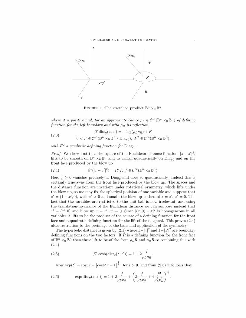
See Figure 1 in which (x, y) and (x′, y′) are local coordinates near a point in thecenter of the blow up, with boundary defining functions x and x′ in the two factors.

Thus Bn ×0 Bn has three boundary hypersurfaces, the front face introduced by

the blow up and the left and right boundary faces which map back to ∂Bn×Bn and

Bn × ∂Bn respectively under β. Denote by Diag0 the lift of the diagonal, which in

this case is the closure of the inverse image under β of the interior of the diagonalin B

n × Bn.

Lemma 2.1. Lifted to the interior of Bn ×0 Bn the hyperbolic distance function

extends smoothly up to the interior of the front face, in the complement of Diag0,


0

x’

x

y−y’

T

B

F

Diag

Diag

Figure 1. The stretched product Bn ×0 Bn.

where it is positive and, for an appropriate choice ρL ∈ C∞(Bn ×0 Bn) of defining

function for the left boundary and with ρR its reflection,

(2.3)β∗dist0(z, z

′) = − log(ρLρR) + F,

0 < F ∈ C∞(Bn ×0 Bn \Diag0), F

2 ∈ C∞(Bn ×0 Bn),

with F 2 a quadratic defining function for Diag0 .

Proof. We show first that the square of the Euclidean distance function, |z − z′|2,lifts to be smooth on B

n ×0 Bn and to vanish quadratically on Diag0 and on the

front face produced by the blow up

(2.4) β∗(|z − z′|2) = R2f, f ∈ C∞(Bn ×0 Bn).

Here f ≥ 0 vanishes precisely at Diag0 and does so quadratically. Indeed this iscertainly true away from the front face produced by the blow up. The spaces andthe distance function are invariant under rotational symmetry, which lifts underthe blow up, so me may fix the spherical position of one variable and suppose thatz′ = (1 − x′, 0), with x′ > 0 and small, the blow up is then of z = z′, x′ = 0. Thefact that the variables are restricted to the unit ball is now irrelevant, and usingthe translation-invariance of the Euclidean distance we can suppose instead thatz′ = (x′, 0) and blow up z = z′, x′ = 0. Since |(x, 0) − z|2 is homogeneous in allvariables it lifts to be the product of the square of a defining function for the frontface and a quadratic defining function for the lift of the diagonal. This proves (2.4)after restriction to the preimage of the balls and application of the symmetry.

The hyperbolic distance is given by (2.1) where 1−|z|2 and 1−|z′|2 are boundarydefining functions on the two factors. If R is a defining function for the front faceof Bn ×0 B

n then these lift to be of the form ρLR and ρRR so combining this with(2.4)

(2.5) β∗ cosh(dist0(z, z′)) = 1 + 2

f

ρLρR.

Now exp(t) = cosh t+[cosh2 t− 1

] 12 , for t > 0, and from (2.5) it follows that

(2.6) exp(dist0(z, z′)) = 1 + 2

f

ρLρR+

(2

f

ρLρR+ 4

f2

ρ2Lρ2R

) 12

.


Near Diag0 the square-root is dominated by the first part and near the left andright boundaries by the second part, and is otherwise positive and smooth. Takinglogarithms gives the result as claimed, with the defining function taken to be onenear Diag0 and to be everywhere smaller than a small positive multiple of (1 −|z|2)/R.

This result will be extended to the case of a perturbation of the hyperbolic met-ric by constructing the distance function directly from Hamilton-Jacobi theory, i.e.by integration of the Hamilton vector field of the metric function on the cotangentbundle. The presence of only simple logarithmic singularities in (2.3) shows, per-haps somewhat counter-intuitively, that the Lagrangian submanifold which is thegraph of the differential of the distance should be smooth (away from the diagonal)in the b-cotangent bundle of M2

0 . Conversely if this is shown for the perturbedmetric then the analogue of (2.3) follows except for the possibility of a logarithmicterm at the front face.

Since the metric is singular near the boundary, the dual metric function onT ∗

Bn is degenerate there. In terms of local coordinates near a boundary point, x,

y where the boundary is locally x = 0, and dual variables ξ, η, the metric functionfor hyperbolic space is of the form

(2.7) 2p0 = x2ξ2 + 4x2(1− x2)−2h0(ω, η)

where h0 is the metric function for the induced metric on the boundary.Recall that the 0-cotangent bundle of a manifold with boundary M, denoted

0T ∗M, is a smooth vector bundle overM which is a rescaled version of the ordinarycotangent bundle. In local coordinates near, but not at, the boundary these twobundles are identified by the (rescaling) map

(2.8) T ∗M ∋ (x, y, ξ, η) 7−→ (x, y, λ, µ) = (x, y, xξ, xη) ∈ 0T ∗M.

It is precisely this rescaling which makes the hyperbolic metric into a non-degeneratefiber metric, uniformly up to the boundary, on this bundle. On the other hand the b-cotangent bundle, also a completely natural vector bundle, is obtained by rescalingonly in the normal variable

(2.9) T ∗M ∋ (x, y, ξ, η) 7−→ (x, y, λ, η) = (x, y, xξ, η) ∈ bT ∗M.

Identification over the interior gives natural smooth vector bundle maps

(2.10) ιb0 : 0TM −→ bTM, ιtb0 : bT ∗M −→ 0T ∗M.

The second scaling map can be constructed directly in terms of blow up.

Lemma 2.2. If 0T ∗∂M ⊂ 0T ∗∂MM denotes the annihilator of the null space, over

the boundary, of ιb0 in (2.10) then there is a canonical diffeomorphism(2.11)

bT ∗M −→ [0T ∗M, 0T ∗∂M ] \ β#(0T ∗

∂MM), β : [0T ∗M, 0T ∗∂M ] −→ 0T ∗M,

to the complement, in the blow up, of the lift of the boundary:

β#(0T ∗∂MM) = β−1(0T ∗

∂MM \ 0T ∗∂M).

Proof. In local coordinates x, yj , the null space of ιb0 in (2.10) is precisely the spanof the ‘tangential’ basis elements x∂yj

over each boundary point. Its annihilator,0T ∗∂M is given in the coordinates (2.9) by µ = 0 at x = 0. The lift of the ‘oldboundary’ x = 0 is precisely the boundary hypersurface near which |µ| dominates


x. Thus, x is a valid defining function for the boundary of the complement, on theright in (2.11) and locally in this set, above the coordinate patch in M, ηj = µj/xare smooth functions. The natural bundle map bT ∗M −→ 0T ∗M underlying (2.11)

is given in these coordinates by λdxx + η · dy 7−→ λdx

x + xη · dyx , which is precisely

the same map, µ = xη, as appears in (2.9), so the result, including naturality,follows.

The symplectic form lifted to 0T ∗M is

0ω =1

xdλ ∧ dx+

1

xdµ ∧ dy −

1

x2dx ∧ (µ · dy)

whereas lifted to bT ∗M it is

(2.12) bω =1

xdλ ∧ dx+ dη ∧ dy.

Working, for simplicity of computation, in the non-compact upper half-spacemodel for hyperbolic space the metric function lifts to the non-degenerate quadraticform on 0T ∗M :

(2.13) 2p0 = λ2 + h0(ω, µ)

where h0 = |µ|2 is actually the Euclidean metric. The 0-Hamilton vector fieldof p0 ∈ C∞(0T ∗M), just the lift of the Hamilton vector field over the interior, isdetermined by

(2.14) 0ω(·, 0Hp) = dp.

Thus

0Hp = x

∂p

∂λ∂x + x

∂p

∂µ· ∂y −

(µ ·

∂p

∂µ+ x

∂p

∂x

)∂λ −

(−∂p

∂λµ+ x

∂p

∂y

)· ∂µ

and hence

(2.15) 0Hp0

= λ(x∂x + µ∂µ)− h0∂λ +x

2Hh0

is tangent to the smooth (up to the boundary) compact sphere bundle given byp0 = 1.

Over the interior of M = Bn, the hyperbolic distance from any interior point

of the ball is determined by the graph of its differential, which is the flow outinside p0 = 1, of the intersection of this smooth compact manifold with boundarywith the cotangent fiber to the initial point. Observe that Hp0

is also tangent tothe surface µ = 0 over the boundary, which is the invariantly defined subbundle0T ∗∂M. Since the coordinates can be chosen to be radial for any interior point, itfollows that all the geodesics from the interior arrive at the boundary at x = 0,µ = 0, corresponding to the well-known fact that hyperbolic geodesics are normal tothe boundary. This tangency implies that Hp0

lifts under the blow up of 0T ∗∂M in(2.11) to a smooth vector field on bTM ; this can also be seen by direct computation.

Lemma 2.3. The graph of the differential of the distance function from any interiorpoint, p ∈ (Bn), of hyperbolic space extends by continuity to a smooth Lagrangiansubmanifold of bT ∗(Bn \ p) which is transversal to the boundary, is a graph overBn \p and is given by integration of a non-vanishing vector field up to the bound-

ary.


Proof. Observe the effect of blowing up µ = 0, x = 0 on the Hamilton vector fieldin (2.15). As noted above, near the front face produced by this blow up validcoordinates are given by η = µ/x, λ and y, with x the boundary defining function.Since this transforms 0ω to bω it follows that 0

Hp0is transformed to

(2.16) bHp0

= x(λ∂x − xh0∂λ + xHh0)

where now Hh0is the Hamilton vector field with respect to y and η.

The constant energy surface p0 = 1 remains smooth, but non-compact, near theboundary, which it intersects transversally in λ = 1. From this the result follows– with the non-vanishing smooth vector field being b

Hp0divided by the boundary

defining function x near the boundary.

The logarithmic behaviour of the distance function in (2.3) with one point fixedin the interior is a consequence of Lemma 2.2, since the differential of the distancemust be of the form adx/x + b · dy for smooth functions a and b, and since it isclosed, a is necessarily constant on the boundary.

To examine the distance as a function of both variables a similar constructionfor the product, in this case M2, M = B

n can be used. The graph, Λ, of thedifferential of the distance d(p, p′) as a function on M2 is the joint flow out of theconormal sphere bundle to the diagonal in T ∗M2 = T ∗M × T ∗M, under the twoHamiltonian vector fields of the two metric functions within the product spherebundles. As before it is natural to lift to 0T ∗M × 0T ∗M where the two spherebundles extend smoothly up to the boundary. However, one can make a strongerstatement, namely that the lifted Hamilton vector fields are smooth on the b-cotangent bundle of M2

0 , and indeed even on the ‘partially b’-cotangent bundle ofM2

0 , with ‘partially’ meaning it is the standard cotangent bundle over the interiorof the front face. This is defined and discussed in more detail below; note that theidentification of these bundles over the interior of M2

0 extends to a smooth mapfrom these bundles to the lift of 0T ∗M × 0T ∗M , as we show later, explaining the‘stronger’ claim.

Smoothness of the Hamilton vector field together with transversality conditionsshows that the flow-out of the conormal bundle of the diagonal is a smooth La-grangian submanifold of the cotangent bundle under consideration; closeness to aparticular Lagrangian (such as that for hyperbolic space) restricted to which pro-jection to M2

0 is a diffeomorphism, guarantees that this Lagrangian is also a graphover M2

0 . Thus, over the interior, (M20 )

, it is the graph of the differential of thedistance function, and the latter is smooth; the same would hold globally if the La-grangian were smooth on T ∗M2

0 . The latter cannot happen, though the Lagrangianwill be a graph in the b-, and indeed the partial b-, cotangent bundles over M2

0 .These give regularity of the distance function, namely smoothness up to the frontface (directly for the partial b bundle, with a short argument if using the b bundle),and the logarithmic behavior up to the other faces. Note that had we only showedthe graph statement in the pullback of 0T ∗M × 0T ∗M, one would obtain directlyonly a weaker regularity statement for the distance function; roughly speaking, thecloser the bundle in which the Lagrangian is described is to the standard cotangentbundle, the more regularity the distance function has.

In fact it is possible to pass from the dual of the lifted product 0-tangent bundleto the dual of the b-tangent bundle, or indeed the partial b-bundle, by blow-up, as


for the single space above. Observe first that the natural inclusion

(2.17) ι0b × ι0b : 0TM × 0TM −→ bTM2 = bTM × bTM

identifies the sections of the bundle on the left with those sections of the bundleon the right, the tangent vector fields on M2, which are also tangent to the twofibrations, one for each boundary hypersurface

(2.18) φL : ∂M ×M −→M, φR :M × ∂M −→M.

Lemma 2.4. The fibrations (2.18), restricted to the interiors, extend by continuityto fibrations φL, resp. φR, of the two ‘old’ boundary hypersurfaces of M2

0 and thesmooth sections of the lift of 0TM × 0TM to M2

0 are naturally identified with thesubspace of the smooth sections of bTM2

0 which are tangent to these fibrations andalso to the fibres of the front face of the blow up, β0 : ff(M2

0 ) −→ ∂M × ∂M.

Proof. It is only necessary to examine the geometry and vector fields near the frontface produced by the the blow up of the diagonal near the boundary. Using thesymmetry between the two factors, it suffices to consider two types of coordinatesystems. The first is valid in the interior of the front fact and up to a general pointin the interior of the intersection with one of the old boundary faces. The secondis valid near a general point of the corner of the front face, which has fibers whichare quarter spheres.

For the first case let x, y and x′, y′ be the same local coordinates in two factors.The coordinates

(2.19) s = x/x′, x′, y and Y = (y′ − y)/x′

are valid locally in M20 above the point x = x′ = 0, y = y′, up to the lift of the old

boundary x = 0, which becomes locally s = 0. The fibration of this hypersurface isgiven by the constancy of y and the front face is x′ = 0 with fibration also givenby the constancy of y. The vector fields

x∂x, x∂y, x′∂x′ and x′∂y′

lift tos∂s, sx

′∂y − s∂Y , x′∂x′ − s∂s − Y · ∂Y and ∂Y .

The basis s∂s, sx′∂y, x

′∂x′ and ∂Y shows that these vector fields are locally preciselythe tangent vector fields also tangent to both fibrations.

After relabeling the tangential variables as necessary, and possibly switchingtheir signs, so that y′1 − y1 > 0 is a dominant variable, the coordinate system

(2.20) t = y′1 − y1, s1 =x

y′1 − y1, s2 =

x′

y′1 − y1, Zj =

y′j − yj

y′1 − y1, j > 1, y

can be used at a point in the corner of the front face. The three boundary hyper-surfaces are locally s1 = 0, s2 = 0 and t = 0 and their respective fibrations aregiven in these coordinates by

(2.21)

s1 = 0, y = const.,

s2 = 0, y′1 = y1 + t = const., y′j = yj + tZj = const., j > 1,

t = 0, y = const.

Thus, the intersections of fibres of the lifted left or right faces with the front faceare precisely boundary hypersurfaces of fibres there. On the other hand within theintersection of the lifted left and right faces the respective fibres are transversal


except at the boundary representing the front face. The lifts of the basis of thezero vector fields is easily computed:

(2.22)

x∂x 7−→ s1∂s1 ,

x∂y1−→ −s1t∂t + s21∂s1 + s1s2∂s2 + s1Z · ∂Z + s1t∂y1

,

x∂yj7−→ s1t∂yj

− s1∂Zj,

x′∂x′ 7−→ s2∂s2 ,

x′∂y′1−→ s2t∂t − s2s1∂s1 − s22∂s2 − s2Z · ∂Z ,

x′∂y′j7−→ s2∂Zj

.

The span, over C∞(M20 ), of these vector fields is also spanned by

s1∂s1 , s2∂s2 , s2∂Zj, j > 1, s1(t∂yj

−∂Zj), j > 1, s1(t∂t− t∂y1

−Z ·∂Z) and s2t∂t.

These can be seen to locally span the vector fields tangent to all three boundariesand corresponding fibrations, proving the Lemma.

With φ = φL, φR, β0 the collection of boundary fibrations, we denote by φTM20

the bundle whose smooth sections are exactly the smooth vector fields tangent toall boundary fibrations. Thus, the content of the preceding lemma is that

β∗(0TM × 0TM) = φTM20 .

These fibrations allow the reconstruction of bT ∗M20 as a blow up of the lift of

0T ∗M× 0T ∗M toM20 . It is also useful, for more precise results later on, to consider

the ‘partially b-’ cotangent bundle of M20 ,

b,ffT ∗M20 ; this is the dual space of the

partially b-tangent bundle, b,ffTM20 , whose smooth sections are smooth vector fields

on M20 which are tangent to the old boundaries, but not necessarily to the front

face, ff. Thus, in coordinates (2.19), s∂s, ∂x′ , ∂y and ∂Y form a basis of b,ffTM20 ,

while in coordinates (2.20), s1∂s1 , s2∂s2 , ∂t, ∂Zjand ∂y do so. Let

ι20b : φTM20 → bTM2

0 , ι20b,ff : φTM2

0 → b,ffTM20

be the inclusion maps.

Lemma 2.5. The annihilators, in the lift of 0T ∗M×0T ∗M toM20 , of the null space

of either ι20b or ι20b,ff over the old boundaries, as in Lemma 2.4, form transversalembedded p-submanifolds. After these are blown up, the closure of the annihilatorof the nullspace of ι20b, resp. ι20b,ff , over the interior of the front face of M2

0 is ap-submanifold, the subsequent blow up of which produces a manifold with cornerswith three ‘old’ boundary hypersurfaces; the complement of these three hypersurfacesis canonically diffeomorphic to bT ∗M2

0 , resp.b,ffT ∗M2

0 .

Proof. By virtue of Lemma 2.2 and the product structure away from the front face ffofM2

0 , the statements here are trivially valid except possibly near ff. We may againuse the coordinate systems discussed in the proof of Lemma 2.4. Consider the linearvariables in the fibres in which a general point is lx∂x + v · x∂y + l′x′∂x′ + v′ · x′∂y′ .

First consider the inclusion into bTM20 . In the interiors of s1 = 0 and s2 = 0

and the front face respectively, the null bundles of the inclusion into the tangent


vector fields are(2.23)

l = l′ = 0, v′ = 0,

l = l′ = 0, v = 0,

ls∂s + v(sx′∂y − s∂Y ) + l′(x′∂x′ − s∂s − Y ∂Y ) + v′∂Y = 0 at x′ = 0, s > 0

⇐⇒ l = l′ = 0, v′ = sv.

The corresponding annihilator bundles, over the interiors of the boundary hy-persurfaces of M2

0 , in the dual bundle, with basis

(2.24) λdx

x+ µ

dy

x+ λ′

dx′

x′+ µ′ dy

′

x′

are therefore, as submanifolds,

(2.25)

s1 = 0, µ = 0,

s2 = 0, µ′ = 0 and

x′ = 0, µ+ sµ′ = 0 or t = 0, s2µ+ s1µ′ = 0.

Here the annihilator bundle over the front face is given with respect to both thecoordinate system (2.19) and (2.20).

Thus, the two subbundles over the old boundary hypersurfaces meet transversallyover the intersection, up to the corner, as claimed and so can be blown up in eitherorder. In the complement of the lifts of the old boundaries under these two blow ups,the variables µ/s1 and µ′/s2 become legitimate; in terms of these the subbundleover the front face becomes smooth up to, and with a product decomposition at,all its boundaries. Thus, it too can be blown up. That the result is a (painful)reconstruction of the b-cotangent bundle of the blown up manifold M2

0 followsdirectly from the construction.

It remains to consider the inclusion into b,ffTM20 . The only changes are at the

front face, namely the third line of (2.23) becomes(2.26)

ls∂s + v(sx′∂y − s∂Y ) + l′(x′∂x′ − s∂s − Y ∂Y ) + v′∂Y = 0 at x′ = 0, s > 0

⇐⇒ l = l′, v′ = sv + l′Y.

Correspondingly the third line of (2.25) becomes

(2.27)

x′ = 0, λ+ λ′ + µ′Y = 0, µ+ sµ′ = 0

or t = 0, s2µ+ s1µ′ = 0, s2(λ+ λ′) + µ′

1 +∑

j≥2

µ′jZj = 0.

The rest of the argument is unchanged, except that the conclusion is that b,ffT ∗M20

is being reconstructed.

Note that for any manifold with corners, X, the b-cotangent bundle of anyboundary hypersurface H (or indeed any boundary face) includes naturally as asubbundle bT ∗H → bT ∗

HX.

Lemma 2.6. The Hamilton vector field of gδ lifts from either the left or the rightfactor of M in M2 to a smooth vector field, tangent to the boundary hypersurfaces,on bT ∗M2

0 , as well as on b,ffT ∗M20 , still denoted by H

Lgδ, resp. H

Rgδ. Moreover,

HLgδ

= ρLVL, HR

gδ= ρRV

R, where VL, resp. VR are smooth vector fields tangent to


all hypersurfaces except the respective cotangent bundles over the left, resp. right,boundaries, to which they are transversal, and where ρL and ρR are defining func-tions of the respective cotangent bundles over these boundaries.

Proof. Inserting the explicit form of the Euclidean metric, the Hamilton vector fieldin (2.15) becomes

(2.28) 0Hp0

= λ(x∂x + µ∂µ)− |µ|2∂λ + xµ · ∂y.

Consider the lift of this vector field to the product, 0T ∗M × 0T ∗M, from left andright, and then under the blow up of the diagonal in the boundary. In the coordinatesystems (2.19) and (2.20)

(2.29)

0H

Lp0

= λ(s∂s + µ∂µ)− |µ|2∂λ + sµ(x′∂y − ∂Y )

0H

Rp0

= λ′(x′∂x′ − s∂s − Y ∂Y + µ′∂µ′)− |µ′|2∂λ′ + µ′∂Y

0H

Lp0

= λ(s1∂s1 + µ∂µ)− |µ|2∂λ + s1∑

j≥2

µj(t∂yj− ∂Zj

)

+s1µ1(t∂y1− t∂t + s1∂s1 + s2∂s2 +

∑

j≥2

Zj∂Zj)

0H

Rp0

= λ′(s2∂s2 + µ′∂µ′)− |µ′|2∂λ′ + s2∑

j≥2

µ′j∂Zj

+s2µ′1(t∂t − s1∂s1 − s2∂s2 −

∑

j≥2

Zj∂Zj).

Note that the bundle itself is just pulled back here, so only the base variables arechanged.

Next we carry out the blow ups of Lemma 2.5. The centers of blow up are givenexplicitly, in local coordinates, in (2.25), with the third line replaced by (2.27) inthe case of ι20b,ff . We are only interested in the behaviour of the lifts of the vector

fields in (2.29) near the front faces introduced in the blow ups.Consider ι20b first. For the first two cases there are two blow-ups, first of µ = 0

in s = 0 and then of µ + sµ′ = 0 in x′ = 0. Thus, near the front face of the firstblow up, the µ variables are replaced by µ = µ/s and then the center of the secondblow up is µ + µ′ = 0, x′ = 0. Thus, near the front face of the second blow up wecan use as coordinates s, x′, µ′ and ν = (µ+ µ′)/x′, i.e. substitute µ = −µ′ + x′ν.In the coordinate patch (2.29) the lifts under the first blow up are

(2.30)

0H

Lp0

7−→ λs∂s − s2|µ|2∂λ + s2µ(x′∂y − ∂Y )

0H

Rp0

7−→ λ′(x′∂x′ − s∂s − Y ∂Y + µ∂µ + µ′∂µ′)− |µ′|2∂λ′ + µ′∂Y .

Thus under the second blow up, the left Hamilton vector field lifts to

(2.31) 0H

Lp0

7−→ sT, T = λ∂s − s|µ|2∂λ + sµ(x′∂y − ∂Y )

where T is transversal to the boundary s = 0 where λ 6= 0.A similar computation near the corner shows the lifts of the two Hamilton vector

fields under blow up the fibrations of s1 = 0 and s2 = 0 in terms of the new


coordinates µ = µ/s1 and µ′ = µ′/s2 to be

(2.32)

0H

Lp0

=λs1∂s1 − s21|µ|2∂λ + s21

∑

j≥2

µj(t∂yj− ∂Zj

)

+s21µ1(t∂y1− t∂t + s1∂s1 − µ∂µ + s2∂s2 − µ′∂µ′ +

∑

j≥2

Zj∂Zj),

0H

Rp0

=λ′s2∂s2 − s22|µ′|2∂λ′ + s22

∑

j≥2

µ′j∂Zj

+s22µ′1(t∂t − s1∂s1 + µ∂µ − s2∂s2 + µ′∂µ′ −

∑

j≥2

Zj∂Zj).

The final blow up is that of t = 0, µ + µ′ = 0, near the front face of this blow-upreplacing (t, µ, µ′) by (t, µ, ν), ν = (µ + µ′)/t, as valid coordinates (leaving theothers unaffected). Then the vector fields above become

(2.33)

0H

Lp0

= s1TL, 0

HRp0

= s2TR,

TL =λ∂s1 − s1|µ|2∂λ + s1

∑

j≥2

µj(t∂yj− ∂Zj

)

+s1µ1(t∂y1− t∂t + s1∂s1 − µ∂µ + s2∂s2 +

∑

j≥2

Zj∂Zj),

TR =λ′∂s2 − s2|µ′|2∂λ′ + s2

∑

j≥2

µ′j∂Zj

+s2µ′1(t∂t − s1∂s1 + µ∂µ − s2∂s2 −

∑

j≥2

Zj∂Zj).

Thus both left and right Hamilton vector fields are transversal to the respectiveboundaries after a vanishing factor is removed, provided λ, λ′ 6= 0.

The final step is to show that the same arguments apply to the perturbed metric.First consider the lift, from left and right, of the perturbation to the Hamilton vectorfield arising from the perturbation of the metric. By assumption, the perturbationH is a 2-cotensor which is smooth up to the boundary. Thus, as a perturbationof the dual metric function on 0T ∗M it vanishes quadratically at the boundary.In local coordinates near a boundary point it follows that the perturbation of thedifferential of the metric function is of the form

(2.34) dp− dp0 = x2(adx

x+ bdy + cdλ+ edµ)

From (2.14) it follows that the perturbation of the Hamilton vector field is of theform

(2.35) Hp − Hp0= x2(a′x∂x + b′x∂y + c′∂λ + e′∂µ)

on 0T ∗M. Lifted from the right or left factors to the product and then under theblow-up of the diagonal to M2

0 it follows that in the coordinate systems (2.19) and(2.20), the perturbations are of the form

(2.36)H

Lp − H

Lp0

= s2(x′)2V L, HRp − H

Rp0

= (x′)2V R, V L, V R ∈ Vb,

HLp − H

Lp0

= s21t2WL, HR

p − HRp0

= s22t2WR, WR, WR ∈ Vb

where Vb denotes the space of smooth vector fields tangent to all boundaries. Sincethe are lifted from the right and left factors, V L and V R are necessarily tangent


to the annihilator submanifolds of the right and left boundaries. It follows thatthe vector fields sx′V L and x′V R are tangent to both fibrations above a coordi-nate patch as in (2.19) and s1tV

L and s2tVR are tangent to all three annihilator

submanifolds above a coordinate patch (2.20). Thus, after the blow ups whichreconstruct bT ∗M2

0 , the perturbations lift to be of the form

(2.37) HLp − H

Lp0

= ρLρffUL, HR

p − HRp0

= ρRρffUR

where UL and UR are smooth vector fields on bT ∗M20 .

From (2.37) it follows that the transversality properties in (2.31) and (2.33)persist.

Now consider ι20b,ff . First, (2.30) is unchanged, since the annihilators on the ‘old’

boundary faces are the same in this case. In particular, we still have µ = µ/s as oneof our coordinates after the first blow up; the center of the second blow up is thenx′ = 0, λ+λ′ +µ′ ·Y = 0, µ+µ′ = 0. Thus, near the front face of the second blowup we can use as coordinates s, x′, µ′ and σ = (λ+λ′ +µ′ ·Y )/x′, ν = (µ+µ′)/x′,i.e. substitute µ = −µ′ + x′ν, i.e. µ = −µ′s + x′sν, and λ = −λ′ − µ′ · Y + x′σ.Thus under the second blow up, the left Hamilton vector field lifts to

(2.38) 0H

Lp0

7−→ sT ′, T ′ = λ∂s + µ · (−ν∂σ + x′∂y − ∂Y ),

so T ′ is transversal to the boundary s = 0 where λ 6= 0.In the other coordinate chart, again, (2.32) is unchanged since the annihilators

on the ‘old’ boundary faces are the same. The final blow up is that of

t = 0, µ+ µ′ = 0, λ+ λ′ + µ′1 +

∑

j≥2

µ′jZj = 0,

near the front face of this blow-up replacing (t, µ, µ′, λ, λ′) by (t, µ, ν, λ, σ),

ν = (µ+ µ′)/t, σ = (λ+ λ′ + µ′1 +

∑

j≥2

µ′jZj)/t,

as valid coordinates (leaving the others unaffected). Then the vector fields abovebecome

(2.39)

0H

Lp0

= s1TL, 0

HRp0

= s2TR,

TL =λ∂s1 − s1|µ|2∂λ + s1

∑

j≥2

µj(t∂yj− ∂Zj

− νj∂σ)

+s1µ1(t∂y1− t∂t + s1∂s1 + σ∂σ − ν∂ν + s2∂s2 − ν1∂σ +

∑

j≥2

Zj∂Zj),

TR =λ′∂s2 + s2∑

j≥2

µ′j∂Zj

+s2µ′1(t∂t − s1∂s1 + µ∂µ − s2∂s2 − σ∂σ −

∑

j≥2

Zj∂Zj).

Again, both left and right Hamilton vector fields are transversal to the respectiveboundaries after a vanishing factor is removed, provided λ, λ′ 6= 0. The rest of theargument proceeds as above.

Proposition 2.7. The differential of the distance function for the perturbed metricgδ, for sufficiently small δ, on M = B

n defines a global smooth Lagrangian subman-ifold Λδ, of

bT ∗(M ×0M), which is a smooth section outside the lifted diagonal andwhich lies in bT ∗ ff over the front face, ff(M2

0 ) and in consequence there is a unique


geodesic between any two points of (B3), no conjugate points and (2.3) remainsvalid for distδ(z, z

′).

Proof. For the unperturbed metric this already follows from Lemma 2.1. We firstreprove this result by integrating the Hamilton vector fields and then examine theeffect of the metric perturbation. Thus we first consider the lift of the Hamiltonvector field of the hyperbolic distance function from 0T ∗M, from either the left ofthe right, to b,ffT ∗M2

0 , using the preceding lemma.Although the global regularity of the Lagrangian which is the graph of the dif-

ferential of the distance is already known from the explicit formula in this case,note that it also follows from the form of these two vector fields. The initial mani-fold, the unit conormal bundle to the diagonal, becomes near the corner of M2 thevariety of those

(2.40) ξ(dx− dx′) + η(dy − dy′) such that ξ2 + |η|2 =1

2x2, x = x′ > 0, y = y′.

In the blown up manifold M20 the closure is smooth in bT ∗M2

0 and is the bundleover the lifted diagonal given in terms of local coordinates (2.19) by

(2.41) λds

s+ µdY, λ2 + |µ|2 =

1

2, s = 1, Y = 0;

the analogous statement also holds in b,ffT ∗M20 where one has the ‘same’ expression.

Using the Hamilton flow in b,ffT ∗M20 , we deduce that the flow out is a global smooth

submanifold, where smoothness includes up to all boundaries, of b,ffT ∗M20 , and is

also globally a graph away from the lifted diagonal, as follows from the explicitform of the vector fields. Note that over the interior of the front face, b,ffT ∗M2

0 isjust the standard cotangent bundle, so smoothness of the distance up to the frontface follows. Over the left and right boundaries the Lagrangian lies in λ = 1 andλ′ = 1 so the form (2.3) of the distance follows.

The analogous conclusion can also be obtained by using the flow in bT ∗M20 . In

this setting, we need that over the front face (2.41) is contained in the image ofbT ∗ ff to which both lifted vector fields are tangent. Thus it follows that the flow outis a global smooth submanifold, where smoothness includes up to all boundaries, ofbT ∗M2

0 which is contained in the image of bT ∗ ff over ff(M20 ). Again, it is globally a

graph away from the lifted diagonal, as follows from the explicit form of the vectorfields. Over the left and right boundaries the Lagrangian lies in λ = 1 and λ′ = 1so the form (2.3) of the distance follows.

For small δ these perturbation of the Hamilton vector fields are also small insupremum norm and have the same tangency properties at the boundaries usedabove to rederive (2.3), from which the Proposition follows.

3. The semiclassical double space

In this section we construct the semiclassical double space, M0,~, which will bethe locus of our parametrix construction. To motivate the construction, we recallthat Mazzeo and the first author [16] have analyzed the resolvent R(h, σ), defined inequation (17), for σ/h ∈ C, though the construction is not uniform as |σ/h| → ∞.They achieved this by constructing the Schwartz kernel of the parametrix G(h, σ)to R(h, σ) as a conormal distribution defined on the manifold

M0 = Bn+1 ×0 B

n+1


defined in (2.2), see also figure 1, with meromorphic dependence on σ/h.The manifold B

n+1 × Bn+1 is a 2n + 2 dimensional manifold with corners. It

contains two boundary components of codimension one, denoted as in [16] by

∂l1(Bn+1 × B

n+1) = ∂Bn+1 × Bn+1 and ∂r1(B

n+1 × Bn+1) = B

n+1 × ∂Bn+1,

which have a common boundary ∂2(Bn+1 × B

n+1) = ∂Bn+1 × ∂Bn+1. The lift of∂r1(B

n+1 × Bn+1) to M0, which is the closure of

β−1(∂r1(Bn+1 × B

n+1) \ ∂2(Bn+1 × B

n+1)),

with β : M0 → Bn+1 × B

n+1 the blow-down map, will be called the right face anddenoted by R. Similarly, the lift of ∂l1(B

n+1 ×Bn+1) will be called the left face and

denoted by L. The lift of Diag∩∂2(Bn+1 × B

n+1), which is its inverse image underβ, will be called the front face F , see figure 1.

We briefly recall the definitions of their classes of pseudodifferential operators,and refer the reader to [16] for full details. First they define the class Ψm

0 (Bn+1)which consists of those pseudodifferential operators of order m whose Schwartzkernels lift under the blow-down map β defined in (2.2) to a distribution whichis conormal (of order m) to the lifted diagonal and vanish to infinite order at allfaces, with the exception of the front face, up to which it is C∞ (with values inconormal distributions). Here, and elsewhere in the paper, we trivialized the rightdensity bundle using a zero-density; we conveniently fix this as |dgδ(z

′)|. Thus,the Schwartz kernel of A ∈ Ψm

0 (Bn+1) is KA(z, z′)|dgδ(z

′)|, with KA as describedabove, so in particular is C∞ up to the front face.

It then becomes necessary to introduce another class of operators whose kernels

are singular at the right and left faces. This class will be denoted by Ψm,a,b0 (Bn+1),

a, b ∈ C. An operator P ∈ Ψm,a,b0 (Bn+1) if it can be written as a sum P = P1 +P2,

where P1 ∈ Ψm0 (X) and the Schwartz kernel KP2

|dgδ(z′)| of the operator P2 is such

that KP2lifts under β to a conormal distribution which is smooth up to the front

face, and which satisfies the following conormal regularity with respect to the otherfaces

(3.1) Vkb β

∗KP2∈ ρaLρ

bRL

∞(Bn+1 ×0 Bn+1), ∀ k ∈ N,

where Vb denotes the space of vector fields on M0 which are tangent to the rightand left faces.

Next we define the semiclassical blow-up of

Bn+1 × B

n+1 × [0, 1)h,

and the corresponding classes of pseudodifferential operators associated with itthat will be used in the construction of the parametrix. The semiclassical doublespace is constructed in two steps. First, as in [16], we blow-up the intersectionof the diagonal Diag×[0, 1) with ∂Bn+1 × ∂Bn+1 × [0, 1). Then we blow-up theintersection of the lifted diagonal times [0, 1) with h = 0. We define the manifoldwith corners

(3.2) M0,~ = [Bn+1 × Bn+1 × [0, 1]h; ∂Diag×[0, 1);Diag0 ×0].

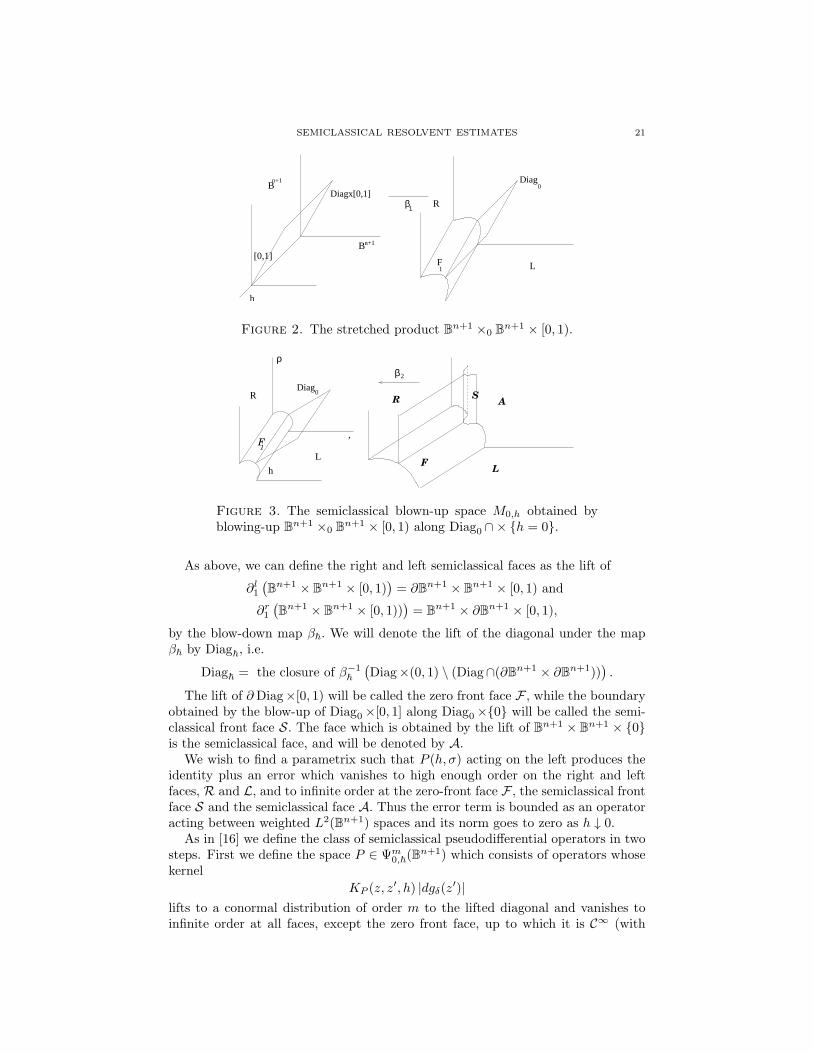
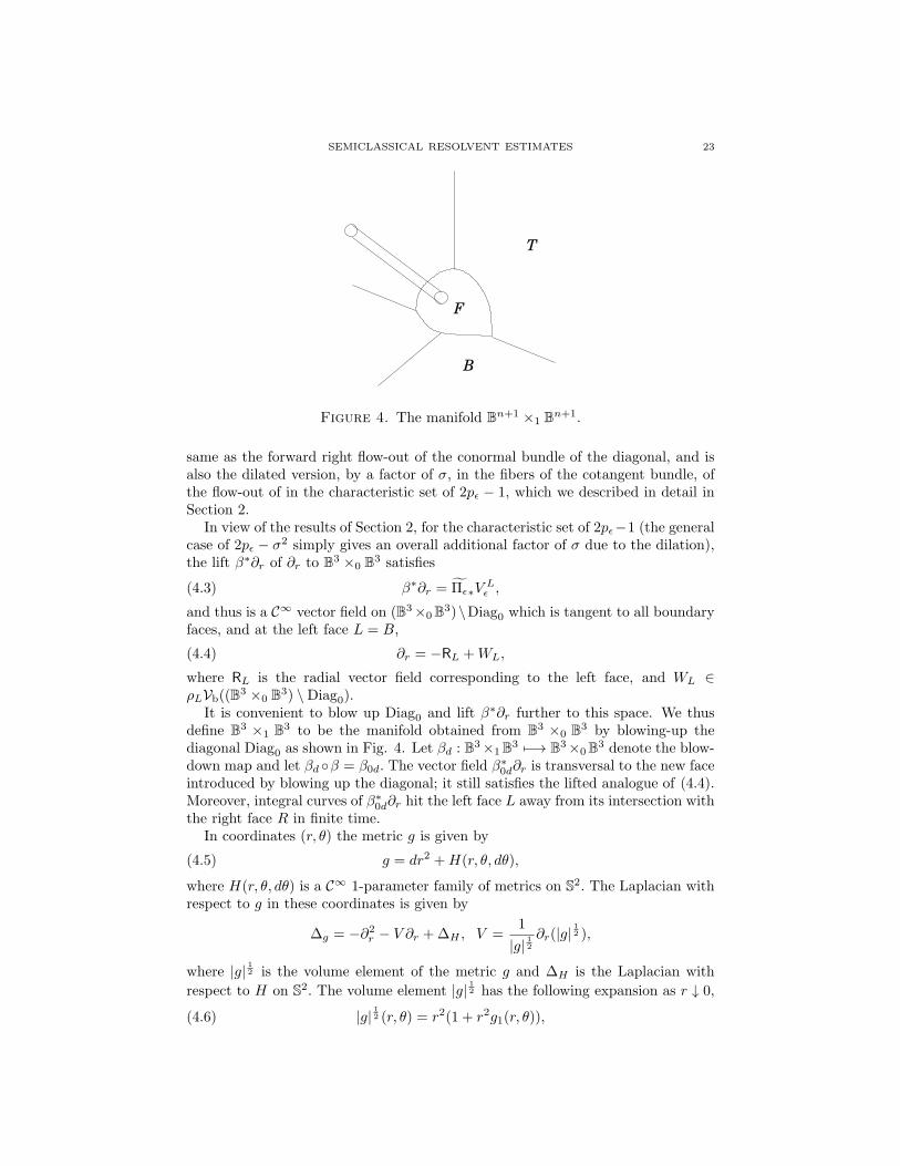
See Figures 2 and 3. We will denote the blow-down map

(3.3) β~ :M0,~ −→ Bn+1 × B

n+1 × [0, 1).


R

Bn+1

Diagx[0,1]

[0,1]

β1

h

F1

Diag0B

n+1

L

Figure 2. The stretched product Bn+1 ×0 Bn+1 × [0, 1).

S

β2

’

ρ

h

Diag

F1

L

R0

L

R

F

A

Figure 3. The semiclassical blown-up space M0,h obtained byblowing-up B

n+1 ×0 Bn+1 × [0, 1) along Diag0 ∩ × h = 0.

As above, we can define the right and left semiclassical faces as the lift of

∂l1(Bn+1 × B

n+1 × [0, 1))= ∂Bn+1 × B

n+1 × [0, 1) and

∂r1(Bn+1 × B

n+1 × [0, 1)))= B

n+1 × ∂Bn+1 × [0, 1),

by the blow-down map β~. We will denote the lift of the diagonal under the mapβ~ by Diag~, i.e.

Diag~ = the closure of β−1~

(Diag×(0, 1) \ (Diag∩(∂Bn+1 × ∂Bn+1))

).

The lift of ∂Diag×[0, 1) will be called the zero front face F , while the boundaryobtained by the blow-up of Diag0 ×[0, 1] along Diag0 ×0 will be called the semi-classical front face S. The face which is obtained by the lift of Bn+1 × B

n+1 × 0is the semiclassical face, and will be denoted by A.

We wish to find a parametrix such that P (h, σ) acting on the left produces theidentity plus an error which vanishes to high enough order on the right and leftfaces, R and L, and to infinite order at the zero-front face F , the semiclassical frontface S and the semiclassical face A. Thus the error term is bounded as an operatoracting between weighted L2(Bn+1) spaces and its norm goes to zero as h ↓ 0.

As in [16] we define the class of semiclassical pseudodifferential operators in twosteps. First we define the space P ∈ Ψm

0,~(Bn+1) which consists of operators whose

kernel

KP (z, z′, h) |dgδ(z

′)|

lifts to a conormal distribution of order m to the lifted diagonal and vanishes toinfinite order at all faces, except the zero front face, up to which it is C∞ (with


values in conormal distributions) and the semiclassical front face, up to which it ish−n−1C∞ (with values in conormal distributions). We then define the space

Ka,b,c(M0,~) = K ∈ L∞(M0,~) : Vmb K ∈ ρaLρ

bAρ

cRρ

−n−1S L∞(M0,~), m ∈ N,

(3.4)

where Vb denotes the Lie algebra of vector fields which are tangent to L, A and

R. Again, as in [16], we define the space Ψm,a,b,c0,~ (Bn+1) as the operators P which

can be expressed in the form P = P1 + P2, with P1 ∈ Ψm0,~(B

n+1) and the kernel

KP2|dgδ(z

′)| of P2 is such β∗~KP2

∈ Ka,b,c(M0,~).

4. A semiclassical parametrix for the resolvent in dimension three

In this section we construct a parametrix for the resolvent R(h, σ) defined in(17) in dimension three. We do this case separately because it is much simplerthan in the general case, and one does not have to perform the semiclassical blow-up. Besides, we will also need part of this construction in the general case. Moreprecisely, if n + 1 = 3, and the metric g satisfies the hypotheses of Proposition2.7, we will use Hadamard’s method to construct the leading asymptotic term ofthe parametrix G(σ, h) at the diagonal, and the top two terms of the semiclassicalasymptotics. Our construction takes place on (B3 ×0 B

3) × [0, 1)h, instead of itssemiclassical blow up, i.e. the blow up of the zero-diagonal at h = 0, as describedabove. This is made possible by a coincidence, namely that in three dimensions,apart from an explicit exponential factor, the leading term in the asymptotics liveson B

3 ×0 B3 × [0, 1). However, to obtain further terms in the asymptotics would

require the semiclassical blow up, as it will be working in higher dimensions. Forexample, this method only give bounds for the resolvent of width 1, while the moregeneral construction gives the bounds on any strip.

We recall that in three dimensions the resolvent of the Laplacian in hyperbolicspace, ∆g0 , R0(σ) = (∆g0 − σ2 − 1)−1 has a holomorphic continuation to C as anoperator from functions vanishing to infinite order at ∂B3 to distributions in B

3.The Schwartz kernel of R0(σ) is given by

R0(σ, z, z′) =

e−iσr0

4π sinh r0,(4.1)

where r0 = r0(z, z′) is the geodesic distance between z and z′ with respect to the

metric g0, see for example [16].Since there are no conjugate points for the geodesic flow of g, for each z′ ∈

(B3), the exponential map for the metric g, expg : Tz′(B3) −→ (B3), is a globaldiffeomorphism. Let (r, θ) be geodesic normal coordinates for g which are validin (B3) \ z′; r(z, z′) =: d(z, z′) is the distance function for the metric g. Sincer(z, z′) is globally defined, g is a small perturbation of g0 and the kernel of R0(σ)is given by (4.1), it is reasonable to seek a parametrix of R(h, σ) which has kernelof the form

G(h, σ, z, z′) = e−iσhrh−2U(h, σ, z, z′),(4.2)

with U properly chosen.We now reinterpret this as a semiclassical Lagrangian distribution to relate it to

the results of Section 2. Thus, −σr = −σd(z, z′) is the phase function for semi-classical distributions corresponding to the backward left flow-out of the conormalbundle of the diagonal inside the characteristic set of 2pǫ − σ2. This flowout is the


F

B

T

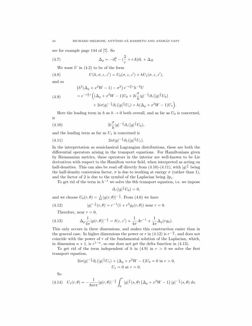
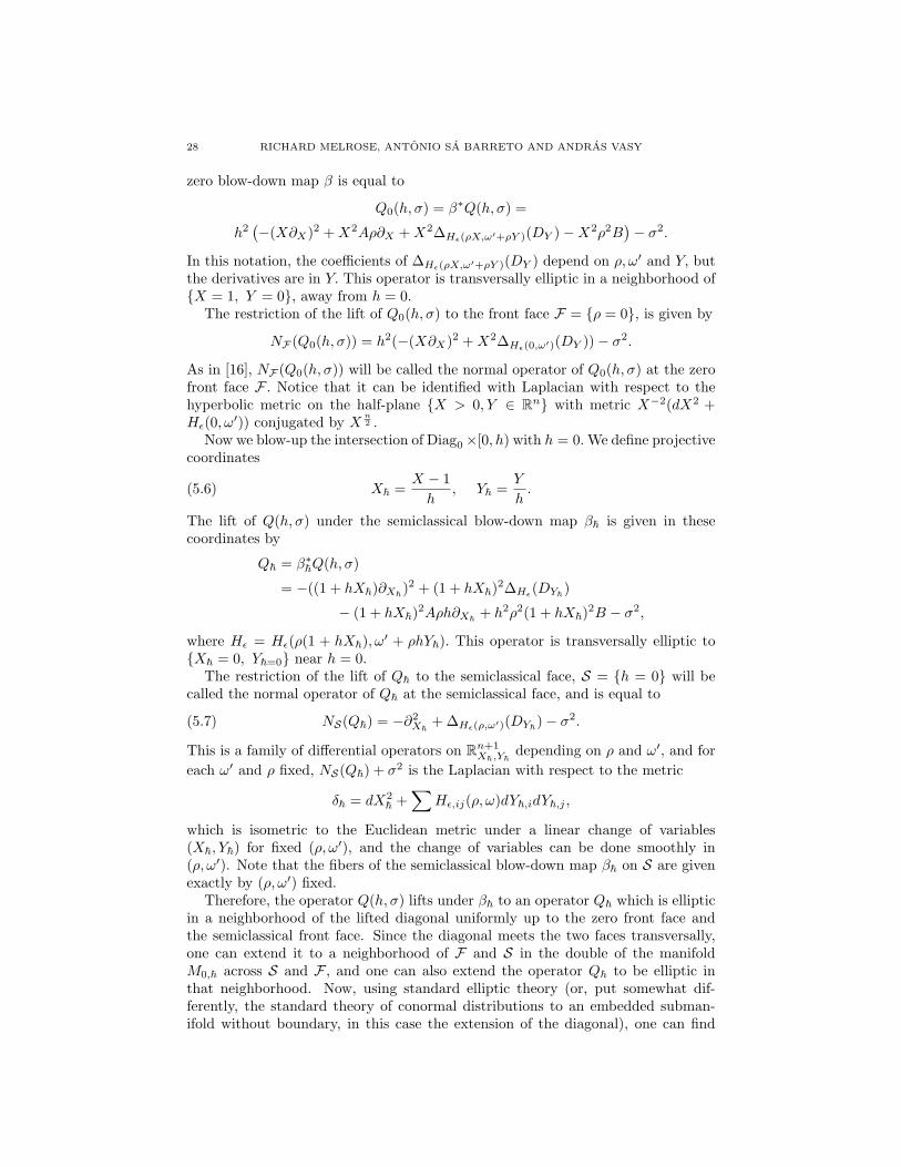
Figure 4. The manifold Bn+1 ×1 B

n+1.

same as the forward right flow-out of the conormal bundle of the diagonal, and isalso the dilated version, by a factor of σ, in the fibers of the cotangent bundle, ofthe flow-out of in the characteristic set of 2pǫ − 1, which we described in detail inSection 2.

In view of the results of Section 2, for the characteristic set of 2pǫ−1 (the generalcase of 2pǫ − σ2 simply gives an overall additional factor of σ due to the dilation),the lift β∗∂r of ∂r to B

3 ×0 B3 satisfies

(4.3) β∗∂r = Πǫ∗VLǫ ,

and thus is a C∞ vector field on (B3×0B3)\Diag0 which is tangent to all boundary

faces, and at the left face L = B,

(4.4) ∂r = −RL +WL,

where RL is the radial vector field corresponding to the left face, and WL ∈ρLVb((B

3 ×0 B3) \Diag0).

It is convenient to blow up Diag0 and lift β∗∂r further to this space. We thusdefine B

3 ×1 B3 to be the manifold obtained from B

3 ×0 B3 by blowing-up the

diagonal Diag0 as shown in Fig. 4. Let βd : B3×1B3 7−→ B

3×0B3 denote the blow-

down map and let βd β = β0d. The vector field β∗0d∂r is transversal to the new face

introduced by blowing up the diagonal; it still satisfies the lifted analogue of (4.4).Moreover, integral curves of β∗

0d∂r hit the left face L away from its intersection withthe right face R in finite time.

In coordinates (r, θ) the metric g is given by

g = dr2 +H(r, θ, dθ),(4.5)

where H(r, θ, dθ) is a C∞ 1-parameter family of metrics on S2. The Laplacian with

respect to g in these coordinates is given by

∆g = −∂2r − V ∂r +∆H , V =1

|g|12

∂r(|g|12 ),

where |g|12 is the volume element of the metric g and ∆H is the Laplacian with

respect to H on S2. The volume element |g|

12 has the following expansion as r ↓ 0,

|g|12 (r, θ) = r2(1 + r2g1(r, θ)),(4.6)


see for example page 144 of [7]. So

∆g = −∂2r − (2

r+ rA)∂r +∆H(4.7)

We want U in (4.2) to be of the form

U(h, σ, z, z′) = U0(σ, z, z′) + hU1(σ, z, z

′),(4.8)

and so (h2(∆g + x2W − 1)− σ2

)e−iσ

hrh−2U

= e−iσhr((∆g + x2W − 1)U0 + 2i

σ

h|g|−

14 ∂r(|g|

14U0)

+ 2iσ|g|−14 ∂r(|g|

14U1) + h(∆g + x2W − 1)U1

).

(4.9)

Here the leading term in h as h→ 0 both overall, and as far as U0 is concerned,is

(4.10) 2iσ

h|g|−

14 ∂r(|g|

14U0),

and the leading term as far as U1 is concerned is

(4.11) 2iσ|g|−14 ∂r(|g|

14U1).

In the interpretation as semiclassical Lagrangian distributions, these are both thedifferential operators arising in the transport equations. For Hamiltonians givenby Riemannian metrics, these operators in the interior are well-known to be Liederivatives with respect to the Hamilton vector field, when interpreted as acting onhalf-densities. This can also be read off directly from (4.10)-(4.11), with |g|

14 being

the half-density conversion factor, σ is due to working at energy σ (rather than 1),and the factor of 2 is due to the symbol of the Laplacian being 2pǫ.

To get rid of the term in h−1 we solve the 0th transport equation, i.e. we impose

∂r(|g|14U0) = 0,

and we choose U0(r, θ) =14π |g(r, θ)|

− 14 . From (4.6) we have

|g|−14 (r, θ) = r−1(1 + r2g2(r, θ)) near r = 0.(4.12)

Therefore, near r = 0,

∆g1

4π|g(r, θ)|−

14 = δ(z, z′) +

1

4πAr−1 +

1

4π∆g(rg2).(4.13)

This only occurs in three dimensions, and makes this construction easier than inthe general case. In higher dimensions the power or r in (4.12) is r−

n2 , and does not

coincide with the power of r of the fundamental solution of the Laplacian, which,in dimension n+ 1, is r1−n, so one does not get the delta function in (4.13).

To get rid of the term independent of h in (4.9) in r > 0 we solve the firsttransport equation,

2iσ|g|−14 ∂r(|g|

14U1) + (∆g + x2W − 1)U0 = 0 in r > 0,

U1 = 0 at r = 0.

So

U1(r, θ) = −1

8iσπ|g(r, θ)|−

14

∫ r

0

|g|14 (s, θ)

(∆g + x2W − 1

)|g|−

14 (s, θ) ds.(4.14)


Since |g|14 is C∞ up to r = 0, and vanishes at r = 0, it follows from (4.13) that

|g|14∆g|g|

− 14 is C∞ up to r = 0. In particular the integrand in (4.14) is smooth up

to r = 0. With these choices of U0 and U1 we obtain(h2(∆g + x2W − 1)− σ2

)e−iσ

hrh−2U(h, σ, z, z′)

= δ(z, z′) + he−iσhr(∆g + x2W − 1)U1(σ, z, z

′)(4.15)

This gives, in principle, a parametrix G(h, σ, z, z′) = e−iσhrh−2U(h, σ, z, z′) in

the interior of B3 × B3 in the two senses that the diagonal singularity of R(h, σ) is

solved away to leading order, which in view of the ellipticity of the operator meansthat the error

E(h, σ) =(h2(∆g + x2W − 1)− σ2

)G(h, σ)− Id

is a semiclassical pseudodifferential operator of order −1 (in a large calculus, i.e.with non-infinite order vanishing off the semiclassical front face, which did not evenappear in our calculations), and the top two terms of the semiclassical parametrix

of(h2(∆g + x2W − 1)− σ2

)−1are also found.

In fact, our parametrix is better than this. To understand the behavior of G andthe remainder

E(h, σ, z, z′) = he−iσhr(∆g + x2W − 1)U1(4.16)

near the boundary of B3 × B

3, we need to analyze the behavior of U0 and U1

at the left and right boundary faces. We will do the computations for arbitrarydimensions, since we will need some of these estimates in the general case, but inthis special situation we have n = 2.

We start by noting that the asymptotics of U0 and U1 follow from the transportequation which they satisfy. Indeed, much like we analyzed the flow-out of theconormal bundle of the diagonal, we show now that

(4.17) U0 ∈ ρ−1D ρ

n/2L ρ

n/2R C∞(Bn+1 ×1 B

n+1), U1 ∈ R2ρn/2L ρ

n/2R C∞(Bn+1 ×1 B

n+1);

here ρD is the defining function of the front face of the blow-up creating Bn+1 ×1

Bn+1. Note that we have already shown this claim near this front face; the main

content of the statement is the precise behavior as ρL, ρR → 0.We start with U0. First, the conclusion away from the right face, ρR = 0, follows

immediately from (4.4) since integral curves emanating from the lifted diagonal hitthis region at finite time, and solutions of the Lie derivative equation have this formnear the boundary. To have the analogous conclusion away from the left face, weremark that solutions of the left transport equation automatically solve the righttransport equation; one can then argue by symmetry, or note directly that as −∂r′ isthe radial vector field at the right face, modulo an element of ρRVb(B

n+1×0Bn+1),

and as integral curves of ∂r′ emanating from the lifted diagonal hit this region atfinite time, and solutions of the Lie derivative equation have this form near theboundary. It remains to treat the corner where both ρL = 0 and ρR = 0. Theconclusion here now follows immediately as integral curves of ∂r reach this cornerin finite time from a punctured neighborhood of this corner, and in this puncturedneighborhood we already have the desired regularity. This proves (4.17) for U0.

To treat U1, it suffices to prove that

(4.18) (∆g + x2W − 1)U0 ∈ R2ρn/2+2L ρ

n/2R C∞(Bn+1 ×0 B

n+1 \Diag0),


for then

(4.19) U1 ∈ R2ρn/2L ρ

n/2R C∞(Bn+1 ×0 B

n+1 \Diag0),

by the same arguments as those giving the asymptotics of U0, but now applied tothe inhomogeneous transport equation.

On the other hand, (4.18) follows from

β∗π∗L(∆g + x2W − 1) ∈ Diff2

b(Bn+1 ×0 B

n+1)

with

β∗π∗L

((∆g + x2W − 1)− (∆g0 − 1)

)∈ R2ρ2L Diff2

b(Bn+1 ×0 B

n+1);

here πL is added to emphasize the lift is that of the differential operator act-ing on the left factor; lifting the operator on the right factor results in an ‘error’R2ρ2R Diff2

b(Bn+1 ×0 B

n+1). These two in turn follow immediately from the form ofthe metric, namely g0 − gǫ ∈ x2C∞(X; 0T ∗X ⊗ 0T ∗X).

This completes the proof of (4.17), and also yields that, with n+ 1 = 3,

β∗((∆g + x2W − 1)U1

)∈ R2ρ

n/2+2L ρ

n/2R C∞(Bn+1 ×0 B

n+1 \Diag0).(4.20)

Therefore, in the case n+ 1 = 3, we have proved the following

Theorem 4.1. There exists a pseudodifferential operator, G(h, σ), σ 6= 0, whosekernel is of the form

G(h, σ, z, z′) = e−iσh h−2 (U0(h, σ, z, z

′) + hU1(h, σ, z, z′))

with U0 and U1 satisfying (4.17) and such that the error E(h, σ) = P (h, σ)G(h, σ)−Id is given by (4.16) and satisfies (4.20).

5. The structure of the semiclassical resolvent

In this section we construct the general right semiclassical parametrix G(h, σ)for the resolvent. We will prove the following

Theorem 5.1. There exists a pseudodifferential operator G(h, σ), σ 6= 0, such thatits kernel is of the form

G(h, σ, z, z′) = e−iσrh U(h, σ, z, z′), U ∈ Ψ

−2,n2 ,−n2 −1,n2

0,~ (Bn+1).(5.1)

and that, using the notation of section 3,

P (h, σ)G(h, σ)− Id ∈ ρ∞F ρ∞S Ψ

−∞,∞,∞,n2 +iσh

0,~ (Bn+1).

Now, r2 is a C∞ function on the zero double space away from the left andright faces and in a quadratic sense it defines the diagonal non-degenerately; r has

an additional singularity at the zero-diagonal. Correspondingly(σrh

)2is C∞ on

M0,~ away from L, R and A and defines the lifted diagonal non-degenerately in aquadratic sense; σr

h has an additional singularity at the zero diagonal. In particular,

e−iσrh is C∞ on M0,~ away from L, R, A and the lifted diagonal, Diag~; at Diag~

it has the form of 1 plus a continuous conormal function vanishing there. Thus,its presence in any compact subset of M0,~ \ (L ∪R ∪A) is not only artificial, butintroduces an irrelevant singularity at Diag~, so it is better to think of G as

G(h, σ, z, z′) = G′ + e−iσrh U ′(h, σ, z, z′),

G′ ∈ Ψ−20,~, U

′ ∈ Ψ−∞,n2 ,−n

2 −1,n20,~ ,


where G′ is supported near Diag~ (i.e. its support intersects only the boundaryhypersurfaces S and F , but not the other boundary hypersurfaces), and U ′ vanishesnear Diag~.

Indeed, the first step in the construction of G is to construct a piece of G′,namely to find G0 ∈ Ψ−2

0,~ such that E0 = P (h, σ)G0(h, σ) − Id has no singularity

at the lifted diagonal, Diag~, with G0 (hence E0) supported in a neighborhood ofDiag~ in M0,~ that only intersects the boundary of M0,~ at S and F . Thus,

(5.2) P (h, σ)G0 − Id = E0, with E0 ∈ Ψ−∞0,~ (Bn+1).

Since P (h, σ) is elliptic in the interior of Bn+1, the construction of G0 in theinterior follows from the standard Hadamard parametrix construction. We want todo this construction uniformly up to the zero front face and the semiclassical frontface in the blown-up manifold M0,~. We notice that the lifted diagonal intersectsthe boundary of M0,~ transversally at the zero and semiclassical front faces. SinceDiag~ intersects the boundary of M0,~ transversally at S and F , we proceed asin [16], and extend Diag~ across the boundary of M0,~, and want to extend theHadamard parametrix construction across the boundary as well. To do that wehave to make sure the operator P (h, σ) lifts to be uniformly transversally ellipticat the lift of Diag~ up to the boundary of M0,~, i.e. it is elliptic on the conormalbundle of this lift, and thus it can be extended as a transversally (to the extensionof the lifted diagonal) elliptic operator across the boundaries of M0,~. Note that upto S \ F , this is the standard semiclassical elliptic parametrix construction, whileup to F \ S, this is the first step in the conformally compact elliptic parametrixconstruction of Mazzeo and the first author [16], so the claim here is that theseconstructions are compatible with each other and extend smoothly to the cornerS ∩ F near Diag~.

To see the claimed ellipticity, and facilitate further calculations, we remark thatone can choose a defining function of the boundary x such that the metric g canbe written in the form

g =dx2

x2+Hǫ(x, ω)

x2,

where Hǫ is one-parameter family of C∞ metrics on Sn. In these coordinates the

operator P (h, σ) is given by(5.3)

P (h, σ) = h2(−(x∂x)

2 + nx∂n + x2A(x, ω)∂x + x2∆Hǫ(x,ω) + x2W −n2

4

)− σ2.

We then conjugate P (h, σ) by xn2 , and we obtain

(5.4) Q(h, σ) = x−n2 P (h, σ)x

n2 = h2

(−(x∂x)

2 + x2A∂x + x2∆Hǫ+ x2B

)− σ2,

where B = −n2A+W. To analyze the lift of Q(h, σ) under β~ we work in projective

coordinates for the blow-down map. We denote the coordinates on the left factor ofBn+1 by (x, ω), while the coordinates on the right factor will be denoted by (x′, ω′).

Then we define projective coordinates

(5.5) x′ = ρ, X =x

x′, Y =

ω − ω′

x′,

which hold away from the left face. The front face is given by F = ρ = 0 andthe lift of the diagonal is Diag0 = X = 1, Y = 0. The lift of Q(h, σ) under the


zero blow-down map β is equal to

Q0(h, σ) = β∗Q(h, σ) =

h2(−(X∂X)2 +X2Aρ∂X +X2∆Hǫ(ρX,ω′+ρY )(DY )−X2ρ2B

)− σ2.

In this notation, the coefficients of ∆Hǫ(ρX,ω′+ρY )(DY ) depend on ρ, ω′ and Y, butthe derivatives are in Y. This operator is transversally elliptic in a neighborhood ofX = 1, Y = 0, away from h = 0.

The restriction of the lift of Q0(h, σ) to the front face F = ρ = 0, is given by

NF (Q0(h, σ)) = h2(−(X∂X)2 +X2∆Hǫ(0,ω′)(DY ))− σ2.

As in [16], NF (Q0(h, σ)) will be called the normal operator of Q0(h, σ) at the zerofront face F . Notice that it can be identified with Laplacian with respect to thehyperbolic metric on the half-plane X > 0, Y ∈ R

n with metric X−2(dX2 +Hǫ(0, ω

′)) conjugated by Xn2 .

Now we blow-up the intersection of Diag0 ×[0, h) with h = 0.We define projectivecoordinates

(5.6) X~ =X − 1

h, Y~ =

Y

h.

The lift of Q(h, σ) under the semiclassical blow-down map β~ is given in thesecoordinates by

Q~ = β∗~Q(h, σ)

= −((1 + hX~)∂X~)2 + (1 + hX~)

2∆Hǫ(DY~

)

− (1 + hX~)2Aρh∂X~

+ h2ρ2(1 + hX~)2B − σ2,

where Hǫ = Hǫ(ρ(1 + hX~), ω′ + ρhY~). This operator is transversally elliptic to

X~ = 0, Y~=0 near h = 0.The restriction of the lift of Q~ to the semiclassical face, S = h = 0 will be

called the normal operator of Q~ at the semiclassical face, and is equal to

(5.7) NS(Q~) = −∂2X~+∆Hǫ(ρ,ω′)(DY~

)− σ2.

This is a family of differential operators on Rn+1X~,Y~

depending on ρ and ω′, and for

each ω′ and ρ fixed, NS(Q~) + σ2 is the Laplacian with respect to the metric

δ~ = dX2~+∑

Hǫ,ij(ρ, ω)dY~,idY~,j ,

which is isometric to the Euclidean metric under a linear change of variables(X~, Y~) for fixed (ρ, ω′), and the change of variables can be done smoothly in(ρ, ω′). Note that the fibers of the semiclassical blow-down map β~ on S are givenexactly by (ρ, ω′) fixed.

Therefore, the operator Q(h, σ) lifts under β~ to an operator Q~ which is ellipticin a neighborhood of the lifted diagonal uniformly up to the zero front face andthe semiclassical front face. Since the diagonal meets the two faces transversally,one can extend it to a neighborhood of F and S in the double of the manifoldM0,~ across S and F , and one can also extend the operator Q~ to be elliptic inthat neighborhood. Now, using standard elliptic theory (or, put somewhat dif-ferently, the standard theory of conormal distributions to an embedded subman-ifold without boundary, in this case the extension of the diagonal), one can find


a G0 ∈ Ψ−20,~(B

n+1) whose Schwartz kernel lifts to a distribution supported in aneighborhood of Diag~ such that

(5.8) Q(h, σ)G0 − Id = E0 ∈ Ψ−∞0,~ (Bn+1).

Next we will remove the error at the semiclassical front face. We will find anoperator

G1 = G′1 + e−iσ

hrU ′

1, G′1 ∈ Ψ−∞

0,~ (Bn+1), U ′1 ∈ Ψ

−∞,∞,−n2 −1,∞

0,~ (Bn+1)

such that G′1 is supported near Diag~ while U ′

1 is supported away from it, and

Q(h, σ)G1 − E0 = E1,

E1 = E′1 + e−iσ

hrF1, E′

1 ∈ ρ∞S Ψ0,~, F1 ∈ ρ∞S Ψ−∞,∞,−n

2 −1,∞

0,~

and with β∗~KE1

supported away from L, R,

(5.9)

and KE′1, resp. KF1

supported near, resp. away from, Diag~. In other words, thethe error term E1 is such that the kernel of E′

1 vanishes to infinite order at allboundary faces (hence from now on we can regard it as trivial and ignore it), whilethe kernel of F1 lifts to a C∞ function which is supported near S (and in particularvanishes to infinite order at the right and left faces), vanishes to infinite order atthe semiclassical front face, and also vanishes to order n

2 at the boundary face A.We will use the facts discussed above about the normal operator at the semi-

classical face, NS(Q~). Notice that S, the semiclassical front face, is itself a C∞

manifold with boundary which intersects the zero front face, F , transversally, andtherefore it can be extended across F . Similarly, the operator NS(Q~) can be ex-tended to an elliptic operator across F . We deduce from (5.7) that for each ρ andω′ fixed, and for Imσ < 0, the inverse of NS(Q~) is essentially the resolvent ofthe Euclidean Laplacian at energy σ2, pulled back by the linear change of variablescorresponding to Hǫ(ρ, ω

′); for Imσ ≥ 0 we use the analytic continuation of theresolvent from Imσ < 0. Here is where we need to make a choice correspondingto the analytic continuation of the resolvent of P (h, σ) we wish to construct, i.e.whether we proceed from Imσ > 0 or Imσ < 0; we need to make the correspondingchoice for the Euclidean resolvent.

Let R0 denote the analytic continuation of the inverse L2 → H2 of the family(depending on ρ, ω′) NS(Q~) from Imσ < 0; it is thus (essentially, up to a linearchange of coordinates, depending smoothly on ρ, ω′) the analytic continuation ofthe resolvent of the Euclidean Laplacian. Since we are working with the analyticcontinuation of the resolvent, it is not automatic that one can solve away exponen-tially growing errors which arise in the construction below (i.e. that one can applyR0 iteratively to errors that arise), and thus it is convenient to make the follow-ing construction quite explicit order in h we are merely in the ‘limiting absorptionprinciple’ regime (i.e. with real spectral parameter), thus the construction below isactually stronger than what is needed below. Moreover, from this point of view theconstruction can be interpreted as an extension of the semiclassical version of theintersecting Lagrangian construction of [18] extended to the 0-double space; fromthis perspective the method we present is very ‘down to earth’.

Via the use of a partition of unity, we may assume that there is a coordinatepatch U in B

n+1 (on which the coordinates are denoted by z) such that E0 issupported in β−1

~(U × U × [0, 1)). Note that coordinate charts of this form cover

a neighborhood of S, so in particular E0 is in C∞(Bn+1 ×0 Bn+1 × [0, 1)) outside


these charts, hence can already be regarded as part of the final error term and wecan ignore these parts henceforth.

Now, near S, β−1~

(U × U × [0, 1)) has a product structure 0TU × [0, δ0) = U ×

Bn+1 × [0, δ0), where 0TU denotes the fiber-compactified zero tangent bundle, and

[0, δ0) corresponds to the boundary defining function ρS . Indeed, the normal bundleof Diag0 in B

n+1 ×0 Bn+1 can be identified with 0TBn+1, via lifting 0-vector fields

from on Bn+1 ×0 B

n+1 via the left projection, which are transversal to Diag0,hence the interior of the inward pointing spherical normal bundle of Diag0 ×0 inM0 = B

n+1×0Bn+1×[0, 1) can be identified with 0TBn+1, while the inward pointing

spherical normal bundle itself can be identified with the radial compactificationof 0TBn+1. However, it is fruitful to choose the identification in a particularlyconvenient form locally. Namely, away from ∂Diag0 ×0, coordinates z on U givecoordinates

z′, Z~ = (z − z′)/h, ρS

near the interior of the front face S (here Z~ is the coordinate on the fiber of TUBn+1

over z′), while near ∂Diag0 ×0, (x′, ω′, X~, Y~, ρS) (see (5.6)) are coordinatesnear the interior of S (now (X~, Y~) are the coordinates on the fiber of 0TUB

n+1

over (x′, ω′)). To obtain coordinates valid near the corner, one simply needs toradially compactify the fibers of 0TUB

n+1, i.e. replace the linear coordinates Z~,resp. (X~, Y~) by radially compactified versions such as |Z~| and Z~ = Z~/|Z~| ∈ S

n

in the former case.Moreover, if a function, such as E0, is supported away from A, then its support

is compact in the interior of the fibers Bn+1 of the fiber-compactified tangent space.Now, the interior of Bn+1 is a vector space, TpU , p ∈ U , and in particular one cantalk about fiberwise polynomials. Over compact subsets of the fibers, the boundarydefining function ρS is equivalent to h, and indeed we may choose boundary definingfunctions ρA and ρS such that

h = ρAρS .

Note that ρA is thus a boundary defining function of the compactified fibers ofthe tangent bundle; it is convenient to make a canonical choice using the metricgǫ, which is an inner product on 0TpU , hence a translation invariant metric onthe fibers of 0TU , namely to make the defining function ρA the reciprocal of thedistance function from the zero section (i.e. the diagonal under the identification),smoothed out at the zero section. In particular, if U is a coordinate chart near

∂Bn+1 then ρA =((X1)

2 + |Y1|2Hǫ

)− 12 . This is indeed consistent with our previous

calculations since

ρA = h((X − 1)2 + |Y |2

)− 12

and therefore it is, away from Diag~, a defining function of the semiclassical faceA.

If v ∈ C∞(M0,~), then expanding v in Taylor series around S up to order N , wehave

v =∑

k≤N

ρkSv′k + v′, v′k ∈ C∞(TU), v′ ∈ ρN+1

S C∞(M0,~).

In terms of the local coordinates valid near the corner S ∩ A over an interiorcoordinate chart U ,

ρS = |z − z′|,z − z′

|z − z′|, ρA =

h

|z − z′|, z′,


vk is a C∞ function of |z − z′|, z−z′

|z−z′| , z′. It is convenient to rewrite this as

(5.10)

v =∑

k≤N

hk|z−z′|−kv′k+v′ =

∑

k≤N

hkvk+v′, vk ∈ ρ−k

A C∞(TU), v′ ∈ ρN+1S C∞(M0,~),

for the reason that the vector fields Dzj are tangent to the fibers given by constanth, i.e. commute with multiplication by h. One can rewrite v completely analogously,

v =∑

k≤N

hkvk + v′, vk ∈ ρ−kA C∞(TU), v′ ∈ ρN+1

S C∞(M0,~),

for coordinate charts U at ∂Bn+1.In addition, if a ∈ C∞(Bn+1 ×0 B

n+1 × [0, 1)), then expanding a in Taylor series

around Diag0 ×0, shows that for any N , modulo ρN+1S C∞(U ×B

n+1 × [0, δ0)), itis of the form

∑

|α|+k≤N

aα,k(z′)(z − z′)αhk =

∑

|α|+k≤N

aα,k(z′)Zα

~hk+|α|

=∑

|α|+k≤N

aα,k(z′)Zα

~ρk+|α|S ρkA,

where Zα~= Zα

~/|Z~|

|α| (except near the zero section) is C∞ on Bn+1. While the

last expression is the most geometric way of encoding the asymptotics at ∂Bn+1, itis helpful to take advantage of the stronger statement on the previous line, whichshows that the coefficients are polynomials in the fibers, of degree ≤ N .

The vector fields hDz, resp. hDX and hDY , acting on a modified Taylor seriesas in (5.10), become DZ~

, resp. DX~and DY~

, i.e. act on the coefficients vk only

(and on v′, of course) so we obtain that, modulo coefficients in ρN+1S C∞(U×B

n+1×[0, δ0)), P (h, σ) lifts to a differential operator with polynomial coefficients on thefibers, depending smoothly on the base variables, i.e. an operator of the form

∑

|α|+k≤N,|β|≤2

aα,k,β(z′)Zα

~hk+|α|Dβ

Z~,

with an analogous expression in the (X~, Y~) variables. Here the leading term in h,corresponding to h0, is NS(Q~) = ∆gǫ(x′,ω′) − σ2, i.e. we have

P (h, σ)hmvm

= hm(∆gǫ(x′,ω′) − σ2)vm + hm∑

0<|α|+k≤N,|β|≤2

aα,k,β(z′)Zα

~hk+|α|Dβ

Z~vm.

Thus, one can iteratively solve away E0 as follows. Write

E0 = h−n−1∑

hmE0,m

as in (5.10), and note that each E0,m is compactly supported. Let

G1,0,m = R0E0,m,

so

P (h, σ)hm−n−1G1,0,m

= hmE0,m + hm−n−1∑

0<|α|+k≤N,|β|≤2

aα,k,β(z′)Zα

~hk+|α|−n−1Dβ

Z~R0E0,m,


and thus we have replaced the error hmE0,m by an error of the form∑

0<|α|+k≤N,|β|≤2

aα,k,β(z′)Zα

~hm+k+|α|−(n+1)Dβ

Z~R0E0,m

=∑

1≤ℓ≤N

hm+ℓ−(n+1)∑

|α|≤ℓ

∑

|β|≤2

aα,ℓ−|α|,β(z′)Zα

~Dβ

Z~R0E0,m

=∑

1≤ℓ≤N

hm+ℓ−(n+1)LℓR0E0,m

which has the feature that not only does it vanish to (at least) one order higher inh, but the hm+ℓ−(n+1) term is given by a differential operator Lℓ with polynomialcoefficients of degree ≤ ℓ applied to R0E0,m, with E0,m compactly supported. Asthe next lemma states, one can apply R0 to an expression of the form LℓR0E0,m,and thus iterate the construction.

Lemma 5.2. Suppose Mj, j = 1, 2, . . . , N , are differential operators with polyno-mial coefficients of degree mj on R

n+1w . Then

R0M1R0M2 . . . R0MNR0 : C∞c (Rn+1) → C−∞(Rn+1)

has an analytic extension from Imσ < 0 to Reσ > 1, Imσ ∈ R, and

R0M1R0M2 . . . R0MNR0 : C∞c (Rn+1) → e−iσ〈w〉〈w〉−n/2+N+mC∞(Bn+1),

with m =∑mj.

Proof. For Imσ < 0, Dwkcommutes with ∆−σ2, hence with R0, while commuting

Dwkthrough a polynomial gives rise to a polynomial of lower order, so we can

move all derivatives to the right, and also assume that Mj = wα(j)

, α(j) ∈ Nn+1,

|α(j)| ≤ mj , so we are reduced to examining the operator

R0wα(1)

R0wα(2)

. . . R0wα(N)

R0.

It is convenient to work in the Fourier transform representation. Denoting thedual variable of w by ζ; for Imσ < 0, R0 is multiplication by (|ζ|2 − σ2)−1, while

wα(j)

is the operator (−Dζ)α(j)

. Rewriting F(R0wα(1)

R0wα(2)

. . . R0wα(N)

R0f), theproduct rule thus gives an expression of the form

∑

|β|≤α(1)+...+α(N)

(|ζ|2 − σ2)−(N+1+|α(1)|+...+|α(N)|)Qα,N,β(ζ)(−Dζ)βFf

=∑

|β|≤α(1)+...+α(N)

(|ζ|2 − σ2)−(N+1+|α(1)|+...+|α(N)|)FQα,N,β(Dw)wβf,

where Qα,N,β is a polynomial in ζ. Since we are considering compactly supported f ,the differential operator Qα,N,β(Dw)w

β is harmless, and we only need to consider

RN+1+m0 applied to compactly supported functions. This can be further rewritten

as a constant multiple of ∂N+mσ R0, so the well-known results for the analytic con-

tinuation of the Euclidean resolvent yield the stated analytic continuation and theform of the result; see Proposition 1.1 of [17].

Applying the lemma iteratively, we construct

G1,m = e−iσ〈Z~〉〈Z~〉−n/2+N+mG′

1,m, G′1,m ∈ C∞(U × B

n+1),


such that

P (h, σ)

∞∑

m=0

hm−(n+1)G1,m ∼

∞∑

m=0

hm−(n+1)E0,m,

where the series are understood as formal series (i.e. this is a statement of theequality of coefficients). Borel summing 〈z〉mhmG′

1,m = ρmS G′1,m, and obtaining

G1 ∈ C∞(U × Bn+1 × [0, δ0)) as the result, which we may arrange to be supported

where ρS is small, we deduce that (5.9) holds.The next step is to remove the error at the semiclassical face A. We want to

construct

G2 = e−iσhrU2, U2 ∈ ρ∞S Ψ

−∞,n2 ,−n2 −1,n2

0,~ ,

such that

P (h, σ)G2 − e−iσhrF1 = E2, E2 = e−iσ

hrF2,

F2 ∈ h∞ρn/2L ρ

n/2R C∞(Bn+1 ×0 B

n+1 × [0, 1)) = ρ∞S Ψ−∞,n2 ,∞,n20,~ .

(5.11)

In other words, we want the error to vanish to infinite order at the semiclassical faceA and at the semiclassical front face S, and to vanish to order n

2 at the left and rightfaces; the infinite order vanishing at S means that S can be blown-down (i.e. doesnot need to be blown up), which, together with h being the joint defining functionof A and S, explains the equality of the indicated two spaces. This constructionis almost identical to the one carried out in section 4. We begin by observingthat the semiclassical face A consists of the stretched product Bn+1 ×0 B

n+1 withDiag0 blown-up, which is exactly the manifold B

n+1 ×1 Bn+1 defined in section 4.

Moreover, as F1 vanishes to infinite order at S, see (5.9), the latter can be blowndown, i.e. F1 can be regarded as being of the form

F1 ∈ h−n/2−1C∞(Bn+1 ×0 Bn+1 × [0, 1)), with KF1

supported away from L, R,

and vanishing to infinite order at Diag0 ×[0, 1).

(5.12)

Now, F1 has an asymptotic expansion at the boundary face h = 0 of the form

F1 ∼ h−n2 −1

∞∑

j=0

hjF1,j , F1,j ∈ C∞(Bn+1 ×0 Bn+1),

F1,j vanishing to infinite order at Diag0 ×[0, 1), supported near Diag0 ×[0, 1).

So we think of F1 as an element of Bn+1 ×1 Bn+1 × [0, 1), where the blow-up

Bn+1 ×1 B

n+1, was defined in section 4, see figure 4, with an expansion

F1 ∼ h−n2 −1

∞∑

j=0

hjF1,j ,

F1,j ∈ C∞(Bn+1 ×1 Bn+1), vanishing to infinite order at D.

So we seek U2 ∼ hn2

∑j h

jU2,j with U2,j vanishing to infinite order at D, such that

P (h, σ)e−iσhrU2 − e−iσ

hrF1 = e−iσ

hrR,

R ∈ h∞C∞(Bn+1 ×1 Bn+1), vanishing to infinite order at D.


Matching the coefficients of the expansions we get the following set of transportequations

2iσ|g|−14 ∂r(|g|

14U2,0) = −F1,0, if r > 0,

U2,0 = 0 at r = 0,

and for j ≥ 1,

2iσ|g|−14 ∂r(|g|

14U2,j) = (∆ + x2W −

n2

4)U2,j−1 − F1,j , if r > 0,

U2,j = 0 at r = 0.

Notice that Fj,0 is compactly supported and, as seen in equations (4.17), U2,0 ∈

ρn2

L ρn2

RC∞(Bn+1×1Bn+1).Moreover, as in (4.18), one gets that (∆+x2W− n2

4 )U2,0 ∈

R2ρn2

Rρn2 +2

L C∞(Bn+1 ×1 Bn+1), thus one can solve the transport equation for U2,1,

and gets that U2,1 ∈ ρn2

L ρn2

RC∞(Bn+1 ×1 Bn+1).

One obtains by using induction that U2,j ∈ ρn2

L ρn2

RC∞(Bn+1 ×1 Bn+1), and (∆ +

x2W − n2

4 )U2,j ∈ R2ρn2 +2

L ρn2

RC∞(Bn+1 ×1 Bn+1), for all j. Then one sums the series

asymptotically using Borel’s lemma. This gives U2 and proves (5.11).The last step in the parametrix construction is to remove the error at the zero

front face. So far we have

P (h, σ) (G0 −G1 +G2)− Id = E2,

with

E2 = e−iσhrF2, F2 ∈ ρ∞S Ψ

−∞,n2 +2,∞,n20,~ .

Now we want to construct G3 such that

P (h, σ)G3 − E2 = E3 ∈ e−iσhrρ∞S ρ

∞F Ψ

−∞,2+n2 ,∞,n2

0,~ (Bn+1).(5.13)

We recall from Proposition 2.7, that r = − log(ρRρL) + F, F > 0. So,

exp(−iσ

hr) = (ρRρL)

iσhr exp(−i

σ

hF ).

Therefore the error term E2 in (5.11) satisfies

E2 = β∗~E2 ∈ ρ∞S ρ

∞A ρ

n2 +iσ

h

R ρ2+n

2 +iσh

L C∞(M0,~).

We write

E2 ∼∞∑

j=0

ρjFE2,j , E2,j ∈ ρ∞S ρ∞A ρ

n2 +iσ

h

R ρ2+n

2 +iσh

L C∞(F),

and we want to construct G3 such that

β∗~(G3) ∼

∞∑

j=0

ρjFG3,j ,

and that

NF (Q~)G3,j = E2,j , G3,j ∈ ρ∞S ρ∞A ρ

n2 +iσ

h

R ρn2 +iσ

h

L C∞(F).

The asymptotic behavior in ρR and ρL follows from an application of Proposition6.15 of [16], and the fact that NF (Q~) can be identified with the Laplacian onthe hyperbolic space. Now we just have to make sure, this does not destroy theasymptotics at the faces S and A. But one can follow exactly the same construction


we have used above, now restricted to the zero front face instead ofM0,~ to constructG3,j vanishing to infinite order at the faces S and A.

This gives a parametrix, G = G0 − G1 + G2 − G3 ∈ Ψ−2,n2 +iσ

h,−n

2 −1,n2 +iσh

0,~ thatsatisfies

P (h, σ)G− Id = R = E3 + E′3 ∈ ρ∞F ρ

∞S Ψ

−∞,2+n2 +iσ

h,∞,n2 +iσ

h

0,~ (Bn+1).(5.14)

Since

E′3 ∈ h∞Ψ−∞

0,~ ,

E3 = e−iσhrF3, F3 ∈ ρ∞S ρ

∞F Ψ

−∞,2+n2 ,∞,n2

0,~ ,

and E3 is supported away from Diag~. The last step in the construction is toremove the error term at the left face and it will be done using the indicial operatoras in section 7 of [16]. Since in the region near the left face is away from thesemiclassical face, this is in fact the same construction as in [16], but with theparameter h. Using equation (5.3) and the projective coordinates (5.5), we findthat the operator P (h, σ) lifts to

P0(h, σ) = h2(−(X∂X)2 + nX∂X + ρAX2∂X +X2∆Hǫ+ ρ2X2W −

n2

4)− σ2.

In these coordinates the left face is given by X = 0. Therefore, the kernel of the

composition K(P (h, σ)G) when lifted to Bn+1 ×0 B

n+1 is, near the left face, equalto

K(P (h, σ)G) =

(h2(−(X∂X)2 + nX∂X −

n2

4)− σ2

)K(G) +O(X2).

The operator I(P (h, σ)) = h2(−(X∂X)2 + nX∂X − n2

4 ) − σ2 is called the indicial

operator of P (h, σ). Since G ∈ Ψ−2,n2 +iσ

h,−n

2 −1,n2 +iσh

0,~ (Bn+1), then near the left face

K(G) ∈ Kn2 +iσ

h,−n

2 −1,n2 +iσh (M0,~). But I(P (h, σ))X

n2 +iσ

h = 0. So we deduce that

near L, K(P (h, σ)G) ∈ Kn2 +iσ

h+1,−n

2 −1,n2 +iσh (M0,~). That is, we gain one order of

vanishing at the left face. Since we already know from (5.14) that the kernel of theerror vanishes to infinite order A and at the front face F , and x = RρR, x

′ = RρL,the kernel of the error R, on the manifold B

n+1 × Bn+1 satisfies

K(R) ∈ h∞xn2 +iσ

h+1x′

n2 +iσ

h C∞(Bn+1 × Bn+1).

Then one can use a power series argument to find G4 with Schwartz kernel in

h∞xn2 +iσ

h+1x′

n2 +iσ

h C∞(Bn+1 × Bn+1) such that

P (h, σ)G4 −R ∈ Ψ−∞,∞,∞,n2 +iσh (Bn+1).

So G = G0−G1+G2−G3−G4 ∈ Ψ−2,n2 +iσ

h,−n

2 −1,n2 +iσh

0,~ is the desired parametrix.

6. L2-bounds for the semiclassical resolvent

We now prove bounds for the semiclassical resolvent, R(h, σ) = P (h, σ)−1:

Theorem 6.1. Let M > 0, h > 0 and σ ∈ C be such that Imσh < M. Let a, b ≥

max0, Imσh . Then there exists h0 > 0 and C > 0 independent of h such that for

h ∈ (0, h0),

||xaR(h, σ)xbf ||L2(Bn+1) ≤ Ch−1−n2 ||f ||L2(Bn+1).(6.1)


As usual, we prove Theorem 6.1 by obtaining bounds for the parametrix Gand its error E on weighted L2 spaces. As a preliminary remark, we recall thatelements of Ψ0

~on compact manifolds without boundary are L2-bounded with an

h-independent bound; the same holds for elements of Ψ00,~. Thus, the diagonal

singularity can always be ignored (though in our setting, due to negative orders ofthe operators we are interested in, Schur’s lemma gives this directly in any case).

The following lemma follows from the argument of Mazzeo [15, Proof of Theo-rem 3.25], since for the L2 bounds, the proof in that paper only utilizes estimateson the Schwartz kernel, rather than its derivatives. Alternatively, it can be provedusing Schur’s lemma if one writes the Schwartz kernel relative to a b-density.

Lemma 6.2. Suppose that the Schwartz kernel of B (trivialized by |dgδ(z′)|) sat-

isfies

|B(z, z′)| ≤ CραLρβR,

then we have four situations:

If α, β > n/2, then ‖B‖L(L2) ≤ C ′C.

If α = n/2, β > n/2, then ‖| log x|−NB‖L(L2) ≤ C ′C, for N >1

2.

If α > n/2, β = n/2, then ‖|B| log x|−N‖L(L2) ≤ C ′C, for N >1

2.

If α = β = n/2, then‖| log x|−NB| log x|−N‖L(L2) ≤ C ′C, N >1

2.

Now let B(h, σ) have Schwartz kernel B(z, z′, σ, h) supported in r > 1, andsuppose that

B(z, z′, σ, h) = e−iσr/hhkρn/2+γL ρ

n/2R xa(x′)bH, H ∈ L∞, and

Imσ

h< N.

Since from Proposition 2.7, r = − log ρRρL + F, F ≥ 0, e−iσhr = ρ

iσh

R ρiσh

L e−iσhF ,

and Imσh < N, |e−iσ

hF | < C = C(N), it follows that

|B(z, z′, σ, h)| ≤ Chkρn/2+γ−Imσ/h+aL ρ

n/2−Imσ/h+bR Ra+b

As an immediate consequence of Lemma 6.2, if a+b ≥ 0, δ0 > 0 and γ−Imσ/h+a >δ0 and − Imσ/h+ b > δ0, then

‖B‖L2 ≤ C ′Chk.

If either γ − Imσ/h + a = 0 or − Imσ/h + b = 0, we have to add the weight| log x|−N , with N > 1

2 . On the other hand, suppose now that the Schwartz kernelof B is supported in r < 2, and (again, trivialized by |dgδ(z

′)|)

|B(z, z′, σ, h)| ≤ Chk〈r/h〉−ℓ〈h/r〉s, s < n+ 1.

Note that for fixed z′, σ, h, B is L1 in z, and similarly with z′ and z interchanged.In fact, since the volume form is bounded by Crn dr(z′) dω′ in r < 2, uniformly inz, Schur’s lemma yields

‖B‖L2 ≤ CC ′′hk∫ 2

0

〈h/r〉s〈r/h〉−ℓrn dr.


But∫ 2

0

〈h/r〉s〈r/h〉−ℓrn dr

≤ C0

(∫ h

0

(h/r)srn dr +

∫ 2

h

(r/h)−ℓrn dr

)= C1(h

n+1 + h−ℓ),

so we deduce that‖B‖L2 ≤ CC ′(hn+1+k + hk−ℓ).

First, if, with n + 1 = 3, G is the parametrix, with error E, constructed inSection 4, then, writing G = G1 + G2, and provided Imσ

h < 1 and |σ| > 1 (recall

that U1 has a factor σ−1), with G1 supported in r < 2, G2 supported in r > 1,

then |G1| ≤ Ch−2r−1, |G2| ≤ CeImσr/hρn/2L ρ

n/2R , and thus, using Proposition 2.7,

|xa(x′)bG1(z, z′, σ, h)| ≤ Ch−n−1〈h/r〉n−1〈r/h〉−n/2,

|xa(x′)bG2(z, z′, σ, h)| ≤ Ch−n−1xa(x′)bρ

n/2−Imσ/hL ρ

n/2−Imσ/hR .

On the other hand,

|xa(x′)bE(z, z′, σ, h)| ≤ Chxa(x′)bρn/2+2−Imσ/hL ρ

n/2−Imσ/hR .(6.2)

Thus, we deduce the following bounds:

Proposition 6.3. Suppose n+ 1 = 3. Let G(h, σ) be the operator whose kernel isgiven by (4.2), and let E(h, σ) = P (h, σ)G(h, σ) − Id . Then for |σ| > 1, Imσ

h < 1,

a > Imσh , a ≥ 0, and Imσ

h < b < 2− Imσh , b ≥ 0, we have, with C independent of h,

||xaG(h, σ)xbf ||L2(Bn+1) ≤ Ch−1−n2 ||f ||L2(Bn+1) and

||x−bE(h, σ)xbf ||L2(Bn+1) ≤ Ch||f ||L2(Bn+1).(6.3)

If either a = Imσh or b = Imσ

h , or a = b = Imσh , one has to replace the factor x±

Im σh

in (6.3) with(x

Imσh | log x|−N

)±1

, N > 12 , to obtain the L2 bounds.

In view of (6.2) this cannot be improved using the methods of section 4. Toobtain bounds on any strip we need the sharper bounds on the error term givenby Theorem 5.1. We now turn to arbitrary n and use the parametrix G and errorE, constructed in Theorem 5.1. Writing G = G0 + G1 + G2, with G0 ∈ Ψ−2

0,~, G1

supported in r < 2, G2 supported in r > 1, G1 ∈ e−iσr/hΨ−∞,∞,n2 −1,∞

0,~ , G2 ∈

e−iσr/hΨ−∞,n2 +2,−n

2 −1,n20,~ , then for |σ| > 1 and Imσ

h < N,

xaG0(z, z′, σ, h)(x′)b ∈ Ψ−2

0,~,

|xa(x′)bG1(z, z′, σ, h)| ≤ Ch−n−1〈r/h〉−n/2,

|xa(x′)bG2(z, z′, σ, h)| ≤ Ch−n−1xa(x′)bρ

n/2−Imσ/hL ρ

n/2+Imσ/hR .

On the other hand, writing E = E1+E2, with E1 supported in r < 2, E2 supported

in r > 1, E1 ∈ h∞ρ∞F Ψ−∞,∞,n2 −1,∞

0,~ , E2 ∈ h∞ρ∞F Ψ−∞,∞,−n

2 −1,n20,~ , then for any k

and M (with C = C(M,N)),

|x−b(x′)bE1(z, z′, σ, h)| ≤ Chk,

|x−b(x′)bE2(z, z′, σ, h)| ≤ ChkxM (x′)bρ

n/2−Imσ/hR .


In this case, we deduce the following bounds:

Proposition 6.4. Let G(h, σ) be the operator whose kernel is given by (5.1), andlet E(h, σ) = P (h, σ)G(h, σ) − Id. Then for |σ| > 1, Imσ

h < M, M > 0, a > Imσh ,

a ≥ 0, and b > Imσh , b ≥ 0, and N arbitrary, we have, with C independent of h,

||xaG(h, σ)xbf ||L2(Bn+1) ≤ Ch−1−n2 ||f ||L2(Bn+1) and

||x−bE(h, σ)xbf ||L2(Bn+1) ≤ ChN ||f ||L2(Bn+1).(6.4)

If either a = Imσh or b = Imσ

h , or a = b = Imσh , one has to replace the factor x±

Im σh

in (6.4) with(x

Imσh | log x|−k

)±1

, k > 12 , to obtain the L2 bounds.

Now we can apply these estimates to prove Theorem 6.1. We know that

P (h, σ)G(h, σ) = I + E(h, σ).

Since R(h, σ) is bounded on L2(Bn+1) for Imσ < 0 we can write for Imσ < 0,

G(h, σ) = R(h, σ)(I + E(h, σ)).

Therefore we have, still for Imσ < 0,

xaG(h, σ)xb = xaR(h, σ)xb(I + x−bE(h, σ)x−b).

For a, b and σ as in Proposition 6.4 we can pick h0 so that

||x−bE(h, σ)xbf ||L2→L2 ≤1

2.

In this case we have

xaG(h, σ)xb(I + x−bE(h, σ)x−b)−1 = xaR(h, σ)xb

and the result is proved.

7. Proof of Theorem 1.1

Now we are ready to prove Theorem 1.1. To avoid using the same notationfor different parameters, we will denote the spectral parameter in the statement ofTheorem 1.1 by λ, instead of σ. We write, for |Reλ| > 1,

(∆gδ + x2W − λ2 −n2

4) = (Reλ)2

[1

(Reλ)2

(∆gδ + x2W −

n2

4

)−

λ2

(Reλ)2

].

Thus, if we denote h = 1Reλ and σ = λ

Reλ , and E(h, σ) and G(h, σ) are the operatorsin Proposition 6.4, we have

(∆gδ + x2W − λ2 −n2

4)G(

1

Reλ,λ

Reλ) = (Reλ)2

(Id+E(

1

Reλ,λ

Reλ)

).

Since Rδ(λ) =(∆gδ + x2W − λ2 − n2

4

)−1

is a well defined bounded operator if

Imλ < 0, we can write,

G(1

Reλ,λ

Reλ) = (Reλ)2Rδ(λ)

(Id+E(

1

Reλ,λ

Reλ)

), for Imλ < 0.

Therefore,

xaG(1

Reλ,λ

Reλ)xb = (Reλ)2xaRδ(λ)x

b

(Id+x−bE(

1

Reλ,λ

Reλ)xb).


According to Proposition 6.4, if Imλ < M, we can pick K such that if |Reλ| > K,and Imλ < b then,

||x−bE(1

Reλ,λ

Reλ)xb|| <

1

2.

Therefore (Id+x−bE( 1Reλ ,

λReλ )x

b)−1 is holomorphic in Imλ < M, and bounded

as an operator in L2(B3, g), with norm independent of Reλ, provided b > Imλ. Onthe other hand, if a > Imλ, then from Proposition 6.4,

||xaG(1

Reλ,λ

Reλ)xbf ||L2(Bn+1) ≤ C(Reλ)1+

n2 ||f ||L2(Bn+1).

Since,

xaRδ(λ)xb = (Reλ)−2xaG(

1

Reλ,λ

Reλ)xb(I + x−bE(

1

Reλ,λ

Reλ)xb)−1

,

then, for and for a, b in this range, and |Reλ| > K, xaRδ(λ)xb is holomorphic and

||xaRδ(λ)xbf ||L2(B3,g) ≤ C(Reλ)

n2 −1||f ||L2(B3,g).

When either a = Imλ or b = Imλ we have to introduce the logarithmic weightand in Proposition 6.4. This concludes the proof of the L2 estimates of Theorem1.1.

The Sobolev estimates follow from these L2 estimates and interpolation. First weobserve that the following commutator properties hold: There are C∞(B3) functionsAi and Bj , i = 1, 2, and 1 ≤ j ≤ 5, such that

[∆gδ , xa] = A1x

a +A2xaxDx,

[∆gδ , xa(log x)−N ] = B1x

a(log x)−N +B2xa(log x)−N−1+

B3xa(log x)−N−2 +

(B4x

a(log x)−N +B5xa(log x)−N−1

)xDx.

Hence

∆gδxaRδ(σ)x

bv = xa∆gδRδ(σ)xbv +A1x

aRδ(σ)xbv +A2x

axDxRδ(σ)xbv.

Since a, b ≥ 0, ∆gδ is elliptic, and ∆gδRδ(σ) = Id+(σ2 + 1− x2W (x))Rδ it followsthat, see for example [15], that there exists a constant C > 0 such that

||xaRδ(σ)xbv||H2

0 (B3)

≤ C(σ2||xbv||L2(B3) + ||xaRδ(σ)x

bv||L2(B3) + ||xaRδ(σ)xbv||H1

0 (B3)

).

(7.1)

By interpolation between Sobolev spaces we know that there exists C > 0 such that

||xav||2H10 (B

3) ≤ C||xav||L2(B3)||xav||H2

0 (B3)(7.2)

Therefore, for any ǫ > 0,

||xav||H10 (B

3) ≤ C(ǫ||xav||H2

0 (B3) + ǫ−1||xav||L2(B3)

),(7.3)

and if one takes ǫ small enough, (7.1) and (7.3) give (1.3) with k = 2. If one uses(7.2) and (1.3) with k = 2 one obtains (1.3) with k = 1. The proof of (1.5) followsby the same argument.

This completes the proof of Theorem 1.1.


8. Structure of ∆X near the boundaries

We begin the proof of Theorem 4 by analyzing the structure of the operator ∆X

near r = rbH and r = rsI. We recall that β(r) = 12

ddrα

2(r) and that βbH = β(rbH)and βsI = β(rsI).

We show that near these ends, after rescaling α, the operator αn2 ∆Xα

−n2 is a

small perturbation of the Laplacian of the hyperbolic metric of constant negativesectional curvature −β2

bH near rbH and −β2sI near rsI.

Since α′(r) 6= 0 near r = rbH and r = rsI, ∆X can be written in terms of α as a‘radial’ coordinate

∆X = βr−nαDα(βrnαDα) + α2r−2∆ω.

We define a C∞ function x on [rbH, rsI] which is positive in the interior of theinterval and rescales α near the ends by

α = 2rbHβbHx near r = rbH and α = 2rsI|βsI|x near r = rsI.(8.1)

Using x instead of α near the ends rbH and rsI, we obtain

∆X = βr−nxDx(βrnxDx) + 4x2β2

bHr2bHr

−2∆ω, near r = rbH,

∆X = βr−nxDx(βrnxDx) + 4x2β2

sIr2sIr

−2∆ω, near r = rsI.(8.2)

Proposition 8.1. There exists δ > 0 such that, if we identify each of the neighbor-hoods of x = 0 given by r ∈ [rbH, rbH+δ) and r ∈ (rsI−δ, rsI], with a neighborhoodof the boundary of the ball Bn+1, then there exist two C∞ functions, WbH(x) definednear r = rbH, and WsI(x) defined near r = rsI, such that

αn2 ∆Xα

−n2 = x

n2 ∆Xx

−n2 = ∆gbH + x2WbH − β2

bH

n2

4, near r = rbH and

αn2 ∆Xα

−n2 = x

n2 ∆Xx

−n2 = ∆gsI + x2WsI − β2

sI

n2

4, near r = rsI,

(8.3)

where gbH and gsI are small perturbations of the hyperbolic metrics with sectionalcurvature −β2

bHand −β2

sIrespectively on the interior of Bn+1, i.e.

gbH =4dz2

β2bH

(1− |z|2)2+HbH, and gsI =

4dz2

β2sI(1− |z|2)2

+HsI,(8.4)

where HbH and HsI are symmetric 2-tensors C∞ up to the boundary of Bn+1.

Proof. It is only necessary to prove the result near one of the ends. The computationnear the other end is identical and one only needs to replace the index bH by sI.From (8.2) we we find that near r = rbH,

xn2 ∆Xx

−n2 =β2(xDx)

2 + inβ2xDx + βr−n(xDx(βrn))xDx + (2βbHrbH)

2r−2x2∆ω

− in

2βr−nxDx(βr

n)− β2n2

4.

Let gbH be the metric defined on a neighborhood of ∂Bn+1 given by

gbH =dx2

β2x2+ λ−2

bHr2 dω

2

x2, where λbH = 2|βbH|rbH.(8.5)

The Laplacian of this metric is

∆gbH = β2(xDx)2 + inβ2xDx + βr−n(xDx(βr

n))xDx + λ2bHr−2x2∆ω.


Therefore we conclude that near the ends r = rbH

xn2 ∆Xx

−n2 = ∆gbH − β2n

2

4− i

n

2βr−nxDx(βr

2).

Since r = r(x2), we can write near rbH and rsI,

r = rbH + x2AbH(x2) and β(r) = βbH + x2BbH(x

2) near r = rbH.

Therefore, near r = rbH

1

β2=

1

β2bH

+ x2BbH(x2).

We conclude that there exist a symmetric 2-tensor HbH(x2, dx, dω) near r = rbH

which is C∞ up to x = 0, and such that the metric gbH given by (8.5) can bewritten near r = rbH as

gbH =dx2

β2bHx

2+

dω2

4β2bHx

2+HbH near r = rbH.(8.6)

Let g be the metric on the interior of Bn+1 which is given by

g =4|dz|2

c2(1− |z|2)2.

We consider local coordinates valid for |z| > 0 given by (x, ω), where ω = z/|z|,

and x = 1−|z|1+|z| . The metric g written in terms of these coordinates is given by

g =dx2

c2x2+ (1− x2)2

dω2

4c2x2.

Therefore, near x = 0

g =dx2

c2x2+

dω2

4c2x2+H(x2, ω, dx, dω),

whereH is a symmetric 2-tensor smooth up to the boundary of Bn+1. This concludesthe proof of the Proposition.

9. From cut-off and models to stationary resolvent

Next we use the method of Bruneau and Petkov [2] to decompose the operatorR(σ) in terms of its cut-off part χR(σ)χ and the contributions from the ends, whichare controlled by Theorem 1.1. For that one needs to define some suitable cut-offfunctions. For δ > 0 let χj , χ

1j , and χj , j = 1, 2, defined by

χ1(r) = 1 if r > rbH + 4δ, χ1(α) = 0 if r < rbH + 3δ,

χ11(r) = 1 if r > rbH + 2δ, χ1

1(α) = 0 if r < rbH + δ,

χ1(r) = 1 if r > rbH + 6δ, χ1(α) = 0 if r < rbH + 5δ,

χ2(r) = 1 if r < rsI − 4δ, χ2(α) = 0 if r > rsI − 3δ,

χ12(r) = 1 if r < rsI − 2δ, χ1

2(α) = 0 if r > rsI − δ,

χ2(r) = 1 if r < rsI − 6δ, χ2(α) = 0 if r > rsI − 5δ,

and let

χ3(r) = 1− (1− χ1)(1− χ11)− (1− χ2)(1− χ1

2).


χ3(r) is supported in [rbH + δ, rsI − δ] and χ3(r) = 1 if r ∈ [rbH + 2δ, rsI − 2δ]. Letχ ∈ C∞

0 (rbH, rsI) with χ(r) = 1 if r ∈ [rbH + δ/2, rsI − δ/2].Now we will use Proposition 8.1 for δ small enough. Let gbH and gsI be the

metrics given on the interior of Bn+1 given by (8.4) and let

gbH,δ =4dz2

β2bH(1− |z|2)2

+ (1− χ1)HbH, and gsI,δ =4dz2

β2sI(1− |z|2)2

+ (1− χ2)HsI.

(9.1)

Since gbH,δ = gbH if χ1 = 0, and gsI,δ = gsI if χ2 = 0, it follows from Proposition8.1 that, for x given by equation (8.1)

αn2 ∆Xα

−n2 (1− χ1)f = (∆gbH,δ

+ x2WbH −n2

4β2bH − σ2)(1− χ1)f, and

αn2 ∆Xα

−n2 (1− χ1

1)f = (∆gbH,δ+ x2WbH −

n2

4β2bH − σ2)(1− χ1

1)f.

αn2 ∆Xα

−n2 (1− χ2)f = (∆gsI,δ + x2WsI −

n2

4β2sI − σ2)(1− χ2)f, and

αn2 ∆Xα

−n2 (1− χ1

2)f = (∆gsI,δ + x2WsI −n2

4β2sI − σ2)(1− χ1

2)f.

Let

Rα(σ) = αn2R(σ)α−n

2 = (αn2 ∆Xα

−n2 − σ2)−1, Imσ < 0,

and let

RbH(σ) = (∆gbH,δ+ x2WbH − σ2 −

n2

4β2bH)

−1 and

RsI(σ) = (∆gsI,δ + x2WsI − σ2 −n2

4β2sI)

−1

be operators acting on functions defined on Bn+1.

If, as in Proposition 8.1, we identify neighborhoods of r = rbH and r = rsI witha neighborhood of the boundary of Bn+1, we obtain the following identity for theresolvent

Rα(σ) = Rα(σ)χ3 + (1− χ1)RbH(σ)(1− χ11) + (1− χ2)RsI(σ)(1− χ1

2)−

Rα(σ)[∆gbH , 1− χ1]RbH(σ)(1− χ11)−Rα(σ)[∆gsI , 1− χ2]RsI(σ)(1− χ1

2).(9.2)

Similarly, one obtains

Rα(σ) = χ3Rα(σ) + (1− χ11)RbH(σ)(1− χ1) + (1− χ1

2)RsI(σ)(1− χ2)+

(1− χ11)RbH(σ)[∆gbH , 1− χ1]Rα(σ) + (1− χ1

2)RsI(σ)[∆gsI , 1− χ2]Rα(σ).(9.3)


These equations can be verified by applying αn2 ∆Xα

−n2 −σ2 on the left and on the

right of both sides of the identities. Substituting (9.3) into (9.2) we obtain

Rα(σ) =M1(σ)χRα(σ)χM2(σ)+

(1− χ1)RbH(σ)(1− χ11) + (1− χ2)RsI(σ)(1− χ1

2),

where

M1(σ) = χ3 + (1− χ11)RbH(σ)(1− χ1)[∆gbH , 1− χ1]

+ (1− χ12)RsI(σ)(1− χ2)[∆gsI , 1− χ2],

M2(σ) = χ3 − [∆gbH , 1− χ1](1− χ1)RbH(σ)(1− χ11)

− [∆gsI , 1− χ2](1− χ2)RsI(σ)(1− χ12).

(9.4)

This gives a decomposition of Rα(σ) in terms of the cutoff resolvent, studiedby Bony and Hafner [1], and the resolvents of he Laplacian of a metric which aresmall perturbations of the Poincare metric in B

n+1. The mapping properties of suchoperators were established in Section 7. Next we will put the estimates togetherand finish the proof of our main result.

10. The proof of Theorem 4 in 3 dimensions

We now prove Theorem 4 for n+ 1 = 3 using Theorem 1.1 and Theorem 3. Wefirst restate a strengthened version of the theorem which includes the case wherethe weight b = Imσ.

Theorem 10.1. Let ǫ > 0 be such that (10) holds and suppose

0 < γ < min(ǫ, βbH, |βsI|, 1).

Then for b > γ there exist C and M such that if Imσ ≤ γ and |Reσ| ≥ 1,

(10.1) ||αbR(σ)αbf ||L2(X;Ω) ≤ C|σ|M ||f ||L2(X;Ω),

where α was defined in (15) and the measure Ω was defined in (8). Moreover, forN > 1

2 and 0 < δ << 1, choose ψN (r) ∈ C∞(rbH, rsI) with ψN (r) ≥ 1, such that

(10.2) ψN = | logα|−N if r − rbH < δ or rsI − r < δ.

Then with γ as above, there exists C > 0 and M ≥ 0 such that for |Reσ| ≥ 1 and| Imσ| ≤ γ

||αImσψN (α)R(σ)αbf ||L2(X;Ω) ≤ C|σ|M ||f ||L2(X;Ω),

||αbR(σ)αImσψN (α)f ||L2(X;Ω) ≤ C|σ|M ||f ||L2(X;Ω) and

||αImσψN (α)R(σ)αImσψN (α)f ||L2(X;Ω) ≤ C|σ|M ||f ||L2(X;Ω).

(10.3)

Proof. Recall from (9.1) that

gbH,δ =1

β2bH

gδ and gsI,δ =1

β2sI

gδ,


where gδ is of the form (1.2). So we obtain ∆gbH,δ= β2

bH∆gδ and similarly ∆gsI,δ =

β2sI∆gδ . Therefore,

RbH(σ) =

(β2bH∆gδ + x2WbH − σ2 −

n2

4β2bH

)−1

=

β−2bH

(∆gδ + x2β−2

bHWbH − σ2β−2bH −

n2

4

)−1

= β−2bHRδ(σ|βbH|

−1).

(10.4)

Therefore, by replacing σ with σ|βbH|−1 in (1.3) and (1.5) setting a = A

|βbH| , and

b = B|βbH| , we deduce from Theorem 1.1 that there exists δ0 > 0 such that if

0 < δ < δ0, for Imσ < A and Imσ < B and |Reσ| > K(δ),

||xA

|βbH|RbH(σ)xB

|βbH| v||Hk(B3) ≤ C|σ|k||v||L2(B3), k = 0, 1, 2,

||xA

|βbH|RbHσ)xB

|βbH v||L2(B3) ≤ C|σ|k||v||H−k0 (B3), k = 0, 1, 2.

(10.5)

Of course, the same argument applied to RsI gives

||xA

|βsI|RsI(σ)xB

|βsI| v||Hk(B3) ≤ C|σ|k||v||L2(B3), k = 0, 1, 2,

||xA

|βsI|RsIσ)xB

|βsI v||L2(B3) ≤ C|σ|k||v||H−k0 (B3), k = 0, 1, 2.

(10.6)

When A = Imσ, or B = Imσ, we define TbH,A,B,N and TsI,A,B,N and as in (1.4)by replacing Rδ(σ) with either RbH(σ) or RsI(σ), a with A and b with B. Using(1.5) we obtain for J = bH or J = sI,

||TJ,A,B,N (σ)v||Hk0 (B

3) ≤ C|σ|k||v||L2(B3), k = 0, 1, 2,

||TJ,A,B,Nv||L2(B3) ≤ C|σ|k||v||H−k0 (B3), k = 0, 1, 2.

(10.7)

Now we recall that α = 2rbHβbH near rbH and similarly α = 2rsIβsI near rsI. Wewill use these estimates, identity (9.4) and Theorem 3 to prove Theorem 4. Indeed,in the case a > Imσ, b > Imσ we write

αaRααb = αaM1(σ)α

bα−bχRα(σ)χα−bαbM2(σ)α

b+

(1− χ1)αaRbH(σ)α

b(1− χ11) + (1− χ2)α

aRsI(σ)αb(1− χ1

2).

Notice that the measure in Bn+1 is x−n−1dxdω, which corresponds to α−n−1dαdω

which in turn corresponds to α−n−2drdω. In this case n = 2, but this part of theargument is the same for all dimensions, and we will not set n = 2. Thus, we deducefrom Theorem 1.1 that

||(1− χ1)αaRbH(σ)α

b(1− χ11)||L2(X;α−n−2drdω) ≤ C||v||L2(X;α−n−2drdω),

||(1− χ2)αaRsI(σ)α

b(1− χ12)v||L2(X;α−n−2drdω) ≤ C||v||L2(X;α−n−2drdω).

Recall that Ω = α−2r2drdω. Since r ∈ [rbH, rsI], rbH > 0, this gives

||(1− χ1)αaα−n

2RbH(σ)αn2 αb(1− χ1

1)||L2(X;Ω) ≤ C||v||L2(X;Ω),

||(1− χ2)αaα−n

2RsI(σ)αn2 αb(1− χ1

2)v||L2(X;Ω) ≤ C||v||L2(X;α−n−2Ω).(10.8)

Similarly, using the Sobolev estimates in Theorem 1.1, we obtain

||αaα−n2M1(σ)α

n2 αbv||L2(X;Ω) ≤ C|σ|||v||L2(X;Ω),

||αaα−n2M2(σ)α

n2 αbv||L2(X;Ω) ≤ C|σ|||v||L2(X;Ω).

(10.9)


Since χ is compactly supported in the interior of X, it follows from Theorem 3that

||α−bχRα(σ)χα−bv||L2(X;Ω) ≤ C||v||L2(X;Ω).(10.10)

Estimates (10.8), (10.9) and (10.10) imply that

||α−bα−n2Rα(σ)α

n2 χα−bv||L2(X;Ω) ≤ C||v||L2(X;Ω).

But α−n2Rα(σ)α

n2 = R(σ). This proves (10.1).

11. The proof of Theorem 4 in general dimension

We will outline the main steps necessary to connect to the results of [5], andrefer the reader to [5] for more details.

First choose δ so small (12) holds. Let X0 and X1 be as defined in (11), then werecall that for δ small,

α−n2 Pα−n

2 |X0= P (h, σ),

where P (h, σ) stands for model near either rbH or near rsI. By Theorem 6.1 thereexists h0 > 0 such that for h ∈ (0, h0),

||xa(h2P0 − σ)−1xb||L2→L2 ≤ Ch−1−n2 σ ∈ (1− c, 1 + c)× (−c, ǫh) ⊂ C.

Let P1 be the operator defined in (13) and let ǫ > 0 be such that (14) holds.Then it follows from Theorem 2.1 of [5] that there exist h1 > 0, C > 0 and K > 0such that for h ∈ (0, h1),

||αbα−n2 (h2∆X − σ2)−1αaα−n

2 ||L2→L2 ≤ Ch−K ,

σ ∈ (1− c, 1 + c)× (−c, ǫh) ⊂ C.(11.1)

The estimate in Theorem 4 follows by restating (11.1) in the non-semiclassicallanguage, i.e. multiplying it by h2 and replacing σ by h−1σ.

References

[1] J.-F. Bony and D. Hafner. Decay and non-decay of the local energy for the wave equation inthe De Sitter - Schwarzschild metric. Comm. Math. Phys 182 (2008), 697-718.

[2] V. Bruneau and V. Petkov. Semiclassical resolvent estimates for trapping perturbations.

Comm. Math. Phys., 213(2):413–432, 2000.[3] F. Cardoso and G. Vodev. Uniform estimates of the resolvent of the Laplace-Beltrami operator

on infinite volume Riemannian manifolds. II. Ann. Henri Poincare, 3(4):673–691, 2002.[4] M. Dafermos and I. Rodnianski. The wave equation on Schwarzschild-de Sitter spacetimes.

arXiv:0709.2766[5] K. Datchev and A. Vasy. Gluing semiclassical resolvent estimates, or the importance of being

microlocal. arXiv:1008.3964.[6] J.J. Duistermaat. Fourier Integral Operators. Progress in Mathematics, 130. Birkhuser

Boston, Inc., Boston, MA, 1996.[7] S. Gallot, D. Hulin and J. Lafontaine. Riemannian Geometry. Springer, 2004.[8] C. Guillarmou. Meromorphic properties of the resolvent on asymptotically hyperbolic mani-

folds. Duke Math. J. 129 (2005), no. 1, 1–37.[9] C. Guillarmou. Absence of resonances near the critical line. Asymptotic Analysis, 42 (2005),

105-121.[10] C. R. Graham. Volume and area renormalizations for conformally compact Einstein metrics.

Rend. Circ. Mat. Palermo, Ser.II, Suppl. 63 (2000), 31-42.[11] A. Hassell and J. Wunsch. The semiclassical resolvent and the propagator for non-trapping

scattering metrics. Adv. Math., 217:586–682, 2008.

[12] S. Helgason. Groups and geometric analysis. Academic Press, (1984).


[13] L. Hormander. The analysis of linear partial differential operators, Vol. 1 to 4. Springer-Verlag, 1980.

[14] M. Joshi and A. Sa Barreto. The wave group on asymptotically hyperbolic manifolds. J.Funct. Anal. 184, no. 2, 291-312, 2001.

[15] R. Mazzeo. Elliptic theory of differential edge operators. I. Comm. Partial Differential Equa-tions 16 no. 10, 1615–1664, 1991.

[16] R. Mazzeo and R. B. Melrose. Meromorphic extension of the resolvent on complete spaceswith asymptotically constant negative curvature. J. Func. Anal., 75:260–310, 1987.

[17] R. B. Melrose. Geometric scattering theory. Stanford Lectures, Cambridge Univ. Press,(1995).

[18] R. B. Melrose and G. A. Uhlmann. Lagrangian intersection and the Cauchy problem. Comm.Pure and Appl. Math., 32:483–519, 1979.

[19] R. B. Melrose, A. Sa Barreto, and A. Vasy. Asymptotics of solutions of the wave equation on

de Sitter-Schwarzschild space. Preprint, arxiv:0811.2229, 2008.[20] R. B. Melrose, A. Vasy, and J. Wunsch. Propagation of singularities for the wave equation

on manifolds with edges. Duke Math J., 144 (2008), 109-193.[21] A. Sa Barreto and M. Zworski. Distribution of resonances for spherical black holes. Math.

Res. Lett., 4(1):103–121, 1997.[22] J. Sjostrand and M. Zworski. Complex scaling and the distribution of scattering poles. J.

Amer. Math. Soc. (4): 729-769, (1991).

[23] A. Vasy. The wave equation on asymptotically de Sitter-like spaces. Adv. Math, 223 (2010),49-97.

[24] J. Wunsch and M. Zworski Resolvent estimates for normally hyperbolic trapped sets.arXiv:1003.4640.

[25] M. Zworski. Dimension of the limit set and the density of resonances for convex co-compacthyperbolic quotients. Invent. Math. 136 (1999), no. 2, 353–409.

introduction - stanford universitymath.stanford.edu/~andras/seclre-31711.pdf · 2 richard melrose,...

Documents