introduction simulation techniques
TRANSCRIPT
Rheinisch–Westfalische
Technische Hochschule Aachen
Lecture Notes
Introduction to
Simulation Techniques
Lehrstuhl fur Prozesstechnik
Dr.-Ing. Ralph Schneider
Version 1.2
Copyright: R. Schneider
2006
Copyright 2006 byWolfgang MarquardtLehrstuhl fur ProzesstechnikRWTH Aachen UniversityTemplergraben 55D - 52056 AachenGermany
Tel.: +49 (0) 241 - 80-94668Fax: +49 (0) 241 - 80-92326E-mail: [email protected]: http://www.lpt.rwth-aachen.de
Dieses Skript ist urheberrechtlich geschutzt und darf nur zur Benutzung im Rahmen derVorlesung ,,Introduction to Simulation Techniques“ an der RWTH Aachen kopiert wer-den. Jede weitergehende Nutzung bedarf der ausdrucklichen schriftlichen Genehmigung.In diesem Skript werden Materialien anderer Autoren zu Ausbildungszwecken verwendet.Dies impliziert nicht, dass die Materialien frei von Copyright sind. Dieses Skript zurVorlesung ,,Introduction to Simulation Techniques“ wurde nach bestem Wissen erstellt.Jedoch kann keine Garantie fur Richtigkeit der gemachten Angaben sowie Freiheit vonTippfehlern ubernommen werden. Der Stoffumfang der Prufungen im Fach ,,Introduc-tion to Simulation Techniques“ richtet sich nach den Darstellungen in Vorlesungen undUbungen, nicht nach diesem Skript.
The copyright of these lecture notes is reserved. Copies may only be made for use withinthe lecture ”Introduction to Simulation Techniques” at RWTH Aachen University. Anyfurther use requires a written permission. In these lecture notes, materials of other authorsare used for educational purposes. This does not imply that these materials are free ofcopyright. These notes for the lecture ”Introduction to Simulation Techniques” havebeen created to the best knowledge of the authors. However, correctness of the giveninformation as well as absence of typing errors cannot be guaranteed. The assessment loadfor examinations in ”Introduction to Simulation Techniques” conforms to the presentationsin lectures and exercises, not to these notes.
Preface
This manuscript accompanies the lecture “Introduction to Simulation Techniques” whichmay be attended by students of the master programme “Simulation Techniques in Mechan-ical Engineering”, students of the Lehramtsstudiengang “Technische Informatik”, studentsof Mechanical Engineering whose major course of study is “Grundlagen des Maschinen-baus” as well as a 3rd technical elective course in Mechanical Engineering.
This lecture was offered for the first time in the summer semester 2001. The manuscriptaims at minimizing the effort of taking notes during the lecture as far as possible andtries to represent the basics of simulation techniques in a compact manner. The topicstreated in the manuscript are very extensive and can therefore be discussed only in asummarizing way in an one-term lecture. Well-known material from other lectures is onlycovered briefly. It is presupposed that the reader is familiar with the basics of numerics,mechanics, thermodynamics and programming.
Above all Martin Schlegel contributed to the success of this manuscript, both with criticalremarks and helpful comments as well as the continuous revision of the text and the figures.Aidong Yang did a lot of work in polishing the first English version of this manuscript.Beyond that Ngamraht Kitiphimon and Sarah Jones have to be mentioned, who providedthe first German and English versions of the manuscript, respectively. My thanks to allof them. The lecture is based on the lecture “Simulationstechnik” offered by Professor M.Zeitz at the University of Stuttgart. I would like to express cordial thanks to him for hispermission of using his lecture notes.
Despite repeated and careful revision of the manuscript incorrect representations mightnot be excluded. I am grateful for each hint about (possible) errors, gaps in the mate-rial selection, didactical weaknesses or unclear representations, in order to improve themanuscript further.
These lecture notes are also offered on the homepage of Process Systems Engineering(http://www.lpt.rwth-aachen.de), where it can be downloaded by any interested reader. Ihope, that with the publication on the internet a faster correction of errors can be achieved.
I would like to ask the readers to submit suggestions for changes and corrections by email([email protected]). Each email will be answered.
Aachen, in July 2004 Ralph Schneider

Contents
1 Introduction 11.1 What is Simulation? . . . . . . . . . . . . . . . . . . . . . . . . . . . . . . . 11.2 Simulation Procedure . . . . . . . . . . . . . . . . . . . . . . . . . . . . . . 41.3 Introductory Example for the Simulation Procedure . . . . . . . . . . . . . 5
1.3.1 Problem . . . . . . . . . . . . . . . . . . . . . . . . . . . . . . . . . . 51.3.2 Abstraction . . . . . . . . . . . . . . . . . . . . . . . . . . . . . . . . 51.3.3 Mathematical Model . . . . . . . . . . . . . . . . . . . . . . . . . . . 51.3.4 Simulation Model . . . . . . . . . . . . . . . . . . . . . . . . . . . . . 71.3.5 Graphical Representation . . . . . . . . . . . . . . . . . . . . . . . . 71.3.6 Analysis of the Model . . . . . . . . . . . . . . . . . . . . . . . . . . 81.3.7 Numerical Solution . . . . . . . . . . . . . . . . . . . . . . . . . . . . 101.3.8 Simulation . . . . . . . . . . . . . . . . . . . . . . . . . . . . . . . . 121.3.9 Applications of Simulators . . . . . . . . . . . . . . . . . . . . . . . . 12
2 Representation of Dynamic Systems 152.1 State Representation of Linear Dynamic Systems . . . . . . . . . . . . . . . 152.2 The State Space . . . . . . . . . . . . . . . . . . . . . . . . . . . . . . . . . 192.3 State Representation of Nonlinear Dynamic Systems . . . . . . . . . . . . . 20
2.3.1 Example . . . . . . . . . . . . . . . . . . . . . . . . . . . . . . . . . . 202.3.2 Generalized Representation . . . . . . . . . . . . . . . . . . . . . . . 23
2.4 Block-Oriented Representation of Dynamic Systems . . . . . . . . . . . . . 242.4.1 Block-Oriented Representation of Linear Systems . . . . . . . . . . . 242.4.2 Block-Oriented Representation of Nonlinear Systems . . . . . . . . . 26
3 Model Analysis 273.1 Lipschitz continuity . . . . . . . . . . . . . . . . . . . . . . . . . . . . . . . 273.2 Solvability . . . . . . . . . . . . . . . . . . . . . . . . . . . . . . . . . . . . . 283.3 Stationary States . . . . . . . . . . . . . . . . . . . . . . . . . . . . . . . . . 303.4 Jacobian Matrix . . . . . . . . . . . . . . . . . . . . . . . . . . . . . . . . . 313.5 Linearization of Real Functions . . . . . . . . . . . . . . . . . . . . . . . . . 323.6 Linearization of a Dynamic System around the Stationary State . . . . . . . 343.7 Eigenvalues and eigenvectors . . . . . . . . . . . . . . . . . . . . . . . . . . 353.8 Stability . . . . . . . . . . . . . . . . . . . . . . . . . . . . . . . . . . . . . . 36
3.8.1 One state variable . . . . . . . . . . . . . . . . . . . . . . . . . . . . 363.8.2 System matrix with real eigenvalues . . . . . . . . . . . . . . . . . . 373.8.3 Complex eigenvalues of a 2× 2 system matrix . . . . . . . . . . . . . 383.8.4 General case . . . . . . . . . . . . . . . . . . . . . . . . . . . . . . . 38
V
Contents
3.9 Time Characteristics . . . . . . . . . . . . . . . . . . . . . . . . . . . . . . . 423.10 Problem: Stiff Differential Equations . . . . . . . . . . . . . . . . . . . . . . 433.11 Problem: Discontinuous Right-Hand Side of a Differential Equation . . . . . 44
4 Basic Numerical Concepts 45
4.1 Floating Point Numbers . . . . . . . . . . . . . . . . . . . . . . . . . . . . . 454.2 Rounding Errors . . . . . . . . . . . . . . . . . . . . . . . . . . . . . . . . . 464.3 Conditioning . . . . . . . . . . . . . . . . . . . . . . . . . . . . . . . . . . . 49
5 Numerical Integration of Ordinary Differential Equations 53
5.1 Principles of Numerical Integration . . . . . . . . . . . . . . . . . . . . . . . 535.1.1 Problem Definition and Terminology . . . . . . . . . . . . . . . . . . 535.1.2 A Simple Integration Method . . . . . . . . . . . . . . . . . . . . . . 555.1.3 Consistency . . . . . . . . . . . . . . . . . . . . . . . . . . . . . . . . 57
5.2 One-Step Methods . . . . . . . . . . . . . . . . . . . . . . . . . . . . . . . . 595.2.1 Explicit Euler Method (Euler Forward Method) . . . . . . . . . . . . 605.2.2 Implicit Euler Method (Euler Backward Method) . . . . . . . . . . . 615.2.3 Semi-Implicit Euler Method . . . . . . . . . . . . . . . . . . . . . . . 615.2.4 Heun’s Method . . . . . . . . . . . . . . . . . . . . . . . . . . . . . . 625.2.5 Runge-Kutta Method of Fourth Order . . . . . . . . . . . . . . . . . 635.2.6 Consistency Condition for One-Step Methods . . . . . . . . . . . . . 63
5.3 Multiple-Step Methods . . . . . . . . . . . . . . . . . . . . . . . . . . . . . . 645.3.1 Predictor-Corrector Method . . . . . . . . . . . . . . . . . . . . . . . 65
5.4 Step Length Control . . . . . . . . . . . . . . . . . . . . . . . . . . . . . . . 65
6 Algebraic Equation Systems 67
6.1 Linear Equation Systems . . . . . . . . . . . . . . . . . . . . . . . . . . . . 676.1.1 Solution Methods for Linear Equation Systems . . . . . . . . . . . . 68
6.2 Nonlinear Equation Systems . . . . . . . . . . . . . . . . . . . . . . . . . . . 696.2.1 Solvability of the Nonlinear Equation System . . . . . . . . . . . . . 706.2.2 Solution Methods for Nonlinear Equation Systems . . . . . . . . . . 71
6.2.2.1 Newton’s Method for Scalar Equations . . . . . . . . . . . 716.2.2.2 Newton-Raphson Method for Equation Systems . . . . . . 726.2.2.3 Convergence Problems of the Newton-Raphson Method . . 74
7 Differential-Algebraic Systems 77
7.1 Depiction of Differential-Algebraic Systems . . . . . . . . . . . . . . . . . . 777.1.1 General Nonlinear Implicit Form . . . . . . . . . . . . . . . . . . . . 787.1.2 Explicit Differential-Algebraic System . . . . . . . . . . . . . . . . . 797.1.3 Linear Differential-Algebraic System . . . . . . . . . . . . . . . . . . 79
7.2 Numerical Methods for Solving Differential-Algebraic Systems . . . . . . . . 807.3 Solvability of Differential-Algebraic Systems . . . . . . . . . . . . . . . . . . 80
VI
Contents
8 Partial Differential Equations 858.1 Introductory Example . . . . . . . . . . . . . . . . . . . . . . . . . . . . . . 858.2 Representation of Partial Differential Equations . . . . . . . . . . . . . . . . 868.3 Numerical Solution Methods . . . . . . . . . . . . . . . . . . . . . . . . . . 87
8.3.1 Method of Lines . . . . . . . . . . . . . . . . . . . . . . . . . . . . . 878.3.1.1 Finite Differences . . . . . . . . . . . . . . . . . . . . . . . 888.3.1.2 Problem of the Boundaries . . . . . . . . . . . . . . . . . . 90
8.3.2 Method of Weighted Residuals . . . . . . . . . . . . . . . . . . . . . 918.3.2.1 Collocation Method . . . . . . . . . . . . . . . . . . . . . . 938.3.2.2 Control Volume Method . . . . . . . . . . . . . . . . . . . . 938.3.2.3 Galerkin Method . . . . . . . . . . . . . . . . . . . . . . . . 938.3.2.4 Example . . . . . . . . . . . . . . . . . . . . . . . . . . . . 94
8.4 Summary . . . . . . . . . . . . . . . . . . . . . . . . . . . . . . . . . . . . . 97
9 Discrete Event Systems 999.1 Classification of Discrete Event Models . . . . . . . . . . . . . . . . . . . . . 100
9.1.1 Representation Form . . . . . . . . . . . . . . . . . . . . . . . . . . . 1009.1.2 Time Basis . . . . . . . . . . . . . . . . . . . . . . . . . . . . . . . . 1019.1.3 States and State Transitions . . . . . . . . . . . . . . . . . . . . . . . 101
9.2 State Model . . . . . . . . . . . . . . . . . . . . . . . . . . . . . . . . . . . . 1019.2.1 Example . . . . . . . . . . . . . . . . . . . . . . . . . . . . . . . . . . 102
9.3 Graph Theory . . . . . . . . . . . . . . . . . . . . . . . . . . . . . . . . . . . 1039.3.1 Basic Concepts . . . . . . . . . . . . . . . . . . . . . . . . . . . . . . 1049.3.2 Representation of Graphs and Digraphs with Matrices . . . . . . . . 106
9.3.2.1 Models for Discrete Event Systems . . . . . . . . . . . . . . 1089.3.2.2 Simulation Tools . . . . . . . . . . . . . . . . . . . . . . . . 108
9.4 Automaton Models . . . . . . . . . . . . . . . . . . . . . . . . . . . . . . . . 1089.5 Petri Nets . . . . . . . . . . . . . . . . . . . . . . . . . . . . . . . . . . . . . 110
9.5.1 Discrete Time Petri Nets . . . . . . . . . . . . . . . . . . . . . . . . 1109.5.2 Simulation of Petri Nets . . . . . . . . . . . . . . . . . . . . . . . . . 1129.5.3 Characteristics of Petri Nets . . . . . . . . . . . . . . . . . . . . . . 113
9.5.3.1 Reachability . . . . . . . . . . . . . . . . . . . . . . . . . . 1139.5.3.2 Boundedness and Safety . . . . . . . . . . . . . . . . . . . . 1139.5.3.3 Deadlock . . . . . . . . . . . . . . . . . . . . . . . . . . . . 1139.5.3.4 Liveness . . . . . . . . . . . . . . . . . . . . . . . . . . . . . 114
9.5.4 Continuous Time Petri Nets . . . . . . . . . . . . . . . . . . . . . . . 115
10 Parameter Identification 11710.1 Example . . . . . . . . . . . . . . . . . . . . . . . . . . . . . . . . . . . . . . 11710.2 Least Squares Method . . . . . . . . . . . . . . . . . . . . . . . . . . . . . . 11810.3 Method of Weighted Least Squares . . . . . . . . . . . . . . . . . . . . . . . 12010.4 Multiple Inputs and Parameters . . . . . . . . . . . . . . . . . . . . . . . . . 12110.5 Recursive Regression . . . . . . . . . . . . . . . . . . . . . . . . . . . . . . . 12110.6 General Parameter Estimation Problem . . . . . . . . . . . . . . . . . . . . 123
10.6.1 Search Methods . . . . . . . . . . . . . . . . . . . . . . . . . . . . . . 123
VII
Contents
10.6.1.1 Successive Variation of Variables . . . . . . . . . . . . . . . 12410.6.1.2 Simplex Methods . . . . . . . . . . . . . . . . . . . . . . . 12510.6.1.3 Nelder-Mead Method . . . . . . . . . . . . . . . . . . . . . 126
11 Summary 12711.1 Problem Definition . . . . . . . . . . . . . . . . . . . . . . . . . . . . . . . . 12711.2 Modeling . . . . . . . . . . . . . . . . . . . . . . . . . . . . . . . . . . . . . 12811.3 Numerics . . . . . . . . . . . . . . . . . . . . . . . . . . . . . . . . . . . . . 13011.4 Simulators . . . . . . . . . . . . . . . . . . . . . . . . . . . . . . . . . . . . . 130
11.4.1 Application Level . . . . . . . . . . . . . . . . . . . . . . . . . . . . . 13111.4.2 Level of Problem Orientation . . . . . . . . . . . . . . . . . . . . . . 13111.4.3 Language Level . . . . . . . . . . . . . . . . . . . . . . . . . . . . . . 13111.4.4 Structure of a Simulation System . . . . . . . . . . . . . . . . . . . . 131
11.5 Parameter Identification . . . . . . . . . . . . . . . . . . . . . . . . . . . . . 13411.6 Use of Simulators . . . . . . . . . . . . . . . . . . . . . . . . . . . . . . . . . 13411.7 Potentials and Problems . . . . . . . . . . . . . . . . . . . . . . . . . . . . . 135
Bibliography 137
VIII
1 Introduction
1.1 What is Simulation?
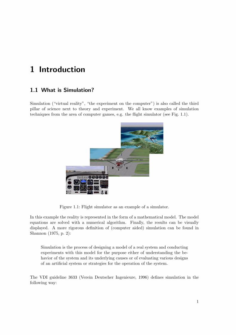
Simulation (“virtual reality”, “the experiment on the computer”) is also called the thirdpillar of science next to theory and experiment. We all know examples of simulationtechniques from the area of computer games, e.g. the flight simulator (see Fig. 1.1).
Figure 1.1: Flight simulator as an example of a simulator.
In this example the reality is represented in the form of a mathematical model. The modelequations are solved with a numerical algorithm. Finally, the results can be visuallydisplayed. A more rigorous definition of (computer aided) simulation can be found inShannon (1975, p. 2):
Simulation is the process of designing a model of a real system and conductingexperiments with this model for the purpose either of understanding the be-havior of the system and its underlying causes or of evaluating various designsof an artificial system or strategies for the operation of the system.
The VDI guideline 3633 (Verein Deutscher Ingenieure, 1996) defines simulation in thefollowing way:
1
1 Introduction
Simulation is the process of emulating a system with its dynamic processesin an experimental model in order to receive some knowledge, which is trans-ferable to the reality.In a broader sense, simulation means the preparation, the execution, and theevaluation of aimed experiments by means of a simulation model.With the help of simulation the temporal behavior of complex systems can bediscovered (simulation method).
Examples of application areas where simulation studies are used are:
flight simulators,
weather forecast,
stock market,
war gaming,
software development,
flexible manufacturing,
chemical processes,
power plants.
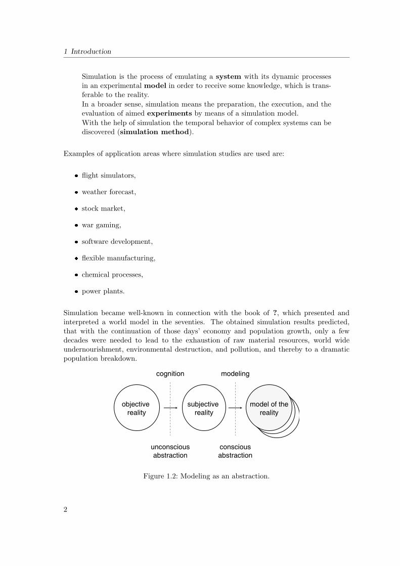
Simulation became well-known in connection with the book of ?, which presented andinterpreted a world model in the seventies. The obtained simulation results predicted,that with the continuation of those days’ economy and population growth, only a fewdecades were needed to lead to the exhaustion of raw material resources, world wideundernourishment, environmental destruction, and pollution, and thereby to a dramaticpopulation breakdown.
Figure 1.2: Modeling as an abstraction.
2
1.1 What is Simulation?
As Fig. 1.2 shows, you should be aware of the differences between reality and its represen-tation by the computer. This is because modeling is an intended simplification of realitythrough abstraction.
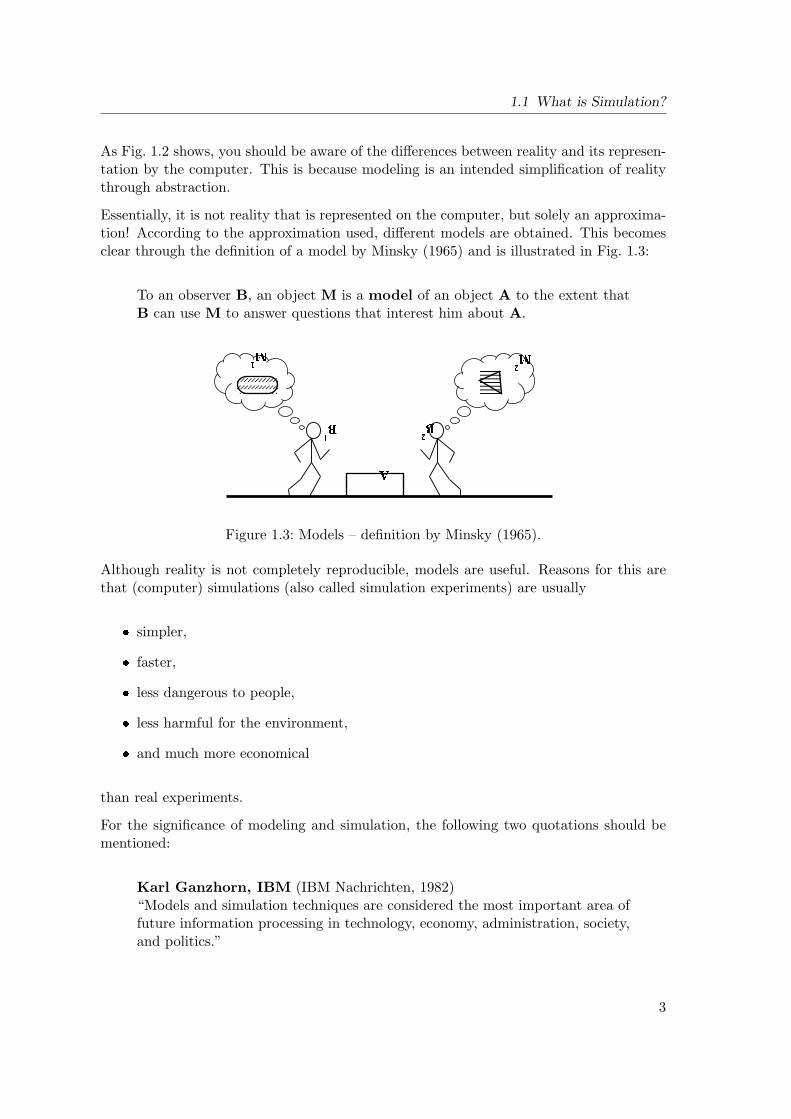
Essentially, it is not reality that is represented on the computer, but solely an approxima-tion! According to the approximation used, different models are obtained. This becomesclear through the definition of a model by Minsky (1965) and is illustrated in Fig. 1.3:
To an observer B, an object M is a model of an object A to the extent thatB can use M to answer questions that interest him about A.
Figure 1.3: Models – definition by Minsky (1965).
Although reality is not completely reproducible, models are useful. Reasons for this arethat (computer) simulations (also called simulation experiments) are usually
simpler,
faster,
less dangerous to people,
less harmful for the environment,
and much more economical
than real experiments.
For the significance of modeling and simulation, the following two quotations should bementioned:
Karl Ganzhorn, IBM (IBM Nachrichten, 1982)“Models and simulation techniques are considered the most important area offuture information processing in technology, economy, administration, society,and politics.”
3
1 Introduction
Ralph P. Schlenker, Exxon (Conference of Foundations of Computer-AidedProcess Operations, 1987)“Modeling and simulation technology are keys to achieve manufacturing excel-lence and to assess risk in unit operation. [...] As we make our plant operationsmore flexible to respond to business opportunities, efficient modeling and sim-ulation techniques will become commonly used tools.”
1.2 Simulation Procedure
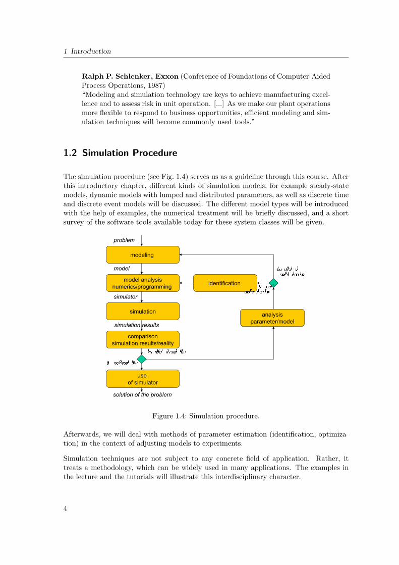
The simulation procedure (see Fig. 1.4) serves us as a guideline through this course. Afterthis introductory chapter, different kinds of simulation models, for example steady-statemodels, dynamic models with lumped and distributed parameters, as well as discrete timeand discrete event models will be discussed. The different model types will be introducedwith the help of examples, the numerical treatment will be briefly discussed, and a shortsurvey of the software tools available today for these system classes will be given.
Figure 1.4: Simulation procedure.
Afterwards, we will deal with methods of parameter estimation (identification, optimiza-tion) in the context of adjusting models to experiments.
Simulation techniques are not subject to any concrete field of application. Rather, ittreats a methodology, which can be widely used in many applications. The examples inthe lecture and the tutorials will illustrate this interdisciplinary character.
4
1.3 Introductory Example for the Simulation Procedure
1.3 Introductory Example for the Simulation Procedure
For illustration purposes, the following example is presented, in which the main steps inthe simulation procedure are mentioned.
1.3.1 Problem
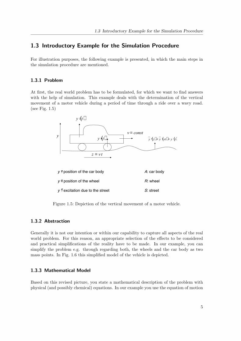
At first, the real world problem has to be formulated, for which we want to find answerswith the help of simulation. This example deals with the determination of the verticalmovement of a motor vehicle during a period of time through a ride over a wavy road.(see Fig. 1.5)
( )
( ) ( ) ( ) ( ) ==
=
=
Figure 1.5: Depiction of the vertical movement of a motor vehicle.
1.3.2 Abstraction
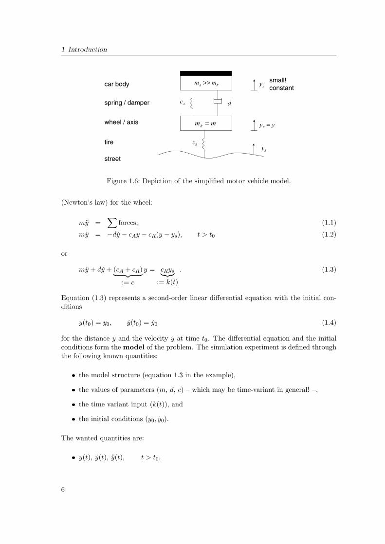
Generally it is not our intention or within our capability to capture all aspects of the realworld problem. For this reason, an appropriate selection of the effects to be consideredand practical simplifications of the reality have to be made. In our example, you cansimplify the problem e.g. through regarding both, the wheels and the car body as twomass points. In Fig. 1.6 this simplified model of the vehicle is depicted.
1.3.3 Mathematical Model
Based on this revised picture, you state a mathematical description of the problem withphysical (and possibly chemical) equations. In our example you use the equation of motion
5
1 Introduction1 Introduction
>>
=
=
Figure 1.6: Depiction of the simplified motor vehicle model.
(Newton’s law) for the wheel:
my =∑
forces, (1.1)
my = −dy − cAy − cR(y − ys), t > t0 (1.2)
or
my + dy + (cA + cR)︸ ︷︷ ︸:= c
y = cRys︸︷︷︸:= k(t)
. (1.3)
(1.3) represents a second-order linear differential equation with the initial conditions
y(t0) = y0, y(t0) = y0 (1.4)
for the distance y and the velocity y at time t0. The differential equation and the initialconditions form the model of the problem. The simulation experiment is defined throughthe following known quantities:
model structure,
(time variant!) parameter (m, d, c),
(time variant!) input k(t) and the
initial conditions y0, y0.
The wanted quantities are:
y(t), y(t), y(t), t > t0.
6
Figure 1.6: Depiction of the simplified motor vehicle model.
(Newton’s law) for the wheel:
my =∑
forces, (1.1)
my = −dy − cAy − cR(y − ys), t > t0 (1.2)
or
my + dy + (cA + cR)︸ ︷︷ ︸:= c
y = cRys︸︷︷︸:= k(t)
. (1.3)
Equation (1.3) represents a second-order linear differential equation with the initial con-ditions
y(t0) = y0, y(t0) = y0 (1.4)
for the distance y and the velocity y at time t0. The differential equation and the initialconditions form the model of the problem. The simulation experiment is defined throughthe following known quantities:
the model structure (equation 1.3 in the example),
the values of parameters (m, d, c) – which may be time-variant in general! –,
the time variant input (k(t)), and
the initial conditions (y0, y0).
The wanted quantities are:
y(t), y(t), y(t), t > t0.
6
1.3 Introductory Example for the Simulation Procedure
1.3.4 Simulation Model
For simulation purposes, you often do not rely on the model as it has been built throughabstraction (which are in our example the equations (1.3) and (1.4)). Rather, you docertain conversions on it. In this example, the conversion would result in a system offirst-order differential equations (so called state description). The states correspond toenergy storages, characterized by the according initial conditions. We define the variables:
x1 = y distance, (1.5)x2 = y velocity, (1.6)
which leads to the following differential equations:
x1 =dx1
dt= y = x2 , x1(t0) = y0 , (1.7)
x2 =dx2
dt= y =
1m
(−dx2 − cx1 + k(t)) , x2(t0) = y0 . (1.8)
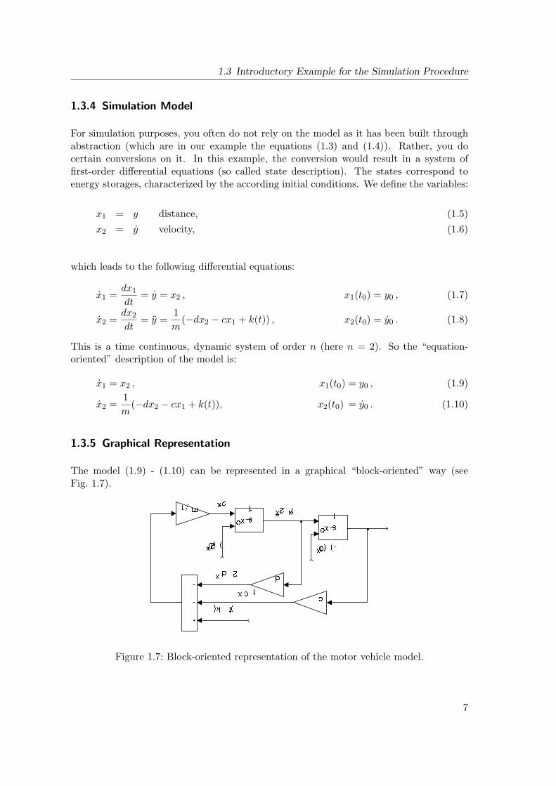
This is a time continuous, dynamic system of order n (here n = 2). So the “equation-oriented” description of the model is:
x1 = x2 , x1(t0) = y0 , (1.9)
x2 =1m
(−dx2 − cx1 + k(t)), x2(t0) = y0 . (1.10)
1.3.5 Graphical Representation
The model (1.9) - (1.10) can be represented in a graphical “block-oriented” way (seeFig. 1.7).
! "# $
%& ' (
) * +, -
Figure 1.7: Block-oriented representation of the motor vehicle model.
7
1 Introduction
1.3.6 Analysis of the Model
For preparation of a reasonable simulation, an analysis of the model is necessary, e.g. inview of the following points:
a. WellposednessThe problem must have definite solutions for all meaningful values of parameters, in-puts, and initial conditions (see existence theorem for first-order differential equationsystems in Section 3.2).
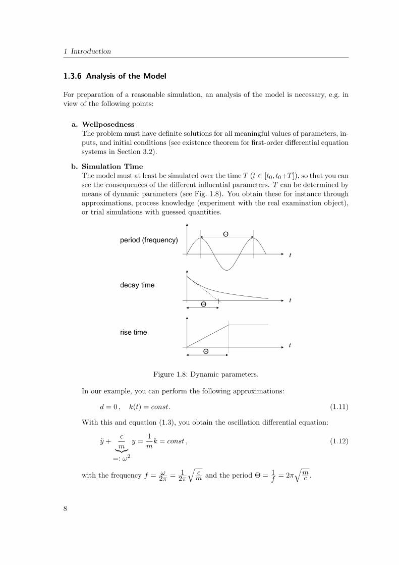
b. Simulation TimeThe model must at least be simulated over the time T (t ∈ [t0, t0+T ]), so that you cansee the consequences of the different influential parameters. T can be determined bymeans of dynamic parameters (see Fig. 1.8). You obtain these for instance throughapproximations, process knowledge (experiment with the real examination object),or trial simulations with guessed quantities.
Θ
Θ
Θ
Figure 1.8: Dynamic parameters.
In our example, you can perform the following approximations:
d = 0 , k(t) = const. (1.11)
With this and equation (1.3), you obtain the oscillation differential equation:
y +c
m︸︷︷︸=: ω2
y =1m
k = const , (1.12)
with the frequency f = ω2π = 1
2π
√cm and the period Θ = 1
f= 2π
√mc .
8
1.3 Introductory Example for the Simulation Procedure
A model is characterized through the time parameters Tmax and Tmin:
Tmax = max( period︸ ︷︷ ︸Θ as above
, excitation︸ ︷︷ ︸typical time
for the characterization
of k(t)
), (1.13)
Tmin = min(period, excitation). (1.14)
As an empirical formula, the simulation time T can be determined by:
T = 5 · Tmax (1.15)
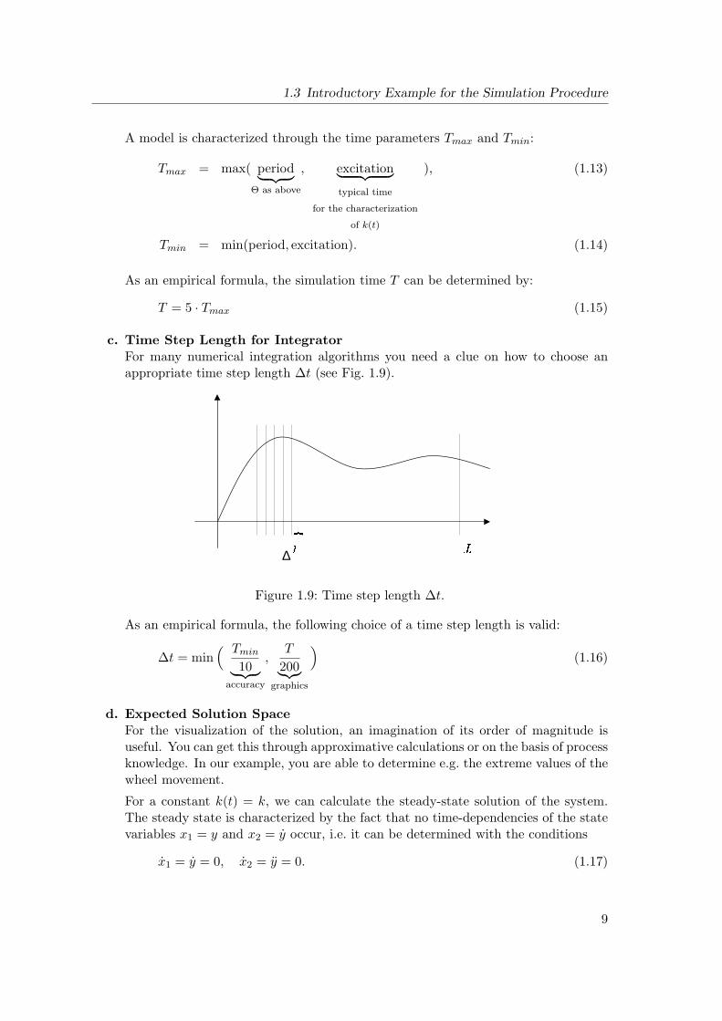
c. Time Step Length for IntegratorFor many numerical integration algorithms you need a clue on how to choose anappropriate time step length ∆t (see Fig. 1.9).
∆
Figure 1.9: Time step length ∆t.
As an empirical formula, the following choice of a time step length is valid:
∆t = min( Tmin
10︸ ︷︷ ︸accuracy
,T
200︸︷︷︸graphics
)(1.16)
d. Expected Solution SpaceFor the visualization of the solution, an imagination of its order of magnitude isuseful. You can get this through approximative calculations or on the basis of processknowledge. In our example, you are able to determine e.g. the extreme values of thewheel movement.
For a constant k(t) = k, we can calculate the steady-state solution of the system.The steady state is characterized by the fact that no time-dependencies of the statevariables x1 = y and x2 = y occur, i.e. it can be determined with the conditions
x1 = y = 0, x2 = y = 0. (1.17)
9
1 Introduction
Then equation (1.3) yields an expression for the steady-state solution y:
cy = k, (1.18)
hence
y =k
c. (1.19)
The dynamic solution of equation (1.3) is given by (assuming d = 0):
y(t) = x1(t) = y(1− cos(ωt)), (1.20)y(t) = x2(t) = y ω sin(ωt), (1.21)
therefore
x1,max = 2 y, x1,min = 0, (1.22)x2,max = ω y, x2,min = −ω y. (1.23)
1.3.7 Numerical Solution
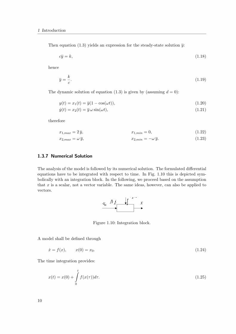
The analysis of the model is followed by its numerical solution. The formulated differentialequations have to be integrated with respect to time. In Fig. 1.10 this is depicted sym-bolically with an integration block. In the following, we proceed based on the assumptionthat x is a scalar, not a vector variable. The same ideas, however, can also be applied tovectors.
=
Figure 1.10: Integration block.
A model shall be defined through
x = f(x), x(0) = x0. (1.24)
The time integration provides:
x(t) = x(0) +
t∫0
f(x(τ))dτ. (1.25)
10
1.3 Introductory Example for the Simulation Procedure
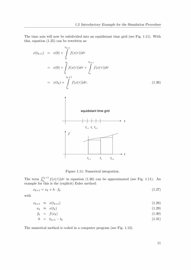
The time axis will now be subdivided into an equidistant time grid (see Fig. 1.11). Withthis, equation (1.25) can be rewritten as:
x(tk+1) = x(0) +
tk+1∫0
f(x(τ))dτ
= x(0) +
tk∫0
f(x(τ))dτ +
tk+1∫tk
f(x(τ))dτ
= x(tk) +
tk+1∫tk
f(x(τ))dτ. (1.26)
1.3 Introductory Example for the Simulation Procedure
−
+
−
+
Figure 1.11: Numerical integration.
The second term in (1.24) can be approximated (see Fig. 1.11). An example for this isthe (explicit) Euler method:
xk+1 = xk + h · fk (1.25)
with
xk+1 ≈ x(tk+1) (1.26)xk ≈ x(tk) (1.27)fk = f(xk) (1.28)h = tk+1 − tk (1.29)
Figure 1.11: Numerical integration.
The term∫ tk+1tk
f(x(τ))dτ in equation (1.26) can be approximated (see Fig. 1.11). Anexample for this is the (explicit) Euler method:
xk+1 = xk + h · fk (1.27)
with
xk+1 ≈ x(tk+1) (1.28)xk ≈ x(tk) (1.29)fk = f(xk) (1.30)h = tk+1 − tk (1.31)
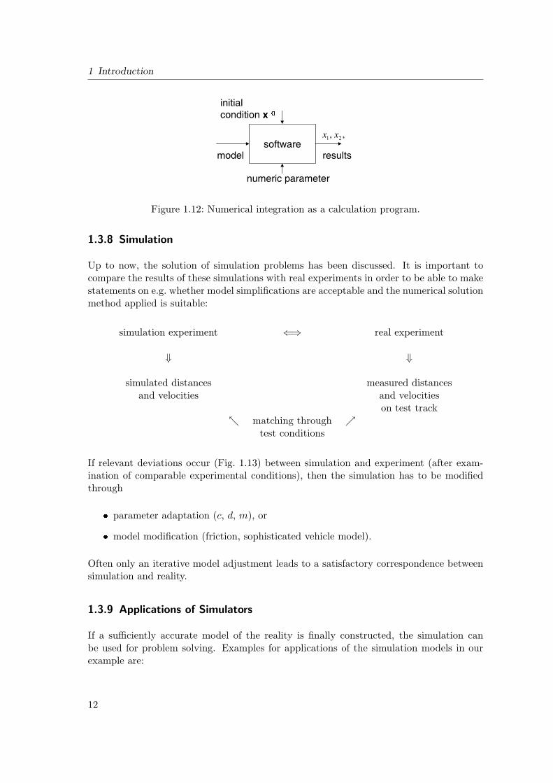
The numerical method is coded in a computer program (see Fig. 1.12).
11
1 Introduction
Figure 1.12: Numerical integration as a calculation program.
1.3.8 Simulation
Up to now, the solution of simulation problems has been discussed. It is important tocompare the results of these simulations with real experiments in order to be able to makestatements on e.g. whether model simplifications are acceptable and the numerical solutionmethod applied is suitable:
simulation experiment ⇐⇒ real experiment
⇓ ⇓
simulated distances measured distancesand velocities and velocities
on test track matching through
test conditions
If relevant deviations occur (Fig. 1.13) between simulation and experiment (after exam-ination of comparable experimental conditions), then the simulation has to be modifiedthrough
parameter adaptation (c, d, m), or
model modification (friction, sophisticated vehicle model).
Often only an iterative model adjustment leads to a satisfactory correspondence betweensimulation and reality.
1.3.9 Applications of Simulators
If a sufficiently accurate model of the reality is finally constructed, the simulation canbe used for problem solving. Examples for applications of the simulation models in ourexample are:
12
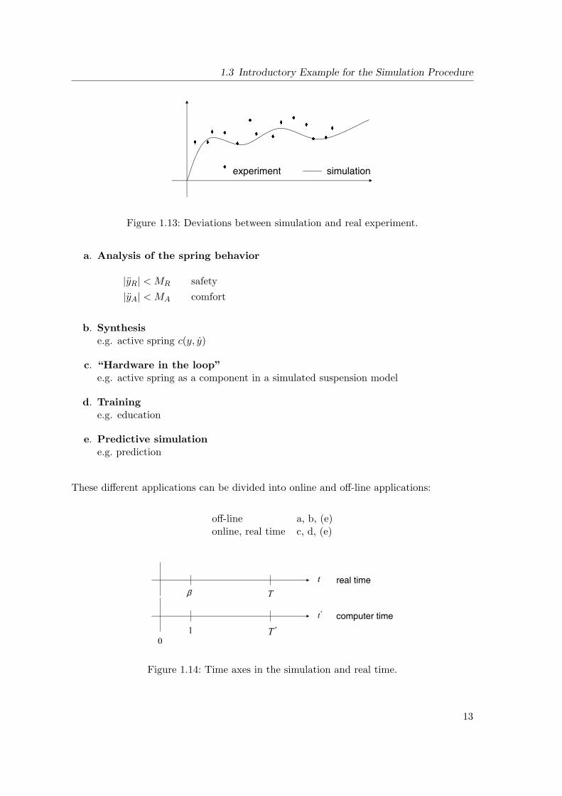
1.3 Introductory Example for the Simulation Procedure
Figure 1.13: Deviations between simulation and real experiment.
a. Analysis of the spring behavior
|yR| < MR safety|yA| < MA comfort
b. Synthesise.g. active spring c(y, y)
c. “Hardware in the loop”e.g. active spring as a component in a simulated suspension model
d. Traininge.g. education
e. Predictive simulatione.g. prediction
These different applications can be divided into online and off-line applications:
off-line a, b, (e)online, real time c, d, (e)
β
∗
∗
Figure 1.14: Time axes in the simulation and real time.
13
1 Introduction
On the basis of Fig. 1.14, simulation can be divided with regard to its time scales:
β =T
T ∗=
t
t∗
= 1 real time,< 1 time extension,> 1 time compression,
(1.32)
14
2 Representation of Dynamic Systems
2.1 State Representation of Linear Dynamic Systems
The example of the vertical movement of a motor vehicle in the previous chapter led to atime continuous dynamic system (with lumped parameters), which is described throughordinary differential equations with time as the independent variable. In this chapter wewill generalize this system representation. Starting with one or more linear differentialequations of higher order, we are going to implement a transformation such that we get asystem of differential equations of first order (Zeitz, 1999). This alternative representationof the model is useful for determining certain characteristics of the system in consideration,for instance its stability. Furthermore, as we will see in Chapter 5, common numericalintegration methods require a system of differential equations of first order.
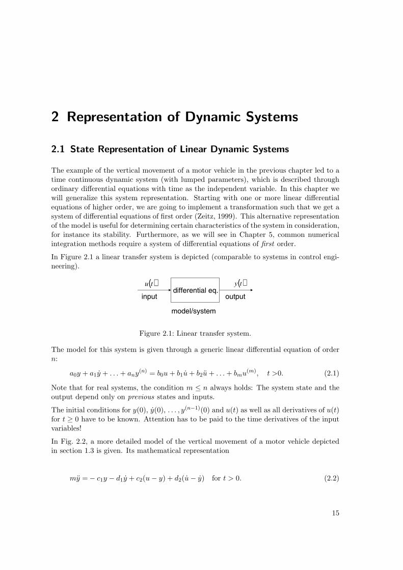
In Figure 2.1 a linear transfer system is depicted (comparable to systems in control engi-neering).
( ) ( )
Figure 2.1: Linear transfer system.
The model for this system is given through a generic linear differential equation of ordern:
a0y + a1y + . . . + any(n) = b0u + b1u + b2u + . . . + bmu(m), t >0. (2.1)
Note that for real systems, the condition m ≤ n always holds: The system state and theoutput depend only on previous states and inputs.
The initial conditions for y(0), y(0), . . . , y(n−1)(0) and u(t) as well as all derivatives of u(t)for t ≥ 0 have to be known. Attention has to be paid to the time derivatives of the inputvariables!
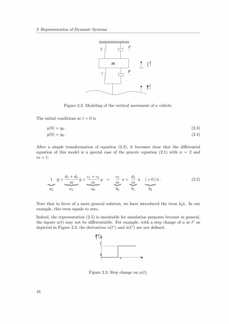
In Fig. 2.2, a more detailed model of the vertical movement of a motor vehicle depictedin section 1.3 is given. Its mathematical representation
my =− c1y − d1y + c2(u− y) + d2(u− y) for t > 0. (2.2)
15
2 Representation of Dynamic Systems
( )
( )
m
Figure 2.2: Modeling of the vertical movement of a vehicle.
The initial conditions at t = 0 is
y(0) = y0 , (2.3)y(0) = y0 . (2.4)
After a simple transformation of equation (2.2), it becomes clear that the differentialequation of this model is a special case of the generic equation (2.1) with n = 2 andm = 1:
1︸︷︷︸a2
·y +d1 + d2
m︸ ︷︷ ︸a1
y +c1 + c2
m︸ ︷︷ ︸a0
y =c2
m︸︷︷︸b0
u +d2
m︸︷︷︸b1
u ( + 0 )︸ ︷︷ ︸b2
u . (2.5)
Note that in favor of a more general solution, we have introduced the term b2u. In ourexample, this term equals to zero.
Indeed, the representation (2.5) is unsuitable for simulation purposes because in general,the inputs u(t) may not be differentiable. For example, with a step change of u at t∗ asdepicted in Figure 2.3, the derivatives u(t∗) and u(t∗) are not defined.
( )
Figure 2.3: Step change on u(t).
16
2.1 State Representation of Linear Dynamic Systems
As such discontinuities cause difficulties in simulation (i.e. in the numerical methods),equations like (2.1) are transformed through successive integration at time 0 in the intervalfrom t = 0 to t = 0+. As we want to eliminate all derivatives u, u, ..., u(m), m integrationsare required:
0+∫t=0
. . .
0+∫t=0
m integrals
differential equation dτ . . . dτ . (2.6)
Inspect, for instance, the general case n = m = 2 as in equation (2.5): By solving thisequation with respect to the highest order derivative in y you obtain
y = b0u− a0y + b1u− a1y + b2u (2.7)
with the initial conditions
y(0) = y0 , (2.8)y(0) = y0 . (2.9)
As equation (2.7) is of second order in u, two integrations are required to obtain a repre-sentation free of derivatives of u. After the first integration, we get
y(t) =∫
(b0u− a0y)︸ ︷︷ ︸=: x1
dτ + b1u− a1y + b2u , (2.10)
hence
y(t) = x1 + b1u− a1y + b2u , (2.11)
and the second integration yields
y(t) =∫
(x1 + b1u− a1y)︸ ︷︷ ︸=: x2
dτ + b2u
= x2 + b2u . (2.12)
We get the following equation system, consisting of two differential equations, namelythe definitions of x1 and x2 in equation (2.10) and (2.11) respectively, and one algebraicequation, i.e. equation (2.12):
x1 = b0u− a0y , (2.13)x2 = x1 + b1u− a1y , (2.14)y = x2 + b2u , (2.15)
17
2 Representation of Dynamic Systems
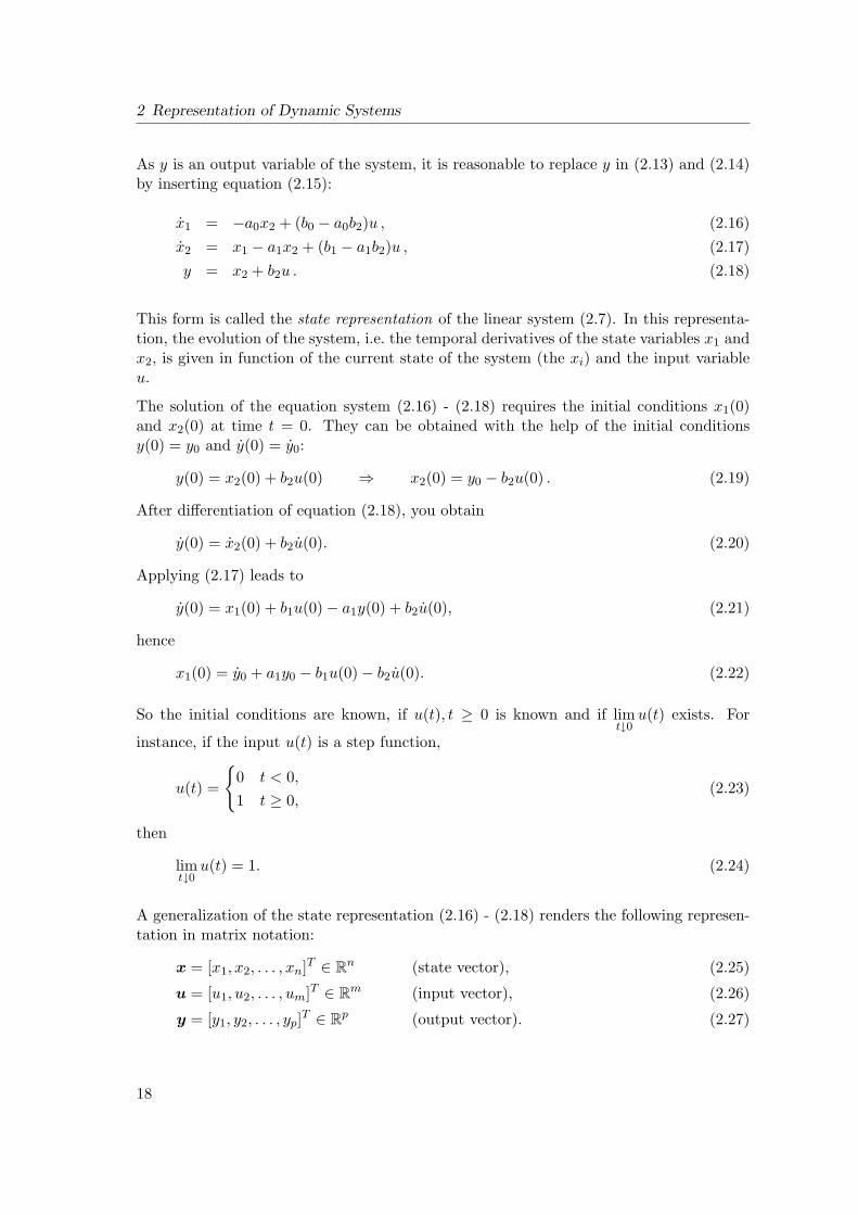
As y is an output variable of the system, it is reasonable to replace y in (2.13) and (2.14)by inserting equation (2.15):
x1 = −a0x2 + (b0 − a0b2)u , (2.16)x2 = x1 − a1x2 + (b1 − a1b2)u , (2.17)y = x2 + b2u . (2.18)
This form is called the state representation of the linear system (2.7). In this representa-tion, the evolution of the system, i.e. the temporal derivatives of the state variables x1 andx2, is given in function of the current state of the system (the xi) and the input variableu.
The solution of the equation system (2.16) - (2.18) requires the initial conditions x1(0)and x2(0) at time t = 0. They can be obtained with the help of the initial conditionsy(0) = y0 and y(0) = y0:
y(0) = x2(0) + b2u(0) ⇒ x2(0) = y0 − b2u(0) . (2.19)
After differentiation of equation (2.18), you obtain
y(0) = x2(0) + b2u(0). (2.20)
Applying (2.17) leads to
y(0) = x1(0) + b1u(0)− a1y(0) + b2u(0), (2.21)
hence
x1(0) = y0 + a1y0 − b1u(0)− b2u(0). (2.22)
So the initial conditions are known, if u(t), t ≥ 0 is known and if limt↓0
u(t) exists. For
instance, if the input u(t) is a step function,
u(t) =
0 t < 0,
1 t ≥ 0,(2.23)
then
limt↓0
u(t) = 1. (2.24)
A generalization of the state representation (2.16) - (2.18) renders the following represen-tation in matrix notation:
x = [x1, x2, . . . , xn]T ∈ Rn (state vector), (2.25)
u = [u1, u2, . . . , um]T ∈ Rm (input vector), (2.26)
y = [y1, y2, . . . , yp]T ∈ Rp (output vector). (2.27)
18
2.2 The State Space
In our example this means:[x1
x2
]︸︷︷︸
x
=[0 −a0
1 −a1
]︸ ︷︷ ︸
A
[x1
x2
]︸︷︷︸
x
+[b0 − a0b2
b1 − a1b2
]︸ ︷︷ ︸
B
u︸︷︷︸u
(2.28)
system matrix input matrixn× n n× 1 n×m m× 1
y︸︷︷︸y
=[0 1
]︸ ︷︷ ︸
C
[x1
x2
]︸︷︷︸
x
+ b2︸︷︷︸D
u︸︷︷︸u
(2.29)
output matrix transmission matrixp× n n× 1 p×m m× 1
Therefore, you obtain a generic linear state representation in the following form:
x = Ax + Bu, x(0) = x0, (2.30)y = Cx + Du. (2.31)
Consequently, the simulation task is to solve a system of linear differential equations offirst order.
2.2 The State Space
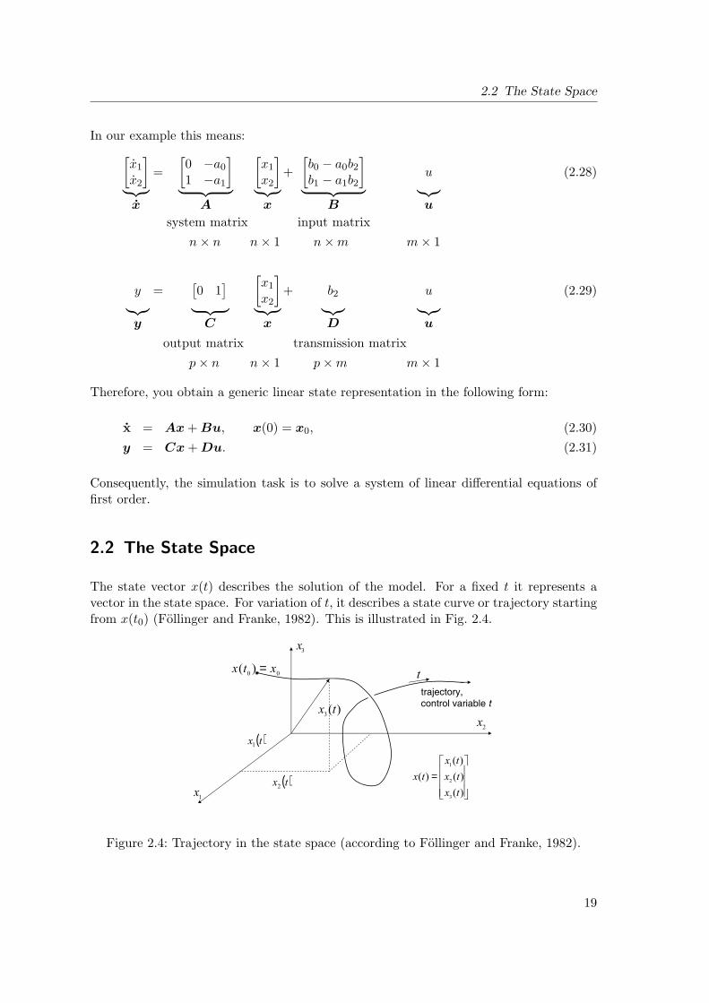
The state vector x(t) describes the solution of the model. For a fixed t it represents avector in the state space. For variation of t, it describes a state curve or trajectory startingfrom x(t0) (Follinger and Franke, 1982). This is illustrated in Fig. 2.4.
2.2 The State Space
2.2 The State Space
The state vector x(t) describes the solution of the model. For a fixed t it represents avector in the state space. For variation of t, it describes a state curve or trajectory startingfrom x(t0) (Follinger and Franke, 1982). This is illustrated in Fig. 2.4.
( )
=
( )
=
Figure 2.4: Trajectory in the state space (according to Follinger and Franke, 1982).
For given inputs u(t), t ≥ t0, the trajectory is definitely determined through the initialconditions x(t0) = x0. For different u(t) with the same x0, you obtain different trajectories.
The special case n = 2 (two-dimensional state space) is illustrated in Fig. 2.5, left. Thisillustration is also called phase plot. Fig. 2.5, right, shows in contrast a time domaindepiction.
( )
Figure 2.5: Phase plot and time domain depiction.
2.3 State Representation of Nonlinear Dynamic Systems
Most real systems cannot be sufficiently represented with linear relations. Therefore, weextend the state representation to the nonlinear case (Follinger and Franke, 1982; Zeitz,1999).
19
Figure 2.4: Trajectory in the state space (according to Follinger and Franke, 1982).
19
2 Representation of Dynamic Systems
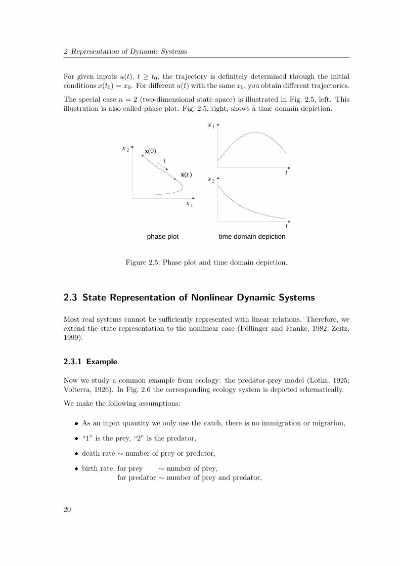
For given inputs u(t), t ≥ t0, the trajectory is definitely determined through the initialconditions x(t0) = x0. For different u(t) with the same x0, you obtain different trajectories.
The special case n = 2 (two-dimensional state space) is illustrated in Fig. 2.5, left. Thisillustration is also called phase plot. Fig. 2.5, right, shows a time domain depiction.
phase plot time domain depiction
t
x(0)
x(t ) t
t
x 1
x 2
x 2
x 1
Figure 2.5: Phase plot and time domain depiction.
2.3 State Representation of Nonlinear Dynamic Systems
Most real systems cannot be sufficiently represented with linear relations. Therefore, weextend the state representation to the nonlinear case (Follinger and Franke, 1982; Zeitz,1999).
2.3.1 Example
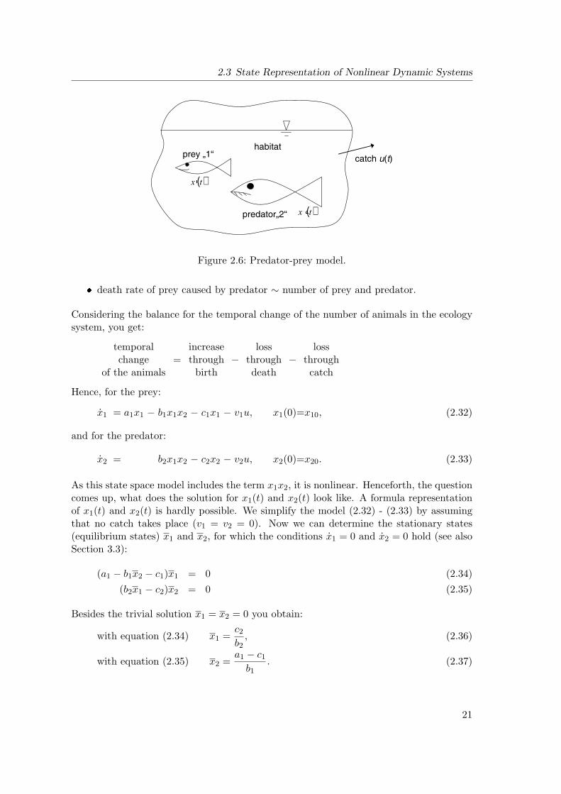
Now we study a common example from ecology: the predator-prey model (Lotka, 1925;Volterra, 1926). In Fig. 2.6 the corresponding ecology system is depicted schematically.
We make the following assumptions:
As an input quantity we only use the catch, there is no immigration or migration,
“1” is the prey, “2” is the predator,
death rate ∼ number of prey or predator,
birth rate, for prey ∼ number of prey,for predator ∼ number of prey and predator,
20
2.3 State Representation of Nonlinear Dynamic Systems
( )
( )
Figure 2.6: Predator-prey model.
death rate of prey caused by predator ∼ number of prey and predator.
Considering the balance for the temporal change of the number of animals in the ecologysystem, you get:
temporalchange
of the animals=
increasethroughbirth
−loss
throughdeath
−loss
throughcatch
Hence, for the prey:
x1 = a1x1 − b1x1x2 − c1x1 − v1u, x1(0)=x10, (2.32)
and for the predator:
x2 = b2x1x2 − c2x2 − v2u, x2(0)=x20. (2.33)
As this state space model includes the term x1x2, it is nonlinear. Henceforth, the questioncomes up, what does the solution for x1(t) and x2(t) look like. A formula representationof x1(t) and x2(t) is hardly possible. We simplify the model (2.32) - (2.33) by assumingthat no catch takes place (v1 = v2 = 0). Now we can determine the stationary states(equilibrium states) x1 and x2, for which the conditions x1 = 0 and x2 = 0 hold (see alsoSection 3.3):
(a1 − b1x2 − c1)x1 = 0 (2.34)(b2x1 − c2)x2 = 0 (2.35)
Besides the trivial solution x1 = x2 = 0 you obtain:
with equation (2.34) x1 =c2
b2, (2.36)
with equation (2.35) x2 =a1 − c1
b1. (2.37)
21
2 Representation of Dynamic Systems
In the following step the non-stationary solution trajectory has to be worked out. In thiscase you can use a trick, where you divide equation (2.33) by equation (2.32) and thenseparate the variables x1 and x2:
dx2/dt
dx1/dt=
dx2
dx1=
x2
a1 − b1x2 − c1· b2x1 − c2
x1, (2.38)
a1 − b1x2 − c1
x2dx2 =
b2x1 − c2
x1dx1, (2.39)
a1 − c1
x2dx2 − b1dx2 = b2dx1 −
c2
x1dx1, (2.40)
(a1 − c1) ln |x2| − b1x2 = b2x1 − c2 ln |x1|+ C. (2.41)
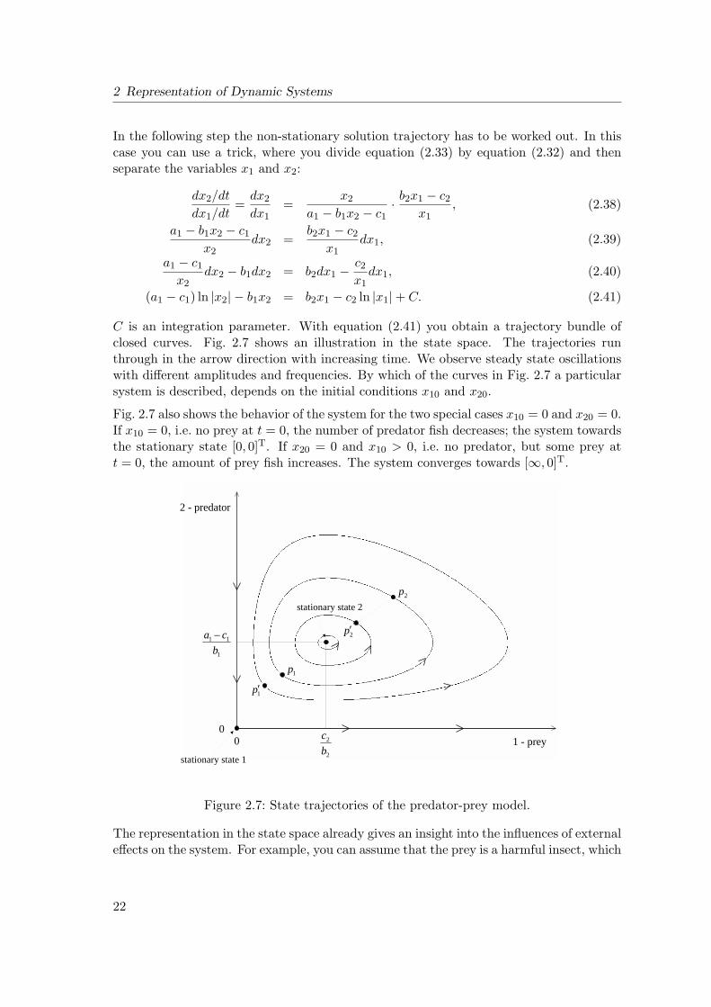
C is an integration parameter. With equation (2.41) you obtain a trajectory bundle ofclosed curves. Fig. 2.7 shows an illustration in the state space. The trajectories runthrough in the arrow direction with increasing time. We observe steady state oscillationswith different amplitudes and frequencies. By which of the curves in Fig. 2.7 a particularsystem is described, depends on the initial conditions x10 and x20.
Fig. 2.7 also shows the behavior of the system for the two special cases x10 = 0 and x20 = 0.If x10 = 0, i.e. no prey at t = 0, the number of predator fish decreases; the system towardsthe stationary state [0, 0]T. If x20 = 0 and x10 > 0, i.e. no predator, but some prey att = 0, the amount of prey fish increases. The system converges towards [∞, 0]T.
2
2
bc
1
11
bca −
00 1 - prey
2 - predator
stationary state 1
stationary state 22p
2p′
1p
1p′
Figure 2.7: State trajectories of the predator-prey model.
The representation in the state space already gives an insight into the influences of externaleffects on the system. For example, you can assume that the prey is a harmful insect, which
22
2.3 State Representation of Nonlinear Dynamic Systems
shall be reduced through the use of chemicals. Using chemicals to reduce the predator andthe prey from p1 to p′1 has the consequence that later a much greater amount of prey willappear. So a better time for combating would be a decisive moment with a large amountof prey, e.g. p2. An alternative would be a continuous intervention u(t). However, thiswould lead to the question of determining the optimal trajectory of u(t).
2.3.2 Generalized Representation
The general nonlinear state space model can be described in the following way:
x = f(x,u), x(0) = x0, (2.42)y = g(x,u). (2.43)
If f and g are both linear in the input quantity u, this leads to a so-called nonlinear,control affine state space model:
x = f1(x) + f2(x)u, x(0) = x0. (2.44)y = g1(x) + g2(x)u. (2.45)
So the simulation task consists of solving a system of nonlinear differential equations. Notethat you deal with a vector model:
x =
x1...
xn
, f =
f1...
fn
, . . . (2.46)
or x1...
xn
=
f1(x,u)...
fn(x,u)
,
x1(0)...
xn(0)
=
x10...
xn0
,
y1...yp
=
g1(x,u)...
gp(x,u)
. (2.47)
If the time t does not appear explicitly or implicitly through u(t) in the functions f andg, these systems are called autonomous.
Every non-autonomous system
x = f(x,u(t)) = f(x, t), (2.48)y = g(x,u(t)) = g(x, t) (2.49)
can be transformed into an autonomous one with the additional variable xn+1 = t and thesupplementary equation xn+1 = 1, xn+1(0) = 0.
23
2 Representation of Dynamic Systems
Example
For the non-autonomous system
y = ty, t > 0; y(0) = y0, (2.50)
we get with x1 := y, x2 := t:[x1
x2
]=
[x1x2
1
], t > 0;
[x1(0)x2(0)
]=
[y0
0
]. (2.51)
2.4 Block-Oriented Representation of Dynamic Systems
2.4.1 Block-Oriented Representation of Linear Systems
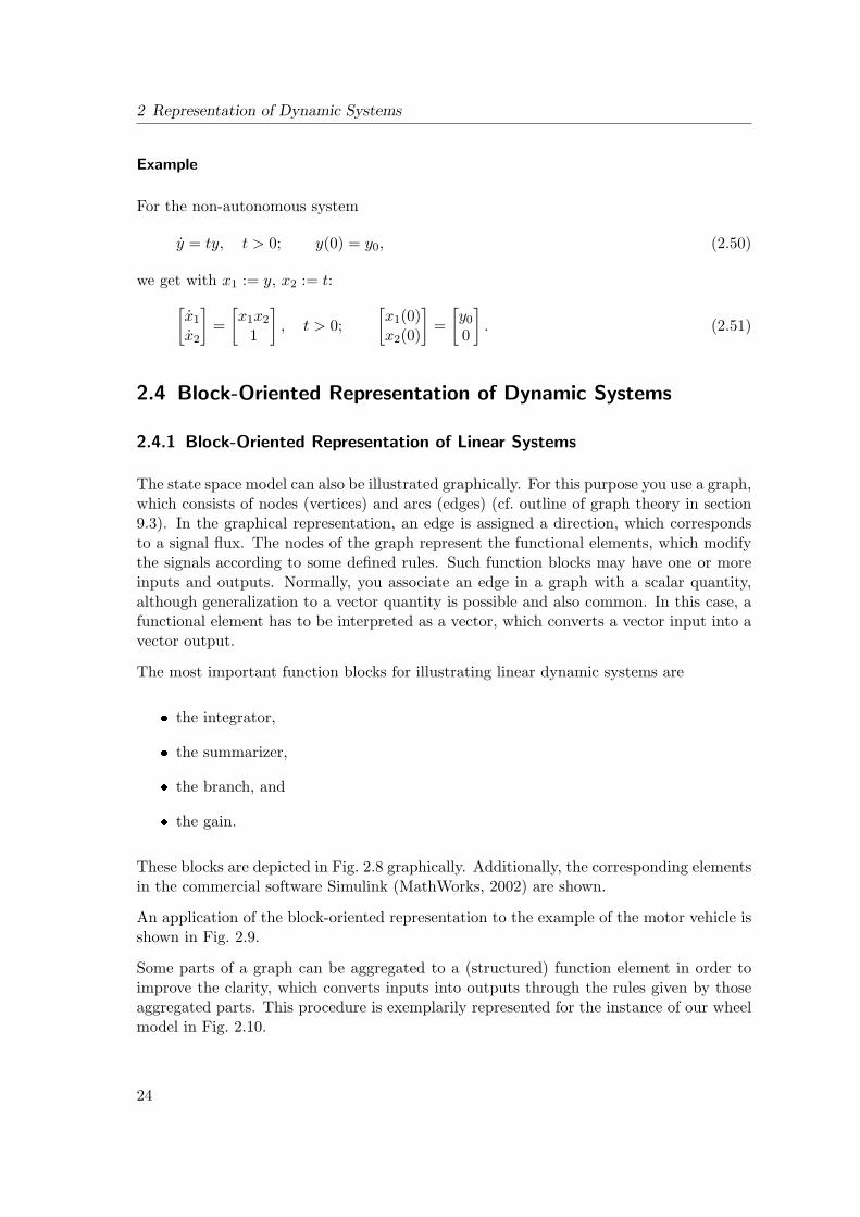
The state space model can also be illustrated graphically. For this purpose you use a graph,which consists of nodes (vertices) and arcs (edges) (cf. outline of graph theory in section9.3). In the graphical representation, an edge is assigned a direction, which correspondsto a signal flux. The nodes of the graph represent the functional elements, which modifythe signals according to some defined rules. Such function blocks may have one or moreinputs and outputs. Normally, you associate an edge in a graph with a scalar quantity,although generalization to a vector quantity is possible and also common. In this case, afunctional element has to be interpreted as a vector, which converts a vector input into avector output.
The most important function blocks for illustrating linear dynamic systems are
the integrator,
the summarizer,
the branch, and
the gain.
These blocks are depicted in Fig. 2.8 graphically. Additionally, the corresponding elementsin the commercial software Simulink (MathWorks, 2002) are shown.
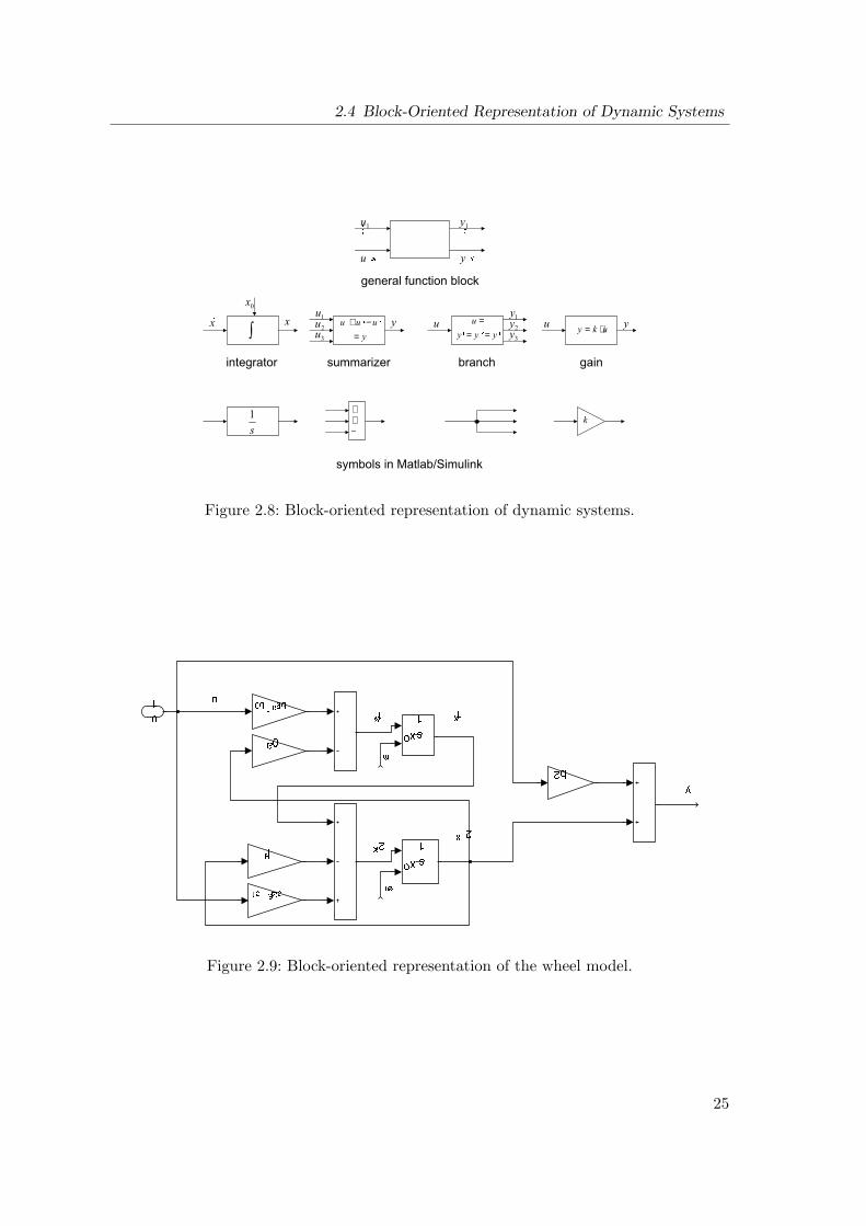
An application of the block-oriented representation to the example of the motor vehicle isshown in Fig. 2.9.
Some parts of a graph can be aggregated to a (structured) function element in order toimprove the clarity, which converts inputs into outputs through the rules given by thoseaggregated parts. This procedure is exemplarily represented for the instance of our wheelmodel in Fig. 2.10.
24
2.4 Block-Oriented Representation of Dynamic Systems
=−+
===
⋅=
++
−
Figure 2.8: Block-oriented representation of dynamic systems.
!"
# $
%&
' ()
*
+ ,-
. /0
Figure 2.9: Block-oriented representation of the wheel model.
25
2 Representation of Dynamic Systems
Figure 2.10: Aggregation of model parts.
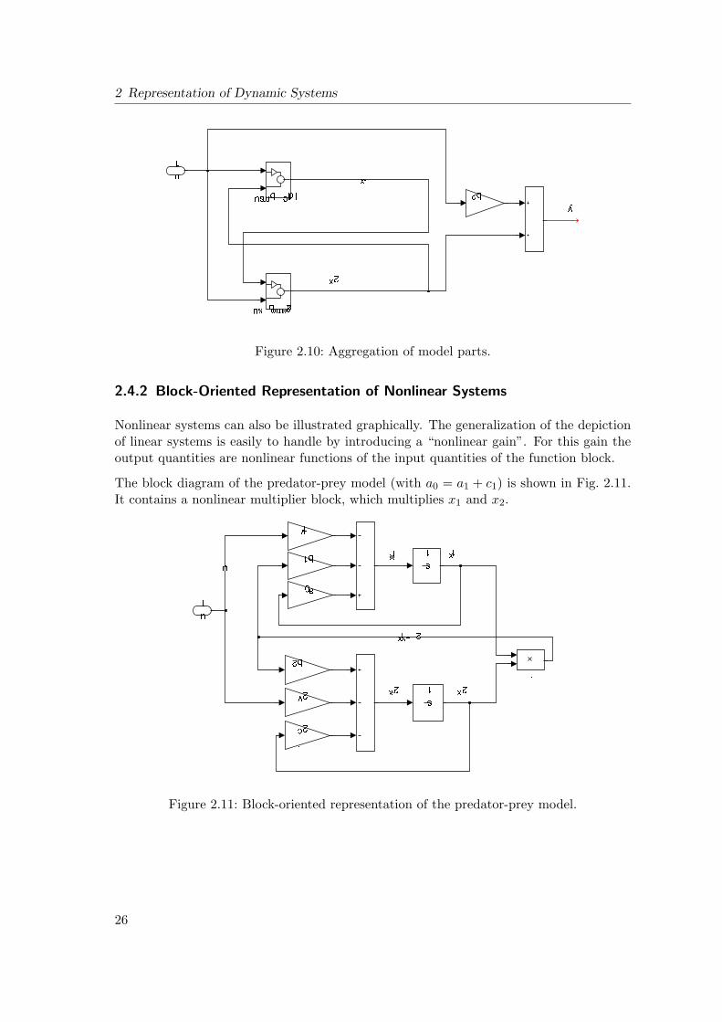
2.4.2 Block-Oriented Representation of Nonlinear Systems
Nonlinear systems can also be illustrated graphically. The generalization of the depictionof linear systems is easily to handle by introducing a “nonlinear gain”. For this gain theoutput quantities are nonlinear functions of the input quantities of the function block.
The block diagram of the predator-prey model (with a0 = a1 + c1) is shown in Fig. 2.11.It contains a nonlinear multiplier block, which multiplies x1 and x2.
!#" $
Figure 2.11: Block-oriented representation of the predator-prey model.
26
3 Model Analysis
Before solving the model equations a model analysis should be performed (see simulationprocedure, Fig. 1.4) in order to support the implementation of the model in a simulator.We look at an autonomous system of nonlinear differential equations of the form:
dx
dt= f(x), x(0) = x0. (3.1)
The output equations do not have to be considered because they are an explicit functionof states and inputs. Therefore, the outputs can also be determined after the simulation(which is normally not done for practical reasons). In the following sections, differentaspects of the model analysis will be briefly introduced.
3.1 Lipschitz continuity
Before we will discuss a criterion for the solvability of autonomous differential equations,we will introduce the term Lipschitz continuity. A function f : Rn → Rm is called Lipschitzcontinuous if a constant L > 0 exists such that for all x1,x2 ∈ Rn
‖f(x1)− f(x2)‖ ≤ L‖x1 − x2‖ . (3.2)
‖ · ‖ may be an arbitrary vector norm for Rm or Rn respectively, e.g. the maximum norm
‖x‖∞ = max1≤i≤n
xi (3.3)
or the Euclidean norm
‖x‖2 =1n
√x2
1 + ... + x2n. (3.4)
In general, continuity of a function is a necessary condition for Lipschitz continuity.
For differentiable functions, the following theorem is valid: A function f is Lipschitzcontinuous, if and only if its derivative is bounded, i.e. a constant L ∈ R exists such that
∀x ∈ Rn : ‖f ′(x)‖ ≤ L. (3.5)
27
3 Model Analysis
−2 −1 0 10
1
2
3
x
f(x)
(a) f(x) = e−x – not Lips-chitz continuous
−2 −1 0 1−4
−2
0
2
x
f(x)
(b) not continuous – notLipschitz continuous
−2 −1 0 10
1
2
3
x
f(x)
(c) f(x) = 1 + |x| – notdifferentiable, but Lipschitzcontinuous
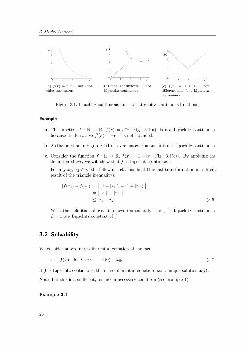
Figure 3.1: Lipschitz-continuous and non-Lipschitz-continuous functions.
Example
a. The function f : R → R, f(x) = e−x (Fig. 3.1(a)) is not Lipschitz continuous,because its derivative f ′(x) = −e−x is not bounded.
b. As the function in Figure 3.1(b) is even not continuous, it is not Lipschitz continuous.
c. Consider the function f : R → R, f(x) = 1 + |x| (Fig. 3.1(c)). By applying thedefinition above, we will show that f is Lipschitz continuous.
For any x1, x2 ∈ R, the following relations hold (the last transformation is a directresult of the triangle inequality):
|f(x1)− f(x2)| =∣∣ (1 + |x1|) − (1 + |x2|)
∣∣=
∣∣ |x1| − |x2|∣∣
≤ |x1 − x2|. (3.6)
With the definition above, it follows immediately that f is Lipschitz continuous;L = 1 is a Lipschitz constant of f .
3.2 Solvability
We consider an ordinary differential equation of the form
x = f(x) for t > 0 , x(0) = x0. (3.7)
If f is Lipschitz-continuous, then the differential equation has a unique solution x(t).
Note that this is a sufficient, but not a necessary condition (see example 1).
Example 3.1
28
3.2 Solvability
0 0.5 1 1.50
0.5
1
t
x(t)
(a) x = e−x, x(0) = 0
0 0.5 ln 2 1 1.5−1
−0.5
0
0.5
1
t
x(t)
(b) x = 1 + |x|, x(0) = −1
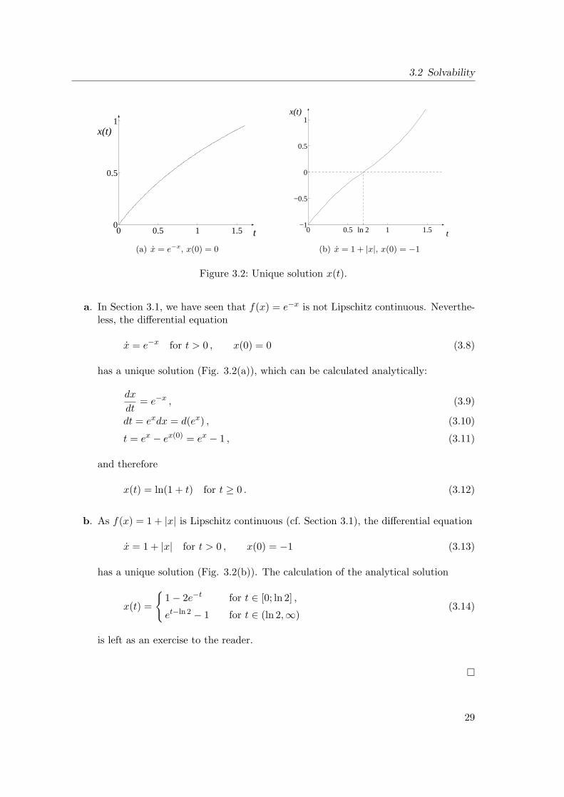
Figure 3.2: Unique solution x(t).
a. In Section 3.1, we have seen that f(x) = e−x is not Lipschitz continuous. Neverthe-less, the differential equation
x = e−x for t > 0 , x(0) = 0 (3.8)
has a unique solution (Fig. 3.2(a)), which can be calculated analytically:
dx
dt= e−x , (3.9)
dt = exdx = d(ex) , (3.10)
t = ex − ex(0) = ex − 1 , (3.11)
and therefore
x(t) = ln(1 + t) for t ≥ 0 . (3.12)
b. As f(x) = 1 + |x| is Lipschitz continuous (cf. Section 3.1), the differential equation
x = 1 + |x| for t > 0 , x(0) = −1 (3.13)
has a unique solution (Fig. 3.2(b)). The calculation of the analytical solution
x(t) =
1− 2e−t for t ∈ [0; ln 2] ,
et−ln 2 − 1 for t ∈ (ln 2,∞)(3.14)
is left as an exercise to the reader.
29
3 Model Analysis
3.3 Stationary States
In addition to the possible existence of a dynamic, i.e. time-dependent solution, the ques-tion of whether a system provides one or more stationary (steady) states is of interest. Bydefinition, a stationary state is characterized by the fact that the state variables x ∈ Rn
of a system
x = f(x,u) for t > 0 , (3.15)x(0) = x0 (3.16)
are constant with respect to time:
x = 0 . (3.17)
Therefore, for a given input u, the stationary states x of a system can be calculated bysolving the equation
f(x,u) = 0 . (3.18)
This condition shows that the stationary states of a system do not depend on initial values;they are a property of the system itself. Nevertheless, in general it depends on the initialvalues x(0) to which stationary state a system converges and whether it converges at all.
Example
In Section 2.3.1 we have seen that the predator-prey model has two stationary states:
x1 =[00
], x2 =
[ x2b2
a1−c1b1
]. (3.19)
If x(0) = x1 or x(0) = x2, then the system will remain in the respective stationarystate.
If x1(0) = 0 and x2(0) > 0, then the system will converge towards x1, but it willnever reach this state.
If x2(0) = 0 and x1(0) > 0, then the system will converge towards [∞, 0]T.
For all other x(0) with x1(0) > 0, x2(0) > 0, the system does not converge towardsa stationary state, but it follows the trajectories shown in Fig. 2.7.
For the calculation of stationary states, the linear and the nonlinear case are to be distin-guished:
30
3.4 Jacobian Matrix
linear case (x = Ax + Bu):
A x = −B u (3.20)
If the rank of the matrix rank(A) = n, i.e. detA 6= 0, then for any input u a solutionx such that A x + B u = 0 exists.
nonlinear case (x = f(x,u)):In the nonlinear case no sufficient conditions exist. As a necessary condition theimplicit function theorem
det∂f
∂x︸︷︷︸Jacobian
matrix
6= 0 if ||x− x|| < ε. (3.21)
has to be satisfied. The Jacobian matrix must have full rank for all x in the neigh-borhood of the searched stationary state x.
3.4 Jacobian Matrix
The Jacobian matrix of a differential equation system is defined in the following way:
∂f
∂x=
[∂fi
∂xj
]i,j=1,...,n
=
∂f1
∂x1. . .
∂f1
∂xn...
. . ....
∂fn
∂x1. . .
∂fn
∂xn
. (3.22)
Its calculation can be done either
analytically, e.g. manually or by a computer algebra system such as Maple or Math-ematica, or
numerically:
∂fi
∂xj≈ fi(. . . , xj + ∆xj , . . . )− fi(. . . , xj −∆xj , . . . )
2∆xj(3.23)
31
3 Model Analysis
The pattern of the Jacobian-Matrix reflects the coupling structure of the differential equa-tion system. Take a look at the following example; a non-zero entry is marked by ×:
∂f
∂x=
x1 x2 x3 x4 x50 × 0 × 00 × × 0 0...0 × × 0 ×
f1
f2
...f5
↓ ↓∂fi∂xj
6=0 =0
In this example, the function f1 depends only on x2 and x4. You distinguish betweendense (much more non-zero than zero entries) and sparse (much more zero entries) matri-ces. Among other reasons, this is important for the storage as well as for the numericalevaluation of the matrices (sparse numerical methods).
3.5 Linearization of Real Functions
The Taylor expansion of a function f : R → R at x is1
f(x) =∞∑i=0
1i!
dif
dxi
∣∣∣x=x
· (x− x)i (3.24)
= f(x) +df
dx
∣∣∣x=x
(x− x) +12
d2f
dx2
∣∣∣x=x
(x− x)2 + ... (3.25)
If the Taylor expansion is truncated after the second (linear) term, we get the a linearapproximation of f at x:
flin,x(x) = f(x) +df
dx
∣∣∣x=x
(x− x) . (3.26)
If ∆x := x− x is sufficiently small, then flin,x(x) ≈ f(x).
Note that a linearization of a function requires differentiability of the function at therespective point. In particular, a function cannot be linearized at saltuses or breakpoints(cf. Fig. 3.3).
Example
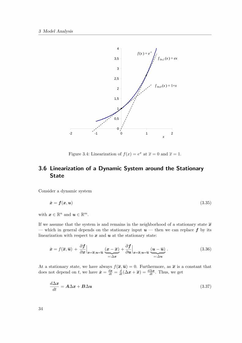
Let f(x) = ex. The linearization of f at x is
flin,x(x) = ex +( d
dxex
)x=x
· (x− x) (3.27)
= ex + ex · (x− x) (3.28)
= ex · (1− x + x) . (3.29)1 df
dx
x=x
is the value of f ′ = dfdx
at x.
32
3.5 Linearization of Real Functions
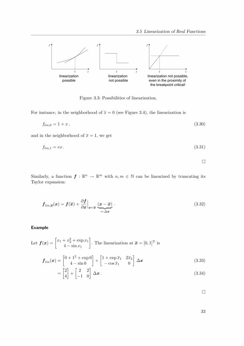
Figure 3.3: Possibilities of linearization.
For instance, in the neighborhood of x = 0 (see Figure 3.4), the linearization is
flin,0 = 1 + x , (3.30)
and in the neighborhood of x = 1, we get
flin,1 = ex . (3.31)
Similarly, a function f : Rn → Rm with n, m ∈ N can be linearized by truncating itsTaylor expansion:
f lin,x(x) = f(x) +∂f
∂x
∣∣∣x=x
(x− x)︸ ︷︷ ︸=:∆x
. (3.32)
Example
Let f(x) =[x1 + x2
2 + expx1
4− sin x1
]. The linearization at x = [0, 1]T is
f lin(x) =[0 + 12 + exp 0
4− sin 0
]+
[1 + expx1 2x2
− cos x1 0
]∆x (3.33)
=[24
]+
[2 2−1 0
]∆x . (3.34)
33
3 Model Analysis
0
0,5
1
1,5
2
2,5
3
3,5
4
-2 -1 0 1 2x
f (x ) = e x
f lin,0 (x ) = 1+x
f lin,1 (x ) = ex
Figure 3.4: Linearization of f(x) = ex at x = 0 and x = 1.
3.6 Linearization of a Dynamic System around the StationaryState
Consider a dynamic system
x = f(x,u) (3.35)
with x ∈ Rn and u ∈ Rm.
If we assume that the system is and remains in the neighborhood of a stationary state x— which in general depends on the stationary input u — then we can replace f by itslinearization with respect to x and u at the stationary state:
x = f(x,u) +∂f
∂x
∣∣∣x=x,u=u
(x− x)︸ ︷︷ ︸=:∆x
+∂f
∂u
∣∣∣x=x,u=u
(u− u)︸ ︷︷ ︸=:∆u
. (3.36)
At a stationary state, we have always f(x,u) = 0. Furthermore, as x is a constant thatdoes not depend on t, we have x = dx
dt = ddt(∆x + x) = d∆x
dt . Thus, we get
d∆x
dt= A∆x + B∆u (3.37)
34
3.7 Eigenvalues and eigenvectors
with
A =∂f
∂x
∣∣∣x=x,u=u
=
∂f1
∂x1
∂f1
∂x2. . .
∂f1
∂xn...
∂fn
∂x1
∂fn
∂x2. . .
∂fn
∂xn
x=x,u=u
(3.38)
and
B =∂f
∂u
∣∣∣x=x,u=u
=
∂f1
∂u1
∂f1
∂u2. . .
∂f1
∂um...
∂fn
∂u1
∂fn
∂u2. . .
∂fn
∂um
x=x,u=u
. (3.39)
The system matrix A is an n× n-matrix, the input matrix B is an n×m-matrix.
3.7 Eigenvalues and eigenvectors
For a given matrix A ∈ Cn×n, λ ∈ C and v ∈ Cn, v 6= 0 are called an eigenvalue and aneigenvector of A if the following equation holds:
Av = λv . (3.40)
In order to calculate the eigenvalues of a matrix, we transform equation (3.40):
(λI −A)v = 0 . (3.41)
Here, I denotes the n-dimensional identity matrix. As v 6= 0, equation (3.41) holds if andonly if
det(λI −A) = 0 . (3.42)
det(λI −A) is the characteristic polynomial of A.
Example
Let
A =
1 0 −10 1 −10 1 1
. (3.43)
35
3 Model Analysis
The characteristic polynomial of A is
det(λI −A) = det
λ− 1 0 10 λ− 1 10 −1 λ− 1
= (λ− 1)3 + (λ− 1)
= (λ− 1) [ (λ− 1)2 + 1 ] , (3.44)
and its roots are λ1 = 1, λ2 = 1 + i, and λ3 = 1− i.
3.8 Stability
A further important issue in the model analysis is the stability of a system after a pertur-bation ∆x0 of a stationary state x. In order to make statements about the stability of asystem, we will solve the homogeneous differential equation system (3.37) under the as-sumption that there are no perturbations of the input variables, i.e. ∆u = 0. Furthermore,we simplify the notation by writing x instead of ∆ x. Then equation (3.37) becomes
x = Ax , x(0) = x0 . (3.45)
A ∈ Rn×n is an n× n-matrix, where n is the number of state variables xi.
Assume that v ∈ Cn is an eigenvector of A and that λ is the corresponding eigenvalue,i.e.
Av = λv . (3.46)
It is evident that
x(t) = veλt (3.47)
is a solution of x = Ax, because
d
dtveλt = λveλt = Aveλt . (3.48)
It becomes obvious that the eigenvalues of A provide valuable information about thedynamic behavior of the system.
3.8.1 One state variable
In the simplest case, the system has only one state variable x = x1, i.e. n = 1 and A = [k].Note that k is the eigenvalue of A. The system is described by the scalar differentialequation
x = kx , x(0) = x0 , (3.49)
36
3.8 Stability
which has the solution
x(t) = x0 ekt . (3.50)
According to the value of k, the following statements about the system’s stability can bemade:
If k < 0, then limt→∞ x(t) = 0. Hence, the system will return to its stationary stateafter a (small) perturbation. The system is stable.
If k > 0 (and x0 6= 0), then |limt→∞ x(t)| = ∞. The system will not return to thestationary state; rather, the absolute value of the state variable x grows towardsinfinity. The system is unstable.
For k = 0, the system is said to be “on the limit of stability”.
3.8.2 System matrix with real eigenvalues
Now let A ∈ Rn×n be a square matrix whose eigenvalues λi are all real,
λi ∈ R ∀i = 1, ..., n . (3.51)
It is known from linear algebra that a matrix T ∈ Rn×n, det(T ) 6= 0, exists, such that
T−1AT = diag λi =
λ1
. . .λn
= Λ . (3.52)
Λ is diagonal matrix whose entries are the eigenvalues of A. Now, the differential equation(3.45) can be transformed as follows:
x = Ax = A TT−1︸ ︷︷ ︸identity
x , (3.53)
T−1x = T−1ATT−1x = ΛT−1x . (3.54)
We apply a coordinate transformation to the state vector x and get a new state vector z:
z = T−1x ⇔ x = Tz . (3.55)
In terms of the transformed state vector, equation (3.54) yields the following differentialequation:
z = Λz (3.56)
or
zi = λizi ∀ i ∈ 1, ..., n . (3.57)
These are n independent differential equations, one for each of the transformed statevariables zi. Hence, for each zi the argumentation in Section 3.8.1 is valid. We get thefollowing criteria for the stability of the system:
37
3 Model Analysis
If all eigenvalues are negative, i.e. λi < 0∀ i ∈ 1, ..., n, then the system is stable.
If there is at least one positive eigenvalue, i.e. ∃i ∈ 1, ..., n : λi > 0, then thesystem is unstable.
3.8.3 Complex eigenvalues of a 2× 2 system matrix
Let A ∈ R2×2 be a matrix of the form
A =[a −bb a
], a, b 6= 0 . (3.58)
The eigenvalues are the roots of the characteristic polynomial
0 = det(A− λI) = (a− λ)2 + b2 , (3.59)
hence
λ+ = a + bi , λ− = a− bi . (3.60)
By equation (3.47) we get that the two components x1 and x2 of the solution x(t) arelinear combinations of
eλ+t = e(a+bi)t = eat [ cos(bt) + i sin(bt) ] (3.61)
and
eλ−t = e(a−bi)t = eat [ cos(bt) − i sin(bt) ] . (3.62)
Therefore, the real parts of x1 and x2 are oscillations of the frequency b/2π, which aredamped (for a < 0) or excited (for a > 0) by the factor eat. For the stability of the system,this means that
for a < 0, the system is stable, and
for a > 0, the system is unstable.
3.8.4 General case
Let A ∈ Rn×n be a matrix with k ∈ N0 real eigenvalues λreali and l ∈ N0 pairs of conjugate
complex eigenvalues λcom +j = aj + bj i, λcom−
j = aj − bj i. Then a matrix T ∈ Rn×n,det(T ) 6= 0, exists, such that
T−1AT−1 =
λreal1
. . .λreal
k
a1 −b1
b1 a1
. . .al −bl
bl al
(3.63)
38
3.8 Stability
Hence, by a similar consideration as in Section 3.8.2, we can reduce the general case tothe one-dimensional case with a real eigenvalue in Section 3.8.1 and the two-dimensionalcase with complex eigenvalues in Section 3.8.3.
As a condition for the stability of a system x = Ax, we get:
If all real eigenvalues of A are negative and if the real parts of all complex eigenvaluesof A are negative, then the system is stable.
If there is at least one positive real eigenvalue or at least one complex eigenvaluewith a positive real part, then the system is unstable.
If A has pairs of conjugate complex eigenvalues a± bi, then the system shows oscil-lations with frequency b/2π.
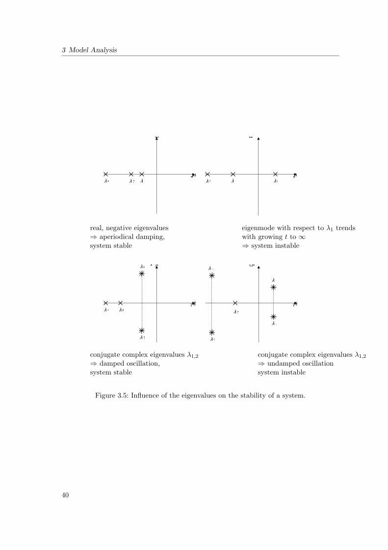
Figure 3.5 shows a graphical representation of these criteria.
The solution of x = Ax takes the form of a linear combination
x(t) =n∑
i=1
eλitci . (3.64)
The values of the ci depend on the initial conditions x(0) = x0. The addends eλitci arealso called the eigenmodes of the system.
Example
Consider the differential equation system
x = Ax =
1 0 −10 1 −10 1 1
x , (3.65)
x(0) = [1, 2, 0]T . (3.66)
In Section 3.7 we have calculated the eigenvalues
λ1 = 1 , λ2 = 1 + i , λ3 = 1− i . (3.67)
As there is at least one eigenvalue with a positive real part – in fact all real parts arepositive – the system is unstable. Furthermore, the system shows an oscillation withfrequency 2π.
Although this is rarely done in practice, we apply the coordinate transformation describedabove for illustrative purposes. The matrix Λ of the eigenvalues is
Λ =
λ1 0 00 Re(λ2) − Im(λ2)0 Im(λ2) Re(λ2)
=
1 0 00 1 −10 1 1
, (3.68)
39
3 Model Analysis
λ λλ λ λ λ
real, negative eigenvalues eigenmode with respect to λ1 trends⇒ aperiodical damping, with growing t to ∞system stable ⇒ system instable
λ λλ
λ
λ
λ
λ
λ
λ
conjugate complex eigenvalues λ1,2 conjugate complex eigenvalues λ1,2
⇒ damped oscillation, ⇒ undamped oscillationsystem stable system instable
Figure 3.5: Influence of the eigenvalues on the stability of a system.
40
3.8 Stability
and for2
T =
1 1 00 1 00 0 1
, T−1 =
1 −1 00 1 00 0 1
, (3.69)
we have Λ = T−1AT . If we define
z = T−1x , (3.70)
then equation (3.65) becomes
z = Λz , (3.71)
z(0) = T−1x(0) = [−1, 2, 0]T . (3.72)
The solution in terms of z is
z1(t) = −et , (3.73)
z2(t) = c1e(1+i)t + c2e
(1−i)t , (3.74)
z3(t) = c3e(1+i)t + c4e
(1−i)t . (3.75)
The coefficients ci are 3
c1 = 1 , c2 = 1 , (3.76)c3 = −i c4 = i , (3.77)
and thus
z1(t) = −et , (3.78)
z2(t) = e(1+i)t + e(1−i)t = 2et cos t , (3.79)
z3(t) = −ie(1+i)t + ie(1−i)t = 2et sin t ; (3.80)
for the latter transformation, we have used Euler’s formula eiφ = cos φ + i sin φ. Finally,we get the solution for x = Tz:
x1(t) = z1(t) + z2(t) = et(−1 + 2 cos t) , (3.81)x2(t) = z2(t) = 2et cos t , (3.82)x3(t) = z3(t) = 2et sin t . (3.83)
2The calculation of a matrix T fulfilling the given condition is not the subject of this course.3The calculation of the coefficients ci is left as an exercise to the reader. Hint: Solve the linear equation
system for c1,... , c4 that consists of the initial conditions for z2 and z3 as well as two further equationsresulting from the differential equations z2 = z2 − z3 and z3 = z2 + z3.
41
3 Model Analysis
3.9 Time Characteristics
The time characteristics of a linearized system can be determined by means of its eigen-values:
For real eigenvalues λreali ∈ R, the time constants
T time constanti =
1|λreal
i |(3.84)
are a measure for the increase or decrease of the corresponding eigenmode eλreali tci.
For pairs of imaginary eigenvalues λimag±i = ±bii ∈ Ri,
T oscillationi =
2π
|λimag±|=
2π
|bi|(3.85)
is the oscillation period of the eigenmode eλimag±i tci = [ cos(bit)± i sin(bit) ]ci.
For complex eigenvalues λcom±i = ai ± bii ∈ C with ai, bi 6= 0, the corresponding
eigenmodes show damped or excited oscillations (depending on the sign of ai) withthe time constant
T time constanti =
1|Re(λcom±
i )|=
1|ai|
(3.86)
and the oscillation period
T oscillationi =
2π
| Im(λcom±i )|
=2π
|bi|. (3.87)
The minimal and the maximal time characteristic of the entire system are
Tmin = min(T time constanti , T oscillation
i ) (3.88)
and
Tmax = max(T time constanti , T oscillation
i ) (3.89)
As already introduced, you choose as simulation time tsim = 5·Tmax, if the system is stable.Otherwise, tsim depends on an upper limit M : |x(t)| ≤ M or the problem formulation.
You choose the time step length h = ∆t ≤ α · Tmin with the time step index α =h
Tmin∈[
120
,15
], leading to (5 . . . 20) · h = Tmin.
42
3.10 Problem: Stiff Differential Equations
Example
For the example in Section 3.8, we have found the real eigenvalue λ1 = 1 with
T time constant1 =
1|1|
= 1 (3.90)
and the complex eigenvalues λ2,3 = 1± i with
T time constant2,3 =
1|1|
= 1 , (3.91)
T oscillation2,3 =
2π
|i|= 2π . (3.92)
The maximal time characteristic of the system is 2π, and its minimal time characteristicis 1.
3.10 Problem: Stiff Differential Equations
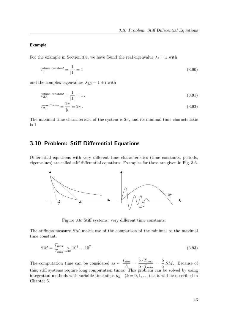
Differential equations with very different time characteristics (time constants, periods,eigenvalues) are called stiff differential equations. Examples for these are given in Fig. 3.6.
ω
ω
Figure 3.6: Stiff systems: very different time constants.
The stiffness measure SM makes use of the comparison of the minimal to the maximaltime constant:
SM =Tmax
Tmin>stiff
103 . . . 107 (3.93)
The computation time can be considered as ∼ tsimh
=5 · Tmax
α · Tmin=
5α
SM . Because of
this, stiff systems require long computation times. This problem can be solved by usingintegration methods with variable time steps hk (k = 0, 1, . . . ) as it will be described inChapter 5.
43
3 Model Analysis
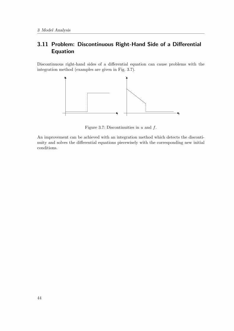
3.11 Problem: Discontinuous Right-Hand Side of a DifferentialEquation
Discontinuous right-hand sides of a differential equation can cause problems with theintegration method (examples are given in Fig. 3.7).
Figure 3.7: Discontinuities in u and f .
An improvement can be achieved with an integration method which detects the disconti-nuity and solves the differential equations piecewisely with the corresponding new initialconditions.
44
4 Basic Numerical Concepts
In this chapter, a few basic concepts of numerical mathematics, which are of interestfor the simulation techniques, will be reviewed very briefly. For detailed presentationsthe well-known fundamental books (e.g. Press et al. (1990), Engeln-Muller and Reutter(1993)) and lecture notes (e.g. Dahmen (1994)) are recommended. The requirements onnumerical methods can be summarized in these key words:
robustness (the solution should be found),
reliability (high accuracy), and
efficiency (short computation time).
This chapter deals with major issues regarding possible numerical errors and their effects.Generally, you can distinguish the following kinds of errors:
model errors,
data errors,
rounding errors, and
method errors.
4.1 Floating Point Numbers
Numbers are saved in computers as floating point numbers in the normalized floatingpoint representation. A well-known example for this representation of real numbers is thescientific notation:
12 = 1.20E1 = 1.20 · 101, 0.375 = 3.75E -1 = 3.75 · 10−1. (4.1)
In these examples, number are represented in the form f · 10e, where f is a three-digitnumber with 1 ≤ f < 10. The exponent e is an integer. This notation can be generalizedin several respects. For a particular floating point representation, we have to choose:
a base b ∈ N, b ≥ 2,
45
4 Basic Numerical Concepts
a minimum exponent r ∈ Z and a maximum exponent R ∈ Z with r ≤ R,
and the number of digits for the representation of a number, d ∈ N.
For instance, if we choose b = 10, r = −5, R = 5, and d = 3, the examples in equation(4.1) are valid floating point numbers. In general, a floating point number x can be written
x = f · be, (4.2)
where the mantissa f is a number with d digits, 1 ≤ f < b, and the exponent e is an integerwith r ≤ e ≤ R. If we choose the base b = 2, then we get the following representations forthe examples above:
12 = 1 · 23 + 1 · 22 0.375 = 1 · 2−2 + 1 · 2−3
= (1 · 20 + 1 · 2−1) · 23 = (1 · 20 + 1 · 2−1) · 2−2
= 1.1Á · 211Á , = 1.1Á · 2−10Á .
Binary numbers are marked with Á. In a binary representation, only the two digits “0”and “1” are needed. Therefore, binary numbers are very well suited for the representationof numbers in computers: The two digits can be mapped to the two states “voltage” and“no voltage” in an electrical circuit. As the reader is assumed to be much more familiarwith decimal numbers, we will use b = 10 in the following discussion. Note that all remarksare in principle valid for any choice of the base b.
4.2 Rounding Errors
For any choice of b, d, r, and R, the set A of the floating point numbers f ·be is finite. Dueto this limitation, not all real numbers x ∈ R can be written in floating point notation.For instance, for x = 1
3 , we have (b = 10, d = 3)
3.33 · 10−1 <13
< 3.34 · 10−1. (4.3)
Therefore, we introduce a rounding function rd : R → A that maps a real number x tothe “nearest” floating point number; i.e. for any x ∈ R, this rounding function fulfils thecondition
|x− rd(x)︸ ︷︷ ︸machine number
| ≤ |x− g| for all g ∈ A. (4.4)
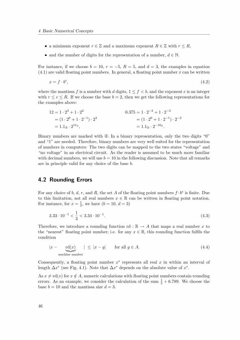
Consequently, a floating point number x∗ represents all real x in within an interval oflength ∆x∗ (see Fig. 4.1). Note that ∆x∗ depends on the absolute value of x∗.
As x 6= rd(x) for x /∈ A, numeric calculations with floating point numbers contain roundingerrors. As an example, we consider the calculation of the sum 1
3 + 6.789. We choose thebase b = 10 and the mantissa size d = 3.
46
4.2 Rounding Errors
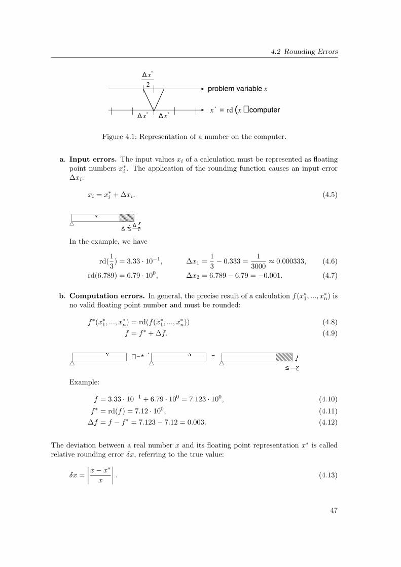
( )=∗∗∆ ∗∆
∗∆
Figure 4.1: Representation of a number on the computer.
a. Input errors. The input values xi of a calculation must be represented as floatingpoint numbers x∗i . The application of the rounding function causes an input error∆xi:
xi = x∗i + ∆xi. (4.5)
∗∆≤∆
∗
In the example, we have
rd(13) = 3.33 · 10−1, ∆x1 =
13− 0.333 =
13000
≈ 0.000333, (4.6)
rd(6.789) = 6.79 · 100, ∆x2 = 6.789− 6.79 = −0.001. (4.7)
b. Computation errors. In general, the precise result of a calculation f(x∗1, ..., x∗n) is
no valid floating point number and must be rounded:
f∗(x∗1, ..., x∗n) = rd(f(x∗1, ..., x
∗n)) (4.8)
f = f∗ + ∆f. (4.9)
∗
≤
=∗−+
Example:
f = 3.33 · 10−1 + 6.79 · 100 = 7.123 · 100, (4.10)
f∗ = rd(f) = 7.12 · 100, (4.11)∆f = f − f∗ = 7.123− 7.12 = 0.003. (4.12)
The deviation between a real number x and its floating point representation x∗ is calledrelative rounding error δx, referring to the true value:
δx =∣∣∣∣x− x∗
x
∣∣∣∣ . (4.13)
47
4 Basic Numerical Concepts
The machine accuracy ε (resolution of the computer) is an upper limit for the relativerounding error:
δx ≤ ε for all x. (4.14)
For an ordinary PC, this value is 10−16.
As an example for effects of rounding errors, we will study the calculation of the cosinefunction. Its series expansion is the following:
cos x =∞∑
k=0
cos(k)(0)k!
xk =cos 00!
x0 − sin 01!
x1 − cos 02!
x2 +sin 03!
x3 + . . .
= 1− x2
2!+
x4
4!− x6
6!+ . . .
=∞∑
k=0
(−1)k x2k
(2k)!. (4.15)
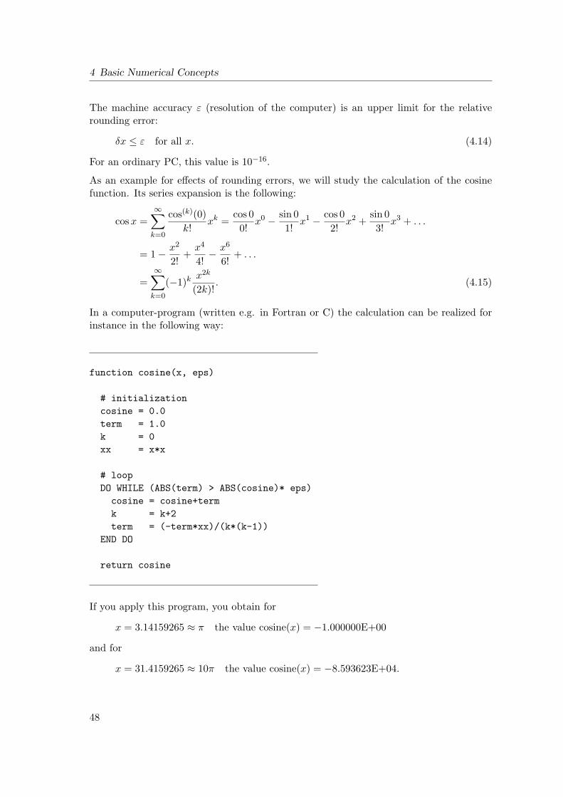
In a computer-program (written e.g. in Fortran or C) the calculation can be realized forinstance in the following way:
function cosine(x, eps)
# initializationcosine = 0.0term = 1.0k = 0xx = x*x
# loopDO WHILE (ABS(term) > ABS(cosine)* eps)
cosine = cosine+termk = k+2term = (-term*xx)/(k*(k-1))
END DO
return cosine
If you apply this program, you obtain for
x = 3.14159265 ≈ π the value cosine(x) = −1.000000E+00
and for
x = 31.4159265 ≈ 10π the value cosine(x) = −8.593623E+04.
48
4.3 Conditioning
The cause for this effect are so-called cancellation errors:
30th sum term: term30 = −3.0962506 · 1012,
60th sum term: term60 = −8.1062036 · 107.
Because the size of the mantissa is limited to d = 7, you obtain:
term30 = −3.0962506E+12+ term60 = −0.0000811E+12 (from the third digit on all numerals get lost)
−3.0963317E+12
The solution of the series expansion depends on the summation order. Therefore, it issensible to change the summation order and to calculate the small terms first.
4.3 Conditioning
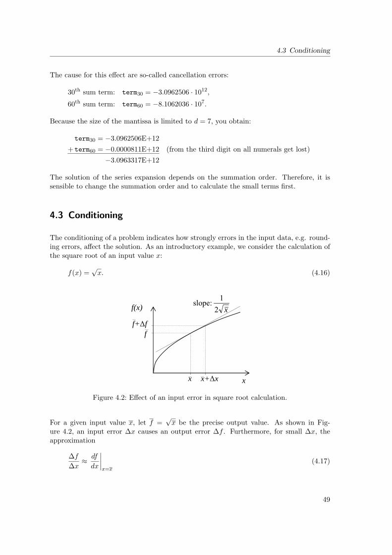
The conditioning of a problem indicates how strongly errors in the input data, e.g. round-ing errors, affect the solution. As an introductory example, we consider the calculation ofthe square root of an input value x:
f(x) =√
x. (4.16)
x
f(x)
x+∆xx
f+∆ff
slope:x21
Figure 4.2: Effect of an input error in square root calculation.
For a given input value x, let f =√
x be the precise output value. As shown in Fig-ure 4.2, an input error ∆x causes an output error ∆f . Furthermore, for small ∆x, theapproximation
∆f
∆x≈ df
dx
∣∣∣∣x=x
(4.17)
49
4 Basic Numerical Concepts
is valid, hence
∆f ≈ ∆xdf
dx
∣∣∣∣x=x
=∆x
2√
x(4.18)
For the relative errors δx and δf , we get the relation
δf =∆f
f≈
(∆x2√
x
)√
x=
12· ∆x
x=
12δx. (4.19)
In general, an output value f can depend on n input values xj . Consequently, an errorin each of the input values affects the output. This influence can be calculated using aTaylor expansion of f which is truncated after the first-order term:
f(x + ∆x) = f(x) +n∑
j=1
∂f
∂xj
∣∣∣∣x=x
∆xj + . . . . (4.20)
For the relative error δf , we obtain under the conditions f(x) 6= 0 and ∀j ∈ 1, . . . , n :xj 6= 0 the expression
δf =f(x + ∆x)− f(x)
f(x)=
n∑j=1
∂f
∂xj
∣∣∣∣x=x
xj
f(x)︸ ︷︷ ︸Kj
· ∆xj
xj︸︷︷︸δxj
, (4.21)
δf =n∑
j=1
Kjδxj . (4.22)
The relative error δxj of each input value contributes to the relative output error. Theamplification factor or relative condition number Kj is a measure for the contribution ofan error in the corresponding input value. Hence, a problem is ill-conditioned with respectto an input xj if |Kj | is big (> 1). The smaller the absolute values of the amplificationfactors are, the better the conditioning of the problem is.
We have already determined the amplification factor for the calculation of the square root(equation (4.19)):
δ√x =12δx, K =
12. (4.23)
For the multiplication, we get:
f(x1, x2) = x1x2, (4.24)
K1 =∂f
∂x1
∣∣∣∣x1,x2
x1
f(x1, x2)= x2 ·
x1
x1x2= 1 for x1, x2 6= 0, (4.25)
and, by analogy, K2 = 1. The conditioning of the arithmetic operations is given inTable. 4.1.
50
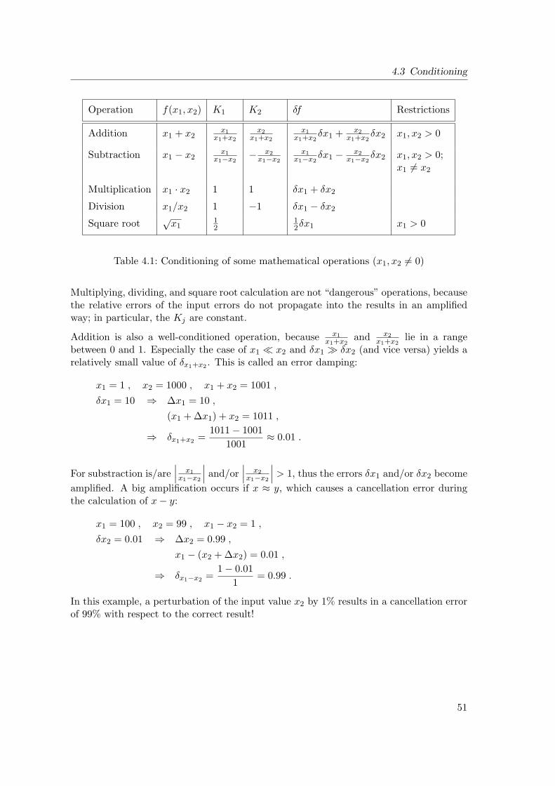
4.3 Conditioning
Operation f(x1, x2) K1 K2 δf Restrictions
Addition x1 + x2x1
x1+x2
x2x1+x2
x1x1+x2
δx1 + x2x1+x2
δx2 x1, x2 > 0
Subtraction x1 − x2x1
x1−x2− x2
x1−x2
x1x1−x2
δx1 − x2x1−x2
δx2 x1, x2 > 0;x1 6= x2
Multiplication x1 · x2 1 1 δx1 + δx2
Division x1/x2 1 −1 δx1 − δx2
Square root√
x112
12δx1 x1 > 0
Table 4.1: Conditioning of some mathematical operations (x1, x2 6= 0)
Multiplying, dividing, and square root calculation are not “dangerous” operations, becausethe relative errors of the input errors do not propagate into the results in an amplifiedway; in particular, the Kj are constant.
Addition is also a well-conditioned operation, because x1x1+x2
and x2x1+x2
lie in a rangebetween 0 and 1. Especially the case of x1 x2 and δx1 δx2 (and vice versa) yields arelatively small value of δx1+x2 . This is called an error damping:
x1 = 1 , x2 = 1000 , x1 + x2 = 1001 ,
δx1 = 10 ⇒ ∆x1 = 10 ,
(x1 + ∆x1) + x2 = 1011 ,
⇒ δx1+x2 =1011− 1001
1001≈ 0.01 .
For substraction is/are∣∣∣ x1x1−x2
∣∣∣ and/or∣∣∣ x2x1−x2
∣∣∣ > 1, thus the errors δx1 and/or δx2 becomeamplified. A big amplification occurs if x ≈ y, which causes a cancellation error duringthe calculation of x− y:
x1 = 100 , x2 = 99 , x1 − x2 = 1 ,
δx2 = 0.01 ⇒ ∆x2 = 0.99 ,
x1 − (x2 + ∆x2) = 0.01 ,
⇒ δx1−x2 =1− 0.01
1= 0.99 .
In this example, a perturbation of the input value x2 by 1% results in a cancellation errorof 99% with respect to the correct result!
51

4 Basic Numerical Concepts
52
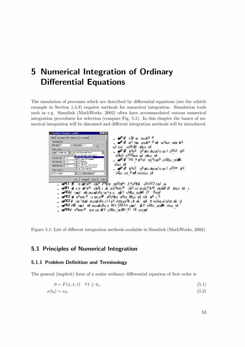
5 Numerical Integration of OrdinaryDifferential Equations
The simulation of processes which are described by differential equations (see the vehicleexample in Section 1.3.3) requires methods for numerical integration. Simulation toolssuch as e.g. Simulink (MathWorks, 2002) often have accommodated various numericalintegration procedures for selection (compare Fig. 5.1). In this chapter the basics of nu-merical integration will be discussed and different integration methods will be introduced.
! "# $ % &' () * +, -. / 01 2 34 56 7 89 : ;<
=> ?@A B C D EF GH I JK LM N OPRQS T UV W XY Z [\ ]^`_ a bdc e fhg ij klm no pq rs tu vwyx z |
~ R y ¡ ¢£ ¤¥ ¦ § ¨ ©ª «¬ ® ¯ °± ²³ ´¶µ ·¸ ¹ºh»
¼½ ¾¿ À ÁÂRÃÄ Å ÆÇ È ÉÊ Ë ÌÍ ÎÏ`Ð Ñ ÒdÓ Ô ÕhÖ ×Ø ÙÚÛ ÜÝ Þß àá âã äåyæ ç èé
êë ìí îï ðdñ òó ôõ ö÷ øù úû ü ýþRÿ
"! #$ % &'( ) * +-, ./ 0 1243 5 67 89 :; <>= ?@BAC D EF GH I JK LM NO PQ RST UV WX YZ [ \>] ^_ `a bc de f g hi jk lm n op q rs tuv wx yz | ~ B 4 ¡ ¢£ ¤¥ ¦§ ¨ © ª «¬ ® ¯>° ±² ³"´ µ>¶ ·¸4¹ º»½¼ ¾ ¿ ÀÁ ÂÃBÄÅ Æ ÇÈ ÉÊ Ë ÌÍ ÎÏ ÐÑ ÒÓ Ô Õ Ö× Ø ÙÚÛ Ü Ý Þß àá â ãä åæ ç èé êë ì íî ï ðñ ò óô õ ö½÷ø ù úû üý þ ÿ ! " #$ % &' ( ) *+ , - . /0 12 3 45 67 89 : ;< = >@?A B CED FG H I JK LM NO P QR ST U VW X YZ [\ ] ^_ ` ab cdfe gh ij k l mn op qsr tu vxw ysz | ~ E s¡ ¢£ ¤x¥ ¦s§ ¨©ª «¬f ® ¯° ±² ³´ µ¶·
Figure 5.1: List of different integration methods available in Simulink (MathWorks, 2002).
5.1 Principles of Numerical Integration
5.1.1 Problem Definition and Terminology
The general (implicit) form of a scalar ordinary differential equation of first order is
0 = F (x, x, t) ∀ t ≥ t0 , (5.1)x(t0) = x0 . (5.2)
53
5 Numerical Integration of Ordinary Differential Equations
Example
0 = 2x + x ∀ t ≥ 0 , (5.3)x(0) = 1 . (5.4)
Note that in this example, there is no explicit dependency of F on t.
We will restrict our presentation to differential equations that are given in the explicitform
x = f(x, t) ∀ t ≥ t0 , (5.5)x(t0) = x0 . (5.6)
Sometimes, it is possible to transform a DE in implicit form into the explicit form.
Example
The example above can easily be transformed into
x = −x
2∀ t ≥ 0 , (5.7)
x(0) = 1 . (5.8)
Solving a differential equation (DE) means to find a function x : R → R such that thedifferential equation (5.1) as well as the initial condition (5.2) are fulfilled. We will denotethis exact solution as x(t). In Section 3.2 we have discussed a sufficient criterion for theexistence of a unique solution.
In general, x(t) cannot be calculated analytically. Rather, we must apply a numericalintegration method in order to get an approximation of x(t). More precisely, a numericalmethod yields a set of N pairs (tk, xk) such that
xk ≈ x(tk) (5.9)
for all k. Each tk represents a discrete time point, and therefore the set tk|k = 1, ..., Nis called a discrete time grid. The time step length between tk and tk+1 is denoted hk, i.e.
tk+1 = tk + hk . (5.10)
To simplify the following discussion, we will assume a constant time step length h = hk,k = 1, ..., N such that we get an equidistant time grid.
54
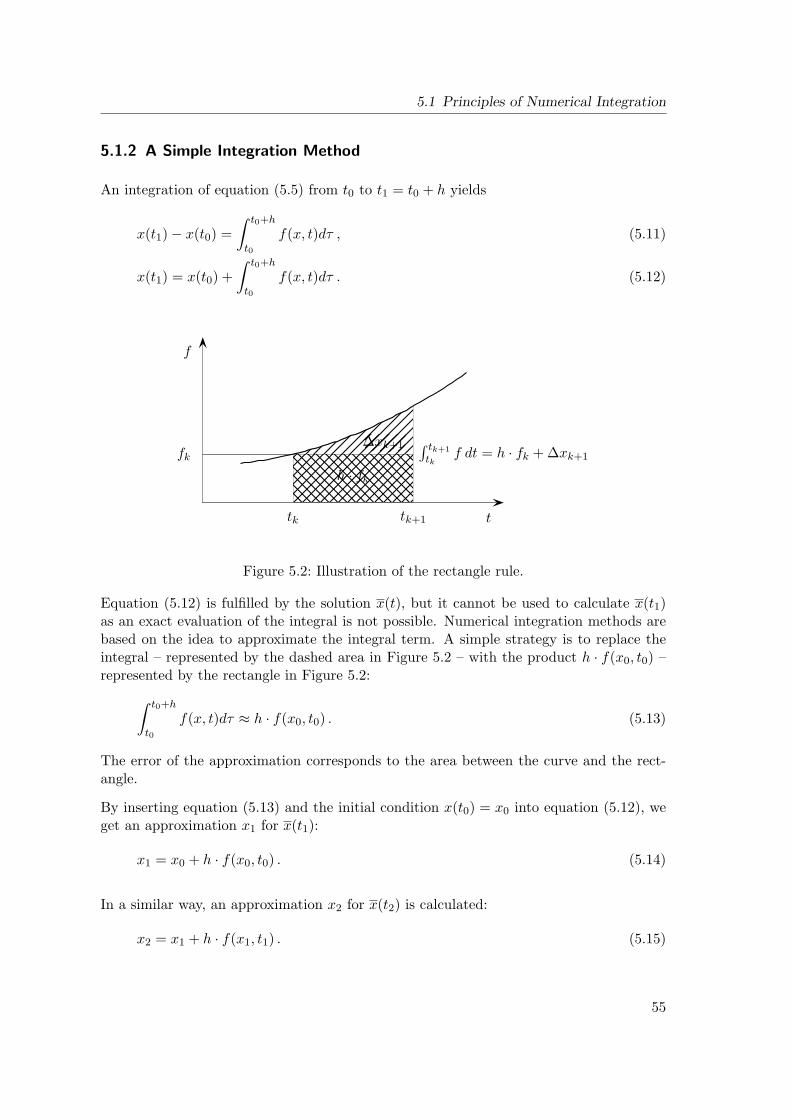
5.1 Principles of Numerical Integration
5.1.2 A Simple Integration Method
An integration of equation (5.5) from t0 to t1 = t0 + h yields
x(t1)− x(t0) =∫ t0+h
t0
f(x, t)dτ , (5.11)
x(t1) = x(t0) +∫ t0+h
t0
f(x, t)dτ . (5.12)
t
f
fk
tk tk+1
∫ tk+1
tkf dt = h · fk + ∆xk+1
h · fk
∆xk+1
Figure 5.2: Illustration of the rectangle rule.
Equation (5.12) is fulfilled by the solution x(t), but it cannot be used to calculate x(t1)as an exact evaluation of the integral is not possible. Numerical integration methods arebased on the idea to approximate the integral term. A simple strategy is to replace theintegral – represented by the dashed area in Figure 5.2 – with the product h · f(x0, t0) –represented by the rectangle in Figure 5.2:∫ t0+h
t0
f(x, t)dτ ≈ h · f(x0, t0) . (5.13)
The error of the approximation corresponds to the area between the curve and the rect-angle.
By inserting equation (5.13) and the initial condition x(t0) = x0 into equation (5.12), weget an approximation x1 for x(t1):
x1 = x0 + h · f(x0, t0) . (5.14)
In a similar way, an approximation x2 for x(t2) is calculated:
x2 = x1 + h · f(x1, t1) . (5.15)
55
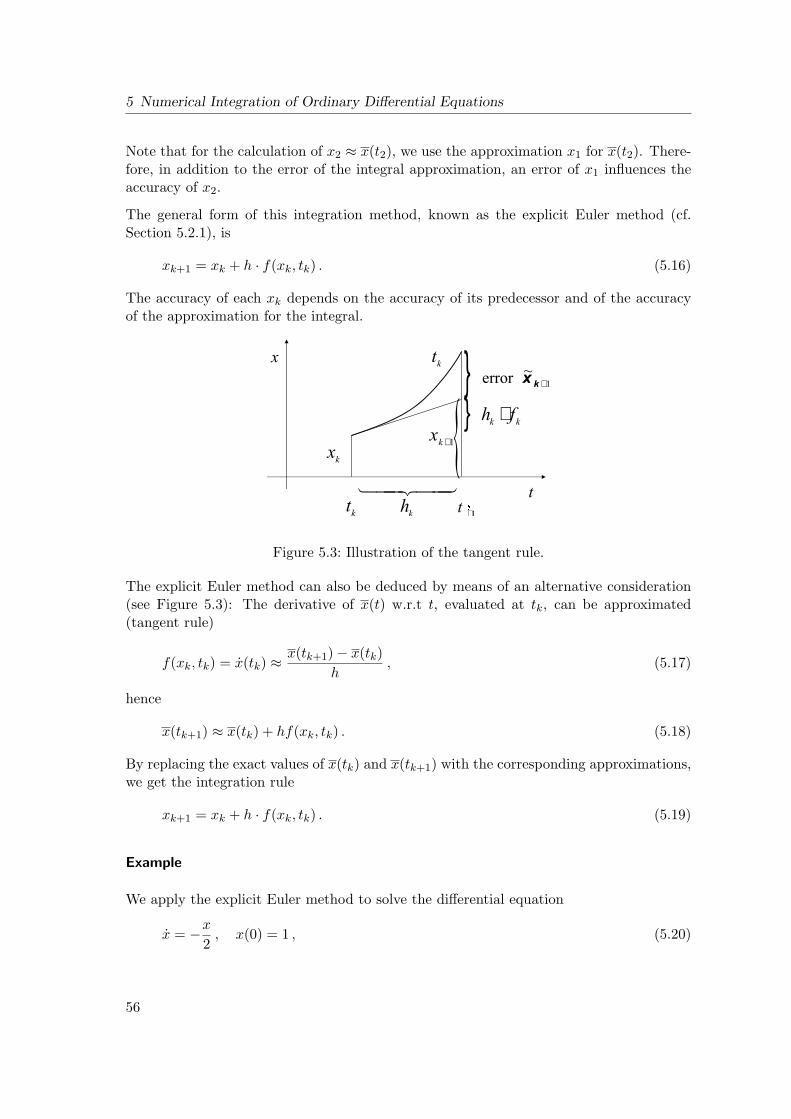
5 Numerical Integration of Ordinary Differential Equations
Note that for the calculation of x2 ≈ x(t2), we use the approximation x1 for x(t2). There-fore, in addition to the error of the integral approximation, an error of x1 influences theaccuracy of x2.
The general form of this integration method, known as the explicit Euler method (cf.Section 5.2.1), is
xk+1 = xk + h · f(xk, tk) . (5.16)
The accuracy of each xk depends on the accuracy of its predecessor and of the accuracyof the approximation for the integral.
+
⋅
+
+
Figure 5.3: Illustration of the tangent rule.
The explicit Euler method can also be deduced by means of an alternative consideration(see Figure 5.3): The derivative of x(t) w.r.t t, evaluated at tk, can be approximated(tangent rule)
f(xk, tk) = x(tk) ≈x(tk+1)− x(tk)
h, (5.17)
hence
x(tk+1) ≈ x(tk) + hf(xk, tk) . (5.18)
By replacing the exact values of x(tk) and x(tk+1) with the corresponding approximations,we get the integration rule
xk+1 = xk + h · f(xk, tk) . (5.19)
Example
We apply the explicit Euler method to solve the differential equation
x = −x
2, x(0) = 1 , (5.20)
56
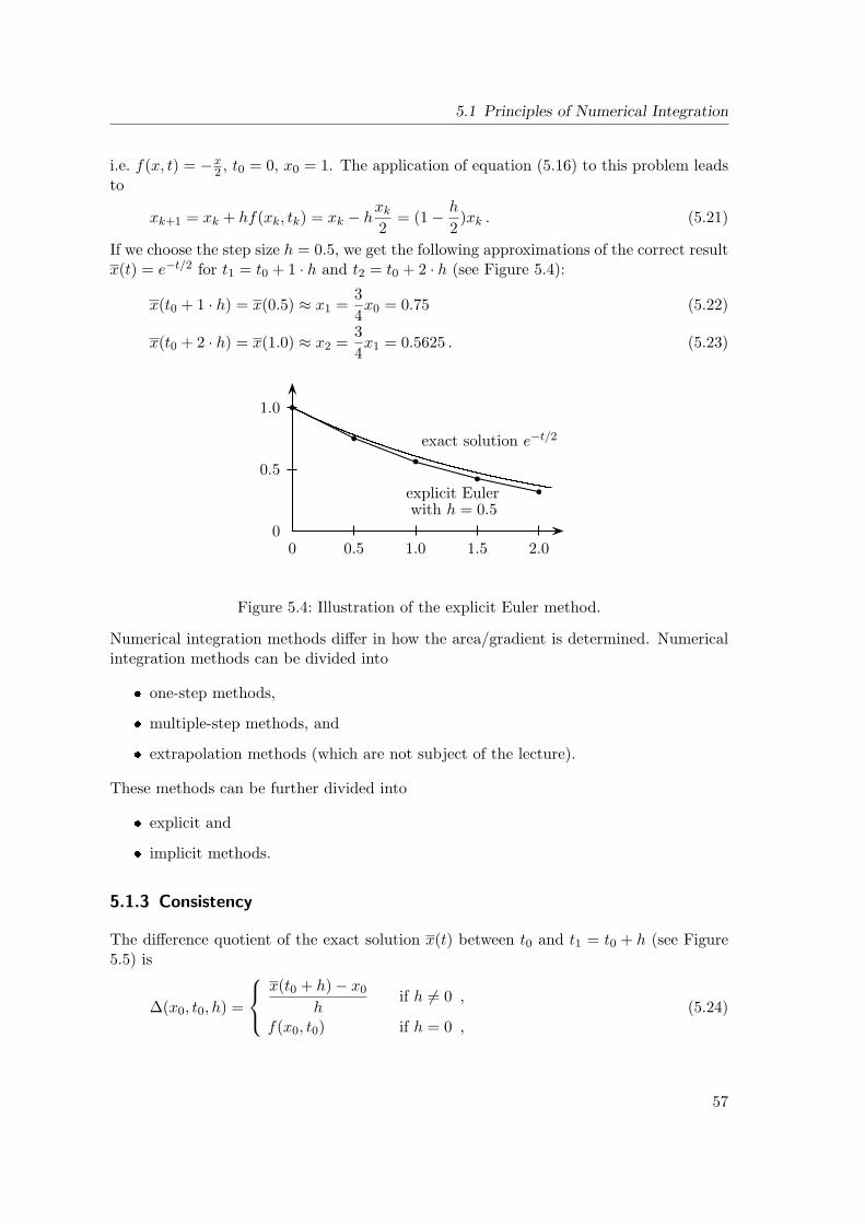
5.1 Principles of Numerical Integration
i.e. f(x, t) = −x2 , t0 = 0, x0 = 1. The application of equation (5.16) to this problem leads
to
xk+1 = xk + hf(xk, tk) = xk − hxk
2= (1− h
2)xk . (5.21)
If we choose the step size h = 0.5, we get the following approximations of the correct resultx(t) = e−t/2 for t1 = t0 + 1 · h and t2 = t0 + 2 · h (see Figure 5.4):
x(t0 + 1 · h) = x(0.5) ≈ x1 =34x0 = 0.75 (5.22)
x(t0 + 2 · h) = x(1.0) ≈ x2 =34x1 = 0.5625 . (5.23)
0 0.5 1.0 1.5 2.00
0.5
1.0 b
b
b
b
b
exact solution e−t/2
explicit Eulerwith h = 0.5
Figure 5.4: Illustration of the explicit Euler method.
Numerical integration methods differ in how the area/gradient is determined. Numericalintegration methods can be divided into
one-step methods,
multiple-step methods, and
extrapolation methods (which are not subject of the lecture).
These methods can be further divided into
explicit and
implicit methods.
5.1.3 Consistency
The difference quotient of the exact solution x(t) between t0 and t1 = t0 + h (see Figure5.5) is
∆(x0, t0, h) =
x(t0 + h)− x0
hif h 6= 0 ,
f(x0, t0) if h = 0 ,(5.24)
57
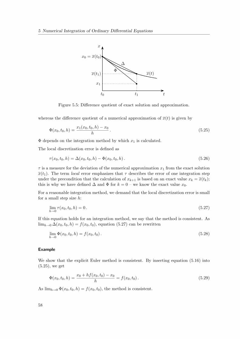
5 Numerical Integration of Ordinary Differential Equations
t0 t
x0 = x(t0)
x1
x(t1)
x
t1
x(t)b
b
b
∆
Φ
Figure 5.5: Difference quotient of exact solution and approximation.
whereas the difference quotient of a numerical approximation of x(t) is given by
Φ(x0, t0, h) =x1(x0, t0, h)− x0
h. (5.25)
Φ depends on the integration method by which x1 is calculated.
The local discretization error is defined as
τ(x0, t0, h) = ∆(x0, t0, h)− Φ(x0, t0, h) . (5.26)
τ is a measure for the deviation of the numerical approximation x1 from the exact solutionx(t1). The term local error emphasizes that τ describes the error of one integration stepunder the precondition that the calculation of xk+1 is based on an exact value xk = x(tk);this is why we have defined ∆ and Φ for k = 0 – we know the exact value x0.
For a reasonable integration method, we demand that the local discretization error is smallfor a small step size h:
limh→0
τ(x0, t0, h) = 0 . (5.27)
If this equation holds for an integration method, we say that the method is consistent. Aslimh→0 ∆(x0, t0, h) = f(x0, t0), equation (5.27) can be rewritten
limh→0
Φ(x0, t0, h) = f(x0, t0) . (5.28)
Example
We show that the explicit Euler method is consistent. By inserting equation (5.16) into(5.25), we get
Φ(x0, t0, h) =x0 + hf(x0, t0)− x0
h= f(x0, t0) . (5.29)
As limh→0 Φ(x0, t0, h) = f(x0, t0), the method is consistent.
58
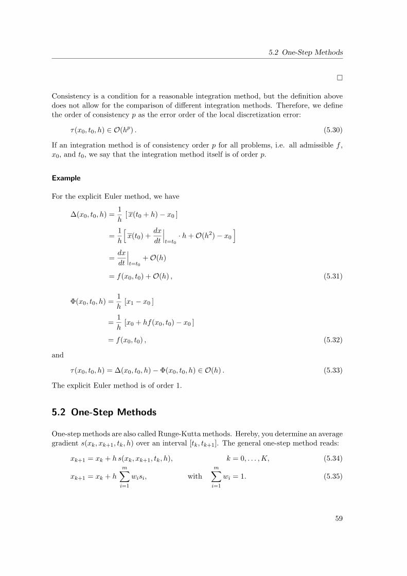
5.2 One-Step Methods
Consistency is a condition for a reasonable integration method, but the definition abovedoes not allow for the comparison of different integration methods. Therefore, we definethe order of consistency p as the error order of the local discretization error:
τ(x0, t0, h) ∈ O(hp) . (5.30)
If an integration method is of consistency order p for all problems, i.e. all admissible f ,x0, and t0, we say that the integration method itself is of order p.
Example
For the explicit Euler method, we have
∆(x0, t0, h) =1h
[x(t0 + h)− x0 ]
=1h
[x(t0) +
dx
dt
∣∣∣t=t0
· h +O(h2)− x0
]=
dx
dt
∣∣∣t=t0
+O(h)
= f(x0, t0) +O(h) , (5.31)
Φ(x0, t0, h) =1h
[x1 − x0 ]
=1h
[x0 + hf(x0, t0)− x0 ]
= f(x0, t0) , (5.32)
and
τ(x0, t0, h) = ∆(x0, t0, h)− Φ(x0, t0, h) ∈ O(h) . (5.33)
The explicit Euler method is of order 1.
5.2 One-Step Methods
One-step methods are also called Runge-Kutta methods. Hereby, you determine an averagegradient s(xk, xk+1, tk, h) over an interval [tk, tk+1]. The general one-step method reads:
xk+1 = xk + h s(xk, xk+1, tk, h), k = 0, . . . ,K, (5.34)
xk+1 = xk + h
m∑i=1
wisi, withm∑
i=1
wi = 1. (5.35)
59
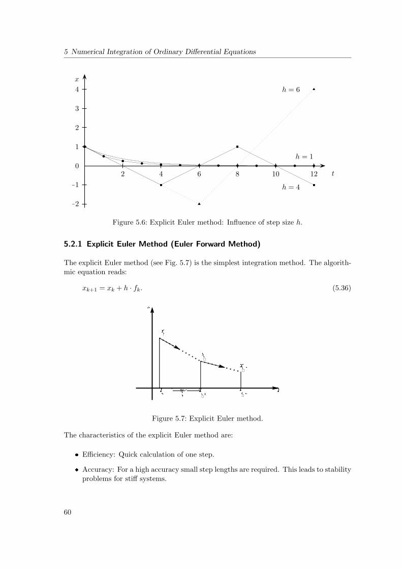
5 Numerical Integration of Ordinary Differential Equations
2 4 6 8 10 120
1
2
3
4
−1
−2
b
b
bb
b b b b b b b b b
r
r
r
r
u
u
u
t
x
h = 1
h = 4
h = 6
Figure 5.6: Explicit Euler method: Influence of step size h.
5.2.1 Explicit Euler Method (Euler Forward Method)
The explicit Euler method (see Fig. 5.7) is the simplest integration method. The algorith-mic equation reads:
xk+1 = xk + h · fk. (5.36)
+
+
+
+
Figure 5.7: Explicit Euler method.
The characteristics of the explicit Euler method are:
Efficiency: Quick calculation of one step.
Accuracy: For a high accuracy small step lengths are required. This leads to stabilityproblems for stiff systems.
60
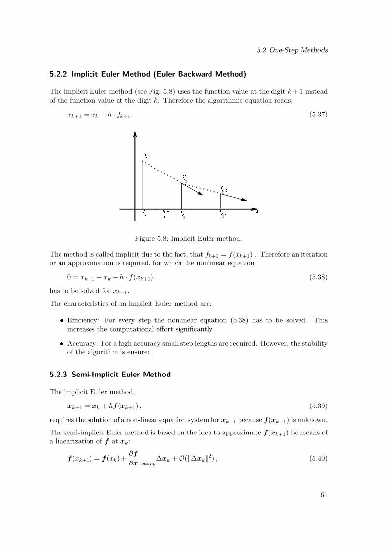
5.2 One-Step Methods
5.2.2 Implicit Euler Method (Euler Backward Method)
The implicit Euler method (see Fig. 5.8) uses the function value at the digit k + 1 insteadof the function value at the digit k. Therefore the algorithmic equation reads:
xk+1 = xk + h · fk+1. (5.37)
+
+
+
+
Figure 5.8: Implicit Euler method.
The method is called implicit due to the fact, that fk+1 = f(xk+1) . Therefore an iterationor an approximation is required, for which the nonlinear equation
0 = xk+1 − xk − h · f(xk+1). (5.38)
has to be solved for xk+1.
The characteristics of an implicit Euler method are:
Efficiency: For every step the nonlinear equation (5.38) has to be solved. Thisincreases the computational effort significantly.
Accuracy: For a high accuracy small step lengths are required. However, the stabilityof the algorithm is ensured.
5.2.3 Semi-Implicit Euler Method
The implicit Euler method,
xk+1 = xk + hf(xk+1) , (5.39)
requires the solution of a non-linear equation system for xk+1 because f(xk+1) is unknown.
The semi-implicit Euler method is based on the idea to approximate f(xk+1) be means ofa linearization of f at xk:
f(xk+1) = f(xk) +∂f
∂x
∣∣∣x=xk
∆xk +O(‖∆xk‖2) , (5.40)
61
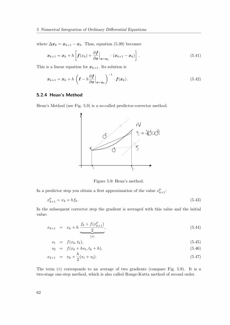
5 Numerical Integration of Ordinary Differential Equations
where ∆xk = xk+1 − xk. Thus, equation (5.39) becomes
xk+1 = xk + h
[f(xk) +
∂f
∂x
∣∣∣x=xk
· (xk+1 − xk)]
. (5.41)
This is a linear equation for xk+1. Its solution is
xk+1 = xk + h
(I − h
∂f
∂x
∣∣∣x=xk
)−1
· f(xk) . (5.42)
5.2.4 Heun’s Method
Heun’s Method (see Fig. 5.9) is a so-called predictor-corrector method.
+
+
( )
+=+
Figure 5.9: Heun’s method.
In a predictor step you obtain a first approximation of the value xpk+1:
xpk+1 = xk + hfk. (5.43)
In the subsequent corrector step the gradient is averaged with this value and the initialvalue:
xk+1 = xk + hfk + f(xp
k+1)2︸ ︷︷ ︸(∗)
, (5.44)
s1 = f(xk, tk), (5.45)s2 = f(xk + hs1, tk + h), (5.46)
xk+1 = xk +h
2(s1 + s2). (5.47)
The term (∗) corresponds to an average of two gradients (compare Fig. 5.9). It is atwo-stage one-step method, which is also called Runge-Kutta method of second order.
62
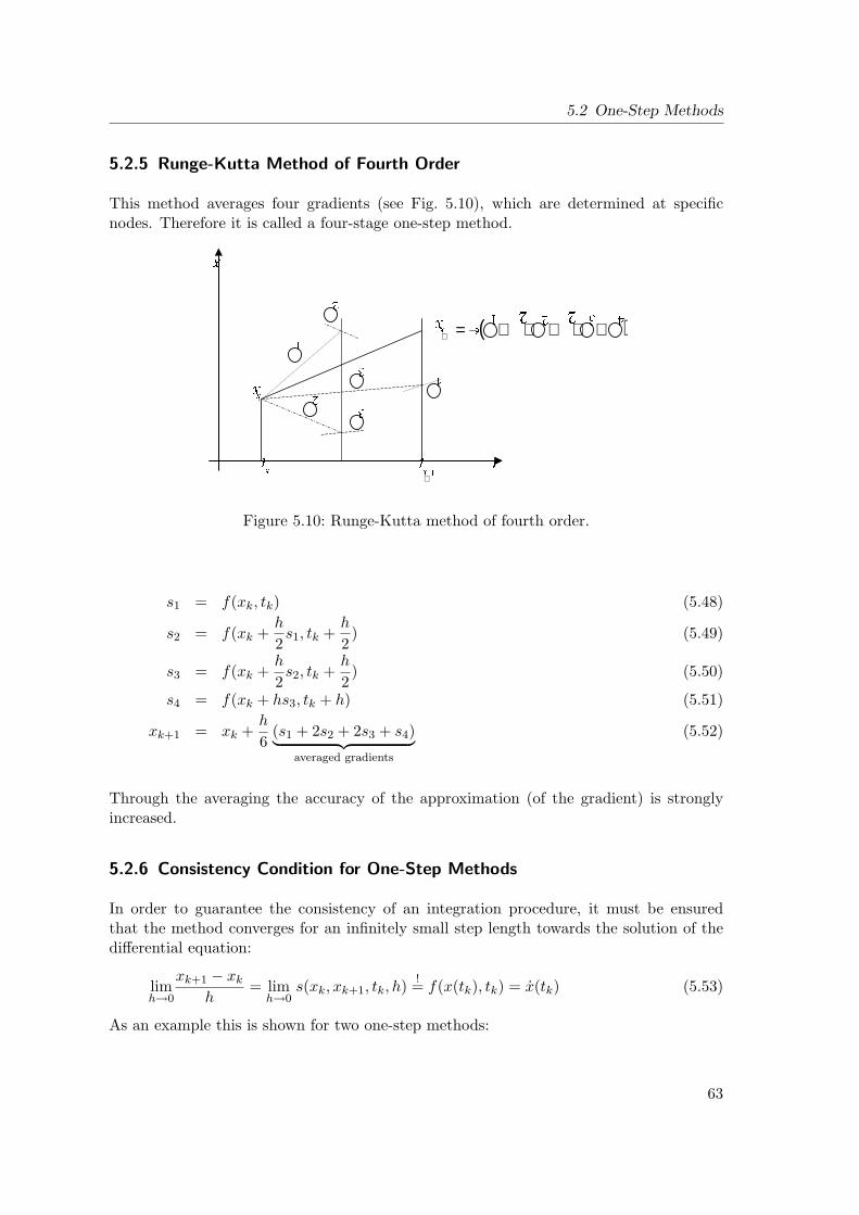
5.2 One-Step Methods
5.2.5 Runge-Kutta Method of Fourth Order
This method averages four gradients (see Fig. 5.10), which are determined at specificnodes. Therefore it is called a four-stage one-step method.
+
( )
+⋅+⋅+=+
Figure 5.10: Runge-Kutta method of fourth order.
s1 = f(xk, tk) (5.48)
s2 = f(xk +h
2s1, tk +
h
2) (5.49)
s3 = f(xk +h
2s2, tk +
h
2) (5.50)
s4 = f(xk + hs3, tk + h) (5.51)
xk+1 = xk +h
6(s1 + 2s2 + 2s3 + s4)︸ ︷︷ ︸
averaged gradients
(5.52)
Through the averaging the accuracy of the approximation (of the gradient) is stronglyincreased.
5.2.6 Consistency Condition for One-Step Methods
In order to guarantee the consistency of an integration procedure, it must be ensuredthat the method converges for an infinitely small step length towards the solution of thedifferential equation:
limh→0
xk+1 − xk
h= lim
h→0s(xk, xk+1, tk, h) != f(x(tk), tk) = x(tk) (5.53)
As an example this is shown for two one-step methods:
63
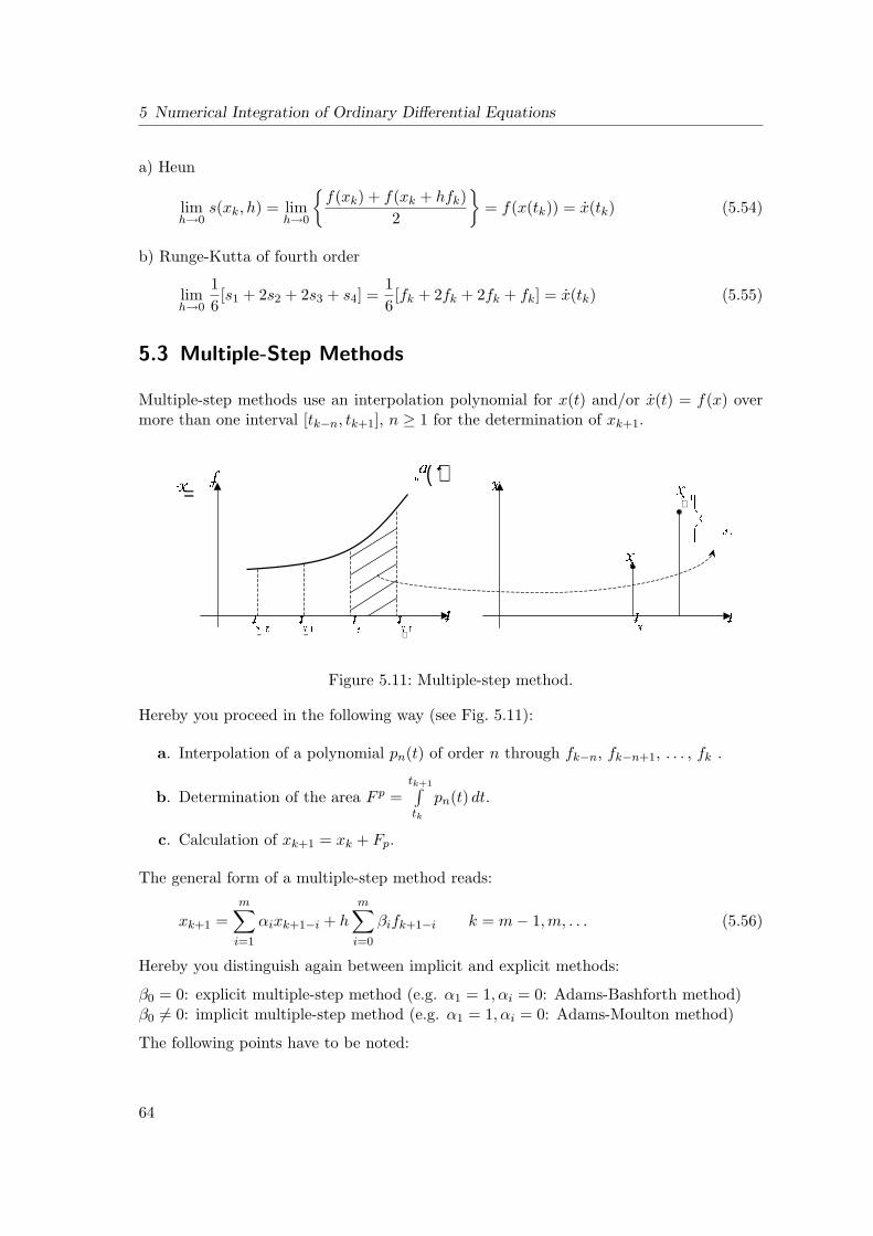
5 Numerical Integration of Ordinary Differential Equations
a) Heun
limh→0
s(xk, h) = limh→0
f(xk) + f(xk + hfk)
2
= f(x(tk)) = x(tk) (5.54)
b) Runge-Kutta of fourth order
limh→0
16[s1 + 2s2 + 2s3 + s4] =
16[fk + 2fk + 2fk + fk] = x(tk) (5.55)
5.3 Multiple-Step Methods
Multiple-step methods use an interpolation polynomial for x(t) and/or x(t) = f(x) overmore than one interval [tk−n, tk+1], n ≥ 1 for the determination of xk+1.
=
+
−
−
( )
+
Figure 5.11: Multiple-step method.
Hereby you proceed in the following way (see Fig. 5.11):
a. Interpolation of a polynomial pn(t) of order n through fk−n, fk−n+1, . . . , fk .
b. Determination of the area F p =tk+1∫tk
pn(t) dt.
c. Calculation of xk+1 = xk + Fp.
The general form of a multiple-step method reads:
xk+1 =m∑
i=1
αixk+1−i + hm∑
i=0
βifk+1−i k = m− 1,m, . . . (5.56)
Hereby you distinguish again between implicit and explicit methods:
β0 = 0: explicit multiple-step method (e.g. α1 = 1, αi = 0: Adams-Bashforth method)β0 6= 0: implicit multiple-step method (e.g. α1 = 1, αi = 0: Adams-Moulton method)
The following points have to be noted:
64
5.4 Step Length Control
k = 0, . . . ,m − 1 requires a start-up calculation, e.g. with a one-step method withthe same accuracy.
The computational effort for explicit multi-step methods is only 1 ∗ fk-evaluationper step, if fk−1, fk−2, . . . is stored interim. However, this increases significantly theorganizational effort.
As an example we will investigate the Gear-Method of second order (β 6= 0, implicitmethod):
xk+1 =43xk −
13xk−1 +
23hfk+1. (5.57)
The consistency of this method is ensured:
limh→0
xk+1 − xk
h= lim
h→0
13xk − 1
3xk−1 + 23hfk+1
h
= limh→0
(xk − xk−1
3h+
23fk+1
)=
13x(tk) +
23x(tk)
= x(tk)
(5.58)
5.3.1 Predictor-Corrector Method
For the use of implicit multiple-step methods, generally fk+1 has to be determined itera-tively. An initial value can be determined with the help of an explicit method (predictor).E.g., the Adams-Moulton-Bashforth method (3./4. order) comprises
the Adams-Bashforth method of third order (polynomial of second order) as a pred-icator and
the Adams-Moulton method of fourth order (polynomial of third order) as a correc-tor.
5.4 Step Length Control
Methods with step length control pursue the goal of obtaining the desired accuracy withinthe least possible number of integration steps. You proceed in the following way: Atfirst, the local error of
∼xk in calculation of xk are estimated with two methods of different
accuracy. If this error is big, you reduce the step length. If the error is (too) small,you enlarge the step length. Moreover, with multiple-step methods the order m can beadapted.
65

5 Numerical Integration of Ordinary Differential Equations
66
6 Algebraic Equation Systems
In contrast to differential equation systems, in algebraic equation systems no temporaldependencies of the state variables appear. In this chapter, linear and nonlinear equationsystems as well as the corresponding solution approaches will be introduced.
6.1 Linear Equation Systems
An example from chemistry serves us as an introductory example. We consider two parallelequilibrium reactions of first order describing the production of the components B and Cfrom the component A:
Ak1k2
B (6.1)
Ak3k4
C (6.2)
Solely component A exists at time t0. The mole fractions xA, xB, xC have to be found,which are present in an equilibrium. In the equilibrium the reaction rates ri are dependenton the reaction rate constants ki and the concentrations ci:
rAB = k1cA − k2cB!= 0, (6.3)
rAC = k3cA − k4cB!= 0. (6.4)
The equilibrium constants Ki are defined as:
KAB =xB
xAor KABxA − xB = 0, (6.5)
KAC =xC
xAor KACxA − xC = 0. (6.6)
In terms of the mole fractions, the total mole balance can be set up:
xA + xB + xC = 1. (6.7)
Thus, we have three equations (6.5) - (6.7) for the three unknown variables.
67
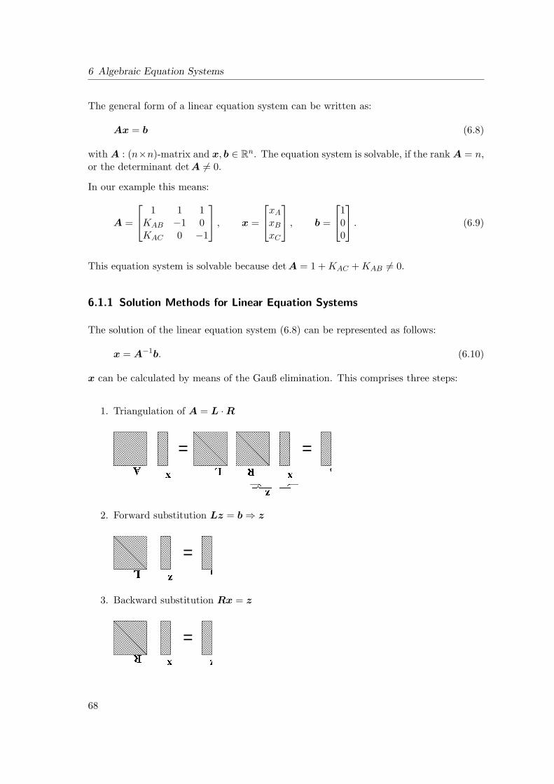
6 Algebraic Equation Systems
The general form of a linear equation system can be written as:
Ax = b (6.8)
with A : (n×n)-matrix and x, b ∈ Rn. The equation system is solvable, if the rank A = n,or the determinant det A 6= 0.
In our example this means:
A =
1 1 1KAB −1 0KAC 0 −1
, x =
xA
xB
xC
, b =
100
. (6.9)
This equation system is solvable because detA = 1 + KAC + KAB 6= 0.
6.1.1 Solution Methods for Linear Equation Systems
The solution of the linear equation system (6.8) can be represented as follows:
x = A−1b. (6.10)
x can be calculated by means of the Gauß elimination. This comprises three steps:
1. Triangulation of A = L ·R
==
2. Forward substitution Lz = b ⇒ z
=
3. Backward substitution Rx = z
=
68
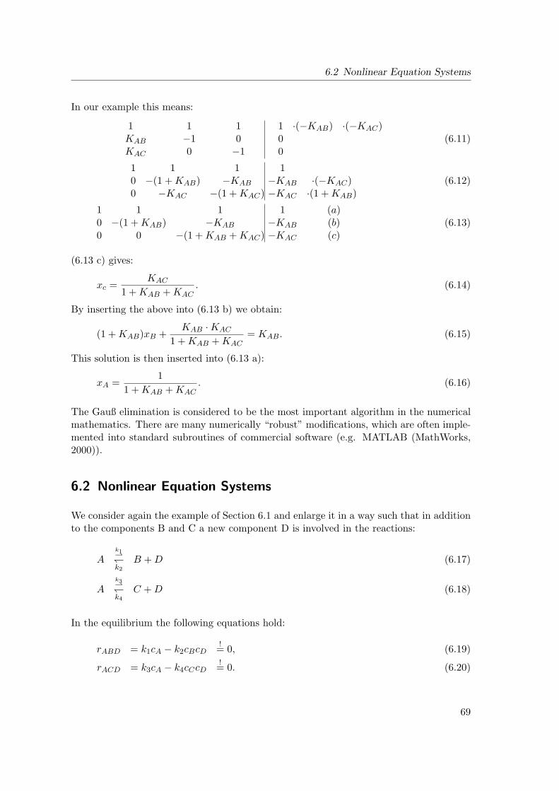
6.2 Nonlinear Equation Systems
In our example this means:
1 1 1KAB −1 0KAC 0 −1
1 ·(−KAB) ·(−KAC)00
(6.11)
1 1 10 −(1 + KAB) −KAB
0 −KAC −(1 + KAC)
1−KAB ·(−KAC)−KAC ·(1 + KAB)
(6.12)
1 1 10 −(1 + KAB) −KAB
0 0 −(1 + KAB + KAC)
1 (a)−KAB (b)−KAC (c)
(6.13)
(6.13 c) gives:
xc =KAC
1 + KAB + KAC. (6.14)
By inserting the above into (6.13 b) we obtain:
(1 + KAB)xB +KAB ·KAC
1 + KAB + KAC= KAB. (6.15)
This solution is then inserted into (6.13 a):
xA =1
1 + KAB + KAC. (6.16)
The Gauß elimination is considered to be the most important algorithm in the numericalmathematics. There are many numerically “robust” modifications, which are often imple-mented into standard subroutines of commercial software (e.g. MATLAB (MathWorks,2000)).
6.2 Nonlinear Equation Systems
We consider again the example of Section 6.1 and enlarge it in a way such that in additionto the components B and C a new component D is involved in the reactions:
Ak1k2
B + D (6.17)
Ak3k4
C + D (6.18)
In the equilibrium the following equations hold:
rABD = k1cA − k2cBcD!= 0, (6.19)
rACD = k3cA − k4cCcD!= 0. (6.20)
69
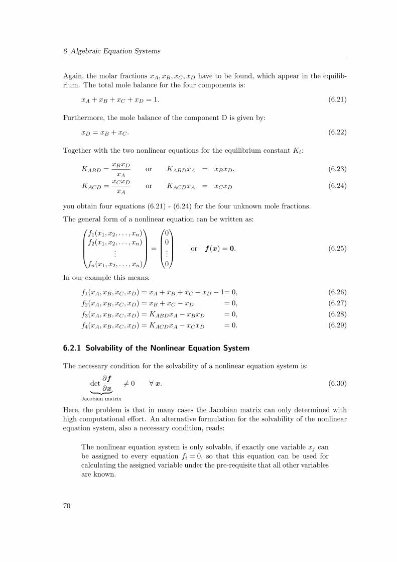
6 Algebraic Equation Systems
Again, the molar fractions xA, xB, xC , xD have to be found, which appear in the equilib-rium. The total mole balance for the four components is:
xA + xB + xC + xD = 1. (6.21)
Furthermore, the mole balance of the component D is given by:
xD = xB + xC . (6.22)
Together with the two nonlinear equations for the equilibrium constant Ki:
KABD =xBxD
xAor KABDxA = xBxD, (6.23)
KACD =xCxD
xAor KACDxA = xCxD (6.24)
you obtain four equations (6.21) - (6.24) for the four unknown mole fractions.
The general form of a nonlinear equation can be written as:f1(x1, x2, . . . , xn)f2(x1, x2, . . . , xn)
...fn(x1, x2, . . . , xn)
=
00...0
or f(x) = 0. (6.25)
In our example this means:
f1(xA, xB, xC , xD) = xA + xB + xC + xD − 1= 0, (6.26)f2(xA, xB, xC , xD) = xB + xC − xD = 0, (6.27)f3(xA, xB, xC , xD) = KABDxA − xBxD = 0, (6.28)f4(xA, xB, xC , xD) = KACDxA − xCxD = 0. (6.29)
6.2.1 Solvability of the Nonlinear Equation System
The necessary condition for the solvability of a nonlinear equation system is:
det∂f
∂x︸ ︷︷ ︸Jacobian matrix
6= 0 ∀ x. (6.30)
Here, the problem is that in many cases the Jacobian matrix can only determined withhigh computational effort. An alternative formulation for the solvability of the nonlinearequation system, also a necessary condition, reads:
The nonlinear equation system is only solvable, if exactly one variable xj canbe assigned to every equation fi = 0, so that this equation can be used forcalculating the assigned variable under the pre-requisite that all other variablesare known.
70
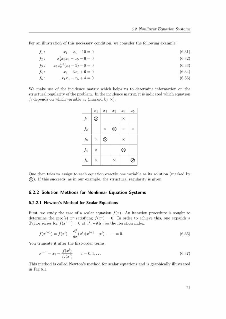
6.2 Nonlinear Equation Systems
For an illustration of this necessary condition, we consider the following example:
f1 : x1 + x4 − 10 = 0 (6.31)
f2 : x22x3x4 − x5 − 6 = 0 (6.32)
f3 : x1x1,72 (x4 − 5)− 8 = 0 (6.33)
f4 : x4 − 3x1 + 6 = 0 (6.34)f5 : x1x3 − x5 + 4 = 0 (6.35)
We make use of the incidence matrix which helps us to determine information on thestructural regularity of the problem. In the incidence matrix, it is indicated which equationfi depends on which variable xi (marked by ×).
x1 x2 x3 x4 x5
f1⊗
×
f2 ×⊗
× ×
f3 ×⊗
×
f4 ×⊗
f5 × ×⊗
One then tries to assign to each equation exactly one variable as its solution (marked by⊗). If this succeeds, as in our example, the structural regularity is given.
6.2.2 Solution Methods for Nonlinear Equation Systems
6.2.2.1 Newton’s Method for Scalar Equations
First, we study the case of a scalar equation f(x). An iteration procedure is sought todetermine the zero(s) x∗ satisfying f(x∗) = 0. In order to achieve this, one expands aTaylor series for f(xi+1) = 0 at xi, with i as the iteration index:
f(xi+1) = f(xi) +df
dx(xi)(xi+1 − xi) + · · · = 0. (6.36)
You truncate it after the first-order terms:
xi+1 = xi −f(xi)fx(xi)
i = 0, 1, . . . (6.37)
This method is called Newton’s method for scalar equations and is graphically illustratedin Fig 6.1.
71
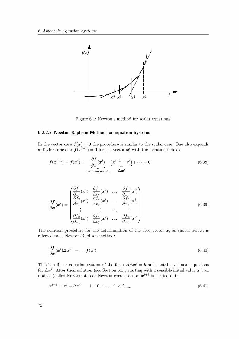
6 Algebraic Equation Systems
x
f(x)
x3 x2 x1x*
Figure 6.1: Newton’s method for scalar equations.
6.2.2.2 Newton-Raphson Method for Equation Systems
In the vector case f(x) = 0 the procedure is similar to the scalar case. One also expandsa Taylor series for f(xi+1) = 0 for the vector xi with the iteration index i:
f(xi+1) = f(xi) +∂f
∂x(xi)︸ ︷︷ ︸
Jacobian matrix
(xi+1 − xi)︸ ︷︷ ︸∆xi
+ · · · = 0 (6.38)
∂f
∂x(xi) =
∂f1
∂x1(xi)
∂f1
∂x2(xi) . . .
∂f1
∂xn(xi)
∂f2
∂x1(xi)
∂f2
∂x2(xi) . . .
∂f2
∂xn(xi)
......
. . ....
∂fn
∂x1(xi)
∂fn
∂x2(xi) . . .
∂fn
∂xn(xi)
(6.39)
The solution procedure for the determination of the zero vector x, as shown below, isreferred to as Newton-Raphson method:
∂f
∂x(xi)∆xi = −f(xi). (6.40)
This is a linear equation system of the form A∆xi = b and contains n linear equationsfor ∆xi. After their solution (see Section 6.1), starting with a sensible initial value x0, anupdate (called Newton step or Newton correction) of xi+1 is carried out:
xi+1 = xi + ∆xi i = 0, 1, . . . , i0 < imax (6.41)
72
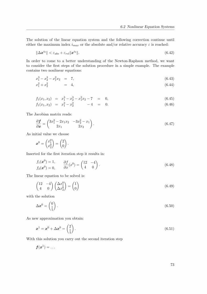
6.2 Nonlinear Equation Systems
The solution of the linear equation system and the following correction continue untileither the maximum index imax or the absolute and/or relative accuracy ε is reached:
‖∆xi0‖ < εabs + εrel‖xi0‖. (6.42)
In order to come to a better understanding of the Newton-Raphson method, we wantto consider the first steps of the solution procedure in a simple example. The examplecontains two nonlinear equations:
x31 − x3
2 − x21x2 = 7, (6.43)
x21 + x2
2 = 4, (6.44)
f1(x1, x2) = x31 − x3
2 − x21x2 − 7 = 0, (6.45)
f1(x1, x2) = x21 − x2
2 − 4 = 0. (6.46)
The Jacobian matrix reads:
∂f
∂x=
(3x2
1 − 2x1x2 −3x22 − x1
2x1 2x2
). (6.47)
As initial value we choose
x0 =(
x01
x02
)=
(20
).
Inserted for the first iteration step it results in:
f1(x0) = 1,
f2(x0) = 0,
∂f
∂x(x0) =
(12 −44 0
). (6.48)
The linear equation to be solved is:(12 −44 0
) (∆x0
1
∆x02
)=
(10
)(6.49)
with the solution
∆x0 =(
014
). (6.50)
As new approximation you obtain:
x1 = x0 + ∆x0 =(
214
). (6.51)
With this solution you carry out the second iteration step
f(x1) = . . .
73
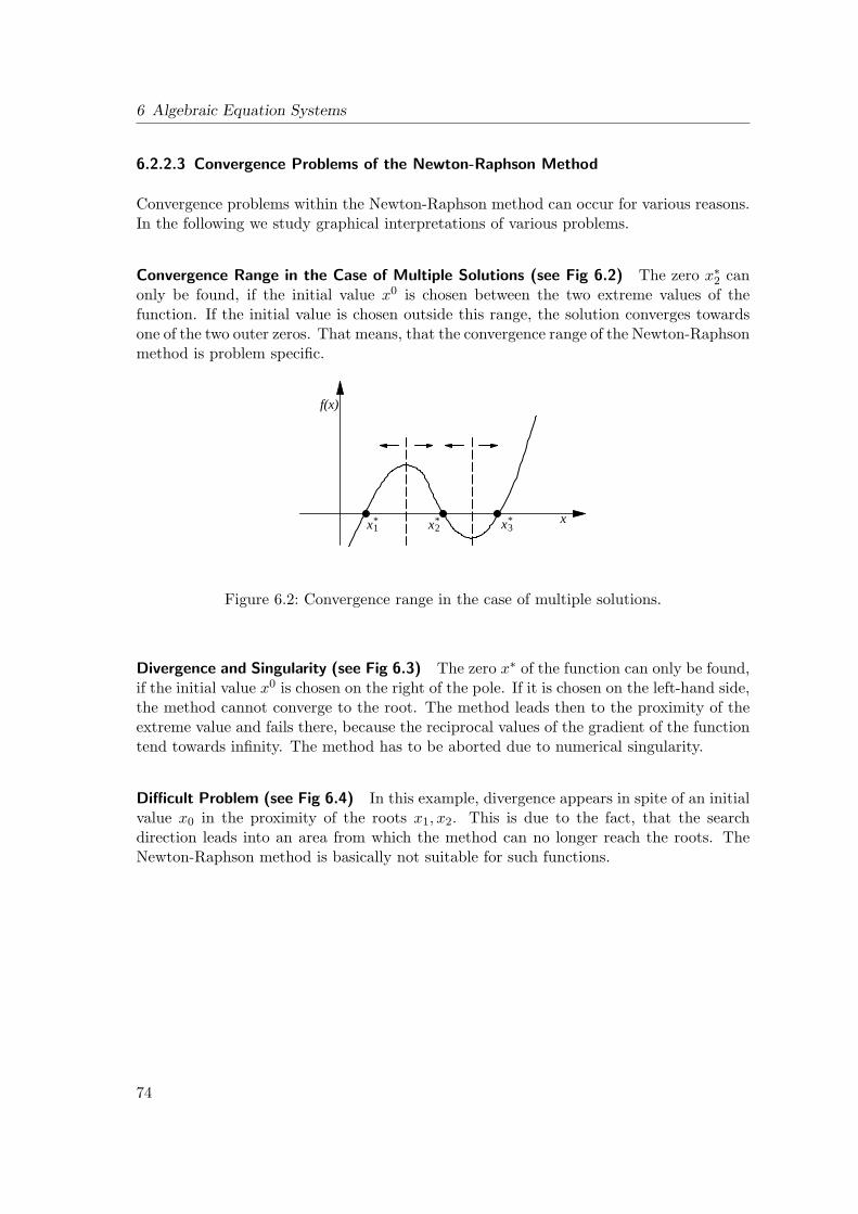
6 Algebraic Equation Systems
6.2.2.3 Convergence Problems of the Newton-Raphson Method
Convergence problems within the Newton-Raphson method can occur for various reasons.In the following we study graphical interpretations of various problems.
Convergence Range in the Case of Multiple Solutions (see Fig 6.2) The zero x∗2 canonly be found, if the initial value x0 is chosen between the two extreme values of thefunction. If the initial value is chosen outside this range, the solution converges towardsone of the two outer zeros. That means, that the convergence range of the Newton-Raphsonmethod is problem specific.
xx*1 x*
2 x*3
f(x)
Figure 6.2: Convergence range in the case of multiple solutions.
Divergence and Singularity (see Fig 6.3) The zero x∗ of the function can only be found,if the initial value x0 is chosen on the right of the pole. If it is chosen on the left-hand side,the method cannot converge to the root. The method leads then to the proximity of theextreme value and fails there, because the reciprocal values of the gradient of the functiontend towards infinity. The method has to be aborted due to numerical singularity.
Difficult Problem (see Fig 6.4) In this example, divergence appears in spite of an initialvalue x0 in the proximity of the roots x1, x2. This is due to the fact, that the searchdirection leads into an area from which the method can no longer reach the roots. TheNewton-Raphson method is basically not suitable for such functions.
74
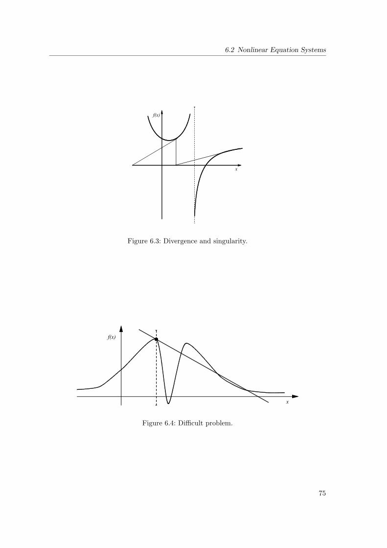
6.2 Nonlinear Equation Systems
Figure 6.3: Divergence and singularity.
Figure 6.4: Difficult problem.
75

6 Algebraic Equation Systems
76
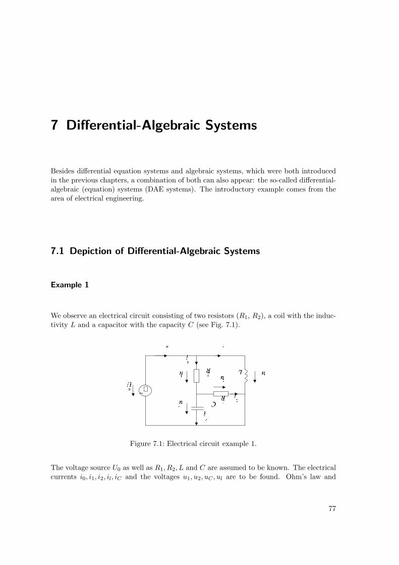
7 Differential-Algebraic Systems
Besides differential equation systems and algebraic systems, which were both introducedin the previous chapters, a combination of both can also appear: the so-called differential-algebraic (equation) systems (DAE systems). The introductory example comes from thearea of electrical engineering.
7.1 Depiction of Differential-Algebraic Systems
Example 1
We observe an electrical circuit consisting of two resistors (R1, R2), a coil with the induc-tivity L and a capacitor with the capacity C (see Fig. 7.1).
+
Figure 7.1: Electrical circuit example 1.
The voltage source U0 as well as R1, R2, L and C are assumed to be known. The electricalcurrents i0, i1, i2, il, iC and the voltages u1, u2, uC , ul are to be found. Ohm’s law and
77
7 Differential-Algebraic Systems
Kirchhoff’s loop rule yields the model equations:
u1 = R1 · i1 (7.1)u2 = R2 · i2 (7.2)
uL = L · diLdt
(7.3)
iC = C · duC
dt(7.4)
U0 = u1 + uc (7.5)uC = u2 (7.6)uL = u1 + u2 (7.7)i0 = i1 + iL (7.8)i1 = i2 + iC (7.9)
This leads to an equation system, which consists of two differential equations (7.3), (7.4),and seven algebraic equations. Therefore, it is called a differential-algebraic system.
For the representation of differential-algebraic systems several different characteristic classescan be distinguished.
7.1.1 General Nonlinear Implicit Form
The general implicit form of a differential-algebraic system is:
0 = F (z,z,d), (7.10)
with
z ∈ Rn : state vector, (7.11)d ∈ Rd : vector of the input quantities and parameter. (7.12)
The system can be transformed to:
0 = f(z,z,d) f ∈ Rn−k, g ∈ Rk (7.13)0 = g(z,d) (7.14)
(7.13) comprises a system of ordinary differential equations, (7.14) comprises a system of(non-) linear algebraic equations.
78
7.1 Depiction of Differential-Algebraic Systems
7.1.2 Explicit Differential-Algebraic System
The explicit differential-algebraic system is a special case of 7.1.1 and occurs often e.g. inchemical engineering:
x = f(x,y,d), x : vector of the differential state variable, (7.15)0 = g(x,y,d), y : vector of the algebraic state variable. (7.16)
y consists of variables, which are not differentiated. Therefore, the vector z can be dividedinto differential and algebraic variables. Example 1 is an example for such an explicit DAEsystem. This can be easily seen after the following transformations:
diLdt
=1L
uL
duC
dt=
1C
iC
x = f(x,y,d),
g1 : 0 = u1 −R1 · i1g2 : 0 = u2 −R2 · i2g3 : 0 = U0 − u1 − uC
g4 : 0 = uC − u2
g5 : 0 = uL − u1 − u2
g6 : 0 = i0 − i1 − iL
g7 : 0 = i1 − i2 − iC
0 = g(x,y,d),
with
x = [iL, uC ]T , (7.17)y = [i0, i1, i2, iC , u1, u2, uL]T , (7.18)d = [U0, R1, R2, L, C]T . (7.19)
7.1.3 Linear Differential-Algebraic System
In addition to nonlinear differential-algebraic systems, linear differential-algebraic systemswith constant coefficients play a special role:
Mz = Az + Bd, z =[x,y
]T. (7.20)
You obtain such models e.g. through linearization of nonlinear implicit or explicit differential-algebraic systems. Many control engineering and system theoretical concepts are basedon systems of the form (7.20).
79
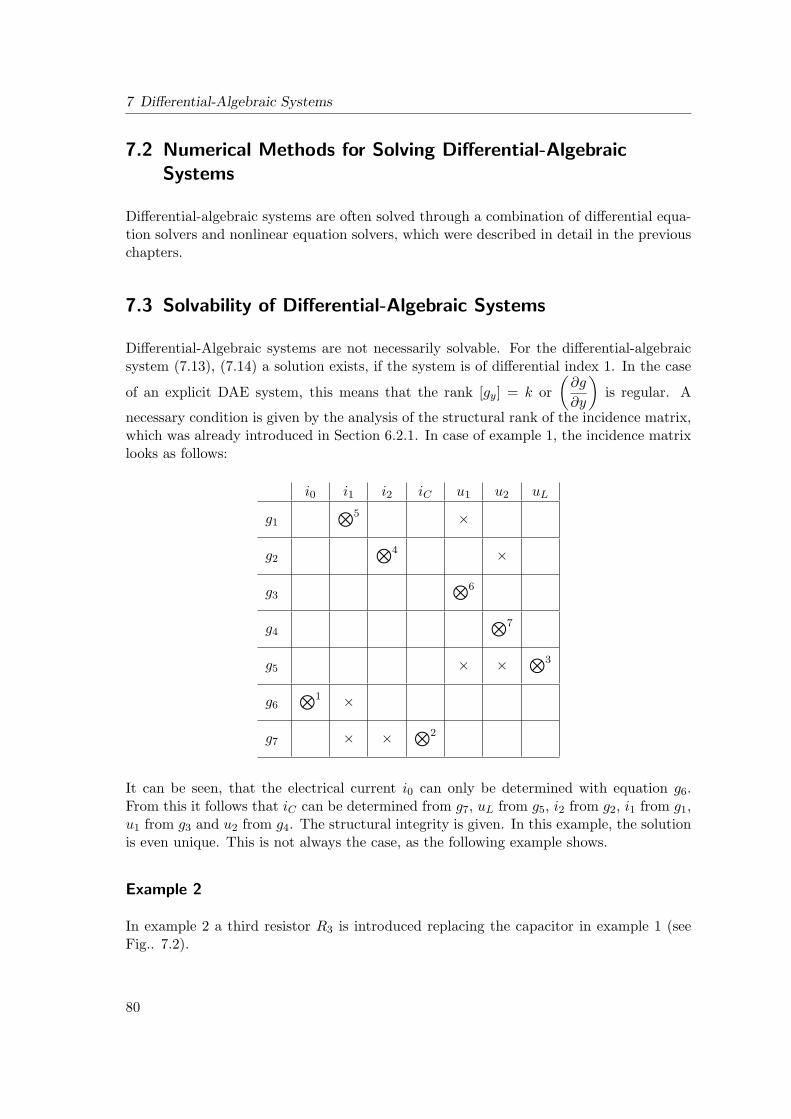
7 Differential-Algebraic Systems
7.2 Numerical Methods for Solving Differential-AlgebraicSystems
Differential-algebraic systems are often solved through a combination of differential equa-tion solvers and nonlinear equation solvers, which were described in detail in the previouschapters.
7.3 Solvability of Differential-Algebraic Systems
Differential-Algebraic systems are not necessarily solvable. For the differential-algebraicsystem (7.13), (7.14) a solution exists, if the system is of differential index 1. In the case
of an explicit DAE system, this means that the rank [gy] = k or(
∂g
∂y
)is regular. A
necessary condition is given by the analysis of the structural rank of the incidence matrix,which was already introduced in Section 6.2.1. In case of example 1, the incidence matrixlooks as follows:
i0 i1 i2 iC u1 u2 uL
g1⊗5 ×
g2⊗4 ×
g3⊗6
g4⊗7
g5 × ×⊗3
g6⊗1 ×
g7 × ×⊗2
It can be seen, that the electrical current i0 can only be determined with equation g6.From this it follows that iC can be determined from g7, uL from g5, i2 from g2, i1 from g1,u1 from g3 and u2 from g4. The structural integrity is given. In this example, the solutionis even unique. This is not always the case, as the following example shows.
Example 2
In example 2 a third resistor R3 is introduced replacing the capacitor in example 1 (seeFig.. 7.2).
80
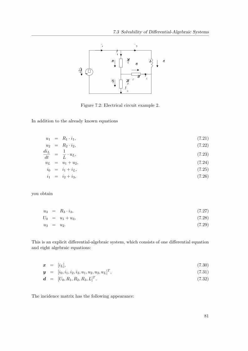
7.3 Solvability of Differential-Algebraic Systems
+
Figure 7.2: Electrical circuit example 2.
In addition to the already known equations
u1 = R1 · i1, (7.21)u2 = R2 · i2, (7.22)
diLdt
=1L· uL, (7.23)
uL = u1 + u2, (7.24)i0 = i1 + iL, (7.25)i1 = i2 + i3, (7.26)
you obtain
u3 = R3 · i3, (7.27)U0 = u1 + u3, (7.28)u3 = u2. (7.29)
This is an explicit differential-algebraic system, which consists of one differential equationand eight algebraic equations:
x = [iL], (7.30)y = [i0, i1, i2, i3, u1, u2, u3, uL]T , (7.31)d = [U0, R1, R2, R3, L]T . (7.32)
The incidence matrix has the following appearance:
81
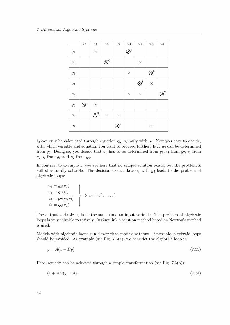
7 Differential-Algebraic Systems
i0 i1 i2 i3 u1 u2 u3 uL
g1 ×⊗4
g2⊗6 ×
g3 ×⊗3
g4⊗8 ×
g5 × ×⊗2
g6⊗1 ×
g7⊗5 × ×
g8⊗7 ×
i0 can only be calculated through equation g6, uL only with g5. Now you have to decide,with which variable and equation you want to proceed further. E.g. u3 can be determinedfrom g3. Doing so, you decide that u1 has to be determined from g1, i1 from g7, i2 fromg2, il from g8 and u2 from g4.
In contrast to example 1, you see here that no unique solution exists, but the problem isstill structurally solvable. The decision to calculate u3 with g3 leads to the problem ofalgebraic loops:
u3 = g3(u1)u1 = g1(i1)i1 = g7(i2, i3)i3 = g8(u3)
⇒ u3 = g(u3, . . . )
The output variable u3 is at the same time an input variable. The problem of algebraicloops is only solvable iteratively. In Simulink a solution method based on Newton’s methodis used.
Models with algebraic loops run slower than models without. If possible, algebraic loopsshould be avoided. As example (see Fig. 7.3(a)) we consider the algebraic loop in
y = A(x−By) (7.33)
Here, remedy can be achieved through a simple transformation (see Fig. 7.3(b)):
(1 + AB)y = Ax (7.34)
82
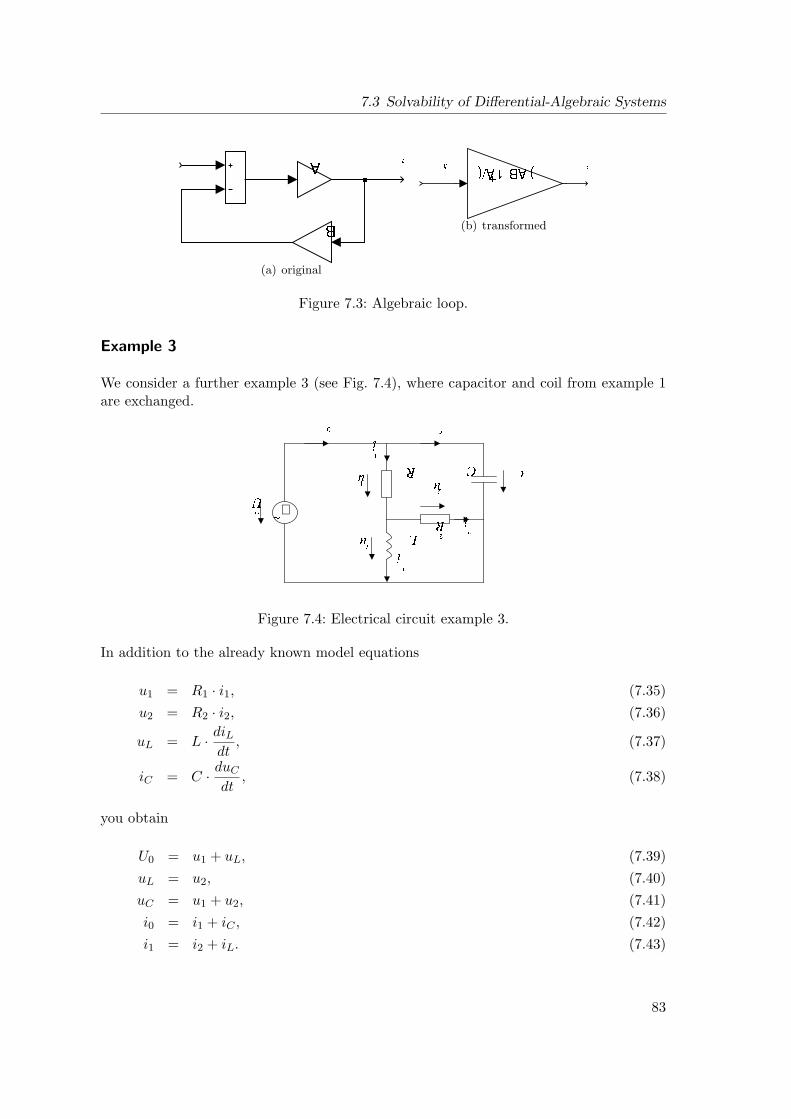
7.3 Solvability of Differential-Algebraic Systems
(a) original
(b) transformed
Figure 7.3: Algebraic loop.
Example 3
We consider a further example 3 (see Fig. 7.4), where capacitor and coil from example 1are exchanged.
+
Figure 7.4: Electrical circuit example 3.
In addition to the already known model equations
u1 = R1 · i1, (7.35)u2 = R2 · i2, (7.36)
uL = L · diLdt
, (7.37)
iC = C · duC
dt, (7.38)
you obtain
U0 = u1 + uL, (7.39)uL = u2, (7.40)uC = u1 + u2, (7.41)i0 = i1 + iC , (7.42)i1 = i2 + iL. (7.43)
83
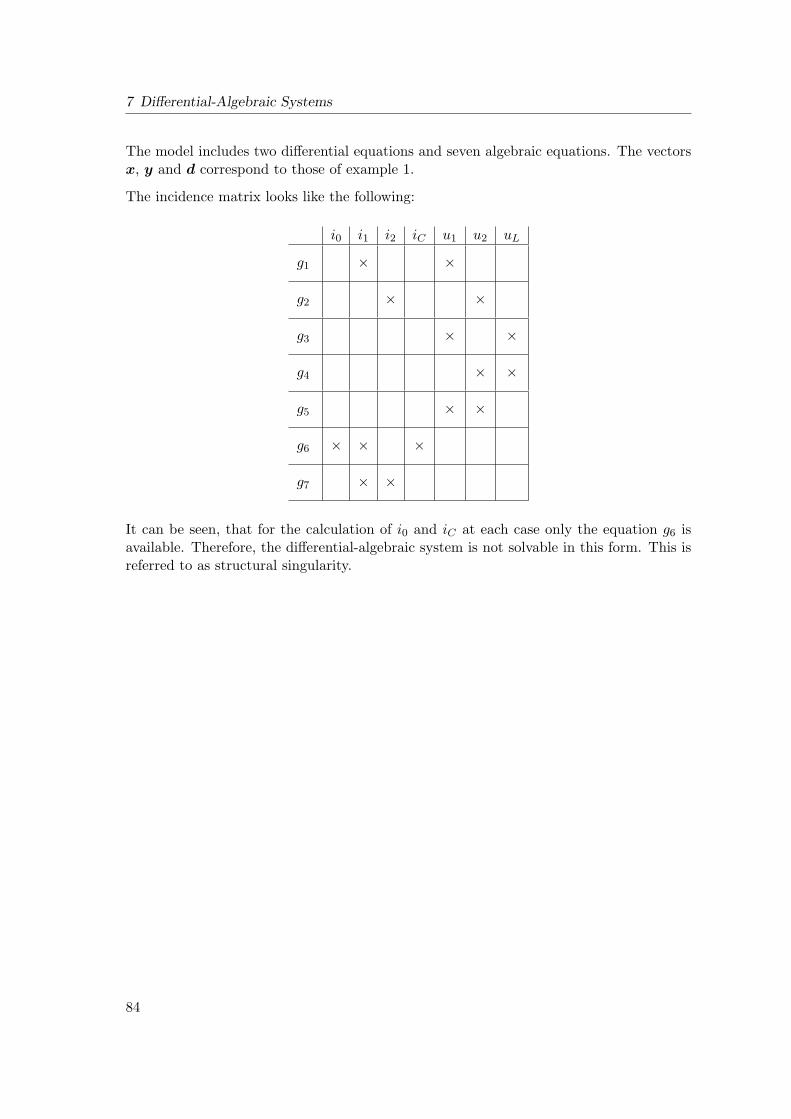
7 Differential-Algebraic Systems
The model includes two differential equations and seven algebraic equations. The vectorsx, y and d correspond to those of example 1.
The incidence matrix looks like the following:
i0 i1 i2 iC u1 u2 uL
g1 × ×
g2 × ×
g3 × ×
g4 × ×
g5 × ×
g6 × × ×
g7 × ×
It can be seen, that for the calculation of i0 and iC at each case only the equation g6 isavailable. Therefore, the differential-algebraic system is not solvable in this form. This isreferred to as structural singularity.
84
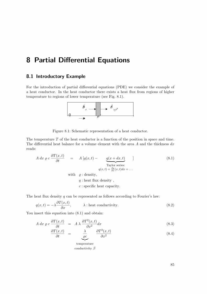
8 Partial Differential Equations
8.1 Introductory Example
For the introduction of partial differential equations (PDE) we consider the example ofa heat conductor. In the heat conductor there exists a heat flux from regions of highertemperature to regions of lower temperature (see Fig. 8.1).
+
Figure 8.1: Schematic representation of a heat conductor.
The temperature T of the heat conductor is a function of the position in space and time.The differential heat balance for a volume element with the area A and the thickness dxreads:
A dx % c∂T (x, t)
∂t= A [q(x, t)− q(x + dx, t)︸ ︷︷ ︸
Taylor series:
q(x, t) + ∂q∂x
(x, t)dx + . . .
] (8.1)
with % : density,
q : heat flux density ,
c : specific heat capacity.
The heat flux density q can be represented as follows according to Fourier’s law:
q(x, t) = −λ∂T (x, t)
∂x, λ : heat conductivity. (8.2)
You insert this equation into (8.1) and obtain:
A dx % c∂T (x, t)
∂t= A λ
∂T 2(x, t)∂x2
dx (8.3)
∂T (x, t)∂t
=λ
%c︸︷︷︸temperature
conductivity β
∂T 2(x, t)∂x2
(8.4)
85
8 Partial Differential Equations
(8.4) is the heat conductivity equation. This is a partial differential equation, because itcontains derivatives with respect to space as well as derivatives with respect to time.
For a complete mathematical model additional boundary conditions have to be determined.The number of the conditions for every independent variable (x, t) corresponds to the orderof its highest derivative.
For the time t the first derivative is∂T
∂t. Therefore one boundary condition for t is
needed, e.g. an initial condition: T (x, t0) = T0(x), the temperature profile along the heatconductor at time t0.
x occurs in the second derivative∂2T
∂x2. So two boundary conditions are needed for x.
Examples for these are:
a) Dirichlet conditions
T (0, t) = T1(t) (8.5)T (l, t) = T2(t) (8.6)
b) Neumann conditions
∂T (0, t)∂x
= 0 (8.7)
∂T (l, t)∂x
= 0 (8.8)
c) Robbins conditions
∂T (0, t)∂x
= 0 (8.9)
λ∂T (l, t)
∂x= ε(T 4
a − T (l, t)4) (8.10)
8.2 Representation of Partial Differential Equations
The highest order of derivative occurring in a (partial) differential equation is called theorder of the differential equation. The general form of a partial differential equation ofsecond order (z = z(x, t)) reads:
a(·)ztt + 2b(·)ztx + c(·)zxx + d(·)zt + e(·)zx + f(·)z + g(·) = 0 (8.11)
You distinguish between linear, quasi-linear and nonlinear partial differential equations:
linear: a(·), b(·), c(·) constant or function of t and x,quasi-linear: a(·), b(·), c(·) function of t, x, z, zt, zx,nonlinear: in all other cases.
86
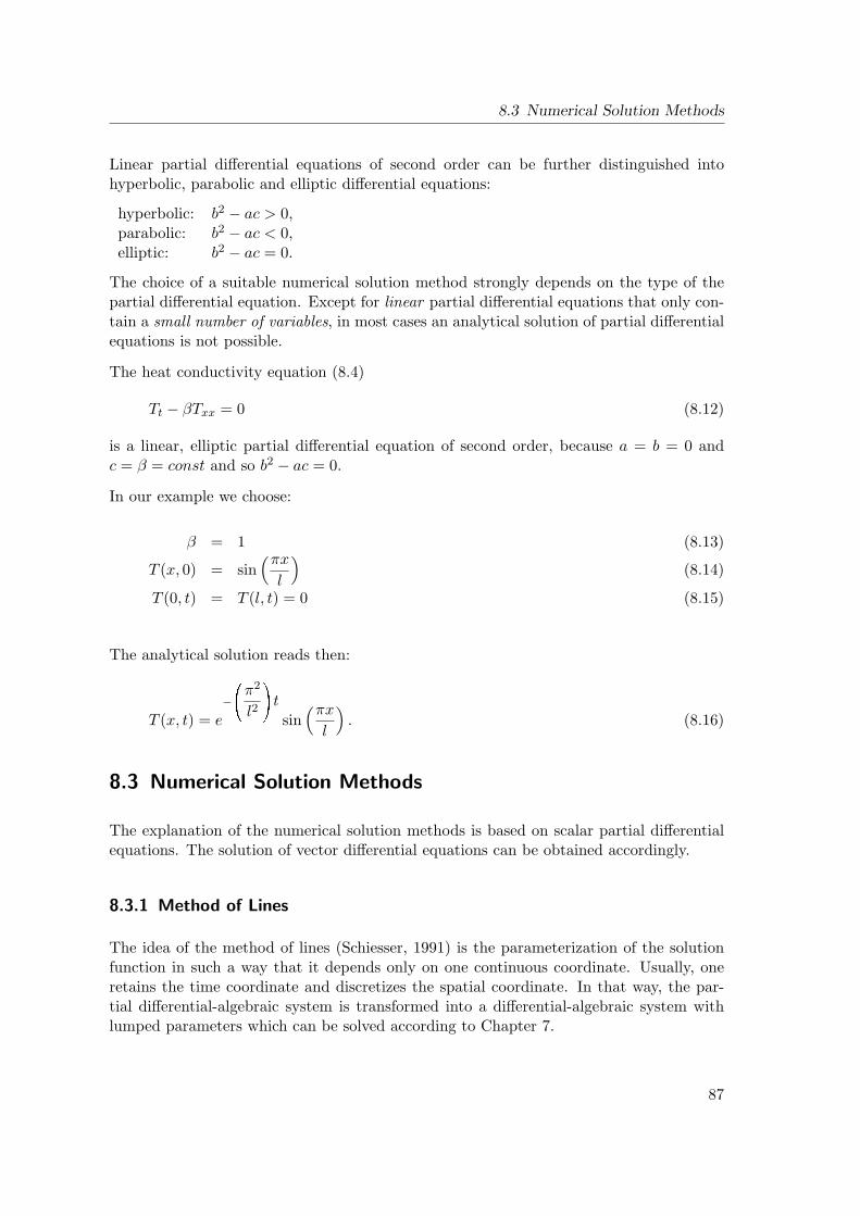
8.3 Numerical Solution Methods
Linear partial differential equations of second order can be further distinguished intohyperbolic, parabolic and elliptic differential equations:
hyperbolic: b2 − ac > 0,parabolic: b2 − ac < 0,elliptic: b2 − ac = 0.
The choice of a suitable numerical solution method strongly depends on the type of thepartial differential equation. Except for linear partial differential equations that only con-tain a small number of variables, in most cases an analytical solution of partial differentialequations is not possible.
The heat conductivity equation (8.4)
Tt − βTxx = 0 (8.12)
is a linear, elliptic partial differential equation of second order, because a = b = 0 andc = β = const and so b2 − ac = 0.
In our example we choose:
β = 1 (8.13)
T (x, 0) = sin(πx
l
)(8.14)
T (0, t) = T (l, t) = 0 (8.15)
The analytical solution reads then:
T (x, t) = e−
0@π2
l2
1At
sin(πx
l
). (8.16)
8.3 Numerical Solution Methods
The explanation of the numerical solution methods is based on scalar partial differentialequations. The solution of vector differential equations can be obtained accordingly.
8.3.1 Method of Lines
The idea of the method of lines (Schiesser, 1991) is the parameterization of the solutionfunction in such a way that it depends only on one continuous coordinate. Usually, oneretains the time coordinate and discretizes the spatial coordinate. In that way, the par-tial differential-algebraic system is transformed into a differential-algebraic system withlumped parameters which can be solved according to Chapter 7.
87
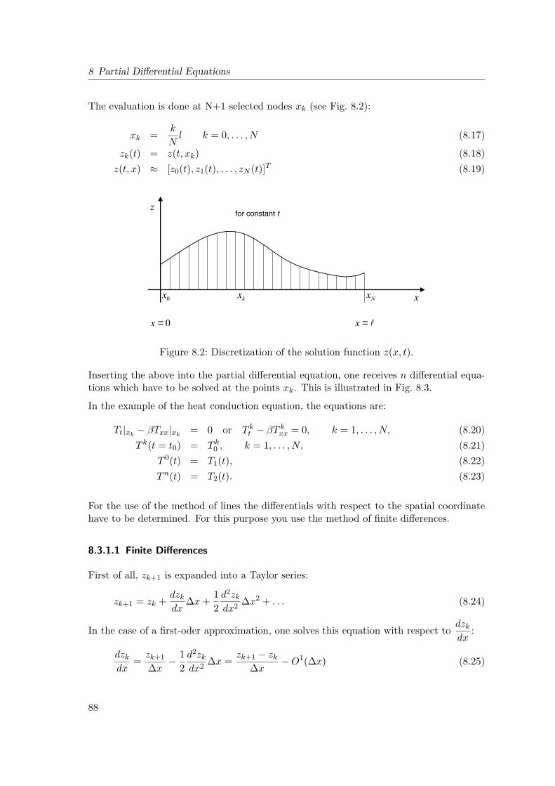
8 Partial Differential Equations
The evaluation is done at N+1 selected nodes xk (see Fig. 8.2):
xk =k
Nl k = 0, . . . , N (8.17)
zk(t) = z(t, xk) (8.18)z(t, x) ≈ [z0(t), z1(t), . . . , zN (t)]T (8.19)
==
Figure 8.2: Discretization of the solution function z(x, t).
Inserting the above into the partial differential equation, one receives n differential equa-tions which have to be solved at the points xk. This is illustrated in Fig. 8.3.
In the example of the heat conduction equation, the equations are:
Tt|xk− βTxx|xk
= 0 or T kt − βT k
xx = 0, k = 1, . . . , N, (8.20)T k(t = t0) = T k
0 , k = 1, . . . , N, (8.21)T 0(t) = T1(t), (8.22)Tn(t) = T2(t). (8.23)
For the use of the method of lines the differentials with respect to the spatial coordinatehave to be determined. For this purpose you use the method of finite differences.
8.3.1.1 Finite Differences
First of all, zk+1 is expanded into a Taylor series:
zk+1 = zk +dzk
dx∆x +
12
d2zk
dx2∆x2 + . . . (8.24)
In the case of a first-oder approximation, one solves this equation with respect todzk
dx:
dzk
dx=
zk+1
∆x− 1
2d2zk
dx2∆x =
zk+1 − zk
∆x−O1(∆x) (8.25)
88
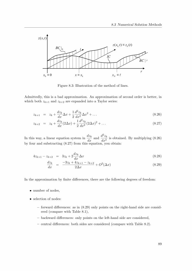
8.3 Numerical Solution Methods
=
= = =
Figure 8.3: Illustration of the method of lines.
Admittedly, this is a bad approximation. An approximation of second order is better, inwhich both zk+1 and zk+2 are expanded into a Taylor series:
zk+1 = zk +dzk
dx∆x +
12
d2zk
dx2∆x2 + . . . (8.26)
zk+2 = zk +dzk
dx(2∆x) +
12
d2zk
dx2(2∆x)2 + . . . (8.27)
In this way, a linear equation system indzk
dxand
d2zk
dx2is obtained. By multiplying (8.26)
by four and substracting (8.27) from this equation, you obtain:
4zk+1 − zk+2 = 3zk + 2dzk
dx∆x (8.28)
dzk
dx=
−3zk + 4zk+1 − zk+2
2∆x+ O2(∆x) (8.29)
In the approximation by finite differences, there are the following degrees of freedom:
number of nodes,
selection of nodes:
– forward differences: as in (8.29) only points on the right-hand side are consid-ered (compare with Table 8.1),
– backward differences: only points on the left-hand side are considered,
– central differences: both sides are considered (compare with Table 8.2).
89
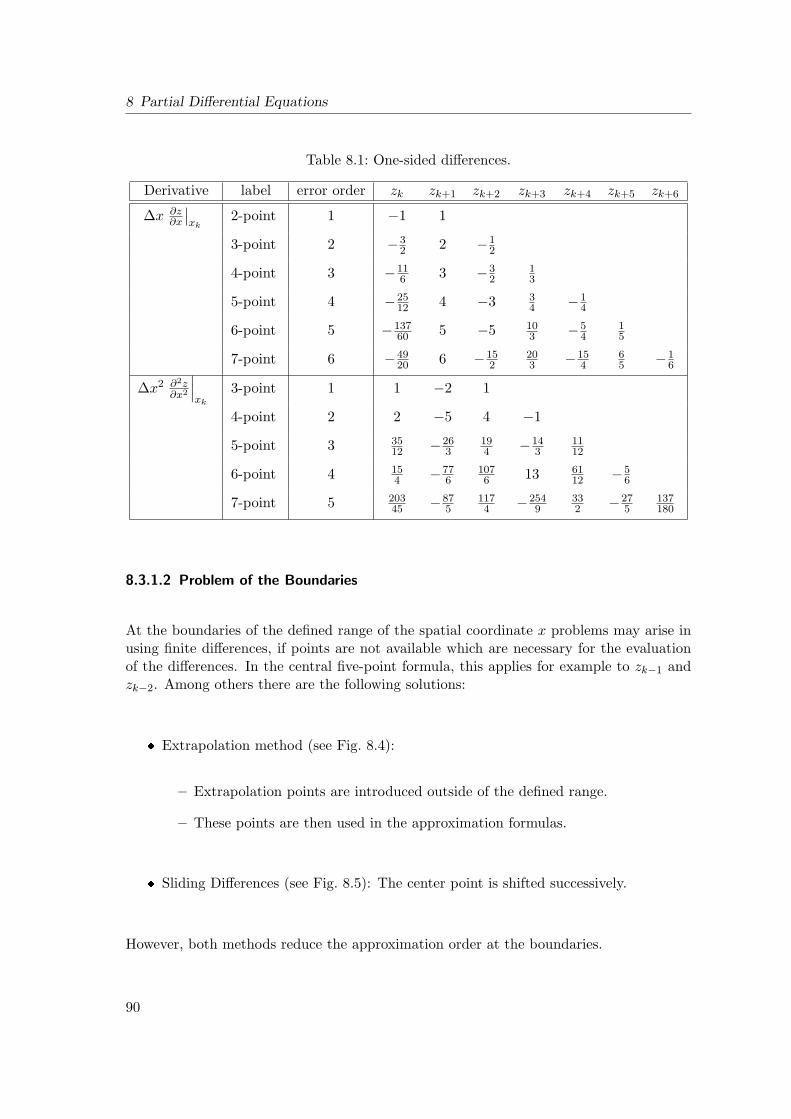
8 Partial Differential Equations
Table 8.1: One-sided differences.
Derivative label error order zk zk+1 zk+2 zk+3 zk+4 zk+5 zk+6
∆x ∂z∂x
∣∣xk
2-point 1 −1 1
3-point 2 −32 2 −1
2
4-point 3 −116 3 −3
213
5-point 4 −2512 4 −3 3
4 −14
6-point 5 −13760 5 −5 10
3 −54
15
7-point 6 −4920 6 −15
2203 −15
465 −1
6
∆x2 ∂2z∂x2
∣∣∣xk
3-point 1 1 −2 1
4-point 2 2 −5 4 −1
5-point 3 3512 −26
3194 −14
31112
6-point 4 154 −77
61076 13 61
12 −56
7-point 5 20345 −87
51174 −254
9332 −27
5137180
8.3.1.2 Problem of the Boundaries
At the boundaries of the defined range of the spatial coordinate x problems may arise inusing finite differences, if points are not available which are necessary for the evaluationof the differences. In the central five-point formula, this applies for example to zk−1 andzk−2. Among others there are the following solutions:
Extrapolation method (see Fig. 8.4):
– Extrapolation points are introduced outside of the defined range.
– These points are then used in the approximation formulas.
Sliding Differences (see Fig. 8.5): The center point is shifted successively.
However, both methods reduce the approximation order at the boundaries.
90
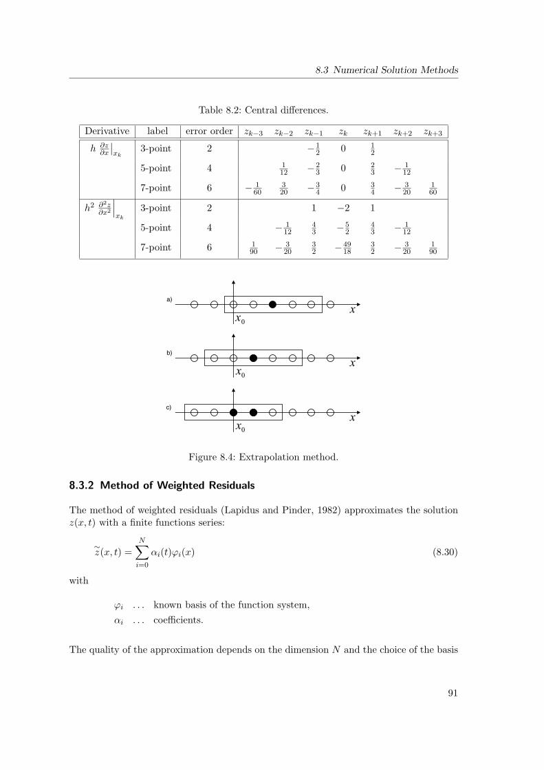
8.3 Numerical Solution Methods
Table 8.2: Central differences.
Derivative label error order zk−3 zk−2 zk−1 zk zk+1 zk+2 zk+3
h ∂z∂x
∣∣xk
3-point 2 −12 0 1
2
5-point 4 112 −2
3 0 23 − 1
12
7-point 6 − 160
320 −3
4 0 34 − 3
20160
h2 ∂2z∂x2
∣∣∣xk
3-point 2 1 −2 1
5-point 4 − 112
43 −5
243 − 1
12
7-point 6 190 − 3
2032 −49
1832 − 3
20190
Figure 8.4: Extrapolation method.
8.3.2 Method of Weighted Residuals
The method of weighted residuals (Lapidus and Pinder, 1982) approximates the solutionz(x, t) with a finite functions series:
∼z(x, t) =
N∑i=0
αi(t)ϕi(x) (8.30)
with
ϕi . . . known basis of the function system,
αi . . . coefficients.
The quality of the approximation depends on the dimension N and the choice of the basis
91
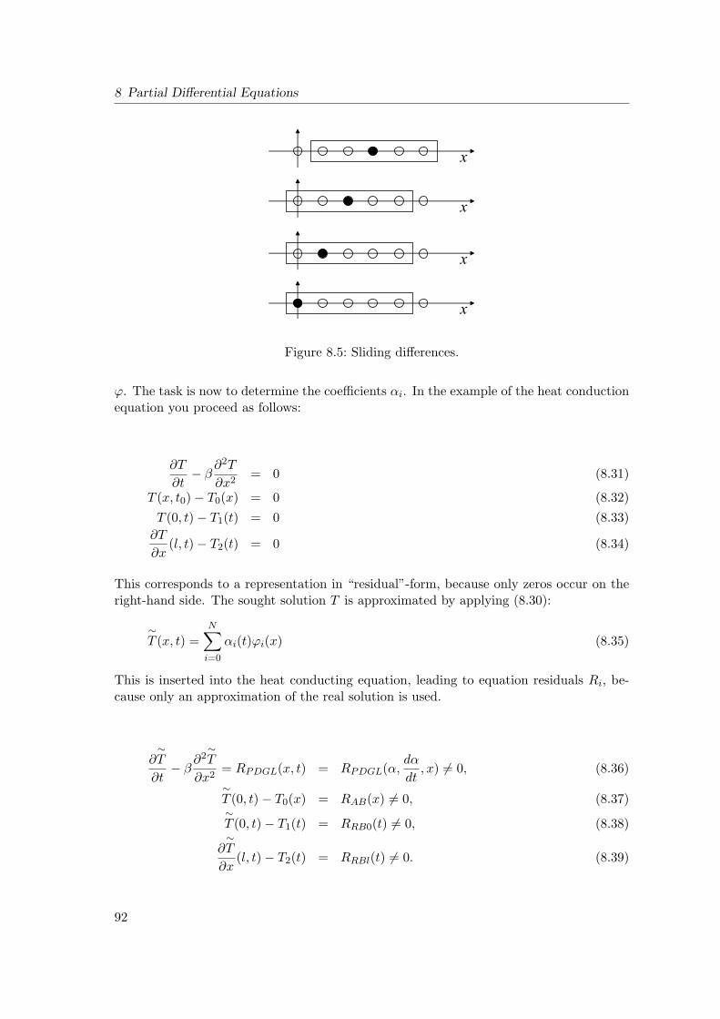
8 Partial Differential Equations
Figure 8.5: Sliding differences.
ϕ. The task is now to determine the coefficients αi. In the example of the heat conductionequation you proceed as follows:
∂T
∂t− β
∂2T
∂x2= 0 (8.31)
T (x, t0)− T0(x) = 0 (8.32)T (0, t)− T1(t) = 0 (8.33)
∂T
∂x(l, t)− T2(t) = 0 (8.34)
This corresponds to a representation in “residual”-form, because only zeros occur on theright-hand side. The sought solution T is approximated by applying (8.30):
∼T (x, t) =
N∑i=0
αi(t)ϕi(x) (8.35)
This is inserted into the heat conducting equation, leading to equation residuals Ri, be-cause only an approximation of the real solution is used.
∂∼T
∂t− β
∂2∼T
∂x2= RPDGL(x, t) = RPDGL(α,
dα
dt, x) 6= 0, (8.36)
∼T (0, t)− T0(x) = RAB(x) 6= 0, (8.37)∼T (0, t)− T1(t) = RRB0(t) 6= 0, (8.38)
∂∼T
∂x(l, t)− T2(t) = RRBl(t) 6= 0. (8.39)
92
8.3 Numerical Solution Methods
An approximation∼z is considered acceptable, if the suitable weighted equation residual R
disappears in the means over the considered range:
l∫0
R
(α,
dα
dt, x
)wi(x)dx = 0, i = 1, . . . , N. (8.40)
The choice of the weights wi characterizes the weighted residuals method. The three mostimportant methods are briefly introduced in the following sections (see Fig. 8.6).
8.3.2.1 Collocation Method
In the collocation method Dirac impulses are used as weighting functions:
l∫0
R
(α,
dα
dt, x
)δ(x− xi)dx = 0. (8.41)
As a consequence, you do not have to solve an integral system, but rather only an algebraicequation system:
R
(α,
dα
dt, xi
)= 0, i = 1, . . . , N. (8.42)
8.3.2.2 Control Volume Method
The control volume method uses weights wi only in an interval between two active nodes:
wi(x) =
1 if xi−1 < x < xi
0 elsewhere(8.43)
You obtain as the resulting equation system:
xi∫xi−1
R
(α,
dα
dt, x
)dx = 0, i = 1, . . . , N. (8.44)
8.3.2.3 Galerkin Method
The Galerkin method uses as weighting functions the sensitivity of the approximationfunction with respect to the parameters to be determined. In other words, the weightingfunctions are the basis functions:
wi(x) =∂∼z(x, t)∂αi
= ϕi(x), i = 1, . . . , N. (8.45)
93
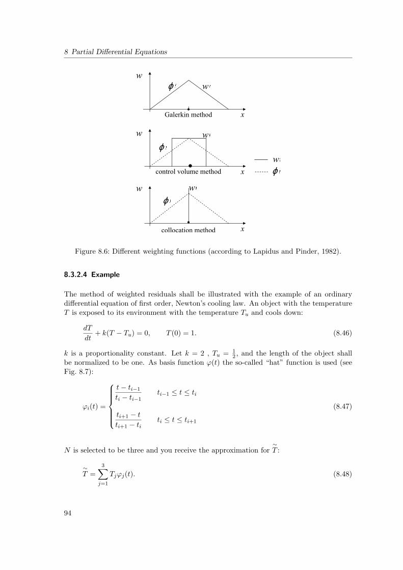
8 Partial Differential Equations
•
•
ϕ
ϕ
ϕ
ϕ
Figure 8.6: Different weighting functions (according to Lapidus and Pinder, 1982).
8.3.2.4 Example
The method of weighted residuals shall be illustrated with the example of an ordinarydifferential equation of first order, Newton’s cooling law. An object with the temperatureT is exposed to its environment with the temperature Tu and cools down:
dT
dt+ k(T − Tu) = 0, T (0) = 1. (8.46)
k is a proportionality constant. Let k = 2 , Tu = 12 , and the length of the object shall
be normalized to be one. As basis function ϕ(t) the so-called “hat” function is used (seeFig. 8.7):
ϕi(t) =
t− ti−1
ti − ti−1ti−1 ≤ t ≤ ti
ti+1 − t
ti+1 − titi ≤ t ≤ ti+1
(8.47)
N is selected to be three and you receive the approximation for∼T :
∼T =
3∑j=1
Tjϕj(t). (8.48)
94
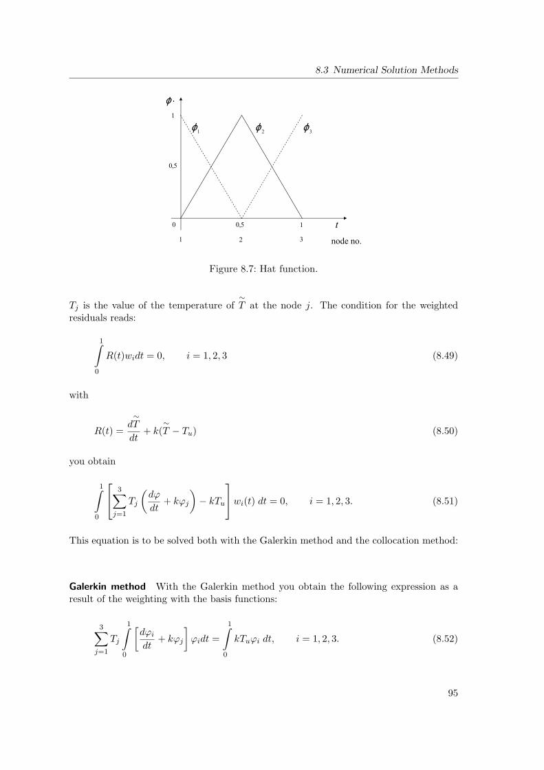
8.3 Numerical Solution Methods
ϕ
ϕ ϕ ϕ
Figure 8.7: Hat function.
Tj is the value of the temperature of∼T at the node j. The condition for the weighted
residuals reads:
1∫0
R(t)widt = 0, i = 1, 2, 3 (8.49)
with
R(t) =d∼T
dt+ k(
∼T − Tu) (8.50)
you obtain
1∫0
3∑j=1
Tj
(dϕ
dt+ kϕj
)− kTu
wi(t) dt = 0, i = 1, 2, 3. (8.51)
This equation is to be solved both with the Galerkin method and the collocation method:
Galerkin method With the Galerkin method you obtain the following expression as aresult of the weighting with the basis functions:
3∑j=1
Tj
1∫0
[dϕi
dt+ kϕj
]ϕidt =
1∫0
kTuϕi dt, i = 1, 2, 3. (8.52)
95
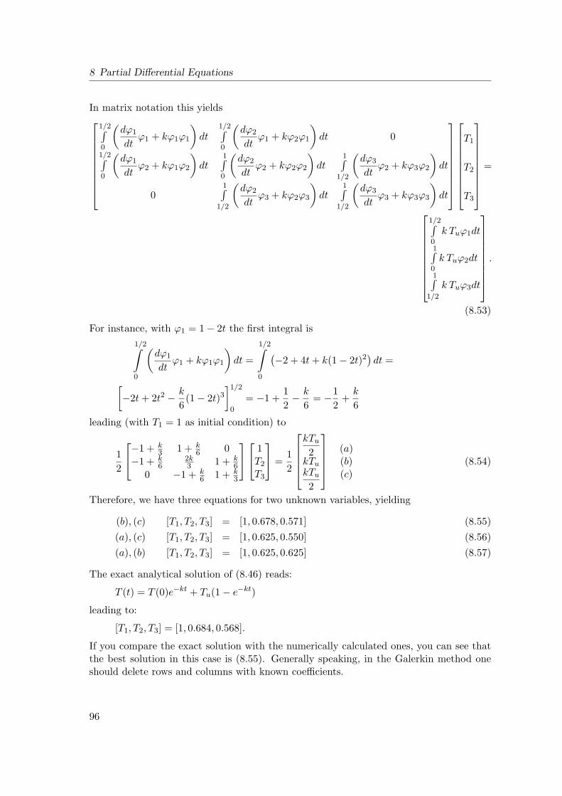
8 Partial Differential Equations
In matrix notation this yields
1/2∫0
(dϕ1
dtϕ1 + kϕ1ϕ1
)dt
1/2∫0
(dϕ2
dtϕ1 + kϕ2ϕ1
)dt 0
1/2∫0
(dϕ1
dtϕ2 + kϕ1ϕ2
)dt
1∫0
(dϕ2
dtϕ2 + kϕ2ϕ2
)dt
1∫1/2
(dϕ3
dtϕ2 + kϕ3ϕ2
)dt
01∫
1/2
(dϕ2
dtϕ3 + kϕ2ϕ3
)dt
1∫1/2
(dϕ3
dtϕ3 + kϕ3ϕ3
)dt
T1
T2
T3
=
1/2∫0
k Tuϕ1dt
1∫0
k Tuϕ2dt
1∫1/2
k Tuϕ3dt
.
(8.53)
For instance, with ϕ1 = 1− 2t the first integral is1/2∫0
(dϕ1
dtϕ1 + kϕ1ϕ1
)dt =
1/2∫0
(−2 + 4t + k(1− 2t)2
)dt =
[−2t + 2t2 − k
6(1− 2t)3
]1/2
0
= −1 +12− k
6= −1
2+
k
6
leading (with T1 = 1 as initial condition) to
12
−1 + k3 1 + k
6 0−1 + k
62k3 1 + k
6
0 −1 + k6 1 + k
3
1T2
T3
=12
kTu
2kTu
kTu
2
(a)(b)(c)
(8.54)
Therefore, we have three equations for two unknown variables, yielding
(b), (c) [T1, T2, T3] = [1, 0.678, 0.571] (8.55)(a), (c) [T1, T2, T3] = [1, 0.625, 0.550] (8.56)(a), (b) [T1, T2, T3] = [1, 0.625, 0.625] (8.57)
The exact analytical solution of (8.46) reads:
T (t) = T (0)e−kt + Tu(1− e−kt)
leading to:
[T1, T2, T3] = [1, 0.684, 0.568].
If you compare the exact solution with the numerically calculated ones, you can see thatthe best solution in this case is (8.55). Generally speaking, in the Galerkin method oneshould delete rows and columns with known coefficients.
96
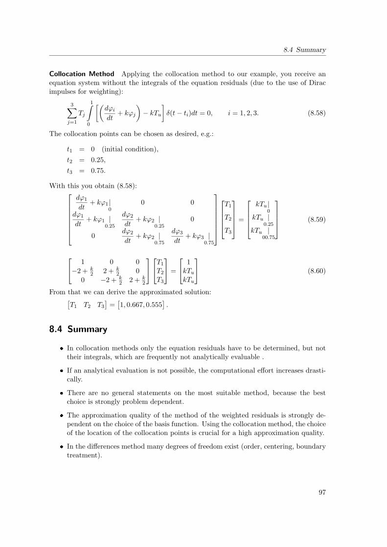
8.4 Summary
Collocation Method Applying the collocation method to our example, you receive anequation system without the integrals of the equation residuals (due to the use of Diracimpulses for weighting):
3∑j=1
Tj
1∫0
[(dϕi
dt+ kϕj
)− kTu
]δ(t− ti)dt = 0, i = 1, 2, 3. (8.58)
The collocation points can be chosen as desired, e.g.:
t1 = 0 (initial condition),t2 = 0.25,
t3 = 0.75.
With this you obtain (8.58):
dϕ1
dt+ kϕ1 |
00 0
dϕ1
dt+ kϕ1 |
0.25
dϕ2
dt+ kϕ2 |
0.250
0dϕ2
dt+ kϕ2 |
0.75
dϕ3
dt+ kϕ3 |
0.75
T1
T2
T3
=
kTu |
0
kTu |0.25
kTu |00.75
(8.59)
1 0 0−2 + k
2 2 + k2 0
0 −2 + k2 2 + k
2
T1
T2
T3
=
1kTu
kTu
(8.60)
From that we can derive the approximated solution:[T1 T2 T3
]=
[1, 0.667, 0.555
].
8.4 Summary
In collocation methods only the equation residuals have to be determined, but nottheir integrals, which are frequently not analytically evaluable .
If an analytical evaluation is not possible, the computational effort increases drasti-cally.
There are no general statements on the most suitable method, because the bestchoice is strongly problem dependent.
The approximation quality of the method of the weighted residuals is strongly de-pendent on the choice of the basis function. Using the collocation method, the choiceof the location of the collocation points is crucial for a high approximation quality.
In the differences method many degrees of freedom exist (order, centering, boundarytreatment).
97

8 Partial Differential Equations
98
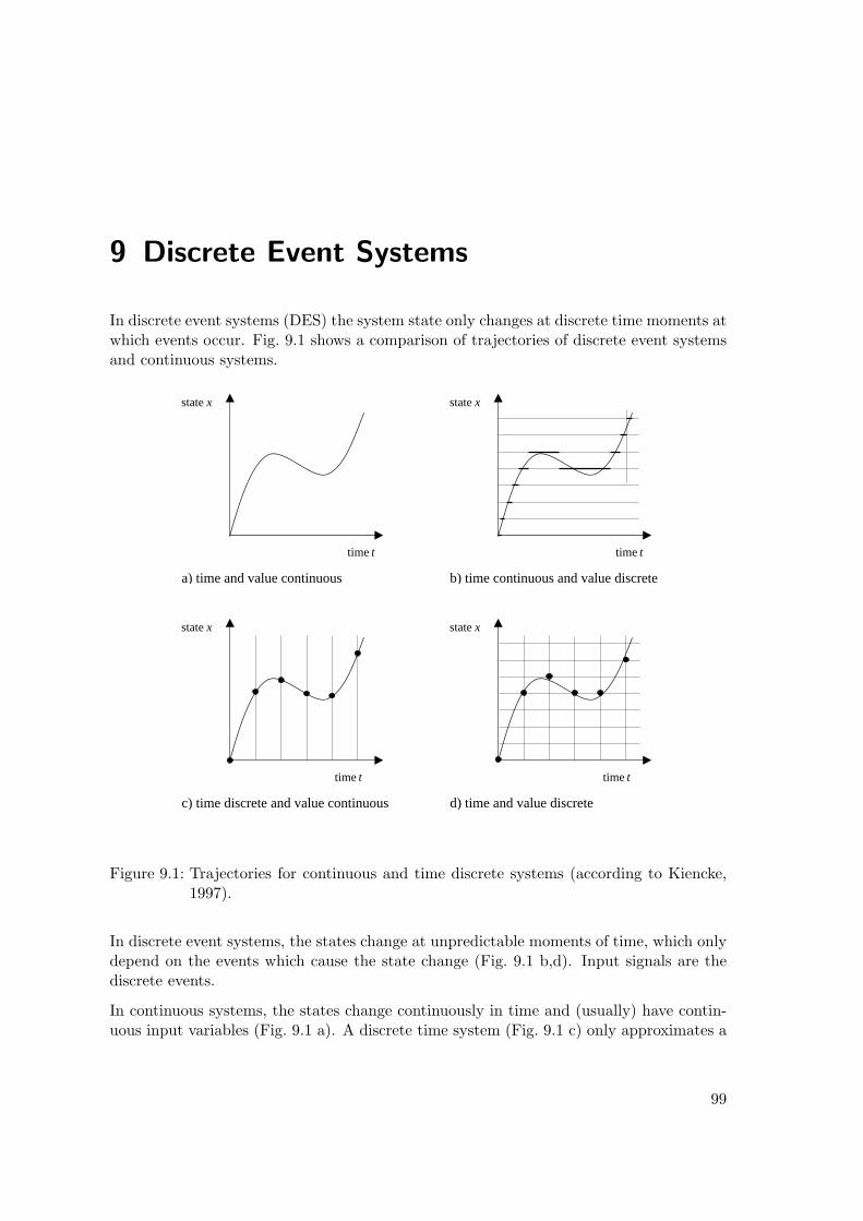
9 Discrete Event Systems
In discrete event systems (DES) the system state only changes at discrete time moments atwhich events occur. Fig. 9.1 shows a comparison of trajectories of discrete event systemsand continuous systems.
time t
state x
time t
state x
time t
state x
time t
state x
a) time and value continuous b) time continuous and value discrete
c) time discrete and value continuous d) time and value discrete
Figure 9.1: Trajectories for continuous and time discrete systems (according to Kiencke,1997).
In discrete event systems, the states change at unpredictable moments of time, which onlydepend on the events which cause the state change (Fig. 9.1 b,d). Input signals are thediscrete events.
In continuous systems, the states change continuously in time and (usually) have contin-uous input variables (Fig. 9.1 a). A discrete time system (Fig. 9.1 c) only approximates a
99
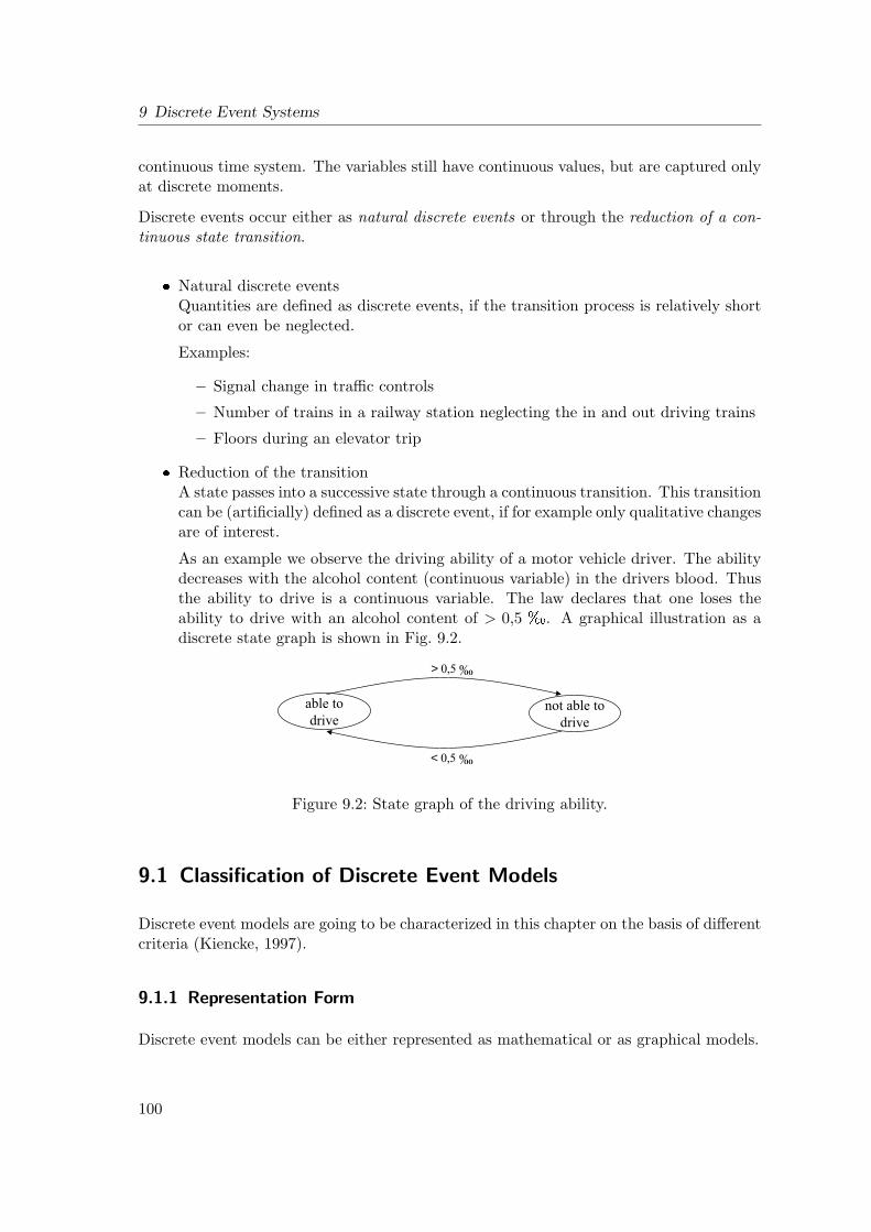
9 Discrete Event Systems
continuous time system. The variables still have continuous values, but are captured onlyat discrete moments.
Discrete events occur either as natural discrete events or through the reduction of a con-tinuous state transition.
Natural discrete eventsQuantities are defined as discrete events, if the transition process is relatively shortor can even be neglected.
Examples:
– Signal change in traffic controls
– Number of trains in a railway station neglecting the in and out driving trains
– Floors during an elevator trip
Reduction of the transitionA state passes into a successive state through a continuous transition. This transitioncan be (artificially) defined as a discrete event, if for example only qualitative changesare of interest.
As an example we observe the driving ability of a motor vehicle driver. The abilitydecreases with the alcohol content (continuous variable) in the drivers blood. Thusthe ability to drive is a continuous variable. The law declares that one loses theability to drive with an alcohol content of > 0,5 . A graphical illustration as adiscrete state graph is shown in Fig. 9.2.
<
>
Figure 9.2: State graph of the driving ability.
9.1 Classification of Discrete Event Models
Discrete event models are going to be characterized in this chapter on the basis of differentcriteria (Kiencke, 1997).
9.1.1 Representation Form
Discrete event models can be either represented as mathematical or as graphical models.
100
9.2 State Model
Mathematical modelThe objects are represented through mathematical variables as well as input andoutput functions. (see Section 9.2).
Graphical modelThe variables are depicted as graphical symbols. The input and output functionsare executed through graphical operations (see Section 9.3). The advantage of thisrepresentation is the vividness. On the other hand, graphical symbols often cannotcompletely represent a real process.
Every graphical model can be transformed into a mathematical model (e.g. withmatrix operations).
9.1.2 Time Basis
In opposite to time continuous models, no time basis is available in discrete time models.The model analysis is carried out for a logical sequence.
9.1.3 States and State Transitions
You distinguish between deterministic and stochastic states and state transitions. Stochas-tic states only appear with a specific probability. Thereby, the state transitions take placewith conditional probabilities.
9.2 State Model
A discrete event system is described with a model M , which can be represented by a7-tuple:
M = 〈x,z,y,ΦIN ,ΦEX ,Ω, τ〉 (9.1)
with
x = [x1, x2, . . . , xk]T vector of inputs (external events),
z = [z1, z2, . . . , zm]T vector of states ,
y = [y1, y2, . . . , yn]T vector of outputs.
mathematical
functions
ΦIN : z → z state transition function for internal eventsΦEX : z × x → z state transition function for external events
Ω : z × x → y output functionτ : z → R+ residence time function
101
9 Discrete Event Systems
State transition function for internal events
The system is in the state zi with its corresponding residence time τ(zi). A new state willbe reached after the end of the residence time:
z[t + τ(zi)] = ΦIN (zi) (9.2)
State transition function for external events
The system is in the state z(t). Because of an external event x(t) it switches to the newstate z′
z′(t) = ΦEX [z(t),x(t)] (9.3)
Output function
y(t) = Ω[z(t),x(t)] (9.4)
Input variables x
A model is called autonomous, if it works without being influenced by the environment(without inputs x).
M = 〈z,y,ΦIN ,Ω, τ〉
Time dependency
If the state transition functions ΦIN , ΦEX , the output function Ω, and the residencetime function τ are dependent on time, one calls the system time-variant, otherwise time-invariant.
Dependency of the the state transitions on the system’s previous history
A model is called “memoryless”, if the conditional transition probability for the successivestate is only dependent on the immediate state zi. This characteristic eases the mathe-matical analysis.
9.2.1 Example
We consider a liquid vessel as an illustrative example. The filling and emptying of thevessel is supposed to be realized by means of a digital feedforward control (see Fig. 9.3).
Three process states (filling, emptying, equilibrium) are considered in the model:
h > 0 if v1 6= 0, v2 = 0 (filling)
h < 0 if v1 = 0, v2 6= 0 (emptying)
h = 0 if v1 = v2
6= 0= 0
(equilibrium)
102
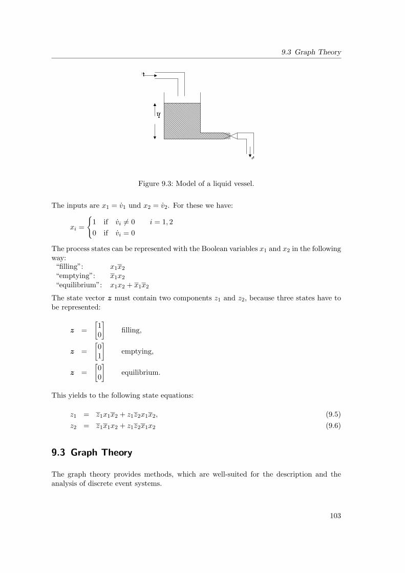
9.3 Graph Theory
Figure 9.3: Model of a liquid vessel.
The inputs are x1 = v1 und x2 = v2. For these we have:
xi =
1 if vi 6= 0 i = 1, 20 if vi = 0
The process states can be represented with the Boolean variables x1 and x2 in the followingway:“filling”: x1x2
“emptying”: x1x2
“equilibrium”: x1x2 + x1x2
The state vector z must contain two components z1 and z2, because three states have tobe represented:
z =[10
]filling,
z =[01
]emptying,
z =[00
]equilibrium.
This yields to the following state equations:
z1 = z1x1x2 + z1z2x1x2, (9.5)z2 = z1x1x2 + z1z2x1x2 (9.6)
9.3 Graph Theory
The graph theory provides methods, which are well-suited for the description and theanalysis of discrete event systems.
103
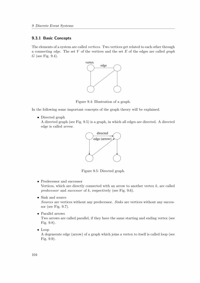
9 Discrete Event Systems
9.3.1 Basic Concepts
The elements of a system are called vertices. Two vertices get related to each other througha connecting edge. The set V of the vertices and the set E of the edges are called graphG (see Fig. 9.4).
Figure 9.4: Illustration of a graph.
In the following some important concepts of the graph theory will be explained.
Directed graphA directed graph (see Fig. 9.5) is a graph, in which all edges are directed. A directededge is called arrow.
Figure 9.5: Directed graph.
Predecessor and successorVertices, which are directly connected with an arrow to another vertex k, are calledpredecessor and successor of k, respectively (see Fig. 9.6).
Sink and sourceSources are vertices without any predecessor. Sinks are vertices without any succes-sor (see Fig. 9.7).
Parallel arrowsTwo arrows are called parallel, if they have the same starting and ending vertex (seeFig. 9.8).
LoopA degenerate edge (arrow) of a graph which joins a vertex to itself is called loop (seeFig. 9.9).
104
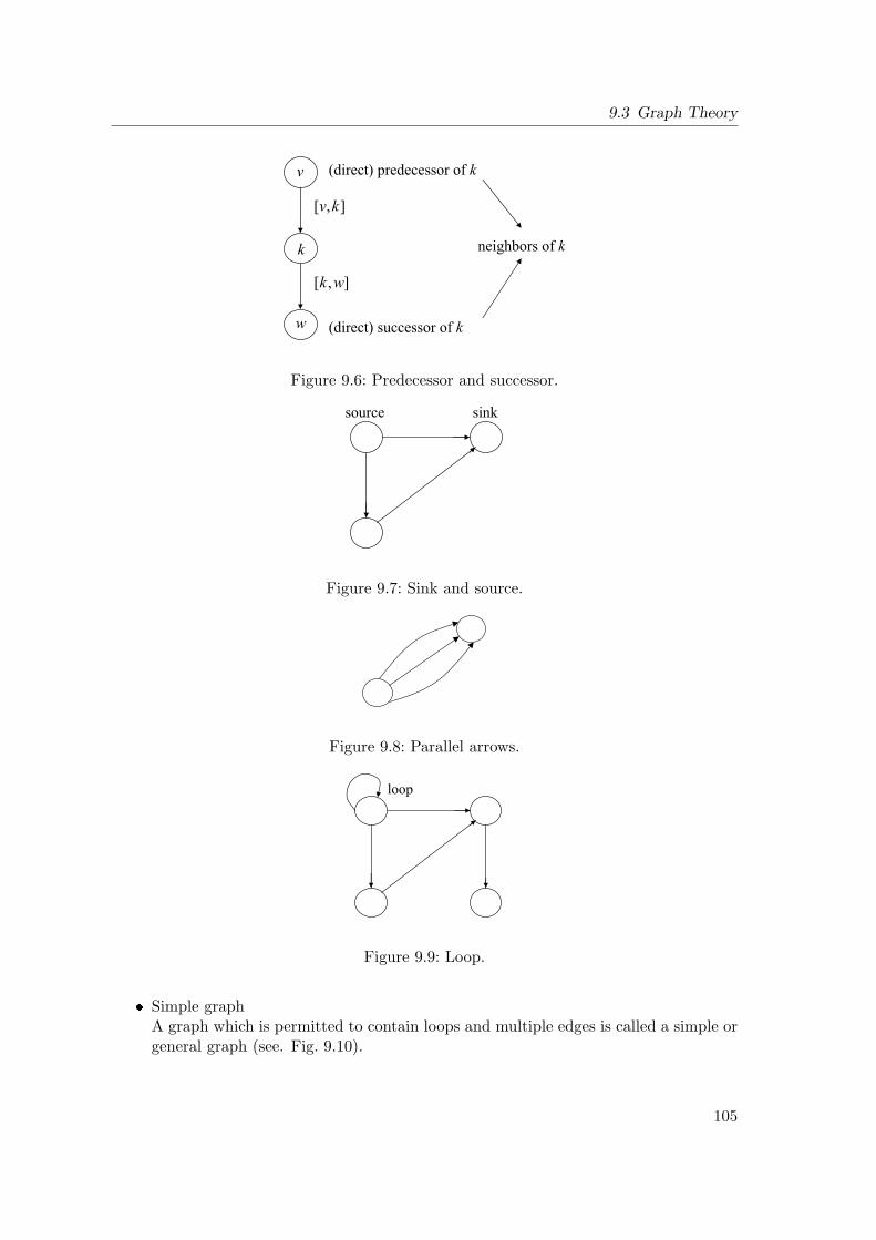
9.3 Graph Theory
Figure 9.6: Predecessor and successor.
Figure 9.7: Sink and source.
Figure 9.8: Parallel arrows.
Figure 9.9: Loop.
Simple graphA graph which is permitted to contain loops and multiple edges is called a simple orgeneral graph (see. Fig. 9.10).
105
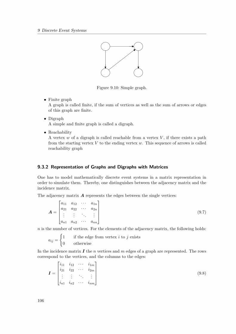
9 Discrete Event Systems
Figure 9.10: Simple graph.
Finite graphA graph is called finite, if the sum of vertices as well as the sum of arrows or edgesof this graph are finite.
DigraphA simple and finite graph is called a digraph.
ReachabilityA vertex w of a digraph is called reachable from a vertex V , if there exists a pathfrom the starting vertex V to the ending vertex w. This sequence of arrows is calledreachability graph
9.3.2 Representation of Graphs and Digraphs with Matrices
One has to model mathematically discrete event systems in a matrix representation inorder to simulate them. Thereby, one distinguishes between the adjacency matrix and theincidence matrix.
The adjacency matrix A represents the edges between the single vertices:
A =
a11 a12 · · · a1n
a21 a22 · · · a2n...
.... . .
...an1 an2 · · · ann
(9.7)
n is the number of vertices. For the elements of the adjacency matrix, the following holds:
aij =
1 if the edge from vertex i to j exists0 otherwise
In the incidence matrix I the n vertices and m edges of a graph are represented. The rowscorrespond to the vertices, and the columns to the edges:
I =
i11 i12 · · · i1m
i21 i22 · · · i2m...
.... . .
...in1 in2 · · · inm
(9.8)
106
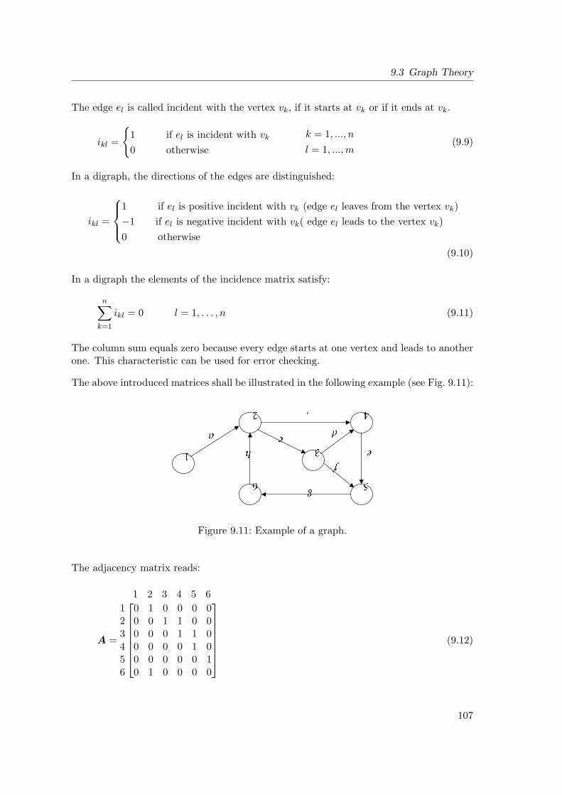
9.3 Graph Theory
The edge el is called incident with the vertex vk, if it starts at vk or if it ends at vk.
ikl =
1 if el is incident with vk
0 otherwise
k = 1, ..., n
l = 1, ...,m(9.9)
In a digraph, the directions of the edges are distinguished:
ikl =
1 if el is positive incident with vk (edge el leaves from the vertex vk)−1 if el is negative incident with vk( edge el leads to the vertex vk)0 otherwise
(9.10)
In a digraph the elements of the incidence matrix satisfy:
n∑k=1
ikl = 0 l = 1, . . . , n (9.11)
The column sum equals zero because every edge starts at one vertex and leads to anotherone. This characteristic can be used for error checking.
The above introduced matrices shall be illustrated in the following example (see Fig. 9.11):
Figure 9.11: Example of a graph.
The adjacency matrix reads:
A =
1 2 3 4 5 6123456
0 1 0 0 0 00 0 1 1 0 00 0 0 1 1 00 0 0 0 1 00 0 0 0 0 10 1 0 0 0 0
(9.12)
107
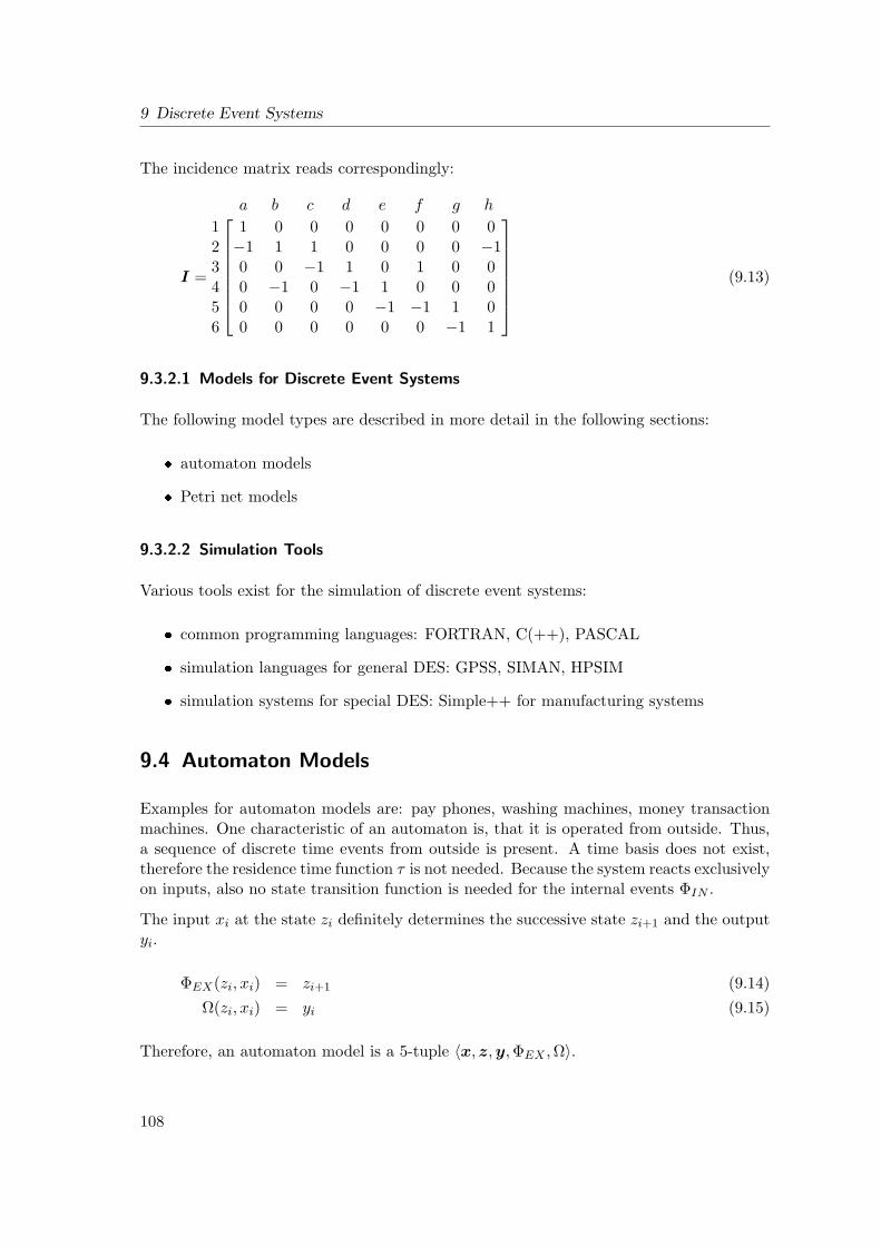
9 Discrete Event Systems
The incidence matrix reads correspondingly:
I =
a b c d e f g h
123456
1 0 0 0 0 0 0 0−1 1 1 0 0 0 0 −10 0 −1 1 0 1 0 00 −1 0 −1 1 0 0 00 0 0 0 −1 −1 1 00 0 0 0 0 0 −1 1
(9.13)
9.3.2.1 Models for Discrete Event Systems
The following model types are described in more detail in the following sections:
automaton models
Petri net models
9.3.2.2 Simulation Tools
Various tools exist for the simulation of discrete event systems:
common programming languages: FORTRAN, C(++), PASCAL
simulation languages for general DES: GPSS, SIMAN, HPSIM
simulation systems for special DES: Simple++ for manufacturing systems
9.4 Automaton Models
Examples for automaton models are: pay phones, washing machines, money transactionmachines. One characteristic of an automaton is, that it is operated from outside. Thus,a sequence of discrete time events from outside is present. A time basis does not exist,therefore the residence time function τ is not needed. Because the system reacts exclusivelyon inputs, also no state transition function is needed for the internal events ΦIN .
The input xi at the state zi definitely determines the successive state zi+1 and the outputyi.
ΦEX(zi, xi) = zi+1 (9.14)Ω(zi, xi) = yi (9.15)
Therefore, an automaton model is a 5-tuple 〈x,z,y,ΦEX ,Ω〉.
108
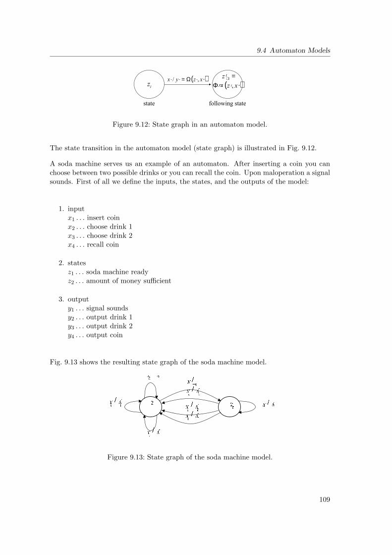
9.4 Automaton Models
( ) Ω=( )Φ
=+
Figure 9.12: State graph in an automaton model.
The state transition in the automaton model (state graph) is illustrated in Fig. 9.12.
A soda machine serves us an example of an automaton. After inserting a coin you canchoose between two possible drinks or you can recall the coin. Upon maloperation a signalsounds. First of all we define the inputs, the states, and the outputs of the model:
1. inputx1 . . . insert coinx2 . . . choose drink 1x3 . . . choose drink 2x4 . . . recall coin
2. statesz1 . . . soda machine readyz2 . . . amount of money sufficient
3. outputy1 . . . signal soundsy2 . . . output drink 1y3 . . . output drink 2y4 . . . output coin
Fig. 9.13 shows the resulting state graph of the soda machine model.
−
!"# $%
&'( )*
Figure 9.13: State graph of the soda machine model.
109
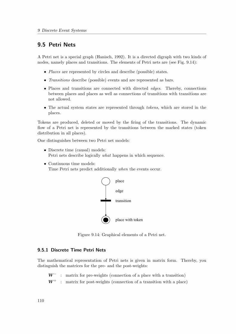
9 Discrete Event Systems
9.5 Petri Nets
A Petri net is a special graph (Hanisch, 1992). It is a directed digraph with two kinds ofnodes, namely places and transitions. The elements of Petri nets are (see Fig. 9.14):
Places are represented by circles and describe (possible) states.
Transitions describe (possible) events and are represented as bars.
Places and transitions are connected with directed edges. Thereby, connectionsbetween places and places as well as connections of transitions with transitions arenot allowed.
The actual system states are represented through tokens, which are stored in theplaces.
Tokens are produced, deleted or moved by the firing of the transitions. The dynamicflow of a Petri net is represented by the transitions between the marked states (tokendistribution in all places).
One distinguishes between two Petri net models:
Discrete time (causal) models:Petri nets describe logically what happens in which sequence.
Continuous time models:Time Petri nets predict additionally when the events occur.
Figure 9.14: Graphical elements of a Petri net.
9.5.1 Discrete Time Petri Nets
The mathematical representation of Petri nets is given in matrix form. Thereby, youdistinguish the matrices for the pre- and the post-weights:
W− : matrix for pre-weights (connection of a place with a transition)W + : matrix for post-weights (connection of a transition with a place)
110
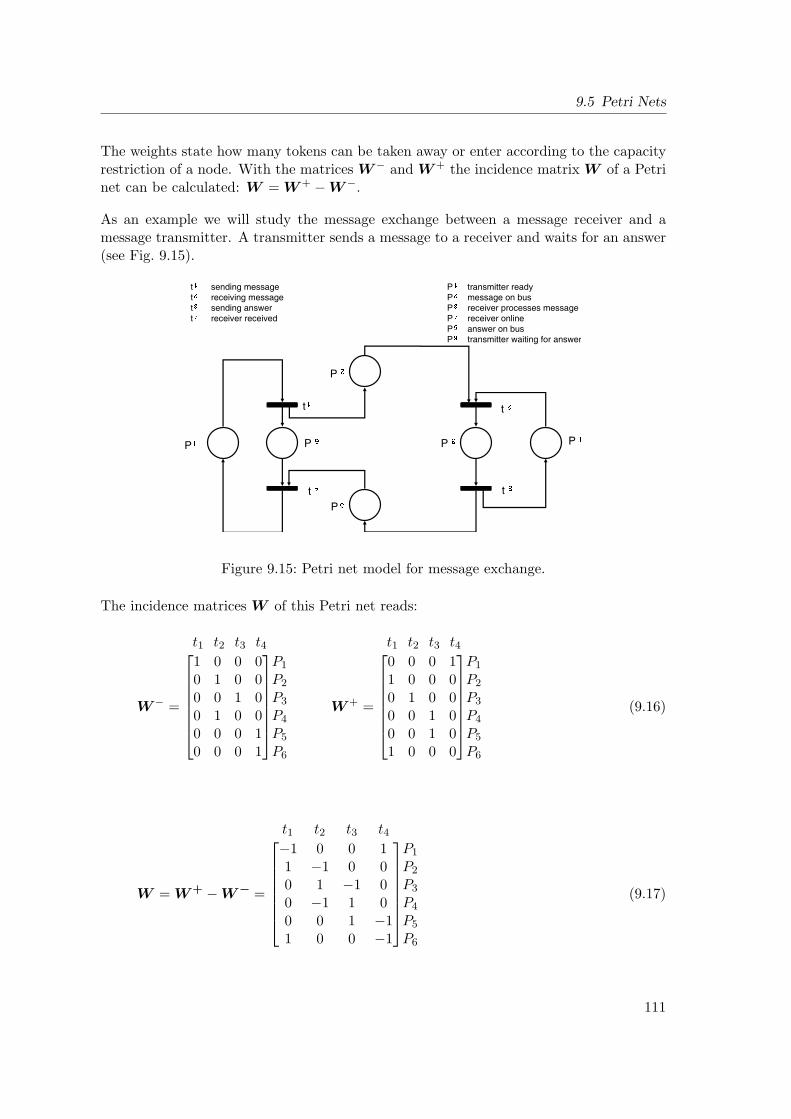
9.5 Petri Nets
The weights state how many tokens can be taken away or enter according to the capacityrestriction of a node. With the matrices W− and W + the incidence matrix W of a Petrinet can be calculated: W = W + −W−.
As an example we will study the message exchange between a message receiver and amessage transmitter. A transmitter sends a message to a receiver and waits for an answer(see Fig. 9.15).
Figure 9.15: Petri net model for message exchange.
The incidence matrices W of this Petri net reads:
W− =
t1 t2 t3 t4
1 0 0 00 1 0 00 0 1 00 1 0 00 0 0 10 0 0 1
P1
P2
P3
P4
P5
P6
W + =
t1 t2 t3 t4
0 0 0 11 0 0 00 1 0 00 0 1 00 0 1 01 0 0 0
P1
P2
P3
P4
P5
P6
(9.16)
W = W + −W − =
t1 t2 t3 t4
−1 0 0 11 −1 0 00 1 −1 00 −1 1 00 0 1 −11 0 0 −1
P1
P2
P3
P4
P5
P6
(9.17)
111
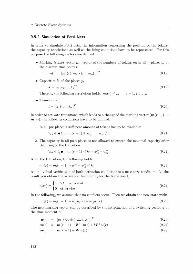
9 Discrete Event Systems
9.5.2 Simulation of Petri Nets
In order to simulate Petri nets, the information concerning the position of the tokens,the capacity restrictions as well as the firing conditions have to be represented. For thispurpose the following vectors are defined:
Marking (state) vector m: vector of the numbers of tokens mi in all n places pi atthe discrete time point r
m(r) = [m1(r),m2(r), ...,mn(r)]T (9.18)
Capacities ki of the places pi
k = [k1, k2, ..., kn]T (9.19)
Thereby, the following restriction holds: mi(r) ≤ ki i = 1, 2, . . . , n
Transitions
t = [t1, t2, ..., tm]T (9.20)
In order to activate transitions, which leads to a change of the marking vector (m(r−1) →m(r)), the following conditions have to be fulfilled:
1. In all pre-places a sufficient amount of tokens has to be available:
∀pi ∈ utj : mi(r − 1) ≥ w−ij w−ij 6= 0 (9.21)
2. The capacity in all post-places is not allowed to exceed the maximal capacity afterthe firing of the transition:
∀pi ∈ tj u : mi(r − 1) ≤ ki + w−ij − w+ij (9.22)
After the transition, the following holds:
mi(r) = mi(r − 1)− w−ij + w+ij ≤ ki (9.23)
An individual verification of both activation conditions is a necessary condition. As theresult you obtain the activation function uj for the transition tj :
uj(r) =
1 ∀ tj activated0 otherwise
(9.24)
In the following, we assume that no conflicts occur. Then we obtain the new state with:
mi(r) = mi(r − 1)− w−ijuj(r) + w+ijuj(r) (9.25)
The new marking vector can be described by the introduction of a switching vector u atthe time moment r:
u(r) = [u1(r), u2(r), ..., um(r)]T (9.26)m(r) = m(r − 1)−W− u(r) + W + u(r) (9.27)m(r) = m(r − 1) + W u(r) (9.28)
112
9.5 Petri Nets
9.5.3 Characteristics of Petri Nets
One advantage of Petri nets lies in the fact that many characteristics of control systemscan be analyzed with the help of Petri nets. Therefore, we want to explain the mostimportant characteristics of Petri nets in the following section.
9.5.3.1 Reachability
A state Ml is called reachable for a starting state M0, if there is a firing sequence, whichtransports M0 into Ml. This reachability graph is the basis for many analysis methods.In the example of the message exchange the reachability graph is given in Fig. 9.16.
( ) [ ]
= ( ) [ ]
=
( ) [ ]
=( ) [ ] !"
=#
$%
&'
()
*+
Figure 9.16: Reachability graph for the message exchange model.
One sees clearly that all states can be reached from any starting state. One uses thereachability graph for instance to review, whether desired states are not and undesiredstates are reachable. In this case the Petri net design has to be improved. Furthermore,one can avoid predecessors of dangerous states by the use of suitable design methods.
9.5.3.2 Boundedness and Safety
A Petri net is said to be bounded if in no single place pi more than a certain maximalamount of ki tokens are present. In the case of ki = 1 the Petri net is also said to be safe.
9.5.3.3 Deadlock
A deadlock in a Petri net is a transition (or a set of transitions) which cannot fire. Weconsider again the slightly modified example of the messages exchange (see Fig. 9.17).Through the introduction of the new transitions t5 and t6 deadlocks appear.
113
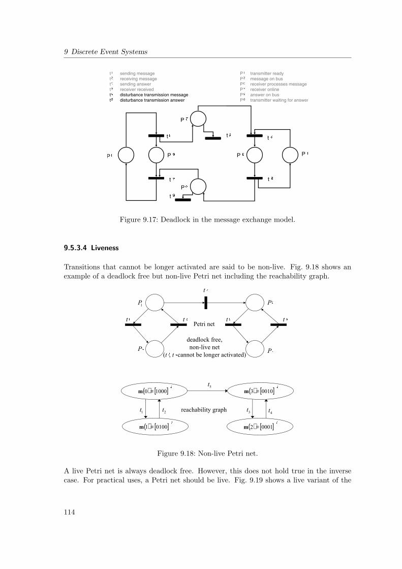
9 Discrete Event Systems
Figure 9.17: Deadlock in the message exchange model.
9.5.3.4 Liveness
Transitions that cannot be longer activated are said to be non-live. Fig. 9.18 shows anexample of a deadlock free but non-live Petri net including the reachability graph.
( ) [ ]
= ( ) [ ]
=
( ) [ ]
=( ) [ ]
=
Figure 9.18: Non-live Petri net.
A live Petri net is always deadlock free. However, this does not hold true in the inversecase. For practical uses, a Petri net should be live. Fig. 9.19 shows a live variant of the
114
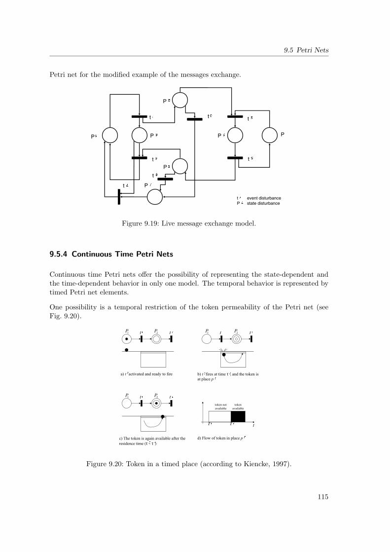
9.5 Petri Nets
Petri net for the modified example of the messages exchange.
Figure 9.19: Live message exchange model.
9.5.4 Continuous Time Petri Nets
Continuous time Petri nets offer the possibility of representing the state-dependent andthe time-dependent behavior in only one model. The temporal behavior is represented bytimed Petri net elements.
One possibility is a temporal restriction of the token permeability of the Petri net (seeFig. 9.20).
τ
τ τ
ττ
Figure 9.20: Token in a timed place (according to Kiencke, 1997).
115
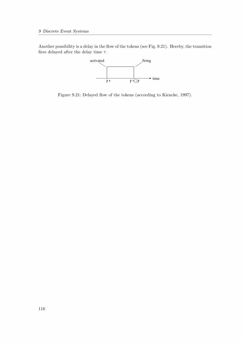
9 Discrete Event Systems
Another possibility is a delay in the flow of the tokens (see Fig. 9.21). Hereby, the transitionfires delayed after the delay time τ .
τ ττ +
Figure 9.21: Delayed flow of the tokens (according to Kiencke, 1997).
116
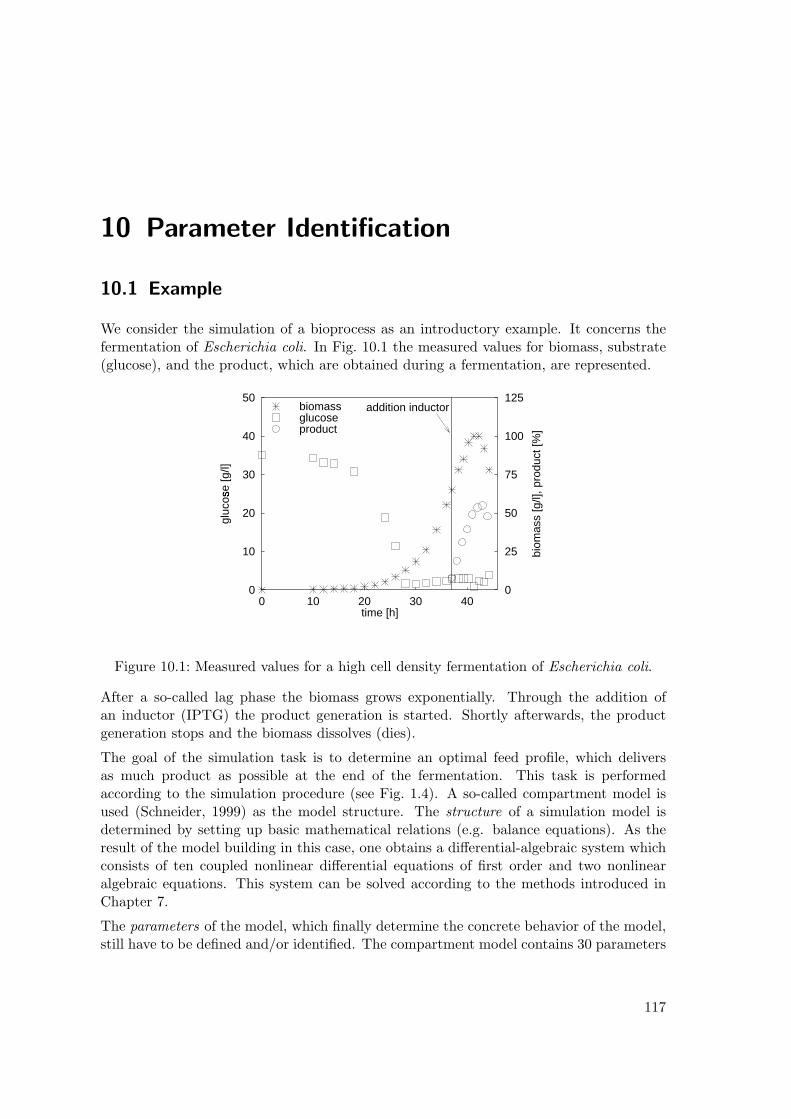
10 Parameter Identification
10.1 Example
We consider the simulation of a bioprocess as an introductory example. It concerns thefermentation of Escherichia coli. In Fig. 10.1 the measured values for biomass, substrate(glucose), and the product, which are obtained during a fermentation, are represented.
0
10
20
30
40
50
0 10 20 30 400
25
50
75
100
125
gluc
ose
[g/l]
biom
ass
[g/l]
, pro
duct
[%]
time [h]
addition inductorbiomassglucoseproduct
Figure 10.1: Measured values for a high cell density fermentation of Escherichia coli.
After a so-called lag phase the biomass grows exponentially. Through the addition ofan inductor (IPTG) the product generation is started. Shortly afterwards, the productgeneration stops and the biomass dissolves (dies).
The goal of the simulation task is to determine an optimal feed profile, which deliversas much product as possible at the end of the fermentation. This task is performedaccording to the simulation procedure (see Fig. 1.4). A so-called compartment model isused (Schneider, 1999) as the model structure. The structure of a simulation model isdetermined by setting up basic mathematical relations (e.g. balance equations). As theresult of the model building in this case, one obtains a differential-algebraic system whichconsists of ten coupled nonlinear differential equations of first order and two nonlinearalgebraic equations. This system can be solved according to the methods introduced inChapter 7.
The parameters of the model, which finally determine the concrete behavior of the model,still have to be defined and/or identified. The compartment model contains 30 parameters
117
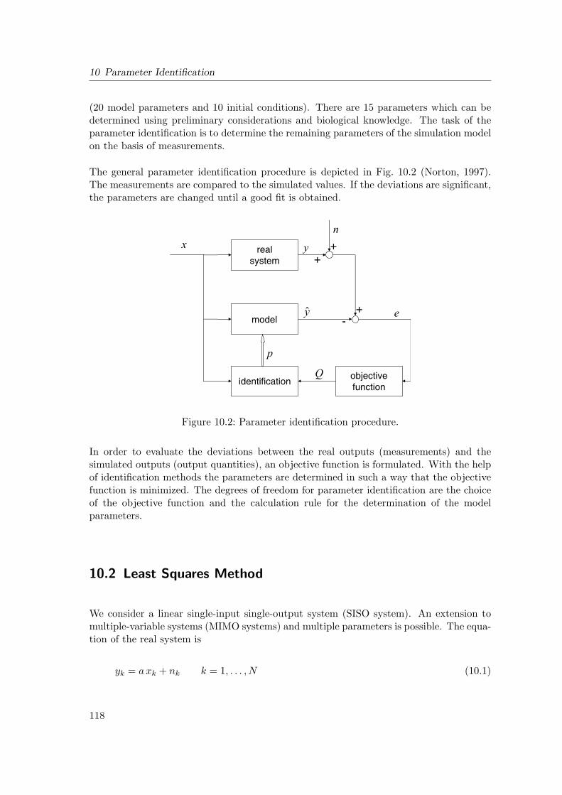
10 Parameter Identification
(20 model parameters and 10 initial conditions). There are 15 parameters which can bedetermined using preliminary considerations and biological knowledge. The task of theparameter identification is to determine the remaining parameters of the simulation modelon the basis of measurements.
The general parameter identification procedure is depicted in Fig. 10.2 (Norton, 1997).The measurements are compared to the simulated values. If the deviations are significant,the parameters are changed until a good fit is obtained.
Figure 10.2: Parameter identification procedure.
In order to evaluate the deviations between the real outputs (measurements) and thesimulated outputs (output quantities), an objective function is formulated. With the helpof identification methods the parameters are determined in such a way that the objectivefunction is minimized. The degrees of freedom for parameter identification are the choiceof the objective function and the calculation rule for the determination of the modelparameters.
10.2 Least Squares Method
We consider a linear single-input single-output system (SISO system). An extension tomultiple-variable systems (MIMO systems) and multiple parameters is possible. The equa-tion of the real system is
yk = a xk + nk k = 1, . . . , N (10.1)
118
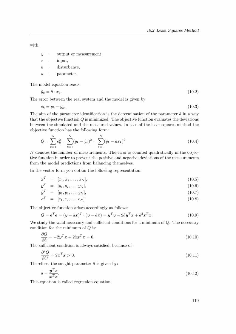
10.2 Least Squares Method
with
y : output or measurement,x : input,n : disturbance,a : parameter.
The model equation reads:
yk = a · xk. (10.2)
The error between the real system and the model is given by
ek = yk − yk. (10.3)
The aim of the parameter identification is the determination of the parameter a in a waythat the objective function Q is minimized. The objective function evaluates the deviationsbetween the simulated and the measured values. In case of the least squares method theobjective function has the following form:
Q =N∑
k=1
e2k =
N∑k=1
(yk − yk)2 =N∑
k=1
(yk − axk)2 (10.4)
N denotes the number of measurements. The error is counted quadratically in the objec-tive function in order to prevent the positive and negative deviations of the measurementsfrom the model predictions from balancing themselves.
In the vector form you obtain the following representation:
xT = [x1, x2, . . . , xN ], (10.5)yT = [y1, y2, . . . , yN ], (10.6)yT = [y1, y2, . . . , yN ], (10.7)eT = [e1, e2, . . . , eN ]. (10.8)
The objective function arises accordingly as follows:
Q = eT e = (y − ax)T · (y − ax) = yT y − 2ayT x + a2xT x. (10.9)
We study the valid necessary and sufficient conditions for a minimum of Q. The necessarycondition for the minimum of Q is:
∂Q
∂a= −2yT x + 2axT x = 0. (10.10)
The sufficient condition is always satisfied, because of
∂2Q
∂a2= 2xT x > 0. (10.11)
Therefore, the sought parameter a is given by:
a =yT x
xT x. (10.12)
This equation is called regression equation.
119
10 Parameter Identification
10.3 Method of Weighted Least Squares
The method of least squares does not use any information about the disturbance n. Ifsuch information exists, it can be used for an improvement of the result of the parameteridentification. The idea of the method of weighted least squares consists of weighting theerrors e with factors λk:
Q =N∑
k=1
1λk
e2k = eTΛ−1e. (10.13)
Λ is a weighting matrix. Information about the disturbance can be available e.g. in formof the variance matrix C. Therefore, this variance matrix is a sensible choice for Λ.
Λ = C. (10.14)
The variance matrix has the following form:
C =
σ2(n1) 0 · · · 0
0 σ2(n2) · · · 0...
.... . .
...0 0 · · · σ2(nN )
. (10.15)
With this you obtain as the objective function
Q = (y − ax)T C−1(y − ax) = yT C−1y − 2ayT C−1x + a2xT C−1x (10.16)
The necessary condition for the minimum of the objective function leads to:
∂Q
∂a= −2yT C−1x + 2axT C−1x = 0. (10.17)
The sought parameter a arises as follows:
a =yT C−1x
xT C−1x. (10.18)
This identification method is called Markov estimation, if Λ is the covariance matrix ofthe disturbance.
In many cases the expectation E can be characterized by
E[n(ti)] = E[n] = 0, (10.19)E[nin
Tj ] = δijC(ti). (10.20)
This leads to a simplification of the objective function
Q =1σ2
eT e. (10.21)
120
10.4 Multiple Inputs and Parameters
10.4 Multiple Inputs and Parameters
The introduced methods can be extended for the case of m inputs x and parameters a.With one output and N measurements the following equation is obtained:
yk = a1x1k + a2x
2k + · · ·+ amxm
k + nk k = 1, . . . , N. (10.22)
In vector form the equations are:
y = Xa + n or
y1
y2...
yN
=
x1
1 x21 · · · xm
1
x12 · · · · · · xm
2...
.... . .
...x1
N x2N · · · xm
N
a1
a2...
am
+
n1
n2...
nN
. (10.23)
The model equations read:
y = X · a. (10.24)
Correspondingly, the objective function is:
Q = eT e = (y − y)T · (y − y) = (y −Xa)T · (y −Xa)
= yT y − aT XT y − yT Xa + aT XT Xa.(10.25)
The necessary condition
∂Q
∂a= −2XT y + 2XT Xa = 0 (10.26)
leads to the normal equation
XT Xa = XT y, (10.27)
with which the sought parameters a can be calculated:
a = (XT X)−1XT y. (10.28)
If (XT X)−1 is ill-conditioned, you will have numerical problems inverting the matrix.
10.5 Recursive Regression
If one wants to (quickly) carry out online parameter identifications, the method of recursiveregression is applied. In this method, the parameter ak+1 is estimated on the basis of eachnew measured value yk+1 using previously calculated quantities. This possibility arises, ifthe parameter estimation can be carried out in parallel with consecutive measuring (e.g.for adaptive control). The goal is the determination of new estimates with the help of theold ones and the updated measurements.
121
10 Parameter Identification
The k-th estimation (up to the present k measurements are available) is given as (see(10.28)):
ak = (XTk Xk)−1XT
k yk. (10.29)
The (k + 1)-th estimation is:
ak+1 = (XTk+1Xk+1)−1XT
k+1yk+1. (10.30)
With
XTk+1yk+1 =
x1
1 x21 · · · x1
k | x1k+1
x12 x2
2 · · · x1k | x2
k+1...
.... . .
... |...
xm1 xm
2 · · · xmk | xm
k+1
·
y1
y2...
yk
—yk+1
= XT
k yk + xk+1yk+1 (10.31)
you obtain
ak+1 = (XTk+1Xk+1)−1(XT
k yk + xk+1yk+1). (10.32)
(10.29) can be transformed to
XTk Xkak = XT
k yk. (10.33)
This equation is inserted into (10.32):
ak+1 = (XTk+1Xk+1)−1Xk
T Xkak + (XTk+1Xk+1)−1xk+1yk+1 +ak − ak︸ ︷︷ ︸
extension
. (10.34)
We now define the matrix Sk as
Sk = (XTk Xk)−1 (10.35)
and obtain
ak+1 = ak +((
Sk+1S−1k
)− I
)ak + Sk+1xk+1yk+1. (10.36)
Sk+1 reads
Sk+1 = (XTk Xk + xk+1x
Tk+1)
−1 = (S−1k + xk+1x
Tk+1)
−1, (10.37)
therefore S−1k can be written as
S−1k = S−1
k+1 − xk+1xTk+1. (10.38)
The estimation equation of the recursive regression is
ak+1 = ak + Sk+1xk+1 (yk+1 − xTk+1ak)︸ ︷︷ ︸
error
, a0 = 0, (10.39)
with Sk+1 (because of the matrix inversion lemma):
Sk+1 = Sk −1
1 + xTk+1Skxk+1
Skxk+1xTk+1Sk, S0 = I. (10.40)
122
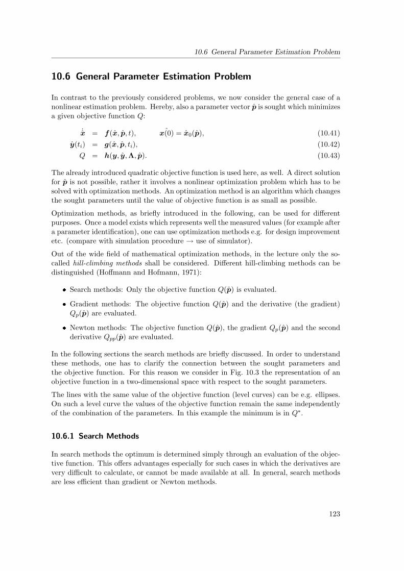
10.6 General Parameter Estimation Problem
10.6 General Parameter Estimation Problem
In contrast to the previously considered problems, we now consider the general case of anonlinear estimation problem. Hereby, also a parameter vector p is sought which minimizesa given objective function Q:
˙x = f(x, p, t), ˆx(0) = x0(p), (10.41)y(ti) = g(x, p, ti), (10.42)
Q = h(y, y,Λ, p). (10.43)
The already introduced quadratic objective function is used here, as well. A direct solutionfor p is not possible, rather it involves a nonlinear optimization problem which has to besolved with optimization methods. An optimization method is an algorithm which changesthe sought parameters until the value of objective function is as small as possible.
Optimization methods, as briefly introduced in the following, can be used for differentpurposes. Once a model exists which represents well the measured values (for example aftera parameter identification), one can use optimization methods e.g. for design improvementetc. (compare with simulation procedure → use of simulator).
Out of the wide field of mathematical optimization methods, in the lecture only the so-called hill-climbing methods shall be considered. Different hill-climbing methods can bedistinguished (Hoffmann and Hofmann, 1971):
Search methods: Only the objective function Q(p) is evaluated.
Gradient methods: The objective function Q(p) and the derivative (the gradient)Qp(p) are evaluated.
Newton methods: The objective function Q(p), the gradient Qp(p) and the secondderivative Qpp(p) are evaluated.
In the following sections the search methods are briefly discussed. In order to understandthese methods, one has to clarify the connection between the sought parameters andthe objective function. For this reason we consider in Fig. 10.3 the representation of anobjective function in a two-dimensional space with respect to the sought parameters.
The lines with the same value of the objective function (level curves) can be e.g. ellipses.On such a level curve the values of the objective function remain the same independentlyof the combination of the parameters. In this example the minimum is in Q∗.
10.6.1 Search Methods
In search methods the optimum is determined simply through an evaluation of the objec-tive function. This offers advantages especially for such cases in which the derivatives arevery difficult to calculate, or cannot be made available at all. In general, search methodsare less efficient than gradient or Newton methods.
123
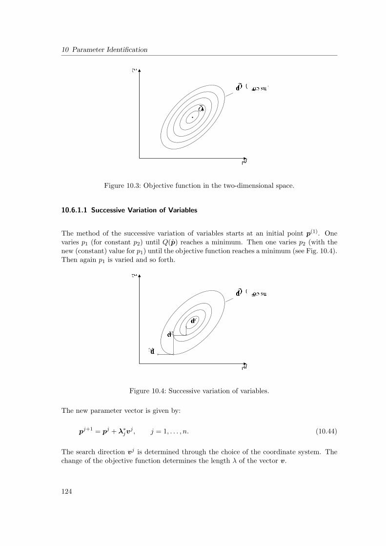
10 Parameter Identification
Figure 10.3: Objective function in the two-dimensional space.
10.6.1.1 Successive Variation of Variables
The method of the successive variation of variables starts at an initial point p(1). Onevaries p1 (for constant p2) until Q(p) reaches a minimum. Then one varies p2 (with thenew (constant) value for p1) until the objective function reaches a minimum (see Fig. 10.4).Then again p1 is varied and so forth.
Figure 10.4: Successive variation of variables.
The new parameter vector is given by:
pj+1 = pj + λ∗jvj , j = 1, . . . , n. (10.44)
The search direction vj is determined through the choice of the coordinate system. Thechange of the objective function determines the length λ of the vector v.
124
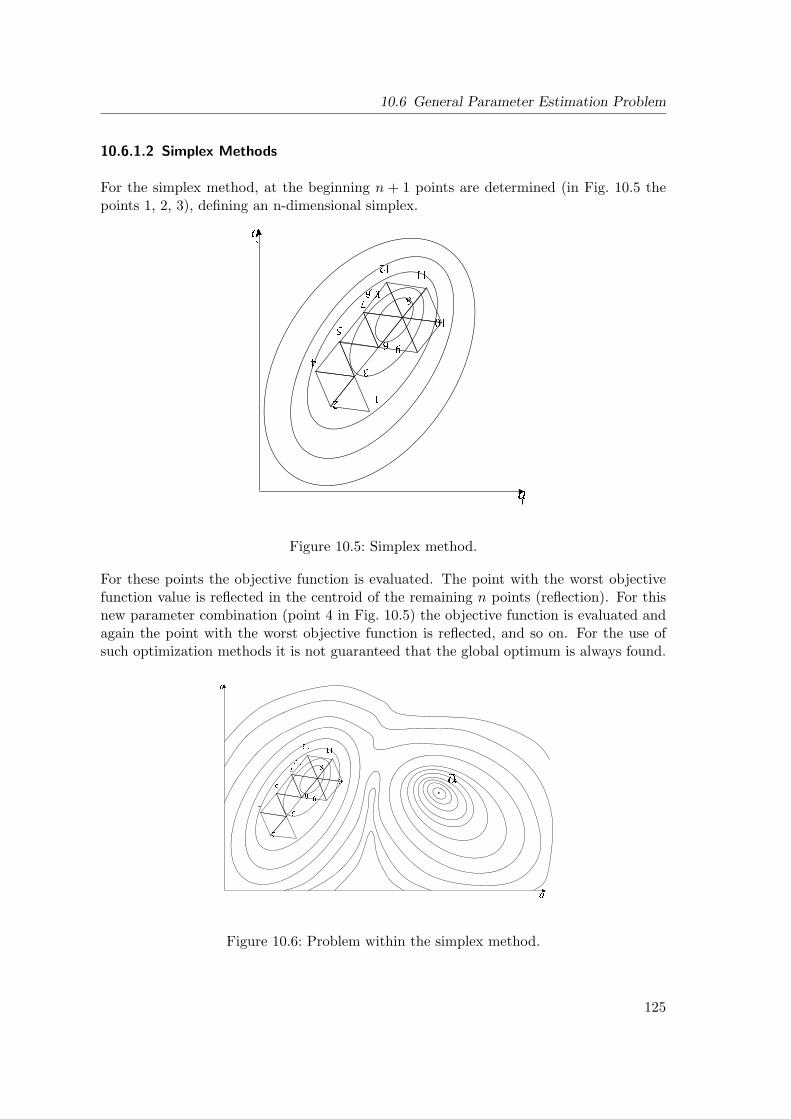
10.6 General Parameter Estimation Problem
10.6.1.2 Simplex Methods
For the simplex method, at the beginning n + 1 points are determined (in Fig. 10.5 thepoints 1, 2, 3), defining an n-dimensional simplex.
Figure 10.5: Simplex method.
For these points the objective function is evaluated. The point with the worst objectivefunction value is reflected in the centroid of the remaining n points (reflection). For thisnew parameter combination (point 4 in Fig. 10.5) the objective function is evaluated andagain the point with the worst objective function is reflected, and so on. For the use ofsuch optimization methods it is not guaranteed that the global optimum is always found.
Figure 10.6: Problem within the simplex method.
125
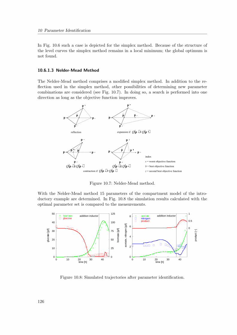
10 Parameter Identification
In Fig. 10.6 such a case is depicted for the simplex method. Because of the structure ofthe level curves the simplex method remains in a local minimum; the global optimum isnot found.
10.6.1.3 Nelder-Mead Method
The Nelder-Mead method comprises a modified simplex method. In addition to the re-flection used in the simplex method, other possibilities of determining new parametercombinations are considered (see Fig. 10.7). In doing so, a search is performed into onedirection as long as the objective function improves.
( ) ( ) <
( ) ( ) ≥ ( ) ( ) ≤( ) ( ) >
Figure 10.7: Nelder-Mead method.
With the Nelder-Mead method 15 parameters of the compartment model of the intro-ductory example are determined. In Fig. 10.8 the simulation results calculated with theoptimal parameter set is compared to the measurements.
0
10
20
30
40
50
0 10 20 30 400
25
50
75
100
125
gluc
ose
[g/l]
biom
ass
[g/l]
time [h]
addition inductorbiomassglucose
0
2
4
6
8
0 10 20 30 40
0
0.5
1
acet
ate,
nitr
ogen
[g/l]
prod
uct [
−]
time [h]
addition inductoracetatenitrogenproduct
Figure 10.8: Simulated trajectories after parameter identification.
126
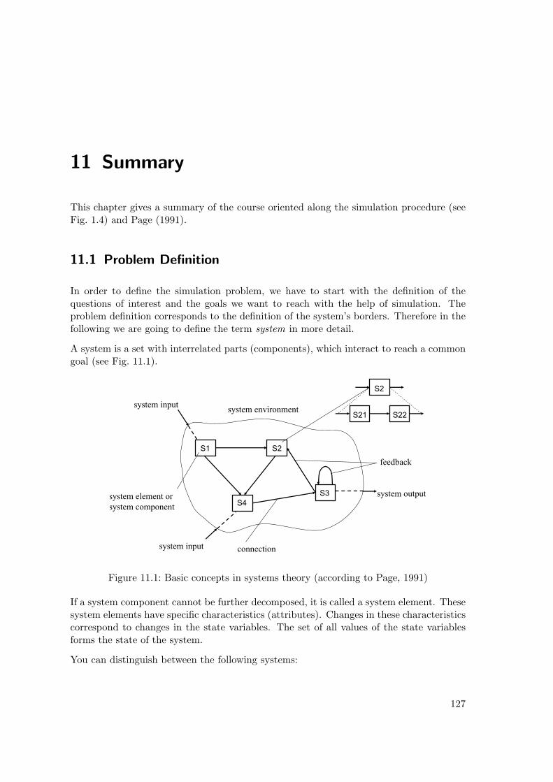
11 Summary
This chapter gives a summary of the course oriented along the simulation procedure (seeFig. 1.4) and Page (1991).
11.1 Problem Definition
In order to define the simulation problem, we have to start with the definition of thequestions of interest and the goals we want to reach with the help of simulation. Theproblem definition corresponds to the definition of the system’s borders. Therefore in thefollowing we are going to define the term system in more detail.
A system is a set with interrelated parts (components), which interact to reach a commongoal (see Fig. 11.1).
Figure 11.1: Basic concepts in systems theory (according to Page, 1991)
If a system component cannot be further decomposed, it is called a system element. Thesesystem elements have specific characteristics (attributes). Changes in these characteristicscorrespond to changes in the state variables. The set of all values of the state variablesforms the state of the system.
You can distinguish between the following systems:
127
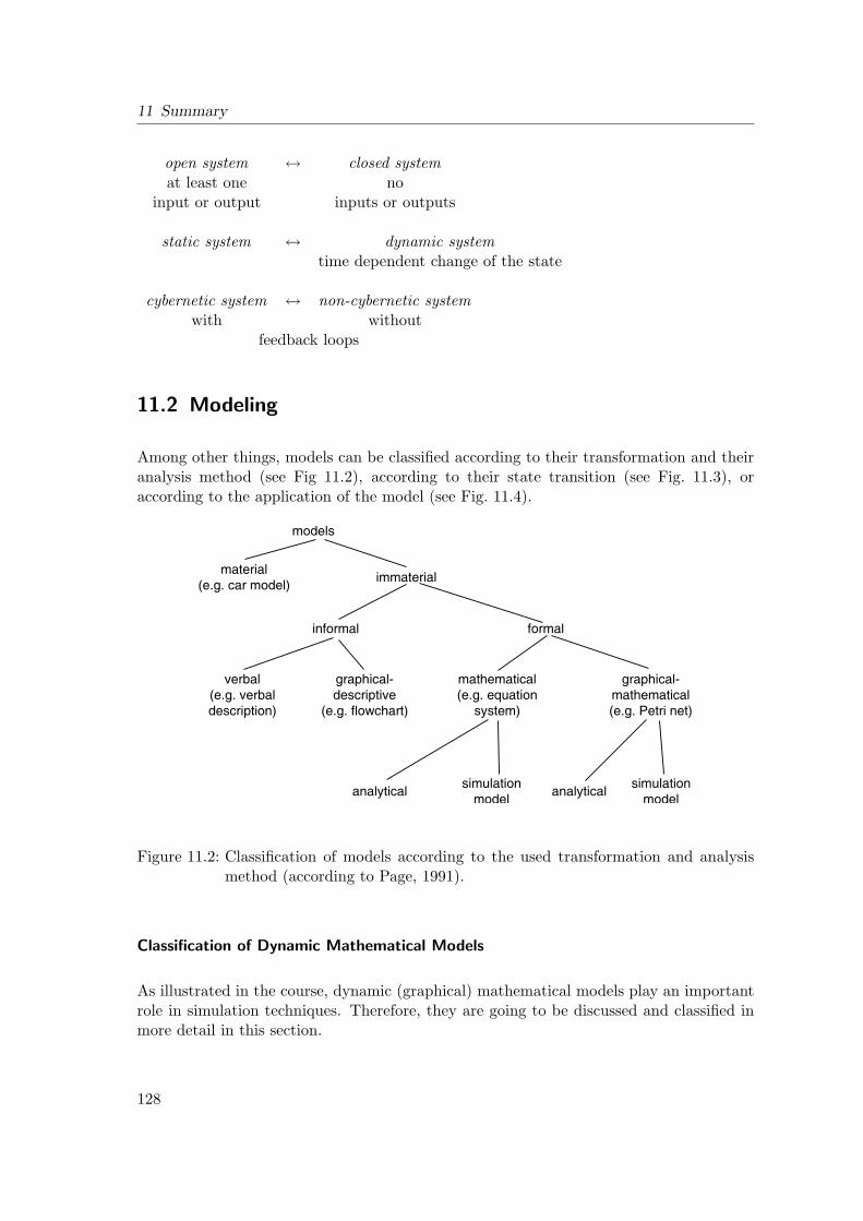
11 Summary
open system ↔ closed systemat least one no
input or output inputs or outputs
static system ↔ dynamic systemtime dependent change of the state
cybernetic system ↔ non-cybernetic systemwith without
feedback loops
11.2 Modeling
Among other things, models can be classified according to their transformation and theiranalysis method (see Fig 11.2), according to their state transition (see Fig. 11.3), oraccording to the application of the model (see Fig. 11.4).
Figure 11.2: Classification of models according to the used transformation and analysismethod (according to Page, 1991).
Classification of Dynamic Mathematical Models
As illustrated in the course, dynamic (graphical) mathematical models play an importantrole in simulation techniques. Therefore, they are going to be discussed and classified inmore detail in this section.
128
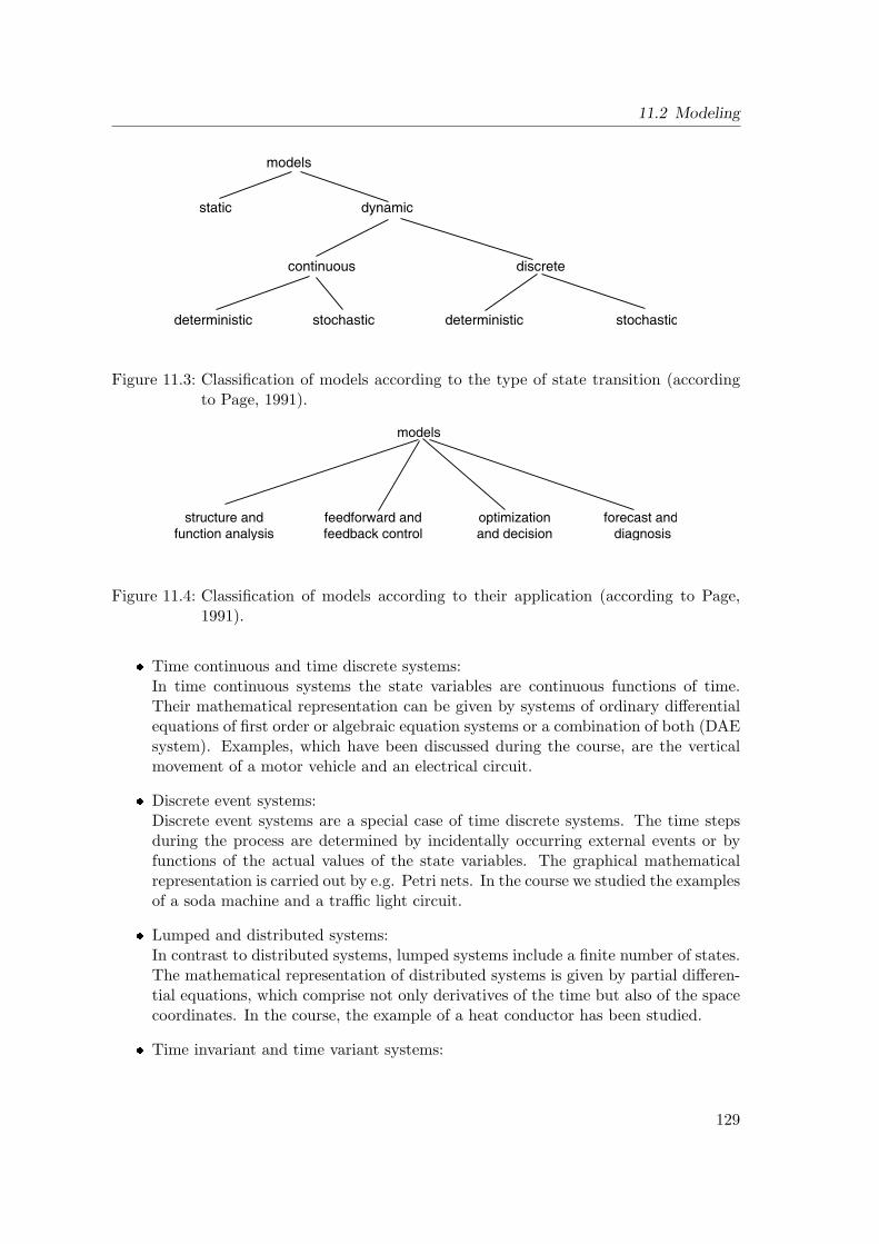
11.2 Modeling
Figure 11.3: Classification of models according to the type of state transition (accordingto Page, 1991).
Figure 11.4: Classification of models according to their application (according to Page,1991).
Time continuous and time discrete systems:In time continuous systems the state variables are continuous functions of time.Their mathematical representation can be given by systems of ordinary differentialequations of first order or algebraic equation systems or a combination of both (DAEsystem). Examples, which have been discussed during the course, are the verticalmovement of a motor vehicle and an electrical circuit.
Discrete event systems:Discrete event systems are a special case of time discrete systems. The time stepsduring the process are determined by incidentally occurring external events or byfunctions of the actual values of the state variables. The graphical mathematicalrepresentation is carried out by e.g. Petri nets. In the course we studied the examplesof a soda machine and a traffic light circuit.
Lumped and distributed systems:In contrast to distributed systems, lumped systems include a finite number of states.The mathematical representation of distributed systems is given by partial differen-tial equations, which comprise not only derivatives of the time but also of the spacecoordinates. In the course, the example of a heat conductor has been studied.
Time invariant and time variant systems:
129
11 Summary
In time invariant systems the systems function is independent of time (autonomoussystem). Therefore, the model parameters are time independent as well.
Linear and nonlinear systems:In linear systems the superposition principle holds true:
f(u1 + u2) = f(u1) + f(u2) (11.1)
The predator-prey model has been introduced as an example for a nonlinear model.
Steady-state and dynamic models:In contrast to dynamic models, the behavior of steady-state models is time indepen-dent. An example is a chemical reaction system.
11.3 Numerics
The numerical methods treated in the course shall be listed in note form in this section:
equation systems
– linear: Gauß elimination
– nonlinear: Newton-Raphson method
ordinary differential equation systems
– one-step method/multi-step method
– implicit/explicit method
differential-algebraic systems: solvability
partial differential equations
– method of lines, method of differences
– method of weighted residuals
discrete event systems
– graphical representation
– mathematical representation
11.4 Simulators
Simulation software can be distinguished according to different criteria:
130
11.4 Simulators
11.4.1 Application Level
Software on the level of programming languages:compilers or interpreters of a programming language, which is suitable for the im-plementation of simulation models (e.g. Matlab)
Software on the level of models:completely implemented models, only the input parameters are freely selectable (e.g.flight simulator)
Software on the level of support systems:integrated, interactive working environment (e.g. Simulink)
11.4.2 Level of Problem Orientation
universally usable software:e.g. compiler for general high-level programming languages
simulation specific software:software especially developed for the purpose of simulation (e.g. Simulink)
software oriented along specific classes of problems and specific model types
software oriented along the problem definition of one application domain
11.4.3 Language Level
general programming languagese.g. FORTRAN, C(++), PASCAL
Simulation packagescollection (library) of procedures and functions
Simulation languages
– low-level simulation languages
– high-level simulation languages: implementation of models is eased
– systems-oriented simulation language: direct modeling of specific system classes
11.4.4 Structure of a Simulation System
Fig. 11.5 shows the general structure of a simulation system. Thereby, the modules mod-eling component, graphical user interface, results analysis, model and method data base,experiment control, and simulation data base can be distinguished. Not all of these mod-ules have to be present in a simulation system. Furthermore, the complexity of thesemodules in different simulation systems varies significantly.
131
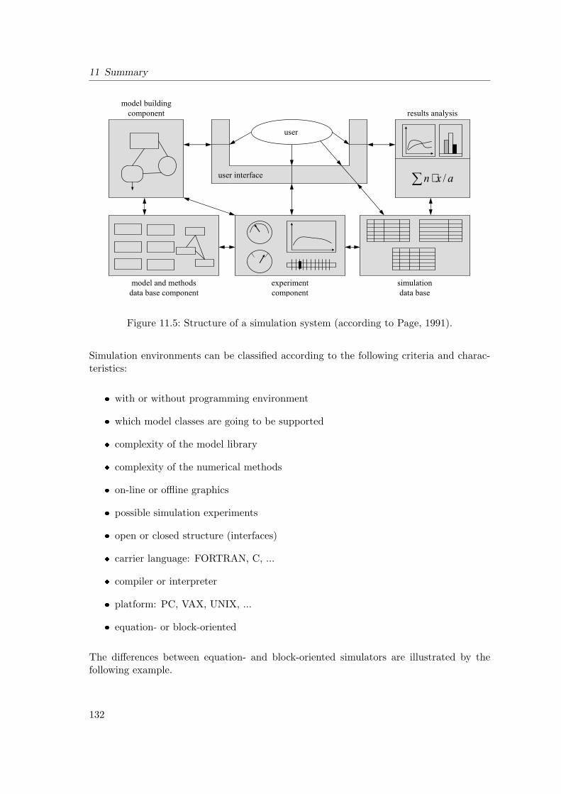
11 Summary
⋅
Figure 11.5: Structure of a simulation system (according to Page, 1991).
Simulation environments can be classified according to the following criteria and charac-teristics:
with or without programming environment
which model classes are going to be supported
complexity of the model library
complexity of the numerical methods
on-line or offline graphics
possible simulation experiments
open or closed structure (interfaces)
carrier language: FORTRAN, C, ...
compiler or interpreter
platform: PC, VAX, UNIX, ...
equation- or block-oriented
The differences between equation- and block-oriented simulators are illustrated by thefollowing example.
132
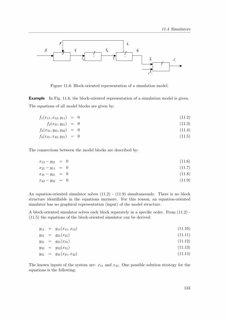
11.4 Simulators
!"
#$%
&'(
Figure 11.6: Block-oriented representation of a simulation model.
Example In Fig. 11.6, the block-oriented representation of a simulation model is given.
The equations of all model blocks are given by:
f1(x11, x12, y11) = 0 (11.2)f2(x21, y21) = 0 (11.3)
f3(x31, y31, y32) = 0 (11.4)f4(x41, x42, y41) = 0 (11.5)
The connections between the model blocks are described by:
x12 − y31 = 0 (11.6)x21 − y11 = 0 (11.7)x31 − y21 = 0 (11.8)x42 − y32 = 0 (11.9)
An equation-oriented simulator solves (11.2) - (11.9) simultaneously. There is no blockstructure identifiable in the equations anymore. For this reason, an equation-orientedsimulator has no graphical representation (input) of the model structure.
A block-oriented simulator solves each block separately in a specific order. From (11.2) -(11.5) the equations of the block-oriented simulator can be derived:
y11 = g11(x11, x12) (11.10)y21 = g21(x21) (11.11)y31 = g31(x31) (11.12)y32 = g32(x31) (11.13)y41 = g41(x41, x42) (11.14)
The known inputs of the system are: x11 and x41. One possible solution strategy for theequations is the following:
133
11 Summary
1. Estimate x12
2. Calculate y11, then y21, . . . , y31, y32
3. x12 − y31 =?
a) = 0: calculate y41
b) 6= 0: set x12 = y31 and repeat step 2
11.5 Parameter Identification
In parameter identification the parameters of a model are calculated in such a way, that thedifferences between simulated and measured values are going to be minimized. Therefore,these differences have to be squared and summarized in an objective function. With theuse of some calculation algorithm one tries to minimize this objective function. Thereby,two cases can be distinguished:
direct solution: (weighted) least squares method
indirect solution using optimization methods
11.6 Use of Simulators
The major reasons for the use of simulators are:
The system is not available.
Experiments within the system are too dangerous.
The experiment costs are too high.
The time constants of the system are too large.
The variables of interest are difficult to measure or not measurable at all.
There are disturbances within the real system.
134
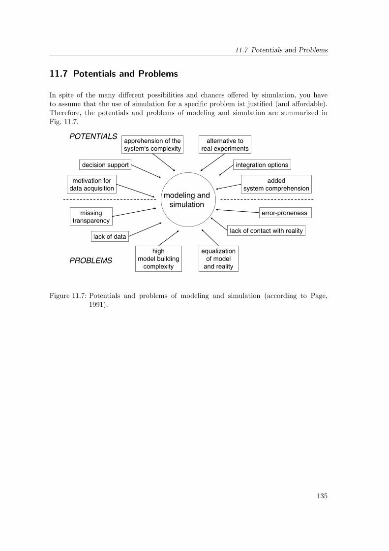
11.7 Potentials and Problems
11.7 Potentials and Problems
In spite of the many different possibilities and chances offered by simulation, you haveto assume that the use of simulation for a specific problem ist justified (and affordable).Therefore, the potentials and problems of modeling and simulation are summarized inFig. 11.7.
Figure 11.7: Potentials and problems of modeling and simulation (according to Page,1991).
135

11 Summary
136
Bibliography
Astrom, K., Elmqvist, H. and Mattsson, S. (1998). Evolution of continuous-time modelingand simulation, 12th European Simulation Multiconference, ESM’ 98, Manchester,pp. 1–10.
Bachmann, B. and Wiesmann, H. (2000). Objektorientierte Modellierung PhysikalischerSysteme, Teil 15, at - Automatisierungstechnik 48: A57–A60.
Bauknecht, K., Kohlas, J. and Zehnder, C. (1976). Simulationstechnik, Springer, Berlin.
Beater, P. (2000). Objektorientierte Modellierung Physikalischer Systeme, Teil 10, at -Automatisierungstechnik 48: A37–A40.
Bennett, B. (1995). Simulation Fundamentals, Prentice Hall. bestellt, 10.7.00.
Bischoff, K. and Himmelblau, D. (1967). Fundamentals of Process Analysis and Sim-ulation, number 1 in AIChE Continuing Education Series, American Institute ofChemical Engineers, New York.
Bossel, H. (1992). Modellbildung und Simulation, Vieweg & Sohn Verlagsgesellschaft mbH,Braunschweig.
Bratley, P., Fox, B. and Schrage, L. (1987). A Guide to Simulation, Springer, New York.
Breitenecker, F., Troch, I. and Kopacek, P. (eds) (1990). Simulationstechnik, Vieweg,Braunschweig.
Cellier, F. (1992). Simulation modelling formalism: Ordinary differential equations, inD. Atherton and P. Borne (eds), Concise Encyclopedia of Modelling & Simulation,Pergamon Press, Oxford, pp. 420–423.
Clauß, C., Schneider, A. and Schwarz, P. (2000a). Objektorientierte ModellierungPhysikalischer Systeme, Teil 13, at - Automatisierungstechnik 48: A49–A52.
Clauß, C., Schneider, A. and Schwarz, P. (2000b). Objektorientierte ModellierungPhysikalischer Systeme, Teil 14, at - Automatisierungstechnik 48: A53–A56.
Dahmen, W. (1994). Einfuhrung in die numerische Mathematik (fur Maschinenbauer),Institut fur Geometrie und Praktische Mathematik, RWTH Aachen.
Engeln-Muller, G. and Reutter, F. (1993). Numerik-Algorithmen mit Fortran 77-Programmen, BI Wissenschaftsverlag, Mannheim.
137
Bibliography
Fishman, G. (1978). Principles of Discrete Event Simulation, John Wiley, New York.
Follinger, O. and Franke, D. (1982). Einfuhrung in die Zustandsbeschreibung dynamischerSysteme, Oldenbourg, Munchen.
Fritzson, P. (1998). Modelica - a language for equation-based physical modeling andhigh performance simulation, APPLIED PARALLED COMPUTING 1541: 149–160.bestellt, 10.7.00.
Fritzson, P. and Engelson, V. (1998). Modelica - a unified object-oriented language for sys-tem modeling and simulation, ECOOP’98 (the 12th European Conference on Object-Oriented Programming).
Gipser, M. (1999). Systemdynamik und Simulation, B.G: Teubner, Stuttgart.
Gordon, G. (1969). System Simulation, Prentice-Hall, Englewood Cliffs.
Hanisch, H.-M. (1992). Petri-Netze in der Verfahrenstechnik, Oldenbourg, Munchen.
Hoffmann, U. and Hofmann, H. (1971). Einfuhrung in die Optimierung, Verlag Chemie,Weinheim.
Hohmann, R. (1999). Methoden und Modelle der Kontinuierlichen Simulation, Shaker,Aachen.
Holzinger, M. (1996). Modellorientierte Parallelisierung von Modellen mit verteilten Pa-rametern, Master’s thesis, Technische Universitat Wien.
Jain, R. (1991). The Art of Computer Systems Performance Analysis: Techniques forExperimental Design, Measurement, Simulation, and Modeling, John Wiley & Sons,New York.
Kiencke, U. (1997). Ereignisdiskrete Systeme, Oldenbourg, Munchen.
Kocher, D., Matt, G., Oertel, C. and Schneeweiß, H. (1972). Einfuhrung in die Simula-tionstechnik, Deutsche Gesellschaft fur Operations Research.
Korn, G. and Wailt, J. (1983). Digitale Simulation kontinuierlicher Systeme, Oldenbourg,Munchen.
Kramer, U. and Neculau, M. (1998). Simulationstechnik, Carl Hanser, Munchen.
Lapidus, L. and Pinder, G. (1982). Numerical Solution of Partial Differential Equationsin Science and Engineering, John Wiley & Sons, New York.
Law, A. and Kelton, W. (1991). Simulation Modeling and Analysis, McGraw Hill, NewYork.
Lehman, R. (1977). Computer Simulation and Modeling: An Introduction, LawrenceErlbaum, Hillsdale.
138
Bibliography
Liebl, F. (1992). Simulation - Problemorientierte Einfuhrung, Oldenbourg, Munchen.
Lotka, A. J. (1925). Elements of Physical Biology, Williams and Wilkins, Baltimore.
Margolis, D. (1992). Simulation modelling formalism: Bond graphs, in D. Atherton andP. Borne (eds), Concise Encyclopedia of Modelling & Simulation, Pergamon Press,Oxford, pp. 415–420.
Marquardt, W. (1991). Dynamic process simulation - recent progress and future challenges,in W. Ray and Y. Arkun (eds), Chemical Process Control - CPC IV.
MathWorks (2000). Using MATLAB, Version 6, The MathWorks, Inc., Natick, USA.
MathWorks (2002). Simulink for model-based and system-level design. Product informa-tionen online available at http://www.mathworks.com/ (viewed 25 March 2002).
Meadows, D. L., Meadows, D. H. and Zahn, E. (2000). Die Grenzen des Wachstums.Club of Rome. Bericht des Club of Rome zur Lage der Menschheit, Deutsche Verlags-Anstalt.
Mezencev, R. (1992). Simulation languages, in D. Atherton and P. Borne (eds), ConciseEncyclopedia of Modelling & Simulation, Pergamon Press, Oxford, pp. 409–415.
Minsky, M. (1965). Matter, mind and models, in A. Kalenich (ed.), Proceedings Interna-tional Federation of Information Processing Congress, Spartan Books, Washington,pp. 45–49.
Moller, D. (1992). Modellbildung, Simulation und Identifikation dynamischer Systeme,Springer, Berlin. bestellt, 22.9.00, nicht nachweisbar.
Nidumolu, S., Menon, N. and Zeigler, B. (1998). Object-oriented business process modelingand siumlation: A discrete event system specification framework, Simulation Practiceand Theory 6: 533–571.
Norton, J. (1997). An Introduction to Identification, Academic Press.
Odum, H. and Odum, E. (2000). Modeling for All Scales: An Introduction to SystemSimulation, Academic Press, San Diego.
Otter, M. (1999a). Objektorientierte Modellierung Physikalischer Systeme, Teil 1, at -Automatisierungstechnik 47: A1–A4.
Otter, M. (1999b). Objektorientierte Modellierung Physikalischer Systeme, Teil 2, at -Automatisierungstechnik 47: A5–A8.
Otter, M. (1999c). Objektorientierte Modellierung Physikalischer Systeme, Teil 3, at -Automatisierungstechnik 47: A9–A12.
Otter, M. (1999d). Objektorientierte Modellierung Physikalischer Systeme, Teil 4, at -Automatisierungstechnik 47: A13–A16.
139
Bibliography
Otter, M. (2000). Objektorientierte Modellierung Physikalischer Systeme, Teil 17, at -Automatisierungstechnik 48: A65–A68.
Otter, M. and Bachmann, B. (1999a). Objektorientierte Modellierung Physikalischer Sys-teme, Teil 5, at - Automatisierungstechnik 47: A17–A20.
Otter, M. and Bachmann, B. (1999b). Objektorientierte Modellierung Physikalischer Sys-teme, Teil 6, at - Automatisierungstechnik 47: A21–A24.
Otter, M., Elmqvist, H. and Mattson, S. (1999). Objektorientierte ModellierungPhysikalischer Systeme, Teil 8, at - Automatisierungstechnik 47: A29–A32.
Otter, M., Elmqvist, H. and Mattsson, S. (1999). Objektorientierte ModellierungPhysikalischer Systeme, Teil 7, at - Automatisierungstechnik 47: A25–A28.
Otter, M. and Schlegel, M. (1999). Objektorientierte Modellierung Physikalischer Systeme,Teil 9, at - Automatisierungstechnik 47: A33–A36.
Page, B. (1991). Diskrete Simulation. Eine Einfuhrung mit Modula-2, Springer, Berlin.
Piehler, J. and Zschiesche, H.-U. (1976). Simulationsmethoden, BSB B.G. Teubner,Leipzig.
Press, W. H., Flannery, B. P., Teukolsky, S. A. and Vetterling, W. T. (1990). NumericalRecipes - The Art of Scientific Computing, Cambridge University Press, Cambridge.
Roberts, N. e. A. (1994). Introduction to Computer Simulation: A System DynamicsModeling Approach, Productivity Press. bestellt, 10.7.00.
Sadoun, B. (2000). Applied system simulation: A review study, Information Sciences124: 173–192.
Savic, D. and Savic, D. (1989). BASIC Technical Systems Simulation, Butterworth & Co,London.
Schiesser, W. (1991). The Numerical Method of Lines, Academic Press, San Diego.
Schneider, R. (1999). Untersuchung eines adaptiven pradiktiven Regelungsverfahrenszur Optimierung von bioverfahrenstechnsichen Prozessen, Fortschritt-Berichte VDI,Reihe 8, Nr. 855, VDI Verlag, Dusseldorf.
Schone, A. (1973). Simulation Technischer Systeme, Carl Hanser. bestellt, 7.7.00.
Schumann, R. (1998). CAE von Regelsystemen, atp - Automatisierungstechnische Praxis40: 48–63.
Schwarze, G. (1990). Digitale Simulation, Akademie-Verlag, Berlin.
Shannon, R. (1975). Systems Simulation: The Art and Science., Prentice Hall, EnglewoodCliffs.
140
Bibliography
Tummescheit, H. (2000a). Objektorientierte Modellierung Physikalischer Systeme, Teil11, at - Automatisierungstechnik 48: A41–A44.
Tummescheit, H. (2000b). Objektorientierte Modellierung Physikalischer Systeme, Teil12, at - Automatisierungstechnik 48: A45–A48.
Tummescheit, H. and Tiller, M. (2000). Objektorientierte Modellierung PhysikalischerSysteme, Teil 16, at - Automatisierungstechnik 48: A61–A64.
Tzafestas, S. (1992). Simulation modelling formalism: Partial differential equations, inD. Atherton and P. Borne (eds), Concise Encyclopedia of Modelling & Simulation,Pergamon Press, Oxford, pp. 423–428.
Verein Deutscher Ingenieure (1996). VDI-Richtlinie 3633: Simulation von Logistik-,Materialfluß- und Produktionssystemen - Begriffsdefinitionen.
Volterra, V. (1926). Variations and fluctuations of the number of individuals in animalspecies living together, in C. R. N. (ed.), Animal Ecology, McGraw-Hill, New York,pp. 409–448.
Watzdorf, R., Allgower, F., Helget, A., Marquardt, W. and Gilles, E. (1994). DynamischeSimulation verfahrenstechnischer Prozesse und Anlagen -Ein Vergleich von Werkzeu-gen, in G. Kampe and M. Zeik (eds), Simulationstechnik, 9.ASIM-Symposium inStuttgart, pp. 83–88.
Wollhaf, K. (1995). Objektorientierte Modellierung und Simulation verfahrenstechnischerMehrproduktanlagen, Shaker, Aachen.
Woolfson, M. and Pert, G. (1999). An Introduction to Computer Simulation, OxfordUniversity Press, New York.
Zeigler, B. (1984a). Multifacetted Modelling and Discrete Event Simulation, AcademicPress, chapter Multifacetted Modelling: Motivation and Perspective, pp. 3–19.
Zeigler, B. (1984b). Multifacetted Modelling and Discrete Event Simulation, AcademicPress, chapter System Architectures for Multifacetted Modelling, pp. 335–371.
Zeitz, M. (1999). Simulationstechnik. Lecture notes, Institut fur Systemdynamik undRegelungstechnik, Universitat Stuttgart.
141