introduction - s u · web viewrt,t+m denotes the time t forecast of a return for period t+m. ft,t+m...

1. INTRODUCTION

1.1 PURPOSE1.1.1 METHOD

2. VALUE AT RISK

2.1 INTRODUCTION TO THE VALUE AT RISK CONCEPTION2.2 VALUE AT RISK MODELS

3. HISTORIC SIMULATION

4. RISK METRICS

4.1 RISK METRICS OVERVIEW4.2 RISK ASSOCIATED WITH A PORTFOLIO OF ASSETS4.3 DAILY EARNINGS AT RISK (DEAR)4.4 VAR IN RESPECT TO DEAR4.5 METHOD FOR VOLATILITY ESTIMATION4.6 RISK METRICS - APPLIED ON EQUITY

4.6.1 THE THEORY4.7 THE RISK METRICS METHODOLOGY FOR OPTIONS

4.7.1 OPTIONS’ VAR USING DELTA/GAMMA APPROXIMATION.

5. MONTE CARLO SIMULATION

5.1 GENERATING SCENARIOS FROM STATISTICS5.1.1 THE THEORY5.1.2 APPLIED MONTE CARLO

6. THE BASLE PROPOSAL

7. THE SIMULATIONS

7.1 THE 'ACTUAL VAR LEVEL'7.2 BASIC ASSUMPTIONS FOR THE SIMULATIONS7.3 INTRODUCING THE SIMULATIONS7.4 PORTFOLIO 1 - FOREIGN EXCHANGE7.5 PORTFOLIO 2 - TREASURY BILLS7.6 PORTFOLIO 3 - STOCK INDICES7.7 PORTFOLIO 4 - EQUITY7.8 PORTFOLIO 5 - CURRENCY OPTIONS7.9 PORTFOLIO 6 - EQUITY OPTIONS

8. SUMMARY AND CONCLUSION

9. APPENDIX

9.1 OUR OWN SOLUTION TO RISK METRICS’ OPTION PROBLEM - THE RM9.1.1 THE THEORY BEHIND RM9.1.2 THE RMIN PRACTICE

10. SOURCES

2

A Quantitative Analysis of Value at Risk Models

1Introduction

Value at Risk (VaR) has become a widely adapted risk management tool the last years. VaR is a measure that can be adopted on different instruments and can be related to by anyone within the organization, both at the trading desk as by the management. This can be accomplished by expressing portfolio risk as a statistical estimate on how much a given portfolio can decline in value at a given time horizon and confidence interval. For instance, a portfolio of positions could with 95% probability lose less than X amount of USD in one week. All large banks in Sweden that the authors of this paper have been in contact with, have projects or even business departments that addresses this issue.

In “Risk Metrics - Will it Do as a Global Benchmark?”, we evaluated the JP Morgan version of VaR, Risk Metrics, and commented on the criticism that have been raised from both the academic society as well as competitors to JP Morgan. We also gave a rather comprehensive description of the statistical assumptions and quantitative analysis behind Risk Metrics and alternative models. Two main questions were raised while writing that paper. The first is the ability to apply VaR on different instruments. There is no doubt that VaR is a smooth tool for all instruments, but does it really give sufficient precision? A large Swedish bank uses VaR on their derivatives portfolios, but is VaR really the answer to the control of derivatives market risk? The other question were the effect of different length of the risk horizon. A lot of the research in this area have been done by the financial institutions themselves on their own existing portfolios. Of natural reasons, they are not always that enthusiastic to share their results, due to the competition in this area and secretes of their portfolios.

During the work with our first thesis we found that there were a lot of analysis’s published but they all focused on comparing different VaR methodologies at one specific date1. Hence, the only thing that could be analyzed was their relative order of magnitude, not the concept itself. Instead, since VaR is a statistical estimate, we decided to examine different models’ ability to predict future market risk over a long period of time. We mean, that VaR has to be evaluated under a period of time to really se how it works. Dynamic tools should be evaluated under dynamic conditions. Otherwise you risk to be trapped in the same static thinking that VaR is meant to avoid.

In this paper we will give answers to these questions by doing a quantitative analysis on different portfolios containing a vary of instruments. We will also use four different models to calculate VaR on each of the portfolios to see what conclusions can be drawn.

We will assume that the reader has knowledge of established statistical theory like Gaussian distributions, leptokurtosis etc. It will also be an advantage to have a basic understanding of the concept of Value at Risk. We recommend to have read our earlier work in advance, where a lot have been explained in greater detail than it will be here.

1.1Purpose

The main purpose with this paper is to find out if the concept of VaR is valid for four different risk models, Historic simulation, Monte Carlo simulation, Risk Metrics and the Basle method. To what extent can you trust the given confidence interval, and how consistent are the estimations?

1 Styblo Beder (1995), “VaR: Seductive but dangerous”, Financial Analyst Journal Sep-Oct p.12-24

3

Also, we have reason to verify the differences between linear and derivative instruments that we saw in our work, as well as the problems connected to varying correlations and time horizons. We will also identify if some method is superior on one instrument/ timehorizon but questionable on one other. We have reasons to suspect that a portfolio manager have different investment horizons than a regular trader. Hence, it is interesting to know how the time horizon affects the efficiency. These are essential questions for the whole concept of Value at Risk.

1.1.1Method

The VaR concept can be implemented on a number of instruments where market risk has to be controlled. We have selected some of the most usual financial instruments on the market and from these, more complex positions can be derived. These instruments are: FX-spot, stocks (single as well as indices), Treasury bills, and options on stocks and currencies.

To capture the effects of diversification, all portfolios consists of instruments from four different markets: Germany, Japan, Sweden and the United States. These countries show good liquidity and they are often included in a Swedish investment portfolio. Hence, we use DEM, JPY, SEK and USD in the currency and bond portfolios.

In our quantitative analysis we compare the estimated VaR for each method to the actual market risk that appear at the end of the risk horizon. We will refer to these expressions as ex-ante market risk and the latter to ex-post market risk. To see how well the ex-ante market risk responds to the ex-post, we compute the number of days where the ex-post market risk exceeds the ex-ante. The result is expressed as a ratio, the computed number of days divided by the total number of days. With a 95 percent confidence level the ex-post Value at Risk should equal five percent to be a perfect match.

We have used Matlab 4.2c software for our calculations. There are two reasons for this decision: First we didn’t want any computer programming problems. Matlab is a so called highlevel language and it is very easy to use. Second, Matlab has a lot of prespecified functions that we were interested in, for example sorting functions and a random generator. The disadvantage of Matlab is that it’s not a fast language. For some of our calculations it would probably be more appropriate using Fortran or C if the processor resources are limited.

All our calculations are made at the Royal Institute of Technology in Stockholm at SPARC station 5 computers from SUN. Some of the methods are quite computer intensive and this should be a factor to take under consideration.

4


2Value at Risk

Financial markets of today are nothing like they used to be. Faster trades, instant and equal information all around the world and an exceptional increase in volume, has totally changed the conditions for all counterparts. The danger with such a fast development is that some areas that is not driven by market force, may be neglected and obsolete. Risk management could be such an area. It is easy to forget if you haven’t suffered any losses. Lately we have seen examples of that it can come as a surprise and cause substantial financial difficulties. Under these new market conditions, we need a tool that captures the dynamics in today’s financial markets. VaR could be such a tool.

2.1Introduction to the Value at Risk Conception

VaR is easy to relate to for anyone within the organization. Basically it describes in one figure how much, expressed as USD or any currency, you risk to loose, which means that it is usable as a benchmark. Benchmarks is a useful tool in a number of situations, also in the world of risk management. This could lead to that instead of referring to complex formulas, shareholder and management among others would speak the same language. The rest of this chapter will explain the theories behind this tool.

VaR is a statistical estimate, for a given level of probability, of how much a firm risks losing over a specified period of time due to changes in market price.

One of the key advantages of VaR is that it looks at risk over time, based on historical data, rather than simply providing a static snapshot of a portfolio or a balance sheet. Most VaR models assume that the value of a portfolio, on average, is random and its frequency distribution can be estimated using a normal, or Gaussian, statistical curve.

Given the volatility of the financial instruments and the correlation between them a time and a confidence interval, the market risk can be calculated. The confidence interval is the probability of avoiding a loss equal to or greater than the VaR over the time horizon. ItÕs important to emphasize that all calculations are based on historical data, and there are a number of ways to predict and evaluate volatility. In our first study, we gave a detailed description of different volatility estimation methods and empirical research in the matter. From this research, we found that the exponential smoothing approach gives sufficient prediction ability and for all VaR models, except for the Basle, we use it with a decay factor of 0.94.

2.2Value at Risk Models

The VaR is a statistical estimate and is based on historical data, it is not precisely known, hence different models can be used for the estimation. In this section, we briefly present the four methods that weÕre using in our analysis, their theories in detail are introduced in the forthcoming chapters.

Historic Simulation - Given a series of historical market data prices, the Historic Simulation VaR is derived from the distribution of portfolio values over a specified time horizon. First, compute the portfolioÕs total return, which is the change in Net Present Value (NPV) between the date and the next, depending on the risk horizon. There are two main alternatives to obtain the estimated risk. Either assume normality and calculate the standard deviation to receive a confidence interval, or we just identify the fifth or first percentile of the portfolio value distribution. In our analysis we use both methods, which differ significantly in some important situations.

5

The Correlation Method (Variance / Covariance method - Risk Metrics) - All financial instruments can be split up in cash flows occurring at a specific times. By calculating volatilities and correlations for every single cash flow, you retrieve enough information to by simple matrix algebra, calculate a zero coupon equivalent which represents the diversified VaR.

Monte Carlo simulation - By creating lognormal changes in specified risk factors, a large number of scenarios are generated, which are applied on the portfolio. Then, if we are interested in a confidence interval of 95%, the fifth percentile of the distribution represents the VaR.

The Basle Method - The Bank of International Settlements (BIS)2 has made a proposal that says that VaR methods with some modifications can be used instead of capital adequacy requirements. The basics are: one year equally weighted observations used for volatility, correlations between asset classes are set to 1 or -1, a 1% confidence interval is used, and at last, the diversified VaR should be multiplied by three.

2 BIS works as a co-operation between the central banks of Europe.

6


3Historic Simulation

Historic Simulation is the most direct technique for computing VaR. The advantage of the approach is that it is universal - it is applicable to all instruments and all market price risk types. Statistically, Historic Simulation VaR is derived from the distribution of portfolio values over a specified time horizon, given a series of historical market data prices. The choice of a time period is a balancing act between increasing the sample size to capture a full variety of events and relationships between factors, and using a period that is too long so that the events and relationships observed are not representative of what can be expected in the future. In our VaR analysis weÕre using a period of 100 days. There are two reasons for this: First, it is a rather natural assumption because it creates the fifth and first percentile to be the fifth and first worst case respectively, and it will capture the changes over a five month window. Second, the Chase Manhattan Bank uses a type of Historic Simulation based on a 100 day window.

The distribution of portfolio values is calculated by revaluing the portfolio many times using time series of market prices. Portfolio total return is measured as the change in market value between one date and the next, as determined by the length of time horizon.

(3.1) NPVi=(1...n) = NPVi+t-NPVi

where

i = begin date in time series n = total number of days in time series t = time horizon in days

Once the time series of NPV (Net Present Value) changes is computed, several possible techniques can be used to determine the probability of loss. In our VaR analysis we examine two different methods, the standard deviation and the worst case approach. If normality is assumed (the most common approach), we compute the standard deviation of NPV changes, and from this, the estimated VaR for any confidence interval can be calculated using the cumulative normal distribution.

Table 3.1.aCalculating VaR from Historic Simulation with Standard Deviation

1. Generate the NPV changes for your portfolio from equation 3.1.2. Assume normality and calculate the standard deviation. We use both the exponential smoothing

method and a standard deviation based on equal weights.3. Compute the confidence interval which is -1.65 standard deviations on the 95% level and -2.33

standard deviations on the 99% level.

7

Instead of utilize the normal curve as a result the probable loss can also be computed from the histogram of actual daily NPV changes. This is the only method that uses past data without first converting them into statistical equivalents for the purpose of estimation. The 5 percent worst case scenarios, for instance, can be calculated directly from the data series - just identify the fifth percentile point in the histogram.

Table 3.1.bCalculation scheme for Historic Simulation with Worst Case

1. Generate the NPV changes for your portfolio from equation 3.1.2. Sort the distribution in order of magnitude.3. Take the fifth and first percentile from the histogram.

In our simulations, we compute three different VaR for Historic Simulation at each confidence level: one based on the worst case approach and two derived from standard deviations with equal weights and exponential smoothing respectively.

The Historic Simulation approach is attractive because it is not sensitive to the three assumptions on which the correlation / Risk Metrics method is based.

· As actual changes in underlying prices are used, we can capture all outlier events that occurred over the historical period, rather relying on a standard deviation that could potentially understate risk by not properly capturing the tail events.

· We also capture the actual covariation between risk factors, both typical correlation relationships and the times when those break down.

· The use of a multi-point price sensitivity captures the dynamic delta effects and gives a true picture of the price risk profile of the portfolio.

8


4Risk Metrics

Risk Metrics was introduced by JP Morgan in October 1994 and is based on correlation/covariance method. Daily updated datasets with correlations and volatilities on a large number of assets are distributed free on the Internet3 to anyone that is interested. The purpose with this initiative is to create a global benchmark for market risk, which of course if they manage will have a positive effect on their main business. Below, we explain the fundamentals of Risk Metrics.

4.1Risk Metrics Overview

Risk Metrics is a tool to map financial positions and estimate their market risk, that is the uncertainty of earnings resulting from changes in market conditions (interest rates, price of the asset, volatility). The market risk can be expressed as a potential loss in a currency (absolute market risk) over a certain time horizon. The time horizon can be as short as one day for trade managers, and months for longer investment or instruments that take longer time to unwind. We will analyze several alternative risk horizons later in chapter 7.

One major statistical assumption is that returns are jointly normally distributed. By making this statement probabilities can easily be calculated along with existing theories. Risk Metrics applies a 95 percent confidence interval which means that on the average 19 days of 20, the potential loss will be less than the calculated risk.

The basic idea is to break down every single position into cash flows to specific time horizons for every currency. There are fifteen different horizons, from one day until 16 years. Risk Metrics publishes data on volatility and yield for each date. Each currency and time horizon interacts and creates a correlation matrix which is important to consider while calculating the diversified risk. The thought is to predict how all currencies and yields will interact at different occasions in the future. This interaction requires calculated correlations between every possible combination of currency, yield, date and instrument.

Using all the data corresponding to the instruments involved, the cash flows are summarized in one DEaR4 vector of individual positions and one corresponding correlation matrix for this vector. Using standard matrix algebra, we can calculate a diversified Daily Earnings at Risk that is lower than the undiversified. Hence the result will show how much you can loose in one single currency with a probability of 95 percent. The formula used for the diversified DEaR is showed in equation 4.5.

3 The address to JP Morgan’s homepage is: www.jpmorgan.com4 DEaR is simply the VaR for a one day risk horizon.

9

4.2Risk Associated with a Portfolio of Assets

One way to think about VaR and the Correlation Method is to imagine a given portfolio, pushing historical prices through it and reevaluating it each day. The portfolio may not change, but its implied market value does, based on the different prices each day. The daily change in value, or net present value (NPV) walking through time is then computed and stored in a time series. The standard deviation is then calculated. Once this is known, itÕs easy to estimate the probability of a given loss over the next day for a given confidence interval. By covariance/correlation analysis itÕs possible to compress all bonds, swaps, derivatives and foreign exchange into one master transaction per currency, with a cash flow at desired date. This can reduce the number of necessary reevaluations by orders of magnitude.

To calculate the risk of a portfolio of assets we obviously need to have some understanding of how returns move in relation to each other. In general, the risk of a portfolio consisting of N assets depends on the correlation between the assetsÕ returns. The value of this portfolio can be written as the summation of N correlated random returns (variables). Moreover, we weight each return according to the amount invested in its underlying asset.

For example, the value of portfolio P is expressed as:

(4.1) P Xii

N

i

1

where

Xi = return on asset ii = amount invested in asset i (position value)

The generalized portfolioÕs standard deviation is given by

(4.2) P i i i j ij i ji ji

N

2 2

12

i i i j iji ji

N

Cov2 2

12

where

i2 = variance of return i

ij = correlations between returns i and jCovij = covariance between returns i and j

Recall that the connection between the covariance and correlation follows:

(4.3) ij Cov ij

i j

Having obtained an expression for the diversified volatility of a portfolio, we can now treat the portfolio as if it were a single instrument. Therefore, the adverse rate move of the portfolio with 95% confidence would not be less than -1.65 standard deviations. For 99% confidence we have -2.33 standard deviations.

10


It is important to note that in our analysis, we are calculating with covariances instead of correlations. By this, we avoid an unnecessary computation path from by first get the covariance, then calculate the correlation and after that back again to the covariance. This problem is however not relevant if the datasets provided by JP Morgan are used.

4.3Daily Earnings at Risk (DEaR)

In most developed and liquid markets, positions can be unwound or neutralized within a day. Risks therefore are related to a 24-hour window. Risk Metrics define Daily Earnings at Risk (DEaR) as the estimated potential loss of a portfolioÕs value resulting from an adverse move in market factors over a one-day unwind period. After calculating DEaR, VaR can easily be derived for different time horizons as we will show in the next section.

In general, DEaR for a single position is calculated as follows:

(4.4) VaRx= Market value of position X (Mvx) * Sensitivity to price move per $ market value (d) * Adverse price move per day (Xa) = Mvx * d * Xa

Note that d measures the change in the market value of a position when the underlying price (or rate) changes. For cases where the value of the position is linearly related to the underlying price, d=1.

In general, the DEaR of a portfolio consisting of N assets, each asset having a DEaR i

(i=1,2,...,N) is calculated as follows.:

(4.5) DEaR V C VdiversifiedT

* *

where

V DEaR DEaRi N ...

CN

N

11

1

1

1

.... ..

..

VDEaR

DEaRN

1

..

This formula is basically the same as equation (4.2) with the inclusion of each variance now is multiplied by its currency cash flow expressed in dollars.

11

4.4VaR in Respect to DEaR

In many situations, positions cannot be unwound over 24 hours or the decision horizon (as in investment management) is longer than a day.

For trading purposes that cannot be neutralized or liquidated within a day, the most common practice is to multiply the daily risk estimate by the square root of the time required to unwind the position. We thus define Value at Risk (VaR) as the total risk over the unwind period if this is deemed to be more than one day.

(4.6) VaR = DEaR * (unwind period)1/2

where the unwind period is expressed in days.

This adoption should only be used for linear positions. If, as in options, a positionÕs value changes in a non-linear fashion relative to underlying prices, then this linear scaling of the daily risk may not be a good approximation for risks over longer periods.

4.5Method for Volatility Estimation

The simplest and most popular method for forecasting the volatility of a series is to take its historical volatility over a certain period with equal weights on past observations. JP Morgan uses an extended alternative which includes exponentially moving average.

Instead of applying the same weight to each data point as in simple moving average, the exponential moving average places relatively more weight on recent observations. The weight allocated to each data point depends on the value of the decay factor.

Consider a time series of observations {Xt} where the weights decline exponentially by the factor wj:

(4.7) X Xt j t jj

w0

where w jj 1 0<<1

where is a decay factor or discount coefficient and the wjÕs are a set of weights which sum to unity.

Risk Metrics publishes two optimized decay factors, one for daily volatilities and correlations and one for monthly. There are two reasons for this. First, JP Morgan wants to create a risk management tool which is fairly easy to understand. Second, if different decay factors are used for each time series then it is possible to get correlations which are greater than 1 in absolute value, i.e. the correlation matrix is not positive definite. With different decay factors the equation (4.5) for the diversified DEaR does not hold theoretically. All calculations must be based on the same benchmark, otherwise an error will be introduced in the VaR / DEaR calculations.

The method for estimation of volatility has been under heavy criticism from opponents who argue that more sophisticated approaches like GARCH would be superior to the exponentially smoothing. From the empirical research we have gone through however, we find that Risk Metrics estimated volatilities give sufficient prediction ability 5. Especially considering that the proposed alternatives are substantially more intensive, both in data inputs and calculation.

5 See the study by Boudoukh, Richardson and Whiteslaw (1995) which is included in our first thesis. Risk Metrics-Will It Do as a Global Benchmark?

12


For infinitely long windows, i.e. T approaching infinity the standard deviations derived from an exponential moving average have one additional advantage: they can be calculated recursively. That is, the standard deviation estimate at time t can be derived from the standard deviation estimate at time t-1, adjusted for the latest observation. Assuming a zero mean6:

(4.8) ~ wt ii

t iX2

0

2

1 21

2 X t t~

where

tt

t

PP

1001

ln

Computing the volatility requires an initial value 02. For this we use the simple equal

weighted variance according to:

(4.9) ~ 02

0

1 21

KX t i

i

K

Deriving the daily covariance forecasts proceed in a manner similar to the daily standard deviation estimates. As with the daily volatilities, an initial value of the covariances is needed. For our VaR analysis we use K=74 days to compute the initial variance, both for volatility and covariance estimates. JP Morgan has optimized the value of the decay factor to 0.94 for daily volatilities and we are using it in our calculation programs.

4.6Risk Metrics - Applied on Equity

The Risk Metrics concept includes all kind of instruments, even stocks and stock indices. Since there exists several thousands of stocks on different markets all over the world, Risk Metrics could not calculate correlation coefficients between all of them. Therefore, they have used the Capital Asset Pricing Model (CAPM) 7 to reduce the correlations necessary to include only the stock market indices as risk factors. In this chapter we will show how this works for stock indices as well as for specific stocks.

4.6.1The Theory

The market risk of the stock, VaRs, is defined as the market value of the investment in that stock, MVs, multiplied by the price volatility estimate of that stockÕs returns, 1.65 Rs,

(4.10) VaR S MV S 1.65R S

Since Risk Metrics does not publish volatility estimates for individual stocks, equity positions are mapped to their respective local indices. This methodology is based upon the principles of single-index models (the Capital Asset Pricing Model is one example) that relate the return of a stock to the return of a stock (market) index in order to

6 For a more complete mathematical derivation see “Risk Metrics - Will it do as a global benchmark?” (1996) page 19-20 or “Risk Metrics Technical document” 3rd ed, JP Morgan.7 See for instance Brealy/Myers, “Principles of Corporate Finace” p. 164, 2nd ed.

13

attempt to forecast the correlation structure between securities. Let the return of a stock, Rs, be defined as

(4.11) R S SR M S S

where

RM = the return of the market index s = a measure of the expected change in Rs given a change in RM (beta) S = the expected value of a stockÕs return that is firm specific S = the random element of the firm specific return

with E S 0 and E S 2s

2

As such, the returns of asset s are explained by market (SRM) and stock specific (S+S) components. Similarly, the total variance of stock s is a function of the market- and firm-specific variances.

(4.12) E S 2s

2

Since the firm specific component can be diversified away by increasing the number of different equities that comprise a given portfolio, the market risk, VaRS, of the stock can be expressed as a function of the stock index

(4.13) R SS R M

substituting (4.13) into (4.10) yields

(4.14) VaR S MV S S 1.65 RM

where 1.65RM

the Risk Metrics volatility estimate for the appropriate stock index.

4.7The Risk Metrics Methodology for Options

Valuing derivatives demands a different approach than when dealing with linear positions. Most of the calculations are based on approximations, and are not as exact as the linear positions. This of course creates problems and can not be entirely solved, but we will nevertheless present the approach Risk Metrics suggests to these instruments. It can be compared to a Taylor expansion.

The simplest approach to calculate an options VaR is to use an option pricing model (i.e. Black and Scholes) to compute the delta. However this will give a poor estimation of the VaR since a change in the underlying instrument will affect the delta and hence the VaR. The delta itself is linear, while the price of the option is nonlinear. Thus, the delta alone will give a misleading estimation due to its invalidity when the price change is significant. There are different levels of complexity on how to deal with the problem, but it is not for certain that higher complexity in all cases gives a better result.

4.7.1OptionsÕ VaR using Delta/Gamma Approximation.

14


To measure the value of the option we compute the difference in the value of the option evaluated at spot and the predicted future rate. An estimate of this difference is obtained by approximating the future value of option with a Taylor series expansion around the current values (spot rates). This yields:

(4.15) V X K r V S K rVR

X SV

, , , , , , , ,

0 0 0 00

12

2

22

0 0

V

RX S

V

V Vo

Vr V0

r r0 ...

Here, the term (X-S) measures the deviation between spot and the future rates, therefore we can exchange (X-S) to dS. With the same procedure for (-0) and (r-r0) we receive:

(4.16) dV d dS 12 dS 2 d Pdr

Equation (4.16) above shows how the change in the value of an option can be approximated as a function of changes in the underlying factors that affect the instruments price. These Greek symbols are established in the option market and they can be explained as:

1. d : delta measures the rate of change in the price of an option per 1% of change in the value of the underlying instrument.

2. : gamma measures the rate of change of the delta per unit change in the price of the underlying instrument.

3. Q : theta measures the sensitivity of the optionÕs price to the passage of time.4. L : vega expresses the sensitivity of the optionÕs price to changes in the level of

implied volatility.5. R : rho measures the sensitivity of the optionÕs price to changes in interest rates.

While calculating the change in the value of the option, we can decide the precision of the approximation by choosing the number of terms from equation (4.16). In theory, the more terms we include in our approximation, the better is the result. Hence, if we use both the delta and gamma term we will probably have an estimation that is better than one with just delta.

Changes in value are then approximated by the following equation, i.e. the first two terms in the Taylor expansion (4.16):

(4.17) dVdS

dS d12

The following table illustrates the VaR calculation including delta and gamma. The numerical value of these is given by an option model. Equation (4.17) gives us a linear equivalent of the number of units in the underlying instrument. From now on the option can be treated as any linear instrument.

15

Table 4.1. Procedure of VaR for options using delta/gamma approximation.

1. Use an option pricing model (i.e. Black & Scholes) to obtain delta and gamma.2. Apply equation (4.17) on the calculated delta and gamma for the number of units in the

underlying instrument.3. Proceed in the same manner as with any other linear instrument.

In section 7.8 and 7.9 we will simulate options on foreign currencies and equity. We have excluded interest rate options while there is no valid analytical solution.

In late December 1996 JP Morgan released a new methodology for options (Risk Metrics - Technical document 4th ed.) that we have not really implemented, due to that our simulations already were done at that time. The main differences are that normality no longer is assumed. A tailor made distribution is derived from the actual mean, standard deviation, skewness and kurtosis.

16


5Monte Carlo Simulation

This section describes the theory8 behind simulating future price paths from volatilities and correlations which is known as Monte Carlo Simulation. We explain how returns generated from a multivariate normal distribution give rise to prices/rates that are lognormally distributed. We also explain a method to simulate multivariate normal returns that is known as Cholesky decomposition.

5.1Generating scenarios from statistics

Instead of using historic prices to generate a series of NPV changes, Monte Carlo Simulation uses historical statistical variances and covariances of prices to generate a series of sample paths through price space. The resultant NPV changes can then be analyzed.

Hence, we want to generate future price scenarios, not just future percent changes in log prices. Therefore, we must develop a method that uses information on returns to generate distributions of prices. Briefly, the method requires the following steps:

1. Create a number of random values in each risk factor, based on their covariance dependence.

2. Generate the resultant NPV changes in our portfolio.3. Get the fifth percentile worst case from our NPV distribution, preferably from a

histogram.

5.1.1The Theory

The first thing we must do is to simulate returns form a multivariate normal distribution. We establish the transformation from X, a vector of independent standardized normal variables to Y=AÕX, a vector which follows a multivariate normal distribution with mean vector zero and covariance matrix S.

Having generated Y from a multivariate normal distribution, we convert these returns into prices which are distributed multivariate lognormal. If Y has elements Yi for i = 1, 2, ... N, then Z with elements Zi is multivariate lognormal by transforming each variable according to Zi=eYi. The fact that each random variable can be transformed independently simplifies the calculations.

To see how this fits into the generation of future prices, consider the following definitions:

· Pt,t+m denotes the price forecast made at time t for the period t+m.· Rt,t+m denotes the time t forecast of a return for period t+m.· Ft,t+m is the time t forward price of an instrument for period t+m or simply a future

expected rate (e.g. oneÕs own price forecast).

It follows that price forecasts made at time t for period t+m are created by

· First, generating multivariate normal returns R t,t+m using the covariance matrix St,t+m

where Rt,t+m is an N x 1 vector with elements Rt,t+mi and then;· Simulating log normal prices Pt,t+m using the transformation

8 The theory is mainly based on JP Morgans as presented in their “Technical Document”, 3rd ed,

17

(5.1) P F et t m t t mR

i i

t t mi, ,

,

Thus far, we have simply stated the relationship between log returns and prices. We now develop the underlying statistical model which allows us to link normal returns and lognormal prices.

(5.2) ln lnP Pt t t t d 1 e e e2 2 2 2

where

dt = a non-random drift parameter t = an independent and identically distributed normal random variable with mean 0 and variance 2

Consequently, we could write log prices at time T as

(5.3) ln P xt T

where

xT tt

T

1

so that x is distributed N(0,T2)

and d tt

T

P1

0ln

Note that ln(Pt) is distributed, conditional on P0, normally with mean and variance T*2. As we will be able to see more clearly below, the value that takes is important because it controls the mean of the forecast price distribution. Having established the properties for ln(Pt) we define its transformation to prices PT as

(5.4) P e e e eTP x xT T T ln

Since xT is the sum of daily returns from t=1, ..., T we now have an equation which takes us from returns to prices. Therefore, we can define the conditional distribution of prices PT given, as a function of the distribution of returns by using the following result: Let ln(X) denote the natural logarithm of X. If ln(X) is normally distributed, then X has a log normal distribution. In fact, it is often assumed that prices, P t, conditional on Pt-1, follow a log normal distribution. That is, Pt½t-1 us drawn from the following probability density function

(5.5)

f PP

et tt t

Pt t

11

21

2

1

2

2

ln

Specifically, if ln(Pt½t-1) is normally distributed with mean and variance 2 then its

exponential is log normal with mean and variance e

12

2 and e e e2 2 2 2 ,

respectively.

Thus, we have established that:

· Returns and the logarithms of prices ln(Pt½t-1) are normally distributed.· The distribution of prices PT½T-1 is log normal and it is a function of the return

distribution.

18


5.1.2Applied Monte Carlo

Generally, Monte Carlo Simulation involves a random variable that is added to the problem, to obtain a statistical distribution. By generating a large number of random variables to the risk factors, the process results in a number of scenarios that makes the new distribution. Structured Monte Carlo, that we are using here, means that you keep the original correlations between the assets in question. To do this we need a covariance matrix S on which we apply a Cholesky decomposition (see below). All financial risk factors show more or less lognormal day to day changes. Hence, we can treat all instruments equally using Monte Carlo Simulation. An important difference compared to the Risk Metrics approach is that you have to include the risk horizon from the start. In all Monte Carlo Simulation we use the exponential smoothing technique to estimate the covariances.

We summarize the process of simulating scenarios of prices from the correlation matrix S in table 5.1:

Table 5.1.The seven point process for generating VaR Simulations with the Monte Carlo Method

1. Create a covariance matrix S.2. Decompose the covariance matrix S using the Cholesky decomposition. This yields a matrix A

such that S=AÕA. 3. Generate X, a set of multivariate normal MVN(0,1) random variables.4. Generate returns Y=AÕX where Y is MVN(0,S).5. Generate multivariate lognormal prices Z F et Yhorizon * * where F is a vector of the expected spot

rates.6. The sixth task is to revalue the position under each of the 10,000 scenarios, calculate the

respective profits and losses and evaluate their distribution.7. Sort the 10,000 scenarios in order of magnitude and get the fifth and first percentile, here

represented by scenario number 500 and 100.

5.1.2.1Cholesky Decomposition

In this section we explain exactly how to create the A matrix which is necessary for simulating multivariate normal random variables from the covariance matrix S by using the transformation Y=AÕX. In particular, S can be composed as:

(5.6) S = AÕA

If we simulate a vector of independent normal random variables X the we can create a vector of normal random variables with covariance matrix S by using the transformation Y=AÕA. To show how to obtain the elements of the matrix A, we describe the Cholesky decomposition when the dimension of the covariance matrix is n x n, and give the general recursive equations used to derive the elements of A from S.

Consider the following definitions:

S

s s ss s s

s s s

n

n

n n nn

11 12 1

21 22 2

1 2

..

.... .. .. ..

..

'

a11 0 .. 0a21 a22 .. 0. . .. .. ..

an1 an2 .. ann

a11 a21 .. an1

0 a22 .. an2

.. .. .. . .0 0 .. ann

19

According to (5.6) we have

s11 s12 . . s1n

s21 s22 . . s2 n

.. . . . . . .sn1 sn2 . . snn

=

a11 0 .. 0a21 a22 .. 0.. . . .. . .

an1 an2 .. ann

a11 a21 . . an1

0 a22 . . an2

. . . . . . ..0 0 . . ann

or

s11 s12 . . s1n

s21 s22 . . s2 n

.. . . . . . .sn1 sn2 . . snn

=

a112 a11a21 ..

a11a21 a212 a22

2 .. .. .. .. .. ..

Now we can use the elements of S to solve for the aijÕs - the elements of A. This is done recursively as follows:

(5.7) s11 a112 a11 s11

s21 a11a21 a21 s21

a11

s22 a212 a22

2 a22 s22 a212

Having shown how to solve recursively for the first elements in A we now give a more general result for the elements and from the last matrix above. Let i and j index the row and column of an n x n matrix. Then the elements of A can be solved by using

(5.8) aii sii a ik2

k1

i 1

12

a a s a aij jj ij ik jkk

i

1

1

j = i+1, i+2, ...

20


6The Basle Proposal9

Financial institutions such as banks and investment firms have to meet capital requirements to cover the market risks that they incur as a result of their normal operations. Currently the driving forces developing international standards for market risk based capital requirements are the European Community which issued a binding Capital Adequacy Directive (EC-CAD) and the Basle Committee on Banking Supervision at the Bank for International Settlements (Basle Committee) that updated its proposal in April 1995.

The European Union has approved a directive (93/6/EEC) which came into force January 1996 that mandates banks and investment firms to set capital aside to cover market risks. In a nutshell the EC-CAD computes the capital requirements as a sum of capital requirements on positions of different types in different markets. It does not take into account the risk reducing effect of diversification or hedging strategies. As a result, the strict application of the current recommendations will lead the financial institutions, particularly the ones which are active internationally in many different markets, to overestimate their market risks and consequently be required to maintain very high capital levels.

The main reason that the capital requirements deserves attention is that it creates higher costs for all participants. Banks are often criticized for their large spreads but a remarkable part of them is derived from the government's requirements for capturing credit risks. Consider the following example10: In spring 1995, the spread on a five year mortgage bond was about 135 points. Roughly 40 percent of the difference, i.e. 50-60 points, was motivated by costs from the capital requirements.

Second, there doesn't seem to exist any connection between high capital strength and later appearing financial problems. This sounds reasonable since high capital ratios do not automatically ensure prudent lending. The Swedish experiences point in the same direction. Gota Bank for instance, had the highest capital ratio of all major Swedish banks in 199011. But this didn't prevent the company from bankruptcy 1993-94 due to its high exposure to bad mortgage bonds compared to their competitors.

To avoid this kind of problems the Basle Committee on Banking Supervision of the BIS has issued a consultative proposal on "Internal Model-Based Approach to Market Risk Capital Requirements", that represents a big step forward in recognizing the new quantitative risk estimation techniques in the banking industry. These proposals recognize that current practice among many financial institutions has superseded the original guidelines in terms of sophistication, and that banks should be given the flexibility to use more advanced methodologies. By their proposal, the Basle Committee allows the banks to use Value at Risk methods with a few important exceptions, instead of capital requirements.

9 This section is mainly based on "Risk Metrics Technical Document", 3rd ed. and J.Lybeck and H. Wihlborg "Kapitalkrav i banker, kreditmarknadsbolag och vardepappersbolag, KPMB Bohlins 1995.10 The example is taken from J.Lybeck and H. Wihlborg "Kapitalkrav i banker, kreditmarknadsbolag och vardepappersbolag, KPMB Bohlins 1995, page 3-4.11 J.Lybeck and H. Wihlborg "Kapitalkrav i banker, kreditmarknadsbolag och vardepappersbolag, KPMB Bohlins 1995, page 62.

21

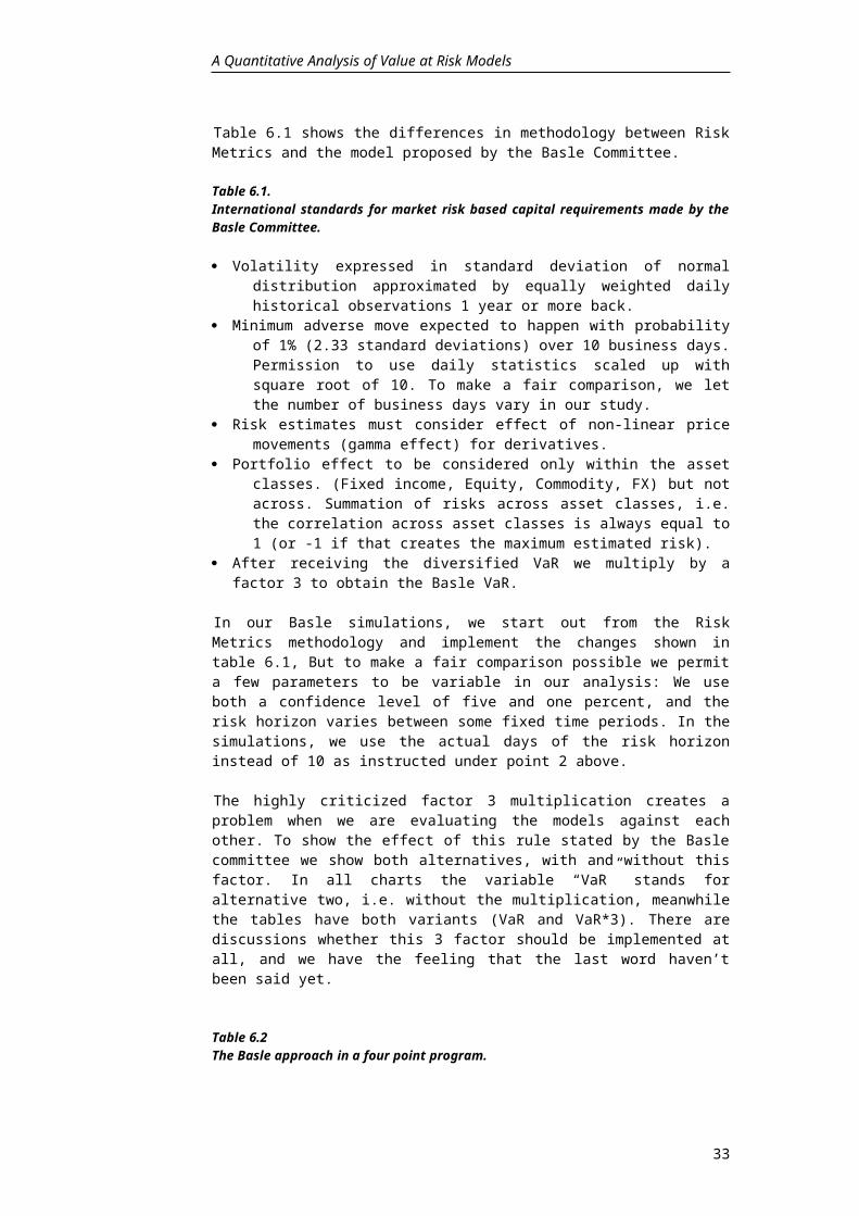
Table 6.1 shows the differences in methodology between Risk Metrics and the model proposed by the Basle Committee.

Table 6.1.International standards for market risk based capital requirements made by the Basle Committee.

· Volatility expressed in standard deviation of normal distribution approximated by equally weighted daily historical observations 1 year or more back.

· Minimum adverse move expected to happen with probability of 1% (2.33 standard deviations) over 10 business days. Permission to use daily statistics scaled up with square root of 10. To make a fair comparison, we let the number of business days vary in our study.

· Risk estimates must consider effect of non-linear price movements (gamma effect) for derivatives.

· Portfolio effect to be considered only within the asset classes. (Fixed income, Equity, Commodity, FX) but not across. Summation of risks across asset classes, i.e. the correlation across asset classes is always equal to 1 (or -1 if that creates the maximum estimated risk).

· After receiving the diversified VaR we multiply by a factor 3 to obtain the Basle VaR.

In our Basle simulations, we start out from the Risk Metrics methodology and implement the changes shown in table 6.1, But to make a fair comparison possible we permit a few parameters to be variable in our analysis: We use both a confidence level of five and one percent, and the risk horizon varies between some fixed time periods. In the simulations, we use the actual days of the risk horizon instead of 10 as instructed under point 2 above.

The highly criticized factor 3 multiplication creates a problem when we are evaluating the models against each other. To show the effect of this rule stated by the Basle committee we show both alternatives, with and without this factor. In all charts the variable “VaR” stands for alternative two, i.e. without the multiplication, meanwhile the tables have both variants (VaR and VaR*3). There are discussions whether this 3 factor should be implemented at all, and we have the feeling that the last word haven’t been said yet.

Table 6.2The Basle approach in a four point program.

1. Start off with the Risk Metrics methodology and then make the following adjustments to get the Basle VaR out of Risk Metrics.

2. Compute the volatilities and covariances with equal weights by daily observations 261 business days back.

3. Let the correlation coefficients that are related to instruments across asset classes equal 1. This means that the covariance among two instruments from different asset classes equals their volatilities multiplied by one another, i.e.

xyxy

x yxy xy x y

CovCov 1

4. Multiply the diversified VaR by three to obtain the Basle VaR.

22


7The Simulations

During the work with other first thesis we found that there were a lack of relevant mathematical investigations of the Value at Risk framework. What we were looking for was an analysis which captured the situation from the investment manager's point of view. If an investor implements a VaR model: does the VaR concept holds, i.e. can he or she rely on the confidence level? Does it work properly for all kinds of instruments?

In this analysis, we will try to give answers to these questions and to create an understanding for the most commonly used VaR methods. For every simulation we retrieve a figure representing something we call the 'actual VaR level', i.e. the number of occasions where the actual market risk exceeds the estimated VaR, expressed as a percentage of total observations. Hence, if the simulation is made on the 5% confidence level, a perfect match for the used method would be 5%. In this way, we are evaluating VaR using the definition the whole concept is built on.

7.1The 'Actual VaR Level'

To attain a proper 'actual VaR level', we need both the actual market risk and the estimated VaR (also referred to as ex-post and ex-ante VaR) from each model. To visualize the whole idea, consider figure 7.1 below. The bars show the day-to-day return of a T-bill portfolio and the fluctuating line indicates the estimated VaR.

Figure 7.1.The 'actual VaR level' concept. VaR estimation and day-to-day return for a T-bill portfolio consisting four foreign T-bills with 180 days to maturity (see portfolio 2 for further information). The risk horizon is one day and the confidence level 5%.

-2.50%

-2.00%

-1.50%

-1.00%

-0.50%

0.00%

0.50%

1.00%

1.50%

2.00%

2.50%

90 91 92 93 94 95 96

When the return bars pass below the VaR curve, the actual market risk exceeds the estimated VaR and the actual VaR level increases.

From this it is rather easy to construct a process chart over the calculation process. This four point program describes the core of our evaluation method:

23

1. Ex-ante: You are standing at time t. The only information available is the one for time £ t, i.e. you do not know anything about the future. Compute the estimated VaR for your portfolio for time t+trisk horizon according to each methodology.

2. Ex-post: The actual market risk receives from DNPV=NPV t+trisk horizon -NPVt. If we have lost money the DNPV (net present value of the difference) is negative.

3. Ex-post - Ex-ante: Calculate the difference between the actual risk and the estimated VaR, which is given by: Diff=DNPV+VaR. If the actual risk is larger than the estimated then Diff is negative, otherwise it is positive. We repeat the procedure 1-3 for each day in the period 900101-960710 and save the results.

4. Count how many times Diff is negative in our calculation period and divide by the total number of days. The answer is the 'actual VaR level'.

7.2Basic Assumptions for the Simulations

As mentioned in the previous section, we obviously need both the actual market risk and the estimated VaR from each model. A number of assumptions are stated to secure that the comparisons are consistent and that the implicit risk between the simulations is minimized.

The following assumptions are made to isolate market risk:

· There are 261 business days in a year.· The risk horizon is specified to one day, otherwise noted.· We use past financial data from 900101 to 960710, all together 1703 data points for

each risk factor.· To estimate past volatility for Risk Metrics and Monte Carlo Simulation, we use

exponential smoothing with a decay factor of 0.94 and 74 days. The BIS/Basle approach requires 261 days and an estimation based on equal weights. Both volatility estimates are presented for Historic Simulation.

· Due to the volatility, we have 1703-(74+1)=1628 days available for risk calculations with Risk Metrics and Monte Carlo Simulation, 1703-(261+1)=1441 days for BIS/Basle and 1703-(100+1)=1602 for Historic Simulation.

· All calculations are made after the market has closed. This means that we include data from the same day to estimate the risk for the next.

· The time to maturity for bills and options is constant, even though we compare two portfolios over a specified time horizon. This is rather unrealistic but we do not want to include any time value in our tests, only the market risk.

· Four different countries are chosen to describe the diversification effect, all equally weighted. These are DEM, JPY, USD and SEK. These countries are assumed to have efficient markets with good liquidity, to secure that the liquidity risk is as small as possible. This is also a representative sample from any Swedish investment portfolio.

· The weights are always 25% in each currency and are recalculated every day due to the fact that exchange rates vary.

We have used data for yield and exchange rates from the database company Datastream. Data for stocks and equity indices come from Reuters.

24


7.3Introducing the Simulations

First of all, the simulations are classified into six groups, all based on a hypothetical portfolio of instruments. Each portfolio has a section of its own and they are presented in the following order: FX-spot, T-bills, equity indices, stocks, currency options and equity options.

All four Value at Risk methodologies are applied to each portfolio, i.e. Historic Simulation, Risk Metrics, Monte Carlo Simulation and the VaR method proposed by the BIS and the Basle Committee.

In the entire analysis a one and a five percent confidence level (i.e. 1.65 and 2.33 standard deviations) is used to give an understanding of the tail distribution, and to provide a base for decision making on what level to use.

We also present the VaR curve for each methodology, which are quite characteristic as we will discover in a couple of pages. The VaR is expressed as a percentage of the total portfolio value. This creates a further knowledge in how the VaR models work and also brings a feeling for the different order of magnitude each instrument requires.

While using the measure 'actual VaR level' we permit the risk horizon to vary. This is important to investigate, since these models assume that the volatilities and correlations are constant over time. Due to the fact that the computer time for some models are quite significant, we had to determine what risk horizons to analyze. Since the Value at Risk concept mainly is designed for shorter risk windows, we put more weight the shorter the period. These are our twelve fixed risk horizons, all expressed in business days: 1, 3, 5, 10, 15, 20, 30, 50, 80, 130, 190, and 260 days.

The BIS/Basle approach is likely to follow the same pattern as Risk Metrics when different risk horizons are applicated, since it is based on the same theory. We have therefore excluded this section for BIS/Basle. The results along with the program code can however be retrieved by contacting the authors (this can be arranged for all the simulations).

25

7.4Portfolio 1 - Foreign Exchange

A position in a foreign currency (FX) is probably the most basic to simulate. In portfolio 1 we have equal amounts invested in DEM, JPY, SEK and USD. As we have seen in previous chapters, all VaR methods have radically different approaches, and below we will see the result in a graphical form. Figures 7.2a-d shows the risk estimation with a five percent confidence level using each VaR methodology. The VaR is expressed as percent of the total portfolio value.

Figure 7.2a Figure 7.2bRisk Metrics, VaR expressed as percent of total portfolio. Monte Carlo Simulation, VaR expressed as percent of

total portfolio

0.20%

0.40%

0.60%

0.80%

1.00%

1.20%

1.40%

apr-90 apr-91 apr-92 apr-93 apr-94 apr-95 apr-960.20%

0.40%

0.60%

0.80%

1.00%

1.20%

1.40%

1.60%

apr-90 apr-91 apr-92 apr-93 apr-94 apr-95 apr-96

Figure7.2c Figure 7.2dHistoric Simulation based on a worst Basle Method and Historic Simulation case scenario and a volatility estimation based on a volatility estimation withwith exponential smoothing equal weights

0.20%

0.40%

0.60%

0.80%

1.00%

1.20%

1.40%

1.60%

may-90 may -91 may -92 may -93 may -94 may -95 may -96

Worst CaseExponential Smoothing

0.20%

0.40%

0.60%

0.80%

1.00%

1.20%

1.40%

may-90 may -91 may -92 may -93 may -94 may -95 may -96

BasleEqual Weights

From the figures 7.2a-d we verify that the VaR is not at all a static tool, on the opposite it is highly dynamic at a degree that is stated by each methodology. During the period 1990-95 the Risk Metrics estimate fluctuates between an all time low of 0.4 percent to 1.4 percent of the total portfolio value (Fig 7.2a).

From the graphs we can tell the VaR methods' different characteristica. As shown by the graphs 7.2a,b and c, Risk Metrics and Historic Simulation with exponentially smoothed volatility follow almost perfectly the same pattern. This is, of course, due to the fact that they are all based on the exponential smoothing technique for the volatility estimation. Historic Simulation based on a worst case scenario of 100 days shows a more "skyline" characteristica, since a large temporary decrease in marketprice stays in

26


the 100-day-window for nearly five months. When the temporary down falls out of the window, there could be large drops in the Value at Risk estimation.

Historic Simulation and especially the Basle Method present less dramatic results than the others. Both models use volatility with equal weights which naturally slows down the dynamics and gives a more damped risk curve. The Basle approach only fluctuates within the range 0.7 to 0.9 percent of the portfolio value over a one day risk horizon.

From these graphs we also understand that it is both impossible and useless to say anything about their respective order of magnitude. This is a subject that has been highly debated in articles and often been an important part of the conclusions. For example, if we compare the Historic Simulation with a worst case approach to Risk Metrics (on the five percent confidence level), we find that there are periods when Risk Metrics estimate a risk that is twice as high as if using Historic Simulation, and periods when the relationship is the opposite. In 58.6 percent of the days from 900101 to 960710, the Historic Simulation (worst case) estimates a greater VaR than Risk Metrics. Hence it is almost impossible to draw any conclusions whether the other model will show greater or minor risk based on the information from the first. But, if we know that yesterday the other model created a greater VaR we could assume that possibly it will show the same relationship today, since this fluctuates periodically.

Now we have seen that the different Value at Risk models creates significantly different risk estimations. Can the theoretical confidence level hold in practice in the long run? Table 7.1 shows how often the actual risk exceeds the estimated VaR.

Table 7.1Actual VaR levels for different VaR methods on a equally weighted currency portfolio consisting DEM, JPY, SEK and USD (one day risk horizon).

5%-level 1%-level

Historic Simulationworst case : 4.81% 1.31%stdev Risk Metrics : 4.81% 2.06%stdev equal weights : 4.37% 1.81%

Risk Metrics : 4.79% 2.09%

BIS / BasleVaR : 4.65% 1.80%VaR*3 : 0.00% 0.00%

Monte Carlo Simulation : 5.46% 2.09%

The first and most important thing to notice is that all methods work very well, particularly on the five percent level. The only method that slightly underestimates the market risk is the Monte Carlo Simulation where the estimated limit was exceeded in 5.46 percent of the 1628 business days, simply 0.46 percent higher than desired.

On the one percent confidence level, we can easily identify another important and clear pattern : the one percent level appears to be closer to the two percent level. This is not at all surprising. Since most financial data show leptokurtosis12, i.e. high peaks and fat tails, the fat tails create more negative outliers than the Gaussian curve implicates. Therefore we have a larger amount of days where the actual risk is underestimated and we get a higher actual Value at Risk level. Historic Simulation based on a worst case scenario is the method that creates the best risk calculation in this matter, but it is also the only model that does not assume normality.

12 See for instance Pfaffenberger/Patterson, “ Statistical Methods for Business and Economics”.

27

The conclusion is that even though the VaR methods creates significantly different risk estimates all our methods corresponds amazingly well to the intentioned risk level, given our portfolio of currencies. As far as we are aware of the problems with leptokurtosis, VaR should be a reliable tool in every firms currency risk management.

One of the most controversial issues around Value at Risk methods is that the volatilities and covariances are not stable over time. This indicates also our calculations. In figure 7.3 we present the standard deviation for the exchange rate DEM/USD and the correlation coefficient for DEM/SEK based on exponential smoothing and equal weights respectively.

Figure 7.3a Figure 7.3bStandard deviation for DEM/USD with Correlation between DEM/SEK withexponential smoothing and equal weights exponential smoothing and equal weights(261days) (261 days)

0.20%

0.40%

0.60%

0.80%

1.00%

1.20%

1.40%


Equal WeightsExponential Smoothing

0.0

0.1

0.2

0.3

0.4

0.5

0.6

0.7

0.8

0.9

1.0

may-90 may-91 may-92 may-93 may-94 may-95 may-96

Equal WeightsExponential Smoothing

Note here that the DEM and the SEK were almost perfectly correlated during 1991 but later the coefficient has decreased to nearly zero. Even the standard deviation varies up to five times its value during the period.

Since the variance and the correlation are not stable we can not be sure that the VaR estimate will work over a long risk horizon. Until now all our calculations have been computed with a one day risk period. Now we extend this risk horizon to be variable and figure 7.4 indicates how often the actual market risk is greater than the estimated for our VaR methodologies for different investment periods.

Risk Metrics and the Basle approach use the square root of time rule, i.e. that you only multiply the daily VaR with the square root of time expressed in days. This is not possible in the Monte Carlo Simulation. Instead we multiply the covariance matrix in the beginning of the calculation process. In Historic Simulation you only change the time step in the NPV difference13. Therefore, Historic Simulation does not depend on the assumption that derives the square root of time rule, i.e. financial data are not serially correlated.

First, consider figure 7.4a,b. Risk Metrics shows a slowly decreasing actual VaR level over time, i.e. the longer the risk horizon the more the actual VaR level decreases. During the first half year on the five percent level, the actual VaR fluctuates around the five percent level but with a risk horizon of more than 160 days the VaR exaggerates the estimate.

13 See equation 3.1

28


Figure 7.4a,b Actual VaR levels for different risk horizons.

0%

1%

2%

3%

4%

5%

6%

1 3 5 10 15 20 30 50 80 130 190 260

Risk Metrics 5%Risk Metrics 1%

0%

1%

2%

3%

4%

5%

6%

1 3 5 10 15 20 30 50 80 130 190 260

Monte Carlo 5%Monte Carlo 1%

a) Risk Metrics b) Monte Carlo Simulation

We observe the same pattern on the one percent level, with the exception that the VaR starts at two percent and decreases down to one during the first 130 days. After that, with a risk horizon of more than a half year, the estimated VaR almost never exceeds the actual market risk. The Monte Carlo Simulation in figure 7.4b creates a similar curve. Hence, as long as we use exponential smoothing for the volatility estimation, the Risk Metrics and the Monte Carlo Simulation follow each other in their VaR estimates.

For Historic Simulation there is one very important thing to notice. Consider figure 7.4c and d.

Figure 7.4 c,dActual VaR levels for different risk horizons.

0%

5%

10%

15%

20%

25%

30%

1 3 5 10 15 20 30 50 80 130 190 260

Exponential SmoothingEqual WeightsWorst Case

0%

5%

10%

15%

20%

25%

30%

1 3 5 10 15 20 30 50 80 130 190 260


c) Historic Simulation, 5%-level d) Historic Simulation, 1%-level

As the graphs above indicate, the worst case scenario alternative does not work at all for longer risk horizons! In a five month risk window, the actual risk exceeds the estimated in one day out of four. Even the alternative based on exponentially smoothed volatility tends to increase above the recommended theoretical level for risk horizons between one and three months, but gives better result than the worst case scenario. The last alternative, which is based on equally weighted volatility, resembles the Risk Metrics and the Monte Carlo Simulations and functions very well.

29

7.5Portfolio 2 - Treasury Bills

The second portfolio consists exclusively of four foreign Treasury Bills (T-bills). They are all equally weighted in that sense that the proprietor obtain an equal amount of money expressed in dollars at the expiration date. They have a time to maturity of 180 days and the T-bills are invested in DEM, JPY, SEK and USD.

As we have seen in the previous section, all VaR methods create radically different risk curves, mainly depending on the implicit volatility estimation model. The actual VaR curves for our T-bill portfolio are printed in figure ?4? below. The risk is expressed in percent of the total portfolio value and the risk horizon is one day.

Figure 7.5a,bActual VaR curves for a portfolio consisting T-bills with a maturity of 180 days during the period 1991-92.

0.20%

0.40%

0.60%

0.80%

1.00%

1.20%

1.40%

1.60%

1.80%


BasleWorst CaseRisk Metrics

0.20%

0.40%

0.60%

0.80%

1.00%

1.20%

1.40%

1.60%

1.80%

2.00%

maj-90 maj-91 maj-92 maj-93 maj-94 maj-95 maj-96

Equal Weights

Monte Carlo

Exponential Smoothing

a) b)

From figure 7.5a we can clearly verify that the worst case scenario of Historic Simulation shows a higher estimated VaR than Risk Metrics and therefore it probably will have a lower actual VaR level (see table 7.2 below). The Basle approach is again the least dynamic device which only fluctuates within 0.1 percent. Compare Basle to the Historic Simulation based on exponentially smoothed volatility, where the risk estimate moves between 0,.8 and 2.0 percent of the portfolio value. Also note that the Monte Carlo Simulation computes the lowest VaR estimate in general of all our methods.

Since the Value at Risk concept is a statistical estimate it is important to compute how often the actual market risk is higher than the estimated. To investigate this and to see how all the methods function in the long run we calculate our own measure "the actual VaR level",

30


Table 7.2Actual VaR levels for different VaR methods on a equally weighted T-bill portfolio consisting DEM, JPY, SEK and USD and a time to maturity of 180 days. The risk horizon is one day.

5%-level 1%-level



BIS / BasleVaR : 4.58% 1.67%VaR*3 : 0.00% 0.00%


This table is similar to the corresponding currency portfolio. For the T-bill position we can establish that all VaR models works satisfactionally, especially on a five percent confidence level. Monte Carlo Simulation is the only method that underestimates the actual market risk.

We also notice that the worst case alternative of the Historic Simulation is the best predictor on the one percent confidence level. All models except from the worst case of Historic Simulation are based on the normality assumption, hence the actual VaR level is closer to two than to one percent.

The VaR analysis of portfolio 2 reveals quite similar characteristics for different risk horizons as portfolio 1. For our T-bill position there arises a rather peculiar situation. Since we are only interested in analyzing the market risk versus the estimated Value at Risk, we try to isolate the market risk as much as possible. Therefore we do not calculate any time value for bills or bonds, i.e. we hold the maturity time for our bills constant (for example 180) even though we compare the portfolio value over a risk horizon of a couple days. The odd situation is that the maturity time for the bill is 180 days and the risk horizon is maximum 260, hence the risk horizon exceeds the maturity time with 80 days. But this is just a theoretical and technical trick that has no influence on the analysis result.

In figure 7.6a and b, we clearly identify the same pattern as for portfolio 1. Risk Metrics demonstrates a slowly decreasing actual Value at Risk curve over time, which means that the estimated risk gets higher and higher compared to the actual market risk. After about more than four or five months the estimated VaR is so large that it rarely ever underestimates the actual risk.

31

Figure 7.6a,b Actual VaR levels for different risk horizons on a T-bill portfolio.

0%

1%

2%

3%

4%

5%

6%

1 3 5 10 15 20 30 50 80 130 190 260


0%

1%

2%

3%

4%

5%

6%

1 3 5 10 15 20 30 50 80 130 190 260



Monte Carlo Simulation creates almost the same actual VaR graph as Risk Metrics. For both methods it takes about 30 days for the actual one percent VaR level to reach the theoretical one percent confidence level.

As for the currency portfolio, we must warn everyone not to the use the worst case scenario version of the Historical Simulation model, particularly for longer risk periods!

Figure 7.6c,d Actual VaR levels for different risk horizons on a T-bill portfolio.

0%

5%

10%

15%

20%

25%

30%

1 3 5 10 15 20 30 50 80 130 190 260


0%

5%

10%

15%

20%

25%

30%

1 3 5 10 15 20 30 50 80 130 190 260


a) Historic Simulation, 5%-level b) Historic Simulation, 1%-level

The worst case Historic Simulation creates a disastrous result on the actual VaR level. For a risk horizon of two weeks or more the estimated Value at Risk is not at all to trust! Even this time, as for portfolio 1, we have an increase in the exponentially based alternative for a risk window between one and three months. This is a rather strange phenomenon and we cannot explain it. The only version of Historical Simulation to rely on is the one with volatility estimates calculated with equal weights.

32


7.6Portfolio 3 - Stock Indices

The third portfolio consists of four different stock indices. We have chosen wide indices since they represent a well diversified portfolio in each market.

Our stock index portfolio includes the following indices:

· DAX 100 performance index· TOKYO SE (Topix) index· Affarsvarldens weighted all shares index (AFGX)· Standard and Poor 500 Composite index (S&P 500)

Most of them have had a positive performance during the nineties (figure 7.7). The only exception from this is the Japanese index that has decreased with 31 percent.

Figure 7.7Stock index performance in percent from DAX 100, TOPIX, Affarsvarlden and S&P 500.

30

50

70

90

110

130

150

170

190

1990 1991 1992 1993 1994 1995 1996

S&P 500TopixAFGXDAX

If we normalize the index values at 1/1-90, we find that the Standard and Poor 500 has had the best performance until 10/7-96. Even the Swedish and the German indices have increased about forty or fifty percent. Intuitively we probably consider the stock market to be more volatile than the interest market, an opinion which is verified in figure 7.7 below.

Figure 7.8a,bActual VaR curves for a portfolio consisting stock indices with a risk horizon of one day with a five percent confidence level.

0.20%

0.70%

1.20%

1.70%

2.20%

2.70%

3.20%

3.70%

4.20%


Risk MetricsBasleWorst Case

0.20%

0.70%

1.20%

1.70%

2.20%

2.70%

3.20%

3.70%


Equally Weighed


Monte Carlo

a) b)

33

If we recall the corresponding figures from the currency or the T-bill portfolios we remember that the Risk Metrics risk was fluctuating around 0.8% with a maximum peak of 1.7%. Compare that to figure 7.8a where Risk Metrics has a maximum of 3.1% and an average level of 1.2 percent. All VaR methodologies have definitely both a higher medium level and peaks for stock indices than for currencies.

For stock indices we clearly detect that the Basel VaR has increased to about 2.2% in general. This is not surprising since the Basle methodology does not allow any cross correlations among asset classes and accordingly the correlation coefficient is set constant to 1 (or -1) between the currencies and the stock indices. For our stock index portfolio we estimate the Basle VaR to be twice as high as for the other models. We emphasize here that we do not multiply the Basle VaR with three for the linear instruments which is established in the Basle committee proposal, since if we did the actual risk would never be even close to the estimated VaR.

We are also interested in how our models work in the long run. As usual we measure this by calculating how often the market risk exceeds the estimated Value at Risk. You find the Actual VaR levels for the stock index portfolio in the table below.

Table 7.3Actual VaR levels for different VaR methods on an equally weighted stock index portfolio based on a one day risk horizon.

5%-level 1%-level



BIS / BasleVaR : 0.63% 0.14%VaR*3 : 0.00% 0.00%


Even this time we verify that most models behave very well. The increased risk estimation for the Basle methodology is indicated by the extremely low Actual VaR levels, 0.63% on the five percent confidence level and 0.14 on the one percent level. This constraint creates a too strong risk level which undermines the model, even without the "multiply with three" paragraph. We also recognize the leptokurtosis behavior from the stock indices that makes the one percent confidence level to be 2 percent in practice.

34


Since the volatilities and correlations vary over time we are interested in the VaR methods' behavior when the risk horizon increases. First, consider figure 7.9a,b below. Risk Metrics produces a slowly decreasing actual VaR level over time. For a risk horizon shorter than 130 days the value mainly fluctuates around 4-5 percent with a five percent confidence interval. After that, for a risk period longer than a half year, the actual VaR level falls down to 1% which indicates that the estimated VaR is too high. On the one percent confidence level, Risk Metrics is almost stable at 2 percent again for the first five months, after that the actual VaR level goes down to zero. As indicated in portfolio 1 to 3, this risk horizon is a crucial one. If exceeded the actual VaR falls drastically. As we have seen for the previous portfolios, the Monte Carlo Simulation follows Risk Metrics almost identically, and that relationship seems to hold even for stock indices. Figure 7.9a,b Actual VaR levels for different risk horizons on a stock index portfolio.

0%

1%

2%

3%

4%

5%

6%

7%

1 3 5 10 15 20 30 50 80 130 190 260


0%

1%

2%

3%

4%

5%

6%

7%

1 3 5 10 15 20 30 50 80 130 190 260



Historic Simulation with the worst case scenario assumption does not give satisfactionally results for longer risk windows. Figure 7.9 c and d verifies the issue.

Figure 7.9c,d Actual VaR levels for different risk horizons on a stock index portfolio.

0%

2%

4%

6%

8%

10%

12%

14%

16%

18%

1 3 5 10 15 20 30 50 80 130 190 260


0%

2%

4%

6%

8%

10%

12%

14%

1 3 5 10 15 20 30 50 80 130 190 260


c) Historic Simulation 5%-level b) Historic Simulation 1%-level

The other alternatives of Historic Simulation exhibit a more stable result. They fluctuate constantly around 4 percent on the 1.65 standard deviation confidence. Even here we recognize the influences from leptokurtosis since the actual VaR level stays closer to two percent for 2.33 standard deviations than to one percent.

35

7.7Portfolio 4 - Equity

Our fourth portfolio consists of individual stocks, one stock from each market. We have chosen them "randomly", i.e. we have tried to pick them from different lines of business and with different performance during the period 1990 to 1996. This means of course that we would have received another risk profile and performance from our portfolio if we had chosen a different set of stocks. We are aware of that but anyway we hope that our portfolio will highlight the problems surrounding VaR with stocks. We must also emphasize here that we have not made any research to get a portfolio with these characteristics, we have only put together our first "random" choice.

Our stock portfolio consists of:

· Deutsche Bank, which is registered at (DAX).· Mitsumi Electrics, Tokyo· L M Ericsson, Stockholm· The Coca Cola Company, NYSE

All stocks are noted in their local currency which of course generates a currency risk as well as the stock specific risk. Figure 7.10 displays the normalized performance of each stock in their local market.

Figure 7.10Stock performance in their local market.

50

100

150

200

250

300

350

400

450

500

1990 1991 1992 1993 1994 1995 1996

Coca Cola, NYSEMitsumi Electrics, TokyoEricsson, StockholmDeutsche Bank, Frankfurt

The graph above exhibits that the Swedish and the American stocks have had an impressive growth through out the nineties, while the Japanese and particularly the German stock have been less successful. As we have seen, both stocks and stock indices have a drift which makes them grow over time. The statistical theory behind the VaR methods is based upon the assumption that the drift equals zero which adds another disturbing factor to the concept.

As for stock indices we find that the estimated VaR for stocks is substantially higher than for FX or T-bills, naturally due to the larger volatility in the stock market. Most models produce a VaR estimation of 1.0-1.5 % of the portfolio value which is twice or three times as much as for the FX portfolio.

36


Figure 7.11a,bActual VaR curves for a portfolio consisting different stocks with a risk horizon of one day and a five percent confidence level.

0.20%

1.20%

2.20%

3.20%

4.20%

5.20%

6.20%


Risk Metrics

Basle

Worst Case

0.50%

1.50%

2.50%

3.50%

4.50%

5.50%

6.50%


Equal Weights


Monte Carlo

a) b)

The most interesting feature is again the Basle approach, which starts at 4.0 % and slowly goes down to 3.0%. The fact that the correlation across asset classes is always set to 1 creates this sharp increase in VaR. Another important thing to pay attention to is that Risk Metrics with its beta transformation computes the far lowest VaR of all. It is verified that it was too low in table 7.4. A model which creates an actual VaR level of 11.04% on the five percent level is not approved. On the one percent confidence level, Risk Metrics creates an even worse result: 5.31% !

Table 7.4Actual VaR levels for different VaR methods on an equally weighted stock portfolio based on a one day risk horizon.

5%-level 1%-level


Risk Metrics (incl. CAPM assumption) : 11.04% 5.31% (excl. CAPM assumption) : 3.70% 1.30%

BIS / BasleVaR : 0.77% 0.14%VaR*3 : 0.00% 0.00%


This problem arises because JP Morgan wants to daily update the volatilities and the correlations on the Internet. Obviously it is impossible to compute the correlations between every existing equity in the world. Therefore, JP Morgan uses a version of the Capital Asset Pricing Model to reduce the number correlations necessary to include only the stock indices as risk factors.

But this CAPM transformation does not work properly in this case, probably because our selected stocks do not behave like their corresponding stock indices. To completely investigate the Risk Metrics methodology we extend the analysis further more. If we assume that we create the correlations between each of our stocks and currencies ourselves, would that produce a better estimation than Risk Metrics with the CAPM

37

assumption? Table 7.4 above presents the answer to 3.70% with five percent confidence and 1.73% on the one percent level.

Obviously the Risk Metrics methodology holds for stocks in that sense that the variance / covariance approach works very well. But we must emphasize that the CAPM transformation is nothing to rely on for small stock portfolios that doesnÕt behave in the same way as the stock index does. Our test portfolio is of course rather unusual with one stock each from four different countries, but it clearly highlights the problems with Risk MetricsÕ CAPM transformation. Therefore, we recommend private investors or financial firms with an investment portfolio which differ from the index portfolio that they should be aware of this and try to calculate the correlations themselves.

How do these VaR models conduct for variable risk horizons? Most of them behave the way we anticipate from our experience based on the previous portfolios. Risk Metrics and Monte Carlo Simulation decreases more rapidly than before but they show on the whole the same pattern.

Figure 7.12a,b Actual VaR levels for different risk horizons for a portfolio consisting stocks.

0%

2%

4%

6%

8%

10%

12%

14%

1 3 5 10 15 20 30 50 80 130 190 260

Risk Metrics 5% (CAPM)Risk Metrics 1% (CAPM)Risk Metrics 5%Risk Metrics 1%

0%

1%

2%

3%

4%

5%

6%

1 3 5 10 15 20 30 50 80 130 190 260



Even the Historic Simulation displays the usual graphs for the worst case scenario, which means that it works terribly for longer risk windows than a few days. But all of the Historic models exhibit an increased actual VaR level for three days to two weeks risk horizon, both on the five and the one percent confidence level. This is rather strange and we do not have an explanation for the phenomenon.

Figure 7.12c,d Actual VaR levels for different risk horizons for a portfolio consisting stocks.

0%

5%

10%

15%

20%

25%

30%

1 3 5 10 15 20 30 50 80 130 190 260

Worst CaseExponential SmoothingEqual Weights

0%

5%

10%

15%

20%

25%

1 3 5 10 15 20 30 50 80 130 190 260

Worst CaseExponential SmoothingEqual Weights


38


7.8Portfolio 5 - Currency Options

The fifth and sixth portfolio are constructed to display the complex risk dynamics for options. First, we examine a portfolio consisting three currency options, three calls which are issued in the US and give the proprietor the right to purchase DEM, JPY and SEK respectively, with an expiration date 180 days a head. Initially, all instruments are pari options, which means that the expiration price and the current market price are equal.

To evaluate the portfolio we need an option pricing model which includes both the delta and gamma values.

The formulas for pricing currency options follows:

(7.1) c Se rfT N d1 Xe rTN d2 p Xe rTN d2 Se rf TN d1

where

dS X r rf T

T1

2 2

ln

and

dS X r rf T

Td T2

2

1

2

ln

The variables are· c = the price of a European call· p = the price of a European put· S = the stock price· X = the strike price· r = the risk-free interest rate· rf= The risk-free in the foreign interest rate· T = time to expiration· = the volatility of the underlying stock price

Both the domestic interest rate, r, and the foreign interest rate, r f, are assumed to be constant and the same for all maturities. Note that put and call options on a currency are symmetrical in that a put option to sell currency A for currency B at an exercise price X is the same as a call option to buy B with A at 1/X.

For Risk Metrics and the Basel approach we also need the delta and gamma functions:

(7.2) e rf TN d1 for call options

e N dr Tf1 1 for put options

N' d1 erfT

S T for both call and put options

where d1, d2 and N(d1) are given by (7.1) and (7.3) respectively.The only problem with applying equations (7.1) and (7.2) is the computation of the cumulative normal distribution function, N(x). The function can be evaluated using a

39

polynomial approximation. We utilize an approximation14 that is fairly simple, but even though it has a sufficient accuracy.

(7.3) N x a k a k a k N x 1 1 22

33 ' when x³0

N x N x 1 when x<0

where k = 1 / (1 + x ) = 0.33267 a1 = 0.4361836 a2 = - 0.1201676 a3 = 0.9372980

and

N x e x' 12

2 2

This provides values for N(x) that are always accurate to 0.0002 which is sufficient enough for our purposes.

As mentioned in the theory sections, each VaR methodology show radically different approaches to derivatives which of course results in different VaR estimates. Figure 7.13 below, exhibits the VaR curves for each methodology. In our analysis, we include both the delta and the delta/gamma approximation for Risk Metrics, but only delta/gamma for the Basle approach. The Historic Simulation and the Monte Carlo method require only the option pricing formula in their calculation processes.

There has been an intense discussion surrounding Risk Metrics and options. In our previous thesis we analyzed the option mathematics and found that the most sensitive variable in the risk estimation process is the proportion between the strike price X and the spot rate S. We have called this relationship the lambda ratio which follows :

(7.4) S / X

This entails that an equity call for instance is in the money as long as the is larger than one. Initially, we have set =1.00 which means that the calls included in portfolio five are always pari options. Later in the evaluation we let the lambda to be variable which will cause interesting effects on the actual VaR level. But first, consider the estimated VaR curves for each model with =1.

14 The approximation for N(x) belongs to ”Introduction to futures and options market” by Mr John Hull, page 269

40


Figure 7.13a,bThe estimated VaR curves for our methodologies with a risk window of one day and lambda set to 1.

0%

5%

10%

15%

20%

25%

30%

35%

40%

45%

jun-90 jun-91 jun-92 jun-93 jun-94 jun-95 jun-96


0%

5%

10%

15%

20%

25%

30%

35%

jun-90 jun-91 jun-92 jun-93 jun-94 jun-95 jun-96

Exponential SmoothingMonte CarloEqual Weights

a) b)

As displayed in figure 7.13, the estimated risk levels are substantially higher for options than for the linear instruments presented in portfolio one to four. We are now facing a one-day-risk of about 25 percent for our currency options, compared to 1 percent for the underlying currencies alone.

As usual, we investigate how the derivatives behave over the period 1990-96 by evaluating the Actual VaR levels.

Table 7.5Actual VaR levels for different VaR methods on a portfolio consisting currency calls in DEM, JPY and SEK, all related to USD in the American market (one day risk horizon and =1).

5%-level 1%-levelHistoric Simulation

worst case : 5.17% 1.22%stdev Risk Metrics : 4.35% 1.43%stdev equal weights : 4.08% 0.75%

Risk Metricsdelta : 3.88% 1.15%delta / gamma : 2.74% 0.70%

BIS / BasleVaR : 2.57% 0.49%VaR*3 : 0.00% 0.00%


As table 7.5 above indicates, all methods perform all right, even if the differences between them are more distinguishable than usual. The most apparent thing to pay attention to is for most models the one percent confidence level works better here, i.e. are closer to 1, than for linear instruments. Risk MetricsÕ two versions differ slightly in their actual VaR levels. The two to three percent higher estimated VaR for the delta/gamma alternative that we observed previously leads to a one percent lower actual VaR.

Until now all calls have been pari options. But what happens if the options are in or out of the money, i.e. 1.00? To investigate each VaR methodology's sensitivity to different proportions between strike and spot price we permit the lambda to vary

41

between 50 and 150 percent. The relationship between and the actual VaR level is presented in figure 7.14. Still, the risk window is one day.

Figure 7.14a,bActual VaR levels for different =S/X where lambda varies between 50 and 150 percent. The risk horizon is one day.

0%

1%

2%

3%

4%

5%

6%

0.5 0.6 0.7 0.8 0.9 1 1.1 1.2 1.3 1.4 1.5

Delta 5%Delta/Gamma 5%Delta 1%Delta/Gamma 1%

0%

1%

2%

3%

4%

5%

6%

0.5 0.6 0.7 0.8 0.9 1 1.1 1.2 1.3 1.4 1.5


a) Risk Metrics, delta and delta/gamma b) Monte Carlo Simulation

In figure 7.14a above we clearly identify the famous problems about Risk Metrics and derivatives. When the options are out of the money, i.e. =92%, we obtain an actual VaR level from Risk Metrics delta and delta/gamma versions of 35 and 32 percent respectively. This is a terrible result and could create a financial disaster. That means that an investment manager that relies on JP Morgan's concept faces an actual market risk which is higher than the estimated every third day, while at the same time he thinks it occurs only one day out of twenty. When the spot rate is larger than the strike price, the scenario is the opposite which entails a zero actual VaR level. Overestimation is naturally better than underestimation but an estimated VaR which is too high results probably in bad performance and a very small freedom of action.

Gamma does not improve the result materially. An actual VaR level that has sank from 35 to 32 percent doesn't make anyone satisfied and the difference decreases only slowly. This pattern also appears for the one percent confidence interval.

But worst of all, this is not at all an impossible situation. A spot rate which is eight percent lower than the strike price is highly plausible to arise in the everyday market. This analysis reveals that Risk Metrics is not a tool to trust 15 and therefore, we recommend the investor that has a portfolio consisting non-linear instruments to avoid the methodology.

But fortunately there are models that are less influenced from the spot/strike price relationship. Monte Carlo Simulation in figure 7.14b appears to be almost independent of it and displays an impressive reliability. But the approach has its drawbacks too. Monte Carlo Simulation is highly computer intensive and the calculation time increases fast with the number of instruments involved. We have used SPARC 5 computers from SUN Microsystems and for each actual VaR level value in figure 7.14b the calculation time is 10 to 11 hours. As a comparison, Risk Metrics requires three minutes for the same portfolio which explains the attention it has gained the last years.

Historic Simulation places itself in the middle in our computer time competition. Each actual VaR level evaluation takes about three hours. Historic Simulation also places itself in the middle regarding the lambda effect.

Figure 7.14c,d

15 JP Morgan has updated their methodology in this area. We have worked with the model presented in their 3rd edition of “Risk Metrics Technical document”.

42


Actual VaR levels for different =S/X where lambda varies between 50 and 150 percent. The risk horizon is one day.

0%

2%

4%

6%

8%

10%

12%

0.5 0.6 0.7 0.8 0.9 1 1.1 1.2 1.3 1.4 1.5


0%

1%

2%

3%

4%

5%

0.5 0.6 0.7 0.8 0.9 1 1.1 1.2 1.3 1.4 1.5


a) Historic Simulation, 5%-level b) Historic Simulation, 1%-level

As indicated in figure 7.14 above, Historic Simulation (exponential smoothing) suffers from the same problem as Risk Metrics. Those two alternatives which apply the normal assumption, tend to decrease by roughly 3.5% with a five percent confidence and 1.5% for the 1 percent, with the exception that the alternative based on equal weighted volatility turns and increases when lambda overruns 120%. Under the circumstances this is sufficient enough but not impressive and not completely reliable. On the contrary, the worst case approach seems to be almost unaffected by the variable in the region close to =1,00, but increases fast for options far in the money.

Now, let's return to a our primary portfolio which held pari options, i.e. =1. We permit the risk window to vary and analyze the resulting diagrams.

Figure 7.15a,bActual VaR levels for different risk horizons (=1).

0.0%

0.5%

1.0%

1.5%

2.0%

2.5%

3.0%

3.5%

4.0%

1 3 5 10 15 20 30 50 80 130 190 260

Risk Metrics Delta 5%Risk Metrics Delta/Gamma 5%Risk Metrics Delta 1%Risk Metrics Delta/Gamma 1%

0%

1%

2%

3%

4%

5%

6%

1 3 5 10 15 20 30 50 80 130 190 260



Risk Metrics' VaR obviously decreases very fast with the risk horizon. This is quite natural since the one-day-VaR is as high as 25% of portfolio value. Using the square root of time rule16 we get a VaR of 125% after only 25 five days. From figure 7.15a we also find that the delta/gamma alternative, which created a just slightly higher VaR, decreases significantly faster than the delta approach. This depends on the fact that you multiply the gamma with the volatility estimate over the risk window, a volatility which naturally increases for a longer risk horizon.

As for the other models, we recognize the pattern for Historic Simulation as well.

Figure 7.15c,d

16 See equation 4.6.

43

Actual VaR levels for different risk horizons (=1).

0%

2%

4%

6%

8%

10%

12%

14%

16%

1 3 5 10 15 20 30 50 80 130 190 260


0%

1%

2%

3%

4%

5%

6%

1 3 5 10 15 20 30 50 80 130 190 260



Unfortunately, the worst case scenario gets off the track as usual. Although it appears to be the best alternative regarding the lambda effect, it evidently doesn't hold for longer risk windows than one or two weeks. The versions using standard deviation exhibit a slowly declining curve which better imitate the behavior of the underlying instrument.

44


7.9Portfolio 6 - Equity Options

The sixth portfolio contains of four equity calls, which give the proprietor the right to purchase one share of the underlying equity at a date 180 days ahead. To make a comparison possible we use the same underlying stocks as in portfolio 4, namely

¥ Deutsche Bank, which is registered at Frankfurt¥ Mitsumi Electrics, Tokyo¥ L M Ericsson, Stockholm¥ The Coca Cola Company, NYSE

Each of them are issued in their own market. Therefore, the corresponding option values are expressed in their local currency which give rise to currency risks. But to compute the value of the calls we need an option pricing model.

The pricing formulas for the prices of European calls and puts on nondividend-paying stocks17 are

(7.4) c SN d1 Xe rTN d2 (7.5) p Xe rTN d2 SN d1

where

d1 ln S X r 2 2 T

T

d2 ln S X r 2 2 T

Td1 T

The variables are:

· c = the price of a European call· p = the price of a European put· S = the stock price· X = the strike price· r = the risk-free interest rate· T = time to expiration· = the volatility of the underlying stock price

To the Risk Metrics and Basel methods, we also need formulas for delta and gamma. For European call and put options on a nondividend-paying stock, it can be shown that

(7.6) N d1 for calls

N d1 1 for puts

N' d1 S T

for both calls and puts

As for the previous portfolio, we use the approximation for the cumulative normal distribution function N(x) from equation (7.3) .

17 The pricing furmulas are taken from ÓIntroduction to futures and options marketÓ by Mr John Hull, page 267

45

Similar to portfolio 4, we have extended the analysis to contain two versions of Risk Metrics: one that is based upon the principles of the Capital Asset Pricing Model (CAPM) and one that includes correlations among the stocks and the currencies. Hence, all calculations with this derivative portfolio can easily be compared to the corresponding one solely including the underlying equity.

To make a fair comparison possible between the previous portfolio and this one, we will follow the same procedure. Therefore, initially, we set the proportion lambda between the strike price X and the spot rate S to equal 1. First, consider the VaR curves for the different methodologies in Figure 7.16.

Figure 7.16a,bVaR expressed as percent of portfolio value for the equity pari option portfolio (one day risk horizon, =S/X=1).

0%

5%

10%

15%

20%

25%

30%

35%

jun-90 jun-91 jun-92 jun-93 jun-94 jun-95


0%

5%

10%

15%

20%

25%

jun-90 jun-91 jun-92 jun-93 jun-94 jun-95

Exponential SmoothingMonte Carlo

Equal Weights

a) b)

Again, we find that the VaR for options is fluctuating around 20 percent compared to the underlying instrument's VaR of two percent. The most important feature is that there is only a marginally difference between Risk Metrics'Êdelta and delta/gamma approaches.

Table 7.6Actual VaR levels for different VaR methods on a portfolio consisting four equity options (one day risk horizon and =1).

5%-level 1%-levelHistoric Simulation

worst case : 4.99% 0.89%stdev Risk Metrics : 4.30% 1.02%stdev equal weights : 3.42% 0.75%

Risk Metrics incl. CAPM assumption

delta : 5.88% 1.92%delta / gamma : 5.88% 1.92%

without CAPM assumptiondelta : 2.30% 0.51%delta / gamma : 2.30% 0.51%

BIS / BasleVaR : 0.21% 0.07%VaR*3 : 0.00% 0.00%


46


First of all, including gamma does not have any impact at all on Risk Metrics' VaR estimate. We also notice that Monte Carlo and Historic Simulation are close both to the five and to the one percent confidence limit. On the other hand, Risk Metrics and particularly the BIS/Basle approach are significantly lower than their explicit confidence level. If we compute the VaR according to the Basle proposal we would have a VaR estimate which always is larger than the actual market risk.

Another thing to take under consideration is the volatility estimate used in the option pricing formulas. A rule of thumb is to use equal weighted volatility estimate over the same period as the expiration time of the option. In our portfolio, T is set to 180 days which is equivalent to 130 business days. After that we multiply the volatility with the square root of 261 days to obtain the annual volatility for the option. This is very important, since if we apply an exponentially smoothed variance instead, we will receive a very different and less adequate VaR estimate.

Up to this point all options have been set to pari, i.e. =S/X=1. Now we will analyze the effect from having in-the-money, and out-of-the money options by varying . The risk horizon continues to be one day.

Figure 7.17a,bActual VaR levels for different =S/X where lambda varies between 50 and 150 percent. The risk horizon is one day.

0%

2%

4%

6%

8%

10%

12%

0.5 0.6 0.7 0.8 0.9 1 1.1 1.2 1.3 1.4 1.5

Delta/Gamma 5% (CAPM)Delta/Gamma 5%Delta/Gamma 1% (CAPM)Delta/Gamma 1%

0%

1%

2%

3%

4%

5%

6%

0.5 0.6 0.7 0.8 0.9 1 1.1 1.2 1.3 1.4 1.5


a) Risk Metrics, incl. and excl. CAPM b) Monte Carlo Simulation

Including gamma does not have any impact at all on Risk Metrics’ VaR estimate, since the gamma term is always too small compared to delta. The chart also indicates what we have observed in portfolio four; that Risk Metrics with the CAPM transformation con create strange phenomenons in the risk estimation. Our own alternative of Risk Metrics with computed correlations between the stocks appear to work better than was the case for currency options.

Even this time the Monte Carlo Simulation appears to be independent of the S/X ratio. If it wasn't so computer intensive it would be the natural choice for any investment manager. For this portfolio consisting four derivatives, each VaR calculation requires 30 seconds of computer time and the whole actual VaR level evaluation lasts for 12 hours. All together the computer makes 873,409,442 floating point operations. Hence, even if the computers are getting faster and faster it will still take several years before the Monte Carlo Simulation is made in a couple of seconds for a large investment portfolio.

The worst case version of the Historic Simulation shows small or no tendency to be affected by the lambda ratio. In this respect, there seems to be an advantage not to assume normality.

47

Figure 7.17c,dActual VaR levels for an equity option portfolio with a varying lambda ratio. The risk window is one day.

1.0%

2.0%

3.0%

4.0%

5.0%

0.5 0.6 0.7 0.8 0.9 1 1.1 1.2 1.3 1.4 1.5


0.0%

0.4%

0.8%

1.2%

1.6%

2.0%

0.5 0.6 0.7 0.8 0.9 1 1.1 1.2 1.3 1.4 1.5



For the other alternatives, i.e. the ones using equal weights and exponential smoothing in their standard deviations, the actual VaR level declines by 50 percent or more due to changes in the underlying . Historic Simulation including standard deviation obviously overestimate the VaR when the options are in the money, but appears to match the confidence level when the lambda less than 90 percent.

Now we continue the analysis to investigate what happens when we increase the risk window. To eliminate the lambda effect we return to the portfolio containing only pari options.

Figure 7.18a,bActual VaR levels for a portfolio of equity options, facing different risk horizons. =1.

0%

1%

2%

3%

4%

5%

6%

1 3 5 10 15 20 30 50 80 130 190 260

Risk Metrics Delta/Gamma 5% CAPMRisk Metrics Delta/Gamma 5%Risk Metrics Delta/Gamma 1% CAPMRisk Metrics Delta/Gamma 1%

0%

1%

2%

3%

4%

5%

6%

7%

1 3 5 10 15 20 30 50 80 130 190 260


a) Risk Metrics delta/gamma (with and without CAPM) b) Monte Carlo Simulation

Even in this case, the delta and delta/gamma curves are identical, due to the same reason as mentioned above: the gamma term in equation (4.17) is too small. The original Risk Metrics version including the CAPM assumption, creates a lower VaR estimate than the version without CAPM which results in a higher actual VaR level of about 2.5%. Since the risk levels are so high, the actual VaR level declines to zero very fast on the one percent confidence level, already after ten days. On the other hand, the Monte Carlo Simulation seems to be impossible to Êmove. The actual VaR level holds for the first five months and after that, it drops to zero as usual.

Like the others, the graphs of Historic Simulation corresponds to the behavior previously shown in this analysis.

48


Figure 7.18c,dActual VaR levels for an equity option portfolio for different risk horizons. =1.

0%

2%

4%

6%

8%

10%

12%

14%

16%

1 3 5 10 15 20 30 50 80 130 190 260


0%

1%

2%

3%

4%

5%

6%

7%

1 3 5 10 15 20 30 50 80 130 190 260



The worst case alternative exhibits the reversed performance compared to the others, its actual VaR level increases far more than could be tolerated. The exponential smoothing alternative, and the one based on equal weights, declines cautiously over time as theyÕre supposed to do.

49

8Summary and Conclusion

From the VaR curves, we can verify that the VaR is not at all a static tool, instead it is highly dynamic in a degree which is stated by each methodology. From these graphs, we obtain the VaR methods' different characteristica. The models that are based on an exponentially smoothed volatility show the most dynamic VaR, which fluctuates about four times its value during the observed period 1990-96. Historic Simulation based on a worst case scenario of 100 days, exhibits a more rectangular characteristica, since a large temporary market down stays in the 100-window for nearly five months. When the temporary down falls out of the window, there could be large falls in the Value at Risk estimation. Historic Simulation including the normality assumption and particularly the Basle method, present a less dramatic alternative to the others. Both use the volatility with equal weights which naturally slows down the dynamics and results in a more damped risk curve. The Basle approach, for instance, only fluctuates within the range 0.7 to 0.9 percent of the FX-spot portfolio value over a one day risk horizon.

If we compare the different VaR curves for each methodology, we immediately understand that it is both impossible and useless to say anything about their respective order of magnitude. Despite that their patterns fluctuate periodically and that we do not know their yesterday VaR, it is almost impossible to draw any conclusions whether the other model will show a greater or minor risk based on the information about the first.

To capture the situation from the investment manager's point of view, we innovated a measure we call the 'actual VaR level'. It displays the actual confidence level that appears when we use the VaR methodologies in the everyday market.

When we apply the actual VaR level on our hypothetical portfolios of linear instruments, we recognize a number of patterns. The first and most important thing to notice is that all methods work very well, especially on the five percent confidence level. The actual VaR level that arises due to changes in the market is usually about 4.8 percent. But for a confidence interval of one percent, we find that the actual VaR level appears to be closer to two than to one percent. This is derived from the fact that most financial data show leptokurtosis, i.e. high peaks and fat tails. Since the tails create more negative outliers than the Gaussian curve implicates, the models tend to underestimate the actual tail distribution. Historic Simulation based on worst case scenarios is the method that creates the best risk calculations on the one percent level, but it is also the only method that does not assume normality.

As mentioned recently, all models function amazingly well for linear instruments with one important exception. There is one of the linear portfolios that creates problems for Risk Metrics, namely the one that consists of four different stocks from four different markets. Since Risk Metrics cannot compute correlations between every existing equity in the world, they use a transformation based on the CAPM assumption. But this CAPM transformation does not work properly for small stock portfolios that don't behave in the same way as their equity indices. If the risk manager himself compute the correlation among the equities (without the CAPM assumption), the Risk Metrics approach gives a proper result.

For non-linear instruments, the estimated VaR is substantially higher. The VaR curves fluctuates from 15 to 30 percent of the portfolio value for a risk window of one day, compared to 0.6 to 4 percent for the linear underlying instruments.

In our previous thesis we analyzed the option mathematics and found that the most important variable was the proportion between the spot rate and the strike price, the

50


so called lambda ratio. Risk Metrics appears to be quite sensitive to this ratio. When the option portfolio is far out of the money, Risk Metrics' VaR functions very well. But for options that are in the money, Risk Metrics tend to overestimate the VaR which results in a very low actual VaR level. This comes from the delta or delta/gamma approximation. To include both the delta and gamma does not create better risk values, it just slightly magnifies the overestimation.

The only method that were independent of the lambda ratio was the Monte Carlo Simulation. But the Monte Carlo approach has its drawbacks too. Monte Carlo is highly computer intensive and the calculation time increases fast with the number of instruments involved. For each actual VaR level calculation, the Monte Carlo required ten to twelve hours which should be compared to two to three minutes for Risk Metrics. Historic Simulation needs three hours but suffers from problems with the lambda ratio, to the same extent as Risk Metrics.

Since the standard deviations and correlations are not stable over time, we were also interested in investigating the reactions of an increased risk horizon. All models but one behave more or less in the same way. They hold the initial daily actual VaR level for about four or five months and after that, the actual VaR level goes down to zero. The only method that didn't work properly was the worst case scenario of Historic Simulation. It went off the track for larger risk horizons than one or two weeks.

All in all, the VaR methodologies proved to hold most of their promises. It is important, however, to remember that the tail distributions, derived from leptokurtosis, could cause confusion around the actual confidence interval. The Monte Carlo Simulation creates the best answers and if it wasn't so computer intensive it would be the natural choice for all investment managers. Historic Simulation appears to function properly for shorter risk horizons than one or two weeks, but is not completely reliable for longer risk periods. Particularly the Historic Simulation with worst case scenarios produces terrible results for longer windows than 14 days and should be used with extreme caution. The Basle method gives far too large estimations due to the 'multiply with three' rule. This constraint definitely causes major damage to a great financial tool.

Risk Metrics performance is acceptable for most instruments, but can really show poor results on some. First of all, the delta/gamma approximation for derivatives produces too large VaR estimations for options which are in the money. This does not create any financial crisis but could cause inefficient portfolio management. Second, since Risk Metrics uses the CAPM transformation for equities, the VaR estimation will depend on the correlation between the stocks and the equity index. Both these issues displays an uncertainty which is not approved in risk management. Therefore we must recommend the risk manager that has an equity portfolio which differ from the stock index to avoid the Risk Metrics methodology and use one of the other VaR models.

51

9Appendix

9.1Our Own Solution to Risk MetricsÕ Option Problem - the RM

During the work with the option analysis we began to develop an alternative of our own which was designed to decrease the drawbacks with the S/X ratio. We called this method the RM(pronounces 'the RM delta').Initially we asked ourselves:

Why use the inconvenient and malfunctioning delta/gamma approximation for derivatives, while we at the same time just apply an adverse move of 1.65 standard deviations for the linear instruments? Why donÕt we follow the same procedure for the options as for the other instruments? Don't we already know what adverse move in the underlying instrument we're looking for?

9.1.1The Theory behind RM

For a linear instrument like the FX-spot, an expected decline in the exchange rate S can be written as

(9.1) 1.65ásáSá

with a five percent confidence level. The new value for S is therefore

(9.2) (1-1.65ásS.

Now, let the option pricing formula be denoted by f. According to equation (7.1) the option price for currency calls can be expressed as f (S,X,r,rf,T,). Hence, an adverse move in option value, only regarding a change in S, follows

(9.3) f (S,X,r,rf,T,s)-f (Sá(1-1.65ás),X,r,rf,T,s)

But this can also be included in the delta/gamma theory of Risk Metrics. In figure 9.1 below, both the delta/gamma curve and the option value from equation (9.3) are marked.

Figure 9.1FX option valuation for changes in underlying S

S(1-1.65 S

RM

Spot price, S

Optionprice

52


Instead of using the delta or delta/gamma value, which only work for small changes, we compute the slope of the line which connects the points f (S,X,r,rf,T,s) and f (Sá(1-1.65ás),X,r,rf,T,s). The slope of this line is easily calculated as

(9.4) = (f (S,X,r,rf,T,s)-f (Sá(1-1.65ás),X,r,rf,T,s)) / ( S-Sá(1-1.65ás) )

or

= (f (S,X,r,rf,T,s)-f (Sá(1-1.65ás),X,r,rf,T,s)) / Sá1.65ás

This is our new delta value. But this delta will, apart from the delta/gamma, always return an adverse change in S of 1.65 standard deviations. If we substitute our in place of the delta/gamma value in the Risk Metrics methodology, we will have a amount in the underlying instrument S which is equivalent to the option.

LetÕs consider an option whose market value follows f (S,X,r,rf,T,s). Using Risk Metrics (including our delta) and a five percent confidence interval, the VaR computes as

(9.5) VaR = 1.65ásááS = { from equation (9.4)} = = f (S,X,r,rf,T,s)-f (Sá(1-1.65ás),X,r,rf,T,s)

which is exactly what we stated in equation (9.3).

This far, we have assumed that all variables needed in the option pricing formula are constant. This is of course not the case and therefore we extend our methodology to allow all variables to vary. Let be the correlation coefficient between S and r, the r the standard deviation of r and CovS,r to be the covariance between S and r respectively. Assume that we have an adverse change in the underlying instrument S of 1.65ás. What impact will that have on the other variables?

Since we assume the change of S the adverse move in the domestic interest rate r will also be affected by the correlation with S. Therefore, we let the change in r follow

(9.6) rá(1-1.65árá)

Intuitively, this seems to be fair. If the interest rate is perfectly correlated with S, the corresponding decrease for r will be in the same direction and order of magnitude as the one for S. To capture this in the theory, recall that Cov=ásár.

(9.7) rá(1-1.65árá) = { = Cov / sr} = rá(1-1.65á CovS,r / s)

We apply the same procedure on the foreign interest rate rf. Hence, the new delta which we include in Risk Metrics methodology can be written as:

(9.8) = (f (S,X,r,rf,T,s)-f (Sá(1-1.65ás),X,rá(1-1.65áCovS,r/s),rfá(1-1.65áCovS,rf/s),T,s)) / Sá1.65ás

9.1.2The RMin Practice

To make a fair comparison possible between our new version of Risk Metrics and the other VaR models, we apply our RM to portfolio 5 and 6. First, consider the "simple" situation with portfolios including pari options.

53

Table 9.1Actual VaR level for our RM approach. The currency and equity options are taken from portfolio 5 and 6 respectively. The risk window is one day and =100%.

5%-level 1%-levelCurrency options

RM : 4.52% 1.27%Risk Metrics : 2.74% 0.70%

Equity optionsRM : 3.07% 0.64%Risk Metrics : 2.30% 0.51%

The RM result differs slightly from the original Risk Metrics' delta/gamma alternative for currency calls but less for equity options. For comparison reasons, we have allowed correlations between the currencies and the individual stocks. This is not included in the Risk Metrics methodology, which instead uses the CAPM approximation with stock indices.

The most interesting part is to what extent the RM can handle the S/X ratio, when the options are in or out of the money. Consider figure 9.1 below.

Figure 9.1a,bActual VaR levels with RM for different =S/X. The risk horizon is one day.

0.0%

1.0%

2.0%

3.0%

4.0%

5.0%

6.0%

0.5 0.6 0.7 0.8 0.9 1 1.1 1.2 1.3 1.4 1.5

RMDelta 5%RMDelta 1%

0.0%

0.5%

1.0%

1.5%

2.0%

2.5%

3.0%

3.5%

0.5 0.6 0.7 0.8 0.9 1 1.1 1.2 1.3 1.4 1.5


a) Currency options (portfolio 5) b) Equity options (portfolio 6)

For the currency option the improvement is remarkable. From a decline of 5 to 6 percent over the -interval on the five confidence level we now face a decrease of one percent, and the actual VaR level is rather stable around 4.6%. If we compare the results of RM to the other VaR methods, we realize that it is a reliable risk estimator. It is almost as good as Monte Carlo Simulation, but Monte Carlo suffers from its need of 'infinite' computer power. Compared to the Historic Simulation, the RMoutperforms both the worst case and the normality alternatives with its reliability for options in the money.

As usual, we are also interested in the performance when we permit the risk horizon to vary.

Figure 9.2a,bActual VaR levels with RM for different risk horizons. =1.

54


0%

1%

2%

3%

4%

5%

6%

1 3 5 10 15 20 30 50 80 130 190 260


0.0%

0.5%

1.0%

1.5%

2.0%

2.5%

3.0%

3.5%

1 3 5 10 15 20 30 50 80 130 190 260


a) Currency options (portfolio 5) b) Equity options (portfolio 6)

The actual VaR levels for RMdisplays the same pattern as we are accustomed to nowadays. For the currency options, the actual VaR level is relatively high the first five months and then goes down to zero. Since the standard deviations for equities are higher, the multiplication with the square root of time has a larger impact for longer risk windows for equities than for currencies. This cause the actual VaR level curve to decrease faster in figure 9.2b than in 9.2a.

Hence, the RM is considerably better for options that are in or out of the money than JP Morgan's delta/gamma approximation. Moreover, the RM can definitely compete with the other VaR methodologies in accuracy and reliability. All in all, the RM is very easy to implement in the Risk Metrics methodology and improves the Risk Metrics performance for derivatives substantially.

55

10Sources

Books

Blom, G., (1989) "Sannolikhetsteori och statistikteori med tillŠmpningar", Studentlitteratur, fourth edition, 1989Dahlqvist, G. and Bjšrck, , (1974), "Numerical Methods", Prentice-Hall Inc, 1974Grimmet, G.R. and Stirzaker, D.R., (1992), "Probability and Random Processes", second edition, Oxford Science Publications, 1992Hull, J., (1995), "Introduction to Futures and Options Markets", Prentice-Hall Inc, second edition, 1995Levin R. and Rubin, D. (1991), "Statistics for Management", Prentice-Hall, 1991Lybeck, J. and Wihlborg, H., (1995), "Kapitalkrav i banker, kreditmarknadsbolag och vŠrdepappersbolag", KPMG BohlinsPfaffenberger, R.C. and Patterson, J.H., (1987), "Statistical Methods for Business and Economics", third edition, Irwin Inc, 1987Ross, S.A., Westerfield, R.W. and Jaffe, J.A., (1990), "Corporate Finance", second edition, Erwin Inc, 1990

Articles and Papers

Allan, M. (1994), "Building a Role Model", Risk Magazine 9, 1994, page 73-80Beckstršm, R.D., Lewis, D. and Roberts, D. (1994), "VaR:Pushing Risk Management to the Statistical Limit", Capital Market Strategies, 3, 1994, page 9-15Bollerslev, T. (1986), "Generalized Autoregressive Conditional Heteroskedasticy", Journal of Econometrics, v31(3), page 307-328Boudoukh, J., Richardson, M. and Whitelaw, R., (1995), "Taking the Pain out of Volatility Estimation", Stern School of Business, NYU, 1995Engle, R. (1982), "Autoregressive Conditional Heteroskedasticity with Estimates of the Variance of United Kingdom Inflations", Econometrica, V50(4), page 345-360Ghose, D. and Kroner, K.F. (1995), "The Relaionship Between GARCH and Symmetric Stable Processes: Finding the Source of Fat Tails in Financial Data", Journal of Empirical Finance, 2, 1995, page 225-251Lawrence, C. and Robinson,G.(1995), "How Safe is Risk Metrics?", Risk Magazine 1, 1995, page 26-29Longerstay, J. and Zangari, P. (1995), "A Transparent Tool", Risk Magazine 1, 1995, page 30-32Scott, D. (1992), "Multivariate Density Estimation: Theory, Practice and Visualisation", John Wiley and Sons Inc, 1992Shaw, J. (1995), "Beyond VaR and Stress Testing", International Derivatives Review, June, 1995Shaw, J. (1995), "A New Methodology for Market Risk Simulation", International Derivatives Review, December 1995

JP Morgan Official Publications

Longerstay, J., Cheung, B. and Wilson, M.(1994), "Risk Metrics-Technical Document", second edition, Morgan Guaranty Trust Company, November 1994Longerstay, J., Cheung, B. and Wilson, M.(1995), "Risk Metrics-Technical Document", third edition, Morgan Guaranty Trust Company, November 1995Longerstay, J., Cheung, B. and Wilson, M.(1996), "Risk Metrics-Technical Document", fourth edition, Morgan Guaranty Trust Company, December 1996Longerstay, J., Cheung, B. and Wilson, M.(1994), "Enhancement, Morgan Guaranty Trust Company, May 1995Longerstay, J., Cheung, B. and Wilson, M.(1995), "Five Questions about Risk Metrics", Morgan Guaranty Trust Company, May 1995

56


Longerstay, J., Cheung, B. and Wilson, M.(1994), "Risk Metrics Introduction", Morgan Guaranty Trust Company, May 1995

57

introduction - s u · web viewrt,t+m denotes the time t forecast of a return for period t+m. ft,t+m...

Documents