introduction - math.tamu.edujml/elswmfr2-29.pdf · key words and phrases. ... perm n∈s n(e⊗f)...

ON MINIMAL FREE RESOLUTIONS OF SUB-PERMANENTS

AND OTHER IDEALS ARISING IN COMPLEXITY THEORY

KLIM EFREMENKO, J.M. LANDSBERG, HAL SCHENCK, AND JERZY WEYMAN

Abstract. The minimal free resolution of the Jacobian ideals of the determinant polynomialwere computed by Lascoux [12], and it is an active area of research to understand the Jacobianideals of the permanent, see e.g., [13, 9]. As a step in this direction we compute several newcases and completely determine the linear strands of the minimal free resolutions of the idealsgenerated by sub-permanents.

Our motivation is to lay groundwork for the use of commutative algebra in algebraic com-plexity theory, building on the use of Hilbert functions in [8]. We also compute several Hilbertfunctions relevant for complexity theory.

1. Introduction

We study homological properties of permanental ideals: ideals generated by the κ × κ sub-permanents of a generic n×n matrix. We focus on the Hilbert series and minimal free resolutionof such ideals. It turns out that there is a close connection to determinantal ideals, as wellas to ideals generated by the set of square-free monomials in n variables. Our approach usescommutative algebra, combinatorics, and representation theory.

Our motivation comes from complexity theory: we hope to lay groundwork for generalizationsof the method of shifted partial derivatives [8] via commutative algebra. In a companion paper[5], we explore the utility and limits of this method, and in future work we plan to prove newlower complexity bounds by combining the results of this paper and [5]. See [10] for a descriptionof the method of shifted partial derivatives in geometric language.

Let V = CN , let SnV = C[x1,⋯, xN ]n denote the space of homogeneous polynomials of degreen on V ∗, and let Sym(SnV )∗ denote the space of all polynomials on SnV .

The permanent polynomial is

permm(y) = ∑σ∈Sm

y1σ(1)⋯y

mσ(m) ∈ S

mCm2

,

where y = (yij), 1 ≤ i, j ≤m, are coordinates on Cm2and Sm denotes the group of permutations

on m elements.Write detn(x) ∈ S

nCn2for the determinant polynomial.

1.1. Hilbert functions and minimal free resolutions. For an ideal I ⊂ Sym(V ), the func-tion t ↦ dimIt is called the Hilbert function of I. The method of shifted partial derivatives isa comparison of the Hilbert functions of the (n − κ)-th Jacobian ideals of two polynomials. Forcomplexity theory, the most important polynomials are the permanent and the determinant.There is a substantial literature computing Hilbert functions of ideals, and more generally their

1991 Mathematics Subject Classification. 68Q17, 13D02, 14L30, 20B30.Key words and phrases. Computational Complexity, Free Resolution, Determinant, Permanent.Landsberg supported by NSF DMS-1405348.Schenck supported by NSF DMS-1312071.Weyman supported by NSF DMS-1400740.

1

2 KLIM EFREMENKO, J.M. LANDSBERG, HAL SCHENCK, AND JERZY WEYMAN

minimal free resolutions. A minimal free resolution of I is an exact sequence of free Sym(V )-modules

(1) 0→ Fq → Fq−1 → ⋯→ F0 → I → 0,

with image(Fi) ⊆ mFi−1 where m denotes the maximal ideal in Sym(V ) generated by the linearforms V . Each Fj = Sym(V ) ⋅Mj for some graded vector space Mj , which may be taken tobe a G-module if I is invariant under G ⊂ GL(V ). Then dimIt = ∑

qj=0(−1)j dimFj,t. The

module M1 is the space of generators of I and the module M2 is called the space of syzygies ofI. Especially important for our study is Lascoux’s computation of the minimal free resolutionof Idetn,κ. In the case of permanental ideals, very little is known: in [13], Laubenbacher andSwanson determine a Grobner basis for the 2 × 2 sub-permanents, as well as the radical andprimary decomposition of this ideal. In the case of 3 × 3 sub-permanents, Kirkup [9] describesthe structure of the minimal primes. Interestingly, the motivation for the work comes from theAlon-Jaeger-Tarsi conjecture on matrices over a finite field [2].

Recall that Sn denotes the permutation group on n elements. It acts on basis vectors of Cn(the Weyl group action), and if we write E = Cn, we will write SE to denote this action. We takeE,F = Cn. For example, permn ∈ S

n(E⊗F ) is acted on trivially by SE ×SF , so the generatingmodules in the ideal of the minimal free resolution of its Jacobian ideals will be SE × SF -modules. If H ⊂ G is a subgroup of a finite group G, and W an H-module, let C[G] denote thegroup algebra of G and let IndGHW ∶= C[G]⊗C[H]W denote the induced G-module, see, e.g. [6,§3.3] for details. Irreducible representations of Sn are indexed by partitions of n. If π is such apartition, we let [π] denote the corresponding Sn-module. If π = (a,1,⋯,1) with b 1’s, we writeπ = (a,1b). For the next result, give E = Cn a basis e1,⋯, en and let Eq = span{e1,⋯, eq}, andsimilarly for F = Cn.

Theorem 1.1. LetMj denote the module generating the j-th term of the minimal free resolutionof Ipermn,κ, the ideal generated by size κ-sub-permanents of an n×n matrix with variable entries,

and let Mj,κ+j−1 denote its linear component. Then dimMj,κ+j−1 = (n

κ+j−1)

2(

2(κ+j−2)j−1

). As an

SE ×SF -module,

Mj,κ+j−1 =IndSE×SF(SEκ+j−1×Sn−(κ+j−1))×(SFκ+j−1×Sn−(κ+j−1))

(2)

( ⊕a+b=j−1

([κ + b,1a]Eκ+j−1⊗[n − (κ + j − 1)])⊗([κ + a,1b]Fκ+j−1⊗[n − (κ + j − 1)])).

Compare Theorem 1.1 with Theorem 1.3 below.

Theorem 1.2. Let Ipermn,2t denote the degree t component of the ideal generated by the size

two sub-permanents of an n × n matrix. Then dimIpermn,22 = (

n2)

2. For 3 ≤ t ≤ n:

dimIpermn,2t =(n2 + t − 1

t) − [(

n

t)

2

+ n2+ (t − 1)((

n2

2) − (

n

2)

2

) + 2(t − 1

2)((

n

2)

2

+ n(n

3))

+ 2nt−1

∑j=3

(t − 1

j)(

n

j + 1)],

and for t > n:


t) − [n2

+ (t − 1)((n2

2) − (

n

2)

2

) + 2(t − 1

2)((

n

2)

2

+ n(n

3))

+ 2nt−1

∑j=3

(t − 1

j)(

n

j + 1)].

MINIMAL FREE RESOLUTIONS OF SUB-PERMANENTS 3

The latter formula is dimStCn2minus the value of the Hilbert polynomial of Ipermn,2 at t.

Information from the minimal free resolution might lead to more modules of polynomials thatone could use in complexity theory beyond the shifted partial derivatives.

1.2. Jacobian ideals of x1⋯xn. Another polynomial that arises in complexity theory is the

monomial x1⋯xn. Note that rank(x1⋯xn)n−κ,κ = (nκ) and rank(permn)n−κ,κ = (

nκ)

2.

Theorem 1.3. Let Ix1⋯xn,κ denote the ideal generated by the derivatives of order n − κ of thepolynomial x1⋯xn, i.e., the ideal generated by the set of square free monomials of degree κ in nvariables. The associated coordinate ring Sym(V )/Ix1⋯xn,κ is Cohen-Macaulay and its minimalfree resolution is linear. As an Sn-module, the generators of the j-th term in the minimal freeresolution of Ix1⋯xn,κ is

Mj =Mj,κ+j−1 = IndSnSκ+j

[κ,1j−1],

which has dimension (κ+j−1j

)(nκ+j).

Remark 1.4. Theorem 1.3 overlaps with the results of [3], as the ideals generated by square-free monomials are a special case of the DeConcini-Procesi ideals of hooks discussed in [3], butTheorem 1.3 gives more precise information for this special case.

1.3. Young flattenings. The method of shifted partial derivatives fits into a general theoryof Young flattenings developed in [11], which is a method for finding determinantal equationson spaces of polynomials invariant under a group action. The motivation in [11] was to obtainlower bounds for symmetric tensor border rank, that is for the expression of a polynomial as asum of n-th powers of linear forms. In future work we plan to explore the extent that Youngflattenings can prove circuit lower bounds. We hope to do this via information extracted fromminimal free resolutions of Jacobian ideals, e.g. by tensoring such with a Koszul sequence andtaking Hilbert functions.

1.4. Acknowledgments. Efremenko, Landsberg and Weyman thank the Simons Institute forthe Theory of Computing, UC Berkeley, for providing a wonderful environment during theprogram Algorithms and Complexity in Algebraic Geometry to work on this article.

2. The minimal free resolution of the ideal generated by minors of size κ

This section, except for §2.3, is expository. The results are due to Lascoux [12]. The resultsin §2.3 were known in slightly different language, but to our knowledge are only available in anunpublished manuscript of Roberts [17]. For the other subsections, we follow the presentationin [19].

2.1. Statement of the result. Let E,F = Cn, give E⊗F coordinates (xij), with 1 ≤ i, j ≤ n.

Set r = κ − 1. Let σr = σr(Seg(Pn−1 × Pn−1)) ⊂ Cn⊗Cn = E∗⊗F ∗ denote the variety of n × nmatrices of rank at most r. By “degree SπE”, we mean ∣π∣ = p1 + ⋯ + pn. Write `(π) for thelargest j such that pj > 0. Write π + π′ = (p1 + p

′1,⋯, pn + p

′n).

The weight (under GL(E)×GL(F )) of a monomial xi1j1⋯xiqjq∈ Sq(E⊗F ) is given by a pair of n-

tuples ((wE1 ,⋯,wEn ), (wF1 ,⋯,w

Fn )) where wEs is the number of iα’s equal to s and wFt is the num-

ber of jα’s equal to t. A vector is a weight vector of weight ((wE1 ,⋯,wEn ), (wF1 ,⋯,w

Fn )) if it can

be written as a sum of monomials of weight ((wE1 ,⋯,wEn ), (wF1 ,⋯,w

Fn )). Any GL(E)×GL(F )-

module has a basis of weight vectors, and any irreducible module has a unique highest weightwhich (if the representation is polynomial) is a pair of partitions, (π,µ) = ((p1,⋯, pn), (m1,⋯,mn)),


where we allow a string of zeros to be added to a partition to make it of length n. The corre-sponding GL(E) ×GL(F )-module is denoted SπE⊗SµF .

Theorem 2.1. [12] Let 0→ FN → ⋯→ F1 → Sym(E⊗F ) = F0 → C[σr]→ 0 denote the minimalfree resolution of σr. Then

(1) N = (n − r)2, i.e., σr is arithmetically Cohen-Macaulay.(2) σr is Gorenstein, i.e., FN = Sym(E⊗F ), generated by S(n−r)nE⊗S(n−r)nF . In particular

FN−j ≃ Fj as SL(E) × SL(F )- modules, although they are not isomorphic as GL(E) ×

GL(F )-modules.(3) For 1 ≤ j ≤ N −1, the space Fj has generating modules of degree sr+j where 1 ≤ s ≤ ⌊

√j⌋.

The modules of degree r + j form the generators of the linear strand of the minimal freeresolution.

(4) The generating module of Fj is multiplicity free.(5) Let α,β be (possibly zero) partitions such that `(α), `(β) ≤ s. Independent of the lengths

(even if they are zero), write α = (α1,⋯, αs), β = (β1,⋯, βs). The degree sr+j generatorsof Fj , for 1 ≤ j ≤ N are

(3) Mj,rs+j =⊕s≥1

⊕∣α∣+∣β∣=j−s2

`(α),`(β)≤s

S(s)r+s+(α,0r,β′)E⊗S(s)r+s+(β,0r,α′)F.

The Young diagrams of the modules are depicted in Figure 1 below.

α

β

s

r+s

β

α ’

’

r+s

π

π

w

’’

s

r+s

s

β

α

original partition π

Figure 1. Partition π and pairs of partitions (s)r+s + (α,0r, β′) = w ⋅ π and (s)r+s +(β,0r, α′) = π′ it gives rise to in the resolution (see §2.4 for explanations).

(6) In particular the generator of the linear component of Fj is

(4) Mj,j+r = ⊕a+b=j−1

= Sa+1,1r+bE⊗Sb+1,1r+aF.

This module admits a basis as follows: form a size r+ j submatrix using r+ b+1 distinctrows, repeating a subset of a rows to have the correct number of rows and r + a + 1


distinct columns, repeating a subset of b columns, and then performing a “tensor Laplaceexpansion” as described below.

Remark 2.2. Our β is β′ in [19].

2.2. The Koszul resolution. If I = Sym(V ), the minimal free resolution is given by the exactcomplex

(5) ⋯→ Sq−1V ⊗Λp+2V → SqV ⊗Λp+1V → Sq+1V ⊗ΛpV → ⋯

The maps are given by the transpose of exterior derivative (Koszul) map dp,q ∶ SqV ∗⊗Λp+1V ∗ →

Sq−1V ∗⊗Λp+2V ∗. Write dTp,q ∶ Sq−1V ⊗Λp+2V → SqV ⊗Λp+1V . We have theGL(V )-decomposition

SqV ⊗Λp+1V = Sq,1p+1V ⊕ Sq+1,1pV , so the kernel of dTp,q is the first module, which also is the

image of dTp+1,q−1.

Explicitly, dTp,q is the composition of polarization (Λp+2V → Λp+1V ⊗V ) and multiplication:

Sq−1V ⊗Λp+2V → Sq−1V ⊗Λp+1V ⊗V → SqV ⊗Λp+1V.

For the minimal free resolution of any ideal, the linear strand will embed inside (5).Throughout this article, we will view Sq+1,1pV as a submodule of SqV ⊗Λp−1V , GL(V )-

complementary to dTp,q(Sq−1,1pV ).

For T ∈ SκV ⊗V ⊗j , and P ∈ S`V , introduce notation for multiplication on the first factor,T ⋅ P ∈ Sκ+`V ⊗V ⊗j . Write Fj =Mj ⋅ Sym(V ). As always, M0 = C.

2.3. Geometric interpretations of the terms in the linear strand (4). First note thatF1 =M1 ⋅Sym(E⊗F ), where M1 =M1,r+1 = Λr+1E⊗Λr+1F , the size r + 1 minors which generatethe ideal. The syzygies among these equations are generated by

M2,r+2 ∶= S1r+2E⊗S21rF ⊕ S21rE⊗S1r+2F ⊂ Iσrr+2⊗V

(i.e., F2 = M2 ⋅ Sym(E⊗F )), where elements in the first module may be obtained by choosingr + 1 rows and r + 2 columns, forming a size r + 2 square matrix by repeating one of the rows,then doing a ‘tensor Laplace expansion” that we now describe:

In the case r = 1 we have highest weight vector

S1∣12123 ∶ = (x1

2x23 − x

22x

13)⊗x

11 − (x1

1x23 − x

21x

13)⊗x

12 + (x1

1x22 − x

12x

21)⊗x

13(6)

=M1223⊗x

11 −M

1213⊗x

12 +M

1212⊗x

13

where in general M IJ will denote the minor obtained from the submatrix with indices I, J . The

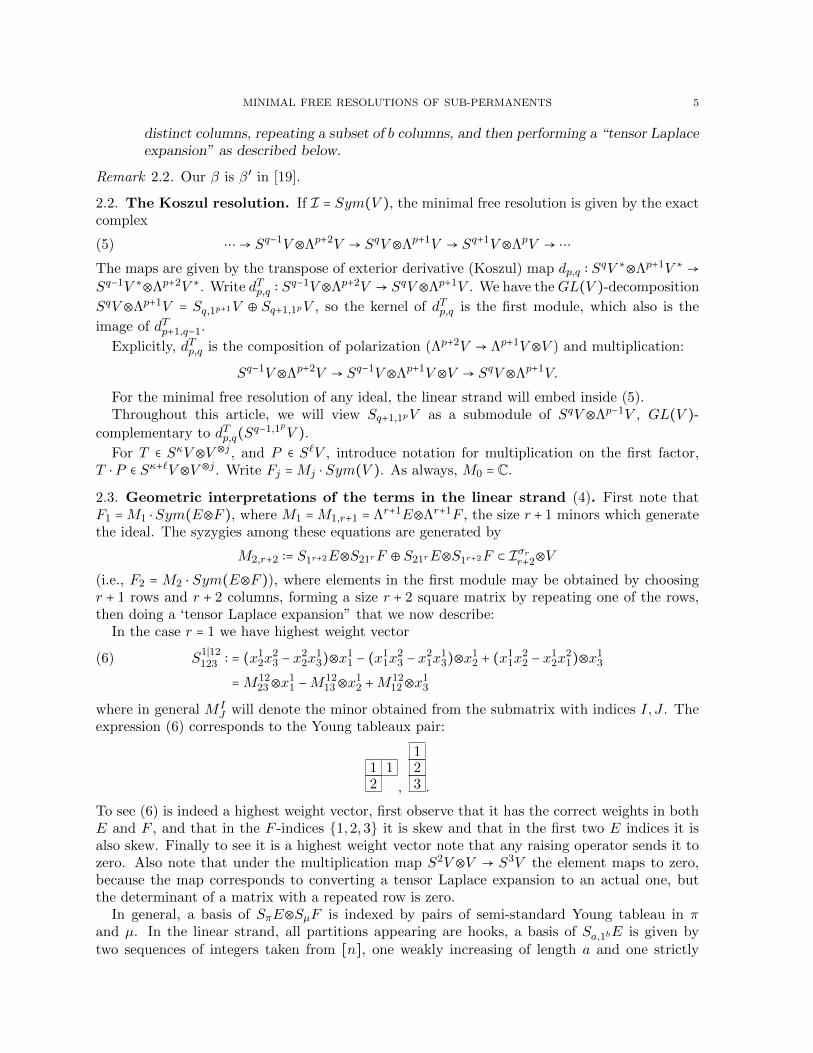
expression (6) corresponds to the Young tableaux pair:

1 12 ,

123 .

To see (6) is indeed a highest weight vector, first observe that it has the correct weights in bothE and F , and that in the F -indices {1,2,3} it is skew and that in the first two E indices it isalso skew. Finally to see it is a highest weight vector note that any raising operator sends it tozero. Also note that under the multiplication map S2V ⊗V → S3V the element maps to zero,because the map corresponds to converting a tensor Laplace expansion to an actual one, butthe determinant of a matrix with a repeated row is zero.

In general, a basis of SπE⊗SµF is indexed by pairs of semi-standard Young tableau in πand µ. In the linear strand, all partitions appearing are hooks, a basis of Sa,1bE is given bytwo sequences of integers taken from [n], one weakly increasing of length a and one strictly


increasing of length b, where the first integer in the first sequence is at least the first integer inthe second sequence.

A highest weight vector in S21rE⊗S1r+2F is

S1∣1,⋯,r+11,⋯,r+2 =M1,⋯,r+1

2,⋯,r+2⊗x11 −M

1,⋯,r+11,3,⋯,r+1⊗x

12 +⋯ + (−1)rM1,⋯,r+1

1,⋯,r+1⊗x1r+2,

and the same argument as above shows it has the desired properties. Other basis vectors areobtained by applying lowering operators to the highest weight vector, so their expressions willbe more complicated.

Remark 2.3. If we chose a size r + 2 submatrix, and perform a tensor Laplace expansion of itsdeterminant about two different rows, the difference of the two expressions corresponds to alinear syzygy, but these are in the span of M2. These expressions are important for comparisonwith the permanent, as they are the only linear syzygies for the ideal generated by the size r+1sub-permanents, where one takes the permanental Laplace expansion.

Continuing, F3 is generated by the module

M3,r+3 = S1r+3E⊗S3,1rF ⊕ S2,1r+1E⊗S2,1r+1F ⊕ S3,1rE⊗S1r+3F ⊂M2⊗V.

These modules admit bases of double tensor Laplace type expansions of a square submatrix ofsize r+3. In the first case, the highest weight vector is obtained from the submatrix whose rowsare the first r+3 rows of the original matrix, and whose columns are the first r-columns with thefirst column repeated three times. For the second module, the highest weight vector is obtainedfrom the submatrix whose rows and columns are the first r + 2 such, with the first row/columnrepeated twice. A highest weight vector for S3,1rE⊗S1r+3F is

S11∣1,⋯,r+11,⋯,r+3 = ∑

1≤β1<β2≤r+3

(−1)β1+β2M1,⋯,r+1

1,⋯,β1,⋯,β2,⋯,r+3⊗(x1

β1 ∧ x1β2)

=r+3

∑β=1

(−1)β+1S1∣1,⋯,ir+11,⋯,β,⋯,r+3

⊗x1β.

Here S1∣1,⋯,ir+11,⋯,β,⋯,r+3

is defined in the same way as the highest weight vector.

A highest weight vector for S2,1r+1E⊗S2,1r+1F is

S1∣1,⋯,r+31∣1,⋯,r+2

=r+3

∑α,β=1

(−1)α+βM1,⋯,α,⋯,r+2

1,⋯,β,⋯,i+2⊗(xα1 ∧ x

1β)

=r+3

∑β=1

(−1)β+1S1,⋯,r+2

1∣1,⋯,β,⋯,r+2⊗x1

β −r+3

∑α=1

(−1)α+1S1∣1,⋯,α,⋯,r+31,⋯,r+2 ⊗xα1 .

Here S1,⋯,r+2

1∣1,⋯,β,⋯,r+2, S

1∣1,⋯,α,⋯,r+31,⋯,r+2 are defined in the same way as the corresponding highest

weight vectors.

Proposition 2.4. The highest weight vector of Sp+1,1r+qE⊗Sq+1,1r+pF ⊂Mp+q+1,r+p+q+1 is

S1p∣1,⋯,r+q+11q ∣1,⋯,r+p+1

=

∑I⊂[r+q+1],∣I∣=q,J⊂[r+p+1],∣J ∣=p

(−1)∣I ∣+∣J ∣M1,⋯,i1,⋯,iq ,⋯,(r+q+1)1,⋯,j1,⋯,jp,⋯,(r+p+1)

⊗(x1j1 ∧⋯ ∧ x1

jp ∧ xi11 ∧⋯ ∧ x

iq1 ).

A hatted index is one that is omitted from the summation.


Proof. It is clear the expression has the correct weight and is a highest weight vector, and thatit lies in Sr+1V ⊗Λp+qV . We now show it maps to zero under the differential.

Under the map dT ∶ Sr+1V ⊗Λp+qV → SrV ⊗Λp+q+1V , the element S1p∣1,⋯,r+q+11q ∣1,⋯,r+p+1

maps to:

∑I⊂[r+q+1],∣I∣=q,J⊂[r+p+1],∣J ∣=p

(−1)∣I ∣+∣J ∣[∑α∈I

(−1)p+αM1,⋯,i1,⋯,iq ,⋯,(r+q+1)1,⋯,j1,⋯,jp,⋯,(r+p+1)

xiα1 ⊗(x1j1 ∧⋯ ∧ x1

jp ∧ xi11 ∧⋯ ∧ xiα1 ∧⋯ ∧ x

iq1 )

+∑β∈J

(−1)βM1,⋯,i1,⋯,iq ,⋯,(r+q+1)1,⋯,j1,⋯,jp,⋯,(r+p+1)

x1jβ⊗(x1

j1 ∧⋯ ∧ x1jβ∧⋯ ∧ x1

jp ∧ xi11 ∧⋯ ∧ x

iq1 )]

Fix I and all indices in J but one, call the resulting index set J ′, and consider the resulting term

∑β∈[r+p+1]/J ′

(−1)f(β,J′)M

1,⋯,i1,⋯,iq ,⋯,(r+q+1)1,⋯,j′1,⋯,j

′

p−1,⋯,(r+p+1)x1β⊗(x1

j′1∧⋯ ∧ x1

j′p−1∧ xi11 ∧⋯ ∧ x

iq1 )

where f(β, J ′) equals the number of j′ ∈ J less than β. This term is the Laplace expansion ofthe determinant of a matrix of size r + 1 which has its first row appearing twice, and is thuszero. �

Notice that if q, p > 0, then S1p∣1,⋯,r+q+11q ∣1,⋯,r+p+1

is the sum of terms including S1p∣1,⋯,r+q1q−1∣1,⋯,r+p+1

⊗xr+q+11

and S1p−1∣1,⋯,r+q+11q ∣1,⋯,r+p ⊗x1

r+p+1. This implies the following corollary:

Corollary 2.5 (Roberts [17]). Each module Sa,1r+bE⊗Sb,1r+aF , where a+b = j that appears withmultiplicity one in Fj,j+r, appears with multiplicity two in Fj−1,j+r if a, b > 0, and multiplicity oneif a or b is zero. The map Fj,j+r+1 → Fj−1,j+r+1 restricted to Sa,1r+bE⊗Sb,1r+aF , maps non-zeroto both (Sa−1,1r+bE⊗Sb,1r+a−1F ) ⋅E⊗F and (Sa,1r+b−1E⊗Sb−1,1r+aF ) ⋅E⊗F .

Proof. The multiplicities and realizations come from applying the Pieri rule. (Note that if a iszero the first module does not exist and if b is zero the second module does not exist.) That themaps to each of these is non-zero follows from the remark above. �

Remark 2.6. In [17] it is proven more generally that all the natural realizations of the irreduciblemodules in Mj have non-zero maps onto every natural realization of the module in Fj−1. More-over, the constants in all the maps are determined explicitly. The description of the maps isdifferent than the one presented here.

2.4. Proof of Theorem 2.1. This section is expository and less elementary than the rest ofthe paper. The variety σr admits a desingularization by the geometric method of [19], namelyconsider the Grassmannian G(r,E∗) and the vector bundle p ∶ S⊗F → G(r,E∗) whose fiber overx ∈ G(r,E∗) is x⊗F . (Although we are breaking symmetry here, it will be restored in the end.)The total space admits the interpretation as the incidence variety

{(x,φ) ∈ G(r,E∗) ×Hom(F,E∗

) ∣ φ(F ) ⊆ x},

and the projection to Hom(F,E∗) = E∗⊗F ∗ has image σr. One also has the exact sequence

0→ S⊗F ∗→ E∗

⊗F ∗→ Q⊗F ∗

→ 0

where E∗⊗F ∗ denotes the trivial bundle with fiber E∗⊗F ∗ and Q = E∗/S is the quotient bundle.As explained in [19], letting q ∶ S⊗F ∗ → E∗⊗F ∗ denote the projection, q is a desingularizationof σr, the higher direct images Riq

∗(OS⊗F ∗) are zero for i > 0, and so by [19, Thm. 5.12,5.13]one concludes Fi =Mi ⋅ Sym(E⊗F ) where

Mi = ⊕j≥0Hj(G(r,E∗

),Λi+j(Q∗⊗F ))

= ⊕j≥0 ⊕∣π∣=i+j Hj(G(r,E∗

), SπQ)⊗Sπ′F


One now uses the Bott-Borel-Weil theorem to compute these cohomology groups. An algorithmfor this is given in [19, Rem. 4.1.5]: If π = (p1,⋯, pq) (where we must have p1 ≤ n to have Sπ′Fnon-zero, and q ≤ n − r as rankQ = n − r), then SπQ

∗ is the vector bundle corresponding to thesequence

(7) (0r, p1,⋯, pn−r).

The dotted Weyl action by σi = (i, i + 1) ∈Sn is

σi ⋅ (α1,⋯, αn) = (α1,⋯, αi−1, αi+1 − 1, αi + 1, αi+2,⋯, αn)

and one applies simple reflections to try to transform α to a partition until one either gets apartition after u simple reflections, in which case Hu is equal to the module associated to thepartition one ends up with and all other cohomology groups are zero, or one ends up on a wallof the Weyl chamber, i.e., at one step one has (β1,⋯, βn) with some βi+1 = βi + 1, in which casethere is no cohomology.

In our case, we need to move p1 over to the first position in order to obtain a partition, whichmeans we need p1 ≥ r + 1, and then if p2 < 2 we are done, otherwise we need to move it etc...The upshot is we can get cohomology only if there is an s such that ps ≥ r + s and ps+1 < s + 1,in which case we get

S(p1−r,⋯,ps−r,sr,ps+1,⋯,pn−r)E⊗Sπ′F

contributing to Hrs. Say we are in this situation, then write (p1 − r − s,⋯, ps − r − s) = α,(ps+1,⋯, pn−r) = β

′, so

(p1 − r,⋯, ps − r, sr, ps+1,⋯, pn−r) = (sr+s) + (α,0r, β′)

and moreover we may write

π′ = (sr+s) + (β,0r, α′)

proving Theorem 2.1. The case s = 1 gives the linear strand of the resolution.

3. The minimal free resolution of the ideal generated by the space of squarefree monomials

The space of (n−κ)-th shifted partial derivatives of the polynomial x1⋯xn ∈ SnCn is spanned

by the set of square free monomials in SκCn (also called the vectors of regular weight, see §4.1).While the ideal these generate has been well-studied, we were unable to find its minimal freeresolution in the literature.

Proposition 3.1. The Hilbert function of Ix1⋯xn,κ in degree κ + t is

(8) dimIx1⋯xn,κκ+t =n−κ∑j=0

(n

κ − j)(κ + t − 1

κ + j − 1)

Proof. The ideal in degree d = t+ κ has a basis of the distinct monomials of degree d containingat least κ distinct indices. When we divide such a basis vector by x1⋯xn the denominator willhave degree at most κ. For each i ≤ κ, the space of possible numerators with a denominator ofdegree i that is fixed, has dimension dimSd−n+iCn−i, and there are (

ni) possible denominators.

Summing over i gives the result. �

For the Hilbert function of the coordinate ring, we have the following expression:

Proposition 3.2. The Hilbert function of Sym(Cn)/Ix1⋯xn,κ in degree t is

(9) dim(Sym(Cn)/Ix1⋯xn,κ)t =n−κ−2

∑j=0

(n

j + 1)(t − 1

j),


if t ≥ n − κ − 1, and (n+t−1n−1

) if t < n − κ − 1.

The expression (9) will be a consequence of the results of the next section.

3.1. The minimal free resolution.

Definition 3.3. [20] A simplicial complex ∆ on a vertex set V is a collection of subsets σ ofV , such that if σ ∈ ∆ and τ ⊂ σ, then τ ∈ ∆. If ∣σ∣ = i + 1 then σ is called an i−face. Let fi(∆)

denote the number of i-faces of ∆, and define dim (∆) = max{i ∣ fi(∆) ≠ 0}. If dim (∆) = n − 1,we define f∆(t) = ∑ni=0 fi−1t

n−i. The ordered list of coefficients of f∆(t) is called the f -vector of∆, and the coefficients of h∆(t) ∶= f∆(t− 1) is called the h-vector of ∆. The Alexander dual ∆∨

of ∆ [16] is the simplicial complex∆∨

= {τ ∣ τ /∈ ∆}

where τ denotes the complement V ∖ τ .

For example, if ∆ is the one skeleton of a three simplex, then f(∆) = (1,4,6) and h(∆) =

(1,2,3), and ∆∨ consists of the four vertices and the empty face.

Definition 3.4. Let ∆ be a simplicial complex on vertices {x1, . . . , xn}. The Stanley-Reisnerideal I∆ is

I∆ = ⟨xi1⋯xij ∣ {xi1 , . . . , xij} is not a face of ∆⟩ ⊆ C[x1, . . . xn],

and the Stanley-Reisner ring is C[x1, . . . xn]/I∆.

The Stanley-Reisner ideal I∆∨ of ∆∨ is obtained by monomializing the primary decompositionof I∆: for each primary component in the primary decomposition (for a square free monomialideal, these are just collections of variables), take the product of the terms in the component.So if

I∆ =⋂j

⟨xij1 , . . . , xijκ ⟩,

then xij1⋯xijκ is a minimal generator of I∆∨ , and all minimal generators arise this way. Ofspecial interest to us is the ideal I∆(n,κ) generated by all square-free monomials of degree κ inn variables; it is the Stanley-Reisner ideal of the κ − 2 skeleton of an n − 1 simplex.

Lemma 3.5. [3, Lem. 2.8] The quotient Sym(V )/I∆(n,κ) is Cohen-Macaulay and has a minimalfree resolution which is linear.

We include a proof along the lines of the above discussion.

Proof. The ideal I∆(n,n−κ) is the Stanley Reisner ideal of the n − κ − 2 skeleton of the n − 1simplex ∆n−1. The primary decomposition of I∆(n,n−κ) is [18, Thm. 5.3.3]

I∆(n,n−κ) = ⋂1≤j1<⋯<jκ+1≤n

(xj1 , . . . , xjκ+1).

Thus, the Alexander dual ideal satisfies

I∆(n,n−κ)∨ = I∆(n,κ).

It follows that the Alexander dual of I∆(n,n−κ) is the Stanley-Reisner ideal of the κ− 2 skeletonof ∆n−1, which is I∆(n,κ). For all κ, the κ-skeleta of the simplex ∆n−1 are shellable [20, p.286],hence I∆(n,κ) is Cohen-Macaulay [16, Thm. 13.45]. The Eagon-Reiner theorem [4] now impliesthat I∆(n,n−κ) has a linear minimal free resolution. Applying Alexander duality shows thatI∆(n,k) also has a linear minimal free resolution and is Cohen-Macaulay. �

If the minimal free resolution of an ideal I has the j-th term Fj , the graded Betti numbersare defined to be bj,u ∶= dimFj,u.


Proposition 3.6. The graded Betti numbers of I∆(n,κ) are, writing Fj,q for the degree q termin the j-th term in the minimal free resolution of I∆(n,κ),

dimFj,j+κ = (n

κ + j)(κ − 1 + j

j),

and the graded Betti numbers are zero in all degrees other than j + κ.

Proof. By Lemma 3.5, the minimal free resolution of Sym(V )/I∆(n,κ) is linear. Hence, therecan be no cancellation in the Hilbert series, and the dimensions of the graded Betti numbersmay be read off from the numerator of the Hilbert series. As the numerator of the Hilbert seriesis the h-vector of the κ − 2 skeleton of ∆n−1 (by [16, Cor 1.15] and remarks following it), theresult follows. �

Example 3.7. Consider the ideal I∆(5,3), consisting of the ten square-free cubic monomials infive variables. The graded Betti numbers bi,j are displayed in a Betti table; starting at position(0,0), the entry (reading right and down) in position (i, j) is bi,i+j . The shift in the secondindex allows the Betti table to reflect the regularity of M , that is, the largest j such the Bettitable is non-zero in row j. The Betti table of the minimal free resolution of I∆(5,3) is

total 10 15 60 – – –1 – – –2 – – –3 10 15 6

So, for example, dimF1,4(I∆(5,3)) = 15.

3.2. The minimal free resolution from a representation-theoretic perspective. First,to fix notation, the ideal is generated in degree κ by xi1⋯xiκ , with I ⊂ [n] and ∣I ∣ = κ. Introduce

the notation Sκ = Sκ ×Sn−κ ⊂ Sn, and if π is a partition of κ, write [π] = [π] × [n − κ] for the

Sκ-module that is [π] as an Sκ-module and trivial as an Sn−κ-module. Recall that for finitegroups H ⊂ G, and an H-module W , IndGHW = C[G]⊗C[H]W is the induced G-module, which inparticular has dimension equal to (dimW )∣G∣/∣H ∣, and that dim[π] is given by the hook-lengthformula. These two facts give the dimensions asserted below.

As an Sn-module the space of generators is

M1 = IndSnSκ

[κ] =min{κ,n−κ}⊕j=0

[n − j, j],

and it has dimension (nκ).

Proposition 3.8. The generator of the j-th term in the minimal free resolution of Ix1⋯xn,κ, asan Sn-module, is

(10) Mj,κ+j−1 = IndSnSκ+j−1

[κ,1j−1],

which has dimension (κ+j−1j

)(nκ+j).

Proof. Let I ⊂ [n] have cardinality κ−1, and let i, j ∈ [n]/I be distinct. Then M2 has generatorsSI,ij ∶= xi1⋯xiκxi⊗xj − xi1⋯xiκxj⊗xi. That these map to zero and are linearly independent isclear, and since they span a space of the correct dimension, these must be the generators of M2.The Sκ+1 action on I ∪ i ∪ j is by [κ,1].


In general, Mj+1 has a basis

SI,u1,⋯,uj =∑α

(−1)α+1xi1⋯xiκxuα⊗xu1 ∧⋯ ∧ xuα ∧⋯ ∧ xuj .

It is clear SI,u1,⋯,uj is a syzygy, and for each fixed I it has the desired Sκ+j-action, and thenumber of such equals the dimension of Mj . �

4. On the minimal free resolution of the ideal generated by sub-permanents

Let E,F = Cn, V = E⊗F , and let Ipermn,κκ ⊂ Sκ(E⊗F ) denote the span of the sub-permanents

of size κ and let Ipermκ ⊂ Sym(E⊗F ) denote the ideal it generates. Note that dimIpermκκ = (nκ)

2.

Fix complete flags 0 ⊂ E1 ⊂ ⋯ ⊂ En = E and 0 ⊂ F1 ⊂ ⋯ ⊂ Fn = F . Write SEj for the copy of Sj

acting on Ej and similarly for F .Write TE ⊂ SL(E) for the maximal torus (diagonal matrices). By [15], the subgroup Gpermn

of GL(E⊗F ) preserving the permanent is [(TE ×SE) × (TF ×SF )] ⋉Z2, divided by the imageof the n-th roots of unity.

As an SEn ×SFn-module the space Ipermn,κκ decomposes as

(11)

IndSEn×SFnSEκ×SFκ

[κ]Eκ⊗[κ]Fκ = ([n]E⊕[n−1,1]E⊕⋯⊕[n−κ,κ]E)⊗([n]F⊕[n−1,1]F⊕⋯⊕[n−κ,κ]F ).

4.1. The linear strand.

Example 4.1. The space of linear syzygies M2,κ+1 ∶= ker(Ipermn,κκ ⊗V → Sκ+1V ) is the SEn ×

SFn-module

M2,κ+1 = IndSEn×SFnSEκ+1×SFκ+1

([κ + 1]Eκ+1⊗[κ,1]Fκ+1 ⊕ [κ,1]Eκ+1⊗[κ + 1]Fκ+1).

This module has dimension 2κ( nκ+1

)2. A spanning set for it may be obtained geometrically as

follows: for each size κ + 1 sub-matrix, perform the permanental “tensor Laplace expansion”along a row or column, then perform a second tensor Laplace expansion about a row or columnand take the difference. An independent set of such for a given size κ + 1 sub-matrix maybe obtained from the expansions along the first row minus the expansion along the j-th forj = 2,⋯, κ + 1, and then from the expansion along the first column minus the expansion alongthe j-th, for j = 2,⋯, κ + 1.

Remark 4.2. Compare this with the space of linear syzygies for the determinant, which has

dimension2κ(n+1)n−κ (

nκ+1

)2. The ratio of their sizes is n+1

n−κ , so, e.g., when κ ∼ n2 , the determinant

has about twice as many linear syzygies, and if κ is close to n, one gets nearly n times as many.

Theorem 4.3. dimMj+1,κ+j = (nκ+j)

2(

2(κ+j−1)j

). As an Sn ×Sn-module,

(12) Mj+1,κ+j = IndSEn×SFnSEκ+j×SFκ+j

( ⊕a+b=j

[κ + b,1a]Eκ+j⊗[κ + a,1b]Fκ+j).

The (nκ+j)

2is just the choice of a size κ + j submatrix, the (

2(κ+j−1)j

) comes from choosing

a set of j elements from the set of rows union columns. Naıvely there are (2(κ+j)j

) choices but

there is redundancy as with the choices in the description of M2.

Proof. The proof proceeds in two steps. We first get “for free” the minimal free resolution ofthe ideal generated by SκE⊗SκF . Write the generating modules of this resolution as Mj . Wethen locate the generators of the linear strand of the minimal free resolution of our ideal, whosegenerators we denote Mj+1,κ+j , inside Mj+1,κ+j and prove the assertion.


To obtain Mj+1, we use the involution ω on the space of symmetric functions (see, e.g. [14,§I.2]) that takes the Schur function sπ to sπ′ . This involution extends to an endofunctor ofGL(V )-modules and hence of GL(E) ×GL(F )-modules, taking SλE⊗SµF to Sλ′E⊗Sµ′F (see[1, §2.4]). This is only true as long as the dimensions of the vector spaces are sufficiently large,so to properly define it one passes to countably infinite dimensional vector spaces.

Applying this functor to the resolution (3), one obtains the resolution of the ideal generatedby SκE⊗SκF ⊂ Sκ(E⊗F ). The GL(E) ×GL(F )-modules generating the linear component ofthe j-th term in this resolution are:

Mj,j+κ−1 = ⊕a+b=j−1

S(a,1κ+b)′E⊗S(b,1κ+a)′F(13)

= ⊕a+b=j−1

S(κ+b+1,1a−1)E⊗S(κ+a+1,1b−1)F.

Moreover, by Corollary 2.5 and functoriality, the map from S(κ+b+1,1a−1)E⊗S(κ+a+1,1b−1)F into

Mj−1,j+κ−1 is non-zero to the copies of S(κ+b+1,1a−1)E⊗S(κ+a+1,1b−1)F in

(Sκ+b,1a−1E⊗Sκ+a+1,1b−2F ) ⋅ (E⊗F ) and (Sκ+b+1,1a−2E⊗Sκ+a,1b−1F ) ⋅ (E⊗F ),

when a, b > 0.Inside SκE⊗SκF is the ideal generated by the sub-permanents (11) which consists of the

weight spaces (p1,⋯, pn)×(q1,⋯, qn), where all pi, qj are either zero or one. (Each sub-permanenthas such a weight, and, given such a weight, there is a unique sub-permanent to which itcorresponds.) Call such a weight space regular. Note that the set of regular vectors in anyE⊗m⊗F⊗m (where m ≤ n to have any) spans a SE ×SF -submodule.

The linear strand of the j-the term in the minimal free resolution of the ideal generated by(11) is thus a SE ×SF -submodule of Mj,j+κ−1. We claim this sub-module is the span of theregular vectors. In other words:

Lemma 4.4. Mj+1,κ+j = (Mj+1,κ+j)reg.

Assuming Lemma 4.4, Theorem 4.3 follows because if π is a partition of κ + j then the weight(1,⋯,1) subspace of SπEκ+j , considered as an SEκ+j -module, is [π] (see, e.g., [7]), and the space

of regular vectors in SπE⊗SµF is IndSE×SFSEκ+j×SFκ+j

[π]E⊗[µ]F . �

Before proving Lemma 4.4 we establish conventions for the inclusions Sq+1,1pE ⊂ Sq+1,1p−1E⊗Eand Sq+1,1pE ⊂ Sq,1pE⊗E.

Let Θ(p, q) ∶ Sq+1,1pE → Sq+1,1p−1E⊗E be the GL(E)-module map defined such that thefollowing diagram commutes:

SqE⊗Λp+1E → Sq+1,1pE↓ ↓ Θ(p, q)

SqE⊗E⊗ΛpE → Sq+1,1p−1E⊗E,

where the left vertical map is the identity tensored with the polarization Λp+1E → ΛpE⊗E.We define two GL(E)-module maps SqE⊗Λp+1E → Sq−1E⊗E⊗Λp+1E: σ1, which is the iden-

tity on the second component and polarization on the first, i.e. SqE → Sq−1E⊗E, and σ2, whichis defined to be the composition of

SqE⊗Λp+1E → (Sq−1E⊗E)⊗(ΛpE⊗E)→ (Sq−1E⊗E)⊗(ΛpE⊗E)→ Sq−1E⊗E⊗Λp+1E

where the first map is two polarizations, the second map swaps the two copies of E and the lastis the identity times skew-symmetrization. Let Σ(p, q) ∶ Sq+1,1pE → Sq+1,1p−1E⊗E denote the


unique (up to scale) GL(E)-module inclusion (unique because Sq+1,1pE has multiplicity one inSq+1,1p−1E⊗E). A short calculation shows that the following diagram is commutative:

SqE⊗Λp+1E → Sq+1,1pEσ2 − pσ1 ↓ ↓ Σ(p, q)

Sq−1E⊗E⊗Λp+1E → Sq,1pE⊗E.

Proof of Lemma 4.4. We work by induction, the case j = 1 was discussed above. Assumethe result has been proven up to Mj,κ+j−1 and consider Mj+1,κ+j . It must be contained inMj,κ+j−1⊗(E⊗F ), so all its weights are either regular, or such that one of the pi’s is 2, and/orone of the qi’s is 2, and all other pu, qu are zero or 1. Call such a weight sub-regular. It remainsto show that no linear syzygy with a sub-regular weight can appear. To do this we show thatno sub-regular weight vector in (Mj,κ+j)subreg maps to zero in (Mj−1,κ+j−1)reg ⋅ (E⊗F ).

First consider the case where both the E and F weights are sub-regular, then (because thespace is a SE ×SF -module), the weight (2,1,⋯,1,0,⋯,0) × (2,1,⋯,1,0,⋯,0) must appear inthe syzygy. But the only way for this to appear is to have a term of the form T ⋅ x1

1, whichcannot map to zero because, since x1

1 is a non-zero-divisor in Sym(V ), our syzygy is a syzygyof degree zero multiplied by x1

1. But by minimality no such syzygy exists.Finally consider the case where there is a vector of weight (2,1j+κ−2) × (1j+κ) appearing.

Consider the set of vectors of this weight as a module for Sj+κ−2 ×Sj+κ. This module is

(14) ⊕a+b=j

[κ + a,1b]/[2]⊗[κ + b,1a].

Here

[κ + a,1b]/[2] = [κ + a − 2,1b]⊕ [κ + a − 1,1b−1]

is called a skew Specht module.By Howe-Young duality and Corollary 2.5 if a, b > 0, Sκ+a,1bE⊗Sκ+b,1aF ⊂Ma+b+1,κ+a+b maps

non-zero to the two distinguished copies of the same module in Ma+b,κ+a+b. This in turn impliesthat the two distinguished copies of Sκ+a,1bE⊗Sκ+b,1aF ⊂ Ma+b,κ+a+b, each map non-zero toMa+b−1,κ+a+b.

The module (14) will take image inside

⊕c+d=j−1

IndSj+κ−1×Sj+κ+1(Sj+κ−2×S1)×(Sj+κ×S1)([κ + c,1

d]/[2]⊗[1])⊗([κ + d,1c]⊗[1]).

Fix a term [κ + b,1a] on the right hand side and examine the map on the left hand side. It is amap

[κ + a,1b]/[2]→ IndSj+κ−1Sj+κ−2×S1

([κ + a,1b−1]/[2]⊗[1])⊕ Ind

Sj+κ−1Sj+κ−2×S1

([κ + a − 1,1b]/[2]⊗[1]).

If b > 0, the map to the first summand is the restriction of the map Θ(b, κ + a) ∶ Sκ+a+1,1bE →Sκ+a+1,1b−1E⊗E, and, due to the fact that it has to map to a sub-regular weight, there is nopolarization because the basis vector e1 has to stay on the left hand side. So the map is theidentity, thus injective.

It remains to show that for b = 0, the map corresponding to the summand b = 0, a = j whichis the restriction of the injective map Σ(0, κ + j − 2) ∶ Sκ+j−1E → Sκ+j−2E⊗E tensored with themap Θ(j−1, κ) injects into the cokernel of the summand corresponding to c = 0, d = j−1 modulothe image of the map coming from the summand a = 1, b = j − 1. Both modules consist of justtwo irreducible SEj+κ−1 ×SFj+κ−1-modules and, using formulas for Σ and Θ, the map is injective.This concludes the proof. �


Example 4.5. For small n and κ, computer computations show no additional first syzygies onthe κ × κ sub-permanents of a generic n × n matrix (besides the linear syzygies) in degree lessthan the Koszul degree 2κ. For example, for κ = 3 and n = 5, there are 100 cubic generatorsfor the ideal and 5200 minimal first syzygies of degree six. There can be at most (

1002) = 4950

Koszul syzygies, so there must be additional non-Koszul first syzygies.

4.2. The Hilbert function in the case κ = 2. First, the Hilbert polynomial:

Theorem 4.6. For the ideal Ipermn,2 of 2 × 2 permanents of an n × n matrix, the Hilbertpolynomial of Sym(V )/Ipermn,2 is

(15)n

∑i=0

fi(t − 1

i),

where fi is the ith entry in the vector

[n2,(n2

2) − (

n

2)

2

,2(n

2)

2

+ 2n(n

3),2n(

n

4),2n(

n

5), . . . ,2n(

n

n)]

Proof. [13, Thm. 3.2] gives a Grobner basis for√Ipermn,2, the radical of Ipermn,2, and by

[13, Thm. 3.3],√Ipermn,2/Ipermn,2 has finite length, so vanishes in high degree. The Hilbert

polynomial only measures dimension asymptotically, so

HP (Sym(V )/√Ipermn,2, t) =HP (Sym(V )/I

permn,2, t).

By [13], for any diagonal term order, the Grobner basis for√Ipermn,2 is given by quadrics of

the formxijxkl + xkjxil with i < k, j < l,

and five sets of cubic monomials

(16)

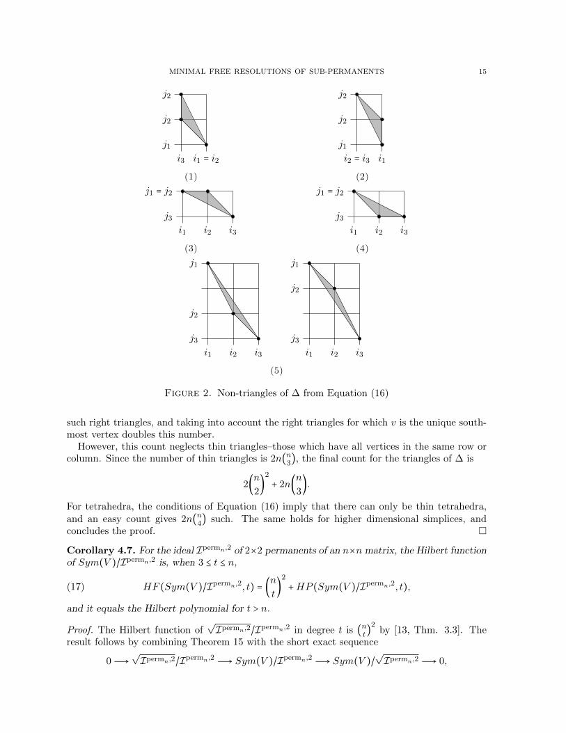
xi1j1xi1j2xi2j3 i1 > i2 j1 < j2 < j3xi1j1xi2j2xi2j3 i1 > i2 j1 < j2 < j3xi1j1xi2j1xi3j2 i1 < i2 < i3 j1 > j2xi1j1xi2j2xi3j2 i1 < i2 < i3 j1 > j2xi1j1xi2j2xi3j3 i1 < i2 < i3 j1 > j2 > j3.

The key observation is that all the cubic monomials are square-free, as are the initial terms of the

quadrics. Thus the initial ideal of√Ipermn,2 is a square-free monomial ideal and corresponds to

the Stanley-Reisner ideal of a simplicial complex ∆. By [18, Lem. 5.2.5], the Hilbert polynomialis as in Equation (15), where fi is the number of i-dimensional faces of ∆. As the vertex set of∆ corresponds to all lattice points (i, j) with 1 ≤ i, j ≤ n, it is immediate that f0 = n

2.Since xijxkl is a non-face if i < k, j < l, no edge connects a southwest lattice point to a

northeast lattice point. Hence, the edges of ∆ consist of all pairs (i, j), (k, l) with i ≥ k and j ≥ l,

of which there are (n2

2) − (

n2)

2.

Next, consider the triangles of ∆. Equation (16) says there are no triangles in ∆ of the typesin Figure 2. Also, there are no triangles which contain an edge connecting vertices at positions(i, j) and (k, l) with i < k,j < l. Thus, the only triangles in ∆ are right triangles, but withhypotenuse sloping from northwest to southeast. For a lattice point v at position (d, e) thereare exactly (d − 1)(e − 1) right triangles having v as their unique north-most vertex. In therightmost column n, there are no such triangles, in the next to last column n − 1 there are(n − 1) + (n − 2) +⋯ = (

n2) such triangles. Continuing this way yields a total count of

(n − 1)(n

2) + (n − 2)(

n

2) +⋯2(

n

2) + (

n

2) = (

n

2)

2


j1

j2

j2

i3 i1 = i2

(1)

j1

j2

j2

i2 = i3 i1

(2)

j3

j1 = j2

i1 i2 i3

(3)

j3

j1 = j2

i1 i2 i3

(4)

j3

j2

j1

i1 i2 i3

j3

j2

j1

i1 i2 i3

(5)

Figure 2. Non-triangles of ∆ from Equation (16)

such right triangles, and taking into account the right triangles for which v is the unique south-most vertex doubles this number.

However, this count neglects thin triangles–those which have all vertices in the same row orcolumn. Since the number of thin triangles is 2n(n3), the final count for the triangles of ∆ is

2(n

2)

2

+ 2n(n

3).

For tetrahedra, the conditions of Equation (16) imply that there can only be thin tetrahedra,and an easy count gives 2n(n4) such. The same holds for higher dimensional simplices, andconcludes the proof. �

Corollary 4.7. For the ideal Ipermn,2 of 2×2 permanents of an n×n matrix, the Hilbert functionof Sym(V )/Ipermn,2 is, when 3 ≤ t ≤ n,

(17) HF (Sym(V )/Ipermn,2, t) = (

n

t)

2

+HP (Sym(V )/Ipermn,2, t),

and it equals the Hilbert polynomial for t > n.

Proof. The Hilbert function of√Ipermn,2/Ipermn,2 in degree t is (

nt)

2by [13, Thm. 3.3]. The

result follows by combining Theorem 15 with the short exact sequence

0Ð→√Ipermn,2/I

permn,2 Ð→ Sym(V )/Ipermn,2 Ð→ Sym(V )/

√Ipermn,2 Ð→ 0,


and additivity of the Hilbert function. �

For the purposes of comparing with other ideals, we rephrase this as:

Theorem 4.8. dimIpermn,22 = (

n2)

2. For 3 ≤ t ≤ n:


t) − [(

n

t)

2

+ n2+ (t − 1)((

n2

2) − (

n

2)

2

) + 2(t − 1

2)((

n

2)

2

+ n(n

3))

+ 2nt−1

∑j=3

(t − 1

j)(

n

j + 1)]

and for t > n:


t) − [n2

+ (t − 1)((n2

2) − (

n

2)

2

) + 2(t − 1

2)((

n

2)

2

+ n(n

3))

+ 2nt−1

∑j=3

(t − 1

j)(

n

j + 1)]

and the latter formula is dimStCn2minus the Hilbert polynomial for all t.

References

1. Kaan Akin and Jerzy Weyman, Primary ideals associated to the linear strands of Lascoux’s resolution andsyzygies of the corresponding irreducible representations of the Lie superalgebra gl(m∣n), J. Algebra 310(2007), no. 2, 461–490. MR 2308168 (2009c:17007)

2. N. Alon and M. Tarsi, A nowhere-zero point in linear mappings, Combinatorica 9 (1989), no. 4, 393–395.MR 1054015 (92a:11147)

3. Riccardo Biagioli, Sara Faridi, and Mercedes Rosas, Resolutions of De Concini-Procesi ideals of hooks, Comm.Algebra 35 (2007), no. 12, 3875–3891. MR 2371263 (2008i:13018)

4. John A. Eagon and Victor Reiner, Resolutions of Stanley-Reisner rings and Alexander duality, J. Pure Appl.Algebra 130 (1998), no. 3, 265–275. MR 1633767 (99h:13017)

5. Klim Efremenko, J.M. Landsberg, Hal Schenck, and Jerzy Weyman, On the method of shifted partial deriva-tives in complexity theory, preprint (2016).

6. William Fulton and Joe Harris, Representation theory, Graduate Texts in Mathematics, vol. 129, Springer-Verlag, New York, 1991, A first course, Readings in Mathematics. MR 1153249 (93a:20069)

7. David A. Gay, Characters of the Weyl group of SU(n) on zero weight spaces and centralizers of permutationrepresentations, Rocky Mountain J. Math. 6 (1976), no. 3, 449–455. MR MR0414794 (54 #2886)

8. Ankit Gupta, Pritish Kamath, Neeraj Kayal, and Ramprasad Saptharishi, Approaching the chasm at depthfour, Proceedings of the Conference on Computational Complexity (CCC) (2013).

9. George A. Kirkup, Minimal primes over permanental ideals, Trans. Amer. Math. Soc. 360 (2008), no. 7,3751–3770. MR 2386244 (2009a:13017)

10. J. M. Landsberg, Geometric complexity theory: an introduction for geometers, Ann. Univ. Ferrara Sez. VIISci. Mat. 61 (2015), no. 1, 65–117. MR 3343444

11. J. M. Landsberg and Giorgio Ottaviani, Equations for secant varieties of Veronese and other varieties, Ann.Mat. Pura Appl. (4) 192 (2013), no. 4, 569–606. MR 3081636

12. Alain Lascoux, Syzygies des varietes determinantales, Adv. in Math. 30 (1978), no. 3, 202–237. MR 520233(80j:14043)

13. Reinhard C. Laubenbacher and Irena Swanson, Permanental ideals, J. Symbolic Comput. 30 (2000), no. 2,195–205. MR 1777172 (2001i:13039)

14. I. G. Macdonald, Symmetric functions and Hall polynomials, second ed., Oxford Mathematical Monographs,The Clarendon Press Oxford University Press, New York, 1995, With contributions by A. Zelevinsky, OxfordScience Publications. MR 1354144 (96h:05207)

15. Marvin Marcus and F. C. May, The permanent function, Canad. J. Math. 14 (1962), 177–189. MR MR0137729(25 #1178)

16. Ezra Miller and Bernd Sturmfels, Combinatorial commutative algebra, Graduate Texts in Mathematics, vol.227, Springer-Verlag, New York, 2005. MR 2110098 (2006d:13001)


17. P. Roberts, A minimal free complex associated to the minors of a matrix, unpublished (1978).18. Hal Schenck, Computational algebraic geometry, London Mathematical Society Student Texts, vol. 58, Cam-

bridge University Press, Cambridge, 2003. MR 2011360 (2004k:13001)19. Jerzy Weyman, Cohomology of vector bundles and syzygies, Cambridge Tracts in Mathematics, vol. 149,

Cambridge University Press, Cambridge, 2003. MR MR1988690 (2004d:13020)20. Gunter M. Ziegler, Lectures on polytopes, Graduate Texts in Mathematics, vol. 152, Springer-Verlag, New

York, 1995. MR 1311028 (96a:52011)

Simons Institute for Theoretical Computing, BerkeleyE-mail address: [email protected]

Department of Mathematics, Texas A&M UniversityE-mail address: [email protected]

Department of Mathematics, University of IllinoisE-mail address: [email protected]

Department of Mathematics, University of ConnecticutE-mail address: [email protected]

introduction - math.tamu.edujml/elswmfr2-29.pdf · key words and phrases. ... perm n∈s n(e⊗f)...

Documents