introduction: an essay on labor cost - core · 3 an essay on labor cost i do not, of course, mean...
TRANSCRIPT

This PDF is a selection from an out-of-print volume from the National Bureauof Economic Research
Volume Title: The Measurement of Labor Cost
Volume Author/Editor: Jack E. Triplett, ed.
Volume Publisher: University of Chicago Press
Volume ISBN: 0-226-81256-1
Volume URL: http://www.nber.org/books/trip83-1
Publication Date: 1983
Chapter Title: Introduction: An Essay on Labor Cost
Chapter Author: Jack E. Triplett
Chapter URL: http://www.nber.org/chapters/c7372
Chapter pages in book: (p. 1 - 60)

1 Introduction: An Essay on Labor Cost Jack E. Triplett
It will require the concentration of the minds of many . . . to make the most basic economic concept and its statistical equivalent fully meaningful for eco- nomic research. Oskar Morgenstern, On the Accuracy of Economic Observations
1.1 Introduction
Prices are at the heart of economic analysis, so much so that the study of the principles governing economic behavior historically has been termed “price theory.” Not surprisingly, economists have expended a great amount of resources on refining concepts that underlie the measure- ment of prices and on evaluating the correspondence of available mea- sures to the conceptual model.’
Wages are no less central to the study of labor markets. And the formal analysis of labor markets used to be called “the theory of wages.” But one looks in vain for labor market literature comparable to that available on the measurement of prices.
One can look at the matter in another way. Traditionally, inputs to the production process have been identified as labor and capital. When volume 45 of this series addressed the measurement of capital (Usher
Jack E. Triplett is associate commissioner, Office of Research and Evaluation, U.S. Bureau of Labor Statistics, Washington, D.C.
The author is indebted to G. Donald Wood, Wesley S. Mellow, B. K. Atrostic, Milton Moss, Daniel S. Hamermesh, and Emst R. Berndt for comments on the draft of this paper; to Richard J. McDonald for helpful discussions on several points; to Julie A. Bunn for research assistance; and to Darlene V. King for efficiently converting the tapes and scribbling she received into a form that can be read by others. Views expressed are those of the author and do not represent official positions of the Bureau of Labor Statistics.
I

2 Jack E. Triplett
1980), it added to an extensive legacy of research that was explicitly concerned with conceptual and empirical measurement problems. It is difficult to cite comparable material on the measurement of labor input and labor cost.
What accounts for this lacuna? Labor economists have often main- tained that wage rates and payment mechanisms are too complex to permit generalization. Orley Ashenfelter noted in the discussion at the Williamsburg conference that a steel industry collective bargaining con- tract contains pages and pages of wage rates for different occupations, grades, skill levels, and so forth. That is, of course, quite true. Yet, Oskar Morgenstern (1963) noted many years ago, in a passage in his classic book on measurement in economics, that the same thing was true of prices in the iron and steel industry. Enormous price heterogeneity exists among different grades and types of steel, different methods of payment, deliv- ery terms, and so forth. (Stigler and Kindahl [1970, p. 51 note some unspecified multiple of 135 million different prices in the price structure for hot rolled carbon steel sheets.) The complexity of the institutional structure of steel pricing has never inhibited economists from generaliz- ing in that area, or from using the basic concepts of economic theory to specify what is wanted of price statistics.
A different set of perceptions may also have suppressed the growth of literature on the measurement of labor market variables. With respect to the measurement of consumption prices and of capital, it has long been recognized that there are formidable and interesting theoretical problems to be attacked. The empirical measurement literature in both of these areas has been stimulated by, and has proceeded in concert with, theoret- ical work (more or less; one could easily cite empirical price measure- ment literature that appears oblivious to, and badly in need of, the theoretical side of the subject). Recognition that labor markets pose equally complex measurement issues has lagged among theorists, and one hears in casual conversation quite the opposite assessment-that labor market analysis contains no particular or unique difficulties. This view, assuming it is widely held, has no doubt inhibited the entry into labor market measurement of the kinds of resources that long have been expended on other areas of measurement in economics. Yet, the theo- rists’ assessment seems highly peculiar: Most of the problems that make capital such a challenging conceptual problem in economics have analogs on the labor side. And in a number of respects, labor markets pose more complex and interesting theoretical problems than the ones usually con- sidered in the measurement of, say, consumer prices.
I will elaborate on these matters later in this essay. It is sufficient to note here that neither the labor economists’ idea that the subject is too complex nor the theorists’ notion that it is too simple justifies the neglect of labor market measurement issues.
3 An Essay on Labor Cost
I do not, of course, mean to suggest that the contributions of theorists and labor economists are without value in understanding the measure- ment of wages, compensation, or labor cost. Clearly, much of the work on price indexes is transferable to labor market measurement. And the literature on capital, having (as is must) analogs on the labor side, suggests approaches that are fruitful.
It is also quite true that a vast amount of recent quantitative research by labor economists, and a fair amount of the work of the older institutional- ist school as well, does have implications for the kinds of data that are relevant and necessary for economic analysis of labor markets. Research on “earnings functions” clarifies earnings concepts (see Griliches 1977), as does exploration of “compensating differentials” (C. Brown 1980); work on the relation between education and productivity defines the units in which labor input is appropriately measured.
Much of the measurement work in labor economics, however, has reflected a labor supply perspective. When innovations in theoretical labor market measurement concepts have occurred, they have had sup- ply-side orientations: The work of Pencavel (1977) and Cleeton (1982) concerns the concept of real wages-that is, worker income. Most new data sets developed over the last two decades represent responses to the perceived need for data to study worker behavior. (I have in mind not only the establishment of the National Longitudinal Surveys of Labor Market Experience, the Panel Study of Income Dynamics, and the several Income Maintenance Experiments, but also the relatively recent exploitation of the panel properties in the Current Population Survey to produce analytic data which can be used to examine worker behavior.)2
Though research can often be milked for implications for economic behavior on both sides of the market, there is a dearth of direct explora- tion of employers’ behavior toward their work forces, and very little data exist for addressing such questions. The demand side of the labor market has been neglected in research, in conceptual work, and in data de- velopment . 3
To claim that existing research lacks implications for measurement in labor markets would be extravagant and untrue. I do maintain that the effort expended on drawing implications for economic measurement from existing knowledge about the operation of labor markets has been sparse relative to other areas of economics, and the balance of that effort has been disproportionately on the supply side.
Thus, not only to hold the subject matter within reasonable bounds, but also to push the measurement literature in the direction of the greatest gaps, the program of this conference was organized to focus on labor cost, rather than on “compensation” or “earnings” as a measure of worker income. Obviously, this distinction is somewhat artificial and is neither strictly nor uniformly maintained in the papers included in this
4 Jack E. Triplett
volume. The labor cost focus does, however, define the perimeters of this introductory essay, which has been conceived as an introduction to the subject of the conference, not as a summary of its individual contribu- tions.
This essay has one main and one subsidiary theme. The principal theme concerns the conceptual framework for measuring the cost of employing labor-the measurement of a factor price. Its initial statement in section 1.2 is abstract and simplified, based on a highly stylized model of production cost; it is developed and expanded in subsequent sections to accommodate relevant empirical knowledge of labor markets. The perspective on this research is intended to highlight the distinction in economic measurement between demand-side and supply-side measure- ment concepts. The subsidiary theme draws parallels and contrasts for labor cost measurement from the theoretical and empirical price mea- surement literature.
1.2 The Theoretical Concept of Labor Cost
By the term “labor cost” I mean the employer’s cost of hiring an incremental unit of labor. The labor cost concept concerns the definition of a factor price: It is the cost of a unit of input (and not a measure of the cost of the labor content of a unit of output). I use “labor cost,” rather than “factor price” or “wage,” to acknowledge the complexity of labor hiring costs and to emphasize that all costs of employment are included, not just direct wage payments. And I use “labor cost” in preference to “compensation” because the latter connotes a measure of labor income, which differs conceptually and empirically from a measure of factor cost.
Labor cost measures are wanted for diverse purposes, for example, production function estimation, inflation analysis, and forming intertem- poral, interarea, or interindustry judgments about the cost levels or cost experiences of different classes of employers. The most flexible data for analytical purposes are microdata-labor cost levels (i.e., dollars per period) for individual employers, with abundant detail on cost compo- nents, plus labor force and employer characteristics. For aggregated or tabulated data, analytical needs specify that published data be available at detailed occupational, industrial, and regional disaggregations, again with detail on components of labor cost.
However the data are presented, some aggregation is normally re- quired to conserve resources-either the user’s or those of the compiling statistical agency. Microdata on firms (such as the data employed by Smith and Ehrenberg in this volume) are normally aggregated over workers. Moreover, under the hedonic view of labor markets even the wage rate or labor cost measure for a single worker is an aggregation of lower order cost measures when labor is not homogeneous, as shown in
5 An Essay on Labor Cost
section 1.6. To begin with the theory of aggregate measurements is not idle theorizing, but is rather a statement of the necessary starting place for any systematic exploration of measurement issue^.^
For a measure of input cost, aggregation rules can be extracted from the economic theory of production and of production cost. Aspects of the theory are discussed in the Gollop-Jorgenson and McMenamin-Russell papers in this volume (see also Diewert 1980, and Caves, Christensen, and Diewert 1982). For present purposes, production theory is highly stylized. Yet, most of the empirical and conceptual issues discussed in this volume can be interpreted as attempts to extend and to make more realistic the stylized picture of the labor market depicted in the theory of demand for inputs.
(1) Q = Q ( K , L , MI,
where Q is output, K and L are vectors of the various types of capital and labor services employed, and M is a vector of materials usage. The elements of the L vector may be thought of as different occupations, different skill groupings or human capital levels, and so forth. It is assumed that each element of the L vector groups workers who are homogeneous. A similar interpretation holds for the K and M vectors.
Beginning the analysis with a production function implies that it applies to an establishment or plant, or to a production process within an estab- lishment. Because “industry” can be defined as a group of establishments having closely related production processes, input cost measures can be rationalized for an industry or for industry groups by appeal to the Marshallian notion of the “representative firm,” though that rationaliza- tion may need elaboration to incorporate heterogeneity in firm size and entrepreneurial inputs, as emphasized by Oi in the present volume. Despite the continued popularity of aggregate, nationwide production functions in a variety of empirical applications, we take it as evident that none exists. Economy-wide measures of factor costs are best interpreted as averages of individual industry measures (the same interpretation applies to aggregate productivity measures or to any other measurement that is derived from a production theoretic point of view).
Associated with equation (1) is a production cost function, which shows total production cost as a function of input prices, given that input quantities are combined in such a way as to minimize production cost for each output level. To keep notation compact, this cost function is de- noted by
(2) C = C ( R , W , P; Q ) , where R, W, and Pare understood as vectors of the costs per unit of input for the various productive factors contained in the vectors K, L, and M ,
We begin from a production function

6 Jack E. Triplett
respectively. For a casual labor market, the cost of a unit of labor is primarily the wage rate. Similar simplifications are usually made with respect to unit capital service costs (rental rates) and materials prices.
When the level of output is fixed, the cost function of equation (2) gives the minimum cost necessary to reach a particular production isoquant . Further, when relative prices vary, with output held constant, the cost function will yield different cost levels corresponding to varying points on the isoquant. Such points-minimum cost combinations of factor inputs that lie on the same production isoquant-provide a natural basis for comparisons of aggregate input price levels. A ratio of these points is called an index number-in this particular case, an “input cost index. ” 5
An index number is thus an aggregation that is grounded on an eco- nomic concept. It can be used for making statements about interarea or interfirm differences of levels, as well as for the more familiar intertem- poral computations.
Most of the content of the economic theory of index number measure- ments (see Samuelson and Swamy 1974, or Diewert 1981) concerns the following three topics.
The Form of the Index Number
An index number computation that is consistent with a specified pro- duction or cost function is termed an “exact” index for the underlying cost or production function (Diewert 1976). The form or “formula” of an exact index number depends on the mathematical form of the cost function (which, in turn, is derived from the form of the production function). Gollop and Jorgenson, for example, present index numbers that are exact for a translog production function.6
Goodness of Approximations
Widely known standard index number formulas, such as Laspeyres or Paasche or Fisher’s Ideal, use only price and quantity information, not the full cost function, They can be interpreted as approximations to the theoretically correct, or exact, index numbers. They are approximations because their input quantity weights can only approximately hold output constant over the index comparison. The exact index number, because it is formed from two points on the same production isoquant, holds output exactly constant. With the approximations, an output error of undeter- mined size is introduced into the index every time the fixed input assump- tion is violated by changes in relative input prices (the well-known “substitution bias” of fixed-weight indexes). Recent empirical and theoretical work indicates that good approximations to exact indexes can be computed from fixed-weight or related formulas.’
Ordinary regressions that include a dummy variable for time, region, or some other variable of interest can also be interpreted as approxima- tions to exact index numbers. The properties of the approximation are
7 An Essay on Labor Cost
usually unclear unless the relation between the regression and the cost function is known.
Subindexes
One frequently wants a measure less aggregative than the index of all input costs. An index of labor cost is one of these “midlevel” aggrega- tions-a measure of the aggregate employment cost of all occupations or labor groups in the W vector of equation (2). Following Pollak (19754, the labor cost index is termed a “subindex” of the full input cost index. The Bureau of Labor Statistics (BLS) “Employment Cost Index” (de- scribed in Antos, this volume) is such a subindex. Lower level subin- dexes, such as a labor cost index for blue-collar workers, may also be desired.
Three results from the theory of subindexes are important for the present discussion. First, though it is natural to suppose that an index of labor cost would require only data on labor, this is true only for special cases. As McMenamin and Russell note in their paper in this volume, Blackorby, Primont, and Russell (1978) have shown that only when the cost function is separable on its labor component will the labor cost subindex be independent of capital service costs, materials prices, and technology. This separability condition is roughlys equivalent to saying that optimal combinations of engineers and laborers do not depend on the proportions of machines and shovels used in the production process, or on the technology and mix of energy and other materials employed- clearly a condition unlikely to be satisfied empirically. Pollak (1975~) considers the interpretation of subindexes when the separability condi- tions do not hold.
Second, the aggregate input cost index will not necessarily be con- structed out of subindexes for capital, labor, and materials costs (R, W , and P). In other words, subindexes constructed in the theoretically appropriate way do not necessarily “add up” in the manner of ordinary fixed-weight index number formulas.
Third, if the theoretical conditions for the aggregation of labor inputs hold empirically (or if they are just maintained), the exact subindex of labor cost can be approximated by a conventional index number formula, such as Laspeyres or Paasche, in a way analogous to the case of the full input cost index.
One would like the theory to provide the conceptual underpinnings for aggregate measures of labor cost. Beyond this, the underlying conceptual framework used in the measurement design provides internal consistency in the data and determines its relevance for the intended use; for this reason, even if researchers use micro data, rather than some aggregate index number, the conceptual measurement model is an issue for all data employed for research.
Use of the standard theory of production to guide labor market
8 Jack E. Triplett
measurement implies difficulties in two areas-restrictiveness, and real- ism or relevance. With respect to the restrictiveness problem, production aggregation theory tells us that stringent separability conditions must be met for labor input or labor cost to be a valid aggregation, and knowledge of production suggests that these conditions are unlikely to hold. For example, Berndt and Christensen (1973) rejected the proposition that white-collar and blue-collar labor could be aggregated, no doubt partly because white-collar labor and capital structures were found to be com- plements. Grant and Hamermesh (1981) examined five labor categories and (aggregate) capital, and likewise found no support for labor aggregation .9
Moreover, whatever may be true for capital and labor inputs, the line separating capital and labor costs frequently becomes blurred, particu- larly for costs of safety, workplace amenities, and other aspects of em- ployment that contribute to what labor economists call “compensating wage differentials.” For these cases, employers (or some third party) can influence labor cost (a price) by use of a larger quantity of capital or some other input.
Even though separability is a required condition for the construction of consistent labor cost measures, the consequences of violation of the separability conditions are empirical, and in some cases may not be all that serious. Berndt and Christensen (1974) find that assuming labor separability when it is untrue has little consequence for using factor quantities to analyze output and productivity movements, but seriously distorts the prediction of factor shares; since the latter use would employ factor prices as data, their finding reinforces our concern.
In any event, there is little in the theory or the empirical knowledge of production that validates the normal disposition of economists to think of “labor” and “capital” as natural aggregations. The conventional practice has mainly custom and supply-side considerations behind it.
With respect to the relevance of the model, it should be emphasized that the stylized production cost model, or close alternatives, is in com- mon use in empirical research. It hardly represents a methodological straw man. The degree of realism in the model underlying empirical research is a compromise that depends on the problem at hand. Yet, it is beyond debate that the stylized model needs more descriptive realism to engage many of the empirical issues of the day.
There are at least four major respects in which the stylized model of production cost is inadequate. Though the Williamsburg conference did not give full attention to all four, it will nevertheless be convenient to discuss relevant research in labor markets and its implications for the measurement of labor cost in terms of these four topic areas.
1. In the stylized model, it is assumed that only wages matter as a measure of factor cost. That assumption need not necessarily be iden-

9 An Essay on Labor Cost
tified with a view that benefits and job amenity costs do not exist or that they are small enough so that their level can be ignored (a view that would probably be ascribed to by almost no user of the stylized model). Rather, it says (a) that total compensation is a simple addition of the cost of benefits to the cost of direct wage payments, and (b) that benefit levels are so strongly correlated with wages that little additional information on labor cost is imparted by gathering data on benefits. I believe this point of view is quite widespread, as it implicitly underlies a great amount of research on labor markets. These issues are addressed in section 1.3 of this essay.
2. The stylized model ignores time dimensions in employment ar- rangements, as well as time dimensions inherent in payment mechanisms. In effect, the stylized model depicts a casual labor market in which neither workers nor employers have any interest in each other after the completion of, and payment for, the current period’s labor services. Of course, both employers and workers do care about the stream over time of labor services provided and payments received, a fact that has moti- vated much recent labor market research. The implications for measuring labor cost are discussed in sections 1.4 and 1.5.
3. The stylized model implies that there is some level of aggregation of the labor input below which one can view workers as homogeneous. The model is inchoate on problems of labor quality that cannot be handled adequately by grouping. Methods for allowing for labor quality in a labor cost measure are discussed in section 1.6.
4. Partly because it relates to a single employer’s decision making, the stylized model is silent on the heterogeneity of employers and of employ- ment conditions. However, just as employers care about the productive characteristics of workers, workers care about the characteristics of em- ployers. This is a major contrast with the framework usually employed for the analysis of product markets, in which one usually assumes that the seller exchanges a package of commodities (this is the hedonic view of markets) for a money payment, but does not demand a package of commodities in return. Labor market transactions, however, involve exchanges of packages on both sides of the market. This assures addi- tional complexity that is ignored in the stylized model. This topic is addressed in section 1.6. The empirical importance of the heterogeneity of employers is also a major theme of Oi in this volume, and that discussion need not be duplicated here.
1.3 Benefits
Recognition of the importance of employer provided benefits in calcu- lating labor cost goes back many years. Legally mandated benefit costs (principally social security and unemployment compensation) first
10 Jack E. Triplett
assumed importance in the 1930s. Negotiated benefits grew faster than wages during World War I1 because those costs were less tightly con- trolled than were direct wage payments. (McMenamin and Russell in this volume indicate the same thing was true of “controls” programs in the 1970s.) Both classes of benefits have grown steadily over the intervening years, whether measured in absolute terms or as a percentage of labor cost, a fact well known and tabulated in the Smeeding and Hamermesh papers in this volume.
Employer provided benefits pose a number of issues for the measure- ment of labor cost. The wage-benefit model sketched in section 1.3.1 serves to organize the discussion of empirical issues in the following sections.
1.3.1 A Wage-Benefit Model
A crucial parameter in analyzing the size and composition of employer provided benefits is the wage that “workers would forgo to obtain the benefit” (Freeman 1981, p. 491). We assume that workers gain utility from benefits (B) , from the goods and services they purchase with direct wage payments (G), and from leisure (T,, - L). The worker’s full income constraint is
(3) To(W + JIBIL) = JIB + PG + (W + JIBIL) (To - L ) ,
where To is total time available, W the hourly wage, BIL the hourly benefit earning rate, P and G the price and quantity of consumption goods, L hours worked, and JI the shadow price of benefits.’” Assuming benefits earned per hour are independent of hours worked, when an hour of leisure is consumed a worker gives up the quantity of goods that an hour’s labor earns (WIP) and an hour’s worth of benefits, BIL. Accord- ingly, we may write the labor supply of workers of a specified quality to the firm” as:
(4) L = L( WIP, BIL) .
Setting P equal to unity, one can invert the labor supply condition, giving
( 5 ) W = W(B , L , 1).
Equation ( 5 ) states that the wage that must be paid by the employer depends on the number of hours of worker input hired and on the level of benefits.
The theory specifies that
(6a) a WIaB 5 0 ;
(6b) awiaLro;
That workers will accept lower wages for greater benefits, or demand higher wages if benefits are lower (condition [6a]), is a consequence of

11 An Essay on Labor Cost
assuming that market purchased goods and services and employer pro- vided benefits are both normal goods, though the lower limit of the workers’ willingness to substitute is zero. For the conventional competi- tive firm, the change in wages necessary to expand or contract the firm’s labor force while minimizing cost (condition [6b]) is zero; for other cases, the normal presumption is that higher wages must be paid to attract more workers, so condition (6b) will be positive. The analysis at this point abstracts from dynamic considerations, so that the rate of hiring does not enter into equation ( 5 ) , only the level of employment (see Phelps et al. 1970).
Though there may be scale economies to the provision of benefits (it may be cheaper per worker for the employer to buy a group insurance policy than for each worker to obtain the same coverage in an individual policy), it seems reasonable to assume that the marginal cost of increasing the size of a benefit is positive and either constant (for example, the cost of $Wl i f e insurance is Utimes the cost of an $Vpolicy) or rising. Thus, if Ei is the employer’s expenditure on benefit Bi,
(7)
The firm will arrange its package of wages and benefits to minimize the cost of hiring L workers, given the above conditions. The cost-minimizing conditions determining the optimal amounts of benefits to be provided are
(8) dEiIdBi = -aW1dBi, for all i .
Equation (8) says that employers offer benefits up to the point where the incremental cost of each benefit just equals the saving in wage cost that can be gained as a result of offering the benefit.’* The wage rate offered is determined by simultaneously solving equation (5) for the desired level of L.
An implication that will be useful later is that a benefit will be increased only when the quantity on the right-hand side of equation (8) is greater (in absolute value) than that on the left-hand side. Since the left-hand side is always positive, this implies that employers will not offer a benefit unless the workers’ wage-benefit trade-off for that benefit is greater than zero. We return to this point in section 1.3.3.
A number of factors may be expected to influence the parameters of this model:
1. Assuming benefits are normal goods, more will be demanded at higher income levels. This will increase the value of B in equation (4) for any given L , regardless of the effect on condition (6a). Moreover, the absolute value of (6a) may itself grow larger with income if benefits are more income-elastic than market purchased goods, thus strengthening the positive relation between benefits and wage rates.
12 Jack E. Triplett
2. When benefits are not taxed, but wage payments are, this increases the wages that workers would forgo to get benefits. From the workers’ point of view, what is being surrendered is not consumption goods with a value equivalent to aEi/aBi (the employers’ marginal cost of providing the benefit), but rather goods having the value of (dEi/aBi).(l - t), where t is the marginal tax rate.I3 Thus, higher marginal tax rates will increase the absolute value of (6a), when that condition is computed on before-tax wage data.I4
3. Empirically it has been shown (Freeman 1981 and Mellow 1982) that unions increase the share of benefits in total compensation, presum- ably by increasing the absolute value of (6a). The precise mechanism for this union effect is un~1ear.l~ 4. Speculation has it that demographic factors may also affect the
value of (6a), with older workers, for example, possibly having greater preferences for benefits than younger ones, and married workers greater than single ones. Women may have different preferences for benefits than do men, but the effect on (6a) could go either way. The “working spouse” model would lower values for (6a), on the grounds that a spouse participates in health plans and so forth provided by the spouse’s em- ployer (this argument applies as well to married men, as the family’s need for health care would be met by whichever worker received the most favorable terms from his or her employer); on the other hand, the “single parent” model of female preferences should produce higher values for (6a), and hence, in this case, women would demand greater levels of benefits, other things equa1.16
The preceding four factors originate from the workers side. The level of benefits is also responsive to factors that affect the employers’ cost of providing benefits.
5. Mellow (1982) and Oi (this volume) present evidence that large firms supply more benefits, partly because their size gives them scale economies in purchasing them. Mitchell and Andrews (1981) present evidence supporting the existence of scale economies in pension plan administration. In the case of scale economies, the level of benefits goes up because the left-hand side of equation (8) falls. Oi, in this volume, suggests other reasons for an association between firm size and benefit levels.
6. Many benefits (pensions and vacations, for example) are inter- locked with tenure and therefore with firm-specific human capital. This says that equation (@-which predicts that wages and benefit costs trade off at equilibrium on a dollar-for-dollar basis-needs to be modified to accommodate cases where there are other important labor cost compo- nents (hiring and turnover costs, for example) that are impacted dif- ferently by wage and benefit changes.
7. Condition (8) also needs modification where workers and em- ployers have time horizons for the employment decision such that estima-

13 An Essay on Labor Cost
tion of a single period’s labor cost (or worker compensation) must accommodate to a multiperiod optimization plan (these considerations motivate the “implicit contract” literature). The last two extensions of the wage-benefit model are left for section 1.4.
1.3.2 Do Benefits Matter?
For computing trends in labor cost, it is clear that benefits must be included. Were benefits omitted, time series analyses would understate the growth in labor cost.
But for other analytical purposes, labor economists disagree whether the omission of benefits from labor cost measures is necessarily a serious liability. A widely used undergraduate textbook (Fleisher and Kniesner 1980, p. 23) states one position on this issue:
When measures of the cost of fringe benefits are not available, the question arises, To what extent is the analysis of labor markets affected? . . . [I]n general it is probably true that the amount of fringe benefits is positively related to nominal wage rates. Thus, the principal effect would be to understate real wage costs more or less consistently by a fraction. The effect of this error on most studies is probably relatively unimportant.
In the following, we refer to this point of view as the “consistency” hypothesis.
The consistency hypothesis is not necessarily at odds with the theoreti- cal model of section 1.3.1. Solutions to the labor cost minimization problem could “stack up” along a path of constant benefit-to-wage proportions, so that wage rates would be a consistent fraction of labor cost for all employers and all groups of workers. For the consistency hypothesis to hold in data for workers at the same earnings level, those workers must all have similar utility functions, and employers must incur similar costs for providing benefits. For consistency to hold across earn- ings levels, in the absence of taxes, unitary income elasticities, both for market-purchased goods and for benefits, are required, plus constant marginal cost schedules for benefits. When taxes enter the system, and wages but not benefits are taxed, marginal rax rates must vary with (nonunitary) income elasticities so that the effects just offset each other, or so that the combined effect just balances any change in the employer’s marginal cost of providing benefits. Whether the consistency hypothesis is true is therefore an empirical matter, which requires a fortuitous confluence of values of the economic parameters that determine the proportion of benefits in total labor cost.
Several papers in the present volume provide evidence on the con- sistency hypothesis. Both Smeeding and Leibowitz ask whether the addi- tion of benefit costs (and in Smeeding’s case the value of benefits to recipients) to ordinary wage measures changes the results of standard

14 Jack E. Triplett
human capital earnings equations. Both authors conclude that one gets the same results from earnings equations that contain only wages as from those where the dependent variable is augmented to include benefit costs.
Neither conclusion, however, is unchallenged. Smeeding himself notes that the microsimulation methods he uses to construct his data base have a tendency to reduce the variance of the benefits data, a point emphasized and elaborated upon by Martin David in his comment. In effect, micro- simulation methods have imposed or partly imposed the consistency hypothesis on the data, so it is not too surprising that the empirical results support the hypothesis.
Leibowitz’s data are from a new and relatively unexplored survey and would appear to be ideal for testing the consistency hypothesis. However, Atrostic points out in her comment that Leibowitz’s benefits data cover only roughly a third of total benefit costs as measured in other surveys, and she presents evidence that the consistency hypothesis holds only for those benefits that were included in Leibowitz’s survey; the hypothesis is rejected when other benefits (especially pension cost) are added to the list.
In summary, then, we have two authors who present results supporting the consistency hypothesis, but those commenting on their papers (and one of the authors himself) emphasize deficiencies in the data employed for their tests.
Complete agreement will never be found between any two sets of data, so determining whether the addition of benefits to wages matters at all is not a very interesting question. The relevant issue is: How much does it matter? How does one determine whether an alternative concept of labor cost (for example, one inclusive of benefit costs) is really “better”?
Hamermesh deals with the issue in a way that stresses its economic relevance. He asks whether the measurement change affects an economi- cally relevant result (labor demand elasticities),” and whether the change in measurement concept moves the estimate in the direction that would be predicted from econometric theory.
He finds that the addition of benefit costs and other aspects of labor cost to the normal average hourly earnings measures increases the esti- mated elasticity of demand for labor, and he argues that this result is predicted on a priori grounds. That is, if labor cost were mismeasured, an errors-in-variables econometric argument suggests that labor demand elasticity estimates are biased toward zero. Thus, the fact that elasticity estimates increase when benefits are added to wages indicates that the labor cost measure inclusive of benefits is the better one, even though the change in the elasticity estimates is not statistically significant. Lazear is not fully convinced by this argument, emphasizing instead that what appear to be the theoretically preferable labor cost measures do not always perform “best” (though it is not addition of benefits to hourly

15 An Essay on Labor Cost
wages that Lazear most questions but some of the other Hamermesh adjustments).
Freeman’s (1981) orientation is similar to that of Hamermesh, for he indirectly tests the consistency hypothesis by comparing alternative esti- mates of the economic effect of unions. The union effect on compensa- tion (wages plus benefit costs) is roughly 17 percent, compared with a 15 percent union differential measured from wages alone. l8 From this and other results, Freeman concludes that “standard estimates of the union wage effect understate the differential between unionized and otherwise comparable nonunion workers” (Freeman 1981, p. 509). Other research on the consistency question has been done by Duncan (1976), Atrostic (1981), and Mellow (1982).
It seems doubtful that consistency between wage and benefit costs will be great enough to warrant the omission of benefits from labor cost data. The relatively recent expansion of the BLS Employment Cost Index to include benefits seems a justified and necessary improvement that makes it a better measure for analytic purposes.
1.3.3 Is There a Market Trade-off between Wages and Benefits?
This is an old research chestnut. Few issues in labor economics have provoked more controversy than this one. The controversy reflects the persistence of the theoretic-institutionalist split in this field (see the exchange between Dunlop 1977 and Ehrenberg, Hamermesh, and John- son 1977).
On the one hand is the theoretical position. If employers are cost minimizers and workers are utility maximizers, then it must be true that, other things equal, a market trade-off between wages and benefits exists.
The labor market institutionalists’ response says, more or less, that the theory may predict a negative trade-off, but the labor market does not work that way. The institutionalist school frequently cites evidence that wages and benefits are positively correlated-the highest paying jobs have the highest benefits. This, of course, is predicted by the theory itself, as noted in section 1.3.1. The theory does not state that the president of the company should receive lower benefits than the janitor, but rather that the negative trade-off between wages and benefits will be found at comparable skill levels and at comparable levels of total compensation. The negative trade-off occurs for job comparisons for which other things are held equal.
Smith and Ehrenberg in the present volume attempt to assemble a body of data in which other things can be held constant in order to test the theoretical prediction of a negative trade-off between wages and benefits. Their study fails to produce evidence to confirm the negative trade-off hypothesis, though the authors argue that a more elaborate data set is

16 Jack E. Triplett
required to perform an adequate test; their conclusion is endorsed and enlarged upon by Charles Brown in his comment.
It is surprising that the wage-benefit trade-off question should have become a serious research issue. It was pointed out in section 1.3.1 that the theoretical model implies that wherever the wage-benefit trade-off does not exist, employers will offer no benefits (see eq. [8]). Thus, testing for the existence of a negative wage-benefit trade-off can be pursued with a much simpler research strategy than the one followed by Smith and Ehrenberg. All one has to do to “test” for the existence of a wage-benefit trade-off is to find out whether employer provided benefits exist!
Of course, such a test will hardly satisfy the critics of a theoretical approach to labor market analysis, for taking an empirical prediction as an implication-and therefore a test-of the theory requires accepting the relevance of the theory, and that is exactly what the critics deny. They argue that firms are not cost minimizers, that workers are not utility maximizers, or that the labor market contains so many deviations from market equilibrium that the exceptions overpower the generalizations. If the critic does not accept the relevance of the theoretical model for labor market research, it is very unlikely that testing the wage-benefit relation for a negative slope will do much to settle the issue, or that any research results based on implications of a theoretical model will convince.
Serious research on relations between wages and benefits has to take the existence of a wage-benefit trade-off as a necessarily true axiom. And if one accepts the theoretical model, it is unnecessary to design a compli- cated research project to confirm it, for the most elemental fact of the labor market (that benefits do exist) provides sufficient evidence that the wage-benefit trade-off part of the theory is true.
It is quite a different story if one wishes to estimate the size of the wage-benefit trade-off. That is a reasonable research project. However, research on the slope of the wage-benefit trade-off function must consider labor cost components other than wages or benefits. This is easily shown.
Suppose the firm’s labor cost is composed of three groups of cost components-direct wage and salary payments ( W ) , benefits expressed as quantities ( B ) , and the hiring and turnover rate (H). Labor cost per unit of labor is
(9) LC = W + OLB + y H ,
where OL is the cost per unit of benefits ( = aEilaBi in eq. [7]), and y is the cost of a unit change in the turnover rate. Assuming no scale economies in the provision of benefits and constant cost for each hirehumover, the usual mathematical manipulation gives expressions for the wage-benefit trade-off , which are:
(10a) - aWlaB = OL + y(aH1aB) ,

17 An Essay on Labor Cost
or
dW/d(aB) = 1 + ( y h ) (dHIdB).
Thus, from the employer’s point of view, minimization of the labor cost function implies that the (negative) trade-off between the quantity of benefits and wages equals the marginal cost of benefits (as in eq. [8]) plus the cost of any change in turnover induced by changing the level of benefits. Alternatively (eq. [lob]), benefit costs and wage costs trade off on a one-for-one basis in the employer’s labor cost function only when benefits have no effect on turnover (aH/dB = 0), or when turnover has no
Neither of the latter two conditions is at all probable. In fact, benefits that are related to tenure-vacations and pensions, for example-are frequently designed to reduce turnover (further implications of turnover costs are discussed in section 1.4). In the presence of turnover costs, reducing benefits by (say) one dollar and raising wages by one dollar may not leave total labor cost unchanged. This implies that data on wages or salaries and benefits in different firms may not be adequate for exploring wage-benefit trade-offs or employer behavior, if the employers have pursued different strategies with respect to turnover.
At the employer’s cost-minimizing point, a dollar spent on each labor cost component must have the same effect on labor supply to the firm. The optimal combination of wage, benefit, and turnover costs in the one-period case will be determined by an expanded set of conditions comparable to equation (8), which incorporate information on worker behavior in an analogous manner to equations (3)-(8). These conditions are omitted here in the interest of brevity, since the outline of the solution is suggested by the preceding discussion. It should be noted, however, that because of the information required, determining the optimal com- bination of labor cost components is not a simple problem for the em- ployer, even in a single period setting (and, as noted in section 1.4, the problem is properly viewed in a multiperiod optimization context).
To summarize, researchers sometimes have data on the &st of benefits and sometimes on the quantity of benefits that are provided to workers. Since it must be true that employers ultimately care only about the size of the total labor payment and not about its distribution among the various components of compensation, it is tempting to conclude that wages trade for benefits on a dollar-for-dollar basis, and some researchers have made use of such an assumption for empirical work. But even ignoring scale economies in the provision of benefits, marginal tax rate advantages to obtaining benefits in nontaxable form, and other reasons frequently mentioned as causal elements in determining the level of employer provided benefits, analysis of benefits requires information on other
cost (y = 0).

18 Jack E. Triplett
labor cost components and cannot proceed on the basis of wage and benefit information alone.
1.3.4 How Should Benefits Be Measured?
Researchers sometimes feel that “how” questions are mundane issues that do not pose any particular analytic difficulties. The discussion that took place at the Williamsburg conference suggests otherwise.
It is generally agreed that medical and other insurance benefits should be handled as if the labor cost element were the premium associated with coverage, rather than the actual insurance payout (see Nichols; McMena- min and Russell; Hamermesh; Lazear; Smeeding; and David, all in this volume). For example, if a company were to self-insure medical benefits and its workers were hit by an epidemic, one would treat the cost of the epidemic as a loss on the firm’s insurance business and not as an increase in labor cost in the period in which the epidemic occurred. Many other issues can in principle be handled the same way. In practice, of course, one seldom has a good estimate for the premium that a firm would pay if it were not self-insured.
Moreover, it is a delicate art to determine when a particular outlay is to be treated as a consequence of some other activity of the firm and not as part of its labor cost. Nichols proposes that the cost of a wage-escalator agreement (COLA clause) that yields higher than expected payouts be handled as if the firm were engaging in a speculation on the value of the Consumer Price Index (CPI). There is intellectual appeal to this position, but it seems doubtful that a labor cost measure purged of “unusual” payments under an escalator agreement would be considered appropriate by any employer.
The famous Council on Wage and Price Stability (CWPS) decision on the Teamster contract is another case in point. The Teamsters bargained for additional employer contributions to the pension fund to replace investment losses by the union; CWPS exempted this payment from the measure of labor cost used in determining compliance with the pay standard part of the program. Should it have done so? Nichols argues that investment losses by either the employer or the union (whichever one administers the plan) should be counted as a loss under a separate business activity and not as an addition to labor cost. But clearly econo- mists could come down on either side of that issue. Had employers not had to make additional pension fund contributions, one presumes the union might have negotiated increases somewhere else, which surely would have been counted as labor cost.
For other examples of difficult issues in the measurement of benefits, the reader is referred to the discussions of Smeeding’s and Hamermesh’s papers. Abundant examples have been generated by practical experience in the BLS Employment Cost Index program and in measurement pro-

19 An Essay on Labor Cost
grams in other countries (see International Labor Office 1979). Issues that concern deferred compensation are discussed in section 1.4. Nega- tive benefits, such as the risk of injury or illness, and other nonpecuniary aspects of the job are discussed in sections 1.5 and 1.6.
1.4 The Time Dimension in Labor Cost Measures
The stylized model of labor cost presented in section 1.2 is a model of a casual labor market in which neither employers nor workers have time horizons that extend beyond the current period. As Lazear (1981) points out, the neoclassical theory of wages, the content of which is equivalent to the stylized model, relates the spot market price of labor to the current period’s marginal product. The addition (in section 1.3) of benefits to the traditional concept alters the definition of labor costs, but does not change the context of its analysis. The model remains essentially that of a casual labor market.
It is clear, however, that few labor markets correspond to this model. Workers care about the continuity of employment, and employers desire continuity in their work forces, so both view labor market transactions in a multiperiod setting. The employment continuity that characterizes most labor markets (Hall 1982) means that the familiar product market distinction between spot market and contract measures of price carries over to labor market analysis and affects the construction of labor cost measures as surely as it does measures of product prices.
Two interrelated sources introduce multiperiod considerations into the measurement of labor cost: fixed employment costs and long-term impli- cit contracts. These are discussed in the following two sections.
1.4.1 Fixed Employment Costs
All costs are variable over some sufficiently long period. A cost is “fixed” over some time period only if the alternatives necessary to eliminate the “fixed” cost in that period are more expensive than the “fixed” cost itself.
The distinction between fixed and variable labor costs corresponds roughly-but not exactly-to the distinction between the number of persons employed and the number of hours worked. Some labor costs (hourly wage payments, for example) vary in total with hours worked; up to the point where overtime schedules come into force, the increase in total outlay will be the same whether a given increase in total employ- ment hours is handled through additions of new employees or through expanding the workweek of current employees.
Other labor cost components do not behave as variable costs. Hiring and turnover produce one-time costs that must be amortized over the worker’s employment history. Training of new and continuing employees

20 Jack E. Triplett
will be undertaken only if the employees are expected to remain with the firm for some period of time; this cost is a function of the number of new employees hired or upgraded and does not vary directly with hours worked. Many employment benefit costs are not fully variable with workweek changes; medical insurance, for example, is usually a per worker lump sum cost which, though it may disappear with layoffs and may vary with full-time or part-time status or other employee characteris- tics, does not normally fluctuate with hours worked per week. Some taxes are paid partly on a “per worker” basis and this also contributes an element of fixity to labor cost. Hamermesh, in this volume, presents data indicating that fixed hiring, training, and turnover costs amounted to about 16-17 percent of total labor cost in the private business sector in 1978.19
Though turnover and hiring costs have been long recognized as an element of labor cost,20 modern analysis of them stems from Walter Oi’s (1962) classic article, “Labor as a Quasi-Fixed Factor.” Oi pointed out that different classes of workers carry different turnover costs. For work- ers who have specific skills needed by the firm, turnover is very costly because new workers will need training, often through the route of extensive experience on the job, before they can do what experienced workers can do. The implications of this observation have been far- reaching and have been used to explain different cyclical employment patterns of groups of workers with varying skills, as well as aspects of employer practices with respect to layoffs and recalls (see Feldstein 1976). Oi, in this volume, discusses some of the literature that was spawned by his earlier contribution.
One misunderstanding of the “quasi-fixed factor” analysis should be corrected: It is not a hypothesis that the labor input is fixed to the production process.21 Rather, the hypothesis states that some costs of hiring labor are incurred on a once-and-for-all basis when employment is initiated and do not thereafter vary with that employee’s rate of utiliza- tion. This hypothesis implies that rehiring or recalling an experienced worker will be less costly to the firm than hiring a new one, and that the firm will take account of these “start-up” employment costs in its labor force policy. Okun’s (1981) “Toll” model is equivalent to Oi’s quasi-fixed factor hypothesis, and the implications Okun derives from the Toll model are restatements of the implications summarized by Oi in this volume.
The treatment of training, or production of firm-specific human capi- tal, in labor cost measures was the subject of discussion between Lazear and Hamermesh in this volume, a discussion which illuminates some of the issues that arise when quasi-fixed costs are incorporated into the labor cost measure. Their positions can be reconciled along the following lines.
Both, I believe, have in mind a model of production in which output is a function of untrained labor (L1) , capital (K), and specific human capital

21 An Essay on Labor Cost
(T), and the specific human capital required is produced by the firm itself through training labor (L2):
(11) Q =f(Li, K , T ) ;
(12) T = g ( L 2 ) .
The measure of labor cost required is one component of the cost function that is dual to the production function of equation ( l l ) , as derived from normal index number theory for input cost indexes (see section 1.2). The issue is: Where does the cost of L2 enter the labor cost function associated with equation ( l l )?
What Hamermesh seems to have in mind is a production function in which L1 and the specific human capital are combined into a “labor aggregate” (the combination of L and T), the cost of which consists of direct payments to L1 plus the cost of L2, with the hours being those of L1. He therefore asks: What is an appropriate measure of labor cost for L1? and builds an estimate of the value of training into his ECNT measure.
Lazear, on the other hand, thinks that in most actual measurements one probably will not have separate accounting of hours for L1 and L2, so instead of dividing total labor outlay by L1 (to get a measure of cost per unit of labor), it will normally be divided by the sum of L1 and La. In this case, one would not want to treat the total outlay on L2 as an adjustment to the wage payments to L1, because, as Lazear puts it, “Accounting for the cost of specific human capital and the teacher’s earnings counts twice. ”zz
Hiring, turnover, and training costs are included in no regularly pub- lished data source now available. Fixed or quasi-fixed benefit costs are included, when they are included, at the level of (average) current period outlays, which may be approximately correct or may be “good enough” but also may not be. Of the data sets especially assembled for the present volume, only Hamermesh incorporates fixed employment It is clear from existing research that much more attention needs to be de- voted to adding fixed employment costs to measures of labor cost.
1.4.2 Implicit Contracts
The traditional model of factor demand depicts an employer adjusting the quantity of labor to maintain equality between the current period’s price of labor and the value of the current period’s marginal product of labor. Labor market institutionalists have criticized the traditional model of factor demand as lacking realism, but for the most part they contented themselves with pronouncements that theory was irrelevant rather than attempting to improve the conceptual framework for labor market analysis.
The implicit contract literature provides a theoretical apparatus cap-

22 Jack E. Triplett
able of dealing with important aspects of the labor market behavior of workers and employers that are neglected in the traditional approach.
It takes a more complex view of the labor market than is customary in conventional short-run analyses: in uncertainty, labor services are not auctioned off in quite the same way fresh fruit is. Rather, they are exchanged for some implicit set of commitments, hereinafter called an implicit labor contract, on the part of the firm to employ the owner of those labor services for a “reasonable” period of time and on terms mutually agreed upon in advance. (Azariadis 1975, p. 1185)
Examination of explicit collective bargaining agreements between workers and employers has a long labor economics tradition. The implicit contract literature emphasizes the less formal understandings that prevail in both union and nonunion settings and that condition the short-run behavior of both employers and employees. That these agreements are not written down affects the way they are implemented, but there is strong evidence that both parties perceive the existence of unwritten understandings, and laid-off workers often behave as if some commit- ment had been broken by the employer. As a “RIFFED” federal govern- ment worker told the Washington Post: “I feel the United States govern- ment has let me down, because I never broke faith with them. I was encouraged to come in. They asked me” (28 March 1982, p. A3).
The earliest work on implicit contracts (Gordon 1974; Baily 1974) was directed toward explaining the existence of cyclical employment-it sought to explain the “sticky” wages that have long been singled out as the reason why declines in macroeconomic activity result in a greater fall in employment and output than in wages and prices. However, the implicit contract view has great utility for explaining other aspects of the labor market.
Because workers will not choose employers solely on the basis of wages but will consider all aspects of the proposed contract, other things equal, they will accept somewhat lower wages for a promise of less uncertainty. Such a relationship has long been acknowledged. Economists have often speculated that construction workers, for example, receive higher hourly wages because of frequent interruptions in employment, and they have interpreted the level of construction wages as compensation, in part, for uncertainty.% One should note that many of the lowest paid workers have the least job security (see Oi, in this volume). That, however is not a serious objection to the implications of the implicit contract literature. Employers are most likely to enter into contracts offering employment or earnings stability with workers who show stability in their work history.
Our concern in this essay is for implications of the implicit contract view for measuring labor cost. Three deserve attention:
1. When employers give long-term implicit contracts to workers, some

23 An Essay on Labor Cost
current period costs will be incurred for the purpose of reducing the intertemporal stream of labor cost. This observation obviously goes hand in hand with the fixed labor cost idea discussed in section 1.4.1. As Oi in this volume notes, an implicit contract implies the existence of fixed labor cost.
2. An employer lives up to his end of the implicit contract because failure to do so may affect his reputation as a “good” employer, thereby influencing labor cost that must be paid at a later period.
3. Legally, employers cannot enforce the terms of the long-term em- ployment contract. They can, however, structure pay or benefit packages to reward workers who adhere to the contract and to penalize those who abrogate it.
With respect to the third point, that individual earnings rise with age or experience is a familiar statistical fact. Tradition has associated it with “on-the-job” training (Mincer 1974). Because the training component of jobs is seldom observed directly, the on-the-job training (OJT) explana- tion is an inference derived from the stylized model of factor demand. If employment were always adjusted to maintain equality between current period earnings and marginal productivity , then the experience-earnings profile would reflect rising individual productivity as experience accumu- lates.
The implicit contract view challenges the OJT explanation for rising age-earnings profiles, because it predicts that wages may not equal the value of marginal product in every single period of the implicit contract. If employers make multiperiod commitments to workers, they must find some way to hold the workers to their side of the implicit bargain. One way is to compensate workers in the present period partly for perform- ance in past periods. Such compensation schemes not only tie workers to employers, but also assure high levels of effort from workers (Lazear 1981). In the implicit contract view, the president of General Motors is compensated in the $1 million per year range in part because of his past productivity, and in part to create incentives among lower level managers who will strive to earn the prize some time in the future; the explanation is not, as the OJT view would have it, that the president’s current period marginal product is so high.
Deferred compensation is a particularly effective way to reward con- tinuous service. Burkhauser and Quinn in this volume emphasize that pensions should not be viewed solely as savings plans, for they may also be used as instruments of the employer’s work-force policy. Burkhauser and Quinn show that the asset values of pensions are arranged so that workers who postpone retirement past some age are penalized. They view this as an integral part of the implicit long-term contract. Pension provisions are arranged to encourage the employee voluntarily to termi- nate the agreement at the time desired by the employer, thereby avoiding

24 Jack E. Triplett
the perceived arbitrariness of a fixed, mandatory retirement age or of reducing direct earnings.
For measuring labor cost, the most important implication of the impli- cit contract literature is that current period employment decisions do not depend, or do not depend solely, on current period cost. Since we want an economic measure to be relevant to economic behavior, what should go into labor cost measures when employers make decisions in a mul- tiperiod framework?
Nearly identical problems have been discussed in the price measure- ment and the capital measurement literatures. Long-term contracts for delivery of coal and other materials specify prices that differ from the spot market price for the same commodity. In this case, the consensus among economists seems to be that both measures are wanted because they represent different things: The spot market price is the cost of a ton of coal. The contract price, on the other hand, is the cost of the combined commodity “ton of coal and assured supply.”zs
In consumption price measurement, the multiperiod problem most frequently emerges with respect to durable goods, for which the con- sumption of services in the current period reflects past purchase deci- sions. Moreover, prices on current asset markets for durable goods imply that the measured user cost of services from durable goods can differ in the short term from rental values (see Gillingham 1983). In this case, the consensus holds that the current rental market provides the appropriate consumption cost measure, as it best represents the opportunity cost of consuming the services of the durable good. But even though the current rental value of an owner occupied house may represent the opportunity cost of living in it, the current rental price does not determine the quantity of housing services demanded, since that was determined in a multiperiod decision made when the owner bought the house (see Pollak 19756 and also Muth 1974). The multiperiod consumption decision depends on the array of prices and expected prices through all the periods for which the decision was made.
Pollak (19756) deals with the question of constructing a one-period price measure in a multiperiod decision-making setting. The problem he addresses is analogous to the employer’s labor-hiring decision under the implicit contract view of the labor market. Pollak’s analysis shows that the solution requires information that is difficult to compile. Because the multiperiod decision requires that the economic agent form expectations of all future prices, the current period’s measurement is, in general, a function of all those prices.
Equivalent problems have long been recognized in the capital mea- surement literature. The durability of capital goods would present no particular analytic problems if the services of capital goods were normally obtained through rental markets. Since that is not generally the case,

25 An Essay on Labor Cost
producers must make investment decisions that involve multiperiod deci- sions on the input of capital services, decisions that must be based on expectations of prices over the investment planning period (Diewert 1980). Again, the measurement requires information on future prices or price expectations.
Workers are also durable. Just as some capital services are rented, some labor services are acquired through casual labor markets. But the proportion of labor services that are traded in casual labor markets is probably smaller than the proportion of capital services that are provided through rental agreements. For the majority of cases (wherever there are fixed employment costs), employment decisions, no less than investment decisions, require multiperiod planning horizons.
Pollak’s (197%) conclusions for consumption price measurement and those summarized by Diewert (1980) for capital measurement appear to hold with full force for the problem of measuring labor cost, though the complexity of the latter problem has not generally been recognized.% Because a labor cost index requires information on future prices or price expectations, as does a cost-of-living index or a measure of capital, the information necessary to compute a labor cost index cannot readily be assembled.
Lest this seem too nihilistic, one should quote with approval (and slight modification) a dictum of Zvi Griliches:
It is easy to show that except for unique circumstances and under very stringent assumptions, it is not possible to devise [an economic measurement]. . . . Despite the theoretical proofs to the contrary the [measurement] exists and is even of some use. It is thus of some value to attempt to improve it even if perfection is unattainable. (Ohta and Griliches 1976, p. 326)
Theory tells us that all economic measurement, done right, is hard. It is perhaps the most difficult work in economics. Recognizing what the difficulties are is a major first step toward good measurement.
In summary, the implicit contract view of the labor market has far- reaching implications for measurement. Sherwin Rosen (1977) remarked that the recognition, some twenty-five years ago, of the importance of human capital altered the perspectives of labor economists away from preoccupation with current period wage differentials to concern for life- time income. The human capital innovation in labor economics, how- ever, applied to decision making by the worker. It left largely intact the traditional analysis of the employer. Though the human capital view emphasized that employers were hiring a labor input that was not homogeneous, employment decisions were still treated as functions of current period prices. The most recent revolution in labor economics completes the circle: The employment of labor (as has long been under-

26 Jack E. Triplett
stood for the capital input) requires a multiperiod optimization model on the demand side, as does the worker-training decision on the supply side. Both supply of and demand for human skills are now seen as problems that have a strong capital theoretic component.
1.5 Payment and Reward Mechanisms and Other Knotty Problems
Researchers do not necessarily tackle problems just because they are important ones-especially if the problems are difficult (nor should they: good allocation would put scarce research resources where they earn the greatest payout at the margin). As a result, many difficult problems in measuring labor cost have received so little attention that a conceptual framework for dealing with them is not fully worked out.
1.5.1 Promotions and Wage “Drift”
Frequently, a promoted worker receives a new job title and higher pay but no clear increase in duties. Examples are academic promotions, some professional promotions in government employment, and many clerical promotions in the private sector. Although many blue-collar promotions entail a trial period, which implies a change in duties, these workers sometimes earn seniority or longevity pay boosts within a grade or job classification (the federal government has a similar system).
The method used for dealing with promotions and seniority premiums in measures of labor cost will depend on our economic understanding of what they represent. Some promotions are simply disguised pay raises. There is anecdotal evidence that promotion speeds in some occupations reflect labor market forces (again, academia provides a good example), which is suggestive. Richard Ruggles has argued (in a personal com- munication) that promotion disguised pay raises are so pervasive in the private sector that the change in earnings for a panel of individual workers provides a better measure of labor cost than does taking a sample of jobs (as in the BLS Employment Cost Index). This reinforces a view shared by many labor economists that the concept of a “job” is too fuzzy to use in measurement.
One can think of models for the promotion process other than describ- ing them as disguised pay increases. Discrete adjustment to individual productivity growth with job experience is one example. In this case, promotion pay raises are premiums for labor quality and should not increase the labor cost measure. Presumably some seniority or longevity increases have the same interpretation.
Alternatively, the long-term implicit contract may take the form of a specified progression up the rungs of a formal job ladder (Lazear 1981). As noted in section 1.4, it is much less clear how these wage changes
27 An Essay on Labor Cost
should be treated in a one-period labor cost measure, particularly if the probability of promotion is related to the strength of the external labor market.
Existing data series handle promotions in different ways. Most sensi- tive to promotions are earnings data obtained by following samples of workers (CPS panel data, NLS, and PSID);n these measures fully reflect promotions and longevity increases as workers move up the rungs of the job ladder, without any offsets. Intermediate in sensitivity are average hourly or weekly earnings series (AHE or AWE), the most pervasive government “wage” statistic. Although promotions are fully incorpo- rated into AHE or AWE measures, their influence is offset by new hires or new entrants and by retirement; the level of the series thus reflects the net change in the average occupied rung of the job ladder. Less sensitive to promotions are fixed-weight indexes of employer labor cost (such as the BLS Employment Cost Index), where occupations and other control variables are held constant in the weights, though they may be affected by longevity increases if those are not explicitly controlled for. Most insensi- tive of all are averages of union negotiated wage scales or other wage schedules that include both promotion and longevity classes.
It is probably true that treating different job titles as the observations in a fixed-weight index misses some wage increases and perhaps some job downgrading in recessionary periods. Average hourly or weekly earnings would pick up these changes. Yet, it is difficult to be very enthusiastic about AHE or AWE measures. McMenamin and Russell, in this volume, cite wage and salary administrators for an estimated 1-3 percent “slip- page” inherent in average earnings methods, presumably relative to the correct measure of labor cost.
Promotions are undoubtedly one cause of “wage drift,” a loosely defined concept associated with the difference between AHE and mea- sures of labor cost derived from union or other wage schedules. How- ever, neither AHE nor wage schedules may move with the theoretical measure of labor cost or with a fixed-weight index, so it is difficult to know whether the wage drift notion reflects any economic reality.
The correct treatment of promotions in labor cost measures remains a knotty problem. In principle, we know what we want to do: Promotions that reflect labor quality upgrading should be linked or adjusted out of labor cost measures; those that represent disguised pay increases should be handled so that they do move the measurement. But there are formid- able data problems in determining which promotions are which, and economists disagree about which kind predominates. The ultimate solu- tion will depend on research which enables us to understand the opera- tion of the promotion process, the economic role of the rungs of the job ladder, and the determinants of career paths.

28 Jack E. Triplett
1.5.2 Payment Periods
Both researchers and statistical agencies express labor cost data in standardized units. Hourly pay is perhaps the most common measure- ment unit; CPS data are usually published in the form of “usual” weekly earnings.
However, pay rates are quoted to employees in avariety of terms. Why should units of labor always be defined in terms of an hourly rate? Should all consumer products be measured in pounds?
In part, conversion of pay to common time units reflects the habit of viewing labor as homogeneous, or convertible to homogeneous units; were homogeneity the case, differing payment periods would be a mere nuisance to be eliminated by conversion before the data are used for analytic purposes. Since neither workers nor employers nor terms of labor contracts are homogeneous, it is appropriate to ask: What informa- tion is lost in the process of converting pay into common units?
There must be reasons why some workers are quoted an hourly pay rate and others a weekly, monthly, or annual rate. A number of plausible explanations exist. Blocks of work time are not necessarily perfectly divisible, and labor types may enter the production function in different ways. In this case, the payment period may reflect the appropriate quantity unit to use in defining an input into the productive process. Michael McKee has suggested (in a personal conversation) that the payment period may be determined by the closeness of the relation between the worker’s individual effort and current output. It may also be correlated with the need for, or the difficulty of, close supervision (Lazear 1981) and whether a worker’s hours are checked carefully by management. Many workers on weekly salaries are not actually docked for limited hours away from the job, so converting their earnings into hourly pay rates is in some sense distorting the data. The time period for which pay is quoted also may be related to the rigidity of the production process in which the worker works (see Duncan and Stafford 1980).
In all these cases, the method of payment reflects aspects of the employment contract that differ among labor types. Too much effort is probably expended on trying to reduce all pay data to some common denominator, and too little attention is paid to the information which may be lost in the conversion process.
1.5.3
Piece-rate workers and workers paid on commission are not paid by any time period. How are they to be included in a measure of labor cost?
Two alternatives compete. One method is to compute per period earnings for commission sales workers, either hourly or weekly. For example, the occupational sample for the BLS Employment Cost Index
Piece Rates, Commissions, and Bonuses

29 An Essay on Labor Cost
includes stockbrokers, and the index moves with changes in brokers’ weekly earnings. A second alternative uses the commission rate sched- ule; McMenamin and Russell note that the CWPS rule for commission sales workers measured earnings on such a constant output basis. There are problems with either alternative.
First, in noninflationary situations, piece rates or commission sched- ules tend to fall over time in response to productivity improvement. Using the piece rate or commission schedule under these conditions will record a falling factor price, even though hourly paid workers in the same circumstance exhibit rising earnings. Trends in the piece-rate schedule record movements in “labor cost per unit of output” (labor payments divided by productivity), rather than in the cost of a unit of labor.
On the other hand, coverting commission earnings to an hourly or weekly basis produces short-term fluctuations that are debatable mea- sures of labor cost. Commission compensation schemes are often utilized where output changes are unpredictable, which means that the firm shifts part of the cost of holding idle productive capacity to the workers.28 Because the number of stockbrokers fluctuates less than the level of stock market transactions, brokers’ weekly earnings change with output fluctuations in the firm, and accordingly the constant output rule under- lying the measure of labor cost (see section 1.2) is broken.
Alternatively, piece-rate or commission sales workers could be viewed as independent contractor^.^^ The “price” for a factor of production must be quoted in units of that factor. If the firm compensates labor by means of a payment per unit of output, this is equivalent to the firm’s purchasing output from a subcontractor. The firm is not buying labor inputs at all, even though the firm may own or supply the other factors of production with which the subcontractor works. Because this amounts to defining the piece-rate problem out of the labor cost measure, it is doubtful that such a strategy will prove acceptable either for controls programs or for eco- nomic measurement, no matter how attractive the option may seem conceptually.
Bonuses present similar problems. Lazear, in this volume, points to problems with Hamermesh’s inclusion of year-end and related bonuses in his labor cost measure, arguing that if what is wanted is a measure of labor cost in efficiency units, then including bonuses that are productivity related will move the labor cost measure in the wrong direction. Suppose we observe a group of workers who receive bonuses depending on their output. One would certainly not conclude that the worker who received the highest bonus represented the highest labor cost to the firm. On the contrary, his earnings reflect some quality premium compared with other workers, as Lazear notes.
On the other hand, suppose one worker were paid $300 a week with no bonus, and the other $250 a week with a sales bonus. Ignoring the bonus

30 Jack E. Triplett
would lead one to conclude that labor cost is higher for the worker who receives no bonus, when in fact we do not know whether that is the case or not. If a firm gives a large Christmas bonus in one year and a lower one in the subsequent year, it is not at all clear that such actions reflect changes in the quality of its work force between the two years, and it is even less clear that one should ignore the bonus payment in computing labor cost.
Direct bonuses and commissions that serve as incentive pay are now included in the wage calculation for the BLS Employment Cost Index, and year-end bonuses and the like are put into the benefits section. Lazear does not advocate the exclusion of bonuses, but he is quite right that their treatment poses problems in a labor cost measure.
1.5.4 Taxes
Until we determine what is to be measured conceptually, it is some- times difficult to know what should be included in labor cost.
Hamermesh, in this volume, treats a decline in the corporate income tax as equivalent to an increase in the “net cost of labor to the firm,” and adds this into his “COSTTAX” measure of labor cost. David Hartman pointed out, in the discussion on the paper at the Williamsburg confer- ence, that the corporate income tax is usually thought of as a tax on capital, not a cost of employing labor.
Hartman’s observation suggests that Hamermesh’s COS’ITAX mea- sure applies to situations where a relative factor price is wanted. Lower- ing the corporate income tax means lowering the tax on capital, which raises the relative price of the labor input. The real logic of including a corporate profit tax adjustment in COSTTAX pertains to the labor/ capital relative price ratio.
Although it is true that adjusting either price can move the ratio in the proper direction, it is not so clear that one should do this by adjusting the labor cost figure. Suppose a researcher were to use Hamermesh’s COST- TAX data along with a user cost-of-capital series that adjusts for corpo- rate taxation (such as Gollop and Jorgenson 1980) in an input substitution study. That would clearly overadjust for the tax effect and distort the measure of relative input prices. Theory suggests that the corporate profit tax adjustment belongs on the capital price, rather than on that of labor.
There is little question that labor cost measures should include employ- ment taxes (such as those that support the unemployment insurance system), but the main measurement issues for present purposes seem to be incidence and distributional ones that are not well worked out. It would take too much space to explore these matters here (see various papers in Katz and Hight 1977).
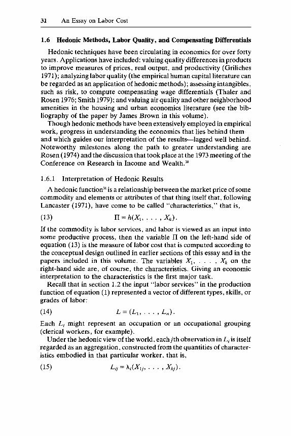
31 An Essay on Labor Cost
1.6 Hedonic Methods, Labor Quality, and Compensating Differentials
Hedonic techniques have been circulating in economics for over forty years. Applications have included: valuing quality differences in products to improve measures of prices, real output, and productivity (Griliches 1971); analyzing labor quality (the empirical human capital literature can be regarded as an application of hedonic methods); assessing intangibles, such as risk, to compute compensating wage differentials (Thaler and Rosen 1976; Smith 1979); and valuing air quality and other neighborhood amenities in the housing and urban economics literature (see the bib- liography of the paper by James Brown in this volume).
Though hedonic methods have been extensively employed in empirical work, progress in understanding the economics that lies behind them- and which guides our interpretation of the results-lagged well behind. Noteworthy milestones along the path to greater understanding are Rosen (1974) and the discussion that tookplace at the 1973 meeting of the Conference on Research in Income and Wealth.M
1.6.1 Interpretation of Hedonic Results
A hedonic function3’ is a relationship between the market price of some commodity and elements or attributes of that thing itself that, following Lancaster (1971), have come to be called “characteristics,” that is,
(13) n = h ( X l , . . . , Xk) .
If the commodity is labor services, and labor is viewed as an input into some productive process, then the variable Il on the left-hand side of equation (13) is the measure of labor cost that is computed according to the conceptual design outlined in earlier sections of this essay and in the papers included in this volume. The variables XI, . . . , X k on the right-hand side are, of course, the characteristics. Giving an economic interpretation to the characteristics is the first major task.
Recall that in section 1.2 the input “labor services” in the production function of equation (1) represented a vector of different types, skills, or grades of labor:
(14) L = (L1, . . . , L J .
Each Li might represent an occupation or an occupational grouping (clerical workers, for example).
Under the hedonic view of the world, eachjth observation in Li is itself regarded as an aggregation, constructed from the quantities of character- istics embodied in that particular worker, that is,
(15) Ljj= Ai(Xi,, . . . , Xk,).

32 Jack E. Triplett
Moreover , the characteristics are the true inputs to the production process. Taking the human capital literature as an example, if years of education and years of experience are productive characteristics of labor type &, then the quantity (years) of education and experience embodied in Li are the inputs entered in the production function, rather than the quantity of Li. A similar interpretation can be given for a hedonic func- tion on consumer goods (where the characteristics of goods are treated as the true arguments of the utility function, not the consumer goods them~elves) .~~ An alternative rationale exists for the characteristics of hedonic functions when the object is to analyze outputs or
It might be true that the productive contribution of each characteristic is independent of the particular Li in which it is embodied, in which case it is not necessary to distinguish between labor types once their characteris- tics have been enumerated. An experienced accountant is simply “more” labor than a beginning machine tender. Much of the labor quality and human capital literature is built on this assumption. More probable, however, are situations in which (say) a year’s experience or education has different productive implications in various occupations, or where characteristics that are important in some occupations are of little or no value in others. In both these cases, occupations matter in the structure of production, and there will be one aggregation rule ( X i in eq. [15]) for each occupation.”
In any event, in the “hedonic hypothesis” the arguments of a hedonic function are, at least in principle, the arguments of either a utility func- tion or a production function, as the case may be, when the hedonic function is viewed from the buyer’s side of the market. This does not, however, imply that the hedonic function is derivable from or directly related to the functions that economic units optimize. The function h in equation (13) is not X i in equation (19, and the one is not a function solely of the other.
Instead, the hedonic function provides an estimate of the constraint on the behavioral unit’s optimization problem. Or, to put it more precisely, those constraints can be derived from hedonic functions, since empiri- cally the forms used to estimate hedonic functions have never explicitly taken on the form of the behavioral constraint.
For simplicity in both the exposition and the economics, assume that the production function of equation (1) contains only one labor type, Li, or that a suitable partitioning exists so that one can consider input Li in isolation from all other inputs. Labor input Li is, however, not ho- mogeneous, as it contains productive characteristics XI and X , in amounts varying with different individuals (an example might be a service industry in which the output of service depends on the years of training and experience of individual workers).
Cost minimization for a producer requires combining productive in-
33 An Essay on Labor Cost
puts in proportions such that ratios of their unit costs equal ratios of their marginal productivities. In the present case, the productive inputs are characteristics XI and X,; a production isoquant for these two inputs can be derived in the regular manner (examples are A and H in fig. 1.1). If XI and X2 are education and experience, the firm’s production problem involves finding an optimal composition of these productive labor-force attributes.
Information on unit factor (characteristic) costs can be obtained from the hedonic function. Still assuming for simplicity only two characteris- tics, the hedonic function of equation (13) can be used to compute
(16) p = p(dX2/dX1, II constant).
The value of the p function of equation (16) gives the relative price of XI in terms of X2 and is computed from the coefficients of the hedonic function of equation (13). Since an isocost curve shows combinations of inputs that can be obtained for the same outlay (and in this case the inputs are characteristics XI and X2) , the p function can be viewed as tracing out an isocost curve, or a portion of one, in characteristics space. One of these is designated as p in figure 1.1. There is one such locus for every value of labor cost for which workers can be hired.
Rosen (1974) emphasizes that the locution of the hedonic function (or, inter alia, of the p function) is determined by all suppliers and demanders in the market, and that it is an envelope of the behavioral functions on both sides of the market. The present section emphasizes a different aspect of that model-the hedonic function as a carrier to the employer of economic information on factor costs. Notation for more than two char- acteristics is obvious, but the extension to cases where capital and mate- rials costs or other labor types are incorporated into the cost minimiza- tion problem is tedious, though not fundamentally different (see Triplett 1982).
1.6.2 Hedonic Methods as Adjustments for Labor Quality
Hedonic functions provide information about the prices or unit costs of characteristics, and therefore about the costs of productive inputs in cases where the characteristics are the inputs to the productive function. This rationale for hedonic functions can be used to motivate their use for adjusting labor cost measures for labor quality. This subject deserves a whole paper on its own. The following is accordingly only an outline of a more comprehensive treatment. Parts of it are adapted from Triplett (1982) and Pollak (1983).
We first develop the notion of labor quality in the context of measuring labor cost. The basic input cost theory outlined in section 1.2 of this essay applies to any definition of a productive input. Accordingly, index num- ber theory can readily be modified to apply to “characteristics space”-

34 Jack E. Triplett
the case where productive inputs are the characteristics of workers- rather than the normal case in which inputs are taken to be quantities of undifferentiated labor hours (sometimes referred to as “goods space”).
Assuming for simplicity that capital and materials are homogeneous goods, and, for the moment, a casual labor market (to avoid the complex- ities of section 1.4), the production function of equation (1) is rewritten as
(17) Q = €?*(K, M7 XI, . e ,
The cost function of equation (2) becomes
(18) C = C* ( R , P, anlaxi, . . . , aII/aX,; Q ) , where C* , the “characteristics production cost function,” is interpreted (as before) as the minimum cost of acquiring a set of inputs sufficient to produce some specified level of Q. Computing equation (18) requires, in addition to the prices of capital and materials, implicit prices for each of the labor characteristics ( X I , . . . , X,) . Hedonic methods are a means for determining those implicit prices, aII//a&.
Just as the input cost index of section 1.2 was computed from the cost function of equation (2), the “characteristics input cost index” is the ratio of values of C* under alternative price regimes (including alternative implicit prices in eq. [13]). A more extensive treatment of the input cost index in characteristics space is given by Triplett (1982).
A change in labor quality is identified with increases or decreases in the quantities of labor characteristics used as inputs in the production pro- cess. In the characteristics input cost index, it is natural to take the notion of labor “quality” as nothing more than a shorthand expression for the quantities of characteristics in the vector X I , . . . , X,. Contrary to presumptions often encountered in the literature, analysis of labor qual- ity does not require any explicit scalar measure of “quality” (such as a “labor quality index,” which in fact provides no additional information).
Shifts in labor characteristics may reflect simple substitution among characteristics in response to changes in relative input prices. The inputs of characteristics included in C* in one period are therefore not exactly the same as in some other period; this, of course, is normal in any input cost index. Thus, when labor quality is identified with the productive labor characteristics, X I , . . . , X,, a “constant quality” input cost index is nothing more than the normal specification of a theoretical input cost index defined on input characteristics-an index in which the inputs (characteristics) included in both periods are the minimum cost set that are sufficient to produce the specified output level, Q. A “constant quality” index is not necessarily one in which there are no changes in labor characteristics.
Of course, when making comparisons of labor cost, the level of output must be held constant. Frequently, one observes changes in labor charac-

35 An Essay on Labor Cost
teristics that are inconsistent with the constant output measurement rule, and, for these cases only, a “labor quality adjustment” must be made. Such an adjustment is interpreted as responding to a change in the characteristics set (XI, . . . , X,) by altering the inputs in Q* in such a way that C* (eq. [MI) refers to the same level of output (a specified value for Q) in both index comparisons.
In the theoretical, or exact, input cost index, the “quality adjustment” may be quite complicated, involving all of the inputs and not just the one whose characteristics actually changed. One also has to consider rather carefully the source of the changes that have been observed, which is equivalent to specifying precisely the question that is being addressed. We leave these complications aside (see Triplett 1982).
Note that in general the “hedonic” or quality adjusted price index cannot be computed from the hedonic function alone. Like any exact index, the Characteristics input cost index requires information from the cost function C*, and hence from Q*, whereas the hedonic function only provides information about a portion of the firm’s isocost line for produc- tive inputs (eq. [16]). The “hedonic price indexes’’ that exist in the literature (see Griliches 1971 and Triplett 1975) are not based on cost functions and are best interpreted as approximations to the true charac- teristics cost indexes, somewhat in the fashion that ordinary fixed-weight price index formulas are thought of as approximations to the true indexes in conventional index number theory.35
In summary, the “constant quality” input cost index is simply the theoretical input cost index defined in characteristics space. I use the term “simply” advisedly. Though simple in concept, such an index requires an enormous amount of information, including not only the characteristics costs, but also the full production or cost function defined on characteris- tics. Its computation involves a host of difficulties (Pollak 1983).
If the production and cost functions are known, then one can possibly use implicit prices obtained from hedonic functions to compute charac- teristics input cost indexes. However, as will be spelled out in section 1.6.3, if production and cost functions on characteristics are not known (the usual case), serious difficulties surround using hedonic prices to estimate them. This implies that estimating the exact input cost index from price and quantity information is not straightforward in a character- istics world (see also Pollak and Wachter 1975).
To this point, the discussion has concerned the cost index for the full set of inputs in equation (17). As noted in section 1.2, a labor cost index is a subindex of the full input cost index. Its construction requires separability conditions on production and/or cost functions. For the characteristics input cost index, the analogous condition specifies that labor characteris- tics (or their unit costs) be separable from capital and materials inputs (or their costs).% If the labor cost subindex exists, it simplifies the quality

36 Jack E. Triplett
problem somewhat because the labor cost index becomes a function only of the arIldx. terms of equation (18) and the level of a “labor aggregator function,” the value of which is held constant over the index comparison. The previous discussion of the meaning and interpretation of quality change and the use of hedonic methods to evaluate it carries over to the labor cost subindex in the form of an extension. However, the required separability conditions for constructing subindexes seem less plausible, if anything, for the labor cost index defined in characteristics space, for they imply that the substitution of (say) education and “raw” labor is indepen- dent of the mix of capital inputs.
In empirical work one seldom has the luxury of working with the theoretical or exact index, for the information requirements of exact indexes are prohibitive. The best one normally has available are indexes constructed as close approximations to the theoretical concept. One criterion of adequacy in an approximation is the extent that the measures take account of, or control for, quality variation.
A curious anomaly of the literature on economic measurement is the disparity that exists between concerns for “quality error” in price and labor cost measures. In the case of price indexes, quality error has long been judged a serious limitation on the validity of empirical measures (Price Statistics Review Committee 1961). On the other hand, taking average hourly earnings (total payrolls divided by hours paid for) or the related hourly compensation series (both are described in Antos, this volume) as a labor cost measure is a common practice that normally raises the most modest of demurrers.
One would judge from the extent of the literature and of professional discussion that the labor market measures were the better of the two. Yet that is clearly not the case. Whatever the quality error remaining in available price indexes (the Consumer Price Index, for example, or the various forms of the Producer Price Index), a great amount of attention is paid to limiting quality variation in price quotes accepted for those indexes, and price indexes have been designed in other ways as well to be far closer than are AHE measures to the concepts needed for economic analysis (Gillingham 1974 describes the use of the cost-of-living index theory as a framework for constructing the Consumer Price Index). By the normal standards applied to price indexes, AHE measures are woefully deficient, essentially because only total establishment payrolls and hours are collected, rather than an earnings or a labor cost concept.
Gollop and Jorgenson, in this volume, are among the few economists to pay serious attention to the labor quality problem. Remarking that AHE or hourly compensation measures “conceal an enormous heter- ogeneity,” they set out to purge them, to the extent possible, of error attributable to their near total lack of control for labor quality shifts. The size of the task Gollop and Jorgenson set for themselves is indicative of

37 An Essay on Labor Cost
the magnitude of the quality problem in normal earnings measures-their data are factored into some 81,000 cells to control for labor quality, roughly 1600 cells per industry.
Gollop and Jorgenson assume an industry labor aggregator function that is translog in form. The traditional rationale for aggregation of this type is to interpret each of the 1600 cells to be a separate factor of production-that is, the vector of labor services in the production func- tion of equation (1) has 1600 elements. Though it is also traditional to assume that labor services are a natural aggregate, the theoretical jus- tification for doing so requires that the cost function (eq. [2]) be separable on these 1600 cells. Evaluating the plausibility of this separability assumption is nearly impossible owing to the sheer mass of data.
The material in this section supplies an alternative rationale. Gollop and Jorgenson’s ten occupational cells are taken as corresponding to the Li categories in equation (14). Age and education (age being a proxy for work experience) within industry-occupation groupings represent labor characteristics-the X’s of equations (13), (15), and (17), and the charac- teristics are the true productive inputs (or are proxies for the true inputs). Further division of these cells by workers’ sex follows precedent in the literature and presumably reflects a correction for omitted characteristics or occupational detail. Under this rationale, the heterogeneity of worker productivity is accounted for by the characteristics, and a labor cost subindex that controls for labor quality can be constructed from the characteristics using the appropriate separability assumptions on equa- tion (18).
Though Gollop and Jorgenson do not formally adopt the rationale presented here, their work is not inconsistent with it. Their procedure amounts to grouping individuals within occupations by the quantities of characteristics embodied in them. This kind of grouping is an alternative to an explicit computation of a characteristics labor cost index. It also corresponds to the way quality change is typically handled in price indexes.
An explicit characteristics-space rationale for work of the Gollop- Jorgenson type has several advantages over the traditional (or “goods- space”) rationale. (1) Testing for functional separability involves only the inputs, age (experience), and education in each Li category, not a set of 1600 inputs. (2) The characteristics variables have an explicit economic justification rather than appearing as ad hoc adjustments, which is the case in traditional treatments. (3) Grouping the characteristics by oc- cupation is supported by the Hicksian aggregation rule outlined in note 34, and those occupational groupings can be tested empirically by straightforward tests on earnings functions; the traditional approach leaves occupational groupings arbitrary, and provides no natural method for testing groupings for realism. (4) Under the characteristics-space
38 Jack E. Triplett
rationale, “quality adjustment” can be incorporated into the theory of production and index numbers in a natural way that permits the analysis of alternatives; the traditional conceptual mode leaves quality change as a mathematical parameter imposed from outside economics whose charac- ter is obscure, properties ambiguous, and identification improbable.”
The Gollop-Jorgenson data base provides researchers for the first time with labor cost measures by industry that are controlled for labor quality variation. It is a particularly valuable contribution in view of the fact that the only government provided labor cost measure that does control for occupational and other shifts (the BLS Employment Cost Index) has little industry detail, which greatly limits its analytical usefulness.
Gollop and Jorgenson follow most studies of labor quality in using some variant of the human capital approach, so the characteristics that are included in the analysis are education and experience measures. This approach has the weight of literature and precedent behind it, yet three reservations should be expressed about the human capital treatment of labor quality.
First, education and experience are not characteristics in the sense that this term was defined and used in equations (13) and (17). Education and experience are not in themselves productive characteristics, but they are proxies, or are associated in some way with skills that are productive or with the acquisition of productive skills. We can think of the true mea- sures as the outputs of processes in which years of education and of experience are the inputs. Of course, the true measures of skills are really wanted in equations (13) and (17), and they would be used there if they were available.%
Second, economists have taken both education and experience as good proxies for productive inputs because both are associated with increases in earnings, and standard theory predicts a relation between variance in wages and a measure of marginal product. However, Lazear (1979) has shown that rising experience-earnings profiles may result when firms and workers make implicit, multiperiod contracts, even if there is no associa- tion between productivity and experience. Lazear and Moore (1981) estimate that only 11 percent of the association between experience and earnings originates from the higher productivity of more experienced workers; the remainder of the rising experience-earnings profile consists of deferred payment incentives under long-term implicit contracts. Ex- perience is undoubtedly more nearly a productive attribute for the youn- ger groups of workers, as Lazear (1976) himself and many other econo- mists have shown. For older workers, use of experience as a labor quality indicator would appear to overadjust labor cost measures for labor quality.
Of course, the implicit contract argument does not invalidate consid- eration of experience variables in measuring labor cost, because one

39 An Essay on Labor Cost
would presumably still want to “standardize” labor cost measures for differing points on the time profile of the implicit contract (see section 1.4). But there is reason to question the traditional view of the economic role of experience, and there is room for a great deal of additional research that will specify the appropriate way of treating experience in the measurement of labor cost, and that will define the variables that do measure productive labor characteristics and can be used for studies of labor quality.
Third, and most important, the human capital view of labor quality has often led to the notion that labor quality is a unique scalar measure and that rankings of workers or groups of workers by some “labor quality index” are useful for comparisons over long time periods or across regions (see Johnson in this volume).
Consideration of equations (17) and (18) suggests that any labor qual- ity measure is some aggregation of labor characteristics, and, as in any aggregation, weights matter. Weights in this case could be marginal products of labor characteristics or the implicit prices of equation (18), in which case the labor quality measure amounts to a quantity index of characteristics. The labor quality measure, in other words, is not a unique scalar measure, but is instead a construction that resembles Gross National Product or any other aggregate quantity measure in which disparate quantity units are combined into some value measure in order to make meaningful economic statements. It has long been understood (see Samuelson and Swamy 1974, and the references cited there) that such quantity measures produce rankings that are not invariant to relative prices; for example, real consumption in Norway may be above that of Costa Rica when valued by one country’s prices, but below when valued by the other’s.
It has not been generally understood that the same principle holds for quality measures. The frontiersman of the last century lacks the skills for success in a modern labor market to the same degree that a computer systems analyst is ill-equipped for the world of Natty Bumppo. Nichols remarks in this volume that today’s unskilled worker would have been regarded as semiskilled at the turn of the century because today’s worker has more education; perhaps so, but many skills that were important then have become obsolete, and we generally lack the information to rank workers of both periods by weighting systems that apply to each period. The habit of taking years of schooling as an invariant measure of labor quality imposes today’s weights on intertemporal comparisons of labor skills and obscures the fact that a comparison from yesterday’s perspec- tive may well reveal the classical “index number problem.”
Even in contemporary comparisons, uncritical application of scalar human capital measures produces potential errors. Layard (1979, p. 52) notes that “college-trained people, if they had not gone to college, would

40 Jack E. Triplett
have earned less than those who did not go to college but had the same measured abilities” (emphasis supplied). If the implicit prices for labor characteristics produced by college were to fall sufficiently (or were lower in some parts of the country than in others), those other, nonmeasured skills possessed by workers who specialize in nonintellectual occupations would be more highly valued by the market, leading to changes in the rank ordering of worker quality.
This analytic problem deserves more attention in the construction of labor quality measures.
1.6.3 IIedonic Methods and the Estimation of Labor Market Differentials
A hedonic function yields an opportunity locus that can be interpreted as a producer’s isocost curve. Having estimated such a thing, it is natural to want to use it for something else. For example, one might wish implicit prices for characteristics for use in explaining demands for those charac- teristics.
In the labor cost context, we might suppose (despite the caveats of the last section) that characteristics are human capital components, such as education and experience. They might also be strength and dexterity, or any other elements that are associated with the productive contribution of the labor input. Equation (13) is estimated as one form of the ordinary “earnings” function. Alternatively and analogously, one may wish to use hedonic prices to estimate consumers’ demands for air quality or other nonmarket goods, starting from a hedonic relation similar to equation (13)’ but involving (say) real estate prices and housing and environmental characteristics. A third example, from the labor economics literature, involves use of hedonic functions to determine wage differentials that compensate workers for risky or unpleasant occupations.
The question we wish to address takes the following form: Under what conditions, if any, can we use the coefficients of the earnings function to explain the firm’s employment of productive characteristics?
One proposal is to estimate the hedonic function (eq. [13]) in the first stage. Next, one estimates the production function of equation (17) or the input demand equations derived from it, in which the labor input is defined by quantities of labor characteristics, and the characteristics implicit prices (aIl/aX1, . . . , aII/dX,) are employed as unit input costs. This is often referred to as the “two-stage’’ proposal and was originally outlined in Rosen (1974).
Figure 1.1 suggests the problems this proposal poses. The p function in figure 1.1 comes from equation (16) and is drawn for a particular value of labor cost. Its slope shows relative implicit prices for labor characteristics XI and X,. Isoquants A and H are portions of production functions of

41 An Essay on Labor Cost
I : \ I I I-
k” H I
I I I I I I I \
a2 X Z
Fig. 1.1
employers A and H. Cost minimization by each results in employment of factor proportions indicated by a and h, respectively.
Suppose initially that nothing was known about the production func- tions, that we merely observe the implicit prices from the p function and the input quantities corresponding to the points a and h. There is in this example variance in relative characteristics prices (slopes of the p func- tion at a and at h), a necessity for an empirical demand study. Moreover, there is also variance in the quantities of characteristics XI and X,. In the absence of information about the shape and position of the production functions, superficial examination of the prices and quantities suggests a situation which, when encountered in “goods space,” signals to the researcher that “all’s well.”
But knowing the production functions in this case reveals that the price

42 Jack E. Triplett
and quantity data have not been generated from the kind of conceptual experiment on which demand theory rests. Differences in the firms’ production functions, stemming from the inherent technology, from entrepreneurial heterogeneity, or whatever, have caused firms A and H to “locate” at different points on the hedonic function. Because the firm in a hedonic world takes the p function as given, and not necessarily the prices, as is the case in the goods world (a point noted by Rosen 1974), it can in a sense choose both p’s and q’s in its cost minimization process.
Thus, variation in characteristics prices and quantities is not sufficient to justify use of characteristics-space data in a demand analysis. The quantity differences between the solutions chosen by firms A and H are not functions of the p function prices alone, and the implicit prices cannot, in a cross-section study, explain differences among firms in the quantities of characteristics employed. Similar points can be made about the use of hedonic prices to explain housing demand.
Before proceeding, several points can be noted about the empirical dilemma portrayed in figure 1.1. First, the dilemma does not rest on nonlinearity of the p function, as figure 1.2 makes clear. Essentially, figure 1.2 presents in characteristics space the empirical fact that has long limited the ability to do cross-section demand studies with data on “goods”-insufficient variance in relative prices.
There is, however, a certain irony to this discussion. The majority of hedonic functions that have actually been estimated have employed functional forms for which the p function is linear. The well-worked semilog functional form, for example, which gives a nonlinear hedonic function, has a linear p Had economists understood that relative characteristics prices were in fact constant for the hedonic func- tions most of them were working with, they might never have set off to try to use hedonic prices in a cross-section demand study in the first place. It is ironic that it took a double misunderstanding about the hedonic framework to generate this research. Nonlinearity in the p function, not nonlinearity of the hedonic function, is the necessary condition for gener- ating variance in relative characteristics prices; however, nonlinearity of the p function is not a sufficient condition to justify the use of hedonic prices in a characteristics demand study.
Second, the research dilemma of figure 1.1 is inherent in the concept of a heterogeneous product. If all demanders were like firm A in figure 1.1, heterogeneous products would either disappear from the market-leav- ing only one outcome (ul, u2) -o r , in the case in which the inputs are supplied in heterogeneous form by act of nature (the labor input), the hedonic function would coincide with firm A’s production isoquant, as noted by Rosen (1974). But in the latter case, no buyer would care which variety was purchased, so no relevant heterogeneity exists, and the goods might as well be treated as homogeneous within price classes.
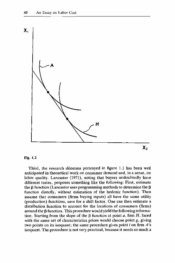
43 An Essay on Labor Cost
Fig. 1.2
Third, the research dilemma portrayed in figure 1.1 has been well anticipated in theoretical work on consumer demand and, in a sense, on labor quality. Lancaster (1971), noting that buyers undoubtedly have different tastes, proposes something like the following: First, estimate the p function (Lancaster uses programming methods to determine the p function directly, without estimation of the hedonic function). Then assume that consumers (firms buying inputs) all have the same utility (production) functions, save for a shift factor. One can then estimate a distribution function to account for the locations of consumers (firms) around the p function. This procedure would yield the following informa- tion. Starting from the slope of the p function at point a, firm H , faced with the same set of characteristics prices would choose point g, giving two points on its isoquant; the same procedure gives point i on firm A’s isoquant. The procedure is not very practical, because it needs so much a
44 Jack E. Triplett
priori specification of the production function that there is little left over to estimate. (Lancaster’s example involves a Cobb-Douglas utility or production function, and there is little need to estimate elasticities in that case.) To my knowledge nothing has come of Lancaster’s suggestion.
That the dilemma of figure 1.1 would emerge in studies on labor quality was also in a sense anticipated in Hicks (1963). Hicks’s hypothesis had the “better quality” employer making better use of the higher quality work- ers. Shifts in demands for worker skill levels might be explained by variations in the skills, education, and training of entrepreneurs, and entrepreneurial characteristics could be taken as the “shift factor” accounting for the distribution of isoquants around the p function in figure 1.1.
The paper by James Brown in this volume explores whether the re- search dilemma of figure 1.1 can be resolved by treating it as some variant of the standard econometric identification problem. In the standard problem, functions such as supply and demand curves can be identified if some variables can be found which are unique to one of the two. Iden- tification permits estimation of the effects of variables which are common to both-price elasticities for supply and demand, for example. In the problem at hand, the effort is to find some variables in the employer’s characteristics demand functions that are not contained in the hedonic functions and that account for the distribution of demanders around the p function, as in figure 1.1.
After considering rather exhaustively a catalog of econometric methods that might identify the production functions from the hedonic functions, Brown finds none that appears very promising. In general, it seems difficult to conceive of a situation in which one can be sure that differences in quantities of characteristics demanded are not attributable to location decisions of demanders around the p function, as well as cost-minimizing reactions to the relative prices themselves. Brown’s con- clusion parallels Pollak and Wachter’s (1975) finding that implicit prices have limited usefulness for explaining outcomes of household production models.
Thus, econometric solutions seem unattainable; the essence of the solution, if the problem is solvable at all, involves generation of an appropriate data set, not elaboration of econometric methods. The way to look at the problem is to ask whether one could plausibly interpret data sets in a way that is consistent with the conceptual experiment that underlies normal demand analysis-that is, can one envision a particular price-quantity data set on characteristics as having been generated by a process of both varying the characteristics prices faced by an individual economic behavioral unit and observing the changed characteristics quantities as responses?
45 An Essay on Labor Cost
To show how hard it is to come up with the required data set, it is worth noting a recent example in which a plausible case was constructed. G. Brown and Mendelsohn (1981) estimated demand for “fishing holes” by characteristics. First, they estimated hedonic functions across various fishing sites to obtain implicit prices for the attributes of each site. Then, on the assumption that fishermen did not choose their place of residence on the basis of proximity to a fishing site, and using transportation expenses from home to site as an element of the cost of the fishing expedition, they constructed, essentially, figure 1.3. In this case, because the distance to the site was a unique element in the hedonic function for each fisherman, they were able to estimate fishermen’s demands for different characteristics of fishing spots, an accomplishment of consid- erable ingenuity which will undoubtedly be a substantial service to plan- ning outdoor recreation facilities. However, the fact that the Brown- Mendelssohn data set relates to a problem that is of considerably less than universal interest among economists is probably no coincidence. It is an ingenious solution to a very special problem, and although it may suggest equally ingenious solutions to others, prospects are not high for generat- ing appropriate data sets with more widespread applications.
One should, however, put all this in proper perspective. First, the research dilemma protrayed in figure 1.1 greatly limits the usefulness for behavioral studies of hedonic estimates of implicit prices, but it does not imply that they are useless. Thaler and Rosen (1976), fully recognizing the locational choice problem of figure 1.1, use it to specify that their estimates of the compensating wage differential for risk were a limit (a lower one in their case) on the true estimates: in figure 1.1 terms, the price of XI necessary to induce H to employ al units of XI is far lower than what is required to induce A to locate at that point, and accordingly, A requires less than H to “compensate” for locating in the vicinity of al. Fully understanding the nature of hedonic prices facilitates using them in appropriate ways.
Second, the conceptual problems we have been discussing are merely characteristics-space forms of problems that are ancient in normal goods- space demand analysis. For example, it has long been known that there are regional differences in food prices and consumption. Taking regional variations as appropriate data for demand analysis requires the assump- tion of common utility functions-that regional consumption differences do not reflect regional differences in tastes. Thus, strong assumptions are always necessary to justify using cross-section data in demand analysis. These problems are so timeworn that they are frequently ignored in empirical applications in goods space. Only because working in charac- teristics space is new do the problems discussed in this section seem novel.
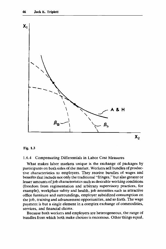
46 Jack E. Triplett
4
A & H
Fig. 1.3
1.6.4
What makes labor markets unique is the exchange of packages by participants on both sides of the market. Workers sell bundles of produc- tive characteristics to employers. They receive bundles of wages and benefits that include not only the traditional “fringes,” but also greater or lesser amounts of job characteristics such as desirable working conditions (freedom from regimentation and arbitrary supervisory practices, for example), workplace safety and health, job amenities such as attractive office furniture and surroundings, employer subsidized consumption on the job, training and advancement opportunities, and so forth. The wage payment is but a single element in a complex exchange of commodities, services, and financial claims.
Because both workers and employers are heterogeneous, the range of bundles from which both make choices is enormous. Other things equal,
Compensating Differentials in Labor Cost Measures

47 An Essay on Labor Cost
variation in one element of either bundle will be offset by equivalent variations in other elements.” If the wage is the element of the compensa- tion package that offsets variation in some other element, or the net effect of a group of elements, then labor markets will exhibit a set of “compensating wage differentials” that reflect worker valuations on everything from a favorable climate to employer subsidized lunches to the aversion many workers have to working for very large employers (Oi, this volume). Considerable research on compensating differentials has been undertaken in recent years (see the bibliographies in Smith 1979 and C. Brown 1980).
The model underlying compensating wage differentials is basically the wage-benefit model of equations (3)-(8). As an example, consider job safety which can be viewed as a benefit (Thaler and Rosen 1976; Sider 1981). Workers will choose less safe jobs only when employers pay a higher wage to compensate them for the risk of injury (eq. [sa]). Alterna- tively, the employer can invest in safety equipment; this will reduce the wage premium that must be paid, and the “amount” of safety that will be provided by market mechanisms will be determined by equation (8).41
Notice, however, an anomaly: If the employer “pays” for workplace hazards in the form of higher wages, it will be recorded in his labor cost data. Dealing with work hazards through purchase of safety equipment will, in most accounting systems, show up as an increase in the quantity of capital equipment. Since both compensating wage payments and expend- itures for safety equipment are necessary because risk creates disutility for workers, both costs need to be considered in labor cost measures on a comparable basis.
The same point can be made about many other nonpecuniary job attributes. Increases or decreases in them may imply changes in the level of wages that must be paid, but there will be concomitant increases in expenditures on other factors, so that considering only those expendi- tures that are explicit to labor misses labor cost that shows up in the form of employer expenditure on some other input.
Positive or negative nonpecuniary elements may be provided by a third party, such as government or an act of nature. Employers who gain (or lose) by receiving (or not receiving) these “free” job characteristics will adjust wages accordingly. For example, the interarea labor cost compari- sons conducted by Johnson (in this volume) control for differences in worker quality among areas; but that, though vital, is only one side of the story. Perhaps both union and nonunion wages are high in Detroit not because of the direct and indirect effects of union power but because of Detroit’s amenity levels relative to competitive areas. Comparisons of labor payments among employers who receive differential benefits by act of government or nature may yield misleading information about the true levels of labor cost.

48 Jack E. Triplett
To make things more difficult for measurement, it may not be possible to separate out of the employer’s total cost structure those aspects which are uniquely associated with the benefit that workers get from an amenity provided by a third party. Roback (1982) shows that when an amenity (for example, a favorable climate) is both desired by workers and inde- pendently productive to firms, then the effect on land rents can be determined, but one cannot tell the direction of the effect on wages. In seeking to allow for the effects of amenities in the labor cost measure- ment, we lack even the clue of sign that will tell us whether estimated values of regional amenities are reasonable or not.
The existence of compensating wage differentials thus means that a unique measure of labor cost may not be extractable from the employer’s total input cost, because the level of labor cost is not independent of the quantity of capital or of some other input. Compensating differentials may also imply that the cost function is not separable on its labor compo- nent (see section 1.2), because safety hazards, for example, are likely to differ among occupations, and adding safety equipment will change the occupational wage structure. But the separability property relates to aggregation; the dependence of labor cost on the quantity of capital in the presence of compensating differentials would be true even if the produc- tion function contained only one type of homogeneous labor. Thus, the challenge raised to labor cost measures by compensating wage differen- tials encompasses, but goes beyond, the classical separability issue.
This problem is unique to labor input to production and occurs because each party to a labor market transaction cares about the characteristics of the other party. There are some other markets for which this is also a fact-rental housing is one clear example. But the problem seems far more pervasive and far more important in measuring the cost of the labor input than for any other productive input, and it is considerably more important than is the case for most consumer goods markets. Measuring labor cost is hardly a simple economic task.
1.7 Conclusions
This essay has addressed the problem of producing a conceptual framework for measuring labor cost that reflects a modern view of the operation of labor markets. The theory of labor cost that is derived from the stylized model of production on which the theory of economic measurement is based (section 1.2) has the following properties that are inconsistent with empirical knowledge of labor markets:
1. Unit factor cost consists exclusively of money wage payments. 2. The labor unit is homogeneous. 3. A casual labor market prevails.
49 An Essay on Labor Cost
4. Production costs can be separated uniquely into labor cost compo- nents and costs of other inputs. Relaxing the first two restrictive properties of the stylized model in-
volves difficult empirical and data development tasks, but does not challenge the fundamental validity of the labor cost measure. Adding costs of benefits clearly is required to reach an adequate measure of labor cost for nearly any purpose (section 1.3). And though there are more conceptual difficulties in measuring some of these benefits than first meets the eye, for the majority of them the measurement can be done within the traditional production theoretic context.
Similarly, dealing with worker heterogeneity can be handled theoret- ically by modeling the productive characteristics of workers and by extending the basic theory of index number measurements into charac- teristics space (section 1.6). The formidable conceptual and theoretical problems that remain cannot be denied. But those pale beside the empiri- cal and data base requirements that have inhibited progress on the analysis of heterogeneity in both goods and labor markets.
Far deeper conceptual problems surround the other two major points discussed in this essay, for they call into question whether a one-period measure of labor cost, or indeed a measure of labor cost at all, is either appropriate or achievable.
Because casual labor markets seldom obtain in the modern economy, employment decisions are not based on a single period’s labor cost (section 1.4), and for the cost concept that is relevant to employers’ decisions, the single period labor cost is not well defined. The identical problem has been discussed in the literature on the measurement of capital and of consumer prices, so it is known to require information about future prices or expected prices. The problem is no more and no less difficult when the objective is measuring labor cost, but the important point is that this serious difficulty be recognized.
Whether a single period measure is relevant or not, perhaps the most basic question to the entire inquiry is whether a labor cost measure can be distinguished uniquely from a measure of all input costs. In the stylized model, this issue takes the form of an empirical question about cost function separability (section 1.2), but in this there is nothing unique to labor input; the technical issue of separability can be raised about any class of inputs, from lubricants to office supplies. What makes the labor input uniquely difficult is that the seller of labor cares not just about the wage but also about employment conditions and other characteristics of the buyer. Because there is so much employer heterogeneity, the variety in compensation packages will be great. And variation in elements of the compensation package leads to variation in the quantities of other inputs, especially capital. This dependence between quantities of one input and

50 Jack E. Triplett
“prices” paid for another poses special and very difficult problems for the measurement of labor cost.
This essay began with the observation that labor economists tended to view the subject as too difficult because of the institutional detail, while theorists thought it conceptually too simple to be worth much attention. It concludes with the observation that-whatever the jungle of institu- tional detail that must be considered-the greatest difficulties are concep- tual ones. That, of course, is why economists should find the subject interesting.
Notes 1. The theory of consumption price measurement stretches back to Wicksell, but see
Fisher and Shell (1972), Pollak (1971), Samuelson and Swamy (1974), Diewert (1976), Blackorby, Primont, and Russell (1978), and Deaton and Muellbauer (1980). A survey of empirical studies in price measurement is Triplett (1975). See also Griliches (1971).
2. Information sources for the surveys cited include: Center for Human Resource Research (1975) for NU; Duncan and Morgan (1975) for PSID; Rees (1974), Kehrer (1979), and Spiegleman and Yeager (1980) for the Income Maintenance Experiments; Mellow (1981) and U.S. Department of Labor (1980) for CPS data.
3. Though I believe there is no question that the demand side of labor economics has been neglected, the habit of thinking only in supply-side terms is so ingrained that experi- ence shows I should present an example to support the statements in the text. The regional wage differential literature in labor economics will serve.
Johnson, in this volume, notes a “current consensus” that a North-South differential exists in nominal wages, but not in real wages; the literature he cites and the model of his paper take these putative facts as consistent with labor market equilibrium: “. . . other things equal, a 1 percent increase in the cost of living in an area willincrease the equilibrium wage in that area by 1 percent” (Johnson, this volume, p. 311). But a nominal wage differential implies a production cost differential, and, if employer mobility exists, will provoke interregional movement of employers, unless somehow the wage differential is offset by cost differentials for other factors (highly unlikely if there are opportunities for employer specialization). Equivalence between nominal wage and cost-of-living differen- tials is consistent only with predictions from the theory of worker behavior and is not consistent with general equilibrium at all. In fact, an empirical finding so extraordinarily inconsistent with theoretical prediction is suspect; if it were true, it ought to suggest a vigorous research effort to determine why. Instead, it seems to be an article of faith that nominal wage differentials, when found, can be “explained” by living cost differentials. For a more balanced view of regional differentials, see Hanushek (1981); the regional eco- nomics literature has also treated economic differentials from an alternative perspective (see the items cited by Muth, this volume).
4. It is astonishing, but nevertheless true, that at this date one still has to defend the use of measurement theory in formulating economic measurements, even among researchers who comfortably use labor market theory for other purposes. One can only guess about the reasons for such an anachronism, but one possibility is the relative lack of understanding, even among sophisticated data users, of the conceptual complexity of some of the issues that arise in the construction of economic data combined with impatience with theoretical work that does not produce immediately usable “answers.” The main use of theory in economic
51 An Essay on Labor Cost
measurement is to sharpen measurement concepts and to provide an integrated framework against which consistent resolution of practical measurement problems can be assured. To be useful, the theory need not-and seldom does-provide ready “cookbook” guidance for measurement decisions. Its role is comparable to John Maynard Keynes’s description of the relation between economic analysis and economic policy:
The Theory of Economics does not furnish a body of settled conclusions immediately applicable to policy. It is a method rather than a doctrine, an apparatus of the mind, a technique of thinking, which helps its possessor to draw correct conclusions. (as quoted in Reder 1982, p. 16)
The use of theory in measurement does not assure that the measurements will always be correct, but experience has shown that the alternative produces ad hoc, inconsistent, and ultimately indefensible decisions.
5 . Terminology is not uniform in the literature in part because the explicit literature on the theory of input price measurement is sparse. Caves, Christensen, and Diewert (1982) employ the term “Malmquist index” of input prices. Also, an “input cost index” sometimes refers to a computation intended as a proxy for an output price index (a weighted average of wage rates and materials prices, for example, in lieu of a measure of the price of construc- tion), but that is not the purpose of the measurement discussed in this essay.
6. Actually only their factor quantity index numbers are explicitly based on the translog model; their factor price indexes are defined implicitly with respect to this model and are not derived (as exact input cost indexes would be) from the cost function that is associated with their production model. There is little reason for supposing this makes much difference in their labor cost measures. Deriving the labor cost indexes from the cost function that is dual to the translog production model would be prohibitively expensive, owing to properties of the translog model that, in general, assure that factor quantity and factor price indexes have different functional forms. For the theoretical statement of these issues, see Samuelson and Swamy (1974) and Diewert (1980).
7. Braithwait (1980) found that the Laspeyres index differed from exact indexes of consumption prices by only about one-tenth of an index point per year, a result compatible with estimates in Christensen and Manser (1976) and Goldberger and Gameletsos (1970). Diewert (1976) and Caves, Christensen, and Diewert (1982) show theoretically that certain types of conventional index number formulas will give close approximations to exact indexes.
8. “Roughly” because separability of the cost function is equivalent to comparable separability of the production function only for certain production function forms, not all of them. See Blackorby, Primont, and Russell (1978).
9. The appropriateness of the Grant and Hamermesh approach requires interpreting their demographic groupings as proxies for distinct inputs to the production process-that is, if occupations, skill levels, or other characteristics actually define categories of labor input (the Lls of eq. [14]), one must assume that these characteristics vary by age, sex, and race in such a way that the latter identify, at least partly, the former. See the discussion of this point in section 1.6.2.
10. The parameter JI indicates the rate of exchange between benefits and wages on the boundary of the worker’s choice set. It can be identified as a locational parameter selected from a hedonic frontier (see section 1.6.3, and also Atrostic 1982, who implements a similar approach empirically). Competition will tend to bring JI into equality both with the price at which workers could buy benefits on the market and with the employer’s marginal cost of providing them (see eq. [S]), and for this reason the price of benefits has often been assumed to be one or the other. Taking the market price of benefits as the value of JI, however, introduces the implicit assumption that the worker can sell them, which is generally untrue. Setting JI identically equal to the employer’s marginal cost of providing benefits is likewise inappropriate, because benefits are presumably provided when the worker places a higher
52 Jack E. Triplett
value on inframarginal units of them than it costs the employer to provide them. Assuming in the worker’s full income constraint that + is measured by either the market price of benefits or the employer’s cost of providing them improperly introduces elements of the solution to a maximization problem into the constraint that bounds the problem. Put another way, this assumption amounts to specifying that equation (8) is identically true for all levels of benefits, when in fact equation (8) holds only for the benefit level that corresponds to the cost minimizing and utility maximizing employer-employee contract point.
11. Labor supply to a firm is composed of an hours of work decision and a choice of employer. Equation (4) does not necessarily require that workers have different labor supply responses to wages than to benefits, though the results of Atrostic (1982) suggest this to be the case. It does imply that, once in the labor market, workers will choose among alternative employers according to their preferences among employer provided benefits and market purchased consumption goods. Moreover, the choice of employer (and therefore the employer’s task of selecting an appropriate package of wages and benefits) is not trivial, since alternative compensation packages are available in the market either because em- ployers have different relative costs of providing various benefits, or because workers have different preferences for benefits, or both. See Antos and Rosen (1974).
12. Freeman (1981) discusses the case in which there are start-up costs for offering a benefit to employees, which introduces another term on the right-hand side of equation (8). This has no effect on the results and is ignored here for simplicity.
13. Some researchers (including Smeeding in this volume and Woodbury 1981), reason- ing that because benefits are not taxed they are worth more to workers, have used the marginal tax rate to inflate the value of benefits, rather than reducing the quantity of goods that can be purchased out of wage income (as suggested in the text and as incorporated into the work of Leibowitz in this volume). This practice seems to reflect the habit of writing wages as an argument of the utility function instead of (or as a proxy for) the market purchased goods that belong there, and of omitting either one equation (typically the demand for leisure) or one price (usually consumption goods) from the system being analyzed. In some cases the only objection to the alternative treatment is that it lacks elegance; in others, however, errors result, as David points out in his comment in this volume, because the lack of clarity obscures mistakes in logic.
14. David, in this volume, makes the excellent point that the marginal tax rate will in the long run itself be a function of the proportion of income taken in the form of benefits (because tax rates will be adjusted upward to recoup the revenue loss). This means that taxes will only affect the consumption of benefits of the average worker if there is some sort of money illusion; but because the growth of nontaxable benefits shifts tax burdens toward lower income workers, the main effect of nontaxable benefits may be on income distribution and not on the average consumption of benefits and market purchased goods.
15. Freeman (1981) presents five possible reasons, but the only one I find logically supportable is the possibility that workers can have more faith that benefit plans are sound when a union acts as their agent to oversee them and would, accordingly, be more willing to trade wages for benefits in unionized firms. This motivation seems inadequate to account for the size of the union-nonunion differential in benefits.
16. Atrostic (1981) presents findings that suggest the “single parent” model predomi- nates: Other things equal, female dominated workplaces have higher levels of benefits.
17. For the policy relevance of the elasticity of demand for labor, see Solow’s (1980) presidential address.
18. See the table on p. 504 of Freeman (1981). The difference between the two estimates reported in the text is statistically significant at the .01 level.
19. I form this estimate from comparing the ECNT (which includes an estimate of hiring, training, and turnover costs) and COSTWK measures of table C.2 in Appendix C of this volume. The comparable figure for manufacturing in 1978 was 13-14 percent.
53 An Essay on Labor Cost
20. Oi cites J. M. Clark. Morgenstern (1963, p. 186) includes the “value of tenure” as an
21. This error is implied by Okun’s discussion of Oi’s work (Okun 1981, pp. 17, 24). 22. On the other hand, I do not understand Lazear’s words, “without counting the
output of the human capital,” that follow the passage quoted. Because firm-specific human capital is by definition useful only to the firm itself, its production can only be regarded as an intermediate input for the firm in question; thus, it is not failing to account for its output in equation (12) that leads to the error, but inappropriately accounting for its inpur in equation
element of labor cost.
(11). 23. Hamermesh’s data series are reproduced in Appendix C. 24. This explanation has an ancient history. However, my own observation, from a
relatively short tenure as a construction worker quite a number of years ago, is that the trade attracts individuals who have strong preferences for consuming leisure in concentrated and uninterrupted blocks of time. Thus, construction workers tend to be those for whom employment interruptions require the smallest premiums (Thaler and Rosen 1976 make the same point in a different context). The compensating wage differential explanation may be only part of the reason why construction wages have traditionally been higher than in alternative employments.
25. Some contracts make it clear that the incentive for entering into the contract came from the other side of the market and that what was wanted was assured demand.
26. Diewert (1980, p. 475) writes: “In the previous section I may have left the impression that from a theoretical point of view constructing a capital aggregate is no more difficult than constructing a labor aggregate.” He then proceeds to list and discuss complexities that make capital measurement a particularly difficult problem, including price expectations, interest and depreciation rates, treatment of taxes, definition of the capital input, time period for measurement, choice of index numbers, and so forth. Since most of this catalog of the “special problems” of capital measurement appear in some form in this essay as problems of labor cost measurement, I would modify Diewert’s statement to read: “From a modern understanding of the labor market, constructing a labor aggregate is little, if any, less difficult than constructing a capital aggregate.”
27. See references in note 2. 28. Seiler (1982) reports that a compensating differential for earnings uncertainty
accounts for up to 50 percent of the higher earnings of incentive pay workers in some occupations in the industries he studied, though the average appears to be substantially lower.
29. Lazear (1981) notes that piece-rate compensation is the extreme case of a short-run labor contract, in which workers are compensated only for current period output. In normal cases, a worker’s current period compensation is at least in part a reward for performance in past periods. Piece-rate payment systems will evolve when the costs of supervision are high.
30. Terleckyj (1976), particularly the articles by Ohta-Griliches, King, and Triplett, with the discussion by Barzel and Ingram.
31. This section is based in part on Triplett (1976), modified to apply to labor markets. 32. In Triplett (1976) I introduced the device of characterizing hedonic transactions in
consumer goods as if consumers purchased groceries in preloaded carts, with prices attached to the carts. The preloaded carts play the role of conventional goods, variations in the assortments of groceries they contain amount to quality differences as we usually think of them, and the quantities of the various groceries are the characteristics. The characteris- tics (groceries) are, of course, the true arguments of the utility function, not the goods (the preloaded carts). Estimating hedonic functions on the preloaded grocery carts is equivalent to determining the prices charged for the individual grocery items. The price attached to the cart is simply total expenditures on the groceries contained in it. The grocery cart simile carries over by analogy to the case of labor input.
33. In the supplier case, the characteristics are viewed as joint outputs of a productive

54 Jack E. Triplett
process. Implications of this approach in the context of measuring output and productivity are discussed in Triplett (1982).
34. Both cases imply that hedonic functions will differ by occupation, either in the coefficients (implicit prices) on the characteristics they have in common, or in differing lists of characteristics included in them. In the consumption case, I have suggested (Triplett 1971) that testing for equivalence of hedonic functions across commodity groupings is one way of resolving the old empirical problem: “What is a product?” The extension of that idea to the labor market implies that hedonic functions can in principle be used to distinguish between groups of workers who are appropriately classified as separate factors of produc- tion, as distinct from other groupings that may represent differing qualities of what is essentially the same productive factor. Clerical workers or blue-collar workers are appropri- ate empirical groupings if a single hedonic function describes all the workers in the group; if not, one tests lower level aggregations, such as secretaries or machinists. This empirical rule using hedonic functions amounts to an extension of Hicksian aggregation theorems into characteristics space, since in effect the “rule” permits aggregation over characteristics so long as characteristics prices (the hedonic coefficients) move together in the cross section. This proposal is quite different from that of Cain, Hansen, and Weisbrod (1967) and offers substantial empirical advantages for testing existing occupational classifications for eco- nomic relevance.
35. The literature contains an enormous amount of confusion about the relation be- tween empirical “hedonic price indexes” and the exact or theoretical price index. The usual source of confusion is the failure to distinguish between the hedonic function itself (eq. (131) or its derivative, the p function of equation (16), aqd the characteristics input cost index based on equation (18). This confusion has led to the misguided attempt to derive the former from the latter, or to use the functional form of the production or cost function to derive permissible functional forms for the hedonic function-as, for example, in Lucas (1975) and Muellbauer (1974). Since articles of this genre seem always to conclude (incor- rectly) that the well-worked semilog form is impermissible for hedonic functions, it is worth emphasizing that the functional form of the p function, and hence of the hedonic function itself, is independent of the form of production, cost, or utility functions and is wholly an empirical matter. Assertions to the contrary by Lucas and Muellbauer are really statements that the cost function of equation (18) cannot adequately be represented by a semilog function, a fact that is well known; the form of equation (18) says nothing about the form of the hedonic function.
36. The parentheses make explicit reference to the distinction between direct and indirect separability. See note 8.
37. Fisher and Shell (1972) present an insightful analysis of quality change from the traditional view that probably extracts as much from that approach as can be obtained. Nevertheless, their discussion of “parametrizable” quality change has limited applicability to empirical work and leaves the nature of quality change so obscure that its parameter cannot be distinguished from technical change that shifts the production function.
38. The empirical use of proxy variables and proxy relations is not restricted to labor market hedonic functions; it is an integral part of the empirical tradition of hedonic functions in product markets, where the problems created by the use of proxies are well known (Triplett 1969).
39. If
In II = po + PIX, + pzX2 + e , then a x , l a x , (In II = const.) = p2/pI,
which is clearly a constant for all XI and X,. Thus, the semilog function yields a linear p function, which means it is linear in what might be called the relative price dimension, which is the one that matters most for doing demand analysis. That all aln II/aXj are increasing within the semilog form means that increasing outlays on characteristics imply increasing

55 An Essay on Labor Cost
unit characteristics costs, when the characteristics are purchased in a single “package.” See Triplett (1976) for further discussion.
40. The uniqueness of both worker and employer does present the possibility that workers will be assigned among employers in such a manner that each will be located in a uniquely “best” job match. If so, none of the available alternative job opportunities for a particular worker will offer an exactly equivalent bundle of job characteristics, and no other worker will be quite so satisfactory for the employer. But given a large enough number of employers and workers, unique assignments will create only small deviations and the statement in the text will be approximately true.
41. Because this example is intended only to be illustrative, and then only for labor cost measurement, there is no need to discuss the numerous caveats that would be necessary for a serious analysis of safety. In particular, there is nothing in equation (8) that shows that the amount of safety provided by the market is the “right” amount by some criterion, or that shows that workers can always correctly judge differences in safety between similar jobs, or that pertains to any of the issues surrounding the regulation of workplace health and safety. See Thaler and Rosen (1976).
References Antos, Joseph R., and Sherwin Rosen. 1974. Discrimination in the
market for public school teachers. Journal of Econometrics 3: 123-50. Atrostic, B. K. 1981. Alternative pay measures and labor market dif-
ferentials. BLS Working Paper 127. Washington, D.C.: U.S. Bureau of Labor Statistics.
. 1982. The demand for leisure and nonpecuniary job characteris- tics. American Economic Review 72: 428-40.
Azariadis, Costas. 1975. Implicit contracts and underemployment equilibria. Journal of Political Economy 83: 1183-1202.
Baily, Martin N. 1974. Wages and employment under uncertain demand. Review of Economic Studies 41: 37-50.
Barzel, Yoram. 1976. Comment on “Automobile prices revisited: Exten- sions of the hedonic hypothesis.” In Terleckyj 1976.
Berndt, Ernst R., and Laurits R. Christensen. 1973. The specification of technology in U.S. manufacturing. BLS Working Paper 18. Washing- ton, D.C.: U.S. Bureau of Labor Statistics.
. 1974 Testing for the existence of a consistent aggregate index of labor inputs. American Economic Review 64: 391-404.
Blackorby, Charles, Daniel Primont, and R. Robert Russell. 1978. Dual- ity, separability, and functional structure: Theory and economic ap- plications. New York: North-Holland.
Braithwait, Steven D. 1980. The substitution bias of the Laspeyres price index: An analysis using estimated cost-of-living indexes. American Economic Review 70: 64-77.
Brown, Charles. 1980. Equalizing differences in the labor market. Quarterly Journal of Economics 94: 113-33.
Brown, Gardner, and Robert Mendelsohn. 1981. Hedonic demand func-

56 Jack E. Triplett
tions with linear and nonlinear budget constraints. University of Washington Discussion Paper 81-12. Seattle, Wash. : University of Washington.
Cain, Glen, W. Lee Hansen, and Burton A. Weisbrod. 1957. Occupa- tional classification: An economic approach. Monthly Labor Review
Caves, Douglas W., Laurits R. Christensen, and W. Erwin Diewert. 1982. The economic theory of index numbers and the measurement of input, output, and productivity. Econometrica 50: 1393-1414.
Center for Human Resource Research. 1975. The national longitudinal surveys handbook. College of Administrative Science, The Ohio State University.
Christensen, Laurits R., and Marilyn E. Manser. 1976. Cost-of-living indexes and price indexes for U.S. meat and produce, 1947-1971. In Terleckyj 1976.
Cleeton, David L. 1982. The theory of real wage indices. American Economic Review 72: 214-25.
Deaton, Angus, and John Muellbauer. 1980. Economics and consumer behavior. New York: Cambridge University Press.
Diewert, W. E. 1976. Exact and superlative index numbers. Journal of Econometrics 4: 115-45.
. 1980. Aggregation problems in the measurement of capital. In Usher 1980.
. 1981. The economic theory of index numbers: A survey. In Essays in the theory and measurement of consumer behavior in honour of Sir Richard Stone, ed. Angus Deaton, 163-208. Cambridge Uni- versity Press.
Duncan, Greg J. 1976. Earnings functions and nonpecuniary benefits. Journal of Human Resources 11: 462-83.
Duncan, Greg J., and James N. Morgan, eds. 1975. Five thousand American families-patterns of economic progress, vol. 3. Ann Arbor, Mich.: The Institute for Social Research, The University of Michigan.
Duncan, Greg J., and Frank Stafford. 1980. Do union members receive compensating wage differentials? American Economic Review 70:
Dunlop, John T. 1977. Policy decisions and research in economics and industrial relations. Industrial and Labor Relations Review 30: 275-82.
Ehrenberg, Ronald G., Daniel S. Hamermesh, and George E. Johnson. 1977. Comment. Industrial and Labor Relations Review 31: 10-13.
Feldstein, Martin. 1976. Temporary layoffs in the theory of unemploy- ment. Journal of Political Economy 84: 937-58.
Fisher, Franklin, and Karl Shell. 1972. The economic theory of price indices: Two essays on the effects of taste, quality, and technological change. New York: Academic Press.
90: 48-52.
353-71.
57 An Essay on Labor Cost
Fleisher, Belton M., and Thomas J. Kniesner. 1980. Laboreconomics. 2d ed. Englewood Cliffs, N.J.: Prentice-Hall, Inc.
Freeman, Richard B. 1981. The effect of unionism on fringe benefits. Industrial and Labor Relations Review 34: 489-509.
Gillingham, Robert F. 1974. A conceptual framework for the consumer price index. In Proceedings of the business and economic statistics section, 246-52. Washington, D.C.: American Statistical Association.
. 1983. Measuring the cost of shelter for homeowners: Theoretical and empirical considerations. Review of Economics and Statistics, forthcoming.
Goldberger, Arthur S., and Theodore Gameletsos. 1970. A cross- country comparison of consumer expenditure patterns. European Eco- nomic Review 1: 357-400.
Gollop, Frank M., and Dale W. Jorgenson. 1980. U.S. productivity growth by industry. In New developments in productivity measurement and analysis, ed. J. W. Kendrick and B. Vaccara. Conference on Research in Income and Wealth: Studies in Income and Wealth, vol. 44. Chicago, Ill.: University of Chicago Press for the National Bureau of Economic Research.
Gordon, Donald F. 1974. A neo-classical theory of Keynesian unemploy- ment. Economic Inquiry 12: 431-59.
Grant, James, and Daniel S. Hamermesh. 1981. Labor market competi- tion among youths, white women, and others. Review of Economics and Statistics 63: 354-60.
Griliches, Zvi, ed. 1971. Price indexes and quality change: Studies in new methods of measurement. Cambridge, Mass. : Harvard University Press.
. 1977. Estimating the returns to schooling: Some econometric problems. Econometrica 45: 1-22.
Hall, Robert E. 1982. The importance of lifetime jobs in the U.S. economy. American Economic Review 72: 716-24.
Hanushek, Eric A, 1981. Alternative models of earnings determination and labor market structures. Journal of Human Resources 16: 238-59.
Hicks, John R. 1963. The theory of wages. 2d ed. London: Macmillan. Ingram, Gregory. 1976. Comments on “The demand for housing: Inte-
grating the roles of journey-to-work, neighborhood quality, and prices.” In Terleckyj 1976.
International Labor Office. 1979. An integrated system of wages statistics: A manual on methods. Geneva: International Labor Office.
Katz, Arnold, and Joseph E. Hight, eds. 1977. The economics of unem- ployment insurance: A symposium. Industrial and Labor Relations Review 30: 431-526.
Kehrer, Kenneth C. 1979. The Gary income maintenance experiment: Introduction. Journal of Human Resources 14: 431-33.

58 Jack E. Triplett
King, A. Thomas. 1976. The demand for housing: Integrating the roles of journey-to-work, neighborhood quality, and prices. In Terleckyj 1976.
Lancaster, Kelvin. 1971. Consumer demand: A new approach. New York: Columbia University Press.
Layard, Richard. 1979. Introduction. Journal of Political Economy 87:
Lazear, Edward P. 1976. Age, experience, and wage growth. American Economic Review 66: 548-58.
. 1979. Why is there mandatory retirement? Journal of Political Economy 87: 1261-84.
. 1981. Agency, earnings profiles, productivity, and hours restric- tions. American Economic Review 71: 606-20,
Lazear, Edward P., and Robert L. Moore. 1981. Incentives, productiv- ity, and long-term labor contracts. Paper read at the annual meeting of the Western Economic Association.
Lucas, R. E. B. 1975. Hedonic price functions. Economic Inquiry 13:
Mellow, Wesley. 1981. Unionism and wages: A longitudinal analysis. Review of Economics and Statistics 63: 43-52.
. 1982. Employer size and wages. Review of Economics and Statis- tics 64: 495-501.
Mincer, Jacob. 1974. Schooling, experience, and earnings. New York: National Bureau of Economic Research.
Mitchell, Olivia S., and Emily S. Andrews. 1981. Scale economies in private multi-employer pension systems. Zndustrial and Labor Rela- tions Review 34: 522-30.
Morgenstern, Oskar. 1963. On the accuracy of economic observations. 2d ed. Princeton, N. J.: Princeton University Press.
Muellbauer, John. 1974. Household production theory, quality, and the “hedonic technique. ” American Economic Review 64: 977-94.
Muth, Richard F. 1974. Moving costs and housing expenditure. Journal of Urban Economics 1: 108-25.
Ohta, Makoto, and Zvi Griliches. 1976. Automobile prices revisited: Extensions of the hedonic hypothesis. In Terleckyj 1976.
Oi, Walter Y. 1962. Labor as a quasi-fixed factor. Journal of Political Economy 70: 538-55.
Okun, Arthur M. 1981. Prices and quantities: A macroeconomic analysis. Washington, D.C. : The Brookings Institution.
Pencavel, John H. 1977. Constant-utility index numbers of real wages. American Economic Review 67: 91-100.
Phelps, Edmund S. et al. 1970. Microeconomic foundations of employ- ment and inflation theory. New York: W. W. Norton.
Pollak, Robert A. 1971. The theory of the cost of living index. BLS Working Paper 11. Washington, D.C.: U.S. Bureau of Labor Statis- tics.
S1-S.
157-78.
59 An Essay on Labor Cost
. 1975a. Subindexes of the cost of living. International Economic Review 16: 135-50.
. 1975b. The intertemporal cost of living index. Annals of Eco- nomic and Social Measurement 4: 179-95.
. 1983. The treatment of “quality” in the cost of living index. Journal of Public Economics, forthcoming.
Pollak, Robert A., and Michael L. Wachter. 1975. The relevance of the household production function and its implications for the allocation of time. Journal of Political Economy 83: 255-77.
Price Statistics Review Committee. 1961. The price statistics of the federal government. In U.S. Congress, Joint Economic Committee. Government Price Statistics, Hearings, pt. 1. 87th Cong. 1st sess. (also published as National Bureau of Economic Research, General Series, no. 73).
Reder, Melvin W. 1982. Chicago economics: Permanence and change. Journal of Economic Literature 20: 1-38.
Rees, Albert. 1974. An overview of the labor-supply results. Journal of Human Resources 9: 97-100.
Roback, Jennifer. 1982. Wages, rents, qnd the quality of life. Unpub- lished paper. New Haven, Conn.: Yale University.
Rosen, Sherwin. 1974. Hedonic prices and implicit markets: Product differentiation in pure competition. Journal of Political Economy 92: 34-55.
. 1977. Human capital: A survey of empirical research. In Re- search in labor economics, ed. R. G. Ehrenberg. Greenwich, Conn.: JAI Press.
Samuelson, Paul A., and S. Swamy. 1974. Invariant economic index numbers and canonical duality: Survey and synthesis. American Eco- nomic Review 64: 566-93.
Seiler, Eric. 1982. Piece rate vs. time rate: The effect of incentives on earnings. NBER Working Paper no. 879. Cambridge, Mass.: National Bureau of Economic Research.
Sider, Hal. 1981. Work-related accidents and the production process. BLS Working Paper 117. Washington, D.C.: U.S. Bureau of Labor Statistics.
Smith, Robert. 1979. Compensating wage differentials and public policy: A review. Industrial and Labor Relations Review 32: 339-52.
Solow, Robert M. 1980. On theories of unemployment. American Eco- nomic Review 70: 1-11.
Spiegleman, Robert G., and K. E. Yeager. 1980. The Seattle and Denver income maintenance experiments: Overview. Journal of Human Re- sources 15: 463-79.
Stigler, George J., and James K. Kindahl. 1970. The behavior of indus- trial prices. New York: National Bureau of Economic Research.
Terleckyj, Nestor E., ed. 1976. Household production and consumption.
60 Jack E. Triplett
Conference on Research in Income and Wealth: Studies in Income and Wealth, vol. 40. New York: National Bureau of Economic Research.
Thaler, Richard, and Sherwin Rosen. 1976. The value of saving a life: Evidence from the labor market. In Terleckyj 1976.
Triplett, Jack E. 1969. Automobiles and hedonic quality measurement. Journal of Political Economy 77: 408-17.
. 1971. The theory of hedonic quality measurement and its use in price indexes. BLS Staff Paper 6. Washington, D.C.: U.S. Bureau of Labor Statistics.
. 1975. The measurement of inflation: A survey of research on the accuracy of price indexes. In Analysis of inflution, ed. Paul H. Earl. Lexington, Mass.: Lexington Books.
. 1976. Consumer demand and characteristics of consumption goods. In Terleckyj 1976.
. 1983. Concepts of quality in input and output price measures: A resolution of the user value-resource cost debate. In The U.S. national income and product accounts: Selected topics, ed. Murray Foss. Con- ference on Research in Income and Wealth: Studies in Income and Wealth, vol. 47. Chicago, Ill.: University of Chicago Press for the National Bureau of Economic Research.
United States Department of Labor. 1980. Using the current population survey as a longitudinal data base. BLS Report 608. Washington, D.C.: U.S. Bureau of Labor Statistics.
Usher, Dan, ed. 1980. The measurement of capital. Conference on Re- search in Income and Wealth: Studies in Income and Wealth, vol. 45. Chicago, Ill.: University of Chicago Press for the National Bureau of Economic Research.
Woodbury, Stephen A. 1981. Estimating preferences for wage and non- wage benefits. NBER Conference Paper Series, Conference Paper no. 102. Cambridge, Mass.: National Bureau of Economic Research.