introducing the temporal aspect in environmental ...bdcoense/assets/pdf/d1/decoenselphd07.pdf ·...
TRANSCRIPT
Introductie van het tijdsaspectin de studie van geluidslandschappen
Introducing the Temporal Aspectin Environmental Soundscape Research
Bert De Coensel
Promotor: prof. dr. ir. D. BotteldoorenProefschrift ingediend tot het behalen van de graad van Doctor in de Ingenieurswetenschappen: Toegepaste Natuurkunde
Vakgroep InformatietechnologieVoorzitter: prof. dr. ir. P. LagasseFaculteit IngenieurswetenschappenAcademiejaar 2006 - 2007

ISBN 978-90-8578-133-2NUR 962, 973Wettelijk depot: D/2007/10.500/7
Introducing the Temporal Aspect
in Environmental Soundscape Research
Bert De Coensel
Dissertation submitted to obtain the academic degree of
Doctor of Engineering Physics
Publicly defenced at Ghent University on February 6, 2007
Supervisor:
prof. dr. ir. D. Botteldooren
Acoustics Group
Department of Information Technology
Faculty of Engineering
Ghent University
St.-Pietersnieuwstraat 41
B-9000 Ghent, Belgium
http://acoustweb.intec.ugent.be
Members of the examining board:
prof. dr. ir. L. Taerwe (chairman) Ghent University, Belgium
prof. dr. ir. H. Rogier (secretary) Ghent University, Belgium
prof. dr. ir. D. Botteldooren (supervisor) Ghent University, Belgium
prof. dr. B. Berglund Stockholm University, Sweden
prof. dr. J. Kang University of Sheffield, UK
prof. dr. ir. W. Desmet K. U. Leuven, Belgium
prof. dr. ir.-architect A. Janssens Ghent University, Belgium
prof. dr. M. Leman Ghent University, Belgium
prof. dr. ir. M. Pickavet Ghent University, Belgium


Come what come may,
Time and the hour runs through the roughest day.
William Shakespeare (1564–1616)
English dramatist


Acknowledgment
During my study in Engineering Physics, I got attracted to the research at-
mosphere of the university. After obtaining my degree, I therefore grabbed
the offered opportunity to start working at Ghent university with both
hands. Four years of research have brought many fascinating experiences:
I was able to gain more knowledge on acoustics, as well as to broaden my
view on various other fields of research, and I had the opportunity to attend
conferences at exotic locations and to work together with people from all
over the world.
First of all, I would like to express my gratitude towards my supervisor
Dick Botteldooren, for giving me the opportunity to conduct the research
of which this manuscript is the apogee. His motivating enthusiasm, sug-
gestions, ideas, and the invaluable feedback he provided during the past
four years have had a large influence on the content and the clarity of this
work. Furthermore, I highly appreciate the many useful comments made
by all members of the examining board of my Ph. D., which improved the
quality of this manuscript.
Credit must also go to Paul Lagasse, the head of the Department of In-
formation Technology, for letting me perform my research in a stimulating
environment with a friendly atmosphere. I have been lucky to share the of-
fice with very nice colleagues, and I want to thank all current and former
members of the acoustics group — Andy, Bram, Elvira, Kristof, Luc, Marc,
Rene, Timothy, Tom & Trees — for the enjoyable time together! Further-
more, I had the opportunity to perform part of my research at Stockholm
University. This would not have been possible without the financial aid of
the Research Foundation – Flanders. I want to thank all members of the
Gosta Ekman Laboratory for Sensory Research for their hospitality and the
fruitful cooperation.
During the course of my Ph. D., I have been involved in several (inter-
national) research projects, and I wish to thank all people for the excellent
collaborations. In the framework of the mobilee project, I have worked
together with, among others, Luc Int Panis and Erwin Cornelis of vito, and
Isaak Yperman of K. U. Leuven. Considering the imagine project, I have to
mention Filip Vanhove and Steven Logghe of Transport & Mobility Leuven,
and Isabel Wilmink of tno; considering the Dender-Mark quiet area project,

ii Acknowledgment
I have to mention Jeroen Bastiaens of Vectris and the various people of the
Flemish Environmental Administration.
The maglev project, which our group carried out together with Bir-
gitta Berglund of Stockholm University and Peter Lercher of the University
of Innsbruck, surely has been one of the most demanding but interesting
periods for me during the past four years. I remember the many long ex-
perimental sessions at the “holiday” cottage in Westkapelle… Furthermore,
I wish to acknowledge the members of the project steering committee —
Gilles Janssen of dB Vision, Annemarie Ruysbroek of rivm, Martin van den
Berg of vrom and Pieter Jansse of the Project Group Zuiderzeelijn — for
their valuable input on the development of the project and on the final
report. I also appreciated the experimental assistance provided by Ingrid
Decoster at the holiday cottage, and by Klaus-Peter Schmitz of iabg at the
maglev test facility in Lathen.
Finally and most importantly, I wish to thank the special people that
surround me. Thanks to all members of the “food pool”, Jeroen, Anneleen,
An & Geert, I have survived starvation during my work. For the many amus-
ing evenings, mostly filled with playing music and drinking beer, I want to
thank my circle of friends Dieter, Steven, Carl and NeLe. My family, Katrien,
Peter and Robbe, and my parents receive special attention for taking care
of me. Last but not least, I want to thank someone very special, my lovely
girlfriend Marieke, for always being there for me and supporting me the
past four years.
Bert De Coensel
Ghent, February 6, 2007

Contents
Samenvatting ix
Summary xiii
List of Abbreviations xvii
List of Symbols xix
List of Publications xxiii
Introduction 3
I Time-dependent Noise Prediction 11
1 Traffic Noise Prediction and Assessment 13
1.1 Background . . . . . . . . . . . . . . . . . . . . . . . . . . . . . . . 13
1.2 Traffic modeling . . . . . . . . . . . . . . . . . . . . . . . . . . . . 16
1.2.1 Transportation planning models . . . . . . . . . . . . . . 16
1.2.2 Traffic flow models . . . . . . . . . . . . . . . . . . . . . . 18
1.3 Noise emission modeling . . . . . . . . . . . . . . . . . . . . . . . 20
1.3.1 Classification of models . . . . . . . . . . . . . . . . . . . 21
1.3.2 The Nord 2000 model . . . . . . . . . . . . . . . . . . . . 22
1.3.3 The Harmonoise model . . . . . . . . . . . . . . . . . . . . 23
1.4 Sound propagation modeling . . . . . . . . . . . . . . . . . . . . 24
1.5 State indicators for impact analysis . . . . . . . . . . . . . . . . 25
1.5.1 Classical indicators . . . . . . . . . . . . . . . . . . . . . . 26
1.5.2 Modern approaches to noise annoyance . . . . . . . . . 27
1.5.3 Towards a more positive approach . . . . . . . . . . . . 28
1.6 Time-dependent noise prediction . . . . . . . . . . . . . . . . . 28
2 The Influence of Traffic Flow Dynamics on Urban Soundscapes 31
2.1 Introduction . . . . . . . . . . . . . . . . . . . . . . . . . . . . . . . 31
2.2 Methodology . . . . . . . . . . . . . . . . . . . . . . . . . . . . . . 33
2.2.1 Traffic modeling . . . . . . . . . . . . . . . . . . . . . . . . 33
2.2.2 Vehicle noise emission model . . . . . . . . . . . . . . . . 34

iv Contents
2.2.3 Propagation . . . . . . . . . . . . . . . . . . . . . . . . . . . 35
2.2.4 Impact analysis . . . . . . . . . . . . . . . . . . . . . . . . 39
2.3 Case study: Gentbrugge . . . . . . . . . . . . . . . . . . . . . . . 40
2.3.1 Traffic modeling and calibration . . . . . . . . . . . . . . 40
2.3.2 Acoustic parameters . . . . . . . . . . . . . . . . . . . . . 43
2.3.3 Comparison with immission measurements . . . . . . . 43
2.3.4 Sound field dynamics maps . . . . . . . . . . . . . . . . . 49
2.4 Influence of traffic flows . . . . . . . . . . . . . . . . . . . . . . . 50
2.5 Conclusions . . . . . . . . . . . . . . . . . . . . . . . . . . . . . . . 52
3 Corrections on the Noise Emission near Intersections 53
3.1 Introduction . . . . . . . . . . . . . . . . . . . . . . . . . . . . . . . 53
3.2 Methodology . . . . . . . . . . . . . . . . . . . . . . . . . . . . . . 56
3.2.1 Microsimulation models . . . . . . . . . . . . . . . . . . . 56
3.2.2 Calculation of travel times . . . . . . . . . . . . . . . . . . 59
3.2.3 Traffic noise modeling . . . . . . . . . . . . . . . . . . . . 60
3.3 Microsimulation results . . . . . . . . . . . . . . . . . . . . . . . 62
3.3.1 Influence of parameters on travel time . . . . . . . . . . 62
3.3.2 Influence of parameters on total noise emission . . . . 62
3.3.3 Influence of parameters on noise immission . . . . . . 64
3.3.4 Influence of parameters on temporal structure . . . . . 66
3.4 Emission corrections . . . . . . . . . . . . . . . . . . . . . . . . . 68
3.4.1 Noise emission profile . . . . . . . . . . . . . . . . . . . . 68
3.4.2 General methodology . . . . . . . . . . . . . . . . . . . . . 70
3.4.3 Regression analysis results . . . . . . . . . . . . . . . . . 71
3.5 Discussion and conclusions . . . . . . . . . . . . . . . . . . . . . 75
II Music in the Temporal Structure of Soundscapes 77
4 Methodology and Mathematical Background 79
4.1 Time-frequency analysis of stochastic signals . . . . . . . . . . 79
4.1.1 Stationarity . . . . . . . . . . . . . . . . . . . . . . . . . . . 79
4.1.2 Time correlations and spectral density . . . . . . . . . . 80
4.1.3 Types of stochastic signals . . . . . . . . . . . . . . . . . 81
4.1.4 1/f noise in nature and music . . . . . . . . . . . . . . . 83
4.2 Fractal analysis of stochastic signals . . . . . . . . . . . . . . . 84
4.2.1 Box-counting dimension . . . . . . . . . . . . . . . . . . . 85
4.2.2 Relation with spectral density . . . . . . . . . . . . . . . 86
4.3 Complex systems . . . . . . . . . . . . . . . . . . . . . . . . . . . 87
4.3.1 Self-organized criticality . . . . . . . . . . . . . . . . . . . 87
4.3.2 Road traffic as a complex system . . . . . . . . . . . . . 89
Contents v
4.4 Music-likeness as a fuzzy indicator . . . . . . . . . . . . . . . . 90
4.4.1 Fuzzy sets . . . . . . . . . . . . . . . . . . . . . . . . . . . . 91
4.4.2 Fuzzy operators . . . . . . . . . . . . . . . . . . . . . . . . 92
4.4.3 Fuzzy rules . . . . . . . . . . . . . . . . . . . . . . . . . . . 93
5 1/f Noise in Rural and Urban Soundscapes 95
5.1 Introduction . . . . . . . . . . . . . . . . . . . . . . . . . . . . . . . 95
5.2 Complex systems & self-organized criticality . . . . . . . . . . 97
5.2.1 Wind . . . . . . . . . . . . . . . . . . . . . . . . . . . . . . . 98
5.2.2 Water . . . . . . . . . . . . . . . . . . . . . . . . . . . . . . . 99
5.2.3 Road traffic . . . . . . . . . . . . . . . . . . . . . . . . . . . 99
5.2.4 Bird song . . . . . . . . . . . . . . . . . . . . . . . . . . . . 100
5.2.5 A mixture of urban activities . . . . . . . . . . . . . . . . 101
5.3 Methodology . . . . . . . . . . . . . . . . . . . . . . . . . . . . . . 101
5.4 Music and speech . . . . . . . . . . . . . . . . . . . . . . . . . . . 102
5.5 Rural and urban soundscapes . . . . . . . . . . . . . . . . . . . . 104
5.6 Discussion and conclusions . . . . . . . . . . . . . . . . . . . . . 112
6 The Temporal Structure of Urban Soundscapes 115
6.1 Introduction . . . . . . . . . . . . . . . . . . . . . . . . . . . . . . . 115
6.2 Music, self-organized criticality and urban soundscapes . . . 117
6.3 Descriptors for the temporal structure of a soundscape . . . 119
6.3.1 Descriptors based on the spectrum . . . . . . . . . . . . 119
6.3.2 Comparison to classical descriptors for dynamics . . . 122
6.3.3 Relation to urban soundscape perception . . . . . . . . 123
6.4 Soundscapes dominated by road traffic noise . . . . . . . . . . 127
6.4.1 Numerical model for urban traffic noise . . . . . . . . . 127
6.4.2 Temporal structure of traffic noise . . . . . . . . . . . . 127
6.5 Conclusions . . . . . . . . . . . . . . . . . . . . . . . . . . . . . . . 133
7 Artificial Sound through Self-organization 135
7.1 Introduction . . . . . . . . . . . . . . . . . . . . . . . . . . . . . . . 135
7.1.1 Evaluation of the temporal aspect . . . . . . . . . . . . . 135
7.1.2 Information content of sound . . . . . . . . . . . . . . . 135
7.1.3 Artificial environmental soundscapes . . . . . . . . . . . 136
7.2 Self-organizing particle swarms . . . . . . . . . . . . . . . . . . 138
7.2.1 Swarm intelligence . . . . . . . . . . . . . . . . . . . . . . 138
7.2.2 Particle swarm dynamics . . . . . . . . . . . . . . . . . . . 139
7.2.3 Extending the technique with soc . . . . . . . . . . . . . 142
7.2.4 Parameters associated with a simulation . . . . . . . . . 142
7.3 Artificial soundscapes . . . . . . . . . . . . . . . . . . . . . . . . 143
7.3.1 Improvised music with swarms . . . . . . . . . . . . . . . 143
vi Contents
7.3.2 Environmental soundscapes . . . . . . . . . . . . . . . . . 143
7.4 Soundscape selection using genetic algorithms . . . . . . . . . 145
7.4.1 Background and basic algorithm . . . . . . . . . . . . . . 145
7.4.2 Representation . . . . . . . . . . . . . . . . . . . . . . . . . 147
7.4.3 Interactive evaluation of fitness . . . . . . . . . . . . . . 147
7.4.4 Selection . . . . . . . . . . . . . . . . . . . . . . . . . . . . . 149
7.4.5 Crossover and mutation . . . . . . . . . . . . . . . . . . . 150
7.5 Implementation and performance . . . . . . . . . . . . . . . . . 152
7.5.1 Soundscape generation . . . . . . . . . . . . . . . . . . . . 152
7.5.2 Client-server based evaluation . . . . . . . . . . . . . . . 154
7.5.3 Convergence speed . . . . . . . . . . . . . . . . . . . . . . 155
7.6 Conclusions . . . . . . . . . . . . . . . . . . . . . . . . . . . . . . . 156
III Assessment of Quiet Areas 159
8 Quiet Areas 161
8.1 Introduction . . . . . . . . . . . . . . . . . . . . . . . . . . . . . . . 161
8.2 Perception of quietness . . . . . . . . . . . . . . . . . . . . . . . . 161
8.3 Towards a multi-criteria approach . . . . . . . . . . . . . . . . . 163
9 The Quiet Rural Soundscape and How to Characterize It 165
9.1 Introduction . . . . . . . . . . . . . . . . . . . . . . . . . . . . . . . 165
9.2 Quiet areas from a soundscape perspective . . . . . . . . . . . 166
9.2.1 Defining the context . . . . . . . . . . . . . . . . . . . . . 166
9.2.2 Verbal descriptors . . . . . . . . . . . . . . . . . . . . . . . 167
9.2.3 Physical indicators . . . . . . . . . . . . . . . . . . . . . . 168
9.2.4 The quiet rural soundscape and human health . . . . . 171
9.2.5 Indicator set for quality assessment . . . . . . . . . . . . 172
9.3 Comparing an urban area to a quiet rural area . . . . . . . . . 173
9.3.1 Holistic evaluation of the sound environment . . . . . . 173
9.3.2 Evaluation of specific sounds . . . . . . . . . . . . . . . . 174
9.3.3 Physical background level . . . . . . . . . . . . . . . . . . 176
9.3.4 Naturalness of the soundscape temporal structure . . 178
9.3.5 Physical measure of spectral content . . . . . . . . . . . 179
9.3.6 Noise event count . . . . . . . . . . . . . . . . . . . . . . . 181
9.4 Discussion — Multi-criteria assessment . . . . . . . . . . . . . . 183
IV Effects of Noise at Home 187
10 Temporal Aspects and Noise Annoyance 189
10.1 Classical approach to noise annoyance . . . . . . . . . . . . . . 189
Contents vii
10.2 Influence of temporal aspects . . . . . . . . . . . . . . . . . . . . 190
11 Noise Annoyance caused by High-speed Trains 193
11.1 Introduction . . . . . . . . . . . . . . . . . . . . . . . . . . . . . . . 193
11.2 The experiment . . . . . . . . . . . . . . . . . . . . . . . . . . . . . 195
11.2.1 Sound reproduction in a realistic setting . . . . . . . . . 195
11.2.2 Sample collection and preparation . . . . . . . . . . . . . 198
11.2.3 Selection of a representative panel . . . . . . . . . . . . 200
11.2.4 Listening test outline . . . . . . . . . . . . . . . . . . . . . 202
11.2.5 Master scaling . . . . . . . . . . . . . . . . . . . . . . . . . 203
11.2.6 Data quality analysis . . . . . . . . . . . . . . . . . . . . . 204
11.3 Results . . . . . . . . . . . . . . . . . . . . . . . . . . . . . . . . . . 206
11.3.1 Main field experiment with 10-minute menus . . . . . . 206
11.3.2 Conventional listening test . . . . . . . . . . . . . . . . . 210
11.4 Discussion . . . . . . . . . . . . . . . . . . . . . . . . . . . . . . . . 216
11.4.1 Realistic listening situation with 10-minute menus . . 216
11.4.2 Advanced scaling methodology . . . . . . . . . . . . . . . 217
11.4.3 Other possible explanations . . . . . . . . . . . . . . . . . 218
11.5 Conclusion . . . . . . . . . . . . . . . . . . . . . . . . . . . . . . . 220
12 Auditory Distance Perception and Temporal Aspects 221
12.1 Introduction . . . . . . . . . . . . . . . . . . . . . . . . . . . . . . . 221
12.2 Perceived distance in an at-home context . . . . . . . . . . . . . 222
12.3 Perceived distance in a laboratory context . . . . . . . . . . . . 224
12.3.1 Experimental methodology . . . . . . . . . . . . . . . . . 224
12.3.2 Results . . . . . . . . . . . . . . . . . . . . . . . . . . . . . . 226
12.4 Conclusion . . . . . . . . . . . . . . . . . . . . . . . . . . . . . . . 230
Conclusions and Perspectives 231
Appendices 235
A Calculation of Music-likeness 237
A.1 Spectrum of fluctuations . . . . . . . . . . . . . . . . . . . . . . . 237
A.2 Music-likeness . . . . . . . . . . . . . . . . . . . . . . . . . . . . . 238
B Soundscape Fragments 239
Bibliography 243

Samenvatting
Omgevingslawaai veroorzaakt door verkeer is heden ten dage alomtegen-
woordig, en dit legt een zware hypotheek op ons welzijn, vooral maar niet
alleen voor wie in een stedelijke omgeving woont. Een van de grote uit-
dagingen voor een duurzame ontwikkeling van onze maatschappij is dan
ook het garanderen van mobiliteit, waarbij de negatieve impact ervan op
de samenleving wordt beperkt.
Sinds enkele decennia wordt omgevingslawaai niet enkel meer als louter
vervelend beschouwd; men wordt zich steeds meer bewust van de moge-
lijke gevolgen voor de volksgezondheid. Een hoge bloeddruk of snelle-
re hartslag zijn slechts enkele van de negatieve effecten gerelateerd aan
een te hoge blootstelling aan lawaai. Lawaaihinder wordt algemeen als het
meest wijdverspreide effect van omgevingslawaai beschouwd. De klassie-
ke en vrij succesvolle aanpak bestaat erin om lawaaihinder te voorspellen
voor de gemiddelde persoon, aan de hand van het gemiddelde geluidsni-
veau waaraan hij wordt blootgesteld. Gemiddelde geluidsniveaus verklaren
echter slechts een deel van de variantie in lawaaihinder; spectrale of tijds-
gerelateerde aspecten hebben eveneens een invloed.
Meer nog, het reduceren van de impact van omgevingsgeluid tot louter
lawaaihinder en wetgeving is een negatieve aanpak. Binnen de akoestisch
ecologische visie, een recente ontwikkeling in het onderzoek naar omge-
vingsgeluid, wordt een meer positieve weg bewandeld. Men erkent dat
de perceptie van geluid eveneens afhangt van alle andere aspecten van de
omgeving (landschap, luchtkwaliteit,…) en zelfs van de gemoedstoestand
van de luisteraar. Vaak spreekt men van geluidslandschappen, om dit nog
sterker te benadrukken. Binnen deze holistische visie worden zowel de
positieve als de negatieve aspecten van het geluidslandschap beschouwd.
Doel van dit werk is het introduceren van het tijdsaspect in het onderzoek
naar geluidslandschappen. Meer specifiek wordt de invloed van fluctuaties
in geluidssterkte en -spectrum onderzocht. De belangrijkste bronnen van
omgevingslawaai in stedelijke en landelijke omgeving, nl. wegverkeer en
treinverkeer, krijgen hierbij speciale aandacht.
Het ontwikkelen van een model voor de simulatie en voorspelling van
tijdsgerelateerde aspecten van geluid vormt een eerste noodzakelijke stap
voor de introductie van het tijdsaspect in het onderzoek naar geluidsland-

x Samenvatting
schappen. De voorspelling van verkeerslawaai is meestal gefocust op het
berekenen van gemiddelde geluidsniveaus. Verkeer wordt hierbij gemo-
delleerd als een stationaire stroom van voertuigen met een constante snel-
heid. In het kader van dit werk wordt daarom een model voor de voor-
spelling van in de tijd variërend wegverkeersgeluid ontwikkeld. Hiervoor
wordt een verkeerssimulatiemodel gebaseerd op cellulaire automata (kort-
weg een micromodel) gekoppeld met het Harmonoise geluidsemissiemodel
voor voertuigen, en met een snel en efficiënt propagatiemodel, gebaseerd
op de object-precieze bundeltrek methode.
Aan de hand van dit model is het mogelijk om verschillende maten voor
de impact van de tijdsstructuur op de ervaring van het geluidsklimaat in
stedelijk gebied in kaart te brengen. Verder is het mogelijk om de invloed
van verkeersstroom management (zoals bv. het intelligent aanpassen van
de schakeltijden van verkeerslichten of het omleiden van verkeer) op de
tijdsstructuur van het geluidslandschap te onderzoeken. Om dit model te
valideren werd een simulatiemodel opgesteld van een deel van Gentbrugge,
en werden verkeerstellingen en geluidsmetingen in dit studiegebied uitge-
voerd. Algemeen werd een goede overeenkomst tussen simulatie en metin-
gen bekomen. Als toepassing wordt in dit werk de spatiale en temporele
variatie in de geluidsimmissie, als gevolg van het typische vertragen en
versnellen van voertuigen, nabij verschillende types van kruispunten on-
derzocht.
Een tweede vereiste voor de introductie van het tijdsaspect in het onder-
zoek naar geluidslandschappen, is het gebruik van gepaste maten, die de
specifieke eigenschappen van een tijdsvariërend geluidslandschap kunnen
beschrijven. De meest gebruikelijke geluidsmaten, zoals het gemiddeld
geluidsniveau of percentielwaarden, houden geen rekening met specifie-
ke tijdspatronen in het geluid. In dit werk wordt daarom gezocht naar
een nieuwe maat dat de tijdsstructuur van een geluidslandschap beter
beschrijft. Als vertrekpunt wordt de tijdsomhullende van het geluid be-
schouwd (bv. de ogenblikkelijke geluidssterkte of frequentie als functie
van de tijd). Het is reeds lang bekend dat de spectrale dichtheid van de
tijdsomhullende van muziek vaak een 1/f karakteristiek vertoont, onaf-
hankelijk van het genre, en dat deze karakteristiek sterk verbonden is met
de menselijke perceptie van muziek als interessant, chaotisch of saai. In
dit werk wordt aangetoond dat een 1/f karakteristiek ook vaak voorkomt
in de tijdsomhullende van natuurlijke, landelijke en stedelijke geluidsland-
schappen. Dit leidt ons ertoe om een nieuwe indicator voor de tijdsstruc-
tuur van omgevingsgeluid te introduceren, gebaseerd op een statistische
gelijkenis van de tijdsstructuur met deze van muziek. Dit concept wordt
geconcretiseerd aan de hand van vaaglogica. Om het verband tussen de

xi
tijdsstructuur van omgevingsgeluid en menselijke perceptie verder te kun-
nen onderzoeken, wordt een nieuwe methode geïntroduceerd, gebaseerd
op artificiële geluidslandschappen zonder betekenis.
De akoestisch ecologische visie is waarschijnlijk het meest waardevol
binnen het onderzoek naar het geluidslandschap van stedelijke parken en
pleinen, en van natuurlijke of landelijke omgevingen. Als toepassing van
de concepten geïntroduceerd in dit werk, wordt een specifiek geluidsland-
schap van naderbij onderzocht: het stiltegebied. Omdat stiltegebieden een
positief effect kunnen hebben op de gemoedstoestand van de bezoeker
(zgn. psychologische restauratie), wordt de erkenning en het behoud ervan
sterk aangemoedigd door de eu; in verschillende landen bestaat er reeds
een wetgeving terzake. In dit werk wordt aangetoond dat voor de karakte-
risering van stiltegebieden een aanpak gebaseerd op meerdere criteria de
voorkeur geniet, waarbij de tijdsaspecten van het geluidslandschap van het
stiltegebied in rekening worden gebracht.
Onderzoek volgens de akoestisch ecologische visie kan eveneens bij-
dragen tot een beter begrip van de onderliggende processen die leiden tot
geluidshinder. In het laatste deel van dit werk wordt een realistisch veldex-
periment besproken, waarbij het tijdsaspect expliciet in het ontwerp aan-
wezig is. Hinder door lawaai afkomstig van twee extreme bronnen wordt
hierbij onderzocht: snelwegverkeer (constant lawaai) en treinverkeer (in-
termitterend lawaai). Onderzoek gebaseerd op vragenlijsten wees uit dat
treinverkeer vaak als minder hinderlijk wordt ervaren dan wegverkeer, bij
eenzelfde gemiddeld geluidsniveau. Met deze nuance wordt in verschillen-
de landen rekening gehouden in de wetgeving omtrent omgevingslawaai
(de zgn. spoorbonus). Het besproken veldexperiment levert echter geen
bewijs voor het bestaan van een dergelijke spoorbonus. Anderzijds wordt
er aangetoond dat tijdseffecten een invloed hebben op geluidshinder en
op afstandsperceptie. Tijdseffecten gerelateerd aan geluid kunnen ervoor
zorgen dat de geluidsbron als dichterbij of verderaf wordt ervaren, wat hun
invloed op geluidshinder kan verklaren. Concreet wordt er aangetoond dat
de stijgtijd van het geluidsniveau van een voorbijrijdende trein een signi-
ficante invloed heeft op de perceptie van de afstand tot het spoor.


Summary
Modern man inhabits a world with an acoustic environment radically differ-
ent from any known in history. Industrial revolution has made the clatter
of horse carriage wheels on stone pavements to disappear, in favor of the
ubiquitous hubbub of city traffic. This statement may sound rather melan-
cholic, but it cannot be overlooked that traffic sounds nowadays provide
a noisy background to our lives, reducing human well-being. This is es-
pecially the case when one lives in an urban environment. Therefore, one
of the main challenges for sustainable development of our society, is to
guarantee mobility, while minimizing its negative impact on man and en-
vironment.
Since the 1970’s, environmental noise pollution is recognized as a se-
rious health hazard, as opposed to only a nuisance. Important adverse
health effects related to noise include high blood pressure or faster heart
beat. Noise annoyance is seen as the most widespread effect of noise, and
the energy equivalent sound pressure level is used as its main indicator.
Although this traditional approach is rather successful in predicting the
effects of noise at the aggregated community level, spectral and tempo-
ral aspects of noise may explain the large variance in noise annoyance not
accounted for by the energy equivalent sound pressure level.
Moreover, reducing the impact of noise pollution to the concepts of
noise annoyance and noise abatement legislation is a negative approach.
Acoustic ecology tries to bend this trend into a positive field of research.
The perception of our sonic environment is considered to be influenced by
all other environmental aspects, and by the state of mind of the observer. In
this holistic vision, the positive as well as the negative aspects of our sonic
environment — which is referred to as our soundscape — are considered.
This work is situated within the context of environmental soundscape re-
search; the goal is to introduce the temporal aspect into the study of our
sonic environment. More specificly, the influence of variations in ampli-
tude and spectrum are investigated. The focus lies on the main source of
noise in urban and rural environment: road and railway traffic.
Models able to simulate and predict temporal characteristics of sound
are a first and necessary step to introduce the temporal aspect into envi-
ronmental soundscape research. However, current traffic noise prediction
xiv Summary
is mainly focused on energy equivalent sound pressure levels. Traffic is
hereby modeled as a stationary flow of vehicles with a constant speed. In
this work, a model for the prediction of time-varying road traffic noise is
developed. For this purpose, a traffic simulation model based on cellular
automata, shortly called a micromodel, is coupled with the Harmonoise
road traffic noise emission model, and a fast and efficient object precise
beam tracing propagation model. This dynamic noise prediction model al-
lows drawing maps of a simulated traffic situation in built-up area, showing
various descriptors for the impact of temporal aspects on the soundscape.
Furthermore, it is possible to assess the impact of traffic management mea-
sures, such as the use of traffic light timing or traffic re-routing, on the tem-
poral characteristics of the soundscape. The model is validated on a part
of Gentbrugge, a suburban area near Ghent, and in general a good agree-
ment with measurements was found. The spatial and temporal variation
in noise immission in the vicinity of intersections, caused by the typical
deceleration and acceleration profiles of vehicles, is studied in depth.
A second prerequisite for the introduction of the temporal aspect are
suitable physical indicators, which are able to grasp the special charac-
teristics of a time-varying soundscape, and which have a clear relation to
human perception. Most of the noise measures currently in use, such as
average or percentile levels, do not consider the time pattern of sound.
In this work, therefore, we look for a novel soundscape indicator which
summarizes its temporal structure. It is already known that 1/f charac-
teristics, related to dynamic and complex systems, can be found in music,
and that a clear relation exists with musical preference. In this work, it is
shown that a 1/f characteristic also can be found in many natural, rural
and urban soundscapes. This leads us to propose a novel indicator for the
temporal structure of environmental soundscapes, based on the statistical
similarity of the temporal structure of the soundscape with that of music.
To assess the relationship between the temporal features of environmental
soundscapes and human perception, a new method is introduced, based on
artificial sound with a reduced detail.
The study of the sonic environment of urban parks or squares and natu-
ral or rural areas probably is the field of research in which the soundscape
concept adds the most value. As an application of the concepts introduced
in this work, we consider a particular type of soundscape: the quiet area.
Because of the positive psychological restoring effect quiet areas may have
on people visiting it, their preservation has been subscribed in the EC envi-
ronmental noise directive, and in the policy intentions of many countries.
In this work, it is shown that to characterize such areas, a multi-criteria ap-
proach is appropriate, including an assessment of the temporal structure
of the quiet area soundscape.

xv
Next to its main advantages in the positive field of psychological restora-
tion, research embracing the soundscape vision may also lead to a better
understanding of the processes that lead to noise annoyance. In the last
part of this work, an ecologically valid field experiment is discussed, in
which the temporal aspect is incorporated explicitly into the design. The
extreme cases of highway traffic noise, which is continuous, and railway
noise, which is intermittent, are considered. A difference in annoyance
between both is incorporated in the noise legislation in several countries,
mostly based on social survey data. However, no evidence which supports
this so called railway bonus is found in our field experiment. On the other
hand, temporal effects are indeed found to influence perceived annoyance.
It is shown that temporal aspects of noise may cause the source to sound
closer by or further away, which may explain their influence on noise an-
noyance. In particular, it is shown that the rise time of the sound of a train
passing by has a significant influence on perceived distance to the track.

List of Abbreviations
aco Ant Colony Optimization
aen Assessment of Environmental Noise
ai Artificial Intelligence
amd Advanced Micro Devices (pc processor)
awv Flemish Roads and Traffic Administration
bem Boundary Element Method
car Nord 2000 Car Vehicle type
cpx Close-Proximity method
dac Dense Asphalt Concrete
dat Digital Audio Tape
dc Direct Current
dft Discrete Fourier Transform
dhv Nord 2000 Dual-axle Heavy Vehicle type
dpsir Driving forces, Pressure, State, Impact, Response
dta Dynamic Traffic Assignment
ec European Community
ec Evolutionary Computing
eeg Electroencephalogram
fdtd Finite-Difference Time-Domain method
fft Fast Fourier Transform
frb Fuzzy Rule Base
funn Fuzzy Neural Network
ga Genetic Algorithm
gis Geographic Information System
hrtf Head-Related Transfer Function
html HyperText Markup Language
ic Inter-city train
iec Interactive Evolutionary Computation
iir Infinite Impulse Response (digital filter)
iso International Organization for Standardization
maglev Magnetic Levitation train
midi Musical Instrument Digital Interface
mhv Nord 2000 Multi-axle Heavy Vehicle type
od Origin-Destination (matrix)
oecd Organisation for Economic Co-operation and Development

xviii List of Abbreviations
pca Principle Components Analysis
pcm Pulse-Code Modulation
pe Parabolic Equation method
pso Particle Swarm Optimization
qa Quiet Area
rms Root Mean Square
sd Semantic Differential
sds Stochastic Diffusion Search
sma Stone Mastic Asphalt
spb Statistical Pass-By method
so Self-organization
soc Self-organized Criticality
sta Static Traffic Assignment
tgv French high-speed train
wav Waveform audio format
xml Extensible Markup Language

List of Symbols
Commonly used noise indices
SEL Sound exposure level [dB]
ASEL A-weighted sound exposure level [dB(A)]
Leq Energy equivalent sound pressure level [dB]
LAeq A-weighted energy equivalent sound pressure level [dB(A)]
LAeq,T LAeq calculated during time interval T [dB(A)]
Ldn Day-night level [dB(A)]
Lden Day-evening-night level [dB(A)]
Lx Percentile value of sound pressure level [dB]
LAx Percentile value of A-weighted sound pressure level [dB(A)]
LA,max Maximum A-weighted sound pressure level [dB(A)]
N Loudness [sone]
Nx Percentile value of loudness [sone]
LNP Noise pollution level [dB(A)]
tni Traffic noise index [dB(A)]
pnl Perceived noise level [dB(A)]
Symbols introduced in Part I
f Frequency [Hz]
LWR(f ) Vehicle rolling noise [dB(A)]
LWP(f ) Vehicle propulsion noise [dB(A)]
w(f) Total vehicle sound power [Watt]
〈wA〉 Average A-weighted vehicle sound power
v Vehicle speed [km·h−1]
vref Reference vehicle speed (70 km·h−1)
LW,s Average source power level emitted by segment s [dB(A)]
ls Segment length [m]
tsim Simulation duration [s]
∆t Simulation timestep [s]
Dm, DM Traffic demand [vehicles·h−1]
F Traffic composition [%]
R Turning rate [%]
T Average extra travel time [s]
xx List of Symbols
Q Traffic flow rate [vehicles·h−1]
Qs Hourly occupancy of segment s
nks Number of vehicles within segment s on k-th timestep
Cs Correction factor
C(x) Correction function
Symbols introduced in Part II
X(t) Temporal envelope
Xn Discrete temporal envelope (e.g. LAeq,1s)
SX Spectral density of X(t) (power spectrum)
E Energy in X(t)
α Slope of spectral density
ǫ Deviation of spectral density from a straight line
F[X](f) Fourier spectrum of X(t)
C(τ) Autocorrelation function
τc Correlation time [s]
D (Fractal) dimension
δ Side of square in box dimension calculation
Nnδ Squares needed to cover nth segment of graph of X(t)
Mδ Total number of squares needed to cover graph of X(t)
U Universe of discourse
F(U) Collection of all fuzzy sets on universe of discourse U
A, E Fuzzy sets of slope and deviation
µA(u) Fuzzy membership function
T Fuzzy t-norm
p rms value of the acoustic pressure
v Average wind velocity [m·s−1]
u rms value of the wind velocity fluctuations [m·s−1]
I Sound intensity [Watt]
I1 Frequency interval [0.002 Hz, 0.2 Hz]
I3 Frequency interval [0.2 Hz, 5 Hz]
I3 Frequency interval I1 ∪ I2m Particle mass-→x Particle position-→v Particle velocity
vmax Maximum particle velocity-→f Force acting on a particle
V(r) Potential-→xA Attractor position
N Number of particles in swarm-→xM Swarm centre of mass position

xxi
Symbols introduced in Part III
G Spectrum centre of gravity [Hz]
Ncn Number of noise events
Tcn Total duration of all noise events [s]
Symbols introduced in Part IV
Ar Reported annoyance during training session
Sr Road traffic noise reference sound power level [dB(A)]
Ae Free number magnitude estimation of annoyance
R Annoyance in master scale units


List of Publications
Articles in international journals
• B. De Coensel, D. Botteldooren, and T. De Muer. 1/f noise in rural and
urban soundscapes. Acta Acustica united with Acustica, 89(2):287–
295, 2003.
• B. De Coensel, T. De Muer, I. Yperman, and D. Botteldooren. The
influence of traffic flow dynamics on urban soundscapes. Applied
Acoustics, 66(2):175–194, 2005.
• D. Botteldooren, B. De Coensel, and T. De Muer. The temporal struc-
ture of urban soundscapes. J. Sound. Vib., 292(1–2):105–123, 2006.
• B. De Coensel and D. Botteldooren. The quiet rural soundscape and
how to characterize it. Acta Acustica united with Acustica, 92(6):887–
897, 2006.
• B. De Coensel, D. Botteldooren, F. Vanhove, and S. Logghe. Microsim-
ulation based corrections on the road traffic noise emission near in-
tersections. Accepted for publication in Acta Acustica united with
Acustica (In press).
• B. De Coensel, D. Botteldooren, B. Berglund, M. E. Nilsson, T. De Muer,
and P. Lercher. Experimental investigation of noise annoyance caused
by high-speed trains. Submitted to Acta Acustica united with Acustica
(In revision).
Abstracts in international journals
• D. Botteldooren, B. De Coensel, and T. De Muer. 1/f dynamics in the
urban soundscape. J. Acoust. Soc. Am., 112(5):2436, 2002. Presented
at The 1st Pan-American/Iberian Meeting on Acoustics, Cancun, Mex-
ico, Dec. 2002.
• B. De Coensel and D. Botteldooren. Meaningless artificial sound and
its application in urban soundscape research. J. Acoust. Soc. Am.,
115(5):2495, 2004. Presented at The 147th Meeting of the Acoustical
Society of America, New York, USA, May 2004.
xxiv List of Publications
• B. De Coensel, D. Botteldooren, T. De Muer, B. Peeters, and G. van
Blokland. Microscopic traffic modelling in urban noise assessment. J.
Acoust. Soc. Am., 117(4):2418, 2005. Presented at The 149th Meeting
of the Acoustical Society of America, Vancouver, Canada, May 2005.
• D. Botteldooren, T. De Muer, B. De Coensel, B. Berglund, and P. Lercher.
An LAeq is not an LAeq. J. Acoust. Soc. Am., 117(4):2616, 2005.
Presented at The 149th Meeting of the Acoustical Society of America,
Vancouver, Canada, May 2005.
Articles in conference proceedings
• B. De Coensel, D. Botteldooren, and T. De Muer. Classification of
soundscapes based on their dynamics. In Proceedings of ICBEN, Rot-
terdam, The Netherlands, June 2003.
• D. Botteldooren, B. De Coensel, and T. De Muer. The temporal struc-
ture of the urban soundscape. In Proceedings of CFA/DAGA’04, Stras-
bourg, France, Mar. 2004.
• D. Botteldooren, B. De Coensel, and T. De Muer. The effect of traffic
flows on urban soundscape dynamics and how to analyze it. In Pro-
ceedings of The 18th International Congress on Acoustics (ICA), Kyoto,
Japan, Apr. 2004.
• D. Botteldooren, B. De Coensel, T. De Muer, B. Berglund, M. Nils-
son, and P. Lercher. Experimental investigation of noise annoyance
caused by high-speed trains. In Proceedings of The 12th International
Congress on Sound and Vibration (ICSV), Lisbon, Portugal, July 2005.
• B. De Coensel, D. Botteldooren, T. De Muer, P. Lercher, B. Berglund, and
M. E. Nilsson. Observation on the influence of non-acoustical factors
on perceived noise annoyance in a field experiment. In Proceedings
of The 2005 Congress and Exposition on Noise Control Engineering
(Inter·noise), Rio de Janeiro, Brazil, Aug. 2005.
• T. De Muer, D. Botteldooren, B. De Coensel, B. Berglund, M. E. Nilsson,
and P. Lercher. A model for noise annoyance based on notice-events.
In Proceedings of The 2005 Congress and Exposition on Noise Control
Engineering (Inter·noise), Rio de Janeiro, Brazil, Aug. 2005.
• G. Licitra, G. Memoli, D. Botteldooren, and B. De Coensel. Traffic noise
and perceived soundscapes: a case study. In Proceedings of Forum
Acusticum, Budapest, Hungary, Aug. 2005.

xxv
• B. De Coensel and D. Botteldooren. Dynamics in the soundscape.
In Proceedings of the 6th FirW PhD Symposium, Ghent, Belgium, Nov.
2005.
• B. De Coensel, F. Vanhove, S. Logghe, I. Wilmink, and D. Botteldooren.
Noise emission corrections at intersections based on microscopic traf-
fic simulation. In Proceedings of The 6th European Conference on
Noise Control (Euronoise), Tampere, Finland, May 2006.
• D. Botteldooren and B. De Coensel. Quality assessment of quiet ar-
eas: A multi-criteria approach. In Proceedings of The 6th European
Conference on Noise Control (Euronoise), Tampere, Finland, May 2006.
• D. Botteldooren and B. De Coensel. Quality labels for the quiet rural
soundscape. In Proceedings of The 2006 Congress and Exposition on
Noise Control Engineering (Inter·noise), Honolulu, Hawaii, USA, Dec.
2006.
Articles in lay language media
• D. Botteldooren, B. De Coensel, and T. De Muer. Music in the ur-
ban soundscape? Lay language paper prepared for The 1st Pan-
American/Iberian Meeting on Acoustics, Cancun, Mexico, Dec. 2002.
Available online at the ASA World Wide Press Room:
http://www.acoustics.org/press/144th/bottel3.html
• B. De Coensel, T. De Muer, and D. Botteldooren. Onderzoek dynamiek
stedelijk geluidslandschap door wegverkeer. Geluid, 27(2):55–58,
2004.


Introducing the Temporal Aspect
in Environmental Soundscape Research

Introduction
Noise pollution
In ancient Rome, the clatter of iron wheels of wagons on the stone pave-
ments annoyed the citizens so much that legislation was enacted to control
movement. In Medieval Europe, horse carriages and horseback riding were
not allowed during the night time in certain cities to ensure a peaceful sleep
for the inhabitants [18]. Between the sixteenth and nineteenth centuries,
an increasing amount of urban noise abatement legislation was directed
against the terrible nuisance called street music [280].
To describe changing social attitudes towards and perceptions of noise,
one often cites historical examples of noise legislation, not because any-
thing is ever really accomplished with it, but because it provides us with a
concrete register of acoustic phobias and nuisances [280]. The noise prob-
lems of the past are however incomparable with those of modern society.
Modern man inhabits a world with an acoustic environment radically differ-
ent from any known in history. The roar of a plane passing by, the screech-
ing and banging of industrial construction, the hubbub of city traffic, the
buzz of transformers and ventilation systems…: all are sounds which ev-
eryone will recognize, and which provide a noisy background to our lives,
especially when one lives in an urban environment, reducing human well-
being.
Based on early surveys on and measurements of traffic noise, published
in scientific literature, it can be derived that transportation and principally
motorized traffic became the dominant source of (urban) noise pollution
since the Second World War, but probably even before (see e.g. [263, 126]
for the London area, [212] for West Germany or [32] for the Chicago area).
In [280], it is found that traffic noise causes by far the most noise com-
plaints from the public, based on a questionnaire administered to munici-
pal officials around the world (late 1960’s). Since the 1970’s, noise pollution
is recognized as a serious health hazard, as opposed to only a nuisance.
Important adverse health effects related to noise are for example hearing
impairment [331], noise annoyance [162] and sleep disturbance [108], or
physiological effects such as high blood pressure or a faster heart beat (a
comprehensive overview can be found in [299]).
4 Introduction
Noise annoyance is seen as the most widespread effect of noise [130],
and community noise annoyance is found a good indicator to describe the
impact of environmental noise pollution on man. While early noise abate-
ment was selective and qualitative, in modern legislation, quantitative lim-
its are fixed in decibels [280, 93]. Therefore, during the last decades, re-
search has focused on relating measured noise levels to the average subjec-
tive response of the community. In 1978, Schultz analyzed a set of social
surveys on the noise caused by transportation [286]. He found that the
relation between the number of people that were highly annoyed and the
associated time-average sound pressure level (Ldn) showed a remarkable
consistency between several surveys. The average of curves was proposed
as the best estimate to predict community noise annoyance from trans-
portation noise sources. The publication of these so called exposure-effect
relationships was criticized by several authors and led to a public debate
(an overview can be found in [217]). However, authors continued to include
more surveys in the synthesis and refined the meta-analysis methodology
in order to resolve most of the criticism; Miedema et al. have compiled the
largest database so far [217, 216]. The use of exposure-effect relationships
for noise annoyance is now widely accepted.
Because the time-average (or energy equivalent) sound pressure level is
relatively easy to measure or calculate, and because its relationship to noise
annoyance is well documented (Ldn and Lden in particular), it is proposed
as the standard indicator for environmental impact assessment of noise
pollution by the ec [93].
Environmental soundscapes
When using the time-average sound pressure level as the main physical in-
dicator of noise pollution, other characteristics of sound may be neglected,
such as its spectrum or its temporal structure. Effects of tonality or fluc-
tuations are therefore often accounted for in legislation and standards by
penalties on the measured sound pressure level (e.g. iso 1996-2 [156]) or
by extra regulations. For example, depending on the visibility of a tonal
component in a one-third octave band analysis or only in an fft analysis,
the Flemish Vlarem ii regulation provides for a penalty of resp. 5 dB(A) or
2 dB(A). Intermittent noise is regulated by the use of an extra restriction
on the maximum level of single events.
Most road traffic noise exposure-effect relationships are derived for
highway traffic. Their application gives relatively good results in this case,
because highway traffic noise often has about the same spectrum, and be-

5
cause the typical temporal fluctuations are similar for most highway traffic.
However, these characteristics might change as the percentage of heavy
traffic becomes larger, or as trucks become more silent. In alpine area,
specific engine noise tonality complications may arise on long stretches of
road with high gradient. In urban area, the typical temporal patterns of
stop-and-go traffic are not accounted for.
Next to this, even in the early days, it was recognized that noise annoy-
ance is influenced by more than only variables related to noise exposure.
Several contextual variables such as attitude to the noise source, sensitiv-
ity to noise, health, social status or dwelling type may explain part of the
variance of the exposure-effect relationships, and their relation to noise
annoyance is fuzzy [324]. The impact of noise on an individual person
may further be influenced by personal factors such as life style, habits,
coping and adaptability, by topography, nature, the visual aesthetics of
the environment… For a thorough review of the issues involved we refer
to [45, 324].
Moreover, the reduction of the impact of noise pollution to the con-
cepts of noise annoyance, energy equivalent sound pressure levels and
noise abatement legislation is a negative approach. R. Murray Schafer, a
Canadian composer, writer and music educator, was one of the first to re-
alize that environmental acoustics has to be made a positive study program,
in order to be succesful [280]. Not all sounds are noise. Some sounds we
want to preserve, encourage and multiply; only the boring or destructive
sounds we want to eliminate.
To describe the acoustic environment in a holistic way, Schafer intro-
duced the notion of soundscape, as an analogy to the term “landscape”.
The soundscape can be any acoustic field of study, such as a musical com-
position, a radio programme, a natural or an urban acoustic environment,
but the term also includes a subjective component — it depends on the
way it is perceived and understood by the individual or by a community.
A soundscape generally consists of different elements:
Keynote sounds: Background sounds, in analogy to music where a keynote
identifies the fundamental tonality of a composition, around which
the music modulates. Keynote sounds do not have to be listened to
consciously; they are overheard. The keynote sounds of a landscape
are those created by its geography and climate: water, wind, forests,
plains, birds, insects and animals.
Signals: Foreground sounds, which are listened to consciously. In terms
of visual art, they are the figures, rather than the background. Ex-
amples of acoustic signals are those produced by acoustic warning
6 Introduction
devices such as bells, whistles, horns and sirens. Sound signals can
be organized into elaborate codes, permitting complex messages to
be transmitted to those who can interpret them, which is the case e.g.
for train and ship whistles.
Soundmarks: This term, derived from landmark, refers to a community
sound which is unique, or possesses qualities which make it spe-
cially regarded or noticed by people in that community. Soundmarks
deserve to be protected because they make the acoustic life of the
community unique. Soundmarks can be monolythic, such as famous
church or clock bells, or less ceremonial, such as the sounds of tradi-
tional activities. We refer to [280] for numerous examples.
This terminology helps to express the idea that the soundscape of a
particular location can express the identity of a community, to the ex-
tent that settlements can be recognized and characterized by their sound-
scapes. Unfortunately, since the industrial revolution, an ever increasing
number of unique soundscapes have disappeared completely, or have been
merged into the noisy contemporary urban soundscape, with its ubiquitous
keynote: traffic.
The contrast between the acoustic soundscapes of the pre- and post-
industrial ages is expressed in the terms hi-fi (high fidelity) to describe the
former, and lo-fi (low fidelity) to describe the latter [280]. A hi-fi sound-
scape is defined as an acoustic environment where “discrete sounds can be
heard clearly because of the low ambient noise level”. In the hi-fi sound-
scape, “sounds overlap less frequently, there is perspective — foreground
and background”. In a lo-fi soundscape, “individual acoustic signals are
obscured in an overdense population of sounds. The pellucid sound — a
footstep in the snow, a church bell across the valley or an animal scurrying
in the brush — is masked by broadband noise. Perspective is lost”.
The ideas of Schafer gave rise to the acoustic ecology movement, which
studies the relationship, mediated through sound, between living beings
and their environment [340] (illustrated in Figure 1). Depending on the
“acoustic colouration” from the larger environment, sound sources create
“meanings” to the exposed and block or enable human activities, thoughts
and feelings. The soundscape of the world can be seen as a musical com-
position over which we have control; all people are its composers and per-
formers, responsible for giving it form and beauty. The study of acoustic
ecology should finally make possible a form of acoustic design [141], mak-
ing intelligent recommendations for the improvement of the world sound-
scape, much like the Bauhaus, the celebrated German school of the 1920’s,
brought aesthetics to industrial design [280].
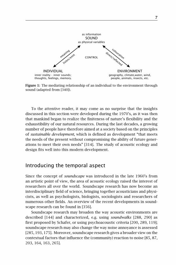
7
geography, climate,water, wind,people, animals, insects, etc.
ENVIRONMENTinner reality – inner sounds;thoughts, feelings, memory.
INDIVIDUAL
as physical variables
SOUNDas information
direct/reflected
colouration
liste
n/em
itm
eanin
g
CONTROL
Figure 1: The mediating relationship of an individual to the environment throughsound (adapted from [340]).
To the attentive reader, it may come as no surprise that the insights
discussed in this section were developed during the 1970’s, as it was then
that mankind began to realize the finiteness of nature’s flexibility and the
exhaustibility of our natural resources. During the last decades, a growing
number of people have therefore aimed at a society based on the principles
of sustainable development, which is defined as development “that meets
the needs of the present without compromising the ability of future gener-
ations to meet their own needs” [314]. The study of acoustic ecology and
design fits well into this modern development.
Introducing the temporal aspect
Since the concept of soundscape was introduced in the late 1960’s from
an artistic point of view, the area of acoustic ecology raised the interest of
researchers all over the world. Soundscape research has now become an
interdisciplinary field of science, bringing together acousticians and physi-
cists, as well as psychologists, biologists, sociologists and researchers of
numerous other fields. An overview of the recent developments in sound-
scape research can be found in [356].
Soundscape research may broaden the way acoustic environments are
described [144] and characterized, e.g. using soundwalks [288, 290] as
first proposed by Schafer, or using psychoacoustic criteria [200, 289, 119];
soundscape research may also change the way noise annoyance is assessed
[285, 193, 175]. Moreover, soundscape research gives a broader view on the
contextual factors that influence the (community) reaction to noise [85, 87,
203, 164, 163, 265].
8 Introduction
A number of principal components can be found in the subjective de-
scription of soundscapes (a literature study will be given in Chapter 9); a
factor related to the temporal structure often emerges, next to components
related to the loudness and the spectrum. Although it is acknowledged that
the temporal structure plays an important role in soundscape perception,
and although the temporal structure is often mentioned in relation to noise
annoyance, studies on its influence and efforts to integrate the temporal
structure into soundscape research have been rare.
The term temporal aspect refers to the structure of the sequence of
sound events (keynote sounds, signals or soundmarks) that constitute the
soundscape. From this point of view, it makes sense to study the temporal
envelope of the sound pressure in particular. In this work, we will use the
term “temporal envelope” in a rather broad sense: it may refer to the usual
definition of the time-varying physical amplitude of the sound (exponen-
tially averaged), but also e.g. to the time-varying loudness or pitch of the
sound.
Schafer often uses the analogy between soundscapes and music [280].
Rhythm and tempo are important characteristics of music, and both can
be found in all kinds of soundscapes. Environmental soundscapes show a
pattern of day and night, of summer and winter; church bells marked the
time in the hi-fi village life soundscape; syllables denote basic rhythmic
entities in speech etc. In its broadest sense, rhythm divides the whole into
parts, and since man tries to perceive patterns in all things, an appreciation
of rhythm and temporal structure is indispensable in acoustic design.
Outline of this work
The integration of the study of the temporal structure into environmental
soundscape research will be the subject of this work. The main focus will
be on the prediction and physical evaluation of this temporal structure,
but also some initiatives will be outlined to investigate its influence on
perception.
Models to simulate and predict temporal characteristics of sound are
a first step necessary to introduce the temporal aspect into acoustic de-
sign. Since road traffic is recognized as the main source of noise in urban
area, a model for the prediction of time-varying road traffic noise will be
described in Part I. Chapter 1 will cover the main methodology; Chapter 2
will demonstrate the use of this model on a case study. Since current traf-
fic noise prediction models are mainly focused on energy equivalent sound
pressure levels and model traffic as a stationary flow of vehicles with a con-
9
stant speed, it may be interesting to find ways to adjust these models for
particular time-depending phenomena which influence energy equivalent
sound pressure levels. A topic of interest is the variation in noise immis-
sion in the vicinity of intersections, caused by the typical deceleration and
acceleration profile of vehicles. In Chapter 3, a methodology for deriving
intersection corrections for these models will be outlined.
A second prerequisite for the introduction of the temporal aspect are
suitable physical indicators, able to grasp the special characteristics of a
time-varying soundscape, and which have a clear relation to human percep-
tion. This will be the subject of Part II of this work. Chapter 4 will introduce
the main concepts and will give the necessary mathematical background.
The leitmotiv will be the echo into the soundscape of the typical complex
systems that form its sound sources. Characteristics of dynamic and com-
plex systems can be found in music, but also in natural, rural and urban
soundscapes, as will be explained in Chapter 5. This finding will lead us to
propose a novel indicator in Chapter 6 for the temporal structure of envi-
ronmental soundscapes, based on the similarity with music. Finally, a new
method to assess the relationship between temporal soundscape features
and human perception will be introduced in Chapter 7.
Parts III and IV will illustrate the application of the concepts introduced
in the first two parts of this work. In Part III, an assessment methodology
for rural and quiet urban soundscapes will be proposed, and the need for a
multi-criteria assessment including the temporal aspect will be outlined. In
Part IV, methods to assess the noise effects, and in particular noise annoy-
ance, of the temporal structure of the soundscape in an at-home context
will be investigated.
Each part of this work starts with an introducing chapter, which outlines
the main concepts, followed by one or more in-depth chapters, of which
most were published in (or submitted to) international refereed journals.
It should be noted that these chapters are included in the form in which
they were previously published or submitted. Only minor changes were
made to notation, terminology and cross-references. This will explain some
redundancy which can be found in the introduction of these chapters.
Additional information
Soundscape recordings and source code can be found at the website of
the acoustics group (http://acoustweb.intec.ugent.be). Requests for other
media or additional information may be addressed to the author via e-mail

Part ITime-dependent
Noise Prediction

Chapter1
Traffic Noise Prediction
and Assessment
1.1 Background
Current traffic noise prediction is focused on energy equivalent sound pres-
sure levels, mainly because time-average levels are relatively easy to cal-
culate and predict, and because the relationship with noise annoyance is
well documented. As it was already mentioned in the introduction, sev-
eral acoustical and non-acoustical factors influence noise annoyance. As
a consequence, the variance in noise annoyance is predicted by energy
equivalent sound pressure levels only in a limited way. In view of other
(health) effects of noise, such as sleep disturbance, the use of the energy
equivalent sound pressure level as the main indicator is even more de-
bated (see e.g. [107, 125]). For example, intermittent noise causes signifi-
cantly more sleep disturbance than non-fluctuating noise at the same time-
average level [244].
Next to this, there exists a growing tendency to assess our sonic environ-
ment in a more positive way, reflected in the current advances in sound-
scape research [356]. Since the temporal aspect plays an important role
in soundscape perception, it is an essential factor in environmental sound-
scape design. Obviously, there is a need to predict and assess the temporal
characteristics of soundscapes in a more detailed way.
In this Part, we will outline a model for the prediction of time-varying
road traffic noise. The methodology used in environmental impact assess-
ment — and particularly in environmental noise assessment (aen) — is of-
ten unraveled into the steps of the dpsir framework [294], a causal frame-
work for describing the interactions between society and the environment.

14 Traffic Noise Prediction and Assessment
This framework was defined by the European Environment Agency, and
has since been widely adopted. In essence, the dpsir framework consists
of several layers, each of which gathers information represented by indi-
cators, either measured or computed, on phenomena that are regarded as
typical for and/or critical to environmental quality. A schematic view is
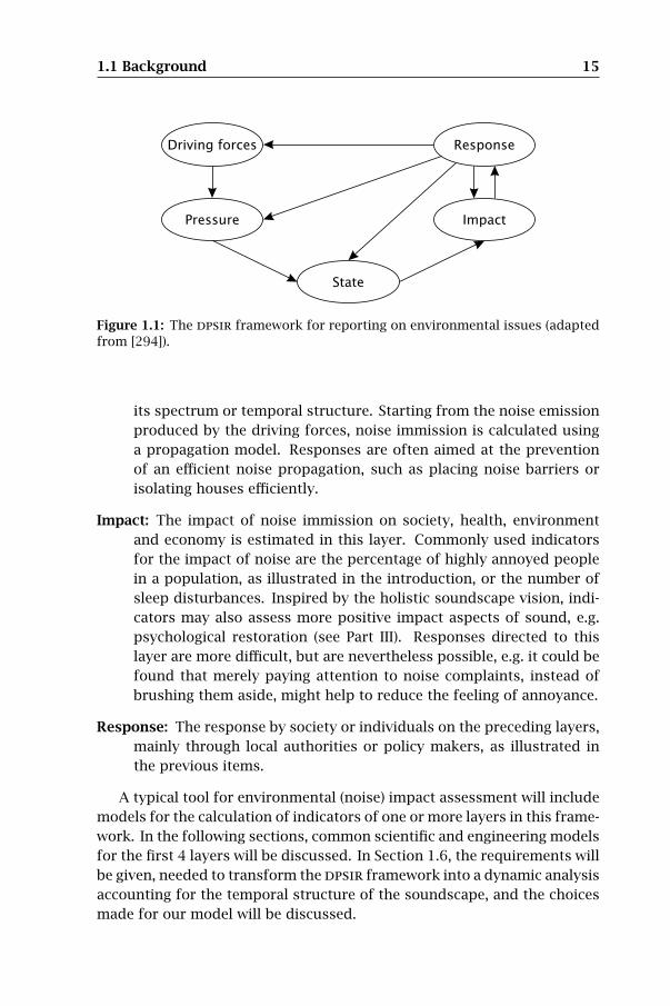
given in Figure 1.1.
An analysis in terms of the dpsir framework starts with the underly-
ing causes or driving forces (d), interwoven with socio-economic activities
such as production, consumption and transport. These driving forces ex-
ert pressure (p) on the environment, which is indicated by environmental
usage and emissions. This pressure will modify the state (s) of the envi-
ronment (air, water, soil, ecosystems…). The fourth link will evaluate the
positive or negative impact (i) of these effects on nature, health, society
and economy. Finally, controlling this impact requires response (r) on all
levels, which may come from natural systems through self-regulation, or
from environmental policy makers. When applied to environmental noise
assessment, the dpsir framework takes the following form:
Driving forces: This embraces the demand for mobility, freight transpor-
tation, recreation, construction etc. In this Part, the focus will be on
the most important driving force in urban environment: road traffic.
Corresponding indicators are the various traffic metrics, measured or
simulated by the use of traffic simulation models. Responses directed
to this layer are often structural solutions, such as the adoption of
different town planning strategies or the rerouting of traffic by the
use of traffic management infrastructure.
Pressure: This is the noise emission produced by the driving forces. Each
type of source has its own typical noise, characterized by its sound
power, frequency content, duration etc. A commonly used indicator
for this layer is the average traffic noise source power level emitted
per segment of road, LW,s . Examples of responses directed to this
layer are lowering the maximum allowed noise emission level of ve-
hicles, the introduction of quiet road surfaces, or restricting the way
vehicles are used, e.g. by enforcing speed limits.
State: In this layer, the state of the environment is reported, represented by
the noise immission, which focuses on the noise exposure at a certain
location, linked to a human observer. Typical indicators are the aver-
age A-weighted sound exposure level LAeq and derived measures such
as Ldn or Lden, and percentile noise levels such as LA50 or LA95. Indi-
cators may however also assess other dimensions of sound, such as
1.1 Background 15
Response
Impact
State
Pressure
Driving forces
Figure 1.1: The dpsir framework for reporting on environmental issues (adaptedfrom [294]).
its spectrum or temporal structure. Starting from the noise emission
produced by the driving forces, noise immission is calculated using
a propagation model. Responses are often aimed at the prevention
of an efficient noise propagation, such as placing noise barriers or
isolating houses efficiently.
Impact: The impact of noise immission on society, health, environment
and economy is estimated in this layer. Commonly used indicators
for the impact of noise are the percentage of highly annoyed people
in a population, as illustrated in the introduction, or the number of
sleep disturbances. Inspired by the holistic soundscape vision, indi-
cators may also assess more positive impact aspects of sound, e.g.
psychological restoration (see Part III). Responses directed to this
layer are more difficult, but are nevertheless possible, e.g. it could be
found that merely paying attention to noise complaints, instead of
brushing them aside, might help to reduce the feeling of annoyance.
Response: The response by society or individuals on the preceding layers,
mainly through local authorities or policy makers, as illustrated in
the previous items.
A typical tool for environmental (noise) impact assessment will include
models for the calculation of indicators of one or more layers in this frame-
work. In the following sections, common scientific and engineering models
for the first 4 layers will be discussed. In Section 1.6, the requirements will
be given, needed to transform the dpsir framework into a dynamic analysis
accounting for the temporal structure of the soundscape, and the choices
made for our model will be discussed.

16 Traffic Noise Prediction and Assessment
1.2 Traffic modeling
The interest in the study of traffic dynamics is surprisingly old. During the
1930’s, road traffic was studied by Greenshields [124], and already in the
1950’s, there was a considerable amount of scientific research concerning
the subject (see [139] for a historical review). During the last 50 years,
the traffic situation has become a lot more dramatic. The ever increasing
amount of scientific research spent on traffic dynamics has led to a mul-
titude of traffic models, each with its own distinct characteristics. What
they do have in common is that they were originally developed to study
traffic logistics problems and to predict travel times, congestion and traffic
jams. As such, there exists a gap between what traffic models are able to
provide, and what noise emission models (Section 1.3) require to operate
correctly [253].
This section will provide a brief overview of the most important types
of traffic models; where necessary, their strengths and weaknesses for ap-
plication with noise emission models will be discussed. One has to bear
in mind the difference between transportation planning models and traf-
fic flow models [202]. The former deal with the decisions made by travel-
ers (households, industrial transportation…), which lead to travel demands
and traffic. The latter explicitly describe the physical propagation of traffic
flows in a road network, on a lower level. Within the context of this work,
traffic flow models are of main interest; the travel demands are assumed to
be given. However, practical application of traffic models requires knowl-
edge of both, since often the difference is blurred in software implementa-
tions.
1.2.1 Transportation planning models
The main idea behind these models is that the transportation needs of trav-
elers are motivated by social, economical and cultural activities, which are
spatially separated (e.g. living vs. working area). Models to map these sep-
arations are called land use models, which are used to calculate the derived
transportation intentions or activity patterns, based on the socio-economic
behaviour of individual people [202]. The transportation planning model
will then link these activity patterns to the transportation infrastructure.
Two approaches exist: trip-based and activity-based.
The trip-based approach is the oldest and most widely used methodol-
ogy (for a historical review, see [47]). Central to this approach is the notion
of aggregated traffic demand. A trip-based model generally consists of
4 steps:
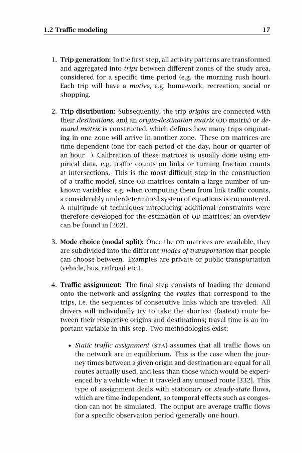
1.2 Traffic modeling 17
1. Trip generation: In the first step, all activity patterns are transformed
and aggregated into trips between different zones of the study area,
considered for a specific time period (e.g. the morning rush hour).
Each trip will have a motive, e.g. home-work, recreation, social or
shopping.
2. Trip distribution: Subsequently, the trip origins are connected with
their destinations, and an origin-destination matrix (od matrix) or de-
mand matrix is constructed, which defines how many trips originat-
ing in one zone will arrive in another zone. These od matrices are
time dependent (one for each period of the day, hour or quarter of
an hour…). Calibration of these matrices is usually done using em-
pirical data, e.g. traffic counts on links or turning fraction counts
at intersections. This is the most difficult step in the construction
of a traffic model, since od matrices contain a large number of un-
known variables: e.g. when computing them from link traffic counts,
a considerably underdetermined system of equations is encountered.
A multitude of techniques introducing additional constraints were
therefore developed for the estimation of od matrices; an overview
can be found in [202].
3. Mode choice (modal split): Once the od matrices are available, they
are subdivided into the different modes of transportation that people
can choose between. Examples are private or public transportation
(vehicle, bus, railroad etc.).
4. Traffic assignment: The final step consists of loading the demand
onto the network and assigning the routes that correspond to the
trips, i.e. the sequences of consecutive links which are traveled. All
drivers will individually try to take the shortest (fastest) route be-
tween their respective origins and destinations; travel time is an im-
portant variable in this step. Two methodologies exist:
• Static traffic assignment (sta) assumes that all traffic flows on
the network are in equilibrium. This is the case when the jour-
ney times between a given origin and destination are equal for all
routes actually used, and less than those which would be experi-
enced by a vehicle when it traveled any unused route [332]. This
type of assignment deals with stationary or steady-state flows,
which are time-independent, so temporal effects such as conges-
tion can not be simulated. The output are average traffic flows
for a specific observation period (generally one hour).
18 Traffic Noise Prediction and Assessment
• Dynamic traffic assignement (dta) resembles sta, but instead
of allocating routes once, they are dynamically reallocated, tak-
ing into account time-dependent delays, which results in time-
varying flows on links [113]. The temporal resolution is only
limited by the temporal resolution of the traffic flow model used.
Two submodels are used for this purpose. The route choice
model is essentially the same as in the case of sta, extended
with a spreading of the departure time, as a sta approach as-
sumes that all traffic is simultaneously assigned to the network.
The dynamic network loading model balances the traffic load on
the network and generates the dynamic behaviour.
While trip-based transportation planning models were refined exten-
sively during the past decades and are widely used, some problems are
difficult to solve with this aggregate approach, e.g. shops that remain open
late, flexible working hours for employees or members of a household par-
ticipating in joint activities [202]. Activity-based models [4, 94] therefore
consider individual activity patterns as the basic unit for transportation
planning. The interaction between members of a household and the rela-
tion to their induced travel behaviour is studied.
In contrast to trip-based models, there is no explicit framework encap-
sulating the activity-based approach. however, certain building blocks can
be recognized in most models [202], such as submodels for the generation
of activities, for household choices and for time scheduling. Activity-based
models are usually implemented as a multi-agent system, in which the in-
dividual households are represented as agents, often combined with a mi-
croscopic traffic flow model. The activity-based approach is still a mostly
academic research field, since an extensive amount of specifically tailored
data is needed.
1.2.2 Traffic flow models
Traffic flows can be studied on different scales. On a microscopic scale,
traffic flows are composed of individual vehicle-driver units, each of which
has its own characteristics. Dynamic aspects of these flows are mainly pre-
scribed by the underlying behaviour of the drivers and vehicles. The main
vehicle related variables are the vehicle length, position, speed, accelera-
tion and headway (distance to the vehicle in front). Driver related variables
could be its reaction time, stress level, age, medical condition etc. Since the
inclusion of driver behaviour would lead to a severe increase in complexity,
these human factors are seldom taken into account, although the research
into driver behaviour is gaining momentum [202].

1.2 Traffic modeling 19
On a macroscopic scale, the main characteristics of a traffic stream are
its density (expressed in number of vehicles per km), its rate of flow Q
(expressed in number of vehicles per hour), its occupancy (the fraction of
time a location is occupied by a vehicle) and its mean speed (space- or time-
averaged). The mathematical treatment of the fundamental relationships
between different traffic flow parameters, as well as of the different traffic
flow regimes (free flow, capacity flow, congested traffic…), is the field of
traffic flow theory; we refer to [1] for a state-of-the-art report.
Traffic flow simulation models are designed to mimic the behaviour of
real life traffic flows, and are used to analyze a wide range of applications
where a mathematical treatment is infeasible due to the spatial/temporal
scale or the complexity of the traffic flow process. Traffic flow simulation
models can be categorized based on their treatment of time (operation in
continuous time, in discrete time or event-based), based on process rep-
resentation (deterministic or stochastic), based on the scale of application
(describing a single roadway, an entire network, a city etc.) or based on
their level of detail [147]. In the context of traffic noise prediction, a cate-
gorization in terms of the level of detail is the most advantageous, as this
characteristic has a large influence on the coupling with noise emission
models. Based on their level of detail, traffic flow simulation models can
be classified into the following four categories:
Macroscopic models: Traffic streams are described at an aggregated level.
Both vehicles and their interactions are described at a low level of
detail. The underlying concept is the continuity assumption, which
states that vehicle stream parameters can be treated as continuous.
In this case, the theory of fluid dynamics (Navier-Stokes equations)
can be applied to traffic streams. A famous example is the lwr
model, independently derived by Lighthill and Whitham [197] and
Richards [270], also called the kinematic wave model. The continu-
ity assumption holds true when the macroscopic spatial and tempo-
ral scales are considerably larger than the largest vehicle-associated
scales. This makes macroscopic traffic flow simulation models not
suited for time-varying traffic noise prediction.
Mesoscopic models: Traffic streams are still described at an aggregated
level. Vehicles and driver behaviour are not described individually,
but rather in more aggregated terms, e.g. using probability distribu-
tions. However, the behaviour rules are described at an individual
level, to be able to produce more complex and non-linear dynamics
such as different traffic regimes. The term “mesoscopic models” is
often used synonymous with gas-kinetic models, based on the Boltz-
20 Traffic Noise Prediction and Assessment
mann theory of gas dynamics. A famous example is the Prigogine-
Herman kinetic model [261]. Since the output of these models is still
at an aggregated level, they are also not a candidate for the use in
time-varying traffic noise prediction.
Microscopic models: Both vehicles and their interactions are described
at a high level of detail. Vehicle characteristics such as speed, ac-
celeration and headway are simulated. A classical example are car-
following models, which were already studied in the 1950’s (see e.g.
[256]) and have been refined extensively since then [48]; a partic-
ular improvement was the introduction of lane-changing rules for
multi-lane roads. Microscopic models have always been regarded as
time consuming and complex; however, since the 1990’s, new micro-
scopic models were developed based on cellular automata [339], pos-
sibly driven by the exponential growth in available computing power.
These traffic cellular automata — commonly referred to as microsim-
ulation models — are dynamic, self-driven, many particle systems,
operating far from equilibrium. For an overview of this fast evolving
research field we refer the interested reader to [56, 139, 282]. Sev-
eral computer implementations, pure scientific as well as commercial,
have been built around these models. These often incorporate car fol-
lowing and lane-changing models, as well as transportation planning
models operating at a higher level, e.g. traffic assignment models.
Most microscopic traffic simulators allow to build a road network
and often allow qualitative visualisation (Figure 1.2). An extensive
overview of most existing microsimulation models can be found in [2].
Sub-microscopic models: These models have an even greater level of de-
tail. While microscopic models consider a vehicle as the elementary
unit, sub-microscopic models also describe the vehicle’s inner work-
ings, such as engine performance, gearbox operations or steering ma-
noeuvres, and may even describe the human driver’s decision making
process [202]. Implementations are up to now only of academic inter-
est; we cite the mixic model [315] developed at tno as an example.
1.3 Noise emission modeling
In the framework of traffic noise prediction and noise mapping, the noise
emission produced by road traffic is assessed using a traffic noise emission
model. Only the level of noise emission is of interest (total or in spectral
bands), as opposed to the case of auralization [177], in which the actual
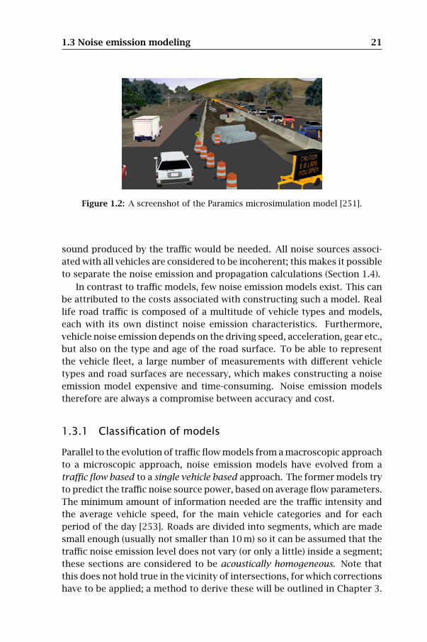
1.3 Noise emission modeling 21
Figure 1.2: A screenshot of the Paramics microsimulation model [251].
sound produced by the traffic would be needed. All noise sources associ-
ated with all vehicles are considered to be incoherent; this makes it possible
to separate the noise emission and propagation calculations (Section 1.4).
In contrast to traffic models, few noise emission models exist. This can
be attributed to the costs associated with constructing such a model. Real
life road traffic is composed of a multitude of vehicle types and models,
each with its own distinct noise emission characteristics. Furthermore,
vehicle noise emission depends on the driving speed, acceleration, gear etc.,
but also on the type and age of the road surface. To be able to represent
the vehicle fleet, a large number of measurements with different vehicle
types and road surfaces are necessary, which makes constructing a noise
emission model expensive and time-consuming. Noise emission models
therefore are always a compromise between accuracy and cost.
1.3.1 Classification of models
Parallel to the evolution of traffic flow models from a macroscopic approach
to a microscopic approach, noise emission models have evolved from a
traffic flow based to a single vehicle based approach. The former models try
to predict the traffic noise source power, based on average flow parameters.
The minimum amount of information needed are the traffic intensity and
the average vehicle speed, for the main vehicle categories and for each
period of the day [253]. Roads are divided into segments, which are made
small enough (usually not smaller than 10 m) so it can be assumed that the
traffic noise emission level does not vary (or only a little) inside a segment;
these sections are considered to be acoustically homogeneous. Note that
this does not hold true in the vicinity of intersections, for which corrections
have to be applied; a method to derive these will be outlined in Chapter 3.

22 Traffic Noise Prediction and Assessment
The main advantage of this approach is that emission coefficients can
be estimated using statistical pass-by measurements (spb) along existing
roads. Independent of the type of propagation model used, these models
only allow to calculate energy equivalent sound pressure levels (hourly or
for certain periods of the day), and derived measures such as Lden. Note
that only this is expected by the eu [93]. Examples of this approach are the
emission database [239] used in the French road traffic noise calculation
method [240], and the Dutch calculation method [272], which also provides
a correction for different road surface types and intersections.
Single vehicle based emission models treat each vehicle as a moving
noise source, consisting of a number of sub-sources, located at different
heights above the road surface. The strength of these sources may de-
pend on various vehicle related parameters, such as the vehicle category,
its speed and acceleration, as well as on road surface parameters; usually a
semi-analytical approach is used. Single vehicle based emission models can
be naturally combined with point-to-point propagation models. Another
advantage of using single vehicle based emission models is that vehicle
speed and acceleration distributions can be taken into account, if these are
provided by the traffic flow model used, as demonstrated in [253]. For time
dependent traffic noise prediction, single vehicle based emission models
are necessary. The two main models, which are the Nord 2000 model [167]
and the Harmonoise model [166], are discussed more in depth in the next
sections.
1.3.2 The Nord 2000 model
This is the first single vehicle based emission model, developed in the
framework of a major revision of the Nordic environmental noise predic-
tion model [181]. The goal of this reference model was very ambitious:
the model would provide a complete separation of tyre/road noise, en-
gine noise and aerodynamic noise; 5 vehicle categories were proposed,
some which have sub-categories; 8 main road categories were proposed;
corrections for 6 different types of driving conditions were outlined. With
each source, an iso one-third octave band emission spectrum is associated,
which depends on the vehicle type and speed.
However, this model can only be used in a somewhat crippled form,
due to insufficient measurement data. Only data (in tabular format) for the
3 main vehicle categories is available, for one type of road surface (typical
Danish surface) and one driving condition (cruising). Furthermore it is
proposed to use only a single directed noise source for each vehicle. A
major shortcoming is that only vehicles with a speed ≥ 30 km·h−1 can be
modeled, which is a consequence of the measurement method used (pass-

1.3 Noise emission modeling 23
by measurements of single vehicles [154]). Together with the fact that
acceleration corrections are not available, this model is of rather limited
use for traffic noise prediction in urban area. However, up to 2004, it was
the only single vehicle based emission model publicly available.
1.3.3 The Harmonoise model
This model was developed in the framework of the Harmonoise project [80],
partly funded by the eu, which was basically oriented at a harmonization
of environmental noise prediction models in Europe. The model is based
on extensive measurement campaigns performed at several locations in Eu-
rope, including statistical pass-by (spb) measurements and close-proximity
(cpx) measurements [155] carried out on vehicles in real traffic.
Rolling noise (combined with aerodynamic noise) and propulsion (en-
gine) noise are separately modeled; both contributions are resp. given by
the following formulas [166]:
LWR(f ) = aR(f )+ bR(f ) · log10
[v
vref
](1.1)
LWP(f ) = aP(f )+ bP(f ) ·
[v − vrefvref
](1.2)
where v is the vehicle speed (in km·h−1) and vref = 70 km·h−1. These
formulas are valid under the reference condition of a vehicle cruising at
constant speed on the (virtual) Harmonoise reference road surface, with an
air temperature of 20 ◦C. Coefficients aX(f ) and bX(f ) are given in one-
third octave bands, with center frequency f ranging from 25 Hz to 10 kHz,
and for 3 main vehicle categories: passenger cars, medium heavy and heavy
vehicles. A further subdivision of the heavy vehicle class is made using a
correction onaR(f ) for the number of axles. 80 % of the rolling noise sound
power is assigned to a point source at a height of 0.01 m above the road
surface, and 20 % is assigned to a point source at 0.30 m (passenger cars)
or 0.75 m (heavy vehicles) above the road surface; the opposite is true for
the propulsion noise.
Furthermore, corrections on the rolling noise (Eq. 1.1) are given for dif-
ferent air temperatures and road surface types, for surface age and wet-
ness, and for the use of studded tyres. Corrections on the propulsion noise
(Eq. 1.2) are given for accelerating/decelerating vehicles; corrections for dif-
ferent driving conditions are therefore not necessary. To take into account
the screening of the car body and the horn effect of tyre/road noise, each
point source also is assigned a specific frequency dependent horizontal
and vertical directivity.
24 Traffic Noise Prediction and Assessment
1.4 Sound propagation modeling
To obtain the noise immission, which describes the state of the environ-
ment, the propagation of sound from its source through the environment
has to be simulated. A large number of propagation models is available,
but not all are suited for the use in environmental noise assessment; an
overview of the most widely used models can be found in [78]. In order
to minimize the computational cost, most classic engineering traffic noise
prediction models use a simplified propagation model, in which only the
direct propagation path is considered, in some cases extended with a reflec-
tion correction. Although these models are a good compromise for large
scale noise mapping purposes, reflection and diffraction of noise has to be
taken into account when one considers more detailed urban areas. Gener-
ally, two categories of models suited for this purpose exist: discretization
and geometric models.
Discretization models divide the environment into small elements; the
acoustic wave equations are discretized and usually made linear. Exam-
ples are the radiosity method, which has been found effective for simulat-
ing diffuse reflection of sound in street canyons and town squares [170],
the diffusion method [254], the boundary element method (bem) [291], the
parabolic equation (pe) method [277] and the finite-difference time-domain
(fdtd) method, which may be applied to a moving atmosphere [320]. A ma-
jor drawback of discretization models is that for non-trivial environments,
such as large urban areas with buildings, a massive amount of elementary
cells is needed to be able to model the broad frequency range (up to 10 kHz)
needed for noise mapping.
Geometric models (also called ray-based models) are based on the as-
sumption that sound waves can be described as rays. Once a valid path
for a ray is found, the computation time is no longer dependent on the
frequency of interest, which overcomes the main problem of discretiza-
tion methods. The challenge is now to develop efficient algorithms to find
all possible paths between each source and each immission point, taking
into account the possibility of rays making (multiple) reflections against
buildings, or (multiple) diffractions around edges. The typical spatial co-
herence of rays can be exploited by grouping them into cones, prisms or
general polygonal beams. A particular method is object precise polygonal
beam tracing [138, 114], in which the beams preserve the geometry of the
environment.
In the framework of an earlier Ph. D. work at our research group, an ef-
ficient implementation of an object precise polygonal beam tracing model
was carried out. An in depth discussion of this model can be found in [78];
1.5 State indicators for impact analysis 25
a concise overview will be given in Section 2.2.3. The model originally was
intended for use in urban area, and as such, taking multiple reflections
and diffractions in the horizontal plane into account is its main strength.
Vertically, only a single path over the rooftops of the buildings is mod-
eled; this approach is often referred to as a 2.5 dimensional method. The
model was later generalized to full 3D [74]. This extended model makes it
possible to simulate noise propagation in non-trivial geometries, and over
undulating terrain such as an alpine area; however with the drawback of
a substantially larger need for computing power. The attenuation of rays
when propagating, reflecting and diffracting, is calculated based on the
iso 9613 standard [157] and the Nord 2000 engineering model [258] for
outdoor sound propagation.
It has to be noted that in noise mapping, it is usually assumed that dif-
ferent noise sources, originating from different parts of a vehicle, as well as
originating from different vehicles, are incoherent. Under this assumption,
all noise sources can be processed separately by the propagation model,
without taking the phase into account. Regarding the scale of interest in
this work (small urban areas, single intersections), it is advisable that the
claim of incoherence is checked. In [158] it is found that interference ef-
fects only have a significant influence in narrow street canyons (width less
than 10 m) with perfectly flat walls, and at low frequencies.Structured walls,
which are common in built-up urban area, lead to a diffusion of sound en-
ergy and smooth out the effect of interference. Additionally, atmospheric
turbulence and wind produced by moving vehicles may further decrease
the possible influence of interference effects.
1.5 State indicators for impact analysis
In environmental noise impact assessment, a link is drawn between phys-
ical noise immission indicators and human perception. When chosing ap-
propriate indicators, the field of application (noise annoyance, speech in-
terference, sleep disturbance…) plays an important role. Traditionally, a
good indicator should fulfill the following requirements [335]:
1. Validity: There should be a (scientifically proven) relation between
the indicator and the noise effect considered;
2. Practical applicability: It should be relatively easy to measure the
indicator, or to compute it based on available data;
3. Transparency: The indicator should be easy to explain and intuitive;

26 Traffic Noise Prediction and Assessment
4. Enforceability: When limit values are proposed, it should be possible
to easily find out when these are exceeded;
5. Consistency: New indicators should only deviate strongly from cur-
rent practice if it can be demonstrated that they have significant ad-
vantages over existing ones.
1.5.1 Classical indicators
Traditional noise immission indices are aimed at providing an estimate for
the perceived loudness of a period of noise or a noise event. Generally, they
can be categorized based on several criteria [335]:
Frequency aspects: The frequency content is often reduced to 1 number.
Since the sensitivity of the human auditory system is dependent on
the frequency, a frequency weighting is applied. The A-weighting
filter is most often used [64], which provides a rough approximation
of the relative sensitivity of the human auditory system at a total level
of about 40 dB. Other possibilities are B- or C-weighting, the perceived
noise level pnl, or the use of a more elaborate psychacoustic model
for loudness (e.g. Zwicker loudness [352]). It has to be noted that A-
weighting underestimates low frequency noise, which has been linked
to noise effects of some severity [16].
Noise period description: Three commonly used methods exist to evalu-
ate the level of a noise event or period. The first method consists of
calculating the energetic mean or sum of the sound pressure (LAeq or
ASEL). The second method consists of calculating a percentile value
LAx, which represents the level that has been exceeded during x % of
the time. Often used are LA10 (peak level), LA50 or LA95 (background
level). Percentile levels have the disadvantage that they are not ad-
ditive, which complicates their use in noise prediction models. The
third method only considers the maximum level of the period (LAmax),
which can be seen as a special case of percentile value (LA0). This
method ignores the fact that an event can have a long or a short du-
ration, and presumably a longer event is more likely to cause effects
than a very short event.
Long-term mean: When average levels are considered, these may be fur-
ther aggregated to longer timespans in different ways. An often used
indicator is LAeq,24h, which represents a 24-hour average value. Of-
ten, different periods of a day are given different weights, to reflect
the human sensitivity to environmental noise during these specific

1.5 State indicators for impact analysis 27
periods. Examples are Ldn (day and night) and Lden (day, evening and
night) [93].
As already stated in the introduction, noise annoyance is seen as the
most important effect of noise. The traditional method for noise annoy-
ance assessment consists of using exposure-effect relationships [217], in
which the prevalent state indicator is LAeq and its derived measures Ldn
and Lden [93, 334]). Percentile levels are used in some particular cases, e.g.
LA10 in the British legislation [65]. In an attempt to incorporate the an-
noyance caused by fluctuating noise, several more experimental indicators
have been proposed, such as the traffic noise index tni or the noise pol-
lution level LNP, which both are a linear combination of several percentile
levels; however, their use has never been widespread.
1.5.2 Modern approaches to noise annoyance
Contextual variables which influence noise annoyance, such as noise sen-
sitivity, may be included in traditional methods by introducing a shift in
Ldn [162, 218, 219, 215]. However, this approach has several fundamental
shortcomings [192, 193]: only single sources are assessed, interactions be-
tween the observer and its environment are neglected, and noise annoyance
is derived from aggregated data, which can not be transferred to specific
situations or contexts (see also Section 10.1).
Recent efforts have been made at our research group to introduce soft
computing methods into noise impact assessment [44, 45, 46, 324], as a
way to account for the inherent vagueness in concepts such as annoyance,
as well as for the contextual and personal factors that play a role in the per-
ception of noise. Two strategies can be discerned: fuzzy rule base methods
(frb) and fuzzy neural networks (funn). Instead of averaging out the un-
certainty related to contextual and personal factors, as is done in the tradi-
tional methods, it is explicitly taken into account using fuzzy mathematics.
Fuzzy rule bases explicitly use linguistic terms instead of crisp values, and
express the knowledge as if-then rules in natural language. Fuzzy neu-
ral networks approximate the knowledge using a structure resembling a
neural network having learning capabilities.
Traditional approaches all have in common that they model the aver-
age response of a population, thereby not explaining how noise annoy-
ance emerges. A relatively new method consists of building a causal model
for the emergence of noise annoyance at the level of the individual per-
son [78, 79]. The key hypothesis of this model is that noise has to be
noticed before it can become annoying [103, 281]. Personal factors that
modify noise annoyance are modeled on an individual basis. The distri-

28 Traffic Noise Prediction and Assessment
bution of annoyance observed in experiments or surveys is predicted by
simulating a large number of persons. A detailed description of this model
as well as experimental results can be found in [78].
1.5.3 Towards a more positive approach
Putting the focus on noise levels and annoyance is a negative approach, as
it was already mentioned in the introduction. To assess the soundscape
in a more holistic way, more than one indicator will be needed, since the
soundscape is perceived as having multiple (orthogonal) dimensions: loud-
ness, spectral content, temporal structure etc. (this will be more elaborated
in Part III). In Part II, we will introduce a novel indicator which grasps the
special temporal characteristics of a time-varying soundscape, and which
may be easily calculated using the model described in this chapter.
1.6 Time-dependent noise prediction
Based on the overview given in the previous sections, the construction of
the time dependent traffic noise prediction model used in this work can
now be sketched as follows:
Traffic model: Traffic should be modeled at least on a microscopic level.
The commercial microsimulation software package Paramics [251]
was chosen, since the development of an own model would be un-
feasible. Paramics incorporates a dynamic traffic assignment model,
since vehicles do not carry routing information for more than two
links ahead, other than knowing which destination they are headed
for. The spreading of the departure time is random; therefore, to
achieve a realistic traffic distribution consisting of smaller and larger
groups of vehicles, one has to model an area larger than the area
under study. The dense network of intersections and traffic man-
agement devices such as traffic lights in an urban area may however
make this more easier to achieve, as will be shown in Chapter 4. An
example of the construction of a simulation network in Paramics will
be given in Section 2.3.1.
Emission model: The Nord 2000 model was used for the simulations dis-
cussed in Chapter 2 and 6. When it became public available, the Har-
monoise model was implemented, and all further simulations in this
work were carried out with this model (Chapter 3 and 9). The Har-
monoise model has the main advantage that the deceleration and ac-
celeration at intersections is more accurately modeled. The emission

1.6 Time-dependent noise prediction 29
Table 1.1: Comparison between the classical approach for traffic noise predictionand our prediction model for time-varying road traffic noise, according to the dpsir
framework.
Implementation Classical approach Dynamic model
D traffic model macroscopic microscopic (Paramics)
P emission model traffic flow based single vehicle based(Nord 2000, Harmonoise)
S propagation model direct path, efficient object preciseray-based polygonal beamtrace model
indicators LAeq , Ldn, Lden, LAx also temporal structure(see Part II)
model is implemented as a plugin for the Paramics simulation pack-
age.
Propagation model: The object precise polygonal beam tracing model de-
veloped at our research group was chosen, which gives a suitable
balance between calculation time and accuracy. Restraining the cal-
culation time is essential when time-varying noise maps have to be
calculated, needed for some of the state indicators focused on. There-
fore, the path generation algorithm, taking into account reflections
and diffractions, has been implemented with performance in mind.
State indicators for impact assessment: Although this model is able to
calculate traditional average levels, the main purpose of this model
will be to calculate percentile levels, as well as indicators which de-
scribe the temporal structure (introduced in Part II).
Table 1.1 shows a comparison with the classical approach. For large scale
noise mapping projects, the microsimulation submodel forms the largest
bottleneck, since coding and validating a network requires intensive and
time-consuming manual editing. Constructing a micromodel is thus only
feasible for small area networks (see e.g. Chapter 2), or canonical situations
(see e.g. Chapter 3). Since the beamtrace propagation model is developed
with performance in mind, computation speed and memory do not pose in-
surmountable problems on the applicability of the noise prediction model
in built-up small area networks.
Vagueness and imperfections are introduced in all stages of the noise
prediction model, because of model imperfections and a lack of or vague-
ness in input data. These uncertainties then propagate to the subsequent
links in the chain of submodels. Typical uncertainties in the input data

30 Traffic Noise Prediction and Assessment
are related to the traffic flow intensity, the vehicle speed distribution, the
fraction of heavy vehicles, the ground surface type, the building geometry
etc. Typical model imperfections are: not taking into account the noise
from local businesses, simplifying the influence of atmospheric conditions
and the ground effect in sound propagation, neglecting the effect of diffuse
reflections etc. We require that the model is able to accurately predict the
temporal structure of the soundscape in small area networks and canonical
situations.
The sensitivity of traffic noise prediction models to variations in the in-
put data has been investigated thoroughly in the imagine project [321]. To
account for the above mentioned aspects of uncertainty, the chosen prop-
agation model applies the technique of extended numbers, which replaces
regular numbers by a possibility or probability distribution. Uncertainties
in input data and model are combined to build fuzzy noise maps, which
quantify the uncertainty of the noise mapping process. We refer to [78]
for a more in depth discussion of uncertainty in noise mapping. In this
work, it is assumed that model and input uncertainties only have a small
effect on the temporal structure of the simulated noise, compared to their
possible influence on simulated noise levels.
As far as it’s known by the author, Oshino et al. [247] were the first
to make a coupling between a simple microsimulation model and a noise
emission model for individual vehicles. In more recent models, a propaga-
tion model is added. We mention the models developed at the University
of Oviedo [252, 351] and at the University of Leeds [198, 123, 122], which
are all capable of assessing (statistical) traffic noise levels in complex ur-
ban built-up environments. In our model, the emphasis is on assessing the
temporal aspects of (urban) soundscapes, which makes it rather unique.

Chapter2
The Influence of
Traffic Flow Dynamics
on Urban Soundscapes
B. De Coensel, T. De Muer,
I. Yperman and D. Botteldooren
Published in Applied Acoustics 66(2):175–194, 2005.
« « «
This chapter outlines the construction of a traffic noise prediction
model, which is able to take into account the temporal structure of
traffic noise, using the building blocks discussed in the previous chap-
ter. The use of this model is demonstrated with a case study. This
work was carried out in the framework of the mobilee project, funded
by the Belgian federal office for scientific affairs [152]. Results of this
research were presented at the 18th International Congress on Acous-
tics [39], and also a lay language version of this chapter was published
in Geluid [71].
2.1 Introduction
To guarantee mobility while minimizing its negative impact on man and
environment, is one of the main challenges for sustainable development
of our society. Although the interest in the study of traffic dynamics is
more than 50 years old [124] and in spite of many efforts to cope with
the ever growing mobility demand, in the last decades the traffic situation
has deteriorated a lot. The time that drivers spend standing in traffic jams

32 Traffic Flow Dynamics & Urban Soundscapes
amounts to several days each year; vehicle emissions have reached or even
exceeded a level comparable to those by industrial production and those
by private households.
An important consequence, particularly but not only in urban environ-
ment, is disturbance by noise. The assessment of the impact of mobility on
the urban sound climate and the quality of life, is mostly based on the cal-
culation of noise maps, using a set of standard calculation schemes for the
evaluation of the contribution of different sources. This has already been
extended to mapping the expected percentage of highly annoyed people
based on exposure–effect relationships [217]; there have even been initia-
tives to produce an integrated presentation of different environmental and
quality of life maps [35, 196].
However, today mainstream methods are mostly based on the mea-
surement and prediction of time-averaged A-weighted levels and derived
measures such as Ldn or Lden, which account for the different response
of people to noise during the evening (+5 dB(A) correction) and the night
(+10 dB(A)). Traffic is hereby modeled as a steady sound source flow. There
is a consensus that road traffic noise causes annoyance, but some stud-
ies have detected unexplained peaks of annoyance in quieter places, or
a plateau in the relation between annoyance and noise at high noise lev-
els (an overview can be found in [274]). The time pattern of the noise
of vehicles passing by may explain these anomalies. In [325], a principal
components analysis revealed three factors describing at best variations in
auditory judgment on various urban situations, one of which was strongly
correlated with the time variations of the noise. One way to modify the
dynamics of passby sound, is to concentrate on the sound quality of indi-
vidual vehicles. The sven project [183, 182, 295], for example, is looking at
a number of aspects of vehicle noise, developing methods for the objective
and subjective assessment of traffic noise quality. However, recent studies
have shown that there are also clear differences in longer-term dynamics
between different urban settings, caused by the alternation of passby noise
and background noise [70, 187].
An important tool to change traffic dynamics, and as a consequence to
change traffic noise dynamics, is traffic flow management. In the last few
years, there has been a considerable amount of effort spent on the study of
the impact of traffic light timing [179, 206], road bumps [276] and round-
abouts [311, 12] on overall noise immission levels. These studies were of
theoretical as well as of experimental nature. The need for traffic noise pre-
diction models which are able to represent interrupted and complex flow
is stressed in [300, 189].
The introduction of the time component in traffic noise prediction poses
an additional problem: what are suitable indicators? In an attempt to as-

2.2 Methodology 33
sess the annoyance caused by fluctuating noise, several descriptors have
been proposed [64], such as LA5 − LA95, N5 − N95 or LA10 − LA90. The
traffic noise index tni = 4(L10 − L90) + L90 − 30 proposed in [126] and the
noise pollution level LNP = Leq + kσ (where k is a constant and σ is the
standard deviation of the sound level) introduced in [275] are encountered
occasionally. These indicators all give an idea about the size of the fluctu-
ations from the average background noise.
However, almost exclusively only the negative aspects of the urban
sound climate are nowadays taken into account (annoyance, stress, heart
diseases, etc.), while the positive axis in the analysis of soundscapes is
seldom considered. Sometimes, it is not desirable to simply make the envi-
ronment quieter, because some urban areas ask for a matching sound, e.g.
the sound of birds in a city park or the hum of a market place [203]. From
the soundscape point of view, it looks appealing to evaluate the patterns
in time variations also. A way to do this is to calculate the power spectrum
of sound amplitude fluctuations. This was first done for music already in
the late 1970’s [328, 329], and has recently been adopted to environmental
soundscape research [69].
This paper will present a tool for dynamic traffic noise prediction. The
starting point will be the gis-based microsimulation of the traffic in an
urban neighbourhood or part of a town. Compared to the earlier work [179,
206, 276, 311, 12] that concentrated on one intersection or one street, this
has the advantage that a much more realistic traffic dynamics situation can
be created, and that sources at a greater distance also can contribute. This
microsimulation model will be coupled with a vehicle emission model and
a state of the art propagation model based on acoustic beamtrace methods,
which takes into account multiple reflections and diffractions. This way,
the soundfield at the quiet sides of buildings or in urban quiet areas can be
simulated accurately. The result will be a time series of immission values
at different observer points. These will allow to draw maps of LAeq and
statistical levels LA5, LA50, LA95 etc., but also to make maps of dynamics
descriptors based on the power spectrum of noise amplitude fluctuations.
The proposed model will be compared to measurements in Section 2.3 and
it will be illustrated how the model can be used in Section 2.4.
2.2 Methodology
2.2.1 Traffic modeling
Since the 1950’s, there is a clear evolution in the modeling of road traf-
fic [139]. The early models were based on a fluid-dynamic model for kine-

34 Traffic Flow Dynamics & Urban Soundscapes
matic waves [197], which made it possible to simulate the propagation of
density jumps in traffic; later microscopic follow-the-leader models [54]
and gas-kinetic, or so called Boltzmann-like models [261] were introduced.
In the last decade, discrete cellular automata models of vehicle traffic [61,
229], shortly called micromodels, have become very popular, mainly be-
cause of the large computing power that has become available.
In these micromodels each vehicle, represented by a particle, is simu-
lated individually. The nature of the interactions between these particles
is determined by the way vehicles influence each others movement. This
way, traffic is simulated not as a steady flow, but as a system of interacting
particles, far beyond equilibrium. The vehicle positions, speeds, velocities
and accelerations as well as the simulated time are discretized.
The traffic noise prediction model that is developed uses Paramics [251],
a commercially available microsimulation package. The basic building
blocks of Paramics road networks are nodes, corresponding to junctions,
and links, which can be subdivided into several lanes. These can be coded
starting from an overlay photograph. Different links and nodes can be
grouped into zones, each representing a certain activity, like residential
areas, industrial zones, parking lots, etc. During simulation, vehicles are
created at random, are given an origin and destination zone pair, and are
loaded onto the network on a link inside its origin zone. After reaching
their destination zone they are cleared from the network. The demands be-
tween different zones are described by a so called origin-destination matrix
(od matrix). These od matrices can be vehicle type specific to represent
the actual vehicle fleet properties; they can also vary in time. Customiza-
tion of the available vehicle types makes it possible to simulate cars, light
and heavy goods vehicles, coaches, minibusses and busses. When seperate
links and nodes are used, it is also possible to simulate the movement of
trams and trains.
2.2.2 Vehicle noise emission model
Paramics allows users to write plugins, consisting of a dynamic link library
bundling a set of callbacks, each called at defined points in the simulation.
This makes it possible to extend and refine the microsimulation model.
For our traffic noise prediction model a vehicle noise emission plugin was
written. First of all, a viewport is set, which consists of a polygonal part of
the network around the observer(s). Only vehicles inside this viewport will
be taken into account. At each timestep, positional data of each vehicle
inside the viewport is gathered, together with vehicle type, age, speed, ac-
celeration, traveling direction and additional info about the link the vehicle
is traveling on (e.g. the road surface type, the link gradient, etc.).

2.2 Methodology 35
With each vehicle, one or more sources are associated, each consisting
of an iso octave band spectrum with center frequencies from 63 Hz to
8 kHz. Emission spectra are then calculated from an external database, and
can be a function of the vehicle and link variables given in the previous
paragraph. Currently the Nord 2000 vehicle noise emission database is
used [167]. In this calculation scheme, a single directional source spectrum
is associated with each vehicle. The source is located at the right-hand side
of the vehicle at a height of 20 cm. Emission values are only function of
vehicle type and speed (in the form of tables), and only three emission
classes are used: cars (car), dual-axle heavy vehicles (dhv) and multi-axle
heavy vehicles (mhv). However, the design used makes it easy to extend
the emission model, as data becomes available. Possible extensions could
be the subdivision of vehicle emission into engine noise, tire/road noise
and exhaust noise with associated sources, or the use of corrections for
vehicle acceleration/deceleration, link gradient and road surface type.
Subsequently, the sources associated with each vehicle are mapped on
a set of emission points. Two configurations are possible:
1. A grid of emission points is placed on the part of the network in-
side the viewport. The links are segmented per lane with a user-
defined segment length; one emission point is placed in the center
of each segment. On the nodes a rectangular grid of emission points
is placed. This allows to account for wide and complex crossings and
for small roundabouts. During simulation, the vehicle sources are
mapped to the nearest emission point. When the distance between
adjacent emission points is large, it is possible that multiple sources
are mapped to the same emission point, in which case the sum of
the sound power spectra is calculated. It is also possible that vehi-
cles traveling in different directions are mapped to the same emission
point, so in this configuration the directional info cannot be taken into
account.
2. A set of emission points is constructed on the fly for each vehicle in
the network, at their exact locations. This way, directional info can be
used. However, the positions of the emission points are changed each
simulation timestep, which is a major disadvantage when it comes to
propagation calculations, as discussed below.
2.2.3 Propagation
Once a set of time-changing vehicle noise emissions are available, dynamic
noise immission at a set of observers can be calculated using a propagation
model, specially tuned for time varying sources. The model implemented
36 Traffic Flow Dynamics & Urban Soundscapes
consists of 3 steps: path generation, attenuation calculation and immission
calculation.
A beam tracing model is used to generate paths between the emission
points and the receivers. The technique used is object precise polygonal
beam tracing [138, 114]. A beam consists of a group of rays, coherent in
space (following about the same path) and bounded by the objects in the
simulation area. The model uses a 2.5D representation of the world, which
consists of a terrain model with super-positioned blocks representing the
buildings (Figure 2.1, Panel 2.5D). When looked from above, the world is
seen as a number of polygons in a plane. Standing inside the world all walls
are upright and all roofs are flat. Terrain and building data are loaded from
standard gis maps. The most important advantages of the beam tracing
approach in comparison with ray tracing is that no receivers are missed by
the infinitesimal small rays constituting the beams, and that diffraction is
modeled efficiently, which is important in high shielded regions like urban
areas.
The path generation itself is split into two parts. Firstly, a set of beams
is traced through the geometric network in 2D using the footprints of the
houses as objects (Figure 2.1, Panel 2D). The shaded areas in this figure
represent the bundles. Secondly, straight paths (as seen from above) are
constructed between each emission point and receiver within reasonable
distance, and the different diffraction and reflection points in a vertical
section are computed (Figure 2.1, Panel 0.5D).
While the beams propagate through the geometrical environment, they
reflect and diffract on boundaries, so each beam must have a local view on
the environment to efficiently perform this tracing. A convenient method to
allow this is to use a convex cell subdivision of the environment [67, 129].
Within each convex cell a beam has full visibility by definition and con-
struction. Thus, only interactions of a beam with a cell boundary have to
be described. This cell boundary can be a wall of the real world environ-
ment or a portal, which is a virtual boundary placed during the convex cell
construction. Figure 2.1, Panel Cell, shows a convex cell division where
each cell has exactly three boundaries, also called a triangulation. The
constrained Delaunay triangulation scheme is used, which preserves the
original boundaries (walls of buildings) and has among all triangulation
schemes the largest internal angle for all triangles, which is important for
the numeric stability of the implementation. Using a triangulation over a
convex polygonalization has the advantage that operations on the beams
are easy to formalize and to implement. The disadvantage is that more
beams need to be traced.

2.2 Methodology 37
Cell0.5D
2D2.5D
Figure 2.1: Beam tracing through a 2.5D environment. The emission point ( ) aswell as the receiver ( ) are shown.
Once a beam is constructed and a receiver is detected inside it, the path
between the emission point and the receiver is generated. The stack of
beams is unwound and at each real boundary the points of interest (re-
flection and diffraction points) are computed on the fly. On modern pc’s
(2 GHz) rates of 800k paths/s are achieved for the simplest configuration
down to 200k paths/s when multiple reflections and diffractions are al-
lowed, which is more than an order of magnitude faster than the actual
attenuation computation following it. Diffuse reflections are not taken
into account in the model. These can not be implemented optimally us-
ing a beamtracing technique; radiosity methods are more suited for this.
A hybrid model would ask for considerably more computing time and re-
sources.
The attenuation model is based on the iso 9613 model [157], and has
been extended with sideways diffraction according to the Nord 2000
model [258]. This model allows to take into account geometric diver-
gence, atmospheric attenuation, ground effects and meteo effects (mod-
erate downward refraction according to iso 9613).
Finally, the immission at the receiver points is calculated by multiplying
the emission with the attenuation coefficients. Two scenarios are possible,

38 Traffic Flow Dynamics & Urban Soundscapes
based on the emission point configuration (see Section 2.2.2). When exact
source positions are used as emission points, the whole propagation cal-
culation (path generation and attenuation calculation) has to be performed
at each timestep. When a fixed grid of emission points is used, the propa-
gation is done only once, and the attenuation between each emission point
and receiver pair is stored. This way, it is possible to rapidly compute im-
missions for a series of timesteps. The downside is that more memory is
needed for the calculations because there are more emission points, and
thus more paths between emission points and receivers.
For the emission points in the vicinity of receivers the source direction is
important, so the first scenario using exact vehicle positions has to be used.
Of both scenarios, this provides the most accurate results. However, the
duration of the attenuation calculation increases with the number of paths
between the emission points and the receivers, which is about proportional
to the square of the viewport radius, and also with the maximum number
of reflections and diffractions allowed. For a typical urban setting of one
receiver point and a viewport radius of 150 m, enclosing about 10 sources,
the propagation calculation has a duration of about 0.5 s, taking into ac-
count four reflections and one diffraction. When 10k receiver points are
considered, this can grow to 30 s, resulting in a 15-hour simulation time
for a 15-minute traffic simulation using a timestep of 0.5 s.
When the simulation area is large, or there is a lot of traffic, it is no
longer possible to simulate all vehicle sources using exact positions within
a reasonable amount of time. In this case a combination of both scenar-
ios has to be used, where vehicle sources at a larger distance from the
observers are mapped to an emission point grid. Paths between receivers
and sources at a greater distance are more complex, consisting of multiple
reflections and diffractions, particularly in urban environment. A direct
path is mostly not possible, so the source direction can be neglected for
these sources. In Section 2.3.3 this approach is demonstrated. The grid
used in this example has about 12k emission points; using the same prop-
agation settings as in the previous paragraph, the propagation calculation
has a duration of about 15 minutes. Subsequent immission calculations
using the attenuation coefficients stored take only about 50 ms.
When a large number of observers is placed, e.g. for the calculation
of a noise map, memory restrictions exist on the use of a grid, and it is
more feasible only to use the first scenario, but making the viewport radius
larger. This approach is illustrated in Sections 2.3.4 and 2.4.
Figure 2.2 gives an overview of the complete dynamic noise immission
model.

2.2 Methodology 39
buildingsroads
Time–varying immissions
Beamtrace propagation model
Time–varying emissions
Microsimulation model
Emissionplugin
GIS dataVehicle fleetproperties
Vehicle emissiondatabase
Figure 2.2: Methodology outline.
2.2.4 Impact analysis
Dynamic noise immission calculations result in an enormous amount of
raw data. To present these data in a condensed form in maps or tables,
suitable indicators or descriptors have to be selected. Ideally these in-
dicators reflect current knowledge on the impact on health, quality of life
(annoyance) and general appreciation of the soundscape. Unfortunately, at
least for health and annoyance effects, most recent research has focused
on long term averaged noise levels (Ldn, Lden), not explicitly taking into
account fluctuation in noise exposure level.
For traffic noise, LAeq has become the measure most commonly used.
In the past, other descriptors have also been suggested, based on the com-
mon assumption that fluctuating noise is more annoying, such as tni and
LNP, as mentioned in the introduction. The percentile level LA10 itself has
also been used to characterize traffic noise annoyance [65]. Positive sound-
scapes, in particular quiet areas, are probably not well characterized by
energy equivalent sound pressure levels. In [43] percentile noise levels,
in particular LA95 and LA50, were proven to be much better discriminators
between rural soundscapes subjectively evaluated as silent and those eval-
uated as not silent, than LAeq.
All the indices mentioned above have in common that they do not con-
sider the time pattern of the exposure. A few long noise events separated

40 Traffic Flow Dynamics & Urban Soundscapes
by long periods of relative silence may result in the same statistical levels
as a large number of short events separated by short periods of silence.
In particular for the evaluation of soundscape quality, it can be important
to distinguish between the above illustrated situations by using a suitable
indicator. It is proposed to use the spectrum of level fluctuations as an indi-
cator. To calculate this spectrum, an LAeq,1s time series of sufficiently long
duration is necessary, e.g. 15 minutes. The spectral density of this time
series is then calculated using an fft. Because fluctuations in the sound
level are considered, the corresponding frequencies are much lower, as op-
posed to the more usual spectrum of the instantaneous sound pressure.
In this spectrum, periodic events will show up as peaks. When e.g. a vehi-
cle passes by about each 10 s, one will see a peak at about 0.1 Hz in this
spectrum.
However, this spectrum has much more interesting characteristics. If
the events contributing to the soundscape result from a complex system,
then the spectrum will be linear on a log-log scale for the relevant inter-
event time scales (0.002 Hz to 0.2 Hz, or from 5 s to about 10 minutes),
according to the formula fα, with f the frequency of level fluctuations.
Self-organization of the underlying system will lead to a slope α = −1, so
called 1/f behaviour. Steeper slopes (α < −1) tend to indicate high pre-
dictability; less steep slopes (α > −1) are an indication of a chaotic process.
It was observed that 1/f spectral characteristics are quite common in ru-
ral, natural, and urban soundscapes with a mixture of activities [69] (see
Chapter 5). By drawing the link to music, where this temporal structure
was observed earlier [328, 329], it is suggested that perception of sound-
scape dynamics and the spectrum of sound level fluctuations are related
and that the slope α of the spectrum and its deviation from linearity ǫ on a
log-log scale, may be suitable soundscape descriptors [70]. To estimate α,
a linear fit of the spectrum is made in the interval from 0.002 Hz to 0.2 Hz.
Based on the above analysis, it is proposed to use LAeq, percentile noise
levels, LA5 − LA95 in particular, and the slope α of the spectrum of sound
level fluctuations as primary descriptors that summarize the dynamics of
the sound field. The latter indicator will be discussed in depth in Part II of
this work; a more detailed method to calculate α is given in Appendix A.
2.3 Case study: Gentbrugge
2.3.1 Traffic modeling and calibration
To make a validation of the model presented, a part of Gentbrugge — a sub-
urban area near Ghent, Belgium — was chosen as a study area. Figure 2.3
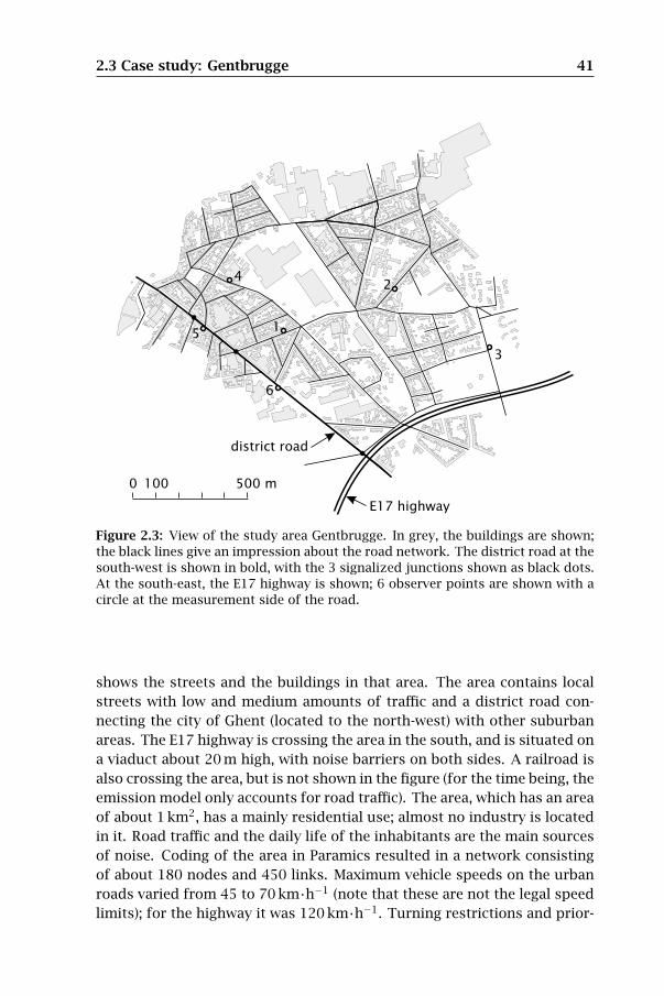
2.3 Case study: Gentbrugge 41
500 m1000
E17 highway
district road
6
5
4
3
2
1
Figure 2.3: View of the study area Gentbrugge. In grey, the buildings are shown;the black lines give an impression about the road network. The district road at thesouth-west is shown in bold, with the 3 signalized junctions shown as black dots.At the south-east, the E17 highway is shown; 6 observer points are shown with acircle at the measurement side of the road.
shows the streets and the buildings in that area. The area contains local
streets with low and medium amounts of traffic and a district road con-
necting the city of Ghent (located to the north-west) with other suburban
areas. The E17 highway is crossing the area in the south, and is situated on
a viaduct about 20 m high, with noise barriers on both sides. A railroad is
also crossing the area, but is not shown in the figure (for the time being, the
emission model only accounts for road traffic). The area, which has an area
of about 1 km2, has a mainly residential use; almost no industry is located
in it. Road traffic and the daily life of the inhabitants are the main sources
of noise. Coding of the area in Paramics resulted in a network consisting
of about 180 nodes and 450 links. Maximum vehicle speeds on the urban
roads varied from 45 to 70 km·h−1 (note that these are not the legal speed
limits); for the highway it was 120 km·h−1. Turning restrictions and prior-
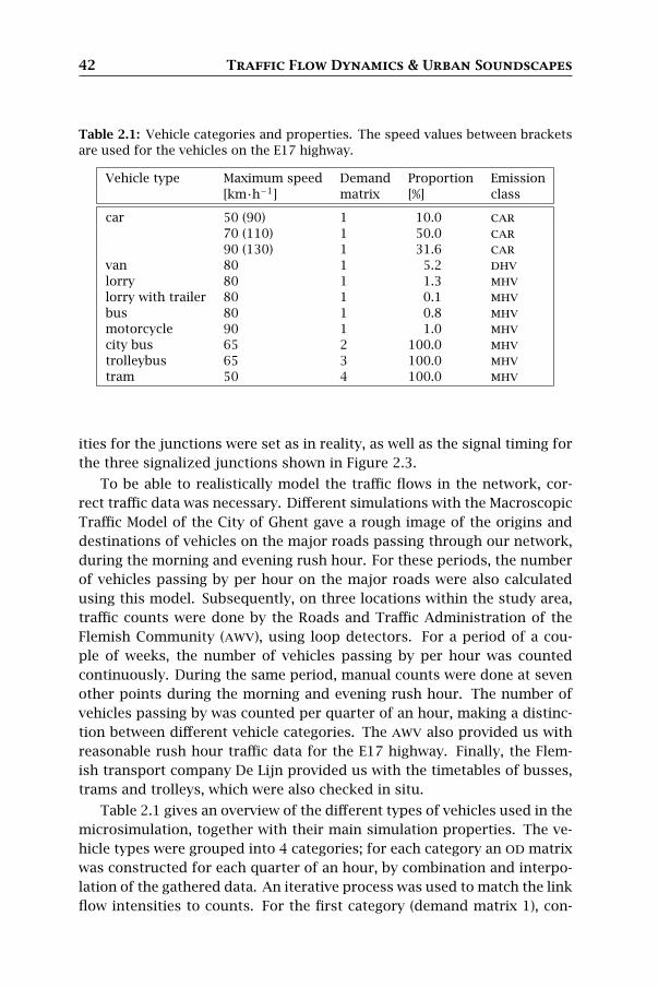
42 Traffic Flow Dynamics & Urban Soundscapes
Table 2.1: Vehicle categories and properties. The speed values between bracketsare used for the vehicles on the E17 highway.
Vehicle type Maximum speed Demand Proportion Emission[km·h−1] matrix [%] class
car 50 (90) 1 10.0 car
70 (110) 1 50.0 car
90 (130) 1 31.6 car
van 80 1 5.2 dhv
lorry 80 1 1.3 mhv
lorry with trailer 80 1 0.1 mhv
bus 80 1 0.8 mhv
motorcycle 90 1 1.0 mhv
city bus 65 2 100.0 mhv
trolleybus 65 3 100.0 mhv
tram 50 4 100.0 mhv
ities for the junctions were set as in reality, as well as the signal timing for
the three signalized junctions shown in Figure 2.3.
To be able to realistically model the traffic flows in the network, cor-
rect traffic data was necessary. Different simulations with the Macroscopic
Traffic Model of the City of Ghent gave a rough image of the origins and
destinations of vehicles on the major roads passing through our network,
during the morning and evening rush hour. For these periods, the number
of vehicles passing by per hour on the major roads were also calculated
using this model. Subsequently, on three locations within the study area,
traffic counts were done by the Roads and Traffic Administration of the
Flemish Community (awv), using loop detectors. For a period of a cou-
ple of weeks, the number of vehicles passing by per hour was counted
continuously. During the same period, manual counts were done at seven
other points during the morning and evening rush hour. The number of
vehicles passing by was counted per quarter of an hour, making a distinc-
tion between different vehicle categories. The awv also provided us with
reasonable rush hour traffic data for the E17 highway. Finally, the Flem-
ish transport company De Lijn provided us with the timetables of busses,
trams and trolleys, which were also checked in situ.
Table 2.1 gives an overview of the different types of vehicles used in the
microsimulation, together with their main simulation properties. The ve-
hicle types were grouped into 4 categories; for each category an od matrix
was constructed for each quarter of an hour, by combination and interpo-
lation of the gathered data. An iterative process was used to match the link
flow intensities to counts. For the first category (demand matrix 1), con-

2.3 Case study: Gentbrugge 43
sisting of several vehicle types, the proportions of each type are given in
Table 2.1. A number of vehicle properties, such as mean vehicle top speed,
maximum acceleration and deceleration, and a number of driver properties,
such as mean reaction time, awareness and aggressivity, were also intro-
duced in the simulation, to represent the Flemish vehicle fleet and drivers.
One has to point out that most microsimulation models tend to maximize
the vehicle driving speeds, taking into account the maximum link driving
speed and the vehicle top speed. When traffic is freely flowing, this could
result in all cars passing by at about the same speed. Therefore we divided
the car vehicle type into 3 categories with different maximum speeds, to
better represent different driving behaviour; the different percentages in
Table 2.1 for the car type are tuned to obtain the best agreement with the
actual situation.
2.3.2 Acoustic parameters
The noise immission simulation requires that some additional acoustic pa-
rameters about the vehicles and the environment are defined. Because the
Nord 2000 database only distinguishes between three emission classes, the
vehicle categories used for traffic modeling were mapped to these three cat-
egories, as shown in Table 2.1. Because no emission values for motorcycles
and trams are available up to now, these were considered to have a noise
emission comparable with the mhv class, which seemed the best compro-
mise. The information on buildings shown in Figure 2.3, to be used in the
propagation model, was loaded from gis. The external walls were assumed
to have a normalized impedance of 20, which results in a power absorption
coefficient of about 0.1 for perpendicular incidence. Because of the 2.5D
model, the buildings have a flat roof in the simulation.
For the propagation calculations, a temperature of 21 ◦C, a relative hu-
midity of 70 % and a wind direction with most probability from the south-
west were used, which are typical Flemish values for the time of year when
measurements were performed. For simulating the ground effects, the
ground was considered to be acoustically hard over the full area.
2.3.3 Comparison with immission measurements
On the 5th of June 2003, during the evening rush hour, sound measure-
ments were done at the 6 observer points shown in Figure 2.3. Using a
B&K 2260 Investigator with a B&K 4189 free field microphone mounted at
a height of 1.2 m and at a distance of 1.2 m from the edge of the road, time
series of LAeq,1s values were measured, for a period of 15 minutes. Simul-
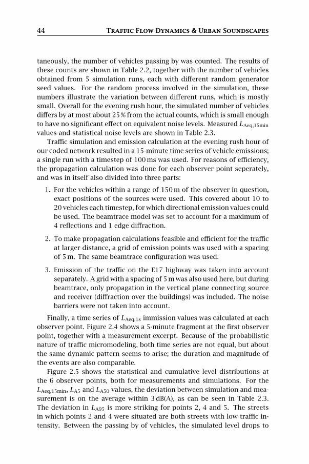
44 Traffic Flow Dynamics & Urban Soundscapes
taneously, the number of vehicles passing by was counted. The results of
these counts are shown in Table 2.2, together with the number of vehicles
obtained from 5 simulation runs, each with different random generator
seed values. For the random process involved in the simulation, these
numbers illustrate the variation between different runs, which is mostly
small. Overall for the evening rush hour, the simulated number of vehicles
differs by at most about 25 % from the actual counts, which is small enough
to have no significant effect on equivalent noise levels. Measured LAeq,15min
values and statistical noise levels are shown in Table 2.3.
Traffic simulation and emission calculation at the evening rush hour of
our coded network resulted in a 15-minute time series of vehicle emissions;
a single run with a timestep of 100 ms was used. For reasons of efficiency,
the propagation calculation was done for each observer point seperately,
and was in itself also divided into three parts:
1. For the vehicles within a range of 150 m of the observer in question,
exact positions of the sources were used. This covered about 10 to
20 vehicles each timestep, for which directional emission values could
be used. The beamtrace model was set to account for a maximum of
4 reflections and 1 edge diffraction.
2. To make propagation calculations feasible and efficient for the traffic
at larger distance, a grid of emission points was used with a spacing
of 5 m. The same beamtrace configuration was used.
3. Emission of the traffic on the E17 highway was taken into account
separately. A grid with a spacing of 5 m was also used here, but during
beamtrace, only propagation in the vertical plane connecting source
and receiver (diffraction over the buildings) was included. The noise
barriers were not taken into account.
Finally, a time series of LAeq,1s immission values was calculated at each
observer point. Figure 2.4 shows a 5-minute fragment at the first observer
point, together with a measurement excerpt. Because of the probabilistic
nature of traffic micromodeling, both time series are not equal, but about
the same dynamic pattern seems to arise; the duration and magnitude of
the events are also comparable.
Figure 2.5 shows the statistical and cumulative level distributions at
the 6 observer points, both for measurements and simulations. For the
LAeq,15min, LA5 and LA50 values, the deviation between simulation and mea-
surement is on the average within 3 dB(A), as can be seen in Table 2.3.
The deviation in LA95 is more striking for points 2, 4 and 5. The streets
in which points 2 and 4 were situated are both streets with low traffic in-
tensity. Between the passing by of vehicles, the simulated level drops to

2.3 Case study: Gentbrugge 45
Table 2.2: Vehicle counts at the observer points and results of different simulationruns. For points 1–4, vehicles were counted along the measurement side of theroad (a), and in the opposite traveling direction (b). The counts are each for aduration of 15 minutes, and include all vehicle types under consideration.
Point Measured Simulated Deviation1 2 3 4 5 Mean
1 (a) 46 39 36 46 38 38 39.4 −14.3 %1 (b) 64 72 62 77 67 77 71.0 +10.9 %2 (a) 27 36 33 35 30 33 33.4 +23.7 %2 (b) 9 7 8 10 8 9 8.4 −6.7 %3 (a) 67 79 80 78 72 84 78.6 +17.3 %3 (b) 62 57 61 59 61 64 60.4 −2.6 %4 (a) 31 23 33 31 29 28 28.8 −7.1 %4 (b) 27 26 28 25 27 23 25.8 −4.4 %5 (a) 246 208 160 205 216 197 197.2 −19.8 %6 (a) 286 280 255 281 298 266 276.0 −3.5 %
Table 2.3: Measurements and simulations — statistical levels and power spectrumfeatures for a period of 15 minutes. The simulated values are for one simulationrun only.
Point LAeq LA5 LA50 LA95 α ǫ
measured 1 70.4 76.7 63.5 49.3 −0.23 0.362 64.4 70.1 53.5 43.6 −0.22 0.283 67.2 73.4 58.6 49.7 −0.21 0.424 66.0 72.5 56.2 41.4 0.09 0.505 73.0 78.3 69.9 62.3 −0.18 0.466 73.8 77.6 71.6 60.6 −0.09 0.18
simulated 1 67.5 74.3 60.9 50.3 0.01 0.392 65.6 73.5 51.4 34.0 0.01 0.393 66.2 73.5 58.8 49.9 −0.16 0.354 66.2 74.2 51.7 34.9 −0.42 0.405 71.3 75.3 68.9 56.6 −0.31 0.466 73.7 77.7 70.1 62.1 −0.14 0.44

46 Traffic Flow Dynamics & Urban Soundscapes
100
90
80
70
60
50
40300240180120600
LA
eq,1
s[d
B(A
)]
time [s]
(b)
100
90
80
70
60
50
40300240180120600
LA
eq,1
s[d
B(A
)]
time [s]
(a)
Figure 2.4: Time series of LAeq,1s at the first observer point, for 5 minutes. Themeasured (a) as well as the simulated (b) levels are shown.
unrealistically low values of 30 dB(A) and less for this suburban area. The
noise coming from other sources such as the wind, birds, pedestrians and
cyclists, planes at high altitude, ventilation and cooling systems causes the
level not to drop so low in reality. The noise coming from the E17 high-
way has, because of the distance, no effect on the noise immission levels
at these points in our simulation. The road at the 5th observation point
carries a high amount of traffic, but because of the presence of a lot of
shops in the neighbourhood, also a lot of pedestrians are passing by at the
evening rush hour.
The power spectra of fluctuations in LAeq,1s at the observer points are
shown in Figure 2.6. To calculate the linear fits in the interval from 0.002 Hz
to 0.2 Hz, the spectra were first logarithmically resampled to 12 values per
octave, to assure that the lower frequencies make an equal contribution on
a log-log scale. For a more detailed calculation methodology, we refer to
Appendix A. Values for the slope α and standard deviation from a straight
line ǫ can be found in Table 2.3. Overall, the spectra are rather flat, in-
dicating an almost random passing by of vehicles. One can see that the
correspondence for α is best for points 3 and 6, for which the statistical
and cumulative level distribution correspondence was also the best. Com-
parison between measurements and simulation in this paragraph gives us
some confidence in the methodology used.
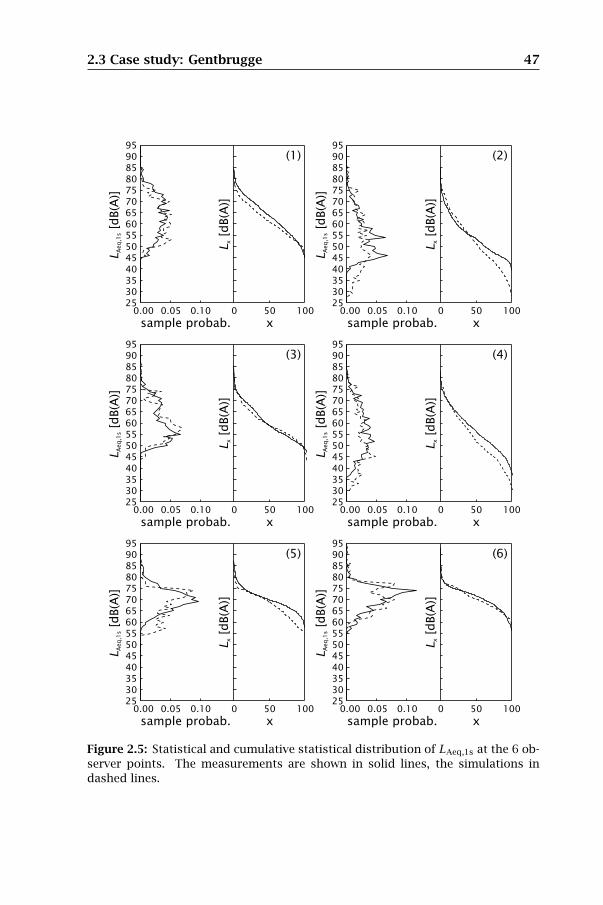
2.3 Case study: Gentbrugge 47
253035404550556065707580859095
1005000.100.050.00
Lx[d
B(A
)]
LA
eq,1
s[d
B(A
)]
xsample probab.
(6)
253035404550556065707580859095
1005000.100.050.00
Lx[d
B(A
)]
LA
eq,1
s[d
B(A
)]
xsample probab.
(5)
253035404550556065707580859095
1005000.100.050.00
Lx[d
B(A
)]
LA
eq,1
s[d
B(A
)]
xsample probab.
(4)
253035404550556065707580859095
1005000.100.050.00
Lx[d
B(A
)]
LA
eq,1
s[d
B(A
)]
xsample probab.
(3)
253035404550556065707580859095
1005000.100.050.00
Lx[d
B(A
)]
LA
eq,1
s[d
B(A
)]xsample probab.
(2)
253035404550556065707580859095
1005000.100.050.00
Lx[d
B(A
)]
LA
eq,1
s[d
B(A
)]
xsample probab.
(1)
Figure 2.5: Statistical and cumulative statistical distribution of LAeq,1s at the 6 ob-server points. The measurements are shown in solid lines, the simulations indashed lines.
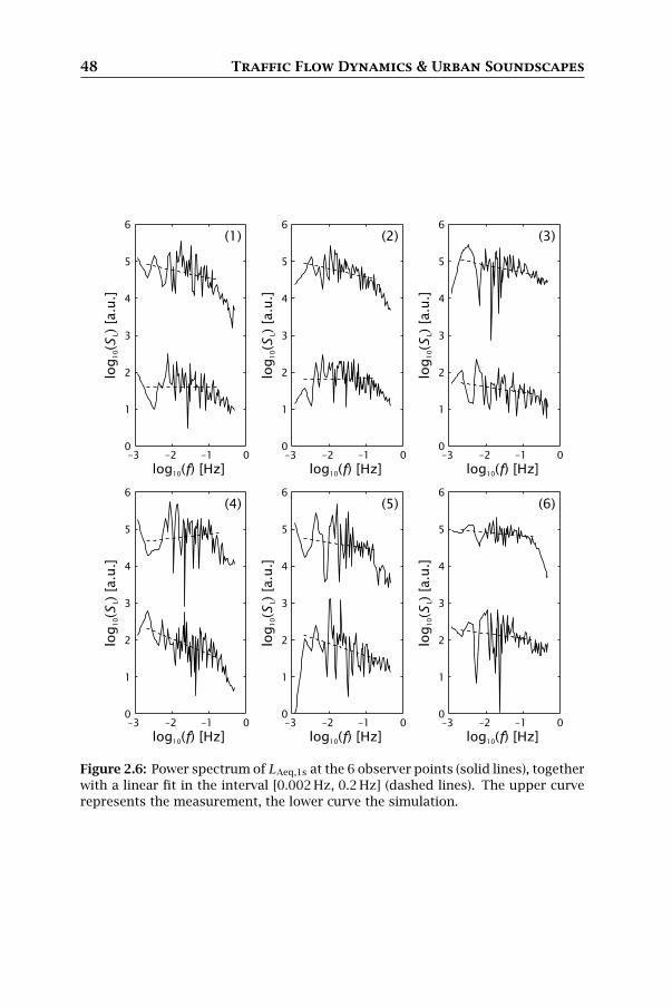
48 Traffic Flow Dynamics & Urban Soundscapes
0
1
2
3
4
5
6
0–1–2–3
log
()
[a.u
.]1
0L
S
log ( ) [Hz]10 f
(6)
0
1
2
3
4
5
6
0–1–2–3
log
()
[a.u
.]1
0L
S
log ( ) [Hz]10 f
(5)
0
1
2
3
4
5
6
0–1–2–3
log
()
[a.u
.]1
0L
S
log ( ) [Hz]10 f
(4)
0
1
2
3
4
5
6
0–1–2–3
log
()
[a.u
.]1
0L
S
log ( ) [Hz]10 f
(3)
0
1
2
3
4
5
6
0–1–2–3
log
()
[a.u
.]1
0L
S
log ( ) [Hz]10 f
(2)
0
1
2
3
4
5
6
0–1–2–3
log
()
[a.u
.]1
0L
S
log ( ) [Hz]10 f
(1)
Figure 2.6: Power spectrum of LAeq,1s at the 6 observer points (solid lines), togetherwith a linear fit in the interval [0.002 Hz, 0.2 Hz] (dashed lines). The upper curverepresents the measurement, the lower curve the simulation.

2.3 Case study: Gentbrugge 49
2.3.4 Sound field dynamics maps
As an example of a map showing the dynamics of the acoustic field, the
signalized junction on the main district road between observer points 5
and 6 was chosen. A rectangular grid of 200×200 observers with a spac-
ing of 0.5 m was put around the junction, at a height of 1.2 m. A 15-minute
time series of vehicle emissions was calculated using a timestep of 0.5 s.
Only noise emission of vehicles within a distance of 300 m from the center
of the grid was taken into account; exact vehicle positions were used. The
beamtrace propagation model was set to account for a maximum of 3 re-
flections and 1 diffraction. The calculation of a dynamic immission map
with these settings takes about 60 hours, using an amd Athlon at 1.7 GHz.
Figure 2.7 shows the resulting maps of LAeq,15min, LA5, LA5 − LA95 and
α. The major road, from the north-west to the south-east, carries about
5 times more traffic than the crossing minor road, which is reflected in
the signal times: the green (red) time on the major road is 65 s (30 s), on
the minor road it is 20 s (75 s). As a consequence, vehicles are standing
still for a much longer period on the minor road. This, together with the
discretization of the vehicle positions, characteristic to microsimulation
models, explains the dots appearing on the north-east arm of the junction.
In this context, one has to point out that the noise emission of vehicles
standing still is somehow overestimated using the Nord 2000 database,
because only noise measurements of vehicles driving at a non-zero speed
are available. In any case, only the observer points along the edge of the
road are of interest, for obvious reasons.
The LAeq,15min and LA5 maps show little variation along the footpath
and façade. The LA5 − LA95 map shows much more variation. Low values
can be found on the junction itself, because vehicles are passing by nearly
all the time, so both LA5 and LA95 are high. In the backyard shown in the
north, LA5 − LA95 is also low, but this time because LA5 and LA95 are both
low. In contrast, in the backyards to the east and in the southwest corner,
high LA5 − LA95 is observed. This can be explained by partial screening:
for some vehicle positions, traffic noise can reach these backyards directly.
The α map shows a more nuanced image. Values along the major road are
almost zero, implying random traffic dynamics. Values along the stoplines,
and in particular on the minor road, have a 1/f 1.5 to 1/f 2 behaviour, in-
dicating very predictable dynamics caused by stop-and-go traffic. In the
backyard in the north, the level fluctuations have a more 1/f to 1/f 1.5 be-
haviour, and is now more differentiated from the dynamics on the junction
itself.
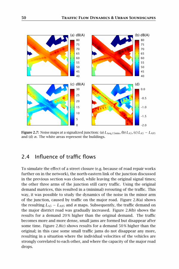
50 Traffic Flow Dynamics & Urban Soundscapes
0.0
–0.5
–1.0
–1.5
–2.0
(d)
30
25
20
15
10
5
0
dB(A)(c)
80
75
70
65
60
55
50
45
40
dB(A)(b)
80
75
70
65
60
55
50
45
40
dB(A)(a)
Figure 2.7: Noise maps at a signalized junction: (a) LAeq,15min, (b) LA5, (c) LA5 − LA95
and (d) α. The white areas represent the buildings.
2.4 Influence of traffic flows
To simulate the effect of a street closure (e.g. because of road repair works
further on in the network), the north-eastern link of the junction discussed
in the previous section was closed, while leaving the original signal times;
the other three arms of the junction still carry traffic. Using the original
demand matrices, this resulted in a (minimal) rerouting of the traffic. This
way, it was possible to study the dynamics of the noise in the minor arm
of the junction, caused by traffic on the major road. Figure 2.8(a) shows
the resulting LA5 − LA95 and α maps. Subsequently, the traffic demand on
the major district road was gradually increased. Figure 2.8(b) shows the
results for a demand 20 % higher than the original demand. The traffic
becomes more and more dense, small jams are formed but disappear after
some time. Figure 2.8(c) shows results for a demand 50 % higher than the
original; in this case some small traffic jams do not disappear any more,
resulting in a situation where the individual velocities of the vehicles are
strongly correlated to each other, and where the capacity of the major road
drops.
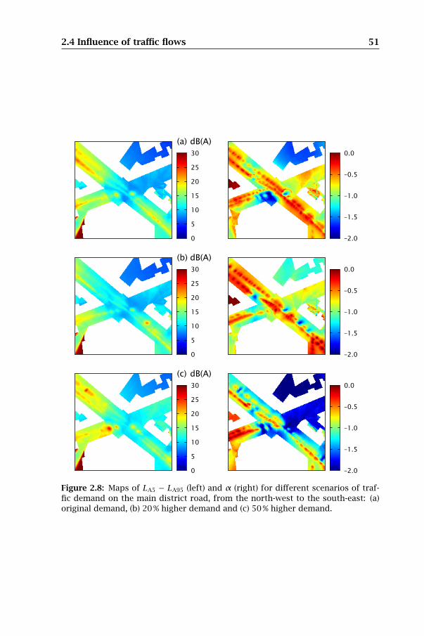
2.4 Influence of traffic flows 51
0.0
–0.5
–1.0
–1.5
–2.0
30
25
20
15
10
5
0
dB(A)(c)
0.0
–0.5
–1.0
–1.5
–2.0
30
25
20
15
10
5
0
dB(A)(b)
0.0
–0.5
–1.0
–1.5
–2.0
30
25
20
15
10
5
0
dB(A)(a)
Figure 2.8: Maps of LA5 − LA95 (left) and α (right) for different scenarios of traf-fic demand on the main district road, from the north-west to the south-east: (a)original demand, (b) 20 % higher demand and (c) 50 % higher demand.

52 Traffic Flow Dynamics & Urban Soundscapes
For the different demands, a small but visible trend can be found on
the LA5 − LA95 maps in the no-traffic arm of the junction. However, when
considering theαmaps, a clearer evolution is visible. The original demand,
which does not display any jams, results in a rather chaotic behaviour with
α ≈ −0.5. The 20 % higher demand, near the traffic jam transition point,
shows a more 1/f behaviour in the closed street; this behaviour is now also
found in the northern backyard. When traffic demands are still further in-
creased, the clustering and jamming of the vehicles results in a 1/f 1.5 to
1/f 2 behaviour of the noise immission spectrum. At the façades along the
major road and away from the junction a 1/f spectrum is still observed.
This corresponds with the earlier findings of 1/f behaviour in the power
spectrum of traffic flow in microsimulation models near the jamming tran-
sition point [55, 350], which is reflected here in the noise immission spec-
trum.
If anything, these few scenario calculations show that taking into ac-
count traffic noise dynamics makes noise maps much more sensitive to
minor changes in traffic.
2.5 Conclusions
A tool for dynamic traffic noise prediction, based on microsimulation of the
traffic in an urban neighbourhood, coupled with a state-of-the-art beam-
trace propagation model was introduced. The unique feature of this ap-
proach is that it allows to estimate the effect of traffic flow management on
noise in a much wider area than previous models. The model was compared
with measurements of LAeq,1s over 15 minutes and in general good agree-
ment was found for all the statistical properties of this fluctuating noise
level. Further improvement could include the introduction of corrections
on the emission of accelerating and decelerating vehicles, the introduction
of correct motorcycle and tram emission spectra, and the implementation
of diffuse reflections in the propagation model.
A method for evaluating the patterns in time variations of a series of
dynamic noise immission values, based on the power spectrum of sound
amplitude fluctuations, was proposed. A combination of this new indi-
cator with more conventional indicators based on statistical noise levels
allows to monitor the effect of traffic on the urban soundscape more ac-
curately. Based on these indicators, it was shown that minor changes in
traffic (possibly caused by flow management) have a much larger effect on
the soundscape than expected on the bases of average emission and im-
mission mapping.
Chapter3
Microsimulation based
Corrections on the Noise
Emission near Intersections
B. De Coensel, D. Botteldooren,
F. Vanhove and S. Logghe
Accepted for publication in Acta Acustica united with Acustica.
« « «
In this chapter, the variation in noise immission in the vicinity of in-
tersections, caused by the typical deceleration and acceleration pro-
files of vehicles, is studied. A methodology for deriving intersection
corrections for traditional macroscopic traffic noise prediction mod-
els is outlined. The research described in this chapter was conducted
in the framework of the imagine project [151], funded by the Sixth
Framework Programme of the European Community. Results of this
research were presented at the 6th European Conference on Noise
Control [73].
3.1 Introduction
Several national standards exist for the prediction of road traffic noise (for
a review, see e.g. [300]). Most of these engineering models assume that
roads can be divided into sections of considerable length where the vehicle
flow can be considered homogeneous. Traffic flow calculations are usually
based on traffic simulation models which consider average flow parame-
ters. Traditionally, the sound emission caused by the traffic on each seg-

54 Corrections on the Noise Emission near Intersections
ment is modeled as a function mainly of the average vehicle speed and the
traffic flow rate; most modern engineering models differentiate between
the emissions produced by different types of vehicles [319].
However, the assumption of a spatially homogeneous traffic flow does
not hold in the vicinity of junctions and other types of traffic delaying struc-
tures such as speed bumps; segments of constant noise emission have to
be made smaller. In addition, average vehicle speeds calculated by macro-
scopic traffic simulation models become unreliable. For example, in the
case of a signalized junction, a fraction of the traffic has to slow down to a
halt, while another fraction of the traffic can cross the intersection without
slowing down considerably. Finally, noise emission of stop-and-go traffic
depends highly on vehicle acceleration, a parameter which can often not
be reported by traditional traffic flow simulation models.
Because of these complications, the influence of intersections, and more
in general of interrupted traffic flows, is evaluated mostly in a pragmatic
way. The French prediction model, consisting of the Guide du Bruit [239]
and the NMPB-96 propagation method [240], the UK CRTN prediction
method [65] and the Swiss SonRoad road traffic noise model [143] do not in-
clude the impact of intersections at all — although recently efforts were un-
dertaken to update the French model for different driving conditions [23].
In the Nordic model [181, 167], the use of a correction on the vehicle noise
emission for continuous acceleration (after a crossing) and continuous de-
celeration (before a crossing) is proposed; however no input data for these
driving conditions is available, and the model thus recommends to use only
the cruising vehicle emission values. The Dutch RMW2002 model [272] in-
cludes an immission correction for intersections, depending on the inter-
section type and the diurnal traffic intensity. This correction can be at most
2.4 dB(A) at the center of the intersection and decreases linearly with the
distance, for up to a distance of 150 m. The German RLS90 model [271] also
includes an immission correction term for intersections with traffic lights,
for up to a distance of 100 m from the intersection. The non-European
models of the us [213] and Japan [303, 345] both introduce a correction on
the noise emission for transient driving conditions near intersections.
In spite of the fact that intersection corrections are only marginally
taken into account in most prediction models in use today, there has been a
reasonably amount of research on the topic of noise (reduction) from traffic
management in the last three decades; a review can be found in [82]. In the
uk, the earliest studies on interrupted traffic flows focused on L10 measure-
ments nearby conventional intersections [120] and roundabouts [194, 195].
In general it was found that the noise from the accelerating traffic streams
was within 1 dB(A) of the free flow level. In the early 1980’s, basic computer
models were introduced to predict traffic noise. In [83, 168, 169, 264], sim-

3.1 Introduction 55
ulation models for LA10 for various types of interrupted flows were intro-
duced. In a French study [100], a computer model for determining the noise
radiated by a single vehicle approaching traffic lights was demonstrated. A
Dutch model was also published [159], which was able to predict percentile
noise levels of interrupted traffic flows in built-up environment. The prop-
agation part for this model was based on transfer functions measured in
a scale model. By the same author, a method for measuring the decrease
and increase of vehicle noise levels at intersections was published [236].
After a less fruitful period, the study of noise at intersections gained
renewed interest in the second half of the 1990’s, possibly driven by new
advances in the field of traffic modeling and the introduction of microsim-
ulation models in traffic flow prediction. The STRADABruit model [191],
developed by the French National Institute for Transport and Safety Re-
search (inrets), is based on a fluid dynamics macroscopic traffic model,
modified to be able to represent transitional flow states at intersections,
and coupled with a vehicle emission model based on test track measure-
ments. This model was validated with measurements at a signalized in-
tersection [189], and has recently been extended with a microsimulation
model for special types of vehicles, and a more advanced propagation
model [190]. Oshino et al. [247] made a coupling between a simple mi-
crosimulation model and a noise emission model for individual vehicles;
a validation with measurements near various types of signalized intersec-
tions was also published [248, 301]. In the most recent models, a microsim-
ulation model is coupled with an individual vehicle noise emission model
and an advanced propagation model. The model developed at the Univer-
sity of Oviedo [252, 351], as well as the models developed at the University
of Leeds [198, 123, 122] and at Ghent University [72, 39], make it possible to
assess (percentile) traffic noise levels at (signalized) intersections in com-
plex urban built-up environments. These models were recently updated
for the latest Harmonoise vehicle noise emission model [166].
Measurements of the influence of the replacement of traffic lights by
roundabouts on noise levels are discussed in [12], and a regression model
for assessing their impact is deduced. It is found that, in ideal conditions, a
reduction in LAeq,24h of 1 to 4 dB can be achieved. A semi-analytical method
to assess the noise impact of a roundabout is proposed in [255]; measure-
ments are used to predict the kinematic parameters of vehicles traveling
on the roundabout. In [278], road traffic noise was measured before and
after the installation of traffic lights. In general, higher levels were found
in the vicinity of the intersection, while lower levels were found at some
distance from the lights. The last decade, there was also a more theoreti-
cal movement in traffic intersection noise research. In [311], a formula for
the noise emitted from vehicles at a roundabout is derived analytically. A
56 Corrections on the Noise Emission near Intersections
comprehensive number of analytical studies were performed by Kokowski
and Makarewicz [179, 206, 178, 205], on the noise emitted from vehicles
at signalized intersections and roundabouts.
Traffic noise prediction models that aim to be accurate in the vicinity of
interrupted traffic flows, will have to model the temporal and spatial evolu-
tions of vehicle speeds and accelerations. Microsimulation models can in-
corporate these dynamic effects. In recent efforts to harmonize traffic noise
prediction on a European level [151], microsimulation models therefore are
included. However, the main difficulties associated with microsimulation
modeling are the large amount of detailed data on traffic flows needed and
the fact that constructing and calibrating the model is time-consuming and
only feasible for small to medium sized regions. When traffic noise pre-
diction is based on a traffic model that does not simulate the dynamics of
intersections, a correction could be applied to incorporate the effects on
noise emissions.
In this chapter, a possible method to derive such corrections will be
described, based on microsimulation results. Since it is not possible to
simulate all conceivable intersection configurations and scenarios, a num-
ber of simple intersection scenarios were considered, in which a limited
number of parameters were varied. This limits the applicability of the re-
sults described in this chapter. However, in a typical real life study area, the
variation in intersection types will not be very large, so the methodology
desribed in this chapter can easily be used to study the typical intersections
in the study region, and to extrapolate the results to the whole network
under study. In Section 3.2, the general methodology will be described;
Section 3.3 discusses some insights gained into the specific dynamics of
the noise immission near different types of intersections. Finally, intersec-
tion corrections that can be applied in case no microsimulation is available
will be derived in Section 3.4. A spatial approach will be used, in which in-
bound and outbound lanes are divided into deceleration, queuing, stopline
and acceleration zones.
3.2 Methodology
3.2.1 Microsimulation models
To gain insight into the specific dynamics of the noise emission near dif-
ferent types of traffic junctions, a number of microscopic traffic simula-
tion models were constructed. All models consisted of an intersection of
a major road (inbound traffic flow of DM vehicles·h−1) and a minor road
(inbound traffic flow of Dm vehicles·h−1). A schematic view can be found

3.2 Methodology 57
Dm
DM
Dm
DM
roundabouttraffic lights
prioritypriority–to–the–right
Figure 3.1: The four intersection types considered.
in Figure 3.1. Both the major road and the minor road only have one lane
in each direction, and the speed is limited to 70 km·h−1 on both roads.
Four different intersection types (I) were considered: an intersection with
a priority-to-the-right rule; an intersection where the major road has prior-
ity ; an intersection with traffic lights and a roundabout.
By varying the traffic demands on the major and minor roads, differ-
ent scenarios with calm, normal and busy traffic were created; six combi-
nations were chosen (data can be found in Table 3.1). Three variations in
traffic composition, with a percentage F of heavy vehicles equal to 5 %, 10 %
or 20 %, were considered. The number of scenarios was further increased
by taking into account the percentage of the traffic that turns left or right
(turning rate R), as this parameter may also influence congestion on cer-
tain types of intersections. Two situations were considered: one with 20 %
turning traffic on both major and minor roads (10 % to the left and 10 %
to the right), and one with 40 % turning traffic (20 % to the left and 20 % to
the right). The total number of unique traffic scenarios is then equal to
#I × #(DM ,Dm)× #F × #R = 4× 6× 3× 2 = 144.
The microsimulation model parameters, such as the aggression, aware-
ness and reaction time distribution of the vehicle drivers, the queue gap
distance, the mean target headway between a vehicle and a following vehi-
cle, the signposting distance etc., were not varied in this case study; stan-
dard values were used. Although these parameters have a significant in-
fluence on traffic dynamics near intersections, it is assumed that they do
not vary much within a case study network. These parameters will have to
be adjusted for the specific case study situation to which the methodology
described in this chapter is applied.
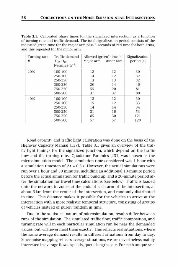
58 Corrections on the Noise Emission near Intersections
Table 3.1: Calibrated phase times for the signalized intersection, as a functionof turning rate and traffic demand. The total signalization period consists of theindicated green time for the major arm plus 3 seconds of red time for both arms,and this repeated for the minor arm.
Turning rate Traffic demand Allowed (green) time [s] SignalizationR DM -Dm Major arm Minor arm period [s]
[vehicles·h−1]
20 % 100-100 12 12 30250-100 14 12 32250-250 13 13 32500-250 26 14 46750-250 55 20 81500-500 37 37 80
40 % 100-100 12 12 30250-100 15 12 33250-250 14 14 34500-250 31 16 53750-250 85 30 121500-500 57 57 120
Road capacity and traffic light calibration was done on the basis of the
Highway Capacity Manual [137]. Table 3.1 gives an overview of the traf-
fic light timings for the signalized junction, which depend on the traffic
flow and the turning rate. Quadstone Paramics [251] was chosen as the
microsimulation model. The simulation time considered was 1 hour with
a simulation timestep of ∆t = 0.5 s. However, the actual simulations were
run over 1 hour and 30 minutes, including an additional 10-minute period
before the actual simulation for traffic build up, and a 20-minute period af-
ter the simulation for travel time calculations (see below). Traffic is loaded
onto the network in zones at the ends of each arm of the intersection, at
about 3 km from the center of the intersection, and randomly distributed
in time. This distance makes it possible for the vehicles to arrive at the
intersection with a more realistic temporal structure, consisting of groups
of vehicles instead of purely random in time.
Due to the statistical nature of microsimulation, results differ between
runs of the simulation. The simulated traffic flow, traffic composition, and
turning rate will in each particular simulation run be near the demanded
values, but will never meet them exactly. This reflects real situations, where
the same average demand results in different situations from day to day.
Since noise mapping reflects average situations, we are nevertheless mainly
interested in average flows, speeds, queue lengths, etc. For each unique sce-

3.2 Methodology 59
nario, results were therefore averaged over 5 simulation runs with different
seed values, to enable statistically sound conclusions. Average actual sce-
nario traffic flows QM and Qm and average percentages of heavy traffic F
were extracted from the simulation runs, for each lane separately, using
a dedicated Paramics plugin. These values may differ from the nominal
values described in the previous section (which were used as model input
parameters). However, the differences are only substantial for the traffic
flows in the case of congestion (emphasized by a different notation for de-
mand and flow); in this case the actual traffic flow Qx will be less than the
traffic demand Dx put forward. Nominal values of Dx , F and R will be
used to simplify the discussion in Section 3.3; the averaged values of Qxand F , extracted from the actual simulations, will be used when deriving
corrections in Section 3.4.
3.2.2 Calculation of travel times
Macroscopic traffic models often translate the effect of the presence of
crossings to an additional travel time on this part of the network. Travel
time is therefore a useful parameter in an engineering type correction for
traffic noise emission at and immission near intersections. Calculation of
travel times, averaged over 1 hour of simulation, was made on the basis
of travel time data reported by Paramics, for each lane separately. The
average is calculated for all trips departing within the 1-hour simulation
period. This means that a number of vehicles arrive at their destination
zone after the actual simulation period has ended (especially in the case of
congestion). This way, the travel times can be compared to travel times gen-
erated by static assignment models, in which it is assumed that all traffic
completes its journey through the network within the simulation period.
However, one has to be careful when considering travel times returned
by macroscopic models. The deceleration of vehicles approaching the in-
tersection results in an actual average speed which is lower than the free
flow limit speed. In macroscopic models, this is reflected by the travel
time associated with the (inbound) link of the intersection. The extra travel
time associated with the intersection itself therefore only reflects possible
queues and congestion. Because the travel time associated with the inter-
section itself (noted T ) is considered in this case study, the travel times
corresponding to the case where there are no queues (the zero extra in-
tersection associated travel time situation) have to be subtracted from the
travel time results obtained through microsimulation. For this, a fifth in-
tersection type was added as a reference: a simple intersection without
priority rules. Simulations of all scenarios for this reference network were
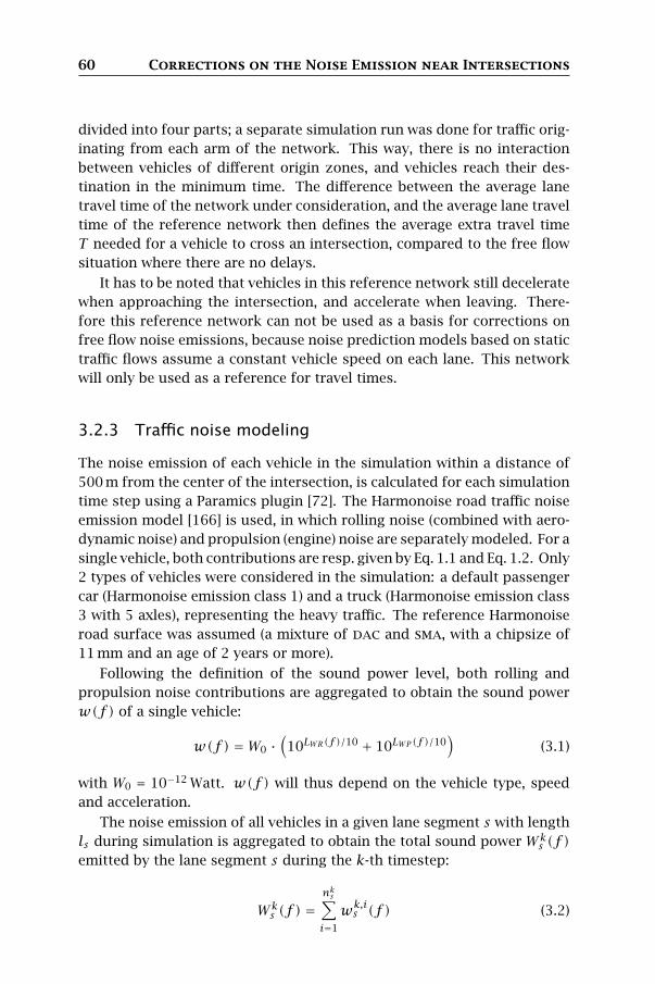
60 Corrections on the Noise Emission near Intersections
divided into four parts; a separate simulation run was done for traffic orig-
inating from each arm of the network. This way, there is no interaction
between vehicles of different origin zones, and vehicles reach their des-
tination in the minimum time. The difference between the average lane
travel time of the network under consideration, and the average lane travel
time of the reference network then defines the average extra travel time
T needed for a vehicle to cross an intersection, compared to the free flow
situation where there are no delays.
It has to be noted that vehicles in this reference network still decelerate
when approaching the intersection, and accelerate when leaving. There-
fore this reference network can not be used as a basis for corrections on
free flow noise emissions, because noise prediction models based on static
traffic flows assume a constant vehicle speed on each lane. This network
will only be used as a reference for travel times.
3.2.3 Traffic noise modeling
The noise emission of each vehicle in the simulation within a distance of
500 m from the center of the intersection, is calculated for each simulation
time step using a Paramics plugin [72]. The Harmonoise road traffic noise
emission model [166] is used, in which rolling noise (combined with aero-
dynamic noise) and propulsion (engine) noise are separately modeled. For a
single vehicle, both contributions are resp. given by Eq. 1.1 and Eq. 1.2. Only
2 types of vehicles were considered in the simulation: a default passenger
car (Harmonoise emission class 1) and a truck (Harmonoise emission class
3 with 5 axles), representing the heavy traffic. The reference Harmonoise
road surface was assumed (a mixture of dac and sma, with a chipsize of
11 mm and an age of 2 years or more).
Following the definition of the sound power level, both rolling and
propulsion noise contributions are aggregated to obtain the sound power
w(f) of a single vehicle:
w(f) = W0 ·(10LWR(f )/10 + 10LWP (f )/10
)(3.1)
with W0 = 10−12 Watt. w(f) will thus depend on the vehicle type, speed
and acceleration.
The noise emission of all vehicles in a given lane segment s with length
ls during simulation is aggregated to obtain the total sound power Wks (f )
emitted by the lane segment s during the k-th timestep:
Wks (f ) =
nks∑
i=1
wk,is (f ) (3.2)

3.2 Methodology 61
with nks the number of vehicles within the lane segment s on the k-th
timestep and wk,is (f ) the sound power emitted by the i-th vehicle within
the lane segment s during the k-th timestep. The hourly averaged sound
power Ws(f ) emitted by the lane segment s is then obtained by
Ws(f ) =∆t
tsim·
tsim/∆t∑
k=1
Wks (f ) (3.3)
with tsim = 3600 s the total simulation duration and tsim/∆t the total num-
ber of timesteps in the simulation.
Finally, the hourly averaged A-weighted sound power level LW,s emitted
by the lane segment s is given by
LW,s = 10 · log10
(∑f A(f) ·Ws(f )
W0
)(3.4)
with A(f) the A-weighting correction factor for the one-third octave band
with center frequency f . We note that the hourly occupancy Qs of the
segment s is given by
Qs =
tsim/∆t∑
k=1
nks (3.5)
and is related to the traffic flow on the segment s. Traffic flow and occu-
pancy are not equal, since vehicles standing still in the segment may be
counted more than once. In free flow condition however, both are pro-
portional quantities. Using Eqs. 3.2, 3.3 and 3.5, Eq. 3.4 can be rewritten
as
LW,s = 10 · log10
(∆t
tsim·
⟨wA,s
⟩
W0
)+ 10 · log10 (Qs) (3.6)
where
⟨wA,s
⟩=
1
Qs
∑
f
tsim/∆t∑
k=1
nks∑
i=1
A(f) ·wk,is (f ) (3.7)
is the average A-weighted sound power of a single vehicle on the lane seg-
ment s.
To obtain a good spatial resolution, the segment length should be kept
low. Therefore, for the calculation of the corrections in Section 3.4 (based
on LW,s ), a segment length ls = 5 m was used, in which at most only one vehi-
cle fits (nks = 0 or 1). For the calculation of the noise maps in Section 3.3, the
noise immission level LAeq,1h was calculated using the iso 9613 propaga-
tion model [157] (hard surface), in a square area of 200 m × 200 m without
buildings, departing from the hourly averaged sound power Ws(f ) for all
lane segments.

62 Corrections on the Noise Emission near Intersections
3.3 Microsimulation results
3.3.1 Influence of scenario parameters on travel time
Table 3.2 summarizes the average extra travel time T , for both the major
and minor arms of the intersection. One can see that for all networks,
travel time increases with increasing traffic demand. For the major arm of
the intersection, the priority junction will obviously be the best choice in all
cases. For the minor arm this would be the roundabout, which also seems
to be the overall best intersection layout. For low traffic demands, traffic
lights have a clear disadvantage, for high traffic demands the priority-to-
the-right junction is the worst choice. A t-test revealed that traffic compo-
sition F and turning rate R did not have a significant influence on travel
time (p > 0.1); results were therefore averaged over F and R in Table 3.2.
Some intersection scenarios resulted in congestion: no stable traffic
situation was achieved on the major and/or minor inbound lanes during
simulation (queue lengths grow during the full simulation due to jams). In
this case the calculated travel times have high variance between different
simulation runs and become unreliable. However, these types of intersec-
tions will in practice probably never be used for these traffic volumes. In
some scenarios, the formation of a queue has an impact on noise emission
(the effect will be quantified in Section 3.4). Small queues can be formed
in other situations, but their impact on noise emission will be negligible.
E.g. for the intersection with traffic lights, at lower traffic demands still a
fraction of the traffic can traverse the intersection without slowing down;
the noise emission of these vehicles will then be dominant in the queuing
area. Limits are not clear, but as a rule of thumb derived from Table 3.2,
one can say that important queues are formed when T > 25 s, and that the
network is congested when T > 100 s.
3.3.2 Influence of scenario parameters on total noise emission
To have an impression of the total noise generated on the intersection, the
intersection can be considered as one large emission segment. For this,
the time-varying noise emission of all vehicles within a given radius from
the center of the intersection was aggregated and averaged over 1 hour,
using equations 3.2 to 3.4. This makes it possible to compare different
scenarios using a single noise emission value. From Eq. 3.6 it can be seen
that, in free flow, this sound power level increases as 10 log(QM + Qm)
since Qs ∼ QM +Qm. Furthermore, the total noise emission also depends
on the average A-weighted sound power of a single vehicle and thus on the

3.3 Microsimulation results 63
Table 3.2: Average extra travel time T (in seconds).
Traffic demand Priority-to-the-right PriorityDM -Dm Major arm Minor arm Major arm Minor arm[vehicles·h−1]
100-100 3.9 3.8 0.4 3.2250-100 6.8 5.9 0.4 4.4250-250 24.9 22.7 0.7 7.9500-250 408.1∗∗ 72.8∗ 1.2 37.6∗
750-250 650.6∗∗ 93.1∗ 3.1 311.3∗∗
500-500 559.8∗∗ 484.6∗∗ 1.5 439.5∗∗
Traffic lights RoundaboutMajor arm Minor arm Major arm Minor arm
100-100 8.1 8.1 1.6 1.4250-100 8.9 8.8 1.8 1.3250-250 10.5 9.8 2.4 2.2500-250 11.4 18.9 4.0 2.9750-250 25.7∗ 50.7∗ 8.0 4.7500-500 36.0∗ 38.5∗ 6.6 5.6∗Queues with impact on average noise emission are formed;∗∗Congested lane.
traffic composition F . Turning rateR again was found to have no significant
influence (p > 0.1) on total noise emission in this case study.
The resulting total noise emission will however also depend on the ag-
gregation size. The larger the aggregation radius, the higher the total noise
emission, but also the smaller the differences between different types of
intersections. To see this, one has to compare the four intersection types
with the imaginary situation in which the two roads cross each other with-
out any interference, and all vehicles drive with the free flow speed on the
whole “intersection”. This case can be seen as the absence of any influence
of an intersection on the traffic flow. Differences in the noise emission
between the four intersections and the imaginary free flow situation are
due to the typical acceleration and deceleration profiles near intersections,
the lower speeds, and to the fact that it will take a longer time to cross an
actual intersection compared to the imaginary free flow “intersection”. At
larger distance from the center of the intersection, all vehicles will drive at
the free flow speed, independent of the type of intersection.
It is interesting to look at the aggregation radius needed to make the
difference in total noise emission between the different intersection types
and the free flow situation smaller than 1 dB(A). Table 3.3 shows that this
radius varies between 70 and 170 m for the non-congested scenarios (cor-

64 Corrections on the Noise Emission near Intersections
Table 3.3: Aggregation radius (in m) at which the difference in total noise emis-sion between the different intersection types and the free flow situation becomessmaller than 1 dB(A).
Traffic demand Traffic composition FDM -Dm 5 % 10 % 20 %[vehicles·h−1]
100-100 160 100 160250-100 140 80 150250-250 120 70 140500-250 150 150 150750-250 >500 >500 >500500-500 170 120 160
responding to a segment length of 140 to 340 m). When noise maps are
drawn with this resolution, one can have 1 dB(A) accuracy on average noise
exposure, without having to bother about intersection corrections. The
aggregation radius needed for this accuracy is smallest for intermediate
traffic demands and a percentage of heavy vehicles of 10 %. In the case of
heavy congestion, it was found that 1 dB(A) accuracy could not be achieved
with an aggragation radius smaller than 500 m.
3.3.3 Influence of scenario parameters on noise immission
As an example, Figure 3.2 shows a noise map of the signalized intersec-
tion, together with the differences in noise immission level with the other
3 types of intersections considered. As can be seen, the intersection type
has a large influence on vehicle speed and acceleration, and as a conse-
quence on local noise immission. Differences in local LAeq,1h can be up
to 2 to 3 dB(A) with the priority-to-the-right and priority intersection. The
noise map of the priority intersection seems to reproduce the results found
in [278] and discussed in the introduction; however, only for the prior-
ity arm. The large differences for the roundabout can be attributed to
the different physical road layout and to the higher average speeds of ap-
proaching traffic on signalized intersections. At some distance from the
center, a reduction of several dB(A) is found for the roundabout compared
with the signalized intersection, which is in agreement with earlier mea-
surements [12]. For the priority junction, noise emission is larger along
the major road because vehicles do not have to slow down, but smaller
near the stoplines and on the minor road where all vehicles slow down or
stop. For the priority-to-the-right junction, the opposite is true: the highly
interrupted traffic results in slightly higher noise levels near the center

3.3 Microsimulation results 65
4
2
0
–2
–4
dB(A)(d)
85
80
75
70
65
60
dB(A)(c)
4
2
0
–2
–4
dB(A)(b)
4
2
0
–2
–4
dB(A)(a)
Figure 3.2: Noise maps (LAeq,1h) of (a) the difference between the priority-to-the-right and the signalized intersection, (b) the difference between the priority andthe signalized intersection, (c) the signalized intersection and (d) the differencebetween the roundabout and the signalized intersection (DM = 250 vehicles·h−1,Dm = 100 vehicles·h−1, F = 20 %, R = 20 %).
and stoplines of the intersection, but lower levels at some distance. From
this, it can be concluded that noise emission corrections should be made
spatially dependent. These conclusions remain quantitatively valid for all
non-congested scenarios considered.
So far, only the energetic mean of the results of the 5 simulation runs
was presented. In Figure 3.3, the standard deviation of the 5 simulation
runs that led to the maps in Figure 3.2 are shown. The small dots appearing
along the lanes are related to the discretization involved in microsimulation
models. The largest modeling uncertainty can be found at the locations
where the traffic is most interrupted, and where small jams are formed,
mostly on the minor arms of the intersection. There may be two expla-
nations for this. Firstly, the dependence on acceleration behaviour and
corresponding increase in sound levels is larger in these areas. Secondly,
and probably more importantly, the length of the queue waiting to enter
the intersection is very chaotic and unpredictable, also on real junctions
with approximately this traffic load. Thus, provided that the number of
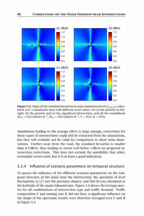
66 Corrections on the Noise Emission near Intersections
1.2
1.0
0.8
0.6
0.4
0.2
0.0
dB(A)(d)
1.2
1.0
0.8
0.6
0.4
0.2
0.0
dB(A)(c)
1.2
1.0
0.8
0.6
0.4
0.2
0.0
dB(A)(b)
1.2
1.0
0.8
0.6
0.4
0.2
0.0
dB(A)(a)
Figure 3.3: Maps of the standard deviation in noise immission level (LAeq,1h), calcu-lated over 5 simulation runs with different seed values, for (a) the priority-to-the-right, (b) the priority and (c) the signalized intersection, and (d) the roundabout(DM = 250 vehicles·h−1, Dm = 100 vehicles·h−1, F = 20 %, R = 20 %).
simulations leading to the average effect is large enough, corrections for
these types of intersections could still be extracted from the simulations,
but they will certainly not be valid for comparison to short term obser-
vations. Further away from the road, the standard deviation is smaller
than 0.5 dB(A), thus leading to errors well below 1 dB(A) on proposed in-
tersection corrections. This does not exclude the possibility that other,
systematic errors exist, but it is at least a good indication.
3.3.4 Influence of scenario parameters on temporal structure
To assess the influence of the different scenario parameters on the tem-
poral structure of the noise near the intersection, the spectrum of level
fluctuations SL(f ) (see the previous chapter, and Part II) was calculated at
the kerbside of the major inbound arm. Figure 3.4 shows the average spec-
tra for all combinations of intersection type and traffic demand. Traffic
composition F and turning rate R did not have a significant influence on
the shape of the spectrum; results were therefore averaged over F and R
in Figure 3.4.
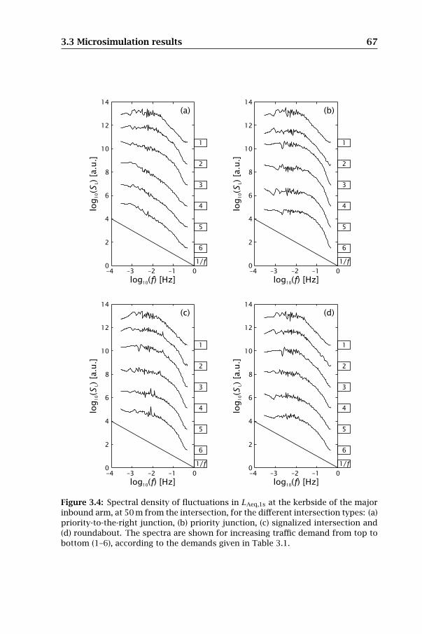
3.3 Microsimulation results 67
14
12
10
8
6
4
2
0–2 –1 0–3–4
1/f
6
5
4
3
2
1
log
(10
SL)
[a.u
.]
log ( ) [Hz]10 f
(d)14
12
10
8
6
4
2
0–2 –1 0–3–4
1/f
6
5
4
3
2
1
log
(10
SL)
[a.u
.]
log ( ) [Hz]10 f
(c)
14
12
10
8
6
4
2
0–2 –1 0–3–4
1/f
6
5
4
3
2
1
log
(10
SL)
[a.u
.]
log ( ) [Hz]10 f
(b)14
12
10
8
6
4
2
0–2 –1 0–3–4
1/f
6
5
4
3
2
1
log
(10
SL)
[a.u
.]
log ( ) [Hz]10 f
(a)
Figure 3.4: Spectral density of fluctuations in LAeq,1s at the kerbside of the majorinbound arm, at 50 m from the intersection, for the different intersection types: (a)priority-to-the-right junction, (b) priority junction, (c) signalized intersection and(d) roundabout. The spectra are shown for increasing traffic demand from top tobottom (1–6), according to the demands given in Table 3.1.

68 Corrections on the Noise Emission near Intersections
For low traffic volume, the shape of the spectrum, and as a consequence
the temporal structure of the soundscape, is independent of the intersec-
tion type, and approximates the theoretical shape for vehicles passing by
randomly (see Section 6.4.2). For the least obstructed intersection types
(priority junction, roundabout and signalized junction), this shape is main-
tained when the traffic flow increases. In the case of the signalized intersec-
tion, peaks are visible, corresponding to the traffic light period (Table 3.1).
For the priority-to-the-right intersection, which is the most obstructed type,
increasing the traffic demand results in a much more 1/f shape of the spec-
trum, as congestion is reached. This is conform to findings in literature,
which will be discussed in Section 4.3.2.
3.4 Emission corrections
In this section, an onset is given in formulating corrections, which can be
applied to the noise emission obtained through the use of macroscopic traf-
fic models that do not take into account traffic dynamics on intersections.
As already mentioned in the previous section, some intersection scenarios
resulted in a congested major and/or minor inbound lane; these lanes are
excluded from the correction analysis. The outbound lanes of these con-
figurations were nevertheless taken into account, since no jams are formed
there. The roundabout is not taken into account for the correction analy-
sis, as the layout of this type of intersection differs highly from the other
3 types.
3.4.1 Noise emission profile
It is assumed that the noise emission, obtained through the use of macro-
scopic traffic modeling, consists of a series of static sound sources with
hourly averaged A-weighted sound power level LW,s (Eq. 3.4), associated to
segments of a lane of the road. Figure 3.5 shows an example of a simu-
lated noise emission profile LW,s along a lane of the intersection; the other
scenarios produce similar profiles. A segment length of 5 m was used, as
explained in Section 3.2.3. A larger segment length would obfuscate the
fine structure of local noise emission near the center of the intersection,
while a smaller segment length would not give additional information, since
at most 1 vehicle can be in each segment at any time. One could subtract
10 log10(5) ≈ 7 dB(A) to get the noise emission per lane in segments of 1 m
length; this has however no implications for the derivation of the correction
factors, as only differences in sound power level will be considered.

3.4 Emission corrections 69
84
82
80
78
76
74
7230025020015010050050100150200250300
distance from intersection center [m]
em
issio
n p
rofi
le [
dB(A
)]
Figure 3.5: Noise emission profile LW,s for the inbound (left) and outbound(right) lane of the major arm of the priority-to-the-right intersection (DM = Dm= 100 vehicles·h−1, F = 5 %, R = 40 %), averaged over 5 simulation runs.
At larger distances from the junction the noise emission is indepen-
dent of the location, as can be expected for cruising vehicles. The hourly
averaged A-weighted sound power level emitted by a segment s at large
distance from the junction will be referred to as LW,s . The corresponding
value of the average A-weighted sound power of a single vehicle cruising at
large distance from the junction is 〈wA〉. Noise corrections will be based
on the limit value LW,s , as it is assumed that this is the usual emission out-
put of traffic noise prediction based on a macroscopic model. Closer to the
intersection (which is at the origin in Figure 3.5), different regions can be
observed.
On the inbound lane, the noise emission starts to drop at some distance
from the intersection, as vehicles start to decelerate. Just before the inter-
section (at the stopline), a small discontinuous peak is observed, due to
the high engine speed and associated acceleration of departing vehicles,
which is accounted for in the acceleration correction to the propulsion
contribution (Section 1.3.3). Beyond the stopline, the average noise emis-
sion decreases as the acceleration decreases. When a significant queue is
formed on the inbound lane, the vehicle acceleration peak is spread out in
a larger area before the stopline, which we will call the queuing zone. On
the outbound lane the sound level rises to the cruising value over a limited
distance, due to the increasing average vehicle speed.
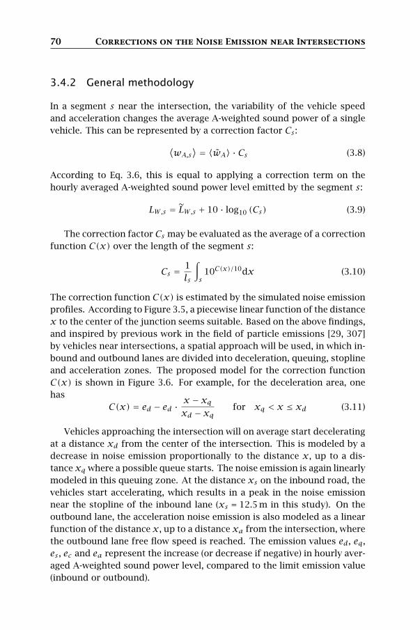
70 Corrections on the Noise Emission near Intersections
3.4.2 General methodology
In a segment s near the intersection, the variability of the vehicle speed
and acceleration changes the average A-weighted sound power of a single
vehicle. This can be represented by a correction factor Cs :
⟨wA,s
⟩= 〈wA〉 · Cs (3.8)
According to Eq. 3.6, this is equal to applying a correction term on the
hourly averaged A-weighted sound power level emitted by the segment s:
LW,s = LW,s + 10 · log10 (Cs) (3.9)
The correction factor Cs may be evaluated as the average of a correction
function C(x) over the length of the segment s:
Cs =1
ls
∫
s10C(x)/10dx (3.10)
The correction function C(x) is estimated by the simulated noise emission
profiles. According to Figure 3.5, a piecewise linear function of the distance
x to the center of the junction seems suitable. Based on the above findings,
and inspired by previous work in the field of particle emissions [29, 307]
by vehicles near intersections, a spatial approach will be used, in which in-
bound and outbound lanes are divided into deceleration, queuing, stopline
and acceleration zones. The proposed model for the correction function
C(x) is shown in Figure 3.6. For example, for the deceleration area, one
has
C(x) = ed − ed ·x − xq
xd − xqfor xq < x ≤ xd (3.11)
Vehicles approaching the intersection will on average start decelerating
at a distance xd from the center of the intersection. This is modeled by a
decrease in noise emission proportionally to the distance x, up to a dis-
tance xq where a possible queue starts. The noise emission is again linearly
modeled in this queuing zone. At the distance xs on the inbound road, the
vehicles start accelerating, which results in a peak in the noise emission
near the stopline of the inbound lane (xs = 12.5 m in this study). On the
outbound lane, the acceleration noise emission is also modeled as a linear
function of the distance x, up to a distance xa from the intersection, where
the outbound lane free flow speed is reached. The emission values ed, eq,
es , ec and ea represent the increase (or decrease if negative) in hourly aver-
aged A-weighted sound power level, compared to the limit emission value
(inbound or outbound).
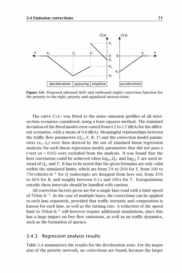
3.4 Emission corrections 71
x
C x( )C x( )
x
ea
0
ed
eq
ec
0
es
xaxsxqxd
accelerationstoplinequeuingdeceleration
Figure 3.6: Proposed inbound (left) and outbound (right) correction function forthe priority-to-the-right, priority and signalized intersections.
The curve C(x) was fitted to the noise emission profiles of all inter-
section scenarios considered, using a least squares method. The standard
deviation of the fitted model error varied from 0.2 to 1.7 dB(A) for the differ-
ent scenarios, with a mean of 0.6 dB(A). Meaningful relationships between
the traffic flow parameters (Qx , F , R, T ) and the correction model param-
eters (xi, ej) were then derived by the use of standard linear regression
analysis; for each linear regression model, parameters that did not pass a
t-test (α = 0.05) were excluded from the analysis. It was found that the
best correlation could be achieved when log10Qx and log10 T are used in-
stead ofQx and T . It has to be noted that the given formulas are only valid
within the simulated limits, which are from 5 % to 20 % for F , from 100 to
750 vehicles·h−1 for Q (subscripts are dropped from here on), from 20 %
to 40 % for R, and roughly between 0.1 s and 100 s for T . Extrapolations
outside these intervals should be handled with caution.
All correction factors given are for a single lane road with a limit speed
of 70 km·h−1. In the case of multiple lanes, the corrections can be applied
to each lane separately, provided that traffic intensity and composition is
known for each lane, as well as the turning rate. A reduction of the speed
limit to 50 km·h−1 will however require additional simulations, since this
has a large impact on free flow emissions, as well as on traffic dynamics,
such as the formation of queues.
3.4.3 Regression analysis results
Table 3.4 summarizes the results for the deceleration zone. For the major
arm of the priority network, no corrections are found, because the larger

72 Corrections on the Noise Emission near Intersections
part of the vehicles does not accelerate nor decelerate on this arm; traffic
on this arm has priority. No significant difference was found between the
major and the minor arms of the priority-to-the-right and the signalized in-
tersections. A positive correlation with the extra travel time log10 T and/or
the traffic intensity log10Q was found for xd as well as for ed. E.g. for the
priority-to-the-right intersection, the following relationships were found:
xd = 167.8 log10 T (3.12)
ed = −9.8+ 5.4 log10 T (3.13)
In this case, the longer the delay or the queue at the intersection, the larger
the distance at which a correction should be applied, but the less the actual
reduction in sound emission. Obviously T has to be >1 s to result in a
positive xd; however, T was found to be at least 3 s in the priority-to-the-
right intersection.
For the queuing area, no significant differences were found between the
different types of intersections, but a classification based on the extra travel
time was made; correction coefficients are shown in Table 3.5. A queuing
area only exists when log10 T > 1.4, as already mentioned in Section 3.3.1;
otherwise xq can be chosen at the stopline xs . Only log10 T was found to
be a significant predictor for the queuing area correction. The fraction of
heavy vehicles F (in %) also had some influence on xq (heavy vehicles are
also longer), but this was not statistically significant (p = 0.066).
Noise emission corrections at the stopline (es ) are mainly influenced by
the extra travel time associated with the inbound arm and by the fraction of
heavy vehicles, as summarized in Table 3.6. The correction starts slightly
negative for low values of T and F . A larger average extra travel time
is caused by vehicles slowing down when arriving at the intersection. The
subsequent acceleration near the stopline then results in a higher es , which
can eventually rise to 7 dB(A) for high traffic intensities. As can be expected,
the correction is smaller for the signalized intersection, because a large part
of the traffic here can cross the intersection without stopping. Again, no
correction is found for the major priority arms of priority junctions.
For the priority-to-the-right intersection, it was found that the correc-
tions at the center (ec) could best be described by a subdivision based on
log10 T , analogous to the queuing correction; for higher T the correction
becomes smaller. A small center correction ec for the major arm of the pri-
ority network was found, mainly correlated to the percentage R of traffic
turning left or right.
Finally, results for the acceleration area are given in Table 3.7. For all
intersection types, the amount of heavy traffic has the largest influence
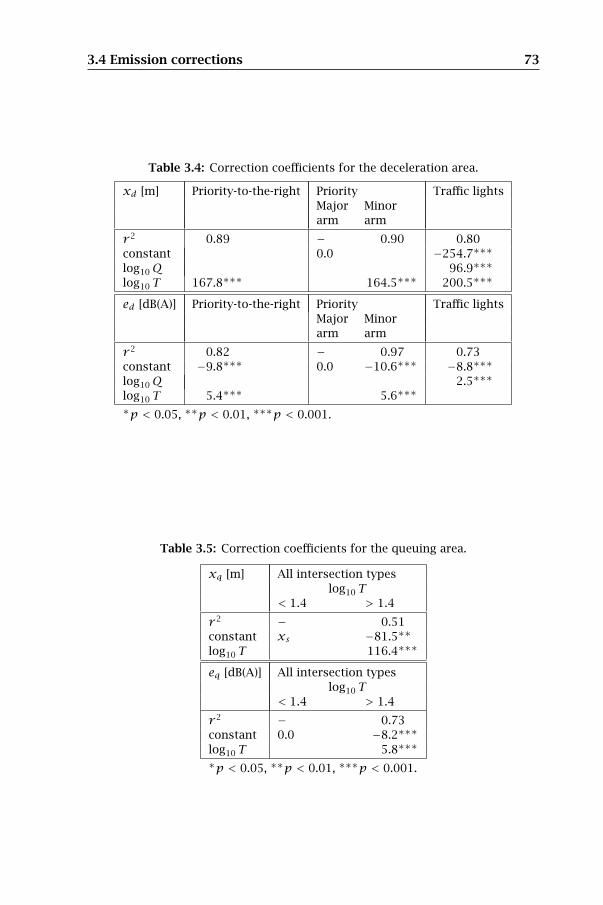
3.4 Emission corrections 73
Table 3.4: Correction coefficients for the deceleration area.
xd [m] Priority-to-the-right Priority Traffic lightsMajor Minorarm arm
r 2 0.89 − 0.90 0.80constant 0.0 −254.7∗∗∗
log10Q 96.9∗∗∗
log10 T 167.8∗∗∗ 164.5∗∗∗ 200.5∗∗∗
ed [dB(A)] Priority-to-the-right Priority Traffic lightsMajor Minorarm arm
r 2 0.82 − 0.97 0.73constant −9.8∗∗∗ 0.0 −10.6∗∗∗ −8.8∗∗∗
log10Q 2.5∗∗∗
log10 T 5.4∗∗∗ 5.6∗∗∗
∗p < 0.05, ∗∗p < 0.01, ∗∗∗p < 0.001.
Table 3.5: Correction coefficients for the queuing area.
xq [m] All intersection typeslog10 T
< 1.4 > 1.4
r 2 − 0.51constant xs −81.5∗∗
log10 T 116.4∗∗∗
eq [dB(A)] All intersection typeslog10 T
< 1.4 > 1.4
r 2 − 0.73constant 0.0 −8.2∗∗∗
log10 T 5.8∗∗∗
∗p < 0.05, ∗∗p < 0.01, ∗∗∗p < 0.001.

74 Corrections on the Noise Emission near Intersections
Table 3.6: Correction coefficients for the stopline area.
es [dB(A)] Priority-to-the-right Priority Traffic lightsMajor Minorarm arm
r 2 0.90 − 0.91 0.53constant −3.1∗∗∗ 0.0 −3.4∗∗∗ −1.8∗∗∗
log10 T 4.3∗∗∗ 5.3∗∗∗ 3.2∗∗∗
F 0.06∗∗ 0.06∗∗
ec [dB(A)] Priority-to-the-right Priority Traffic lightslog10 T Major Minor Major Minor
< 1.4 > 1.4 arm arm arm arm
r 2 0.60 0.50 0.73 0.66 0.64 0.41constant 12.0∗∗∗ −5.5∗∗∗ 1.8∗ 10.0∗∗∗ −4.8∗∗∗ −3.4∗∗∗
log10Q −7.7∗∗∗ −0.73∗∗ −5.1∗∗∗
log10 T 2.7∗∗ 1.7∗∗ 1.6∗∗∗ 2.1∗∗∗ 1.4∗∗∗
R −0.06∗∗∗ −0.04∗∗
∗p < 0.05, ∗∗p < 0.01, ∗∗∗p < 0.001.
Table 3.7: Correction coefficients for the acceleration area. For ea, the averageand standard deviation are given.
xa [m] Priority-to-the-right Priority Traffic lightsMajor Minorarm arm
r 2 0.81 − 0.50 0.65constant −35.0∗∗∗ 0.0 47.1∗∗∗ 33.7∗∗∗
log10Q 33.5∗∗∗
F 2.0∗∗∗ 1.8∗∗∗ 1.0∗∗∗
R −0.54∗
ea [dB(A)] Priority-to-the-right Priority Traffic lightsMajor Minorarm arm
constant −1.81 ± 0.20 0.0 −2.28 ± 0.61 −2.41 ± 0.42∗p < 0.05, ∗∗p < 0.01, ∗∗∗p < 0.001.
3.5 Discussion and conclusions 75
on the length xa of the acceleration area, because the maximum acceler-
ation for heavy traffic is lower. For the priority-to-the-right junction, it is
found that also the traffic volume makes the acceleration after a junction
more slowly; vehicles are more interrupted at the crossing when the traf-
fic volume increases. Note that the traffic volume on the outbound lane is
influenced by both the traffic volume on the minor and the major inbound
arms. On the minor outbound arm of the priority junction, the length of
the acceleration area is to a small extent also influenced by the amount
of vehicles that enters this lane from the major arm (turning rate R). For
the signalized intersection, the influence of the heavy traffic percentage
becomes smaller, because during the greentime on the major arm (which
is most of the time), vehicles do not have to decelerate at the crossing.
No significant correlations were found for ea, but the variations in this co-
efficient were small, so the average is given in Table 3.7. In all cases, a
negative ea was found; positive values (corresponing to higher levels due
to acceleration) may be possible if the speed limit on the outbound lane is
lower.
3.5 Discussion and conclusions
Current traffic noise prediction models, which are mostly based on macro-
scopic traffic simulation, do not allow to study the influence of traffic dy-
namics near junctions on local noise levels. The goal of this research was
to prove that it is possible to refine noise calculations based on the output
of these models in the neighbourhood of intersections, using a correction
on the average vehicle emission, aggregated in lane segments. For this, a
case study consisting of the microsimulation of a large set of intersection
scenarios was conducted. The intersection type was found to have a sig-
nificant influence on travel times. Global noise emission of the different
intersection types was compared to the situation in which the presence of
an intersection is neglected when calculating noise emissions. It was found
that, in the non-congested state, the variation in total noise emission be-
tween different intersection types becomes lower than 1 dB(A) when one
aggregates over segments with a length of 140 to 340 m, depending on the
traffic demand and composition. Noise immission calculations for the in-
tersection scenarios were compared to some previous measurement results
found in literature, and in general a good agreement was found.
However, there were large spatial differences in noise emission. The re-
sults indicated that a spatial approach should be used; deceleration, queu-
ing, stopline and acceleration zones were observed. A correction model,

76 Corrections on the Noise Emission near Intersections
based on a piecewise linear approximation of the average noise emission
by all vehicles in each lane segment close to the intersection, was proposed.
Finally, it was shown that meaningful relationships can be derived between
the proposed noise emission corrections and traffic flow parameters. The
results obtained in this chapter are only applicable for the range of traffic
situations studied. The methodology can however easily be used to study
typical intersections for a region and to extrapolate the results to the whole
network under study.

Part IIMusic in the Temporal
Structure of Soundscapes


Chapter4
Methodology and
Mathematical Background
In this chapter, we will construct a novel indicator for the structure
of the temporal envelope of environmental soundscapes. The main
concepts will be introduced, together with the necessary mathematical
background; further references will be given for the interested reader.
In the following chapters, some partial aspects will be explained more
in depth.
4.1 Time-frequency analysis of stochastic signals
In essence, the temporal envelope of a sound fragment can be regarded as
a stochastic signal. Random or stochastic signals are by definition unpre-
dictable, and are thus often analyzed and characterized in statistical terms.
In this section, we will introduce the most basic concepts for such a statis-
tical analysis in relatively intuitive terms; for a more rigorous discussion
we refer to [7] or [186].
4.1.1 Stationarity
Often, it is required that the stochastic signal under study is stationary,
which means that its statistical properties (i.e. its probability distribution)
are independent of time. A weaker form, called second-order stationarity,
only requires that the 1st and 2nd moments (i.e. the mean and variance)
do not vary with respect to time.
It must be mentioned that the temporal envelope of environmental
sound is most often not stationary. For example, we may consider the
case of road traffic noise. The temporal envelope of the sound of a single

80 Methodology and Mathematical Background
car passing by is obviously not stationary. Measurements during a whole
day will be affected by variations in traffic intensity related to the period of
the day (e.g. night time vs. rush hour), resulting in a time-dependent mean
and variance. However, if the measurement or simulation duration is cho-
sen carefully, the temporal envelope may be stationary. The duration of
the fragment should be long enough to include several passages; the no-
tion of a “sufficiently long period of time” depends on the traffic intensity.
For average to high traffic intensity, several minutes may be sufficient (we
refer for example to Figure 2.4); for low traffic intensity longer periods
are necessary. The requirement of not including substantial variations in
traffic intensity fixes the upper limit of the duration. In this work, often
a recording/simulation duration of 15 minutes or 1 hour is considered,
which suffices in most cases.
4.1.2 Time correlations and spectral density
Let X(t) be a stationary stochastic signal, e.g. the temporal envelope (in-
stantaneous power, loudness, pitch…) of a sound fragment. For simplicity
we assume that the duration of this fragment is infinite. The (linear) aver-
age value of X(t) is given by
〈X(t)〉 = limT→∞
1
T
∫ T0X(t)dt (4.1)
We may define the function X′(t) = X(t) − 〈X(t)〉, for which the average
value is zero. Since we are mainly interested in the temporal structure of
X(t), we shift our focus to X′(t); the average 〈X(t)〉 is accounted for by
measures such as LAeq, average loudness etc.; accents are dropped from
here on.
The autocorrelation function C(τ) is a quantitative measure of how the
fluctuations in X(t) are correlated between times t and t + τ :
C(τ) =
∫∞0X(t)X(t + τ)dt (4.2)
The autocorrelationC(τ) is useful for finding repeating patterns in a signal.
For example, when a recurring sound event results in a peak in the temporal
envelope at about each 10 s, C(τ) will show peaks at 10 s, 20 s, 30 s etc.
Although C(τ) already gives a complete description of the temporal
structure of X(t), it is often more convenient to work in the frequency
domain instead of the time domain. The strength of the fluctuations of
X(t) is described by its variance 〈X2(t)〉. The spectral density SX(f ) (also
called the power spectrum) is defined as the variance of X(t) in a unit of

4.1 Time-frequency analysis of stochastic signals 81
bandwidth centered around f . SX(f ) may be measured by passing X(t)
through a band-pass filter with central frequency f and bandwidth ∆f . If
we call the resulting signal X∆f (t), then we have
SX(f ) ≡ lim∆f→0
〈X2∆f (t)〉
∆f(4.3)
Repeating patterns in X(t) will show up in the spectral density as single
peaks, e.g. the recurring event at about each 10 s will result in a peak at
about 0.1 Hz.
According to Parseval’s theorem (see e.g. [7]), the spectral density SX(f )
can be calculated analytically as the square of the Fourier spectrum:
SX(f ) =
∣∣∣∣∫∞
0X(t)e−2πift dt
∣∣∣∣2
=∣∣F[X](f)
∣∣2(4.4)
If X(t) is approximated by a discrete signalXn withn ≥ 0 (e.g. a time series
of LAeq,1s values), its spectral density can be estimated by use of the discrete
fourier transform (dft). The fast fourier transform (fft) is a commonly
used optimal implementation. An implementation of the calculation of
SX(f ) for a discrete signal will be given in Appendix A. Furthermore, SX(f )
and C(τ) are not independent, but are related by the Wiener-Khintchine
theorem [7]
SX(f ) =
∫∞0C(τ) cos(2πfτ)dτ (4.5)
4.1.3 Types of stochastic signals
Many stochastic signals may be characterized by a single correlation time
τc . In such a case, X(t) and X(t + τ) are correlated for τ ≪ τc and inde-
pendent for τ ≫ τc . Usually, the autocorrelation function is of the form
C(τ) = A exp(−τ/τc). Using Eq. 4.5, one can easily calculate the spectral
density as
SX(f ) =Aτc
1+ 4π2f 2τ2c
(4.6)
One can see that SX(f ) is independent of f in the frequency range corre-
sponding to periods over which X(t) is independent (f ≪ 1/2πτc), and
is a rapidly decreasing function of f , usually 1/f 2, in the frequency range
over which X(t) is strongly correlated (f ≫ 1/2πτc). More in general, a
steep slope of SX(f ) indicates a strong temporal correlation, while a flat
slope indicates a weak temporal correlation.
A special case occurs when SX(f ) ∼ fα, which results in a straight line
when plotted on a log-log chart. A stochastic signal with a flat spectral

82 Methodology and Mathematical Background
(e)
(d)
(c)
(b)
(a)
Figure 4.1: Samples of stochastic signals: (a) white noise, (b) 1/f noise, (c) 1/f 2
noise, (d) instantaneous power level of an excerpt of the 1st Brandenburg Concertoby J. S. Bach and (e) time series of LAeq,1s measured in a shopping street in Ghent.
density (slope α = 0) is called white noise: no correlation exists at all, and
the autocorrelation function is proportional to the Dirac delta function.
This is of course an idealized description, as frequency integration over
a constant SX(f ) would result in an infinite variance 〈X2(t)〉. Practical
stochastic signals are thus never truly white, as their spectral density will
only be relatively constant up to a certain cutoff frequency. A stochastic
signal for which SX(f ) ∼ 1/f 2 is often referred to as 1/f 2 noise or brown
noise. Plotted on a log-log scale, SX(f ) will be a straight line with a slope
α = −2. The intermediate case is called 1/f noise or pink noise. Figure 4.1
shows some examples of stochastic signals.
From this discussion it is clear that a stochastic signal with a 1/f spec-
tral density cannot be characterized by a single correlation time. In fact,
the 1/f spectral density implies some correlation in X(t) over all periods
corresponding to the frequency range for which SX(f ) ∼ 1/f . In [146], it is
proven that in the case of 1/f noise, C(τ) ∼ − ln(τ). Another interesting
property of 1/f noise is the fact that the signal power is equally divided
between each frequency decade, i.e. the integral
∫ 10f
fSX(f
′)df ′ ∼
∫ 10f
f
1
f ′df ′ =
∫ 10f
fd lnf ′ = ln 10 (4.7)
is independent of f .

4.1 Time-frequency analysis of stochastic signals 83
4.1.4 1/f noise in nature and music
While white and 1/f 2 noise are mathematically and physically well under-
stood, they are characteristic to only a relatively small number of natural
fluctuating phenomena. A wealth of natural “signals” show a 1/f spectral
density, often in a wide frequency range; an overview can be found in [260]
and [333]. The oldest and maybe most famous example is the flicker noise
in vacuum tubes, for the first time measured by Johnson [165]. Other fa-
mous examples are the fluctuations in the strength of the light originating
from quasars [184], the flow rate of numerous rivers [209, 188] and the
Gutenberg-Richter law for the magnitude of earthquakes [131].
An interesting and totally unexpected occurence of 1/f noise was found
by Voss and Clarke [328, 329] in the temporal envelope of music and
speech. To estimate the temporal envelope of the amplitude of audio
broadcast signals, they squared the audio signal and filtered the result
with a low-pass filter, to obtain a signal that varies with the loudness of the
audio signal. They found that the spectral density of this temporal enve-
lope showed a remarkable good resemblance to 1/f , for all radio stations
investigated, spanning several musical genres. Next to this, they estimated
the instantaneous pitch as the rate of zero crossings of the audio signal;
again, a good agreement with 1/f was found for the spectral density of
instantaneous pitch. A decade later Hsu et al. [149, 148] proved, by analyz-
ing musical scores, that this 1/f is inherent to the music itself, and not a
result of its performance and recording, since it can be traced back to the
sequence of intervals between successive notes.
Furthermore, Voss and Clarke found that artificial music with 1/f char-
acteristics was perceived the most pleasant by a panel of listeners [329].
A flatter slope (α = 0) resulted in too chaotic music, while a steeper slope
(α = −2) resulted in too boring music. Music certainly does have a structure
on all different timescales. It thus appears that these scales are distributed
roughly logarithmically in time and have comparable amplitude variations
at each level of structure. For example, there are four notes to a phrase,
four phrases to a bar, three bars to a theme, three repetitions of a theme in
a development, three developments in a movement, three movements in a
concerto, and perhaps three or four concertos in a radio broadcast [260].
We have to note that the claim for the existence of 1/f in music by
Voss and Clarke has been criticized by musicologists. Nettheim [232] ar-
guments that from a musical point of view, the instantaneous pitch, as
defined in [329], considers both rhythm (duration of notes), as well as
pitch (frequency of notes). To consider pitch and rhythm independently,
one has to depart from the score, rather than from a recording. Further-
more, Nettheim criticizes the validity of the procedure of Voss and Clarke,

84 Methodology and Mathematical Background
in which long duration stretches of radio broadcast are used, including
various pieces from different composers and styles, as well as spoken an-
nouncements and comments. He emphasizes that “a single piece is nor-
mally the largest unit of artistic significance” [232]. Using a large data set
of (classical) musical pieces, Nettheim found that the spectral density for
pitch tended more towards 1/f 2, for periods up to about four bars of busic.
In a similar way, Boon and Decroly [33] and Boon and Prigogine [34] found
power spectra fα with α between −1.79 and −1.97 in the frequency range
[0.03 Hz, 3 Hz]. Boon and Decroly acknowledge that long time sequences
yield a 1/f spectrum. However, they also stress that the meaning of long
stretches of blended musical pieces is unclear.
When environmental soundscapes are the object of study, it is obvi-
ous that only physical recordings can be considered, as there exists no
soundscape “score”. Only the analysis methodology as proposed in [329]
is therefore applicable to environmental soundscapes. As we also will show
in Chapter 5, this methodology usually results in a 1/f spectral density for
music, for single pieces as well as for longer recordings consisting of mul-
tiple pieces. Furthermore, although the slope of the spectral density is a
point of debate, a straight line spectral density, which is typical for a com-
plex system, is almost always found, irrespective of the analysis method-
ology. Finally, most criticism addresses the claim of 1/f in the frequency
fluctuations of music, rather than in the loudness fluctuations, which are
considered in this work.
In Chapter 5, we will further discuss this topic, and we will show that
a 1/f spectral density is characteristic not only for music, but also for the
temporal envelope of various rural and urban soundscapes.
4.2 Fractal analysis of stochastic signals
Another approach is to consider stochastic signals as fractals. This term
was introduced by Mandelbrot [208] to describe geometric objects that have
a fine structure, are recursively self-similar (parts are exactly or approxi-
mately similar to the whole object) in an exact or a stochastic way, and re-
semble shapes found in nature. A classical example is the coastline curve of
Britain [207]. When looked at it from high altitude, the coastline is formed
by bays and peninsulas. However, when one takes a closer look, these bays
and peninsulas are itself formed by smaller bays and peninsulas, and so
on.
As a consequence, the measured length of a stretch of coastline seems
to depend on the size of the ruler used. The smaller the ruler, the longer

4.2 Fractal analysis of stochastic signals 85
the measured length becomes, as a smaller ruler will be laid along a more
curvilinear route. The empirical evidence suggests a relationship which, if
extrapolated, shows that the measured length L(r) increases without limit
as the ruler length r decreases towards zero [207]:
L(r) ≈ Ar 1−D (4.8)
The value of the exponent D seems to depend on the coastline (e.g. 1.25
for the West Coast of Britain and 1.02 for the coastline of South Africa).
This exponent was interpreted by Mandelbrot as a fractional dimension
(hence the term fractal), because it corresponds closely to the definition
of the Hausdorff dimension, a generalized definition of dimension used in
topology.
In [133], the fractal properties of the horizon were studied for various
kinds of landscapes. Using an experiment involving a panel of testpersons,
a relation between the fractal dimension of the horizon and landscape aes-
thetic preference was found. In this section, we will show that the fractal
dimension of stochastic signals is strongly related to their spectral density.
4.2.1 Box-counting dimension
We will not go into detail on the theory of fractal geometry (a thorough
mathematical treatment can be found in [95]). Rather, we will outline a
method to estimate the fractal dimension of a stochastic signal. A number
of different definitions for the dimension of a curve exist; for most well
behaving fractals these all result in the same value. The Minkowski dimen-
sion or box-counting dimension [95, 283] is the most widely used, since it
is relatively easy to compute.
Let X(t) again be a (continuous) stochastic signal. It may be proven
that if the first derivative of X(t) is continuous, the curve will have a di-
mension of 1, just like a simple straight line [95]. However, when X(t)
is sufficiently irregular, its graph may have a dimension larger than 1, i.e.
locally plane filling. The best known mathematical example may be the
Weierstrass function
Xw(t) =∞∑
k=1
λ(s−2)k sin(λkt
)(4.9)
with 1 < s < 2 and λ > 1. This function is continuous but nowhere deriv-
able; it can be proven that the fractal dimension of this function equals
s [95].

86 Methodology and Mathematical Background
X(t)
t
δ
Figure 4.2: Calculation of the box-counting dimension.
In Figure 4.2, the graph of an example stochastic signal is drawn in the
(t,X(t)) plane. Let us divide the abscissa into segments with length δ. We
may cover the graph with squares with side δ, joined up tightly, as shown
on the figure. Let Nnδ be the number of squares needed to cover the part
of X(t) in the nth segment. The total number of squares needed to cover
the graph up to a duration T will then equal
Mδ =T/δ∑
n=1
Nnδ (4.10)
If for δ→ 0 the relationship
Mδ ≈ cδ−D (4.11)
is observed with c a positive constant, then the fractal dimension of (the
graph of) X(t) equals D by definition, given by
D = − limδ→0
log10Mδ
log10 δ(4.12)
4.2.2 Relation with spectral density
For (mathematical) signals with a spectral density SX(f ) ∼ fα for f ranging
from f0 > 0 to ∞, it can be proven (see [95, 68]) that
D =5+α
2(4.13)

4.3 Complex systems 87
This relationship is only valid for α < −1. To see this, we note that the
energy E of the signal X(t) is proportional to the area below the spectral
density curve:
E ∼
∫∞f0
SX(f )df ∼
∫∞f0
fα df (4.14)
For α < −1, it may easily be proven that E is finite. If α → −1 (1/f
noise), the energy in the signal will increase to infinity (the energy in each
frequency decade is the same) and the fractal dimension will approach 2.
When α ≤ −3, X(t) looses its fractal properties (D = 1).
Physical signals always contain a finite amount of energy, and their spec-
tral density will not contain any frequency components above some cutoff
frequency. Therefore,D will always be 1 in a mathematical sense — the fine
structure will always disappear when one looks close enough. However, it
is often the case that α ≈ −1 within a frequency interval [f1, f2]. Eq. 4.13
will then provide an overestimate of D. In this work, we will nevertheless
apply Eq. 4.13 for frequency intervals in a pragmatic sense.
4.3 Complex systems
4.3.1 Self-organized criticality
Complex systems, which may informally be described as systems of many
parts which are locally coupled in a nonlinear fashion [353], are the ori-
gin of most stochastic time series found in nature. It seems obvious to
expect a common principle which explains the omnipresence of 1/f noise
in natural complex systems. However, until now no universally accepted
explanation exists; most of the theories are only applicable to one system.
In 1987, Bak et al. [8] introduced the notion of self-organized criticality
(soc), which is now considered as one of the best candidates to explain
1/f characteristics in many physical systems.
Self-organization
Self-orginization (so) is the process in which the internal order of a sys-
tem is increased without being guided by an outside source [235]. A more
concrete definition can be found in [53]: “A process in which a pattern at
the global level of a system emerges solely from numerous local interac-
tions among the lower-level components of the system”. The appearance
of so was first noted in the physical fields of phase transitions and crys-
tal growth. Self-organization requires a complex system not in thermody-
namic equilibrium, and in which nonlinear feedback relations are present.

88 Methodology and Mathematical Background
Positive feedback is necessary for the amplification of random fluctuations,
to drive the system into an ordered state, distinguishable from the random
configuration of thermodynamic equilibrium. Some negative feedback to
dampen the effects of random fluctuations is also necessary, in order to be
able to maintain the ordered state. A system fulfilling these conditions may
evolve to one of many possible new states, which can be highly organized.
Self-organization often leads to the emergence of complex patterns,
which are unpredictable from the lower level elements of the system. Clas-
sical examples are the human brain, capable of thought, as a cause of the
interactions between numerous neurons [173], or the formation of a ter-
mite hill. Self-organization has been used to describe the formation of
complex patterns and behaviour in many fields of science such as neuro-
science, biology, ecology, sociology and economics — an overview can be
found in [287] and [53].
Critical point in phase transitions
As it is well known from thermodynamics, in systems containing matter
in liquid and gaseous states, there exists a special combination of pres-
sure and temperature, known as the critical point [180]. Under these con-
ditions, the transition between liquid and gas becomes a continuous or
second-order transition, with which no latent heat is associated. Near the
critical point, the distinction between liquid and gaseous phase is almost
non-existent. Normally transparent liquids may appear milky; this phe-
nomenon is called critical opalescence (see e.g. [241]). It is explained by
the random density fluctuations on a microscopic scale. Small volumes of
liquid fluctuate constantly into a gaseous state and back again, since al-
most no energy is needed for this. As the critical point is approached, the
length scale at which the fluctuations occur grows, and at the critical point,
fluctuations will occur at all length scales (implying a fα spectral density).
If there is a difference in refractive index between both states, light will be
strongly scattered.
Self-organized criticality
This scale invariant phenomenon at the critical point in phase transitions
inspired Bak et al. to introduce the concept of self-organized criticality.
Systems showing soc will after a long enough time evolve to a macro-
scopic state called an attractor, which shows the scale invariance found
at the critical point in second-order phase transitions. Crucial is the fact
that the complexity in the model introduced in [8] emerges in a robust (i.e.

4.3 Complex systems 89
self-organized) manner, which does not depend on fine-tuning of parame-
ters, as it is the case with the critical point in phase transitions. soc can be
considered as a mechanism by which complexity can emerge from simple
local interactions in a spontaneous fashion, rather than in a way only pos-
sible in the lab with control parameters tuned to precise values. Therefore,
soc is plausible as a source of natural 1/f characteristics.
The concept of soc was illustrated in [8] by a dynamic system resem-
bling a pile of sand. Consider a flat square surface on which a large pile of
sand is put. If the slope at some point on the pile is too large (larger than
a critical value), the pile is not in equilibrium and it will collapse at that
point, resulting in an avalanche. The sand pile system will evolve until a
state at the edge of stability is reached, at which the average slope is near
the critical value. Random perturbations (dropping a single grain on a ran-
dom location) will then result in avalanches on all length scales: they may
have no effect, but they may also cause a cascading reaction that effects
every site on the pile. There are no parameters in this system, since a shift
in critical value will simply shift the pile of sand, and fixed boundaries are
used, since the height of the pile of sand has to be zero at the edges of the
surface.
The notion of soc still receives wide attention from researchers in vari-
ous fields, ranging from plasma physics over neuroscience to ecology. The
initial sand pile model by Bak et al. was extended by many (we men-
tion [66, 76, 211]) to be able to explain a 1/f spectral density in a wide
frequency range. Many other models were proposed as examples of soc,
such as the forest fire model and the earthquake model — a review can
be found in [58]. Some questions still remain unanswered, e.g. to date,
there is no known set of general characteristics that guarantee a system
will display soc.
4.3.2 Road traffic as a complex system
An overview of some complex systems that may influence natural, rural and
urban soundscapes will be given in the next chapter. One complex system
of particular interest in this work is road traffic. Vehicles may be consid-
ered as “locally coupled” since each driver can only see a restricted num-
ber of vehicles in front. Smaller and larger groups of vehicles are formed
as a consequence of human driving behaviour and the natural spread in
vehicle speed and acceleration. Already some decades ago [226], fluctua-
tions with a 1/f spectral density were found in the flow rate of (highway)
traffic near saturation. Microscopic traffic flow models based on cellular
automata (see Section 1.2.2) were since then succesfully used to model

90 Methodology and Mathematical Background
this behaviour [305, 350, 55], and soc was found to be a possible expla-
nation [228, 250, 227]. In Section 5.2.3, the possible influence of 1/f road
traffic flow characteristics on urban and rural soundscapes will be further
investigated.
Furthermore, it was found that the presence of both signalized [57] and
non-signalized [231] intersections, as well as the presence of sidestreets
[230], catalyzes the emergence of soc and 1/f fluctuations. As a con-
sequence, even if traffic is loaded at the edges of the network randomly
distributed in time, 1/f fluctuations may occur in urban traffic networks
without having to model a large area around the study area. This con-
trasts to the case of highway traffic, where a long stretch of road has to be
simulated to obtain a realistic spatial and temporal vehicle distribution.
4.4 Music-likeness as a fuzzy indicator
So far, we have learned that the spectral density of the temporal envelope of
music often displays a 1/f structure. As will be shown in the next chapter,
this is also the case with various natural, rural and urban soundscapes.
1/f characteristics were found to be ubiquitous in nature; an explanation
based on self-organization of the underlying complex systems was given.
Futhermore, the link between the slope of the spectral density and the
fractal dimension of a stochastic signal was discussed.
Two links with perception were found: the slope of the spectral den-
sity seemed a good indicator for the pleasantness of artificial music, and
the fractal dimension of the horizon was found to be a good indicator for
landscape aesthetics. In our opinion, these arguments suffice to introduce
an indicator for the temporal structure of soundscapes, based on the sim-
ilarity with the temporal structure of music. We will call this indicator the
music-likeness.
It was pointed out that a 1/f spectral density can only be observed in a
finite frequency interval for physical signals. In the next chapter, it will be
shown that often a breaking point around 0.2 Hz is found in the slope of
the spectral density of many rural and urban soundscapes. Two frequency
intervals are of interest: the first one from 0.002 Hz to 0.2 Hz, correspond-
ing to periods of 5 s to 10 minutes, and the second one from from 0.2 Hz
to 5 Hz, corresponding to shorter time scales. A naïve implementation of
our novel indicator would simply fit a straight line through SX(f ) (plotted
on a log-log scale) in the frequency interval of interest, calculate the slope
4.4 Music-likeness as a fuzzy indicator 91
α, and measure the difference in slope with the case of α = −1 as
1− |1+α| (4.15)
However, one has to consider the fuzziness in the statement “similar to
the temporal structure of music” carefully. As the numerous graphs in the
next chapter illustrate, the resemblance to a 1/f spectrum is never exact,
neither for music nor for general soundscapes. The spectrum will never be
a straight line in a mathematical sense, and the slope of the best fitting line
will never be exactly −1. A fanciful spectral density may result in a slope
of about −1, but due to the numerous peaks, the temporal structure may
not be music-like at all. Therefore, also the deviation from a straight line
ǫ has to be taken into account.
To account for this fuzziness, fuzzy set theory could be applied. We
will introduce the basic notions of fuzzy set theory and fuzzy logic briefly,
in order for the reader to be able to understand the construction of the
music-likeness indicator, introduced in Chapter 6. For a more thorough
discussion, we refer to [88].
4.4.1 Fuzzy sets
In classical set theory, a characteristic function is associated with each set,
which yields the value 0 or 1 for each element of the universe of discourse
U , indicating whether the argument belongs to the set or not. This is a
crisp condition; fuzzy set theory generalizes the concept of set member-
ship by extending the range of the characteristic function from {0,1} to the
unit interval [0,1]. This extension allows a gradual transition from “not
belonging to a set” (0) to “belonging to a set” (1).
A fuzzy set A on a universe of discourse U is fully characterized by its
membership function µA : U → [0,1], where µA(u) denotes the member-
ship degree to which u ∈ U belongs to A. The collection of all fuzzy sets
on a universe of discourse U is denoted as F(U). When the universe of
discourse U has a finite number of elements, the fuzzy set A can be speci-
fied by a list of (membership degree, set element) pairs. If U has an infinite
number of elements, the membership function of A is usually given by a
functional representation.
In most practical cases, the universe of discourse U corresponds to the
collection of real numbers R. In literature, a number of commonly used
parametric shapes can be found [88]. The simplest membership functions
are formed using straight lines, such as the linear, triangular and trape-
zoidal functions. In this work, we will use the asymmetric Gaussian curve

92 Methodology and Mathematical Background
with ρ,σ1, σ2 ∈ R defined by
µ(.;ρ,σ1, σ2) : R→ [0,1]
u֏
exp(−(u−ρ)2
2σ21
)if u ≤ ρ
exp(−(u−ρ)2
2σ22
)if u > ρ
(4.16)
Some examples of asymmetric Gaussian membership functions are drawn
in Figure 6.2. The membership degree µA(u) can be interpreted as the
degree of similarity of the element u to the prototypical elements of A —
elements that fully belong to A [324].
4.4.2 Fuzzy operators
The classical operations on sets such as union, intersection and comple-
ment, can also be generalized to the notion of fuzzy sets. A natural re-
quirement of such fuzzy operators is that they have to coincide with their
crisp counterparts when they operate on classical, crisp sets. Obviously,
this extension is not unique but can be performed in various ways. The con-
cept of triangular norm (t-norm) and triangular conorm (t-conorm) [88] is
most often used as a generalization of intersection (conjunction) and union
(disjunction).
For our novel indicator, we want to express that the slope has to be more
or less−1, and that the deviation from a straight line has to be “small”; this
is an example of a logical conjunction. In this work, we will use the defini-
tion of Bandler and Kohout [88] for the t-norm T , which simply calculates
the product of both membership degrees:
T (., .) : [0,1]2 → [0,1]
µ1, µ2 ֏ µ1 · µ2(4.17)
The degree of music-likeness ml can then be calculated in the follow-
ing way. Let α and ǫ be the fitted slope and deviation from a straight line
of the spectral density of X(t). Let A and E be fuzzy sets on the uni-
verses of discourse Uα and Uǫ of slopes and deviations, characterized by
the membership functions µA and µE , and describing the typical slopes and
deviations found in music. The logical statement
α ∈ A and ǫ ∈ E (4.18)
is then evaluated by
µA(α) · µE(ǫ) (4.19)
4.4 Music-likeness as a fuzzy indicator 93
The membership functions µA and µE typical for music are derived in Chap-
ter 6. We refer to Appendix A for a formal calculation method of the degree
of music-likeness.
4.4.3 Fuzzy rules
Finally, it is possible to extend binary logic to the notion of fuzzy logic.
Instead of evaluating a logical proposition as either true (1) or false (0),
the truth function is extended to the interval [0,1]. Hence, truth also be-
comes a matter of degree. Fuzzy sets and fuzzy operators are the subjects
and verbs of fuzzy logic; fuzzy if-then rules are used to formulate the
conditional statements that comprise fuzzy logic. Interpreting an if-then
rule involves distinct parts: firstly evaluating the antecedent (applying any
necessary fuzzy operators) and secondly applying that result to the conse-
quent (i.e. implication). In the case of classical logic, if the premise is true,
then the conclusion is true. In the case of fuzzy logic, if the antecedent
is true to some degree, then the consequent is also true to the same de-
gree. Mathematically, the notion of logical implication can be extended to
the fuzzy case in a multitude of possible ways. Since we will not use fuzzy
logic in this work, we will not go into further detail, but instead refer to [88]
and [324].
Fuzzy rules are used in systems which apply approximate reasoning,
which often use linguistic terms to represent their state. The level of ab-
straction is hereby raised from reasoning with numbers to reasoning with
perceptions, more closely linked to the way humans reason in everyday life
situations.


Chapter5
1/f Noise in Rural and
Urban Soundscapes
B. De Coensel, D. Botteldooren and T. De Muer
Published in Acta Acustica united with Acustica 89(2):287–295, 2003.
« « «
In this chapter, the environmental soundscape is assumed to be the
voice of a complex system. It is shown that the spectral density of the
loudness and pitch temporal envelope of rural and urban soundscapes
quite often follows a 1/f frequency dependence. Furthermore, a link
with self-organized criticality is drawn. Results of this research were
presented at the 1st Pan-American/Iberian Meeting on Acoustics [38],
and a lay language version of this chapter was published online at the
ASA World Wide Press Room [37].
5.1 Introduction
A number of almost historical papers [328, 329] have studied the long-
term variations in level and pitch of different kinds of music that mankind
has produced. They made the surprising observation that all of the mu-
sical genres that were studied showed the same 1/f behaviour, both for
level and pitch variations. They also showed that artificial sound with these
characteristics was recognized as “music” by a listener. Music with a flatter
spectrum sounded too chaotic, too unpredictable. A steeper slope resulted
in too much predictability and hence boring and dull sound. Speech frag-
ments showed this 1/f behaviour to a lesser extent.

96 1/f Noise in Rural and Urban Soundscapes
These findings were so surprising that they have puzzled many. A lin-
ear dependence on a log-log scale emerges in the description of the dy-
namics of many complex systems [6]: the light from quasars, the intensity
of sunspots, the current through resistors, the flow of the Nile, a pile of
sand, stock exchange price indices, the use of words in English literature,
critical ecological systems, etc. In 1987, Bak et al. [8] introduced the notion
of self-organized criticality to explain 1/f noise. Although it is doubtful
that their initial model actually succeeded in predicting 1/f dynamics, self-
organized criticality (soc) is now generally believed as a source of linear
log-log behavior of complex systems [66, 76]. Therefore, in creating music,
man seems to imitate the temporal fluctuation of self-organized critical
systems, which are quite common in the (natural) living environment. In
Section 5.2, we include a more detailed discussion of complexity and self-
organized criticality.
Given the above observations it seemed obvious to look for 1/f -like
features in the dynamics of urban and rural soundscapes. Traditional re-
search on the impact of noise on the quality of the living environment and
human health has focused on indicators of average loudness as a primary
indicator. A-weighted sound pressure levels are often used as an approxi-
mate measure that is much cheaper to obtain. A vast amount of informa-
tion is now available on the relation between urban noise levels and major
impacts on the human observer such as reported annoyance and sleep dis-
turbance. However, designing an optimal urban soundscape involves much
more than just preventing annoyance, sleep disturbance, or negative health
impacts [325, 203, 20]. Several methodological procedures were proposed
to evaluate and categorize soundscapes (for an overview, see [284]). Based
on psychoacoustics and sound quality theory, the relation between envi-
ronmental sound and its perception can be clarified [118, 17]. In [267] the
authors make a strong attempt to link acoustic and psychoacoustic param-
eters to the subjective appraisal of urban sound.
Dynamics of the sound may be an important factor in this process. New
indicators are required to quantify this additional dimension. Percentile
psychoacoustic loudness was proposed for this purpose [267, 96], but this
neglects any cohesion between fluctuations in level. The 1/f behaviour
so common in music may be a good starting point for developing such
indicators. The fact that music and urban soundscapes have been linked
before [280] gives more confidence in the approach.
In this chapter we only observe soundscapes and indicate possible indi-
cators for cataloguing them based on their dynamics. It is not the purpose
of this chapter to link our observations to perception of the soundscape
by the human observer.
5.2 Complex systems & self-organized criticality 97
This chapter is organized as follows. In Section 5.2, complex systems
and self-organized criticality are discussed with special emphasis on the
mechanisms that may lead to 1/f behaviour in soundscapes. Section 5.3
briefly describes the methodology used to obtain and process the data.
Then, just to set the framework, a few music fragments are analyzed in
Section 5.4. Finally, rural and urban soundscapes are addressed in Sec-
tion 5.5.
5.2 Complex systems & self-organized criticality
This section investigates where self-organized criticality can be expected
in the urban and rural setting, and how this could theoretically lead to
observing 1/f noise in its soundscape. The term complexity is used to
describe a wide range of very different systems that have as a common
feature that their dynamic behaviour (or even their geometry) can not be
reduced to a single or small number of oscillators and time constants. No
general theory for treating complexity is widely accepted today. However,
it is clear that complexity emerges when a sufficient number of weakly in-
teracting systems form a “group” behaviour. As stated in the introduction,
many complex systems show a surprisingly linear relation in a log-log chart
for some of their characteristics, and self-organized criticality seems to be
able to explain this [66, 76]. Simulations of swarm dynamics and interact-
ing agents have shown that a common attractor combined with a closeness
factor that can be exchanged between particles or agents, together with
some damping are sufficient to create self-organized criticality [201].
Natural systems have been successfully described using the theory of
fractals [95]. Self-similarity, that is the discovery of very similar shapes
when zooming in or using a smaller ruler to measure, is an essential feature.
The fractal dimension D is introduced to describe how sizes change when
“zooming in”. For time series, the fractal dimensionD (as determined using
the box counting method) is related to the negative slope of the spectrum,
α, according to Eq. 4.13, if the fα trend extends over the whole spectrum
and α < −1. A fractal dimension D = 2 corresponds to 1/f dependence.
Brownian noise, another well-known dynamic, has D = 1.5 and shows a
1/f 2 dependence. White noise has α = 0 and D = 2.5. This brief discus-
sion on fractal dimension was introduced on behalf of those readers more
familiar with fractal theory and self-similarity than with complexity and
self-organized criticality. Both are clearly related, the former being more
descriptive, the latter being more explanatory. Let us now turn to the main
topic of this section, the identification of possible self-organized criticality
(soc) in the urban and rural setting that may influence soundscapes.
98 1/f Noise in Rural and Urban Soundscapes
5.2.1 Wind
It is well known that low frequency wind noise can contribute significantly
to outdoor noise measurements, especially in quiet areas. In [30] three
causes of wind noise are identified:
1. turbulence generated at the microphone membrane;
2. intrinsic turbulence in the air flow (pseudonoise), and
3. indirect sound caused by rustling grass, leafs, etc.
Since all soundscape recordings were done using adequate microphone
windscreens and at sufficiently low wind speeds, contribution (1) can be
neglected. In [222] Morgan et al. prove that for contribution (2) p = ρuv ,
where v is the average wind velocity, u is the rms value of the velocity fluc-
tuation and p is the rms value of the acoustic pressure. This is primarily a
low frequency contribution. When focussing on the frequency range that
contributes most to perception, secondary noise sources can easily be the
dominant source in terms of sound pressure level. Experimental data gath-
ered in open grassland [30] showed a relation LA95 = 22.6 log(v) + 22.7,
where v is the 5 minute average wind velocity. Wind induced noise in
trees was investigated in [101] both for a single tree and several forest
edges. For deciduous species (aspen, birch, oak) an average regression
LAeq ∼ 30 log(v) was found and for coniferous species LAeq ∼ 35 log(v)
seems to be a good trend. In these relations v is the average wind speed
(averaging time 10 seconds to 1 minute depending on the site) and LAeq is
the 10 second to 1 minute averaged A-weighted sound pressure level. It is
also shown in the same reference that the wind induced vegetation noise
spectrum does not change significantly with wind speed. In general, it can
be concluded that although wind induced sound pressure depends on the
degree of turbulence in the wind and on the vegetation that is present near
the observation point, it is on average proportional to vα. v is the average
wind speed and α is a coefficient somewhere between 1.1 and 2.
Let us now turn to long term variations (seconds to minutes) in the wind
speed. Turbulent flow is a typical example of a complex system showing
clear scaling laws. The flow in the atmospheric boundary layer is turbulent.
This turbulence is usually isotropic up to inhomogeneities of several meters
in size. Three models for locally homogeneous and isotropic turbulence are
commonly used in sound scattering studies: the Kolmogorov spectrum, the
Gaussian spectrum and the Von Karman spectrum [249]. For the purpose
of this evaluation, the Kolmogorov spectrum can most easily be used. It
predicts a −11/3 power law for the three-dimensional spectral densities
of random inhomogeneities in the inertial range. If it is further assumed

5.2 Complex systems & self-organized criticality 99
that these inhomogeneities are transported by the mean flow, a −11/9 or
approximate 1/f dependence of the local wind velocity fluctuation power
spectrum is obtained. Based on the relation between wind speed and wind
induced noise, 1/f dependence can be expected for the sound level power
spectrum of type (2) pseudo-noise, while this dependence approximates
1/f 2 more for wind induced vegetation sound level. The assumptions on
the temporal behaviour of wind that underlie these theoretical considera-
tions could not be backed up by experimental literature data. In particular,
no data were found on the time scales of importance for this work. There-
fore, wind velocity dynamics during recording will be verified explicitly in
Section 5.5.
5.2.2 Water
The dripping of water from a tab has often been used to illustrate how com-
plexity emerges at the border between order and chaos as the flow rate of
water increases. The log-log linear behaviour typical for self-organized sys-
tems has been observed in the flow of rivers. Therefore, it can be assumed
that the power spectrum of the sound level fluctuations of the sound ob-
served near running or falling water exhibits linear log-log behaviour as
well. An extensive literature search did not reveal the time scales on which
this may occur.
5.2.3 Road traffic
Highway traffic flow near saturation has long been recognized as a sys-
tem showing 1/f behaviour. Several models were proposed to explain this
characteristic [55, 350] and self-organized criticality (soc) has been pro-
posed as the mechanism. More recently the same dynamics were used for
inner city traffic in a Manhattan block road system [57]. Well below satu-
ration, the power spectral density of traffic flow intensity, Q, gets flatter,
approaching the limit of white noise.
To translate this dynamic behaviour to sound level fluctuations on a
time scale of a number of cars passing by, a few hypotheses are made. The
average sound intensity, I, observed at the edge of the road scales linearly
with traffic intensity, Q, if the dependence of sound power level on car
speed is neglected as well as the individual differences between cars. In
that case, the power spectral density of sound pressure level fluctuation
is expected to show 1/f behaviour. Since traffic bursts inevitably lead to
lower driving speed and this has a considerable impact on noise emission
at high speed, it is not expected that this relation is going to be exact.

100 1/f Noise in Rural and Urban Soundscapes
At very low traffic densities, events occur randomly. This results in a
long-term white noise characteristic for Q. The translation to noise levels
is however no longer as straight forward. The slow growing and falling of
the sound intensity of single cars passing by has to be taken into account.
If this intensity fluctuation for a single car passing by is approximated
by a Lorentz curve, the power spectrum will decay exponentially. On a
log-log plot this shows as a stronger than linear decay as a function of
frequency. The problem may however be obsolete since the soundscape
will be dominated by other sources in that case.
5.2.4 Bird song
Intensity of bird song in the rural and suburban soundscape varies con-
siderably during the day and strongly depends on the season. The dawn
chorus dominates the acoustics of the spring and summer early morning.
This burst of bird singing has attracted the attention of many animal be-
haviour scientists, but until today, no consensus is reached concerning its
origin. In [298], 12 hypotheses are described and evaluated with respect to
observed patterns: peak restricted to, and develops through the breeding
season; qualitatively different signals used during peak; diel pattern varies
among species. For the purpose of the research described in this work, it
is noted that a number of hypotheses indicate an optimum for each bird
individually independently of the presence and behaviour of individuals
of the same or a competing species. Recent research using stochastic dy-
namic programming [309] has given evidence in favour of the hypothesis
that regulation of fat reserves and time spent on foraging and singing are
related and can explain the increased song intensity at dawn, at least for
some species. Spending excess fat reserves at dawn and inefficient forag-
ing clearly result in an optimum that may occur at a slightly different mo-
ments for different species [310], but that is clearly the same for all birds
of the same species. Additional hypotheses such as better propagation of
acoustic signals, circadian cycles, and self-stimulation are at least partly
supported by the evidence [298] and also result in the same optimum for
all individuals of the same species.
Other hypotheses put forward for explaining the diel pattern of singing
involve interaction between various birds of the same species. They in-
clude [298] territory defense, mate guarding, mate stimulation, and general
social dynamics. These theories mention that dawn singing seems to be so-
cially contagious (i.e. the behaviour spreads from neighbour to neighbour),
at least for some species and to some extent. It is also obvious that simul-
taneous singing has a disadvantage due to masking and nobody listening.
5.3 Methodology 101
It has indeed been observed that males singing to defend their territory
stop singing occasionally during dawn bout to listen to their neighbours.
It has even been observed that species living in the same environment that
have similar songs, develop a non-overlapping diel pattern (i.e. they sing at
intermediate times).
The above discussion suggests that at least during dawn chorus singing,
the necessary ingredients are present to develop self-organized criticality:
there is a common optimal state for all individuals (enhanced by conta-
gious behaviour) and a repelling force that prevents them from acting too
similar. Moreover, in contrast to the mechanisms previously discussed,
dawn singing directly involves sound in the creation of soc. Therefore 1/f
dynamics of loudness and pitch fluctuation can be expected. It is not clear
how bird song during more quiet periods of the day is affected by these
mechanisms.
5.2.5 A mixture of urban activities
There is no clear evidence that the mixture of activities that determine
the soundscape of the inner urban shopping and recreating area has self-
organized criticality in it. However, at least some of the elements are
present. Each participant can be seen as an independent agent, each with
its private goal. To some extent, they strive to a common optimum. There
is some transfer of momentum leading to swarm-like behaviour and finally
there may be forces that repel at least some of the participants.
5.3 Methodology
Sound fragments of 15 minutes were used as basic material for this study.
These were recorded monaurally on dat tape using an omni-directional
microphone. For further processing, these samples were stored as 16 bit
pcm coded 44.1 kHz wav-files on computer disc. Since absolute amplitude
may get lost in the process, simultaneous sound level measurements using
standard equipment were performed during field recordings and later used
for calibration. Three types of pre-processing were applied:
(l) A-weighted level. Digital A-weighting filter followed by signal squar-
ing, 1st order digital Butterworth filter with cutoff frequency 20 Hz
(roughly corresponding to a 50 ms averaging time), and downsam-
pling by 200.
(n) Loudness. Loudness calculation is based on the model proposed by
Zwicker [352]. The implementation of the outer ear filter and 24 criti-

102 1/f Noise in Rural and Urban Soundscapes
cal bands follows the approximations proposed in [318]. Pre-masking
is neglected and a post-masking time constant of 100 ms is used.
Time integration is based on a low-pass filter and a time constant
of 40 ms as suggested in [352]. More accurate models for temporal
masking [257, 337] are available today and recent findings on per-
ceived loudness of fluctuating sounds may even indicate that avail-
able loudness models do not grasp the whole picture [127]. Although
these more accurate models should be included in future analyses, we
expect that this will not change any of the findings presented in this
chapter, where fluctuation over time intervals of more than 200 ms is
of primary interest.
(z) Instantaneous pitch. The signal is preconditioned by sending it
through a steep band-pass filter with cutoff frequencies 100 Hz and
10 kHz. The instantaneous pitch is approximated by counting the
number of zero transitions in 10 ms intervals similarly to the method
used in [329].
The A-weighted level was included to allow the analyses to be performed
on everyday sound level meters if required in future.
The power spectral density of loudness and pitch variations (notation
SL, SN and SZ) is obtained using the standard fft scheme, using a rectan-
gular time window of length 15 minutes. The choice of time window is
not very critical in this application. Finally, the curves obtained in the
log(amplitude) versus log(frequency) domain are locally averaged to 12
points per octave band.
5.4 Music and speech
For further comparison, the analyses of amplitude and pitch fluctuations
in music and speech presented in [329] are repeated using the software
modules described in Section 5.3. Figure 5.1 shows A-weighted level and
pitch fluctuations in 4 classical pieces. The duration of the fragments that
were analyzed varies between half an hour and one hour. The resemblance
to 1/f behaviour is obvious. Small deviations at the lower frequencies are
due to the finite duration of the sound samples. The flatter part below
10 Hz in “the 4 seasons” is caused by the fact that this music is composed
of shorter fragments, each taking 100 to 150 s.
Speech fragments behave slightly different (Figure 5.2). In the region
0.1 to 1 Hz the spectrum of pitch is almost flat, indicating the random
sequence of frequencies in the spoken sentence. At lower frequencies,
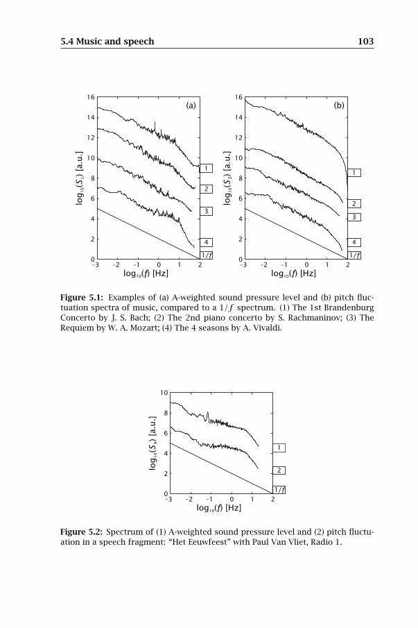
5.4 Music and speech 103
16
14
12
10
8
6
4
2
00 1 2–1–2–3
2
3
4
1
1/f
log
(1
0S
Z)
[a.u
.]
log ( ) [Hz]10 f
(b)16
14
12
10
8
6
4
2
00 1 2–1–2–3
2
3
4
1
1/f
log
(1
0S
L)
[a.u
.]
log ( ) [Hz]10 f
(a)
Figure 5.1: Examples of (a) A-weighted sound pressure level and (b) pitch fluc-tuation spectra of music, compared to a 1/f spectrum. (1) The 1st BrandenburgConcerto by J. S. Bach; (2) The 2nd piano concerto by S. Rachmaninov; (3) TheRequiem by W. A. Mozart; (4) The 4 seasons by A. Vivaldi.
10
8
6
4
2
00 1 2–1–2–3
2
1
1/f
log
()
[a.u
.]1
0X
S
log ( ) [Hz]10 f
Figure 5.2: Spectrum of (1) A-weighted sound pressure level and (2) pitch fluctu-ation in a speech fragment: “Het Eeuwfeest” with Paul Van Vliet, Radio 1.

104 1/f Noise in Rural and Urban Soundscapes
the 1/f dependence is recovered indicating a complex sequence of high
and low pitched voice passages. The 1/f dependence of pitch and level
fluctuation in music is explained by Voss and Clarke [329] as the result of
a critical balance between predictability and novelty. Later this result was
interpreted as music being an imitation of the self-organized criticality that
seems so common in nature.
5.5 Rural and urban soundscapes
Based on the theoretical considerations given in Section 5.2, it was ex-
pected that the 1/f dynamics of loudness and pitch could also be present
in outdoor soundscapes. Recordings were made at several different rural
locations at different times of day. The A-weighted sound pressure level,
loudness, and pitch power spectra for a selection of 6 typical rural sound-
scapes (in Flanders, Belgium) are presented in Figure 5.3. Although the
locations are specially selected as silent areas in Flanders (LAeq between 40
and 45 dB(A)), several man-made noise events could still be detected in
the recordings. Table 5.1 gives an overview of these events, grouped by
category external, rural, and natural sounds. The commercial airplanes
mentioned in the table pass at considerable height, resulting in a long, low
level background event.
The spectra given in Figure 5.3 in general show 1/f behaviour, but devi-
ate much more from this characteristic than music. Loudness spectra seem
to show a clearer trend than A-weighted level spectra. When amplifying the
recorded soundscape, the silent periods become filled with (low frequency)
sound that is probably caused by distant man-made noises such as traffic.
It is well known that, under most meteorological conditions, sound in the
frequency range of a few hundred Hertz propagates further than high fre-
quency sound. A-weighting does not adequately remove these unheard
components as Zwicker loudness [352] does, so they may peak up in the
Fourier spectrum of the amplitude fluctuation. Above 0.2 Hz, loudness de-
creases as 1/f but at longer time scales the frequency dependence can be
quite different. It is believed that this is due to the few loud events that
increase the contribution of slow variations. Pitch changes are also more
important below 0.2 Hz and are relatively independent of frequency above
this limit. A limited number of events (probably planes), changing the pitch
slowly, combined with relatively unpredictable pitch variation within the
event, can explain this.
Although wind induced noise was not dominantly present in any of the
soundscapes, it is still of interest to see that the wind velocity fluctuations

5.5 Rural and urban soundscapes 105
24
22
20
18
16
14
12
10
8
6
4
2
0210–1–2–3210–1–2–3210–1–2–3
1/f
R12
R11
R10
R9
R8
R7
log
(10
SX)
[a.u
.]
log ( ) [Hz]10 f
(c)(b)(a)
Figure 5.3: Spectrum of (a) A-weighted sound pressure level, (b) loudness and (c)pitch fluctuation, for 6 rural soundscapes.
Table 5.1: Noise events observed during rural soundscape recordings.
Category Event R7 R8 R9 R10 R11 R12
external distant traffic yes yes yes yes yes yestrain 1 1 1 1airplane sport 2 1 1 2airplane military 3 1airplane commercial 4 6 3 4 6 5loud recreation 5
rural local cars 1 2 3farm noises 2 5 10 2 2 2agriculture machine 1farm animals 5 15 25 15 15 5
natural birds yes yes yes yes yes yesinsectswind noiseswater

106 1/f Noise in Rural and Urban Soundscapes
8
6
4
2
0–1–2–3–4–5
log
()
[a.u
.]1
0V
S
log ( ) [Hz]10 f
Figure 5.4: Power spectrum of wind velocity fluctuation, observed during the pe-riod that soundscapes were recorded.
observed at a fixed location in the measurement area (measurements made
at 10 second intervals) have a power spectral density function following the
1/f law, at least down to about 10−3 Hz (Figure 5.4).
Urban soundscapes were recorded in the city of Ghent, Belgium. In
Table 5.2 the sites where soundscapes were recorded are described. The
power spectra of fluctuation in A-weighted sound pressure level, loudness,
and pitch are shown in Figure 5.5 for these 12 soundscapes. The general
1/f trend is again obvious. As for the rural soundscapes, the loudness
fluctuation spectrum gives a clearer picture than the A-weighted sound
pressure level fluctuation spectrum. For urban soundscapes, just as it was
the case for rural soundscapes, often a breakpoint seems to occur between
0.1 Hz and 1 Hz.
In an attempt to reduce data for further analyses, the frequency in-
terval is therefore split into two parts: I1 = [0.002 Hz, 0.2 Hz] and I2 =
[0.2 Hz, 5 Hz]; I3 = I1 ∪ I2 is the full frequency range. I2 corresponds to
a time interval between 200 ms and 5 s and can therefore be seen as char-
acteristic for the sound fluctuations emerging from the source itself (the
song of birds, voices, or the changes in the murmur of a passing plane). I1corresponds to the interval between 5 s and about 10 min. It is therefore
influenced mainly by sources such as cars, trains, planes, or talking people
passing the observer. In each interval, the slope, α, of a linear fit on the
log-log chart is calculated together with the squared fitting error, ǫ. This is
done both for the loudness and for the pitch fluctuations and thus results
in twelve possible indicators for the dynamics of each soundscape. The re-
sult is given in Table 5.3 and Table 5.4. For loudness, the α’s obtained for
frequency interval I2 are sufficiently close to −1 to call this behaviour 1/f

5.5 Rural and urban soundscapes 107
Table 5.2: Description of the urban settings where soundscapes were recorded.
Label Description
G1 Quiet green residential area in the center of town, medieval built uparea preventing intrusion of city sounds, occasional car, a few groupsof talking people and playing children around.
G2 Residential area at the edge of town, close to green open area, somemaintenance activity, a few people around, occasional bird, occa-sional airplane.
G3 Narrow street canyon, shops and offices, with car traffic (close tosaturation) and streetcar. Talking people passing by.
G4 Tourist attracting embankment in the car free center of the city.Many pavements with people talking, laughing, some bicycles andwalking people, distant music.
G5 Open square in the center of town with very restricted car traffic,but with public bus traffic and a streetcar passing every few min-utes, occasional bell. People sitting and talking at the many outdoorrestaurants and pubs, one of them singing loud during part of theobservation time.
G6 Open square with a few trees. Inner city traffic (close to saturation)and people passing by although often near the edges of the square.
G7 Traffic free shopping street, crossing street with traffic close by. Sev-eral delivery trucks pass by close in this small street canyon andsome unloading is going on. People passing by, sometimes talking,an occasional biker, church bells ring for a few minutes.
G8 Blocks of flats in open green setting just inside the ring road whichis relatively close by, occasional car passing by between the blocks,playing children, occasional passers by.
G9 Park area with private villas, railway station and two major roadsentering the city. A lot of park birds, pigeons, a few playing children,a few local cars.
G10 Inner city residential area, closely built up, a few trees, cars com-ing in, stopping, leaving. There is also some building activity, somechurch bells can be heard in the distance, occasionally small groupsof talking people on foot.
G11 One of the most important shopping streets with a dense stream oflively talking people passing by. No car traffic, but an occasionalstreetcar.
G12 Blocks of flats in open green setting near the major city sportingfacilities, including water features and bushy areas. Important localtraffic at short distance, several airplane, occasional loud recreation,in general an unexpectedly busy area.

108 1/f Noise in Rural and Urban Soundscapes
42
40
38
36
34
32
30
28
26
24
22
20
18
16
14
12
10
8
6
4
2
0210–1–2–3210–1–2–3210–1–2–3
1/f
G12
G11
G10
G9
G8
G7
G6
G5
G4
G3
G2
G1
log
(10
SX)
[a.u
.]
log ( ) [Hz]10 flog ( ) [Hz]10 flog ( ) [Hz]10 f
(c)(b)(a)
Figure 5.5: Spectrum of (a) A-weighted sound pressure level, (b) loudness and (c)pitch fluctuation, for 12 urban soundscapes.

5.5 Rural and urban soundscapes 109
Table 5.3: Slope α and quadratic error ǫ of a linear fit on the loudness spectraldensity in the three frequency-intervals.
Label LAeq I1 I2 I3α ǫ α ǫ α ǫ
R7 44.3 −1.64 0.56 −0.95 0.55 −1.16 0.56R8 42.6 −1.54 0.47 −0.94 0.57 −1.13 0.58R9 42.2 −1.57 0.51 −1.06 0.55 −1.26 0.55
R10 43.3 −1.96 0.54 −1.01 0.57 −1.26 0.58R11 40.9 −2.11 0.63 −0.91 0.55 −1.20 0.57R12 48.7 −2.16 0.55 −1.26 0.55 −1.31 0.56G1 51.0 −1.33 0.51 −0.88 0.55 −0.97 0.55G2 54.4 −1.17 0.47 −0.94 0.56 −1.06 0.56G3 65.5 −0.88 0.56 −0.91 0.55 −1.14 0.56G4 62.8 −0.54 0.49 −0.86 0.55 −0.94 0.55G5 65.1 −0.94 0.63 −1.18 0.58 −1.17 0.58G6 74.0 −1.67 0.65 −0.87 0.57 −1.12 0.58G7 57.7 −0.78 0.53 −1.06 0.56 −1.15 0.56G8 59.7 −0.56 0.40 −0.82 0.56 −1.04 0.57G9 51.3 −1.17 0.59 −0.91 0.55 −1.04 0.55G10 57.3 −1.73 0.53 −1.09 0.57 −1.14 0.57G11 65.3 −1.22 0.50 −0.92 0.56 −1.05 0.56G12 50.9 −1.11 0.48 −0.84 0.55 −1.08 0.56
by common convention; for pitch, soundscapes R11 and R12 seem to be-
have somewhat different. In the lower frequency interval I1, more variance
in the α’s is observed.
Clustering of the soundscapes based on sound levels leads to a group-
ing of quieter and louder soundscapes. Since the power spectral density of
loudness and pitch, and in particular its slope, gives additional information
on the dynamics of the soundscape, clustering based on the 12 indicators
derived above may uncover another dimension. Hierarchical clustering us-
ing the spss software [296] based on within group linkage is performed.
Figure 5.6 gives the results if Pearson’s correlation is used as a measure
of linkage. In this figure, linkage between groups of soundscapes further
to the right indicates a weaker coupling. Two large groups emerge. One
of them contains all rural soundscapes and a selection of urban settings.
In particular G6 and G10 remain members of this group for various other
choices of the parameters used for hierarchical clustering. At first sight,
these urban soundscapes have nothing in common with the rural setting.
G6 in particular has a very high LAeq. Clustering plots showed that the in-
terval I1 is the most important discriminator between the two large groups.
All rural soundscapes and the urban settings G6, G10, and to a lesser ex-

110 1/f Noise in Rural and Urban Soundscapes
Table 5.4: Slope α and quadratic error ǫ of a linear fit on the pitch spectral densityin the three frequency-intervals.
Label I1 I2 I3α ǫ α ǫ α ǫ
R7 −1.49 0.53 −0.93 0.55 −1.21 0.57R8 −1.71 0.66 −1.06 0.55 −1.23 0.56R9 −1.00 0.41 −0.86 0.56 −1.09 0.57
R10 −1.56 0.70 −0.89 0.55 −1.14 0.57R11 −1.35 0.41 −0.76 0.56 −1.04 0.57R12 −0.98 0.21 −0.74 0.57 −1.07 0.58G1 −1.20 0.62 −0.85 0.58 −0.83 0.58G2 −0.57 0.26 −0.81 0.55 −1.03 0.55G3 −0.64 0.32 −0.94 0.57 −1.14 0.57G4 −0.75 0.34 −0.81 0.55 −1.06 0.56G5 −0.19 0.25 −1.09 0.54 −1.16 0.54G6 −1.41 0.51 −1.04 0.56 −1.24 0.57G7 −0.89 0.41 −0.90 0.56 −1.08 0.56G8 −0.42 0.19 −0.99 0.56 −1.22 0.57G9 −0.81 0.40 −1.04 0.55 −1.21 0.55
G10 −1.50 0.56 −1.18 0.55 −1.29 0.56G11 −0.86 0.39 −1.02 0.55 −1.06 0.55G12 −0.54 0.37 −0.99 0.53 −1.13 0.53
tent G1 have in common that a few sound events peak considerably above
a more constant background noise. In the urban soundscape G6, this back-
ground is quite hurly-burly but when the recording is played back more
quietly, the similarities to suburban soundscapes become obvious.
There are clearly too many indicators extracted to describe the shape
of the power spectral density of loudness and pitch fluctuations for them
to be of any practical use.
pca analysis (including rotation) of the data shown in Tables 5.3 and 5.4
together with LAeq, resulted in four underlying variables explaining 78 % of
the variance in the data. The grouping of variables did not result in eas-
ily interpretable conclusions. The second component includes LAeq and
combines it with slopes in loudness and pitch spectra in interval I1. Hi-
erarchical clustering based on the same method as used for soundscape
clustering also allows clustering variables. The result is represented graph-
ically in Figure 5.7. It is clearly observed that the variables extracted for
interval I3 do not add much information to the variables extracted for I2since they are always grouped in an early stage (at the left hand side of the
figure). LAeq seems to be very close to slopes in power spectral density of
loudness and pitch for the interval I1. This is probably because both are
an indication of the presence of (loud) events in the soundscape.

5.5 Rural and urban soundscapes 111
G5
G8
G3
G7
G4
G12
G2
G11
G9
R12
R11
R9
R10
R8
G1
G10
G6
R7
2520151050
Figure 5.6: Dendrogram showing the result of hierarchical clustering of the sound-scapes, based on average within group linkage.
( , )N I1ǫ( , )Z I1ǫ( , )N I3ǫ( , )N I2ǫ
LAeq
( , )Z I1α( , )N I1α( , )N I3α( , )N I2α( , )Z I3α( , )Z I2α( , )Z I3ǫ( , )Z I2ǫ
2520151050
Figure 5.7: Dendrogram showing the result of hierarchical clustering of the indi-cators, based on average within group linkage.

112 1/f Noise in Rural and Urban Soundscapes
5.6 Discussion and conclusions
Theoretical considerations led to the conclusion that self-organization is so
common in many of the activities that together generate the rural and urban
soundscape, that a linear behaviour on a log-log scale of the power spec-
tral density of loudness and pitch fluctuations had to be found in sound
recordings made in these settings.
The most important finding of this chapter is that the expected 1/f
behaviour, previously found in music, also appears in many soundscapes.
However, this conclusion should be refined. It is quite common to find 1/f
in the frequency interval [0.2 Hz, 5 Hz]. That is, the region corresponding
to time scales of the order of a few seconds. It is dominated by fluctuations
in pitch and loudness of the source itself. On longer time scales, that is, in
the frequency interval [0.002 Hz, 0.2 Hz], the power spectrum differs signif-
icantly. In all rural soundscapes there are more slow variations in loudness
and pitch than expected in the case of soc. This is an indication of pre-
dictability and is caused by single cars and planes passing by and heard
from far away. Some of the urban soundscapes show this same charac-
teristic although they may be much louder on the average. In other urban
soundscapes 1/f or even a flatter spectrum is observed in this frequency
interval. Therefore, self-organization may indeed be more common here.
It can be attributed to traffic flows near saturation, mainly heard at a dis-
tance in the soundscapes that were studied, or to flocks of people passing
by in shopping or busy entertainment areas.
For cataloguing, indicators based on loudness and pitch power spec-
trum with log-log linearity corresponding to time intervals longer than
5 seconds are of interest, since they tend to be more complementary to
average loudness and LAeq. However, from a perception point of view,
higher frequencies, thus shorter time scales may be more indicative.
It is not the goal of the present chapter to interpret these observations
in terms of perception. Future work will have to draw this connection.
From findings with music, some indications can however be given. On the
shorter time scale (< 5 s), the 1/f observed in many of the soundscapes
indicate that their dynamics is quite interesting. For some of the rural
soundscapes the pitch power spectrum is too flat (e.g. R11 and R12). In
terms of the music results, this indicates that the pitch is too chaotic, not
predictable enough.
For longer time intervals, the loudness slope in most of the rural sound-
scapes is steeper than 1/f . Again extrapolating the findings from music,
this is an indication of too much predictability. This may be identified as
boring in terms of loudness. The loudness dynamic in most of the urban

5.6 Discussion and conclusions 113
soundscapes is less predictable as indicated by a 1/f or even flatter fre-
quency dependence. In the latter case loudness dynamic may even start to
sound too chaotic, too unpredictable to be music-like. The reason for this
dependence may be quite different as indicated by the two examples G4 and
G8. It could be very instructive to link this unpredictability, especially in
time intervals corresponding to I1, to the mitigating effect of predictability
on the harmful effect of noise on man [121] in future research.

Chapter6
The Temporal Structure of
Urban Soundscapes
D. Botteldooren, B. De Coensel and T. De Muer
Published in Journal of Sound and Vibration 292(1–2):105–123, 2006.
« « «
This chapter draws on the analogy between environmental sound-
scapes and music to propose an indicator for studying the temporal
structure of the urban soundscape. The influence of road traffic noise
on the new indicator is analyzed in detail. Results of this research were
presented at the Joint Congress of the French and German Acoustical
Society (CFA/DAGA ’04) [40].
6.1 Introduction
During the past few decades, studies on the effect of noise on man have
focused on physical and mental health, trying to relate it directly or in-
directly to noise exposure level. In many situations the unwanted health
effect, sleep disturbance, or annoyance can be related to one particular in-
truding sound. Soundscape research takes a more holistic approach. The
urban acoustic environment is regarded as an aggregate of many sounds
that can evoke specific emotions. The soundscape is seen as an integral
part of the urban living environment. This way, the soundscape is not
studied in isolation, but is interwoven within the whole context of visual
environment (landscape), feeling of safety, perceived air quality, etc. Mis-
match between different components of the living environment, including

116 The Temporal Structure of Urban Soundscapes
soundscape, may be at least partly responsible for a negative evaluation of
its quality.
Urban soundscapes emerge naturally as a result of the typical activi-
ties that take place in the public area. Over time, urban soundscapes have
evolved. Today, in many cases road traffic noise dominates the sound-
scape, often implying impoverishment and dulling of the living environ-
ment. Therefore, soundscape design should be included in future urban
planning and mobility planning. This requires the selection and use of a
number of quality indicators for the acoustic field.
To describe the outdoor acoustic field, some indicators have become
very commonly used. The A-weighted averaged sound level LAeq has tradi-
tionally been used as a primary indicator because it is easy to measure and
to calculate and it correlates reasonably well with perceived loudness and
specific annoyance. For non-specific, retrospective noise annoyance rating
of the immediate vicinity of one’s dwelling, night (and evening) seems to
play an important role. Hence Ldn (or Lden) is chosen as a suitable indicator
for long-term assessment.
An overview of recent developments in the area of urban soundscape
research and relevant indicators for the acoustic field can be found in [193].
Field investigation has identified a number of principal components in
the subjective description of urban soundscapes [171, 20, 325]. Gener-
ally speaking, loudness related cues come out as an important component,
but a factor related to the spectral structure [17] and one related to the
temporal structure also often emerge. Sound quality measures have been
suggested for soundscape analyses [118, 119] since they tend to capture
loudness, spectral content and short time fluctuations in a way that is more
closely related to subjective preference. Although often mentioned in rela-
tion to noise annoyance, studies on the influence of supra-second temporal
structure have been very rare. Bjork [26] has reported laboratory research
on the relation between temporal structure and (specific) annoyance, con-
spicuousness, and startle. They concluded that LAeq is an appropriate in-
dicator, at least for annoyance and for the sound stimuli used. However, in
relation to the present study it should be mentioned that all stimuli were
periodic and rather artificial in nature.
This chapter presents an indicator for the temporal structure of urban
soundscapes that is inspired by music research. Section 6.2 relates ur-
ban soundscapes to music and self-organized criticality. The latter is so
common in natural processes (and natural soundscapes) that music can
be thought of as an imitation of this particular temporal structure. Sec-
tion 6.3 introduces an indicator and applies it to categorize a set of sounds.
The new indicator is contrasted with classical indicators of environmental
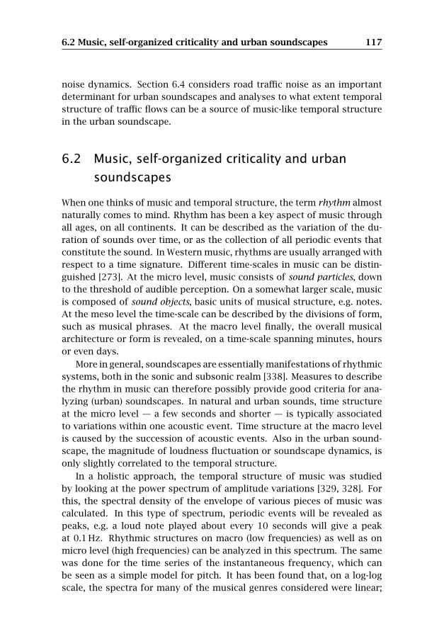
6.2 Music, self-organized criticality and urban soundscapes 117
noise dynamics. Section 6.4 considers road traffic noise as an important
determinant for urban soundscapes and analyses to what extent temporal
structure of traffic flows can be a source of music-like temporal structure
in the urban soundscape.
6.2 Music, self-organized criticality and urban
soundscapes
When one thinks of music and temporal structure, the term rhythm almost
naturally comes to mind. Rhythm has been a key aspect of music through
all ages, on all continents. It can be described as the variation of the du-
ration of sounds over time, or as the collection of all periodic events that
constitute the sound. In Western music, rhythms are usually arranged with
respect to a time signature. Different time-scales in music can be distin-
guished [273]. At the micro level, music consists of sound particles, down
to the threshold of audible perception. On a somewhat larger scale, music
is composed of sound objects, basic units of musical structure, e.g. notes.
At the meso level the time-scale can be described by the divisions of form,
such as musical phrases. At the macro level finally, the overall musical
architecture or form is revealed, on a time-scale spanning minutes, hours
or even days.
More in general, soundscapes are essentially manifestations of rhythmic
systems, both in the sonic and subsonic realm [338]. Measures to describe
the rhythm in music can therefore possibly provide good criteria for ana-
lyzing (urban) soundscapes. In natural and urban sounds, time structure
at the micro level — a few seconds and shorter — is typically associated
to variations within one acoustic event. Time structure at the macro level
is caused by the succession of acoustic events. Also in the urban sound-
scape, the magnitude of loudness fluctuation or soundscape dynamics, is
only slightly correlated to the temporal structure.
In a holistic approach, the temporal structure of music was studied
by looking at the power spectrum of amplitude variations [329, 328]. For
this, the spectral density of the envelope of various pieces of music was
calculated. In this type of spectrum, periodic events will be revealed as
peaks, e.g. a loud note played about every 10 seconds will give a peak
at 0.1 Hz. Rhythmic structures on macro (low frequencies) as well as on
micro level (high frequencies) can be analyzed in this spectrum. The same
was done for the time series of the instantaneous frequency, which can
be seen as a simple model for pitch. It has been found that, on a log-log
scale, the spectra for many of the musical genres considered were linear;
118 The Temporal Structure of Urban Soundscapes
moreover the slope always corresponded to 1/f at the macro level down
to the length of the piece [329, 328]. Figure 5.1 (previous chapter) shows a
few examples of amplitude (SL) and pitch (SZ) envelope spectra for different
musical genres. In view of application of this technique for outdoor sound,
the short-time A-weighted level time series of the acoustic signal can be
used as the amplitude envelope, as it will be demonstrated in the next
section.
In 1987 Bak et al. [8] introduced the notion of self-organized criticality
(soc) to explain 1/f noise. Although it is doubtful that their initial model
actually succeeded in predicting 1/f dynamics, self-organized criticality is
now generally believed to be a source of linear log-log behaviour of complex
systems [66, 76]. So in creating music, man seems to imitate the tempo-
ral fluctuation of self-organized critical systems, which are quite common
in the (natural) living environment. The observation that most listeners
found artificial 1/f type music more pleasing than artificial music showing
a flatter or a steeper spectral slope [329] was also found to be correlated to
characteristics of the chaotic dynamics observed in electroencephalograms
of subjects listening to this music [161].
Based on the above observations, it must be concluded that the spec-
trum of loudness and pitch variations of a sound fragment reveals impor-
tant characteristics of this sound fragment. Moreover, it seems reasonable
to assume that a straight spectrum in a log-log chart and in particular a
1/f characteristic contributes to the pleasing character of the sound. By
extension, this feature could be an interesting descriptor of urban sound-
scapes. In Chapter 5, it was shown that 1/f spectral characteristics could
indeed be found in the temporal pattern of amplitude and pitch in natural,
urban, and rural soundscapes. Figure 6.1 shows a few selected examples
where this characteristic is quite obvious. The observation of 1/f noise in
these sounds becomes far less surprising when recognizing the complex-
ity in the underlying systems as was shown in Chapter 5. As examples we
mention self-organized criticality that could arise under certain conditions
in the passage of talking people or the passage of cars on a highway. Com-
plex dynamics governing natural sound include the chorus of birds singing
or the sound of wind blowing in trees. It is needless to say that many ur-
ban soundscapes show a much less appealing temporal pattern than those
studied in this earlier work, mainly due to the dominating presence of road
traffic noise.
The relationship between appealing temporal structure of an urban
sound and impact indicators such as sleep disturbance or noise annoyance
is not trivial. Interesting, music-like temporal structure may become quite
disturbing or annoying when it intrudes unwantedly into ones living envi-

6.3 Descriptors for the temporal structure of a soundscape 119
20
18
16
10
8
6
4
2
0
14
12
0 1 2–1–2–3
N3
N4
R8
U9
1/f
R11
U11lo
g(
10
ZS
) [a
.u.]
log ( ) [Hz]10 f
(b)20
18
16
10
8
6
4
2
0
14
12
0 1 2–1–2–3
N3
N4
R8
R11
U9
U11
1/f
log
(1
0L
S)
[a.u
.]
log ( ) [Hz]10 f
(a)
Figure 6.1: Examples of (a) amplitude and (b) pitch spectra of natural (N3 & N4),rural (R8 & R11) and urban (U9 & U11) soundscapes, compared to a 1/f spectrum.
ronment. It is even reasonable to assume that a more predictable, boring,
and dull temporal structure is preferred in this case. Sound, presented as
artificial music to a listening panel, was found to be labeled too predictable,
boring, and dull if its amplitude and pitch spectrum had a slope steeper
than 1/f [329].
6.3 Descriptors for the temporal structure of a
soundscape
6.3.1 Descriptors based on the spectrum
A descriptor for the temporal structure of a soundscape is proposed, which
measures the similarity of its spectrum of loudness (and pitch) fluctuations
to those typical for music. Several choices need to be made. The time in-
terval of interest spans from a few hundred milliseconds to several min-
utes. It was already pointed out however that both for music and for urban
soundscapes a critical point could be identified, between time structure at
the micro and macro scale, around a few seconds. For music, this critical
point distinguished between the time structure determined by single notes
and that determined by the musical phrase and longer length scales. Com-

120 The Temporal Structure of Urban Soundscapes
1.0
0.8
0.6
0.4
0.2
0.01.00.80.60.40.20.0
deviation from straight line
mem
bers
hip
(b)1.0
0.8
0.6
0.4
0.2
0.00.0–0.5–1.0–1.5–2.0
slope
mem
bers
hip
(a)
Figure 6.2: Membership functions of the fuzzy sets describing (a) music-like slopeof the amplitude spectrum and (b) music-like deviation of the amplitude spectrumfrom a straight line. Both spectral intervals I1 (solid lines) and I2 (dashed lines)are considered.
paring the shorter length scale to urban noise seems less trivial because
of this prevalent presence of rhythm in music. The frequency interval of
interest is therefore split in I1 = [0.002 Hz, 0.2 Hz], I2 = [0.2 Hz, 5 Hz] and
I3 = I1∪I2. The descriptor must further include not only the average slope
of the spectrum but also a measure of its linearity (on a log-log scale). The
latter is described by the quadratic deviation from the best-fitted straight
line.
Careful investigation of the spectra in Figure 5.1 learns that the so-
called 1/f slope found for music is not all that strict. It may be more
appropriate to state that the amplitude and pitch spectrum of music has
an approximate 1/f or a 1/f -like behaviour. To quantify this vague state-
ment, a fuzzy set containing all slopes α that are found in music is ap-
propriate. The fuzzy set membership function is constructed on the basis
of the probability distribution [346] of slopes, derived from the spectra of
musical fragments, over the universe of slopes Uα. To extract this proba-
bility distribution, 15 samples of music of different genres (3 pop, 3 jazz,
9 classical) are analyzed. Smoothened membership functions of music-like
spectral slope, µA(α), are shown in Figure 6.2(a). Much in the same way, the
deviation of the spectrum from a straight line must be approached. Smaller
values of this deviation are more music-like, thus leading to the inclusive
fuzzy set membership functions, µE(ǫ), shown in Figure 6.2(b). Both sets
of membership functions are indexed by the spectral interval considered.
Set membership degrees (values of the membership function) close to one
mean perfect inclusion or a very music-like slope, α, or deviation, ǫ. Mem-
bership degrees close to zero mean that the spectrum is very unlike that
of music.

6.3 Descriptors for the temporal structure of a soundscape 121
Table 6.1: Selection based on ml1 of most music-like soundscapes out of 45.
Label Description ml1 ml1&2
R8 Rural environment, sounds of birds, sometimessounds from farm animals and a few farming ac-tivities, no local traffic, some distant traffic noiseoccasional commercial aircraft a high altitude.
1 0.35
U9 Traffic free shopping street in the center of Gent,talking people passing sometimes stopping for afew seconds, occasional biker, some distant mur-mur of car urban traffic, occasional (every 15 min-utes) church bell.
1 0.5
R11 Rural environment, very similar to R8. 1 0.5
N4 Remote rural environment at early morning, almostexclusively bird sounds, no man-made noise.
1 0.6
N3 Rocky coast, waves (approximately 0.5 m height)braking, little wind, occasional insect and one ortwo people silently passing by.
1 0.45
U1 Nature reserve at the edge of town, sounds of dif-ferent species of birds not particularly close, somewind in trees, occasionally talking people on bike.
0.95 0.05
U11 Urban park in residential area, distant traffic of dif-ferent sorts (cars, motorbikes, trains) with occa-sionally distinguishable events, wind in trees, a fewbirds, a local car about every minute.
0.95 0.7
Evaluation of degree of music-likeness of the temporal structure of a
soundscape is based on the measured slope in the spectrum of amplitude
fluctuations, α1 and α2, and on the deviation from a straight line of this
spectrum, ǫ1 and ǫ2. One of the following rules is used:
ml1 if α1 ∈ A1 and ǫ1 ∈ E1
then temporal structure of sound is music-like
ml1&2 if α1 ∈ A1 and ǫ1 ∈ E1 and α2 ∈ A2 and ǫ2 ∈ E2
then temporal structure of sound is music-like
The mathematical algorithm to calculate ml1 is described in more detail
in Appendix A. As an illustration of the use of these descriptors, Table 6.1
and Table 6.2 contain resp., a verbal description of the most music-like and
the least music-like soundscapes out of recordings at 45 randomly chosen
locations (typical duration of a recording is 15 minutes). Not surprisingly,
the most music-like samples contain a variety of sounds from only weakly
correlated sources. The least music-like ones are often dominated by a
single source. In some cases this source is present most of the time (e.g.

122 The Temporal Structure of Urban Soundscapes
Table 6.2: Selection based on ml1 of least music-like soundscapes out of 45.
Label Description ml1 ml1&2
U16 Urban street canyon in residential area, between400 and 600 vehicles per hour.
0.05 0
U17 Urban street canyon in residential area, between100 and 200 vehicles per hour.
0.05 0
U18 Urban street in residential area, between 500 and600 vehicles per hour, highway on flyover in thedistance.
0.05 0
R12 Rural area, a number of loud recreational events,one low flyover of a military aircraft, in betweensounds of birds and some distant road traffic.
0.05 0
U20 Urban road, two lane access road carrying between2000 and 2500 vehicles per hour.
0.05 0
R14 Rural area close to railway, natural sounds and windin trees are most important noise sources betweentrain passages.
0.05 0
U2 Urban road with shopping facilities, slow car trafficand tram passing by in groups (about 500 vehiclesper hour), few talking people.
0.05 0
U21 Urban road, two lane access road carrying between2000 and 2500 vehicles per hour.
0 0
U23 Busy highway in open area at a distance of about100 m.
0 0
U19 Urban street canyon in residential area, between200 and 300 vehicles per hour, some talking peo-ple passing.
0 0
busy traffic) but in others the source produces only a small number of loud
events per hour (e.g. train noise). Note also that the natural soundscapes
that show a very music-like temporal pattern are not very quiet ones. Very
quiet natural sites got rated worse because the constant background hum
was too predictable in comparison to the temporal structure of music.
6.3.2 Comparison to classical descriptors for dynamics
The generally accepted feeling that fluctuating noise is more annoying than
continuous noise, led to the construction of a number of indicators for
sound exposure that include a measure of level fluctuation. The Noise
Pollution Level [64] for example, LNP, is defined as LNP = LAeq + (LA10 −
LA90) or similarly LNP = LAeq + 2.56σ , where σ is the standard deviation of
the sound level.

6.3 Descriptors for the temporal structure of a soundscape 123
0
5
10
15
20
25
30
35
1.00.80.60.40.20.0
LL
A5–
[dB(A
)]A
95
ML
Figure 6.3: Music-like temporal structure ml1 ( ) and ml1&2 ( ) compared toLA5 − LA95 as a classical measure of dynamics, illustrated for 31 soundscapes.
For 31 soundscapes, the music-like temporal structure was obtained
using the rules ml1 and ml1&2. In Figure 6.3 this result is compared to
LA5 − LA95 as a classical indicator of dynamics. This figure shows that
there is some correlation between both descriptors (Pearson r 2 = 0.25 for
ml1 and r 2 = 0.07 for ml1&2). Some correlation is clearly expected as
it was already mentioned that quiet environments disturbed by the occa-
sional loud event have a low score on being music-like while at the same
time LA5 − LA95 will be high. The scattered points indicate that the new de-
scriptor that is proposed, probes a different dimension of the soundscape.
To further illustrate how the spectral shape gives additional information,
the sound level distribution and amplitude spectrum of two very different
sounds is shown in Figure 6.4. Both sounds have very similar distribu-
tions, although shifted in amplitude, but their spectrum is quite different.
Indeed the sound of the highway consists of a large number of short ran-
dom events. The level fluctuation of rustling of wind in trees is governed
by slow variations in wind velocity. Since these fluctuations in wind veloc-
ity are the result of a complex phenomenon, the spectrum of amplitude
fluctuations corresponds better to a straight line for this second sound.
6.3.3 Relation to urban soundscape perception
It is our opinion that the relationship between the proposed descriptor for
urban soundscape temporal structure and music, and the proven effect of
music and music-like noise on mental state and possibly on health, are

124 The Temporal Structure of Urban Soundscapes
80
65
50
35
75
70
60
55
45
40
30
25
200.15 0.200.100.050.00
N5
U23
LA
,fast[d
B(A
)]
sample probability
(b)12
11
10
4
3
2
1
0
5
6
7
8
9
0 1–1–2–3
N5
U23
1/f
log
(1
0L
S)
[a.u
.]
log ( ) [Hz]10 f
(a)
Figure 6.4: Examples of (a) amplitude spectrum compared to a 1/f spectrum and(b) sound level distribution for two very different sounds: (U23) the sound of ahighway at short distance and (N5) the rustling of wind in trees.
sufficient to justify its introduction. Nevertheless it would be interesting
to find out how the temporal structure of the soundscape influences the
evaluation by an accidental user of its urban context. A small-scale survey
involving one hundred subjects and ten urban sites was set up as a pilot
project. Since temporal structure involves time scales of several minutes
to a quarter of an hour, the questions had to have a retrospective character.
Having people stand and listen to the urban sound for a quarter of an hour
would just be too boring. Since the focus of this study is on soundscape
characterization rather than on perception of sound, it was decided to sep-
arate the assessment based on the physical indicators from the interviews.
The only two variables that were controlled were the season and the fact
that it did not rain during any of the days of the experiment. The sam-
ple of passers-by was drawn at random, not controlling for age or gender
between the sites because there is an obvious natural bias.
Asking lay people about the temporal structure of a soundscape and its
resemblance to music is impossible. The extent to which they can hear the
music in urban sounds may depend strongly on their socio-cultural back-
ground and previous experience with more experimental types of music.
Moreover, it could be expected that asking about music would trigger dif-
ferent foci, e.g. tonality, beat… than the one envisaged in this work. To

6.3 Descriptors for the temporal structure of a soundscape 125
music- like
boring/dull
chaotic
Figure 6.5: Triangular answer scale used in the survey.
clarify the context, inspiration was found in the work of Voss and Clarke
on music [329]. With respect to the slope in the spectrum of amplitude
and pitch variations, it was found that a slope steeper than 1/f resulted
in sound that was labeled too boring and dull to be music, while a flatter
slope resulted in a sound that was too chaotic and unpredictable to be mu-
sic. Therefore it was decided to contrast music-like to boring/dull at one
hand and to chaotic at the other hand. Because of the other connotations of
music, it was decided not to place the label “music” exactly between chaotic
and boring/dull as the work on temporal structure of music theoretically
predicts. Instead the labels were put on a triangular scale (Figure 6.5) and
people were asked to put a mark in between the three points. Since the
survey is conducted face-to-face, additional clarification of this rather dif-
ficult scale allows the average person to use it to express an opinion. The
distance to each corner is measured for further analyses.
The relation between music-like temporal structure extracted from the
spectral slope (ml1) and distance (average and 95 % confidence intervals)
to the three points in the subjective scale, is given in Figure 6.6(a–c) for
the ten sites that were considered. The confidence intervals are relatively
large, indicating the strong influence of other factors on the evaluation.
Some personal factors can be expected to have an influence, but due to
the limited size of the sample this could not be investigated. The clearest
trend is seen for the distance from “chaotic”. Soundscapes at sites where
the objective parameter ml1 is high are subjectively rated further from
chaotic. The subjective rating for music-like character shows the expected
opposite trend: high ml1 corresponds to smaller distance to the subjective
rating music-like. This trend is less pronounced. The subjective distance
to boring/dull shows a trend that is opposite to what could be expected.

126 The Temporal Structure of Urban Soundscapes
1.0
0.8
0.6
0.4
0.2
0.03020100
distance from “not music- like”
ML1
(d)1.0
0.8
0.6
0.4
0.2
0.05040302010
distance from “boring”
ML1
(c)
1.0
0.8
0.6
0.4
0.2
0.0403020100
distance from “chaotic”
ML1
(b)1.0
0.8
0.6
0.4
0.2
0.040302010
distance from “music- like”
ML1
(a)
Figure 6.6: Subjective evaluation of soundscapes in a triangle with the cornersrepresenting music-like, chaotic and boring/dull, compared to the music-like tem-poral structure ml1. Averages and 95 % confidence intervals are shown.
Again inspired by the results obtained with music, a new variable was con-
structed that measures the shortest of the distances to boring/dull and
chaotic. This variable was labeled “not like music” because both character-
istics indicate that the temporal structure of the sound does not match a
temporal structure that allows for this sound to be labeled “music”. The
correlation of this variable with ml1 is not much higher than the correlation
of the variable “distance to chaotic”, as can be seen in Figure 6.6(d).
There are several methodological issues that may influence these re-
sults. Both the subjective perception and ml1 may be correlated to par-
ticular features of the sonic environment (e.g. the amount of road traffic)
without being correlated to each other directly. Also, personal characteris-
tics of typical passers-by may be different at different locations resulting in
different average subjective evaluation not correlated directly to the noise
itself. However, this small-scale study seems to confirm some of the obser-
vations made by trained acousticians. The unexpected low value ml1 = 0.23
for the fourth soundscape from below in Figure 6.6 was also surprising for
a trained observer. The broad confidence interval for the fifth soundscape
from below in Figure 6.6 seems to reflect the strongly changing character
of the soundscape at this open urban square that was also noticed by the
trained observer.
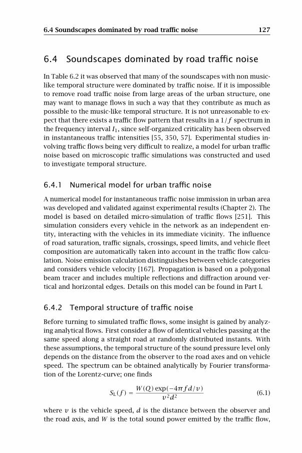
6.4 Soundscapes dominated by road traffic noise 127
6.4 Soundscapes dominated by road traffic noise
In Table 6.2 it was observed that many of the soundscapes with non music-
like temporal structure were dominated by traffic noise. If it is impossible
to remove road traffic noise from large areas of the urban structure, one
may want to manage flows in such a way that they contribute as much as
possible to the music-like temporal structure. It is not unreasonable to ex-
pect that there exists a traffic flow pattern that results in a 1/f spectrum in
the frequency interval I1, since self-organized criticality has been observed
in instantaneous traffic intensities [55, 350, 57]. Experimental studies in-
volving traffic flows being very difficult to realize, a model for urban traffic
noise based on microscopic traffic simulations was constructed and used
to investigate temporal structure.
6.4.1 Numerical model for urban traffic noise
A numerical model for instantaneous traffic noise immission in urban area
was developed and validated against experimental results (Chapter 2). The
model is based on detailed micro-simulation of traffic flows [251]. This
simulation considers every vehicle in the network as an independent en-
tity, interacting with the vehicles in its immediate vicinity. The influence
of road saturation, traffic signals, crossings, speed limits, and vehicle fleet
composition are automatically taken into account in the traffic flow calcu-
lation. Noise emission calculation distinguishes between vehicle categories
and considers vehicle velocity [167]. Propagation is based on a polygonal
beam tracer and includes multiple reflections and diffraction around ver-
tical and horizontal edges. Details on this model can be found in Part I.
6.4.2 Temporal structure of traffic noise
Before turning to simulated traffic flows, some insight is gained by analyz-
ing analytical flows. First consider a flow of identical vehicles passing at the
same speed along a straight road at randomly distributed instants. With
these assumptions, the temporal structure of the sound pressure level only
depends on the distance from the observer to the road axes and on vehicle
speed. The spectrum can be obtained analytically by Fourier transforma-
tion of the Lorentz-curve; one finds
SL(f ) =W(Q) exp(−4πfd/v)
v2d2(6.1)
where v is the vehicle speed, d is the distance between the observer and
the road axis, and W is the total sound power emitted by the traffic flow,

128 The Temporal Structure of Urban Soundscapes
which depends, among other things, on the traffic intensityQ. Figure 6.7(a)
shows this spectrum for a few realistic combinations of distance, vehicle
speed and traffic intensity, which are given in Table 6.3. In the inter-event
time interval I1, the spectrum is rather flat indicating chaotic and unpre-
dictable temporal structure. At higher frequencies the decay is steep, an
indication of predictability on this shorter time scale. Random vehicle pass
by instants is not a very realistic model unless vehicle intensity is so low
that there is no interaction between the vehicles. Another extreme traffic
model assumes that the distance between vehicles is constant. This makes
the temporal structure periodic with a periodicity that reduces as traffic
intensity increases. The spectrum (Figure 6.7(b)) now peaks at a nonzero
frequency corresponding to this periodicity. As d/v increases this peak
becomes sharper. Because of the log-log plot, the peak is also more pro-
nounced as its frequency increases. From the soundscape perspective, this
implies that also in this second extreme traffic model, the temporal struc-
ture is far from music-like.
Let us now turn to more realistic traffic flows. Using the model described
in the previous section, part of the city of Ghent is modeled in detail (Fig-
ure 2.3). For each simulation, traffic is allowed to settle for 15 minutes
before the 15-minute acoustic simulation starts. Sound levels, averaged
over 0.5 seconds, are calculated for a number of locations in this test area
at a distance of 1 m from the façade. As a first example, the spectra of the
amplitude fluctuations and the sound level distributions at 10 locations
(one every 5 meter, parallel to the road axis) near measurement point 5 in
the map are shown in Figure 6.8. In the frequency interval [0.01 Hz, 1 Hz],
the spectrum resembles more that of a complex system than the analyt-
ical approximations of Figure 6.7, but the slope is not steep enough for
this sound to show clear music-like dynamics. The peak around 0.01 Hz is
caused by the periodicity of three sets of traffic lights in the vicinity of the
observation area. If traffic demand is increased to 160 %, traffic is almost
continuous during the green phase of the traffic lights. The spectral peak
at 0.01 Hz gets more pronounced as well as a few side peaks, leading to a
less music-like temporal structure (Figure 6.9).
To get a more complete picture of the effect of traffic intensity on the
temporal structure of the soundscape, the traffic demand on the main ac-
cess road that passes measurement point 5 is gradually increased from
zero to 220 % of today’s rush hour traffic in steps of 5 %. The indicator ml1
is calculated and averaged over 4 locations (one every 10 m) near point 5.
Figure 6.10(a) shows the increase of traffic intensity until the road totally
saturates (including a complete jam at 190 %) and the evolution of ml1.
Traffic noise shows a more music-like temporal structure as traffic satu-

6.4 Soundscapes dominated by road traffic noise 129
9.5
10.0
10.5
11.0
11.5
12.0
12.5
13.0
0–1–2–3
B2
B3
B4
B1
B5
log
(1
0L
S)
[a.u
.]
log ( ) [Hz]10 f
(b)
13
12
10
7
6
5
4
8
9
11
0–1–2–3
A2
A3
A4
A1
A5
log
(1
0L
S)
[a.u
.]
log ( ) [Hz]10 f
(a)
Figure 6.7: Spectrum of amplitude fluctuations of the noise from an analytic trafficflow: (a) random vehicle instants, (b) equidistant vehicles. Parameter values canbe found in Table 6.3.
Table 6.3: Parameter value combinations for the spectra shown in Figure 6.7.
Label d [m] v [km·h−1] Q [vehicles·h−1]
A1 20 90 200A2 20 50 200A3 20 30 200A4 50 50 200A5 100 50 200
B1 20 90 200B2 20 50 200B3 20 30 200B4 20 50 500B5 20 50 2000

130 The Temporal Structure of Urban Soundscapes
50
55
60
65
70
75
80
85
90
95
100
0.150.100.050.00
LA
,fast[d
B(A
)]
sample probability
(b)5.0
4.5
4.0
3.5
3.0
2.5
2.0
1.5
1.0
0.5
0.00–1–2–3
log
(1
0L
S)
[a.u
.]
log ( ) [Hz]10 f
(a)
Figure 6.8: (a) Amplitude spectrum and (b) sound level distribution around point 5in the map, with traffic at normal load during rush hour.
50
55
60
65
70
75
80
85
90
95
100
0.150.100.050.00
LA
,fast[d
B(A
)]
sample probability
(b)5.0
4.5
4.0
3.5
3.0
2.5
2.0
1.5
1.0
0.5
0.00–1–2–3
log
(1
0L
S)
[a.u
.]
log ( ) [Hz]10 f
(a)
Figure 6.9: (a) Amplitude spectrum and (b) sound level distribution around point 5in the map, with traffic at 160 % of normal load during rush hour.

6.4 Soundscapes dominated by road traffic noise 131
0
50
100
150
200
250
300
350
400
450
0.0
0.1
0.2
0.3
0.4
0.5
0.6
0.7
0.8
0.9
1.0
6005004003002001000
traffic
inte
nsity
[vehic
les/15m
in]
demand [% of rush hour]
ML1
(b)
0
50
100
150
200
250
300
350
0.0
0.1
0.2
0.3
0.4
0.5
0.6
0.7
0.8
0.9
1.0
250200150100500
traffic
inte
nsity
[vehic
les/15m
in]
demand [% of rush hour]
ML1
(a)
Figure 6.10: Average music-like temporal structure ml1 of the traffic noise ( ) andtraffic intensity on one lane ( ): (a) near location 5 as a function of traffic demand(in percentage of rush hour traffic) on the main access road; (b) near location 3 asa function of traffic demand on this local road.

132 The Temporal Structure of Urban Soundscapes
60
62
64
66
68
70
72
10
12
14
16
18
20
22
24
26
6005004003002001000
LA
eq[d
B(A
)]
demand [% of rush hour]
LL
A5–
[dB(A
)]A
95
(b)
69
70
71
72
73
74
75
76
10
11
12
13
14
15
16
17
18
19
20
250200150100500
LA
eq[d
B(A
)]
demand [% of rush hour]
LL
A5–
[dB(A
)]A
95
(a)
Figure 6.11: LA5 − LA95 ( ) and LAeq ( ): (a) near location 5 as a function of trafficdemand (in percentage of rush hour traffic) on the main access road; (b) nearlocation 3 as a function of traffic demand on this local road.

6.5 Conclusions 133
rates, but probability seems to play an important role as indicated by the
large spread in the points. Figure 6.11(a) shows the steady decrease of
LA5 − LA95 with traffic demand. This decrease in dynamics continues after
the road saturates and traffic intensity no longer increases.
As a second example, measurement point 3 is considered. Today, this
is a quieter road through a less built-up area. Traffic dynamics are hardly
influenced by traffic lights. Random generation of traffic at local nodes on
the other hand plays a much more important role. Figure 6.10(b) shows
the mild saturation of traffic and the evolution of ml1. Traffic noise turns
out to be much too random to be labeled music-like in this case. The small
peak in ml1 at a traffic demand that is 200 % of today’s value may corre-
spond to an onset of soc. It corresponds to a slight increase in number
of cars, corresponding to the general notion that the throughput is opti-
mal at socconditions. Figure 6.11(b) shows how the LAeq saturates more
quickly than the traffic intensity as a function of traffic demand, due to
the reduced vehicle speed. Also, LA5 − LA95 steadily decreases with traffic
demand, indicating the filling up of quiet intervals.
6.5 Conclusions
The temporal structure of an urban soundscape can accurately be described
by looking not only at the dynamics in terms of differences in statistical
noise levels, but also at the spectrum of amplitude (and pitch) fluctua-
tions. Since it was noticed that particular spectral features that relate to
self-organized criticality are present in most types of music (so called 1/f
noise), it is enlightening to look in particular for this feature in the tempo-
ral structure of urban soundscapes. By combining the requirement that the
spectrum must show a straight line on a log-log scale and that this straight
line must have a 1/f slope for the temporal structure to be music-like,
a fuzzy indicator for music-likeness (ml) was constructed. Environmen-
tal sound recordings were tested for this temporal structure and indeed it
was found in several natural and urban environments. At the same time
soundscapes with far from music-like temporal structure are also quite
common. For this latter group, two situations occur: either the temporal
structure is too predictable or it is too chaotic. In general it can also be
observed that music-like temporal structure is much more rare in sound-
scapes dominated by a single source.
A small-scale survey indicates that the ml characteristic does not corre-
late well with the feeling that the environmental noise sounds like music,
mainly because few subjects could imagine urban noise to be music. On
134 The Temporal Structure of Urban Soundscapes
the contrary, there seems to be a clearer relation to the soundscape being
neither chaotic nor boring.
Traffic noise is an important contributor to many urban soundscapes.
Using microsimulation of traffic flow, it has been shown that music-like
dynamics can emerge in traffic noise on the supra-event time-scale. Self-
organized criticality that emerges in the underlying traffic system is re-
sponsible for this behaviour. Unfortunately this is not a very common
situation in urban traffic noise. For free flow, traffic seems often to be too
random or too structured. Randomness is caused by local generation of
traffic. Traffic management in general, and traffic lights in particular, tend
to regulate flow in a more deterministic manner.
The indicator presented in this chapter sheds new light on how urban
soundscape quality might be assessed in an objective way. By using the
analogy with music, the indicator follows more closely the original ideas be-
hind urban soundscape research. Based on this, we argue that the proposed
indicator is a good candidate for describing and categorizing soundscape
temporal structure, and can be used in addition to loudness and spectral-
quality indicators (sharpness, roughness). There is an obvious need for
further analysis of the relation between this objective indicator and more
subjective evaluations of the quality of urban sound by an active partici-
pant. Dedicated research involving psychoacoustic lab research as well as
field investigation should be started in this field.

Chapter7
Artificial Sound through
Self-organization
7.1 Introduction
7.1.1 Evaluation of the temporal aspect
Evaluation of the impact of the temporal aspect on soundscape perception
is essential for a meaningful inclusion of this aspect in soundscape assess-
ment. To reach this goal, several paths may be followed. An often used
methodology in soundscape perception research consists of linking lin-
guistic terms (e.g. “pleasant”, “exciting”, “dull”, “stressful”…) to objective,
physical characteristics of the soundscape (loudness, sharpness, music-
likeness…). This may be accomplished by the use of listening tests, in
which sounds with controlled physical characteristics are presented. This
methodology implies that one knows the linguistic terms fitting well to a
given soundscape, which can be derived from on-site questionnaires.
A more direct approach would be to determine the most suitable sound-
scape to a given environment, and to extract the associated physical char-
acteristics. This could be accomplished by the use of listening tests with
visual/verbal input concerning the type of environment. This methodology
makes dealing with linguistic terms superfluous.
7.1.2 Information content of sound
However, physical characteristics do not grasp the meaning of sounds. To
the listener, a sound not only has a form, but also a content — each sound is
perceived as a carrier of information. Consequently, the meaning of sound

136 Artificial Sound through Self-organization
has a large influence on human perception. For example, sound quality in
general [160, 348], and loudness in particular [140, 91] are known to be
partly dependent on the meaning of the sound. As a consequence, noise
annoyance is also partly determined by meaning [92]. A well known exam-
ple is the railway bonus [221]: at the same LAeq, railway noise is preferred
to road traffic noise. Spectral differences and differences in the time struc-
ture between both types of noise can only account partly for the difference
in preference.
Even cultural background plays a role in the emotion a perceived sound-
scape may evoke. For example, an intercultural study with Japanese and
German test persons [185] showed that the sound of a bell is perceived in a
different way by both groups. The German subjects generally associated a
bell with the sound of a church, leading to feelings of pleasance and safety.
On the other hand, a bell reminded the Japanese subjects to a fire engine
or a railway crossing, leading to feelings of unpleasance and danger.
Based on the above considerations it is obvious that, in order to be able
to assess the fundamental characteristics of environmental noise, one has
to consider the information content associated with the sounds used care-
fully. To circumvent this difficulty, listening test sounds are sometimes
made unrecognizable. The classical methodology is to extract the tempo-
ral envelope by applying a low-pass filter and rectifying the output. This
temporal envelope is then used to modulate a pink noise source, leading to
an “unrecognizable” sound which has the same temporal envelope as the
original sound. However, the spectral characteristics of the original sound
are lost. To resolve this negative side effect, Fastl [97, 98] introduced a
method based on spectral analysis of the original sound. In essence, a spec-
tral broadening is applied to the fourier transform of the original signal.
An unrecognizable sound with the same amplitude and temporal structure,
and about the same spectrum as the original is then calculated using the
inverse fourier transform.
7.1.3 Artificial environmental soundscapes
The main disadvantage of the above method of making sounds unrecog-
nizable is that, to be able to conduct a listening test, a database of sounds
with desired characteristics has to be available. In this chapter, a more in-
novative methodology is outlined, in which it is proposed to use artificial
soundscapes, instead of departing from existing recordings. Using sounds
made unrecognizable or artificial sounds does not exclude the possibility
that a meaning is associated to the sound by the listener. For example,

7.1 Introduction 137
high frequency tonal sounds may remind the listener of birds. Therefore,
we rather speak of sound with reduced information content, instead of
meaningless sound.
Since we are mainly interested in the temporal aspect in this work, the
model for producing artificial soundscapes has to be flexible on this topic.
As it was explained in Chapter 5 that complex systems often show interest-
ing temporal characteristics, including 1/f noise, it would be favourable to
employ some sort of system which naturally shows a complex dynamic be-
haviour to produce artificial sound. As it turns out, dynamic systems have
been used extensively to create artificial music (see the reviews in [51, 214]
for some recent examples). In particular, swarm intelligence — an ai tech-
nique modeling the collective behaviour of a decentralized system of agents
— was already used to create expressive, freely “improvized” music by
Blackwell and Bentley [28, 27]. A particle system is simulated in the 3-
dimensional space. Several forces, both attractive and repulsive, govern
the movement of each particle, resulting in a complex aggregate behaviour.
At each timestep, each particle generates a midi event which is sent to a
midi synthesizer; the 3 particle coordinates are mapped to a value for the
loudness, pitch and duration of the event. The particles “swarm” around
an attractor, which may be adjusted interactively by a musician, creating
a “duet”. An interesting analogy can be drawn with the work of Voss and
Clarke [329], in which it was found that artificial music produced with a
1/f noise generator (which could be, for example, a complex system) is
perceived to be the most appealing.
The original model of Blackwell et al. was developed to create (tonal)
music, and is not able to reproduce broadband noise, which is common in
environmental soundscapes. In this chapter, we will therefore extend this
model to produce artificial environmental noise. The temporal structure
of this noise may be controlled indirectly, so it can be used as a basis
for listening experiments in which the test person has to select the best
fitting soundscape for a given environment. A drawback of this technique
is that the spectral and temporal structure of the artificial soundscape is
controlled by several parameters in a nonlinear fashion. As a consequence,
it would be hard for a test person to adjust these parameters to achieve a
suitable soundscape. This will be solved by applying a genetic algorithm
(ga) — another ai technique — to automatically optimize these parameters.
This will make the task of the test person much more simple, as only simple
decisions will have to be made.
In the following sections, each part of this model will be explained more
in detail.

138 Artificial Sound through Self-organization
7.2 Self-organizing particle swarms
7.2.1 Swarm intelligence
Since time immemorial, people have been fascinated by the variety of ani-
mal behaviour in nature. The aggregate motion of a flock of birds, a school
of fish or a group of ants has puzzled many. Recently, biologists and com-
puter scientists have studied and modeled these biological swarms, to un-
derstand how such animals interact, achieve goals and evolve (for example,
see [269, 308]). A swarm is typically made up of a population of animals,
interacting locally with one another and with their environment. Although
there is no centralized control structure dictating how individual animals
should behave, often a collective intelligent behaviour emerges, which is
called swarm intelligence [31] — this term was first introduced by Beni &
Wang [11] in the context of cellular robotic systems. Swarm intelligence is
an example of self-organization (see Section 4.3.1) in biological systems.
Engineers are interested in this kind of swarm behaviour, since the re-
sulting swarm intelligence can be used as a heuristic method to solve op-
timization problems. Usually, the swarm is implemented as a multi-agent
system: the data is decentralized and the execution is asynchronous (each
agent has its own thread). Several optimization techniques have been pro-
posed based on this paradigm, the most important being ant colony opti-
mization (aco), stochastic diffusion search (sds) and particle swarm opti-
mization (pso):
Ant colony optimization: In aco [60, 84, 306], artificial ants travel the so-
lution space. The ants initially wander randomly, but when a good
solution is found, they return to their colony and mark their path by
depositing artificial pheromone, mimicking real ants. If other ants
find such a path, they are likely to follow and reinforce the trail. aco
particularly has been applied succesfully to find (near-)optimal solu-
tions to the traveling salesman problem [132].
Stochastic diffusion search: sds [24, 77] is best suited for combinatorial
optimization problems in which the objective function can be decom-
posed into multiple independent partial functions. Information is
diffused between different agents across the population via one-to-
one communication, in contrast to the pheromone method used in
aco. sds has been applied succesfully to diverse problems such as
text search [24], object recognition [25] and site selection for wireless
networks [150].

7.2 Self-organizing particle swarms 139
Particle swarm optimization: pso [174] is a continuous optimization algo-
rithm dealing with problems in which a solution can be represented
as a point in a D-dimensional space. Inspired by the movement of a
flock of birds, a dynamic swarm of particles is simulated, in which the
position of each particle represents a possible solution. The move-
ment of a particle is governed by an attraction to the best position
it encountered so far, an attraction to the swarm’s best position, and
a random force introducing some craziness in its movement. pso is
especially resilient to the problem of getting trapped in local minima,
thanks to the large number of agents usually employed. The perfor-
mance of pso may further be improved by introducing dissipation of
energy [341], or by applying techniques borrowed from biological evo-
lution, such as mass extinction [342] or breeding [199]. pso has been
applied to various optimization problems, such as neural network
training, power system control or the traveling salesman problem; an
overview can be found in [59].
Optimization problem solving is not the sole field of application of
swarm intelligence based techniques; they have been applied succesfully
in diverse fields of science, technology and art, such as controlling a large
number of robots, or creating realistic animal swarm behaviour or mas-
sive battle scenes in movies. As already mentioned in the introduction of
this chapter, in [28] a specially tailored particle swarm technique is applied
to create artificial music. Only a small number of particles is used (usu-
ally 5, which is enough to make complex chords possible), in contrast to
pso techniques applied to optimization problems.
As already mentioned in Section 4.3.1, self-organization requires posi-
tive as well as negative feedback, which for pso is translated into particle
attraction and repulsion [31]. Therefore, a repulsive inter-particle force is
introduced in [28], to let the particles not swarm too close to each other —
this has as a consequence that the melody will not be too repetitive. soc
was not the main concern in [28], since the input of the human musician
involved in the performance already resulted in interesting music. In the
next paragraphs, we will discuss a generalization of this technique to D
dimensions, and we will show how the model can be extended with soc.
7.2.2 Particle swarm dynamics
Consider a swarm of N particles, traveling in a hyperspace of dimension
D. Each particle i = 1 . . . N is described by its massmi, its position -→x i and
its velocity -→v i. Initially, all particles are placed at random locations and
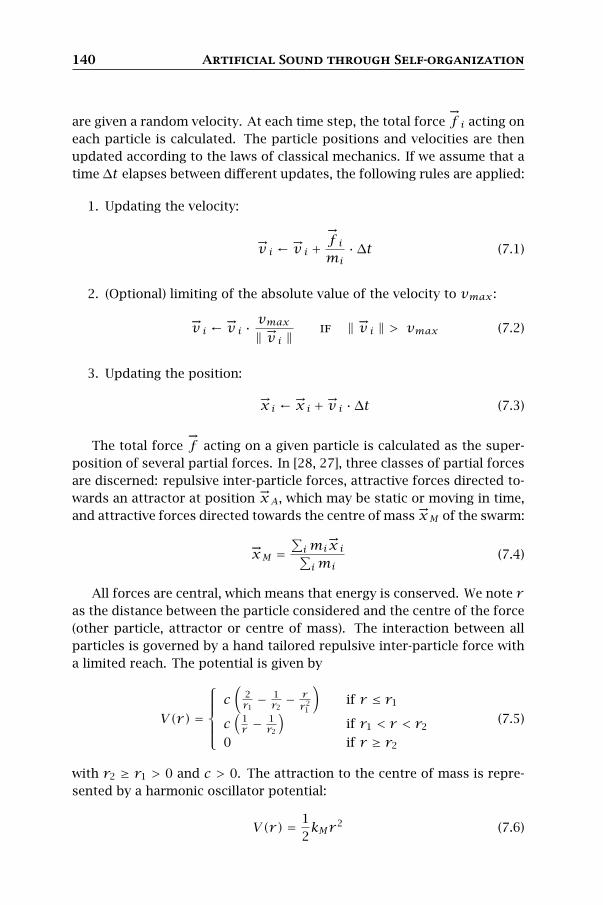
140 Artificial Sound through Self-organization
are given a random velocity. At each time step, the total force-→f i acting on
each particle is calculated. The particle positions and velocities are then
updated according to the laws of classical mechanics. If we assume that a
time ∆t elapses between different updates, the following rules are applied:
1. Updating the velocity:
-→v i ←
-→v i +
-→f i
mi·∆t (7.1)
2. (Optional) limiting of the absolute value of the velocity to vmax :
-→v i ←
-→v i ·
vmax
‖-→v i ‖
if ‖-→v i ‖ > vmax (7.2)
3. Updating the position:
-→x i ←
-→x i +
-→v i ·∆t (7.3)
The total force-→f acting on a given particle is calculated as the super-
position of several partial forces. In [28, 27], three classes of partial forces
are discerned: repulsive inter-particle forces, attractive forces directed to-
wards an attractor at position -→xA, which may be static or moving in time,
and attractive forces directed towards the centre of mass -→xM of the swarm:
-→xM =
∑imi
-→x i∑
imi(7.4)
All forces are central, which means that energy is conserved. We note r
as the distance between the particle considered and the centre of the force
(other particle, attractor or centre of mass). The interaction between all
particles is governed by a hand tailored repulsive inter-particle force with
a limited reach. The potential is given by
V(r) =
c
(2r1− 1r2− r
r21
)if r ≤ r1
c(
1r −
1r2
)if r1 < r < r2
0 if r ≥ r2
(7.5)
with r2 ≥ r1 > 0 and c > 0. The attraction to the centre of mass is repre-
sented by a harmonic oscillator potential:
V(r) =1
2kMr
2 (7.6)

7.2 Self-organizing particle swarms 141
Vr()
r
(d)
Vr()
r
(c)
Vr()
r
(b)
Vr()
r
(a)
Figure 7.1: Qualitative examples of potentials: (a) Inter-particle potential, (b) har-monic potential; (c) gaussian potential and (d) spherical well potential.
with spring constant kM . The attraction to an attractor is also represented
by a harmonic oscillator potential, with spring constant kA.
To make it possible that particles temporarily escape from the swarm or
from an attractor, an alternative potential was implemented in our model,
which has a gaussian shape:
V(r) = −ae−(r/b)2
(7.7)
The depth of the potential well is dependent on the parameter a, the width
on the parameter b.
In [28], the simulation space is bounded to a hypercube by putting crisp
limits on the particle coordinates. This may result in a non-smooth trajec-
tory for particles swarming near the border of the simulation space. In our
model we have therefore implemented a spherical well potential, which is
used to keep the swarm within a hypersphere with a soft border:
V(r) =
{0 if r ≤ bS12aS(r − bS)
2 if r > bS(7.8)
The steepness of the walls is dependent on the parameter aS , the radius
of the well on the parameter bS . Figure 7.1 shows an example of these
potentials.
142 Artificial Sound through Self-organization
7.2.3 Extending the technique with soc
The model described up to here follows the laws of mechanics, and shows
more resemblance to a complex planetary system than to our intuitive idea
of a swarm. As a possible way to add more diversity to the particle swarm
algorithm, a soc extension was already proposed in [201].
With each particle, an extra variable is associated, which is called its
criticality. The criticality of all particles is initialized to zero. The closer
the swarm particles are to each other, the less diverse the swarm is, which
in the case of pso could lead to premature convergence. If two particles are
closer than a threshold distance during a certain timestep, their criticality
is therefore increased with∆t. To prevent criticality from building up, each
particle has its criticality reduced by a certain percentage in every iteration.
The soc extended swarm has a globally set criticality limit. If the criti-
cality of a particle exceeds this limit, the particle responds by dispersing its
criticality to its neighbouring particles, which could lead to an avalanche
if other particles also reach the limit value by this. After dispersal, the
“critical” particle is relocated according to a predefined scheme. In [201],
it is proposed to randomize both the position and velocity of the particle.
Due to continuity constraints for the associated audio stream (see the next
section), only the velocity is randomized in our model.
7.2.4 Parameters associated with a simulation
A simulation of a swarm, according to the algorithm outlined in the previ-
ous sections, requires numerical values for several parameters. These can
be roughly classified into the following categories:
• Simulation space: (soft) bounds aS , bS ; maximum velocity vmax ;
• Simulation time: timestep ∆t;
• Swarm: number of particles N; centre of mass attraction kM ;
• Particle: Inter-particle force r1, r2, c; mass m;
• Attractor: number, type, locations -→xA; force parameters kA or (a,b);
• soc: distance threshold, criticality reduction factor and limit value.
The simulation space and time parameters define the range of the acoustic
properties of the audio streams associated to the particles, and are there-
fore given a fixed value. For simplicity, the particle masses may further-
more be set equal for all particles.

7.3 Artificial soundscapes 143
7.3 Artificial soundscapes
7.3.1 Improvised music with swarms
In [28], the swarm is given a musical interpretation: at each update of the
swarm, a musical note is associated with each particle. The loudness, pitch
and duration of this note is determined by the position of the particle in
the simulated 3-dimensional space. More concretely, the position of the
particle in the simulation space-→x = (x1, x2, x3) is mapped to a note with
position (Xlo, Xpi, Xdu) in the music space. For loudness and pitch, coordi-
nates in the simulation space are linearly mapped to music space coordi-
nates, which range in integral steps from 0 to 127 in the midi protocol (a
smaller range may be selected). The resulting relationship between x1 and
perceived loudness will depend on the type and setting of the synthesizer
used; however, higher values for x1 or Xlo will always result in higher loud-
ness. Since the midi pitch parameter Xpi corresponds to musical pitch —
e.g. the value 60 corresponds to middle C (C3) — the relationship between
x2 and frequency will be logarithmic. For the duration associated coor-
dinate, the mapping is inversely proportional: Xdu ∼ 1/x3; the particle
coordinate x3 is thus more closely related to the notion of tempo or pulse.
The notes are then played by a midi synthesizer instrument. The actual
playing order is rather flexible: notes may be played simultaneously as
a chord, or they can be queued and played in a pre-determined order, in
order of pitch, with full duration or staccato… This way, various musical
styles can be imitated. When all notes have been played, the algorithm
moves further to the next update. Since the loudness and duration of each
note is evaluated from the particle positions, the temporal structure of the
resulting music will emerge from the swarm dynamics.
7.3.2 Environmental soundscapes
Since a midi synthesizer is used for playback, the artificial sound produced
by the algorithm described in [28] is tonal, which is common for (West-
ern) music. However, this makes the sound production model not suited
for creating artificial environmental soundscapes. Real life environmental
soundscapes are often composed of broadband noise sources (e.g. leaves
on a tree in the wind or a distant highway), which we want to be able to gen-
erate also. A general component of a soundscape can, ignoring its meaning
or type of source, be quantified by several parameters:
• Loudness and temporal envelope;
• Tonality: the spectrum may cover a broad frequency range, or may
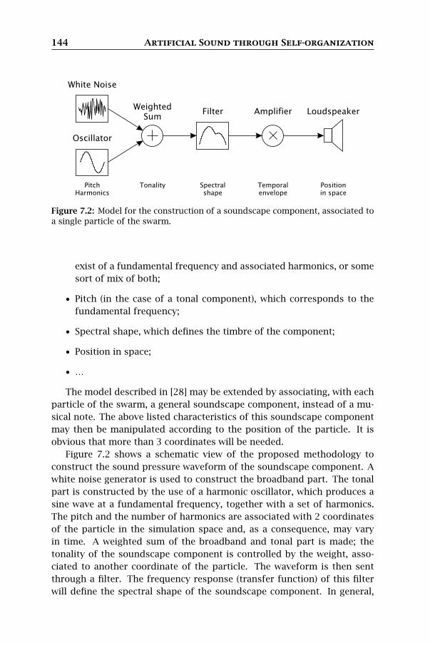
144 Artificial Sound through Self-organization
LoudspeakerAmplifierFilterWeighted
Sum
Oscillator
White Noise
Positionin space
Temporalenvelope
Spectralshape
TonalityPitchHarmonics
Figure 7.2: Model for the construction of a soundscape component, associated toa single particle of the swarm.
exist of a fundamental frequency and associated harmonics, or some
sort of mix of both;
• Pitch (in the case of a tonal component), which corresponds to the
fundamental frequency;
• Spectral shape, which defines the timbre of the component;
• Position in space;
• …
The model described in [28] may be extended by associating, with each
particle of the swarm, a general soundscape component, instead of a mu-
sical note. The above listed characteristics of this soundscape component
may then be manipulated according to the position of the particle. It is
obvious that more than 3 coordinates will be needed.
Figure 7.2 shows a schematic view of the proposed methodology to
construct the sound pressure waveform of the soundscape component. A
white noise generator is used to construct the broadband part. The tonal
part is constructed by the use of a harmonic oscillator, which produces a
sine wave at a fundamental frequency, together with a set of harmonics.
The pitch and the number of harmonics are associated with 2 coordinates
of the particle in the simulation space and, as a consequence, may vary
in time. A weighted sum of the broadband and tonal part is made; the
tonality of the soundscape component is controlled by the weight, asso-
ciated to another coordinate of the particle. The waveform is then sent
through a filter. The frequency response (transfer function) of this filter
will define the spectral shape of the soundscape component. In general,

7.4 Soundscape selection using genetic algorithms 145
the frequency response is characterized by several parameters, say n. For
example, if a band-pass filter is used, then n = 2 (low and high cutoff
frequency). Thus, n particle coordinates may be associated to this filter.
Subsequently, the waveform is amplified. By varying the amplification fac-
tor according to a coordinate of the particle, the temporal envelope of the
soundscape component is constructed. Finally, the amplified waveform is
sent to a (virtual) loudspeaker. The spatial position of this loudspeaker,
relative to the listener, is characterized by 3 (spherical) coordinates. This
position may also be varied according to 3 coordinates of the particle in the
simulation space. The proposed methodology thus requires that a particle
swarm is simulated in a hyperspace of D = n+ 7 dimensions.
7.4 Soundscape selection using genetic algorithms
From the discussion in Sections 7.2.4 and 7.3, it is clear that an artificial
soundscape produced with our model will be very flexible according to its
spectral and temporal structure, but also that this flexibility comes with
the cost of a large number of free parameters. As already mentioned in
the introduction of this chapter, it would be hard for a test person to tune
these parameters to achieve a suitable soundscape to a given environment.
Moreover, several of these parameters will be hard to grasp for a lay test
person.
Therefore, it would be best if the test person does not have to tune
these parameters at all, but only has to answer simple questions, such as
deciding which of two soundscapes fits best to a given environment. The
parameters could then be optimized automatically. In this work, it was
chosen to use an interactive genetic algorithm for this purpose. In the
next sections we will introduce the basic ideas, and we will outline the
methodology implemented in our model.
7.4.1 Background and basic algorithm
Genetic algorithms (ga) were introduced by John H. Holland [145] for solv-
ing optimization problems. They are based on the principles of biologi-
cal evolution, which were for the first time formulated by Charles Darwin.
Earlier research on optimization methods inspired by evolution theory had
resulted in methodologies called evolutionary programming and evolution
strategies. Because of the similarities between these different approaches,
they have been mixed frequently, which led to a new field of research called
evolutionary computing (ec) [5, 89], a subfield of ai. ec techniques are ro-
bust, but however do not guarantee that the global optimum will be found.

146 Artificial Sound through Self-organization
Modern evolutionary synthesis, which refers to the integration of both
Charles Darwin’s theory of the evolution of species and Gregor Mendel’s
theory of genetics, is mainly based on the following biological principles [5,
324]:
Structure and behaviour: Individuals can be viewed as a duality of their
genotype, the underlying genetic coding, and their phenotype, their
behaviour, psychology and morphology [111].
Natural selection: The individuals best adapted to their environment have
the most chance to survive and reproduce. A well adapted individ-
ual has an appropriate phenotype in light of its environment, and is
said to have a high fitness degree. The goal of natural selection is to
maintain or increase the fitness of the population.
Heredity: Genes are the transfer units of heredity. The collection of all
genes is called the genome, and represents the genotype of an individ-
ual. High fitness individuals that are capable to reproduce, transfer
(part of) their genetic information into the next generation. During
reproduction, the genes of the parents are recombined. Errors are in-
evitable during this reshuffle of information, which lead to mutational
variation.
The above principles of evolution are simulated by the following general
ec algorithm to solve optimization problems [5, 324]:
1. An initial population of random individuals is created, represented
by their genetic information (genes). Each individual represents a
possible solution to the optimization problem.
2. The following loop is repeated until a termination condition is satis-
fied:
(a) The fitness of each individual of the population is evaluated,
which represents the quality of the individual as a solution to
the problem.
(b) The following genetic operators are randomly applied to form a
new generation:
Selection: Two individuals of the population are selected, with
a probability based on their fitness score. The higher their
fitness, the more chance they have to be selected for repro-
duction;
Crossover: Two new individuals (offspring) are created by ran-
dom recombination of the genomes of the selected individ-
uals (parents);
7.4 Soundscape selection using genetic algorithms 147
Mutation: A randomly chosen gene of the offspring is altered
with a certain probability.
3. The best solution in the final population (individual with highest fit-
ness score) is considered as the solution to the optimization problem.
This may be the optimal solution, or an approximate solution.
In the following sections, we will discuss the different steps of the gen-
eral algorithm more in detail. The particular problems associated with its
use in the process of artificial soundscape selection will receive special
attention.
7.4.2 Representation
In this work, the individuals of a population are single artificial sound-
scapes (phenotype). The genotype of an artificial soundscape considered
is formed by the parameters discussed in Section 7.2.4. A good choice for
the data structure to represent this genotype is important. It has to be
minimal, but also completely expressive: all possible solutions should be
representable with the chosen data structure. A large number of possibili-
ties have been used in the past, such as strings of bits (typical for a ga) or
tree structures. The choice of representation will obviously influence the
operators that may act on the genome.
A complication is that the number of parameters may vary between
individuals. The number of swarm, particle and soc related parameters is
fixed; however, the number of attractors may vary. Note that the number
of parameters associated with a single attractor is also fixed — the swarm
location is described byD coordinates, andD is defined by the structure of
the sound production model, which is considered fixed. Thus, it is natural
to consider a genome as consisting of a variable number of fixed length
segments. The first segment is always present, and contains the swarm,
particle and soc related parameters. Each (optional) subsequent segment
contains the parameters for an attractor. The parameters within a single
segment are coded as an array of (integer) values, which is one of the most
simple data structures to code a genome. Each element in the array is then
called a gene. The direct representation of the genome using integer values
is derived from the evolution strategy technique.
7.4.3 Interactive evaluation of fitness
With each individual, represented by its genome, a fitness score is asso-
ciated. In general optimization problems, this fitness score is calculated

148 Artificial Sound through Self-organization
by a fitness function or objective function. The fitness score expresses the
quality of the solution in the optimization problem. In our case, the fit-
ness of a soundscape represents the degree to which the soundscape fits
to the given environment. It is obvious that this fitness value can not be
calculated according to a formula — this has to be decided by a human
listener.
ec techniques that require some human input for fitness evaluation are
commonly referred to as interactive evolutionary computation (iec) algo-
rithms [304, 355]. iec techniques are mainly used in the field of image
processing and computer graphics [292], e.g. it has been applied to face
recognition of criminal suspects [52]. iec algorithms have also been used
succesfully to create artificial music [224, 225, 313].
Because human interaction is required, some issues are involved with
iec. Human fatigue is reported by many researchers as the limiting fac-
tor for the number of evaluations by one user [304]. In addition, human
evaluations are slow and expensive, as compared to fitness function com-
putation. Moreover, soundscapes may not be presented in parallel, as is
the case with images, and have to be listened to for a certain duration
(e.g. at least one minute if the temporal structure has to be evaluated).
iec techniques therefore often employ only small populations to reduce
the number of evaluations required, and employ ga implementations that
converge relatively fast with small populations. Implementations that are
able to accept evaluations from many users (concurrently) may overcome
these limitations.
Next to this, finding “the best fitting soundscape” for a given environ-
ment is a subjective matter. For the proposed model for selection of the
most suitable soundscape to work, we have to accept the hypothesis that
the underlying spectral and temporal characteristics of the most suitable
soundscape will be about the same for most people. Nevertheless, the eval-
uation of a single soundscape may vary between users. To reduce the effect
of this variation (= noise), it is important to make the task for the user as
simple as possible. It is rather hard for a user to rate a soundscape with
a fitness value. On the other hand, comparing a small number of sound-
scapes for fitness is relatively easy. A ranking system therefore seems
suitable, in which the individual soundscapes of a population are sorted
according to their matching qualities to a given environment, by the use of
simple comparisons (the user has to choose the most suitable soundscape
out of several). The fitness value may then be a function of the position
of the soundscape in the final ranking. Another option is to have the fitter
fraction of the population reproduce and not the less fit fraction of the
population.

7.4 Soundscape selection using genetic algorithms 149
7.4.4 Selection
When all individuals of the population have been evaluated for their fitness,
the selection mechanism has to choose the individuals for recombination,
or in other words, the parents that will have to produce offsprings. The
purpose of the selection operator is to direct the search towards individu-
als that perform well. Search and optimization algorithms always have to
make a compromise between exploitation (the extent to which the search
is directed by the discovery of fairly good solutions) and exploration (the
attention of the algorithm to unknown regions of the search space). In
ec algorithms, the exploitation is done by selection and crossover, while
mutation takes care of the exploration part. This compromise is character-
ized by the selection pressure of the algorithm, which among other things is
influenced by the fraction of individuals of the population selected to pro-
duce a new population. The selection pressure will have a large influence
on the number of iterations needed for the algorithm to converge.
Two types of selection algorithms exist: generational and incremental
selection. In a generational selection mechanism, the offspring will form
the new generation. These methods may be extended with elitism: the in-
dividual with the highest fitness score is then automatically transferred
to the next generation. This way it is ensured that the best individual
encountered always makes part of the population. In an incremental selec-
tion algorithm, parents and offspring compete with each other to produce
a new generation. This implies that elitism is always present in this type
of selection strategy.
The following selection schemes are the most commonly encountered
in literature [5, 324]:
Uniform: A new generation is produced, in which each individual of the
old generation has the same probability of being chosen.
Roulette wheel: In this selection method, individuals are chosen with a
chance based on the magnitude of their fitness score, relative to the
total fitness of the population. The higher the fitness score, the more
likely an individual will be selected. The name is derived from the
analogy with a biased roulette wheel, where each individual is as-
signed a slot sized in proportion to its fitness.
Tournament: A number of individuals are chosen using another selection
strategy (e.g. roulette wheel or uniform). The best individual from
this group is then selected as the winner of the tournament. For each
individual of the new generation, a tournament is held.

150 Artificial Sound through Self-organization
(λ, µ): This selection method stems from evolution strategies. From the
total population, the subset of µ individuals with highest fitness score
is selected, called the parent population. This subset is allowed to
produce an offspring population consisting of λ individuals. (λ, µ)
selection is similar to the roulette wheel strategy, but here the best µ
individuals are given a chance 1/µ, while the other individuals have
no chance to reproduce.
(λ + µ): This strategy is an incremental variation of (λ, µ) selection, with
the difference that a new generation is produced by chosing the best
µ individuals from the union of µ parents and λ children. An inter-
mediary generation thus consists of λ+ µ individuals.
The above list is sorted from lowest selection pressure to highest se-
lection pressure. To reduce the number of tests needed to find a suitable
soundscape, an algorithm with high selection pressure is prefered. Another
advantage of (λ, µ) selection is that the exact fitness value of each individ-
ual (soundscape) does not have to be known — only the µ best individuals
have to be identified. Incremental selection strategies have the disadvan-
tage that their selection pressure is very sensitive to noise in the fitness
evaluation, which makes them less suitable for use in an iec. Therefore,
(λ, µ) selection was chosen in our implementation.
7.4.5 Crossover and mutation
The genetic operators used in ec are crossover and mutation. Crossover
recombines the genetic information of two parents to produce two children.
Its main purpose is to preserve the genes of well adapted individuals in
the next generations. The mutation is executed on a single genome, with
a smaller probability than crossover. Its main purpose is to create new
genetic information and to keep a certain amount of genetic diversity in
the population.
The choice of the crossover and mutation operators largely depends on
the adopted representation of the genome. When this representation is a
simple array, the following crossover operations are common [5, 324]:
One point crossover: The genome of both parents is cut in two pieces at
the same randomly chosen location, and the parts are swapped.
Two point crossover: Two points are randomly selected along the genome
and the parts in between these two points are swapped.
Uniform crossover: Two children are created by randomly choosing each
gene from either parent.

7.4 Soundscape selection using genetic algorithms 151
In our model, each genome consists of a variable number (at least 1)
of fixed length segments. It seems therefore natural to use 2 types of
crossover operators: one type acting on the internal genes of segments
(intra-segment), and another type acting on the genome as a succession of
segments (inter-segment). The following specialized crossover operators
were conceived for our particular representation:
Uniform intra-segment crossover: A random segment of the first parent
is chosen. If this is the first segment of the genome (containing the
swarm, particle and soc related parameters), the first segment of the
second parent is also selected; otherwise, a random segment of the
second parent is selected (not the first). A uniform crossover is then
performed with the genes from both segments, producing 2 children.
Linear intra-segment crossover: The same algorithm is applied to select
2 segments from both parents. However, instead of randomly swap-
ping genes, the offspring genes are chosen randomly somewhere in
between the corresponding gene values of the parents (arithmetic re-
combination [89]). This type of crossover produces only a single off-
spring, and therefore has to be applied twice.
Inter-segment crossover: This is a type of one point crossover operator,
in which the swapping location may only be chosen on the borders
between segments. Segments are recombined, and genomes may have
a different length.
The mutation operator usually performs some small, random pertur-
bations to genes with a rather small probability. When an individual is
represented as a bit string, the mutation commonly takes the form of a bit
flip operation. The mutation of real values often consists of modifications
according to a Gaussian distribution with a specified standard deviation.
Again, an operator acting on genes of segments and an operator acting on
the genome as a succession of segments was implemented:
Gene mutation: A random gene is altered by adding a stochastic value with
a Gaussian distribution.
Segment addition: A segment consisting of random genes, representing
the parameters of an attractor, is added at a random location after
the first segment.
Segment deletion: A random segment is removed (not the first one).
An illustration of all crossover and mutation operators described is
shown in Figure 7.3.

152 Artificial Sound through Self-organization
segment additionsegment deletiongene mutation
inter–segment crossoverlinear intra–segment crossover
uniform intra–segment crossover
uniform crossovertwo point crossoverone point crossover
Figure 7.3: Genetic crossover and mutation operators.
7.5 Implementation and performance
The model to produce and assess artificial soundscapes, outlined in the
previous sections, is called SwarmScape. In this final section, we will give
a concise overview of the most important implementation issues, together
with some preliminary performance results.
7.5.1 Soundscape generation
The particle swarm and artificial soundscape generation algorithms have
been implemented as a stand-alone program written in C++, according
to the description in Sections 7.2 and 7.3. However, several design pat-
terns [115] have been applied to create a large flexibility for the user. A
configuration xml input file describes the algorithm for the construction
of a soundscape component associated to a single particle. The schema of
Figure 7.2 may be used, but it is also possible to remove steps, or to add
new steps (filters, noise generators, oscillators…) to the chain, in an arbi-
trary sequence. The required dimension of the swarm simulation space is
7.5 Implementation and performance 153
calculated automatically. The swarm algorithm parameters (Section 7.2.4)
are loaded from a genome xml input file.
The sound pressure waveform associated to each component of the
artificial soundscape is modeled as a stream of audio samples. A general iir
digital filter was implemented, which is described by the following standard
difference equation [262]:
a0yi = +b0xi +· · · +bnbxi−nb−a1yi−1 −· · · −anayi−na
(7.9)
where xi and yi represent resp. the input and output stream of audio sam-
ples. The frequency response of this filter is defined byn = na+nb+2 filter
coefficients, which may be large (> 4) for most useful filters. Three special
cases were implemented, in which the filter coefficients are automatically
calculated based on a small number of more intuitive frequency response
parameters (see e.g. [262] for a more elaborate explanation of these filter
types):
Butterworth low-pass filter (n = 1): Only the cutoff frequency has to be
supplied by a particle coordinate;
Butterworth band-pass filter (n = 2): Only the low and high frequency
cutoff frequency have to be supplied;
Biquadratic filter (n = 4): This is a 2nd order band-pass filter with 2 ze-
ros and 2 poles. Particle coordinates (angle and radius) for the loca-
tions of the zero and pole in the upper half of the z-plane have to be
supplied.
The swarm may be updated for each sample produced, but to reduce
the computational burden, it is a better idea to update the swarm at a lower
rate. It was found that an update each 10 ms (corresponding to 441 sam-
ples at a sample rate of 44.1 kHz) does not introduce noticeable glitches.
The 3D positioning of the different soundscape components for headphone
listening is done using the fmod library [110], which implements the hrtf
functions of a standard human listener. Using a modern pc equiped with
a good quality sound card, it is easily possible to simulate the soundscape
produced by a swarm of 10 particles or more in real time, which is suffi-
cient to imitate a wide range of soundscapes. The audio may furthermore
be encoded automatically to the (lossy) audio format Ogg Vorbis [242], to
enable (online) streaming to an evaluation client.
In addition to the main soundscape generation program, a graphical
interface was implemented [81], which makes it possible to study the in-
fluence of the swarm algorithm parameters relatively easily. It was found
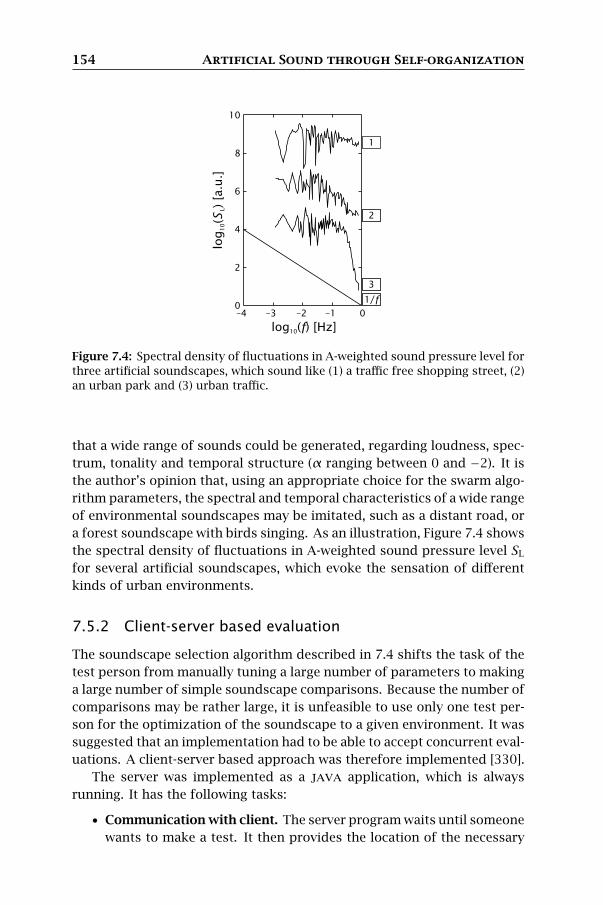
154 Artificial Sound through Self-organization
2
1
1/f
3
10
8
6
4
2
0–2 –1 0–3–4
log
()
[a.u
.]10
LS
log ( ) [Hz]10 f
Figure 7.4: Spectral density of fluctuations in A-weighted sound pressure level forthree artificial soundscapes, which sound like (1) a traffic free shopping street, (2)an urban park and (3) urban traffic.
that a wide range of sounds could be generated, regarding loudness, spec-
trum, tonality and temporal structure (α ranging between 0 and −2). It is
the author’s opinion that, using an appropriate choice for the swarm algo-
rithm parameters, the spectral and temporal characteristics of a wide range
of environmental soundscapes may be imitated, such as a distant road, or
a forest soundscape with birds singing. As an illustration, Figure 7.4 shows
the spectral density of fluctuations in A-weighted sound pressure level SL
for several artificial soundscapes, which evoke the sensation of different
kinds of urban environments.
7.5.2 Client-server based evaluation
The soundscape selection algorithm described in 7.4 shifts the task of the
test person from manually tuning a large number of parameters to making
a large number of simple soundscape comparisons. Because the number of
comparisons may be rather large, it is unfeasible to use only one test per-
son for the optimization of the soundscape to a given environment. It was
suggested that an implementation had to be able to accept concurrent eval-
uations. A client-server based approach was therefore implemented [330].
The server was implemented as a java application, which is always
running. It has the following tasks:
• Communication with client. The server program waits until someone
wants to make a test. It then provides the location of the necessary

7.5 Implementation and performance 155
data (sounds, images etc.) for the client to perform a test. Since
(λ, µ) selection extended with elitism is used, the knowledge of the
subset of µ best individuals from the population is required, together
with the best individual. This subset is estimated using a method in-
spired by the final stage of the world championship soccer. Firstly, a
group stage is held, in which the soundscapes are randomly divided
into groups of 4. In this case, a test consists of asking the person to
select the 2 most suitable soundscapes out of 4. As a consequence
it is required that λ = 2µ. Secondly, a stage with immediate elimi-
nation is held with the selected soundscapes, to determine the best
soundscape, which automatically is transferred to the next genera-
tion. In this case, a test consists of asking the person to select the
most suitable soundscape out of 2. The evaluation of one generation
thus requires λ/4+µ−1 or 34λ−1 tests, in which at least 2λ−2 times
a soundscape has to be listened to.
• Genetic algorithm execution. The server keeps track of the tests
to be made, those already performed, their results, and the tests in
progress. When the subset of µ most suitable soundscapes is known,
the server executes the genetic algorithm, at which a new generation
is calculated. The author found no ga libraries capable of handling
genomes subdivided into segments, so a specialized ga as described
in Section 7.4 was implemented from scratch. For each new genera-
tion, artificial soundscapes associated with the genomes in the popu-
lation are created. Finally, the most suitable soundscape is identified
as the best individual of the population when a predefined number
of generations have been calculated.
The client was implemented as a signed java applet, which may be
evoked at all times via a html page. Different clients may run continuously,
which enables an internet-based evaluation. The client requires a browser,
the java runtime environment, and an audio card with headphone, to be
able to make a test. Once the client is started, it will make a connection with
the server, and download the necessary data to perform a test (soundscapes
and image). Figure 7.5 shows an example of a test, in which the most
suitable soundscape out of 2 has to be chosen.
7.5.3 Convergence speed
Some preliminary tests were performed to make an estimation of the con-
vergence speed. For this purpose, a set of standard objective functions
were applied to the soundscape genomes, replacing the human evaluation
of the soundscapes. A mathematical description of the test functions as
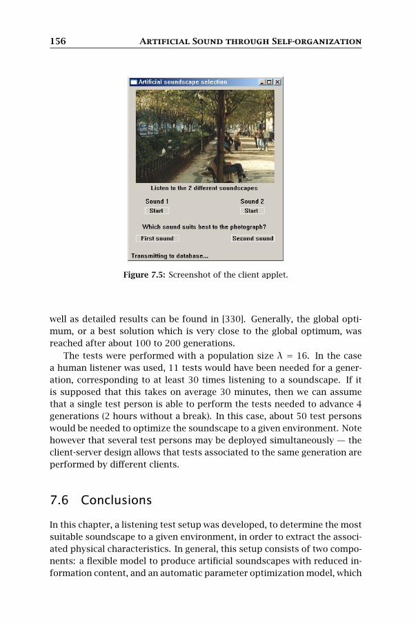
156 Artificial Sound through Self-organization
Figure 7.5: Screenshot of the client applet.
well as detailed results can be found in [330]. Generally, the global opti-
mum, or a best solution which is very close to the global optimum, was
reached after about 100 to 200 generations.
The tests were performed with a population size λ = 16. In the case
a human listener was used, 11 tests would have been needed for a gener-
ation, corresponding to at least 30 times listening to a soundscape. If it
is supposed that this takes on average 30 minutes, then we can assume
that a single test person is able to perform the tests needed to advance 4
generations (2 hours without a break). In this case, about 50 test persons
would be needed to optimize the soundscape to a given environment. Note
however that several test persons may be deployed simultaneously — the
client-server design allows that tests associated to the same generation are
performed by different clients.
7.6 Conclusions
In this chapter, a listening test setup was developed, to determine the most
suitable soundscape to a given environment, in order to extract the associ-
ated physical characteristics. In general, this setup consists of two compo-
nents: a flexible model to produce artificial soundscapes with reduced in-
formation content, and an automatic parameter optimization model, which

7.6 Conclusions 157
is based on the response of the test person. The test setup was imple-
mented in a client-server based framework.
For the production of artificial soundscapes, a method based on swarm
intelligence techniques was chosen, because a strong link can be drawn
between this method and dynamic systems in which complexity may arise.
Compared to using (manipulated) recordings, a much larger flexibility can
be achieved, which however has to be limited somewhat for listening tests.
In order to optimize the swarm model parameters, a hand tailored ga is
deployed, because the search space may have multiple local minima, and
because the swarm model parameters have a strong non-linear influence on
soundscape suitability. In addition, the interactive soundscape suitability
evaluation by the test person introduces noise. This is a major problem
with most search algorithms and restricts the choice of algorithm. Due to
the noise introduced by the test person, little or no benefit can be achieved
by using a hybrid method (e.g. a memetic algorithm [134]) for optimization
in the neighbourhood of a local solution.
Due to a lack of time, the listening test setup discussed in this chapter
has not been applied on a large scale in the framework of this Ph. D. Some
small scale tests have been carried out, which demonstrated the proper
operation of the various components of the setup, and the feasibility to
conduct listening tests via the internet. However, to be able to link physi-
cal soundscape characteristics with context-based soundscape preference,
more research will be needed.


Part IIIAssessment of Quiet Areas


Chapter8
Quiet Areas
8.1 Introduction
In this part, we will consider a particular type of environment: the quiet
area (qa). A quiet area generally is defined as an area that is more quiet
than the surrounding region, and which has a psychological restoring ef-
fect [354] on people visiting it. Quiet areas may be urban as well as rural.
Due to the increasing influence of traffic and industrialization on our sonic
environment, quiet places become more and more scarce. There is a grow-
ing awareness that quiet areas deserve special attention and preservation.
In the ec environmental noise directive [93] and in policy intentions of
many countries, the preservation and management of quiet areas (urban
as well as rural) has therefore been subscribed.
It has to be noted that qa preservation is not synonymous with nature
preservation — the aim is not to guarantee high quality biotopes for ani-
mals. In many cases, nature will be prominently present in a quiet area,
but it is not the goal on itself. Also, a qa is not the same as a quiet living
environment. People visiting quiet areas to escape from the noise of daily
life, may have their attention more focused on the environment. The em-
phasis therefore lies on the visual as well as the auditive perception of the
visitor, engaging in mainly recreational outdoor activities.
8.2 Perception of quietness
The quiet area obviously is (or at least should be) experienced as quiet by
the average listener. However, in this context, quietness does not mean
a complete absence of sound (= silence), but rather the absence of “dis-
turbing” sound. The energy equivalent sound pressure level is therefore

162 Quiet Areas
Perception
Influence on
quiet soundscape
ConsciousRecognitionAssociation
UnconsciousHolistic
AccentuationDisturbance
Basic qualitySilence
Sound eventsBackground
Soundscape
Figure 8.1: Various aspects related to a soundscape.
less suited as the only indicator to characterize quiet areas and possibly to
grant quality labels. An acoustic ecology approach may be more appropri-
ate; although the soundscape concept has been discussed in the context
of noise annoyance (e.g. see [285, 193, 175]), sleep disturbance [245] and
health effects [192, 293], its main advantage lies in the study of the sonic
environment of urban parks or squares and natural or rural areas [356]. In
line with Schafer’s vision, the soundscape can be considered as the super-
position of an always present background (the keynote sound) and sound
events (signals, soundmarks…). This subdivision is illustrated in Figure 8.1.
The background or ambient largely determines the overall feeling of
quietness, and thus the basic quality of the quiet soundscape — it de-
termines whether it is considered silent or not. This background can be
heard, but the hypothesis is that it does not trigger much meaning since it
will probably not be listened to consciously. Events can disturb the sound-
scape, but it is also possible that they accentuate the basic quality (e.g. an
occasional bird sound). It is known that the perception of noise events —
and possibly also the resulting annoyance — involves source recognition
and associations to the effect the source has on the relationship between
person and environment [203]. The background, on the other hand, may
not lead to any source recognition; it may be experienced in a more holistic
way, having a more direct effect on general well-being.
A suitable soundscape for a quiet area implies that the background
arouses a perception of silence, which implies that the ambient noise level
is relatively low. A small number of events may be perceived as occasional

8.3 Towards a multi-criteria approach 163
disturbances. When too many disturbances are present, the soundscape
may loose its feeling of quietness. However, natural or location typical
noise events may accentuate quietness, rather than to jeopardize it. Fur-
thermore, in order to arouse a perception of silence, it may be necessary
that the spectral and temporal structure of the soundscape (background
and sound events) contributes to a relaxing feeling, and that non-acoustic
factors such as the ecologic and scenic value of the area should come up
to the visitor’s expectations.
8.3 Towards a multi-criteria approach
Based on the above considerations, it is clear that a soundscape approach
to quiet area quality is appropriate. Many have stressed that soundscape
quality cannot simply be assessed by studying a single noise level indica-
tor. In [49], laboratory experiments are used to investigate the effect of
relative levels of natural background noise and different intruding sounds
on quality perception of the intruding sound. It is found that, next to the
overall level, a physical indicator for noticeability is needed to explain the
results. The extensive overview report by Symonds [302] mentions several
interesting approaches to quality assessment that were proposed and/or
used in European countries, but nevertheless concludes on a single indica-
tor based on overall level. In [106], it is argued that since the ambient noise
level is low, intrusive noises are more audible and man-made sounds will
more likely be intermittent and variable in level and duration. This makes
the use of long term time-average sound pressure levels such as Lden less
suitable. Event noise level (measured relative to the background level) and
duration were found to be uncorrelated by Miller [220], when he quantified
noise intrusions in National Parks in the us, which means that both add
information about a location. Much the same approach was used in [317]
to assess non-natural noise intrusions in Dutch quiet areas.
In [10], it is proposed to go beyond the use of quantitative approaches
using the energy equivalent sound pressure level, when qualifying urban
sound environments with a more complex temporal structure, or during
quiet periods. Counting the number of noise events, using statistical levels
or using psychoacoustic criteria is discussed. Brown [50] even proposes to
depart from the classical level based approach and to adopt criteria based
on the information content of sounds for outdoor soundscapes, e.g. “mov-
ing water should be the dominant sound”. In [238] urban and suburban
green areas are investigated in an extensive study. The author neverthe-
less also concludes on a threshold for LAeq as a physical criterion.

164 Quiet Areas
Overall, two lines can be discovered in current research on quiet area
soundscapes. One line pursues the scientific goal of trying to understand
the influence of the soundscape on its visitor’s state of mind. It consistently
leads to the conclusion that long term time-average sound pressure levels
are poor indicators. A second line of research has started from classical
noise mapping and suggests additional indicators, albeit mainly noise level
based. In the next chapter, we propose to combine the best of both worlds
in a multi-criterion assessment. Nevertheless the aim is to arrive at a set
of indicators with strong focus on applicability.

Chapter9
The Quiet Rural Soundscape
and How to Characterize It
B. De Coensel and D. Botteldooren
Published in Acta Acustica united with Acustica 92(6):887–897, 2006.
« « «
In this chapter, the quiet rural area is studied from a soundscape
perspective, and a multi-criteria approach for quality assessment is
proposed. Part of this work has been sponsored by the Flemish envi-
ronmental administration (aminabel). Results of this research were
presented at the 6th European Conference on Noise Control [36].
9.1 Introduction
The concept of quiet area (qa) has been introduced in many countries’
legislation and is more recently mentioned explicitly in the European Envi-
ronmental Noise Directive [93]. This document defines: “Quiet area in an
agglomeration” shall mean an area, delimited by the competent authority,
for instance which is not exposed to a value of Lden or of another appropri-
ate noise indicator greater than a certain value set by the Member State,
from any noise source. Similarly: “Quiet area in open country” shall mean
an area, delimited by the competent authority, that is undisturbed by noise
from traffic, industry or recreational activities. These definitions leave room
for interpretation and critical reflection. The aim of this paper is to provide
a starting point for this.
Since quiet areas are nothing but soundscapes which have the particular
quality of quietness, it is worthwhile to bring the discussion on quiet area
166 The Quiet Rural Soundscape
characterization, categorization, and quality labeling to the broader per-
spective of soundscape research. This work nevertheless focuses on the
very particular context sketched in Section 9.2.1: the quiet area in open
country.
The study of soundscapes in general and quiet areas in particular can
serve different purposes. Most of recent research [356] aims at scientific
understanding from a psychological or sociological point of view. In policy
planning, policy support, monitoring, and environmental impact assess-
ment, indicators are commonly used. This chapter looks in particular at
indicators for characterizing the quiet rural soundscape. Deriving such in-
dicators involves a delicate balance between scientific accuracy and prac-
tical applicability. Indicators should fulfill the general requirements for a
good indicator (as proposed e.g. by the oecd): there should be a scientifi-
cally proven link between the effect one wants to quantify and the indicator;
the indicator should be measurable at reasonable cost and preferably cal-
culation models should be available; the indicator must be understandable
by policy makers and the population at large. In addition, indicator-sets
should highlight non-overlapping dimensions of the problem.
In Section 9.2 we try to fulfill the first requirement: scientifically proven
link between effect and indicator, mainly on the basis of an extended liter-
ature study. This literature study mainly focuses on soundscape research
but also (mental) health related aspects are discussed. In Section 9.3 the
shortlist of possibly useful indicators is concretized, taking into account
measurability, predictability and understandability for a broad public. The
indicators are tested on a typical quiet rural soundscape and for compar-
ison also on an urban area with particular focus on the non-overlap re-
quirement. This section thus aims at proving that the selected indicator-
set fulfills the additional requirements outlined in the previous paragraph.
Section 9.4 discusses our findings and proposes a multi-criteria assessment
of quiet rural soundscape quality.
9.2 Quiet areas from a soundscape perspective
9.2.1 Defining the context
The soundscape concept has been introduced into the research of urban
acoustic environments a few decades ago from an artistic angle [312, 280].
Since then, several authors have used the concept — but unfortunately
also sometimes misused it — in their research on urban and rural sound
fields, its perception and its effect on quality of life, wellbeing, and health.
A comprehensive literature overview can be found in [356, 193]. As the

9.2 Quiet areas from a soundscape perspective 167
name suggests, soundscapes have much in common with landscapes. Both
combine physical characteristics with perception in a particular context
and from a particular point of view. Studying them can lead to preservation
of unique specimens or to the design of pleasing new ones. A quiet area
can be regarded as a particular type of soundscape that is worth preserving
because of a unique feature: quietness. Preserving a qa is as such not
necessarily different from preserving other (typical) soundscapes. Hence
we will from this point on refer to the quiet rural soundscape as the object
of this study.
It has been stressed by many that a soundscape is always assessed
within a context and that non-acoustical factors play an important role
[109, 163]. These non-acoustical factors can be related to the physical
environment (called the “enviroscape”), such as the visual setting or the
presence of air pollution, or to personal factors (called the “psychscape”),
such as noise sensitivity and attitude toward the noise source [164]. The
term “psychscape” is used here in a slightly generalized form including the
instantaneous state of mind. In this paper, the context is well-defined:
• The “enviroscape” is a rural one: combined agriculture and woodland,
bushes, scattered farms and an occasional village, a small stream or
other water features, low level roads and paths without or with very
limited motorized traffic. Occasionally some infrastructure for quiet
recreation such as horseback riding, cycling, sailing…
• The “psychscape” is the state of mind of people looking for quiet
recreation, relaxation, quality time and mental restoration. In a small
survey with visitors to a typical quiet rural area, enjoying landscape
and nature, walking and cycling (physical exercise), enjoying the si-
lence, relaxing, and studying plants and animals, were mentioned as
important reasons for being in this area.
This context may look very limited in scope but it is of importance for
many European city dwellers because it is within reach for “a day at the
countryside” in most places. The great outdoors and large natural reserves
are not reachable without travelling the better part of a day and thus have
to be left for holiday periods.
9.2.2 Verbal descriptors
Reported work related to finding verbal descriptors for categorizing sound-
scapes differs strongly between holistic evaluations or event oriented eval-
uation. In [266] Raimbault et al. analyse lexical categories of wording used
by both city planners and city-users in open interviews. They come to

168 The Quiet Rural Soundscape
the conclusion that city-users tend to use most often “vocabulary of com-
parison” (noises, “noise of source” object, subject pronouns, assessment),
“generic expressions” (noise, descriptions of spaciousness, descriptions of
duration), and “human noises descriptions” (human voices, subject pro-
nouns, assessment), in that order. This confirms the finding from ear-
lier work that description of a soundscape includes components related to
sounds or noises that are mainly linked to sources and components related
to ambient or background sound [104]. In the quiet rural soundscape, the
ambient or background noise becomes more important for several reasons.
Long periods filled with a mixture of sounds will separate noises that can
clearly be linked to specific sources. We have previously [36] put forward
the hypothesis that a feeling of quietness is determined by intervals of si-
lence where silence itself is defined as the ambiance of a soundscape, the
gap or distance, the auditory space between sound events.
For an assessment of soundscapes, most researchers use a semantic
differential (sd) [268, 3, 325, 172, 322, 349, 117, 171, 20]. As an indica-
tor, the sd has properties that are of particular interest: measurability at
reasonable cost, transparency for policy makers and the public at large.
Moreover, it allows to force those questioned to assess the soundscape in
a more holistic way and to go beyond the identification and description
of sound sources. The words used often involve emotional reaction and
feeling related to the acoustic field. As a scientific tool, open question-
naires yield much more valuable information. The analysis of the above
mentioned field studies revealed principle components in the assessment
of soundscapes. Although there are discrepancies between studies, Ta-
ble 9.1 shows that at least some broad lines emerge. Discrepancies are not
only attributable to the different use of wording but also to the range of
soundscapes considered. A first factor, which seems to arise as the most
important factor in all studies considered, is related to the pleasantness
or loudness of the soundscape. A second factor is related to the temporal
structure, the eventfulness or the activity of the soundscape. Next to these,
a factor related to the familiarity with or the auditory expectation of the
soundscape is often encountered [3, 325, 172], as well as a factor related to
the spatial characteristics of the soundscape [268, 322] and a factor related
to the spectrum or timbre of the soundscape [349].
9.2.3 Physical indicators
Based on the research results summarized in Table 9.1, the sound strength
is recognized as an important factor. A classical noise level indicator seems
well suited to describe this first factor in the soundscape. However, this
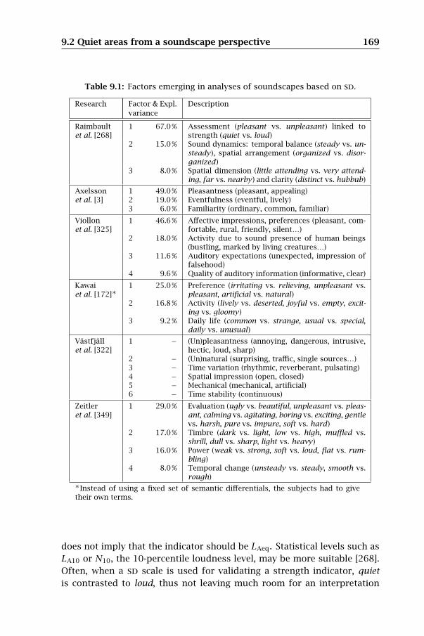
9.2 Quiet areas from a soundscape perspective 169
Table 9.1: Factors emerging in analyses of soundscapes based on sd.
Research Factor & Expl. Descriptionvariance
Raimbaultet al. [268]
1 67.0 % Assessment (pleasant vs. unpleasant ) linked tostrength (quiet vs. loud)
2 15.0 % Sound dynamics: temporal balance (steady vs. un-steady), spatial arrangement (organized vs. disor-ganized)
3 8.0 % Spatial dimension (little attending vs. very attend-ing, far vs. nearby) and clarity (distinct vs. hubbub)
Axelsson 1 49.0 % Pleasantness (pleasant, appealing)et al. [3] 2 19.0 % Eventfulness (eventful, lively)
3 6.0 % Familiarity (ordinary, common, familiar)
Viollonet al. [325]
1 46.6 % Affective impressions, preferences (pleasant, com-fortable, rural, friendly, silent…)
2 18.0 % Activity due to sound presence of human beings(bustling, marked by living creatures…)
3 11.6 % Auditory expectations (unexpected, impression offalsehood)
4 9.6 % Quality of auditory information (informative, clear)
Kawaiet al. [172]∗
1 25.0 % Preference (irritating vs. relieving, unpleasant vs.pleasant, artificial vs. natural)
2 16.8 % Activity (lively vs. deserted, joyful vs. empty, excit-ing vs. gloomy)
3 9.2 % Daily life (common vs. strange, usual vs. special,daily vs. unusual)
Vastfjallet al. [322]
1 − (Un)pleasantness (annoying, dangerous, intrusive,hectic, loud, sharp)
2 − (Un)natural (surprising, traffic, single sources…)3 − Time variation (rhythmic, reverberant, pulsating)4 − Spatial impression (open, closed)5 − Mechanical (mechanical, artificial)6 − Time stability (continuous)
Zeitleret al. [349]
1 29.0 % Evaluation (ugly vs. beautiful, unpleasant vs. pleas-ant, calming vs. agitating, boring vs. exciting, gentlevs. harsh, pure vs. impure, soft vs. hard)
2 17.0 % Timbre (dark vs. light, low vs. high, muffled vs.shrill, dull vs. sharp, light vs. heavy)
3 16.0 % Power (weak vs. strong, soft vs. loud, flat vs. rum-bling)
4 8.0 % Temporal change (unsteady vs. steady, smooth vs.rough)
∗Instead of using a fixed set of semantic differentials, the subjects had to givetheir own terms.
does not imply that the indicator should be LAeq. Statistical levels such as
LA10 or N10, the 10-percentile loudness level, may be more suitable [268].
Often, when a sd scale is used for validating a strength indicator, quiet
is contrasted to loud, thus not leaving much room for an interpretation

170 The Quiet Rural Soundscape
of quiet other than not-loud. In [43], the evaluation of many quiet and
not-so-quiet rural areas by a single observer was compared to different
level indicators. It was found that statistical levels between LA50 and LA95
were better predictors for quietness than LAeq or LA10. In [343] a simi-
lar conclusion is drawn on the basis of the evaluation of the perception
of quietness-loudness on 14 open urban spaces across Europe with about
500 participants per site. It is concluded in this study that the background
sound level (LA90) has been found to be an important index in evaluating
soundscape in urban open public spaces — a lower background sound level
can make people feel quieter.
A second family of physical indicators could refer to the spectral con-
tent of the sound. Based on the analysis of timbre in music, the centre of
gravity of the spectrum is proposed in [268]. Purely on the basis of knowl-
edge on outdoor sound propagation, it can be assumed that this parameter
relates to distance perception [259]. But it could also be a suitable indicator
to distinguish between high fidelity and low fidelity soundscapes [279].
A third factor, emerging in almost all studies, is related to the temporal
structure of the soundscape. An indicator for soundscape dynamics has
already been proposed based on early music research [329, 69, 41]. Basi-
cally, the spectrum of the temporal envelope (loudness, short term LAeq)
of the sound field is calculated. In [329], it was shown that in music, often
a linear spectrum emerges on a log-log plot with a slope of about −1. Ar-
tificial music produced with this property also was perceived as the most
appealing, compared to music which had a steeper (−2) or a flatter slope
(0). This so called 1/f noise is ubiquitous in nature. Recently it was also
found in the rural and urban soundscape [69], where this slope was linked
to the complexity encountered in natural soundscapes. A direct link with
the fractal dimension of the temporal envelope of the soundscape was also
given. It has been suggested that music actually imitates the dynamics of
natural soundscapes. Comparison of the slope and the deviation from a
straight line found in music with those found in rural and urban sound-
scapes on a fuzzy basis, resulted in the formulation of a music-likeness
indicator ml1 [41]. This indicator represents the degree to which the tem-
poral structure of the soundscape is “like the typical temporal structure of
music”.
A link with landscape preference gives some confidence that the fractal
dimension of the temporal structure in rural soundscapes may be a good
preference indicator. In [133], the landscape silhouette outline or horizon
was studied, which can be considered as the landscape analogue to the
temporal envelope of sound events in the soundscape. It was found that
the fractal dimension of this silhouette outline serves well as a predictor
9.2 Quiet areas from a soundscape perspective 171
of landscape aesthetic preference, because it is strongly related to natural-
ness.
Additional confidence in the choice of this indicator was found in recent
neurophysiological work. In [116], the authors investigated the response of
the primary auditory cortex (A1) to tonal complexes of different temporal
characteristic. Random amplitude walks with power spectrum slope 1/f γ
with γ between 1 and 1.5 seemed to trigger a stronger overall firing rate,
indicating that the primary auditory cortex is tuned to this type of tem-
poral dynamic behaviour, commonly found in natural soundscapes [69].
The effect was most pronounced for the steady state response and for the
onset. Offset response (one second after the stimulus) was strongest for
lower powers, γ. The latter are indicative for more random, unpredictable
amplitude variations. In [161] the authors analysed the response of mil-
lions of neuron firings using electroencephalograms (eeg) when a listener
was exposed to sound with music-like dynamics. Using analysis of the eeg
based on chaos theory, they conclude that in a first phase of listening to
music-like sound the brain dynamics is complex and chaotic. After this
first phase, which they call a learning phase, the subjects exhibited more
synchronous activities of fewer (brain)cell assemblies when listening to 1/f
sound. This more regular pattern of brain activity was also observed for
other familiar sensory inputs. An additional result — of particular inter-
est for us — was that amplitude variation resulted in stronger effects than
pitch variation.
9.2.4 The quiet rural soundscape and human health
Mental health is recognized as a major problem for the health care systems
in today’s society and depression will become the second most costly ill-
ness after cardiovascular diseases by the year 2020 [336]. Stress induced
by the work situation and by a disturbed person-environment relationship
alike, could be relieved by accessing psychologically restorative environ-
ments. There is a growing body of evidence that a natural environment is
preferred over an urban one for psychological restoration [136, 135, 297].
The difference between an urban and a natural environment is more specif-
ically due to a difference in: presence of people, sound level, and aesthetic
quality [297]. Although sound is mentioned here, it is rarely part of the
laboratory experiments that often rely on visual material only to evoke a
particular environment. In [316] video material is used, including an au-
dio track containing sounds of birds and other animals to evoke the natural
setting. Positive correlation between the video shown (after inducing stress
and anxiety) and profile of mood states was observed. This study showed
172 The Quiet Rural Soundscape
a significant advantage of natural environment on restoration from anxiety
based stress and mental fatigue.
Although a direct relationship between natural soundscapes and psy-
chological restoration has to our knowledge not been proven scientifically
till today, the body of indirect evidence of its importance is strong. In ex-
periments using visual material, the perceived restorative potential seems
to play an important role in stating a preference [142]. It is safe to assume
that the participants in a study that are shown a photograph of a natural
scene, will mentally add a suitable soundscape during their evaluation, so
a disturbed soundscape may lead to disappointment and a lesser restora-
tive potential. In [22], the author concludes that attentional capacity can
be renewed in natural environments because natural environments are in-
nately fascinating, they evoke a type of effect-less attention, a fascination
that allows directed attention to rest and restore. This indicates why per-
fect silence is not the preferred restoring soundscape. The presence of
stimuli with natural spectral and dynamic characteristics is advantageous.
9.2.5 Indicator set for quality assessment
Based on the discussion above, an indicator set for assessing the quality of
quiet rural soundscapes is derived. The selected set contains:
1. holistic evaluation of the sound environment by visitors based on sd;
2. evaluation of presence and disturbing character of specific sounds
(cars, agriculture…);
3. physical background level measured as a statistical level in the range
LA90 to LA50;
4. physical measure for the naturalness or pleasing character of the tem-
poral structure of the soundscape: slope of envelope power spectrum,
or music-likeness;
5. physical measure of spectral content: centre of gravity of spectrum;
6. noise event counts, either manned or based on number of emergences
over background;
7. non-acoustic factors such as the biological and scenic value or the
congruence of the area.
Within this set, a possibly important dimension is missing: a physical in-
dicator for the enveloping character of the soundscape, which involves
binaural hearing. Such an indicator was not included because there was
insufficient evidence of its applicability found in literature.

9.3 Comparing an urban area to a quiet rural area 173
9.3 Comparing an urban area to a quiet rural area
In this section, the shortlist of indicators presented in the previous para-
graph will be made more concrete and tested for applicability. Its use will
be illustrated with results of a case study comparing a typical quiet rural
area to an urban area. Aerial photographs of both study areas are shown in
Figure 9.1. The quiet rural area considered, called the Dender-Mark quiet
area, is situated in the southern part of Flanders. Extensive sound mea-
surements in the past indicated a high quality soundscape. Because of the
absence of traffic noise, exceptional low background noise levels can be
measured during the day and night. The area is rather hilly, with heights
above sea level varying from 15 m to 100 m, which results in a number of
places with panoramic views. Several visible and less visible cultural relics
are scattered through the area; several woodlands are present. Activities
are mostly related to agriculture and leisure, although the area also has a
residential character. The urban area considered is the city of Ghent. For
surveys, points of interest scattered all over the city are used. For mapping
purposes, part of Gentbrugge, a town in the agglomeration of Ghent, was
chosen. This area contains local streets with low and medium amounts of
traffic and a district road. The E17 highway is crossing the area in the south
east, and is situated on a viaduct about 20 m high, with noise barriers on
both sides. A railroad is also crossing the area from the south to the north.
The area has a mainly residential character; road traffic and daily life of the
inhabitants are the main sources of noise.
9.3.1 Holistic evaluation of the sound environment by visitors
based on semantic differentials
A 9-item sd questionnaire presented to 200 visitors at several locations in
both study areas was used to query the holistic experience of the sound
environment. A pca analysis on all data revealed that two factors explain
68 % of variance. The first factor explains 52 % of variance and contains
silent vs. loud, natural vs. unnatural, relaxing vs. stressing, soft vs. rough,
exciting vs. boring and open vs. enveloping. The second factor explains 16 %
of variance and focuses on not sharp vs. sharp and complex vs. simple but
contains a mix of other dimensions as well. In Figure 9.2 the observations
are plotted on these two dimensions. The first factor seems to be the most
important one to distinguish the quiet rural soundscape. It fits most closely
to the first factor found in the studies discussed in Section 9.2.2, related to
the pleasantness of the soundscape; high values of factor 1 indicate a more
pleasant soundscape. The second factor could be linked to the eventfulness
(complexity) of the soundscape, usually the second factor distinguished in

174 The Quiet Rural Soundscape
the discussed literature. A low value for the second factor, indicating more
simple (or clear) composition of the soundscape and more high frequency
components, could be associated to high fidelity [280], and could help to
assess the soundscape quality in more critical cases.
The multidimensional assessment outperforms direct questioning on
the quality of the quiet soundscape. A direct question (taken from [75]):
“When thinking about the area where you have been walking/cycling, how
would you describe the soundscape?” with an 11-point answering scale
between “not at all silent” and “very silent” was also included in the survey
in the quiet rural area. The Dutch word “stil” used in the questionnaire
was translated to “silence” rather than to “quietness” because it is closer
in meaning. It turned out that several participants had difficulties rating
the sound field for silence when e.g. loud bird singing was heard. This
observation contrasts to some extent with the analysis of the questions in
the next sections, which clearly shows that bird song is evaluated as fitting
very well in this environment.
9.3.2 Evaluation of presence and disturbing character of
specific sounds
The quiet rural soundscape is not silent. Visitors will hear a multitude of
sounds that help to shape their overall appreciation. Some of these sounds
may be experienced as completely compatible with the specific context of
a quiet rural soundscape or they may even underline the quiet character
of it. As part of the questionnaire discussed in the previous paragraph,
visitors of the rural study area were (during their visit) asked about a set of
sounds whether they heard them loudly while they were walking or cycling
in this area. They were also asked whether these sounds fitted well in this
area or not and whether they found these sounds annoying. An 11-point
scale was used for formulating their answers. Figure 9.3 summarizes the
results. Bird sounds and wind, although heard by many and rather loud,
were rated in harmony with the environment. Road traffic noise and noise
caused by airplanes do not fit well. Sounds produced by pets, agricultural
activities, and other visitors are rated between fitting and not fitting. For
annoyance, the trend is similar.
These results indicate the need for this indicator to be included in the
proposed multi-criteria analysis. Loudness seems unimportant in the eval-
uation of the degree of fit and annoyance. This is in line with one of the
main conclusions of [266] that meaning is of utmost importance. In con-
trast to the evaluation of urban soundscapes [86], the sound of human
voices is judged on average somewhat unfitting and annoying in this quiet
rural setting.

9.3 Comparing an urban area to a quiet rural area 175
0 0.2 1 km(b)0 1 5 km(a)
Figure 9.1: Aerial photographs of the study areas: (a) the quiet rural area Dender-Mark (outline of the area is shown in solid lines) and (b) the urban area Gentbrugge.The dashed lines delimit the area considered for the maps in Figures 9.4 and 9.6.
3
2
1
0
–1
–2
–3210–1–2
facto
r 2
factor 1
shopping street
traffic free shopping street
open area with high rise flats
urban road
urban square
urban residential area
urban recreational area
quiet area in open country
Figure 9.2: Factors extracted from a sd analysis of urban (10 locations) and quietrural soundscapes.

176 The Quiet Rural Soundscape
10
9
8
7
6
5
4
3
2
1
0
10
9
8
7
6
5
4
3
2
1
0
109876543210
hig
hly
not
at
allannoyance
not
at
all
com
ple
tely
degre
e o
f fi
t
very loudlynot at all
audibility
(a)
(b)
agriculture (35%)
other visitors (63%)
pets (48%)
airplanes (24%)
road traffic (35%)
wind (85%)
birds (100%)
Figure 9.3: Audibility of various sounds, compared to (a) their degree of fit to thequiet rural environment and (b) the annoyance they cause. The percentage of thevisitors that actually heard these sounds is given between brackets.
9.3.3 Physical background level measured as a statistical level
in the range LA90 to LA50
Based on the discussion above, a high-index statistical noise level was cho-
sen as one of the physical indicators to quantify the quality of the quiet
rural soundscape. In previous work [43] an LA50 of around 38 dB(A) was
found to be suitable to predict the categorization in quiet and non-quiet
areas by a noise expert. Thus we chose 35, 38, and 41 dB(A) as critical val-
ues. To investigate how this indicator works in practice, a road traffic LA50
map of the rural area and part of the urban area under study was calcu-
lated using the model based on traffic microsimulation introduced in [72]
(Figure 9.4). In the rural area, the undulating terrain was taken into account
for the sound propagation simulations. The main roads at the edges of the
map remove quietness over an extent of about 500 m, but in the central
area, traffic is not dense enough to influence LA50. This picture is totally
different from the more conventional LAeq maps. In the urban area, the
background level is only low enough for the area to be a candidate quiet
soundscape in a few secluded backyards. Note however that the map does
not include other sound sources that might be present in these backyards.

9.3 Comparing an urban area to a quiet rural area 177
< 35 dB(A) 35- 38 dB(A) 38- 41 dB(A) > 41 dB(A)
(a)
(b)
Figure 9.4: Road traffic LA50 maps of (a) the quiet rural area (measured values incircles) and (b) the urban area.
178 The Quiet Rural Soundscape
9.3.4 Physical measure for the naturalness of the temporal
structure of the soundscape
Based on the discussion in Section 9.2, the second most important physical
indicator for a quiet rural soundscape could be the slope of the power spec-
trum in the envelope of instantaneous noise levels. This indicator unravels
into several conditions: linearity on a log-log scale of the power versus fre-
quency plot; value of the slope of this linear fit. In addition the frequency
interval over which the characteristic behaviour is checked is important.
Since the typical envelope power spectrum is also observed in music, we
defined the music-likeness of the soundscape in [41]. This quantity mea-
sures the resemblance of the soundscape dynamics to music dynamics. In
particular, the frequency interval [0.002 Hz, 0.2 Hz] is selected and this is
referred to as ml1 (see Appendix A).
This indicator was measured in the urban and rural soundscape under
study. The result of these measurements is shown in Figure 9.5. It is
seen that the music-likeness is orthogonal to LA50, indicating that quiet
soundscapes do not necessarily have pleasing dynamics and vice versa.
Nevertheless, there is a trend of finding more music-like soundscapes in
the rural area. To categorize soundscapes, thresholds for ml1 are fixed at
0.5, 0.7 and 0.9 in a somewhat heuristic way.
In order to establish the possibility to predict music-likeness of sound-
scapes, road traffic noise levels were calculated on a per second basis for
the rural area. This fluctuating level was mixed with the recorded noise
level produced by birds singing in the countryside. The resemblance to
music of the dynamics that was obtained is mapped in Figure 9.6(a). It
becomes clear that only at very long distances to roads, the soundscape
is music-like. Closer to the roads, the evolution of sound levels becomes
too predictable. Near more busy roads there is some increase in ml1, but
this can not be seen with the scales used in Figure 9.6. Measured sound
level envelopes show slightly more music-like dynamics. This could be ex-
plained by the prevalence of natural sounds, which are not included in the
map, and by complex dynamics of long distance sound propagation [69]
not included in the noise propagation model used to produce the map.
In the urban setting it is much more difficult to map the multitude
of sound sources that make up the overall soundscape. Using road traf-
fic noise alone, the map showing resemblence to music dynamics in Fig-
ure 9.6(b) is obtained. Even with only this single source, the picture already
looks quite complicated. The main reason for this is that traffic dynamics
may become complex, with a traffic flow vs. frequency characteristic that
causes noise levels to fluctuate in a music-like way in the frequency range
envisaged. This situation is found at densities close to road saturation.

9.3 Comparing an urban area to a quiet rural area 179
1.0
0.9
0.8
0.7
0.6
0.5
0.4
0.3
0.2
0.1
0.075706560555045403530
ML1
LA50
Figure 9.5: Music-likeness of the soundscape temporal structure versus LA50 for( ) the urban area and ( ) the rural quiet area. The gray circles are at the locationof the survey; the dashed lines outline areas where a different quality label (stars)could be assigned.
9.3.5 Physical measure of spectral content: centre of gravity
The unweighted spectrum centre of gravity or centroïd was proposed
in [268] as an acoustic measure of the spectral content or timbre of the
soundscape. It is calculated according to the following formula:
G =
∑i
[10Li/10 × Bi
]∑i [10Li/10]
(9.1)
where Li is the unweighted sound level in dB, measured for each third
octave band, with centre frequency Bi ranging from 80 Hz to 8 kHz. The
frequencies below 80 Hz were left out in [268] because outside acoustic
measurements in urban environment were not consistent in this frequency
range. To compensate for this, the spectrum was not weighted for the cal-
culation of G. This indicator was calculated for various recordings made
in the urban and rural soundscape under study. The results are contrasted
to LA50 in Figure 9.7. It can be seen that also the centre of gravity of the
spectrum is orthogonal to LA50. There is a small trend of finding sound
fields with higher timbre in the rural area. The rural measurements with
log10G < 2.5 were mostly made near the roadside; the lowest rural dot cor-
responds to a recording where heavy agricultural vehicles could be heard.
The 3 urban measurements with highest timbre were made in shopping
streets without road traffic. The centre of gravity G therefore is a good
measure for the degree of pollution of the soundscape with traffic noise.

180 The Quiet Rural Soundscape
0.9- 1.0 0.7- 0.9 0.5- 0.7 < 0.5
(a)
(b)
Figure 9.6: Music-like temporal structure ml1 in the soundscape of (a) the rural(road traffic noise + birds) and (b) the urban (road traffic noise) areas under con-sideration. Dark green values represent a high degree of music-likeness.
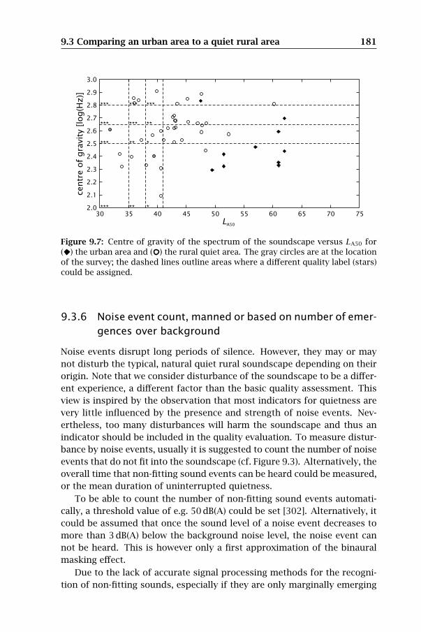
9.3 Comparing an urban area to a quiet rural area 181
3.0
2.9
2.8
2.7
2.6
2.5
2.4
2.3
2.2
2.1
2.075706560555045403530
centr
e o
f gra
vit
y [
log(H
z)]
LA50
Figure 9.7: Centre of gravity of the spectrum of the soundscape versus LA50 for( ) the urban area and ( ) the rural quiet area. The gray circles are at the locationof the survey; the dashed lines outline areas where a different quality label (stars)could be assigned.
9.3.6 Noise event count, manned or based on number of emer-
gences over background
Noise events disrupt long periods of silence. However, they may or may
not disturb the typical, natural quiet rural soundscape depending on their
origin. Note that we consider disturbance of the soundscape to be a differ-
ent experience, a different factor than the basic quality assessment. This
view is inspired by the observation that most indicators for quietness are
very little influenced by the presence and strength of noise events. Nev-
ertheless, too many disturbances will harm the soundscape and thus an
indicator should be included in the quality evaluation. To measure distur-
bance by noise events, usually it is suggested to count the number of noise
events that do not fit into the soundscape (cf. Figure 9.3). Alternatively, the
overall time that non-fitting sound events can be heard could be measured,
or the mean duration of uninterrupted quietness.
To be able to count the number of non-fitting sound events automati-
cally, a threshold value of e.g. 50 dB(A) could be set [302]. Alternatively, it
could be assumed that once the sound level of a noise event decreases to
more than 3 dB(A) below the background noise level, the noise event can
not be heard. This is however only a first approximation of the binaural
masking effect.
Due to the lack of accurate signal processing methods for the recogni-
tion of non-fitting sounds, especially if they are only marginally emerging
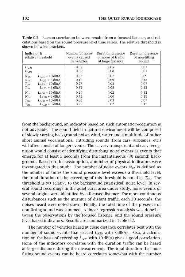
182 The Quiet Rural Soundscape
Table 9.2: Pearson correlation between results from a focused listener, and cal-culations based on the sound pressure level time series. The relative threshold isshown between brackets.
Indicator & Number of noise Duration presence Duration presencerelative threshold events caused of noise of traffic of non-fitting
by vehicles at large distance sound
LA50 0.36 0.05 0.01LA10 0.35 0.08 0.01
Ncn LA95 + 10 dB(A) 0.53 0.07 0.09Ncn LA95 + 3 dB(A) 0.10 0.09 0.32Tcn LA95 + 10 dB(A) 0.28 0.03 0.07Tcn LA95 + 3 dB(A) 0.32 0.08 0.12
Ncn LA50 + 10 dB(A) 0.20 0.02 0.12Ncn LA50 + 3 dB(A) 0.74 0.06 0.19Tcn LA50 + 10 dB(A) 0.05 0.03 0.07Tcn LA50 + 3 dB(A) 0.26 0.02 0.12
from the background, an indicator based on such automatic recognition is
not advisable. The sound field in natural environment will be composed
of slowly varying background noise: wind, water and a multitude of rather
short animal vocalisations. Intruding sounds (from cars, airplanes, etc.)
will often consist of longer events. Thus a very transparent and easy recog-
nition would consist of identifying disturbing noise events as events that
emerge for at least 3 seconds from the instantaneous (30 second) back-
ground. Based on this assumption, a number of physical indicators were
investigated in this study. The number of noise events Ncn is defined as
the number of times the sound pressure level exceeds a threshold level;
the total duration of the exceeding of this threshold is noted as Tcn. The
threshold is set relative to the background (statistical) noise level. In sev-
eral sound recordings in the quiet rural area under study, noise events of
several origins were identified by a focused listener. For more continuous
disturbances such as the murmur of distant traffic, each 30 seconds, the
noises heard were noted down. Finally, the total time of the presence of
non-fitting sound was summed. A linear regression analysis was done be-
tween the observations by the focused listener, and the sound pressure
level based indicators. Results are summarized in Table 9.2.
The number of vehicles heard at close distance correlates best with the
number of sound events that exceed LA50 with 3 dB(A). Also, a calcula-
tion on the basis of exceeding LA95 with 10 dB(A) gives a good correlation.
None of the indicators correlates with the duration traffic can be heard
at larger distance during the measurement. The total duration that non-
fitting sound events can be heard correlates somewhat with the number
9.4 Discussion — Multi-criteria assessment 183
of times LA95 is exceeded by at least 3 dB(A), but no simple linear relation
was found. From this analysis it can be concluded that the detection of the
disturbance of a soundscape by non fitting sounds can only be done by a
human observer or a more sophisticated source identification mechanism.
If the scope is narrowed however to sporadic road traffic noise at short dis-
tance, counting the number of times the instantaneous background level
measured as LA50 is exceeded during at least 3 seconds is the best alterna-
tive. Note that for noise mapping purposes, the problem of source iden-
tification is obsolete but knowing the overall (natural) background level is
not trivial.
9.4 Discussion — Multi-criteria assessment
Based on the views condensed from literature in soundscape research and
related fields, and based on the application in a case study, conclusions can
be drawn concerning the categorization and quality labeling of the quiet
rural soundscape. In this work a very particular context was considered
(Section 9.2.1); however, we have the impression that the proposed set
of indicators could also be used for assessing the quality of the acoustic
environment in urban parks and other quieter areas. Proposed limit values
will need to be adapted however.
The quiet rural soundscape finds its main societal value in its use for
quiet recreation, it may benefit the general mental health of the popula-
tion through its potential for psychological restoration, and it may help
to reduce mental fatigue. These functions require this environment to be
within reach of the city dweller. This leads us to propose a quality scale
rather than to impose strict limits. It allows conserving or creating some-
what lesser quality quiet rural soundscapes that are more within reach and
better ones that may be further away from densely populated living areas.
In particular, if this policy were adopted at a European level, it would allow
also to distinguish between member states with vast amounts of open area
and smaller overpopulated ones.
A first set of criteria are the perception based criteria. They have the
huge advantage that they sample the opinion of those visiting the area.
A possible disadvantage is their limited spatial resolution, which makes
them less useful for drawing detailed maps. The absence of calculation
models jeopardises their use in impact assessment and policy action plan-
ning. The first proposed indicator in this category is based on a sd ques-
tionnaire. A factor related to the pleasantness, naturalness or quietness of
the soundscape, derived by summing scores on sd’s given in Section 9.3.1,
184 The Quiet Rural Soundscape
should score at least positive for minimal quality. It could be quite useful
to add a second factor measuring the eventfulness or high fidelity of the
soundscape, but this could not be established in the case study. Within
the set of perception based criteria, it seems very useful to add a second
criterion based on perception of non-fitting sounds. The most versatile
way of including the degree-of-fit between sounds heard and the envi-
roscape/soundscape is to ask the users for it during the survey, at the same
time that they are asked about the sounds they heard and how loud they
were. The degree-of-fit question could then serve as a filter for the hear-
ing/loudness question. If both are assessed using an 11-point scale, the
simplest operation leading to such filtering would be to take the minimum
of the degree-of-non-fitting and the overall loudness. A conceptually easier
approach consists of the researcher deciding beforehand which sounds do
not fit the soundscape. Whatever the method used, the average over all
visitors of the overall loudness of any non-fitting sound should be below
1 if an 11-point answering scale is labeled 0 to 10 for minimal quality (sin-
gle ⋆). Even stricter requirements need to be imposed for higher quality
ranking.
A second class of indicators have a physical origin. These indicators
have the advantage of easy measurability and predictability. Thus they can
be used to clearly define the borders of the quiet rural area and to predict
the impact of policy action plans. Nevertheless these indicators go beyond
the classical LAeq and therefore require more extensive modeling. The case
study however clearly showed that this modeling is feasible. In order of
importance, we propose to include LA50 as a measure for the basic require-
ment that the background or ambient sound should have a low level; ml1
as an indicator for the dynamics of the soundscape linked to pleasing char-
acter and mental restorative potential; G for frequency content quantifying
low frequency mechanical noise; and Ncn, the number of clearly noticeable
non-fitting events, as a proxy for manned identification of sources. A first
proposal for limit values for different quality categorization is given in Ta-
ble 9.3. For several of the criteria there are little studies to back up a solid
proposal for these limits and more extensive research is required. These
cases are clearly indicated.
A final category of indicators is related to non-acoustical factors. They
are important to guarantee optimal use of the quiet rural soundscape.
Firstly, the region must be sufficiently large without any disrupting infras-
tructure dividing it. This criterion is related to the recreational use. The
proposed surface is based on a rough estimate of cycling/walking speed
and required duration of a visit needed to experience the beneficial effect
of the environment. The final criterion introduces biological, natural, and

9.4 Discussion — Multi-criteria assessment 185
Table 9.3: Proposed criteria for assessing the quality of the quiet rural soundscapeand proposed limit values. It is indicated (+) where more extensive research isrequired to refine the limits.
Indicator Quality indication Importance⋆ ⋆⋆ ⋆⋆⋆
sd — pleasantness to be investigated highnon-fitting sounds <1 <1+ <1+ mediumLA50 <41 dB(A) <38 dB(A) <35 dB(A) highml1 >0.5 >0.7 >0.9 mediumlog10(G) >2.5+ >2.65+ >2.8+ lowNcn (during 15 minutes) <20+ <10+ <5+ mediumcongruent area >10km2 >10km2+ >10km2+ lowbiolog./nature/landscape value low medium high medium
landscape value in the multi-criteria assessment. This is required, both be-
cause of well known inter-sensory effects and because a complete restora-
tive environment is aimed for.
The multi-criteria quality assessment methodology proposed above and
the selection of a complete set of indicators for this purpose is to our
knowledge the first of its kind. It is derived for a particular context but
could probably be extended to other context easily.


Part IVEffects of Noise at Home


Chapter10
Temporal Aspects and
Noise Annoyance
10.1 Classical approach to noise annoyance
In the first three parts of this work, the acoustic environment has been
studied from the viewpoint of soundscape research. The perception of
our sonic environment is considered to be inextricably bound up with and
influenced by all other environmental aspects, such as the landscape and
air quality, as well as by the state of mind of the observer. In this holistic
vision, the positive as well as the negative aspects of our sonic environment
are considered, which paves the road for acoustic design [141, 63].
It has been discussed in the introduction that this approach somewhat
conflicts with the current common practice to consider noise annoyance as
the major effect of noise pollution, and to use the energy equivalent sound
pressure level as its main indicator. Nevertheless, this classic approach
was found to be succesful for predicting effects of noise at the commu-
nity/residential scale. The most important sources of intruding noise at
home are related to traffic, industry or the neighbours [18]. Particularly
for road, railway and air traffic, the relation between community noise an-
noyance and energy equivalent sound pressure level (Lden in particular)
has been studied thoroughly [217]. The type of source plays an impor-
tant role; for example, railway noise is generally found to be less annoying
than road traffic noise, at equal exposure level. This is incorporated in the
legislation in several countries by the use of a railway bonus (see also the
next chapter). As already mentioned, physical noise characteristics other
than the average level, such as spectral or temporal effects, are usually ac-
counted for in legislation by the use of a penalty on the measured sound

190 Temporal Aspects and Noise Annoyance
pressure level (in particular for industrial noise, since spectral or temporal
characteristics may show a large situational variation in this case). Several
personal factors, such as age, gender, education level, noise sensitivity or
attitude towards the source, may also be modeled as a shift in effective
noise exposure [162, 218].
However, several shortcomings of this approach may be discerned [192,
193]. Firstly, in a typical sonic environment, various different sound
sources are present, but only single sources are assessed. It remains un-
solved how annoyance caused by single sources adds up to total annoy-
ance [19]. Secondly, due to the common separation of acoustic and non-
acoustic factors, interactions between the sonic environment, the observer
and its environment are neglected. Finally, the importance of the different
factors that modify noise annoyance is derived from aggregated data. It
remains unclear how these could be transferred to specific situations or
contexts.
10.2 Influence of temporal aspects
Research embracing the soundscape vision may lead to a better under-
standing of the processes that lead to noise annoyance [285, 192, 193, 175].
In Chapter 11, we will demonstrate how this can be done in a field experi-
ment. As we are particularly interested in the influence of temporal aspects
on noise annoyance, it is interesting to consider the extreme cases of high-
way traffic noise and railway noise: the former is continuous, the latter is
intermittent. By creating a realistic at-home context, in which people are
exposed to highway traffic and/or several train passages, simulating a real-
life schedule, the temporal aspect will be incorporated explicitly into the
design of the experiment. In an at-home context, people will most probably
not listen consciously to the soundscape all the time. As a consequence,
the holistic music-likeness indicator discussed in the previous parts may
be of less value in this case. However, temporal aspects may still influence
perceived annoyance in several ways.
On a longer time scale, the time intervals between train passages may
create a feeling of quietness (see Part III), as compared to highway traffic.
This is reflected in the high valued percentile sound pressure levels — LA50
and LA95 in particular — which are not influenced by the train passages.
Furthermore, in real life situations, people may get acquainted with the
fixed train shedule. This way, passages may be expected and anticipated,
which could lead to a feeling of control over the situation and to a reduced
annoyance.
10.2 Influence of temporal aspects 191
Temporal aspects on shorter time scales, related to the passage of a
single train, may also influence noise annoyance. One particular feature
of train noise is the rate at which the sound level increases when the train
approaches. This rate is influenced by the train speed and the distance
between the observer and the track. The rise time of a sound event has
been mentioned as a factor that increases annoyance caused by a sound
event. In the next chapter, we will show that for railway noise, differences
in rise time indeed explain a significant amount of annoyance variance not
accounted for by other factors. The startle effect could explain this in-
crease in annoyance, but this is unlikely for trains passing by at a distance
larger than a few tens of meters. A more plausible explanation could be
based on the hypothesis that noise has to be noticed, before it can become
annoying [103, 176, 281]. A short rise time could then trigger a notice
event [78].
Temporal aspects of noise may also cause the source to sound closer
by or further away, which in turn may have an additional influence on
noise annoyance. In Chapter 12, we will investigate how acoustic factors
influence auditory distance perception. In particular, we will show that the
rise time has a significant influence on perceived distance.


Chapter11
Experimental Investigation of
Noise Annoyance caused by
High-speed Trains
B. De Coensel, D. Botteldooren, B. Berglund,
Mats E. Nilsson, T. De Muer and P. Lercher
Submitted to Acta Acustica united with Acustica.
« « «
In this chapter, we will discuss a unique field experiment, which was
conducted to investigate the possible differences in perceived annoy-
ance of noise caused by the traffic on a highway, by conventional
trains and by high-speed trains, both conventional and magnetic levi-
tation. This research was financed by the Project Group Zuiderzeelijn,
The Netherlands. Results of this research were presented at the 12th
International Congress on Sound and Vibration [42].
11.1 Introduction
A difference in perceived annoyance between train and other traffic noise
at the same average sound level, has been observed in several field studies
in the past [105, 217]. In a number of countries, this observation has led
to a less restrictive regulation, or railway bonus, for train noise relative to
noise from other sources such as highways, major roads or aircraft. With
the introduction of high-speed trains and train-like transportation systems
based on magnetic levitation (maglev), the question has arisen whether a
difference in perceived annoyance of train and highway noise still exists.

194 Noise Annoyance caused by High-speed Trains
In particular, it is probable that spectral changes due to a higher fraction
of aerodynamic noise and shorter rise times due to high speeds, would
change the perceptions of high-speed train and maglev train noise.
Prior laboratory research by Fastl and Gottschling [99] showed no sig-
nificant difference in noise annoyance of a Transrapid 07 maglev train
at a speed of 400 km·h−1 and a conventional high-speed train at a speed
of 250 km·h−1, if presented at a comparable A-weighted equivalent sound
level. Conversely, Neugebauer and Ortscheid [234, 233] concluded that
maglev noise annoyance differed markedly from that of a conventional
train. An experiment by Vos [326, 327] showed that, if the outdoor ASEL’s
were set equal, the Transrapid 08 maglev train was more annoying than
a conventional intercity train, and approximately equally annoying as road
traffic.
In addition to the fact that these previous studies were inconclusive, a
few factors of potential importance were not explicitly considered in pre-
vious work. Firstly, in listening experiments with short fragments of noise,
listeners assess the perceived annoyance of noise. Such assessments cover
both perceived loudness and perceived character of noise (e.g., see [21]).
However, for short fragments of sound, the temporal effect may partly con-
tribute to the annoyance differences between trains and continuous traffic
sound. Longer exposures, containing several train passages as well as the
typical quiet periods in between, were necessary to include in this exper-
iment. Secondly, in real life, sounds may be annoying also because they
interfere with activities, like reading or relaxation. This aspect of noise
annoyance is not captured in traditional listening experiments, but is pos-
sible to assess, if the experiment is designed in the right way, as shown
in [153, 204]. Finally, it is well known from environmental noise ques-
tionnaire surveys that personal factors such as noise sensitivity influence
annoyance reports [162, 218]. Some of these factors have also been ob-
served in listening experiments [90, 323]. Therefore, the results may not
be valid and it may not be possible to generalize beyond the subgroup, if
this subgroup is not selected carefully to match the population concerning
these critical factors.
Recently, a small annoyance survey was conducted near the maglev line
in Shanghai [102]. Such annoyance surveys are not possible in Europe, be-
cause the magnetic levitation system has not yet been implemented but
for a test facility. Therefore a field experiment was specially designed
to solve as many of the above mentioned issues as possible. The exper-
iment differed significantly from the above cited earlier research. A real-
istic home-like setting was created, in which the panelists were asked to
relax while exposed to longer fragments of sound, including quiet peri-

11.2 The experiment 195
ods (Section 11.2.1). Traffic noise was reproduced in an ecologically valid
way, using multiple loudspeakers outdoors to simulate pass-by sound (Sec-
tion 11.2.2). The set of panelists was selected to be representative of the
Dutch population in factors known to be important modifiers of noise an-
noyance (Section 11.2.3). For the outline of the listening test, menus of train
passages delimiting longer exposure durations were used (Section 11.2.4).
The method of master scaling by which perceived annoyance was scaled,
calibrated the scales used by different participants to a common master
scale (Section 11.2.5).
The main goal of this research was to investigate the possible differ-
ences in annoyance, on the one hand, between magnetic levitation and
conventional high speed trains and, on the other hand, between highway
noise and train noise. Next to this, the influence of some additional factors
on noise annoyance were studied, such as the distance between the source
and the listener, the speed of the source and the rise time of the sound.
11.2 The experiment
11.2.1 Sound reproduction in a realistic setting
As a natural setting, a holiday cottage in Westkapelle (Zeeland, The Nether-
lands) was selected because of its quiet environment and accessibility.
During the experiment, subgroups of participants were seated in the liv-
ing room, reading a magazine, engaging in light conversation or having
something to drink. Figure 11.1 shows the cottage and its environment.
Much attention was paid to creating a realistic reproduction of the three-
dimensional indoor sound field, produced by a moving train outside the
house. Observe that the goal was to obtain an “ecologically valid” [128]
reproduction rather than physical precision. It is difficult to produce the
effect of a house by signal processing and playback through headphones
or indoor loudspeakers, and to accomplish a natural feeling of the sound
field. Therefore, it was decided to reproduce the sound field, as recorded
outdoors, outside the experimental cottage. This approach has already
been demonstrated to be valid [204].
It was assumed that two-channel recording would be accurate enough
to get a good three-dimensional representation indoors. This hypothesis
was checked for low speed trains at short distance. The indoor sound field,
in another house close to an existing railway and produced by a real train,
was compared to that reproduced artificially using two loudspeakers. The
procedure consisted of 2 phases. First, during the passage of a train, the
sound was recorded outdoor by 2 microphones separated 20 m from each
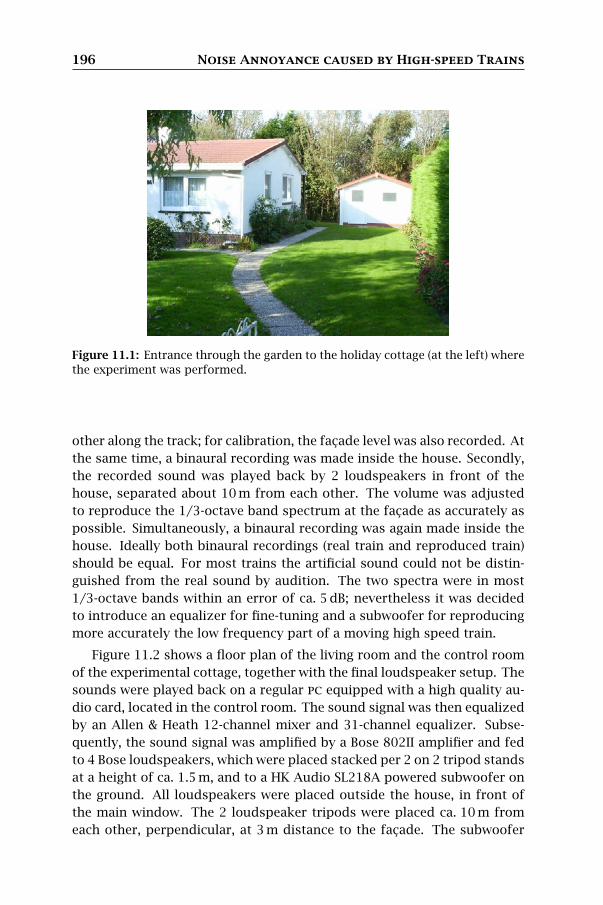
196 Noise Annoyance caused by High-speed Trains
Figure 11.1: Entrance through the garden to the holiday cottage (at the left) wherethe experiment was performed.
other along the track; for calibration, the façade level was also recorded. At
the same time, a binaural recording was made inside the house. Secondly,
the recorded sound was played back by 2 loudspeakers in front of the
house, separated about 10 m from each other. The volume was adjusted
to reproduce the 1/3-octave band spectrum at the façade as accurately as
possible. Simultaneously, a binaural recording was again made inside the
house. Ideally both binaural recordings (real train and reproduced train)
should be equal. For most trains the artificial sound could not be distin-
guished from the real sound by audition. The two spectra were in most
1/3-octave bands within an error of ca. 5 dB; nevertheless it was decided
to introduce an equalizer for fine-tuning and a subwoofer for reproducing
more accurately the low frequency part of a moving high speed train.
Figure 11.2 shows a floor plan of the living room and the control room
of the experimental cottage, together with the final loudspeaker setup. The
sounds were played back on a regular pc equipped with a high quality au-
dio card, located in the control room. The sound signal was then equalized
by an Allen & Heath 12-channel mixer and 31-channel equalizer. Subse-
quently, the sound signal was amplified by a Bose 802II amplifier and fed
to 4 Bose loudspeakers, which were placed stacked per 2 on 2 tripod stands
at a height of ca. 1.5 m, and to a HK Audio SL218A powered subwoofer on
the ground. All loudspeakers were placed outside the house, in front of
the main window. The 2 loudspeaker tripods were placed ca. 10 m from
each other, perpendicular, at 3 m distance to the façade. The subwoofer

11.2 The experiment 197
control room
openedwindow
H
6
7
3 4 5
2
1
L
façade level
subwoofer
Figure 11.2: Schematic drawing of the experimental cottage (not to scale). The dif-ferent seats of the panelists are shown (1–7), as well as the seat of the experimentalleader (L) and of the artificial head (H) for binaural recordings.
was placed in front of the window in between both tripods, at about 50 cm
from the façade. This loudspeaker setup was located in front of a slightly
opened window of the experimental cottage, invisible to the panelists en-
tering the house.
The façade level was measured continuously during all experimental
sessions, using a B&K Investigator 2260 sound level meter with a B&K 4189
free field microphone (5 cm from the window at 75 cm height). The sound
level meter was also used to calibrate the playback system. For this cali-
bration, pink noise was played back and adjusted to give a façade level of
91 dB with a flat 1/3-octave band spectrum. The equalizer accomplished a
flat (± 3 dB for all 1/3-octave bands) spectrum between 30 Hz and 16 kHz.
The façade attenuation and the reverberation in the experimental room,
both modify the spectrum and temporal characteristics of the sound. The
indoor sound field was monitored by an artificial head placed among the
panelists. The sound pressure level difference between the façade and at
the ear of this artificial head was approximately 21 dB. Since it would not
be possible to see a train passage from the window because of plenty of
trees, no visual presentation of passing trains was considered appropriate.

198 Noise Annoyance caused by High-speed Trains
11.2.2 Sample collection and preparation
Two-channel recordings were conducted for three types of trains. Two mi-
crophones were placed at 20 m distance from each other along the track,
1.5 m above ground level. tgv trains at high speed were recorded in Be-
loeil (Belgium), a site near the tgv connection between Brussels and Lille
(France). Dutch intercity (ic) trains of the new type (duplex) were recorded
in Oudenbosch near Roosendaal (The Netherlands); at this same site the
tgv traveling at low speed from Brussels to Rotterdam was also recorded.
At the maglev test track in Lathen (Germany), the Transrapid 08 train was
recorded at speeds of approx. 200 km·h−1, 300 km·h−1 and 400 km·h−1. As
master scaling references, the sound of the E40 highway was also recorded
near Ghent (Belgium). To be able to assess the influence on annoyance of
the distance to the track, 4 recording distances were included (25 m, 50 m,
100 m, and 200 m). All recordings were made in free field without noise
barriers. Not only the spectrum and temporal change were reproduced ex-
actly, but also the sound level, as if the house would have been located at
the measurement site.
From the many train recordings made at each site, the passage of high-
est quality was selected in each category of recording, and for these, 45-
second single passage fragments were cut. It was important to expose
the panelists to sufficient and natural durations of noise. Therefore, they
had to be exposed to “experimental sound” during at least 10 minutes
(henceforth called a menu). To create a realistic exposure situation within
a 10-minute menu, it should be composed of the same train type, at the
same distance and speed. Menus with 2 or 4 passages were created because
4 passages in 10 minutes already represents the natural time-schedule max-
imum, and 2 passages in 10 minutes represents a minimum passage rate
with inter-passage background sound. Less than two passages are not use-
ful because the inter-event silence is non-defined in this case. Apart from
the 45-second fragments recorded at the four distances to the track, a 10-
minute highway sound was recorded at 50 m distance to the closest lane.
Table 11.1 summarizes the sound exposure (ASEL) and sound levels
(LAeq,45s) associated with the 45-second passages used in the 10-minute
menus. It should be mentioned that the level of the ic train at 25 m happens
to be lower than the level at 50 m. This inconsistency is due to the fact
that the selected high-quality sound fragments do not necessarily originate
from identical train passages. There is always a natural spread in the speed
and the number of wagons of the different passages of the same type of
train. As an illustration, Figures 11.3 and 11.4 show the A-weighted sound
exposure level in 1/3-octave bands for some of the experimental traffic
sounds, as recorded in free field.
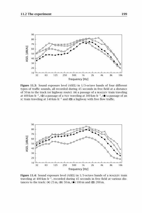
11.2 The experiment 199
10
20
30
40
50
60
70
80
90
32 63 125 250 500 1k 2k 4k 8k 16k
frequency [Hz]
ASEL [
dB(A
)]
Figure 11.3: Sound exposure level (ASEL) in 1/3-octave bands of four differenttypes of traffic sounds, all recorded during 45 seconds in free field at a distanceof 50 m to the track (or highway route): ( ) a passage of a maglev train travelingat 400 km·h−1, ( ) a passage of a tgv traveling at 300 km·h−1, ( ) a passage of anic train traveling at 140 km·h−1 and ( ) a highway with free flow traffic.
10
20
30
40
50
60
70
80
90
32 63 125 250 500 1k 2k 4k 8k 16k
frequency [Hz]
ASEL [
dB(A
)]
Figure 11.4: Sound exposure level (ASEL) in 1/3-octave bands of a maglev traintraveling at 400 km·h−1, recorded during 45 seconds in free field at various dis-tances to the track: ( ) 25 m, ( ) 50 m, ( ) 100 m and ( ) 200 m.

200 Noise Annoyance caused by High-speed Trains
Table 11.1: Traffic sounds used in the 10-minute menus of the experiment. Soundexposure levels (ASEL) for one 45-second train passage and sound level (LAeq,45s) ofhighway traffic, at 25–200 m distance to track or route, all free field recordings. Toobtain the corresponding LAeq,45s (or ASEL levels), subtract (or add) 10 log(45) =16.5 dB(A). To obtain the LAeq,10min values for the corresponding 2-train or 4-trainmenus, subtract 8.2 dB(A) or 5.2 dB(A), respectively, from the corresponding 1-trainLAeq,45s values; to obtain the ASEL values add 3 dB(A) or 6 dB(A), respectively. TheLAeq,10min value of the 10-minute highway menu is about the same as the LAeq,45s
value of the highway at 50 m.
Sound source Distance to track25 m 50 m 100 m 200 m
Outdoor ASEL [dB(A)]
maglev 200 km·h−1 80.1 72.9 71.3 59.7300 km·h−1 86.3 83.0 80.3 69.6400 km·h−1 92.6 88.7 85.2 70.4
tgv 140 km·h−1 84.1 78.3 73.6 64.4300 km·h−1 92.8 90.6 86.9 83.0
ic 140 km·h−1 75.0 80.9 72.4 62.0
Outdoor LAeq,45s [dB(A)]
Highway free flow 71.6 66.1 62.6 55.3
For master scaling, 7 traffic-noise-like reference sound fragments of
45 seconds duration were included in the experiment. These extra refer-
ence sounds with varying level were sound edited by changing amplitude
and spectrum of the highway noise recorded at 50 m distance to the high-
way.
11.2.3 Selection of a representative panel
In contrast to previous experimental work on noise annoyance caused by
high speed trains, in which small “convenient” samples of test persons were
recruited, the selection of panelists was here made to guarantee a repre-
sentative sample of panelists. A questionnaire was administered at the
doorstep of the homes of approximately 1500 persons, all living within a
distance of 15 km from the experimental site. In an introductory letter, one
inhabitant of the house was invited to participate in the study. The prereq-
uisites were that (s)he had to fill in and send the questionnaire back to the
address on the enclosed stamped envelope. A compensation of 100 euro
was offered for participation.
The questionnaire contained selected questions that had been asked to
a representative sample of the target population in a recent survey. The

11.2 The experiment 201
Table 11.2: Comparison between the panelists and the reference population onvarious criteria. Mean and standard deviation is shown; the results for the secondseries of criteria are on an 11-point scale and vary from 0 (“not at all”/“bad”) to10 (“very”/“good”).
Criterium Participants Reference
Gender [% male / % female] 51 / 49 48 / 52Age [year] 45.1± 13.4 45.6± 17.7
Noise sensitivity 5.1± 2.4 4.6± 2.6Quality of traffic noise in the living environment 6.6± 2.4 6.4± 2.3Quality of the living environment 7.6± 1.4 7.3± 1.3Feeling afraid or frightened 2.4± 2.0 2.3± 2.1
structure of the Dutch population was inferred to be representative from a
recent rivm survey [112] and partly from a Eurobarometer questionnaire.
Our questionnaire contained (standard) questions on environmental noise
as regards perception, annoyance and sleep disturbance. Included were
evaluations of the quality of the neigbourhood in terms of housing and
environmental pollution of other types than noise, as well as evaluations
of overall satisfaction with the current living situation. Other questions
addressed basic demographic variables such as age, gender, education,
housing, family size and work arrangements. A set of questions were also
included on general and mental health, hearing ability, environmental back-
ground, opinion and worry, and environmental sensitivity.
A procedure to draw panelists, representative of the target population,
from the 255 replies received involved three stages. Stage 1 removed po-
tential panelists on the basis of their age and hearing ability (information
had already been given in the introductory letter). Stage 2 further removed
those that were very dissimilar from the typical Dutch person on the basis
of binary coding of most of the other criteria included in the question-
naire. This stage implicitly assessed individual responses on the questions
as regards their concordance with the response profile of the typical Dutch
person in the reference survey. Stage 3 finally selected panelists on the ba-
sis of fuzzy resemblance to the typical Dutch person on the most critical
criteria of annoyance surveys, such as age, gender, education, noise sensi-
tivity, feeling afraid or frightened, hearing train noise at home, quality of
traffic noise in the living environment, quality of the living environment,
general health, and illness. Finally, ca. 100 representative participants were
selected. Table 11.2 shows a comparison of the panelists with the Dutch
target population as regards the mean and standard deviation of some of
the selection criteria used and mentioned above.
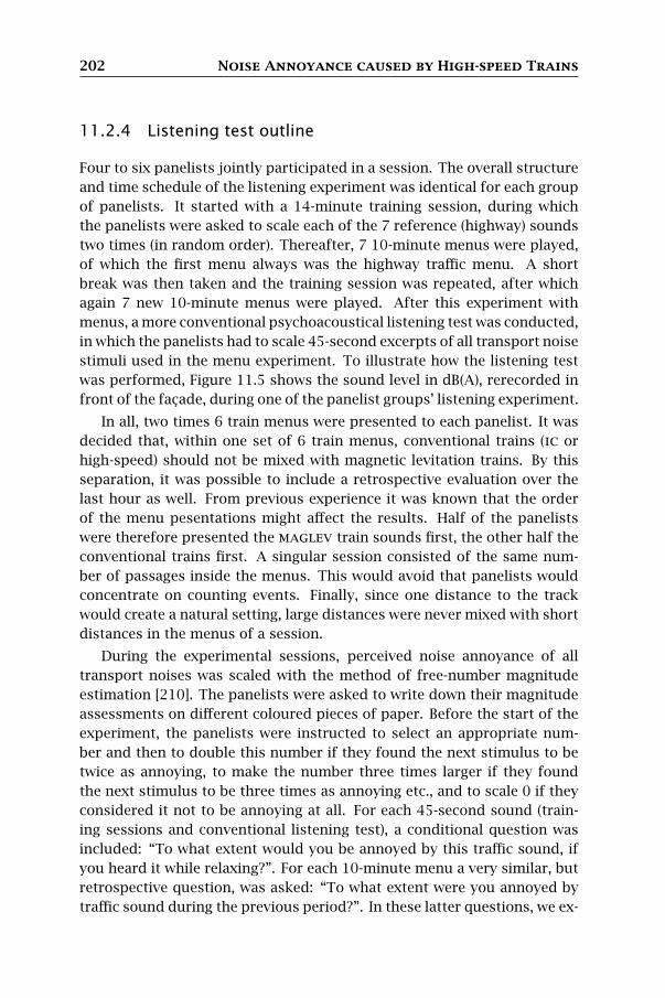
202 Noise Annoyance caused by High-speed Trains
11.2.4 Listening test outline
Four to six panelists jointly participated in a session. The overall structure
and time schedule of the listening experiment was identical for each group
of panelists. It started with a 14-minute training session, during which
the panelists were asked to scale each of the 7 reference (highway) sounds
two times (in random order). Thereafter, 7 10-minute menus were played,
of which the first menu always was the highway traffic menu. A short
break was then taken and the training session was repeated, after which
again 7 new 10-minute menus were played. After this experiment with
menus, a more conventional psychoacoustical listening test was conducted,
in which the panelists had to scale 45-second excerpts of all transport noise
stimuli used in the menu experiment. To illustrate how the listening test
was performed, Figure 11.5 shows the sound level in dB(A), rerecorded in
front of the façade, during one of the panelist groups’ listening experiment.
In all, two times 6 train menus were presented to each panelist. It was
decided that, within one set of 6 train menus, conventional trains (ic or
high-speed) should not be mixed with magnetic levitation trains. By this
separation, it was possible to include a retrospective evaluation over the
last hour as well. From previous experience it was known that the order
of the menu pesentations might affect the results. Half of the panelists
were therefore presented the maglev train sounds first, the other half the
conventional trains first. A singular session consisted of the same num-
ber of passages inside the menus. This would avoid that panelists would
concentrate on counting events. Finally, since one distance to the track
would create a natural setting, large distances were never mixed with short
distances in the menus of a session.
During the experimental sessions, perceived noise annoyance of all
transport noises was scaled with the method of free-number magnitude
estimation [210]. The panelists were asked to write down their magnitude
assessments on different coloured pieces of paper. Before the start of the
experiment, the panelists were instructed to select an appropriate num-
ber and then to double this number if they found the next stimulus to be
twice as annoying, to make the number three times larger if they found
the next stimulus to be three times as annoying etc., and to scale 0 if they
considered it not to be annoying at all. For each 45-second sound (train-
ing sessions and conventional listening test), a conditional question was
included: “To what extent would you be annoyed by this traffic sound, if
you heard it while relaxing?”. For each 10-minute menu a very similar, but
retrospective question, was asked: “To what extent were you annoyed by
traffic sound during the previous period?”. In these latter questions, we ex-

11.2 The experiment 203
trainingsession
1 highway traffic menu6 train menus
trainingsession
1 highway traffic menu6 train menus
conventionallistening test
30
40
50
60
70
80
90
100
8:30 9:00 9:30 10:00 10:30 11:00 11:30 12:00 12:30
LA
eq,1
s[d
B(A
)]
time
Figure 11.5: Sound pressure level rerecorded in front of the façade during onepanelist groups’ participation in the whole listening test: two training sessions, twomenu sessions and one conventional psychoacoustical experiment with references.
plicitly did not want to refer to train noise, since we wanted the panelists
to decide themselves whether the sound period they last heard sounded
like train-contaminated or not.
11.2.5 Master scaling
In all experimental sessions, the 7 road-traffic-noise-like reference sounds
helped the panelists to define their own scaling context. The annoyance
values given to these reference sounds made it possible to control for the
individual panelists’ choice-of-number behaviour in scaling the target train
sounds. It would also control the influence of personal factors such as
noise sensitivity. To get rid of these effects, each individual panelist’s an-
noyance scale was calibrated by the aid of the reference to the common
master scale [13].
A graphical illustration of the master scale transformation applied to
the annoyance reference data of one of the panelists is given in Figure 11.6.
The average annoyance reported for each of the 7 reference sound levels of
road traffic noise is plotted in lin-log coordinates against their sound levels,
LAeq,45s, measured at the façade. Individual psychophysical functions are
fitted to the reference data (open circles). They are of the form
Ar = a+ b log Sr (11.1)
where Ar is the reported annoyance during the training session, and log Sris the corresponding “road traffic noise” reference (r ) sound level in dB(A).
The constants a and b will be different for each panelist and will depend
on their choice-of-number behaviour in the particular scaling context. The

204 Noise Annoyance caused by High-speed Trains
empirically derived master functions for the group of 100 panelists (dashed
line in Figure 11.6) were then used to transform the free number magnitude
estimations of the train or road traffic menus for each individual, Ae, to the
corresponding annoyance values R in master scale units:
R = −62.9+ 1.45Ae − a
b(11.2)
The slope of the master function was set to 1.45, which is the average slope
of all the individual psychophysical functions, whereas the intercept was
set to produce a value of “zero” for the most quiet train menu. The reason
for the latter choice was that a majority of the panelists (84 %) reported
their annoyance to be zero for this menu, and a majority of the panelists
reported annoyance to be greater than zero for all other menus.
The choice of a logarithmic psychophysical function (Eq. 11.1) was a
compromise. In previous magnitude estimation experiments of loudness
[13, 21], a power function of the form logA = c + d log S was found to
fit the empirical data best. However, in this experiment noise annoyance,
rather than loudness, was scaled and thus, obviously, also a value of zero
(= not at all annoyed) had to be handled, although the noise was heard and
its loudness was above zero. The power function (after removal of zeros)
did not fit the data better than the chosen logarithmic function.
11.2.6 Data quality analysis
The master scaling made it possible to investigate the quality of the ex-
perimental data in two ways, as panelists’ test-retest reliability and as their
scaling ability. The 7 reference sounds were presented 6 times to each pan-
elist; twice in the two training sessions and twice in the last conventional
listening test. The set of 6 reference scale values were used to determine
each panelist’s test-retest reliability of annoyance. Table 11.3 shows the
Pearson’s coefficient of correlation for these 6 annoyance scales, averaged
over all panelists. The test-retest reliability was very good, between 0.81
and 0.88, and the standard error was low, between 0.014 and 0.019.
The deviation from the proposed master function (Eq. 11.1) was used
to assess the data quality and annoyance scaling ability for each panelist
and to trace errors and inaccuracies. Table 11.4 shows the distribution of
constants of the panelists’ individual psychophysical functions (Eq. 11.1).
The average annoyance variance explained by sound level (LAeq,45s) of the
reference road traffic sounds was found to range from 88 % to 95 %. All
panelists were able to produce acceptable individual logarithmic functions
of annoyance as a function of sound level to the reference. They have

11.2 The experiment 205
0
10
20
30
40
50
60
70
80
40 50 60 70 80 90
R = 55, master–scaled annoyance
A = 70, assessment
annoyance
road traffic reference sound level [dB(A)]
Figure 11.6: Calculation of master-scaled annoyance, using one panelists’ empir-ical psychophysical function of the reference sounds (data points with solid line)and the master function for the same sounds (dashed line; obtained as averagefunction for all panelists).
Table 11.3: Test-retest reliability of panelists’ perceived noise annoyance of the7 reference road traffic sounds. Each cell contains an arithmetic mean of Pearson’scoefficient (r ) and its standard error.
Training session 1 Training session 2 Conventional testSet 1 Set 2 Set 1 Set 2 Set 1 Set 2
Training Set 1session 1
Set 2 0.82±0.015
Training Set 1 0.86 0.87session 2 ±0.014 ±0.016
Set 2 0.86 0.88 0.87±0.017 ±0.020 ±0.019
Conventional Set 1 0.83 0.83 0.82 0.85test ±0.015 ±0.021 ±0.019 ±0.020
Set 2 0.84 0.85 0.81 0.84 0.82±0.015 ±0.019 ±0.016 ±0.019 ±0.015

206 Noise Annoyance caused by High-speed Trains
Table 11.4: Distribution of constants of the panelists’ individual psychophysicalfunctions (Eq. 11.1). The number of data sets refers to the average of 4 or 2 rawannoyance values, which was taken for each of the 7 reference sounds to calculatethe psychophysical functions.
Data Psychophysical functionSets r 2 a b
Training session 1 & 2 4 0.947 −67.27 1.449±0.077 ±61.28 ±1.230
Conventional test 2 0.881 −47.57 1.105±0.118 ±48.17 ±0.948
thus produced acceptable annoyance data in order to transform these to
a common master scale of annoyance; no panelists were excluded from
further data analysis.
11.3 Results
The main listening experiment with menus was unique in a number of
aspects. One important novelty compared to previous laboratory experi-
ments is that participants were asked to judge annoyance over a longer pe-
riod of time — Fastl and Gottschling’s experiment [99] forms an exception.
During the 10-minute periods, the panelists were engaged in low attention,
relaxing activities such as reading a magazine, making a conversation or
having something to drink. In order to find out how this new approach af-
fected the results, a subsequent experiment was included, which was more
comparable to earlier experiments on train noise (e.g. [327]).
11.3.1 Main field experiment with 10-minute menus
The panelists’ master scale values of annoyance were averaged for each
menu in the field experiment. A stepwise multiple linear regression anal-
ysis was performed, with average master scaled annoyance as dependent
variable and (a) time averaged A-weighted façade exposure LAeq,10min, (b)
distance to the source (logarithmic) and (c) source type, as independent
variables. Table 11.5 summarizes the results. In the first model, sound
level was the only independent variable; this model explained 80 % of the
variance in annoyance. In the second model, distance to track was added to
sound level as an independent variable; this model increased the variance
explained to 85 % (F-change = 14.49, df1 = 1, df2 = 46, p < 0.001). Thus,
distance to source explained a significant additional part of the annoyance

11.3 Results 207
Table 11.5: Stepwise multiple regression analysis of acoustic variables on per-ceived annoyance of train and highway traffic sounds, for the main field experi-ment with 10-minute menus. The Pearson’s correlation coefficients of the variablesentered in the regression analysis are shown at the bottom.
Model Model fit F-change Independent Coefficient t-valuefit (r2) increase Variables
(r2-change)
1. 0.80 0.80 187.48∗∗∗ LAeq,10min 1.18 13.69∗∗∗
2. 0.85 0.05 14.49∗∗∗ LAeq,10min 0.92 9.17∗∗∗
log10(distance) −10.74 −3.81∗∗∗
3. 0.85 0.00 0.13 LAeq,10min 0.96 8.22∗∗∗
log10(distance) −10.17 −3.33∗∗
maglev [0,1] 1.45 0.27tgv [0,1] 0.85 0.16ic [0,1] 2.27 0.40
∗p < 0.05, ∗∗p < 0.01, ∗∗∗p < 0.001.
Label Variable ann leq dist mag tgv
ann Annoyanceleq LAeq,10min 0.894dist log10(distance) −0.754 −0.659mag maglev [0,1] −0.023 −0.038 0.009tgv tgv [0,1] 0.132 0.224 0.006 −0.682ic ic [0,1] −0.179 −0.290 0.004 −0.433 −0.308
variance not accounted for by sound level. In the third model, source-type
was included as a third independent variable along with sound level and
distance. Source type was defined on a nominal scale: maglev, tgv, ic
and highway. It was introduced in the analysis as three dummy variables,
coded 0 and 1 (the highway noise source type corresponds to the case that
these variables are all zero). The inclusion of source type did not increase
significantly (F-change < 1.0) the proportion of variance explained. This
suggests that statistically, there is no additional contribution of source type
on perceived annoyance over and above the effects of sound level and dis-
tance. It can therefore be concluded that magnetic-levitation based trans-
portation systems are not significantly more annoying than conventional
rail based systems (same façade LAeq and same distance are prerequisites).
Moreover, railway noise was not found to be systematically less annoying
than highway traffic noise. This means that no support for a railway bonus
was found in this experiment; at least it was not as obvious that it could
be observed using linear statistics.
Figure 11.7 gives an overview of the annoyance functions for the 10-
minute menus as a function of LAeq. The dashed line indicates the master
function of annoyance for the road-traffic-like sounds used as references.

208 Noise Annoyance caused by High-speed Trains
–10
0
10
20
30
40
50
60
70
30 40 50 60 70 80
annoyance [
maste
r scale
unit
s]
LAeq,10min [dB(A)]
(b)
–10
0
10
20
30
40
50
60
70
30 40 50 60 70 80
annoyance [
maste
r scale
unit
s]
LAeq,10min [dB(A)]
(a)
Figure 11.7: Average master scaled annoyance of the menus versus LAeq,10min (a)for 2 events per 10-minute menu and (b) for 4 events per 10-minute menu, fordifferent types of train sounds: ( ) ic train, ( ) tgv and ( ) maglev train. Incomparison, the annoyance for the highway traffic ( ) is also shown. Standarderror on means is indicated, as well as the master function (dashed line).

11.3 Results 209
–10
0
10
20
30
40
50
60
70
30 40 50 60 70 80
annoyance [
maste
r scale
unit
s]
LAeq,10min [dB(A)]
(b)
–10
0
10
20
30
40
50
60
70
30 40 50 60 70 80
annoyance [
maste
r scale
unit
s]
LAeq,10min [dB(A)]
(a)
Figure 11.8: Average master scaled annoyance of the menus versus LAeq,10min
showing (a) the noise event rise speed and (b) the distance to the track as thesize of the circles. The master function is also indicated (dashed line).

210 Noise Annoyance caused by High-speed Trains
The shorter rise time of the noise of arriving high speed trains may cre-
ate more annoyance than a conventional train can do. Figure 11.8(a) shows
the rise speeds in dB(A)·s−1 in proportion to circle sizes. These values
were calculated for all sound events included in this experiment by fitting
a straight line through the initial increase in sound level. The accelerat-
ing growth of annoyance with increasing LAeq may be explained by the rise
time. In Figure 11.8(b) the size of the circles is instead proportional to the
distance to the track. For LAeq in the interval between 50 and 65 dB(A), an-
noyance is clearly lower for train passages at larger distances than for train
passages at closer distances or road traffic noise (dashed line). This could
indicate that a possible noise annoyance bonus for train noise would only
hold at larger distances from the track, and only in the latter LAeq interval.
In order to explore the effects of train speed and rise time on perceived
annoyance, a stepwise multiple linear regression analysis was conducted,
excluding the highway noise menus. Table 11.6 summarizes the results.
In the first model, sound level LAeq,10min was included as the only indepen-
dent variable; this model explained 80 % of the variance in annoyance (cf.
Model 1 in Table 11.5). In the second model, train speed (km·h−1), distance
to the track (logarithmic) and rise speed (dB(A)·s−1) were added to sound
level as independent variables; this increased the explained variance to 88 %
(F-change = 9.34, df1 = 3, df2 = 43, p < 0.001). Apart from sound level, dis-
tance and rise speed significantly contributed to the variance explained. In
the third model, train type was added as an independent variable, which
was defined on a nominal scale (maglev, tgv, and ic), and included in the
analysis using two dummy variables coded 0 and 1. The inclusion of train
type again did not increase the proportion explained variance significantly
(F-change = 1.20), suggesting that train type did not explain perceived an-
noyance over and above the effects of sound level, distance and rise speed.
11.3.2 Conventional listening test
In the conventional listening experiment, the sounds were presented as
short 45-second fragments containing the sound of one train passage and
highway excerpts. Figure 11.9 shows the results of these master scaled an-
noyance values as a function of time averaged A-weighted façade exposure,
LAeq,45s. A railway penalty can be observed, both in regard to the artificial
reference sounds as well as to the highway sounds. Figure 11.10 shows the
annoyance as a function of rise speed (a) and distance to the track (b).
A stepwise multiple linear regression analysis was performed, with av-
erage master scaled annoyance as dependent variable and (a) LAeq,45s, (b)
distance to the source and (c) source type, as independent variables (Ta-

11.3 Results 211
Table 11.6: Stepwise multiple regression analysis of acoustic variables on per-ceived annoyance of train sounds (no highway traffic sounds), for the main fieldexperiment with 10-minute menus. The Pearson’s correlation coefficients of thevariables entered in the regression analysis are shown at the bottom.
Model Model fit F-change Independent Coefficient t-valuefit (r2) increase Variables
(r2-change)
1. 0.80 0.80 181.25∗∗∗ LAeq,10min 1.18 13.46∗∗∗
2. 0.88 0.08 9.34∗∗∗ LAeq,10min 0.59 4.02∗∗∗
Speed 0.00 −0.36log10(distance) −11.71 −3.70∗∗∗
Rise speed 0.71 2.97∗∗
3. 0.88 0.00 1.20 LAeq,10min 0.48 2.41∗
Speed 0.01 0.72log10(distance) −14.18 −3.35∗∗
Rise speed 0.67 2.72∗∗
maglev [0,1] −4.02 −1.55tgv [0,1] −1.76 −0.80
∗p < 0.05, ∗∗p < 0.01, ∗∗∗p < 0.001.
Label Variable ann leq spd dist rise mag
ann Annoyanceleq LAeq,10min 0.893spd Speed 0.431 0.534dist log10(distance) −0.753 −0.658 −0.001rise Rise speed 0.790 0.793 0.708 −0.437mag maglev [0,1] −0.007 −0.017 0.552 0.000 0.188tgv tgv [0,1] 0.145 0.243 −0.190 0.000 0.100 −0.707
ble 11.7). The first model with sound level as the only independent variable,
explained 92 % of the variance in annoyance. In the second model, distance
was added as an independent variable, but this did not increase the variance
explained (F-change < 1.0). In the third model, source type was included as
an independent variable along with sound level and distance. The inclusion
of source type significantly increased the proportion of variance explained
(F-change = 8.50, df1 = 3, df2 = 22, p < 0.001), suggesting that source type
influences perceived annoyance over and above the effect of sound level
and distance. The main cause of this latter effect was the lower annoyance
of road-traffic noise as compared to train noise (see Figure 11.9). A fourth
model was constructed, with sound level and source type as independent
variables. Using the regression coefficients and Equation 11.2, these data
supports a railway malus between 3.5 dB(A) and 6.5 dB(A).
A stepwise multiple linear regression analysis was also performed sep-
arately for the train noises (Table 11.8). The first model, in which sound

212 Noise Annoyance caused by High-speed Trains
–10
0
10
20
30
40
50
60
70
30 40 50 60 70 80
annoyance [
maste
r scale
unit
s]
LAeq,45sec [dB(A)]
Figure 11.9: Average master scaled annoyance versus LAeq,45s for the conventionallistening test, for different types of train sounds: ( ) ic train, ( ) tgv, ( ) maglev
train. In comparison, the annoyance for the highway traffic ( ) is also shown.Standard error on means is indicated, as well as the master function (dashed line).
level LAeq,45s was included as the only independent variable, explained 95 %
of the variance in annoyance. In the second model, train speed, distance
to the track and rise speed were added to sound level as independent vari-
ables. This increased the variance explained to 98 % (F-change = 12.50,
df1 = 3, df2 = 19, p < 0.001). Apart from sound level, also rise speed con-
tributed significantly to the variance explained. The third model, in which
train type was added as an independent dummy variable, did not signifi-
cantly increase the proportion explained variance (F-change < 1.0). These
results suggest that, in this conventional listening test, there is no differ-
ence in perceived annoyance between different types of trains, over and
above the effect of sound level and rise speed.
One has to note that the number of responses to each stimulus was
smaller in the main experiment (10-minute menus) than in the conventional
listenig test (45-second passages). This explains why the standard errors
are lower and the explained variance is higher in the latter experiment.
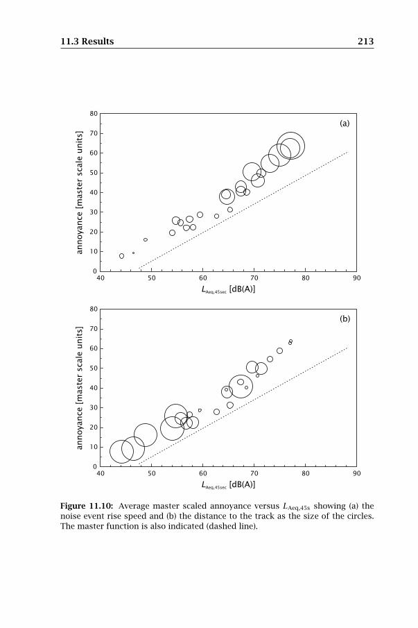
11.3 Results 213
0
10
20
30
40
50
60
70
80
40 50 60 70 80 90
annoyance [
maste
r scale
unit
s]
LAeq,45sec [dB(A)]
(b)
0
10
20
30
40
50
60
70
80
40 50 60 70 80 90
annoyance [
maste
r scale
unit
s]
LAeq,45sec [dB(A)]
(a)
Figure 11.10: Average master scaled annoyance versus LAeq,45s showing (a) thenoise event rise speed and (b) the distance to the track as the size of the circles.The master function is also indicated (dashed line).

214 Noise Annoyance caused by High-speed Trains
Table 11.7: Stepwise multiple regression analysis of acoustic variables on per-ceived annoyance of train and highway traffic sounds, for the conventional listen-ing test (45-second passages). The Pearson’s correlation coefficients of the vari-ables entered in the regression analysis are shown at the bottom.
Model Model fit F-change Independent Coefficient t-valuefit (r2) increase Variables
(r2-change)
1. 0.92 0.92 289.91∗∗∗ LAeq,45s 1.63 17.03∗∗∗
2. 0.92 0.00 0.57 LAeq,45s 1.70 12.74∗∗∗
log10(distance) 2.64 0.75
3. 0.96 0.04 8.50∗∗∗ LAeq,45s 1.72 15.83∗∗∗
log10(distance) 3.01 1.12maglev [0,1] 9.43 4.95∗∗∗
tgv [0,1] 7.16 3.56∗∗
ic [0,1] 5.70 2.31∗
4. 0.96 − − LAeq,45s 1.63 21.88∗∗∗
maglev [0,1] 9.24 4.85∗∗∗
tgv [0,1] 7.27 3.60∗∗
ic [0,1] 5.00 2.09∗
∗p < 0.05, ∗∗p < 0.01, ∗∗∗p < 0.001.
Label Variable ann leq dist mag tgv
ann Annoyanceleq LAeq,45s 0.958dist log10(distance) −0.630 −0.690mag maglev [0,1] 0.102 −0.043 0.000tgv tgv [0,1] 0.223 0.210 0.000 −0.548ic ic [0,1] −0.323 −0.287 0.000 −0.354 −0.258

11.3 Results 215
Table 11.8: Stepwise multiple regression analysis of acoustic variables on per-ceived annoyance of train sounds (no highway traffic sounds), for the conventionallistening test (45-second passages). The Pearson’s correlation coefficients of thevariables entered in the regression analysis are shown at the bottom.
Model Model fit F-change Independent Coefficient t-valuefit (r2) increase Variables
(r2-change)
1. 0.95 0.95 420.17∗∗∗ LAeq,45s 1.67 20.50∗∗∗
2. 0.98 0.03 12.50∗∗∗ LAeq,45s 1.23 11.04∗∗∗
Speed 0.02 2.03log10(distance) −1.78 −0.77Rise speed 0.63 3.65∗∗
3. 0.99 0.01 0.98 LAeq,45s 1.08 6.85∗∗∗
Speed 0.03 2.09log10(distance) −4.76 −1.46Rise speed 0.58 3.30∗∗
maglev [0,1] −0.70 −0.37tgv [0,1] 1.66 1.04
∗p < 0.05, ∗∗p < 0.01, ∗∗∗p < 0.001.
Label Variable ann leq spd dist rise mag
ann Annoyanceleq LAeq,45s 0.975spd Speed 0.646 0.541dist log10(distance) −0.613 −0.667 −0.001rise Rise speed 0.885 0.804 0.708 −0.437mag maglev [0,1] 0.070 −0.017 0.552 0.000 0.188tgv tgv [0,1] 0.207 0.246 −0.190 0.000 0.100 −0.707

216 Noise Annoyance caused by High-speed Trains
11.4 Discussion
The present field experiment differs from earlier annoyance experiments
in several innovative aspects. The annoyance results are unique and close
to residents’ everyday reality, although comparison with published studies
is somewhat limited. Previous laboratory experiments on noise annoyance
of conventional ic and high-speed trains, specifically magnetic levitation
trains [327, 234], report significant differences for these types of sound. In
particular, the results have shown that for the same LAeq, high-speed trains
were more annoying than other trains. Compared to road traffic noise, the
cited studies claimed a lower annoyance level for conventional trains. In
the present field experiment, we did not find support for any annoyance
difference between various types of trains and road traffic. Some possible
explanations will be given in the following subsections.
11.4.1 Realistic listening situation with 10-minute menus
The experiment was performed in a realistic setting, in which outdoor
transportation noise was reproduced, and natural outdoor-to-indoor sound
propagation characteristics were utilized (slightly open window). This set-
ting provided a realistic sound environment indoors. Subgroups of pan-
elists were kept indoors during the four-hour experiments, and upon re-
quest, annoyance to transport noise was reported with reference to 10-
minute periods.
Because trains run on expected schedules to which people habituate, the
experimental situation in classical experiments is rather unrealistic. The
experimental one-passage situation [327] requires full attention and will
have a large variation of train sounds, compared with a particular railway
track. The outcome will to a large extent depend on the experimental con-
text, that is, the variation introduced in the experiment by selecting stimuli
and using random presentation orders. Random orders of recordings can
be selected and arranged so that annoyance judgments on category scales
plotted against sound level differentiate well or not well on type of trans-
port. In the present field experiment, sub-context in sessions was kept
invariant, similar to the situation on a real railway track. The judgmental
context will then be much more restricted, as is the case when living along
one railway track.
Next to this, the annoyance reports of the one 45-second train passage
were higher than those of two passages of the same train within the 10-
minute menus. This is all in order, because the two types of annoyance were
master scaled in order to become comparable over experimental sessions.

11.4 Discussion 217
When judging 45-second train passages immediately after exposure, it is
quiet clear that the task is to assess the annoyance of that particular train
passage (or other sounds that were presented). However, when asked to
assess the annoyance, retrospectively, of the transport noise during the
last 10-minute menu (e.g. two train passages), the panelist will have to
choose a strategy how to go about this. For example, the annoyance may
only be referred to the two noise-stimulus periods, or to the whole 10-
minute period (menu). It has been shown that the noise annoyance of two
overlapping (equal) noises would be expected always to be less than the
arithmetic sum of the two annoyances (for a review, see [237]). It is more
uncertain how total annoyance of two train passages separated in time will
actually be acquired. A laboratory experiment, which included long sound
fragments [99], has not found the above-mentioned annoyance difference
between different train types, which is in line with our results.
11.4.2 Advanced scaling methodology
Long-term retrospective annoyance asked for in questionnaire surveys has
typically been assessed on category scales (e.g. [217]). A response category
is then implicitly postulated to be identical for every participant, by verbal
labeling of the two end points or of every response box; also the intervals
between categories are assumed to be the same. However, this assumption
does not hold true [15]; e.g. in questionnaire surveys, the response criteria
(scale value or category borders) for annoyance are much higher for respon-
dents in low noise areas as compared to those in highly exposed areas. The
most well known scaling bias in laboratory experiments is the context ef-
fect in which participants distribute their responses over the “full” range
of categories, independent of the size of the exposure range (for a review,
see [210]). In the process of using category scales, floor and ceiling effects
on annoyance may also appear.
To avoid uncontrolled context effects, an invariant sound level range of
references was used as the annoyance context in the present field experi-
ment. Continuous road traffic noise was chosen as a reference instead of
multiple event sounds, because it is simpler to reproduce in future stud-
ies. To avoid the scaling bias of category scales, the method of magnitude
estimation was chosen, in which participants were free to use the range of
numbers they felt comfortable with. Master scaling was applied to these
individual annoyance estimates, involving a transformation function to a
common master scale defined by the references, which sound levels de-
fined the scaling context. In theory, this master scale transformation will
calibrate the loudness-dependence of noise annoyance, whereas the rela-

218 Noise Annoyance caused by High-speed Trains
tive contribution to noise annoyance from qualitative content (e.g. the type
of sound, the time pattern and cues for speed and distance) will hopefully
be unchanged.
Earlier research has shown that master scaling with references works
well for loudness or annoyance of a one-occasion target exposure, that is,
when repeated exposure is unfeasible (e.g. experiments with long duration
exposures) or impossible (e.g. questionnaire surveys in field studies); an ex-
ample can be found in [13]. The results obtained from the present field ex-
periment are probably more reliable than the results that would have been
obtained by category scaling. The test-retest reliability of the panelists’
magnitude estimates of annoyance of the reference sounds was found to
be very good (above 0.8) compared to the reliability of 0.72 obtained in [327]
for a group of 12 much younger subjects. Considering that our panelists all
were naïve participants, they also each produced high quality psychophys-
ical functions for the reference, as discussed in Section 11.2.6.
11.4.3 Other possible explanations
There are several reasons why other investigators have found a railway
bonus (for a review, see [217]), which was not found in this field experi-
ment. One of the reasons for finding a railway bonus for short (one minute)
noises in listening experiments, may be that the relation between loudness
and LAeq is inherently different for train and road traffic noise. Indeed,
some researchers have argued that noise annoyance evaluation in listening
tests of short sounds actually is close to a perceptual loudness evalua-
tion (however, see [14] on differences between loudness-based and quality-
based perceived annoyance). If Zwicker loudness is a good first estimate of
perceptual loudness, the difference between train noise (of different types)
and highway noise would be seen in a Zwicker loudness versus LAeq plot
(Figure 11.11). Because the ic train noise used in the present experiment
was the noise of modern, rather quiet trains, a few older and noisier ic train
models were added in this acoustic analysis. At levels above 65 dB(A), tgv
and maglev trains seem to be a little louder than highway traffic or older
ic trains. However, this effect on Zwicker loudness is not significant and
does therefore not support a railway bonus of 5 dB(A), stipulated in several
countries’ legislation. Rather, it seems to be a good action to start to re-
place old ic trains by new ones. The railway bonus was originally based on
studies with rather old low-speed trains, and with much less dense traffic
intensity than nowadays.
The intermittent character of railway noise could also be an explanation
for the railway bonus. However, this does not hold for aircraft noise, which
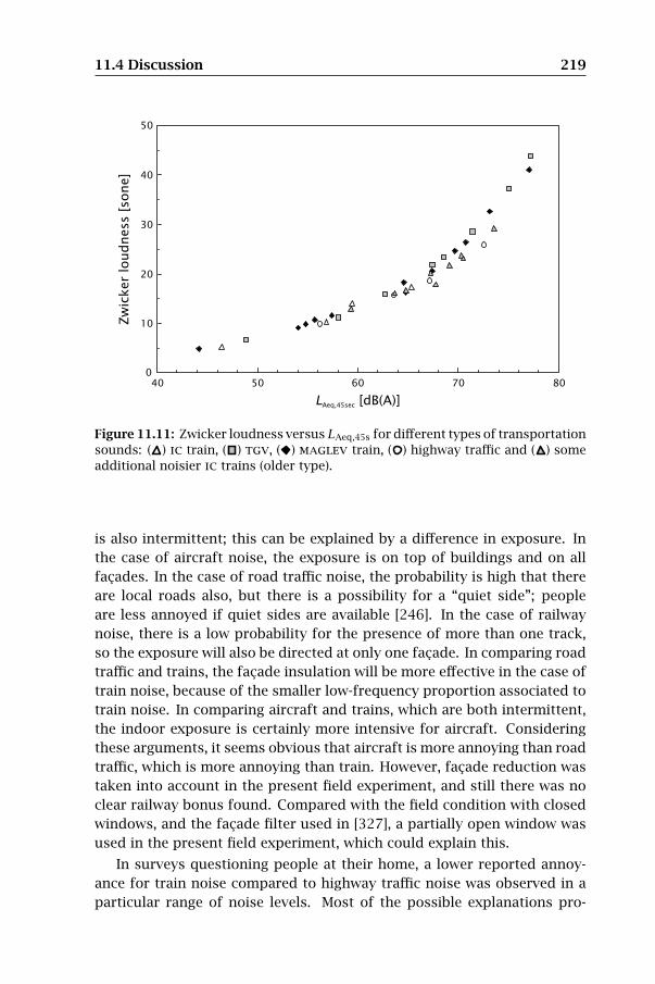
11.4 Discussion 219
0
10
20
30
40
50
40 50 60 70 80
Zw
icker
loudness [
sone]
LAeq,45sec [dB(A)]
Figure 11.11: Zwicker loudness versus LAeq,45s for different types of transportationsounds: ( ) ic train, ( ) tgv, ( ) maglev train, ( ) highway traffic and ( ) someadditional noisier ic trains (older type).
is also intermittent; this can be explained by a difference in exposure. In
the case of aircraft noise, the exposure is on top of buildings and on all
façades. In the case of road traffic noise, the probability is high that there
are local roads also, but there is a possibility for a “quiet side”; people
are less annoyed if quiet sides are available [246]. In the case of railway
noise, there is a low probability for the presence of more than one track,
so the exposure will also be directed at only one façade. In comparing road
traffic and trains, the façade insulation will be more effective in the case of
train noise, because of the smaller low-frequency proportion associated to
train noise. In comparing aircraft and trains, which are both intermittent,
the indoor exposure is certainly more intensive for aircraft. Considering
these arguments, it seems obvious that aircraft is more annoying than road
traffic, which is more annoying than train. However, façade reduction was
taken into account in the present field experiment, and still there was no
clear railway bonus found. Compared with the field condition with closed
windows, and the façade filter used in [327], a partially open window was
used in the present field experiment, which could explain this.
In surveys questioning people at their home, a lower reported annoy-
ance for train noise compared to highway traffic noise was observed in a
particular range of noise levels. Most of the possible explanations pro-

220 Noise Annoyance caused by High-speed Trains
posed in literature conflict with the fact that this railway bonus would be
observed in experiments based on single passages. We mention just a few.
The typical character of train noise and the concentration of the sound en-
ergy in short time intervals may be advantageous with regard to activity
disturbance. If the level is sufficiently low, the probability of noticing the
train noise is small compared to the probability of noticing the sound of
a continuous source. In addition to physical differences in the sound, the
“green image” of trains as a means of transportation may add to the accept-
ability of the source and thus increase the tolerance to its noise, that is as
long as train passages are not too frequent. However, a more recent hedo-
nic pricing study found that householders in Birmingham place a greater
value on reductions in railway noise than in road traffic noise [9]. Cross-
cultural studies have shown that a railway bonus is not universal [344],
which would favor the argument above. It has further been shown that the
bonus varies depending on the (multiple) exposure situation [62]. Based
on the above, only part of the effect is supposed to be visible in field ex-
periments such as the one reported of in this paper. Part of the effect is
precisely what is observed.
11.5 Conclusion
This study has shown that in an “at home” like context, noise annoyance
caused by different types of trains at the same average outdoor façade ex-
posure level is not significantly different. In particular, magnetic levitation
systems are not more annoying than conventional high speed trains, which
is in agreement with earlier research. Noise annoyance caused by conven-
tional trains was not found to be significantly lower than annoyance caused
by tgv’s or maglev trains at the same average façade exposure. Field sur-
veys have shown that for the same average sound level, railway noise causes
less annoyance or highly annoyed persons than highway traffic noise. Al-
though our field experiment included several factors that may contribute
to this effect, we could not observe it.
Chapter12
Auditory Distance Perception
and Temporal Aspects
12.1 Introduction
The physical distance between the source and the observer plays an im-
portant role in noise annoyance. As a consequence of propagation effects
such as geometrical spreading, the ground effect and air absorption, the
sound pressure level of a noise source decreases with increasing distance.
Noise produced by a source located further from an observer is therefore
often assessed as less annoying than noise produced by an identical source
that is located closer. However, other characteristics of noise, such as its
spectrum and temporal structure, are also influenced by these propagation
effects. In the previous chapter, we have shown that in the case of trans-
portation noise, the distance to the source explains a significant amount of
annoyance variance not accounted for by sound level (10-minute menus).
Based on an analysis of several social surveys on community response to
railway and road traffic noise, the authors in [223] concluded the same.
At close distance, the variance in train noise annoyance not explained
by sound pressure level may be due to the presence of vibration from the
railway track, caused by trains passing by [243, 223]. Providing a satis-
factory explanation for the variance in noise annoyance at larger distances
from the track is less easy. In [259], it is deduced from a laboratory ex-
periment that the extra variance in perceived train noise annoyance, above
the variance introduced by variations in sound pressure level, can not be
explained merely on the basis of the spectral content of the noise source.
It is suggested that characteristics of the temporal envelope of the noise,
e.g. the rise time, also contribute to annoyance. This is confirmed by the
experimental results from the previous chapter.

222 Auditory Distance Perception and Temporal Aspects
Noise annoyance may also be influenced by other factors related to the
perception of the noise source, such as the perceived distance between
the noise source and its observer. There can be little doubt about the fact
that vision plays a primary role in the perception of distance [347]. How-
ever, auditory distance perception may also be of importance if no visual
information on the noise source is available, which often is the case in an
at-home context. In this chapter, we will explore the acoustic variables that
may influence auditory distance perception, in the case the source is not
visible to the listener.
12.2 Perceived distance in an at-home context
The experiment described in the previous chapter happened to be a very
good occasion to investigate the perception of auditory distance in an at-
home context. For this, an extra question was asked during the conclud-
ing conventional listening test, for each of the experimental stimuli: “How
far from the house would you situate the origin of the traffic sound you
heard?”. The panelists had to write down their estimation of the distance
in meter (no master scaling). This direct method of scaling was chosen
in order for the panelists not to confuse these assessments with the noise
annoyance magnitude estimates. It is also the same method as earlier used
in [259] for moving noise sources such as trains passing by.
The distributions of distance assessments were strongly skewed to high
values: the arithmetic means were approximately two times greater than
the median distance assessment for each sound. Therefore, group data
was calculated as medians. Figure 12.1(a) shows the logarithm of the per-
ceived distance as a function of sound level (LAeq,45s). A strong negative
relationship is found (r = −0.90). For a given sound level, maglev train
sounds were perceived as slightly less distant than the tgv, ic and highway
sounds. Figure 12.1(b) shows the perceived distance as a function of the
physical distance. The relationship is weaker (r = 0.63). For a given physi-
cal distance, the spread in perceived distance was considerable, especially
at large physical distance.
These results suggest that perceived loudness (related to sound level)
was the main cue used for the distance assessments. To examine the possi-
ble influence of rise time, a multiple linear regression analysis was carried
out including only the train results, with perceived distance as dependent
variable, and sound level (dB(A)) and rise speed (dB(A)·s−1) as independent
variables. Table 12.1 summarizes the results. It is found that rise speed
indeed explains a significant part of the perceived distance variance for
trains, not accounted for by sound level.

12.2 Perceived distance in an at-home context 223
1.0
1.5
2.0
2.5
3.0
1.0 1.5 2.0 2.5
log
(perc
eiv
ed d
ista
nce)
[m]
10
log (distance) [m]10
(b)
1.0
1.5
2.0
2.5
3.0
40 50 60 70 80
log
(perc
eiv
ed d
ista
nce)
[m]
10
LAeq,45s [dB(A)]
(a)
Figure 12.1: Perceived distance (median assessment) in an at-home context, as afunction of (a) LAeq,45s and (b) physical distance, for different types of transporta-tion sounds: ( ) ic train, ( ) tgv, ( ) maglev train and ( ) highway traffic.
Table 12.1: Multiple regression analysis of acoustic variables on perceived dis-tance of train sounds in an at-home context.
Model Independent Coefficient Standardized t-valuefit (r 2) Variables coefficient
0.94 LAeq,45s [dB(A)] −0.025 −0.61 −7.18∗∗∗
Rise speed [dB(A)·s−1] −0.028 −0.41 −4.81∗∗∗
∗p < 0.05, ∗∗p < 0.01, ∗∗∗p < 0.001.
224 Auditory Distance Perception and Temporal Aspects
12.3 Perceived distance in a laboratory context
A second experiment was conducted in a laboratory setting. Data and
recordings were used which were collected in the framework of an envi-
ronmental impact assessment study conducted in the Brennerpas valley, a
mountainous region connecting Austria with Italy. The Brennerpas high-
way passes through this region from north to south. On some parts it is
located on a viaduct, on other parts noise barriers are present. A railway
and a district road also pass through this region, approximately paralell
to the highway. Furthermore, some local roads are present. The noise of
the Brennerpas highway and railway may be heard throughout most of the
valley, causing noise annoyance for its inhabitants. One hypothesis is that
high noise annoyance in this region could be caused by the highway or rail-
way sounding closer by compared to reality, due to the valley topology or
to particular meteorological conditions (e.g. unusual atmospheric temper-
ature profiles). The main goal of this experiment therefore was to compare
the auditory distance perception of a highway or railway in an alpine area
with the auditory distance perception of a highway or railway in the ref-
erence situation of a flat area without buildings. For this purpose, test
persons were asked to compare transportation sounds recorded in both
situations for perceived distance to the source, and to estimate the dis-
tance. In the next sections, we will discuss the experimental methodology
and results.
12.3.1 Experimental methodology
Location and equipment
The listening test was conducted in a quasi-anechoic chamber (well iso-
lated room with absorbing foam on walls and ceiling). The sounds were
played on a regular pc equiped with a high quality audio card, located in
an adjacent room, and presented to the test persons using a high quality
headphone. Furthermore, a subwoofer was placed in a corner of the ex-
perimental room, in order to achieve a good reproduction of frequencies
below 100 Hz. The test persons were seated in front of a screen, and had
a mouse and a numeric keyboard to their disposal for entering their an-
swers. The playback system was calibrated by placing a B&K artificial head
and torso at the position of the test person, by playing back pink noise and
equalizing the system to achieve a flat spectrum in 1/3-octave bands at the
ears of the binaural head. Equalization was done with software installed
on the playback pc. Figure 12.2 shows a test person performing a listening
test.

12.3 Perceived distance in a laboratory context 225
Figure 12.2: A test person performing a listening test.
Sound samples
A large set of binaural sound recordings were made during spring 2004 at
several locations in the Brennerpas valley, in cooperation with the Medical
University of Innsbruck. To select samples from the set of recordings, first
a selection of interesting locations was made using gis software. Locations
at varying distance from the highway (10 m to 3 km) and railway track (10 m
to 400 m) were chosen. Subsequently, recordings made at these locations
were listened to. For the highway noise, fragments with a duration of 30 s
were selected, in which no other disturbances are present. For the train
noise, high quality passages were selected. In total, 42 highway fragments
and 21 train passages were selected. For the reference recordings on flat
terrain without possible shielding by buildings, we used the highway and
ic train passage recordings, discussed in the previous chapter (train and
highway each at a distance of 25 m, 50 m, 100 m and 200 m).
Listening test outline
Menus of 8 highway noise fragments were composed, consisting of 7 frag-
ments recorded in alpine area (out of 42) and 1 reference fragment (out
of 4). These menus were not put together completely randomly. Care was
taken for that within the set of all menus, each couple of 2 alpine highway
fragments occurs together within one menu roughly the same number of

226 Auditory Distance Perception and Temporal Aspects
times, and also that each alpine fragment occurs together with each refer-
ence highway fragment roughly the same number of times. This procedure
was repeated for the train fragments.
Although the listening tests were performed for each test person sepa-
rately, the outline of the test was the same for all test persons. Firstly, the
test person had to sort a menu of 8 highway noise fragments, according
to his/her perceived distance to the highway. To make this task as simple
as possible, a series of comparisons of two fragments was presented (28
combinations in total), and the test person was only asked to select the
fragment which he/she thought sounded the closest. Both sounds could
be listened to as many times as needed. The actual sorting was then done
automatically using a sorting algorithm, based on the choices made by the
test person. Subsequently, the 8 fragments were presented once again to
the test person, this time individually and sorted according to the percep-
tion of the distance to the source (the test person was informed of this
sorting). The test person then had to give an estimate of the distance (in
meter) to the highway or railway track.
This procedure of sorting and distance estimation was repeated for a
train menu, and once again for a different highway menu. The evaluation
of one menu lasted about 30 minutes for most test persons.
Test panel
All together, 75 persons participated in the listening test, mainly students
and university staff. No special selection procedure was used to achieve a
representative test panel. The panel consisted of 39 male and 36 female
persons, with an average age of 27.5 year.
12.3.2 Results
Data quality analysis
The sorting of the noise fragments within a menu, according to perceived
auditory distance to the noise source, provides a means to assess the dif-
ficulty of the listening test. Consider the case of a comparison between
2 particular noise fragments. Both fragments will occur together in several
menus, and will as a consequence be compared by several test persons.
We may associate a score with the choice made by a particular test per-
son, defined as the percentage of test persons which were presented the
same comparison and made the same choice. If the particular comparison
is difficult, both choices will be made about the same number of times, and

12.3 Perceived distance in a laboratory context 227
we expect this score to be on average around 50 % (chance level). If the
particular comparison is easy, one of the fragments will be chosen most
of the time, and this score will be on average much higher than 50 %. The
performance of a test person on a single menu may then be assessed as
the average of all 28 comparisons made within the menu.
For the highway menus, we found that the average score was 88.97 %,
with a standard deviation of 5.78 %; for the train menus the average score
was 88.03 % with a standard deviation of 4.59 %. Both are well above chance
level, so we may conclude that the listening test was feasible. No significant
difference is found between the performance scores of the highway and
train menus, so we may conclude that it is equally difficult to compare
train noise and highway noise according to perceived auditory distance.
Distance estimation
Just like it was the case for the results of the experiment in an at-home
context, the distributions of distance assessments were strongly skewed
to high values; therefore the median estimated distance was calculated for
each sound fragment.
Figure 12.3(a) shows the logarithm of the perceived distance for the
highway fragments, as a function of sound level (LAeq,30s). A strong nega-
tive relationship is found (r = −0.94). No significant difference is found
between the fragments recorded in alpine area or on flat terrain. By con-
ducting a stepwise multiple linear regression analysis, factors related to the
spectral content (sharpness, spectrum centre of gravity) were not found to
explain a significant additional part of perceived distance variance. Fig-
ure 12.3(b) shows the logarithm of the perceived distance as a function of
the physical distance. The relationship is weaker (r = 0.69); for a given
physical distance, the spread in perceived distance is considerable. For
physical distances between 50 m and 200 m, the perceived auditory dis-
tance is the smallest for the highway noise recorded on flat terrain without
shielding.
Figure 12.4(a) shows the logarithm of the perceived distance for the rail-
way fragments, as a function of sound exposure level (ASEL). Compared to
the highway results, a somewhat less strong negative relationship is found
(r = −0.90). Again, no significant difference is found between the frag-
ments recorded in alpine area or on flat terrain. A multiple linear regres-
sion analysis (Table 12.2) revealed that rise speed of the noise of the train
passage explained a significant additional part of the variance in perceived
distance, not accounted for by sound level.

228 Auditory Distance Perception and Temporal Aspects
0.0
0.5
1.0
1.5
2.0
2.5
3.0
3.53.02.52.01.51.00.50.0
log
(perc
eiv
ed d
ista
nce)
[m]
10
log (distance) [m]10
(b)
0.0
0.5
1.0
1.5
2.0
2.5
3.0
40 50 70 80 9060
log
(perc
eiv
ed d
ista
nce)
[m]
10
LAeq,30s [dB(A)]
(a)
Figure 12.3: Perceived distance (median assessment) of highway noise in a labora-tory context, as a function of (a) LAeq,30s and (b) physical distance, for recordingsmade ( ) in alpine area and ( ) on flat terrain.
Table 12.2: Multiple regression analysis of acoustic variables on perceived dis-tance of train sounds in a laboratory context.
Model Independent Coefficient Standardized t-valuefit (r 2) Variables coefficient
0.88 ASEL [dB(A)] −0.042 −0.72 −8.62∗∗∗
Rise speed [dB(A)·s−1] −0.190 −0.33 −3.90∗∗
∗p < 0.05, ∗∗p < 0.01, ∗∗∗p < 0.001.

12.3 Perceived distance in a laboratory context 229
0.0
0.5
1.0
1.5
2.0
2.5
3.0
3.53.02.52.01.51.00.50.0
log
(perc
eiv
ed d
ista
nce)
[m]
10
log (distance) [m]10
(b)
0.0
0.5
1.0
1.5
2.0
2.5
3.0
60 70 80 90 100
log
(perc
eiv
ed d
ista
nce)
[m]
10
ASEL [dB(A)]
(a)
Figure 12.4: Perceived distance (median assessment) of railway noise in a labo-ratory context, as a function of (a) ASEL and (b) physical distance, for recordingsmade ( ) in alpine area and ( ) on flat terrain.

230 Auditory Distance Perception and Temporal Aspects
12.4 Conclusion
Based on the results of the two experiments discussed, it can be concluded
that for highway noise, which is continuous, as well as for railway noise,
which is intermittent, the perceived auditory distance is mainly determined
by sound pressure level. However, railway noise perceived auditory dis-
tance is also significantly influenced by rise time; the temporal aspect there-
fore seems to play a role in distance perception.
As it was already mentioned in Chapter 10, this may have an influence
on noise annoyance. A hypothesis could be that the chance an intermit-
tent sound is noticed is higher if the perceived auditory distance is short,
and a sound may only be annoying if it is noticed. One of the possible
implications would then be that noise abatement measures solely aimed at
reducing the sound pressure level, such as noise barriers, are less effective
for railway noise. However, to confirm this hypothesis, more research will
be needed.
Conclusions and Perspectives
In this work, models and methodologies to introduce the temporal aspect
into the study of our sonic environment have been developed. Road and
railway traffic, which are the main sources of noise in urban and rural envi-
ronment, received the focus. The achievements fit well within the current
soundscape approach to environmental noise, in which the basic principle
states that the perception of our sonic environment is influenced by all
other environmental aspects, and by the state of mind of the observer. In
this holistic vision, the positive as well as the negative aspects of our sonic
environment have been considered.
Models to simulate and predict temporal characteristics of sound are a
first and necessary step to introduce the temporal aspect into environ-
mental soundscape research. However, current traffic noise prediction
is mainly focused on energy equivalent sound pressure levels. Traffic is
hereby modeled as a stationary flow of vehicles with a constant speed.
Therefore, in Part I of this work, a model for the prediction of time-varying
road traffic noise was developed. A microsimulation traffic model was cou-
pled with a single-vehicle road traffic noise emission model (Nord 2000 &
Harmonoise), and a fast and efficient object precise beam tracing propaga-
tion model.
This dynamic noise prediction model allows drawing maps of a simu-
lated traffic situation in built-up area, showing various descriptors for the
impact of temporal aspects on the soundscape. Furthermore, it is possi-
ble to assess the impact of traffic management measures, such as the use
of traffic light timing or traffic re-routing, on the temporal characteristics
of the soundscape. In Chapter 2, the model was validated on a part of
Gentbrugge, a suburban area near Ghent, and in general a good agreement
with measurements was found. Scenario calculations for this case study
showed that minor changes in traffic (possibly caused by flow management)
have a much larger effect on the soundscape than expected on the bases
of average emission and immission mapping.
In Chapter 3, the variation in noise immission in the vicinity of inter-
sections, caused by the typical deceleration and acceleration profiles of
vehicles, was studied. Furthermore, a methodology to adjust classic traffic
noise prediction models for these time-depending phenomena which in-

232 Conclusions and Perspectives
fluence energy equivalent sound pressure levels was outlined. A number
of simple intersection scenarios were considered, in which only traffic de-
mand, composition and turning rate were varied. This somewhat limited
the applicability of the results. However, it was pointed out that in a typical
real life study area, the variation in intersection types is not very large, so
the methodology desribed in Chapter 3 could easily be used to study the
typical intersections in the study region, and to extrapolate the results to
the whole network under study.
A second prerequisite for the introduction of the temporal aspect are
suitable physical indicators, which are able to grasp the special characteris-
tics of a time-varying soundscape, and which have a clear relation to human
perception. Most of the noise measures currently in use, such as average
or percentile levels, do not consider the time pattern of sound. Therefore,
a search for a novel soundscape indicator which summarizes its temporal
structure was undertaken in Part II of this work.
It was already known that 1/f characteristics, related to dynamic and
complex systems, can be found in music, and that a clear relation exists
with musical preference. In Chapter 5, it was shown that a 1/f character-
istic can also be found in the temporal envelope of many natural, rural and
urban soundscapes. A link with the possible self-organized criticality of
the complex systems that form the underlying sources of the soundscape
was drawn. This brought us to propose a novel indicator for the temporal
structure of environmental soundscapes in Chapter 6, based on the statis-
tical similarity of the temporal structure of the soundscape with that of
music. More specificly, the proposed ml indicator measures the fuzzy cor-
respondence of the slope and deviation from a straight line of the spectral
density of the temporal envelope of the soundscape, with the typical slopes
and deviations from a straight line found in music.
A small-scale survey indicated that the ml characteristic did not corre-
late well with the feeling that the environmental noise sounds like music,
mainly because few subjects could imagine urban noise to be music. On
the contrary, there seemed to be a clearer relation to the soundscape being
neither chaotic nor boring. If anything, the presented ml indicator sheds
new light on how soundscape quality might be assessed in an objective
way. By using the analogy with music, the indicator follows more closely
the original ideas behind soundscape research. Based on this, we argue
that the proposed indicator is a good candidate for describing and cate-
gorizing soundscape temporal structure, and can be used in addition to
loudness and spectral-quality indicators (sharpness, roughness).
There is an obvious need for further analyses of the relation between
this objective indicator for temporal structure and the more subjective
evaluation of environmental soundscape quality by active participants. In

233
Chapter 7, it is argued that to scan the fundamental dimensions of per-
ceived soundscape quality, it may be necessary to use sound without mean-
ing. For this purpose, a new method for creating artificial soundscapes with
reduced detail in meaning, and with flexible temporal characteristics was
introduced, based on the concept of swarm intelligence. This model may
be used in listening experiments in which it is the goal to find the most
suitable soundscape to a given environment, and to extract the associated
physical characteristics.
The study of the sonic environment of urban parks or squares and natu-
ral or rural areas probably is the field of research in which the soundscape
vision adds the most value. As an application of the concepts introduced in
this work, a particular type of soundscape, the quiet area, was considered
in Part III of this work. Because of the positive psychological restoring ef-
fect quiet areas may have on people visiting it, their preservation has been
subscribed in the EC environmental noise directive, and in the policy inten-
tions of many countries. Nevertheless there is little scientific knowledge
on how to characterize such areas and possibly grant quality labels.
In Chapter 9, a literature study with focus on soundscape and (mental)
health related aspects showed that, to characterize quiet areas, a multi-
criteria approach is appropriate, including an assessment of the temporal
structure of the quiet area soundscape. A shortlist of possibly useful indi-
cators was concretized and tested on a typical quiet rural soundscape and
for comparison also on an urban area. Finally, a multi-criteria assessment
of quiet rural soundscape quality was proposed. Quality levels were de-
rived for this particular context, but could probably be extended to other
context easily.
Next to its main advantages in the positive field of psychological restora-
tion, research embracing the soundscape vision may also lead to a better
understanding of the processes that lead to noise annoyance. In the last
part of this work, an ecologically valid field experiment was discussed,
which incorporated the temporal aspect explicitly into the design. The
extreme cases of highway traffic noise, which is continuous, and railway
noise, which is intermittent, were considered. A difference in annoyance
between both is incorporated in the noise legislation in several countries,
mostly based on social survey data. However, no evidence which supports
this so called railway bonus was found in our field experiment. On the
other hand, temporal effects were indeed found to influence perceived an-
noyance. It was shown that temporal aspects of noise may cause the source
to sound closer by or further away, which may explain their influence on
noise annoyance. In particular, it was shown that the rise time of the sound
of a train passing by has a significant influence on perceived distance to
the track.
234 Conclusions and Perspectives
The field of research covered by this work is very broad, which is re-
flected in the close collaboration with experts in the fields of traffic en-
gineering, computer science, psychology and medicine. This work con-
tributes to the understanding of (the perception of) temporal aspects in
urban, rural and natural soundscapes. As its main innovative aspects, this
work
• shows that accounting for the temporal aspect in noise mapping is
feasible, but that appropriate indicators for the temporal structure
have to be employed,
• links characteristics of complex systems, and in particular the fluctu-
ations in loudness and pitch as found in music, with (the perception
of) urban, rural and natural soundscapes,
• broadens the way quiet area quality is assessed, stressing the need
for acoustic as well as non-acoustic factors to be taken into account,
and
• takes an initiative to introduce the temporal aspect into the study of
the emergence of noise annoyance in an at-home context.
Although the energy equivalent sound pressure level will most probably al-
ways be the main indicator to assess the quality of our sonic environment
and to predict noise annoyance, there is a growing awareness of the fact
that there is more to noise than level. The increasing interest in sound-
scape research shows that it is possible to bend environmental acoustics
into a positive field of study. It is the author’s hope that this work may con-
tribute to a better understanding of the temporal aspects of environmental
soundscapes and their relation to human perception.

Appendices


AppendixA
Calculation of Music-likeness
A.1 Spectrum of fluctuations
The calculation procedure departs from a time series Xn (n = 1 . . . N),
which represents a discretized temporal envelope associated to the sound-
scape under study. Throughout this work, several quantities have been
used for the temporal envelope:
(L) The A-weighted sound pressure level (e.g. LAeq,1s);
(Z) The instantaneous pitch;
(N) The instantaneous loudness;
(V) The wind velocity;
For standardization purposes, it is proposed to use LAeq,1s, as it is the
quantity that is most easily measured or calculated.
The power spectrum SX(f ) of this time series is then calculated using an
fft, applying a rectangular window with the same size as the time series,
and removing the dc term. The following matlab code may be used:
s = fft(x); % calculating fourier spectrum
s = s(1 : (N/2)); % removing symmetric part
s = abs(s.∗ conj(s)); % calculating power spectrum
s = s(2 : end); % removing DC− term
The total length of the time series determines the lower frequency bound
of the resulting spectrum, the sampling frequency determines the upper
bound. As we are interested in correlations between the (sound) events over

238 Calculation of Music-likeness
–3
–2
–1
0
1
2
3
4
–3.5 –3.0 –2.5 –2.0 –1.5 –1.0 –0.5 0.0
log
()
[a.u
.]1
0X
S
log ( ) [Hz]10 f
Figure A.1: Calculation of a linear fit of SX in the interval [0.002 Hz, 0.2 Hz].
longer timescales (up to several minutes), the temporal envelope should
be measured (simulated) during a sufficiently long period. A minimum
of 15 minutes is proposed, which will result in a lower bound of at least
2/(15 · 60) = 0.002 Hz.
A.2 Music-likeness
Subsequently, the spectrum is smoothed to 12 data points per octave band.
For this, the frequency axis is subdivided in 1/12th octave intervals, and
the average value of SX(f ) in each interval is calculated (or interpolated
if necessary). This will result in an equidistant spacing of the data points,
when the spectrum is plotted on a log-log scale, which is necessary to make
a correct linear regression (see Figure A.1). A straight line is fitted through
the resulting data points in the interval [0.002 Hz, 0.2 Hz] on a log-log scale,
and the slope α and the rms value ǫ of the fitting error are calculated.
Finally, the fuzzy correspondence of the parameters α and ǫ to typical
values found in music is calculated using Eq. 4.19, with the distributions
(Eq. 4.16) extracted from analysing several music fragments (see Chapter 6):
σα,1 = 0.488 σα,2 = 0.305 ρα = −0.931
σǫ,1 = 10.000 σǫ,2 = 0.069 ρǫ = 0.437

AppendixB
Soundscape Fragments
A large number of soundscape recordings or music fragments have been
referenced in this work using a label. In this appendix, an overview is
presented, which provides the reader for a quick reference. For the record-
ings, where possible, the location (in Dutch) is mentioned or a description
is given.
Rural soundscapes (Recorded from autumn 1997 to spring 1998)
R1–R6 Zwin (Knokke Heist)
R7–R12 Lampernisse
R13 E40 highway at far distance
R14 Train passing by at far distance
Urban soundscapes recorded in Ghent (Session 1, Spring 2002)
A description of the locations can be found in Table 5.2.
G1 Begijnhof
G2 Bourgoyen
G3 Brabantdam
G4 Graslei
G5 Korenmarkt
G6 Kouter
G7 Mageleinstraat
G8 Nieuwe Wandeling
G9 P. de Smet de Naeyerplein
G10 Prinsenhof
G11 Veldstraat
G12 Watersportbaan

240 Soundscape Fragments
Urban soundscapes recorded in Ghent (Session 2, Autumn 2002)
U1 Bourgoyen
U2 Brabantdam
U3 Citadelpark
U4 Graslei
U5 Korenmarkt (1)
U6 Korenmarkt (2)
U7 Kouter
U8 Lange Violettestraat
U9 Mageleinstraat
U10 Nieuwe Wandeling
U11 P. de Smet de Naeyerplein
U12 Prinsenhof
U13 Rabot
U14 Veldstraat
U15 Watersportbaan
U16 Gentbrugge location 1 (Figure 2.3)
U17 Gentbrugge location 2
U18 Gentbrugge location 3
U19 Gentbrugge location 4
U20 Gentbrugge location 5
U21 Gentbrugge location 6
U22 Access road to highway
U23 E40 highway at close distance
U24 R4 highway at close distance
Natural Soundscapes
N1 Fountain
N2 Birds (dawn chorus) in Belgian garden
N3 Sea waves breaking on coastal rocks
N4 Birds singing in Cornwall, South West England
N5 Wind in trees
Noise and Speech
W White noise
S Radio broadcast (“Eeuwfeest”, 15/10/2000, Flemish Radio 1)

241
Music
M1 Abbey Road – The Beatles
M2 Dark Side of the Moon – Pink Floyd
M3 Far East Suite – Duke Ellington Orchestra
M4 Giant Steps – John Coltrane
M5 Kind of Blue – Miles Davis
M6 The Doors – The Doors
M7 Adagio for strings – S. Barber
M8 Appalachian Springs – A. Copland
M9 Bolero – M. Ravel
M10 Brandenburg Concerto No. 1 – J. S. Bach
M11 Orchestral Suite No. 2 – J. S. Bach
M12 Orchestral Suite No. 3 – J. S. Bach
M13 Piano Concerto No. 2 – S. Rachmaninov
M14 Requiem – W. A. Mozart
M15 The Four Seasons – A. Vivaldi

Bibliography
[1] Traffic flow theory: A state-of-the-art report. Technical report, Transporta-
tion Research Board, US Department of Transportation, Washington DC,
USA, Dec. 1997.
[2] S. Algers, E. Bernauer, M. Boero, L. Breheret, C. Di Taranto, M. Dougherty,
K. Fox, and J.-F. Gabard. Review of micro-simulation models. SMARTEST
Project Deliverable D3, ITS, University of Leeds, UK, Mar. 1998.
[3] O. Axelsson, B. Berglund, and M. E. Nilsson. Soundscape assessment. J.
Acoust. Soc. Am., 117(4):2591–2592, 2005.
[4] K. W. Axhausen and T. Garling. Activity-based approaches to travel anal-
ysis - Conceptual frameworks, models, and research problems. Transport
Reviews, 12(4):323–341, 1992.
[5] T. Bäck. Evolutionary Algorithms in Theory and Practice. Oxford University
Press, New York, USA, 1996.
[6] R. Badii and A. Politi. Complexity: Hierarchical Structures and Scaling in
Physics. Number 6 in Cambridge Nonlinear Science Series. Cambridge Uni-
versity Press, Cambridge, UK, 1997.
[7] H. Baher. Analog & Digital Signal Processing. John Wiley & Sons, Inc., Chich-
ester, West Sussex, UK, second edition, 2001.
[8] P. Bak, C. Tang, and K. Wiesenfeld. Self-organized criticality: An explanation
of 1/f noise. Physical Review Letters, 59(4):381–384, 1987.
[9] I. J. Bateman, B. H. Day, and L. I. The valuation of transport-related noise in
Birmingham. Technical report, Department of Transport, London, UK, Sept.
2004.
[10] J. Beaumont, B. Robin, and C. Semidor. Event descriptors for qualifying the
urban sound environment. In Proceedings of Forum Acusticum, Budapest,
Hungary, Aug. 2005.
[11] G. Beni and U. Wang. Swarm intelligence in cellular robotic systems. In Pro-
ceedings of the NATO Advanced Workshop on Robots and Biological Systems,
Il Ciocco, Tuscany, Italy, 1989.
[12] M. Bérengier. Acoustical impact of traffic flowing equipments in urban area.
In Proceedings of Forum Acusticum, Sevilla, Spain, Sept. 2002.
[13] B. Berglund. Quality assurance in environmental psychophysics. In S. J.
Bolanowski and G. A. Gescheider, editors, Ratio Scaling of Psychological
Magnitudes — In Honor of the Memory of S. S. Stevens. Erlbaum, Hillsdale,
New Jersey, USA, 1991.

244 Bibliography
[14] B. Berglund. The role of loudness as guide for community noise. In Pro-
ceedings of The 20th International Congress on Noise Control Engineering
(Inter·noise), Sydney, Australia, Dec. 1991.
[15] B. Berglund, U. Berglund, and T. Lindvall. A study of response criteria in
populations exposed to aircraft noise. J. Sound. Vib., 41(1):33–39, 1975.
[16] B. Berglund, P. Hassmén, and R. F. S. Job. Sources and effects of low-
frequency noise. J. Acoust. Soc. Am., 99(5):2985–3002, 1996.
[17] B. Berglund, P. Hassmén, and A. Preis. Annoyance and spectral contrast are
cues for similarity and preference of sounds. J. Sound. Vib., 250(1):53–64,
2002.
[18] B. Berglund, T. Lindvall, and D. H. Schwela, editors. Guidelines for Commu-
nity Noise. World Health Organization, Geneva, Switzerland, Apr. 1999.
[19] B. Berglund and M. E. Nilsson. Loudness of combined noises derived from
singular and concurrent community noises. In Proceedings of The 16th Inter-
national Congress on Acoustics (ICA), Seattle, Washington, USA, June 1998.
[20] B. Berglund and M. E. Nilsson. An attempt to capture the perceived sound-
scape. In Proceedings of the International Symposium on Noise Pollution and
Health (NOPHER), Cambridge, UK, Apr. 2001.
[21] B. Berglund and A. Preis. Is perceived annoyance more subject-dependent
than perceived loudness? Acustica, 83(2):313–319, 1997.
[22] R. Berto. Exposure to restorative environments helps restore attentional
capacity. Journal of Environmental Psychology, 25(3):249–259, 2005.
[23] F. Besnard, J. Lelong, S. Doisy, and V. Steimer. Updating the vehicle noise
emission values used in French traffic noise prediction models. In Pro-
ceedings of The 28th International Congress on Noise Control Engineering
(Inter·noise), Fort Lauderdale, Florida, USA, Dec. 1999.
[24] J. M. Bishop. Stochastic searching networks. In Proceedings of the 1st IEEE
International Conference on Artificial Neural Networks, pages 329–331, Lon-
don, UK, Oct. 1989.
[25] J. M. Bishop and P. Torr. The stochastic search network. In R. Linggard, D. J.
Myers, and C. Nightingale, editors, Neural Networks for Vision, Speech and
Natural Language, volume 1 of BT Telecommunication Series, pages 370–
387. Springer, New York, USA, 1992.
[26] E. A. Björk. Effects of inter-stimulus interval and duration of sound elements
on annoyance. Acta Acustica united with Acustica, 88(1):104–109, 2002.
[27] T. M. Blackwell and P. Bentley. Don’t push me! Collision-avoiding swarms. In
Proceedings of the 2002 IEEE World Congress on Computational Intelligence,
Honolulu, Hawaii, USA, May 2002.
[28] T. M. Blackwell and P. Bentley. Improvised music with swarms. In Proceedings
of the 2002 IEEE World Congress on Computational Intelligence, Honolulu,
Hawaii, USA, May 2002.

245
[29] J. W. D. Boddy, R. J. Smalley, P. S. Goodman, J. E. Tate, M. C. Bell, and A. S.
Tomlin. The spatial variability in concentrations of a traffic-related pollu-
tant in two street canyons in York, UK — Part II: The influence of traffic
characteristics. Atmospheric Environment, 39(17):3163–3176, 2005.
[30] H. F. Boersma. Characterization of the natural ambient sound environ-
ment: Measurements in open agricultural grassland. J. Acoust. Soc. Am.,
101(4):2104–2110, 1997.
[31] E. Bonabeau, M. Dorigo, and G. Theraulaz. Swarm Intelligence: From Natural
to Artificial Systems. Santa Fe Institute Studies in the Sciences of Complexity.
Oxford University Press, New York, USA, 1999.
[32] G. L. Bonvallet. Levels and spectra of noise in industrial and residential areas.
J. Acoust. Soc. Am., 21(4):463, 1949.
[33] J. P. Boon and O. Decroly. Dynamical systems theory for music dynamics.
Chaos, 5(3):501–508, 1995.
[34] J. P. Boon and I. Prigogine. Le temps dans la forme musicale. In E. Darbel-
lay, editor, Le Temps et la Forme, pages 139–164. Editions DROZ, Geneva,
Switzerland, 1998.
[35] H. Borst. URBIS: Instrument for local environmental survey. In Proceedings of
The 29th International Congress on Noise Control Engineering (Inter·noise),
Nice, France, Aug. 2000.
[36] D. Botteldooren and B. De Coensel. Quality assessment of quiet areas: A
multi-criteria approach. In Proceedings of The 6th European Conference on
Noise Control (Euronoise), Tampere, Finland, May 2006.
[37] D. Botteldooren, B. De Coensel, and T. De Muer. Music in the urban sound-
scape? Lay language paper prepared for The 1st Pan-American/Iberian Meet-
ing on Acoustics, Cancun, Mexico, Dec. 2002. Available online at the ASA
World Wide Press Room: http://www.acoustics.org/press/144th/.
[38] D. Botteldooren, B. De Coensel, and T. De Muer. 1/f dynamics in the urban
soundscape. J. Acoust. Soc. Am., 112(5):2436, 2002.
[39] D. Botteldooren, B. De Coensel, and T. De Muer. The effect of traffic flows
on urban soundscape dynamics and how to analyze it. In Proceedings of The
18th International Congress on Acoustics (ICA), Kyoto, Japan, Apr. 2004.
[40] D. Botteldooren, B. De Coensel, and T. De Muer. The temporal structure of
the urban soundscape. In Proceedings of CFA/DAGA’04, Strasbourg, France,
Mar. 2004.
[41] D. Botteldooren, B. De Coensel, and T. De Muer. The temporal structure of
urban soundscapes. J. Sound. Vib., 292(1–2):105–123, 2006.
[42] D. Botteldooren, B. De Coensel, T. De Muer, B. Berglund, M. Nilsson, and
P. Lercher. Experimental investigation of noise annoyance caused by high-
speed trains. In Proceedings of The 12th International Congress on Sound
and Vibration (ICSV), Lisbon, Portugal, July 2005.

246 Bibliography
[43] D. Botteldooren, S. Decloedt, J. Bruyneel, and S. Pottie. Characterisation of
quiet areas: subjective evaluation and sound level indices. In Proceedings of
Forum Acusticum, Berlin, Germany, Mar. 1999.
[44] D. Botteldooren and A. Verkeyn. On the meaning of noise annoyance modi-
fiers: A fuzzy set theoretical approach. Acta Acustica united with Acustica,
88(2):239–251, 2002.
[45] D. Botteldooren, A. Verkeyn, and P. Lercher. Noise annoyance modeling
using fuzzy rule based systems. Noise and Health, 4(15):27–44, 2002.
[46] D. Botteldooren, A. Verkeyn, and P. Lercher. A fuzzy rule based framework
for noise annoyance modeling. J. Acoust. Soc. Am., 114(3):1487–1498, 2003.
[47] D. Boyce. Forecasting travel on congested urban transportation networks:
Review and prospects for network equilibrium models. In Proceedings of the
5th Triennial Symposium on Transportation Analysis (TRISTAN V), Le Gosier,
Guadeloupe, French West Indies, June 2004.
[48] M. Brackstone and M. McDonald. Car-following: a historical review. Trans-
portation Research Part F, 2(4):181–196, 1999.
[49] G. Brambilla and L. Maffei. Responses to noise in urban parks and in rural
quiet areas. Acta Acustica united with Acustica, 92(6), 2006.
[50] A. L. Brown. Towards criteria for outdoor soundscapes. In Proceedings of
ICBEN, Rotterdam, The Netherlands, June 2003.
[51] D. Burraston, E. Edmonds, D. Livingstone, and E. R. Miranda. Cellular au-
tomata in MIDI based computer music. In Proceedings of the International
Computer Music Conference, Miami, Florida, USA, 2004.
[52] C. Caldwell and V. S. Johnston. Tracking a criminal suspect through “face-
space” with a genetic algorithm. In Proceedings of the 4th International Con-
ference on Genetic Algorithms, pages 416–421, San Diego, California, USA,
1991.
[53] S. Camazine, J.-L. Deneubourg, N. R. Franks, J. Sneyd, G. Theraulaz, and
E. Bonabeau. Self-organization in Biological Systems. Princeton University
Press, Princeton, New Jersey, USA, 2003.
[54] R. E. Chandler, R. Herman, and E. W. Montroll. Traffic dynamics: Studies in
car following. Operations Research, 6(2):165–184, 1958.
[55] M. Y. Choi and H. Y. Lee. Traffic flow and 1/f fluctuations. Physical Review
E, 52(6):5979–5984, 1995.
[56] D. Chowdhury, L. Santen, and A. Schadschneider. Statistical physics of vehic-
ular traffic and some related systems. Phys. Rep., 329(4–6):199–329, 2000.
[57] D. Chowdhury and A. Schadschneider. Self-organisation of traffic jams in
cities: Effects of stochastic dynamics and signal periods. Physical Review E,
59(2):R1311–R1314, 1999.
[58] S. Clar, B. Drossel, and F. Schwabl. Forest fires and other examples of self-
organized criticality. Journal of Physics: Condensed Matter, 8(37):6803–
6824, 1996.

247
[59] M. Clerc. Particle Swarm Optimization. ISTE Publishing Company, London,
UK, 2006.
[60] A. Colorni, M. Dorigo, and V. Maniezzo. Distributed optimization by ant
colonies. In F. Varela and P. Bourgine, editors, Proceedings of the 1st Eu-
ropean Conference on Artificial Life (ECAL), pages 134–142, Paris, France,
1991.
[61] M. Cremer and J. Ludwig. A fast simulation model for traffic flow on the
basis of boolean operations. Math. Comput. Simul., 28(4):297–303, 1986.
[62] C. Cremezi, P. E. Gautier, J. Lambert, and P. Champelovier. Annoyance due
to combined noise sources — advanced results. In Proceedings of The 17th
International Congress on Acoustics (ICA), Rome, Italy, Sept. 2001.
[63] http://www.cresson.archi.fr. Cresson is the leading international institute
for research on acoustic design.
[64] M. J. Crocker. Rating measures, descriptors, criteria and procedures for
determining human response to noise. In M. J. Crocker, editor, Encyclopedia
of Acoustics, volume 2, chapter 80, pages 943–965. John Wiley & Sons, Inc.,
New York, USA, 1997.
[65] CRTN — Calculation of road traffic noise. Department of Transport, Welsh
Office, London, 1988.
[66] J. Davidsen and H. G. Schuster. 1/fα noise from self-organized critical mod-
els with uniform driving. Physical Review E, 62(5):6111–6115, 2000.
[67] M. de Berg, M. van Kreveld, M. Overmars, and O. Schwarzkopf. Computational
Geometry: Algorithms and Applications. Springer-Verlag, Berlin, Germany,
1997.
[68] B. De Coensel. Digitale signaalverwerking voor analyse van geluidsland-
schappen (digital signal processing for soundscape analysis) (in dutch). Mas-
ter’s thesis, Departement of Information Technology, Faculty of Applied Sci-
ences, Ghent University, Belgium, June 2002.
[69] B. De Coensel, D. Botteldooren, and T. De Muer. 1/f noise in rural and urban
soundscapes. Acta Acustica united with Acustica, 89(2):287–295, 2003.
[70] B. De Coensel, D. Botteldooren, and T. De Muer. Classification of sound-
scapes based on their dynamics. In Proceedings of ICBEN, Rotterdam, The
Netherlands, June 2003.
[71] B. De Coensel, T. De Muer, and D. Botteldooren. Onderzoek dynamiek
stedelijk geluidslandschap door wegverkeer. Geluid, 27(2):55–58, 2004.
[72] B. De Coensel, T. De Muer, I. Yperman, and D. Botteldooren. The influence of
traffic flow dynamics on urban soundscapes. Applied Acoustics, 66(2):175–
194, 2005.
[73] B. De Coensel, F. Vanhove, S. Logghe, I. Wilmink, and D. Botteldooren. Noise
emission corrections at intersections based on microscopic traffic simula-
tion. In Proceedings of The 6th European Conference on Noise Control (Eu-
ronoise), Tampere, Finland, May 2006.

248 Bibliography
[74] B. de Greve. Polygonale bundeltrekker voor akoestische simulaties (polyg-
onal beamtracer for acoustic simulations) (in dutch). Master’s thesis, De-
partement of Information Technology, Faculty of Applied Sciences, Ghent
University, Belgium, June 2003.
[75] R. G. de Jong. Beoordelingsmethode stiltegebieden, deelrapport beleving-
sonderzoek. TNO report 98.027, Leiden, The Netherlands, May 1998.
[76] P. De Los Rios and Y.-C. Zhang. Universal 1/f noise from dissipative self-
organised criticality models. Physical Review Letters, 82(3):472–475, 1999.
[77] K. De Meyer. Foundations of Stochastic Diffusion Search. PhD thesis, Depart-
ment of Cybernetics, University of Reading, UK, Jan. 2004.
[78] T. De Muer. Policy Supporting Tools for Urban Noise Assessment. PhD thesis,
Department of Information Technology, Ghent University, Belgium, Sept.
2005.
[79] T. De Muer, D. Botteldooren, B. De Coensel, B. Berglund, M. E. Nilsson, and
P. Lercher. A model for noise annoyance based on notice-events. In Pro-
ceedings of The 2005 Congress and Exposition on Noise Control Engineering
(Inter·noise), Rio de Janeiro, Brazil, Aug. 2005.
[80] P. de Vos, M. Beuving, and E. Verheijen. Harmonoise — Harmonised Accurate
and Reliable Methods for the EU Directive on the Assessment and Manage-
ment Of Environmental Noise. Final Technical Report — Deliverable 4 of the
Harmonoise project HAR7TR-041213-AEAT03, Feb. 2005.
[81] J. Deprez. Ieder stadsdeel zijn geluidsklimaat (a soundscape for each part of
town) (in dutch). Master’s thesis, Departement of Information Technology,
Faculty of Applied Sciences, Ghent University, Belgium, June 2004.
[82] V. Desarnaulds, G. Monay, and A. Carvalho. Noise reduction by urban traffic
management. In Proceedings of The 18th International Congress on Acoustics
(ICA), Kyoto, Japan, Apr. 2004.
[83] I. S. Diggory and B. Oakes. Computer simulation model for the prediction of
traffic noise levels. Applied Acoustics, 13(1):19–31, 1980.
[84] M. Dorigo and T. Stützle. Ant Colony Optimization. The MIT Press, Cam-
bridge, Massachusetts, USA, 2004.
[85] D. Dubois and S. David. A cognitive approach of urban soundscapes. In
Proceedings of Forum Acusticum, Berlin, Germany, Mar. 1999.
[86] D. Dubois and C. Guastavino. The ideal urban soundscape: investigating the
sound quality of French cities. In Proceedings of The 6th European Confer-
ence on Noise Control (Euronoise), Tampere, Finland, May 2006.
[87] D. Dubois, C. Guastavino, and V. Maffiolo. A cognitive approach to sound-
scape — Acoustic phenomena between “noise(s)” and “sound(s)”. In Proceed-
ings of CFA/DAGA’04, Strasbourg, France, Mar. 2004.
[88] D. Dubois and H. Prade, editors. Fundamentals of Fuzzy Sets, volume 7 of
The Handbooks of Fuzzy Sets Series. Springer, 1st edition, 2000.
249
[89] A. E. Eiben and J. E. Smith. Introduction to Evolutionary Computing. Natural
Computing Series. Springer-Verlag, Heidelberg, Germany, 2003.
[90] W. Ellermeier, M. Eigenstetter, and K. Zimmer. Psychoacoustic correlates of
individual noise sensitivity. J. Acoust. Soc. Am., 109(4):1464–1473, 2001.
[91] W. Ellermeier, A. Zeitler, and H. Fastl. Impact of source identifiability on
perceived loudness. In Proceedings of The 18th International Congress on
Acoustics (ICA), Kyoto, Japan, Apr. 2004.
[92] W. Ellermeier, A. Zeitler, and H. Fastl. Predicting annoyance judgments from
psychoacoustic metrics: Identifiable versus neutralized sounds. In Proceed-
ings of The 33rd International Congress and Exposition on Noise Control En-
gineering (Inter·noise), Prague, Czech Republic, Aug. 2004.
[93] Directive 2002/49/EC of the European Parliament and of the Council relating
to the assessment and management of environmental noise, Jun. 2002.
[94] D. F. Ettema and H. J. P. Timmermans, editors. Activity-based approaches to
travel analysis. Elsevier Science Ltd., Kidlington, Oxford, UK, 1997.
[95] K. Falconer. Fractal Geometry: Mathematical Foundations and Applications.
John Wiley & Sons, Inc., Chichester, West Sussex, UK, 1999.
[96] H. Fastl. Railway bonus and aircraft malus: Subjective and physical evalua-
tion. In Proceedings of the 5th International Symposium on Transport Noise
and Vibration, St. Petersburg, Russia, June 2000.
[97] H. Fastl. Neutralizing the meaning of sound for sound quality evaluations.
In Proceedings of The 17th International Congress on Acoustics (ICA), Rome,
Italy, Sept. 2001.
[98] H. Fastl. Features of neutralized sounds for long term evaluation. In Pro-
ceedings of Forum Acusticum, Sevilla, Spain, Sept. 2002.
[99] H. Fastl and G. Gottschling. Subjective evaluation of noise immissions from
Transrapid. In Proceedings of The 25th International Congress on Noise Con-
trol Engineering (Inter·noise), Liverpool, UK, July 1996.
[100] B. Favre. Noise at the approach to traffic lights: Result of a simulation pro-
gramme. J. Sound. Vib., 58(4):563–578, 1978.
[101] O. Fégeant. Wind-induced vegetation noise. Part II: Field measurements.
Acustica, 85(2):241–249, 1999.
[102] T. Feng, C. Xiao-hong, and L. Tan-feng. A social survey on the effects of
high-speed maglev noise on residents in Shangai. In Proceedings of The
2005 Congress and Exposition on Noise Control Engineering (Inter·noise), Rio
de Janeiro, Brazil, Aug. 2005.
[103] S. Fidell, S. Teffeteller, R. Horonjeff, and D. M. Green. Predicting annoyance
from detectability of low-level sounds. J. Acoust. Soc. Am., 66(5):1427–1434,
1979.
[104] A. Fiebig and B. Schulte-Fortkamp. The importance of the grounded theory
with respect to soundscape evaluation. In Proceedings of CFA/DAGA’04,
Strasbourg, France, Mar. 2004.

250 Bibliography
[105] J. M. Fields and J. G. Walker. Comparing the relationships between noise
level and annoyance in different surveys: a railway vs. aircraft and road
traffic comparison. J. Sound. Vib., 81(1):51–80, 1982.
[106] M. Fillery, J. Griffiths, and R. Bermond. The strategic role of relatively quiet
areas. In Proceedings of The 5th European Conference on Noise Control (Eu-
ronoise), Naples, Italy, May 2003.
[107] L. S. Finegold. Sleep disturbance due to transportation noise. In Proceedings
of ICBEN, Rotterdam, The Netherlands, June 2003.
[108] L. S. Finegold and B. Elias. A predicitive model of noise induced awakenings
from transportation noise sources. In Proceedings of The 31st International
Congress and Exposition on Noise Control Engineering (Inter·noise), Dear-
born, Michigan, USA, Aug. 2002.
[109] I. Flindell and P. Stillen. Non-acoustical factors in environmental noise. Noise
and Health, 1(3):11–16, 1999.
[110] See http://www.fmod.org.
[111] D. B. Fogel. Evolutionary Computing: Toward a new philosophy of machine
intelligence. Wiley-IEEE Press, New York, USA, 3rd edition, 2006.
[112] E. A. M. Franssen, J. E. F. van Dongen, J. M. H. Ruysbroek, H. Vos, and R. K.
Stellato. Hinder door milieufactoren en de beoordeling van de leefomgeving
in Nederland. inventarisatie verstoringen 2003. RIVM report 815120 001,
Bilthoven, The Netherlands, 2004.
[113] T. L. Friesz and D. Bernstein. Analytical dynamic traffic assignment models.
In D. A. Hensher and K. J. Button, editors, Handbook of Transport Modelling,
volume 1 of Handbooks in Transport Series. Elsevier Science Ltd., Kidlington,
Oxford, UK, 2000.
[114] T. Funkhouser, I. Carlbom, G. Elko, G. Pingali, M. Sondhi, and J. West. A beam
tracing approach to acoustic modeling for interactive virtual environments.
In Proceedings of the 25th International Conference on Computer Graphics
and Interactive Techniques (SIGGRAPH), pages 21–32, Orlando, Florida, USA,
July 1998.
[115] E. Gamma, R. Helm, R. Johnson, and J. Vlissides. Design Patterns: Elements of
Reusable Object-Oriented Software. Professional Computing Series. Addison-
Wesley, 1995.
[116] J. A. Garcia-Lazaro, B. Ahmed, and J. W. H. Schnupp. Tuning to natural
stimulus dynamics in primary auditory cortex. Current Biology, 16(3):264–
271, 2006.
[117] J. Ge and K. Hokao. Research on the sound environment of urban open space
from the viewpoint of soundscape — A case study of saga forest park, japan.
Acta Acustica united with Acustica, 90(3):555–563, 2004.
[118] K. Genuit. The use of psychoacoustic parameters combined with A-weighted
SPL in noise description. In Proceedings of The 28th International Congress
251
on Noise Control Engineering (Inter·noise), Fort Lauderdale, Florida, USA,
Dec. 1999.
[119] K. Genuit. Soundscape design — Acoustical challenge. In Proceedings of
Forum Acusticum, Sevilla, Spain, Sept. 2002.
[120] D. Gilbert. Noise from road traffic (interrupted flow). J. Sound. Vib.,
51(2):171–181, 1977.
[121] D. C. Glass and J. E. Singer. Urban Stress: Experiments on Noise and Social
Stressors. Academic Press, New York, USA, 1972.
[122] P. S. Goodman and M. C. Bell. Validation of the TUNE microscopic traffic
noise model. In Proceedings of the 35th Annual Universities’ Transport Study
Group Conference (UTSG), Loughborough, UK, Jan. 2003.
[123] P. S. Goodman, M. C. Bell, and N. Hodges. The AVTUNE Noise Model. In Pro-
ceedings of the 11th International Symposium on Transport and Air Pollution,
Graz, Austria, June 2002.
[124] B. Greenshields. A study of traffic capacity. In Proceedings of the Highway
Research Board, volume 14, pages 448–477, Washington DC, USA, 1935.
[125] B. Griefahn, A. Marks, and S. Robens. Noise emitted from road, rail and air
traffic and their effects on sleep. J. Sound. Vib., 295(1–2):129–140, 2006.
[126] I. D. Griffiths and F. J. Langdon. Subjective response to road traffic noise. J.
Sound. Vib., 8(1):16–33, 1968.
[127] G. Grimm, V. Hohmann, and J. L. Verhey. Loudness of fluctuating sounds.
Acta Acustica united with Acustica, 88(3):359–368, 2002.
[128] C. Guastavino, B. F. G. Katz, J.-D. Polack, D. J. Levitin, and D. Dubois. Ecologi-
cal validity of soundscape reproduction. Acta Acustica united with Acustica,
91(2):333–341, 2005.
[129] L. Guibas and J. Stolfi. Primitives for the manipulation of general subdivi-
sions and the computation of voronoi diagrams. ACM Trans. Graph., 4(2):74–
123, 1985.
[130] R. Guski, U. Felscher-Suhr, and R. Schuemer. The concept of noise annoy-
ance: How international experts see it. J. Sound. Vib., 223(4):513–527, 1999.
[131] B. Gutenberg and C. Richter. Seismicity of the Earth and Associated Phenom-
ena. Princeton University Press, second edition, 1956.
[132] G. Gutin and A. P. Punnen, editors. The Traveling Salesman Problem and
Its Variations. Number 12 in Springer Series in Combinatorial Optimization.
Springer-Verlag, Berlin, Germany, 2002.
[133] C. M. Hagerhall, T. Purcell, and R. Taylor. Fractal dimension of landscape
silhouette outlines as a predictor of landscape preference. Journal of Envi-
ronmental Psychology, 24(2):247–255, 2004.
[134] W. E. Hart, N. Krasnogor, and J. E. Smith, editors. Recent Advances in Memetic
Algorithms. Studies in Fuzziness and Soft Computing. Springer-Verlag, Hei-
delberg, Germany, 2005.

252 Bibliography
[135] T. Hartig, G. W. Evans, L. D. Jamner, D. S. Davis, and T. Gärling. Tracking
restoration in natural and urban field settings. Journal of Environmental
Psychology, 23(2):109–123, 2003.
[136] T. Hartig, M. Mang, and G. W. Evans. Restorative effects of natural environ-
ment experiences. Environment and Behavior, 23(1):3–26, 1991.
[137] Highway Capacity Manual 2000. Transportation Research Board, National
Research Council, Washington D.C., USA, 2000.
[138] P. S. Heckbert and P. Hanrahan. Beam tracing polygonal objects. In Pro-
ceedings of the 11th International Conference on Computer Graphics and
Interactive Techniques (SIGGRAPH), pages 119–127, Minneapolis, USA, July
1984.
[139] D. Helbing. Traffic and related self-driven many-particle systems. Rev. Mod.
Phys., 73(4):1067–1141, 2001.
[140] J. Hellbrück, H. Fastl, and B. Keller. Does meaning of sound influence loud-
ness judgements? In Proceedings of The 18th International Congress on
Acoustics (ICA), Kyoto, Japan, Apr. 2004.
[141] B. Hellström. Noise Design: Architectural Modelling and the Aesthetics of
Urban Acoustic Space. PhD thesis, School of Architecture, Royal Institute of
Technology, Stockholm, Sweden, Sept. 2003.
[142] T. R. Herzog, C. P. Maguire, and M. B. Nebel. Assessing the restorative compo-
nents of environments. Journal of Environmental Psychology, 23(2):159–170,
2003.
[143] K. Heutschi. SonRoad: New Swiss road traffic noise model. Acta Acustica
united with Acustica, 90(3):548–554, 2004.
[144] K. Hiramatsu. Soundscapegraphy: The need, method and utility. In Pro-
ceedings of The 30th International Congress and Exposition on Noise Control
Engineering (Inter·noise), The Hague, The Netherlands, Aug. 2001.
[145] J. H. Holland. Adaption in Natural and Artificial Systems. The University of
Michigan Press, Ann Arbor, Michigan, USA, 1975.
[146] F. N. Hooge and P. A. Bobbert. On the correlation function of 1/f noise.
Physica B, 239(3–4):223–230, 1997.
[147] S. P. Hoogendoorn and P. H. L. Bovy. State-of-the-art of vehicular traffic flow
modelling. Proceedings of the Institution of Mechanical Engineers, Part I:
Journal of Systems and Control Engineering, 215(4):283–303, 2001.
[148] K. J. Hsü and A. Hsü. Self-similarity of the “1/f noise” called music. Proc.
Natl. Acad. Sci. USA, 88(8):3507–3509, 1991.
[149] K. J. Hsü and A. J. Hsü. Fractal geometry of music. Proc. Natl. Acad. Sci. USA,
87(3):938–941, 1990.
[150] S. Hurley and R. M. Whitaker. An agent based approach to site selection for
wireless networks. In Proceedings of the 2002 ACM Symposium on Applied
Computing, pages 574–577, Madrid, Spain, 2002.
253
[151] See http://www.imagine-project.org.
[152] L. Int Panis, T. Asperges, J. Bastiaens, V. Beyst, D. Botteldooren, A. Colles,
E. Cornelis, L. Dekoninck, T. De Muer, L. De Nocker, I. De Vlieger, S. Logghe,
C. Mensink, R. Torfs, and I. Yperman. Mobilee: A study of sustainable mo-
bility at the local level. In Proceedings of the 1st Environment and Transport
Symposium, pages 145–151, Avignon, France, June 2003.
[153] M. Ishibashi, K. Ueno, H. Tachibana, and M. Watanabe. Subjective experiment
on annoying sounds in living environments. In Proceedings of The 18th
International Congress on Acoustics (ICA), Kyoto, Japan, Apr. 2004.
[154] Acoustics — Measurement of the influence of road surfaces on traffic noise
— Part 1: Statistical Pass-By method. International Standard ISO 11819-1,
International Organization for Standardization, Geneva, Switzerland, 1997.
[155] Acoustics — Measurement of the influence of road surfaces on traffic noise
— Part 2: Close-proximity method. International Standard ISO 11819-2,
International Organization for Standardization, Geneva, Switzerland, 2001.
[156] Acoustics — Description and measurement of environmental noise — Part 2:
Acquisition of data pertinent to land use. International Standard ISO 1996-2,
International Organization for Standardization, Geneva, Switzerland, 1987.
[157] Acoustics — Attenuation of sound during propagation outdoors — Part 2:
General method of calculation. International Standard ISO 9613-2, Interna-
tional Organization for Standardization, Geneva, Switzerland, Dec. 1996.
[158] K. K. Iu and K. M. Li. The propagation of sound in narrow street canyons. J.
Acoust. Soc. Am., 112(2):537–550, 2002.
[159] L. J. M. Jacobs, L. Nijs, and J. J. van Willigenburg. A computer model to predict
traffic noise in urban situations under free flow and traffic light conditions.
J. Sound. Vib., 72(4):523–537, 1980.
[160] U. Jekosch. Meaning in the context of sound quality assessment. Acustica,
85(5):681–684, 1999.
[161] J. Jeong, M. K. Joung, and S. Y. Kim. Quantification of emotion by nonlinear
analysis of the chaotic dynamics of electroencephalograms during percep-
tion of 1/f music. Biological Cybernetics, 78(3):217–225, 1998.
[162] R. F. S. Job. Community response to noise: A review of factors influencing
the relationship between noise exposure and reaction. J. Acoust. Soc. Am.,
83(3):991–1001, 1988.
[163] R. F. S. Job and J. Hatfield. The impact of soundscape, enviroscape and
psychscape on reaction to noise: Implications for evaluation and regulation
of noise effects. Noise Control Eng. J., 49(3):120–124, 2001.
[164] R. F. S. Job, J. Hatfield, N. L. Carter, P. Peploe, R. Taylor, and S. Morrell.
Reaction to noise: The roles of soundscape, enviroscape and psychscape. In
Proceedings of The 28th International Congress on Noise Control Engineering
(Inter·noise), Fort Lauderdale, Florida, USA, Dec. 1999.

254 Bibliography
[165] J. B. Johnson. The Schottky effect in low frequency circuits. Physical Review,
26(1):71–85, 1925.
[166] H. Jonasson, U. Sandberg, G. van Blokland, J. Ejsmont, G. Watts, and M. Lu-
minari. Source modelling of road vehicles. Technical Report — Deliverable
9 of the Harmonoise project HAR11TR-041210-SP10, Dec. 2004.
[167] H. G. Jonasson and S. A. Storeheier. Nord 2000. New Nordic prediction
method for road traffic noise. Technical Report 2001:10, SP Swedish Na-
tional Testing and Research Institute, Borås, 2001.
[168] R. R. K. Jones, D. C. Hothersall, and R. J. Salter. Techniques for the investi-
gation of road traffic noise in regions of restricted flow by the use of digital
computer simulation methods. J. Sound. Vib., 75(3):307–322, 1981.
[169] K. S. Jraiw. A computer model to assess and predict road transport noise in
built-up areas. Applied Acoustics, 21(2):147–162, 1987.
[170] J. Kang. Numerical modelling of the sound fields in urban streets with dif-
fusely reflecting boundaries. J. Sound. Vib., 258(5):793–813, 2002.
[171] J. Kang and M. Zhang. Semantic differential analysis on the soundscape of
urban open public spaces. J. Acoust. Soc. Am., 112(5):2435, 2002.
[172] K. Kawai, T. Kojima, K. Hirate, and M. Yasuoka. Personal evaluation struc-
ture of environmental sounds: experiments of subjective evaluation using
subjects’ own terms. J. Sound. Vib., 277(3):523–533, 2004.
[173] J. A. S. Kelso. Dynamic Patterns: The Self-Organization of Brain and Behavior.
The MIT Press, Cambridge, Massachusetts, USA, 1997.
[174] J. Kennedy and R. Eberhart. Particle swarm optimization. In Proceedings
of the IEEE International Conference on Neural Networks, volume 4, pages
1942–1948, Perth, Australia, Nov. 1995.
[175] T. Kihlman. Dose response relations must be linked to the soundscape. In
Proceedings of The 18th International Congress on Acoustics (ICA), Kyoto,
Japan, Apr. 2004.
[176] A. Kjellberg, U. Landström, M. Tesarz, L. Söderberg, and E. Åkerlund. The ef-
fects of nonphysical noise characteristics, ongoing task and noise sensitivity
on annoyance and distraction due to noise at work. Journal of Environmental
Psychology, 16(2):123–136, 1996.
[177] M. Kleiner, B.-I. Dalenbäck, and P. Svensson. Auralization — An overview.
Journal of the Audio Engineering Society, 41(11):861–875, 1993.
[178] P. Kokowski. Interrupted traffic noise at signalised intersections. In Pro-
ceedings of The 6th International Congress on Sound and Vibration (ICSV),
Lyngby, Copenhagen, Denmark, July 1999.
[179] P. Kokowski and R. Makarewicz. Interrupted traffic noise. J. Acoust. Soc.
Am., 101(1):360–371, 1997.
[180] D. Kondepudi and I. Prigogine. Modern Thermodynamics: From Heat Engines
to Dissipative Structures. John Wiley & Sons, Inc., Chichester, West Sussex,
UK, 1998.

255
[181] J. Kragh, B. Plovsing, S. A. Storeheier, G. Taraldsen, and H. G. Jonasson.
Nordic environmental noise prediction methods, Nord2000. summary re-
port. General Nordic sound propagation model and applications in source-
related prediction methods. Technical Report AV 1719/01, DELTA Acoustics
& Vibration, Lyngby, 2001.
[182] W. Krebber, K. Genuit, and R. Sottek. Road traffic noise — a matter of sound
quality? In Proceedings of The 31st International Congress and Exposition on
Noise Control Engineering (Inter·noise), Dearborn, Michigan, USA, Aug. 2002.
[183] W. Krebber, K. Genuit, and R. Sottek. Sound quality of vehicle exterior noise.
In Proceedings of Forum Acusticum, Sevilla, Spain, Sept. 2002.
[184] W. E. Kunkel. A harmonic analysis of the light variation of 3C273. The
Astronomical Journal, 72(10):1341–1348, 1967.
[185] S. Kuwano, S. Namba, H. Fastl, and A. Schick. Evaluation of the impression
of danger signals: Comparison between Japanese and German subjects. In
A. Schick and M. Klatte, editors, Contributions to Psychological Acoustics VII.
Results of the 7th Oldenburg Symposium on Psychological Acoustics, pages
115–128, Oldenburg, Germany, 1997.
[186] B. P. Lathi. Signal Processing and Linear Systems. Oxford University Press,
Oxford, UK, 1998.
[187] C. Lavandier and B. Barbot. Influence of the temporal scale on the relevance
of acoustic parameters selected to characterize urban sound environments.
In Proceedings of The 5th European Conference on Noise Control (Euronoise),
Naples, Italy, May 2003.
[188] A. J. Lawrance and N. T. Kottegoda. Stochastic modelling of riverflow time
series. Journal of the Royal Statistical Society Series A, 140(1):1–47, 1977.
[189] L. Leclercq and J. Lelong. Dynamic evaluation of urban traffic noise. In
Proceedings of The 17th International Congress on Acoustics (ICA), Rome,
Italy, Sept. 2001.
[190] L. Leclercq, J. Lelong, and J. Defrance. Dynamic assessment of road traffic
noise: elaboration of a global model. In Proceedings of The 18th International
Congress on Acoustics (ICA), Kyoto, Japan, Apr. 2004.
[191] J. Lelong and L. Leclercq. Steps towards a better evaluation of urban traf-
fic noise. In Proceedings of The 6th International Congress on Sound and
Vibration (ICSV), Lyngby, Copenhagen, Denmark, July 1999.
[192] P. Lercher. Contextual and non-contextual perspectives in research and man-
agement of noise annoyance: an environmental health perspective. In Pro-
ceedings of The 30th International Congress and Exposition on Noise Control
Engineering (Inter·noise), The Hague, The Netherlands, Aug. 2001.
[193] P. Lercher and B. Schulte-Fortkamp. The relevance of soundscape research
to the assessment of noise annoyance at the community level. In Proceedings
of ICBEN, Rotterdam, The Netherlands, June 2003.

256 Bibliography
[194] P. T. Lewis and A. James. On the noise emitted by single vehicles at round-
abouts. J. Sound. Vib., 58(2):293–299, 1978.
[195] P. T. Lewis and A. James. Noise levels in the vicinity of traffic roundabouts.
J. Sound. Vib., 72(1):51–69, 1980.
[196] B. Li, S. Tao, R. W. Dawson, J. Cao, and K. Lam. A GIS based road traffic noise
prediction model. Applied Acoustics, 63(6):679–691, 2002.
[197] M. J. Lighthill and G. B. Whitham. On kinematic waves. II: A theory of traffic
flow on long crowded roads. Proc. R. Soc. A, 229(1178):317–345, 1955.
[198] R. Liu, D. Van Vliet, and D. P. Watling. DRACULA: Dynamic route assignment
combining user learning and microsimulation. In Proceedings of the 23rd
PTRC European Transport Forum, pages 143–152, Warwick, UK, Sept. 1995.
[199] M. Løovbjerg, T. K. Rasmussen, and T. Krink. Hybrid particle swarm opti-
miser with breeding and subpopulations. In Proceedings of The Genetic and
Evolutionary Computation Conference (GECCO-2001), San Fransisco, Califor-
nia, USA, July 2001.
[200] C. Louwerse, C. Semidor, and J. Beaumont. Characterisation of the urban
sound environment based on psycho-acoustic criteria. In Proceedings of
Forum Acusticum, Sevilla, Spain, Sept. 2002.
[201] M. Løvbjerg and T. Krink. Extending particle swarm optimisers with self-
organized criticality. In Proceedings of the 2002 IEEE World Congress on
Computational Intelligence, Honolulu, Hawaii, USA, May 2002.
[202] S. Maerivoet. Real-time models of road traffic. PhD thesis, Department of
Electrical Engineering, Katholieke Universiteit Leuven, Belgium, June 2006.
[203] V. Maffiolo, M. Castellengo, and D. Dubois. Qualitative judgments of urban
soundscapes. In Proceedings of The 28th International Congress on Noise
Control Engineering (Inter·noise), Fort Lauderdale, Florida, USA, Dec. 1999.
[204] J. Maillard, J. Martin, P. Champelovier, and J. Lambert. Perceptive evaluation
of road traffic noise inside buildings using a combined image and wave field
synthesis system. In Proceedings of CFA/DAGA’04, Strasbourg, France, Mar.
2004.
[205] R. Makarewicz. Noise from a road intersection. Acta Acustica united with
Acustica, 89(5):844–847, 2003.
[206] R. Makarewicz, M. Fujimoto, and P. Kokowski. A model of interrupted road
traffic noise. Applied Acoustics, 57(2):129–137, 1999.
[207] B. B. Mandelbrot. How long is the coast of Britain? Statistical self-similarity
and fractional dimension. Science, 156(3775):636–638, 1967.
[208] B. B. Mandelbrot. The Fractal Geometry of Nature. W. H. Freeman & Company,
New York, USA, 1982.
[209] B. B. Mandelbrot and J. Wallis. Some long-run properties of geophysical
records. Water Resources Research, 5:321–340, 1969.

257
[210] L. E. Marks and D. Algom. Psychophysical scaling. In M. H. Birnbaum, editor,
Measurement, Judgment and Decision Making. Academic Press, New York,
USA, 1998.
[211] S. Maslov, C. Tang, and Y.-C. Zhang. 1/f noise in Bak-Tang-Wiesenfeld mod-
els on narrow stripes. Physical Review Letters, 83(12):2449–2452, 1999.
[212] F. J. Meister. Traffic noise in West Germany, evaluation of noise levels and
experience in noise control. J. Acoust. Soc. Am., 28(4):783, 1956.
[213] C. W. Menge, C. F. Rossano, G. S. Anderson, and C. J. Bajdek. FHWA traffic
noise model. Technical Report FHWA-PD-96-010, U.S. Department of Trans-
portation, Federal Highway Administration, 1996.
[214] D. M. Michael. Musical automata as dynamical systems. Adaptive Behavior,
14(2):139–146, 2006.
[215] H. M. E. Miedema, J. M. Fields, and H. Vos. Effect of season and meteorological
conditions on community noise annoyance. J. Acoust. Soc. Am., 117(5):2853–
2865, 2005.
[216] H. M. E. Miedema and C. G. M. Oudshoorn. Annoyance from transportation
noise: Relationships with exposure metrics DNL and DENL and their confi-
dence intervals. Environmental Health Perspectives, 109(4):409–416, 2001.
[217] H. M. E. Miedema and H. Vos. Exposure-response relationships for trans-
portation noise. J. Acoust. Soc. Am., 104(6):3432–3445, 1998.
[218] H. M. E. Miedema and H. Vos. Demographic and attitudinal factors that mod-
ify annoyance from transportation noise. J. Acoust. Soc. Am., 105(6):3336–
3344, 1999.
[219] H. M. E. Miedema and H. Vos. Noise sensitivity and reactions to noise
and other environmental conditions. J. Acoust. Soc. Am., 113(3):1492–1504,
2003.
[220] N. P. Miller and C. W. Menge. Status of the I-INCE initiative on recreational
noise and progress on quantifying noise intrusions in parks. In Proceedings
of The 18th National Conference on Noise Control Engineering (Noise-CON),
Portland, Maine, USA, Oct. 2001.
[221] U. Moehler. Community response to railway noise: A review of social sur-
veys. J. Sound. Vib., 120(2):321–332, 1988.
[222] S. Morgan and R. Raspet. Investigation of the mechanisms of low-frequency
wind noise generation outdoors. J. Acoust. Soc. Am., 92(2):1180–1183, 1992.
[223] T. Morihara, T. Sato, and T. Yano. Comparison of dose-response relation-
ships between railway and road traffic noises: the moderating effect of dis-
tance. J. Sound. Vib., 277(3):559–565, 2004.
[224] A. Moroni, J. Manzolli, F. von Zuben, and R. Gudwin. Vox Populi: An in-
teractive evolutionary system for algorithmic music composition. Leonardo
Music Journal, 10:49–54, 2000.

258 Bibliography
[225] A. Moroni, F. Von Zuben, J. Manzolli, and A. Mammana. Capturing human
judgment to simulate objective function. In Proceedings of the 2002 IEEE
World Congress on Computational Intelligence, Honolulu, Hawaii, USA, May
2002.
[226] T. Musha and H. Higuchi. The 1/f fluctuation of a traffic current on an
expressway. Japanese Journal of Applied Physics, 15(7):1271–1275, 1976.
[227] T. Nagatani. Self-organized criticality in 1D traffic flow. Fractals, 4(3):279–
283, 1996.
[228] K. Nagel and M. Paczuski. Emergent traffic jams. Physical Review E,
51(4):2909–2918, 1995.
[229] K. Nagel and M. Schreckenberg. A cellular automaton model for freeway
traffic. Journal de Physique I, 2(12):2221–2229, 1992.
[230] K. Nassab, R. Barlovic, M. Schreckenberg, and S. Ouaskit. On- and off-ramps
generating 1/f noise in traffic flow. Moroccan Journal of Condensed Matter,
6(1):54–60, 2005.
[231] K. Nassab, M. Schreckenberg, S. Ouaskit, and A. Boulmakoul. 1/f noise
in a cellular automaton model for traffic flow with open boundaries and
additional connection sites. Physica A, 354:597–605, 2005.
[232] N. Nettheim. On the spectral analysis of melody. Journal of New Music
Research, 21(2):135–148, 1992.
[233] D. Neugebauer and J. Ortscheid. Geräuschbewertung des Transrapid. In
Fortschritte der Akustik — DAGA 97, Kiel, Germany, Mar. 1997.
[234] D. Neugebauer and J. Ortscheid. Geräuschbewertung des Transrapid: Ist der
Transrapid wie die Bahn zu beurteilen? Texte 25, Berlin Umweltbundesamt,
1997.
[235] G. Nicolis and I. Prigogine. Self-organization in nonequilibrium systems: from
dissipative systems to order through fluctuations. John Wiley & Sons, Inc.,
1977.
[236] L. Nijs. The increase and decrease of traffic noise levels at intersections
measured with a moving microphone. J. Sound. Vib., 131(1):127–141, 1989.
[237] M. Nilsson and B. Berglund. Effects of noise from combinations of traffic
sources. Archives of the Center for Sensory Research, 6(1):1–59, 2001.
[238] M. E. Nilsson and B. Berglund. Soundscape quality in suburban green areas
and city parks. Acta Acustica united with Acustica, 92(6), 2006.
[239] Guide du bruit des transports terrestres — Prévision des niveaux sonores
(a guide to land transportation noise impacts — Prediction of sound levels).
Centre d’Étude des Transports Urbain (CETUR), Nov. 1980.
[240] Bruit des infrastructures routières — Méthode de calcul incluant les effets
météorologiques NMPB-96 (noise related to road infrastructure projects —
New French calculation method including meteorological effects NMPB-96).
CERTU, Jan. 1997.

259
[241] J. P. O’Connell and J. M. Haile. Thermodynamics: Fundamentals for Appli-
cations. Cambridge Series in Chemical Engineering. Cambridge University
Press, New York, USA, 2005.
[242] See http://www.vorbis.com.
[243] E. Öhrström. Effects of exposure to railway noise — A comparison between
areas with and without vibration. J. Sound. Vib., 205(4):555–560, 1997.
[244] E. Öhrström. Sleep disturbances caused by road traffic noise. In Proceedings
of Forum Acusticum, Berlin, Germany, Mar. 1999.
[245] E. Öhrström and A. Skånberg. Sleep disturbances from road traffic and venti-
lation noise - laboratory and field experiments. J. Sound. Vib., 271(1–2):279–
296, 2004.
[246] E. Öhrström, A. Skånberg, H. Svensson, and A. Gidlöf-Gunnarsson. Effects
of road traffic noise and the benefit of access to quietness. J. Sound. Vib.,
295(1–2):40–59, 2006.
[247] Y. Oshino and H. Tachibana. Prediction of road traffic noise taking into ac-
count of transient running conditions of vehicles. In Proceedings of The
22nd International Congress on Noise Control Engineering (Inter·noise), Leu-
ven, Belgium, Aug. 1993.
[248] Y. Oshino, K. Tsukui, and H. Tachibana. Road traffic noise prediction taking
account of transient vehicle running conditions. In Proceedings of The 25th
International Congress on Noise Control Engineering (Inter·noise), Liverpool,
UK, July 1996.
[249] V. E. Ostashev. Acoustics in Moving Inhomogeneous Media. E & FN Spon,
London, UK, 1997.
[250] M. Paczuski and K. Nagel. Self-organized criticality and 1/f noise in traffic.
In D. E. Wolf, M. Schreckenberg, and A. Bachem, editors, Proceedings of Traf-
fic and Granular Flow ’95, pages 73–86, Jülich, Germany, Oct. 1995. World
Scientific, Singapore.
[251] http://www.paramics-online.com. Paramics is being developed by Quad-
stone Ltd.
[252] J. L. Parrondo, F. Fernández, J. Fernández, J. González, and S. Velarde. Predic-
tion of noise indexes in urban streets with fluctuating vehicle traffic, based
on the acoustic ray method. In Proceedings of The 6th International Congress
on Sound and Vibration (ICSV), Lyngby, Copenhagen, Denmark, July 1999.
[253] B. Peeters. Review of data needs for road noise source modelling. Internal
Report of the IMAGINE Project WP2 Task 2.1, June 2004.
[254] J. Picaut. Numerical modeling of urban sound fields by a diffusion process.
Applied Acoustics, 63(9):965–991, 2002.
[255] J. Picaut, M. Bérengier, and E. Rousseau. Noise impact modelling of a round-
about. In Proceedings of The 2005 Congress and Exposition on Noise Control
Engineering (Inter·noise), Rio de Janeiro, Brazil, Aug. 2005.

260 Bibliography
[256] L. A. Pipes. An operational analysis of traffic dynamics. Journal of Applied
Physics, 24(3):274–281, 1953.
[257] C. J. Plack, A. J. Oxenham, and V. Drga. Linear and nonlinear processes in
temporal masking. Acta Acustica united with Acustica, 88(3):348–358, 2002.
[258] B. Plovsing and J. Kragh. Nord2000. Comprehensive outdoor sound prop-
agation model. Part 1: Propagation in an atmosphere without significant
refraction. Technical Report AV 1849/00, DELTA Acoustics & Vibration,
Lyngby, 2001.
[259] A. Preis and R. Gołebiewski. Noise annoyance perception as a function of
distance from a moving source. Noise Control Eng. J., 52(1):20–25, 2004.
[260] W. H. Press. Flicker noises in atronomy and elsewhere. Comments on Astro-
physics, 7(4):103–119, 1978.
[261] I. Prigogine and F. C. Andrews. A Boltzmann-like approach for traffic flow.
Operations Research, 8(6):789–797, 1960.
[262] J. G. Proakis and D. G. Manolakis. Digital Signal Processing: Principles, Al-
gorithms, and Applications. Prentice Hall, Upper Saddle River, New Jersey,
USA, 3rd edition, 1996.
[263] H. J. Purkis. Transport noise and town planning. J. Sound. Vib., 1(3):323–324,
1964.
[264] M. M. Radwan and D. J. Oldham. The prediction of noise from urban traffic
under interrupted flow conditions. Applied Acoustics, 21(2):163–185, 1987.
[265] M. Raimbault and D. Dubois. Perceptual judgments about urban sound-
scapes. In Proceedings of The 5th European Conference on Noise Control
(Euronoise), Naples, Italy, May 2003.
[266] M. Raimbault and D. Dubois. Urban soundscapes: Experiences and knowl-
edge. Cities, 22(5):339–350, 2005.
[267] M. Raimbault and C. Lavandier. Sound ambient environment of urban places:
Comparison of sound appraisal factors with acoustical parameters. In Pro-
ceedings of Forum Acusticum, Sevilla, Spain, Sept. 2002.
[268] M. Raimbault, C. Lavandier, and M. Bérengier. Ambient sound assessment
of urban environments: field studies in two French cities. Applied Acoustics,
64(12):1241–1256, 2003.
[269] C. W. Reynolds. Flocks, herds, and schools: A distributed behavioral model.
In M. C. Stone, editor, Proceedings of the 14th International Conference on
Computer Graphics and Interactive Techniques (SIGGRAPH), pages 25–34,
Anaheim, California, USA, July 1987.
[270] P. I. Richards. Shock waves on the highway. Operations Research, 4(1):42–51,
1956.
[271] RLS90. Richtlinien für den Lärmschutz an Strassen. BM für Verkehr, Bonn,
1990.

261
[272] RMW2002 — Reken- en meetvoorschrift wegverkeerslawaai. Ministry of
Housing, Spatial Planning and the Environment (VROM), Staatscourant 62,
Mar. 2002. http://www.stillerverkeer.nl.
[273] C. Roads. Microsound. The MIT Press, Cambridge, Massachusetts, USA, Mar.
2002.
[274] M. J. Roberts, A. W. Western, and M. J. Webber. A theory of patterns of passby
noise. J. Sound. Vib., 262(5):1047–1056, 2003.
[275] D. W. Robinson. Towards a unified system of noise assessment. J. Sound.
Vib., 14(3):279–298, 1971.
[276] R. Rylander and M. Björkman. Road traffic noise influenced by road bumps.
J. Sound. Vib., 250(1):157–159, 2002.
[277] E. M. Salomons. Computational Atmospheric Acoustics. Kluwer Academic
Publishers, Dordrecht, The Netherlands, 2002.
[278] M. A. Sattler. Assessment of noise impact determined by binary traffic sys-
tems. In Proceedings of Forum Acusticum, Berlin, Germany, Mar. 1999.
[279] M. Schafer. I have never seen a sound. In Proceedings of The 12th Interna-
tional Congress on Sound and Vibration (ICSV), Lisbon, Portugal, July 2005.
[280] R. M. Schafer. The soundscape: Our Sonic Environment and the Tuning of
the World. Destiny Books, Rochester, Vermont, USA, 1994.
[281] P. D. Schomer and L. R. Wagner. On the contribution of noticeability of
environmental sounds to noise annoyance. Noise Control Eng. J., 44(6):294–
305, 1996.
[282] M. Schreckenberg, R. Barlovic, W. Knospe, and H. Klüpfel. Statistical
physics of cellular automata models for traffic flow. In K.-H. Hoffmann and
M. Schreiber, editors, Computational Statistical Physics — From Billiards to
Monte-Carlo, chapter 7, pages 113–126. Springer, Berlin, 2002.
[283] M. R. Schroeder. Fractals, Chaos, Power Laws: Minutes from an Infinite Par-
adise. W. H. Freeman & Company, New York, USA, 1991.
[284] B. Schulte-Fortkamp. Soundscapes and living spaces. Sociological and psy-
chological aspects concerning acoustical environments. In Proceedings of
Forum Acusticum, Sevilla, Spain, Sept. 2002.
[285] B. Schulte-Fortkamp and W. Nitsch. On soundscapes and their meaning re-
garding noise annoyance measurements. In Proceedings of The 28th Interna-
tional Congress on Noise Control Engineering (Inter·noise), Fort Lauderdale,
Florida, USA, Dec. 1999.
[286] T. J. Schultz. Synthesis of social surveys on noise annoyance. J. Acoust. Soc.
Am., 64(2):377–405, 1978.
[287] F. Schweitzer, editor. Self-organization of complex structures — From indi-
vidual to collective dynamics. Gordon and Breach Science Publishers, Ams-
terdam, The Netherlands, 1997.

262 Bibliography
[288] C. Semidor. How to validate the urban soundscape? In Proceedings of
CFA/DAGA’04, Strasbourg, France, Mar. 2004.
[289] C. Semidor. Characterization of urban soundscape using psychoacoustic
criteria. In Proceedings of The 2005 Congress and Exposition on Noise Control
Engineering (Inter·noise), Rio de Janeiro, Brazil, Aug. 2005.
[290] C. Sémidor. Soundscapes from the city of Prague: Comparative analysis
in acoustic images and psychoacoustic criteria. In Proceedings of The 6th
European Conference on Noise Control (Euronoise), Tampere, Finland, May
2006.
[291] A. F. Seybert and T. W. Wu. Acoustic modeling: Boundary Element Methods.
In M. J. Crocker, editor, Handbook of Acoustics, chapter 13, pages 157–168.
John Wiley & Sons, Inc., New York, USA, 1998.
[292] K. Sims. Artificial evolution for computer graphics. In Proceedings of the 18th
International Conference on Computer Graphics and Interactive Techniques
(SIGGRAPH), pages 319–328, New York, USA, July 1991.
[293] A. Skånberg and E. Öhrström. Adverse health effects in relation to urban
residential soundscapes. J. Sound. Vib., 250(1):151–155, 2002.
[294] E. Smeets and R. Weterings. Environmental indicators: Typology and
overview. Technical Report 25, European Environment Agency (EEA), Copen-
hagen, Denmark, 1999.
[295] R. Sottek, W. Krebber, and K. Genuit. Road traffic noise simulation in urban
streets. In Proceedings of The 31st International Congress and Exposition on
Noise Control Engineering (Inter·noise), Dearborn, Michigan, USA, Aug. 2002.
[296] See http://www.spss.com.
[297] H. Staats, A. Kieviet, and T. Hartig. Where to recover from attentional fa-
tigue: An expectancy-value analysis of environmental preference. Journal
of Environmental Psychology, 23(2):147–157, 2003.
[298] C. A. Staicer, D. A. Spector, and A. G. Horn. The dawn chorus and other diel
patterns in acoustic signaling. In D. E. Kroodsma and E. H. Miller, editors,
Ecology and Evolution of Acoustic Communication in Birds, chapter 24, pages
426–453. Cornell University Press, Ithaca, New York, USA, 1996.
[299] S. A. Stansfeld and P. Lercher. Non-auditory physiological effects of noise:
Five year review and future directions. In Proceedings of ICBEN, Rotterdam,
The Netherlands, June 2003.
[300] C. Steele. A critical review of some traffic noise prediction models. Applied
Acoustics, 62(3):271–287, 2001.
[301] T. Suzuki, K. Tsukui, and Y. Oshino. Road traffic noise prediction model
around signalized intersections. In Proceedings of The 32nd International
Congress on Noise Control Engineering (Inter·noise), Jeju Island, South Korea,
Aug. 2003.

263
[302] Definition, identification and preservation of urban & rural quiet areas. Final
report ENV C 1/SER/2002/0104R, Symonds Group Ltd., East Grinstead, West
Sussex, UK, July 2003.
[303] H. Tachibana, K. Yamamoto, S. Kono, Y. Oshino, T. Iwase, T. Sone, K. Yoshi-
hisa, T. Miyake, and T. Tajika. Road traffic noise prediction model “ASJ RTN-
Model 2003” proposed by the Acoustical Society of Japan. In Proceedings of
The 18th International Congress on Acoustics (ICA), Kyoto, Japan, Apr. 2004.
[304] H. Takagi. Interactive evolutionary computation: Fusion of the capabili-
ties of EC optimization and human evaluation. Proceedings of the IEEE,
89(9):1275–1296, 2001.
[305] M. Takayasu and H. Takayasu. 1/f noise in a traffic model. Fractals, 1(4):860–
866, 1993.
[306] P. Tarasewich and P. R. McMullen. Swarm intelligence: power in numbers.
Communications of the ACM, 45(8):62–67, 2002.
[307] J. Tate, M. Bell, and R. Liu. The application of an integrated traffic microsimu-
lation and instantaneous emission model to study the temporal and spatial
variations in vehicular emissions at the local-scale. In Proceedings of the
14th International Symposium on Transport and Air Pollution, Graz, Austria,
June 2005.
[308] D. Terzopoulos, X. Tu, and R. Grzeszczuk. Artificial fishes: Autonomous lo-
comotion, perception, behavior, and learning in a simulated physical world.
Artificial Life, 1(4):327–351, 1994.
[309] R. J. Thomas and I. C. Cuthill. Body mass regulation and the daily singing
routines of European rodins. Animal Behaviour, 63(2):285–295, 2002.
[310] R. J. Thomas, T. Székely, I. C. Cuthill, D. G. C. Harper, S. E. Newson, T. D.
Frayling, and P. D. Wallis. Eye size in birds and the timing of song at dawn.
Proc. R. Soc. B, 269(1493):831–837, 2002.
[311] W. M. To and T. M. Chan. The noise emitted from vehicles at roundabouts.
J. Acoust. Soc. Am., 107(5):2760–2763, 2000.
[312] B. Truax, editor. Handbook for Acoustic Ecology. Number 5 in The Music of
the Environment Series. ARC Publications, Vancouver, Canada, 1978.
[313] M. Unehara and T. Onisawa. Music composition by interaction between hu-
man and computer. New Generation Computing, 23(2):181–191, 2005.
[314] United Nations World Commission on Environment and Development. Our
Common Future. Oxford University Press, Oxford, UK, 1987.
[315] B. van Arem, A. P. de Vos, and M. J. W. A. Vanderschuren. The microscopic
traffic simulation model MIXIC 1.3. TNO Report INRO-VVG 1997-02b, TNO
Inro, Department of Traffic and Transport, Delft, The Netherlands, Jan. 1997.
[316] A. E. van den Berg, S. L. Koole, and N. Y. van der Wulp. Environmental pref-
erence and restoration: (How) are they related? Journal of Environmental
Psychology, 23(2):135–146, 2003.
264 Bibliography
[317] G. P. van den Berg. Observed prevalence of transport sounds in quiet areas.
In Proceedings of The 33rd International Congress and Exposition on Noise
Control Engineering (Inter·noise), Prague, Czech Republic, Aug. 2004.
[318] L. M. Van Immerseel and J.-P. Martens. Pitch and voiced/unvoiced determi-
nation with an auditory model. J. Acoust. Soc. Am., 91(6):3511–3526, 1992.
[319] J. J. A. van Leeuwen, D. Manvell, and R. Nota. Some prediction models for the
calculation of traffic noise in the environment. In Proceedings of The 25th
International Congress on Noise Control Engineering (Inter·noise), Liverpool,
UK, July 1996.
[320] T. Van Renterghem. The finite-difference time-domain method for simula-
tion of sound propagation in a moving medium. PhD thesis, Department of
Information Technology, Ghent University, Belgium, Aug. 2003.
[321] T. Van Renterghem. Development of strategies for the use of traffic models
for noise mapping and action planning. Technical Report of the IMAGINE
Project WP2 Task 2.3, Jan. 2006.
[322] D. Västfjäll et al. Sound quality evaluation of urban traffic soundscapes. In
Proceedings of The 5th European Conference on Noise Control (Euronoise),
Naples, Italy, May 2003.
[323] D. Västfjäll, M. Kleiner, and T. Gärling. Affective reactions to interior aircraft
sounds. Acta Acustica united with Acustica, 89(4):693–701, 2003.
[324] A. Verkeyn. Fuzzy modeling of noise annoyance. PhD thesis, Department of
Information Technology, Ghent University, Belgium, May 2004.
[325] S. Viollon and C. Lavandier. Multidimensional assessment of the acoustic
quality of urban environments. In Proceedings of The 29th International
Congress on Noise Control Engineering (Inter·noise), Nice, France, Aug. 2000.
[326] J. Vos. Annoyance caused by magnetic levitation train Transrapid 08 — a
laboratory study. TNO report TM-03-C001, Soesterberg, The Netherlands,
Jan. 2003.
[327] J. Vos. Annoyance caused by the sounds of a magnetic levitation train. J.
Acoust. Soc. Am., 115(4):1597–1608, 2004.
[328] R. F. Voss and J. Clarke. ‘1/f noise’ in music and speech. Nature, 258:317–
318, 1975.
[329] R. F. Voss and J. Clarke. “1/f noise” in music: Music from 1/f noise. J.
Acoust. Soc. Am., 63(1):258–263, 1978.
[330] W. Waegeman. Een genetisch algoritme voor de optimalisatie van omgev-
ingsgeluid steunend op subjectieve evaluatie van de fitheid via internet (a
genetic algorithm for soundscape optimization based on subjective fitness
evaluation via internet) (in dutch). Master’s thesis, Departement of Infor-
mation Technology, Faculty of Applied Sciences, Ghent University, Belgium,
June 2004.

265
[331] W. D. Ward. Developments in noise induced hearing loss during the last 25
years. In Proceedings of ICBEN, Nice, France, July 1993.
[332] J. G. Wardrop. Some theoretical aspects of road traffic research. In Pro-
ceedings of the Institute of Civil Engineers Part 2, volume 1, pages 325–378,
1952.
[333] B. J. West and M. Shlesinger. The noise in natural phenomena. American
Scientist, 78(1):40–45, 1990.
[334] Position paper on dose response relationships between transportation noise
and annoyance. Technical report, European Commission Working Group 2
Dose/Effect, Brussels, Belgium, 2002.
[335] Position paper on EU noise indicators. Technical report, European Commis-
sion Working Group 1 Indicators, Brussels, Belgium, 2000.
[336] Mental health: New understanding, new hope. The World Health Report
2001, World Health Organization, Geneva, Switzerland, 2001.
[337] U. Widmann, R. Lippold, and H. Fastl. A computer program simulating post-
masking for applications in sound analysis systems. In Proceedings of The
16th National Conference on Noise Control Engineering (Noise-CON), Ypsi-
lanti, Michigan, USA, Apr. 1998.
[338] J. Winkler. Rhythmicity. In H. Järviluoma and G. Wagstaff, editors, Sound-
scape Studies and Methods, pages 133–142. Finnish Society for Ethnomusi-
cology, Helsinki, 2002.
[339] S. Wolfram. A New Kind Of Science. Wolfram Media Inc., Champaign, Illinois,
USA, 2002. Available online at http://www.wolframscience.com/nksonline.
[340] K. Wrightson. An introduction to acoustic ecology. Soundscape: The Journal
of Acoustic Ecology, 1(1):10–13, 2000.
[341] X.-F. Xie, W.-J. Zhang, and Z.-L. Yang. A dissipative particle swarm opti-
mization. In Proceedings of the 2002 IEEE World Congress on Computational
Intelligence, Honolulu, Hawaii, USA, May 2002.
[342] X.-F. Xie, W.-J. Zhang, and Z.-L. Yang. Hybrid particle swarm optimizer with
mass extinction. In Proceedings of the 1st International Conference on Com-
munication, Circuits and Systems (ICCCAS), Chengdu, China, June 2002.
[343] W. Yang and J. Kang. Acoustic comfort evaluation in urban open public
spaces. Applied Acoustics, 66(2):211–229, 2005.
[344] T. Yano, T. Morihara, and T. Sato. Community response to Shinkansen noise
and vibration: a survey in areas along the Sanyo Shinkansen Line. In Pro-
ceedings of Forum Acusticum, Budapest, Hungary, Aug. 2005.
[345] K. Yoshihisa, Y. Oshino, K. Yamamoto, and H. Tachibana. Road traffic noise
prediction in the vicinity of signalized intersections in urban areas. In Pro-
ceedings of The 18th International Congress on Acoustics (ICA), Kyoto, Japan,
Apr. 2004.

266 Bibliography
[346] L. A. Zadeh. Fuzzy sets as a basis for a theory of possibility. Fuzzy Sets and
Systems, 1(1):3–28, 1978.
[347] P. Zahorik, D. S. Brungart, and A. W. Bronkhorst. Auditory distance percep-
tion in humans: A summary of past and present research. Acta Acustica
united with Acustica, 91(3):409–420, 2005.
[348] A. Zeitler, W. Ellermeier, and H. Fastl. Significance of meaning in sound
quality evaluation. In Proceedings of CFA/DAGA’04, Strasbourg, France, Mar.
2004.
[349] A. Zeitler and J. Hellbrück. Semantic attributes of environmental sounds
and their correlations with psychoacoustic magnitudes. In Proceedings of
The 17th International Congress on Acoustics (ICA), Rome, Italy, Sept. 2001.
[350] X. Zhang and G. Hu. 1/f noise in a two-lane highway traffic model. Physical
Review E, 52(5):4664–4668, 1995.
[351] R. Zurita, J. Parrondo, O. Díaz, and J. A. Corrales. Numerical simulation of
the noise distribution due to vehicle traffic in intersections of urban streets.
In Proceedings of The 12th International Congress on Sound and Vibration
(ICSV), Lisbon, Portugal, July 2005.
[352] E. Zwicker and H. Fastl. Psychoacoustics. Facts and Models. Number 22 in
Springer Series in Information Sciences. Springer-Verlag, Berlin, Germany,
2nd edition, 1999.
[353] For an introduction, see the special issue on complex systems. Science,
284(5411):1–212, 1999.
[354] See the special issue on restorative environments. Journal of Environmental
Psychology, 23(2), 2003.
[355] See the special issue on interactive evolutionary computing. New Generation
Computing, 23(2), 2005.
[356] See the special issue on soundscapes. Acta Acustica united with Acustica,
92(6), 2006.