introducing geometry in active learning for image … in an arbitrary orientation—as opposed to...
TRANSCRIPT
Introducing Geometry in Active Learning for Image Segmentation
Ksenia Konyushkova
EPFL
Raphael Sznitman
University of Bern
Pascal Fua
EPFL
Abstract
We propose an Active Learning approach to training
a segmentation classifier that exploits geometric priors to
streamline the annotation process in 3D image volumes. To
this end, we use these priors not only to select voxels most
in need of annotation but to guarantee that they lie on 2D
planar patch, which makes it much easier to annotate than if
they were randomly distributed in the volume. A simplified
version of this approach is effective in natural 2D images.
We evaluated our approach on Electron Microscopy and
Magnetic Resonance image volumes, as well as on natural
images. Comparing our approach against several accepted
baselines demonstrates a marked performance increase.
1. Introduction
Machine Learning techniques are a key component of
modern approaches to segmentation, making the need for
sufficient amounts of training data critical. As far as im-
ages of everyday scenes are concerned, this is addressed by
compiling ever larger training databases and obtaining the
ground truth via crowd-sourcing [18, 17]. By contrast, in
specialized domains such as biomedical image processing,
this is not always an option both because the images can
only be acquired using very sophisticated instruments and
because only experts whose time is scarce and precious can
annotate them reliably.
Active Learning (AL) is an established way to reduce this
labeling workload by automatically deciding which parts of
the image an annotator should label to train the system as
quickly as possible and with minimal amounts of manual
intervention. However, most AL techniques used in Com-
puter Vision, such as [14, 13, 34, 21], are inspired by earlier
methods developed primarily for general tasks or Natural
Language Processing [32, 15]. As such, they rarely account
for the specific difficulties or exploit the opportunities that
arise when annotating individual pixels in 2D images and
3D voxels in image volumes.
More specifically, 3D stacks such as those depicted by
Fig. 1 are common in the biomedical field and are particu-
larly challenging, in part because it is difficult both to de-
velop effective interfaces to visualize the huge image data
and for users to quickly figure out what they are looking at.
In this paper, we will therefore focus on image volumes but
the techniques we will discuss are nevertheless also applica-
ble to regular 2D images by treating them as stacks of height
one.
With this, we introduce here a novel approach to AL that
is geared towards segmenting 3D image volumes and also
applicable to ordinary 2D images. By design, it takes into
account geometric constraints to which regions should obey
and makes the annotation process convenient. Our contribu-
tion hence is twofold:
• We introduce a way to exploit geometric priors to more
effectively select the image data the expert user is asked
to annotate.
• We streamline the annotation process in 3D volumes
so that annotating them is no more cumbersome than
annotating ordinary 2D images, as depicted by Fig. 2.
In the remainder of this paper, we first review current
approaches to AL and discuss why they are not necessarily
the most effective when dealing with pixels and voxels. We
then give a short overview of our approach and discuss in
more details how we use geometric priors and simplify the
annotation process. Finally, we compare our results against
those of accepted baselines and state-of-the-art techniques.
2. Related Work and Motivation
In this paper, we are concerned with situations where
domain experts are available to annotate images. However,
their time is limited and expensive. We would therefore like
to exploit it as effectively as possible. In such a scenario,
AL [27] is a technique of choice as it tries to determine
the smallest possible set of training samples to annotate for
effective model instantiation.
In practice, almost any classification scheme can be in-
corporated into an AL framework. For image processing
purposes, that includes SVMs [13], Conditional Random
Fields [34], Gaussian Processes [14] and Random Forests
12974
(yz) (xy)
volume cut (xz)
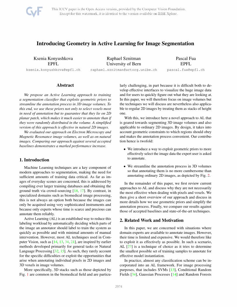
Figure 1. Interface of the FIJI Visualization API [25], which is
extensively used to interact with 3D image stacks. The user is
presented with three orthogonal planar slices of the stack. While
effective when working slice by slice, this is extremely cumbersome
for random access to voxels anywhere in the 3D stack, which is
what a naive AL implementation would require.
User User
inputinput
(a) (b)
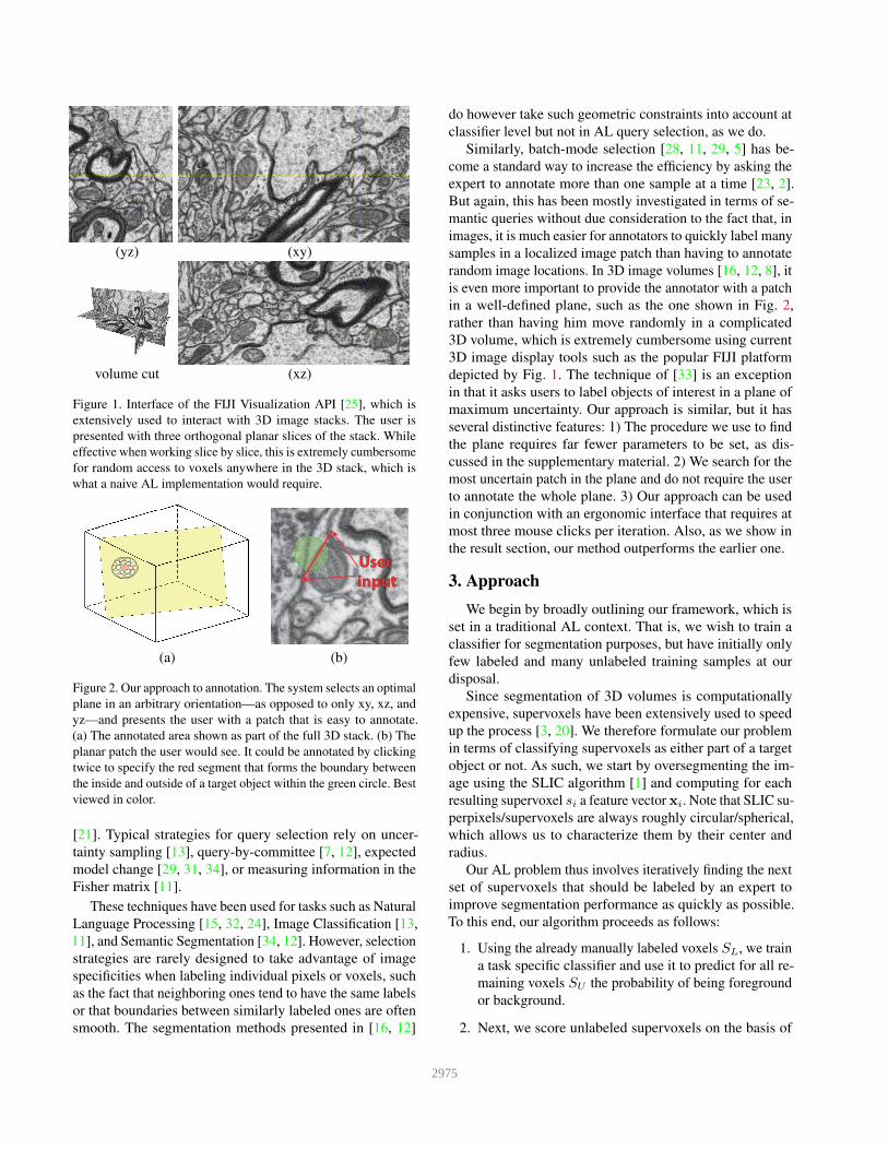
Figure 2. Our approach to annotation. The system selects an optimal
plane in an arbitrary orientation—as opposed to only xy, xz, and
yz—and presents the user with a patch that is easy to annotate.
(a) The annotated area shown as part of the full 3D stack. (b) The
planar patch the user would see. It could be annotated by clicking
twice to specify the red segment that forms the boundary between
the inside and outside of a target object within the green circle. Best
viewed in color.
[21]. Typical strategies for query selection rely on uncer-
tainty sampling [13], query-by-committee [7, 12], expected
model change [29, 31, 34], or measuring information in the
Fisher matrix [11].
These techniques have been used for tasks such as Natural
Language Processing [15, 32, 24], Image Classification [13,
11], and Semantic Segmentation [34, 12]. However, selection
strategies are rarely designed to take advantage of image
specificities when labeling individual pixels or voxels, such
as the fact that neighboring ones tend to have the same labels
or that boundaries between similarly labeled ones are often
smooth. The segmentation methods presented in [16, 12]
do however take such geometric constraints into account at
classifier level but not in AL query selection, as we do.
Similarly, batch-mode selection [28, 11, 29, 5] has be-
come a standard way to increase the efficiency by asking the
expert to annotate more than one sample at a time [23, 2].
But again, this has been mostly investigated in terms of se-
mantic queries without due consideration to the fact that, in
images, it is much easier for annotators to quickly label many
samples in a localized image patch than having to annotate
random image locations. In 3D image volumes [16, 12, 8], it
is even more important to provide the annotator with a patch
in a well-defined plane, such as the one shown in Fig. 2,
rather than having him move randomly in a complicated
3D volume, which is extremely cumbersome using current
3D image display tools such as the popular FIJI platform
depicted by Fig. 1. The technique of [33] is an exception
in that it asks users to label objects of interest in a plane of
maximum uncertainty. Our approach is similar, but it has
several distinctive features: 1) The procedure we use to find
the plane requires far fewer parameters to be set, as dis-
cussed in the supplementary material. 2) We search for the
most uncertain patch in the plane and do not require the user
to annotate the whole plane. 3) Our approach can be used
in conjunction with an ergonomic interface that requires at
most three mouse clicks per iteration. Also, as we show in
the result section, our method outperforms the earlier one.
3. Approach
We begin by broadly outlining our framework, which is
set in a traditional AL context. That is, we wish to train a
classifier for segmentation purposes, but have initially only
few labeled and many unlabeled training samples at our
disposal.
Since segmentation of 3D volumes is computationally
expensive, supervoxels have been extensively used to speed
up the process [3, 20]. We therefore formulate our problem
in terms of classifying supervoxels as either part of a target
object or not. As such, we start by oversegmenting the im-
age using the SLIC algorithm [1] and computing for each
resulting supervoxel si a feature vector xi. Note that SLIC su-
perpixels/supervoxels are always roughly circular/spherical,
which allows us to characterize them by their center and
radius.
Our AL problem thus involves iteratively finding the next
set of supervoxels that should be labeled by an expert to
improve segmentation performance as quickly as possible.
To this end, our algorithm proceeds as follows:
1. Using the already manually labeled voxels SL, we train
a task specific classifier and use it to predict for all re-
maining voxels SU the probability of being foreground
or background.
2. Next, we score unlabeled supervoxels on the basis of
2975
a novel uncertainty function that combines traditional
Feature Uncertainty with Geometric Uncertainty. Esti-
mating the former usually involves feeding the features
attributed to each supervoxel to the previously trained
classifier. To compute the latter, we look at the uncer-
tainty of the label that can be inferred based on a su-
pervoxel’s distance to its neighbors and their predicted
labels. By doing so, we effectively capture the con-
straints imposed by the local smoothness of the image
data.
3. We then automatically select the best plane through the
3D image volume in which to label additional samples,
as depicted in Fig. 2. The expert can then effortlessly
label the supervoxels from a circle in the selected plane
by defining a line separating target from non-target
regions. This removes the need to examine the relevant
image data from multiple perspectives, as depicted in
Fig. 1, and simplifies the labeling task.
The process is then repeated. In Sec. 4, we will discuss
the second step and in Sec. 5 the third. In Sec. 6, we will
demonstrate that this pipeline yields faster learning rates
than competing approaches.
4. Geometry-Based Active Learning
Most AL methods were developed for general tasks and
operate exclusively in feature space, thus ignoring the ge-
ometric properties of images and more specifically their
geometric consistency. To remedy this, we introduce the
concept of Geometric Uncertainty and then show how to
combine it with more traditional Feature Uncertainty.
Our basic insight is that supervoxels that are assigned a
label other than that of their neighbors ought to be consid-
ered more carefully than those that are assigned the same
labels. In other words, under the assumption that neighbors
more often than not have identical labels, the chance of the
assigment being wrong is higher. This is what we refer to as
Geometric Uncertainty and we now formalize it.
4.1. Feature Uncertainty
For each supervoxel si and each class y, let pθ(yi = y|xi)be the probability that its class yi is y, given the correspond-
ing feature vector xi. In this work, we will assume that this
probability can be computed by means of a classifier which
has been trained using parameters θ and we take y to be 1 if
the supervoxel belongs to the foreground and 0 otherwise 1.
In many AL algorithms, the uncertainty of this prediction is
taken to be the Shannon entropy
Hθi = −
∑
y∈{0,1}
pθ(yi = y|xi) log pθ(yi = y|xi). (1)
1Extensions to multiclass cases can be similarly derived.
pθ(yj1 = y)
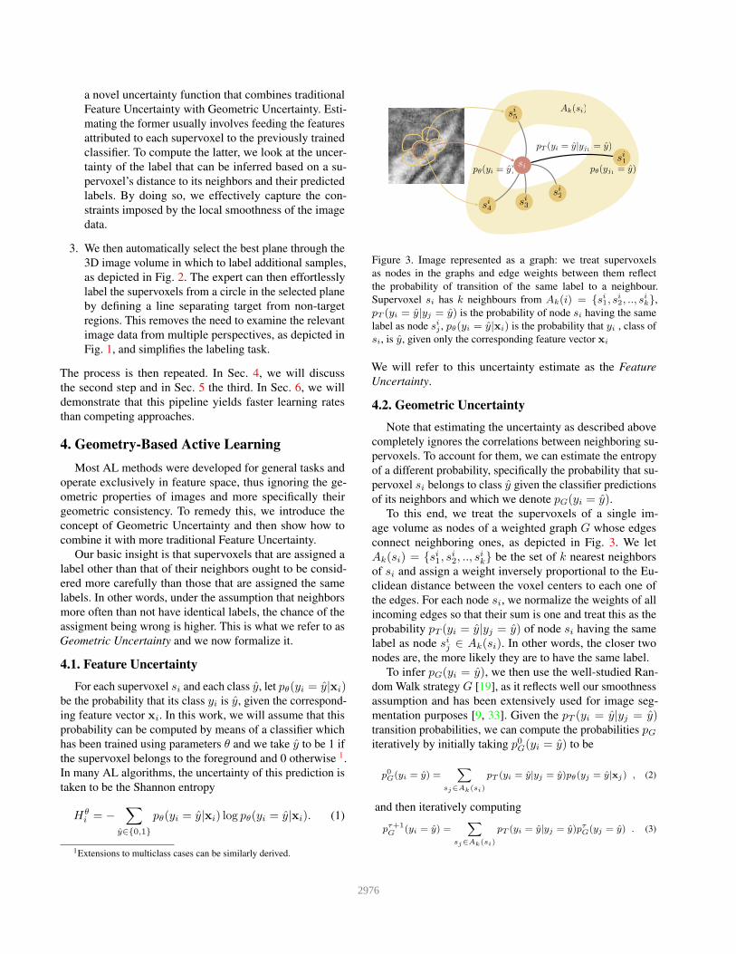
Figure 3. Image represented as a graph: we treat supervoxels
as nodes in the graphs and edge weights between them reflect
the probability of transition of the same label to a neighbour.
Supervoxel si has k neighbours from Ak(i) = {si1, si2, .., s
ik},
pT (yi = y|yj = y) is the probability of node si having the same
label as node sij , pθ(yi = y|xi) is the probability that yi , class of
si, is y, given only the corresponding feature vector xi
We will refer to this uncertainty estimate as the Feature
Uncertainty.
4.2. Geometric Uncertainty
Note that estimating the uncertainty as described above
completely ignores the correlations between neighboring su-
pervoxels. To account for them, we can estimate the entropy
of a different probability, specifically the probability that su-
pervoxel si belongs to class y given the classifier predictions
of its neighbors and which we denote pG(yi = y).To this end, we treat the supervoxels of a single im-
age volume as nodes of a weighted graph G whose edges
connect neighboring ones, as depicted in Fig. 3. We let
Ak(si) = {si1, si2, .., s
ik} be the set of k nearest neighbors
of si and assign a weight inversely proportional to the Eu-
clidean distance between the voxel centers to each one of
the edges. For each node si, we normalize the weights of all
incoming edges so that their sum is one and treat this as the
probability pT (yi = y|yj = y) of node si having the same
label as node sij ∈ Ak(si). In other words, the closer two
nodes are, the more likely they are to have the same label.
To infer pG(yi = y), we then use the well-studied Ran-
dom Walk strategy G [19], as it reflects well our smoothness
assumption and has been extensively used for image seg-
mentation purposes [9, 33]. Given the pT (yi = y|yj = y)transition probabilities, we can compute the probabilities pGiteratively by initially taking p0G(yi = y) to be
p0G(yi = y) =
∑
sj∈Ak(si)
pT (yi = y|yj = y)pθ(yj = y|xj) , (2)
and then iteratively computing
pτ+1G
(yi = y) =∑
sj∈Ak(si)
pT (yi = y|yj = y)pτG(yj = y) . (3)
2976
The procedure describes the propagation of labels to su-
pervoxels from its neighborhood. The number of iterations
τmax defines the radius of the neighborhood involved in the
computation of pG for si and encodes the smoothness priors.
Given these probabilities, we can now take the Geometric
Uncertainty to be
HGi = −
∑
y∈{0,1}
pG(yi = y) log pG(yi = y) , (4)
as we did in Sec. 4.1 to estimate the Feature Uncertainty.
4.3. Combining Feature and Geometric Entropy
As discussed above, from a trained classifier we can thus
estimate the Feature and Geometric Uncertainties. To use
them jointly, we should in theory estimate the joint proba-
bility distribution pθ,G(yi = y|xi) and the corresponding
joint entropy. As this is computationally intractable in our
model, we take advantage of the fact that the joint entropy
is upper bounded by the sum of individual entropies Hθ
and HG. Thus, for each supervoxel, we take the Combined
Uncertainty to be
Hθ,Gi = Hθ
i +HGi (5)
that is, the upper bound of the joint entropy.
In practice, using this measure means that supervoxels
that individually receive uncertain predictions and are in
areas of transition between foreground and background will
be considered first.
5. Batch-Mode Geometry Query Selection
The simplest way to exploit the Combined Uncertainty
introduced in Sec. 4.3 would be to pick the most uncer-
tain supervoxel, ask the expert to label it, retrain the clas-
sifier, and iterate. A more effective way however is to find
appropriately-sized batches of uncertain supervoxels and ask
the expert to label them all before retraining the classifier.
As discussed in Sec. 2, this is referred to as batch-mode
selection. A naive implementation of this would force the
user to randomly view and annotate supervoxels in the vol-
ume regardless of where they are, which would be extremely
cumbersome.
In this section, we therefore introduce an approach to
using the uncertainty measure to first select a planar patch
in 3D volumes and then to allow the user to quickly label
positives and negatives within it, a shown in Fig. 2.
Since we are working in 3D and there is no preferential
orientation in the data to work with, it makes sense to look
for spherical regions where the uncertainty is maximal. How-
ever, for practical reasons, we only want the annotator to
consider circular regions within planar patches such as the
one depicted in Fig. 2 and Fig. 4. These can be understood
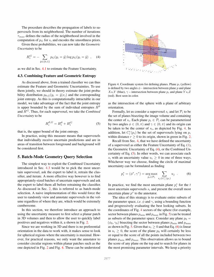
Figure 4. Coordinate system for defining planes. Plane pi (yellow)
is defined by two angles φ – intersection between plane p and plane
XsiY (blue), γ – intersection between plane pi and plane Y siZ
(red). Best seen in color.
as the intersection of the sphere with a plane of arbitrary
orientation.
Formally, let us consider a supervoxel si and let Pi to be
the set of planes bisecting the image volume and containing
the center of si. Each plane pi ∈ Pi can be parameterized
by two angles φ ∈ (0, π) and γ ∈ (0, π) and its origin can
be taken to be the center of si, as depicted by Fig. 4. In
addition, let Cri (pi) be the set of supervoxels lying on pi
within distance r ≥ 0 to its origin, shown in green in Fig. 2.
Recall from Sec. 4, that we have defined the uncertainty
of a supervoxel as either the Feature Uncertainty of Eq. (1),
the Geometric Uncertainty of Eq. (4), or the Combined Un-
certainty of Eq. (5). In other words, we can associate each
si with an uncertainty value ui ≥ 0 in one of three ways.
Whichever way we choose, finding the circle of maximal
uncertainty can be formulated as finding
p∗i = (φ∗, γ∗) = argmaxpi∈Pi
∑
sj∈Cri(pi)
uj . (6)
In practice, we find the most uncertain plane p∗i for the t
most uncertain supervoxels si and present the overall most
uncertain plane p∗ to the annotator.
The idea of this strategy is to evaluate entire subsets of
the parameter space, i.e. φ and γ, using a bounding function
and progressively evaluating the best looking subsets. In
the coordinates of Fig. 4 sectors of the sphere (for example,
sector between planes pmin and pmax in Fig. 5) can be treated
as subsets of the parameter space. Consider any plane p0 =(φ0, γ0) bisecting the sector between planes pmin and pmax
as shown in Fig. 5. Given that ui ≥ 0 and that Eq. (6) is linear
in ui ≥ 0, the score of the plane p0 will certainly be less
or equal to the score of all the points included between two
planes pmin and pmax. This observation allows us to bound
the score of any plane on the top and to search for planes in
the most promising parameter intervals. We keep a priority
2977

Figure 5. Bounding function and sector splitting procedure. The
score of the plane p0 is less or equal to the score of all the points
included between two planes pmin and pmax. Best seen in colour.
queue of sectors and at each step we divide the sector with
the highest uncertainty in two new sectors by a bisector plane
as in Fig. 5. The uncertainties of new sectors are computed
added to the priority queue. The optimal parameters are then
attained when the evaluated subset contain is a singleton.
Formal definitions and more details on the procedure are
given in the supplementary material.
By contrast to an exhaustive search that would be excru-
ciatingly slow, our current MATLAB implementation on the
10 images of resolution 176× 170× 220 of MRI dataset of
Sec. 6.3 takes 0.12s per plane selection at supervoxel. This
means that a C implementation would be real-time, which is
critical to such an interactive method to being accepted by
users.
Note that when the radius r = 0, this reduces to what
single-supervoxel labeling does. By contrast, for r > 0,
this allows annotation of many uncertain supervoxels with
a few mouse clicks, as will be discussed further in Sec. 6.
Although planar selection can be applied to any type of
uncertainty value, we believe that it is the most beneficial
when combined with Geometric Uncertainty as the latter
already takes into account the most uncertain regions instead
of isolated supervoxels.
6. Experiments
In this section, we evaluate our full approach both on two
different Electron Microscopy (EM) datasets and a Magnetic
Resonance Imaging (MRI) one. We then demonstrate that a
simplified version is effective for natural 2D Images.
6.1. Setup and Parameters
For all our experiments, we used Boosted Trees selected
by Gradient Boosting [30, 4] as our underlying classifier.
Given that during early AL iterations rounds, only limited
amounts of training data are available, we limit the depth
of our trees to 2 to avoid over-fitting. Following standard
practice, individual trees are optimized using 40% − 60%
of the available training data chosen at random and 10 to 40features are explored per split. We set the number k of near-
est neighbors of Section 4.2 to be the number of immediately
adjacent supervoxels on average, which is between 7 and 15
depending on the resolution of the image and size of super-
voxels. However, experiments showed that the algorithm is
not very sensitive to the choice of this parameter. We restrict
the size of each planar patch to be small enough to contain
typically not more than part of one object of interest. To this
end, the we take the radius r of Section 5 to be between
10 and 15, which yields patches such as those depicted by
Fig. 6.
Baselines. For each dataset, we compare our approach
against several baselines. The simplest is Random Sampling
(Rs), that is, randomly selecting samples to be labeled. It
serves to gauge the difficulty of the segmentation problem
and quantify the improvement brought by the more elaborate
strategies.
The next simplest, but widely accepted approach is to per-
form Uncertainty Sampling [5, 18] of supervoxel by using
the uncertainty measures of Section 4. Let HUi be the uncer-
tainty score we use in a specific experiment. The strategy
then is to select
s∗ = argmaxsi∈SU
(HUi ). (7)
We will refer to this as FUs when using the Feature Un-
certainty of Eq. 1 and as CUs when using the Combined
Uncertainty of Eq. 5. For the Random Walk, iterative pro-
cedure with τmax = 20 leads to high learning rates in our
applications. Finally, the most sophisticated approach is to
use Batch-Mode Geometry Query Selection, as described
in Sec. 5, in conjunction with either Feature Uncertainty or
Combined Uncertainty. We will refer to the two resulting
strategies as pFUs and pCUs, respectively. Both plane se-
lection strategies are using t = 5 best supervoxels in the
optimization. Further increase of this value didn’t demon-
strate significant growth of the learning rate.
Fig. 2, 6 jointly depict what a potential user would see for
pFUs and pCUs given a small enough patch radius. Given a
well designed interface, it will typically require to click only
once or twice to provide the required feedback (see Fig. 6). In
our performance evaluation, we will therefore estimate that
each intervention of the user for pFUs and pCUs requires
two clicks whereas for Rs, FUs, and CUs it requires only
one. So, for the method comparison we measure annotation
effort as 1 for Rs, FUs, and CUs and as 2 for pFUs and
pCUs.
Note that pFUs is similar in spirit to the approach of [33]
and can therefore be taken as a good indicator of how this
other method would perform on our data. However, un-
like [33], we do not require user to label the whole plane and
keep our suggested interface for a fairer comparison.
2978

Figure 7. Estimate mean and standard deviation for classifier scores
of positive class datapoints (red) – µ+ and σ+ and negative class
datapoints (blue) – µ−, σ−, and fit 2 Gaussian distributions. Given
their pdf estimate optimal Bayesian error with threshold h∗.
Adpative Thresholding. Recall from Section 4.1 that for
all the approaches discussed here, the probability of a su-
pervoxel being foreground is computed as pθ(yi = 1|xi) =(1+ exp−2·(F−h))−1, where F is the output of the classifier
and h is the threshold [10]. Usually, the threshold is cho-
sen by cross-validation but this strategy may be misleading
or not even possible for AL. We therefore assume that the
scores of training samples in each class are Gaussian dis-
tributed with unknown parameters µ and σ. We then find
an optimal threshold h∗ by fitting Gaussian distributions to
the scores of positive and negative classes and choosing the
value that yields the smallest Bayesian error, as depicted by
Fig. 7. We refer to this approach as Adaptive Thresholding
and we use it for all our experiments.
Experimental Protocol. In all cases, we start with 5 pos-
itive and 5 negative labeled supervoxels and perform AL
iterations until we receive 100 inputs from the user. Each
method starts with the same random subset of samples and
each experiment is repeated N = 40 times. We will therefore
plot not only accuracy results but also indicate the variance
of these results.
Fully annotated volumes of ground truth are available for
us and we use them to simulate the expert’s intervention in
our experiments. We detail the specific features we used for
EM, MRI, and natural images below.
6.2. Results on EM data
Here, we work with two 3D Electron Microscopy stacks
of rat neural tissue, one from the striatum and the other
from the hippocampus. One stack of size 318× 711× 422(165×1024×653 for hippocampus) is used for training and
another stack of size 318× 711× 450 (165× 1024× 883)
is used to evaluate the performance. Their resolution is 5nm
in all three spatial orientations. The slices of Fig. 1 as well
as patches in the upper row in Fig. 6 come from the striatum
and hippocampus volume is shown in Fig. 9 with its patches
shown in the lower row of Fig. 6.
The task is to segment mitochondria, which are the intra-
cellular structures that supply the cell with its energy and are
of great interest to neuroscientists. It is extremely laborious
to annotate sufficient amounts of training data for learning
segmentation algorithms to work satisfactorily. Furthermore,
different brain areas have different characteristics, which
means that the task must be repeated often. The features
we feed our Boosted Trees rely on local texture and shape
information using ray descriptors and intensity histograms
as in [20].
Dataset FUs CUs pFUs pCUs
Hippocampus 0.1172 0.1009 0.0848 0.0698
Striatum 0.1326 0.1053 0.1133 0.0904
MRI 0.0758 0.0642 0.0767 0.0545
Natural 0.1448 0.1389 0.1494 0.1240
Table 1. Variability of results by different AL strategies. 80% of the
scores are lying within the indicated interval. Feature Uncertainty
is always more variable that Combined Uncertainty, batch selection
is always less variable that single-instance selection. The best result
is highlighted in bold.
In Fig. 8, we plot the performance of all the approaches
we consider in terms of the VOC [6] score, a commonly used
measure for this kind of application, as a function of the
annotation effort. The horizontal line at the top depicts the
VOC scores obtained by using the whole training set, which
comprises 276130 and 325880 supervoxels, for the striatum
and the hippocampus respectively. FUs provides a boost
over Rs, and CUs yields a larger one. In both cases, a further
improvement is obtained by introducing the batch-mode
geometry query selection of pFUs and pCUs, with the latter
coming on top. Recall that these numbers are averages over
many runs. In Table 1, we give the corresponding variances.
Note that both using the Geometric Uncertainty and the
batch-mode tend to reduce them, thus making the process
more predictable. Note also the 100 number we use very
much smaller than the total number of available samples.
Somewhat surprisingly, in the hippocampus case, the clas-
sifier performance given only 100 training data points is
higher that the one obtained by using all the training data.
In fact, this phenomenon has been reported in the AL litera-
ture [26] and suggests that a well chosen subset of datapoints
can produce better generalisation performance than the com-
plete set.
6.3. Results on MRI data
Here we consider multimodal brain tumor segmentation
in MRI brain scans. Segmentation quality depends critically
on the amount of training data and only highly-trained ex-
perts can provide it. T1, T2, FLAIR, and post-Gadolinium T1
MR images are available in the BRATS dataset for each one
2979
(a)
(b)
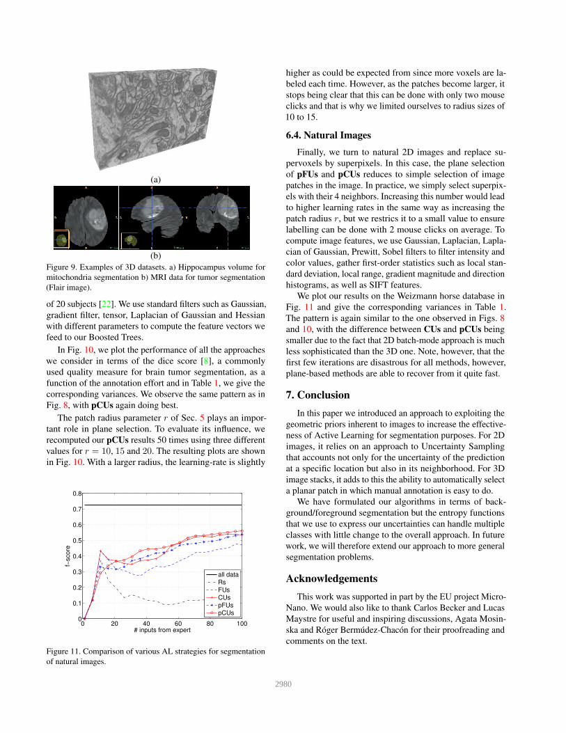
Figure 9. Examples of 3D datasets. a) Hippocampus volume for
mitochondria segmentation b) MRI data for tumor segmentation
(Flair image).
of 20 subjects [22]. We use standard filters such as Gaussian,
gradient filter, tensor, Laplacian of Gaussian and Hessian
with different parameters to compute the feature vectors we
feed to our Boosted Trees.
In Fig. 10, we plot the performance of all the approaches
we consider in terms of the dice score [8], a commonly
used quality measure for brain tumor segmentation, as a
function of the annotation effort and in Table 1, we give the
corresponding variances. We observe the same pattern as in
Fig. 8, with pCUs again doing best.
The patch radius parameter r of Sec. 5 plays an impor-
tant role in plane selection. To evaluate its influence, we
recomputed our pCUs results 50 times using three different
values for r = 10, 15 and 20. The resulting plots are shown
in Fig. 10. With a larger radius, the learning-rate is slightly
0 20 40 60 80 1000
0.1
0.2
0.3
0.4
0.5
0.6
0.7
0.8
# inputs from expert
f−score
all dataRsFUs
CUspFUspCUs
Figure 11. Comparison of various AL strategies for segmentation
of natural images.
higher as could be expected from since more voxels are la-
beled each time. However, as the patches become larger, it
stops being clear that this can be done with only two mouse
clicks and that is why we limited ourselves to radius sizes of
10 to 15.
6.4. Natural Images
Finally, we turn to natural 2D images and replace su-
pervoxels by superpixels. In this case, the plane selection
of pFUs and pCUs reduces to simple selection of image
patches in the image. In practice, we simply select superpix-
els with their 4 neighbors. Increasing this number would lead
to higher learning rates in the same way as increasing the
patch radius r, but we restrics it to a small value to ensure
labelling can be done with 2 mouse clicks on average. To
compute image features, we use Gaussian, Laplacian, Lapla-
cian of Gaussian, Prewitt, Sobel filters to filter intensity and
color values, gather first-order statistics such as local stan-
dard deviation, local range, gradient magnitude and direction
histograms, as well as SIFT features.
We plot our results on the Weizmann horse database in
Fig. 11 and give the corresponding variances in Table 1.
The pattern is again similar to the one observed in Figs. 8
and 10, with the difference between CUs and pCUs being
smaller due to the fact that 2D batch-mode approach is much
less sophisticated than the 3D one. Note, however, that the
first few iterations are disastrous for all methods, however,
plane-based methods are able to recover from it quite fast.
7. Conclusion
In this paper we introduced an approach to exploiting the
geometric priors inherent to images to increase the effective-
ness of Active Learning for segmentation purposes. For 2D
images, it relies on an approach to Uncertainty Sampling
that accounts not only for the uncertainty of the prediction
at a specific location but also in its neighborhood. For 3D
image stacks, it adds to this the ability to automatically select
a planar patch in which manual annotation is easy to do.
We have formulated our algorithms in terms of back-
ground/foreground segmentation but the entropy functions
that we use to express our uncertainties can handle multiple
classes with little change to the overall approach. In future
work, we will therefore extend our approach to more general
segmentation problems.
Acknowledgements
This work was supported in part by the EU project Micro-
Nano. We would also like to thank Carlos Becker and Lucas
Maystre for useful and inspiring discussions, Agata Mosin-
ska and Róger Bermúdez-Chacón for their proofreading and
comments on the text.
2980

(a) (b) (c)
Figure 6. Circular patches to be annotated by the expert highlighted by the yellow circle in (a) Electron Microscopy data, (b) MRI data,
and (c) natural images. The patches can be entirely foreground, entirely background. Alternatively, the boundary between foreground an
background within the patch can be indicated by tracing a red line segment. In all cases, that would require at most two mouse clicks.
0 20 40 60 80 1000
0.1
0.2
0.3
0.4
0.5
0.6
0.7
0.8
# inputs from expert
VO
C s
co
re
all dataRsFUs
CUspFUspCUs
0 20 40 60 80 1000
0.1
0.2
0.3
0.4
0.5
0.6
0.7
0.8
# inputs from expert
VO
C s
co
re
all dataRsFUs
CUspFUspCUs
(a) (b)
Figure 8. Comparison of various AL strategies for mitochondria segmentation. Left: striatum dataset, right: hippocampus dataset.
0 20 40 60 80 1000
0.1
0.2
0.3
0.4
0.5
0.6
0.7
0.8
0.9
# inputs from expert
dic
e s
co
re
all dataRsFUs
CUspFUspCUs
0 20 40 60 80 1000
0.1
0.2
0.3
0.4
0.5
0.6
0.7
0.8
0.9
# inputs from expert
dic
e s
co
re
radius 10
radius 15
radius 20
(a) (b)Figure 10. Comparison of various AL strategies for MRI data for tumor segmentation. Left: dice score for BRATS2012 dataset, right: pCUs
strategy with patches of different radius.
2981
References
[1] R. Achanta, A. Shaji, K. Smith, A. Lucchi, P. Fua, and
S. Suesstrunk. SLIC Superpixels Compared to State-Of-The-
Art Superpixel Methods. IEEE Transactions on Pattern Anal-
ysis and Machine Intelligence, 34(11):2274–2282, November
2012.
[2] A. Al-Taie, H. H. K., and L. Linsen. Uncertainty Estimation
and Visualization in Probabilistic Segmentation. 2014.
[3] B. Andres, U. Koethe, M. Helmstaedter, W. Denk, and F. Ham-
precht. Segmentation of SBFSEM Volume Data of Neural
Tissue by Hierarchical Classification. In DAGM Symposium
on Pattern Recognition, pages 142–152, 2008.
[4] C. Becker, R. Rigamonti, V. Lepetit, and P. Fua. Supervised
Feature Learning for Curvilinear Structure Segmentation. In
Conference on Medical Image Computing and Computer As-
sisted Intervention, September 2013.
[5] E. Elhamifar, G. Sapiro, A. Yang, and S. S. Sasrty. A Convex
Optimization Framework for Active Learning. In Interna-
tional Conference on Computer Vision, 2013.
[6] M. Everingham, C. W. L. Van Gool and, J. Winn, and
A. Zisserman. The Pascal Visual Object Classes Chal-
lenge (VOC2010) Results, 2010.
[7] R. Gilad-Bachrach, A. Navot, and N. Tishby. Query By
Committee Made Real. In Advances in Neural Information
Processing Systems, 2005.
[8] N. Gordillo, E. Montseny, and P. Sobrevilla. State of the
Art Survey on MRI Brain Tumor Segmentation. Magnetic
Resonance in Medicine, 2013.
[9] L. Grady. Random Walks for Image Segmentation. IEEE
Transactions on Pattern Analysis and Machine Intelligence,
28(11):1768–1783, 2006.
[10] T. Hastie, R. Tibshirani, and J. Friedman. The Elements of
Statistical Learning. Springer, 2001.
[11] S. C. H. Hoi, R. Jin, J. Zhu, and M. R. Lyu. Batch Mode
Active Learning and its Application to Medical Image Classi-
fication. In International Conference on Machine Learning,
2006.
[12] J. Iglesias, E. Konukoglu, A. Montillo, Z. Tu, and A. Cri-
minisi. Combining Generative and Discriminative Models
for Semantic Segmentation. In Information Processing in
Medical Imaging, 2011.
[13] A. Joshi, F. Porikli, and N. Papanikolopoulos. Multi-Class
Active Learning for Image Classification. In Conference on
Computer Vision and Pattern Recognition, 2009.
[14] A. Kapoor, K. Grauman, R. Urtasun, and T. Darrell. Active
Learning with Gaussian Processes for Object Categorization.
In International Conference on Computer Vision, 2007.
[15] D. Lewis and W. Gale. A Sequential Algorithm for Training
Text Classifiers. 1994.
[16] Q. Li, Z. Deng, Y. Zhang, X. Zhou, U. V. Nagerl, and S. T. C.
Wong. A Global Spatial Similarity Optimization Scheme to
Track Large Numbers of Dendritic Spines in Time-Lapse Con-
focal Microscopy. IEEE Transactions on Medical Imaging,
30(3):632–641, 2011.
[17] T.-Y. Lin, M. Maire, S. Belongie, J. Hays, P. Perona, D. Ra-
manan, P. Dollár, and C. Zitnick. Microsoft COCO: Common
objects in context. In European Conference on Computer
Vision, pages 740–755, 2014.
[18] C. Long, G. Hua, and A. Kapoor. Active Visual Recognition
with Expertise Estimation in Crowdsourcing. In International
Conference on Computer Vision, 2013.
[19] L. Lovász. Random Walks on Graphs: A Survey. Combina-
torics, Paul Erdos is Eighty, 1993.
[20] A. Lucchi, K. Smith, R. Achanta, G. Knott, and P. Fua.
Supervoxel-Based Segmentation of Mitochondria in EM Im-
age Stacks with Learned Shape Features. IEEE Transactions
on Medical Imaging, 31(2):474–486, February 2012.
[21] J. Maiora and M. G. na. Abdominal CTA Image Analysis
through Active Learning and Decision Random Forests: Apli-
cation to AAA Segmentation. In IJCNN, 2012.
[22] B. Menza, A. Jacas, et al. The Multimodal Brain Tumor Image
Segmentation Benchmark (BRATS). IEEE Transactions on
Medical Imaging, 2014.
[23] S. D. Olabarriaga and A. W. M. Smeulders. Interaction in the
Segmentation of Medical Images : A Survey. Medical Image
Analysis, 2001.
[24] F. Olsson. A Literature Survey of Active Machine Learning
in the Context of Natural Language Processing. Swedish
Institute of Computer Science, 2009.
[25] B. Schmid, J. Schindelin, A. Cardona, M. Longair, and
M. Heisenberg. A High-Level 3D Visualization API for Java
and ImageJ. BMC Bioinformatics, 11:274, 2010.
[26] G. Schohn and D. Cohn. Less is more: Active learning with
support vector machines. In ICML, 2000.
[27] B. Settles. Active Learning Literature Survey. Computer
Sciences Technical Report 1648, University of Wisconsin–
Madison, 2010.
[28] B. Settles. From Theories to Queries : Active Learning in
Practice. Active Learning and Experimental Design, 2011.
[29] B. Settles, M. Craven, and S. Ray. Multiple-Instance Active
Learning. In Advances in Neural Information Processing
Systems, 2008.
[30] R. Sznitman, C. Becker, F. Fleuret, and P. Fua. Fast Object
Detection with Entropy-Driven Evaluation. In Conference on
Computer Vision and Pattern Recognition, pages 3270–3277,
2013.
[31] R. Sznitman and B. Jedynak. Active Testing for Face Detec-
tion and Localization. IEEE Transactions on Pattern Analysis
and Machine Intelligence, 32(10):1914–1920, June 2010.
[32] S. Tong and D. Koller. Support Vector Machine Active Learn-
ing with Applications to Text Classification. Machine Learn-
ing, 2002.
[33] A. Top, G. Hamarneh, and R. Abugharbieh. Active learning
for interactive 3D image segmentation. Conference on Med-
ical Image Computing and Computer Assisted Intervention,
2011.
[34] A. Vezhnevets, J. Buhmann, and V. Ferrari. Active Learning
for Semantic Segmentation with Expected Change. In Con-
ference on Computer Vision and Pattern Recognition, 2012.
2982